/^

RADC-TR-76-189 Final Technical Report June 1976

O

TURBULENCE CHARACTERIZATION AND CONTROL

Avco Everett Research Laboratory, Inc.

Sponsored By Defense Advanced Research Projects Agency

ARPA Order No. 2646

Approved for public release; distribution unlimited.

The views and conclusions contained in this document are those of the authors aud should not be interpreted as necessarily representing the official policies, either expressed or Implied, of the Defense Advanced Research Projects Agency or the U. S. Government.

ROME AIR DEVELOPMENT CENTER AIR FORCE SYSTEMS COMMAND

GRIFFISS AIR FORCE BASE. NEW YORK 13441 ßr

D D C ,r7^r3nn nr?

1976

This report has been reviewed by the RADC Information Office (01) and is «leasable to the National Technical Information Service ^NTIS). At NTIS it will be releasable to the general public, including foreign nations,

This report has been reviewed and approved for publication.

APPROVED:

DONALD W. HANSON Project Engineer

KA*^

Do not return this copy. Retain or destroy.

MISSION of

Rome Air Development Center

FADC is the principal AFSC organization charged with planning and executing the USAF exploratory and advanced development programs for information sciences, intelli- gence, command, control and communications te^°l0*J' products and services oriented to the needs of the USAF. Primary RADC mission areas are communications, electro- magnetic guidance and control, surveillance of ground and aerospace objects, intelligence data collection and handling, information system technology, and electronic reliability, maintainability and f^^bUm. M* has mission responsibility as assigned by *FSC tor ae

monstration and acquisition of ^^V^^o^nd * systems in the intelligence, capping, charting, command, 9 control and communications areas. ^b

^2\ ^6-l916

TURBULENCE CHARACTERIZATION AND CONTROL

M. G. Miller p. L. Zleske G. Dryden

Contractor: Avco Everett Research Laboratory. Inc.

Contract Number: F30602-75-C-0012 Effective Date of Contract: 1 August 1974 Contract Expiration Date: 15 October 1975

Program Code Number: 5E20 Period of work covered: Feb 75 - Or.t 75

Principal Investigator: Phone:

Dr. Merlin G. Miller 617 389-300 Ext. 528

Project Engineer; Donald W. Hanson

Phone: 315 330--3145

Approved for public release; distribution unlimited.

This research was supported by the Defense Advanced Research Projects Agency of the Department of Defense and was monitored by Donald W. Hanson (OCSE),

Griffiss AFB NY 13441.

UNCLASSIFIED SECURITY Ci.ASSIFir^TION OF THIS "»OE <**»" Data Enured)

T/fi REPORT DOCUMENTATION PAGE NUWDER 2. GOVT ACCESSION NO

RADC4TR-76-189 | 4. TITLE (and Subtitle)

TURBULENCE CHARACTERIZATION AND CONTROL, •3r .• JS

79]

READ INSTRUCTIONS BEFORE COMPLETING FORM

3. RECIPIENT'S CATALOG NUMBER

v^W

I* MTG./Miller ' P. L. Zieske G./Dryden ,.,..■

X. ■T'ERrÖRMING'oRGANIZATION NAME AND ADDRESS

Avco Everett Research Laboratory, Inc. 2385 Revere Beach Parkway Evetett MA 02149

(/,

s, 'TYFVOF, REPORT »,P&J«|0,8»COVERED

Final /ecünlcal Rep«ct , i 1 Feb>5 - 15 Oct 75„ /

6. PERFORMING ORG. fiZ^OW^-HXSÜ

N/A B. CONTRACT OR GRANT NUMBERftJ

L Tj F3O6Ö2-75-C-O012,

•t,"ra:^gr:^MÜÜ^1i><'if<?M;ENT.'pRbjECT, T AREA A WORK UNIT NUMBERS

11. CONTROLLING OFFICE NAME AND ADDRESS Defense Advanced Research Projects Agency 1400 Wilson Blvd Arlington VA 22209

m T4. MONITORING AGENCY NAME » ADORESSf" dllfant from Controlllnt Olllca)

Rome Air Development Center (OCSE) Griffiss AFB NY 13441

12. REPQ.BT DATS

Jun**i(976 -mi»^»v>v | ——■

13. NUMBER OF PAGEV / /T/

15. SECURITY CLASS, fo/ (h/» report^ / ;—

UNCLASSIFIED 15a DECLASSIFICATION/OOWNGRADING N/ASCHEDULE

16. DISTRIBUTION STATEMENT (ol Ihit Report)

Approved for public release; distribution unlimited.

17. DISTRIB

Same

UTION STATEMENT (ol th, ab.tract entar.d In Block 20. II dlll.ranl Irom R.port)

18. SUPPLEMENTARY NOTES

RADC Project Engineer: Donald W. Hanson (OCSE)

4 id ABSTRACT This repoi

19 KEY WORDS rCondnue on rev.r.e ,ldo II n,c*,.ary and Idontlly by block number)

1. Atmospheric Optics 2. Turbulence 3. Seeing

^o^rc^;—mit^'^llt^e't^ the Äcterization of the turbulent environment at the ARPA Maui Observation Station. Three areas are discussed. ^1 firstdeals wxch the deployment of various instrumental systems to be used in the experimental program. These include micrometeorologlcal ^nsors a computer data processing system, and Acoustic Sounder, the NO^A Bt« Sensor and the Hughes Seeing Monitor which are all presently oper^tir. il.^.

Initial operations with the Seeing Monitor were carried out to August 1975 ': ^1 QQ fORM ^^J ED|T|0N OF 1 NOV 65 IS OBSOLETE UNCLASSIFIED

SECURITY CLASSIFICATION OF THIS PAGE (Whan Data Entered)

o'/f 'i^0

/*•

UNCLASSIFIED- SECURITY CLASSIFICATION OF THIS PAGEfWh.n P.I. Enl„.d)

I- .f ^OBO teats, we concluded that this device Is performing In

experiments.

of firstl and second order statistical properties down to the basic one

millisecond resolution time of device.

UNCLASSIFIED

SECUHI TY CLASSIFICATION OF THIS PAGEfWh.n Da(. ErK.r.d;

PREFACE

This report is submitted in compliance with the requirements of Contract #F30602-75-C-0012 and covers work carried out during the period I FebrStry 1975 to 15 October 1975. Previous work under *is contract is reported in RADC-TR-7C - 185 (July 1975).

We would like to thank the AMOS staff for assistance during the hard-

Refearch Laboratories, the Rome Air Development Center and the Hughes Research Laboratories.

-5/6-

TABLE OF CONTENTS

Section

1. 0

2.0

3. 0

4.0

Preface

INTRODUCTION

1.1 Background and Objectives

1.2 Program Status

EXPERIMENTAL INSTRUMENTATION

2. 1 Real-Time Data Processing System

2. 2 Routine Meteorological Sensors

2. 3 Microthermal Sensors

2.4 Seeing Monitor

2. 5 Small Aperture Photometer

2. 6 Acoustic Sounder

2.7 Star Sensor

INITIAL SEEING MONITOR TESTS

3. 1 Functional Tests

3. 2 Data Receiver

3. 3 Magnetic Tape Recording

3.4 Field-of-View

3. 5 Focus Test

3. 6 Image Rotation

3. 7 Analog Seeing Outputs

3. 8 Noise Characteristics

3. 9 Atmospheric Data

3. lOConclusion

SEEING MONITOR DATA REDUCTION SOFTWARE

References

Page

5

11

11

12

13

13

15

17

20

24

24

27

35

35

36

36

36

36

39

39

42

42

45

49

61

-7/8-

LIST OF ILLUSTRATIONS

Figure

2-7

Page

2-1 AMOS Site Locations of Atmospheric Instrumentation 14

2-2 Partial View of Atmospherics Data Recording Center Showing PDP-8/I Computer, A/D Converter and Sensor Patch Panel

16

2-3 North Meteorological Tower l8

2-4 Fat Wire Microthermal Probe, Partially Disassembled to 19 Show Integral Electronics

2-5 ASP/SM Combination Shown Mounted on the Side Blanchard 21 of the 48-inch, b=37 Telescope

2-6 Seeing Monitor Control Console Outputs on Front Panel 22 Provide Serial Digital Words for Seeing Angle and Wander Data

B=29 Photometer Console 25

2-8 External View of Acoustic Sounder Transducer Dish and 26 Anechoic Cuff

2-9 Internal View ox Acoustic Transducer, Dish and Anechoic Cuff

2-10 Acoustic Sounder Control Console

2-11 Celestron-14 Telescope with Star Sensor Electro-Optics Package Attached

2-12 NOVA 2/10 Computer, High Speed Paper Tape Pleader, 32 A/D Converter and Teletype used to Generate C^ Profile Data from Star Sensor Output in Realtime

28

29

30

38

40

3-1 Seeing Monitor: Field-of-View 3'

3-2 Seeing Monitor: Focus Test

3-3 Seeing Monitor: Seeing Angle Analog Output

3-4 Seeing Monitor: Analog Output Calibration 41

-9-

Figure PaSe

3-5 Seeing Monitor: Magnitude Sequence 43

3-6 Seeing Monitor: Data Summary 44

3-7 Seeing Monitor: Zenith Angle Dependence 46

4-la Flow Chart of Seeing Monitor Data Reduction Program 52

4-lb Flow Chart of Seeing Monitor Data Reduction Program 53

4-lc Flow Chart of Seeing Monitor Data Reduction Program 54

4-ld Flow Chart of Seeing Monitor Data Reduction Program 55

4-le Flow Chart of Seeing Monitor Data Reduction Program 56

4-2 Sample Plot of Seeing Monitor Simulated Data 57

4-3 Display of One Second Averages of Raw Simulated Seeing 58 Monitor Data with Error Bars

4-4 Sample Plot of Histogram of Simulated Seeing Monitor 59 Data

•10-

1. 0 INTRODUCTION

1.1 BACKGROUND AND OBJECTIVES

A major influencr on the operation of large optical systems arises from random phase and amplitude perturbations introduced into a propa- gating optical field by atmospheric turbulence. The origin of these effects are local small scale, temperature fluctuations which, in turn, produce variations in the index of refraction. These random perturbations in the received field are very significant in imaging systems because they limit resolution to the order of one or more arc seconds. A variety of tech- niques(1)-(6) have been proposed and in some cases implemented which minimize these effects to some degree. Experimental data is desirable for the evaluation, design and implementation of these systems.

In order to satisfy this data requirement, a set of atmospheric tur- bulence characterization experiments have been developed and are being implemented. Included are a variety of instrumentation which measure properties of the turbulent environment and its effects on optical Propagation. The site of these measurements is the ARPA Maui Optical Station (AMOS) atop Haleakala on the Island of Maui, Hawaii. The experimental objectives are to establish a data base on the long and short term statistics of atmos- pheric seeing conditions and provide input to the design of the Compensated Imaging Field System.

This program. Turbulence Characterization and Control, involves a number of specific tasks which fall into the following three general categories;

• Installation and checkout of experimental systems

• Data collection, reduction and interpretation

• Investigation of local turbulence created by the observatory and its operations.

During the first six months of this contract (1 August 1974 - 31 Jan- uary 1975), most effort was confined to the third area. In particular, the original site survey data was examined, an optical angle-of-arnval experi- ment was developed and implemented and a survey of turbulence control practices was carried out. The results of these studies are given in other reports. (12M13)

During the last half of this contract, effort was concentrated in the first two areas and is reported here. The status of the program as of the end of the contractual period is given below. Section 2. 0 details the instru- mental systems as they are presently deployed at AMOS. The result of the

-11-

initial tests with the Seeing Monitor are given in Section 3. 0. Software development for the deta^ed processing of the Seeing Monitor digital seeing angle outputs is given in the final section.

1. 2 PROGRAM STATUS

As of the date of this report, the status of the experimental systems are as follows:

• Microthermal and meteorological instrumentation have been installed on two towers exterior to the observatory.

• The PDP-8 data processing system for use specifically with the micromet system is operational.

• The NOAA Star Sensor has been installed in the AMOS Teal Amber dome and is operational.

• The Acoustic Sounder has been installed.

• The Seeing Monitor has been acceptance tested and is operational

• The Real-Time Atmospheric Measurement System has not yet been delivered.

Other accomplishments include:

• An initial period of operations with the Seeing Monitor

• Software development for the detailed processing of Seeing Monitor data.

In addition to the above, a detailed experimental plan for a first extensive period of data collection using all available instrumentation was developed. Several special experiments are also to be included in this series. The experimental period is scheduled for late fall, 1975 and will be reported on in the next technical report.

• 12-

2. 0 EXPERIMENTAL INSTRUMENTATION

In 1975 plans were formulated to install extensive instrumentation capable of characterizing atmospheric turbulence at the AMOS lite. A variety of instrumentation was selected to provide characterization data from ground level to the top of the atmosphere with as few gaps as possbile. In addition, because many of the sensors were to be prototypes, it was desired to have redundancy in the measurements to obtain an estimate of internal self-consistency.

Six separate instrument systems were installed at the Observatory starting mid-summer 1975. These were:

1) Routine meteorological sensors consisting of two (one north and one south of the East Dome) wind speed and wind direction instruments, one ambient temperature and one dew point sensor ;north only) mounted on towers,

2) Micrometeorological sensors consisting of six microthermal probes mounted as triads atop both towers.

3) The Seeing Monitor, a spinning reticle photometer, located on the side Blanchard of the 48-inch, b = 37 telescope.

4) A Small Aperture Photometer located on the 48-inch, b = 29 telescope.

5) The Acoustic Sounder, an echosonde device located approximately 50 m west of the Observatory.

6) The Star Sensor, a Cn2 profile device mounted on its own 3b cm

(14-inch) Schmidt-Cassegrain telescope.

Figure 2-1 shows the location of these sensors on the AMOS site. In addition to the above, a real-time data processing system utilizing a PDP-8/I Computer has been incorporated into the complete data collection system.

2. 1 REAL-TIME DATA PROCESSING SYSTEM

Because of the great quantity of data that these sensors can produce, it was desirable to automatically preprocess and reduce as much of the raw data as possible in real-time. To accomplish this, a computer with an analog-to-digital converter was made the real-time focal point of the Routine and Micrometeorological sensor systems. Seeing Monitor and Small Aperture Photometer data outputs can also be processed by this

-13-

Fig. 2-1 AMOS Site Locations of Atmospheric Instrumentation, A) Acoustic Sounder antenna; B) GLOS apparatus; C) West Dome, housing 48-inch, b=37 and b=29 tele- scopes; D) 16-foot dome housing Celestron-14 tele- scope and star sensor; E) North meteorological tower; F) South meteorological tower.

14-

system. The computer is a Digital Equipment Corporation PDP-8/I with 4K of rore. The machine has a 12-bit word (11 bits plus sign) and has a minimum cycle time of 800 ns. The basic input/output peripheral is a type 33 ASR teletype. Program material may be keyed in or read in from the paper tape reader. Sensor data input to the computer is through an analog-to-digital converter DEC model AD01-AN. The system has a multiplexer switch presently configured for 16 channes each with a bi- polar resolution of 10 bits (plus sign bit) or 1 part in 1024. Channel selection is program-selectable by a five-bit code. The converter is also equipped with a'sample and hold amplifier that produces a 100 ns conversion aperture. System accuracy is 0. 125% of full scale input. Throughput rate is 34 kHz (29 us) The converter has 4 programmable gain settings, 0 to + 1 25 + 2 5 + 5 and + 10 V full scale. These gain settings are program- lelectabfe withl two-bit code. Input impedance is 1000 -^hms in parallel with 20 pF, cross-channel attenuation is 78 db. The AD01-AN is capable of operating in two modes, interrupting or non-interrupting as selected by the program. Figure 2-2 shows the basic PDP-8/1 mainframe, analog-to-digital converter and teletype.

The PDP-8/1 computer system is operated with a maching language program that calculates means, variances and covariances for each of the input channels. Twelve channels are utilized by the Meteorological outputs fo? real-time data acquisition and processing. The additional four channels can be used for other sensors. The program allows each channel to be sampled "n" times (program selectable) and after "n" samples have been accumulated for all channels, the means and variances for each channel are computed as well as the covariances between channels. These final data are then printed out on the teletype in matrix form at 100 characters per minute.

2. 2 ROUTINE METEOROLOGICAL SENSORS

The meteorological sensors are located on two extendable towers (maximum height 18. 3 m) located north and south of the East Dome see Figure 2-1. Wind speed and wind direction sensors are mounted on both towers at the 17.4 m level. The instruments are Meteorology Research, inc. , Model 1074-2 combined cup and vane units. The wind speed sensor has a starting threshold of 0. 34 m/s, a response distance °f *J ^ m 63% recovery), a flow coefficient of 2.41 m/rev and an accuracy of + 0. 11 m/s. Upper wind speed limit is 55 m/s. The sensor uses a chopper wheel to produce a pulse train approximately 4 V peak-to-peak varying in ^quency From 0 to 2500 Hz; impedance is less than 10 K ohms. The signal is cabled to a transmuter which conditions the signal by means of a tachometer cir- cuit to produce an analog DC voltage ranging from 0 to + 5 V from an im- pedance of less than 1 K ohms. These signals are then cabled from the towers to the input side of the PDP-8/1 A/ID converter where they are digitized and processed to obtain their means and variances.

The wind direction sensor is an azimuth vane covpled to a ganged, two section potentiometer, of 20 K ohms per section. Starting threshold

15-

Fig. 2-2 Partial View of Atmospherics Data Recording Center Showing PDP-8/I Computer, A/D Converter and Sensor Patch Panel

16.

is 0 34 m/s with a delay distance of 1. 2 m (50 % recovery). Damping ratio is o". 5-0.6 and sensor range is 540° with + 2. 5° accuracy The measure- ment.of the changing potentiometer resistances is done in the Model 1001 tri. smuter and 5408 azimuth amplifier. The final output from the trans- muter is an analog DC voltage of 0 to + 5 V corresponding to 0 to 540 of wind direction. The voltages from both towers are cabled into the PDP-8/I A/D converter and processed in real-time to produce their means and variances.

Located on the North tower (normally the upwind location) at the 4. 6 m level, is a Cambridge Systems. Inc., Model 1105-M automatic^ Meteorological Temperature and Dew Point measuring set The North tower is shown in Fig. 2-3. The sensor unit is a double-walled, theimally shielded aspirator containing ambient temperature and dew point trans- ducers The dew point measurement is made utilizing a thermoelectncally cooled mirror automatically held at the dew point temperature by means of a photoresistive, condensate-detecting optical system. This controlled mirror temperature is detected by an imbedded platinum resistance thermo- meter which represents the true dew point temperature. For dew points below 0oC, the system tracks the frost point. The air temperature is de- termined with a similar platinum resistance thermometer. All output characteristics are essentially linear, and follow the Callendar-VanDusen equation for platinum. The thermometers used are NBS-traceable with certified calibrations.

Ambient temperature range is from - 620C to + 490C with an accur- acy of + 0. 280C throughout the entire range. Temperature response is laggedlo match standard mercury-in-glass thermometers. The dew point temperature range is - 620C to + 490C with an accuracy of + 0. 28 C over the range. Frost point accuracy is ± 0. 560C. Dew point depression is 56oC allowing relative humidity determinations to less than 1%. Dew point response time is typically 2. 80C/second. Output from both thermometers is linear and is scaled to 0 to 5 V DC for transmission to the PDP-Ö/I A/D converter.

2. 3 MICROTHERMAL SENSORS

Microthermal probes are also mounted on the two towers to provide measurements of CT2 at the 18.3m level. Each tower is surmounted by a triple array of probes arranged in an equilateral triangle with each leg 1 0 m in length. The prooes used are of the fat-wire type as developed and fabricated by personnel of the Environmental studies Section. Rome Air Development Center. (7) The sensing element, a platinum wire 12. 7 ^m in diameter and 6. 1 cm long was wound in a loose spiral on insulating posts to achieve a 60 ohm resistance which corresponds to the fine wire probes (2 5 am diameter). Frequency^esponse is in the range 0. 1 to 100 Hz. The senior wire is installed as one leg of a Wheatstone bridge and, after balancing by a DC calibration, temperature fluctuations produce a varying imbalance voltage which is amplified by a series of two operational amp- lifiers These electronics are self-contained in the probe mounting struc- ture as shown in Fig. 2-4. The sensor power requirements are + 15 V

-17-

Fig. 2-3 North Meteorological Tower, Three microthermai probes are mounted at the top, a meteorological wind set is mounted below and a dew point and ambient thermometer system is installed at the lowest level.

11

. .

Fig. 2-4 Fat Wire Microthermal Probe, Partially Disassembled to Show Integral Electronics. Protective plastic shield

is lowered to show insulative structure supporting platinum sensing wire (not visible).

-19-

at 3 mA. The signal cable is a twisted pair plus shield and can be as long as one mile without serious degradation. The six microthermal sensor signal cables are run from their respective towers into underground con- duits (shared with the routine met sensors) and then input to six of the PDP-8/I A/D channels where the signals are digitized and then processed for mean value, variance and covariance.

When taken in pairs, the microthermal sensors provide a direct measure of the temperature structure constant, C-p2. These da^a can be converted to Cn

2 values if the average temperature and pressure is known as shown in Eq. (1).

C2 = (4.76x 10"9) (p2/!74) (/iT2/R2/3). (1) n

where p is the average pressure. T is the average temperature, R is the probe spacing (1 meter) and \T^ is the mean-squared temperature differ- ence of the two probes. Hence, this system provides six values of Cn

2

(three from each tower). However, depending on wind direction, one value from each array should be a more accurate estimate.

2. 4 SEEING MONITOR

The Seeing Monitor(y) is a spinning reticle photometer built by Hughes Research Laboratories to measure atmospheric seeing conditions. The Seeing Monitor System is divided into two parts, a sensing unit which is mounted on the side Blanchard of the 48-inch, b = 37 telescope (see Fig. 2-5) and a control and data processing set of electronics (see Fig. 2-6) located in a control room with the PDP-8/l computer system. The two units are connected by 180 feet of cable. The system samples star image widths to provide the modulation transfer function (MTF) of the atmosphere and telescope, the seeing angle and star image position data or wander information The heart of the system is a six-inch diameter reticle wheel divided into twelve 30° sectors with each sector's chopping frequency increasing exponentially with angle, covering a 40-to-l frequency range of 7 to 280 kHz. The wheel is spun at 5000 rpm to pro- duce a total transit time of 1. 0 ms for each sector. The first six degrees of angular travel are used for wander data and take approximately 0. 2 ms, the remaining angle (6o-30o) is used to produce the MTF and takes 0. 8 ms. The star image is split and one beam displaced relative to the other prior to passing through the reticle wheel so that two MTF's in orthogonal direc- tions are produced. Every millisecond a seeing angle (defined as the reciprocal of the spatial frequency at which the MTF falls to 50% of its low frequency value) is also computed for the two orthogonal directions. The Seeing Monitor contains a relay lens turret that changes the overall magni- fication of the system so that three seeing angle ranges (corresponding to the appropriate spatial frequency ranges) of 0. 1 - 2. 0 arc seconds, 0. 3 - 6. 0 arc seconds and 0. 5 - 10 arc seconds are obtained. These ranges are remotely selectable in real-time. Since the star image widths are sampled in

-20.

Fig. 2-5 ASP/SU Combination Shown Mounted On the Sxde Blanchard of the 48-inch, b=37 Telescope. A silicon marix camera is shown at the top with reticle prop- re or reTay opt.es and support system occupy the Center' of the7 unit. The space at left is reserved for the RTAM system and will use the same control optics system and TV camera.

-21-

Fig. Z-6 Seeing Monitor Control Console Outputs on Front Panel Provide Serial Digital Words for Seeing Angle and Wander Data, Outputs on rear panel provide analog signals for seeing angle.

-22-

. ...

orthogonal directions, an image rotation capabüity (dove prism) has been incorporated to allow matching of the MTF axis with any desired onenta- tion.

The control and process electronics provide the following electrical outputs for both orthogonal channels by means of panel BNC connectors:

1) MTF - output is a positive going analog MTF curve, produced once every millisecond.

2) MTF - output is an inverted MTF curve.

3) Seeing* - output is serial digital data from the eight-bit seeing counter, output is at a 1 kHz rate at 10 V amplitude.

4) Seeing - Signal provided is an analog voltage that is proportional to the accumulated count of the eight-bit seeing counters. The final count is D/A converted and an output voltage of approximately 12 V do is fed to seeing meters and BNC connectors.

5) Wander - output of wander integrator circuit is supplied through 4. 7 K ohms for oscilloscopic monitoring. Integrator has 5 ms time constant and output voltage of + 12 V.

6) Starr Pulse - output is 1.0 |is wide, 3. 8 V amplitude signal derived from the wander section used to start the seeing and wander counters.

7) Stop Pulse - output is generated each time amplitude of MTF droos to 50% of its low frequency value. Pulse is i. O^s in width, 0. 2 V amplitude and is used to stop seeing angle counters.

8) PM - output is amplified and filtered signal from photomultiplier tubes.

9) Brightness - output of the brightness integrator. Information is obtained by integrating over several sectors of the reticle wheel. Maximum voltage out under bright conditions is 3. 5 V.

10) Motor Control - Voltage output is that which controls reticle wheel motor. Speed errors appear as voltage variations.

11) Motor Speed - a bipolar voltage that is proportional to the the instantaneous error in motor speed.

12) REF- - provides serial digital wander data for both channels with range and orientation data along with synchronizing pulses for data deserializing. Output is approximately 10 V.

Additional front panel outputs provide 1 kHz and 256 kHz pulse trains and photomultiplier tube voltage, Supplementing meter outputs are eight-bit

-23-

light indicators for seeing angle and wander data. Dove prism orientation is shown with a six-bit light code and seeing angle range by a two-bit code (see Fig. 2-6).

For real-time data processing, the two analog seeing outputs can be connected to the PDP-8 system using the 10 V range. Processing this voltage yields an estimate of the averaged 50% MTF frequency which is related to the output voltage (V) by the calibration expression (for F/16 beam)

fj /2 ^ 0. 035 exp [0.45 Vj (arc sec)"1 (2)

This quantity can be related to the mutual coherence function corre- lation scale (r0) by fitting to i e theoretical expression^9)

MTF(Xf) = to(Af) exp -3.44 (Af/r^5/3 fl - Q(Af/D)l/3l (3)

where X is wavelength, f is spatial frequency, D is the aperture diameter and t0 is the telescope MTF. a is a parameter whose value is 1. 0 for D2 » XL (near field) and 0. 5 for Dz « XL (far field) where L is the .length of the turbulent path. The averaged short exposure MTF (Eq. (3)) has been used because overall image wander is removed during the measurement process.

2. 5 SMALL APERTURE PHOTOMETER

A small aperture photometer has been constructed by modifying the photometer mounted on the 48-inch b = 29 telescope. The phototube used in the system is an EMI9658R having an S-20 spectral response. The photo- meter is typically operated with a 30 arc second field-of-view and receives 80% of the telescope beam by means of a 80/20 reflecting/transmitting pellicle. The entrance pupil of the telescope is reimaged onto a mask. A variety of apertures can be used with the smallest producing an equivalent 1. 18 inch aperture telescope. The light can be filtered prior to the mask. The PMT signal inputs to a preamp operated in a current mode, then filtered to a 0. 5, 1. 0, 2. 0 or 4 kHz bandwidth and amplified again to about a 1. 0 V output for a second magnitude star. Figure 2-7 is a photograph of the photometer console.

The conditioned output voltage can be connected to the PDP-8 system to provide a real-time processing for the mean and variance of this signal.

2. 6 ACOUSTIC SOUNDER

The NOAA Mark VII acoustic echo sounder (10, 14) is a monostatic instrument used to monitor atmospheric temperature fluctuations by mea- suring backscattered echoes from acoustic tone bursts. The sounder con- sists of five major components; a control unit, power amplifier, facsimile recorder antenna remote preamplifier and an antenna assembly. The antenna and remote preamp are installed about 50 m west of the AMOS Observatorv (see Fig. 2-8) and intercabled to the control electronics, power amplifier

-24-

Fie 2-7 B = 29 Photometer Console. In addition to standard power supplies, recorders and signal conditioning electronics, final amplification and conditioning is done by special amplifier at the top of the console.

• 25-

Fig. 2-8 External View of Acoustic Sounder Transducer Dish and Anechoic Cuff

■ 26.

■■..::...J. ,■ ,,,

and facsimile recorder located in a control room inside the Cbüervatory. The facsimile recorder is a modified Ross "Straightline" depth sounder repeater using 7-inch wide dry paper. The recorder not only records the

,,. activity but also generates an initiate pulse used to fire- the •. The transmitter power amplifier is a Bogen 12r.W mon

audio amplifier. The remote preamplifier acts as a T/R switch as well as amplifying the very weak echo returns. It is located in the field next to the antenna assembly which is x 4-foot diameter aluminum parabolic disk modified for acoustic use. me antenna assembly is surrounded by an anechoic absorbing cuff to reduce ambient noise and is shown in Fig. 2-9. The cuff is trapazoidal in shape, ^ach side being 48 inches high, 66 inches across the top and 55 inches across the bottom. The control unit shown in Fig. 2-10 contains electronics for transmitting frequem s of 2000, 2500 and 3333 Hz. Control features include pulse repetition rates of 15, 30 and 60 per minute, variable tone burst duration from 10 to 990 ms, receiver delay variable from 10 to 990 ms, additional receiver gain variable from 0 to 16 db and additional filtered-echo gain variable from 30 to 46 db. The control unit also provides for hour marker time pulses, outputs for tape recording or monitoring the detected echo signal and the raw preamp echo signal. An audio speaker is also built-in for monitoring the gated, gain-swept raw echo or the detected-echo signal. The sounder echo data along with calibration data are recorded on a Honeywell 7600 tape recorder.

The 7600 is a seven-track, half-inch tape system with FM record amplifiers of 0-5 kHz bandwldts at 7-1/2 inches per second. After a data collection period, the data .« played back and processed by the PDP-8/I to give values of Cj2 directly.

2. 7 STAR SENSOR

The Star Sensor^1 ^ is a system designed to produce a Cn2 profile

through the atmosphere based on the following seven levels: 2. 25, 3. 75, 5. 25, 7. 50, 9. 75, 12. 75, and greater than 14. 5 km. The system is com- posed of a Celestron 14-inch Schmidt-Cassegrain telescope, a special scanning spatial filter with its associated processing electronics and a dedicated Data General NOVA 2/10 computer with a teletype input/output and high speed paper tape reader. The whole system with the exception of the computer and its peripheials is mounted in a separate 16-foot diameter dome located at the northeastern corner of the main Observatory building. Figure 2-11 shows the telescope and electro-optics package. The telescope has a 3. 9 m focal length and corresponding focal ratio of f/l 1 with an obscuration ratio of 0. 3. Within the package is a motor driven optical element that rotates as it is translated along the telescope's optical axis. The optical element, a convex lens, has a picket fence reticle evaporated on it and produces a reflected and transmitted reticle pattern. This com- bination of geometry and motion produces a spatial filter that scans be- tween 4 and 25 cm and splits the optical energy into two beams which are brought to the photocathodes of two independent photomultiplier tubes. The tubes are EMI 9524B,i with a S-ll spectral response. The electronics process the photomultiplier tube signals to produce the following outputs:

-27-

Fig. 2-9 Internal View of Acoustic Transducer, Dish and Anechoic Cuff

■ 28-

ir« '% (^ iNrrncoMM

X if fl I

Fig. 2-10 Acoustic Sounder Control Console. Facsimile recorder at top generates start pulses for transmitter, control electronics below determines frequency, pulse width and receiver delay time as well as other monitoring function. Bottom unit is power amplirier for transmitter power

■ 29-

Fig, 2-11 Celestron-14 Teles ooe with Star Sensor Electro-Optics Package Attached

-30-

1) Log-amplitude variance over the whole telescope aperture

2) Log-amplitude variance of the filtered signal

3) Irradiance over the whole telescope aperture

In addition, the filter wavelength is continuously monitored and output as an analog voltage. These four signals are sent via coaxial cables to the control room (approximately 300 feet away) and input to a NOVA 2/10 computer sys- tem The first interface is a Data General Model 4133 analog-to-digital converter a 16-pair differential system with differential amplifier, samp.e and hold circuit and multiplexer. The data is digitized at a 75 kHz rate into 10-bit words. Input voltage ranges of the converter are + Z. 5 V, + S.U v, + 10 V 0 to 5. 0 V and 0 to 10 V, jumper selectable. Sample and hold Iperture time uncertainty is 5 ns maximum. System accuracy is 0. 075% with channel-to-channel crosstalk -72 db at 1 KHz.

The NOVA 2/10 computer has a 16 K, 16-bit word memory. Memory cycle time is 1000 ns. The system has a high speed paper tape reader (400 characters per sec) and an ASR type 33 teletype as periph- erals. Programming is done in a Basic language. This system is shown in Fig. 2-12.

The general philosophy of the operation of this instrument is as follows. The signal at a specific spatial frequency depends not only on the strength of turbulence, but also on the location. By combining signals at various spatial frequencies in an appropriate fashion, weighing functions centered at different heights can be obtained. While the raw data represents a direct optical measurement, the r auction of these data for values of Cn requires the assumption of a model of the turbulence and its effect on optical propagation. Departures from this model will result in incorrect values of Cn

2 vs height. Data is collected for twenty minutes before this calculation is carried out. Seven values of Cn^ corresponding to the seven levels given above are printed out. A computer plot of Cn \ s L is also printed.

In addition to the processed structure constant data, the star sensor also records the aperture plane log-amplitude variance,

where

2 (P - P a 2

P -2 P

and p is the integrated irradiance over the 35. 6 cm, centrally obscured (obscuration ratio of ~ . 3) aperture. A one-secord analog average of this

• 31.

Fig. 2-12 NOVA 2/10 Computer, High Speed Paper Tape Reader, A/D Converter and Teletype used to Generate Cn

2 Profile Data from Star Sensor Output in Realtime

-32-

quantity is calculated and sampled. After collecting twenty-four of these samples, the computer calculates a sample average and prints out the re- sults. During the twenty-minute cycle required for structure constant data, approximately 40 values of this intermediate average are obtained. A final calculation results in a twenty minute mean and standard deviation of the log-amplitude variance. The latter quantity yields a measure of the stationarity of the data over each measurement cycle and is important in judging the validity of the structure Junction data. Large values of the standard deviation, do not in principle, invalidate the log-variance data. However, experience has shown that very large values indicate instrument malfunction or the existance of partial cloud cover during the measurement cycle.

-33/34-

3. 0 INITIAL SEEING MONITOR TESTS

The first Seeing Monitor tests by AERL personnel occurred during late August 1975. The objective of these activities was to gain familiarity with this instrument's operation and determine the require- ments for its implementation as an atmospheric characterization device. Specific tasks carried out were as follows:

1. Functional tests of all outputs 2. Operation of the data receiver 3. Magnetic tape recording of selected outputs 4. Field-of-view determination 5. Focus tests 6. Image rotation tests 7. Characterization of the analog seeing outputs 8. Noise characteristic s 9. Atmospheric data

For all of these tests, the Seeing Monitor was mounted on the side blanchard of the b-30 telescope. A boresight video system was also included in the package. However, its focal plane was not coincident with the SM focal plane. This led to difficulty in acquiring dim targets because of the badly out-of-focus nature of the TV image. Astronomical sources with the full S-20 spectral response of the SM were used through- out these tests,

3. 1 FUNCTIONAL TESTS

All front panel controls, switches and indicators were observed and compared with descriptions in the SM manual. All appeared to be operating correctly. However, the unbalance in the two seeing meters during operation on the (0.5 - 10) arc sec magnification range which was firtt observed during the field acceptance tests was still present. The conclusion remains that this effect is caused by chromatic aberration in the magnification lens which can be overcome by limiting the spectral bandwidth of the image.

All electrical outputs weve checked using an oscilloscope. The mftjor anomaly observed was that the analog wander outputs appeared to have a 1 kHz bandwidth. However, the manual indicates a 200 Hz band- width. This may have been due to a misinterpretation of the manual. From information included, the various wander outputs (lights, analog and digital) have different bandwidths. This could be the source of the discrepancy. The digital outputs were checked and appeared to have the structure indicated

-35-

in Fig. II-2 of the manual. However, vitiiout the ability to freeze the out- put it was not possible to check the detiils of the bit stream and compare with the seeing lights.

3. 2 DATA RECEIVER

The data receiver was connected to the Seeing Monitor and opera- ted on a number of occasions. The various controls (seeing/wander and run/freeze switches) and indicator lights appeared to be working properly. However, the data receiver would not accept data from channel #1 of the SM, The cause of this malfunction is unknown. One possibility could be a defect in the start bit generated by the SM. This problem requires further investigation.

3. 3 MAGNETIC TAPE RECORDING

Various SM outputs were connected to the Honeywell 7600 tape recorder. These included the MTF, analog seeing and digital seeing. Although some initial difficulty was encountered, these outputs were successfully recorded. The level of noise on the recording was somewhat higher than on the SM outputs.

3.4 FIELD-OF-VIEW

The field-of-view of the SM on the telescope was measured. The procedure used was to locate the image at the estimated center of the FOV and then step the image off the sensor along two orthogonal direc- tions. The edge of the FOV was defined ac that point wheie observable changes were seen in the MTF (as displayed on an oscilloscope) and the seeing meters. The results of this test are given in Fig. 3-1, The values in {. . .) for each range are those given in the manual. As can be seen, the measured values are lower than the manual values for all three ranges. This could possibly be due to any one or a combination of the following. Different outputs were observed in establishing the two sets of measurements. The laboratory and field images are distinctly dif- ferent. Optical elements external to the SM could limit the FOV. In any case, the FOV's measured in the field should not cause a significant operational problem.

3. 5 FOCUS TEST

As a check on the basic operation of the instrument, data was collected at various focal settings. The procedure used was to first establish best focus by maximizing the seeing meters (smallest angular size) and then measuring the images size as a function of secondary mirror displacement around this point. The results of these tests are given in Fig. 3-2. The data points correspond to an average of the two meters observed over a few second interval. All data was collected with the (0, 3-6) arc sec magnification range. The results indicate a linear

-36-

RANGfc: (0.1 -2) SEC

25 x 25 SEC

(28 sic)

RANGE: (0.3-6) SEC

55 x 50 sic

(70 sic)

G2670

RANGE: (0.5-10) SEC

120 x 90 sic

(130 sic)

Fig, 3-1 Seeing Monitor: Field-of-View

-37-

5-

% 4- (A O _ *- 3- O

(0 ?-

0

oD/ O 22 AUG 1975 yf O 26 AU6 1975

T 1 1 1 1 1 -""I " -40 -20 0 20 40

G2666 DISPLACEMENT (ICT3 inch)

Fig. 3-2 Seeing Monitor: Focus Test

• 38.

trend with displacement which is symmetric about nommal focus. This is the behavior to be expected for a defocused, diffraction image. It is interesting to note that the data of 26 August indicates a flattening near focus which can be attributed to a seeing dominated image,

3.6 IMAGE ROTATION

Asymmetry of the image was estimated by observing the seeing meters while rotating the imiige via the remote controlled Dove Prism. The reason for this experiment was to try to observe the astigmatism indicated by long exposure Hartmann tests. The results were not de- finitive. While an elliptical shape was indicated on some occasions, it was not detected at all times. Its appearance was somewhat random and did not seem to rotate when taken through focus as would be expected of an astigmatic image. A more likely explanation for these observations is that atmospheric dispersion was present. However, there is insuffi- cient data to establish this as a definite conclusion. Optical alignment can also cause similar effects,

3, 7 ANALOG SEEING OUTPUTS

The analog seeing angle outputs were observed in detail. Informa- tion abou^ these outputs is required for interfacing the SM with the PDP-8 data processing system. The structure of these outputs is shown in Fig. 3-3. The upper two traces were taken with the Hewlett-Packard chart recorder (bandwidth < 100 Hz) against Vega (m a 0. 14) at an elevation of 64 . The lower trace is a representation of the signal as seen on an os- cilloscope. The staircase nature of the signal is due to its generation from a digital signal which changes every millisecond. The rise time on the internal D/A is much smaller than one millisec and thus should not present any problem to the PDP-8 system. Typical values of this signal (when focused) were in the range of four to six volts average, with peak to peak fluctuations of the order of jf 0. 5 volts over a period of many seconds. Observed variations from millisec to millisec were typically (0. 1 - 0, 2) volts. These analog outputs have a maximum output of ap- proximately 12V and are generated from an eight bit digital word. There- fore, the least significant bit corresponds to approximately 0. 05V and hen :e the rapid signal variations may be indicating rapid changeo in the seeing. If real, this is a surprising result.

By defocusing the image and observing the output voltage and meter, a calibration of the analog output was obtained. The results are given in Fig. 3-4. This test yielded a scale factor of approximately 0. 1 volt per unit of meter reading.

The major conclusion drawn from these efforts is that interfacing the SM analog outputs to the PDP-8 system is straightforward and re- quires no additional hardware. However, a careful calibration is re- quired because the absolute value of these signals is important in esti- mating atmospheric effects.

•39-

G2669 I— K) MILLISEC —n

Fig. 3-3 Seeing Monitor: Seeing Angle Analog Output

-40-

CO 4

o >

G2667

20 30 40 50

METER READING

Fig. 3-4 Seeing Monitor: Analog Output Calibration

.41-

3.8 NOISr CHARACTERISTICS

As noted above, substantial variation in the seeing angles were seen on a millisecond scale. This was also true of the analog MTF sig- nals when observed on an oscilloscope. While these changes could cer- tainly be caused by atmospherics, characteristic times are usually thought to be slower than this. Noise could also cause these variations. In order to determine which is the case, further measurements and data reduction will be required. This should include bench tests under con- trolled conditions of illumination and spectrum analysis of the bench and field data.

The various outputs were also observed without a star in the field- of-view. In all cases (MTF, analog seeing, analog wander), the outputs in the two channels were substantially different. Channel 2 always ap- peared noisier. Both average levels and AC fluctuations were larger in chc.nnel 2.

Data was collected on stars of various magnitude using the analog seeing outputs connected to the Hewlett-Packard chart recorder. Re- sults are shown in Fig. 3-5. It is clear from the figure that channel #2 is noisier. These results are independent of image rotation and were taken with (0, 3-6) arc sec magnification setting. The average values of the signals do not appear to vary appreciably with magnitude. However, the fluctuations begin to grow significantly below mv=2, particularly in channel #2. It is important to remember that substantial averaging of these signals has occurred during recording due to the limited bandwidth of the recorder. Therefjre, while the average signal may be a valid measure of seeing for oVsjects below mv=3, the signal variances may be corrupted by noise for all but the brightest targets. Spectrum analysis may allow a separation jf the noise but will require a careful and complete evaluation.

3.9 ATMOSPHERIC DATA

Some of the data collected has beer reduced for values of the correlation scale, T0. The reduction procedure was as follows. Meter readings were converted to angular size by use of the adjusted calibra- tion curves included in reference 8 (Fig. D-2). The resulting seeing angles were fit wuh the 50% value of the short exposure MTF to determine values of r0. In using this model, three assumptions were made. A central wavelength of'6000A, a diffraction limited clear aperture of 48 inches and near field turbulence. The aperture is not clear and had a considerable amount of aberration. The effect of this would be to increase the estimated value of r0. On the other hand, the assumption of near field turbulence decreases the estimated value of r0. The opposite ex- treme (far field turbulence) would lead to an increase in r0 in the range of (10-15%) for typical cases. The theoretical scaling with waveleno^hs is A.6/5. This reduction is indicated in Fig. 3-6. Also included in

.42-

tf^v wrtw^wi ^^li^*1^^S^^'H^'H

~J. CH#2

0-

i i ' » i1

!

('*^*»«*i*V^VVV<»V«<tM*^^

CH#2

—0

-II IT

CH#|

—0—

r 'W*V<i^-<

CH#I

0

mv=0.l

CH#2

mv = 1.3

rrmr r-i

mv = 2.3

*» ' i

i

CH#

CH#2

1—!—r-—i

G2674 mv=30 mv=3.9

Fig, 3-5 Seeing Monitor: Comparison of channels 1 & 2 analog seeing outputs for various magnitude stars.

.43-

DATE

21 AUG

22 AUG

25 AUG

26 AUG

27 AUG

METER

40-44

~ 40

36-43

42-46

44-52

MEASURED ANGLE (SEC)

1.50- 1.24

~ 1.50

1.80- 1.30

1.38- 1.12

1.24-0.86

ro (CM)

6.1 -7.3

~ 6.1

5.1 -7.0

6.6 - 8.0

7.3 - 10.3

METER READING

CALIBRATION WAVELENGTH

CURVE

1 8

THEORY DIFF. LIMITED CLEAR APER.

rc

i \ >

NEAR FIELD TURBULENCE

Fig, 3-6 Seeing Monitor: Data Summary

.44-

the figure are observed values of seeing and the resulting values of r0 over the experimental period. Only data taken on stars above 60° eleva- tion are tabulated. These values of r0 are somewhat lower than what is considered "average" seeing (r0 at 10 cm) but are consistent with other measurements made at AMOS,

Seeing angle data as a function of zenith angle was also collected. Two sets of reduced data are shown in Fig. 3-7, The curves represent the theoretical scaling with zenith angle. As can be seen, the fit is good in one case but not the other. It should also be noted that the values at higher zenith angle may be in error because dispersion correction was not included. While these results are not entirely consistent with theory, two samples which include only fifteen data points are insufficient to draw any definite conclusion. It should also be remembered that these data are based on visual estimates of a meter over an arbitrary averag- ing time. These effects can be investigated more fully when quantitative data collection is begun.

3.10 CONCLUSION

As a result of these measurements and tests, a considerable un- derstanding of the Seeing Monitor has been achieved. The instrument appears to be operating correctly and can be interfaced to the PDP-8 data processing system without additional hardware to provide a real-time, quick-look data processing capability. In addition, outputs can be re- corded on the Honeywell 7600 recorder for more extensive processing at a later time. However, a careful calibration of the analog outputs is required.

One area which seems to be inconsistent is that no obvious effects of the telescope quality were seen. Based on Hartmann testing, the es- timates are that during thf se tests, 80% of the energy (long exposure) was in a circle of diamete 'wo arc sec or less at best focus. In addi- tion, astigmatism appeareo .o be present. This vould result in an ellip- tical image, the axis of which would rotate as the image passes through focus. These effects were not conclusively seen. Assuming the measured image was Gaussian, the angle measured by the SM corresponds to an encircled energy of 86%. In almost all cases, the measured angle was significantly less than two arc sec. Unfortunately the image is not Gaussian and the actual encircled energy can only be determined by integrating the true image and averaging. Of more direct interest and importance is the shape of the telescope MTF because this quantity enters directly into the estimate of the correlation scale, r0. Also of importance is a careful determination of the effective focal length of the telescope be- cause the seeing angle scales inversely with this quantity.

Noise characteristics need to be studied further. These effects may be significant to the measurement of the variance of the seeing angles. It may be possible to estimate the level of noise by a detailed study of the spectrum. However, the magnitude sequence (Fig. 3-5) indi- cates that the average value is rather insensitive to noise over a reason- able range of magnitudes.

-45-

22 AUG 1975 25 AU6 1975

0

G2668

20 30 40 50 60 70

ZENITH ANGLE (DEGREES)

Fig. 3-7 Seeing Monitor: Zenith Angle Dependence

■46-

A malfunction observed during these tests was the inability of the data receiver to operate with the channel #1 digital output. The cause is unknown, although the difficulty was traced to the SM. The only other anomalous behavior observed wasr (1) the mbalance of the two channels when operated at full spectral bandwidth on the (0. 5 - 10) arc sec magnification range and (2) the bandwidth of the wander outputs. The first is probably due to chromatic aberration in one of thellenses which can be eliminated by use of spectral filters. The second may be due to misinterpretation of the manual and requires further consideration. None of the above problems should prohibit the collection of the primary data during the fall experimental series.

-47/48-

4. 0 SEEING MONITOR DATA REDUCTION SOFTWARE

The real-time processing of the analog seeing angle outputs dis- cussed in paragraph 2. 1 yields a significant amount of data about atmos- pheric conditions. However, because of hardware and software limitations in the PDP-8 computer system, inputs can only be sampled at a rather slow rate. For example, in the case of multiple inputs to the A/D converter, (micrometeorlogical sensors and SM), the maximum sample rate on a single channel is estimated to be approximately two and one-half samples per second. While the rate covld be increased to an estimated thirty-five samples per second by use of only a single channel, this does not match the one millisecond resolution time of the SM data. In addition, rather severe limitations are placed on the allowed processing due to the limited storage capability of this system. In its current implementation, only mean and variance (and cross-correlations for multiple inputs) are obtained and the raw data is lost. Therefore, a more detailed statistical charac- terization cannot be obtained using this system. While these limitations are significant, it should be noted that the real-time processing does allow a convenient and valuable technique for investigating the long term (hours and/or day-to-day) statistics of seeing.

To provide for an investigation of short term statist "cs and assess issues such as characteristic times, power spectrum, temporal variations of statistical parameters and intermittency a different approach must be taken. The procedure will be to record the raw data with the full bandwidth on magnetic tape. These tapes will be shipped to the Everett Laboratory for detailed processing. Two computer systems will be utilized for this purpose. The first of these is the Data Base Implementation (DBI) System which consists of a Data General NOVA CPU, tape and disk input/output and a CRT interactive graphic display unit. One advantage of the DBI is its ability to read and digitize analog records or the non-standard digital outputs of the Seeing Monitor. Another feature of this system is its ability to be used for editing which is particularly important for this application because of the large amount of data which can be produced by the SM in a short period of time. Hardware limitations preclude the use of DBI for detailed temporal characterization (power spectrum). Therefore, after editing and preprocessing, selected data segments will be reformed in con- ventional digital form on magnetic tape. This data will be processed on a CDC 3147 using existing processing packages. This system has the usual complement of input/output devices, the most important of which is a Calcomp plotter which will be used for the final reduced data plots.

The objectives of the DBI processing software are as follows: 1) read and display raw data, 2) calculation and display of short term means, variances and histograms, 3) removal of linear trands, 4) calculation of long-term means, variances and histograms and 5) reformating of data for

-49-

CDC processing. The data of primary interest is the eight-bit serial digital seeing angles although the image wander data may also be processed. In order to provide for data editing, the identification of linear trends and inter- mittency, each second of data (1000 samples) will be used to calculate a short-term mean and variance for each channel. These data are displayed on the CRT as a vertical line whose length is proportional to the variance. Several minutes of data can be displayed in this compact form which will allow the operator to identify any linear trends. Major changes in statistics within a single 1000 element sample should be indicated by an excessively long line in the display. Major variations from one second sample to another should also be easily seen. If desirable the fundamental averaging time can be changed.

The algorithm implmented is oased on the fact that the input data is an eight-bit word. Hence, there are only 256 possible grey levels. By assigning storage locations to these levels, histograms can be automatically generated by incrementing the jt« location by one each time the j^" grey level is seen in the input data stream. This yields an array of numbers, N-(t), j = 1 . . . 256, which is just the histogram for each one second of data. For purposes of eliminatin0 any linear trends it is also useful to compute the linear sum of the sample index, M^(t), for each level. The arrays (N-, M-) are stored for each second of data as a function of time for a maximum of 600 seconds.

The one second mean and variance are then given by

2 56

M(t) = (1/1000) 2^ j N. (t)

j=l

2 256

a2(t) = (1/999) ^2 [j2 N.(t) - M2(t)]

j=l

These values are displayed on the CRT for operator inspection.

If a linear trend is seen in the data, the operator can instruct the computer to remove this trend by use of a linear least squares fit to the data. The co-efficients (at + b), are calculated via the equations

tf tf

2(2N + 1) /^ K(t) - 6 V^ P(t)

a = t=ti_ N(N - 1)

-50-

tf tf

12 y^ p(t) - 6(N +1) y^ K(t)

At N(N - 1) (N + 1)

where

256

p(t)« y^ j M. (t)

256

K(t) = X^ j Nj (t)

and

N = 1000 (1 + At)

A t is the time interval in seconds, t£ - t-, over which the linear trend is being removed. These coefficients are then used to rotate the data thus removing this trend. Long-term averages and histograms over the interval A t can then be calculated and fit to theoretical distributions.

The detailed flow diagrams for carrying out this processing is shown in Figs. 4-la to 4-le. The final step in DBI processing is the reformating on digital tape (with linear trends removed) for power spectral density pro- cessing and final result plotting on the CDC computer.

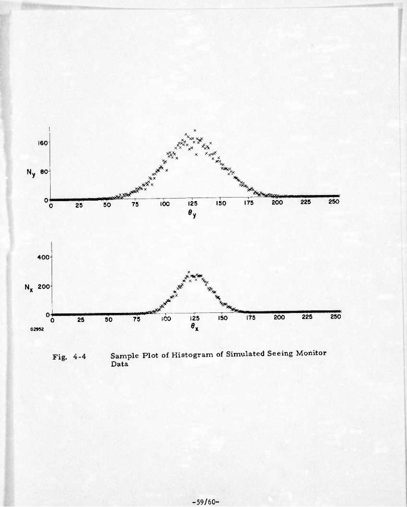
Because of the unavailability of field data, simulated data was generated to validate the processing software. The one second ,5ampleo of this data are shown in Fig. 4-2. The model used for this data was be. u on the visual interpretation of the analog records obtained from the SM c" -üng August 1975 (see Section 3). Arbitrary grey level units are used because of the existence of three different magnification ranges on the SM. After processing for one second samples the results are as shown in Fig, 4-3. In this simulation a definite linear trend was introduced in order to test this portion of the program. As discussed above, the length of the vertical lines indicate the variance in each 1000 member sample with the mean at the midpoint. After removal of this trend the histogram for ten seconds of data was generated This is shown in Fig. 4-4. These results are con- sistent with the Gaussian distribution of the initial random samples.

• 51.

READ 1 RECORD OFF TAPE (CONTAINS DATA FOR 1 SEC) REFORMAT THE WORDS; STORE SEEING ANGLES (fl ) ON DISK; COUNT NUMBER

I t = t + 1

NPTS, = NUM

ZERO THE N ARRAY I = 0

NO

I 1=1+1

I ■ NPTS

J = Ö (I) + 1

N(J) ■ N(J) + 1

YES

YES

NO

G2946

Fig. 4-la Flow Chart of Seeing Monitor Data Reduction Program

-52-

NO

! j = j +1

J = 256

JNJ = J ■ N(J) Kt= Kf+ JNJ

Lf =Lf + JNJ- J

YES

XBARt « (K, NPTSf)-l

SIGMA, = [L, (NPTSt-l) - (Kt NPTS,)2]

STORE N ARRAY AS A FUNCTION OF TIME

ALSO STORE K,, L,

YES ■♦( 100 j

]

NO

!

PLOT THE MEAN AND ERROR BARS FOR EACH SEC OF DATA

INPUT TJ, IF

(SECONDS)

G2949

LF =0

KF =0 NT^T = 0

I = -1 ZERO THE NSUM ARRAY V

Fig. 4-lb Flow Chart of Seeing Monitor Data Reduction Program

.53-

T = TI + I LF= LF+ L KF KF Kt

NT^ T = NT</) T + NPTS,

YFS

X = KF/NT^) T - 1

SIGMAX = [LF/(NT^ T -1)-(X + I.)2]

1= -1

NO

YES >

i r + i T= TI+I

READ (Nt (J), J = 1,256)

J= 0

1=1,

I NO J = J+l

J = 256 NSUM(J)= NSUM(J)+Nt (J)

YES

YES

G2950 ^

Fig. 4-lc Flow Chart of Seeing Monitor Data Reduction Program

■ 54.

! KF = 0 PF = 0 I ■ -1

][

r »

NO

1-1' 1 T = TI = I KR = KF = K, NPTS, PF = PF = K, NPTS, * t T. TF

YES

NS = TF - TI + 1

A = [2. (2 NS+ !)• KF-6. PFJ [NS- (NS- 1)

b = [12- PF - 6(NS + !)• KF] rNS-(NS- 1)(NS+ Dj

1 1

i.-.

t '

T = n= i TREND = A + B T- 128.5 READ (0t(K), K= 1, NPTS,)

J ■ 0

NO

J =■• J + 1 N(J) = 0 ru„

T::TF

MU J ■ 256

1 rYE S

K = 0

j K = K + 1 J = i (K)-TREND

, N (J) -- N (J) + 1 NO

K = NPTS

t , YE S

j.g

1 1 j = j + 1 1

NO ■j NSUM (J ■ NSUM(J)+ N(J) J =256 1;

x/c-r >" J

G2948

IYES

Fig. 4-Id Flow Chart of Seeing Monitor Data Reduction Program

■ 55-

WRITE THE SEEäHG ANGLES, RANGES, AND RETICLE WHEEL POSITIONS FOR THIS TIME INTERVAL ONTO A TAPE TO BE USED ON THE CDC 3174 FOR FURTHER ANALYSIS OF THIS DATA.

G2947

Fig. 4-le Flow Chart of Seeing Monitor Data Reduction Progra'

■56-

T=l SECOND

200

ey loo IMP

i 11

MMi • m mmi M0lia^m 200

Ö- 100 ,

100 200 300 400 500 600 700 800 900 1000 t(msec)

T=I0 SECONDS

200

fly 100

0 +

##^NtWW^

200

e loo #Ä^ 0 100 200 300 400 500 600 700 80C 900 1000

G295i t{msec)

Fig. 4-2 Sample Plot of Seeing Monitor Simulated Data

-57-

200

:iii,

Öy 100-

60 120

t (sec)

180

0

200'

100

G2953

0 + 0 60 120

t (sec)

180

Fig, 4-3 Display of One Second Averages of Raw Simulated Seeing Monitor Data with Error Bars

.58-

160

Ny 60]

25

,*& : >%$(

>fcx jy^x x

J^

50 75 100

X *&* X x

125 150 175 200 225 250

400

Nx 200

GZ952

# f$\

nwiiMiir y X

m 3h.

25 50 75 ICO 125 0v

150 MMpaai

175 200 225 mmmm 250

Fig. 4-4 Sample Plot of Histogram of Simulated Seeing Monitor Data

-59/60-

REFERENCES

1. Labeyrie, A., Astronomy and Astrophysics 6^, 85(1970).

2. Currie, D.C., Topical Meeting on Imaging in Astronomy, Cambridge, Mass. (1975).

3. Muller, R.A. and Buffington, A., J. Opt. Soc. Am. 64, 1200(1974).

4. Miller, L. Brown, W. P. , Jenney, J. A. and O'Meara, T.R. , OSA Topical Meeting on Optical Propagation through Turbulence, Boulder, Col. (1974).

5. Hardy, J.W., Feinleib, J. and Wyant, J.C., OSA Topical Meeting on Optical Propagation through Turbulence, Boulder, Col. (1974).

6. Yellin, M. , SPIE Symposium on Imaging through the Atmosphere, Reston, Virginia (1916).

7. Greenwood, D. P. and Youmans, D. B., RADC-TR-75-C-240 (Rome Air Development Center, Griffiss AFB, N. Y. , December 1975) (A019277).

8. Giuliano, C.R., et al. , Space Object Imaging. Final Report, Contract No. F30602-74-C-0227 (Rome Air Development Center, Griffiss AFB, N. Y.) , RADC-TR-76-54, (A023497).

9. Fried, D. L. , J. Opt. Soc. Am. 56, 1372 (1966).

10. Hall, F.F., Jr., in Temperature and Wind Structure Studies by Acoustic Echo Sounding, ed. by Derr, V.E., U.S. Govt. Pr. Off. 0322-0011 (1972).

11. Ochs, G.R., Wang, Ting-i and Lawrence, R.S., SPIE Symposium on Imaging through the Atmosphere, Reston, Virginia (1976).

12. Miller, M. G. and Kellen, P.P., RADC Tech. Report RADC-TR- 75-185 (Rome Air Development Center Griffiss AF Base, N. Y. July 1975) , (A015759).

13. Greenwood, D. P. et. al. , RADC Tech. Report RADC-TR-75-295 (Rome Air Development Center, Griffiss AFB, N, Y, , January 1976) (A021943).

14. Neff, W. D. , NOAA Tech. Report NOAA-TR-ERL-322-WPL-38 (NOAA Environmental Research Laboratories, Boulder, Colorado June 1975).

.-61-