Radar and LiDAR Fusion for Scaled Vehicle

Sensing

Gregory Beale

Thesis submitted to the faculty of the Virginia Polytechnic Institute and State University in partial

fulfillment of the requirements for the degree of

Master of Science

In

Engineering Mechanics

Miguel A. Perez, Chair

Zac R. Doerzaph

Matthew D. Berkemeier

February 23, 2021

Blacksburg, Virginia

Keywords: Sensor fusion, Kalman filter, Extended Kalman filter, Object tracking, Radar, LiDAR

All other material © by Gregory Beale

unless otherwise stated

Radar and LiDAR Fusion for Scaled Vehicle Sensing

Gregory Beale

ABSTRACT

Scaled test-beds (STBs) are popular tools to develop and physically test algorithms for advanced

driving systems, but often lack automotive-grade radars in their sensor suites. To overcome resolution

issues when using a radar at small scale, a high-level sensor fusion approach between the radar and

automotive-grade LiDAR was proposed. The sensor fusion approach was expected to leverage the higher

spatial resolution of the LiDAR effectively. First, multi object radar tracking software (RTS) was

developed to track a maneuvering full-scale vehicle using an extended Kalman filter (EKF) and the joint

probabilistic data association (JPDA). Second, a 1/5th scaled vehicle performed the same vehicle

maneuvers but scaled to approximately 1/5th the distance and speed. When taking the scaling factor into

consideration, the RTS’ positional error at small scale was, on average, over 5 times higher than in the

full-scale trials. Third, LiDAR object sensor tracks were generated for the small-scale trials using a

Velodyne PUCK LiDAR, a simplified point cloud clustering algorithm, and a second EKF

implementation. Lastly, the radar sensor tracks and LiDAR sensor tracks served as inputs to a high-level

track-to-track fuser for the small-scale trials. The fusion software used a third EKF implementation to

track fused objects between both sensors and demonstrated a 30% increase in positional accuracy for a

majority of the small-scale trials when compared to using just the radar or just the LiDAR to track the

vehicle. The proposed track fuser could be used to increase the accuracy of RTS algorithms when

operating in small scale and allow STBs to better incorporate automotive radars into their sensor suites.

Radar and LiDAR Fusion for Scaled Vehicle Sensing

Gregory Beale

GENERAL AUDIENCE ABSTRACT

Research and development platforms, often supported by robust prototypes, are essential for the

development, testing, and validation of automated driving functions. Thousands of hours of safety and

performance benchmarks must be met before any advanced driver assistance system (ADAS) is

considered production-ready. However, full-scale testbeds are expensive to build, labor-intensive to

design, and present inherent safety risks while testing. Scaled prototypes, developed to model system

design and vehicle behavior in targeted driving scenarios, can minimize these risks and expenses. Scaled

testbeds, more specifically, can improve the ease of safety testing future ADAS systems and help

visualize test results and system limitations, better than software simulations, to audiences with varying

technical backgrounds. However, these testbeds are not without limitation. Although small-scale vehicles

may accommodate similar on-board systems to its full-scale counterparts, as the vehicle scales down the

resolution from perception sensors decreases, especially from on board radars. With many automated

driving functions relying on radar object detection, the scaled vehicle must host radar sensors that function

appropriately at scale to support accurate vehicle and system behavior. However, traditional radar

technology is known to have limitations when operating in small-scale environments. Sensor fusion,

which is the process of merging data from multiple sensors, may offer a potential solution to this issue.

Consequently, a sensor fusion approach is presented that augments the angular resolution of radar data in

a scaled environment with a commercially available Light Detection and Ranging (LiDAR) system. With

this approach, object tracking software designed to operate in full-scaled vehicles with radars can operate

more accurately when used in a scaled environment. Using this improvement, small-scale system tests

could confidently and quickly be used to identify safety concerns in ADAS functions, leading to a faster

and safer product development cycle.

iv

Dedicated to my father. Role model and engineer.

v

Acknowledgements

First and foremost, I would like to thank my advisors, Dr. Perez, Dr. Doerzaph, and Dr.

Berkemeier. Their help has been instrumental over the last two and half years, and their expertise and

guidance have not only helped shape this work, but also shape me as an engineer and person. I would also

like to thank all of the colleagues at Continental Automotive and the Virginia Tech Transportation

Institute that have aided me in this project. The experiences I’ve gained working at Continental, for VTTI,

and on this study with the help of those mentioned have truly been invaluable.

Additionally, I want to thank my family and friends. Without their support I would not have been

able to overcome the challenges of the last three years, of which there were many. From my friends I have

learned so much about not only engineering, but also life as a whole during our time together. My parents

have always been the foundation on which I stand. I owe them everything and their love and support has

kept me centered when times were hard. To that I emphatically say, “Thank you.”

vi

Table of Contents

CHAPTER 1 – INTRODUCTION ................................................................................................................................. 1

CHAPTER 2 – LITERATURE REVIEW ...................................................................................................................... 2

2.1 RADAR SENSORS AND KALMAN FILTERING .................................................................................................... 2

2.2 LIDAR AND POINT CLOUD FILTERING .......................................................................................................... 10

2.2.1 DOWN SAMPLE PROCESS ............................................................................................................................. 12

2.2.2 GROUND PLANE ESTIMATION ...................................................................................................................... 13

2.2.3 CONVERTING CLUSTERS TO OBJECTS ........................................................................................................ 15

2.2.4 OBJECT TRACKING ....................................................................................................................................... 15

2.2.5 OBJECT CLASSIFICATION ............................................................................................................................ 16

2.3 SENSOR FUSION ............................................................................................................................................... 19

2.4 SCALED TEST BEDS ......................................................................................................................................... 24

2.5 CONCLUSION .................................................................................................................................................... 27

2.6 RESEARCH QUESTIONS ................................................................................................................................... 27

CHAPTER 3 – METHODS ........................................................................................................................................ 28

3.1 SENSOR IMPLEMENTATIONS AND TRIAL RUNS ............................................................................................. 28

3.2 RADAR TRACKING SOFTWARE ....................................................................................................................... 31

3.3 LIDAR CLUSTERING ......................................................................................................................................... 36

3.4 FUSION SOFTWARE .......................................................................................................................................... 37

3.5 ERROR METRICS ............................................................................................................................................. 39

CHAPTER 4 – RESULTS AND DISCUSSION ............................................................................................................. 42

4.1 FULL SCALE TESTS .......................................................................................................................................... 42

4.2 SMALL SCALE TESTS ....................................................................................................................................... 47

4.3 DISCUSSION ...................................................................................................................................................... 52

4.3.1 FULL-SCALED TESTS .................................................................................................................................... 52

4.3.2 SMALL-SCALED TESTS.................................................................................................................................. 54

4.3.2.1 RADAR AND LIDAR ERROR METRIC COMPARISONS ............................................................................. 54

4.3.2.2 FUSION TRACK METRICS .......................................................................................................................... 55

CHAPTER 5 – CONCLUSIONS ................................................................................................................................. 58

5.1 LIMITATIONS.................................................................................................................................................... 59

5.2 FUTURE WORK ................................................................................................................................................ 59

REFERENCES .......................................................................................................................................................... 60

vii

APPENDIX A ........................................................................................................................................................... 63

SMALL SCALE “STRAIGHT” TRIAL RUN GRAPHS ................................................................................................ 63

APPENDIX B ........................................................................................................................................................... 66

SMALL SCALE “DIAGONAL” TRIAL RUN GRAPHS ............................................................................................... 66

APPENDIX C ........................................................................................................................................................... 69

SMALL SCALE “S-TURN” TRIAL RUN GRAPHS ..................................................................................................... 69

APPENDIX D ........................................................................................................................................................... 72

CONTINENTAL AUTOMOTIVE ARS 400 SERIES RADAR DATA SHEET ............................................................... 72

APPENDIX E ........................................................................................................................................................... 74

VELODYNE PUCK LIDAR DATA SHEET ............................................................................................................. 74

1

CHAPTER 1 – INTRODUCTION

This study aims to generate a fusion technique that uses radar and Light Detection and Ranging

(LiDAR) sensor inputs to improve radar tracking performance in a small-scaled vehicle testbed. Scaled

testbeds (STBs) derive value from accurately modeling full-scale system behavior within existing physical

constraints while requiring minimal changes in control software functionality. Currently, vehicular STBs

largely lack the ability to accommodate radars due to sensor scaling issues. In a small-scaled environment,

the incoming radar data cannot provide the same spatial resolution that would normally be found in full-

scale tests, resulting in less radar returns per object, more sensor noise, and, thus, poorer object tracking

over time.

One solution to this issue is to modify the underlying tracking algorithm to perform optimally in

the scaled environment. However, this would gravely decrease the value of the small-scale tests as the

algorithm would significantly change between small-scale testing and the implementation of its full-scale

counterpart. This manipulation would make test results difficult, if not impossible, to compare.

The proposed solution is to augment the traditional radar data returns in the small-scale

environment with LiDAR. These sensors, while expensive and susceptible to noise in some environments,

have much higher spatial resolutions than typical automotive radar sensors can achieve. Therefore, the

LiDAR point cloud information could theoretically be used, through a sensor fusion approach, to augment

depleted radar returns from an object in a small-scaled environment. A track-to-track fusion technique

could be used between the two sensors to help the radar better estimate the position and trajectory of the

object or vehicle being tracked within the small-scale environment.

In this investigation, software techniques from four fields of study were assessed to accomplish

this goal: 1) Kalman filtering for automotive radars, 2) point cloud filtering with LiDARs, 3) sensor fusion

techniques, and 4) small-scaled vehicle implementations. Each of these fields has been the subject of

much recent attention as automated driving functions have holistically improved, but there is a large gap

in the research when it comes to utilizing software solutions developed at full-scale to function with

STBs. This study seeks to offer a potential solution to bridge that gap.

The initial step undertaken was to review previous work in these fields, documented in the form of

a literature review. The review contains four main sections: Radar sensors and Kalman filtering; LiDAR

point cloud filtering; sensor fusion; and scaled testbeds. The knowledge obtained from this systematic

review was used to develop an efficient and effective fusion approach and to guide the acquisition of

empirical data. In turn, the empirical data was used to 1) quantify the extent to which a reduction in

environment scale reduced the accuracy and resolution in radar returns and 2) verify and quantify the

extent to which the proposed fusion approach could generate trajectory data that properly simulated full-

scale vehicle returns within the scaled environment.

2

CHAPTER 2 – LITERATURE REVIEW

2.1 RADAR SENSORS AND KALMAN FILTERING

Radar detects objects within its field of view (FOV) by transmitting and receiving electromagnetic

waves. A radar can report each object’s position, radial velocity relative to the sensor, and an estimated

radar-cross sectional (RCS) area. Engineers began working on automotive-grade radar in the 1970s due to

its potential crash prevention applications. An early application of vehicle-mounted radars occurred on

Greyhound buses in 1992, aimed at alerting bus drivers to impending forward collisions [1]. A subsequent

application by Bosch, circa 1998, provided adaptive cruise control (ACC) functionality for Mercedes S-

class sedans, and resulted in the first commercially available automotive radar system [1]. Since then,

radars have increasingly become the pivotal sensor used to attain advanced driver assistance system

(ADAS) functionalities. ADAS functions such as ACC, blind spot detection, forward collision warning,

rear cross traffic alert, and advanced emergency truck braking systems heavily depend on radar sensors.

Automotive radars operate in two frequency bands, 24 GHz and 77 GHz, corresponding to 12 mm

and 4 mm wavelengths, respectively, and are highly compact while being energy and computationally

efficient. Each radar cycle results in a list of detection points that the radar can consolidate into data return

values (i.e., radar “clusters”). In automotive radar, each cluster has four associated characteristics: lateral

and longitudinal distance from the sensor (although radars do not inherently report clusters in the typical

x-y coordinate scheme, but instead do so in the polar coordinate system – a non-linear coordinate

transformation is required to convert to Cartesian coordinates), velocity radial to the sensor, and RCS. A

typical radar cycle can detect anywhere between 10 and 75 clusters depending on the radar’s software

limits and the complexity of the environment [47]. Modern long-range radar sensors, such as a

Continental ARS408, split their FOV into a long-range scan and a near-range scan to support multi-

purpose use. Reported statistics of the typical ARS408 can be found in Table 1 [2]. Operating at

approximately 14 Hz (72 ms period), the ARS408 radar can report clusters at varying radial velocity,

angle, and distance resolutions depending on their location in the near and far scans. The full spec sheet

can be found in Appendix D.

Table 1:ARS408 Long Range Radar Sensor data sheet excerpt

Measuring Performance Comment To natural targets (non-reflector targets

Distance range

0.20 ...250 m far range,

0.20...70m/100m@0…±45° near range and

0.20…20m@±60° near range

Resolution distance measuring point targets, not tracking Up to 1.79 m far range, 0.39 m near range

Accuracy distance measuring point targets, not tracking ±0.40 m far range, ±0.10 m near range

Azimuth angle augmentation (field of view FoV) -9.0°...+9.0° far range, -60°...+60° near range

3

Elevation angle augmentation (field of view FoV) 14° far range, 20° near range

Azimuth beam width (3 dB) 2.2° far range,

4.4°@0° / 6.2°@±45° / 17°@±60° near range

Resolution azimuth angle point targets, not tracking 31.6° far range,

3.2°@0° / 4.5°@±45° / 12.3°@±60° near range

Accuracy azimuth angle point targets, not tracking ±0.1° far range, ±0.3°@0°/ ±1°@±45°/

±5°@±60°near range

Velocity range -400 km/h...+200 km/h (- leaving

objects...+approximation)

Velocity resolution target separation ability 0.37 km/h far field, 0.43 km/h near range

Velocity accuracy point targets ±0.1 km/h

Cycle time app. 72 ms near and far measurement

Antenna channels /-principle microstripe

4TX/2x6RX = 24 channels = 2TX/6RX far -

2TX/6RX near /

Digital Beam Forming

Several key signal processing and electrical engineering tools and techniques are needed in

modern radars [3]. For example, radar chirps, frequency modulated continuous-wave (FMCW)

transmitters, fast Fourier transforms (FFTs), and specialized antenna arrays allow radars to continuously

transmit (Tx) and receive (Rx) signals and then convert the returns into the aforementioned four

dimensions reported for return signal clusters. In fact, the resolution of the velocity, range, and angle

measures are limited by the FFTs performed in the sensor, which are inherently discrete in nature.

Algorithms exist to provide additional resolution in those fields. These algorithms, however, tend to be

complex and computationally expensive, so they are rarely used in commercial radars [3].

There is substantial literature dedicated to signal processing techniques and their implementation

in radars. That literature is not considered herein, given that this investigation will use a commercially

available radar that already incorporates industry-standard practices. Instead, the investigation aims to

consider only the reported clusters from the commercially available sensor and attempt to minimize the

diminished tracking abilities of the radar when it is operated at small-scale. For the interested reader,

Patole, et al. (2017) provide an excellent overview of these techniques and describe a number of radar-

applicable signal processing resources [3].

Radars excel at collecting real-time data from a dynamic environment but need filtering and

estimation techniques to translate radar clusters into object tracks over time. This is generally true for any

active perception sensor. Optimal state estimation, which tracking filters generally attempt, is a classic

control theory problem with abundant literature. Early research in this field combined statistics to address

one of the most important problems of the time: accurately estimating the state of a process in the

presence of random noise – ever more important as electrical sensors became increasingly popular. This is

the problem area where, in 1960, R. E. Kalman published his seminal work “A New Approach to Linear

Filtering and Prediction Problems” and first introduced the famous Kalman filter (KF) [4].

4

Originally a project for the Department of Defense, Kalman was attempting to estimate the state of

a linear time discrete system under both control and observation and developed a recursive software

solution that “minimized the mean squared error of that process” [4]. In this case, “control” specifically

refers to the ability to provide input commands to the system, while recording measurements from the

system falls under “observation.” Many systems are both controlled and observed, although, in the case of

radar object tracking, the system (i.e., other vehicle) will be under observation but not control. The basis

for the filter is a linear predict-update model able to recursively include all past data in the state estimation

without the need to continually store it. This greatly simplified the mathematics and computational

requirements for filtering problems – something particularly relevant for processing occurring within

embedded systems. The literature surrounding KF implementations is vast. The subsequent discussion is

therefore focused on a high-level overview of the KF process and the variations of the KF that are

common in automotive radars, such as the extended Kalman filter (EKF) and data association models.

In a KF, the noise in the system is often modeled as a Gaussian (normal) distribution with a mean

value of zero and some variance value, σ2. Due to this noise, the accuracy of the underlying system cannot

be fully trusted, and the reported measurement is considered a combination of the true value skewed by

some amount of unknown random noise. Therefore, the true state value is modeled as Gaussian

distribution over the state space with inherent standard deviation [4]. By modeling the noise, the system

estimate provided by a KF can, given the known added biases of the sensor(s), seek the true state value

instead of erratically jumping in a non-smoothed or “unfiltered” way between the reported values.

At the heart of the KF’s predict and update model are Bayesian statistics, specifically Bayes

theorem. Summarized in this context, the theorem concludes that given some knowledge about the current

state of a system or process (expressed as a probability or underlying variance), it is more accurate to first,

predict the state of the system in the future based off the current estimate and then, second, update that

predicted state based on incoming noisy measurements; than it is to only update the state based on the

measurements alone [5]. In this sense, all probabilistic information about a system can be helpful and

should be included. No matter how uncertain one can be about a measurement’s true accuracy, the

information it provides still contributes to improve the overall tracking accuracy [6].

Consequently, there are two major sets of linear control equations included in a KF. One pertains

to the prediction update (a priori estimate) and the other to the measurement update (a posteriori

estimate) [5].

The prediction step requires three basic elements: 1) the magnitude of the time step used to predict

the future state, 2) the process noise expressed in variances and covariances (i.e. uncertainty values in the

model predictions), and 3) the current covariances of the system. Only two calculations are needed. One

calculation predicts the state at the future time step (Eqn. 1), and one updates the covariances of the

system given the process noise (Eqn. 2).

Similarly, the measurement update requires three elements: 1) a matrix to map the measurement to

the state space, 2) the sensor noise expressed in variances and covariances, and 3) the measurement values

themselves. Three equations are then computed to complete this step of the KF. First, the Kalman gain is

computed with knowledge of the sensor noise and the previously updated covariance matrix from the

predict step (Eqn. 3). The Kalman gain is used as a weighting factor in whether to trust the a priori

estimate of the current state more or less than the incoming measurement values and, thus, introduces

5

Kalman’s novel approach to the filtering problem [4]. Second, the a posteriori state estimate is calculated

using the Kalman gain factor along with the difference between the predicted and measured (from the

sensors) states (Eqn. 4). Third, the covariance matrix of the system is updated to express the filter

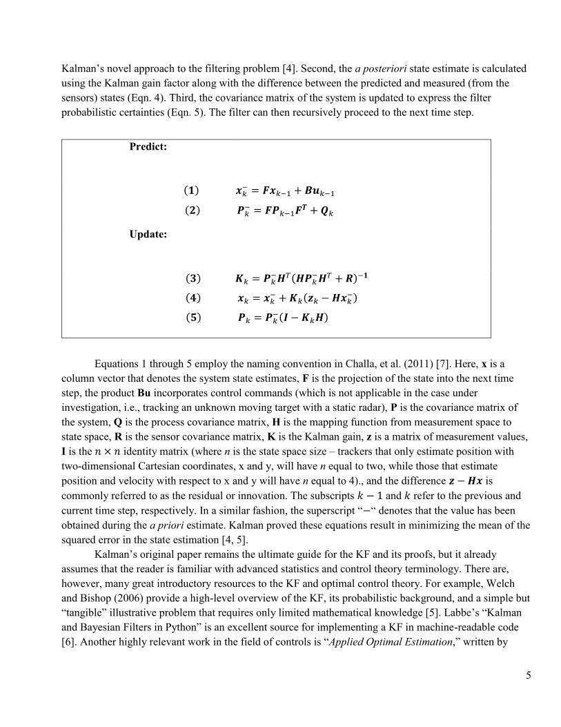
probabilistic certainties (Eqn. 5). The filter can then recursively proceed to the next time step.

Predict:

(𝟏) 𝒙𝑘− = 𝑭𝒙𝑘−1 + 𝑩𝒖𝑘−1

(𝟐) 𝑷𝑘− = 𝑭𝑷𝑘−1𝑭

𝑻 + 𝑸𝑘

Update:

(𝟑) 𝑲𝑘 = 𝑷𝑘−𝑯𝑇(𝑯𝑷𝑘

−𝑯𝑇 + 𝑹)−𝟏

(𝟒) 𝒙𝑘 = 𝒙𝑘− + 𝑲𝑘(𝒛𝑘 − 𝑯𝒙𝑘

−)

(𝟓) 𝑷𝑘 = 𝑷𝑘−(𝑰 − 𝑲𝑘𝑯)

Equations 1 through 5 employ the naming convention in Challa, et al. (2011) [7]. Here, x is a

column vector that denotes the system state estimates, F is the projection of the state into the next time

step, the product Bu incorporates control commands (which is not applicable in the case under

investigation, i.e., tracking an unknown moving target with a static radar), P is the covariance matrix of

the system, Q is the process covariance matrix, H is the mapping function from measurement space to

state space, R is the sensor covariance matrix, K is the Kalman gain, z is a matrix of measurement values,

I is the 𝑛 × 𝑛 identity matrix (where n is the state space size – trackers that only estimate position with

two-dimensional Cartesian coordinates, x and y, will have n equal to two, while those that estimate

position and velocity with respect to x and y will have n equal to 4)., and the difference 𝒛 − 𝑯𝒙 is

commonly referred to as the residual or innovation. The subscripts 𝑘 − 1 and 𝑘 refer to the previous and

current time step, respectively. In a similar fashion, the superscript “−“ denotes that the value has been

obtained during the a priori estimate. Kalman proved these equations result in minimizing the mean of the

squared error in the state estimation [4, 5].

Kalman’s original paper remains the ultimate guide for the KF and its proofs, but it already

assumes that the reader is familiar with advanced statistics and control theory terminology. There are,

however, many great introductory resources to the KF and optimal control theory. For example, Welch

and Bishop (2006) provide a high-level overview of the KF, its probabilistic background, and a simple but

“tangible” illustrative problem that requires only limited mathematical knowledge [5]. Labbe’s “Kalman

and Bayesian Filters in Python” is an excellent source for implementing a KF in machine-readable code

[6]. Another highly relevant work in the field of controls is “Applied Optimal Estimation,” written by

6

Gelb et al. (1974) [8]. A more modern book about controls and filtering is presented by Stengel in

“Optical Control and Estimation” (1994) [9].

Since Stengel’s book in 1994, and as interest in automated driving has grown, publications focused

on the software implications of tracking and filtering techniques have become more prevalent. Bar-

Shalom et al. (2001) published “Estimation with Applications to Tracking and Navigation” which

provides an extensive overview on the theory and computational algorithms for estimation. Bar Shalom et

al. (2001) particularly discusses the design and evaluation of state estimation algorithms that operate in a

stochastic environment [10]. These algorithms form the backbone of information extraction systems for

the remote sensing of moving objects, which are highly useful for automated driving. More recently,

Challa et al. (2011) have discussed tracking solutions in their book “Fundamentals of Object Tracking”

[7]. Challa et al. (2011) particularly provide an excellent source of knowledge on radar cluster tracking as

many iterations of pseudo-code are provided. Due to their comprehensive discussion of approachable but

thorough techniques for tracking and filtering, both works from Challa et al. (2011) and Bar-Shalom et al.

(2001) are widely used by industry experts today.

Radar trackers used in industry rely heavily on the “base” KF. However, there are unique nuances

in radar tracking, particularly in the automotive environment, that require additional elaboration on the KF

method. Thus, there are two important additional facets of Kalman filtering for automotive radars: the

extended Kalman filter (EKF) variation and the data association problem.

The extended Kalman filter variation arises from the origin of the KF – while Kalman originally

designed the KF to track linear processes, purely linear applications are rarely observed in nature.

Vehicles, airplanes, pedestrians, and other objects of interest can easily accelerate in two or three

dimensions and linear models are often inadequate to effectively track their movement. This required a

solution for non-linear tracking with the KF, which became the extended Kalman filter. Based on the

popular technique to linearize any non-linearities in the model by using the first few terms in a Taylor

Series expansion, the EKF uses partial derivatives of the process and measurement relationships with

respect to the state vector to predict the system state [5]. Systems governed by non-linear equations are

accompanied by continuously changing values for the sensor and process covariance matrices (R and Q,

respectively), and the mapping matrix (H). To combat this, at each time step, the Jacobian of those

matrices is computed and applied to the covariance matrices. Additionally, the nonlinear functions for the

time projection (f) and mapping (h) can be defined for each time step to take into account any non-linear

movement in the state or non-linear mappings of the state space to the measurement space. Welch and

Bishop (2006) provide a good overview of this process and the variation of the five KF equations

required, which are presented in Equations 6 to 10 [5, 11].

Predict:

(𝟔) 𝒙𝑘− = 𝒇(𝒙𝑘−1, 𝒖𝑘−1)

(𝟕) 𝑷𝑘− = 𝑭𝑷𝑘−1𝑭

𝑻 + 𝑾𝑘𝑸𝑘−1𝑾𝑘𝑻

Update:

(𝟖) 𝑲𝑘 = 𝑷𝑘−𝑯𝑘

𝑻(𝑯𝑘𝑷𝑘−𝑯𝑘

𝑻 + 𝑽𝑘𝑹𝑘𝑽𝑘𝑻)

−𝟏

7

(𝟗) 𝒙𝑘 = 𝒙𝑘− + 𝑲𝑘(𝒛𝑘 − ℎ(𝒙𝑘

−))

(𝟏𝟎) 𝑷𝑘 = 𝑷𝑘−(𝑰 − 𝑲𝑘𝑯𝑘)

The terms of Wk, Vk, and Hk have been added to represent the Jacobian at time step k of the

process covariance matrix, the sensor noise covariance matrix, and the mapping function, respectively.

The most important step in the EKF process relies on linearizing the mapping function, H, as it relates

non-linear system measurements to linear estimates, h(), that fit within the linear stochastic model of the

KF. Each of the three measurement update equations (Eqns. 8, 9, 10) rely on the linearization of the

mapping function [6]. Systems that attempt to model the changing velocity of tracked objects need to

expand this step from the regular KF to the EKF. All books referenced earlier (i.e., Welch and Bishop,

Gelb et al., Stengel, Bar-Shalom et al., and Challa et al.) dedicate extensive discussion to the EKF because

of its wide range of applications and importance.

Although the EKF can be applied to many non-linear tracking problems, Bizup et al. (2003) have

argued that complete linearization in the mapping function, H, results in an “over-extended” Kalman filter

that may actually introduce errors over time [11]. Bizup et al. (2003) propose that, for tracking systems

that measure range, angle, and – most importantly for radars – range rate, it is more accurate to

“alternatively” linearize the mapping matrix so that the range rate is only related to the velocity estimates.

Originally, the linearization of the mapping function results in position and velocity estimates that are

functionally related to the range rate, causing unnecessary convolution. Bizup et al. (2003) simplify this

linearization into the “aEKF” (alternative EKF) and show it results in quicker convergence for filters that

incorporate range rate measurements. This approach has been adopted by some industry-developed

automotive radar trackers.

The second required extension of the KF for automotive applications relates to the data association

problem. Given that many perception sensors return multiple values per cycle (e.g., radar), these data

returns need to be associated with objects in the environment before they can be passed into a Kalman

filter. If there are multiple objects within the sensing area, the data from one object should not be

conflated with the data return from another object, since this would clearly result in erroneous and

unusable tracking solutions from the KF. In fact, out of all the factors influencing the KF, correct

implementation of data association techniques can have the most influence on filter accuracy [7]. As a

result, several different models have been developed to implement data association techniques.

The first step in successful data association is to create multi-track capability within the software

program tracking the data measurements. In this manner, a set number of environmental objects can be

observed and tracked over time, which is extremely imperative for automotive or robotic uses in

uncontrolled environments. Multi-track KFs require the addition of an object list – each running their own

KF – and some version of a data association technique to match the data returns to specific objects (or

create new ones where necessary). A basic association technique is the nearest neighbor filter (NNF). In

simplified tracking environments where an object only returns a single data return to the sensor, the NNF

first filters all the data returns to a statistically relevant area around the tracked object (a process called

gating) and then selects the closest measurement to the predicted state of the tracked object. All other data

returns are considered extraneous and the result of sensor noise and unwanted clutter inherent in the

8

environment [7]. Because the state covariance matrix includes standard deviation information, the point-

by-point statistical comparison to find, first, the gating thresholds, and then, the closest data point is

relatively straightforward, and the closest point can be easily selected. As described, the NNF limits its

state update equations to a single data point, which, in actual tracking applications may not be as useful

considering multiple data points can originate from the same object of interest. The simplified NNF

therefore discards many of these useful data points.

The probabilistic data association filter (PDA) and its variations, on the other hand, use all the

gated data returns to update the state prediction and are generally accepted as more accurate than the NNF

in complex tracking environments. The PDA filter, however, requires two assumptions: 1) in the

simplified tracking environment, the object of interest only results in one true data return to the sensor,

and 2) the extraneous data returns are uniformly distributed in the perception space [7]. Following these

assumptions for the PDA, the true measurement of the object lies somewhere within the gated threshold

values but cannot be exactly determined by selecting only one of the gated measurements. Instead, the

PDA filter proposes to use all gated measurements after they are statistically weighted, and their

probabilities normalized [10]. In this manner, data points that more closely resemble the predicted state

account for more in the measurement update step, but other returns within statistically relevant positions

in the environment still influence the a posteriori state estimate.

One particular adaption of the PDA is the joint probabilistic data association (JPDA) filter. This

extends the underlying principles of the PDA filters to work well when multiple tracks cross within close

proximity – a scenario where the accuracy of the NNF and basic PDA filters often suffers due to their core

assumptions, specifically the PDA assumption of uniform distribution of extraneous data returns outlined

above. When track validation gates overlap, measurements from sensors can fall within both gates (Fig.

1). For example, it is not immediately clear which track the measurement M3 belongs to. The NNF will

choose the closest points to the center of the tracks, assuming all others to be possible new tracks; the

PDA filters will weigh all measurements in the validation gate based on statistical proximity and expected

noise densities in the viewing area. For PDA filters, this can cause errors in measurement probability

weightings when those measurements actually originate from another track and are not sensor noise, and,

possibly, the tracker could diverge [50]. Fortmann et al. (including Bar-Shalom) recognized this limitation

of PDA filters and proposed their solution: the JPDA.

Figure 1: Typical data association problem with 2 tracks and 4 measurements and associated validation gates

9

To overcome this issue, Fortmann et al. (1983) modify the way probabilistic weightings were

calculated using what they called “feasible joint events.” This time, the JPDA can probabilistically weigh

the shared measurements of validation gates as possibly coming from both tracks and not as strictly noise

like the PDA does. For every instance that track validation gates overlap, a cluster is extracted and a

binary validation matrix is created (Fig. 2). This matrix outlines the measurement and track possible

pairings: each row is a measurement, and each column is a track assignment with the first column

representing clutter. Values of “1” signal a possible pairing and values of “0” indicate non-possible

pairings based on the validation gates. Of course, measurements outside the gates are not included. From

here, “feasible joint events” – possible measurement and track pairing combinations – are created and

commonly labeled Ωi [50]. Feasible events are created by looping through the validation matrix and

selecting one measurement per row and one track per column. This ensures that the measurement could

only come from one source, and each track is associated with only on measurement (the noise column can

have any number of measurements because the JPDA needs to be able to model the situation where all

measurements were the result of clutter) [50]. The validation matrix and collection of feasible events for

the instance in Fig. 1 is shown in Fig. 2.

Figure 2: Validation and feasible event matrices for the configuration in Fig. 1 [51]

The feasible joint event matrices allow the JPDA to calculate the correct association probabilities

denoted 𝛽𝑚𝑡 , where t is the track number and m is the measurement number. Calculating 𝛽𝑚

𝑡 is analogous

to calculating the probability that the measurement, m, belongs to the track, t [50]. Using the expected

probability of detection for the track, whether the measurement was assigned to a track or clutter, the

probability density for each measurement and track pair, and a normal distribution scaled by the

innovation, probabilities for each element of the feasible event matrices are calculated. Then, the

probabilities for each measurement and track pair in the validation matrix can be summed by the

corresponding entries in Ωi and normalized to arrive at 𝛽𝑚𝑡 , the correct weighting factors for the JPDA

[51]. The probabilities 𝛽𝑚𝑡 influence the overall innovation matrix for the measurements in this timestamp

and, in the immediate steps, the Kalman gain factor.

10

Fortmann et al. (1983) successfully demonstrated the JPDA’s superiority over the regular PDA

and the NNF when tracking crossing targets in the presence of clutter using their technique. However, the

JPDA can suffer from long run times based on the sheer number of feasible event matrices needed and

high volume of probability calculations for each of those matrices. The example in Fig. 1 only contained 3

measurement points and 2 overlapping tracks, but those instances where more tracks overlap or there are

more measurements (possibly from multiple sensors) can result in millions of feasible event matrices [51].

Important contributions have been made to improve calculation times while maintaining accuracy. Fisher

and Casasent (1989) propose using vector inner products and a modified analog validation matrix to

reduce the number of calculations, although it requires a specialized optical processor [51]. Efficient

depth-first searches have also been proposed to populate measurement and target pairs, thus speeding up

probability coefficient calculations [52]. Quick approximation methods for the 𝛽𝑚𝑡 values have also been

shown to greatly improve calculation times when only 3 or less track validation gates overlap at any given

time [52]. Musicki and Evans (2002) implement an integrated JPDA that focuses on track existence

probabilities, paving the way for the trackers to tentatively create new tracks, confirm tentative tracks, and

delete old tracks all based on track existence and the data associations made by the JPDA [53]. All

modern JPDA trackers implement the original JPDA proposed by Fortmann et al. (1983) with some form

of improvements in approximation made by the likes of [51, 52, 53]. The work in this project will draw

heavily from implementations of both the NNF and JPDA.

In addition to [51, 52, 53], both Challa et al. (2011) and Bar-Shalom et al. (2001) describe the

probabilistic mathematics that underlie such algorithms.

2.2 LIDAR AND POINT CLOUD FILTERING

LiDAR is a time of flight sensor technique that uses projected infrared lasers (~900 nm

wavelength) to map the surrounding environment. Originally used for geographic mapping, the approach

has been adapted to automotive use, particularly as autonomous driving systems have increased. Given

that a single return pulse from one of these lasers can provide a distance value for one object, modern

LiDAR systems typically incorporate multiple fast pulsing lasers in a mechanically spinning sensor to

achieve a full 360° horizontal FOV. The different lasers, often called channels, are differentially angled to

ensure complete coverage of a defined vertical FOV, often 30° or more. As the sensor spins, the lasers

continually pulse at nearly 1000 Hz to collect data returns. With cycle times as high as 20 Hz, modern

LiDAR systems can report hundreds of thousands and even millions of data points per second depending

on how many channels they feature (the maximum number of channels available in a production LiDAR

system is currently 128). Four characteristics can be derived from a single data return: distance values in

the longitudinal (x), lateral (y), and vertical (z) directions, and an intensity value of the return. While both

radars and LiDARs can detect obstacle position, LiDARs lack the ability to determine the range rate of an

object in its FOV. However, a tradeoff between the volume of data and range rate reporting exists

between the two sensors: although the radar can report radial velocity for each return, the LiDAR sensor is

able to sense the world at a higher resolution.

In this investigation, a 16 channel Velodyne PUCK LiDAR will be used to support the sensor

fusion task. This LiDAR unit, which is currently the more cost-effective sensor offered by Velodyne,

11

features a 360° horizontal FOV, 16 laser channels, a range up 100 meters, +/- 3 cm accuracy, 30° vertical

FOV, horizontal angle resolution of 0.1° – 0.4°, operating speed of 5 – 20 Hz, 905 nm operating

wavelength, microsecond data timestamping, and a collection rate of up to 300,000 points per second

[12]. The full data sheet for the PUCK LiDAR is available in Appendix E.

The most basic way to visualize LiDAR data points is in a point cloud. The x, y, and z components

of each data return can be easily visualized at each frame, and the sheer volume of points reported by the

sensor allows the presentation of an intuitive map of the surrounding area to the human viewer. A typical

point cloud visualization is shown in Figure 3. The color of each dot is directly related to the intensity of

the return – red denotes strong returns, while yellow and green points denote progressively weaker

returns. Each point cloud often contains one complete rotation of the sensor and all the data points

contained therein. Therefore, the sensor essentially builds a snapshot of the environment from the

perspective of the sensor itself.

Figure 3: LiDAR point cloud

With hundreds of thousands of incoming points per second, efficient ways to store and process

LiDAR data are essential. Many software solutions have been proposed for specialized projects, but

currently one popular option is the open source point cloud library (pcl). Supported by corporations such

as Google, Intel, Toyota, Velodyne, Nvidia, and Willow Garage; and many academic institutions, pcl is a

cross-platform framework written and implemented in C++ that offers software solutions for the storage

and processing of point cloud data from a variety of sensors, including camera and LiDAR [13]. The

libraries in the framework incorporate many of the modern point cloud filtering and processing techniques

that will be discussed later in this review and, with pcl’s in depth tutorials, can be implemented into a

wide range of solutions. Pcl attempts to provide a mainstream framework and code repository for industry

partners and researchers alike, allowing for the easier implementation and understanding of developed

point cloud filtering solutions. This aim makes it popular for use in robotic prototyping and autonomous

driving systems, which has resulted in the development of a pcl plug-in for the prominent Robot

Operating System (ROS) framework.

LiDARs are excellent at delivering high-spatial resolution data of the world that surrounds the

sensor, but significant point cloud processing and filtering is needed to convert those data into useful

information. A large body of research has been devoted to the development of these algorithms,

12

particularly since the birth of autonomous driving systems in the early 2000s. For autonomous driving

systems using LiDARs to work, embedded hardware and software – either in the LiDAR or in the vehicle

– must be able to perform at least a subset of several critical tasks with the incoming point cloud data.

These include estimating the drivable road area, identifying traffic objects (e.g., pedestrians, cyclists,

other vehicles), classifying other environmental objects (e.g., buildings, fences, guardrails, lane lines, stop

signs, trees), and performing object tracking. The correct classification of areas within the point cloud

allows the vehicle to build a real-time map, localize, and path plan as the vehicle navigates the road.

Therefore, the need for efficient data association techniques for automotive-grade LiDARs is evident.

Currently, no single algorithm can provide end-to-end filtering and classification capabilities in the

automotive domain. Effective LiDAR systems incorporate multiple techniques to process a single point

cloud. An overview of a typical automotive LiDAR system includes algorithms designed to:

1) Down-sample the original point cloud into clusters, voxels [48], occupancy grids, or octrees [16] to reduce

computational processing time;

2) Estimate the drivable area using RANSAC (i.e., random sample and consensus [19]) or another ground

plane estimator;

3) Convert clusters to objects and systematically assign data points to those objects, using a density or nearest

neighbor approach;

4) Track objects over time using Kalman filter or other similar technique to identify dynamic and static

obstacle tracks; and

5) Classify an object based on pre-specified parameters relative to the application and environment.

Research in this field was originally focused on the development of each of these individual steps, but

more recent efforts have focused on the efficient implementations of these algorithms for the system as a

whole to achieve near real-time sensing. Additional discussion on each of these steps is provided in

subsequent subsections.

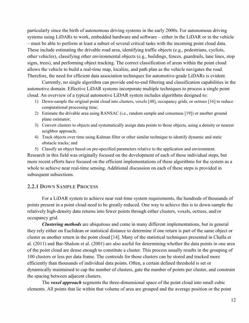
2.2.1 DOWN SAMPLE PROCESS

For a LiDAR system to achieve near real-time system requirements, the hundreds of thousands of

points present in a point cloud need to be greatly reduced. One way to achieve this is to down-sample the

relatively high-density data returns into fewer points through either clusters, voxels, octrees, and/or

occupancy grid.

Clustering methods are ubiquitous and come in many different implementations, but in general

they rely either on Euclidean or statistical distance to determine if one return is part of the same object or

cluster as another return in the point cloud [14]. Many of the statistical techniques presented in Challa et

al. (2011) and Bar-Shalom et al. (2001) are also useful for determining whether the data points in one area

of the point cloud are dense enough to constitute a cluster. This process usually results in the grouping of

100 clusters or less per data frame. The centroids for those clusters can be stored and tracked more

efficiently than thousands of individual data points. Often, a certain defined threshold is set or

dynamically maintained to cap the number of clusters, gate the number of points per cluster, and constrain

the spacing between adjacent clusters.

The voxel approach segments the three-dimensional space of the point cloud into small cubic

elements. All points that lie within that volume of area are grouped and the average position or the point

13

closest to the average position is often returned as the single data point for that voxel [15]. The data within

the point cloud is then reduced to the number of voxels, which are often several orders of magnitude less

than the original number of points.

The octree is an extension of the voxel approach. As the name suggests, octrees are hierarchical

tree data structures where each node has eight leaves. The root of the tree stores the averaged data

centroid for that voxel space, where each child level divides the space into eight octants and keeps track of

any averaged centroids that were computed [16]. In this way each octree root node can average

information from a high number of clustered points, depending on the size of the voxels. Each level of the

octree increases the resolution – 64 smaller voxels can be stored with an octree height of 4, including the

root node. More resolutions are available at the price of computational time. Fig. 4 shows a common

octree visualization from free space to hierarchical data tree [54].

Figure 4: The breakdown of volumetric space into an octree [54]

Occupancy grids project the three-dimensional point cloud into a two-dimensional grid where

points are commonly stored in lists based on their height (z-coordinate) in the point cloud space [17].

Clustering based on height or proximity can then be done for each grid block, reducing complexity. For

algorithms that utilize occupancy grids, height maps are frequently involved. Clustering is often done after

the down-sampling process is complete for computational efficiency.

2.2.2 GROUND PLANE ESTIMATION

Because automotive LiDARs are deployed in areas where driving is possible, a large percentage of

the data points within the point cloud originate from the road surface. Algorithms that can detect the road

surface within point cloud data fall under the general category of plane estimators. The correct

identification of this “ground” plane benefits the system in two major ways. First, the data points that

constitute the ground plane can be removed from the point cloud once identified. There is no need to pass

this data to any clustering methods since the road pavement itself is not, in most applications, considered

an object that the system should avoid. The resultant reduction in data points increases computational

efficiency. Second, the height of the ground plane can be used as a gate to identify other environmental

objects. All road objects such as curbs, other vehicles, pedestrians, and cyclists should have data returns

that originate with z-values and centroids that are located above the road. Similarly, suspended objects

such as bridges, traffic lights, and overhanging signs should have heights substantially above the road

14

surface level. A direct comparison between the height of the estimated ground plane and the height of a

cluster can therefore be used to determine certain classification levels for an object [18].

There are many ground plane estimation techniques that range from simple (e.g., linear regression,

height cut-offs) to highly complex (e.g., Markov models). The simplest method involves cutting off all

points below a certain height value, usually informed by the placement of the sensor itself. For example, if

the LiDAR sensor is mounted above the car at approximately seven feet off the pavement, it is sometimes

a reasonable alternative to eliminate all data points in the cloud that are reported to be very close to seven

feet below the sensor. This is not, however, a dynamic approach – and only works when the road plane is

relatively flat. In real world applications, more robust estimators are needed to account for changing road

plane angles.

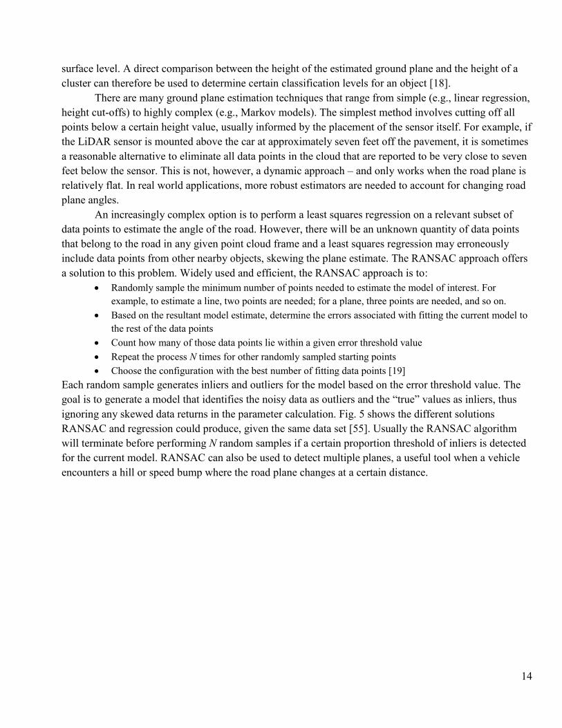
An increasingly complex option is to perform a least squares regression on a relevant subset of

data points to estimate the angle of the road. However, there will be an unknown quantity of data points

that belong to the road in any given point cloud frame and a least squares regression may erroneously

include data points from other nearby objects, skewing the plane estimate. The RANSAC approach offers

a solution to this problem. Widely used and efficient, the RANSAC approach is to:

Randomly sample the minimum number of points needed to estimate the model of interest. For

example, to estimate a line, two points are needed; for a plane, three points are needed, and so on.

Based on the resultant model estimate, determine the errors associated with fitting the current model to

the rest of the data points

Count how many of those data points lie within a given error threshold value

Repeat the process N times for other randomly sampled starting points

Choose the configuration with the best number of fitting data points [19]

Each random sample generates inliers and outliers for the model based on the error threshold value. The

goal is to generate a model that identifies the noisy data as outliers and the “true” values as inliers, thus

ignoring any skewed data returns in the parameter calculation. Fig. 5 shows the different solutions

RANSAC and regression could produce, given the same data set [55]. Usually the RANSAC algorithm

will terminate before performing N random samples if a certain proportion threshold of inliers is detected

for the current model. RANSAC can also be used to detect multiple planes, a useful tool when a vehicle

encounters a hill or speed bump where the road plane changes at a certain distance.

15

Figure 5: Line estimation with RANSAC showing inliers and outliers and possible regression line for the data set [55]

2.2.3 CONVERTING CLUSTERS TO OBJECTS

The identification and removal of the ground plane combined with the down-sampling of the point

cloud into clusters allows the identification of static and dynamic road objects that will support obstacle

detection and identification. While radars inherently sense radial velocity for each data return to aid in this

process, LiDAR systems natively lack this data element. Typically, cluster movement over time is used

instead to provide measurable velocity components of objects within a series of consecutive point clouds.

Based on their position, clusters resulting from earlier processing steps, which are often reported as a

centroid with associated density characteristics, are used to mark areas within the vehicle’s local

occupancy grid as occupied or empty. Once the next successive point cloud frame is available, the process

is repeated to update the vehicle’s surrounding occupancy grid. Over the course of several cloud frames

and occupancy grid formulations, there can only be four progressions: 1) certain areas remain occupied, 2)

remain unoccupied, 3) switch from unoccupied to occupied, or 4) switch from occupied to unoccupied.

Discernible object tracks are then identifiable as additional frames are captured. For a stationary sensor,

those areas that stay occupied can be considered static obstacles. Dynamic obstacles progress to adjacent

occupancy grid locations over time in accordance with a certain path. To aid this, arbitrary object IDs and

age since initial detection are often catalogued within occupancy grid tracks to help identify new objects

as they come into observation (with relatively lower confidence of existence) and continue to follow older

object tracks (observed over time with higher confidence of existence). An object’s last observed age can

also help determine when it is dropped from the tracking list, for example, if it leaves the observable area

and remains untracked for a certain period of time.

2.2.4 OBJECT TRACKING

As previously noted within the discussion pertaining radar, object tracking using time discrete

sensors is an optimal estimation and data association problem where object existence, object state, and

sensor data are all commonly modeled as Gaussian distributions within the state space. Many of the same

16

principles and solutions applicable to radars apply to LiDAR sensor systems as well. Like radar sensors,

LiDAR sensor systems often incorporate KFs to accurately track objects within the sensing environment.

The process and equations are the same, except that these KFs do not initially track velocity components

of clusters as they first become visible. However, with the multi-frame fusion approach previously

outlined, KFs can derive an object’s velocity over time as they move within the structured occupancy grid.

As was the case for radar, data association techniques are required for multi-track functionality

using LiDAR. The algorithms presented in Challa et al. (2011) and Bar-Shalom et al. (2001), such as the

density and probabilistic filters, are also useful here, as well as others based on Euclidean distance and the

global nearest neighbor (NN) procedure. Data association is usually performed after RANSAC processes,

in either the clustering or occupancy grid formulation step. As new data points become available from the

down-sampled point clouds, one option is to assign each formulated return to the NN using Euclidean

distance for single object tracking, or global nearest neighbor (GNN) for multi-object tracking. Here,

GNN uses statistical distance thresholds to assign incoming measurements to a list of N tracks using an

“association cost” matrix. The cost matrix allows the association problem to be transformed into a linear

assignment problem where the minimal cost solution can be solved for using known algorithms, such as

the Hungarian method [20]. Other filters use Euclidean distances or density comparisons to determine

whether data measurements should be associated with current object tracks or new ones created. The

aforementioned JPDA technique or its modifications could also be applied in this context.

2.2.5 OBJECT CLASSIFICATION

Given a myriad of different objects of interest within the driving area, it is useful to classify object

tracks within the point cloud into a few general categories, including vehicle, pedestrian, cyclist, and

environmental objects (e.g., trees, signs, buildings, fences, guardrails). Such object identification allows

the use of more accurate object-specific models to predict its movement. For example, vehicles tend to

stay in the usable road area and continue in their original directions, while cyclists and pedestrians can

turn somewhat unexpectedly. There are a multitude of options employed for LiDAR object classification,

including trained neural networks, support vector machines (SVM) classifiers, and box models. Current

research is often focused on developing quicker and more accurate classifiers.

Each of the five processes described in the previous sections, in the context of a LiDAR-applicable

object tracking system, has been subject to extensive research, particularly since the turn of the century

when laser scanners were seen as promising technologies for ADAS and automated driving

functionalities. For some processes, foundational research was conducted decades before it found use in

LiDAR systems. The original paper outlining RANSAC was published in 1981 by Fischler and Bolles

[19], while an early paper discussing the advantages of the nearest neighbor data association filter that

GNN adapts was published in 1967 by Covert and Hart [20]. And, of course, the optimal tracking paper

that is highly utilized in both LiDAR and radar object tracking was published by Kalman in 1960. Even

the process of point cloud down-sampling is part of the wider field of data clustering. Within that field,

Xu and Tian’s (2015) “A Comprehensive Survey of Clustering Algorithms” is a useful summary of

modern and traditional clustering algorithms [14]. In their discussion, it is obvious that many LiDAR

17

clustering algorithms employed today are adapted from data structures and techniques originally

developed from the graph theory, statistical, and digital electronics fields in the late 1980s and 1990s.

Early research in LiDAR object tracking considered two-dimensional laser scanners. For example,

Mendes et al. (2004) utilized recursive line fitting to identify object clusters within a multi-target detection

scheme [21]. Pattern recognition was then used to differentiate between pedestrians and other obstacles

such as walls; all objects were tracked using a KF. This approach is only applicable to a single laser scan

sensor, far from the three-dimensional LiDAR sensors currently available. As variations of tracking

models continued to be researched for two-dimensional laser scanners, the next progression was to merge

the measurements from multiple such scanners. Mertz et al. (2012) presented that type of sensor fusion

approach applied to four laser scanners placed at varying angles around the vehicle [22]. Multiple laser

scans allowed the system to detect objects at multiple heights, similar to a LiDAR with four channels.

Each individual sensor contributed to a global point scan that is merged into a composite occupancy grid

with associated height maps. Clusters were determined based on the distance between points. Mertz et al.

(2012) also devised a custom ground plane removal scheme that involves calculating the average and

standard deviation of each cell in the height map and then removing returns that are one standard

deviation below the average height. KFs are used for object tracking.

With the implementation of multi-channel LiDARs in the early 2010s, more comprehensive and

computationally efficient algorithms were needed. Azim and Aycard (2012) proposed a tracking

algorithm for a 64-channel Velodyne LiDAR [23]. Here, the point cloud is down sampled into an octree

that feeds into a three-dimensional occupancy grid. Clusters were determined by Euclidian distances in a

region growing fashion – those data points close enough to an adjacent cluster were added to the original

cluster; those that are farther away started a new cluster. Their novel approach involved tracking

occupancy grid cells that change from occupied to unoccupied and vice versa over multiple scans to

hypothesize where dynamic obstacles could be, a process akin to background subtraction from computer

vision. Kalman filters and GNN were used to track and data associate, respectively. This method

represented a major advance in modern filtering techniques but does run into extended computational

times in highly cluttered urban areas. An alternative generative clustering approach was proposed by

Kaestner et al. (2012) [24]. Instead of discriminating between a list of predetermined object classes, their

approach detected a wide range of objects and grouped them together based on spatial proximity. Both

dynamic and static obstacle detection and grouping were achieved for objects as small as a single

pedestrian and as big as a tram without prior knowledge of object parameters. However, at the time this

approach could only process a point cloud every two seconds which makes inapplicable for real time

applications. Zhou et al. (2012), in turn, proposed an alternative object clustering technique they name

“super segments” [25]. The authors first employed RANSAC to identify ground plane points and then

grew clusters from all remaining points. If a point was within a certain distance threshold of an already

determined cluster, it was added to that cluster. However, clusters were limited to a maximum number of

points to ensure adequate sampling. RANSAC was run again on each cluster to obtain cluster plane

normal vectors. All adjacent clusters with similar normal vectors were merged into super-segments. The

authors claimed that these super segments better represent the planar surfaces in the driving area (e.g.,

houses, fences, guardrails) and other individual and smaller objects. General object classifications can be

made based on the characteristics of these super segments. The proposed method is accurate but, at the

18

time, took anywhere between 5-10 seconds to process a frame, limiting its applicability for a real-time

system. A modified approach is presented in Asvadi et al. (2016), who proposed splitting the point cloud

into multiple ground planes using RANSAC, each one further from the vehicle [26]. The remaining points

that lay above these ground planes were considered possible road objects and down sampled into voxels.

The novel aspect was that the incoming point cloud is merged with the five previous frames based on

vehicle odometry measurements, allowing the detection of static and dynamic voxel grid cells. However,

due to the large computational times to merge point clouds, the approach requires between 3 and 4

seconds to process a single frame.

In general, while all of these implementations represent accurate and reliable solutions to LiDAR

point cloud filtering and object tracking, they did not meet real-time system needs given the available

processing power in a typical LiDAR unit. Real-time tracking performance for automotive applications

was not achieved until the second half of the 2010 decade. As computing platform capabilities and data

transfer rates increased, researchers were able to implement and improve filtering algorithms for point

clouds. Most works that achieve real-time capability recognize the need to pre-process point clouds into

more effective data structures, although the overall approach generally remains consistent with earlier

investigations.

One real-time solution is proposed by Wang et al. (2018) through an approach that utilized the

height map of a two-dimensional grid created with a 64-channel LiDAR sensor [18]. Incoming points in

the point cloud were immediately put into an occupancy grid and sorted by height. The authors then sorted

the occupancy grid points to obtain different plane blocks for the whole frame. These planes included data

characteristics such as maximum height, minimum height, and intensity values. Pre-determined height

thresholds were then used to discern plane blocks that are lower and constitute the road layer and plane

blocks that contain objects, whether they be on the road surface or overhanging. In ambiguous cases,

where objects may have a small height value or may be part of a slanted road, the variance in intensity

returns over that plane block can aid its classification as a pavement layer or an object. LiDAR data

intensity return values from pavement, for example, tend to show much smaller variances than those from

pedestrians or other vehicles. From here, Wang et al. (2018) clustered the grid into objects using a

spatially varying threshold. Due to the geometry of the laser planes in the sensor, objects that are further

away in the point cloud have a larger grouping radius threshold value than objects that are closer to the

sensor. The multi-frame fusion approach was used to improve the motion state of tracked objects. An

SVM was used to classify vehicles, pedestrians, and bicycles. The entire process only took 10 ms per

frame, substantially faster than previous solutions. The faster run time is particularly achieved because

Wang et al. (2018) reduced the clustering problem to O(g) time complexity, where g is the number of grid

elements and O is the time complexity of the algorithm, a measure of efficiency

Another real-time solution built around obstacle grids and multi-frame fusion was proposed by Xie

et al (2019) [27]. In their approach, once road segmentation was complete, the point cloud area was

reduced into a 200 x 200 obstacle grid with uniform grid size (~ 40 cm x 40 cm, given the sensor’s FOV).

A novel algorithm, called eight-neighbor cells clustering, clustered groups of adjacent obstacle cells

within the grid. Multi-frame static and dynamic obstacle detection was then carried out by tracking a

subset of points in each obstacle grid over six subsequent frames. A similarity value between each object

based on lateral and longitudinal position was used for data association between frames. Once associated,

19

objects were tracked using a KF and a novel dynamic tracking point box model. Static obstacle detection,

dynamic object tracking, road segmentation, and clustering were performed with an average run time of

96 ms per frame. Xie et al. attained near real-time performance because of their custom clustering

algorithm and the decision to only track moving objects judged to be in the drivable area, thereby

minimizing overhead calculations.

Both aforementioned approaches achieved near real-time processing when tracking objects with a

LiDAR sensor in complicated driving environments. Both implemented fast road segmentation algorithms

and focused on reducing the computational time needed to data associate and track objects. Although both

approaches relied on the reduced resolution of occupancy grids, which can contain thousands of points

themselves, the approaches leveraged the tradeoff between processing the entire point cloud for absolute

accuracy and down-sampled the point cloud for faster computation. Future LiDAR tracking algorithms

will need to make the same tradeoffs, implementing novel versions of occupancy grid formulation based

on different forms of clustering.

Implementation of these approaches into practitioner tools is currently a very dynamic

environment. At this time, pcl offers some implementations of these approaches, including modules for

point cloud transformations between frames for moving sensors; plane estimation and segmentation using

RANSAC; down-sampling point clouds using voxels, octrees, and occupancy grids with height maps;

spatial density estimators for data returns, clustering methods based on Euclidean or statistical distances;

region growing methods; nearest neighbor searches; three-dimensional object detection with centroid

estimators; and GPU-leveraging configurations for computing platforms [13]. The current investigation

leveraged these libraries offered by pcl and the methods in some of these previous investigations to

develop an effective LiDAR tracking solution in a simplified driving environment. Specifically, ground

plane estimation was performed through RANSAC and point cloud filtering was based on generating

voxel grids. From the voxel grids, obstacle clustering with the NN data association technique was

performed. Static and dynamic object classifications was made based on the cluster’s velocity in the

obstacle grid. Finally, a KF implementation was developed to support obstacle tracking. Object

classification was necessary in the controlled environment in which the tests will occur. Any moving

object in the environment was assumed to be a vehicle and modeled as a point object. Given that the

sensors remained static, there was no need for multi-frame fusion or point cloud transformations.

2.3 SENSOR FUSION

Perceptual sensors, such as radar and LiDAR, are rarely used alone to provide perception

information for a vehicle. Generally, these sensors are combined within the same application to provide

redundancy and robustness: the strengths of one sensor can help overcome the weaknesses of another

sensor. For example, LiDARs have great spatial resolution, radars natively provide radial velocity of

tracked objects, cameras provide color information, and ultrasonic sensors can provide distance

measurements at a short range – all of these attributes are useful, if not essential, in attaining a full

environmental scan when trying to traverse roadways. Therefore, common automotive system

architectures often fuse camera and LiDAR, radar and LiDAR, and camera and radar, but any

combination between two or more perception sensors can exist depending on the application and resource

20

limitations. For example, due to their lower costs, some current production vehicles combine camera and

radar to provide Society of Automotive Engineers Level 2 (2018) automated driving features [49].

Leveraging a multitude of sensors to provide accurate and reliable data is critical for automated

driving. Consequently, there is a substantial amount of research that has been conducted pertaining data

filtering and optimization for the implementation of sensor fusion on a diverse range of systems and

sensors. Given the aims of the current investigation, however, the focus of this discussion will remain on

previous work to fuse LiDAR and radar data.

Sensor fusion, in the context of environmental perception, implies combining the data streams or

object outputs of multiple sensors to ultimately reduce the uncertainty about the objects and their current

state. If two sensors perceive the same object in the same global space, the system can be more certain of

its existence and can combine the data from each sensor to better track the object. Sensor fusion

particularly benefits systems that need to perform in complex situations with a variety of potential objects

(e.g., driving a vehicle).

A common goal of sensor fusion in automotive applications is to support object detection and

tracking tasks. There are two primary methods to achieve sensor fusion for this application: decentralized

and centralized fusion. De-centralized fusion focuses on the individual sensors themselves. Each sensor

within the system architecture captures and pre-processes its own data. The tracks from all sensors are

used for input into a fusion module that combines them. Often, a second layer of tracking is applied to

fused tracks to support global object tracking. The process is often referred to as track-to-track fusion

(a.k.a., high level fusion, object list level fusion). Track-to-track fusion offers a straight-forward and

intuitive process to combine sensor readings and outputs that doesn’t require any modifications to sensor-

specific software. Other benefits include low bandwidth requirements and ease of implementation. The

only extra modules needed are those to combine tracks after sensor processing, which often utilize

commonplace data association techniques to manage the global list of object tracks – tracks from two

sensors may converge into one when they track the same object, diverge into two tracks when two close

objects begin to split apart, or be disassociated when one sensor tracks an object not perceived by the

other sensor. Statistical probabilities and model parameters can help determine the occurrence of each

case. Drawbacks of track-to-track fusion generally stem from unsynchronized sensors.

In contrast, centralized fusion uses all sensor data as input before any object detection and

tracking is performed. Incorporating all data from the sensors before running detection and tracking

algorithms ensures that the system has as much data as possible to make decisions. A small amount of

pre-processing is usually done for some sensors (e.g., ground plane removal and general clustering for

LiDARs) leaving only the most important features of each sensor’s measurement frame. These features

conform the input from which a central tracking algorithm can associate and develop tracks. As a result,

centralized fusion is often referred to as low level or feature level fusion. Centralized fusion builds object

identification from the ground up, resulting in a more accurate that is harder to implement than de-

centralized fusion. Large system communication bandwidth is required, as a substantial amount of data

can be available in at any given time, and significant software modifications are generally required for any

unique combination of sensors. The process hinges on initial pre-processing for each sensor to identify

useful data returns. A similar state space then must be established between sensors to support object

mapping, with complexity of this task being dependent on the sensor combination. For example, equating

21

the RGB color frame from camera vision to the x-y-z coordinates of a LiDAR point cloud is very difficult,

but finding congruent state spaces between LiDAR and radar is much easier. Finally, object identification,

tracking, and data association are carried out in the state space based on modified versions of the

previously discussed approaches. Centralized fusion is much easier to implement with sensors that have

similar output structures, such as radar and LiDAR.

Hybrid approaches have also been developed. For example, one sensor may initially identify and

track objects on its own and low-level data from another sensor is combined after that process is complete.

Usually, this allows the system to detect regions of interest (ROI) that the other sensor will augment,

achieving efficiencies in computational time and better tracking within the ROIs. This approach is

particularly useful for systems that use camera vision as a sensor, where tracking is typically done both at

the sensor and fusion levels to produce global tracks.

Much of the earlier sensor fusion work related to automated driving research focuses on systems

that included camera sensors. Kaempchen et al. (2004), for example, used laser scanners to detect possible

objects and regions of interest for a forward-facing camera in order to achieve better adaptive cruise

control features [28]. A hybrid approach is used that employs object tracking at two levels: only with the

laser scanner data, and with camera data added to the laser scanner data. Based on the ROIs identified

from the laser scanner module, the camera uses machine vision techniques to identify a bounding box

around the vehicle ahead of it and performs tracking at the fusion level. Similarly, Aufrere et al. (2003)

focus on camera and laser scanner fusion for short range sensing in urban environments, an area they saw

as particularly important for automated driving functions [29]. Their proposed system implements high

level fusion with feedback loops between the global object list and the sensors own tracking algorithms.

Laser scanners detected objects around the vehicle while the camera tracked the roadside curb. Each

obstacle list is fused into a global map that can be associated with future measurements.

As sensors progressed, laser scanners were replaced by multi-channel LiDARs, although camera

sensors were retained. A low-level fusion approach between these sensors was presented by Mahlisch et

al. (2006) [30]. A forward-mounted LiDAR identified relevant features from the environment and

provides ROIs for the camera to detect vehicles. Distance to the vehicle was estimated directly from the

observed height and the width of the vehicle was estimated from the camera frame. These combined data

measures were provided as inputs to the tracking phase. This method achieved object tracking and

classification with an AdaBoost classifier in about 20 ms per frame under normal highway conditions. A

similar low-level approach was presented by Monteiro et al. (2006) for slow-moving vehicle applications

[31]. A feature extraction module within the laser scanner informed the camera of ROIs in the forward

driving area. The camera performed a search in the identified sub-window, and a coordinate

transformation put the objects identified in the image plane into common coordinates with the LiDAR.

Object tracking and classification were then executed. Wei et al. (2018) described another low-level

fusion method for industrial vehicles [32]. Their approach used a 16-channel LiDAR to detect vertical

“beacons” that mark off-limit zones for the vehicle. The point cloud was first filtered to remove the

ground plane and then all remaining clusters were run through an SVM for beacon identification. At the

same time, a camera module used neural networks to identify and calculate beacon locations within the

camera frames. The detections were finally fed into a fusion model where object tracking and final

confidence values calculated. The system runs at 5 Hz, which was considered acceptable for slow-moving

22

vehicle needs. In all three of these examples, LiDAR is a useful tool for low-level feature extraction that

can inform other sensors of specific regions of interest with high spatial accuracy.

Radar has also been paired with cameras to provide greater positional accuracy. Andersson (2017),

for example, developed a high-level fusion method between radar and camera sensors [33]. The non-real-

time approach centered on a module for radar Kalman filtering and pre-calculated positions of objects

from the camera. The combination of the two tracks in the fusion module made use of data association

and model predictive techniques to perform better than standard tracking software. Ekstrom and Risberg

(2018) presented a similar high-level fusion approach, but with simulated stereo vision tracks [34]. The

approach used a vehicle box model and an EKF to track forward vehicles with radar. These tracks were

then combined with the simulated stereo vision tracks in the fusion model in two ways: combining the

tracks to produce global object paths, and feeding these global object detections back into the radar for

better data association. Both of these approaches demonstrated increases in tracking accuracy with sensor

fusion although they relied on simulated data and non-real-time calculations.

A substantial body of research has examined fusion between the two sensor of interest in this

investigation, radar and LiDAR. An early high-level fusion approach between these sensors was presented

by Blanc et al. (2004) for vehicle detection on the forward roadway [35]. The process tracked vehicles

with the radar, using a KF, and the LiDAR, matching data clusters with a vehicle model. The output tracks

were then supplied to a fusion module that combined the tracks and added another layer of Kalman

filtering to improve accuracy. The addition of LiDAR assisted in differentiating the lane positions of

vehicles at greater distances and providing more accurate velocities than only using radar. Radar and

LiDAR sensors, however, have immensely progressed over the last decade in the amount and resolution

of data they generate, and modern fusion algorithms have to account for this.

In that vein, Gohring et al. (2011) presented a hybrid low-level fusion algorithm between a front

facing radar and an Ibeo LiDAR in a highway vehicle following scenario [36]. The fusion module offered

better tracking of the front vehicle than attained with a single sensor and provided a maintained global

object list for the vehicle dynamics controller. The radars used directly reported an object list – raw data

returns for each cycle were not available. Distance-based clustering was performed with the LiDAR point

cloud to extract features, with object detection left to the fusion module. As asynchronous sensor data was

obtained, the fusion module attempted to data associate it with an already identified track using the NN

technique. KFs were used at the fusion level to track objects and confidence levels, which were passed to

the sensor layer to help with feature extraction. The fusion technique leveraged the advantages of both

sensors during the on-road tests: velocity positions were slightly better than using only the radar, and

positional estimates were better than using only the LiDAR.

A fully implemented high-level fusion method like Gohring et al.’s was proposed by Hajri and

Rahal (2018) for forward vehicle tracking on highways and highly curved roads [37]. Focus is on the

fusion side of the problem, with object list outputs of the sensors used as direct inputs to the fusion model.

As asynchronous data was obtained from the sensors, the fusion model considered the movement of the

vehicle since the last recorded measurement and attempted to data associate each object to previously

defined obstacle tracks using the GNN method. The fusion model maintained tracks with a constant

velocity KF and determined when certain sensor measurements required the addition of a new object track

and when an object could no longer be tracked. Building off Gohring et al.’s testing methods, forward

23

vehicle position and velocity estimates were conducted using just the radar, just the LiDAR, and with the

fusion method. More robust tracking was achieved with the fusion method.

In contrast, Na et al. (2014) offered a more general-purpose hybrid fusion approach between radar

and LiDAR [38]. Radar reported objects automatically, but the point cloud coming from the Ibeo LiDAR

was processed by the researchers. First, the point cloud was condensed from three to two dimensions

regardless of return height. Then, based on the density of the returns in neighboring cells within the two-

dimensional space, different objects were partitioned. The fusion module took as inputs the object list

from the radar and the object list from the LiDAR and performed KF tracking. Probabilistic data filters

assigned object measurements to tracks. Un-associated measurements were placed in new tracks and a

track manager deleted tracks if they were not associated with an incoming measurement over a certain

number of frames. Multiple tracks could claim a single incoming measurement based on its probabilistic

weight. Due to the large amount of down-sampling in the point cloud, the approach could process a single

urban-environment frame in under 10 ms.

Cho et al. (2014) extended these fusion methods from forward vehicle detection to detection of

objects at any position around the vehicle [39]. The research-level sensor suite paired six radars with six

four-channel LiDARs to provide a 360° FOV. The feature-level fusion approach tasked the sensors to

preprocess raw data and extract useful features: radars reported cluster points and LiDARs removed the

ground plane, clustered the point cloud, and identified vehicles based on “L” shaped corners. Features

from this process were asynchronously fed into the fusion module which data associated each feature to a

track using the NN approach and sensor-specific modeling parameters. Objects further away were

modeled as a point; closer objects were modeled with a three-dimensional bounding box to estimate

volume. An EKF was used for the prediction and update steps of the object tracker. Rear- and forward-

facing cameras were included to aid object classification (e.g., vehicle, pedestrian, cyclist) and

consequently in determining the best dynamic model for each object. Results showed computational times

of 100-200 ms for the multi-sensor fusion; somewhat slower than the needs of current real time systems.

Table 2 provides a brief summary for those works mentioned above. Table 2: Sensor fusion past work summary

RADAR LIDAR/LASER

SCANNER

CAMERA YEAR DISTINGUISHING

FEATURES

KAEMPCHEN

ET AL. X X 2004

Hybrid approach with ROI

identification with laser scanner and

then bounding box defined with

camera.

AUFRERE ET

AL X X 2003

High level fusion with camera tracking

the roadside curb and a laser scanner

detecting close objects.

MAHLISCH ET

AL. X X 2006

Low-level fusion with ROIs identified

with LiDAR and then camera vision

estimates vehicle size.

MONTEIRO ET

AL. X X 2006

Low-level fusion with ROIs identified

by the LiDAR and then combined with

camera vision data at low speeds.

Classification performed after this.

WEI ET AL. X X 2018 Low-level fusion at low speeds that

identifies beacons with the LiDAR and

24

then combined with object tracking

from camera vision.

ANDERSSON X X 2017 High-level, offline fusion technique

that combined radar KF tracks with

camera vison object positions.

EKSTROM AND

RISBERG X X 2018

High-level fusion approach between

radar objects and simulated stereo

vision objects with track information

feedback option for the radar.

BLANC ET AL. X X 2004

High-level fusion approach with radar

tracks and simplified LiDAR detection.

Obtained better lane position estimates

at larger distances.

GOHRING ET

AL. X X 2011

Hybrid approach that combined radar

objects and LiDAR clusters. Fusion

module performed object classification.

HAJRI AND

RAHAL X X 2018

High-level fusion that combines the

tracks of the radar and LiDAR to track

forward objects more accurately than

just using a single sensor.

NA ET AL. X X 2014 Hybrid approach that combines radar

tracks and LiDAR clusters in urban

driving scenarios.

CHO ET AL. X X 2014

Low-level approach that uses radar

clusters and feature extraction from the

LiDAR to provide object tracking in a

360° FOV.

Regardless of the fusion approach, these previous efforts indicate the need for extensive filtering

of the LiDAR point cloud to extract features of interest and to, when feasible, directly use the radar’s

object list. Objects are generally associated with previous tracks using a KF and common association

techniques. Use of the global object list to inform low-level sensor filtering seems to be useful.

Essentially, however, all fusion methods for radar and LiDAR are built at some level off the basic, single

sensor tracking methods presented earlier, with choices made in terms of the stage(s) at which object

tracking occurs and which KF version is applied (and at which stage(s)). In this investigation, a track-to-

track fusion technique was used. Sensor object tracks were conducted at radar and LiDAR sensor level as

an intermediate step, with a central track fuser combining sensor tracks as a final step. The high positional

accuracy of the LiDAR helped to improve track accuracy when combined with those of the radar.

2.4 SCALED TEST BEDS

For a full-sized vehicle, the methods presented in the previous two sections offer enough

background to initiate advanced development of a fusion system in support of autonomous driving

systems. However, the current investigation intends to implement a fusion solution for a small-scaled

vehicle in a small-scaled environment. This scaled testbed (STB) vehicle and its scaled environment

present novel challenges for fusion methods, especially those involving radars.

STBs collectively refer to any small-scaled vehicle that resembles the sensor suite and the

functionality of full-sized vehicles. STBs allow for initial testing of certain vehicle systems on the small-

scale vehicle with subsequent deployment on their full-size counterpart. Test usefulness is a direct

25

function of the resemblance between the STB and its full-sized counterpart. Fully-featured STBs allow

testing of vehicle control inputs, dynamic characteristics during the driving tasks, and as of late, ADAS

functions with specific sensors and data filtering algorithms.

Equipping STBs with the same sensors and controls as full-sized vehicles is the first step to

achieve vehicle similitude. Most small-scaled vehicles adapt Remote Control car platforms at either the

1/4th, 1/5th, or 1/10th of the actual size because powertrain components at that scale are readily available.

Required sensors and computer hardware are then added to the existing platform. STBs generally feature

inertial measurement units, accelerometers, gyroscopes, a central electric motor with differential or

individual motors for each wheel, wheel speed sensors, steering servo motors, on-board central processing

units (CPUs) for motor and steering control, and ethernet or wifi connection ports. Some sophisticated

STBs may also feature additional ADAS sensors such as laser scanners, LiDAR, stereo vision hardware,

cameras, ultrasound sensors, GPS modules, and the additional microcontrollers and connection ports

required to deploy these sensors. Capable on-board CPUs along with careful system design is required,

particularly as additional sensors are introduced.

In general, STBs offer several advantages for engineers and developers. First, expense – STBs are

less expensive to create than a full-sized prototype vehicle. Second, time – STBs require less time to

build; tests using STBs are easier and faster to conduct than those on full-sized vehicles. Third, risk –

STBs reduce the physical risk for all people involved in the testing which ultimately reduces business risk.

Fourth, reality – STBs can more easily expose a vehicle’s physical limitations and more intuitively

demonstrate vehicle functionality than software simulations. Overall, STBs are one tool in a large

toolchain available for systems development engineers and efficiently bridge virtual testing and full-scale

implementation. When used in combination with other approaches, STBs can accelerate the development

of driving functions, especially when used for physical “smoke” tests of certain ADAS aspects.

The use of STBs for automotive research is not novel. Early models aimed at ADAS function

testing began to be developed in the late 1990s. As automated driving progressed, STBs adapted to

incorporate many of the required sensors. Early on, STBs were used to test vehicle dynamics and software

controllers. One of the first modern systems was proposed by Brennan and Alleyne (2001) [40]. This STB

used a 1/5 scale vehicle with various configurations, including two-wheel and four-wheel drive with direct

current motors and two- and four-wheel steering. The STB vehicle ran on a moving beltway and was

hardwired to a computer via ethernet. Extensive dynamic similitude testing and control designs for speed

and steering motors were conducted with the STB, with results extrapolated to a full-sized vehicle.

Longoria et al. (2004) presented another STB vehicle implementation used to test anti-lock braking

dynamics [41]. The 1/5 scale STB vehicle was outfitted with front disk brakes, drive shaft encoders, and

control units to measure braking profiles when ABS was activated after a hill descent. Dynamics between

the STB vehicle and a full-sized vehicle were compared. Electronic stability control tests were performed

with an STB by Katzourakis and Katzourakis (2008) [42]. Using gyroscopes, accelerometers,

potentiometers, wheel encoders, and other microcontrollers, the research focused on control inputs for

vehicle dynamics for different turning radii.

As automated driving has progressed, STBs have followed suit to allow testing of the wide range

of sensor applications needed for advanced driving systems. Xu et al. (2017) developed the PaTAVTT

STB [43]. The STB vehicles for Xu et al. (2017) incorporated the basic motors and sensors needed for

26

dynamic control but augmented with cameras, ultrasound sensors, and an indoor positioning system.

Cameras are used to detect lane lines, ultrasound sensors detect forward objects, and the positioning

system measures vehicle dynamics and trajectory following. Specific tests were conducted to assess traffic

flow questions and U-turn dynamics. More recently, an open source and highly adaptive 1/10th scale STB

is presented by O’Kelly et al. (2019) [44]. F1/10, as the STB was coined, utilizes IMUs, LiDAR, video

camera, on-board computing, and ROS packages to test a multitude of automated driving functions, such

as simultaneous localization and mapping (SLAM), forward collision warning, trajectory planning and

following, camera vision applications, lane keeping, and vehicle-to-vehicle communications. The STB

included a system for a driver to teleoperate the vehicle with a steering wheel and pedals. Many of the

algorithms tested at small scale were implemented later in a full-sized vehicle.

Some commercial outfits have offered highly capable and adaptable STBs aimed at removing the

start-up barriers for automated driving research, especially research focused AI applications. Qcar,

Quansar’s self-driving research STB, commercially available, is a 1/10th scale vehicle that mimics the

automated driving systems of current automated vehicles. The vehicle includes open source code pre-

installed and accommodates other open source plugins like TensorFlow. Navigation algorithms, mapping,

V2V communication, object detection, camera vision, and other common ADAS functions run off the

sensory and compute systems platform, which includes on-board computing, dynamic controls, a laser

scanner, four cameras, stereo-vision, and wifi connectivity [45]. Similarly, Clear Path Robotics Inc. offers

the Jackal Unmanned Ground Vehicle. An entry-level robotics research platform, the Jackal is a small but

rugged four-wheel vehicle with plug-ins for different robotics or automated driving needs. Equipped with

a powerful on-board CPU and other advanced sensors such as differential GPS, cameras, and stereo

vision, the Jackal can serve as a tool for quick and precise research for autonomous navigation.

Applications such as machine vision, AI, and path following are supported [46]. Both the Jackal and Qcar

can aid researchers in quickly developing automated driving functions at small scale with many industry-

standard sensors and computing platforms. The platforms feature easily expandable input/output

interfaces and plugins for software tools such as MATLAB, Simulink, python, and TensorFlow.

Despite the impressive configurations of the Jackal, Qcar, and those that came before them, no

STB was discovered that incorporated automotive grade radar into its functionality, as is required by the

current investigation. Because interpreting radar data at small scale is not currently a straightforward

process, radar is either completely left out or an ultrasound sensor is used in its place. Consequently,

although these STBs are highly adept at modeling the ADAS of some full-sized vehicles, any systems that

require radar cannot be directly tested without workarounds or simulated data. Thus, all currently-

available STBs lag in useful functionality when it comes to radar. This represents a sizeable problem

because many ADASs and other highly-automated driving systems rely heavily on radar object detection.

Without including radar, STBs cannot be fully utilized by engineers and developers of automated driving

algorithms.

The solution proposed in the current investigation directly addressed this gap in functionality for

STBs. The fusion method between LiDAR and radar used the high spatial resolution of the former sensor

to inform the latter sensor about potential object locations that the radar cannot reliably detect at small

scale. This fusion process, thus, allowed an STB to fully implement a production radar for general

purpose vehicle tracking within a scaled environment.

27

2.5 CONCLUSION

There are certain key processes in object detection and tracking for autonomous driving systems

that employ radar and LiDAR – two sensors found in many ADAS and automated vehicle

implementations. The processes include Kalman filtering and EKFs, point cloud clustering, ground plane

detection, and data association. Depending on the application, sensor fusion approaches may also be

necessary. Indeed, these fusion approaches are essential when working directly with STBs, which are the

principal tool to be leveraged in this investigation. The resources described in this review are not all-

encompassing. Instead, the intention in each summary was to portray key work and associated general

research trends.

The STB implemented in this investigation will operate in a simplified environment with minimal

clutter in order to focus on the underlying functionality of the system. No advanced tools such as neural

networks, machine vision, or adaptable object classifiers was required, and data clustering was used to

resolve raw data into a small number of objects of interest. In doing so, the techniques presented in this

literature review proved useful in developing the required filtering and tracking algorithm frameworks.

The fusion module in this investigation was in turn built off the implementations and resources previously

mentioned to develop a simple but effective real-time object detection and tracking system that allowed

STBs to use automotive grade radars in combination with LiDAR to track a vehicle in a scaled

environment.

2.6 RESEARCH QUESTIONS

The gaps identified via the literature review suggest a number of important research areas related

to the effectiveness of radar sensors in scaled environments and the ability of other sensors (e.g., LiDAR)

to supplement any shortcomings in radar performance. Based on these gaps, this investigation intends to

answer the following questions regarding scaled vehicle tracking and sensor fusion:

1. Compared to full-scale radar tracking, how much does the positional accuracy of a Radar Tracking

System (RTS) diminish when tracking objects in a 1/5th scaled environment?

2. Can the RTS tracking accuracy in a 1/5th scaled environment be quantified using standard error

metrics?

3. Using a LiDAR sensor and a custom track-to-track sensor fusion technique, can the tracking

accuracy in a 1/5th scaled environment be improved?

a. If present, can the accuracy improvement in the 1/5th scaled environment match the

accuracy obtained from the radar at full scale?

4. Can the custom fusion software and LiDAR clustering algorithms operate in real time using

current consumer-grade hardware?

28

CHAPTER 3 – METHODS

To answer the questions outlined in Chapter 2.6, five elements needed to be implemented. The

first was the radar and associated tracking software; the second, LiDAR clustering of point cloud data; the

third, a software fusion technique; the fourth, a ground truth measurement; and the fifth, a data recording

system with sensor implementation for vehicle trial runs. In this work, radar and LiDAR object tracks

were independently formulated with data from each sensor and an implemented EKF with the JPDA

technique. A central tracker was then developed and used to fuse and combine tracks from each of the

sensors. Finally, location and size accuracy metrics were calculated and compared between differential

GPS (DGPS) ground truth values and the RTS performance on a full-scaled vehicle, the RTS performance

on the 1/5th scaled vehicle, and the fusion technique performance on the 1/5th scaled vehicle. The

following sections provide additional detail for each of these elements of the overall process.

3.1 SENSOR IMPLEMENTATIONS AND TRIAL RUNS

The first step in developing tracking filters was to implement a data collection system in ROS to

capture radar data returns, LiDAR point clouds, and DGPS ground truth values for each vehicle under

surveillance (VUS).

ROS can inherently record and time stamp all messages passed within the system, so the only

input information required were the sensor configurations. Using a developed ROS driver for the

Continental ARS430 series radar running at 14 Hz, the provided Velodyne ROS driver for the Velodyne

PUCK LiDAR set to run at 10 Hz, and custom DGPS ROS drivers, an NVIDIA Nano CPU running Linux

was tasked with collecting data for the trial runs. The radar and LiDAR were statically mounted 10 and

20cm, respectively, off the ground, similar to their height when mounted on a small-scale vehicle. Fig. 6

shows sensor FOVs for both radar and LiDAR.

Figure 6: Sensor FOV configurations

29

Each trial run included a single VUS running through vehicle maneuvers within the radar and

LiDAR’s FOV in a cluttered, but mostly static environment. Curbs, light posts, fences, and other

stationary vehicles were present, but the VUS was the only moving object within the FOV. There were

three main types of vehicle maneuvers: driving directly toward or away from the radar sensor, driving

diagonally across the radar’s FOV, and performing S-turns within the radar’s FOV (Fig 7). The first two

sets of vehicle maneuvers represented normal driving conditions that the perception sensors and their

trackers should easily be able to handle, while the third type of vehicle maneuvers, the S-turns, should

challenge the trackers because of the large non-linear movement. The “S-turns” trials were intended to

represent driving conditions that would be less apparent within the FOV of the radar or LiDAR sensors

than the “Diagonal” and “Straight” trials, particularly if these sensors were installed on a vehicle driving

in real world conditions. More extreme vehicle maneuvers, like “figure 8’s” or circles, were not

considered because these maneuvers would rarely be present in real world driving conditions.

All maneuvers were repeated for the small-scale and full-scale vehicles. The full-sized vehicle

traveled at speeds between 10-15 mph (4.5 – 6.7 m/s) while the small-scaled vehicle traveled at speeds

between 2-4.5 mph (0.89 – 2 m/s). Speeds were limited in each case by the vehicle scaling. A low speed

shuttle is modeled by the small scaled vehicle at 1/5th the size, and, therefore, traveled at 1/5th the speed.

Typical low speed shuttles operate at 10 mph or slightly faster, so the full-sized vehicle attempted to

maintain similar speeds while the small scaled vehicle was driven at approximately 1/5th those speeds for

comparison. Popularity in low speed shuttles with advanced driving systems has increased in the past

decade, with many automotive manufacturers and suppliers, such as Continental Automotive, becoming

interested in developing advanced driving solutions for these vehicles [60]. Thus, the small scale vehicle

used in this investigation was modeled from a low speed shuttle (Fig. 8). The small scale vehicle’s wheel

base was approximately 1/5th that of a full scale low speed shuttle and, like the full scale vehicle, included

both front and rear steering capability. The small scale vehicle featured a top shelf that was located on top

of the motor and steering servos and provided a platform for other sensors, such as the DGPS board (not

pictured in Fig. 8). The vehicle was driven manually using a remote control device during all the trials.

To accurately scale the small vehicle maneuvers, particularly during the “S-turns” trials, tape was

placed at roadway locations where the vehicle should start to change its direction from left-to-right or

right-to-left. However, exact positional scaling was not possible due to the use of a manual driving

approach – thus, the small scale “S-turn” trials extend to positions slightly outside than the full scale “S-

turns” trial when accounting for scale.

All tests were completed during the day with partly cloudy weather conditions and no rain or water

on the ground. No effects of sunlight or other environmental conditions were seen in the collected data

from any sensor. Each run typically lasted for 20 – 30 seconds. Tests of this duration usually generated

280 – 430 radar frames and 200 – 300 LiDAR point clouds.

30

Figure 7: Possible vehicle maneuvers

Figure 8: 1/5th scaled vehicle

ArduSimple DGPS boards provided ground truth values for each trial run. One of the boards,

configured as a DGPS base station through a multi-hour survey, sends GPS timing corrections to the other

board, configured as a rover and installed on the VUS. The ArduSimple system was able to calculate

highly accurate position system with error measurements no larger than 12cm any given time, based on

recorded pilot data being compared to known positions. Latitude and longitude coordinates were

transformed to local sensor coordinates by the DGPS ROS parser.

For each trial run, ROS recordings for all the sensors were timestamped and stored in .bag files for

easy playback.

31

3.2 RADAR TRACKING SOFTWARE

Radar tracking software was developed and implemented in the MATLAB environment as part of

this investigation. The RTS centered on the Extended Kalman filter (EKF) and the principles previously

summarized as part of the literature review. In general, the RTS needed to obtain the radar data returns,

filter those returns based on the sensor speed to identify moving objects, cluster returns from the same

object, perform object tracking, and save the resultant track information for the duration of each trial. A

JPDA point tracker was selected for tracking maneuvering objects within MATLAB as pilot testing

suggested that it was the most consistent and tunable tracker out of the alternatives considered1. The

JPDA displayed the least amount of track switches, lowest false positives in track confirmations, and best

ability to ignore clutter during trial runs.

Raw radar measurements were recorded in the radar sensor coordinate frame. Range (𝜌), angle

(ϴ), and range-rate (�̇�, along a radial axis from the radar sensor itself) values (Eqn. 11) with timestamped

data and other information like radar cross-section (RCS), probability of false detection, signal to noise

ratio (SNR), and variance values were recorded for each raw radar data point. There were typically around

100 radar returns per cycle for the JPDA tracker to use. Measurement noise standard deviation values

were assumed for each measurement state: 1 m for range values, 1° for angle values, and 0.5 m/s for

range-rate values. The corresponding variance values were then calculated as the square of the standard

deviations and passed on to the tracker as the measurement variance (Eqn 12). These standard deviation

values were adapted from the technical specifications for the radar and generalized for the entire viewing

area. Although the expected radar accuracy was higher in some situations, the assumed values produced

higher accuracies over the entire FOV when incorporated into the trackers’ logic as a measurement

variance matrix.

With measurements recorded and being passed to the tracker, the next step was to filter points

based on speed. Because the radar is statically mounted and the tracker is only interested in moving

objects, any measurement that had a range-rate value of 0, or very close to 0, most likely originated from a

static object in the environment and was discarded. Usually, when a radar is mounted to a moving vehicle,

all data returns from a cycle need to be transformed into the vehicle frame with velocity components in

the x and y directions (where they can then be similarly filtered based on ego vehicle speed). Here, that

step is not needed and range-rate values were directly used with a RANSAC algorithm to identify

dynamic radar returns.

The next processing step involved the JPDA. As a point tracker, the JPDA could not take in

multiple data returns and assign them to one vehicle track. Therefore, an algorithm was needed to cluster

measurements that were thought to come from a single object. Two clustering approaches were

considered, one that uses the relative distance between points and one that considers the spatial density of

certain returns. Ultimately, density-based clustering was chosen for this work because of its accuracy in

pilot tests and its ability to differentiate objects in close proximity based on range rate values. To achieve

clustering, measurements required a certain number of adjacent points within a given search radius to be

1 Other trackers investigated for this work included global nearest neighbor (GNN) point trackers and extended object trackers

such as the Gaussian mixture probability density filter with rectangular vehicle models. While extended object trackers offered

vehicle size estimations, they were most susceptible to noisy data (which generally characterizes radar recordings).

32

assigned to the same cluster; the search was then free to move on to any of the points identified within the

search radius. If they had the minimum number of points within their own search radius then they, too,

were assigned to the cluster – if they did not, they were labeled as extraneous. The algorithm works

through each point not assigned to a cluster until all were assigned to one of the clusters or labeled as

noise. It is important to note that the density based clustering considered each dimension of the

measurement, including the range-rate value. If a point was not within the correct range-rate value for a

particular cluster, it would not be assigned to that cluster. In general, this helps differentiate objects that

are traveling at different speeds within close proximity. The final step to clustering was to calculate the

centroid of each cluster and the appropriate measurement noise for that centroid. Averages for each

dimension were calculated from the points included in each cluster and used as the centroid for the cluster.

The new measurement noise was found as the average noise of all the returns (consistent for all

measurements in the case), plus the differences between the average value and measurement values in

each dimension scaled by how many points were in the cluster [56]. Clusters with a larger number of

points (i.e., a large number of points in space that maintain a minimum density) had a smaller

measurement covariance than clusters with a fewer number of points. In essence, because constant values

were assigned to measurement noise for the individual returns, the more points there were for a cluster,

the more confidence that this cluster truly existed, which would be reflected by lower covariance values.

However, thresholds were set for the clustering algorithm such that, if any points were clustered and

assigned to a cluster, there was high confidence that the radar sensed something that was actually there.

The resulting centroids were then passed on to the JPDA to start tracking.

The JPDA filter reported object tracks with an EKF in the tracking frame – x and y dimensions

with velocity components (Eqn. 13) and the radar sensor at the origin facing along the x-axis. The EKF,

itself, had a number of important attributes that needed to be defined before any tracking started: the

process noise, the state transition model, and the mapping (measurement) function.

Process Noise

Process noise standard deviation values of 1 m in both the x and y directions modeled any error in the

dynamic model for the VUS. A value of 1m allowed the filter to incorporate some expected non-linear

motion. With tracking point filters, when the VUS is maneuvering, the cluster centroid may shift

depending on the orientation of the vehicle, or just slightly from cycle to cycle. The process noise values

selected helped the filter model these slight changes in a shifting tracking point. In general, the process

noise was modeled as non-additive noise, meaning the variance associated with each prediction forward in

time for the EKF was independent from the previous timestamp prediction.

State Transition Model

The state transition model, F, was determined by the constant velocity motion model chosen. This

predicted our state vector forward to a specific time (dT) based on previous positioning and velocity

readings (Eqn. 14). The constant velocity motion model ensured only the position estimates of the states

changed while the velocity components stayed the same. Adequate noise components scaled by the time

step were added to the state after propagation and based off the Jacobian of the motion model. Referred to

as time-discrete white noise, W, both the current and the previously assigned process noise were directly

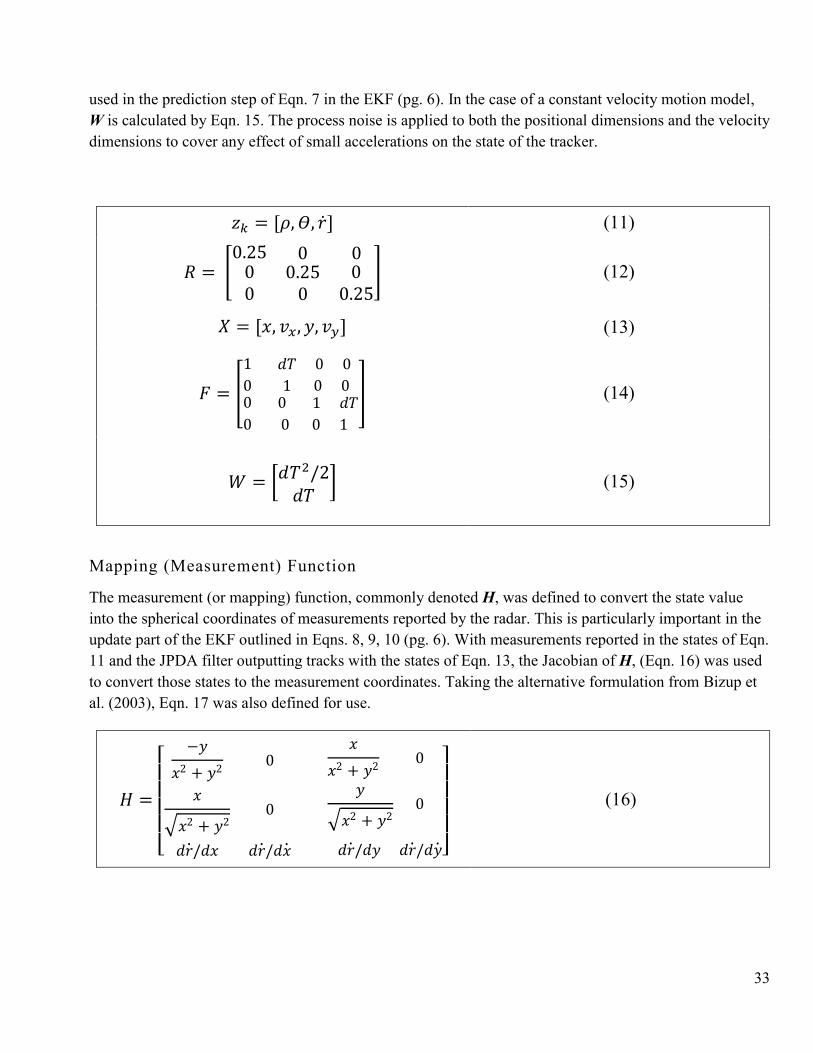
33

used in the prediction step of Eqn. 7 in the EKF (pg. 6). In the case of a constant velocity motion model,

W is calculated by Eqn. 15. The process noise is applied to both the positional dimensions and the velocity

dimensions to cover any effect of small accelerations on the state of the tracker.

𝑧𝑘 = [𝜌, 𝛳, �̇�] (11)

𝑅 = [0.25 0 000

0.250

00.25

] (12)

𝑋 = [𝑥, 𝑣𝑥, 𝑦, 𝑣𝑦] (13)

𝐹 = [

1

0

𝑑𝑇 0 0

1 0 00

0

0 1 𝑑𝑇

0 0 1

] (14)

𝑊 = [𝑑𝑇2/2

𝑑𝑇] (15)

Mapping (Measurement) Function

The measurement (or mapping) function, commonly denoted H, was defined to convert the state value

into the spherical coordinates of measurements reported by the radar. This is particularly important in the

update part of the EKF outlined in Eqns. 8, 9, 10 (pg. 6). With measurements reported in the states of Eqn.

11 and the JPDA filter outputting tracks with the states of Eqn. 13, the Jacobian of H, (Eqn. 16) was used

to convert those states to the measurement coordinates. Taking the alternative formulation from Bizup et

al. (2003), Eqn. 17 was also defined for use.

𝐻 =

[

−𝑦

𝑥2 + 𝑦20

𝑥

𝑥2 + 𝑦2 0

𝑥

√𝑥2 + 𝑦20

𝑦

√𝑥2 + 𝑦2 0

𝑑�̇�/𝑑𝑥 𝑑�̇�/𝑑�̇� 𝑑�̇�/𝑑𝑦 𝑑�̇�/𝑑�̇�]

(16)

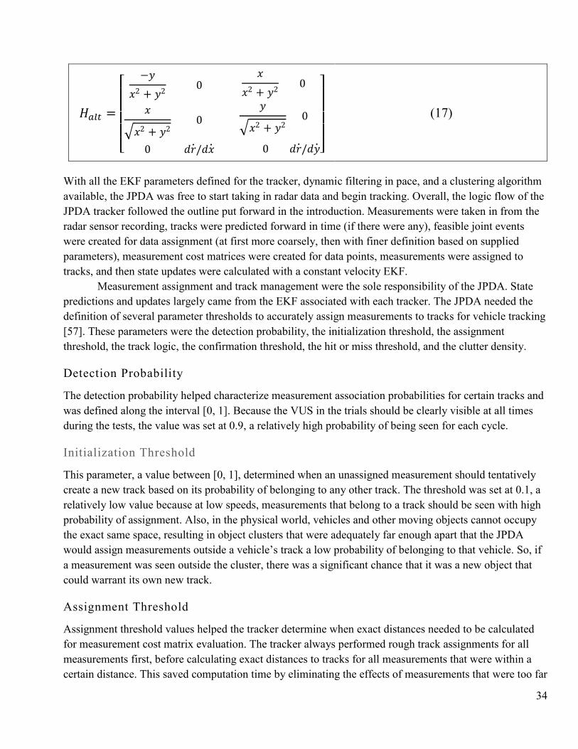
34

𝐻𝑎𝑙𝑡 =

[

−𝑦

𝑥2 + 𝑦20

𝑥

𝑥2 + 𝑦2 0

𝑥

√𝑥2 + 𝑦20

𝑦

√𝑥2 + 𝑦2 0

0 𝑑�̇�/𝑑�̇� 0 𝑑�̇�/𝑑�̇�]

(17)

With all the EKF parameters defined for the tracker, dynamic filtering in pace, and a clustering algorithm

available, the JPDA was free to start taking in radar data and begin tracking. Overall, the logic flow of the

JPDA tracker followed the outline put forward in the introduction. Measurements were taken in from the

radar sensor recording, tracks were predicted forward in time (if there were any), feasible joint events

were created for data assignment (at first more coarsely, then with finer definition based on supplied

parameters), measurement cost matrices were created for data points, measurements were assigned to

tracks, and then state updates were calculated with a constant velocity EKF.

Measurement assignment and track management were the sole responsibility of the JPDA. State

predictions and updates largely came from the EKF associated with each tracker. The JPDA needed the

definition of several parameter thresholds to accurately assign measurements to tracks for vehicle tracking

[57]. These parameters were the detection probability, the initialization threshold, the assignment

threshold, the track logic, the confirmation threshold, the hit or miss threshold, and the clutter density.

Detection Probability

The detection probability helped characterize measurement association probabilities for certain tracks and

was defined along the interval [0, 1]. Because the VUS in the trials should be clearly visible at all times

during the tests, the value was set at 0.9, a relatively high probability of being seen for each cycle.

Initialization Threshold

This parameter, a value between [0, 1], determined when an unassigned measurement should tentatively

create a new track based on its probability of belonging to any other track. The threshold was set at 0.1, a

relatively low value because at low speeds, measurements that belong to a track should be seen with high

probability of assignment. Also, in the physical world, vehicles and other moving objects cannot occupy

the exact same space, resulting in object clusters that were adequately far enough apart that the JPDA

would assign measurements outside a vehicle’s track a low probability of belonging to that vehicle. So, if

a measurement was seen outside the cluster, there was a significant chance that it was a new object that

could warrant its own new track.

Assignment Threshold

Assignment threshold values helped the tracker determine when exact distances needed to be calculated

for measurement cost matrix evaluation. The tracker always performed rough track assignments for all

measurements first, before calculating exact distances to tracks for all measurements that were within a

certain distance. This saved computation time by eliminating the effects of measurements that were too far

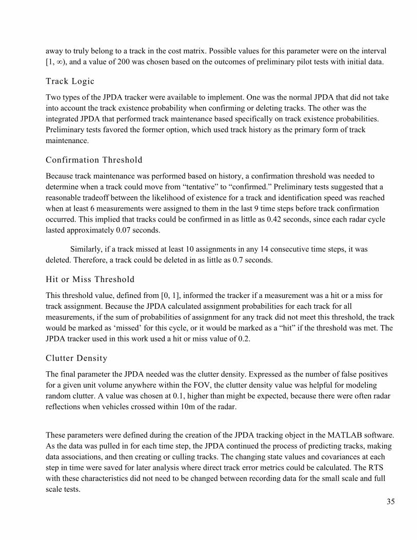
35

away to truly belong to a track in the cost matrix. Possible values for this parameter were on the interval

[1, ∞), and a value of 200 was chosen based on the outcomes of preliminary pilot tests with initial data.

Track Logic

Two types of the JPDA tracker were available to implement. One was the normal JPDA that did not take

into account the track existence probability when confirming or deleting tracks. The other was the

integrated JPDA that performed track maintenance based specifically on track existence probabilities.

Preliminary tests favored the former option, which used track history as the primary form of track

maintenance.

Confirmation Threshold

Because track maintenance was performed based on history, a confirmation threshold was needed to

determine when a track could move from “tentative” to “confirmed.” Preliminary tests suggested that a

reasonable tradeoff between the likelihood of existence for a track and identification speed was reached

when at least 6 measurements were assigned to them in the last 9 time steps before track confirmation

occurred. This implied that tracks could be confirmed in as little as 0.42 seconds, since each radar cycle

lasted approximately 0.07 seconds.

Similarly, if a track missed at least 10 assignments in any 14 consecutive time steps, it was

deleted. Therefore, a track could be deleted in as little as 0.7 seconds.

Hit or Miss Threshold

This threshold value, defined from [0, 1], informed the tracker if a measurement was a hit or a miss for

track assignment. Because the JPDA calculated assignment probabilities for each track for all

measurements, if the sum of probabilities of assignment for any track did not meet this threshold, the track

would be marked as ‘missed’ for this cycle, or it would be marked as a “hit” if the threshold was met. The

JPDA tracker used in this work used a hit or miss value of 0.2.

Clutter Density

The final parameter the JPDA needed was the clutter density. Expressed as the number of false positives

for a given unit volume anywhere within the FOV, the clutter density value was helpful for modeling

random clutter. A value was chosen at 0.1, higher than might be expected, because there were often radar

reflections when vehicles crossed within 10m of the radar.

These parameters were defined during the creation of the JPDA tracking object in the MATLAB software.

As the data was pulled in for each time step, the JPDA continued the process of predicting tracks, making

data associations, and then creating or culling tracks. The changing state values and covariances at each

step in time were saved for later analysis where direct track error metrics could be calculated. The RTS

with these characteristics did not need to be changed between recording data for the small scale and full

scale tests.

36

3.3 LIDAR CLUSTERING

Like tracking for radar measurements, important objects needed to be identified in the LiDAR

point clouds. It was chosen in this work to only cluster the data on the ROS side and not attempt tracking.

This made it easier to implement compatible MATLAB trackers between the radar and LiDAR. The PCL

library offers several routines aimed at, first, down sampling the point cloud, and then extracting clusters

with their centroids at each time stamp.

Down Sampling

Because the Velodyne PUCK was able to output nearly 300,000 points per second (and some LiDARs are

capable of 1,000,000 points per second), the point clouds needed to be down sampled to reduce the

computational time to process them. As outlined in the introduction section, one possibility was to use

voxels that separate the 3-D space into discreet volumes with specified dimensions. All LiDAR points,

measured in x-y-z with an intensity value, that lie within that space are captured by a single representative

point for the voxel. Voxels were typically defined as cubes with sides of 3-5cm. The Velodyne software

drivers automatically down sampled the point clouds before passing them on to a clustering algorithm.

Ground Plane Removal

To further reduce areas of the point cloud that need to be processed, the ground plane was removed. The

ground plane is almost always present in vehicle-implemented LiDARs, but often does not contain any

useful data for tracking objects and is often removed or segmented out for other parts of the sensing

system. This approach was implemented for this work using RANSAC and height value cut-offs.

Clustering

The voxels remaining after ground plane removal progressed to the object clustering algorithm. The

clustering algorithm followed a similar process to the approach described for the radar data. Here,

however, relative distance was used to calculate clusters. Points that were within 10cm from each other

were considered part of the same cluster. Further requirements for each cluster were put into place, such

as minimum and maximum number of points allowed. Once the entire point cloud was looped through

and clusters obtained, centroids were calculated by taking the average position of all the points in each

clustered object. Measurement noise was calculated in a similar fashion to the clusters in the RTS, except

in this implementation the individual points of the cluster had measurement standard deviation errors of

0.03m in each spatial dimension (rather than the individual positional errors of the radar shown previously

as 1m for range, 1° for angle, and 0.5 m/s for range rate). This resulted in cluster measurement variance

matrices with covariance values around 1 for each dimension in the LiDAR while radar cluster

measurement covariance values were often an order of magnitude larger between some dimensions. With

both the centroids and associated points identified, tracking was performed downstream on the LiDAR

clusters. This required a separate JPDA filter for the LiDAR clusters to generate tracks similar to the RTS.

Implementation of JPDA for the LiDAR data required only a few parameter changes to take into account

37

the state space of LiDAR point clouds and their accuracy. With tracks available for both sensors, the next

step was to fuse those track outputs.

3.4 FUSION SOFTWARE

Up to this point, the RTS was able to output tracks from a JPDA tracker and the LiDAR software was able

to report clusters for each time step that were converted to tracks by a second JPDA tracker. To complete

the sensor fusion, a fusion technique needed to be implemented between the radar and the LiDAR. High-

level, or track-to-track, fusion was selected to accomplish this goal (Fig. 9).

MATLAB offers several routines and classes to aid in fusion, including the ‘trackFuser’ object

[58]. Given multiple trackers outputting confirmed object tracks at similar or varying time-stamps, the

track fuser maintained a list of central tracks based off the states and covariances of the sensor tracks. The

track fuser largely behaved like its own tracking filter, predicting central tracks forward with a process

model, assigning measurements to tracks (here the measurements were the sensor tracks), and updating

covariances. Data assignment functions, process noise values, confirmation and deletion thresholds, and

state transition functions were all supplied to the track fuser similar to the previous JPDA EKF filters,

although the track fuser uses a simpler GNN for data association.

Figure 9: Track fuser example. The radar and LiDAR provide their own tracks for that feed into the central tracker

The only difference in tracking logic between the sensor trackers and the track fuser came from

calculating combined state covariances for fused tracks. Covariances for the central tracker could not be

calculated in the same way they were in the EKFs because they violate two main assumptions of the

Kalman filter that lead to co-dependence between sensor tracks [59].

1) The process noise from measurement or track inputs need to be independent. Cross correlated process noise

is a problem for track-to-track fusion because sensor level tracks often track the same object over time with

38

similar dynamic process models. As the object under surveillance moves over time, the sensor track inputs

to the central fuser will incorporate similar, and therefore co-dependent process errors into their state

estimates and pass them along to the track fuser. This scenario would result in less accurate state estimates

and needs to be taken into account, even when the correlation is unknown.

2) Measurements need to be independent over time and not correlated. In this case, the measurement inputs to

the central tracker were other sensor tracks, and these ‘measurements’ were highly correlated with

themselves over time. In the usual case, a radar data return or LiDAR point would have no association to

any points in the previous time step and could take on any value, but with tracks calculated through an

EKF, each state update is correlated with the state values from the previous time stamps.

Thus, the typical posterior covariance calculations (Eqn. 10) could not be used. An alternative formulation

was required.

One common solution for this problem, which was ultimately implemented, was to use the

‘intersection’ covariance. This technique proposes a weighted optimization problem whose solution

conservatively estimates the intersecting Gaussian curves of the track covariances in the face of unknown

correlation [59]. The new estimated covariance is the smallest Gaussian curve that contains the

intersection of both the input covariances and is generally the most conservative estimate in the presence

of unknown correlation (Fig. 10). Given two Gaussian curves with covariance values, 𝑃1 and 𝑃1, and their

means, 𝑥1 and 𝑥2, a typical covariance intersection algorithm will follow the equations in Eqns. 18 and

19. Here, 𝑤1 and 𝑤2 are the mixing coefficients that weigh each state covariance matrix [58].

𝑃𝑓−1 = 𝑤1𝑃1

−1 + 𝑤2𝑃2−1 (18)

𝑥𝑓 = 𝑃𝑓(𝑤1𝑃1−1𝑥1 + 𝑤2𝑃2

−1𝑥2) (19)

Figure 10: Calculated intersection covariance from two input tracks [58]

39

The output of the track fuser, along with the independent outputs of tracks from both the radar and

LiDAR sensors, could then be directly compared to each other and to the DGPS ground truth values

obtained during the data recordings. System time analytics built into MATLAB provided overall runtimes

for the LiDAR clustering and JPDA tracking calls.

3.5 ERROR METRICS

Several error metrics were used to compare accuracy between the ground truth and sensor/fusion

tracks. These metrics included the mean squared error (MSE), the root-mean squared error (RMSE), the

mean absolute error (MAE), linear correlations, the squared error (SE) at a given time step, and the

estimation error squared (EES) at a given time step. Interpolated ground truth values from the DGPS

points were used to compare the track positions at each of these time steps and calculate the specified

error metric.

Mean Squared Error

The MSE measured the average squared difference between the track values and the ground truth values

at each time step the track was present in meter𝑠2 (Eqn. 20). Given a vector of track positions, 𝑥𝑡𝑟𝑎𝑐𝑘,𝑖, a

vector of ground truth values, 𝑝𝑡𝑟𝑢𝑡ℎ,𝑖, and the number of time steps, 𝑁, the MSE was calculated as:

𝑀𝑆𝐸 =1

𝑁∑(∆𝑥)2

𝑁

𝑖=1

, ∆𝑥 = 𝑥𝑡𝑟𝑎𝑐𝑘,𝑖 − 𝑥𝑡𝑟𝑢𝑡ℎ,𝑖 (20)

The MSE was calculated in both the x and y directions to independently analyze longitudinal and lateral

track accuracy. For simplicity, only the calculation for the x direction is shown in the previous and

subsequent equations. Calculations for the lateral (i.e., y) direction would simply have the x coordinates in

each equation replaced by y coordinates.

Root Mean Squared Error

Similarly, the RMSE was calculated through Eqn. 20 with the additional step of taking the square root.

The resultant value was in meters. Given an MSE, the RMSE can be calculated as:

𝑅𝑀𝑆𝐸 = √1

𝑁∑(∆𝑥)2

𝑁

𝑖=1

, ∆𝑥 = 𝑥𝑡𝑟𝑎𝑐𝑘,𝑖 − 𝑥𝑡𝑟𝑢𝑡ℎ,𝑖 (21)

As before, the RMSE was calculated independently for the x and y directions.

Mean Absolute Error

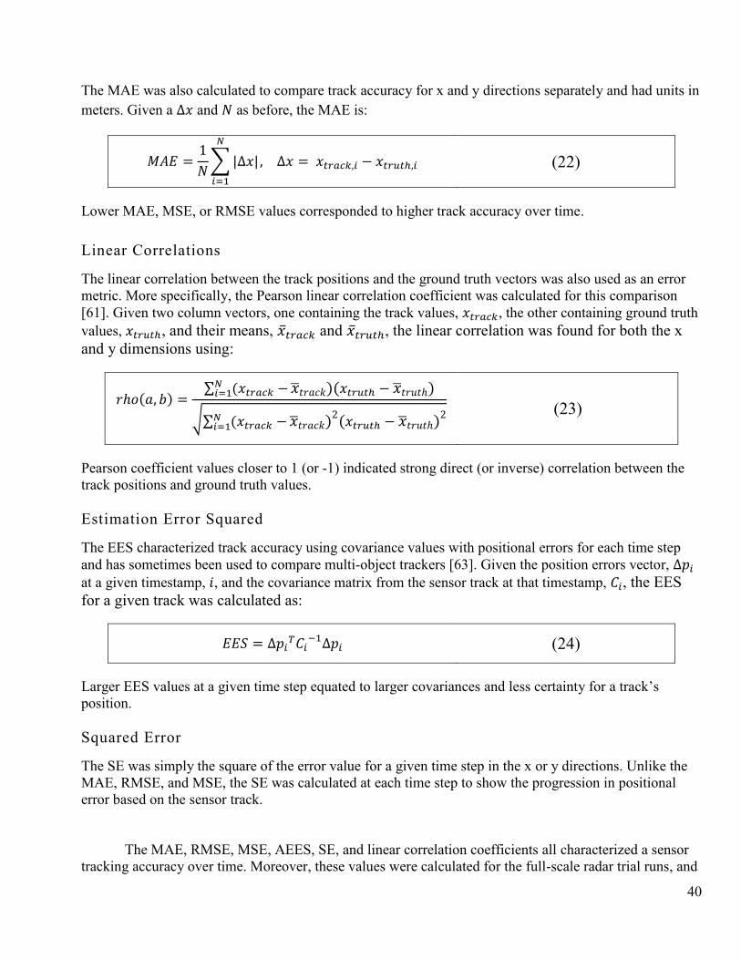
40

The MAE was also calculated to compare track accuracy for x and y directions separately and had units in

meters. Given a ∆𝑥 and 𝑁 as before, the MAE is:

𝑀𝐴𝐸 =1

𝑁∑|∆𝑥|

𝑁

𝑖=1

, ∆𝑥 = 𝑥𝑡𝑟𝑎𝑐𝑘,𝑖 − 𝑥𝑡𝑟𝑢𝑡ℎ,𝑖 (22)

Lower MAE, MSE, or RMSE values corresponded to higher track accuracy over time.

Linear Correlations

The linear correlation between the track positions and the ground truth vectors was also used as an error

metric. More specifically, the Pearson linear correlation coefficient was calculated for this comparison

[61]. Given two column vectors, one containing the track values, 𝑥𝑡𝑟𝑎𝑐𝑘, the other containing ground truth

values, 𝑥𝑡𝑟𝑢𝑡ℎ, and their means, �̅�𝑡𝑟𝑎𝑐𝑘 and �̅�𝑡𝑟𝑢𝑡ℎ, the linear correlation was found for both the x

and y dimensions using:

𝑟ℎ𝑜(𝑎, 𝑏) =∑ (𝑥𝑡𝑟𝑎𝑐𝑘 −𝑁

𝑖=1 �̅�𝑡𝑟𝑎𝑐𝑘)(𝑥𝑡𝑟𝑢𝑡ℎ − �̅�𝑡𝑟𝑢𝑡ℎ)

√∑ (𝑥𝑡𝑟𝑎𝑐𝑘 −𝑁𝑖=1 �̅�𝑡𝑟𝑎𝑐𝑘)

2(𝑥𝑡𝑟𝑢𝑡ℎ − �̅�𝑡𝑟𝑢𝑡ℎ)2

(23)

Pearson coefficient values closer to 1 (or -1) indicated strong direct (or inverse) correlation between the

track positions and ground truth values.

Estimation Error Squared

The EES characterized track accuracy using covariance values with positional errors for each time step

and has sometimes been used to compare multi-object trackers [63]. Given the position errors vector, ∆𝑝𝑖

at a given timestamp, 𝑖, and the covariance matrix from the sensor track at that timestamp, 𝐶𝑖, the EES

for a given track was calculated as:

𝐸𝐸𝑆 = ∆𝑝𝑖𝑇𝐶𝑖

−1∆𝑝𝑖 (24)

Larger EES values at a given time step equated to larger covariances and less certainty for a track’s

position.

Squared Error

The SE was simply the square of the error value for a given time step in the x or y directions. Unlike the

MAE, RMSE, and MSE, the SE was calculated at each time step to show the progression in positional

error based on the sensor track.

The MAE, RMSE, MSE, AEES, SE, and linear correlation coefficients all characterized a sensor

tracking accuracy over time. Moreover, these values were calculated for the full-scale radar trial runs, and

41

then compared to the same metrics calculated for the radar sensor in the 1/5th environment to measure the

tracking degradation. Comparisons across experimental conditions leveraged “increase factors,” which are

simply the final accuracy (i.e., after an experimental manipulation) divided by the original accuracy (i.e.,

before an experimental manipulation). The resultant value from the ratio reveals by what factor the value

has increased. For example, if the RMSE of a track increased from 0.2 in a full scale test to 0.6 in a small

scale test, the RMSE has increased by 3 times, and the increase factor is 3.

These metrics were also calculated across track fusion method to quantify the tracking accuracy

increase compared to using only the radar or only using the LiDAR sensor. Percent change between the

error metrics of the two input tracks and the error metrics of the fusion tracks was also calculated to show

the tracking accuracy increase of using fusion. Similarly, the final fusion track metrics were compared to

the original full scale radar track metrics to quantify the track fusion method’s usefulness at small scale.

Finally, there are two important caveats related to this analysis. First, the ArduSimple board self-

configured for this project provides accurate global positioning but does not provide any speed data.

Therefore, all comparison metrics could only be calculated from positions, not velocities. Second, the

small-scale environment tracking had to be directly compared to full scale tracking measurements.

Therefore, for compatibility, the track errors in the 1/5th environment were scaled by a factor of 5 before

any of the error metrics calculated. Thus, for example, errors of 1 m in the 1/5th environment would be

equated to 5 m at full-scale.

42

CHAPTER 4 – RESULTS AND DISCUSSION

With data from the trial runs recorded and sensor tracking and fusion software developed, error

metrics were calculated for each trial run. The full scale trial runs featured radar tracks compared to DGPS

ground truth values for all three vehicle maneuvers. The small scale trials featured radar tracks, LiDAR

tracks, and fusion tracks for similar vehicle maneuvers, also compared to DGPS ground truth values.

Recall that, represented in the 1/5th environment, vehicle size, vehicle speed, and driving distance were all

scaled to values at approximately 1/5th the magnitude of their full sized counterparts.

Each full scale and small scale trial produced video recordings of the sensor data and tracks plotted

against the DGPS ground truth values at each time step for visual reference. For the sensor track data,

there were three plots generated: an overall x vs y graph, an x vs. time graph, and a y vs. time graph2. The

4 error metrics (MSE, RMSE, MAE, linear correlation) were also calculated for each trial run, for both the

x and y values of the track. Additionally, graphs depicting the EES and SE as a function of time were

generated.

4.1 FULL SCALE TESTS

Straight

In the first full scale vehicle trial, the VUS drove straight away from the sensor, turned around, and drove

straight back toward the sensor. Fig. 11 shows the track position, track y-values, and track x-values

graphed against the DGPS ground truth for this trial, as well as the resulting EES. Fig 12 shows the SE

curves for both the x and y dimensions, while Table 3 shows the error metrics for the generated radar

tracks.

Diagonal

In the second full scale vehicle trial, the VUS drove diagonally away from the radar sensor, turned around,

and the drove diagonally across the radar’s FOV on the way back. Fig. 13 shows the track position, track

Y-values, and track X-values graphed against the DGPS ground truth for this trial, as well as the resulting

EES. Fig 14 shows the SE curves for both the x and y dimensions, while Table 4 shows the error metrics

for the trial run’s radar tracks.

S-turns

In the final scale vehicle trial, the VUS performed small s-turns while driving away from and back

towards the sensor. Fig. 15 shows the track position, track Y-values, and track X-values graphed against

the DGPS ground truth for this trial, as well as the resulting EES. Fig 16 shows the SE curves for both the

x and y dimensions, while Table 5 shows the error metrics for the trial run’s radar tracks. For

convenience, red dashes have been added to the lateral movement panels in Figs. 15 and 16 to highlight

the beginning of turns that the vehicle made during the S-turn maneuvers.

2 Due to environmental noise, some tracks were recorded at x values greater than 150m but with y values close to 0. This causes them to be plotted within the limits of the y vs time graph although they may be more than 100m away from the target vehicle. These tracks were considered extraneous to this analysis.

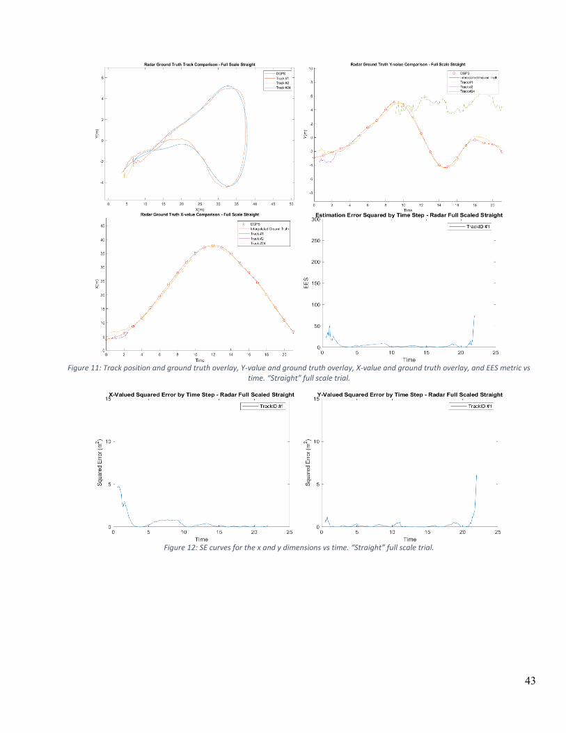
43

Figure 11: Track position and ground truth overlay, Y-value and ground truth overlay, X-value and ground truth overlay, and EES metric vs

time. “Straight” full scale trial.

Figure 12: SE curves for the x and y dimensions vs time. “Straight” full scale trial.

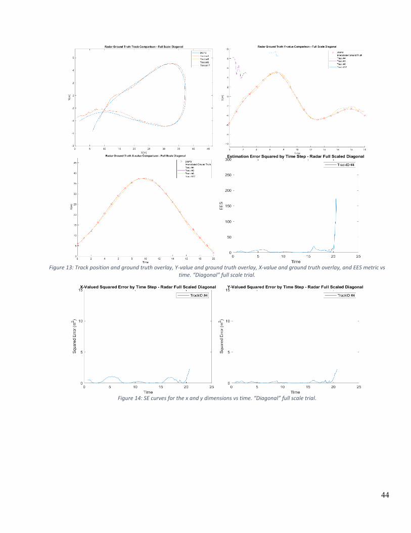
44

Figure 13: Track position and ground truth overlay, Y-value and ground truth overlay, X-value and ground truth overlay, and EES metric vs

time. “Diagonal” full scale trial.

Figure 14: SE curves for the x and y dimensions vs time. “Diagonal” full scale trial.

45

Figure 15: Track position and ground truth overlay, Y-value and ground truth overlay, X-value and ground truth overlay, and EES metric vs

time. “S-turn” full scale trial.

Figure 16: SE curves for the x and y dimensions vs time. “S-turn” full scale trial.

46

Table 3: Error metrics for full sized vehicle radar tracking, “straight” trial

Full Scale Vehicle

“Straight” Trial Run

X Y

MSE (𝑚2) 0.5078 0.2161

RMSE (𝑚) 0.7126 0.4648

MAE 0.5275 0.3378

Linear Correlation 0.9987

Table 4: Error metrics for full sized vehicle radar tracking, “diagonal” trial

Full Scale Vehicle

“Diagonal” Trial Run

X Y

MSE (𝑚2) 0.3726 0.1757

RMSE (𝑚) 0.6104 0.4192

MAE 0.5051 0.3369

Linear Correlation 0.9990

Table 5: Error metrics for full sized vehicle radar tracking, “S-turn” trial

Full Scale Vehicle

“S-turn” Trial Run

X Y

MSE (𝑚2) 3.2372 0.7122

RMSE (𝑚) 1.7992 0.8439

MAE (m) 1.5917 0.6988

Linear Correlation 0.9987

As expected, the error metrics show that the EKF with a constant velocity motion model and

added noise performs best when there are limited amounts of non-linear driving. Comparing the track

overlays, the radar tracks follow the DGPS ground truth closer when the vehicle is traveling in a straight

line. Areas where the vehicle begins to turn or stops turning often featured larger differences in the ground

truth and radar track. This is particularly evident in the “S-turns” trial (Fig. 14). Error metric values

associated with the “S-turn” trial were clearly higher than those for the “Straight” and “Diagonal”

(compare Tables 3 and 2 with Table 5). In general the graphs of the EES and SE for the “S-turn” are

higher throughout the duration of the trial than in the first two trials. However, despite the increase in

error metric values for the run, overall the EKF performed reasonably well during the challenging “S-

turn” tracking scenario. For all three trials, there was some error with the radar tracks when the vehicle

47

was within approximately 5 meters of the sensor, but accuracy seemed not to be affected at any other

range in the FOV.

With high accuracy demonstrated for the “straight” and “diagonal” trials, and successful tracking

shown across all three full scale trials, the data metrics for the full-scale were used as a benchmark for the

small scale tests.

4.2 SMALL SCALE TESTS

In addition to the radar, the small scale tests included the LiDAR and track fuser. Only the error metrics

will be shown for the remainder of this section. Associated sensor track graphs (like those that were

shown for the full scale tests) are available in Appendices A, B, and C.

Straight

The first small scale trial featured the 1/5th sized vehicle driving straight away and then back towards the

sensors. Appendix A shows all graphs for this small scale vehicle trial. Tables 6, 7 and 8 show the error

metrics for the radar, LiDAR, and fused tracks.

Table 6: Error metrics for small scaled vehicle radar tracking, “straight” trial

Small Scale Vehicle

“Straight” Trial Run, Radar

X Y

MSE (𝑚2) 5.9467 0.5344

RMSE (𝑚) 2.4386 0.7310

MAE (m) 2.2361 0.5692

Linear Correlation 0.9816 0.9426

Table 7: Error metrics for small scaled vehicle LiDAR tracking, “straight” trial

Small Scale Vehicle

“Straight” Trial Run, LiDAR

X Y

MSE (𝑚2) 9.2071 1.2424

RMSE (𝑚) 3.0343 1.1146

MAE (m) 2.6984 1.0078

Linear Correlation 0.9740 0.9622

Table 8: Error metrics for small scaled vehicle fusion tracking, “straight” trial

Small Scale Vehicle

“Straight” Trial Run, Fused Tracks

X Y

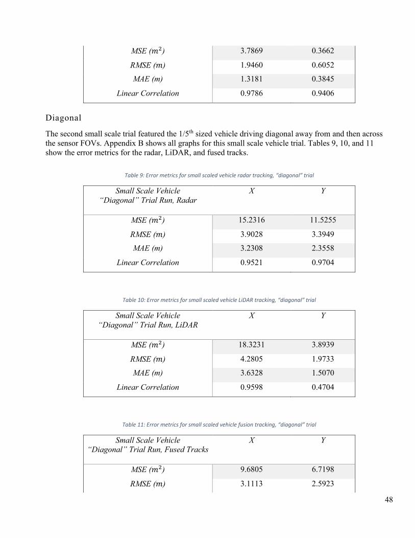
48

MSE (𝑚2) 3.7869 0.3662

RMSE (𝑚) 1.9460 0.6052

MAE (m) 1.3181 0.3845

Linear Correlation 0.9786 0.9406

Diagonal

The second small scale trial featured the 1/5th sized vehicle driving diagonal away from and then across

the sensor FOVs. Appendix B shows all graphs for this small scale vehicle trial. Tables 9, 10, and 11

show the error metrics for the radar, LiDAR, and fused tracks.

Table 9: Error metrics for small scaled vehicle radar tracking, “diagonal” trial

Small Scale Vehicle

“Diagonal” Trial Run, Radar

X Y

MSE (𝑚2) 15.2316 11.5255

RMSE (𝑚) 3.9028 3.3949

MAE (m) 3.2308 2.3558

Linear Correlation 0.9521 0.9704

Table 10: Error metrics for small scaled vehicle LiDAR tracking, “diagonal” trial

Small Scale Vehicle

“Diagonal” Trial Run, LiDAR

X Y

MSE (𝑚2) 18.3231 3.8939

RMSE (𝑚) 4.2805 1.9733

MAE (m) 3.6328 1.5070

Linear Correlation 0.9598 0.4704

Table 11: Error metrics for small scaled vehicle fusion tracking, “diagonal” trial

Small Scale Vehicle

“Diagonal” Trial Run, Fused Tracks

X Y

MSE (𝑚2) 9.6805 6.7198

RMSE (𝑚) 3.1113 2.5923

49

MAE (m) 1.9745 1.7689

Linear Correlation 0.9530 0.7040

S-turn

The third small scale trial featured the 1/5th sized vehicle driving diagonal away from and then across the

sensor FOVs. Appendix C shows all graphs for this small scale vehicle trial. Tables 12, 13, and 14 show

the error metrics for the radar, LiDAR, and fused tracks.

Table 12: Error metrics for small scaled vehicle radar tracking, “S-turn” trial

Small Scale Vehicle

“S-turn” Trial Run, Radar

X Y

MSE (𝑚2) 2.0691 2.0808

RMSE (𝑚) 1.4384 1.4425

MAE (m) 1.1773 1.2066

Linear Correlation 0.9943 0.9852

Table 13: Error metrics for small scaled vehicle LiDAR tracking, “S-turn” trial

Small Scale Vehicle

“S-turn” Trial Run, LiDAR

X Y

MSE (𝑚2) 5.7559 9.9737

RMSE (𝑚) 2.3991 3.1581

MAE (m) 1.9804 2.6277

Linear Correlation 0.9872 0.9317

Table 14: Error metrics for small scaled vehicle fusion tracking, “S-turn” trial

Small Scale Vehicle

“S-turn” Trial Run, Fused Tracks

X Y

MSE (𝑚2) 1.2485 2.7226

RMSE (𝑚) 1.1173 1.6500

MAE (m) 0.7049 1.1224

Linear Correlation 0.9924 0.9752

50

Increase factors were also calculated in order to compare the radar track error metrics from the full

scale and small scale trials (Table 15). The same increase factors were computed to compare the radar

performance at full scale and the LiDAR performance at small scale (Table 16).

Table 15: MSE, RMSE, and MAE increase factor betwee the full scale radar tracks and small scale radar tracks

Full Scale and Small Scale Radar Comparison, Increase Factor

“Straight” “Diagonal” “S-turn”

X dimension Y dimension X dimension Y dimension X dimension Y dimension

MSE (m2) 11.2 2.5 40.9 65.6 0.6 2.9

RMSE (m) 3.4 1.8 6.4 8.8 0.8 1.7

MAE (m) 4.2 1.7 6.4 7.0 0.7 1.7

Table 16: MSE, RMSE, and MAE increase factor betwee the full scale radar tracks and small scale LiDAR tracks

Full Scale Radar Small Scale LiDAR Comparison, Increase Factor

“Straight” “Diagonal” “S-turn”

X dimension Y dimension X dimension Y dimension X dimension Y dimension

MSE (m2) 18.1 5.7 49.2 22.2 1.8 14.0

RMSE (m) 4.3 2.4 7.0 4.7 1.3 3.7

MAE (m) 5.1 3.0 7.2 4.5 1.2 3.76

Comparison between the tracking metrics of the fusion technique to the sensor tracks metrics was

aided by calculation of percent change in the tracking error metrics (Table 17). The table is split into three

main columns for each small scale test, and then displays the percent change in the specified error metric

cell for the two dimensions assessed within the radar and LiDAR sensor tracks. A positive percent change

implied that the fusion approach had that smaller error when compared to the ground truth than the sensor

track by itself. A color grading has been added for emphasis and ease of interpretation.

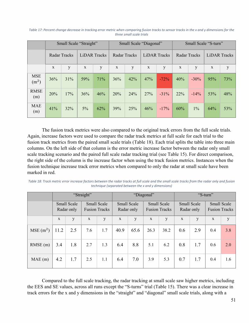
51

Table 17: Percent change decrease in tracking error metric when comparing fusion tracks to sensor tracks in the x and y dimensions for the three small scale trials

Small Scale “Straight” Small Scale “Diagonal” Small Scale “S-turn”

Radar Tracks LiDAR Tracks Radar Tracks LiDAR Tracks Radar Tracks LiDAR Tracks

x y x y x y x y x y x y

MSE

(m2) 36% 31% 59% 71% 36% 42% 47% -72% 40% -30% 95% 73%

RMSE

(m) 20% 17% 36% 46% 20% 24% 27% -31% 22% -14% 53% 48%

MAE

(m) 41% 32% 5% 62% 39% 25% 46% -17% 60% 1% 64% 53%

The fusion track metrics were also compared to the original track errors from the full scale trials.

Again, increase factors were used to compare the radar track metrics at full scale for each trial to the

fusion track metrics from the paired small scale trials (Table 18). Each trial splits the table into three main

columns. On the left side of that column is the error metric increase factor between the radar only small

scale tracking scenario and the paired full scale radar tracking trial (see Table 15). For direct comparison,

the right side of the column is the increase factor when using the track fusion metrics. Instances when the

fusion technique increase track error metrics when compared to only the radar at small scale have been

marked in red.

Table 18: Track metric error increase factors between the radar tracks at full scale and the small scale tracks from the radar only and fusion technique (separated between the x and y dimensions)

“Straight” “Diagonal” “S-turn”

Small Scale

Radar only

Small Scale

Fusion Tracks

Small Scale

Radar only

Small Scale

Fusion Tracks

Small Scale

Radar only

Small Scale

Fusion Tracks

x y x y x y x y x y x y

MSE (m2) 11.2 2.5 7.6 1.7 40.9 65.6 26.3 38.2 0.6 2.9 0.4 3.8

RMSE (m) 3.4 1.8 2.7 1.3 6.4 8.8 5.1 6.2 0.8 1.7 0.6 2.0

MAE (m) 4.2 1.7 2.5 1.1 6.4 7.0 3.9 5.3 0.7 1.7 0.4 1.6

Compared to the full scale tracking, the radar tracking at small scale saw higher metrics, including

the EES and SE values, across all runs except the “S-turns” trial (Table 15). There was a clear increase in

track errors for the x and y dimensions in the “straight” and “diagonal” small scale trials, along with a

52

slight increase in error in the y dimension of the “S-turn” small scale trials. This indicates that overall

tracking accuracy decreased when tracking in a small scale environment using the radar sensor, even

when the vehicle was performing simple maneuvers. The “Diagonal” trial posed particular problems for

the radar and saw significant error increases. The x-dimension radar track correlation with ground truth

was also the lowest for this trial. Compared to the LiDAR sensor at small scale, the radar better followed

the vehicle during maneuvers, and even successfully followed the vehicle during the S-turns despite the

high number of directional changes. On the other hand, several times the LiDAR track was lagging behind

the maneuvers of the vehicle, causing errors to increase during turning events. MSE, RMSE, and MAE

metrics were all higher for the LiDAR for all runs, when compared to the small scale radar tracks, except

in the “Diagonal” trial, where the LiDAR was more accurate in the y dimension (Table 16).

Overall, he track fuser has the lowest error metric values when compared to the radar and LiDAR

rack metrics for all the small scale trials. In all but five instances the fusion method was able to increase,

often substantially, the tracking accuracy across the MSE, RMSE, and MAE metrics. When compared to

the radar track alone, half the data metrics improved by 30% or more (Table 17). With the LiDAR, 13 out

of the 18 conditions improved by more than 30% (Table 17). Out of 18 track metric increase factor

comparisons, only twice did the fusion technique deliver overall track metrics that were worse than using

only the radar to track the vehicle at small scale (Table 18).

Computational times for the track fusion software were averaged over multiple runs for the small

scale trials. While the LiDAR clustering technique can pick out and calculate a cluster center in under

100ms, the JPDA tracker running on a 4 core Intel Core i7-4770 CPU at 3.4 GHz can only execute at

average speeds of 1.5 times the length of the recording in the native MATLAB environment. This puts the

tracker past the limits of real time requirements. However, C++ code that may be more efficient was not

generated and may potentially reduce execution time to near real-time levels.

4.3 DISCUSSION

4.3.1 FULL-SCALED TESTS

The RTS did well when tracking the full-sized vehicle, particularly during the straight and

diagonal trials. After the first few seconds of each trial, only one track was confirmed for the VUS and it

stayed with the vehicle for the remainder of the trial. For both the “straight” and “diagonal” runs, the MSE

and RMSE were well below a value of 1, meaning the average residual of the errors was less than 0.5 m in

either the x or y dimensions (Figs. 16 and 17). Video observation of the tracking recording also showed

that the radar returns, LiDAR centroids, radar tracks, and DGPS ground truth positions coincided closely

during playback of these scenarios.

In contrast with the “straight” and “diagonal” trials, however, the “S-turns” trial resulted in

substantially larger error metrics: up to six times higher in the x dimension and three times in the y

dimension. Given the pattern of vehicle movement during this trial, it is likely that the Kalman filter used

could not adapt to the non-linear movements inherent in the S-turns in order to maintain MSE, RMSE,

and MAE values that were similar in magnitude to those observed for the “straight” and “diagonal” trials.

To help visualize this, red dashes were added to the y direction track versus ground truth plot (Fig. 15) for

the full scale “S-turns” trial and to the corresponding y direction squared error graph (Fig. 16). These red

dashes mark the times when the vehicle ended one turn and initiated the next turn. The squared error

53

increased directly after the initiation of each turn, as the vehicle begins to maneuver in the opposite

direction and there is a delayed response for the Kalman filter.

It is also possible that tracking point drift may have caused some error in the “S-turns” trials.

Because the vehicle was modeled as a single point, the actual projected centroid (i.e., tracking point)

position of the vehicle could vary slightly at any time due to its position relative to the radar sensor. For

example, when the vehicle was driving away from the radar sensor, the back end of the vehicle dominated

the radar FOV. Therefore, in these situations the centroid of the radar returns will be biased toward the

rear of the vehicle. Other vehicle-to-radar orientations, however, could have caused the centroid to shift

towards either the front, right side, or left side of the vehicle in a similar fashion. When radar data are

compared to DGPS data streams, which are not subjects to this artifact, slight errors are possible –

particularly in situations where vehicle maneuvers had the potential to markedly shift the tracking point

(e.g., the “S-turns” trial). However, when the positional errors in the x and y positions were examined, the

observed effect of tracking point drift was relatively small. Both the “Diagonal” and “Straight” trials had

periods where the vehicle turned around (resulting in potential tracking point drift). The corresponding

error metric values in these conditions were consistently smaller than the “S-turns” trial throughout the

entire full scale tests. This supports the assertion that most of the tracking error observed in the S-turn

trials was due to the Kalman filter lagging in its adjustment to non-linear movements in the S-turns or to

clustering errors and not primarily to tracking point drift. It is useful to note that some ADAS algorithms

model the vehicle as a rectangular box in order to minimize the effects of tracking point error. These

algorithms tend to require in-depth extended object detection algorithms and longer processing times, and

thus were not used in this investigation.

In spite of the increase in the error metrics, however, the tracker still generated useful and

reasonable tracks through the S-turns. For example, the MAE in the x-dimension for the S-turn trial

reached a maximum of 1.5 m, which is well below the length of a normal vehicle. Other metrics, such as

the EES and SE, remained low for all of the full scale trials, including the “S-turn” trial.

Clustering errors also occasionally contributed to increases in error across full scale trials. This

was particularly observed near the onset of the full scale trials, where the vehicle was sometimes split into

two separate tracks by the radar clustering algorithm. This artifact resulted in a spurious track that was

positioned 1.5 m away from the center of the entire vehicle and contributed substantially to the overall

error. Generally, however, this issue surfaced only when the full-sized vehicle was within 5 m of the radar

sensor. Under these conditions, the vehicle would generate a large number radar returns over the vehicle

length. Normally, at distances greater than 10m, there were less than 15 radar returns from the vehicle for

any given frame. This distribution of returns was ideal for the clustering algorithm, and at these distances

the density based clustering was extremely accurate at identifying the vehicle. The issue was not observed

during the small scale tests due to the smaller size of the vehicle.

Other sources of error during the full scale trials included (1) radar reflections and (2) reduced data

accuracy at the edge of the FOV. Radar reflections, or ghost reflections, consisted of radar returns that

were primarily seen in positions directly behind the vehicle. These erroneous detections were picked up

by the sensor and were particularly hard to filter out because they include non-zero range rate values

similar to the moving vehicles. Therefore, they were sometimes clustered into possible objects. The

reflections were mostly observed when the vehicle was close to the sensor and may have been the result of

radar waves bouncing between the pillars of the vehicle and then returning to the sensor. The beginning of

some full scale trials featured these ghost reflections degrading accuracy somewhat, although their

presence posed more of a problem in the small scale sensor recordings. The end of each full scale trial

always featured the vehicle driving out of the FOV of the radar. Because the radar is less accurate in

position and range rate values at these high angles, the tracker was also less accurate during these times.

54

This is especially evident in the “Diagonal” full scale run where there was an increase in the y dimension

error at the end of the track and an increase in EES values for timestamps close to the end of the trial.

Although both of these problems, radar reflections and reduced sensor accuracy at the edge of the

FOV, were present in the collected data, the radar tracker was highly successful during the full scale tests.

This was even the case with a static radar in all trials, which tends to be a more difficult tracking scenario

than a dynamic radar situation, since there is a lack of range rate attributes for many returns in the radar

FOV. Range rate attributes can be helpful during the clustering process.

4.3.2 SMALL-SCALED TESTS

4.3.2.1 RADAR AND LIDAR ERROR METRIC COMPARISONS

Compared to the radar track metrics of the full size tests, there was a large increase in the scale-

adjusted errors associated with the radar and LiDAR tracks in the small scale test. This effect was

particularly evident in the longitudinal (x) direction, which contained most of the trial travel distance.

Although the tracker was able to follow the small scale vehicle reasonable well in the “straight” and “S-

turn” trials, there were substantial track switching and position errors in the “diagonal” trial. In the EES

and SE graphs of the radar tracks for the “Diagonal” trial, the exact point the track switches and attempts

to begin tracking the vehicle again is associated with large jumps in error values. A track switch will

always be accompanied by a large increase in error metrics, indicating the tracker is struggling to maintain

its track of the object. The increased errors are likely partially a result of increased incidence of radar

reflections during the small-scale trials. These reflections caused the clustering algorithm to incorrectly

include many of them in its cluster centroid determinations, resulting in radar centroids that were not truly

there or that were erroneously shifted in position. These extraneous radar reflections tended to be more

prevalent in objects that were close to the radar sensor. Because the small scale trials took place at

distances that were in general much closer to the radar than the full scale trial, this issue may have

contributed to the increased errors observed, especially during the “diagonal” run3.

Although the full scale trials radar tracker had its worst error metrics during the full scale “S-

turns” trial, the small scale “S-turns” trial produced error metrics comparable to the small scale “Straight”

trial. Thus, a prediction of poor performance in the small scale “S-turns” trial given the full scale results

was not accurate, the tracking algorithm was able to successfully track the vehicle through the small scale

“S-turns.” This difference in outcomes may be due to the slower speed of the small scale vehicle.

Although the small vehicle was exhibiting highly non-linear motion in this trial, the slower speed may

have allowed the radar tracker to adjust to the accelerations accurately. Also, because of slight errors in

manual driving, the small scale “S-turns” trial featured proportionally larger S-turns than the full scale S-

turns. At first glance, this would lead to theorizing that the errors would be higher in the small scale trial

because of the larger S-turns, but in reality the radar tracker was able to follow the vehicle more

accurately at small scale than full scale. This is most likely, again, due to the speed of the maneuvers.

Thus, the small deviations from the exact proportional path did not seem to play a meaningful part in

positional errors observed with the tracker. There was, however, an associated increase in the covariance

values, showcased in the EES graph for the radar sensor in the “S-turns” trials.

Video and radar cluster analysis showed that the overall number of points detected by the radar

from the VUS decreased greatly for the small scale vehicle. Rarely were there more than 4 points returned

3 The radar reflections are best observed in the tracking videos that accompany this work

55

from the small scale vehicle; comparatively, there were often at least 10 points returned from the full scale

vehicle. Density based clustering required at least two points to be present and any radar reflections seen

close to the vehicle could negatively impact clustering and increase track error metrics. Both of these

problems were observed in the small scale radar tests and likely contributed to errors in those trials,

especially for the “Diagonal” run. Additionally, unlike the full-scale tests, the small-scale tests began and

ended within the FOV of the radar (vehicle would drive out of the radar FOV at the end of the full-scale

trials. Theoretically, having the small scale vehicle start within the FOV of the sensors could have

increased errors as the small scale vehicle began to accelerate. In practice, however, there was no

evidence to suggest the radar or LiDAR tracker had increased errors at the beginning of the trials because

of the acceleration at the start of trials.

One factor that likely contributed to the surprisingly poor performance of the LiDAR during the

small scale trials was the effective cluster range. Because the LiDAR only had 16 channels, small vehicles

could slip through the sensor channels at distances greater than 10m, leading to inconsistent LiDAR

clustering and poor tracking at these distances. Typical LiDAR clusters come from the point cloud returns

of at least two channels, but many times only one channel detected the actual small scale vehicle. This

often led to less accurate clustering or failure to cluster at distances closer than 10 m. If the channel in the

LiDAR detected the vehicle with points separated by 3 to 4 cm, the RANSAC algorithm would often

include those points in the ground plane and remove them from the point cloud, effectively eliminating

them from being clustered and tracked. Stronger thresholds could be set to counteract this, but at the cost

of added run time for the LiDAR down-sampling and clustering. Using multiple LiDAR sensors or a

higher channel LiDAR could alleviate this problem in future similar efforts.

In addition, unlike radar return centroids, the LiDAR centroids do not inherently have associated

range rate values. Therefore, the JPDA EKF used with the LiDAR data had to estimate and change the

velocity on its own using only positional updates. This limitation resulted in a delayed response and

higher positional errors, particularly when the vehicle motion was non-linear, like in the “S-turns” and

“Diagonal” small scale trials. The y dimension track comparisons and SE plots demonstrate the LiDAR

positional error due to this problem.

Although less accurate than the radar, the LiDAR was still able to track the small scale vehicle in

all three tests using only basic clustering techniques. This work did not require occupancy grids like the

implementations in [18] and [23] or the multiple frame analysis and dynamic voxel grid comparison of

[26] and [27]. This lowers run time during execution and lowers algorithmic complexity, making it more

applicable to simpler scaled test beds. Also, none of the approaches in [18, 23, 26, 27] referenced low

point cloud density problems for tracked objects. Therefore, it is possible that their implementations may

also break down when faced with low point cloud density. Note, however, that most LiDAR visibility

problems would become evident at farther distances and with a less urgent need to track for system safety

if higher channel LiDARs are used.

4.3.2.2 FUSION TRACK METRICS

The collected data showed that radar tracking was generally less accurate at small scale. Due to the

limits in resolution of the radar and the increased extraneous radar reflections for nearby objects, this was

expected. In turn, the fusion method implemented was expected to increase the accuracy of tracking at

small scale using the LiDAR and radar tracks as inputs. This was indeed generally observed across trial

types and sensors.

56

Amongst the observed improvements, the “S-turn” small scale trial run benefitted the most from

the track fuser. Although the radar sensor, by itself, had relatively low errors for that trial, the fuser was

still able to improve performance. The track fuser did produce higher tracker errors in two tests than either

the LiDAR or the radar sensors working independently. This was likely due to the large difference in track

accuracies between the LiDAR and radar for those tests (e.g., see the y-dimension data in Figs. 19 and

20). The track fuser can improve upon the individual tracks, but only if the accuracies of the individual

tracks are within a certain margin. Otherwise, the fusion technique fails to improve upon either track. This

is a direct result from using the “intersection” method of estimation covariance values in the track fuser

[59]. The intersection method is the most conservative estimate of the covariance values, so if one track

has large errors or covariances, it is likely that the fused track will do so as well. In some cases, this

resulted in a fused track with an accuracy greater than one individual-sensor track but lesser than another

for periods of time. The small scale “Diagonal” trial showed this phenomenon during the track switch of

the radar. Because the EES value of the radar significantly increased during this time period, so did the

track fuser covariance values and positional accuracy. In that trial, eventually, the track was lost and

another track was detected a few time steps later.

Despite this occasional pitfall, out of 18 track metric increase factor comparisons (Table 18), only

twice did the fusion technique deliver overall track metrics that were worse than using only the radar to

track the vehicle at small scale. These two instances represented a 31% and 18% increase in error metric

increase factors for the MSE and RMSE during the “S-turn” trials. For all other instances, the increase

factor decreased when using the track fuser in the small scale environment. Just like the various

implementations of track-to-track or hybrid level fusion of [36, 37, 38, 39] that noted increased tracking

accuracy, this work showed the successful deployments of radar and LiDAR fusion at small scale, using

only the clustered centroid of point clouds as low level inputs to a LiDAR tracker. Unlike [38, 39], no

feature extraction was needed to model the vehicle in the point cloud to achieve enhanced tracking.

Additionally, unlike [36] and [39], high level fusion data was not needed to be passed back down to the

sensor level tracks to help with clustering, thus avoiding scenarios where there was increased correlation

between track inputs to the track fuser.

However, while the increase factor did decrease for the vast majority of track metrics, in many

instances it still remained quite high. The “diagonal” trial provides one such example. The track fuser

decreased the increase factor for the MSE in the x dimension by 36%, but the increase factor still

remained at 26.3 times the original MSE from the full scale test. This suggests a relationship between the

relative accuracy pairings of the sensor tracks being fused. If two sensor tracks have widely different

accuracies or covariances sustained over a period of time, the track fuser may fail to produce a track with

lower errors.

Although more accurate than using the sensor tracks alone, the track fuser and individual sensor

tracks did not operate in real time. The JPDA algorithms implemented by [50] and [51] were slow to data

associate and update tracks with given data, even from a simplified environment. Significant time is

needed to create the feasible events and then construct cost matrices for each possible measurement

pairing in the JPDA trackers. In the future, the GNN trackers described in [9] and [10] could be

implemented to produce run times within the constraints of real time execution. However, many scaled

testbeds run compute systems with dedicated GPU and CPU systems that could theoretically run some

tracking algorithms more quickly than the Intel i7 4770 CPU and MATLAB implementation that was

used herein for the tracking algorithms. This remains untested, as specialized C++ code to perform the

tracking function was not generated for this effort.

57

In general, however, this work has shown that a track fuser can increase track accuracy

substantially over time when used in a challenging tracking scenario such as a 1/5th scale environment

with clutter and highly non-linear vehicle maneuvers.

58

CHAPTER 5 – CONCLUSIONS

The aim of this work was to establish a method of including radar sensor tracking capabilities in

scaled test bed (STB) vehicles. Up to this point, radars have been largely ignored among the sensor suites

of these vehicles due to sensor limitations in a small-scaled environment. A sensor fusion approach

between radar and LiDAR was researched an implemented to address several questions regarding this

topic.

The first was to establish accurate radar tracking software at full scale as a benchmark comparison.

Common extended Kalman filter implementations and data association techniques described in Section

2.1 of this work were developed to track a moving vehicle through multiple driving maneuvers at

distances less than 75 m. Special attention was given to the constant velocity motion model and both the

JPDA and GNN data association techniques for radar tracking. Based off the trial runs of vehicle

maneuvers, it was shown that the radar tracking software was capable of overall mean absolute errors of

1.5 m or less for each trial, even in the highly non-linear “S-turn” driving scenario.

Similarly, the same tracking software was used to track a vehicle in a 1/5th scaled environment,

albeit with larger errors when accounting for the change in scale. Using the same vehicle maneuvers from

the full scale trials, the small scale trials quantified the reduction in accuracy that radar trackers face when

operating in a scaled environment. Error metrics commonly increased by factors of 3 to 10, with some

increases even as high as a factor of 49.

Attempting to restore accuracy metrics of the radar tracking software required sensor fusion

between the radar and LiDAR, two typical sensors found on many highly automated vehicle architectures.

Heavily studied, LiDAR point cloud filtering, feature extraction, and clustering was presented in Section

2.2 and adapted to calculate LiDAR centroids for the small scale data recordings in conjunction with the

radar. RANSAC algorithms removed ground plane points from the point cloud; distance based clustering

extracted clusters and centroids from each frame in under 100ms on average – no specialized feature

extraction or occupancy grid was constructed for the LiDAR object detection. The centroids served as

inputs to a separate tracker, that while successful at tracking the vehicle at small scale, often produced

error metrics that were 4 to 7 times greater errors than associated with the full scale radar tracking.

The increase in tracking accuracy was then quantifiable with the use of a track fuser between the

radar and LiDAR sensor tracks. With the high level fusion techniques described in Section 2.3, a track-to-

track GNN fuser was implemented with successful results. Tracking accuracy improved by, on average,

over 30% for all radar trials at small scale. The fused tracks resulted in increases of up to 70% for the

small scale “S-turns” trial. However, while improved, the track errors still remained 3 to 5 times higher

than the full scale radar metrics in many cases and failed to operate within the constraints of real-time

execution. This suggests that the track fuser can improve upon, but not totally restore, the tracking

accuracy of the full scale radar tracks. Despite this, video analysis shows the fuser’s ability to maintain

tracks for the duration of most driving scenarios, even those with highly non-linear maneuvers.

In lieu of real time constraints, this investigation demonstrates the ability to use radar in small

scale environments with an associated track fuser, particularly during offline analysis of sensor

recordings. The simplified LiDAR clustering and Kalman filter implementations make the approach

accessible to many scaled test bed architectures that already implement a LiDAR sensor. To maintain

radar functionality, the fused tracks can be reliably used as an input to any advanced driving assistance

system that needs radar track input.

59

5.1 LIMITATIONS

There are a number of limitations that should be addressed when adapting this work. Many revolve

around the sensor setups of the full scale and small scale trials. The radar and LiDAR sensors were

statically mounted to record data. This made it easier and efficient to transform data into the local vehicle

frame. Only the sensor locations from the center of the vehicle it was mounted on were needed, and the

locations were constant throughout the trials. For the radar, only dynamic objects had non-zero range rate

values, making it easier to pick out moving objects but harder to eliminate clutter or closely spaced

objects on the basis of radial velocity. The LiDAR itself had only 16 channels, which limited the object

detection to 20 m in the full scale trials and approximately 10 m in the small scale trials. The LiDAR was

not used in the full scale trials because of this. Thus, no full scale comparison could be made with the

LiDAR and only the statistics in the small scale trials are available for this sensor. There was also no

opportunity to quantify the fusion metrics at full scale, given the lack of LiDAR’s data input. In addition,

LiDAR trackers often use box models to track clusters, however, in this work only centroids were used to

update the LiDAR tracker. In general, box models portray more information for a track fuser to use

downstream but require adequate cluster size to function.

Other sources of limitation came from the environmental set-up for the trials. The trials were

simplified as much as possible with regards to natural clutter and number of objects. Only one moving

object, the vehicle under surveillance, was present during the trials. In addition, the trials took place on

largely open roads with no other objects in the driveable area. Busier driving conditions are normally seen

in typical driving, especially in urban scenarios. This could increase clutter and execution times for

clustering in general.

5.2 FUTURE WORK

Future work on this topic should focus on improving the radar tracking software, increasing the

number of points from the LiDAR, and decreasing run time. One possible way to improve the radar

tracking is to use a changing multiple motion model parameter for the Kalman filter. This approach would

mainly be helpful when the vehicle is turning; in other situations, a constant velocity motion model could

be applied. This could, in theory, improve accuracy if a vehicle begins to turn. Additionally, the sensor

recording systems could be adapted to a moving vehicle source to better model real life driving scenarios.

In regard to increased point cloud resolution for accurate clustering, multiple LiDARs could be

used for more sensor coverage at higher distances, or a higher channel LiDAR, such as a 32- or 64-

channel sensor, could be employed.

Decreasing run time could also be achieved by switching from a JPDA tracker to a GNN tracker

that simplifies the data association process greatly but may reduce accuracy. A quantifiable comparison

between the tracking accuracy and run time could be performed on a cost-benefit analysis basis. C++ code

could also be generated from the MATLAB functions to produce more optimized and faster code for run

time comparisons. In addition, sensitivity analysis of the parameters in the GNN trackers and JPDA

trackers could be performed in the future to develop optimal trackers.

60

REFERENCES

[1] H. Meinel, and J. Dickmann. “Automotive Radar: From Its Origin to Future Directions,”

Microwave Journal, Vol.56. 24-40, 2013.

[2] Continental AG, “ARS 408-21 Long Range Radar Sensor 77 GHz.” Continental Engineering

Services, September 2018.

[3] S. Patole, M. Torlak, D. Wang, and M. Ali. “Automotive Radars: A review of signal processing

techniques,” IEEE Signal Processing Magazine, Vol.34. 22-35, 2017.

[4] R. E. Kalman. A new approach to linear filtering and prediction problems,” Journal of basic

Engineering, Vol.82. 35-45, 1960.

[5] G. Welch, and G. Bishop. “An Introduction to the Kalman Filter,” UNC-Chapel Hill, TR 95-04,

2006.

[6] R. R. Labbe, “Kalman and Bayesian Filters in Python,” 2015, GitHub repository,

https://github.com/rlabbe/Kalman-and-Bayesian-Filters-in-Python.

[7] S. Challa, M. R. Morelande, D. Mušicki, and R. J. Evans. “Fundamentals of object tracking,”

Cambridge University Press. 2011.

[8] A. Gelb, J. F. Kasper, R. A. Nash, C. F. Price, and A. A. Sutherland. “Applied Optimal

Estimation,” M.I.T. Press. 1974.

[9] R. F. Stengel. “Optimal Control and Estimation,” Dover Publications, Inc. 1994.

[10] Y. Bar-Shalom, X. R. Li, T. Kirubarajan. “Estimation with Applications to Tracking and

Navigation: Theory Algorithms and Software,” John Wiley and Sons, Inc. 2001.

[11] D. F. Bizup and D. E. Brown. “The over-extended Kalman filter - don't use it!” Proceedings of the

Sixth International Conference of Information Fusion. 1. 40- 46.

[12] Velodyne Acoustics, Inc. “Velodyne LiDAR Puck,” 63-9229 Rev-A datasheet. 2015.

[13] R. B. Rusu and S. Cousins. “3D is here: Point Cloud Library (PCL),” IEEE International

Conference on Robotics and Automation. 2011.

[14] D. Xu and Y. Tian. “A Comprehensive Survey of Clustering Algorithms,” Annals of Data Science.

Vol2. 10. 2015.

[15] Y. Roth-Tabak, and R. Jain. “Building an Environment Model Using Depth Information,”

Computer. Vol22. 85 - 90. 1989.

[16] “Documentation: Point Cloud Compression – Octree Compression.” Pcl.org. Point Cloud Library.

2018.

[17] A. Elfes. “Using Occupancy Grids for Mobile Robot Perception and Navigation,” Computer.

Vol22. 46 - 57. 1989.

[18] H. Wang, X. Lou, Y. Cai, and L. Chen. “A 64-Line Lidar-Based Road Obstacle Sensing

Algorithm for Intelligent Vehicles,” Scientific Programming. 1-7. 2018.

[19] R. Fischler and M. Bolles. “Random Sample Consensus: A Paradigm for Model Fitting with

Applications to Image Analysis and Automated Cartography,” Communications of the ACM.

Vol24. 619-638. 1981.

[20] M. Shi, Q. Ling, Z. Yu, and J. Zhu. “Association using modified Global Nearest Neighbor in the

presence of bias,” Chinese Control Conference, CCC. 4688-4691. 2013.

[21] A. Mendes, L. C. Bento, and U. Nunes. “Multi-target detection and tracking with a laser scanner,”

IEEE Intelligent Vehicles Symposium. 796 - 801. 2004.

[22] C. Mertz, L. Navarro-Serment, R. Maclachlan, P. Rybski, A. Steinfeld, AQ. Suppé, C. Urmson, N.

Vandapel, M. Hebert, C. Thorpe, and D. Duggins. “Moving object detection with laser scanners. J.

Field Robot,” Journal of Field Robotics. Vol30. 17-43. 2013.

61

[23] A. Azim, and O. Aycard. “Detection, classification and tracking of moving objects in a 3D

environment,” IEEE Intelligent Vehicles Symposium, Proceedings. 802-807. 2012.

[24] R. Kaestner, J. Maye, Y. Pilat, and R. Siegwart. “Generative Object Detection and Tracking in 3D

Range Data,” IEEE International Conference on Robotics and Automation, Proceedings. 2012.

[25] Y. Zhou, Y. Yu, G. Lu, and S. Du. “Super-Segments Based Classification of 3D Urban Street

Scenes,” International Journal of Advanced Robotic Systems. Vol9. 2012.

[26] A. Asvadi, C. Premebida, P. Peixoto, and U. Nunes. “3D Lidar-based Static and Moving Obstacle

Detection in Driving Environments: an approach based on voxels and multi-region ground

planes,” Robotics and Autonomous Systems. Vol83. 2016.

[27] D. Xie, Y. Xu, and R. Wang. “Obstacle detection and tracking method for autonomous vehicle

based on three-dimensional LiDAR,” International Journal of Advanced Robotic Systems. Vol16.

2019.

[28] N. Kaempchen, K. Fuerstenberg, A. Skibicki, and K. Dietmayer. “Sensor Fusion for Multiple

Automotive Active Safety and Comfort Applications,” Advanced Microsystems for Automotive

Applications, 137-163. 2004.

[29] R. Aufrère, J. Gowdy, C. Mertz, C. Thorpe, C. Wang, and T. Yata. “Perception for collision

avoidance and autonomous driving,” Mechatronics. Vol13. 1149-1161. 2003.

[30] M. Mahlisch, R. Schweiger, W. Ritter, and K. Dietmayer. “Sensor fusion Using Spatio-Temporal

Aligned Video and Lidar for Improved Vehicle Detection,” IEEE Intelligent Vehicles Symposium,

Proceedings. 424 - 429. 2006.

[31] C. Premebida, P. Peixoto, U. Nunes. “Tracking and Classification of Dynamic Obstacles using

Laser Range Finder and Vision,” IEEE Workshop on Safe Navigation in Open and Dynamic

Environments. 2006.

[32] P. Wei, L. Cagle, T. Reza, J. Ball, and J. Gafford. “LiDAR and Camera Detection Fusion in a Real

Time Industrial Multi-Sensor Collision Avoidance System,” Electronics. Vol7. 2018.

[33] A. Andersson. “Offline Sensor Fusion for Multitarget Tracking using Radar and Camera

Detections,” Master’s Thesis. KTH Royale Institute of Technology, School of Computer Science

and Communication. 2017.

[34] L. Ekstrom and J. Risberg. “Sensor fusion of radar and stereo-vision for tracking moving vehicles

as extended objects,” Master’s Thesis. Chalmers University of Technology, Department of

Electrical Engineering. 2018.

[35] C. Blanc, L. Trassoudaine, Y. Guilloux, and R. Moreira. “Track to Track Fusion Method Applied

to Road Obstacle Detection,” 2004.

[36] D. Goehring, M. Wang, M. Schnurmacher, and T. Ganjineh. “Radar/Lidar sensor fusion for car-

following on highways,” 5th International Conference on Automation, Robotics and Applications.

407-412. 2011.

[37] H. Hajri and M. Rahal, Mohamed. (2018). “Real Time Lidar and Radar High-Level Fusion for

Obstacle Detection and Tracking with evaluation on a ground truth,” International Journal of

Mechanical and Mechatronics Engineering. Vol12. No8. 2018.

[38] K. Na, J. Byun, M. Roh, and B. Seo. “Fusion of multiple 2D LiDAR and RADAR for object

detection and tracking in all directions,” International Conference on Connected Vehicles and

Expo. 2014.

[39] H. Cho, Y. Seo, B. Kumar, and R. Rajkumar. “A multi-sensor fusion system for moving object

detection and tracking in urban driving environments,” IEEE International Conference on

Robotics and Automation. 2014.

[40] S. Brennan and A. G. Alleyne. “Using a scale testbed: Controller design and evaluation,” Control

Systems. Vol21. 15 - 26. 2001.

62

[41] R. Longoria, A. Al-Sharif, and C. Patil. “Scaled vehicle system dynamics and control: A case

study in anti-lock braking,” International Journal of Vehicle Autonomous Systems. Vol2. 2004.

[42] D. Katzourakis and A. Katzourakis. “Scaled Test Bed for Automotive Experiments: Evaluation of

Single Accelerometer Electronic Stability Control,” Advanced Microsystems for Automotive

Applications, pp239-257. 2008.

[43] Z. Xu, M. Wang, F. Zhang, S. Jin, J. Zhang, and X. Zhao. “PaTAVTT: A Hardware-in-the-Loop

Scaled Platform for Testing Autonomous Vehicle Trajectory Tracking,” Journal of Advanced

Transportation. 2017.

[44] M. O'Kelly, V. Sukhil, H. Abbas, J. Harkins, C. Kao, Y. Pant, R. Mangharam, D. Agarwal, M.

Behl, P. Burgio, and M. Bertogna. “F1/10: An Open-Source Autonomous Cyber-Physical

Platform.” 2019.

[45] “Qcar – Sensore-Rich Autonomous Vehicle,” Quanser.com. Quanser. 2020.

[46] “Jackal Unmanned Ground Vehicle,” Clearpathrobotics.com. Clearpath Robotics Inc. 2019.

[47] Continental AG, “Technical Product Specification: ARS430 RDI,” Continental AG – Advanced

Driver Assistance Systems Business Unit, October 2017.

[48] “Documentation: Downsampling a PointCloud using a VoxelGrid filter.” Pcl.org. Point Cloud

Library. 2018.

[49] “Taxonomy and Definitions for Terms Related to On-Road Motor Vehicle Automated Driving

Systems,” SAE International, J3016B. 2018.

[50] T. Fortmann, Y. Bar-Shalom and M. Scheffe, "Sonar tracking of multiple targets using joint

probabilistic data association," in IEEE Journal of Oceanic Engineering, vol. 8, no. 3, pp. 173-184,

July 1983.

[51] J. Fisher and D. Casasent, "Fast JPDA multitarget tracking algorithm," Applied Optics, Vol.28.

371-376. 1989

[52] B. Zhou and N. K. Bose, "Multitarget tracking in clutter: fast algorithms for data association," in

IEEE Transactions on Aerospace and Electronic Systems, Vol.29. 352-363, April 1993.

[53] D. Musicki and R. Evans, "Joint Integrated Probabilistic Data Association - JIPDA," Proceedings

of the Fifth International Conference on Information Fusion. FUSION 2002. Annapolis, MD,

USA, 2002, Vol.2. 1120-1125. 2002.

[54] “Octree2.png” by Nu is licensed under CC 3.0 Attribution Share. 2006.

[55] “Fitted Line.svg” by Msm is licensed under CC 3.0 Attribution Share. 2007.

[56] Ester, M., H.-P. Kriegel, J. Sander, and X. Xiaowei. “A density-based algorithm for discovering

clusters in large spatial databases with noise.” In Proceedings of the Second International

Conference on Knowledge Discovery in Databases and Data Mining, 226-231. Portland, OR:

AAAI Press, 1996.

[57] https://www.mathworks.com/help/fusion/ref/trackerjpda-system-object.html

[58] https://www.mathworks.com/help/fusion/ref/trackfuser-system-object.html

[59] Chee-Yee Chong, S. Mori, W. H. Barker and Kuo-Chu Chang, "Architectures and algorithms for

track association and fusion," in IEEE Aerospace and Electronic Systems Magazine, vol. 15, no. 1,

pp. 5-13, Jan. 2000.

[60] U.S. Department of Transportation (2018) “Low-Speed Automated Shuttles: State of the

Practice.” Report no. FHWA-JPO-18-692. John A. Volpe National Transportation Systems Center.

Cambridge, MA.

[61] Gibbons, J.D. Nonparametric Statistical Inference. 2nd ed. M. Dekker, 1985.

[63] Schuhmacher, B., B. -T. Vo, and B. -N. Vo. "A Consistent Metric for Performance Evaluation of

Multi-Object Filters." IEEE Transactions on Signal Processing, Vol, 56, No, 8, pp. 3447–3457,

2008.

63

APPENDIX A

SMALL SCALE “STRAIGHT” TRIAL RUN GRAPHS

Figure 17: Track position and ground truth overlay, Y-value and ground truth overlay, X-value and ground truth overlay, and EES

metric vs time. “Straight” small scale trial, radar tracks.

Figure 18: SE curves for the x and y dimensions vs time. “Straight” small scale trial, radar.

64

Figure 19: Track position and ground truth overlay, Y-value and ground truth overlay, X-value and ground truth overlay, and EES

metric vs time. “Straight” small scale trial, LiDAR tracks.

Figure 20: SE curves for the x and y dimensions vs time. “Straight” small scale trial, LiDAR.

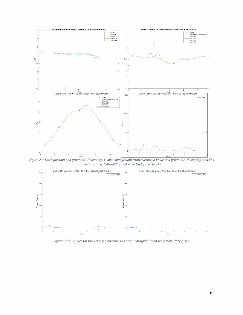
65

Figure 21: Track position and ground truth overlay, Y-value and ground truth overlay, X-value and ground truth overlay, and EES

metric vs time. “Straight” small scale trial, fused tracks.

Figure 22: SE curves for the x and y dimensions vs time. “Straight” small scale trial, track fuser.

66

APPENDIX B

SMALL SCALE “DIAGONAL” TRIAL RUN GRAPHS

Figure 23: Track position and ground truth overlay, Y-value and ground truth overlay, X-value and ground truth overlay, and EES metric vs time. “Diagonal” small scale trial, radar tracks.

Figure 24: SE curves for the x and y dimensions vs time. “Diagonal” small scale trial, radar.

67

Figure 25: Track position and ground truth overlay, Y-value and ground truth overlay, X-value and ground truth overlay, and EES metric vs time. “Diagonal” small scale trial, LiDAR tracks.

Figure 26: SE curves for the x and y dimensions vs time. “Diagonal” small scale trial, LiDAR.

68

Figure 27: Track position and ground truth overlay, Y-value and ground truth overlay, X-value and ground truth overlay, and EES

metric vs time. “Diagonal” small scale trial, fused tracks.

Figure 28: SE curves for the x and y dimensions vs time. “Diagonal” small scale trial, fused tracks.

69

APPENDIX C

SMALL SCALE “S-TURN” TRIAL RUN GRAPHS

Figure 29: Track position and ground truth overlay, Y-value and ground truth overlay, X-value and ground truth overlay, and EES

metric vs time. “S-turn” small scale trial, radar tracks.

Figure 30: SE curves for the x and y dimensions vs time. “Diagonal” small scale trial, radar.

70

Figure 31: Track position and ground truth overlay, Y-value and ground truth overlay, X-value and ground truth overlay, and EES metric vs time. “S-turn” small scale trial, LiDAR tracks.

Figure 32: SE curves for the x and y dimensions vs time. “Diagonal” small scale trial, LiDAR.

71

Figure 33: Track position and ground truth overlay, Y-value and ground truth overlay, X-value and ground truth overlay, and EES metric vs time. “S-turn” small scale trial, fused tracks.

Figure 34: SE curves for the x and y dimensions vs time. “Diagonal” small scale trial, fused tracks.

72

APPENDIX D

CONTINENTAL AUTOMOTIVE ARS 400 SERIES RADAR DATA SHEET

73

74

APPENDIX E

VELODYNE PUCK LIDAR DATA SHEET

75