
Rabier-Lectures on Topics in One Parameter Bifurcation Problems
238
Lectures on Topics In One-Parameter Bifurcation Problems By P. Rabier Tata Institute of Fundamental Research Bombay 1985
-
Upload
apostol-faliagas -
Category
Documents
-
view
217 -
download
0
Transcript of Rabier-Lectures on Topics in One Parameter Bifurcation Problems

8/2/2019 Rabier-Lectures on Topics in One Parameter Bifurcation Problems
http://slidepdf.com/reader/full/rabier-lectures-on-topics-in-one-parameter-bifurcation-problems 1/238
8/2/2019 Rabier-Lectures on Topics in One Parameter Bifurcation Problems
http://slidepdf.com/reader/full/rabier-lectures-on-topics-in-one-parameter-bifurcation-problems 2/238

8/2/2019 Rabier-Lectures on Topics in One Parameter Bifurcation Problems
http://slidepdf.com/reader/full/rabier-lectures-on-topics-in-one-parameter-bifurcation-problems 3/238
Author
P. RabierAnalyse Num´erique, Tour 55-65, 5 e etage
Universit´e Pierre et Marie Curie4, Place Jussieu
75230 Paris Cedex 05France
c Tata Institute of Fundamental Research, 1985
ISBN 3-540-13907-9 Springer-Verlag, Berlin. Heidelberg.New York. Tokyo
ISBN 0-387-13907-9 Springer-Verla, New York. Heidelberg.Berlin. Tokyo
No part of this book may be reproduced in any
form by print, microlm or any other means with-out written permission from the Tata Institute of Fundamental Research, Colaba, Bombay 400 005
Printed by M. N. Joshi at The Book Centre Limited,Sion East, Bombay 400 022 and published by H. Goetze,
Springer-Verlag, Heidelberg, West Germany
Printed In India

8/2/2019 Rabier-Lectures on Topics in One Parameter Bifurcation Problems
http://slidepdf.com/reader/full/rabier-lectures-on-topics-in-one-parameter-bifurcation-problems 4/238

8/2/2019 Rabier-Lectures on Topics in One Parameter Bifurcation Problems
http://slidepdf.com/reader/full/rabier-lectures-on-topics-in-one-parameter-bifurcation-problems 5/238
Preface
This set of lectures is intended to give a somewhat synthetic expositionfor the study of one-parameter bifurcation problems. By this, we mean
the analysis of the structure of their set of solutions through the sametype of general arguments in various situations.
Chapter I includes an introduction to one-parameter bifurcationproblems motivated by the example of linear eiqenvalue problems andstep by step generalizations lead to the suitable mathematical form. The Lyapunov-Schmidt reduction is detailed next and the chapter is com-pleted by an introduction to the mathematical method of resolution,based on the Implicit function theorem and the Morse lemma in the sim-plest cases. The result by Crandall and Rabinowitz [ 7] about bifurcation from the trivial branch at simple characteristic values is given as anexample for application.
Chapter II presents a generalization of the Morse lemma in its“weak” form to mappings from R n+ 1 into R n. A slight improvementof one degree of regularity of the curves as it can be found in the litera-ture, is proved, which allows one to include the case when the Implicitfunction theorem applies and is therefore important for the homogeneityof the exposition. The relationship with stronger versions of the Morselemma is given for the sake of completeness but will not be used in thesequel.
Chapter III shows how to apply the results of Chapter II to the studyof one-parameter bifurcation problems. Attention is conned to two
general examples. The rst one deals with problems of bifurcation fromthe trivial branch at a multiple characteristic value. A direct application
v

8/2/2019 Rabier-Lectures on Topics in One Parameter Bifurcation Problems
http://slidepdf.com/reader/full/rabier-lectures-on-topics-in-one-parameter-bifurcation-problems 6/238
vi Preface
may be possible but, for higher non-linearities, a preliminary change
of scale is necessary. The justication of this change of scale is givenat an intuitive level only, because a detailed mathematical justicationinvolves long and tedious technicalities which do not help much for un-derstandig the basic phenomena, even if they eventually provide a sat-isfactory justication for the use of Newton diagrams (which we do notuse however). The conclusions we draw are, with various additional in-formation, those of McLeod and Sattinger [ 23]. The second exampleis concerned with a problem in which no particular branch of solutionsis known a priori. It is pointed out that while the case of a simple sin-gularity is without bifurcation, bifurcation does occur in general whenthe singularity is multiple. Also, it is shown how to get further details
on the location of the curves when the results of Chapter II apply aftera suitable change of scale and how this leads at once to the distinctionbetween “turning points” and “hysteresis points” when the singularity issimple.
Chapter IV breaks with the traditional exposition of the Lyapunov-Schmidt method, of little and hazardous practical use, because its as-sumed data are not known in the applications while the imperfectionsensitivity of the method has not been evaluated (to the best of ourknowledge at least). Instead, we present a new, more general (and webelieve, more realistic) method, introduced in Rabier-El Hajji [ 33] andderived from the “almost” constructive proofs of Chapter II. Optimalrate of convergence is obtained. For the sake of brevity, the technicali-ties of §5 have been skipped but the rst four sections fully develop allthe main ideas.
Chapter V introduces a new method in the study of bifurcation prob-lems in which the nondegeneracy condition of Chapter II is not fullled.Actually, the method is new in that it is applied in this context but simi-lar techniques are classical in the desingularization of algebraic curves.We show how to nd the local zero set of a C ∞ real-valued functionof two variables (though the regularity assumption can be weakened inmost of the cases) verifying f (0) = 0, D f (0) = 0, D2 f (0) 0 but
det D2
f (0) = 0 (so that the Morse condition fails). This method is ap-plied to a problem of bifurcation from the trivial branch at a geometri-

8/2/2019 Rabier-Lectures on Topics in One Parameter Bifurcation Problems
http://slidepdf.com/reader/full/rabier-lectures-on-topics-in-one-parameter-bifurcation-problems 7/238
Preface vii
cally simple characteristic value when the nondegeneracy condition of
Crandall and Rabinowitz is not fullled (i.e. the algebraic multiplicityas > 1). The role played by the generalized null space is made clearand the result complements Krasnoselskii’s bifurcation theorem in theparticular case under consideration.
8/2/2019 Rabier-Lectures on Topics in One Parameter Bifurcation Problems
http://slidepdf.com/reader/full/rabier-lectures-on-topics-in-one-parameter-bifurcation-problems 8/238
viii Preface
Acknowledgement
I wish to thank Professor M.S. NARASIMHAN for inviting me andgiving me the opportunity to deliver these lectures at the Tata Instituteof Fundamental Research Centre, Bangalore, in July and August 1984.I am also grateful to Drs. S. KESAVAN and M. VANNINATHAN whoinitially suggested my visit.
These notes owe much to Professor S. RAGHAVAN and Dr. S. KE-SAVAN who used a lot of their own time reading the manuscript. Theyare responsible for numerous improvements in style and I am more thanthankful to them for their great help.

8/2/2019 Rabier-Lectures on Topics in One Parameter Bifurcation Problems
http://slidepdf.com/reader/full/rabier-lectures-on-topics-in-one-parameter-bifurcation-problems 9/238
Contents
Preface v
1 Introduction to One-Parameter Bifurcation Problems 11.1 Introduction . . . . . . . . . . . . . . . . . . . . . . . . 11.2 The Lyapunov-Schmidt Reduction . . . . . . . . . . . . 101.3 Introduction to the Mathematical Method...... . . . . . . 15
2 A generalization of the Morse Lemma 292.1 A Nondegeneracy Condition For......... . . . . . . . . . . 292.2 Practical Verication of the Condition ( R -N.D.). . . . . . 332.3 A Generalization of the Morse Lemma..... . . . . . . . . 402.4 Further Regularity Results. . . . . . . . . . . . . . . . . 48
2.5 A Generalization of the Strong Version..... . . . . . . . . 54
3 Applications to Some Nondegenerate problems 573.1 Equivalence of Two Lyapunov-Schmidt Reductions. . . . 583.2 Application to Problems of Bifurction..... . . . . . . . . 653.3 Application to a Problem...... . . . . . . . . . . . . . . . 85
4 An Algorithm for the Computation of the Branches 994.1 A Short Review of the Method of Chapter II. . . . . . . 1004.2 Equivalence of Each Equation with a... . . . . . . . . . . 1014.3 Convergence of the Successive Approximation Method. . 106
4.4 Description of the Algorithm. . . . . . . . . . . . . . . . 1084.5 A Generalization to the Case..... . . . . . . . . . . . . . 111
ix

8/2/2019 Rabier-Lectures on Topics in One Parameter Bifurcation Problems
http://slidepdf.com/reader/full/rabier-lectures-on-topics-in-one-parameter-bifurcation-problems 10/238
x Contents
4.6 Application to One-Parameter Problems. . . . . . . . . . 116
5 Introduction to a Desingularization Process.... 1255.1 Formulation of the Problem and Preliminaries. . . . . . . 1275.2 Desingularization by Blowing-up Procedure. . . . . . . . 1305.3 Solution Through the Implict Function.... . . . . . . . . 1355.4 Solution Through the Morse Lemma.... . . . . . . . . . . 1395.5 Iteration of the Process. . . . . . . . . . . . . . . . . . . 1465.6 Partial Results on the Intrinsic Character of the Process . 1555.7 An Analytic Proof of Krasnoselskii’s Theorem.... . . . . 1615.8 The Case of an Innite Process. . . . . . . . . . . . . . 1705.9 Concluding Remarks on Further Possible Developments. 181
Appendix 1: Practical Verication of the Conditions..... 185
Appendix 2: Complements of Chapter IV 193
8/2/2019 Rabier-Lectures on Topics in One Parameter Bifurcation Problems
http://slidepdf.com/reader/full/rabier-lectures-on-topics-in-one-parameter-bifurcation-problems 11/238
Chapter 1
Introduction toOne-Parameter BifurcationProblems
1.1 Introduction
In this, section, we introduce one-parameter bifurcation problems 1
through the example of linear eigenvalue problems. In increasing or-der of generality, they rst lead to non-linear eigenvalue problems, next,
to problems of bifurction from the trivial branch and nally to a largeclass of problems for which a general mathematical analysis can be de-veloped.
1.1a Linear Eigenvalue Problems
Let X be a real vector space. Given a linear operator L : X →X , weconsider the problem of nding the pairs ( λ, x) R × X that
x = λ Lx.
For λ = 0, x = 0 is the unique solution. For λ 0, and setting
τ = 1/λ , it is equivalent to τ x = Lx.
1
8/2/2019 Rabier-Lectures on Topics in One Parameter Bifurcation Problems
http://slidepdf.com/reader/full/rabier-lectures-on-topics-in-one-parameter-bifurcation-problems 12/238
2 1. Introduction to One-Parameter Bifurcation Problems
The values τ R such that there exists x 0 satisfying the above
equation are called eigen values of L. When λ 0, the correspondingvalue λ = 1/τ is called a characteristic value of L.
It may happen that every non-zero real number λ is a characteristic2
value of L. For instance, if X = D ′(R ) (distributions over R ) and L isthe operator Lx = x′′ D (R ). Then
x = λ x′′ ↔x(s) = e s/ √ λ .
But this is not the case in general. In what follows, we shall assumethat X is a real Banach space and that L L ( x) is compact .
From the special theory of linear operators in Banach spaces, it isknown that
(i) The characteristic values of L form a sequence λ j j≥1 with nocluster point (the sequence is nite if dim X < ∞).
(ii) For every λ R , Range ( I −λ L) is closed and dim Ker( I −λ L) =codim Range ( I −λ L) < ∞(and is greater than or equal to 1 if and only if λ = λ j for some j).
Let us now set H (λ, x) = x −λ Lx
so that the problem consists in nding the pairs ( λ, x) R ×X such that H (λ, x) = 0. The set of solutions of this equation ( zero set of H ) is theunion of the line
(λ, 0); λ R
(trivial branch ) and the set
j≥1λ j
×E j
where E j denotes the eigenspace associated with the characteristic valueλ j.
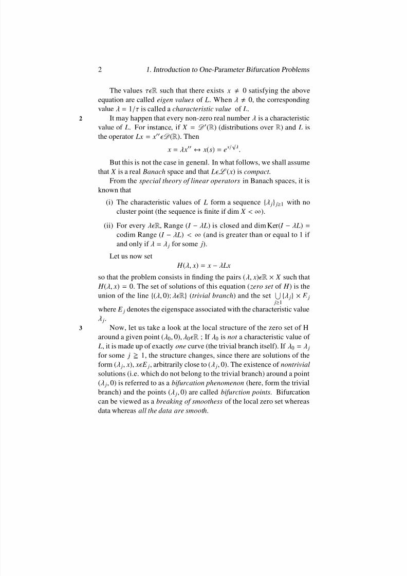
Now, let us take a look at the local structure of the zero set of H3
around a given point ( λ0 , 0), λ 0 R ; If λ0 is not a characteristic value of L, it is made up of exactly one curve (the trivial branch itself). If λ0 = λ j
for some j 1, the structure changes, since there are solutions of theform ( λ j, x), x E j, arbitrarily close to ( λ j, 0). The existence of nontrivialsolutions (i.e. which do not belong to the trivial branch) around a point(λ j, 0) is referred to as a bifurcation phenomenon (here, form the trivialbranch) and the points ( λ j, 0) are called bifurction points . Bifurcation
can be viewed as a breaking of smoothess of the local zero set whereasdata whereas all the data are smooth .

8/2/2019 Rabier-Lectures on Topics in One Parameter Bifurcation Problems
http://slidepdf.com/reader/full/rabier-lectures-on-topics-in-one-parameter-bifurcation-problems 13/238
1.1. Introduction 3
1.1b Generalization I: Problems of bifurcation from the triv-
ial branch.A natural extension is when the linear operator L is replaced by a map-ping T : X →X (nonlinear in general) such that T (0) = 0. The problembecomes: Find ( λ, x) R × X such that
x = λT ( x).
Again, the pairs ( λ, 0)λ R are always solutions of this equation ( triv-ial branch ). On the basis of the linear case, a natural question is to knowwhether there are “bifurcation points” on the trivial branch, namely so-lutions ( λ, 0) around which nontrivial solutions always exist.
Theorem 1.1 (Necessary condition) . Assume that T is di ff erentiable at 4the origin and the linear operator DT (0) L ( X ) is compact. Then anecessary condition for (λ0 , 0) to be a bifurcation point of the equation x = λT ( x) is that λ0 is a characteristic value of DT (0) .
Proof. WriteT ( x) = DT (0) ·x + (|| x||)
and let ( λ (i) , x(i)) be a sequence tending to ( λ0 , 0) with x(i) 0 and
x(i) = λ (i)T ( x(i)).
Thus,
x(i)
= λ(i)
DT (0) ·x(i)
+ 0(|| x(i)
||)Dividing by || x(i)|| 0, we get
x(i)
|| x(i)||= λ (i) DT (0) .
x(i)
|| x(i)||+ 0(1)
The sequence x(i)
|| x(i)||is bounded. Due to the compactness of the
operator DT (0), we may assume, after considering a subsequence, thatthe right hand side tends to a limit v, which is then the limit of thesequence x(i)
|| x(i) ||as well. Of course, v 0 and making i tend to + ∞, we
ndv = λ0 DT (0)
·v,
which shows that λ0 is a characteristic value of DT (0).
8/2/2019 Rabier-Lectures on Topics in One Parameter Bifurcation Problems
http://slidepdf.com/reader/full/rabier-lectures-on-topics-in-one-parameter-bifurcation-problems 14/238
4 1. Introduction to One-Parameter Bifurcation Problems
Remark 1.1. As T is nonlinear (a very general assumption !) it is im-5
possible, without additional hypotheses to expect more than local results(in contrast to the linear case where global results are obtained).
Remark 1.2. Even when λ0 is a characteristic value of DT (0), bifurca-tion is not ensured. For instance, take X = R 2 and x = ( x1, x2) with
T ( x1 , x2 ) = x1 + x3
2
x2 −x31
.
Here, DT (0) = I , whose unique characteristic value is λ1 = 1. Theequation x = λT ( x) becomes
x1 = λ x1 + λ x32 ,
x2 = λ x2 −λ x31 .
Multiplying the rst equation by x2 and the second one by − x1 andadding the two we get λ( x4
1 + x42) = 0. Hence for λ around 1, we must
have x = 0 and no bifurcation occurs.
These nonlinear eigenvalue problems are particular cases of a moregeneral class called problems of bifurcation from the trivial branch . Bydenition , a problem of bifurcation from the trivial branch is an equationof the form
x = λ Lx
−φ(λ, x),
where L L ( X ) and φ is a nonlinear operator from X to itself satisfying6
φ(λ, 0) = 0 for λ R , (1.1)
φ(λ, x) = 0(|| x||), (1.2)
for x around the origin, uniformly with respect to λ on bounded intervals .It is equivalent to saying that a problem of bifurcation from the trivialbranch consists in nding the zero set of the mapping
H (λ, x) = x −λ Lx + φ(λ, x)
From our assumptions, the pairs ( λ, 0), λ R are all in the zero set of H (trivial branch ). Note, however, that our denition does not include
8/2/2019 Rabier-Lectures on Topics in One Parameter Bifurcation Problems
http://slidepdf.com/reader/full/rabier-lectures-on-topics-in-one-parameter-bifurcation-problems 15/238
1.1. Introduction 5
all mappings having the trivial branch in their zero set. Two reasons
motivate our denition. First, problems of this type are common in theliterature, for they correspond to many physical examples. Secondly,from a mathematical stand-point, their properties allow us to make ageneral study of their zero set. In particular, when L is compact , a proof similar to that of theorem 1.1 shows that λ0 needs to be characteristicvalue of L for (λ0 , 0) to be a bifurcation point. Actually, by writing theTaylor expansion of T about the origin
T ( x) = DT (0) ·x + R( x),
with R( x) = 0(|| x||), it is clear that nonlinear eigenvalue problems area particular case of problems of bifurcation from the trivial branch inwhich L = DT (0) and φ(λ, x) = −λ R( x).
The most famous result about problems of bifurction from the trivial 7
branch is a partial converse of Theorem 1.1 due to Kranoselskii.
Theorem 1.2 (Krasnoselskii) . Assume that L is compact and λ0 is acharacteristic value of L with odd algebraic multiplicity, Then (λ0 , 0) isa bifurcation point (i.e. there are solutions (λ, x) R × X −0of H (λ, x) =0 arbitrarily close to (λ0 , 0)).
The proof of Theorem 1.2 is based on topological degree argumentsand will not be given here (cf. [ 19], [27]). It is a very general result but
it does not provide any information on the structure of the zero set of H near ( λ0 , 0), a question we shall be essentially interested in, throughoutthese notes.
COMMENT 1.1. (Algebraic and geometric multiplicity of a character-istic value): Let L be compact. Given a characteristic value λ0 of L,it is well-known that the space Ker( I −λ0 L) is nite dimensional. Itsdimension is called the geometric multiplicity of λ0.
The spectral theory of compact operators in Banach spaces (see e.g.[9]) provides us with additional information; namely, there is an integerr
≥1 such that
(i) dim Ker( I −λ0 L)r < ∞,

8/2/2019 Rabier-Lectures on Topics in One Parameter Bifurcation Problems
http://slidepdf.com/reader/full/rabier-lectures-on-topics-in-one-parameter-bifurcation-problems 16/238
6 1. Introduction to One-Parameter Bifurcation Problems
(ii) X = Ker( I −λ0 L)r Range ( I −λ0 L)r .
In addition, r is characterized by8
Ker( I −λ0 L)r ′ = Ker( I −λ0 L)r for every r ′ ≥r .
The dimension of the space Ker( I −λ0 L)r is called the algebraicmultiplicity of λ0 . The algebraic multiplicity of λ0 is always greaterholds if an only if r = 1. If so, it follows from property (ii) that
X = Ker( I −λ0 L) Range ( I −λ0 L).
A typical example of this situation is when X is a Hilbert space and L is self-adjoint .
COMMENT 1.2. In particular, Krasnoselskii’s theorem applied whenr = 1 and dim Ker( I −λ0 L) = 1. For instance, this happens when Lis the inverse of a second order elliptic linear operator associated withsuitable boundary conditions and λ0 is the “rst” characteristic value of L; this result is strongly related to the maximum principle through theKrein-Rutman theorem. (See e. g. [ 20, 35]).
COMMENT 1.3. For future use, note that the mapping φ is diff eren-tiable with respect to the x variable at the origin with
D xφ(λ, 0) = 0 for every λ R , (1.3)
as it follows from ( 1.2 ).
EXAMPLES. The most important examples of problems of bifurcationfrom the trivial branch came from nonlinear partial di ff erential equa-tions. For instance, let us consider the model problem9
− u + λu ±uk = 0 in Ω ,
u H 10 (Ω ),
where Ω is a bounded open subset of R N and k ≥2 is an integer.

8/2/2019 Rabier-Lectures on Topics in One Parameter Bifurcation Problems
http://slidepdf.com/reader/full/rabier-lectures-on-topics-in-one-parameter-bifurcation-problems 17/238
1.1. Introduction 7
Under general assumptions on the boundary ∂Ω of Ω , it follows
from the Sobolev embedding theorems that uk
H −1(Ω ) for k ≤
N + 2 N −2 if
N > 2, any 1 ≤k < + ∞for N = 1 and N = 2.Denoting by L L ( H −1 (Ω ), H 10 (Ω )) the inverse of the operatoe − ,
the problem becomes equivalent to
u −λ Lu + L(uk ) = 0,
u H 10 (Ω ).
Note that the restriction of L to the space H 10 (Ω ) is compact and themapping
u H 10 (Ω )
→Luk H 10 (Ω)
is of class C ∞. In this example, the nonlinearity uk can be replacedby F (u) (respectively F (λ, u)) where F (u)( x) = f ( x, u( x)) (respectivelyF (λ, u)( x) = f (λ, x, u( x))) and f is a Carath´ eodory function satisfyingsome suitable growth conditions with respect to the second (respectivelythird) variable (see eg. Krasnoselskii [ 19], Rabier [ 30]).
Another example with a non-local nonlinearity is given by the von 10
Karman equations for the study of the buckling of thin plates. The prob-lem reads: Find u such that
u −λ Lu + C (u) = 0,
u H 20 (ω),
where ω is an open bounded subset of the plane R 2, L L ( H 20 (ω)) iscompact and C is a “cubic” nonlinear operator. The operator L takesinto account the distribution of lateral forces along the boundary ∂ω , theintensity of these forces being proportional to the scalar λ . For “small”values of λ , the only solution is u = 0 but, beyond a certain critical value,nonzero solutions appear: this corresponds to the (physically observed)fact that the plate jumps out of its for su fficiently “large” λ (see e. g.Berger [ 1] Ciarlet-Rabier [ 6]).
Coming back to the general case, our aim is to give as precise a
description as possible of the sero set of H around the point ( λ0 , 0).Assuming L is compact, we already know the answer when λ0 is not a

8/2/2019 Rabier-Lectures on Topics in One Parameter Bifurcation Problems
http://slidepdf.com/reader/full/rabier-lectures-on-topics-in-one-parameter-bifurcation-problems 18/238
8 1. Introduction to One-Parameter Bifurcation Problems
characteristic value of L: the zero set coincides with the trivial branch.
In any case, it is convenient to shift the origin and set
λ = λ0 + µ (1.4)
Γ( µ, x) = φ(λ0 + µ, x) (1.5)
so that the problem amounts to nding the zero set around the origin11
(abbreviated as local zero set ) of the mapping
G ( µ, x) = x −(λ0 + µ) Lx + Γ ( µ, x) (1.6)
Note that the mapping Γ veries the properties
Γ( µ, 0) = 0 for every µ R , (1.7)
Γ( µ, x) = 0(|| x||), (1.8)
around the origin, uniformly with respect to µ on bounded intervals . Inparticular, Γ is diff erentiable with respect to the x-variable and
D xΓ( µ, 0) = 0 for every µ R . (1.9)
1.1c GENERALIZATION II :
Let us consider a problem of bifurcation from the trivial branch with
compact operator L L ( X ), put under the form G ( µ, x) = 0 after xingthe real number λ0 as described above. From ( 1.7)
D µΓ(0) = 0. (1.10)
Together with ( 1.9 ), we see that the (global) derivative DG (0) is themapping
( µ, x) R × X →( I −λ0 L) x X . (1.11)
Hence
Ker DG (0) = R
×Ker( I
−λ0 L), (1.12)
RangeDG (0) = Range ( I −λ0 L). (1.13)

8/2/2019 Rabier-Lectures on Topics in One Parameter Bifurcation Problems
http://slidepdf.com/reader/full/rabier-lectures-on-topics-in-one-parameter-bifurcation-problems 19/238
1.1. Introduction 9
As a result, Range Dg (0) is closed and dim Ker DG (0) = codim12
RangeDG (0) + 1 < ∞(≥1, if and only if λ0 is a characteristic value of L). In other words, DG (0) is a Fredholm operator with index 1. Recallthat a linear operator A from a Banach space X to a Banach space Y issaid to be a Fredholm operator if
(i) Range A is closed,
(ii) dim ker A < ∞, codim Range A < ∞.
In this case, the di ff erence
dim Ker A
−codimRangeA
is called the index of A. For the denition and further properties of Fredholm operators, see Kato [ 17] or Schecter [ 36].
Remark 1.3. One should relate the fact that the index of DG (0) is 1 tothe fact that the parameter µ is one-dimensional. This will be made moreclear in Remark 2.2 later.
Although the parameter µ has often a physical signicance (endhence must be distinguished from the variable x for physical reasons), itis not always desirable to let it play a particular role in the mathematicalapproach of the problem.
The suitable general mathematical framework is as follows:Let there be given two real Banach spaces X and Y and let G : X →
Y be a mapping satisfying the conditions 13
G (0) = 0 (1.14)
G is diff erentiable at the origin , (1.15)
DG (0) is a Fredholm operator with index 1. (1.16)
Naturally, G need not be dened everywhere, but in a neighbour-hood of the origin only. However, for notational convenience, we shall
repeatedly make such an abuse of notation in the future, without furthermention.

8/2/2019 Rabier-Lectures on Topics in One Parameter Bifurcation Problems
http://slidepdf.com/reader/full/rabier-lectures-on-topics-in-one-parameter-bifurcation-problems 20/238
10 1. Introduction to One-Parameter Bifurcation Problems
In our previous example of problems of bifurcation from the trivial
branch, one has X = R ×X , Y = X and G ( µ, 0) = 0 for µ R . None of these assumptions is required here. In particular, nothing ensures thatthe trivial branch is in the local zero set of G . As a matter of fact, nobranch of solutions (trivial or not) is supposed to be known a priori .
The rst step of the study consists in performing the Lyapunov-Schmidt reduction allowing us to reduce the problem to a nite dimen-sional one and this will be done in the next section.
1.2 The Lyapunov-Schmidt Reduction
Let X and Y be two real Banach spaces and G : X
→Y a mapping of
class C m, m ≥1 verifying ( 1.14) - (1.16 ). Let us set
X 1 = Ker DG (0) , (2.1)
Y 2 = RangeDG (0). (2.2)
14
By hypothesis, Y 2 has nite codimension n ≥ 0 as X 1 has nitedimension n + 1. Let X 2 and Y 1 be two topological complements of X 1and Y respectively.
Remark 2.1. ( Existence of topological complements ) From the Hahn-
Banach theorem, each one-dimensional subspace of X has a topologicalcomplement. Then, each nite dimensional subspace of X (direct sumof a nite number of one-dimensional subspaces) has a topological com-plement (the intersection of the complements of these one-dimensionalsubspaces). In particular, X 1 has a topological complement. Next, theexistence of a topological complement of Y 2 is due to the fact that Y 2is closed with nite codimension. Any (nite-dimensional) algebraiccomplement of Y 2 is closed and hence is also a topological complement.Details are given for instance, in Brezis [ 4].
Thus we can write
X = X 1 X 2 (2.3)

8/2/2019 Rabier-Lectures on Topics in One Parameter Bifurcation Problems
http://slidepdf.com/reader/full/rabier-lectures-on-topics-in-one-parameter-bifurcation-problems 21/238
1.2. The Lyapunov-Schmidt Reduction 11
Y = Y 1 Y 2. (2.4)
Let Q1 and Q2 denote the (continuous) projection operators onto Y 1and Y 2 respectively. On the other hand, for every x X , set
x = x1 + x2 , x1 X 1 , x2 X 2 .
With this notation, the equation G ( x) = 0 goes over into the system
Q1G ( x1 + x2) = 0 Y 1 , (2.5)
Q2G ( x1 + x2) = 0 Y 2 , (2.6)
15
Now, from our assumptions, one has
DG (0)| X 2 I som ( X 2 , Y 2). (2.7)
Indeed, DG (0)| X 2 is clearly one-to-one, onto (by denition of X 2 andY 2) and continuous. As Y 2 is closed in Y, it is a Banach space by itself and the result follows from the open mapping theorem . Thus equation(2.6) is solved in a neighbourhood of the origin by
x2 = ( x1)(0) = 0
where : X 1 → X 2 is a uniquely determined C m mapping (Implicitfunction theorem). After substituting in the rst equation, we nd thereduced equation
Q1G ( x1 + ( x1)) = 0 Y 1 , (2.8)
equivalent to the original equation : x X , G ( x) = 0, around the origin.From now on, we drop the index “1” in the notation of the generic ele-ment of the space X 1. The mapping
x X 1 →f ( x) = Q1G ( x + ( x)) Y 1 , (2.9)

8/2/2019 Rabier-Lectures on Topics in One Parameter Bifurcation Problems
http://slidepdf.com/reader/full/rabier-lectures-on-topics-in-one-parameter-bifurcation-problems 22/238
12 1. Introduction to One-Parameter Bifurcation Problems
whose local zero set is made up of the solution of the reduced equation
(2.8) is called the reduced mapping (note of course that f veries f (0) =0).
Therefore, we have reduced the problem of nding the local zero 16
set of G to nding the local zero set of the reduced mapping f in (2.9) ,which is of class C m from a neighbouhood of the origina in the ( n + 1)-dimensional spcae X 1 into the n-dimensional space Y 1.
Remark 2.2. More generally, assume DG (0) is a Fredhlom operatorwith index p ≥1. The same process works; we end up with a reducedmappinhy from the space X 1((n + p)-dimensional) into the space Y 1(n-dimensional), so that p can be thought of as the number of “free” real
variables (cf. Remark 1.3 ).
Two Simple Properties.The derivative at the origin of the reduced mapping f(cf. ( 2.9 )) is
immediately found to be
Q1 DG (0)( I x1 + D (0)) .
But Q1 DG (0) = 0, by the denition of the space Y 1 , so that
D f (0) = 0 (2.10)
Next, from the characterization of the function and by implict dif-ferentiation, we get
Q2 DG (0)( I X 1+ D (0)) = 0.
In other words, since Q2 DG (0) = DG (0) by a denition of the spaceY 2 and since X 1 = Ker DG (0),
DG (0) · D (0) = − DG (0) · I X 1= 0 (2.11)
On the other hand, the function takes its values in the space so that17
D (0) L ( X 1 , X 2),
8/2/2019 Rabier-Lectures on Topics in One Parameter Bifurcation Problems
http://slidepdf.com/reader/full/rabier-lectures-on-topics-in-one-parameter-bifurcation-problems 23/238
1.2. The Lyapunov-Schmidt Reduction 13
and the relation ( 2.11) can be written as
DG (0)| X 2 · D (0) = 0.
Thus, form ( 2.7) D (0) = 0. (2.12)
The Lyapunov-Schmidt reduction in the case of problems of bifur-cation from the trivial branch.
In our examples later, we shall consider the case of problems of bifurcation from the trivial branch. This is the reason why we are goingto examine the form taken by the Lyapunov-Schmidt reduction in this
context. Of course, this is simply a particular case of the general methodpreviously described.
Let X = Y and consider a problem of bifurcation from the trivialbranch in the form G ( µ, x) = 0 after xing the real number λ0 . As weobserved earlier,
X 1 = Ker DG (0) = R ×Ker( I −λ0 L), (2.13)
Y 2 = RangeDG (0) = Range ( I −λ0 L). (2.14)
Setting X 1 = Ker( I −λ0 L), (2.15)
this becomes 18
X 1 = R ×X 1, (2.16)
so that any element x1 X 1 can be identied with a pair ( µ, x1) R ×X 1 .Thus given a topological complement X 2 of X 1 in the space X, we canmake the choice
X 2 = 0 × X 2 . (2.17)
Note that not every complement of X 1 in R × X is of the form (2.17 ).Nevertheless, such a choice is “standard” in the literature devoted toproblems of bifurcation from the trivial branch. Writing each element
x X as a sum x = x1 + x2 , x X 1 , x2 X 2 ,
8/2/2019 Rabier-Lectures on Topics in One Parameter Bifurcation Problems
http://slidepdf.com/reader/full/rabier-lectures-on-topics-in-one-parameter-bifurcation-problems 24/238
8/2/2019 Rabier-Lectures on Topics in One Parameter Bifurcation Problems
http://slidepdf.com/reader/full/rabier-lectures-on-topics-in-one-parameter-bifurcation-problems 25/238
1.3. Introduction to the Mathematical Method...... 15
1.3 Introduction to the Mathematical Method of
Resolution (Implicit Function Theorem andMorse Lemma).
Since f (0) = 0, the rst natural tool we can think of, for nding the localzero set of f , is the Implict function theorem . But we already saw that D f (0) = 0. Hence the Implict function theorem can be applied whenY 1 = 0(i.e., n = 0) only. In other words, one must have Y 2 = Y sothat DG (0) is onto . If so, the reduced mapping f vanishes identicallyand the problem has actually already been solved while performing theLyapunov-Schmidt reduction: the local zero set of G is given by thegraph of the mapping , that is to say, the curve
x X 1 → x + ( x) X .
20
The reader would have noticed that since DG (0) is onto, the Lya-punov - Schmidt reduction amounts to applying the Implict functiontheorem to the original problem. There is more to say about this ap-parently obvious situation. Let us come back to the case when the pa-rameter µ is explicitly mentioned in the expression for G (for physicalreasons for instance), namely X = R ×X and G = G ( µ, x). Then, forevery ( µ, x) R
× X , we have
DG (0) ·( µ, x) = µ D µG (0) + D xG (0) ·x (3.1)
and there are two possibilities for DG (0) to be onto; either
D xG (0) is onto , (3.2)
or
codim Range D xG (0) = 1 and D µG (0) Range D xG (0) . (3.3)
We shall X 1 = Ker D xG (0) .

8/2/2019 Rabier-Lectures on Topics in One Parameter Bifurcation Problems
http://slidepdf.com/reader/full/rabier-lectures-on-topics-in-one-parameter-bifurcation-problems 26/238
16 1. Introduction to One-Parameter Bifurcation Problems
When condition (3.2 ) is fullled, there, is an element ξ X such that
D xG (0) · ξ = − D µG (0) .
Hence, DG (0) is the linear mapping
( µ, x) R × X →D xG (0) ·( x− µξ ) Y
and it follows that21
X 1 = Ker DG (0) = ( µ, x) R × X , x − µξ X 1=
= ( µ, x) R × X , x = µξ + x1 , x1 X 1=
= R µ(1, ξ ) (
0
× X 1),
where R µ denotes the real line with generic variable µ. As dim X 1 = 1,we must have X 1 = 0(i.e. Ker D xG (0) = 0) and D xG (0) is then anisomorphism (in particular, ξ is unique). Thus
X 1 = R µ(1, ξ ),
a relation showing that the local zero set of G is parametrized by µ (SeeFigure 3.1 below)
Figure 3.1: “regular point”
In this case, the origin is referred to as a “regular point” . It is im-mediately checked that this is what happens in problems of bifurcation

8/2/2019 Rabier-Lectures on Topics in One Parameter Bifurcation Problems
http://slidepdf.com/reader/full/rabier-lectures-on-topics-in-one-parameter-bifurcation-problems 27/238
1.3. Introduction to the Mathematical Method...... 17
from the trivial branch when λ0 is not a characteristic value of L. To
sum up, in the rst case, the physical parameter µ can also be used as amathematical parameter for the parametrization of the local zero set of 22
G . The situtaion is di ff erent when ( 3.3 ) holds instead of ( 3.2 ). We canwrite
Y = R D µG (0) RangeD xG (0),
whereas
X 1 = Ker DG (0) = 0 ×Ker D xG (0) = 0 × X 1 .
Since dim X 1 = 1, we nd dim X 1 = 1 and the local zero set of G isa curve parametrized by x1 X 1 . It has a “vertical” tangent at the origin,namely
0
× X
1. Two typical situations are as follows:
''hysteresis point''''turning point''
Figure 3.2:
Remark 3.1. From a geometric point of view, there is no di ff erences be-tween a “regular point”, a “turning point” or a “hysteresis point”, sincethe last two become “regular” after a change of coordinates. But thereis a diff erence in the number of solutions of the equation G ( µ, x) = 0 asthe parameter µ changes sign.
EXAMPLE. Given an element y0 Y , let us consider the equation 23
F ( x) = µY 0 (3.4)
where F : X →Y is a mapping of class C m
(m ≥1) such that F (0) = 0.Setting G ( µ, x) = F ( x) − µ y0 , we are in the rst case (i.e. D xG (0) is onto

8/2/2019 Rabier-Lectures on Topics in One Parameter Bifurcation Problems
http://slidepdf.com/reader/full/rabier-lectures-on-topics-in-one-parameter-bifurcation-problems 28/238
18 1. Introduction to One-Parameter Bifurcation Problems
) if D xF (0) is onto and the solutions are given by
x = x( µ), x(0) = 0,
where x(·) is a mapping of class C m around the origin. Now, if codimRange D xF (0) = 1 and y0 Range D xF (0), we are in the second case.The curve of solutions has a vertical tangent at the origin and it is notparametrized by µ; as it follows from the above, a “natural” parameteris the one-dimensional variable of the space X 1 = Ker D xF (0) ≥1 and y0 Range D xF (0), no conclusion can be drawn as yet.
We shall now examine the case n = 1. Here the main tool will bethe Morse lemma , of which we shall give two equivalent formulations.
Theorem 3.1. (Morse lemma : “strong” version) 1 : Let f be a mappingof class C m, m ≥2 on a neighbourhood of the origin in R 2 with valuesin R , such that
f (0) = 0.
D f (0) = 0,
24
det D 2 f (0) 0 (Morse condition).
Then, there is an origin-preserving C m−1 local di ff eomorphism φ in R 2
with D φ(0) = I which transforms the local zero set of the quadratic form
ξ R 2→D2 f (0) .( ξ )2 R ,
into the local zero set of f . Moreover, φ is C m away from the origin.
Theorem 3.1’. (Morse lemma, “weak” version): Let f be a mapping of class C m, m ≥2 on a neighbourhood of the origina in R 2 with values inR , verifying
f (0) = 0,
D f (0) = 0,
1There is an veen stronger version that we shall, however, not use here.

8/2/2019 Rabier-Lectures on Topics in One Parameter Bifurcation Problems
http://slidepdf.com/reader/full/rabier-lectures-on-topics-in-one-parameter-bifurcation-problems 29/238
1.3. Introduction to the Mathematical Method...... 19
detD 2 f (0) 0( Morse condition ).
Then, the local zero set of f reduces to the origin if det D 2 f (0) > 0and is made up of two curves of class C m−1 if det D 2 f (0) < 0. Moreover,these curves are of class C m away from the origin and each of them istangent to a di ff erent one from among the two lines of the zero set of thequadratic form
ξ R 2 →D2 f (0) ·( ξ )2 R ,
at the origin.
NOTE : We say that the curves intersect transversally at the origin. 25
COMMENT 3.1. By det D2 f (0), we mean the determinant of the 2 ×2matrix representing the second derivative of f at the origin for a givenbasis of R 2 . Of course, this determinant depends on the basis (becausethe partial derivatives of f do) but its signs does not (the proof of thisassertion is simple and is left to the reader): the assumptions of Theorem3.1 and 3.1 ′ are intrinsically linked to f . In short, we shall say that thequadratic form D2 f (0) ·( ξ )2 is non-degenerate.
COMMENT 3.2. Theorem 3.1 implies Theorem 3.1 ′, since the localzero set of the quadratic form
ξ R 2 →D2 f (0) ·( ξ )2 R ,
reduces to the origin if det D2 f (0) > 0 (the quadratic form is then pos-itive or negative denite) and is made up of exactly two distinct lines if det D2 f (0) < 0. If so, the local zero set of f is the image of these twolines through the di ff eomorphism φ: it is then made up of two curveswhose tangents at the origin are the images of the two lines in questionthrough the linear isomorphism Dφ(0) = I . We shall prove Theorem 3.1 ′and that it implies Theorem 3.1 ′ in the next chapter, in a more generalframe work.

8/2/2019 Rabier-Lectures on Topics in One Parameter Bifurcation Problems
http://slidepdf.com/reader/full/rabier-lectures-on-topics-in-one-parameter-bifurcation-problems 30/238
20 1. Introduction to One-Parameter Bifurcation Problems
(i) (ii)
Figure 3.3:
26
COMMENT 3.3. Theorem 3.1 has a generalization to mappings fromR n+ 1 →R , n ≥1. It is generally stated assuming f C m , m ≥3 and thediff eomorphism φ is shown to be of class C m−2 only (as in Nirenberg[27]). This improved version is due to Kuiper [ 21]. Innite dimensionalversions (cf. [ 14, 28, 41]) are also available in this direction.
COMMENT 3.4. In contrast, Theorem 3.1 ′ has a generalization to map-ping from R n+ 1 →R n, which we shall prove in the next chapter. Thiswill be a basic tool in Chapter 3 where we study some general one-parameter problems.
Remark 3.2. There is also a generalization of the strong version to map-27
ping from R n+ p →R n , p ≥1 at the expense of losing some regularity atthe origin (cf. [ 5]).
Application-rst results. Assume n = 1 in the Lyapunov-Schmidtreduction and let f denote the reduced mapping. Since dim X 1 = n +1 = 2, dim Y 1 = n = 1 and the hypotheses of the Morse lemma areindependent of the system of coordinates , we can identify X 1 with R 2 , Y 1with R so that f becomes a mapping from a neighbourhood of the originin R 2 with values in R . The conditions ; f (0) = 0, D f (0) = 0 are
automatically fullled (cf. (2.10 )). If, in addtion, det D2
f (0) 0 (whichrequires G to be of class C 2 at least) the structure of the local zero set of

8/2/2019 Rabier-Lectures on Topics in One Parameter Bifurcation Problems
http://slidepdf.com/reader/full/rabier-lectures-on-topics-in-one-parameter-bifurcation-problems 31/238

8/2/2019 Rabier-Lectures on Topics in One Parameter Bifurcation Problems
http://slidepdf.com/reader/full/rabier-lectures-on-topics-in-one-parameter-bifurcation-problems 32/238
22 1. Introduction to One-Parameter Bifurcation Problems
D f (0) = 0,
such that the linear form D 2 f (0) · ξ L (R 2, R ) is onto for every ˜ ξ R 2 −0with D 2 f (0) ·( ˜ ξ )2 = 0. Then the local zero set od the quadratic29
form D 2 f (0) ·( ξ )2 consists of exactly 0 or 2 real lines (depending on thesign of det D 2 f (0)) and the local zero step of f is made up of the samenumber of C m−1 curves through the origin. Moreover, these curves are of class C m away from the origin and each of them is tangent to a di ff erent one from among the lines in the zero of the quadractic form D 2 f (0) · ξ (2)at the origine.
Application - further details . Assume that n = 1 in the Lyapunov-
Schmidt reduation and let f denoted the reduced mapping. From theexposition of Theorem 3.1 ′′, it does not matter if R 2 and R are replacedby the space X 1 and Y 1 respectively. Since f (0) = 0 and D f (0) = 0, itremains to check whether the Morse condition holds. By denition of f (cf.( 2.9 )) we rst nd, for every ξ X 1 , that
D f ( x) · ξ = Q1 DG ( x + ( x)) ·( ξ + D ( x) · ξ ).
Since (0) = 0 and D (0) = 0 (cf. ( 2.12 )), we obtain
D2 f (0) ·( ξ )2 = Q1 D2G (0) ·( ξ )2 + Q1 DG (0) ·( D2 (0) ·( ξ )2 ).
But Q1 DG (0) = 0, by the denition of Q1 and hence
D2 f (0).( ξ )2 = Q1 D2G (0) ·( ξ )2 .
a particularly simple expression in terms of the mapping G .We now prove
Theorem 3.2. The validity of the Morse condition for the reduced map- ping f is independent of the choice of the spaces X 2 and Y 1 .30
Proof. Clearly, the mapping
ξ X 1 →Q1 D2G (0) ·( ξ )2 Y 1 ,
8/2/2019 Rabier-Lectures on Topics in One Parameter Bifurcation Problems
http://slidepdf.com/reader/full/rabier-lectures-on-topics-in-one-parameter-bifurcation-problems 33/238
1.3. Introduction to the Mathematical Method...... 23
is independent of the space X 2 and it remains to show that the required
property of surjectivity is independent of Y 1 as well. Let us then assumethat the property holds and let Y 1 be another complement of Y 2 . De-noting by Q1 and Q2 the associated projection operators, we must showthat the linear form Q1 D2G (0) · ξ is nonzero for every ξ X 1 − 0suchthat Q1 D2G (0) ·( ξ )2 = 0.
First, note that Q1 is an isomorphism of Y 1 to Y 1 . Indeed, both spaceshave the same dimension and it su ffices to prove that the restriction of Q1 to Y 1 is one-to-one. If Q1 y1 = 0 for some y1 Y 1 , we must have y1 Y 2(since Ker Q1 −Y 2) and hence y1 Y 1 ∩Y 2 = 0. Next, observe that
Q1 = Q1Q1 . (3.6)
Indeed, one has Q1Q1 = Q1 ( I −Q2) = Q1 −Q1 Q2 . But Q1 Q2 = 0(since Ker Q1 = Y 2 again), which proves ( 3.6 ).
Let then ξ X 1 − 0be such that Q1 D2G (0) ·( ξ )2 = 0.From (3.6 ), this can be written as
Q1 Q1 D2G (0) ·( ξ )2 = 0.
As Q1 Isom ( Y 1, Y 1), we nd
Q1 D2G (0) ·( ξ )2 = 0.
31But, from our assumptions, Q1 D2G (0) · ξ 0. By the same argument
of isomorphism, Q1 Q1 D2G (0) · ξ 0 and using ( 3.6) again we nallysee that
Q1 D2G (0) · ξ 0,
which completes the proof.
Practical Method : Let y0 be any nonzero element of the space Y −1 andlet y Y ′ (topological dual of Y ) be characterized by
y, y =
1, y , y = 0 for every y Y 2
(3.7)

8/2/2019 Rabier-Lectures on Topics in One Parameter Bifurcation Problems
http://slidepdf.com/reader/full/rabier-lectures-on-topics-in-one-parameter-bifurcation-problems 34/238
24 1. Introduction to One-Parameter Bifurcation Problems
(The existence of such an element y is ensured by the Hahn-Banach
theorem). Then, for every y Y .
Q1 y = y , y y0 . (3.8)
Remark 3.4. One may object that using the Hahn-Banach theorem is“practical”. Actually, using the linear form y is only a convenient wayto get explicit formulation of the projection operator Q1 , which is theimportant thing to know in practice.
It follows, for every ξ X 1 , that
D2 f (0)
·( ξ )2 = Q1 D2G (0)
·( ξ )2 = y , D2G (0)
·( ξ )2 y0 .
Now let ( e1 , e2 ) be a basis of X 1 so that ξ ξ 1 writes32
ξ = ξ 1e1 + ξ 2e2 , ξ 1, ξ 2 R .
Then
Q1 D2G (0) ·( ξ )2 = [ ξ 21 y , D2G (0) ·(e1 )2 + 2 ξ 1 ξ 2 y , D2G (0) ·(e1 , e2)
+ ξ 22 y , D2G (0) ·(e2 )2 ] y0
and the above mapping veriies the Morse condition if and only if the
quadratic form
( ξ 1, ξ 2) R 2→[ ξ 21 y , D2G (0) ·(e1 )2 + 2 ξ 1 ξ 2 y , D2G (0) ·(e1 , e2)
+ ξ 22 y , D2G (0) ·(e2)2 ] R , (3.9)
is non-degenerate, i.e. the discriminant
y , D2G (0) ·(e1 , e2 ) 2 − y , D2G (0) ·(e1)2 y , D2G (0) ·(e2 )2 (3.10)
is non zero.
Remark 3.5. Note that the discriminant (3.10 ) is just (−1) times of thedeterminant of the quadratic form (3.9 ).
8/2/2019 Rabier-Lectures on Topics in One Parameter Bifurcation Problems
http://slidepdf.com/reader/full/rabier-lectures-on-topics-in-one-parameter-bifurcation-problems 35/238
1.3. Introduction to the Mathematical Method...... 25
The example of problems of bifurcation from the trivial branch at a
geometrically simple characteristic value.Let G ( µ, x) = 0 be a problem of bifurcation from the trivial branch
(cf. ( 1.6) ) with compact operator L L ( X ) and nonlinear part Γ C m withm ≥2, the real number λ0 being a characteristic value of L (the obvious33
case when λ0 is not a characteristic value of L has already been consid-ered). As we know
X 1 = R ×Ker( I −λ0 L) R × X ,
Y 2 = Range ( I −λ0 L) X (= Y ),
so that n = codimY 2 = 1 if and only if dim Ker( I −λ0 L) = 1 i.e. thecharacteristic value λ0 is geometrically simple .
SinceG ( µ, x) = ( I −(λ0 + µ) L) x + Γ ( µ, x),
we nd, from ( 1.7 ) and (1.9) , that
D2 µG (0) = 0
D µ D xG (0) = − L + D µ D xΓ(0) = − L
and D2
xG (0) = D2 xΓ(0).
As a result, for ( µ, x) R
× X
D2G (0) ·( µ, x)2 = −2 µ Lx + D2 xΓ(0) ·( x)2 .
In particular, for x X 1 , one has Lx = (1/λ 0 ) x, so that
Q1 D2G (0) ·( µ, x)2 = −2λ0
µQ1 x + Q1 D2 xG (0) ·( x)2 ,
for ( µ, x) R ×Ker( I −λ0 L).Given any x0 Ker( I −λ0 L) − 0, the pair ((1 , 0), (0, x0 )) is a basis
of R ×Ker( I −λ0 L). The practical method described before leads to the 34
examination of the sign of the determinant of the quadratic polynomial
( µ, t ) R 2 →−2 µt λ0
y , x0 + t 2 y , D2 xΓ(0) ·( x0)2 , (3.11)

8/2/2019 Rabier-Lectures on Topics in One Parameter Bifurcation Problems
http://slidepdf.com/reader/full/rabier-lectures-on-topics-in-one-parameter-bifurcation-problems 36/238
26 1. Introduction to One-Parameter Bifurcation Problems
where y X ′ is some linear continuous form with null space Y 2 . The
discriminant of the polynomial (3.11 ) is4
λ20
y , x0 2 ≥0.
It is positive if and only if y , x0 0, namely x0 Y 2. As Ker( I −λ0 L) = R x0 and Y 2 = Range ( I −λ0 L), this means that Ker( I −λ0 L) Range ( I −λ0 L). But, if so, (as codim Range ( I −λ0 L) = dim Ker( I −λ0 L) = 1, by hypothesis) we deduce that
X = Ker( I −λ0 L) Range ( I −λ0 L) (3.12)
which expresses that the characterstic value λ0 is also algebraically sim- ple.
To sum up, the Morse lemma applies to problems of bifurcationfrom the trivial branch at a geometrically simple eigenvalue λ0 if andonly if λ0 is also algebraically simple . Then, the local zero set of thereduced mapping and hence that of G consists of the union of the trivialbranch and a second branch (curve of class C m−1 at the origin and of class C m away from it) bifurcating from the trivial branch at the origin.35
``transcritical'' bifurcation ``supercritical'' bifurcation
Figure 3.4: Local zero set of G .
Remark 3.6. These conclusions agree with Krasnoselskii’s Theorem(Theorem 1.2) but provide much more precise information on the struc-
ture of the local zero set. This result was originally proved by Cran-dall and Rabinowitz ([ 7]) in a diff erent way involving the application of

8/2/2019 Rabier-Lectures on Topics in One Parameter Bifurcation Problems
http://slidepdf.com/reader/full/rabier-lectures-on-topics-in-one-parameter-bifurcation-problems 37/238
1.3. Introduction to the Mathematical Method...... 27
the Implict function theorem, after a modication of the reduced equa-
tion . This method uses the fact that the trivial branch is in the localzero set of G explicitly. Note that the same result holds (with the sameproof) when the more general conditions Γ( µ, 0) = 0, D xΓ(0) = 0 andQ1 D µ D xΓ(0) = 0 replace (1.7 )-(1.9 ).
Remark 3.7. The complementary case Ker( I −λ0 L) Range ( I −λ0 L),namely, when the characteristic value λ0 is geometrically simple inwhich the Morse condition fails (referred to as a “degenerate case” )will be considered in Chapter 5.

8/2/2019 Rabier-Lectures on Topics in One Parameter Bifurcation Problems
http://slidepdf.com/reader/full/rabier-lectures-on-topics-in-one-parameter-bifurcation-problems 38/238
8/2/2019 Rabier-Lectures on Topics in One Parameter Bifurcation Problems
http://slidepdf.com/reader/full/rabier-lectures-on-topics-in-one-parameter-bifurcation-problems 39/238
Chapter 2
A generalization of theMorse Lemma
As We Saw in Chapter 1, the problem is to nd the local zero set of 36
the reduced mapping , which is a mapping of class C m(m ≥ 1) in aneighbourhood of the origin in the ( n + 1)-dimensional dspace X 1 =Ker DG (0) into the n-dimensional space Y 1 (a given complement of Y 2 = RangeDG (0)).
We shall develop an approach which is analogous to the one weused in the case n = 1 (Morse lemma). The rst task is to nd a suitablegeneralization of the Morse condition .
2.1 A Nondegeneracy Condition For HomogeneousPolynomial Mappings.
Let q : R n+ 1 →R n be a polynomial mapping, homogeneous of degreek ≥ 1 (i.e. q = (qα )α= 1,n where qα is a polynomial, homogeneous of degree k in (n + 1) variables with real coe fficients).
Denition 1.1. We shall say that the polynomial mapping q veries thecondition of R -nondegeneracy (in short, R -N.D.) if, for every non-zero
solution ξ Rn+ 1
of the equation q( ξ ) = 0, the mapping Dq ( ξ ) L (Rn+ 1
,R n) is onto.
29
8/2/2019 Rabier-Lectures on Topics in One Parameter Bifurcation Problems
http://slidepdf.com/reader/full/rabier-lectures-on-topics-in-one-parameter-bifurcation-problems 40/238
30 2. A generalization of the Morse Lemma
As is homogeneous, its zero set in R n+ 1 is a cone in R n+ 1 with vertex
at the origin. Actually, we have much more precise information. First,observe that
q( ξ ) =1k Dq( ξ ) · ξ, (1.1)
for every ξ R n+ 1 (Euler’s theorem) . Indeed, from the homogeneity of q,37
writeq(t ξ ) = t k q( ξ )
and diff erentiate both sides with respect to t ; then
Dq(t ξ ) · ξ = kt k −1q( ξ ).
Setting t = 1, we get the identity ( 1.1 ).Let ξ R n+ 1 − 0be such that q( ξ ) = 0. Then, it follows that
R ξ Ker Dq( ξ ).
But Dq ( ξ ) L (R n+ 1, R n) is onto by hypothesis. Hence, dim Ker Dq( ξ ) = 1, so that
Ker Dq( ξ ) = R ξ. (1.2)
Theorem 1.1. Let the polynomial mapping q verify the condition (R − N . D.). Then, the zero set of q in R n+ 1 is made up of a nite number v of lines through the origin.
Proof. Since the zero set of q is a cone with vertex at the origin, its zeroset is a union of lines. To show that there is a nite number of them, it isequivalent to showing that their intersection with the unit sphere S n inR n+ 1 consists of a nite number of points. Clearly, the set
ξ S n ; q( ξ ) = 0,is closed in S n (continuity of q) and hence compact . To prove that it38
is nite, it su ffices to show that it is also discrete . Let then ξ S n suchthat q( ξ ) = 0. By hypothesis, Dq ( ξ ) L (R n+ 1 , R n) is onto and we know
that Ker Dq( ξ ) = R ξ (cf. ( 1.2)). Then, the restriction of Dq ( ξ ) to anycomplement of the space R ξ is an isomorphism to R n . In particular,
8/2/2019 Rabier-Lectures on Topics in One Parameter Bifurcation Problems
http://slidepdf.com/reader/full/rabier-lectures-on-topics-in-one-parameter-bifurcation-problems 41/238
2.1. A Nondegeneracy Condition For......... 31
observe that the points of the sphere S n have the following property: for
every ζ S n , the tangent space T ζ S n of S n at ζ is nothing but ζ . hence,for every ζ S n , we can write
R n+ 1 = R ζ + T ζ S n .
In particular, we deduce
Dq( ξ ) Isom ( T ξ S n , R n).
As q is regular, the Inverse function theorem shows that there is nosolution other than ξ for the equation q( ξ ) = 0 near ξ on S n .
COMMENT 1.1. The above theorem doesnot
prove that there is anyline in the zero set of q. Actually, the situation when ν = 0 can perfectlyoccur.
COMMENT 1.2. It is tempting to try to get more information about thenumber ν of lines in the zero set of q. Of course, it is not possible toexpect a formula expressing ν in terms of q but one can expect an upperbound for ν. It can be shown (under the condition ( R . N.D.)) that theinequality
ν ≤k n , (1.3)
always holds . This estimate is an easy application of the generalized 39
Bezout’s theorem (see e. g. Mumford [26 ]). Its statement will not begiven here because it requires preliminary notions of algebraic geometrythat are beyond the scope of these lectures.
We shall give a avour of the result by examing the simplest casen = 1. Let q be a homogeneous polynomial of degree k in two variables.More precisely, given a basis ( e1 , e2) of R 2 , write
ξ = ξ 1e1 + ξ 2e2 , ξ 1 , ξ 2 R .
then
q( ξ ) =k
s= 0
a s ξ k −s1 ξ s2 ,
a s R , 0 ≤s ≤k .(1.4)

8/2/2019 Rabier-Lectures on Topics in One Parameter Bifurcation Problems
http://slidepdf.com/reader/full/rabier-lectures-on-topics-in-one-parameter-bifurcation-problems 42/238
32 2. A generalization of the Morse Lemma
It is well-known that such a polynomial q can be deduced from a
unique k -linear symmetric form Q on R2
by
q( ξ ) = Q( ξ, · · ·, ξ ),
where the argument ξ R 2 is repeated k times. In particular,
a s =k s
Q(e1 , · · ·, e1, e2 , · · ·, e2),
where the argument e1 (respectively e2) is repeated s times (respectivelyk −1 times). Now, the basis ( e1 , e2) can be chosen so that a k 0. Indeed
a k = q(e2 ,
· · ·, e2) = q(e2)
and e2 can be taken so that q(e2 ) 0 (since q 0), e1 being any vector40
in R 2, not collinear with e2 . If so, observe that the local zero set of q contains no element of the form ξ 2e2 , ξ 2 0, since q( ξ 2e2 ) = a k ξ k
2 .In other words, each nonzero solution of the equation q( ξ ) = 0 has anonzero component ξ 1 . Dividing then ( 1.4 ) by ξ k
1 , we nd
q( ξ ) = 0k
s= 0
a s ξ 2 ξ 1
s
= 0.
Setting τ = ξ 2 ξ 1
and since τ is real whenever ξ 1 and ξ 2 are, we see thatτ must be a real root of the polynomial
a (τ ) =k
s= 0
a sτ s.
Conversely, to each real root τ of the above polynomial is associatedthe line ξ 1e1 + τξ 1e2 ; ξ 1 Rof solutions of the equation q( ξ ) = 0. Here,the inequality ν ≤k follwos from the fundamental theorem of algebra.
Remark 1.1. Writing
a (τ ) =
k
s= 0a sτ s = a k
k
s= 1(τ −τ s)

8/2/2019 Rabier-Lectures on Topics in One Parameter Bifurcation Problems
http://slidepdf.com/reader/full/rabier-lectures-on-topics-in-one-parameter-bifurcation-problems 43/238
2.2. Practical Verication of the Condition ( R -N.D.). 33
where τ s , 1 ≤ s ≤ k are the k (not necessarily distinct) roots of the
polynomial a (τ ) and replacing τ by ξ 2| ξ 1 with ξ 1 0, we nd
q( ξ ) = a k
k
s= 1
( ξ 2 −τ s ξ 1 ),
as relation which remains valid when ξ 1 = 0.
COMMENT 1.3. Recall that a continuous odd mapping dened on the 41
sphere S m−1 R m with values in R n always vanishes at some point of S m−1 when m > n. Here, with m = n + 1 we deduce that ν ≥1 whenk is odd . When k is even , it can be shown (cf. Buchner, Marsden andSchecter [ 5]) taht ν is even too (possibly 0 however).
Remark 1.2. Any small perturbation of q (as a homogeneous polyno-mial mapping of degree k ) still veries the condition ( R - N.D.) and itslocal zero set id made of the same number of lines (Hint: let Q denotethe nite dimensional space of homogeneous polynomials of degree k .Consider the mapping ( p, ζ ) Q×S n →p(ζ ) R n and note that the deriva-tive at ( q, ξ ) with respect to ζ is an isomorphism when q( ξ ) = 0.)
COMMENT 1.4. Condition ( R -N.D.) ensures that the zero set of q inR n+ 1 is made of a nite number of lines through the origin. The converseis not true 1 . Actually, the condition ( R -N.D.) also shows that each line
in the zero set is “simple” in the way described in Remark 1.2. Whenthe condition ( R .N.D.) does not hold but the zero set of q is still made upof a nite number of lines, some of them are “multiple”, namely, splitinto several lines or else disappear when replacing q by a suitable smallperturbation.
2.2 Practical Verication of the Condition ( R -N.D.).
The above considerations leave us with two basic questions:
(i) How does one check the condition ( R -N.D.) for a given mapping 42
1Incidentlly, we have shown that the zero set of q is a nite union of lines, whenn = 1, with no assumption other than q 0.

8/2/2019 Rabier-Lectures on Topics in One Parameter Bifurcation Problems
http://slidepdf.com/reader/full/rabier-lectures-on-topics-in-one-parameter-bifurcation-problems 44/238

8/2/2019 Rabier-Lectures on Topics in One Parameter Bifurcation Problems
http://slidepdf.com/reader/full/rabier-lectures-on-topics-in-one-parameter-bifurcation-problems 45/238
2.2. Practical Verication of the Condition ( R -N.D.). 35
But from the choice of the system of coordinates, we know that
ξ 1 0. Hence, Dq ( ξ ) will be onto if and only if
τ σ τ s0 for σ s0,
i.e. τ s0 is a simple root of the polynomial a (τ ).To sum up, when n = 1, the mapping q will verify the condition
(R -N.D.) if and only if given a system of coordinates ( e1 , e2) in R 2 such
that q(e2)(= a k ) 0, each real root of the polynomial a (τ ) =k
s= 0a sτ s is
simple .In the particular case when k = 2, a (τ ) is a quadratic polynomial.
(i) If its discriminant is < 0, it has no real root (then, each of them issimple) : ( R -N.D.) holds .
(ii) If its discriminant is zero, it has a double real root: ( R -N.D.) failsto hold.
(iii) If its discriminant is > 0, it has two simple real roots: ( R -N.D.)holds.
Note that the above results give a way for nding (approximationsof) the lines in the zero set of q. It suffices to use an algorithm for the 44
computation of the roots of the polynomial a (τ ). However, it is not easyto check whether a given root of a polynomial is simple, by calculatingapproximations to it through an algorithm and the rst question is notsatisfactorily answered.
Observe that it is of course su fficient , for the condition ( R -N.D.) tohold , that every root (real or complex) of the polynomial a(τ ) is simple.
Denition 2.1. If every root (real or comples) of a (τ ) is simple, we shallsay that the polynomial q satises the condition of C -nondegeneracy (inshort, C -N.D.)
Denition 2.1 can be described by saying that the polynomial a (τ )and its derivative a ′(τ ) have no common root.
8/2/2019 Rabier-Lectures on Topics in One Parameter Bifurcation Problems
http://slidepdf.com/reader/full/rabier-lectures-on-topics-in-one-parameter-bifurcation-problems 46/238
36 2. A generalization of the Morse Lemma
Now recall the following result from elementary algebra: let a (τ )
and b(τ ) be two polynomials (with complex coe fficients) of degrees ex-actly k and ℓ respectively, i.e.
a (τ ) =k
s= 0a s, τ s , a k 0,
b(τ ) =ℓ
s= 0b sτ s , bℓ 0.
(2.6)
Then, a necessary and su fficient condition for a (τ ) and b(τ ) to havea common root in C is that the (k + ℓ ) ×(k + ℓ ) determinant
R =
a k · · · a 0
a k
· · ·a 0
· · ·a k · · · a 0
bℓ · · · b0
bℓ · · · b0
· · ·bℓ · · · b0
45
in which there are ℓ rows of “ a” entries and k rows of “ b” entries, is0 (note that this statement is false in R ). The determinant R is called theresultant (of Sylvester) of a (τ ) and b(τ ). In particular, when b(τ ) = a ′(τ )(so that ℓ = k
−1), R is called the discriminant, denoter by D , of a (τ ).
It is a (2 k −1) ×(2k −1) determinant. Elementary properties and furtherdevelopments about resultants can be found in Hodge and Pedoe [ 16] orKendig [18 ].
Again, we examine the simple case when k = 2. If so,
a (τ ) = a 2τ 2 + a 1τ + a 0 , a 2 0,
so thata ′(τ ) = 2a 2τ + a 1 .
Now, from the denitions
D =
a 2 a 1 a 0
2a 2 a 1 00 2a 2 a 1
= −a 2(a21 −4a 0a2 ).

8/2/2019 Rabier-Lectures on Topics in One Parameter Bifurcation Problems
http://slidepdf.com/reader/full/rabier-lectures-on-topics-in-one-parameter-bifurcation-problems 47/238
2.2. Practical Verication of the Condition ( R -N.D.). 37
The quantity a 21 −4a 0a 2 is the usual discriminant and, as a 2 0 we 46
concludeD 0 a 2
1 −4a 2a 0 0 (2.8)
Remark 2.1. When k = 2, the condition ( R - N.D.) is characterized bysaying that the discriminant is 0 too. Hence, when k = 2
(R − N . D.) (C − N . D.), (2.9)
but this is no longer true for k 4.
We have found that the condition ( C −N . D.) holds D 0. Theadvantage of this stronger assumption is that it is immediate to obtain
the discriminant D in terms of the coe fficients a s’s, hence from q. Expression of the conditions (R − N . D.) and (C − N . D.) in any system
of coordinates : We know to express the coorditions ( R − N . D.) and (C − N . D.) in a system of coordinates e1 , e2 such that q(e2 ) 0. Actually,we can get such an expression in any system of coordinates. Indeed,assume q(e2 ) = 0. Then, the coe fficient a k vanishes and we have
q( ξ ) =k −1
s= 0
a s ξ k −11 ξ s2 . (2.10)
It follows that the line ξ 2e2 , ξ 2 Ris in the zero set of q. Away from 47
the origin on this line, the derivative Dq ( ξ ) must be onto (i.e. 0). Animmediate calculation shows, for ξ = ξ 2e2 , that
Dq( ξ ) ·ζ = a k −1 ξ k −12 ζ 1 , (2.11)
for every ζ R 2 . As ξ is 0 if and only if ξ 2 is 0, we have
Dq( ξ ) is onto a k −1 0.
Now, for any solution ξ of the equation q( ξ ) = 0 which is not on theline R e2 , we must have ξ 1 0. Arguing as before, we get
q( ξ ) = ξ k 1
k −1
s= 0a s
ξ 2
ξ 1
s

8/2/2019 Rabier-Lectures on Topics in One Parameter Bifurcation Problems
http://slidepdf.com/reader/full/rabier-lectures-on-topics-in-one-parameter-bifurcation-problems 48/238
38 2. A generalization of the Morse Lemma
and all this amounts to solving the equation,
k −1
s= 0
a s ξ 2 ξ 1
2
= 0.
Setting τ = ξ 2 /ξ 1 and
a (τ ) =k −1
s= 0
a sτ s
the method we used when ak 0 shows that the condition ( R − N . D.) isequivalent to the fact that each real root of a(τ ) is simple. The condition
(C −N . D.) being expressed by saying that every root of a (τ ) is simple,can be written as
D 0,
where D is the discriminant of a (τ ).
Remark 2.2. As a k = 0, the polynomial a (τ ) must be considered as a48
polynoimal of degree k −1, namely D is a (2k −3) ×(2k −3) determinant(instead of (2 k −1) ×(2k −1) when a (τ ) is of degree k ). If a (τ ) isconsidered as a polynomial of degree k with leading coe fficient equal tozero, the determinant we obtain is always zero and has no signicance.
Now, we come back to the general case when n is arbitrary. Mo-tivated by the results when n = 1, it is interesting to look for a gener-alization of the condition ( C −N . D.). Let Q be the k -linear symmetricmapping such that
q( ξ ) = Q( ξ, · · ·, ξ ),
where the argument ξ is repeated k times. Then Q has a canonical ex-tension as a k -linear symmetric mapping from C n+ 1 →C n (so that linearmeans C -linear here). Indeed, C n+ 1 and C n identify with R n+ 1 + iR n+ 1
and R n + iR n respectively. Now, take k elements ξ (1) , · · ·, ξ (k ) in C n+ 1 .These elements can be written as
ξ (s) = u(s) + iv(s) , u(s) , v(s) R n+ 1 , 1 ≤s ≤k .
8/2/2019 Rabier-Lectures on Topics in One Parameter Bifurcation Problems
http://slidepdf.com/reader/full/rabier-lectures-on-topics-in-one-parameter-bifurcation-problems 49/238
2.2. Practical Verication of the Condition ( R -N.D.). 39
Dene the extension of Q (still denoted by Q) by
Q( ξ (1) , · · ·, ξ (k )) =k
j= 1
ik − j
P P j
Q(u(P (1)) , u(P ( j)) , v(P( j+ 1)) , v(P(k )) ),
where P j denotes the set of permutations of 1, · · ·, k such that
P (1) < ·< P ( j)
andP ( j + 1) < ·< P (k ).
It is easily checked that this denes an extension of Q which is C - 49
linear with respect to each argument and symmetric. An extension of qto C n+ 1 is then
q( ξ ) = Q( ξ, · · ·, ξ ). (2.12)
Remark 2.3. In practice, if q = (qα )α= 1,···,n and
ξ = ξ 1e1 + · · ·+ ξ n+ 1en+ 1 ,
where ( e1 , · · ·, en+ 1 ) is a basis of R n+ 1 with ξ 1 , · · ·, ξ n+ 1 R , each qα is apolynomial, homogeneous of degree k with real coe fficients. The exten-sion (2.12 ) is obtained by simply replacing each ξ j R by ξ j C .
Denition 2.2. We shall say that q veries the condition of C -non - de-genreacy (in short, ( C −N . D.)) if, for every non-zero solution ξ of theequation q( ξ ) = 0, the linear mapping Dq ( ξ ) L (C n+ 1 , C n) (complexderivative) is onto.
Of course, when n = 1, Denition 2.2 coincided with Denition 2.1 .Whenever the mapping q veries the condition ( C − N . D.), it veries thecondition ( R − N . D.) as well: This is immediately checked after observ-ing for ξ R n+ 1 that the restriction to R n+ 1 of the complex derivative of qat ξ is nothing but its real derivative. A method for checking the condi-tions ( R −N . D.) and ( C −N . D.) when n = 2 is described in Appendix
1 where we also make some comments on the general case, not quitecompletely solved however.

8/2/2019 Rabier-Lectures on Topics in One Parameter Bifurcation Problems
http://slidepdf.com/reader/full/rabier-lectures-on-topics-in-one-parameter-bifurcation-problems 50/238
40 2. A generalization of the Morse Lemma
2.3 A Generalization of the Morse Lemma for Map-
pings from R n+ 1 into R n : “Weak” RegularityResults.
From now on, the space R n+ 1 is equipped with its euclidean structure.50
Let O be an open neighbourhood of the origin in R n+ 1 and
f : O →R n,
a mapping of class C m, m ≥1. Assume there is a positive integer k , 1 ≤k ≤m such that
D j f (0) = 0 0
≤j
≤k
−1 (3.1)
(in particular f (0) = 0). For every ξ R n+ 1 , set
q( ξ ) = Dk f (0) ·( ξ )k . (3.2)
Our purpose is to give a precise description of the zero set of f around the origin (local zero set). We may limit ourselves to seekingnonzero solution only. For this, we rst perform a transformation of the problem . Let r 0 > 0 be such that the closed ball B(0, r 0) in R n+ 1 iscontained in O . The problem will be solved if, for some r , 0 ≤ r ≤ r 0and every 0 < |t | < r , we are able to determine the solutions of the
equation f ( x) = 0, || x||= |t |.It is immediate that ξ is a solution for this system if and only if we
can write x = t ξ
with51
0 < |t | < r , x S n ,
f (t x) = 0
where S n is the unit sphere in R n+ 1 . Also it is not restrictive to assume
that f is dened in the whole space Rn+ 1
(Indeed, f can always be ex-tended as a C m mapping outside B(0, r 0 )).

8/2/2019 Rabier-Lectures on Topics in One Parameter Bifurcation Problems
http://slidepdf.com/reader/full/rabier-lectures-on-topics-in-one-parameter-bifurcation-problems 51/238
2.3. A Generalization of the Morse Lemma..... 41
Now, let us dene
g : R ×R n+ 1 →R n ,
by
g(t , ξ ) = k 10(1 −s)k −1 Dk f (st ξ ) ·( ξ )k ds , (3.3)
a fromula showing that g is of class C m−k in R ×R n+ 1 .
Lemma 3.1. Let g be dened as above. Then
g(t , ξ ) =k !t k f (t ξ ) for t 0, ξ R n+ 1 , (3.4)
g(0, ξ ) = Dk f (0) ·( ξ )k for ξ R n+ 1 . (3.5)
Proof. The relation g(0, ·) = q follows from the denitions immediately.Next for x R n+ 1 , write the Taylor expansion of order k −1 of f aboutthe origin. Due to (3.1 ),
f ( x) =1
(k −1)! 10(1 −s)k −1 Dk f (s x) ·( x)k ds .
With x = t ξ, t 0 and comparing with ( 3.3 ), we nd
g(t , ξ ) = k !t k f (t ξ ).
From Lemma 3.1 the problem is equivalent to 52
0 < |t | < r , ξ S n ,
g(t , ξ ) = 0.
In what follows, we shall solve the equation (for small enough r > 0)
t (−
r ,r ), ξ
Sn ,
g(t , ξ ) = 0.(3.6)
8/2/2019 Rabier-Lectures on Topics in One Parameter Bifurcation Problems
http://slidepdf.com/reader/full/rabier-lectures-on-topics-in-one-parameter-bifurcation-problems 52/238
42 2. A generalization of the Morse Lemma
Its solutions ( t , ξ ) with t 0 will provide the nonzero solutions
of f ( x) = 0 verifying || x|| = |t | through the simple relation x = t ξ .Of course , the trivial solution x = 0 is also obtained as x = 0 ξ withg(0, ξ ) = q( ξ ) = 0 unless this equation has no solution on the unit sphere.Thus all the solutions of f ( x) = 0 such that 0 < || x||< r are given by x = t ξ with ( t , ξ ) solution of ( 3.6 ) provided that the zero set of q doesnot reduce to the origin.
From now on, we assume that the mapping q veries the condition(R − N . D.) and we denote by ν ≥0 the number of lines in the zero set of q, so that the set
ξ S n ; q( ξ ) = 0, (3.7)
has exactly 2 ν elements. We shall set
ξ S n ; q( ξ ) = 0= ξ 10 , · · ·, ξ 2ν0 ,
with an obvious abuse of notation when ν = 0. This set is stable under53
multiplication by −1, so that we may assume that the ξ j0’s have beenarranged so that
ξ ν+ j0 = − ξ j0 , 1 ≤ j ≤ν. (3.8)
Lemma 3.2. (i) Assume ν ≥ 1 and for each index 1 ≤ j ≤ 2ν , let σ j S n denote a neighbourhood of ξ j0 . Then, there exists 0 < r ≤ r 0such that the conditions (t , ξ ) (−r , r ) ×S n and g (t , ξ ) = 0 together imply
ξ 2ν
j= 1σ j.
(ii) Assume that ν = 0. Then, there exists 0 < r < r 0 such that theequation g (t , ξ ) = 0 has no solution in the set (−r , r ) ×S n .
Proof. (i) We argue by contradiction : If not, there is a sequence ( t ℓ , ξ ℓ )ℓ ≥1 with lim
ℓ →∞t ℓ = 0 and ξ ℓ S n such that
g(t ℓ , ξ ℓ ) = 0
and
ξ ℓ
2ν
j= 1σ j.
8/2/2019 Rabier-Lectures on Topics in One Parameter Bifurcation Problems
http://slidepdf.com/reader/full/rabier-lectures-on-topics-in-one-parameter-bifurcation-problems 53/238
2.3. A Generalization of the Morse Lemma..... 43
From the compactness of S n and after considering a subsequence,
we may assume that there exists ξ S n such that limℓ →+∞ ξ ℓ = ξ . By thecontinuity of g, g(0, ξ ) = 0. As g(0, ·) = q, ξ must be one of the elements ξ j0 , which is impossible since
ξ ℓ
2ν
j= 1
σ j,
for every ℓ ≥1 so that the sequence ( ξ ℓ ) cannot converge to ξ . 54
(ii) Again we argue by contradiction. If there is a sequence ( t ℓ , ξ ℓ )ℓ ≥1
such that limℓ →+∞
t ℓ = 0, ξ ℓ S n and g(t ℓ , ξ ℓ ) = 0, the continuity of g and the
compactness of S n show that there is ξ S n verifying q( ξ ) = g(0, ξ ) = 0and we reach a contradiction with the hypothesis ν = 0.
Remark 3.1. From Lemma 3.2, the equation f ( x) = 0 has then no so-lution x 0 in a sufficiently small neighbourhood of the origin whenν = 0; in other words, the local zero set of f reduces to the origin .
We shall then focus on the main case when ν ≥1. For this we needthe following lemma.
Lemma 3.3. The mapping g veries
g C m−k (R
×R n+ 1 , R n)
and the partial derivative D ξ g(t , ξ ) exists for every pair (t , ξ ) R ×R n+ 1 . Moreover
D ξ g C m−k (R ×R n+ 1 , L (R n+ 1 , R n))
Proof. We already know that g C m−k . Besides, the existence of a partialderivative D ξ g(t , ξ ) at every point ( t , ξ ) R ×R n+ 1 is obvious from therelations ( 3.4) and (3.5 ), from which we get
D ξ g(t , ξ ) =k !
t k −1 D f (t ξ ) if t 0, (3.9)
and D ξ g(0, ξ ) = Dq ( ξ ) = kD k f (0) ·( ξ )k −1 . (3.10)
8/2/2019 Rabier-Lectures on Topics in One Parameter Bifurcation Problems
http://slidepdf.com/reader/full/rabier-lectures-on-topics-in-one-parameter-bifurcation-problems 54/238
44 2. A generalization of the Morse Lemma
55
First, assume that k = 1. Then
D ξ g(t , ξ ) = D f (t , ξ ),
D ξ g(0, ξ ) = D f (0)
and the assertion follows from the fact that D f is C m−1 , by hypothesis.Now, assume k ≥2 and write the Taylor expansion of D f of order k −2about the origin. For every x R n+ 1 and due to (3.1 )
D f ( x) =1
(k
−2)! 10
(1 −s)k −2 Dk f (s x) ·( x)k −1 ds .
With x = t ξ ,
D f (t ξ ) =t k −1
(k −2)! 10
(1 −s)k −2 Dk f (st ξ ) ·( ξ )k −1 ds .
From ( 3.9) and (3.10 ), the relation
D ξ g(t , ξ ) = k (k −1) 10
(1 −s)k −2 Dk f (st ξ ) ·( ξ )k −1 ds
holds for every t R and every ξ R n+ 1 . Hence the result, since the righthand side of this identity is of class C m−k .
Finally, let us recall the so-called “strong” version of the Implicitfunction theorem (see Lyusternik and Sobolev [ 22]).
Lemma 3.4. Let U, V and W be real Banach spaces and F = (F (u, v))a mapping dened on a neighbourhood O of the origin in U ×V withvalues in W. Assume F (0) = 0 and 56
(i) F is continuous in O ,
(ii) the derivative D vF is dened and continuous in O ,
(iii) D vF (0) I som (V , W ).

8/2/2019 Rabier-Lectures on Topics in One Parameter Bifurcation Problems
http://slidepdf.com/reader/full/rabier-lectures-on-topics-in-one-parameter-bifurcation-problems 55/238
2.3. A Generalization of the Morse Lemma..... 45
Then, the zero set of F around the origin in U ×V coincides with the
graph of a continuous function dened in a neighbourhood of the originin U with values in V.
Remark 3.2. In the above statement, F is not supposed to be C 1 andthe result is weaker than in the usual Implict function theorem. Thefunction whoce graph is the zero set of F around the origin is found tobe poly continuous (instead of C 1). The proof of this “strong” versionis the same as the proof of the usual statement after observing that theassumptions of Lemma 3.4 are su fficient to prove continuity.
We can now state an important result on the structure of the solutionsof the equation ( 3.6).
Theorem 3.1. Assume ν ≥ 1; then, there exists r > 0 such that theequation
g(t , ξ ) = 0, (t , ξ ) (−r , r ) ×S n
is equivalent tot (−r , r ), ξ = ξ j(t ),
for some index 1 ≤ j ≤2ν where, for each index 1 ≤ j ≤2ν , the function 57
ξ j is of class C m−k from (−r , r ) into S n and is uniquely determined. In particular,
ξ j(0) = ξ j0 , 1
≤j
≤2ν,
and ξ v+ j(t ) = − ξ j(−t ),
for every 1 ≤ j ≤2ν and every t (−r , r ).
Proof. We rst solve the equation g(t , ξ ) = 0 around the solution ( t =0, ξ = ξ j0) for each index 1 ≤ j ≤2ν separately. Let us then x 1 ≤ j ≤2ν. As we in Chapter 2, 2.1, the condition ( R − N . D.) allows us to write
R n+ 1 = Ker Dq( ξ j0) T ξ j0S n. (3.11)
From (3.5 ), Dq( ξ j0) = D ξ g(0, ξ j0 )
8/2/2019 Rabier-Lectures on Topics in One Parameter Bifurcation Problems
http://slidepdf.com/reader/full/rabier-lectures-on-topics-in-one-parameter-bifurcation-problems 56/238
46 2. A generalization of the Morse Lemma
and (3.11 ) shows that
D ξ g(0, ξ j0 )|T ξ j0
S n I som (T ξ j0S n, R n). (3.12)
Let then θ −1 j (θ j = θ j( ξ ′)) be a chart around ξ j0 , centered at the origin
of R n (i.e. θ (0) = ξ j0) and set
g(t , ξ ′) = g(t , θ j( ξ ′)).
Then D ξ , g is dened around ( t = 0, ξ ′ = 0) and
D ξ , g(t , ξ ′) = D ξ g(t , θ j( ξ ′)) · Dθ j( ξ ′)
From Lemma 3.3, it follows that g and D ξ , g are of class C m−k 58
around the origin in R ×R n. Besides,
g(0) = g(0, ξ j0 ) = q( ξ j0 ) = 0
and combining ( 3.12 ) with the fact that Dθ j(0) is an isomorphism of R n
to T ξ j0S n (recall that θ −1
j is a chart), one has
D ξ , g(0) I som (R n , R n).
If m−k ≥1, the Implicit function theorem (usual version) states that
the zero set of g around the origin is the graph of a (necessarily unique)mappingt →ξ ′(t )
of class C m−k around the origin verifying ξ ′(0) = 0. If m −k = 0, thesame result holds by using the “strong” version of the Implict functiontheorem (Lemma 3.4). The zero of g around the point (0 , ξ j0) is then thegraph of the mapping
t →θ j( ξ ′(t )),
of class C m−k around the origin, which is the desired mapping ξ j(t ). Inparticular, given any su fficiently small r > 0 and any su fficiently small
neighbourhood σ j of ξ j
0 in S n , there are no solutions of the equationg(t , ξ ) = 0 in (−r , r ) ×σ j other than those of the form (t , ξ j(t )).
8/2/2019 Rabier-Lectures on Topics in One Parameter Bifurcation Problems
http://slidepdf.com/reader/full/rabier-lectures-on-topics-in-one-parameter-bifurcation-problems 57/238
2.3. A Generalization of the Morse Lemma..... 47
At this stage, note that the above property is not a ff ected by arbi-
trarily shrinking r > 0. In particular, the same r > 0 can be chosen59for every index 1 ≤ j ≤ 2ν. Further, applying Lemma 3.2 with dis- joint neighbourhoods σ j, 1 ≤ j ≤ 2ν, we see after shrinking r again,if necessary, that there in no solution of the equation g(t , ξ ) = 0 with
|t | < r outside2ν
j= 1σ j. In other words, we have ξ j(t ) σ j, 1 ≤ j ≤ 2ν
and the solutions of g(t , ξ ) = 0 with |t | < r are exactly the 2 ν pairs(t , ξ j(t )), 1 ≤ j ≤2ν. These pairs are distinct, since the neighbourhoodsσ j we have been taken disjoint.
Finally, writing g(−t , ξ j(−t )) = 0 for |t | < r and observing thatg(
−t ,
− ξ ) = g(t , ξ ), we nd g(t ,
− ξ j(
−t )) = 0 for
|t
|< r . Since
− ξ j(0) =
− ξ j0 = ξ ν+
j0 for 1 ≤ j ≤ν (cf. (3.8 )), we deduce that the function − ξ j(−t )has the property characterizing ξ ν+ j(t ) and the proof is complete.
Corollary 3.1. Under our assumptions, the equation f ( x) = 0 has nosolutions ( x) 0 around the origin in R n+ 1 when ν = 0. When ν ≥ 1and for r > 0 small enough, the solutions of the equation f ( x) = 0with || x|| < r are given by x = x j(t ), 1 ≤ j ≤ ν , where the functions x j C m−k ((−r , r ), R n+ 1 ) are dened through the functions ξ , 1 ≤ j ≤ν of Theorem 3.1 by the formula
x j(t ) = t ξ j(t ), t (−r , r ).
In addition, the functions x j
, 1 ≤ j ≤ ν , are di ff erentiable at theorigin withd x j
dt = ξ j, 1 ≤ j ≤ν.
Proof. We already observed in Remark 3.1 that the local zero set of f 60
reduces to 0when ν = 0. Assume then ν ≥ 1. We know that thesolution of f ( x) = 0 with || x||< r are of the form x = t ξ with |t | < r , ξ S n , g(t , ξ ) = 0. From Theorem 3.1, r > 0 can be chosen so that
x = x j(t ) = t ξ j(t ), 1 ≤ j ≤2ν.
Like ξ j, each function x j is of class C m−k . In addition, for t 0,
x j(t )t
= ξ j(t ),
8/2/2019 Rabier-Lectures on Topics in One Parameter Bifurcation Problems
http://slidepdf.com/reader/full/rabier-lectures-on-topics-in-one-parameter-bifurcation-problems 58/238
48 2. A generalization of the Morse Lemma
so thatd x j
dt (0) exists with
d x j
dt (0) = lim
t →0 ξ j(t ) = ξ j0 .
Finally, from the relation ξ ν+ j(t ) = − ξ j(t ), for 1 ≤ j ≤ν, we get
xν+ j(t ) = x j(t ), 1 ≤ j ≤ν,
and the solution of f ( x) = 0 are given through the rst ν functions x j
only.
2.4 Further Regularity Results.
With Corollary 3.1 as a starting point, we shall now show, without anyadditional assumption, that the functions x j are actually of class C m−k + 1
at the and of class C m away from it . This latter assertion is the simplerone to prove.
Lemma 4.1. After shrinking r > 0 if necessary, the functions x j, 1 ≤61
j ≤ν are of class C m on (−r , r ) − 0.Proof. From the relation x j(t ) = t ξ j(t ), it is clear that the functions x j
and ξ j have the same regularity away from the origin. Thus, we shallshow that the functions ξ j are of class C m away from the origin. Recall
that ξ j is characterized by
ξ j(t ) S n
g(t , ξ j(t )) = 0,
ξ j(0) = ξ j0,
for t (−r , r ). Also recall (cf. ( 3.12 ))
D ξ g(0, ξ j0 ) = Dq ( ξ j0 ) I som (T ξ j0S n, R n).
Then, by the continuity of D ξ g (Lemma 3.3), there is an open neigh-
bourhood σ j of ξ j0 in S n such that, after shrinking r > 0 if necessary,
D ξ g(t , ξ ) I som (T ξ S n, R n) (4.1)
8/2/2019 Rabier-Lectures on Topics in One Parameter Bifurcation Problems
http://slidepdf.com/reader/full/rabier-lectures-on-topics-in-one-parameter-bifurcation-problems 59/238
2.4. Further Regularity Results. 49
for every ( t , ξ ) (−r , r ) ×σ j. By shrinking r > 0 again and due to the
continuity of the function ξ j, we can suppose that ξ
jtakes its values in
σ j for t (−r , r ). Let then t 0 (−r , r ), t 0 0. Thus
g(t 0 , ξ j(t 0)) = 0,
and, from ( 4.1 ),
D ξ g(t 0 , ξ j(t 0)) I som (T ξ j (t 0 )S n, R n).
62
As t 0 0, g(t , ξ ) is given by ( 3.4) for t around t 0 and ξ R n+ 1 and thusthe mapping g has the same regularity as f (i.e. is of class C m) aroundthe point ( t 0 , ξ j(t 0)). By the Implicit function theorem, we nd that thezero set of g around ( t 0 , ξ (t 0 )) in (−r , r ) ×S n coincides with the graph of a unique function ζ = ζ (t ) of class C m around t 0 , such that ζ j(t 0) = ξ (t 0 ).But from the uniqueness , we must have ζ (t ) = ξ j(t ) around t = t 0 so thatthe function ξ j(·) is of class C m around t 0 for every t 0 0 in (−r .r ).
To prove the regularity C m−k + 1 of the function x j at the origin, weshall introduce the mapping
h : R ×R n+ 1→R n ,
dened by
h(t , ξ ) = D f (t ξ ) · ξ − 10
D f (st ξ ) · ξ ds , (4.2)
if k = 1 and by
h(t , ξ ) = k 10
d ds
[−s(1 −s)k −1] Dk f (st ξ ) ·( ξ )k ds , (4.3)
if k ≥2. Since f is of class C m, it is clear, in any case, that h C m−k (R ×R n+ 1 , R n). In addition, with t = 0 in the denition of h(( 4.3) ), we nd
h(0, ξ ) = 0 for every ξ R n+ 1 . (4.4)

8/2/2019 Rabier-Lectures on Topics in One Parameter Bifurcation Problems
http://slidepdf.com/reader/full/rabier-lectures-on-topics-in-one-parameter-bifurcation-problems 60/238
50 2. A generalization of the Morse Lemma
Lemma 4.2. For any (t , ξ ) (R −0)×R n+ 1 , the partial derivative (∂g/∂ t ) 63
(t , ξ ) exists and ∂q∂t
(t , ξ ) =1t
h(t , ξ ). (4.5)
Proof. The existence of ∂q∂t
(t , ξ ) for t 0 immediate from the relation
(3.4) from which we get
∂q∂t
(t , ξ ) =k !t k ( D f (t ξ ) · ξ −
k t
f (t ξ )).
Hencet ∂q∂t
(t , ξ ) =k !
t k −1 ( D f (t ξ ) · ξ −k t
f (t ξ )). (4.6)
If k = 1, the relation ( 4.6) becomest ∂q∂t
(t , ξ ) = D f (t ξ ) · ξ −1t
f (t ξ ).
Writing
f (t ξ ) = t 10 D f (st ξ ) · ξ ds ,
the desired relation ( 4.5 ) follows from ( 4.2).Now, assume k ≥2. Recall the relations
f (t ξ ) =t k
(k
−1)! 1
0(1 −s)k −1 Dk f (st ξ ) ·( ξ )k ds ,
D f (t ξ ) =t k −1
(k −2)! 1
0(1 −s)k −2 Dk f (st ξ ) ·( ξ )k −1 ds ,
that we have already used in the proofs of Lemma 3.1 and Lemma 3.3respectively. After an immediate calculation, (4.6 ) becomes
t ∂q∂t
(t , ξ ) = k 10
[(k −1)(1 −s)k −2 ] Dk f (st ξ ) ·( ξ )k ds .
64
But
(k
−1)(1
−s)k −2
−k (1
−s)k −1 =
d ds
−s(1
−s)k −1 ,
so that (4.5 ) follows from the denition ( 4.3 ) of h.

8/2/2019 Rabier-Lectures on Topics in One Parameter Bifurcation Problems
http://slidepdf.com/reader/full/rabier-lectures-on-topics-in-one-parameter-bifurcation-problems 61/238
2.4. Further Regularity Results. 51
Theorem 4.1. (Structure of the local zero set of f ): Assume ν ≥1. For
su fficiently small, r > 0 the local zero set of f in the ball B (0, r ) Rn+ 1
consists of exactly ν curves of class C m−k + 1 at the origin and class C m
away from the origin. These curves are tangent to a di ff erent one fromamong the ν lines in the zero set of q ( ξ ) = Dk f (0) ·( ξ )k at the origin.
Proof. In Lemma 4.1 , we proved that the functions x j and ξ j are of classC m away from the origin. Since m ≥1, we may di ff erentiate the identity
x j(t ) = t ξ j(t ),
to getd x j(t )
dt
= t d ξ j(t )
dt
+ ξ j(t ), 0 <
|t
|< r . (4.7)
Also, we know that x j is diff erentiable at the origin with
d x j
dt (0) = ξ j0 .
We shall prove that the function ( d x j/ dt ) is of class C m−k at theorigin. Let σ j S n be the open neighbourhood of ξ j0 considered inLemma 4.1 , so that D ξ g(t , ξ ) I som (T ξ S n, R n) for every ( t , ξ ) (−r , r )×σ j. 65
In other words, the mapping D ξ g(t , ξ |T ξ S n ) −1is an isomorphism of R n
to the space T ξ S n R n+ 1 for every pair ( t , ξ ) (−r , r ) ×σ j and hence
can be considered as a one-to-one linear mapping from Rn
into Rn+ 1
(with range T ξ S n R n+ 1). A simple but crucial observation is that theregularity C m−k of the mapping D ξ g (Lemma 3.3 ) yields the regularity
C m−k of the mapping
(t , ξ ) (−r , r ) ×σ j → D ξ g(t , ξ )|T ξ S n−1
L (R n , R n+ 1).
This is easily seen by considering a chart of S n around ξ j0 and canbe formally seen by observing that the dependence of the tangent spaceT ξ S n on the variable ξ S n is C ∞while taking the inverse of an invertible
linear mapping is a C ∞operation. Setting, for ( t , ξ ) (−r , r ) ×σ j,
j(t , ξ ) = D ξ g(t , ξ )|T ξ S n−1
h(t , ξ )

8/2/2019 Rabier-Lectures on Topics in One Parameter Bifurcation Problems
http://slidepdf.com/reader/full/rabier-lectures-on-topics-in-one-parameter-bifurcation-problems 62/238
52 2. A generalization of the Morse Lemma
and noting that h C m−k (R ×R n+ 1 , R n), we deduce
j C m−k ((−r , r ) ×σ j, R n+ 1).
Note from ( 4.4 ) that j(0, ξ ) = 0 for ξ σ j. On the other hand, byimplict di ff erentiation of the identity g(t , ξ j(t )) = 0 for 0 < |t | < r , (thechain rule applies since g is diff erentiable with respect to ( t , ξ ) at any66
point of ( R − 0) ×R n+ 1),
∂q∂t
(t , ξ j(t )) + D ξ g(t , ξ j(t )) ·d ξ j
dt (t ) = 0.
But (d ξ j/ dt )(t ) T ξ j (t )S n , since ξ j takes its values in S n . Hence
d ξ j
dt (t ) = − D ξ g(t , ξ j(t ))|T ξ j (t )S n
−1 ∂q∂t
(t , ξ j(t )).
With Lemma 4.2, this yields
d ξ j
dt (t ) = −
1t
j(t , ξ j(t )), 0 < |t |< r
and the relation (4.7 ) can be rewritten as
d x j
dt (t ) =
− j(t , ξ j(t )) + ξ j(t ), 0 <
|t
|< r . (4.8)
But (cf. Corollary 3.1)
d x j
dt (0) = ξ j0 ,
whereas
− j(0, ξ (0)) + ξ j(0) = − j(0, ξ j0 ) + ξ j0 = ξ j0.
since j(0, ξ ) = 0 for ξ σ j. Thus the identity ( 4.8 ) holds for everyt (−r , r ). As its right hand side is of class C m−k , we obtain
d ξ jdt
C m−k ((−r , r ), R n ).

8/2/2019 Rabier-Lectures on Topics in One Parameter Bifurcation Problems
http://slidepdf.com/reader/full/rabier-lectures-on-topics-in-one-parameter-bifurcation-problems 63/238
2.4. Further Regularity Results. 53
As a last step, it remains to show that the curves generated by the
functions ξ j, 1 ≤ j ≤ 2ν have the same regularity as the functions x
j
themselves. From an elementary result of di ff erential geometry, it is67
sufficient to prove that
d x j
dt (t ) 0, t (−r , r ).
But this is immediate from (4.8 ) by observing that ξ j(t ) and j(t , ξ j(t )) are orthogonal, since j(t , ξ j(t )) T ξ j(t )S n . Hence
||d x j(t )
dt || ≥ || ξ j(t )||= 1, t (−r , r )
and the proof is complete.
COMMENT 4.1. When k = 1, the condition ( R −N . D.) amounts tosaying that D f (0) is onto. In particular, ν = 1 and the local zero setof f is made up of exactly one curve of class C m away from the originand also C m at the origin: the conclusion is the same as while using the Implict function theorem.
COMMENT 4.2. Assume now n = 1 and k = 2. The condition ( R − N . D.) is the Morse condition and we know that ν = 0 or ν = 2. Thestatement is noting but the weak form of the Morse Lemma.
COMMENT 4.3. In the same direction see the articles by Magnus [ 24],Buchner, Marsden and Schecter [ 5] Szulkin [ 40] among others. Theo-rem 4.1 is a particular case of the study made in Rabier [ 29]. Moregenerally, the following extension (which, however, has no major appli-cation in the nondegenerate cases we shall consider in Chapter 3) doesnot requires D f (0) to vanish. Such a result is important in generaliza-tions of the desingularization process we shall describe in Chapter 5.
Theorem 4.2. Let f be a mapping of class C m, m ≥ 1 , dened on a 68
neighbouhood of the origin in R n+ 1 with values in R n. Let us set
n0 = n −dim RangeD f (0) ,

8/2/2019 Rabier-Lectures on Topics in One Parameter Bifurcation Problems
http://slidepdf.com/reader/full/rabier-lectures-on-topics-in-one-parameter-bifurcation-problems 64/238
8/2/2019 Rabier-Lectures on Topics in One Parameter Bifurcation Problems
http://slidepdf.com/reader/full/rabier-lectures-on-topics-in-one-parameter-bifurcation-problems 65/238
2.5. A Generalization of the Strong Version..... 55
are of class C m−k + 1 at the origin and of class C m away from it, with
(d x j/ dt )(0) = ξ
j0, 1 ≤ j ≤ν.
Let us denote by ( ·|·) the usual inner product of R n+ 1. We may write
x j(t ) = α j(t ) ξ j0 + ζ j(t ),
whereα j(t ) = ( x j(t )| ξ j0 ).
Therefore, both functions α j and ζ j are of class C m−k + 1 at the origin 70
and of class C m away from it. Besides,
α j(0) = 0 R , d α j
dt (0) = 1,
ζ j(0) = 0 R n+ 1 , d ζ j
dt (0) = 0 R n+ 1 .(5.1)
From ( 5.1), after shrinking r if necessary, we deduce that the func-tion α j is a C m−k + 1 diff eomorphism from ( −r , r ) to an open interval I jcontaining zero. We shall set
(− ρ, ρ) =ν
j= 1
I j, ρ > 0
so that each function α−1 j is well dened, of class C m−k + 1 in (− ρ, ρ) and
of class C m away from the origin,
As the ν vectors ξ j0, 1 ≤ j ≤ν are linearly independent we can nd
a bilinear form a (·, ·) on R n+ 1 such that
a ( ξ i0, ξ j0) = δi j (Kronecker delta) , 1 ≤i, j ≤ν (5.2)
For || ξ ||< ρ , let us dene
φ( ξ ) = ξ +ν
j= 1
ζ j0 α 1 j a ( ξ, ξ j0)
clearly, φ is of class C m−k + 1 at the origin and of class C m away from it
and further φ(0) = 0, Dφ(0) = I . Therefore φ is an origin preservinglocal di ff eomorphism of R n+ 1 having the desired regularity properties.

8/2/2019 Rabier-Lectures on Topics in One Parameter Bifurcation Problems
http://slidepdf.com/reader/full/rabier-lectures-on-topics-in-one-parameter-bifurcation-problems 66/238
56 2. A generalization of the Morse Lemma
Let us show that φ transforms the local zero set of q into the local zero
set of : For |τ | < ρ and 1 ≤i ≤ν
φ(τ ξ i0) = τ ξ j0 +ν
j= 1
ζ j(α−1 j (a (τ ξ i0 , ξ j0)))
= τ ξ i0 +ν
j= 1
ζ (α−1 j (τ )δi j ) = τ ξ i0 + ζ i(α−1
i (τ ))
= xi(α−1i (τ )).
71
COMMENT 5.1. Assume k = 2, n = 1. Then the condition ( R − NM . D.) is equivalent to the Morse condition and ν = 0 or ν = 2. In anycase, ν ≤n + 1 = 2 and, if ν = 2, the two lines are distinct. Thus, theyare linearly independent and Theorem 5.1 coincides with the “strong”version of the Morse lemma (Theorem 3.1 of Chapter 1).
Remark 5.1. If the diff eomorphism φ is only required to be C 1 at theorigin, the result is true regardless of the number of lines in the zero setof q(≤ k n because of the condition ( R −N . D.)) and without assumingof course that they are linearly independent. The condition also extendsto mapping from R n+ p into R n , p ≥ 1. Under this form, there is alsoa stronger result when a stronger assumption holds : Assume for every ξ R n+ 1 −0that the derivative Dq ( ξ ) is onto. Then, the di ff eomorphismφ can be taken so that
f (φ( ξ )) = q( ξ ),
for ξ around the origin (see Buchner, Marsden and Schecter [ 5]). Fork = 1, the assumption reduces to sayong that D f (0) is onto. For k = 2and n = 1, it reduces to the Morse condition again.

8/2/2019 Rabier-Lectures on Topics in One Parameter Bifurcation Problems
http://slidepdf.com/reader/full/rabier-lectures-on-topics-in-one-parameter-bifurcation-problems 67/238
Chapter 3
Applications to Some
Nondegenerate problemsThe AIM of this Chapter is to show how to apply the general results of 72
Chapter 2, 2.4, to the one-parameter nonlinear problems introduced inChapter 1. Such an application is possible either directly or after a pre-liminary change of the parameter. We answer such questions as gettingan upper and a nontrivial lower bound for the number of curves , theirregularity and their location in space. We have limited ourselves to thestudy of two problems, presented in §§2 and 3 respectively. These ex-amples are drawn from a global synthetic approach developed in Rabier[31], whose technicalities see to be too tedious to be wholly reproducedhere.
In the rst section, we prove a generalization of Theorem 3.2 of Chapter 1. This generalization is of interest because it shows that whenthe results of Chapter 2, §4, are applied to a mapping f which is thereduced mapping of some problem posed between real Banach spaces,the assumptions on f are independent of the Lyapunov-Schmidt reduc-tion used for reducing the problems to a nite-dimensional one.
The second section is devoted to problems of bifurcation from thetrivial branch at a multiple characteristic value . As the Morse lemma
was shown to provide the results of Crandall and Rabinnowitz when thecharacteristic value is simple (cf. Chapter 1), the use of the extended 73
57

8/2/2019 Rabier-Lectures on Topics in One Parameter Bifurcation Problems
http://slidepdf.com/reader/full/rabier-lectures-on-topics-in-one-parameter-bifurcation-problems 68/238
58 3. Applications to Some Nondegenerate problems
version yields again, with various additional improvements, the conclu-
sions of the earlier work by Mc Leod and Sattinger in their study of thesame problem ([ 23]). Thus, the analysis of bifurcation from the triv-ial branch at a simple or multiple characteristic value appears to followfrom the same general statement , giving some homogeneity to the pre-sentation.
In the second section, we consider another example, in which nobranch of solutions is known a priori. In the simplest form of the prob-lem, two typical situations are those when the origin is a “turning point”or a “hystersis point” . These notions are made precise and the structureof the local zero set is also determined in the presence of a higher ordersingularity. In particular, it is shown that bifurcation can be expected in
this case.
3.1 Equivalence of Two Lyapunov-Schmidt Reduc-tions.
Here, we shall dene and prove the equivalence of any two Lyapunov-Schmidt reductions of a given problem. The notion of equivalence is akey tool for proving a general version of Theorem 3.2 of Chapter 1. Theresults of this section are due to W.J. Beyn [ 42].
Let then X and Y be two real Banach spaces and G : X →Y 1 a
mapping of class C m
, m ≥1, satisfying the conditions:
G (0) = 0, (1.1)
DG (0) is a Fredholm operator with index 1. (1.2)
74
As in Chapter 1, we shall set
X 1 = Ker DG (0), (1.3)
Y 2 = Range DG (0), (1.4)
1Actually, the mapping G needs only to be dened in a neighbourhood of the origin.
8/2/2019 Rabier-Lectures on Topics in One Parameter Bifurcation Problems
http://slidepdf.com/reader/full/rabier-lectures-on-topics-in-one-parameter-bifurcation-problems 69/238
3.1. Equivalence of Two Lyapunov-Schmidt Reductions. 59
so that Y 2 has nite codimension n ≥ 0 and X 1 has nite dimension
n + 1 from the assumption ( 1.2 ). Given two topological complements X 2 and Y 1 of X 1 and Y 2 respectively, recall that Q1 and Q2 denote the(continuous) projection operators onto Y 1 and Y 2 respectively and that,writing x X in the form x = x1 + x2 , the reduced mapping is dened by
x1 X 1 →f ( x1 ) = Q1G ( x1 + ( x1)) Y 1 , (1.5)
where the mapping with values in the space X 2 is characterized by
Q2G ( x1 + ( x1 )) = 0, (1.6)
for x1 around the origin in the space X 1 (so that the reduced mapping f
in (1.5 ) is actually dened in a neighbourhood of the origin in X 1). InTheorem 1.1 below, we show that the mappings G ( x) and f ( x1 )+ DG (0) · x2 diff er only in the context of “changes of variables” in the spaces X and Y . More precisely,
Theorem 1.1. There is a neighbourhood U of the origin in the space X 75
and
(i) a mapping τ C m−1(U , I som (Y )) ,
(ii) an origin-preserving di ff eomorphism ρ C m(U , X ) with D ρ(0) = I X such that
τ ( X )G ( ρ( x)) = f ( x1 ) + DG (0) x2 , (1.7)
for every x U.
Proof. For x around the origin in the space X , set
R( x) = x1 + DG (0)| X 2−1
Q2G ( x). (1.8)
Then, the mapping R is of class C m and R(0) = 0, D R(0) = I X sothat R is on origin-preserving local C m-diff eomorphism of the space X .Besides, from (1.8 ), we have
Q2 R( x) = DG (0)| X 2−1
Q2G ( x)
8/2/2019 Rabier-Lectures on Topics in One Parameter Bifurcation Problems
http://slidepdf.com/reader/full/rabier-lectures-on-topics-in-one-parameter-bifurcation-problems 70/238
60 3. Applications to Some Nondegenerate problems
and hence
DG (0) Q2 R( x) = Q2G ( x).
Setting ρ = R−1, it follows that
Q2G ( ρ( x)) = DG (0) x2 , (1.9)
for x in some neighbourhood U of the origin in X . Note from ( 1.8 ) that ρ is of the form
ρ( x) = x1 + ( x), (1.10)
with C m(U , X 2). In particular, putting x = x1 in (1.9) (i.e. x2 = 0), wend that ( x1 ) is characterized by ( 1.6 ), which agrees with our notation.76
Besides ρ( x1) = Q1G ( ρ( x1)). (1.11)
It is not restrictive to assume that the neighbourhood U is convex.Let us then dene
τ ( x) = Q1 + τ 12 ( x)Q2 + Q2 (1.12)
where τ ( x)12 L (Y 2, Y 1) is given by
τ 12 ( x) = − 10Q1 DG ( ρ( x1 + s x2)) D x2 ρ( x1 + s x2)dx DG (0)| X 2
−1.
(1.13)Clearly, τ C m−1 (U , L (Y )) and τ (0) = I Y so that, after shrinking U
if necessary, τ ( x) is an isomorphism of Y for every x U . Now, we have
τ ( x)G ( ρ( x)) = Q1G ( ρ( x)) + τ 12 ( x)Q2G ( ρ( x)) + Q2G ( ρ( x)) = (1.14)= Q1G ( ρ( x)) + τ 12 ( x) DG (0) x2 + DG (0) x2 .
From ( 1.11 ) and the Taylor formula, we have
Q1G ( ρ( x)) = f ( x1 ) + 10Q1 DG ( ρ( x1 + s x2)) D x2 ρ( x1 + s x2) · x2dx,
and the assertion follows from ( 1.13 ) and (1.14) .
8/2/2019 Rabier-Lectures on Topics in One Parameter Bifurcation Problems
http://slidepdf.com/reader/full/rabier-lectures-on-topics-in-one-parameter-bifurcation-problems 71/238
3.1. Equivalence of Two Lyapunov-Schmidt Reductions. 61
By denition, ρ = R−1 and if we denote by R1 and R2 the projections
of the mapping R onto the spaces X 1 and X 2 respectively, we can thenwrite for x around the origin,
G ( x) = (τ ( x))−1 f ( R1( x)) + DG (0) R2 . (1.15)
Let us now consider a second Lyapunov-Schmidt reductions cor- 77
responding to a new choice X ′2 of the complement of X 1 and a write x = x′1 + x′2 with x′1 X 1 and x′2 X ′2 . We obtain a new reduced equationˆ f = ˆ f ( x′1) with which Theorem 1.1 applies. Together with (1.15 ), we
see that there is a neighbourhood U of the origin in the space X and
(i) a mapping τ C m−1 (U , I som (Y )),
(ii) an origin-preserving di ff eomorphism ρ C m(U , X ) with onto thespaces X 1 and X 2 respectively, one has
ˆ f ( x′1) + DG (0) x′2 = τ ( x) f ( ρ1 ( x)) + DG (0) ρ( x) , (1.16)
for every x U . The linear mapping τ ( x) has a matrix representa-tion of the form
τ( x) =τ 11 ( x) τ 12 ( x)τ 21 ( x) τ 22 ( x)
,
where τ 1i C m−1 (U , (Y i , Y 1)), i = 1, 2 and τ 2i C m−1 (U , (Y i , Y 2)), i =1, 2. In this notation, relation (1.16 ) can be rewritten as
ˆ f ( x′1) = τ 11 ( x) f ( ρ1( x)) + τ 12 ( x) DG (0) ρ2 ( x), (1.17)
DG (0) x′2 = τ 21 ( x) f ( ρ1 ( x)) + τ 22 ( x) DG (0) ρ2( x), (1.18)
for every x U .
Assume rst that m ≥ 2, so that the mappings τ 21 and τ 22 are of 78
class C 1 at least. By di ff erentiating ( 1.18 ) and noting that D ρ(0) = I x,we obtain
DG (0)P ′2 = τ 21 (0) D f (0) + τ 22 (0) DG (0)P 2 , (1.19)

8/2/2019 Rabier-Lectures on Topics in One Parameter Bifurcation Problems
http://slidepdf.com/reader/full/rabier-lectures-on-topics-in-one-parameter-bifurcation-problems 72/238
62 3. Applications to Some Nondegenerate problems
where P 2 and P ′2 denote the projection operators along X 1 and onto the
spaces X 2 and X ′2 respectively. When m = 1, the mappings τ 21 and τ 22are of class C 0 only. Nevertheless, from the fact that the mappings f · ρ1
and DG (0) · ρ2 are of class C 1 and vanish at the origin , it is immediatelyveried that both the mapping
x2 →τ 21 ( x2) f ( ρ1( x)),
and x2 →τ 22 ( x) DG (0) ρ2 ( x),
are diff erntiable at the origin and that formula ( 1.19 ) still holds. Besides, D f (0) = 0 (cf, Chapter 1, §2) and hence
DG (0) P ′2 = τ 22 (0) DG (0) P 2 .
In particular,
DG (0) P ′2| X 2= τ 22 (0) DG (0)| X 2 .
As DG (0)| X 2 I som ( X 2 , Y 2), we get
τ 22 (0) = DG (0)| X 2−1
DG (0)P ′2| X 2 . (1.20)
At this stage, observe that DG (0)P ′2 = DG (0)| X ′2. Indeed, as X 279
and X ′2 are two topological complements2
of the space X 1 , it sufficesto notice that P ′2| X 2 is onr-to-one and onto and use the Open mappingtheorem. Therefore, writing (1.20 ) in the form
τ 22 (0) = DG (0)| X 2−1
DG (0)| X 2 P ′2| X 2 ,
it follows that τ 22 (0) Isom ( Y 2). After shrinking the neighbourhood U if necessary, we may then suppose that τ 22 ( x) Isom ( Y 2) for every x U .
Now, let us take x X 1 (i.e. x = x1 = x′1) in (1.17 ) and (1.18 ) toobtain
ˆ f ( x1 ) = τ 11 ( x1) f ( ρ2 ( x1)) + τ 12 ( x1) DG (0) ρ2 ( x1), (1.21)
2In particular, X 2 and X ′2 are closed in X and hence are Banach spaces by themselves.

8/2/2019 Rabier-Lectures on Topics in One Parameter Bifurcation Problems
http://slidepdf.com/reader/full/rabier-lectures-on-topics-in-one-parameter-bifurcation-problems 73/238
3.1. Equivalence of Two Lyapunov-Schmidt Reductions. 63
0 = τ 11 ( x1 ) f ( ρ1 ( x1 )) + τ 22 ( x1 ) DG (0) ρ2( x1 ), (1.22)
From (1.22 ) and the above comments, we see that
DG (0) ρ2 ( x1) = −(τ 22 ( x1))−1τ 21 ( x1) f ( ρ1 ( x1)).
With this relation, (1.21 ) becomes
ˆ f ( x1) = τ 11 ( x1) −τ 12 ( x1)(τ 22 ( x1))−1τ 21 ( x1) f ( ρ1( x1)).
Let us set
τ ( x1 ) = ˆτ 11 ( x1 ) −τ 12 ( x1)(τ 22 ( x1))−1τ 21 ( x1).
Clearly, τ 1 is of class C m
−1
on a neighbourhood of the origin in the 80space X 1 with values in the space L (Y 1, Y 1). In addition, τ 1 (0) isom(Y 1 , Y 1). Indeed, since Y 1 and Y 1 have the same dimension n, it sufficesto show that τ 1 (0) is one-to-one. Let Y 1 Y 1 be such that τ 1(0) y1 = 0,namely
τ 11 (0) y1 −τ 12 (0)( τ 22 (0))−1 τ 21 (0) y1 = 0
If so, we seet that
τ 11 (0) τ 12 (0)τ 21 (0) τ 22 (0) y1
−(τ 22 (0) )−1 τ 21 (0) y1= 0
and hence y1 = 0. It follows that ˆτ 1( x) Isom ( Y 1 ,ˆY 1) for x1 near theorigin in the space X 1 and we have proved
Theorem 1.2. There is a neighbourhood U 1 of the origin in the space X 1 and
(i) a mapping τ 1 C m−1 (U 1 , I som(Y 1 , Y 1)) ,
(ii) an origin-preserving di ff eomorphism ρ1 C m(U 1, X 1) with D ρ1(0) = I X ′1
such that
ˆ f ( x1) = τ 1( x1 ) f ( ρ1( x1 )), (1.23)
for every x1 U 1 .
8/2/2019 Rabier-Lectures on Topics in One Parameter Bifurcation Problems
http://slidepdf.com/reader/full/rabier-lectures-on-topics-in-one-parameter-bifurcation-problems 74/238
64 3. Applications to Some Nondegenerate problems
Remark 1.1. It is customary to summarize Theorem 1.2 by saying that
any two Lyapunov-Schmidt reductions are equivalent . For our purpose,this property is important because of Corollary 1.1 below.
Corollary 1.2. Assume that there is an integer k ≤m such that 81
D j f (0) = 0, 0 ≤ j ≤k −1,
and the mapping
x1 X 1 →Dk f (0) ·( x1 )k Y 1 , (1.24)
veries the condition (R − N . D.). Then, one has
D j ˆ f (0) = 0, 0
≤j
≤k
−1,
and the mapping
x1 X 1 →Dk ˆ f (0) ·( x1 )k Y 1 , (1.25)
veries the condition (R − N . D.).
Proof. With the notation of Theorem 1.2, note that in view of D ρ1 (0) = I X 1 that
D j( f • ρ1)(0) = D j f (0) , 0 ≤ j ≤k . (1.26)
Assume rst k ≤m −1, so that, for every 0 ≤ j ≤k , D j ˆ f (0) involvesthe derivatives of order
≤k of the mappings ˆτ 1 and f
• ρ1 at the origin
as it follows from ( 1.23) . With ( 1.26 ), a simple calculation provides
D j ˆ f (0) = 0, 0 ≤ j ≤k −1, (1.27)
Dk ˆ f (0) = τ 1 (0) Dk f (0). (1.28)
If k = m, there is a slight di fficulty in applying the same methodsince the mapping ˆτ 1 is not m times di ff erentiable. However, it is easyto obtain Dm−1 ˆ f ( x1 ) in terms of the derivatives of order ≤m −1 of the82
mappings τ 1 and ( f • ρ1 ). We leave it to the reader to check that eachterm of the expression is di ff erentiable at the origin and the relations(1.27 ) and (1.28 ) still hold. In particular, as ˆ τ 1(0) I som (Y 1 , Y 1), it is
an obvious consequence of ( 1.27 ) that the mapping ( 1.25 ) veries thecondition ( R − N . D.) as soon as the mapping ( 1.24 ) does.
8/2/2019 Rabier-Lectures on Topics in One Parameter Bifurcation Problems
http://slidepdf.com/reader/full/rabier-lectures-on-topics-in-one-parameter-bifurcation-problems 75/238
8/2/2019 Rabier-Lectures on Topics in One Parameter Bifurcation Problems
http://slidepdf.com/reader/full/rabier-lectures-on-topics-in-one-parameter-bifurcation-problems 76/238
66 3. Applications to Some Nondegenerate problems
In what follows, we shall assume that there is an integer k ≤m (and
necessarily ≥2) such thatQ1 D
j xΓ(0) = 0, 0 ≤ j ≤k −1,
Q1 Dk xΓ(0)|( X 1)k 0, (2.7)
As we saw in Chapter 1, §2, the problem amounts to nding thelocal zero set of the reduced equation
f ( µ, x) = −µλ0
Q1 x −µλ0
Q1 ( µ, x) + Q1Γ( µ, x + ( µ, x)) = 0. (2.8)
for ( µ, x) R × X 1 , where the mapping with values in X 2 is characterizedby the properties
Q2G ( µ, x + ( µ, x)) = 0,
(0) = 0,(2.9)
for ( µ, x) near the origin of R × X 1 .84
Remark 2.1. To avoid repetition, we shall not state the correspondingproperties of the local zero set of the mapping G . The reader can check without any di fficulty that all the results about the local zero set of thereduced mapping f (number of curves, regularity, location in the space)remain valid ad concerns the local zero set of G .
As already seen in Chapter 1 in a general setting, the derivatives D f (0) and D (0) vanish. An elementary calculation thus provides
D2 f (0) ·( µ, x)2 = −2 µλ0
Q1 x + Q1 D2 xΓ(0) ·( x)2 Y 1 , (2.10)
for ( µ, x) R ×X 1. Note, in particular, that D2 f (0) = 0 if f X 1 Y 2 andk ≥3 simulaneously.
THE CASE k = 2
If k = 2, one has D2 f (0) 0 and the mapping ( 2.10 ) must verify thecondition ( R
− N . D.). An implict necessary condition for this is
X = X 1 Y 2(= Ker ( I −λ0 L) Range ( I −λ0 L)). (2.11)

8/2/2019 Rabier-Lectures on Topics in One Parameter Bifurcation Problems
http://slidepdf.com/reader/full/rabier-lectures-on-topics-in-one-parameter-bifurcation-problems 77/238
3.2. Application to Problems of Bifurction..... 67
Recall that the necessity of such a decomposition was already no-
ticed when n = 1 in Chapter 1. In other words, it is necessary that thealgebraic multiplicity of λ0 equals its geometric multiplicity.
Indeed, assume X 1 ∩Y 2 0. The line ( µ, 0), µ R(trivial banch) 85
is clearly in the zero set of the mapping ( 2.10 ) and its derivative at anypoint of this line is
( µ′, x′) R × X 1 → −2 µλ0
Q1 x′ Y 1 , (2.12)
whose range is that of Q1| X 1 . But, from the assumption X 1 ∩Y 2 0,we deduce that dim Ker Q1| X 1 1. Hence dim Range Q1| X 1 ≤n −1 andthe mapping ( 2.12 ) is not onto.
Now, from the results of §1, we see that the validity (or the failure) of the condition ( R − N . D.) is independent of the choice of the complements X 2 of X 1 and Y 1 of Y 2. From (2.11) , we may choose X 1 = Y 1 and themapping ( 2.10 ) becomes
D2 f (0) ·( µ, x)2 = −2 µ xλ0
+ Q1 D2 xΓ(0) ·( x)2 X 1 , (2.13)
for ( µ, x) R ×X 1. Its derivative at any point ( µ, x) R ×X 1 is the linearmapping
( µ′, x′) R × X 1 →2 − µλ0
x′ − µ′λ0
x + Q1 D2 xΓ(0) ·( x, x′) X 1 . (2.14)
It is clearly onto at each point of the form ( µ, 0) with µ 0. Whetheror not it is onto at the other nonzero solutions of the equation D2 f (0) ·( µ, x)2 = 0 has to be checked in each particular problem separately.Simple nite-dimensional examples show that this hypothesis is quiterealistic.
Remark 2.2. It is not restrictive to limit ourselves to nite dimensional 86
examples. Indeed, the mapping ( 2.13 ) involves nite dimensional terms
only ; in particualr, the term Q1 D2 xΓ(0) · ( x)
2
is nothing but the secondderivative with respect to x of the mapping Q1Γ|R× X 1 at the origin.

8/2/2019 Rabier-Lectures on Topics in One Parameter Bifurcation Problems
http://slidepdf.com/reader/full/rabier-lectures-on-topics-in-one-parameter-bifurcation-problems 78/238
68 3. Applications to Some Nondegenerate problems
When the results of Chapter 2, §4 hold, the largest number ν of
curves (which are of class C m
−1
at the origin and of class C m
away fromit) is 2n since k = 2. As k is even, ν must be even too (cf. Chapter 2, §1).The trivial branch being in the local zero set of f . existence of a secondcurve is then ensured, namely, bifurcation does occur .
COMMENT 2.1. When n = 1 and Q1 D2 xΓ(0)|( X 1 )2 0 it is immediate
that the nontrivial curve in the zero set of f has a nonvertical tangentat the origin. Thereofre, bifurcation occurs transcritically which meansthat the nontrivial curve in question is located on both sides of the axis
0 × X 1 in R × X 1 . The situation is di ff erent when n ≥2 and there maybe curves in the local zero set of f which are tangent to some lines of
the hyperplane 0× X 1 of R × X 1 at the origin, as in the example below.However, this cannot happen if the hypothesis Q1 D2
xΓ(0)|( X 1 )2 0 isreplaced by the stronger one Q1 D2
xΓ(0) · ( x)2 0 for every x X 1 − 0(note that the two assumptions are equivalent when n = 1).
EXAMPLE . Take X = R 2 , L = I and λ0 = 1. Thus, X 1 = X = R 2 ,Q1 = I and X 2 = 0. Writing x = ( x1 , x2), x1, x2 R and with87
Γ( µ, x) = Γ ( x) = x2
2 + x31
x1 x2,
we nd
D2 f (0) ·( µ, x)2 = 2 − µ x1 + x22
− µ x2 + x1 x2.
This mapping veries the condition ( R −N . D.) and its zero set ismade up of the 4 lines: R (1, 0, 0) (trivial branch), R (0, 1, 0), R (1, 1, 1)and R (1, 1, −1). The zero set of f is made up of the 4 curves: ( µ, 0, 0)
(trivial branch), ( x21 , x1, 0), ( x1 , x1 , x2
1 −x31 ) and ( x1, x1, − x2
1 −x31).
The curve ( x21 , x1, 0) is tangent to the plane 0× X 1 at the origin andlocated in the half-space µ ≥0 (cf. Fig. 2.1)

8/2/2019 Rabier-Lectures on Topics in One Parameter Bifurcation Problems
http://slidepdf.com/reader/full/rabier-lectures-on-topics-in-one-parameter-bifurcation-problems 79/238
3.2. Application to Problems of Bifurction..... 69
3
2
2
2
3
1
1
Figure 2.1:
COMMENT 2.2. The same picture as above describes the local zero set 88
of G : the only modication consists in replacing the hyperplane 0× X 1of R × X 1 by the hyperplane 0 × X in R × X .
THE CASE k ≥3.
If k ≥3, the mapping ( 2.10 ) is
D2 f (0) ·( µ, x)2 = −2 µλ0
Q1 x, (2.15)
because Q1 D2 xΓ(0) = 0. When X 1 Y 2 (which can be expected in most
of the applications), one has D2 f (0) 0 so that the mapping (2.15 )should verify the condition ( R −N . D.). Unfortunately, this is never thecase when n ≥2 (as assumed throughout this section). To see this, notethat the local zero set of the mapping ( 2.15) contains the pair (0 , x) forany x X 1 . Its derivative at such a point is given by
( µ′, x′) R × X 1 → −2 µ′λ0
Q1 x Y 1 .
Its range is the space R Q1 x of dimension ≤1 and it cannot be onto
for n ≥2 (note that it is onto when n = 1 and X = X 1 Y 2 so that thereis no contradiction with the results of Chapter 1).
8/2/2019 Rabier-Lectures on Topics in One Parameter Bifurcation Problems
http://slidepdf.com/reader/full/rabier-lectures-on-topics-in-one-parameter-bifurcation-problems 80/238
70 3. Applications to Some Nondegenerate problems
However, it is possible to overcome the di fficulty by performing a
em change of scale in our initial problem. The idea is as follows. Forany odd integer p, the mapping
η R →η ρ R ,
is a C ∞homeomorphism. One can then wonder whether there is a “suit-89
able” choice of the odd integer ρ ≥ 3 such that, setting µ = η p, theresults of Chapter 2, §4 apply to the problem: Find ( η, x) around theorigin of R × X such that
G (η p, x) = ( I −(λ0 + η p) L) x + Γ (η p, x) = 0. (2.16)
The Lyapunov-Schmidt reduction of this new problem yields a re-duced equation
g(η, x) = 0,
for (η, x) around the origin in R ×X 1 , where the mapping is easily seento be
g(η, x) = f (η p, x),
the mapping f being the reduced mapping in ( 2.8 ) of the problem ( 2.1) .In particular, the mapping which is found through the Implict functiontheorem in the Lyapunov-Schmidt reduction is exactly (η p, x) whereis characterized by ( 2.9 ) and the solutions to the problem (2.1 ) are the
pairs
(η p, x + (η p, x)) R × X , (η, x) R × X 1 , g(η, x) = 0. (2.17)
Intuitively, the choice of p can be made by examinin the function
g(η, x) = −η p
λ0Q1 x −
η p
λ0Q1 (η p, x) + Q1Γ(η p, x + (η p, x)). (2.18)
As D (0) = 0, the leading term in the expression −(η p/λ 0 )Q1 x −(η p/λ 0)Q1 (η p, x) is −(η p/λ 0 )Q1 x. On the other hand, in analogy with90
the case k = 2, it might be desirable that the term Q1 Dk xΓ(0) ·( x)k as well
as the rst nonzero derivative of the term −(η p
/λ 0)Q1 x at the origin be inthe expression of the rst nonzero derivative of g at the origin. The later
8/2/2019 Rabier-Lectures on Topics in One Parameter Bifurcation Problems
http://slidepdf.com/reader/full/rabier-lectures-on-topics-in-one-parameter-bifurcation-problems 81/238
3.2. Application to Problems of Bifurction..... 71
is of order p + 1 whereas the term Dk xΓ(0) ·( x)k does not appear before
diff erentiatinf k times. A “good” relation thus seems to be p + 1 = k ,namely p = k −1.
This turns out be the right choice of p, which can actually be foundafter eliminating all the other values on the basis of natural mathematicalrequirements instead of using the above intuitive arguments. Of course,a mathematical method for nding the proper change of parameter mayhave some importance in problems in which there is no a priori guess of what it should be. Incidentally, one can also provide a complete justi-cation of the use of Newton diagrams in the change of scale as is done,for instance, in Sattinger [ 34]. However, the study is technical and toolong to be presented here (cf. Rabier [31 ]).
As we have assumed that p is odd for the reasons explained above,we must suppose that k is even. A similar method will be analysed lateron when k is odd.
The case k even : We need to nd the rst nonzero derivative of themapping of ( 2.18 ) at the origin in R ×X 1 when p = k −1. We canalready guess that it will be of order k but we have to determine its 91
explict expression in terms of the data. With this aim, we rst prove
Lemma 2.1. Around the origin in R × X. one has
Q1Γ(ηk −1 , x) =1k !
Q1 Dk xΓ(0) ·( x)k + (|η|+ ||| x|||)k ),
where |||·|||denote the norm of the space X.
Proof. From the assumption k ≥3, DΓ(0) = 0 and Q1 D2Γ(0) = 0, sincewe already saw that D2
µΓ(0) = 0, D µ D xΓ(0) = 0 (cf. ( 2.5) - (2.6)). Thus,the Taylor formula about the origin yields
Q1Γ( µ, x) =k
j= 3
1 j!
Q1 D jΓ(0) .( µ, x) j + 0(| µ|+ ||| x|||)k ),
For any j with 3 ≤ j ≤k , one has
Q1 D jΓ(0)( µ, x) j =
j
i= 0
ji µ j−iQ1 D j−i µ D i xΓ(0) ·( x)i .

8/2/2019 Rabier-Lectures on Topics in One Parameter Bifurcation Problems
http://slidepdf.com/reader/full/rabier-lectures-on-topics-in-one-parameter-bifurcation-problems 82/238
72 3. Applications to Some Nondegenerate problems
But, from ( 2.5) D j µΓ(0) = 0 for every j and the index i actually runs
over the set 1, · · ·, j. Also, for j < k , it follows, from ( 2.7 ), that i runsover the set 1 , · · ·, j −1 only. To sum up,
Q1Γ( µ, x) =1k !
Q1 Dk xΓ(0) ·( x)k +
k
j= 3
1 j!
j−1
i= 1
( ji ) µ j−iQ1 D
j−i µ
Di xΓ(0) ·( x)i + o((| µ|+ ||| x|)k ).
Replacing µ by ηk −1 , we shall see that each term in the sum is of order o(|η| + ||| x|||)k ), except for (1 / k !)Q1 Dk
xΓ(0) · ( x)k . This is obviousas concerns the remainder which becomes o((|η|k −1 + ||| x|||)k ) and, for3
≤j
≤k and 1
≤i
≤j
−1, each term in the sum is of order
0(|η|(k −1)( j−i)
||| x|||i).
Replacing |η|and || x||by |η|+ ||| x|||, it is a fortiori of order92
0((|η|+ ||| x|||)(k −1)( j−i)+ 1 ).
As j −i ≥ 1 and j −i = 1 if and only if i = j −1, we have, fori = j −1
(k −1) + ( j −1) ≥k + 1
ecause j
≥3. On the other hand, if j
−i
≥2 and since i
≥1
(k −1)( j −i) + i ≥2(k −1) + 1 = 2k −1 ≥k + 1.
In any case, each term is of order
0((|η|+ ||| x|||)k + 1 ),
which completes the proof.
Proposition 2.1. The rst nonzero derivative of the mapping
(η, x) R
× X 1
→g(η, x) = f (ηk −1 , x) =
−ηk −1
λ0Q1 x
−ηk −1
λ0Q1 (ηk −1 , x)
(2.19)
8/2/2019 Rabier-Lectures on Topics in One Parameter Bifurcation Problems
http://slidepdf.com/reader/full/rabier-lectures-on-topics-in-one-parameter-bifurcation-problems 83/238
3.2. Application to Problems of Bifurction..... 73
+ Q1Γ(ηk −1 , x + (ηk −1 , x)) Y 1
at the origin is of order k and its value at the point (η, x) R × X 1 repeated k times (which determines it completely) is
Dk g(0) ·(η, x)k = −k !λ0
ηk −1 Q1 x + Q1 Dk xΓ(0) ·( x)k . (2.20)
Proof. As D (0) = 0, one has
( µ, x) = o(| µ|+ ||| x|||),around the origin. In particular, replacing µ by ηk −1 93
(ηk −1 , x) = o(
|η
|+
||| x
||), (2.21)
so that the term ( ηk −1 /λ 0 )Q1 (ηk −1 , x) is of order
(ηk −1 /λ 0 )Q1 (ηk −1 , x) = 0(|η|k −1o(|η|+ ||| x|||)) = o(|η|+ ||| x|||)k ). (2.22)
Next, from Lemma 2.1 ,
Q1Γ(ηk −1 , x + (ηk −1 , x)) =1k !
Q1 Dk xΓ(0) ·( x + (ηk −1 , x))k
+ o((|η|+ ||| x + (ηk −1 , x)|||)k ). (2.23)
But
|η|+ ||| x + (ηk −1 , x)|||= 0(|η|+ ||| x|||+ ||| (ηk −1 , x)|||).Using ( 2.21 ), we see that
o(|η|+ ||| x|||+ ||| (ηk −1 , x)|||) = o(|η|+ ||| x|||+ o(|η|+ ||| x|||)) = o(|η|+ ||| x|||).Thus, the remainder in ( 2.23 ) is
o(|η|+ ||| x + (ηk −1 , x)|||)k ) = o([0( |η|+ ||| x|||)]
k ) = o((|η|+ || x||)k ),
so that
Q1Γ(ηk
−1 , x+ (ηk
−1 , x)) =
1
k !Q
1 Dk
xΓ(0)
·( x+ (ηk
−1 , x))k + o((
|η
|+
||| x
|||)k ).
(2.24)
8/2/2019 Rabier-Lectures on Topics in One Parameter Bifurcation Problems
http://slidepdf.com/reader/full/rabier-lectures-on-topics-in-one-parameter-bifurcation-problems 84/238
74 3. Applications to Some Nondegenerate problems
Now, from ( 2.21 ) again and due to the k -linearity of the derivative
Dk xΓ(0), we deduce
Q1 Dk xΓ(0) ·( x + (ηk −1 , x))k = Q1 Dk
xΓ(0) ·( x)k + o(|η|+ ||| x||)k ).
By putting this expression in (2.24 ) and together with ( 2.22 ), themapping g (2.19 ) can be rewritten as94
g(η, x) = −ηk −1
λ0Q1 x +
1k !
Q1 Dk xΓ(0) ·( x)k + o((|η|+ ||| x|||)
k ). (2.25)
This relation shows that the rst k −1 derivatives of g vanish at theorigin. Besides, from Taylor’s formula, we have
g(η, x) =1k !
Dk g(0) ·(η, x)k + o(|η|+ ||| x|||)k ),
which, on comparing with ( 2.25 ), yields
Dk g(0) ·(η, x)k = −k !λ0
ηk −1 Q1 x + Q1 Dk xΓ(0) ·( x)k .
Remark 2.3. We leave it to the reader to check that the same result holdsif we replace conditions ( 2.7) by
D j xΓ(0)|( X 1 ) j = 0, 0 ≤ j ≤k −1,
Q1 Dk xΓ(0)|( X 1)k 0. (2.26)
More generally, it still holds under some combination of the hy-potheses (2.7 ) and (2.26 ): Denoting by k the order of the rst non-zeroderivative with respect to x of the mapping Q1Γ|R× X 1 at the origin (sup-pose to be nite), set
k 1 = min0 ≤ j ≤k , Q1 D j xΓ(0) 0, (2.27)
k 1 = min
0
≤j
≤k , D j
xΓ(0)
|( X 1) j 0
, (2.28)
8/2/2019 Rabier-Lectures on Topics in One Parameter Bifurcation Problems
http://slidepdf.com/reader/full/rabier-lectures-on-topics-in-one-parameter-bifurcation-problems 85/238
3.2. Application to Problems of Bifurction..... 75
so that 2 ≤k 1, k 1 ≤k . Then, it can be shown (cf. [ 31]) that Proposition95
2.7 remains true whenk ≤k 1 + k 1 −2. (2.29)
Note that k = k 1 in our assumptions whereas k = k 1 under the hy-potheses ( 2.26 ), two cases when the criterion ( 2.29 ) is satised.
When the mapping Dk g(0) · (η, x)k in (2.20 ) veries the condition(R −N . D.), the results of Chapter 2, §4 give the structure of the localzero set of g (2.19 ). We shall derive the structure of the local zero set of f but, rst observe that
Proposition 2.2. The mapping D k g(0)
·(η, x)k in (2.20 ) can verify the
condition (R −N . D.) only if the following two implict conditions are fullled:
(i) X = X 1 Y 2(= Ker ( I −λ0 L) Range ( I −λ0 L))3 ,
(ii) Q 1 Dk xΓ(0) ·( x)k 0 for every x X 1 − 0.
Proof. (i) Assume thatg X 1 ∩Y 2 = 0. The trivial branch (η, 0); η Ris in the zero set Dk g(0) ·(η, x)k and its derivative at any of its nonzeropoints is
(η′, x′) R
× X 1
→ −k !
λ0
ηk −1 Q1 x′ Y 1 ,
whose range is Range Q1| X 1 Y 1 since Ker Q1| X 1 0from the as-sumption X 1 ∩Y 2 0. 96
(ii) Assume there is a nonzero x X 1 such that Q1 Dk xΓ(0) ·( x)k = 0.
Then, the line R (0, x) is in the zero set of Q1 Dk g(0) · (η, x)k and itsderivative at (0 , x) is
(η′, x′) R × X 1 →kQ 1 Dk xΓ(0) ·( xk −1 , x′) Y 1 ,
whose null-space contains the trivial branch and the line R (0, x) : itsrange is then at most ( n
−1)-dimensional.
3Namely, the algebraic muliplicity of λ 0 equals its geometric multiplicity.

8/2/2019 Rabier-Lectures on Topics in One Parameter Bifurcation Problems
http://slidepdf.com/reader/full/rabier-lectures-on-topics-in-one-parameter-bifurcation-problems 86/238
76 3. Applications to Some Nondegenerate problems
COMMENT 2.3. Assume that the mapping Dk g(0) ·(η, x)k (1.20 ) veri-
es the condition ( R −N . D.). From our analysis of §1, this assumptionis independent of the choice of the complements X 2 and Y 1 of X 1 and Y 2respectively. In the applications, it follows from Proposition 2.2 that wecan take X 1 = Y 1 so that the mapping g becomes (note that Q1 = 0 inthis case)
g(η, x) = −ηk −1
λ0 x + Q1Γ(ηk −1 , x + (ηk −1 , x)) (2.30)
and one has
Dk g(0) ·(η, x)k = −k !ηk −1
λ0 x + Q1 Dk
xΓ(0) ·( x)k ,
for every ( η, x) R × X 1.
COMMENT 2.4. From (ii) of Proposition 2.2, none of the lines of thezero set of Dk g(0)
·(η, x)k is “vertical” i.e. lies on the hyperplane
0
× X
1of R × X 1 . In other words, if t →(η(t ), x(t )) is any curve in the local zero97
set of g, one has
d ηdt
(0) 0. (2.32)
COMMENT 2.5. The trivial branch is in the zero set of the mapping Dk g(0) ·(η, x)k (and also in the local zero set of g since ( µ, 0) = 0; cf.Chapter 1). As k is even, we know that the number ν of lines must beevern too ( ≤k n). Thus ν ≥2 and bifurcation occurs (as in the case k =
2). In view (2.32 ), each curve is located on both sides of the hyperplane0 × X 1 (i.e. bifurcation occurs transcritically ).

8/2/2019 Rabier-Lectures on Topics in One Parameter Bifurcation Problems
http://slidepdf.com/reader/full/rabier-lectures-on-topics-in-one-parameter-bifurcation-problems 87/238
3.2. Application to Problems of Bifurction..... 77
2
2
3
3
1
1
Figure 2.2: Local zero set of g.
We now pass to the description of the local zero set of f : it is madeup of the ν curves
t →( µ(t ), x(t )), (2.33)
where µ(t ) = ηk −1 (t ) and t →(η(t ), x(t )) is one of the ν curves in the local 98
zero set of g, hence of class C m−k + 1 at the origin and of class C m awayfrom it. Of course, the ν curves in ( 2.33 ) are distinct sicne the mappingη →ηk −1 is a homeomorphism. Also, it is clear that ( d µ/ dt )(0) = 0 sothat
d dt
( µ(t ), x(t ))|t = 0 = (0,dxdt
(0)) . (2.34)
But, for each curve ( η(t ), x(t )) in the local zero set of g which is
distinct from the trivial branch , we must havedxdt
(0) 0,
because di ff erent curves in the local zero set of g have di ff erent tangentsat the origin. Thus, for each curve ( µ(t ), x(t )) in the local zero set of f which is distinct from the trivial branch , one has
d dt
( µ(t ), x(t ))|t = 0 = (0,dxdt
(0)) 0.
As a result and further since the functions µ(t ) = ηk −1 (t ) and x(t )
are of class C m
−k + 1
at the origin and of class C m
away from it, we maydeduce that the nontrivial curves in the local zero set of f are also of
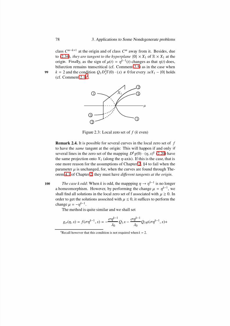
8/2/2019 Rabier-Lectures on Topics in One Parameter Bifurcation Problems
http://slidepdf.com/reader/full/rabier-lectures-on-topics-in-one-parameter-bifurcation-problems 88/238
78 3. Applications to Some Nondegenerate problems
class C m−k + 1 at the origin and of class C m away from it. Besides, due
to (2.34) , they are tangent to the hyperplane 0 ×X 1 of R ×X 1 at theorigin. Finally, as the sign of µ(t ) = ηk −1(t ) changes as that η(t ) does,bifurction remains transcritical (cf. Comment 2.5) as in the case whenk = 2 and the condition Q1 D2
xΓ(0) · ( x) 0 for every x X 1 − 0holds99
(cf. Comment 2.1)4 .
2
2
3
31
1
Figure 2.3: Local zero set of f (k even)
Remark 2.4. It is possible for several curves in the local zero set of f to have the same tangent at the origin: This will happen if and only if several lines in the zero set of the mapping Dk g(0) · (η, x)k (2.20 ) havethe same projection onto X 1 (along the η-axis). If this is the case, that isone more reason for the assumptions of Chapter 2, §4 to fail when theparameter µ is unchanged, for, when the curves are found through The-orem 4.1 of Chapter 2, they must have di ff erent tangents at the origin .
The case k odd : When k is odd, the mappping η →ηk −1 is no longer100
a homeomorphism. However, by performing the change µ = ηk −1 , weshall nd all solutions in the local zero set of f associated with µ ≥0. Inorder to get the solutions associted with µ ≤0, it suffices to perform thechange µ = −ηk −1 .
The method is quite similar and we shall set
gσ (η, x) = f (ση k −1 , x) = −ση k −1
λ0Q1 x−
ση k −1
λ0Q1 (ση k −1, x)+
4Recall however that this condition is not required when k = 2.
8/2/2019 Rabier-Lectures on Topics in One Parameter Bifurcation Problems
http://slidepdf.com/reader/full/rabier-lectures-on-topics-in-one-parameter-bifurcation-problems 89/238
3.2. Application to Problems of Bifurction..... 79
+ Q1Γ(ση k −1 , x + (ση k −1 , x)), (2.35)
where σ = ±1. Arguing as in Proposition 2.1 , we nd that the rstnonzero derivative of the mapping gσ at the origin is of order k with
Dk gσ (0) ·(η, x)k = −σ k !λ0
ηk −1 Q1 x + Q1 Dk xΓ(0) ·( x)k Y 1 , (2.36)
for every ( η, x) R ×X 1. Again, two implict condition for the results of Chapter 2, §4 to be available are
X = Ker ( I −λ0 L) Range ( I −λ0 L)(= X 1 Y 2),
(i.e. the algebraic and geometric multiplicities of the characteristic valueof λ0 coincide) and
Q1 Dk xΓ(0) ·( x)k 0 for every x X 1 − 0.
Again, from §1 the mapping Dk g(0)( η, x)k veries the condition ( R − N . D) or not independently of the choice of X 2 and Y 1 so that we cantake X 1 = Y 1 in the applications. With this choice, we get the simplied 101
expressions
gσ (η, x) = −ση k −1
λ0 x + Q1Γ(ση k −1 , x + (ση k −1 , x)), (2.37) σ
Dk gσ (0) ·(η, x)k = −σ k !ηk
−1
λ0 x + Q1 Dk xΓ(0) ·( x)k X 1 , (2.38) σ
for every ( η, x) R × X 1. Also, none of the curves in the local zero set of gσ has a “vertical” tangent at the origin and each curve in the local zeroset of f is of the from
t →( µ(t ), x(t )),
with µ(t ) = ση k −1(t ) and t →(η(t ), x(t )) is one of the curves in the localzero set of gσ (thus of class C m−k + 1 at the origin and of class C m awayfrom it). Each non-trivial curve in the local zero set of f is then also of class C m−k + 1 at the origin and of class C m away from it (the argument is
the same as when k is even) and it is tangent to the hyperplane 0 ×X 1at the origin. For σ = 1 (respectively - 1), the corresponding curves of
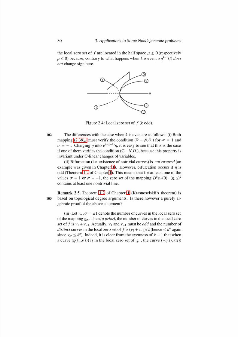
8/2/2019 Rabier-Lectures on Topics in One Parameter Bifurcation Problems
http://slidepdf.com/reader/full/rabier-lectures-on-topics-in-one-parameter-bifurcation-problems 90/238
80 3. Applications to Some Nondegenerate problems
the local zero set of f are located in the half space µ ≥0 (respectively
µ ≤0) because, contrary to what happens when k is even, σηk
−1(t ) does
not change sign here.
2
2
3
31
1
Figure 2.4: Local zero set of f (k odd).
The diff erences with the case when k is even are as follows: (i) Both102
mapping (2.38) σ must verify the condition ( R −N . D.) for σ = 1 andσ = −1. Charging η into eiπ(k −1) η, it is easy to see that this is the caseif one of them veries the condition ( C − N . D.), because this property isinvariant under C -linear changes of variables.
(ii) Bifurcation (i.e. existence of notrivial curves) is not ensured (anexample was given in Chapter 1). However, bifurcation occurs if η isodd (Theorem 1.2 of Chapter 1). This means that for at least one of thevalues σ = 1 or σ = −1, the zero set of the mapping Dk gσ (0) · (η, x)k
contains at least one nontrivial line.
Remark 2.5. Theorem 1.2 of Chapter 1 (Krasnoselskii’s theorem) isbased on topological degree arguments. Is there however a purely al-103
gebraic proof of the above statement?
(iii) Let νσ , σ = ±1 denote the number of curves in the local zero setof the mapping gσ . Then, a priori , the number of curves in the local zeroset of f is ν1 + ν−1 . Actually, ν1 and ν−1 must be odd and the number of distinct curves in the local zero set of f is (ν1 + ν−1)/ 2 (hence ≤k n again
since νσ ≤k n
). Indeed, it is clear from the evenness of k −1 that whena curve ( η(t ), x(t )) is in the local zero set of gσ , the curve ( −η(t ), x(t ))

8/2/2019 Rabier-Lectures on Topics in One Parameter Bifurcation Problems
http://slidepdf.com/reader/full/rabier-lectures-on-topics-in-one-parameter-bifurcation-problems 91/238
3.2. Application to Problems of Bifurction..... 81
is also in it. Both provide the same curve ( µ(t ), x(t )) = (ση k −1 (t ), x(t ))
in th local zero set of f and the two vectors (( d η/ dt )(0)( dx/ dt )(0)) and(−(d η/ dt )(0) , (dx/ dt )(0)) are not collinear if and only if ( dx/ dt )(0) 0,because ( d η/ dt )(0) is 0 as we observed earlier 5 . Now the condition(dx/ dt )(0) 0 is fullled by all the curves in the local zero set of gσ , ex-cept the trivial branch (recall that the correspondence between the curvesin the local zero set of gσ and their tangents at the origin is one-to-one).Hence, each non-trivialcurve in the local zero set of f is provided by twodistinct non-trivial curves in the local zero set of g1 or by two distinctnon-trivial curves in the local zero set of g−1 . Thus, ν1 and ν−1 must beodd and the number of non-trivial curves in the local zero set of f is
ν1
−1
2 +ν
−1
−1
2 =ν1 + ν
−1
2 −1.
Adding the trivial branch, we nd ( ν1 + ν−1)|2 to be the number 104
of distinct curves in the local set of f . Exactly ( ν1 −1)|2 of them aresupercritical (i.e. located in the half-space µ ≥0 of R × X 1) and exactly(ν−1 −1)|2 are subcritical (i.e. located in the half space µ ≤0 of R × X 1).One (the trivial branch) is transcritical . Of course, it may happen thatν1 = 0 or ν−1 = 0 (or both).
Remark 2.6. Recall that in both the case ( k even and k odd ), we madethe a priori assumption X 1 Y 2 (and it turned out that the conditions X 1
∩Y 2 =
0
was necessary). If X 1 Y 2, the trick of changing the
parameter µ into ηk −1 , σ = ±1 does not work: Indeed, the rst nonzeroderivative of g or gσ at the origin remains of order k and its value at thepoint ( η, x) R × X 1 repeated k times reduces to
(η, x) R × X 1 →Q1 Dk xΓ(0) ·( x)k Y 1 .
This mapping never veries the condition (R − N . D.) because of thetrivial branch in its zero set at which its derivative vanishes.
Remark 2.7. We leave it to the reader to check that changing the param-ete µ into a ηk −1 , a 0, when k is even is equivalent to changing it into
5In comment 2.4 and when k is even, but the argument can be repeated when k isodd.
8/2/2019 Rabier-Lectures on Topics in One Parameter Bifurcation Problems
http://slidepdf.com/reader/full/rabier-lectures-on-topics-in-one-parameter-bifurcation-problems 92/238

8/2/2019 Rabier-Lectures on Topics in One Parameter Bifurcation Problems
http://slidepdf.com/reader/full/rabier-lectures-on-topics-in-one-parameter-bifurcation-problems 93/238
3.2. Application to Problems of Bifurction..... 83
This linear form allows us to express the projection operator Q1 onto
the space Y 1. More preciselyQ1 y = y , y y0 ,
for every y X (= Y ). Then, for k even , we nd from ( 2.20 ) that
Dk g(0) ·(η, x)k = −k !ηk −1
λ0 y , x0 + t k y , Dk
xΓ(0) ·( x0)k y0
and proving that this mapping veries the condition ( R − N . D.) amountsto proving that the real-valued mapping of the two real variables η, t given by
(η, t ) R 2
→ −k !ηk −1
λ0 y , x0 + t k y , Dk
xΓ(0)
·( x0 )k R ,
does the same, which is always the case because of the relations y , 107
x0 0 (since X 1 ∩Y 2 = 0) and y , Dk xΓ(0) · ( x0 )k 0 (since
Q1 Dk xΓ(0)|( X 1)k 0). Besides, as expected, the zero set of Dk g(0) ·(η, x)k
is the union of the trivial branch and exactly one nontrivial line , namelythat line for which
t = k ! y , Dk
xΓ(0) ·( x0 )k
λ0 y , x0
1/ k −1
η, η R .
Repeating the arguments we used in the case n ≥2, we see that thecorresponding non-trivial branch in the local ero set of is tangent to the
asis 0 ×X 1 at the origin and located on both sides of it: we are in thepresence of a phenomenon of transcritical bifurcation.
Figure 2.5: Local zero set of f when n = 1, k even ≥4

8/2/2019 Rabier-Lectures on Topics in One Parameter Bifurcation Problems
http://slidepdf.com/reader/full/rabier-lectures-on-topics-in-one-parameter-bifurcation-problems 94/238
84 3. Applications to Some Nondegenerate problems
Analogously, when k is odd, one has (cf. ( (2.38) σ ))
Dk gσ (0) ·(η, x)k = −k !ση k −1t
λ0 y , x0 + t k y , Dk
xΓ(0) ·( x0 )k y0 .
If so, because k −1 is even, the local zero set of this mapping reduces108
to the trivial branch if
sgn y , Dk
xΓ(0) ·( x0 )k
λ0 y , x0= sgn (−σ )
and is the union of the trivial branch and two nontrivial lines, namely,those for which
t = ± k !σ y , Dk
xΓ(0) ·( x0 )k
λ0 y , x0
1/ k −1
η,η R ,
if
sgn y , Dk
xΓ(0) ·( x0)k
λ0 y , x0= sgn σ.
They both provide the same curve in the local zero set of f , locatedon one side of the axis 0 ×X 1 . The bifurcation is either supercriticalor subcritical depending on which among the mappings Dk g1(0) ·(η, x)k
and Dk g−1(0) ·(η, x)k possesses the non-trivial lines in its zero set
Figure 2.6:

8/2/2019 Rabier-Lectures on Topics in One Parameter Bifurcation Problems
http://slidepdf.com/reader/full/rabier-lectures-on-topics-in-one-parameter-bifurcation-problems 95/238
3.3. Application to a Problem...... 85
Remark 2.8. Though the assumptions of this section are stronger than109
those we made in Chapter 1 when n = 1, the regularity of the non-trivialcurve in the local zero set of f is only found to be of class C m−k + 1 at theorigin (but we know it is actually of class C m−1). In contrast, the locationof this curve with respect to the axis 0 × X 1 could not be derived fromthe analysis of Chapter 1 because it clearly depends on the evenness of k , which was ignored in Chapter 1.
Remark 2.9. The assumption ( 2.40 ) can be replaced by
D j xΓ(0)|( X 1 ) j = 0, 0 ≤ j ≤k −1,
Q1 Dk xΓ(0)|( X 1)k 0, (2.41)
or by a suitable combination ( 2.40 ) and (2.41 ) such as in Remark 2.3.
3.3 Application to a Problem with no Branch of Solutions Known a Priori.
We shall here consider the problem of nding the “small” solution ( µ, x) R × X an equation of the form
F ( x) = µ y0 (3.1)
where F is a mapping of class C m, m ≥ 1, in a neighbourhood of theorigin in the Banach space X , with values in another Banch space Y ,such that F (0) = 0 and where y0 is a given element of Y . In order to deal 110
with a situation essentially di ff erent from that of §2 we shall assume
y0 RangeD xF (0). (3.2)
First, we write the problem in the form
G ( µ, x) = 0,
with G ( µ, x) = F ( x) − µ y0 . (3.3)
8/2/2019 Rabier-Lectures on Topics in One Parameter Bifurcation Problems
http://slidepdf.com/reader/full/rabier-lectures-on-topics-in-one-parameter-bifurcation-problems 96/238
86 3. Applications to Some Nondegenerate problems
Due to ( 3.2 ), the space Y 2 = RangeDG (0) is
Y 2 = RangeDG (0) = R y0 RangeD xF (0) (3.4)
whereas, setting X 1 = KerD xF (0),
one has X 1 = KerDG (0) = 0 × X 1. (3.6)
As required in these notes, we shall assume that DG (0) L (R × X , Y )is a Fredholm operator with index 1, which will be for instance, the case,if D xF (0) is a Fredholm operator with index 0. As usual, n will denotethe codimension of the space Y 2.
When n = 0, the same problem has already been encountered inChapter 1. The situation was simple because the Implict function the-orem applied so that the local zero set of G was found to be made up111
of exactly one curve of class C m. Recall that this curve has a “vertical”tangent (i.e. the one - dimensional space 0 ×X 1) at the origin and wementioned that two typical cases where those when the origin is eithera “turning point” or a “hysteresis point” (cf. Fig. 3.2 of Chapter 1). Adetailed explanation of these phenomena will be given later on. For thetime being, we shall assume n ≥1. Performing the Lyapunov-Schmidtreduction as described in Chapter 1, §2 and setting x = ( µ, x), we get areduced equation of the general form
f ( x) = Q1G ( x + ( x)),
where x belongs to some neighbourhood of the origin in the space X 1and Q1 denotes the projection operator onto some given complement of the space Y 2. Because of ( 3.6), the variable x X 1 identies itself withthe variable x X 1 . Provided we choose the complement X 2 of the space X 1 of the form
X 2 = R × X 2 ,
where X 2 is a given topological complement of X 1 , the mapping canbe identied with a pair
( x) = ( µ( x), ( x)) R × X 2,
8/2/2019 Rabier-Lectures on Topics in One Parameter Bifurcation Problems
http://slidepdf.com/reader/full/rabier-lectures-on-topics-in-one-parameter-bifurcation-problems 97/238
3.3. Application to a Problem...... 87
of mappings of class C m aroun the origin.
As Q1 y0
= 0 (cf. (3.4 )), the reduced equation takes the form
f ( x) = Q1F ( x + ( x)) = 0. (3.7)
The results of Chapter 2, §4 will be available if the rst nonzero 112
derivative of the above mapping at the origin veries the condition ( R − N . D.). A general frame work in which it takes a very simple expressionis as follows: Consider the integer 2 ≤k ≤m characteried by
Q1 D j xF (0)|( X 1 ) j = 0, 0 ≤ j ≤k −1,
Q1 Dk xF (0)|( X 1 )k 0,
(3.8)
(if such a k exists of course) and let k 1 and k 1 be dened by
k 1 = min0 ≤ j ≤k , Q1 D j xF (0) 0, (3.9)
k 1 = min0 ≤ j ≤k , D j xF (0)|( X 1 ) j 0, (3.10)
so that 2 ≤k 1 , k 1 ≤k . Under the condition 8
k ≤k 1 + k 1 −2, (3.11)
the rst non-zero derivative of the mapping f in (3.7) at the origin is of order k and its value at the point x X 1 repeated k times is
Dk f (0) ·( x)k = Q1 Dk xF (0) ·( x)k . (3.12)
The reader can easily check this assertion in the two frequently en-counted particular cases k = k 1 or k = k 1, namely when
Q1 D j xF (0) = 0, 0 ≤ j ≤k −1,
or D j
xF (0)|( X 1 ) j = 0, 0 ≤ j ≤k −1.
113
8Observe that none of the integers k , k 1 and k 1 depends on the choice of the spaceY 1.
8/2/2019 Rabier-Lectures on Topics in One Parameter Bifurcation Problems
http://slidepdf.com/reader/full/rabier-lectures-on-topics-in-one-parameter-bifurcation-problems 98/238
88 3. Applications to Some Nondegenerate problems
For a general result, see [ 31]. When ( 3.11 ) holds and the mapping
(3.12 ) veries the condition ( R − N . D.) (a property which is easily seento be independent of the choice of the space Y 1) the largest number of curves in the local zero set of f - hence of G - is k n. Note here that
n = dimX 1 −1(= dimKerD xF (0) −1). (3.13)
Of course, the curves are of class C m−k + 1 at the origin and of classC m away from it.
Remark 3.1. In contrast to the case n = 0, it is quite possible that theorigin is an isolated solution . For instance, let X = Y = R 3 and chooseF as
F ( x1 , x2 , x3) = x21 + x22 + x23
0 x3
while y0 is taken as
y0 =010
.
The only solution of the equation F ( x1 , x2 , x3) = µ y0 is µ = x1 = x2 = x3 = 0. Nevertheless, ( 3.8) is fullled with k = 2 and (3.11 ) holds.The mapping (3.13 ) associated with this example is
( x1 , x2 , x3) R 3→x2
1 + x22 + x2
3 R
and veries the condition ( R − N . D.) trivially.114
Observe, however, that existence of at least one curve of solution isgenerated by comment 1.3 of Chapter 2 when k is odd .
The analysis we have made does not provide any information onthe location of the curves. Incidentally, such information was obtainedin the problem we considered in the previous section after we had tomake a change of parameter to nd the structure of its set of solutions.
Here, one has no such motivation indeed since a satisfactory answer hasalready been given to this question but it is not without interest to see
8/2/2019 Rabier-Lectures on Topics in One Parameter Bifurcation Problems
http://slidepdf.com/reader/full/rabier-lectures-on-topics-in-one-parameter-bifurcation-problems 99/238
3.3. Application to a Problem...... 89
where a change of parameter could lead us: setting µ = η p for some
integer p ≥2, we have to solve the problem
G (η, u) = G (η p, x) = F ( x) −η p y0 = 0. (3.14)
The main di ff erence with the case when the parameter µ is uncha-nged is that (compare with ( 3.4) and (3.6))
Y 2 = RangeD G (0) = RangeD xF (0) , (3.15)
ˆ X 1 = KerD G (0) = R ×KerD xF (0) = R × X 1 . (3.16)
Thus, the mapping DG (0) will be a Fredholm operator with index1 if and only if the mapping D xF (0) is a Fredholm operator with in-dex 0 (namely, Range D xF (0) must be closed). Also, with the previousdenition of n (= codim Y 2), one has
codim Y 2 = n + 1(= n) ≥1, (3.17)
dim Ker ˆ X = n + 2(= n + 1) ≥2. (3.18)
We shall denote by Y 1 any complement of Y 2 and call Q1 and Q2 115
the projection operators onto Y 1 and Y 2 respectively. Performing theLyapunov-Schmidt reduction of the problem ( 3.14 ), we nd a reducedequation of the general form
g( ˆ x) = Q1G ( ˆ x + ˆ ( ˆ x)).
Here, the variable ˆ x of the space ˆ X 1 = R × X 1 is the pair ( η, x) R × X 1and the mapping ψ takes its values in some topological complement ˆ X 2of the space ˆ X 1 . Choosing ˆ X 2 = 0 ×X 2 where X 2 is any topologicalcomplement of X 1, the mapping ψ identies itself with a mapping ψwith values in X 2 so that
g(η, x) = Q1 F ( x + ˆ (η, x)) −η pQ1 y0
(note that Q1 y0 0 since y0 Range D xF (0) by hypothesis). At this
stage, it is necessary for a better understanding to examine how the map-ping ˆ is related to the variable µ through the change µ = η p. To this

8/2/2019 Rabier-Lectures on Topics in One Parameter Bifurcation Problems
http://slidepdf.com/reader/full/rabier-lectures-on-topics-in-one-parameter-bifurcation-problems 100/238
90 3. Applications to Some Nondegenerate problems
end, write each element x X in the form x = x1 + x2 with x1 X 1 and
x2 X 2 . The equation G ( µ, x) = 0 becomes equivalent to the system
Q1G ( µ, x1 + x2) = 0,
Q2G ( µ, x1 + x2) = 0.
As Q2 D xG (0) = Q2 D xF (0) Isom ( X 2 , Y 2), the second equation issolved by the Implict function theorem and is equivalent to
x2 = ˆ ( µ, x1 ),
where ˆ is mapping of class C m around the origin in R × X 1 with values116
in X 2, uniquely determined by the condition ˆ (0) = 0. Referring to therst equation, we nd a reduced equation
f ( µ, x1) = Q1G ( µ, x1 + ˆ ( µ, x1 ))
for ( µ, x1) around the origin in R ×X 1. Dropping the index “1” in thevariable x1 X 1 and using ( 3.3 ), we deduce
ˆ f ( µ, x) = Q1G ( µ, x + ˆ ( µ, x)), (3.19)
for ( µ, x) around the origin of R ×X 1 . Note that this reduction di ff ersfrom the Lyapunov-Schmidt reduction as it was described in Chapter 1because the space Y
2is not the range of the global derivative DG (0) but
only the range of the partial derivative D xG (0). In particular, D ˆ (0) 0since D µ ˆ (0) 0 in general. However, the local zero set of ˆ f (3.19 )immediately provides the local zero set of G and a simple vericationshows that the mapping ψ and ˆ are linked through the relation
ψ(η, x) = ˆ (η p, x).
It follows that
g(η, x) = ˆ f (η p, x) = Q1 F ( x + ˆ (η p, x)) −η pQ1 y0 .
Again, the problem now is to nd the rst non-zero derivative of g at the origin. Of course, it will depend on p but since the condition
8/2/2019 Rabier-Lectures on Topics in One Parameter Bifurcation Problems
http://slidepdf.com/reader/full/rabier-lectures-on-topics-in-one-parameter-bifurcation-problems 101/238
3.3. Application to a Problem...... 91
(R −N . D.) must hold under general hypotheses, it is possible to show
that the only available value of p is p = k where the integer 2 ≤ k ≤m117is characterized by
Q1 D j xF (0)|( X 1 ) j = 0, 0 ≤ j ≤k −1,
Q1 Dk xF (0)|( X 1 )k 0.
(3.20)
The process allowing the selection of p should be described in ageneral framework rather than on this particular example but even so,it remains quite technical and will not be presented here (see [ 31] fordetails).
The mapping ˆg corresponding to the choice p = k is
g(η, x) = ˆ f (ηk , x) = Q1 F ( x + ˆ (ηk , x)) −ηk Q1 y0 . (3.21)
Setting
k 1 = min0 ≤ j ≤k , Q1 D j xF (0) 0, (3.22)
k 1 = min0 ≤ j ≤k , D j xF (0)|( X 1 ) j 0, (3.23)
one has 2 ≤k 1 , k 1 ≤k . Clearly, none of the integers k , k 1 and k 1 dependson the choice of the space Y 1 and, under the condition
k
≤k
1+ k 1
−2, (3.24)the rst non-zero derivative of the mapping ˆ g (3.21 ) at the origin is of order k with
Dk g(0) ·(η, x)k = Q1 Dk xF (0) ·( x)k −k !ηk Q1 y0 Y 1 , (3.25)
for every ( η, x) R ×X 1 . The reader can check there formulae in theparticular cases k 1 = k or k 1 = k , namely 118
Q1 D j xF (0) = 0, 0 ≤ j ≤k −1,
or D j xF (0)|( x1 ) j = 0, 0 ≤ j ≤k −1.

8/2/2019 Rabier-Lectures on Topics in One Parameter Bifurcation Problems
http://slidepdf.com/reader/full/rabier-lectures-on-topics-in-one-parameter-bifurcation-problems 102/238
92 3. Applications to Some Nondegenerate problems
In the general case, see [ 31]. If the mapping ( 2.25 ) veries the con-
dition ( R − N . D.) and k is odd, the local zero set of ˆ g provides that of ˆ f (3.19 ) immediately. If k is even the local zero set of ˆg gives the elementsof the local zero set of ˆ f associated with µ ≥0. So as to get the elementsassociated with µ ≤0, the change µ = −ηk is necessary too. When k iseven , we must then examine both the mappings
gσ (η, x) = ˆ f (ση k , x) = Q1 Dk xF (0) ·( x)k −k !ση k Q1 y0 Y 1 , (3.26) σ
where σ = ±1 and we have
Dk gσ (0) ·(η, x)k = Q1 Dk xF (0) ·( x)k
−k !ση k Q1 y0 , ((3.27) σ )
for (η, x) R × X 1.Assume rst that k is odd and the mapping ( 3.25 ) veries the con-
dition ( R −N . D.). Arguing as in §1, we see that its zero set containsno “vertical” line (i.e. no line contained in the hyperplane 0 ×X 1).Therefore, if t →(η(t ), x(t )) is one of the curves in the local zero set of g, one has
d ηdt
(0) 0,
so that the curve is located on both sides of the hyperplane 0 ×X 1 in119R × X 1 .
2
2
1
1
Figure 3.1: Local zero set of ˆ g (k odd).
Asˆk is odd and the mapping n →η
k
is a homeomorphism of R , thecorresponding curve ( µ(t ), x(t )) with µ(t ) = ηk (t ) in the local zero set of
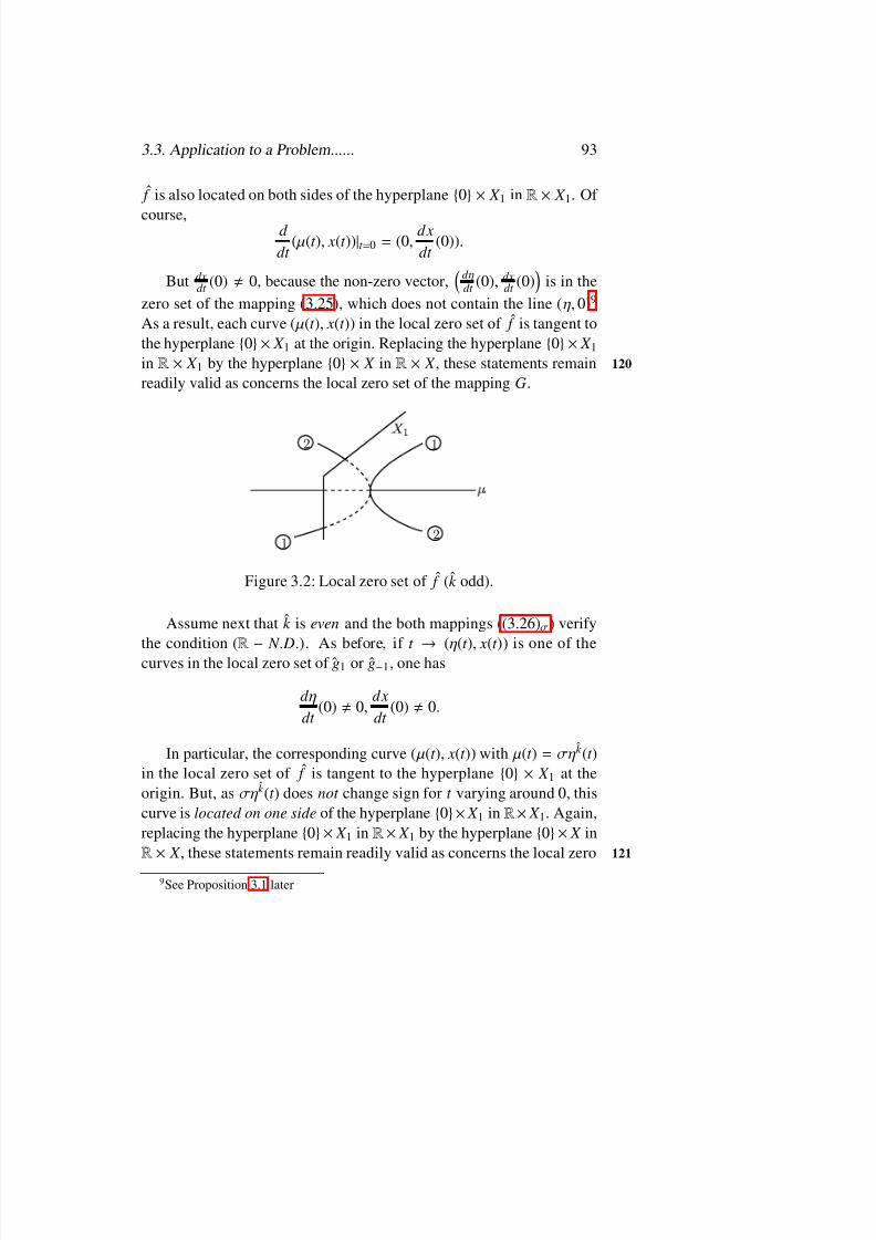
8/2/2019 Rabier-Lectures on Topics in One Parameter Bifurcation Problems
http://slidepdf.com/reader/full/rabier-lectures-on-topics-in-one-parameter-bifurcation-problems 103/238
3.3. Application to a Problem...... 93
ˆ f is also located on both sides of the hyperplane 0 ×X 1 in R ×X 1. Of
course, d dt
( µ(t ), x(t ))|t = 0 = (0,dxdt
(0)) .
But dxdt (0) 0, because the non-zero vector, d η
dt (0) , dxdt (0) is in the
zero set of the mapping ( 3.25 ), which does not contain the line ( η, 0)9
As a result, each curve ( µ(t ), x(t )) in the local zero set of ˆ f is tangent tothe hyperplane 0× X 1 at the origin. Replacing the hyperplane 0× X 1in R ×X 1 by the hyperplane 0 ×X in R ×X , these statements remain 120
readily valid as concerns the local zero set of the mapping G .
2
21
1
Figure 3.2: Local zero set of ˆ f (k odd).
Assume next that k is even and the both mappings ( (3.26) σ ) verifythe condition ( R
−N . D.). As before, if t
→(η(t ), x(t )) is one of the
curves in the local zero set of ˆ g1 or g−1 , one has
d ηdt
(0) 0,dxdt
(0) 0.
In particular, the corresponding curve ( µ(t ), x(t )) with µ(t ) = ση k (t )in the local zero set of ˆ f is tangent to the hyperplane 0 ×X 1 at theorigin. But, as ση k (t ) does not change sign for t varying around 0, thiscurve is located on one side of the hyperplane 0× X 1 in R × X 1. Again,replacing the hyperplane 0× X 1 in R × X 1 by the hyperplane 0× X inR
×X , these statements remain readily valid as concerns the local zero 121
9See Proposition 3.1 later

8/2/2019 Rabier-Lectures on Topics in One Parameter Bifurcation Problems
http://slidepdf.com/reader/full/rabier-lectures-on-topics-in-one-parameter-bifurcation-problems 104/238
94 3. Applications to Some Nondegenerate problems
set of the mapping G .
Figure 3.3: Local zero set of ˆ f (k even)
We are now going to relate the assumptions we make for solving theproblem after changing the parameter µ into ηk or ση k to the assump-tions we made earlier to solve it without changing µ. First, observe thatthe integer k characterized by (3.18 ). Indeed, k is independent of thechoice of the space Y 1 and from the denitions, it is immediate that Y 1can be chosen so that
Y 1 Y 1 (3.28)
where Y 1 is any space chosen for dening k . By the same arguments,note that122
k 1
≤k 1 , k 1
≤k 1 , (3.29)
(cf. ( 3.9 )-(3.10 ) and (3.22 )-(3.23 )). But we shall see that the integersk and k must coincide for the mappings ( 3.25 ) or (3.27) σ to verify thecondition ( R − N . D.) when n ≥1. This is proved in
Proposition 3.1. Assume k is odd (resp. even). Then, the mapping(3.25 ) (resp. (3.27)1 and (3.27)−1 ) eries the condition (R −N . D.) isand only if
Q1 Dk xF (0) ·( x)k 0, (3.30)
for every x X 1 − 0and the mapping
x X 1 →Q1 Dk xF (0) ·( x)k Y 1 , (3.31)
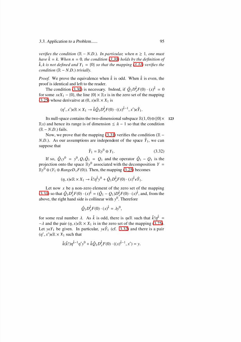
8/2/2019 Rabier-Lectures on Topics in One Parameter Bifurcation Problems
http://slidepdf.com/reader/full/rabier-lectures-on-topics-in-one-parameter-bifurcation-problems 105/238
3.3. Application to a Problem...... 95
veries the condition (R −N . D.). In particular, when n ≥1 , one must
have k = k. When n = 0 , the condition ( 3.30) holds by the denition of k , k is not dened and Y 1 = 0so that the mapping ( 3.31 ) veries thecondition (R − N . D.) trivially.
Proof. We prove the equivalence when k is odd. When k is even, theproof is identical and left to the reader.
The condition ( 3.30 ) is necessary. Indeed, if Q1 Dk xF (0) · ( x)k = 0
for some x X 1 − 0, the line 0 ×R x is in the zero set of the mapping(3.25 ) whose derivaitve at (0 , x) R × X 1 is
(η′, x′) R × X 1 →k Q1 Dk xF (0) ·(( x)k −1 , x′) Y 1 .
Its null-space contains the two-dimensional subspace R (1, 0) (0× 123R x) and hence its range is of dimension ≤ n −1 so that the condition(R − N . D.) fails.
Now, we prove that the mapping ( 3.31 ) veries the condition ( R − N . D.). As our assumptions are independent of the space Y 1, we cansuppose that
Y 1 = R y0 Y 1 . (3.32)
If so, Q1 y0 = y0 , Q1 Q1 = Q1 and the operator Q1 −Q1 is theprojection onto the space R y0 associated with the decomposition Y =R y0 (Y 1 RangeD xF (0)). Then, the mapping ( 3.25) becomes
(η, x) R × X 1 →k !ηk y
0+ Q1 D
k xF (0) ·( x)
k Y 1.
Let now x be a non-zero element of the zero set of the mapping(3.31 ) so that Q1 Dk
xF (0) ·( x)k = (Q1 −Q1 ) Dk xF (0) ·( x)k , and, from the
above, the right hand side is collinear with y0 . Therefore
Q1 Dk xF (0) ·( x)k = λ y0 ,
for some real number λ. As k is odd, there is η R such that k !ηk =
−λ and the pair ( η, x) R ×X 1 is in the zero set of the mapping ( 3.25 ).Let y Y 1 be given. In particular, y Y 1 (cf. 3.32 ) and there is a pair(η′, x′) R
× X 1 such that
k (k !)ηk −1η′ y0 + k Q1 Dk xF (0) ·(( x)k −1, x′) = y.
8/2/2019 Rabier-Lectures on Topics in One Parameter Bifurcation Problems
http://slidepdf.com/reader/full/rabier-lectures-on-topics-in-one-parameter-bifurcation-problems 106/238
8/2/2019 Rabier-Lectures on Topics in One Parameter Bifurcation Problems
http://slidepdf.com/reader/full/rabier-lectures-on-topics-in-one-parameter-bifurcation-problems 107/238
3.3. Application to a Problem...... 97
c) Q1 Dk xF (0) ·( x)k 0 for every x X 1 − 0,
d) the mapping x X 1 →Q1 Dk
xF (0) ·( x)k Y 1 ,
veries the condition ( R − N . D.).
In any case, these assumptions are stronger than those made whenthe local zero set of G is determined without chaging the parameter µ(see in particular ( 3.29 ) and recall that k must equal k when n ≥1) andthe conclusions are not as precise : The number of curves is found to be
≤k n = k n+ 1 . When n ≥1, this upper bound is nothing but k n+ 1 (but weknow that it is actually k n) and k when n = 0 (but we know that there
is exactly one curve). The regularity we obtain is of class C m
−k + 1
atthe origin and of class C m away from it, which agress with the previousresult if n ≥1 (since k = k ) but is not as good when n = 0 (the curve isactually of class C m at the origin). However, the additional informationwhich may be of interest is the location of the curves in the space R × X .In particular, when n = 0, the reader can immediately deduce, from the 126
appropriate discussion given before, that the origin is a “turning point”when k is even and a “hysteresis point” when k is odd . When n ≥ 1,bifurcation may occur but the origin can be an isolated solutoion as well(see the example given in Remark 3.1 ).

8/2/2019 Rabier-Lectures on Topics in One Parameter Bifurcation Problems
http://slidepdf.com/reader/full/rabier-lectures-on-topics-in-one-parameter-bifurcation-problems 108/238

8/2/2019 Rabier-Lectures on Topics in One Parameter Bifurcation Problems
http://slidepdf.com/reader/full/rabier-lectures-on-topics-in-one-parameter-bifurcation-problems 109/238
Chapter 4
An Algorithm for the
Computation of the Branches
IN THIS CHAPTER, we describe an algorithm for nding the local zero 127
set of a mapping f verifying the assumptions of Chapter 2. When f isexplicitly known , we obtain an iterative scheme with optimal rate of con-vergence. However, in the applications to one paramenter problems inBanach spaces (such as those described in Chapter 3 for instance) f is the reduced mapping which is known only theoretically , because themapping coming from the Lyapunov-Schmidt reduction (cf. Chap-ter 1, §2) involved in the denition of f is found through the implict function theorem .
What is explicitly available in this case is only a sequence ( f ℓ ) of mappings tending to f in some appropriate way and the algorithm mustbe modied accordingly. Again, optimal rate of convergence can beestablished but the proof is more delicate. For the sake of brevity, weshall only outline the technical di ff erences which occur. The expositionfollows Rabier-E1-Hajji [ 33]. Full details can be found in Appendix 2.This chapter is completed by an explicit description of the algorithm inthe case of problems of bifurcation from the trivial branch. A compar-
ison with the classical “Lyapunov-Schmidt method” is given as a con-clusion.
99
8/2/2019 Rabier-Lectures on Topics in One Parameter Bifurcation Problems
http://slidepdf.com/reader/full/rabier-lectures-on-topics-in-one-parameter-bifurcation-problems 110/238
100 4. An Algorithm for the Computation of the Branches
4.1 A Short Review of the Method of Chapter II.
In Chapter 2, we considered the problem of nding the local zero set128
of a mapping f of class C m, m ≥ 1, from R n+ 1 into R n (recall that itis not restrictive to assume that f is dened everywhere) satisfying thefollowing condition: There is an integer 1 ≤k ≤m such that
D j f (0) = 0 0 ≤ j ≤k −1,
and the mapping
ξ R n+ 1→q( ξ ) = Dk f (0) ·( ξ )k R n ,
veries the condition ( R − N . D.). Under this assumption, the set
ξ S n ; q( ξ ) = 0is nite and consists of the 2 ν elements ξ j0, 1 ≤ j ≤2ν. Of course, asthe origin is an isolated solutioon of the equation f ( x) = 0 when ν = 0,it is not restrictive to limit ourselves to the case ν ≥1 for dening thealgorithm. This assumption will be implicitly made through-out thischapter.
Setting, for ( t , ξ ) R ×R n+ 1
g(t , ξ ) =k !t k f (t ξ ) if t 0,
g(0, ξ ) = q( ξ ),it was observed for r > 0 that nding the solution x of the equation f ( x) = 0 with 0 < || x||= t < r was equivalent to nding x of the form129
x = t ξ where
0 < |t | < r , ξ S n ,
g(t , ξ ) = 0.
Next, an essential step consisted in proving for r > 0 small enoughthat the above equation was equivalent to solving the problem
0 < |t |< r , ξ
2ν
j= 1σ j,

8/2/2019 Rabier-Lectures on Topics in One Parameter Bifurcation Problems
http://slidepdf.com/reader/full/rabier-lectures-on-topics-in-one-parameter-bifurcation-problems 111/238
4.2. Equivalence of Each Equation with a... 101
g(t , ξ ) = 0,
where, for each 1 ≤ j ≤2ν, σ j denotes an arbitrary neighbourhood of ξ j0 in S n . Taking the σ j’s disjoint, the problem reduces to the study of 2ν independent equations
0 < |t |< r , ξ σ j,
g(t , ξ ) = 0,
for 1
≤j
≤2ν where actually, ν of them (properly selected) are suf-
cient, to provide all the other ν solutions because of symmetry prop-erties. From a practical point of view, it remains to solve the equationg(t , ξ ) = 0 for |t | small enough and ξ S n around one of the points ξ j0 .
4.2 Equivalence of Each Equation with a FixedPoint Problem.
Since the specic value of the index j is not important, we shall denoteany one of the points ξ j0 by ξ 0 . Given δ > 0, we call the closed ball 130
in R n+ 1 with centre ξ 0 and radius δ/ 2. The diameter δ of the ball isalways suppposed to satisfy the condition
0 < δ < 1. (2.1)
Finally, we denote by C the spherical cap centered at ξ 0 (playing therole of the negihbourhood σ j) dened by
C = ∩S n (2.2)
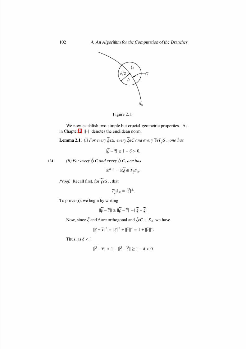
8/2/2019 Rabier-Lectures on Topics in One Parameter Bifurcation Problems
http://slidepdf.com/reader/full/rabier-lectures-on-topics-in-one-parameter-bifurcation-problems 112/238
102 4. An Algorithm for the Computation of the Branches
Figure 2.1:
We now establish two simple but crucial geometric properties. Asin Chapter 2, | |· | |denotes the euclidean norm.
Lemma 2.1. (i) For every ξ , every ζ C and every τ T ζ S n , one has
| ξ −τ | ≥1 −δ > 0.
(ii) For every ξ C and every ζ C, one has131
R n+ 1 = R ξ T ζ S n .
Proof. Recall rst, for ζ S n , thatT ζ S n = ζ .
To prove (i), we begin by writing
|| ξ −τ || ≥ ||ζ −τ | |−|| ξ −ζ ||Now, since ζ and τ are orthogonal and ζ C S n , we have
||ζ −τ ||2 = ||ζ ||2 + ||τ ||2 = 1 + ||τ ||2 .
Thus, as δ < 1
|| ξ −τ ||> 1 − || ξ −ζ || ≥1 −δ > 0.

8/2/2019 Rabier-Lectures on Topics in One Parameter Bifurcation Problems
http://slidepdf.com/reader/full/rabier-lectures-on-topics-in-one-parameter-bifurcation-problems 113/238
4.2. Equivalence of Each Equation with a... 103
Next, to prove (ii), it su ffices to show that R ξ ∩T ζ S n = 0, namely
that ξ T ζ S n = ζ . But a simple calulation shows that ξ C and ζ C are never orthogonal where
δ < 2 2 −√ 2and hence when δ < 1.
Since the mapping q satises the condition ( R − N . D.) and ξ 0 is oneof the points ξ j0 , we know that
Dq( ξ 0)|T ξ 0S n I som (T ξ 0 S n , R n).
Lemma 2.2. After shrinking δ > 0 if necessary, one has
Dq( ξ )|T ξ S n I som (T ξ S n , R n),
for every ξ C. Besides, setting 132
A( ξ ) = ( Dq( ξ )|T ξ S n )−1 L (R n , T ξ S n) L (R n , R n+ 1 ), (2.3)
one has A C 0(C , L (R n , R n+ 1 )).
Proof. Let B1 be the open unit ball in R n
B1 = ξ ′ R n ; || ξ ′||< 1.By identifying R n+ 1 with the product R n ×R ξ 0, the spherical cap C
is homeomorphic to the closed ball Bd / 2 R n centred at the origin withdiameter
d = δ 1 −δ2
16
12
< 1.
This homeomorophism is induced by a C ∞-mapping
ξ ′ B1 →θ ( ξ ′) = ( ξ ′, (1 − || ξ ′||2 )
12 ξ 0) R n+ 1

8/2/2019 Rabier-Lectures on Topics in One Parameter Bifurcation Problems
http://slidepdf.com/reader/full/rabier-lectures-on-topics-in-one-parameter-bifurcation-problems 114/238
104 4. An Algorithm for the Computation of the Branches
It is immediately checked that
Dθ ( ξ ′) I som(R n , T θ ( ξ ′)S n ) L (R n , R n+ 1), (2.4)
for every ξ ′ B1 .The mapping q • θ is of class C ∞from B1 into R n and by di ff erenti-
ating D(q • θ )( ξ ′) = Dq (θ ( ξ ′)) · Dθ ( ξ ′).
Since the mapping Dθ ( ξ ′) takes its values in the space T θ ( ξ ′)S n , this133
can be rewritten as
D(q • θ )( ξ ′) = Dq (θ ( ξ ′))|T θ ( ξ ′)S n · Dθ ( ξ ′). (2.5)
In particular, for ξ ′ = 0 D(q • θ )(0) = Dq ( ξ 0)|T ξ 0
S n · Dθ (0) .
As Dq ( ξ 0)|T ξ 0S n I som (T ξ 0 S n , R n) and Dθ (0) I som (R n , T ξ 0 S n), we
deduce D(q • θ )(0) I som (R )n .
By continuity, we may assume that d > 0 (or, equivalently, δ > 0)has been chosen small enough for D(q •θ )( ξ ′) to be an isomorphism forevery ξ ′ Bd / 2 . Together with ( 2.4 ), relation ( 2.5 ) shows that
Dq(θ ( ξ ′))|T θ ( ξ
′)S
n
= D(q
•θ )( ξ ′)
·[ Dθ ( ξ ′)]−1 I som (T θ ( ξ
′)S n , R n). (2.6)
Hence Dq( ξ )|T ξ S n I som (T ξ S n , R n),
for every ξ C since θ is a bijection from Bd / 2 to C . Now, taking theinverse in ( 2.6 ) and according to the denition of A in (2.3) , we get
A(θ ( ξ ′)) = [ Dq(θ ( ξ ′))|T θ ( ξ ′)S n ]−1 = Dθ ( ξ ′) ·( D(q • θ )( ξ ′))−1 .
The continuity of the mappings Dθ (with values in L (R n , R n+ 1)) and D(q • θ ) (with values in Isom ( R n)) and the continuity of the mapping134
L →L−1 in teh set Isom ( R n) shows that the mapping A•θ is continuous
on the ball Bd / 2 . The continuity of A follows since θ is a homeomorphisnbetween Bd / 2 and C .

8/2/2019 Rabier-Lectures on Topics in One Parameter Bifurcation Problems
http://slidepdf.com/reader/full/rabier-lectures-on-topics-in-one-parameter-bifurcation-problems 115/238
4.2. Equivalence of Each Equation with a... 105
Remark 2.1. With an obvious modication of the above arguments, we
see that the mapping A • θ is actually C ∞around the origin of Rn. As
θ −1 is a chart of the sphere S n centered at the point ξ 0, this means that A is of class C ∞ on a neighbourhood of ξ 0 in the sphere S n . Moregenerally, replacing the mapping q( ξ ) by q(t , ξ ) a similar proof showsthat the mapping
(t , ξ ) →[ D ξ g(t , ξ )|T ξ S n ]−1
is of class C ℓ in a neighbourhood of (0 , ξ 0) in R ×S n whenever D ξ g is of class C ℓ . This result was used in the proof of Theorem 4.1 of Chapter 2(with ℓ = m −k ).
Let us now x 0 < δ < 1 such that Lemma 2.2 holds. Given a triple(t , ζ 0, ξ ) R ×C × , the mapping
M (t , ζ 0, ξ ) = ξ − A(ζ 0) ·g(t , ξ ) R n+ 1 , (2.7)
is well-dened ane we have (recalling that g(0, ξ 0) = q( ξ 0 ) = 0)
M (0, ζ 0 , ξ 0) = ξ 0 . (2.8)
Taking ζ = ζ 0 and τ = A(ζ 0) ·g(t , ξ ) in Lemma 2.1(i), we get
|| M (t , ζ 0 , ξ )|| ≥1 −δ > 0.
Thus, the mapping 135
N (t , ζ 0 , ξ ) =M (t , ζ 0, ξ )
|| M (t , ζ 0 , ξ )|| S n , (2.9)
is well-dened in R ×C × and
N (0, ζ 0 , ξ 0) = ξ 0 . (2.10)
Theorem 2.1. Let (t , ζ 0 ) R ×C be given.
(i) Let ξ C be such that g (t , ξ ) = 0. Then ξ is a xed point of themapping N (t , ζ 0 , ·)

8/2/2019 Rabier-Lectures on Topics in One Parameter Bifurcation Problems
http://slidepdf.com/reader/full/rabier-lectures-on-topics-in-one-parameter-bifurcation-problems 116/238
106 4. An Algorithm for the Computation of the Branches
(ii) Conversely, let ξ be a xed point of the mapping N (t , ζ 0 , ·).Then, ξ C and g (t , ξ ) = 0.
Proof. Part (i) is obvious since, for ξ C such that g(t , ξ ) = 0 one has N (t , ζ 0 , ξ ) = ξ/ || ξ || = ξ . Conversely, the mapping N (t , ζ 0 , ·) takes itsvalues in S n so that any xed point ξ of the mapping N (t , ζ 0 , ·) mustbelong to ∩S n = C . Next, the relation N (t , ζ 0 , ξ ) = ξ also becomes
ξ (1 − || ξ − A(ζ 0) ·g(t , ξ )||) = A( ξ 0 ) ·g(t , ξ ).
But the left hand side is collinear with ξ , while the right hand sidebelongs to the space T ζ 0 S n. By lemma 2.1(ii), both sides must vanish.
In prticular, A(ζ 0)
·g(t , ξ ) = 0 and hence g(t , ξ ) = 0 since the linear
operator A(ζ 0) is one-to-one.
Remark 2.2. As announced, the problem reduces to nding the xedpoints of a given mapping. We emphasize that it is essential, in practice,that the vector ζ 0 be allowed to be arbitrary in C . Indeed, the “natural”136
choice ζ 0 = ξ 0 is not realistic in the applications beacuse ξ 0 is not knownexactly in general.
4.3 Convergence of the Successive ApproximationMethod.
From Theorem 2.1, a constructive method for nding the solutions of the equation g(t , ξ ) = 0 in R ×C consists in applying the successiveapproximation method to the mapping
ξ →N (t , ζ 0 , ξ ) C , (3.1)
where ζ 0 C is arbitrarily xed. In what follows, we prove after shrink-ing δ if necessary that there is r > 0 such that the mapping (3.1 ) is acontraction of into itself for every pair ( t , ζ ) (−r , r ) ×C .
As a preliminary step, let us observe, by the continuity of the map-
ping A (Lemma 2.2) and by the continuity of g and D ξ g on R ×Rn+ 1
(cf.Chapter 2, Lemma 3.3) , that the mapping M is continuous on R ×C ×
8/2/2019 Rabier-Lectures on Topics in One Parameter Bifurcation Problems
http://slidepdf.com/reader/full/rabier-lectures-on-topics-in-one-parameter-bifurcation-problems 117/238
4.3. Convergence of the Successive Approximation Method. 107
and its partial derivative D ξ M exists and is continuous on R ×C × .
More precisely, for every h R n+ 1 ,
D ξ M (t , ζ 0, ξ ) ·h = h − A(ζ 0 ) · D ξ g(t , ξ ) ·h.
In particular, with ( t , ζ 0 , ξ ) = (0, ξ 0 , ξ 0) we nd:
D ξ M (t , ξ 0, ξ 0) ·h = h − A( ξ 0) · D ξ g(0, ξ 0) ·h. (3.2)
But D ξ g(0, ξ 0) = Dg ( ξ 0) and by denition of A, it follows that
D ξ M (0, ξ 0, ξ 0)|T ξ 0S n = 0.
137
Next, taking h = ξ 0 in (3.2 ) we nd D ξ M (0, ξ 0 ; ξ 0) · ξ 0 = ξ 0 − A( ξ 0) · D ξ q(0, ξ 0) · ξ 0 = ξ 0,
because D ξ q(0, ξ 0 ) = kq( ξ 0 ) = 0. The space R n+ 1 being the orthogonal
direct sum of the spaces R ξ 0 and T ξ 0 S n , these relations mean that the
partial dericative D ξ M (0, ξ 0, ξ 0) is nothing but the orthogonal projection
onto the space R ξ 0, namely
D ξ M (0, ξ 0, ξ 0) ·h = ( ξ 0|h) ξ 0 ,
for every h R n+ 1 where ( ·|·) denotes the canonical inner product of R n+ 1 .
As a result, the mapping N is continuous on R ×C × and its partialderivative D ξ N exists and is continuous on R ×C × . We now proceedto show that
D ξ N (0, ξ 0 , ξ 0) = 0.
An elementary computation provides
D ξ N (t , ζ 0 , ξ ) ·h = D ξ M (t , ζ 0 , ξ ) ·h
|| M (t , ζ 0 , ξ )|| −( D ξ M (t , ζ 0 , ξ ) ·h| M (t , ζ 0 , ξ ))
|| M (t , ζ 0 , ξ )||3 M (t , ζ 0 , ξ ).
With ( t , ζ 0 , ξ ) = (0, ξ 0 , ξ 0) and since M (0, ξ 0, ξ 0) = ξ 0 and D ξ M (0,
ξ 0 , ξ 0) ·h = ( ξ 0|h), we get
D ξ N (t , ζ 0 , ξ ) ·h = ( ξ 0|h) ξ 0 −(( ξ 0|h) ξ 0| ξ 0) = 0.

8/2/2019 Rabier-Lectures on Topics in One Parameter Bifurcation Problems
http://slidepdf.com/reader/full/rabier-lectures-on-topics-in-one-parameter-bifurcation-problems 118/238
108 4. An Algorithm for the Computation of the Branches
Theorem 3.1. Let 0 < γ < 1 be a given constant. After shrinking 138
δ > 0 if necessary, there exists r > 0 such that the mapping N (t , ζ, ·) is Lipschitz-continuous with constant γ from the ball into itself for every pair (t , ζ ) [−r , r ] ×C.
Proof. From the relation D ξ N (0, ξ 0 , ξ 0) = 0 and the continuity of D ξ N
in R ×C × , we deduce that there is a neighbourhood of (0 , ξ 0 , ξ 0)in R ×S n ×R n+ 1 in which || D ξ N (t , ζ 0 , ξ )|| is bounded by γ . Clearly,after shrinking δ (hence and C simultaneously), the neighbourhoodin question can be taken as the product [ −r , r ] ×C × for r > 0 smallenough. Hence, by Taylor’s formula (since is convex)
|| N (t , ζ 0 , ξ ) − N (t , ζ 0 , ζ )||< γ || ξ −ζ ||for every ( t , ζ 0) [−r , r ] ×C and every ξ, ζ . In other words, for every(t , ζ 0) [−r , r ] ×C , the mapping N (t , ζ, ·) is Lipschitz-continuous withconstant γ in the ball . The property is obviously not a ff ected by arbi-trarily shrinking r > 0. Let us then x δ as above, which determines theball and the spherical cap C . We shall complete the proof by show-ing, for r > 0 small enough, that the mapping N (t , ξ 0 , ·) maps the ballinto itself for every point ( t , ζ 0) [−r , r ] ×C . Indeed, for ξ and since N (0, ζ 0 , ξ 0) = ξ 0 for every ζ 0 C (cf. ( 2.10) ), one has
|| N (t , ζ 0 , ξ ) − ξ 0||= || N (t , ζ 0 , ξ ) − N (0, ζ 0 , ξ 0)|| ≤≤ || N (t , ζ 0 , ξ ) − N (t , ζ 0 , ξ 0)||+ || N (t , ζ 0 , ξ 0) − N (0, ζ 0 , ξ 0)||.The rst term is bounded by γ || ξ − ξ 0||, thus by γδ/ 2. Finally, due139
to the uniform continuity of the function N (·, ·, ξ 0) on compact sets, wededuce that r > 0 can be chosen so that the second term is bounded by(1 −γ )δ/ 2 and our assertion follows.
4.4 Description of the Algorithm.
The algorithm of computation of the solutions of the equation g(t , ξ ) =0 in [−r , r ] ×C is immediate from Theorem 3.1 : xing t [−r , r ] and
8/2/2019 Rabier-Lectures on Topics in One Parameter Bifurcation Problems
http://slidepdf.com/reader/full/rabier-lectures-on-topics-in-one-parameter-bifurcation-problems 119/238
4.4. Description of the Algorithm. 109
choosing an arbitrary element ξ 0 C , we dene the sequence ( ζ ℓ ) through
the formulaζ ℓ + 1 = N (t , ζ 0 , ζ ℓ ), ℓ ≥0. (4.1)
This sequence tends to the unique xed point ξ of the mapping N (t , ζ 0 , ·) which actually belongs to C and is a solution of the equationg(t , ξ ) = 0 (Theorem 2.1).
For t 0, the sequence
xℓ = t ζ ℓ
tends to x = t ξ , one among the 2 ν solutions with euclidean norm |t | of the equation f ( x) = 0. Of course, for t = 0, the sequence ( ζ ℓ ) tends to ξ 0 , unique solution in C of the equation g(0, ξ )(= q( ξ )) = 0.
Remark 4.1. Incidentally, observe that the above algorithm allows tond arbitrarily close approximations of ξ 0 when only a “rough” estimate(i. e. ζ 0 ) of it is known.
Since our algorithm uses nothing but the contraction mapping prin- 140
ciple, the rate of convergence is geometrical . More precisely
||ζ ℓ − ξ ||< γ ℓ ||ζ 0 − ξ ||,
for every ℓ ≥0, where 0 < γ < 1 is the constant involved in Theorem3.1. Thus as the points ζ 0 and ξ belong to the ball , one has ||ζ 0 − ξ ||<δ < 1 and hence
||ζ ℓ − ξ || ≤γ ℓ δ ≤γ ℓ ,
for ℓ > 0. Multiplying these inequalities by |t |, we get
|| xℓ − x|| ≤γ ℓ || x0 − x|| ≤ |t |γ ℓ , (4.2)
for ℓ ≥0.Let us now make the scheme ( 4.1 ) explicit. As
g(t , ξ ) = k !t k f (t ξ ) for t 0,

8/2/2019 Rabier-Lectures on Topics in One Parameter Bifurcation Problems
http://slidepdf.com/reader/full/rabier-lectures-on-topics-in-one-parameter-bifurcation-problems 120/238
110 4. An Algorithm for the Computation of the Branches
and by the denition of the mapping N in (2.9), we get
ζ ℓ + 1 = ζ ℓ
||ζ ℓ ||,
ζ ℓ = ζ ℓ −k !t k A(ζ 0 ) · f (t ζ ℓ ), ℓ ≥0.
(4.3)
A scheme for the computation of the sequence ( xℓ ) can be immedi-ately derived. Since x0 = t ζ , the iterate xℓ + 1 = t ζ ℓ + 1 is dened by
xℓ + 1 = |t | xℓ
|| xℓ ||,
xℓ = xℓ − k !t k −1 A(ζ 0) · f ( xℓ ), ℓ ≥0.
(4.4)
Remark 4.2. When t = 0, the sequence ( ζ ℓ ) is dened by141
ζ ℓ + 1 = ζ ℓ
||ζ ℓ ||,
ζ ℓ = ζ ℓ − A(ζ 0 ) ·q(ζ ℓ ), ℓ ≥0.
Of course, the sequence ( xℓ ) is the constant one xℓ = 0.
Remark 4.3. (Practical method): Note that the computation of the term
A(ζ 0 ) · f ( xℓ ),
does not require the explicit form of the linear operator A(ζ 0). Indeed,by means of classical algorithm for solving linear systems, it is obtainedas the solution τ T ζ 0 S n = ζ 0 of the equation
Dq(ζ 0 ) ·τ = f ( xℓ ). (4.5)
From the fact that the components of the mapping q are polynomi-als and hence are completely determined by a nite number of coe ffi-cients (depending on the derivative Dk f (0)), the linear mapping Dq (ζ 0 )is completely determined by ζ 0 and these coe fficients. The tangent spaceT
ζ S
n=
ζ
0also is completely determined by ζ
0, which makes it pos-
sible to solve the equation (4.5 ) in practice.

8/2/2019 Rabier-Lectures on Topics in One Parameter Bifurcation Problems
http://slidepdf.com/reader/full/rabier-lectures-on-topics-in-one-parameter-bifurcation-problems 121/238
4.5. A Generalization to the Case..... 111
Remark 4.4. The case k = 1 is the case when the Implicit function theo-
rem applies. The mapping q is the linear mapping D f (0) and the vector ξ 0 is a normalized vector of the one-dimensional space Ker D f (0). The142
sequence ( xℓ ) is dened by the simples relation (after choosing x0 = t ζ 0)
xℓ + 1 = |t | xℓ
|| xℓ ||,
xℓ = xℓ −( D f (0)|ζ 0 )−1 f ( xℓ ), ℓ ≥0,
where ζ 0 S n is “close enough” to ξ 0 . This sequence tends to one of the(two) solutions with eucliden norm |t |of the equation f ( x) = 0.
4.5 A Generalization to the Case When the Map-ping f is not Explicitly Known.
For the reasons we explained at the beginning of this chapter, it is im-portant to extend the algorithm described in §4 to the case when themapping f is not explicitly known but a sequence ( f ℓ ) tending to f isavailable.
More precisely, the mapping f verifying the same assumptions asbefore, we shall assume that there is an open neighbourhood O of theorigin in R n+ 1 such that f is the limit of ( f ℓ ) in the space C k (O , R n)(equipped with its usual Banach space structure). Besides, we shall as-sume
D j f ℓ (0) = 0, 0 ≤ j ≤k −1, (5.1)
Dk f ℓ (0) = Dk f (0) , (5.2)
so that the rst k derivatives of f and f ℓ at the origin coincide for everyℓ ≥0.
Remark 5.1. The conditions ( 5.1) -(5.2 ) may seem very restrictive. 143
However, they are quite adapted to the applications to one-parameterproblems in Banch spaces, as we shall see later on.
If this is the case, the mapping
ξ R n+ 1→q( ξ ) = Dk f (0) ·( ξ )k R n , (5.3)

8/2/2019 Rabier-Lectures on Topics in One Parameter Bifurcation Problems
http://slidepdf.com/reader/full/rabier-lectures-on-topics-in-one-parameter-bifurcation-problems 122/238
112 4. An Algorithm for the Computation of the Branches
can as well be dened through any of the mappings f ℓ , namely
q( ξ ) = Dk f ℓ (0)( ξ )k , (5.4)
for every ℓ ≥0. As usual, we shall assume that it veries the condition(R − N . D.).
In analogy with §§1 and 2. let us dene, for every ℓ ≥0,
gℓ (t , ξ ) =k !t k f ℓ (t ξ ) for t 0, (5.5)
gℓ (0, ξ ) = q( ξ ), (5.6)
M ℓ (t , ζ 0 , ξ ) = ξ − A(ζ 0 ) ·gℓ (t , ξ ), (5.7)
N ℓ (t , ζ 0 , ξ ) = M ℓ (t , ζ 0 , ξ )
|| M ℓ (t , ζ 0 , ξ )||. (5.8)
Of course, the key point is that a uniform choice of 0 < δ < 1 can bemade for dening the mapping M ℓ and N ℓ in (5.7 )-(5.8 ) because the wayof shrinking δ in §2 before Theorem 2.1 depends only upon geometric properties of the sphere S n and upon the mapping q (Lemma 2.2) whichis equivalently dened through f or any of the f ℓ ’s.
The natural question we shall answer is to know whether 0 < δ < 1144
and r > 0 can be found so that the sequence
ζ 0 C ,
ζ ℓ + 1 = N ℓ (t , ζ 0 , ζ ℓ ), ℓ ≥0, (5.9)
is well dened and tends to a (unique) xed point of the mapping N (t ,ζ 0 , ·). In such a case, the algorithm problem is solved through Theorem2.1 and the review given in §1.
We shall only sketch the proof of the convergence of the scheme(5.9), in which the main ideas are the same as before. The interestedreader can refer to Appendix 2 for a detailed exposition.
The rst step consists in proving, for any r > 0 and δ > 0 smallenough, the the sequence ( gℓ ) (respectively D ξ gℓ ) tends to g (respec-
tivelyD
ξ g
) in the spaceC 0
([−r ,r ] × ,
R n
)(resp.C 0
[−r , −
r ] ×
C
×∆
,Z (R n+ 1 , R n)). This follows from the relation Dk f ℓ (0) = Dk f (0) for
8/2/2019 Rabier-Lectures on Topics in One Parameter Bifurcation Problems
http://slidepdf.com/reader/full/rabier-lectures-on-topics-in-one-parameter-bifurcation-problems 123/238
4.5. A Generalization to the Case..... 113
every ℓ ≥ 0 and the convergence of ( f ℓ ) to f in the space C k (O , R n).
As a result and by the continuity of A, the sequence ( M ℓ ) and ( N ℓ ) (re-spectively ( D ξ M ℓ ) and ( D ξ N ℓ )) tend to M and N (respectively D ξ M and D ξ N ) in the space C 0([−r , r ] ×C × , R n+ 1) (respectively C 0([−r , r ] ×C × , L (R n+ 1 , R n))).
Theorem 5.1. Let 0 < γ < 1 be a given constant. After shrinkingδ > 0 if necessary, there exists r > 0 such that the mapping N ℓ (t , ζ 0 , ·) is Lipschitz-continuous with constant γ from the ball into itself for every pair (t , ζ 0 ) [−r , r ] ×C and every ℓ ≥0.
SKETCH OF THE PROOF : Because the result needs to be uniform with 145
respect to the index ℓ , the proof given in Theorem 3.1 cannot be re-peated. Showing that || D ξ N ℓ ||is bounded by γ on a neighbourhood of
the point (0 , ξ 0 , ξ 0) in R ×C × by a continuity argument does not en-sure that the neighbourhood in question is independent of ℓ . Instead, weestablish an estimate of || D ξ N ℓ (t , ζ 0 , ξ )||. In Appendix 2, this estimate isfound to be 1
|| D ξ N ℓ (t , ζ 0, ξ )|| ≤3δ
(1 −δ)3+
2|| D ξ gℓ (0, ξ 0)||(1 −δ)
ω(δ)+
+ 2 || A( ξ 0 )||+ ω(δ)
(1 −δ)
3
(1 −δ)2 ||gℓ (t , ξ )
||+
|| D ξ gℓ (t , ξ )
− D ξ gℓ (0, ξ 0 )
||,
for every ( t , ζ 0 , ξ ) [−r , r ] ×C × and every ℓ > 0, where
ω(δ) = supζ 0 C
|| A(ζ 0) − A( ξ 0)||.
By the compactness of C and the continuity of A, ω (δ) is well - de-ned and tends to 0 as δ tends to 0. Using the convergence results men-tioned before, it is now possible to parallel the proof of Theorem 3.1 toget the desired conclusion.
1Recall that D ξ gℓ (0, ξ 0) = Dq ( ξ 0) for every ℓ ≥0 but this form is not quite appropri-ate in the formula.

8/2/2019 Rabier-Lectures on Topics in One Parameter Bifurcation Problems
http://slidepdf.com/reader/full/rabier-lectures-on-topics-in-one-parameter-bifurcation-problems 124/238
114 4. An Algorithm for the Computation of the Branches
From Theorem 5.1 , the sequence
ζ ℓ + 1 = N ℓ (t , ζ 0 , ζ ℓ ), ℓ ≥0, (5.11)
is well-dened in the ball but it is less obvious that in §4 than it tendsto a xed point of the mapping N (t , ζ 0 , ·) in .
Note from the uniform convergence of the sequence ( N ℓ ) to N and146
Theorem 5.1 that the mapping N (t , ζ 0 , ·) is also Lipschitz-continuouswith constant γ so that it has a unique xed point ξ in . The problem isto prove that the sequence ( 5.11 ) tends to ξ . As is will provide us withuseful information, we now establish this convergence result. Let ζ be any cluster point of the sequence ( ζ ℓ ) (whose existence follows fromthe compactness of ) and (ζ ℓ i ) a subsequence with limit ζ . Using the
convergence of N ℓ to N, we shall prove that ξ = ζ if we show that thesequence ( ζ ℓ i ) and ζ ℓ i+ 1 have the same limit. This will follow from therelation
limℓ →+∞||ζ ℓ −ζ ℓ + 1||= 0. (5.12)
Once ( 5.12 ) is established, we immediately deduce that the sequence(ζ ℓ ) has ξ as a unique cluster point, whence the convergence of the wholesequence ( ζ ℓ ) to ξ follows by a classical result, in topology, for compactsets.
To prove ( 5.12 ), write
ζ ℓ + 1
−ζ ℓ = N ℓ (t , ζ 0 , ζ ℓ )
− N ℓ (t , ζ 0 , ζ ℓ
−1) =
= N ℓ (t , ζ 0 , ζ ℓ ) − N ℓ (t , ζ 0 , ζ ℓ −1)+
= + N ℓ (t , ζ 0, ζ ℓ −1 ) − N ℓ (t , ζ 0 , ζ ℓ −1).
From Theorem 5.1 , we nd
||ζ ℓ + 1 −ζ ℓ ||< γ ||ζ ℓ −ζ ℓ −1||+ || N ℓ − N ℓ −1||∞,[−r ,r ]×C × . (5.13)
Due to the convergence of the sequence ( N ℓ ) to N, given any > 0,147
one has
|| N ℓ − N ℓ −1||∞,[−r ,r ]×C × < ,
for ℓ large enough, say ℓ
≥ℓ 0
≥1. From ( 5.13) ,
||ζ ℓ + 1 −ζ ℓ || ≤γ ||ζ ℓ −ζ ℓ −1||+
8/2/2019 Rabier-Lectures on Topics in One Parameter Bifurcation Problems
http://slidepdf.com/reader/full/rabier-lectures-on-topics-in-one-parameter-bifurcation-problems 125/238
4.5. A Generalization to the Case..... 115
for ℓ ≥ℓ 0 . Dene the sequence (for ℓ ≥ℓ 0)
a ℓ + 1 = γ a ℓ +
a ℓ 0 = ||ζ ℓ 0 −ζ ℓ 0−1||.By an immediate induction argument, it can be seen that
||ζ ℓ −ζ ℓ −1|| ≤a ℓ
for every ℓ ≥ ℓ 0 . But the sequence ( a ℓ )ℓ ≥ℓ 0 tends to the real numbera = / (1 −γ ) and, for ℓ ≥ℓ n large enough, say ℓ ≥ℓ 1 , we have
a ℓ ≤2
1 −γ .
Therefore
||ζ ℓ −ζ ℓ −1|| ≤2
1 −γ ,
for ℓ ≥ℓ 1 and (5.12 ) follows, since > 0 is arbitrarily small.
COMMENT 5.1. Setting xℓ = t ζ ℓ , (5.14)
the sequence ( xℓ ) tends to x = t ξ , one of the 2 ν solutions of the equation 148
f ( x) = 0 with norm
|t
|. Here, it is not possible to ascertain that the rate
of convergence of ( xℓ ) to x is geometrical because it depends on the rateof convergence of the sequence ( N ℓ ) to N in the space C 0([−r , r ] ×C ×
, R n+ 1), as it appears in ( 5.13 ).However, if this convergence is geometrical too, it is immediate, by
(5.13 )-(5.14 ), that there are constant 0 < γ ′ < 1 and K > 0 such that
|| xℓ − x|| ≤K |t |(γ ′)ℓ (5.15)
for every ℓ ≥ 0. The geometrical convergence of the sequence ( N ℓ )to N in the space C 0([−r , r ] ×C × , R n+ 1) is ensured if, for instance,the sequence ( f ℓ ) tends to f geometrically in the space C k (O , R n). Un-
fortunately, this assumption is beyond the best result that the naturalhypothesis ‘ f C k ’ provides in the applications we have in mind, (if
8/2/2019 Rabier-Lectures on Topics in One Parameter Bifurcation Problems
http://slidepdf.com/reader/full/rabier-lectures-on-topics-in-one-parameter-bifurcation-problems 126/238
116 4. An Algorithm for the Computation of the Branches
f C m with m > k , the geometrical convergence in C k (O , R n) raises
no problem) namely, the geometrical rate of convergence of ( f ℓ ) to f in the space C k −1(O , R n). If so, it can be shown (cf. Appendix 2) thatthe rate of convergence of the sequence ( xℓ ) to x remains geometrical :More precisely, there are constants 0 < γ ′ < 1 and K > 0 such that
|| xℓ − x|| ≤K (γ ′)ℓ (5.16)
for every ℓ ≥0 (note the di ff erence with (5.15 )).
Remark 5.2. Recall that the convergence of the sequence ( f ℓ ) to f in149
the space C k (O , R n) is assumed throughout this chapter. In the resultquoted above, this assumption is not dropped but no special rate of con-evergence is required in this space.
As in §4, a scheme for the computation of x in terms of the sequence( f ℓ ) can be easily obtained from ( 5.11 ) and (5.14 ): After the choice of x0 = t ζ 0, the sequence
xℓ + 1 = |t |¯ xℓ
||¯ x||ℓ ,
xℓ = xℓ − k !t k −1 A(ζ 0 ) f ℓ ( xℓ ), ℓ ≥0.
(5.17)
4.6 Application to One-Parameter Problems.
The scheme ( 5.17 ) is especially suitable for the computation of thebranches of solution in one parameter problems as dened in generalin Cahpter 1. For the sake of clarity, we shall rst describe a more ab-stract situation: Let Z be as real Banach space with norm || · ||, B(0, ρ)the closed ball with radius ρ > 0 centered at the origin in Z and Φ (=Φ ( x, z)) C k (O ×B(0, ρ), Z ), k ≥1 (note that O ×B(0, ρ) = O ×B(0, ρ)
so that C k (O ×B(0, ρ), Z ) = C k (O ×B(0, ρ), Z ) but this not a normedspace when Z is innite dimensional since B(0, ρ) is not compact) with
Φ (0) = 0,
D zΦ (0) = 0.

8/2/2019 Rabier-Lectures on Topics in One Parameter Bifurcation Problems
http://slidepdf.com/reader/full/rabier-lectures-on-topics-in-one-parameter-bifurcation-problems 127/238
4.6. Application to One-Parameter Problems. 117
Given any constant 0 < β < 1 and after shrinking ρ > 0 and the neigh-
bourhood O if necessary, we may assume that150
||| D zΦ ( x, z)||| ≤β,
for every ( x, z) O ×B(0, ρ). Applying the mean value theorem, we seethat the mapping Φ ( x, ·) is a contraction with constant β from B(0, ρ)into Z . In addition, after possibly shrinking the neighbourhhod O onceagain, the mapping Φ ( x, ·) maps tha ball B(0, ρ) into itself for very x O .Indeed, given ( x, z) O ×B(0, ρ), we have
|||Φ ( x, z)||| ≤ |||Φ ( x, z) −Φ ( x, 0)|||+ |||Φ ( x, 0)|||≤
β
||| z
|||+
|||Φ ( x, 0)
|||≤βρ + |||Φ ( x, 0)|||,and the result follows from the fact that |||Φ ( x, 0)|||can be made less that(1 − β) ρ for every x O by the continuity of Φ at the origin.
Therefore, for every x O , the sequence
0( x) = 0
ℓ + 1( x) = Φ ( x, ℓ ( x)), ℓ ≥0,(6.1)
is well dened, each mapping ℓ being in the space C k (O , Z ) with valuesin B (0, ρ) and veries
ℓ = 0, ℓ ≥0.
The sequence ( ℓ ) also tends (pointwise) to the mapping charac-terized by
( x) = Φ ( x, ( x)),
for every x O . In particular 151
(0) = 0.
Actually, the mapping is of class C k in O . Indeed, for every x O , ( x) is a solution for the equation
z −Φ ( x, z) = 0.
8/2/2019 Rabier-Lectures on Topics in One Parameter Bifurcation Problems
http://slidepdf.com/reader/full/rabier-lectures-on-topics-in-one-parameter-bifurcation-problems 128/238
118 4. An Algorithm for the Computation of the Branches
As ( x) B(0, ρ), one has ||| D zΦ ( x, ( x))||| ≤β < 1 and hence
I − D ξ Φ ( x, ( x)) I som ( Z ).
Thus, the mapping (·) is of class C k around x from the Implicitfunction theroem, which shows that C k (O , Z ).
Naturally, one may expect the convergence of the sequence ( ℓ ) tobe better than pointwise. Indeed, it so happens that the sequence ( ℓ )tends to in the space C k (O , Z ), the convergence being geometraical inthe space C k −1(O , Z ) (See Appendix 2).
Let now F (= F ( x, Z )) C k (O ×B(0, ρ), R n ) be such that
F (0) = 0.
The mapping
x O →f ( x) = F ( x, ( x)) R n , (6.2)
is of class C k in O and f (0) = 0.
The same property holds for each term of the sequence
x O →f ℓ ( x) = F ( x, ℓ + k ( x)), ℓ ≥0. (6.3)
The sequence ( f ℓ ) tends to f in the space C k (O , R n), the rate of 152
convergence being geometrical in the space C k −l(O , R n). Also
D j f ℓ (0) = D j f (0), 0 ≤ j ≤k , (6.4)
for every ℓ ≥0.
Remark 6.1. The denition of the mapping f ℓ has been through the termℓ + k instead of the “natural one” ℓ in order that property ( 6.4 ) holds.
More generally, the mapping f ℓ can be dened through the term ℓ + k ,with k ′ ≥k .

8/2/2019 Rabier-Lectures on Topics in One Parameter Bifurcation Problems
http://slidepdf.com/reader/full/rabier-lectures-on-topics-in-one-parameter-bifurcation-problems 129/238
4.6. Application to One-Parameter Problems. 119
By choosing x0 = t ζ 0 , the scheme ( 5.17) becomes
xℓ + 1 = |t |xℓ
|| x||ℓ ,
xℓ = xℓ − k !t k −1 A(ζ 0 )F ( xℓ , ℓ + k ( xℓ )).
In the above formula, ℓ + k ( xℓ ) coincide with the element zℓ + k ,ℓ Z dened for every ℓ ≥0 by
z0,ℓ = 0,
z j+ 1,ℓ = Φ ( xℓ , z j,ℓ ), 0 ≤ j ≤ℓ + k −1.
To sum up, starting from an arbitrary element ζ 0 S n “close enough”to ξ
0and setting x
0= t ζ
0(
|t
|> 0 small enough), the sequence ( x
ℓ ) is 153
dened by z0,ℓ = 0,
z j+ 1,ℓ = Φ ( xℓ , z j,ℓ )0 ≤ j ≤ℓ + k −1,
xℓ = xℓ − k !t k −1 A(ζ 0).F ( xℓ , zℓ + k ,ℓ ),
xℓ + 1 = |t |xℓ
|| xℓ ||, ℓ ≥0.
(6.5)
The rate of convergence of the sequence ( xℓ ) is then geometrical .
Remark 6.2. This algorithm is a “two-level” iterative process sincecomputing the element xℓ + 1 from the element xℓ requires ℓ + k −1 it-erates. Formally, “one-level” algorithms are easy to derive from thescheme (6.5 ) but no convergence has been proved yet.
The application to one-parameter problems in Banach spaces is nowan immediate consequence. The notation and hypothesis being the sameas in Chapter 1, it has been shown that nding the local zero set of themapping G (= G ( x)) is equivalent to the system
Q1G ( x1 + x2) = 0,
Q2G ( x1 + x2) = 0.
Since D xG (0)| X 2 I som ( X 2 , Y 2), the system can be rewritten as
Q1G ( x1 + x2) = 0,

8/2/2019 Rabier-Lectures on Topics in One Parameter Bifurcation Problems
http://slidepdf.com/reader/full/rabier-lectures-on-topics-in-one-parameter-bifurcation-problems 130/238
120 4. An Algorithm for the Computation of the Branches
x2 −( DG (0)| X 2 )−1 Q2G ( x1 + x2) = x2 .
This is nothing but154
F ( x1 , x2) = 0,Φ ( x1 , x2) = x2 ,
where
F ( x1 , x2) = Q1G ( x1 + x2 ), (6.6)
Φ ( x1 , x2) = x2 −[ DG (0)| X 2 ]−1 Q2G ( x1 + x2). (6.7)
As X 1 Rn+ 1
, Y 1 Rn
and setting Z = X 2 , it is immediatelyseen that the mappings F and Φ verify the required conditions (and,of course, the mapping of this section coincides with that of Chapter1). Dropping the subscript 1 in the variable x1, the scheme ( 6.5 ) can bewritten as follows: choosing an inner product in the space X 1 (on whichdepends the unit sphere in X 1) and setting x0 = t ζ 0 where ζ is taken“close enough” to a given normalised element ξ 0 at which the mappingq( ξ ) = Dk f (0) · ( ξ )k vanishes ( f being the reduced mapping here), thesequence ( xℓ ) is dened by
z0,ℓ = 0 X 2 ,
z j+ 1,ℓ = z j,ℓ −[ DG (0)| X 2 ]−1
·Q2G ( xℓ + z j,ℓ ) X 2 , 0 ≤ j ≤ℓ + k −1, xℓ = xℓ − k !
t k −1 A(ζ 0) ·Q1G ( xℓ + zℓ + k ,ℓ ) X 1 ,
xℓ + 1 = |t |˜ xℓ
|| xℓ || X 1 , ℓ ≥0.
(6.8)
Remark 6.3. Since the choice of the inner product in the space X 1 af-fects the unit sphere, the mapping A also depends on the particular155
choice of the inner product.
COMMENT 6.1. The scheme ( 6.8 ) provides an approcimation xℓ of thesolution x X 1 to the reduced equation f ( x) = Q1G ( x + ( x)) = 0 with
norm |t | that we have selected among the 2 ν ones. The correspondingsolution to the initial problem (namely x+ ( x)) is then approximated by

8/2/2019 Rabier-Lectures on Topics in One Parameter Bifurcation Problems
http://slidepdf.com/reader/full/rabier-lectures-on-topics-in-one-parameter-bifurcation-problems 131/238
4.6. Application to One-Parameter Problems. 121
xℓ + ℓ + k ( xℓ ) which is none other than xℓ + zℓ + k ,ℓ . Besides, the sequence
( xℓ + zℓ + k ,ℓ ) converges to x + ( x) geometrically . Indeed, the sequence( xℓ ) tends to x geometrically and denoting | |· | |the norm in the space X (hence in X 2) one has
||| zℓ + k ,ℓ − ( x)||| ≤ |||ℓ + k ( xℓ ) − ( xℓ )|||+ ||| ( xℓ − ( x))|||.The rst term in the right hand side is bounded by the norm ||| ℓ + k −
|||∞,O which tends to 0 geometrically, since the sequence ℓ + k tends
geometrically in the space C k −1(O , X 2) and hence in C 0(O , X 2). As forthe second term, it is bounded by ||| D |||∞,O || xℓ − x||for the mapping
is at least of class C 1 in O and thus in the ball of radius |t | = || xℓ ||= || x||centered at the origin of R
n+ 1(more rapidly, one can say that it is not
restrictive to assume that O in convex).
Application to the Problems of Birurcation from the trivial Branch.When the analysis of Chapter 3, §2 is available, we can apply the
scheme ( 6.8 ) to problem of bifurcation from the trivial branch: Find 156
( µ, x) R × X around the origin such that
G ( µ, x) = ( I −(λ0 + µ) L) x + Γ ( µ, x) = 0, (6.9)
where λ0 is a characteristic value of L with (algebraic and geometric)
multiplicity n > 1. Here, we shall take X 1 = Y 1 = Ker ( I −λ0 L),
X 2 = Y 2 = Range ( I −λ0 L),
This choice being possible precisely because the algebraic and ge-ometric multiplicaties of λ0 are the same. It follows that X 1 = R ×X 1while X 2 = X 2.
Under the assumptions of Chapter 3, §2 and when k = 2, no changeof the parameter µ is required. The variable x X 1 is the pair ( µ, x) R × X 1and the mapping q becomes (cf, Chapter 3 §2, relation (2.13))
( µ, x) R × X 1 →q( µ, x) = −2 µλ0
x + Q1 D2 xΓ(0) ·( x)2 X 1 .

8/2/2019 Rabier-Lectures on Topics in One Parameter Bifurcation Problems
http://slidepdf.com/reader/full/rabier-lectures-on-topics-in-one-parameter-bifurcation-problems 132/238
122 4. An Algorithm for the Computation of the Branches
Let
zeta 0 = ( µ0, x0)||( µ0, x0)||
, (6.10)
be “close enough” to some selected element of the zero set of q. Clearly,we can assume that ||( µ0, x0)|| > 0 is as small as desired. Further, bychanging ( µ0, x0) into a non-zero collinear element (with small norm)the denition of ζ 0 is unchanged, unless the orientation of ( µ0 , x0) isreversed and, in such a case, ζ 0 is transformed into −ζ 0 . This explains, in157
the relation ( µ0 , x0) = t ζ 0 = ||( µ0 , x0)||ζ 0 , that the quantity t is ||( µ0 , x0)||and hence positive. In the scheme ( 6.8) as well as in the general one(5.17 ) from which it is derived, it is also possible to limit ourselves tothe case t > 0, provided we change ζ 0 into −ζ 0 when t (= ±|| x0||in anycase) should change sign. But this did not lead to a simple expositionat that time, which is the reason why this property was not mentionedearlier. Thus, starting with the point ( µ0, x0) and dening ζ 0 by (6.10 ),the scheme ( 6.8 ) will provide the only solution of the reduced equationof (6.9) which is “close” to ( µ0 , x0 ) and has the same norm as ( µ0, x0 ).The corresponding curve is obtained by moving ( µ0 , x0) along the line itgenerates in R × X 1 . Denoting by z (instead of z) the generic variable of the space X 2(= X 2), the explicit form of the scheme ( 6.8) is
z0,ℓ = 0 X 2 , z j+ 1,ℓ = [( I −λ0 L)| X 2 ]−1 ·[− µQ2 Lz j,ℓ + Q2Γ( µℓ , xℓ + z j,ℓ )] X 2 , 0 ≤ j ≤ℓ + 1,
( µℓ , xℓ ) = ( µℓ , xℓ ) − 2
||( µ0 , x0 )|| A(ζ 0) · −
µℓ λ0
xℓ + Q1Γ( µℓ , xℓ + zℓ + 2,ℓ ) R × X 1 ,
( µℓ
+1, x
ℓ +
1) =
||( µ
0, x
0)
||( µℓ , xℓ )
||( µℓ , xℓ )|| R
× X
1, ℓ
≥0.
(6.11)
According to Comment 6.1 , the approximation of the correspondingsolution of the equation ( 6.9 ) associated with the iterate ( µℓ , xℓ ) is
( µℓ , xℓ + zℓ + 2,ℓ ).
Under the assumption of Chapter 3, §2 and when k ≥ 3, a pre-158
liminary change of parameter µ into ηk −1 when k is even, into ση k −1 ,σ = ±1 when k is odd, is necessary. We shall consider the case k even
only, leaving it to the reader to make the obvious modication when k is odd . The variable x X 1 is the pait ( η, x) R ×X 1 and the mapping q

8/2/2019 Rabier-Lectures on Topics in One Parameter Bifurcation Problems
http://slidepdf.com/reader/full/rabier-lectures-on-topics-in-one-parameter-bifurcation-problems 133/238
4.6. Application to One-Parameter Problems. 123
becomes (cf, Chapter 3, §2)
(η, x) R × X 1 →q(η, x) = −k !ηk −1
λ0 x + Q1 Dk
xΓ(0) ·( x)k X 1
Let
ζ 0 =(η0 , x0)
||(η0 , x0)||,
be close enough to some selected element of the zero set of q. Taking
||(η0 , x0)||sufficiently small and for the same reasons as when k = 2, theexplicit form of the scheme (6.8 ) we obtain is (denoting by z instead of z) the variables of the space X 2 = X 2
z0,ℓ = 0 X 2 , z j+ 1,ℓ = [( I −λ0 L)| X 2 ]−1 ·[−ηk −1
ℓ Q2 Lz j,ℓ + Q2Γ(ηk −1ℓ , xℓ + z j,ℓ )] X 2 ,
0 ≤ j ≤ℓ + k −1,
(ηℓ , xℓ ) = (ηℓ , xℓ ) − k !
||(ηℓ , xℓ )||k −1 A(ζ 0) ·[−ηk −1
ℓ λ0
xℓ + Q1Γ(ηk −1ℓ , xℓ + zℓ + k ,ℓ )]
R × X 1 ,(ηℓ + 1 , xℓ + 1) = ||(η0 , x0)||
(ηℓ , xℓ )
||(ηℓ , xℓ )|| R × X 1 , ℓ ≥0.
(6.12)
According to Comment 6.1, the approximation of the correspondingsolution of the equation ( 6.9) in which µ is replaced by ηk −1 is 159
(ηℓ , xℓ + zℓ + k ,ℓ ). (6.13)
Thus, the approximation of the corresponding solution of equation(6.9) itself is
(ηk −1ℓ , xℓ + zℓ + k ,ℓ ),
whose convergence is geometrical (since that of the sequence ( 6.13 )) isgeometrical from Comment ( 6.1).
Remark 6.4. On comparison with the classical Lyapunov-Schmidt Method , the above algorithm has the disadvantage of being a “two -
level” iterative process (cf. Remark 6.2 ). However, it has two basicadvantages: The rst one is that it does not require the zero set of the

8/2/2019 Rabier-Lectures on Topics in One Parameter Bifurcation Problems
http://slidepdf.com/reader/full/rabier-lectures-on-topics-in-one-parameter-bifurcation-problems 134/238
124 4. An Algorithm for the Computation of the Branches
mapping q to be known exactly , an assumption unrealistic in the appli-
cations. The Lyapunov-Schmidt method, which consists in nding thecurves of solutions tangent to any given line in the zero set of q by aniterative process uses this particular line explicitly (see e.g. [ 2]). Of course, one can expect that the Lyapunov-Schmidt method will neverth-less be satisfactory if this line is replaced by a good approximation to it(though we are not aware of a proof of this). In the process describedabove, a rough estimate (represented by ζ 0) is sufficient because the al-gorithm makes the corrections itself. It then appears more “stable” thanthe Lyapunov-Schmidt method.
The second advantage is obvious in so far as the schemes ( 6.11) -(6.12 ) are particular cases of the general algorithm ( 6.8 ) that can be used160
when no branch of solutions is known a priori , while the Lyapunov-Schmidt method is limited to problems of bifurcation from the trivialbranch or, at the best, to problems in which on of the branches is knownexplicitly. We leave it to the reader to derive from ( 6.8 ) an iterativescheme associated with the problem of Chapter 3 §3 (in which nochange of parameter is required in practice).

8/2/2019 Rabier-Lectures on Topics in One Parameter Bifurcation Problems
http://slidepdf.com/reader/full/rabier-lectures-on-topics-in-one-parameter-bifurcation-problems 135/238

8/2/2019 Rabier-Lectures on Topics in One Parameter Bifurcation Problems
http://slidepdf.com/reader/full/rabier-lectures-on-topics-in-one-parameter-bifurcation-problems 136/238
126 5. Introduction to a Desingularization Process....
by performing a suitable change of the parameter. However, with or
without change of the parameter, the condition
X = Ker( I −λ0 L) Range ( I −λ0 L),
namely, the equality of the algebraic and geometric multiplicities of the162
characteristic value λ0 , was always seen to be necessary for the con-dition ( R −N . D.) to hold. The failure of the above condition is thensufficient for the problem to be degenerate and no solution to it has beenfound by changing the parameter.
Before any attempt to develop a general theory, it is wise to examinea few particular cases. The most elementary example is when k = 1:
The mapping q is the linear mapping D f (0) and it does not verify thecondition ( R − N . D.) if and only if D f (0) L (R n+ 1 , R n) is not onto. Thisimplies that the zero set of q, here Ker D f (0), is a subspace of R n+ 1 withdimension at least two. Hence, it does not consist of a nite number of lines, the very argument that allowed us to characterize the local zeroset of f as a nite union of curve in Chapter 2. Note however that thesomewhat disappointing situation we have just described cannot occurif n = 1, for, otherwise, the derivative D f (0) would vanish identicallyand k could not be 1. More generally and regardless of the (nite) valueof k , it has been shown when n = 1 that the zero set of q is alwaysthe union of at most k lines through the origin, though the condition
(R −N . D.) holds if and only if the real roots of a certain polynomial inone variable with real coe fficients are simple. Acutally, the examinationof the general case when n is arbitrary but k ≥2 shows that the failureof the condition ( R − N . D.) does not necessarily imply that the zero set163
of q is made of innitely many lines. In other words, it is reasonable toexpect the local zero set of f to be made of a nite number of curvesunder hypotheses more general than those of Chapter 2.
Assuming then that the zero set of q is made of a nite number of lines and selecting an element ξ R n+ 1 −0such that q( ξ ) = 0 and Dq ( ξ )is not onto, the analysis of the structure of the local zero set of f “along”the line R ξ is often referred to as the “ analysis of bifurcation near the
degenerate eigenray R ξ ”. The almost inevitable tool here seems to bethe topological degree theory (see e.g. Shaerer [ 39]) but the information
8/2/2019 Rabier-Lectures on Topics in One Parameter Bifurcation Problems
http://slidepdf.com/reader/full/rabier-lectures-on-topics-in-one-parameter-bifurcation-problems 137/238
5.1. Formulation of the Problem and Preliminaries. 127
obtained is necessarily vague and of an essentially theoretical character.
In non-linear eignevalue problems , another approach, more technical,has been developed by Dancer [ 8]. Again, the results lose most of theiraccuracy (on comparison with the nondegenerate case) and the methoddoes not seem to have been extended to other problems.
In this chapter, we present an analytic approach which provides re-sults as precise as in the nondegenerate case. The study is limited tothe - apparently - simple situation when n = 1 and k = 2. The generaltheory is still imcomplete but the same method can almost readily beemployed and will provide quite precise informations in each particularproblem. The open questions that remain in the general case are internalto the method and to its links to singularity theory 1 (when n = 1 and
k = 2, see Rabier [32 ]). Also, only a few of the theoretical results that 164could be derived from it have been investigated so far. As an example of such a result, we give a statement that complements Krasnoselskii’s the-orem (Theorem 1.2 of Chapter 1) in a particular case as well as Crandalland Rabinowitz’s study of bifurcation from the trivial branch at a simplecharacteristic value.
In contrast to Chapter 2, we shall not here bother about formulat-ing the weakest possible regularity assumptions: The mapping f understudy will be of class C ∞although this hypothesis is clearly unnecessaryin most of the chapter. The exposition follows Rabier [32 ].
5.1 Formulation of the Problem and Preliminaries.
Let f be a C ∞real-valued mapping of two variables dened on a neigh-bourhood of the origin such that f (0) = 0, D f (0) = 0 and det D2 f (0)0. Then, the Morse lemma (Theorem 3.1, 1 and 2 of Chapter 1) statesthat the local zero set of f reduces to the origin if det D2 f (0) > 0 and ismade of exactly two curves of class C ∞intersecting transversally at theorigin if det D2 f (0) < 0. But it does not say anything if det D2 f (0) = 0.If this determinant vanishes because D 2 f (0) = 0, we can examine higherorder derivatives of f at the origin and the structure of the local zero set
1However, signcant progress has since been made.
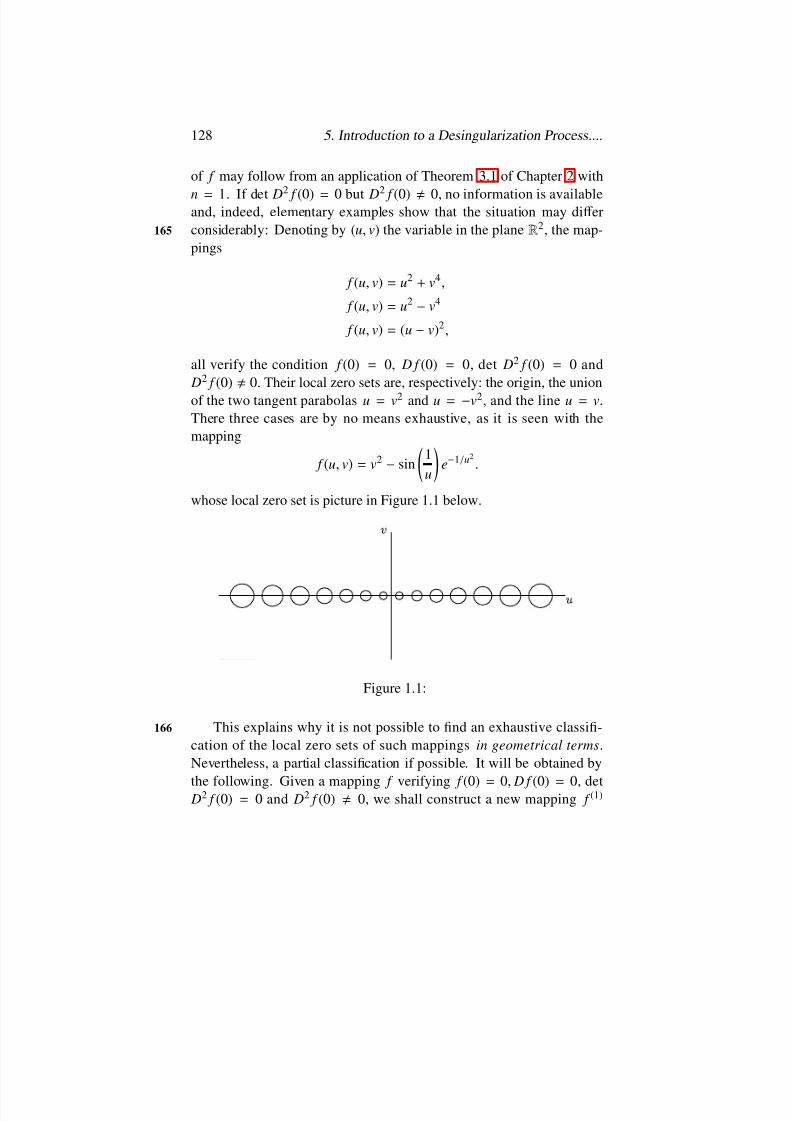
8/2/2019 Rabier-Lectures on Topics in One Parameter Bifurcation Problems
http://slidepdf.com/reader/full/rabier-lectures-on-topics-in-one-parameter-bifurcation-problems 138/238
128 5. Introduction to a Desingularization Process....
of f may follow from an application of Theorem 3.1 of Chapter 2 with
n = 1. If det D2 f (0) = 0 but D
2 f (0) 0, no information is available
and, indeed, elementary examples show that the situation may di ff erconsiderably: Denoting by ( u, v) the variable in the plane R 2 , the map-165
pings
f (u, v) = u2 + v4 ,
f (u, v) = u2−v4
f (u, v) = (u −v)2 ,
all verify the condition f (0) = 0, D f (0) = 0, det D2 f (0) = 0 and D2 f (0) 0. Their local zero sets are, respectively: the origin, the unionof the two tangent parabolas u = v2 and u = −v2 , and the line u = v.There three cases are by no means exhaustive, as it is seen with themapping
f (u, v) = v2 −sin1u
e−1/ u2.
whose local zero set is picture in Figure 1.1 below.
Figure 1.1:
This explains why it is not possible to nd an exhaustive classi-166
cation of the local zero sets of such mappings in geometrical terms .Nevertheless, a partial classication if possible. It will be obtained by
the following. Given a mapping f verifying f (0) = 0, D f (0) = 0, det D2 f (0) = 0 and D2 f (0) 0, we shall construct a new mapping f (1)

8/2/2019 Rabier-Lectures on Topics in One Parameter Bifurcation Problems
http://slidepdf.com/reader/full/rabier-lectures-on-topics-in-one-parameter-bifurcation-problems 139/238
5.1. Formulation of the Problem and Preliminaries. 129
whose local zero set provides that of f through an elementary trans-
fomation. About the mapping f (1)
, the following three possiblities areexhaustive :
1) D f (1) (0) 0 so that the local zero set of f (1) can be found throughthe Implicit function theorem.
2) D f (1) (0) = 0, det D2 f (1) (0) 0 so that the local zero set of f (1)
can be found through the Morse lemma.
3) D f (1) (0) = 0, det D2 f (1) (0) = 0 and D2 f (1) (0) 0 so that ndingthe local zero set of f (1) reduces to nding the local zero set of anew iterate f (2) .
In so doing, we dene a sequence of iterates f (1) , · · ·, f (m) : Theiterate f (m) exists under the necessary and su fficient condition that thelocal zero set of f (m−1) cannot be found through the Implicit functiontheorem or the Morse lemma. If the process ends after a nite numberof steps, it corresponds to a desingularization of the initial mapping f .If it is endless, there are two possibilities, among which one of thembears a geometric characterization (see §8).
We shall complete this section by giving a denition and establish-ing a preliminary property. Of course, the mapping f will henceforth 167
verify the condition f (0) = 0 and
D f (0) = 0, (1.1)detD 2 f (0) = 0, (1.2)
D2 f (0) 0. (1.3)
In particular, (1.2 ) means that the null-space of the mapping D2 f (0) L (R 2 , L (R 2 , R )) does not reduce to 0. Because of ( 1.3), this null-space is not the whole space R 2 and it is then one-dimensional.
Denition 1.1. The one-dimensional space
Ξ = Ker D2 f (0),
will be called the characteristic of f .

8/2/2019 Rabier-Lectures on Topics in One Parameter Bifurcation Problems
http://slidepdf.com/reader/full/rabier-lectures-on-topics-in-one-parameter-bifurcation-problems 140/238
130 5. Introduction to a Desingularization Process....
The following elementary result will be used several times.
Lemma 1.1. Under our assumptions, D 2 f (0) ·( ξ )2 = 0 for some ξ R 2
if and only if ξ Ξ .
Proof. It is obvious that D2 f (0) ·( ξ )2 = 0, if ξ Ξ . Conversely, let ξ R 2
be such that D2 f (0) ·( ξ )2 = 0 and assume by contradiction that there isτ R 2 with D2 f (0) ·( ξ, τ ) 0. Necessarily, ξ and τ are not collinear, sothat ξ, τis a basis of R 2. With respect to this basis, D2 f (0) becomes
0 D2 f (0) ·( ξ, τ ) D2 f (0) ·( ξ, τ ) D2 f (0) ·(τ )2
and its determinant is −( D2 f (0) · ( ξ, τ ))2 < 0, which contradicts the168
hypothesis that it vanishes 2 .
5.2 Desingularization by Blowing-up Procedure.
We shall begin with an approach we have already used in Chapter 2.Extending (in theory) the mapping f to the whole space R 2 as a C ∞mapping, we rst reduce the problem of nding the non-zero solutionsof the equation f ( x) = 0 with prescribed euclidian norm || x||to the prob-lem
(t , x) (R − 0) ×S 1 ,
g(t , ξ ) = 0,(2.1)
where the mapping g dened on R ×R 2 with values in R 2 is given by
g(t , ξ ) =1t 2 f (t ξ ) if t 0,12 D
2 f (0) ·( ξ )2 if t = 0.(2.2)
The relationship of the nonzero solutions x of the equation f ( x) = 0to the solutions ( t , ξ ) of the equation g(t , ξ ) = 0 is of course that x can
always be written as x = t ξ (in two di ff erent ways).

8/2/2019 Rabier-Lectures on Topics in One Parameter Bifurcation Problems
http://slidepdf.com/reader/full/rabier-lectures-on-topics-in-one-parameter-bifurcation-problems 141/238
5.2. Desingularization by Blowing-up Procedure. 131
Remark 2.1. The mapping g in (2.2 ) diff ers from that of Chapter 2 by
the multiplicative factor 1 / 2 only. This modication will bring some169simplications in the formulas later.
Writing the Taylor expansion of f about the origin, we nd that
g(t , ξ ) =
1
0
(1 −s) D2 f (st ξ ) ·( ξ )2ds , (2.3)
for every ( t , ξ ) R ×R 2 , which shows that the mapping g is of class C ∞.The next result, very similar to Lemma 3.2 of Chapter 2, is based on
the observation that the intersectionS
1 ∩Ξ
reduces to two points. Forthe sake of convenience, we shall say that two problems are equivalent if all the solutions of one of them provide all the solutions of the other.We leave it to the reader to keep track of the (obvious) correspondencebetween the solutions of the problems under consideration.
Lemma 2.1. Let ξ 0 be either point of the intersection Ξ ∩S 1 and C a given neighbourhood of ξ 0 in S 1 . Then, for r > 0 small enough the problems
0 < |t | < r , ξ S 1 ,
g(t , ξ ) = 0,(2.4)
and 0 < |t |< r , ξ C ,
g(t , ξ ) = 0,(2.5)
are equivalent.
Proof. First, note that the problem ( 2.5 ) is equivalent to 170
0 < |t |< r , ξ C (−C )
g(t , ξ ) = 0,(2.6)
2Recall that the condition det D2 f (0) = 0 is independent of the choice of any basisin R 2 .

8/2/2019 Rabier-Lectures on Topics in One Parameter Bifurcation Problems
http://slidepdf.com/reader/full/rabier-lectures-on-topics-in-one-parameter-bifurcation-problems 142/238
132 5. Introduction to a Desingularization Process....
since each solution of ( 2.5 ) is obviously a solution of ( 2.6 ) and con-
versely, given any solution ( t , ξ ) of (2.6 ), either ( t , ξ ) or (−t , − ξ ) is asolution of ( 2.5) from the relation g(t , ξ ) = g(−t , − ξ ). We shall prove theassertion by showing that the problems ( 2.4) and (2.6 ) have the samesolutions for r > 0 small enough. Each solution of (2.6 ) is clearly asolution of ( 2.4) . Conversely, assume, by contradiction, that there is nor > 0 such that each solution of ( 2.4 ) is a solution of ( 2.6). This meansthat there is a sequence ( t ℓ , ξ ℓ )ℓ ≥1 with lim
ℓ →+∞t ℓ = 0, ξ ℓ S 1 C (−C ) and
g(t ℓ , ξ ℓ ) = 0. From the compactness of S 1 , we may assume that thereis ξ S 1 such that ξ ℓ converges to ξ . By the coninuity of g, we deduceg(0, ξ ) = 0. But, by denition of g(0, ·) and Lemma 1.1, ξ must be oneof the elements ξ 0 or
− ξ 0 , which is impossible, since ξ ℓ C (
−C ) for
every ℓ ≥1, by hypothesis.
Let us now consider a subspace T of R 2 such that
R 2 = −Ξ T . (2.7)
Given a non-zero element τ 0 T , we may write T = R τ 0 . Let Φ :R 2 →R ×S 1 be the C ∞mapping dened by
Φ (u1 , v1) = (u1|| ξ 0 + v1τ 0||, ( ξ 0 + v1τ 0)/ || ξ 0 + v1τ 0||), (2.8)
(where | · |still denotes the euclidean norm). Clearly, Φ (0, 0) = (0, ξ 0)171
and an elementary calculation yields
DΦ (0, 0) ·(u1 , v1) = (u1 , v1τ 0 −v1 ( ξ 0|τ 0) ξ 0),
for (u1 , v1) R 2 , where ( ·|·) denotes the inner product of R 2. The aboverelation shows that the mapping DΦ (0, 0) is one-to-one (as an elementof L (R 2 , R 3)) and hence is an isomorphism of R 2 to R ×T ξ 0 S 1(= R × ξ 0 ). Thus, Φ is a C ∞diff eomorphism between a neighbourhood of the origin in R 2 and a neighbourhood of the point (0 , ξ 0 ) in R ×S 1 . We
can suppose that the latter contains the product ( −r , r ) ×C of Lemma2.1: it suffices to choose C small enough and shrink r > 0 accordingly.

8/2/2019 Rabier-Lectures on Topics in One Parameter Bifurcation Problems
http://slidepdf.com/reader/full/rabier-lectures-on-topics-in-one-parameter-bifurcation-problems 143/238
5.2. Desingularization by Blowing-up Procedure. 133
Then, Φ−1 ((−r , r ) ×C ) is a neighbourhood W 1 of the origin in R 2 and
each pair ( t , ξ ) (−r , r )×has the form
t = u1|| ξ 0 + v1τ 0||, ξ = ( ξ 0 + v1τ 0)/ || ξ 0 + v1τ 0||,
with ( u1 , v1) W 1 . As t = 0 if and only if u 1 = 0 and from lemma 2.1 .our initial problem of nding the nonzero solutions x in the local zeroset of f is equivalent to
(u1 , v1) W 1 , u1 0,
g(u1|| ξ 0 + v1τ 0||, ( ξ 0 + v1τ 0)/ || ξ 0 + v1τ 0||) = 0
Coming back to the denition of g ((2.2 )), this also reads 172
(u1 , v1) W 1 , u1 0,
f (u1 ( ξ 0 + v1τ 0)) = 0.
Finally, multipying by 1 / u21 , the problem becomes
(u1 , v1 ) W 1 , u1 0,
g(u1 , ξ 0 + v1τ 0) = 0.
We shall denote by f (1) the C ∞real-valued function of two variables
f (1) : (u1 , v1) R 2 →f (1) (u1 , v1 ) = g(u1 , ξ 0 + v1τ 0)
=1u2
1 f (u1 ξ 0 + u1v1τ 0) if u1 0,
12 v2
1 D2 f (0) ·( ξ 0)2 if u1 = 0.
(2.9)
From the above comments, the nonzero solutions x of the equation f ( x) with || x||< r are of the form
x = u1 ξ 0 + u1v1τ 0 (2.10)
with ( u1 , v1) W 1 , u1 0 and f (1)
(u1 , v1 ) = 0. Obviously, the character-ization ( 2.10 ) remains true with the solution x = 0 since f (1) (0, 0) = 0.

8/2/2019 Rabier-Lectures on Topics in One Parameter Bifurcation Problems
http://slidepdf.com/reader/full/rabier-lectures-on-topics-in-one-parameter-bifurcation-problems 144/238
134 5. Introduction to a Desingularization Process....
In other words, since the neighbourhood W 1 = Φ −1((−r , r ) ×C ) can be
taken arbitrarily small (by shrinking C and r > 0), the problem reducesto nding the local zero set of f (1) , from which the local zero set of isdeduced through the transformation ( 2.10) .
Remark 2.2. The reader may wonder why we have not dened the map-173
ping f (1) by formula ( 2.9 ) directly. Indeed, it is clear that every elementof the form (2.10 ) with ( u1 , v1 ) in the local zero set of f (1) is in the localzero set of f . But the problem is to show that every element in the localzero set of f is of the form (2.10 ) with ( u1 , v1) in the local zero set of f (1) , a fact that uses the compactness of the unit circle S 1 , essential inLemma 2.1.
COMMENT 2.1. The vector ξ 0 Ξ has been chosen so that ξ 0 S 1 i.e.
|| ξ 0||= 1. This is without importance and ξ 0 can be taken as an arbitrarynon-zero element of the characteristic Ξ (bu changing the inner productof R 2 for instance). From now on, we shall allow this more generalchoice in the denition of the mapping f (1) in (2.9 ).
All the derivatives of the mapping f (1) can be explicitly computedin terms of the derivatives of f at the origin. First from (2.9 ), for everypair ( j, ℓ ) N ×N
(∂ j+ ℓ f (1) /∂ u j1∂vℓ
1)(0) = (∂ j+ ℓ g/∂ t j∂ ξ ℓ )(0 , ξ 0)
·(τ 0 )ℓ .
Now
Lemma 2.2. For every pair ( j, ℓ ) N ×N , one has
(∂ j+ ℓ f g/∂ t j∂ ξ ℓ )(0 , ξ ) =
0 if ℓ > j + 2
[ j!/ ( j + 2 −ℓ )!] D j+ 2 f (0) ·( ξ ) j+ 2−ℓ
if 0 ≤ℓ ≤ j + 2,
(2.11)
for every ξ R 2 .
Proof. Using the expression ( 2.3 ) of g and for every pair ( t , ξ ) R ×R 2 ,174
8/2/2019 Rabier-Lectures on Topics in One Parameter Bifurcation Problems
http://slidepdf.com/reader/full/rabier-lectures-on-topics-in-one-parameter-bifurcation-problems 145/238
5.3. Solution Through the Implict Function.... 135
we nd
(∂ jg/∂ t j)(t , ξ ) =
1
0
(1 −s)s j D j+ 2 f (st ξ ) ·( ξ ) j+ 2ds .
In particular, for t = 0,
(∂ jg/∂ t j)(0 , ξ ) = −1( j + 1)( j + 2)
D j+ 2 f (0) ·( ξ ) j+ 2 ,
and (2.11 ) follows.
With Lemma 2.2, we obtain for every pair ( j, ℓ ) N ×N ,
(∂ j+ ℓ f (1) /∂ u j1∂vℓ
1)(0) =
0 if ℓ > j + 2,
[ j!/ ( j + 2 −ℓ )!] D j+ 2 f (0) ·(( ξ 0) j+ 2−ℓ ,
(τ 0 )ℓ ) if 0 ≤ℓ < j + 2.(2.12)
In particular, taking j = 0 and ℓ = 2 in formula (2.12 ),
(∂2 f (1) /∂ v21)(0) = D2 f (0) ·(τ 0)2 0, (2.13)
since τ 0 Ξ (cf. Lemma 1.1) .
5.3 Solution Through the Implict Function Theo-rem : CUSP Bifurcation
Applying fromula ( 2.12) with j = 1, ℓ = 0 and j = 0, ℓ = 1 successively,we get
(∂ f (1) /∂ u1)(0) =16 D3 f (0) ·( ξ 0)3 (3.1)
and(∂ f (1) /∂ v1 )(0) =
12 D2 f (0) ·( ξ 0 , τ 0).
But, as ξ 0 Ξ , D2 f (0)
• ξ 0 = 0. Hence 175
(∂ f (1) /∂ v1)(0) = 0. (3.2)

8/2/2019 Rabier-Lectures on Topics in One Parameter Bifurcation Problems
http://slidepdf.com/reader/full/rabier-lectures-on-topics-in-one-parameter-bifurcation-problems 146/238
136 5. Introduction to a Desingularization Process....
From ( 3.1)-(3.2 ), the Implict function theorem can be used for nd-
ing the local zero set of f (1)
if and only if D3 f (0) ·( ξ 0)3 0, (3.3)
a condition which is independent of the nonzero element ξ 0 Ξ and of thespace T chosen for dening the mapping f (1) . Assume then that ( 3.3 )holds. The Implict function theorem states that the local zero set of f (1)
is made of exactly one curve of class C ∞. Due to (3.2 ), this curve istangent to the v1 -axis at the origin. In other words, around the origin
f (1) (u1 , v1) = 0 u1 = u1(v1), u1 (0) = (du 1 / dv1 )(0) = 0.
This result can be made more precise by showing that ( d 2 u1 / dv21 )
(0) 0: Diff erentiating two times the identity f (1) (u1(v1 ), v1) = 0 andsince ( du 1 / dv1)(0) = (∂ f (1) /∂ v1)(0) = 0, we obtain
(d 2u1 / dv21 )(0) = −
(∂2 f (1) /∂ v21)(0)
(∂ f (1) /∂ u1)(0)= −6
D2 f (0) ·(τ 0 )2
D3 f (0) ·( ξ 0)30, (3.4)
as it follows from ( 2.13) . In the (u1 , v1)-plane, the graph of the functionu1(·) is then as in Figure 3.1
Figure 3.1: Local zero set of f (1)
After changing the vector ξ 0 into − ξ 0 if necessary, we may assume176
(cf. ( 3.4) )(d 2u1 / dv2
1 )(0) > 0. (3.5)

8/2/2019 Rabier-Lectures on Topics in One Parameter Bifurcation Problems
http://slidepdf.com/reader/full/rabier-lectures-on-topics-in-one-parameter-bifurcation-problems 147/238
5.3. Solution Through the Implict Function.... 137
Theorem 3.1. The vector ξ 0 being chosen so that (3.5 ) holds, let us set
Ξ+ = R + ξ 0 . Then, the local zero set of f is made up of two continuoushalf-branches emerging from the origin in the half space Ξ + T. Thesehalf-branches are of class C ∞away from the origin and tangent to thecharacteristic Ξ = R ξ 0 at the origin. More precisely, there exists anorigin-preserving C ∞di ff eomorphism ψ in R such that the local zero set of f is made up of the two half-branches ( ρ > 0 small enough) 177
Proof. After changing the vector τ 0 into a scalar multiple, we may as-sume that ( d 2u1 / dv2
1 )(0) = 2 (cf. (3.4) ). Not changing τ 0 introducespositive multiplicative constants in the expressions below without (of course) a ff ecting the nal result. Thus
u1 (v1) = v21(1 + R(v1 )), (3.7)
where R is a C ∞function such that R(0) = 0. The mapping
(v1 ) = v1(1 + R(v1))1/ 2 , (3.8)
is well dened and of class C ∞around the origin. In addition
(0) = 0,d dv1
(0) = 1.
It follows that is an origin-preserving C ∞local di ff eomorphism of R
and the relation ( 3.7 ) is simplyu1 (v1 ) = ( (v1))2 .
From our choice of (3.8 ), we see that
(v1 ) = u1(v1) if v1 > 0,
(v1 ) = − u1(v1) if v1 < 0.
Setting ψ = −1 , we nd
v1 = ψ( u1 (v1 )) if v1 ≥0.
v1 = ψ(
−u1(v1 )) if v1
≤0.
178
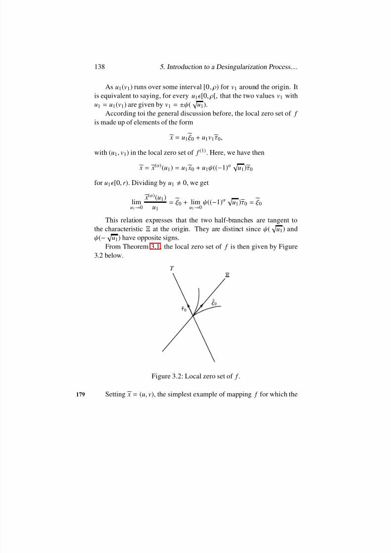
8/2/2019 Rabier-Lectures on Topics in One Parameter Bifurcation Problems
http://slidepdf.com/reader/full/rabier-lectures-on-topics-in-one-parameter-bifurcation-problems 148/238
138 5. Introduction to a Desingularization Process....
As u1 (v1) runs over some interval [0 , ρ) for v1 around the origin. It
is equivalent to saying, for every u1 [0, ρ[, that the two values v1 withu1 = u1 (v1) are given by v1 = ±ψ( √ u1).
According toi the general discussion before, the local zero set of f is made up of elements of the form
x = u1 ξ 0 + u1v1τ 0 ,
with ( u1 , v1) in the local zero set of f (1) . Here, we have then
x = x(α)(u1 ) = u1 x0 + u1ψ((−1)α √ u1 )τ 0
for u1 [0, r ). Dividing by u1 0, we get
limu1→0
x(α )(u1 )u1
= ξ 0 + limu1→0
ψ((−1)α √ u1 )τ 0 = ξ 0
This relation expresses that the two half-branches are tangent tothe characteristic Ξ at the origin. They are distinct since ψ( √ u1) andψ(−√ u1 ) have opposite signs.
From Theorem 3.1, the local zero set of f is then given by Figure3.2 below.
Figure 3.2: Local zero set of f .
Setting x = (u, v), the simplest example of mapping f for which the179

8/2/2019 Rabier-Lectures on Topics in One Parameter Bifurcation Problems
http://slidepdf.com/reader/full/rabier-lectures-on-topics-in-one-parameter-bifurcation-problems 149/238
5.4. Solution Through the Morse Lemma.... 139
hypothesis of this section are fullled is f (u, v) = u2 ±v3 (or v2 ±u2 , or,
with θ any xed real number, ( v cos θ −u sin θ )2
±(u cos θ + v sin θ )3).
This kind of bifurcation is observed in chemical reaction problems (cf.Golubitsky and Keytz [ 13]).
5.4 Solution Through the Morse Lemma : IsolatedSolution and Double Limit Bifurcation.
As we saw in the previous section, a necessary and su fficient conditionfor the local zero set of the mapping f (1) (2.9 ) to be found through theImplicit function theorem is D3 f (0) · ( ξ 0)3 0. Here, we shall then 180
assume D3 f (0) ·( ξ 0 )3 = 0. (4.1)
As a result, from ( 3.1) and (3.2)
(∂ f (1) /∂ u1)(0) = (∂ f (1) /∂ v1)(0) = 0. (4.2)
Let us now examine the second derivative.Taking j = 2ℓ = 0 and j = 1, ℓ = 1 successively in ( 2.12) , we nd
(∂2 f (1) /∂ u21)(0) =
112
D4 f (0) ·( ξ 0)4, (4.3)
(∂2 f (1) /∂ u1∂v1)(0) =12 D3 f (0) ·(( ξ 0 )3, τ 0 ) (4.4)
and we already know that (cf. ( 2.13 ))
(∂2 f (1) /∂ v21)(0) = D2 f (0) ·(τ 0 )2 0. (4.5)
Therefore, the structure of the local zero set of the mapping f (1) canbe found through the Morse lemma if and only if the determinant det D2 f (1) (0) is 0. From the above, this becomes
detD 2 f (1) (0) =1
12( D4 f (0) ·( ξ 0)4)( D2 f (0) ·(τ 0)2) −
14
( D3 f (0) ·( ξ 0)2 , τ 0)2 0.
(4.6)
8/2/2019 Rabier-Lectures on Topics in One Parameter Bifurcation Problems
http://slidepdf.com/reader/full/rabier-lectures-on-topics-in-one-parameter-bifurcation-problems 150/238
8/2/2019 Rabier-Lectures on Topics in One Parameter Bifurcation Problems
http://slidepdf.com/reader/full/rabier-lectures-on-topics-in-one-parameter-bifurcation-problems 151/238
5.4. Solution Through the Morse Lemma.... 141
ξ 0 , τ 0is a basis of R 2 , it suffices to show with ξ = λτ 0, λ R , that the
equations (4.7 ) have no solution other than t = λ = 0. With ( 4.8 )-(4.10 ),they become
t 12 D4 f (0) ·( ξ 0)4 + λ
2 D3 f (0) ·(( ξ 0)2 , τ 0) = 0 R ,t 2 D
3 f (0) ·( ξ 0 )2 + λ D2 f (0) ·τ 0 = 0 L (R 2 , R ).(4.11)
The second equation ( 4.11 ) is equivalent to two scalar equations,obtained, for instance, by expressing that the value of the left hand sidevanishes at each of the two noncollinear vectors ξ 0 and τ 0 . By the samearguments as above (i.e. ( 4.1 ) and ξ 0 Ξ)the rst scalar equation is thetrivial one 0 = 0. The second equation is
t 2 D3 f (0) ·(( ξ 0)2, τ 0 ) + λ D2 f (0) ·(τ 0)2 = 0. (4.12)
But the system made of ( 4.12 ) and the rst equation ( 4.11 ) has theunique solution t = λ = 0 if and only if det D2 f (1) (0) 0 (cf. ( 4.6)),which completes the proof.
Remark 4.1. If D f (1) (0) 0 (i.e. D3 f (0) ·( ξ 0)3 0), it is not true thatthe condition det D2 f (1) (0) 0 is independent of the choice of T , as thereader can easily check on formula ( 4.6) .
Remark 4.2. We could already make Proposition 4.1 more precise byshowing that the sign of det D2 f (1) (0) is independent of the choice of T 183
(when D f (1) (0) = 0) but this will be an immediate consequence of ourfurther analysis.
Theorem 4.1. Assume that D f (1) (0) = 0.
(i) If det D 2 f (1) (0) > 0 , i.e.
13
( D4 f (0) ·( ξ 0)4)( D2 f (0) ·(τ 0)2) −( D3 f (0) ·(( ξ 0)2 , τ 0))2 > 0,
the local zero set of f reduces to the origin.
(ii) If det D 2 f (1) (0) < 0 , i.e.
13
( D4 f (0) ·( ξ 0)4)( D2 f (0) ·(τ 0)2) −( D3 f (0) ·(( ξ 0)2 , τ 0))2 < 0,

8/2/2019 Rabier-Lectures on Topics in One Parameter Bifurcation Problems
http://slidepdf.com/reader/full/rabier-lectures-on-topics-in-one-parameter-bifurcation-problems 152/238
142 5. Introduction to a Desingularization Process....
the local zero set of f consists of exactly two distinct curves of
class C ∞ , tangent to the characteristic Ξ at the origin. More pre-cisely, there exist two real-valued functions v (α)
1 (u1 ), α = 1, 2 , de- ned and of class C ∞around the origin, verifying
dv (1)1
du 1(0)
dv(2)1
du 1(0), (4.13)
such that the local zero set of f is made up of the two curves ( ρ > 0small enough)
u1 (− ρ, ρ) → x(α )(u1) = u1 ξ 0 + u1v(α )1 (u1)τ 0 , α = 1, 2.
Proof. Recall that the local zero set of f is of the form
x = u1 ξ 0 + u1v1τ 0 ,
with ( u1 , v1 ) in the local zero set of f (1) . The part (i) is then obvious
since the local zero set of f (1)
reduces to the origin.Let us now prove (ii). The local zero set of f (1) is made up of two184
C ∞ curves intersecting transversaly at the origin where their tangentsare the two distinct lines of solutions of the equation
D2 f (1) (0) ·(u1 , v1)2 = 0.
Note that the v1 -axis is never one of these tangents since D2 f (0) ·(τ 0 )2 0. As a result, the projection of either tangent onto the u1 -axis
and along the v1-axis a linear isomorphism and it follow that the two C ∞curves can be parameterized by u1 (cf. Figure 4.1 below)
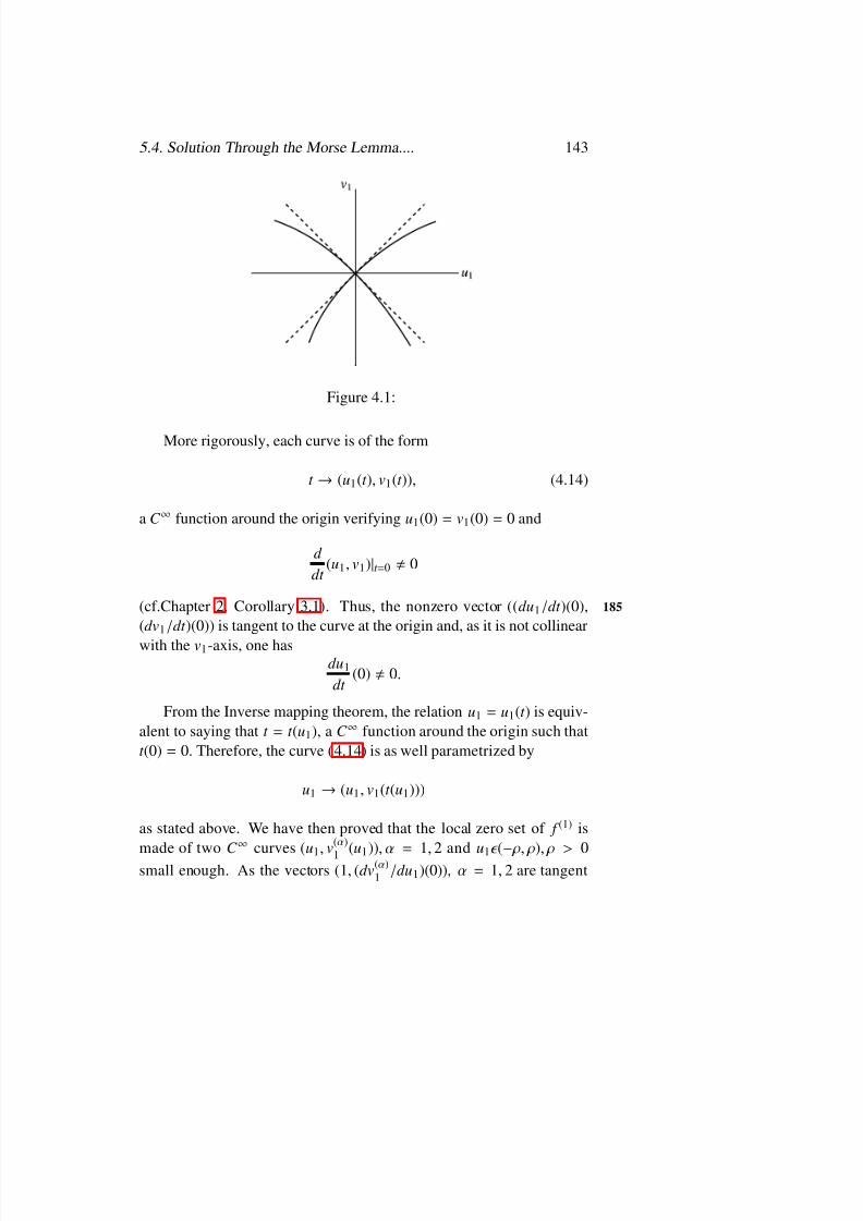
8/2/2019 Rabier-Lectures on Topics in One Parameter Bifurcation Problems
http://slidepdf.com/reader/full/rabier-lectures-on-topics-in-one-parameter-bifurcation-problems 153/238

8/2/2019 Rabier-Lectures on Topics in One Parameter Bifurcation Problems
http://slidepdf.com/reader/full/rabier-lectures-on-topics-in-one-parameter-bifurcation-problems 154/238
144 5. Introduction to a Desingularization Process....
to a diff erent one of the two curves at the origin (and hence are not
collinear) we deduce
dv(1)1
du 1(0)
dv (2)1
du 1(0) .
Finally, the local zero set of f is made of the two C ∞curves
u1 (− ρ, ρ) → x(α)(u1 ) = u1 ξ 0 + u1v(α)1 (u1)τ 0 , α = 1, 2.
Both are tangent to the characteristic Ξ at the origin since
d x(α )
du 1(0) = ξ 0 , α = 1, 2,
and they are distinct, since their second derivatives at the origin186
d 2 x(α)
du 21
(0) =dv(α)
1
du 1(0),
diff er.
Remark 4.3. We get an a posteriori proof of the fact that the sign of det D2 f (1) (0) is independent of the choice of the space T because this signis related to the structure of the local zero set of f .
We shall noe describe a convenient way for nding the local zero setof f from that of f (1) . It wil be repeatedly used in the applications of thenext section and we shall refer to it as the “ quadrant method ”.
Identify the sum Ξ T with the product R ξ 0 ×R τ 0 , the vector τ 0
being chosen so that ξ 0 , τ 0 is a direct system of coordinates. In the
(u1 , v1 )-plane as well as in the product R ξ 0 ×R τ 0 , we shall distinguishthe usual four quadrants (I), (II), (III) and (IV).

8/2/2019 Rabier-Lectures on Topics in One Parameter Bifurcation Problems
http://slidepdf.com/reader/full/rabier-lectures-on-topics-in-one-parameter-bifurcation-problems 155/238

8/2/2019 Rabier-Lectures on Topics in One Parameter Bifurcation Problems
http://slidepdf.com/reader/full/rabier-lectures-on-topics-in-one-parameter-bifurcation-problems 156/238

8/2/2019 Rabier-Lectures on Topics in One Parameter Bifurcation Problems
http://slidepdf.com/reader/full/rabier-lectures-on-topics-in-one-parameter-bifurcation-problems 157/238
5.5. Iteration of the Process. 147
An important observation is that the relation ( ∂2 f (1) /∂ v21)(0) 0
keeps the characteristic Ξ 1 from being the v 1 -axis . This will be summa-rized by saying that the characteristic Ξ 1 is not vertical . Such a notionmakes no sense as far as the characteristic Ξ is concerned, unless wearbitrarily x a system ( u, v) of coordinates in the original plane R 2.
If D f (2) (0) 0, the local zero set of f (2) can be found through theImplicit function theorem. From Theorem 3.1, we deduce the local zeroset of f (1) and, nally, the local zero set of f . If D f (2) (0) = 0 and det D2 f (2) (0) = 0, the mapping f (2) has a characteristic Ξ 2 which is not vertical in its ambient space ( u2 , v2) and the problem reduces to ndingthe local zero set of a third iterate f (3) depending on the new variables(u3 , v3). More generally, we have 190
Theorem 5.1. Assume that the iterates f (1) , · · ·, f (m) are dened and D f (m)(0) 0. After changing ξ 0 into − ξ 0 if necessary and setting Ξ + =R + Ξ , the local zero set of f is made up of two continuous half-branchesemerging from the origin in the half-space Ξ + T . These half-branchesare of class C ∞away from the origin and tangent to the characteristicΞ at the origin.
Proof. The mappings f (1) , · · ·, f (m) are dened after the choice of nonzero elements ξ 0 , · · ·, ξ m−1 and τ 0 , · · ·, τ m−1 in the characteristics Ξ ,Ξ1 , · · ·Ξ m−1 and some given complements T , T 1 , · · ·, T m−1 . In the (u j,v j) plane, ξ j and τ j are of the form ξ j = (α j, β j) and τ j = (λ j, µ j), with
α j 0 since the characteristic Ξ j is not vertical for 1 ≤ j ≤m −1.
Clearly, the iterate f (m) is the rst iterate of f (m−1) . Thus, afterchanging ξ m−1 into − ξ m−1 , if necessary (which does not a ff ect the ex-istence of the mth iterate f (m) or the condition D f (m)(0) (0)), we knowfrom Theorem 3.1 that the local zero set of f (m−1) is made up of twohalf-branches ( ρ > 0 small enough, ψ an origin-presering C ∞ local dif-feomorphism of R )
0 ≤um < ρ − x(α)m−1 (um) = um ξ m−1 + umψ((−1)α √ um)τ m−1 , α = 1, 2.
In the system ( um−1 , vm−1), this becomes
u(α )m−1 (um) = α m−1um + λm−1umψ((−1)α√ um),
8/2/2019 Rabier-Lectures on Topics in One Parameter Bifurcation Problems
http://slidepdf.com/reader/full/rabier-lectures-on-topics-in-one-parameter-bifurcation-problems 158/238
148 5. Introduction to a Desingularization Process....
v(α)m−1(um) = βm−1um + µm−1umψ((−1)α√ um). (5.4)
The above mappings u(α)m−1(·) and v(α)
m−1(·) are of class C 1 in [0, ρ) with191
(du (α )m−1 / du m)(0) = α m−1 0. (5.5)
Now, from §2, the local zero set of f (m−2) is made of elements of theform
xm−2 = um−1 ξ m−2 + um−1vm−1τ m−2 ,
with ( um−1 , vm−1) in the local zero set of f (m−1) . From ( 5.4), xm−2 = x(α)
m−2(um), α = 1, 2, with
xm−2 (um) = u(α)m−1(um) ξ m−2 + u(α)
m−1(um)v(α )m−1 (um)τ m−2 ,
which, in the system ( um−2 , vm−2), expresses as
u(α )m−2 (um) = α m−2u(α )
m−1 (um) + λm−2u(α)m−1 (um)v(α )
m−1(um),
v(α )m−2(um) = βm−2u(α)
m−1(um) + µm−2u(α )m−1 (um)v(α)
m−1(um).
The mappings u(α )m−2 (·)v
(α)m−2(·) are of class C 1 in (0 , ρ) and, from ( 5.5 )
(du (α )m−2 .du m)(0) = α m−2α m−1 0, α = 1, 2,
since α m−2 0. Iterating the process, we nd that the local zero set of f is of the form
x(α)(um) = u(α)1 (um) ξ 0 + u(α)
1 (um)v(α)1 (um)τ 0 , α = 1, 2,
where the functions u(α )1 (·) and v(α )
1 (·) are of class C 1 in [0 , ρ), vanish asthe origin and
(du (α )1 / du m)(0) = α 1 · · ·α m−1 0.
After shrinking ρ > 0 if necessary, the sign of u(α )1 (um) is that of the192
product α 1 · · ·α m−1 for 0 < um < ρ and both values α = 1 and α = 2.
Hence our assertion, since all the mappings we have considered are C ∞away from the origin.
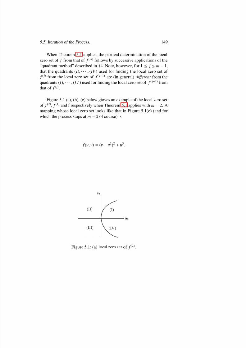
8/2/2019 Rabier-Lectures on Topics in One Parameter Bifurcation Problems
http://slidepdf.com/reader/full/rabier-lectures-on-topics-in-one-parameter-bifurcation-problems 159/238

8/2/2019 Rabier-Lectures on Topics in One Parameter Bifurcation Problems
http://slidepdf.com/reader/full/rabier-lectures-on-topics-in-one-parameter-bifurcation-problems 160/238

8/2/2019 Rabier-Lectures on Topics in One Parameter Bifurcation Problems
http://slidepdf.com/reader/full/rabier-lectures-on-topics-in-one-parameter-bifurcation-problems 161/238
5.5. Iteration of the Process. 151
For m = 1, this was shown in §3 (and the result is obvious). The proof
of this assertion for any m is very technical and will not be given inthese notes (cf. Rabier [ 32])4 . We shall only give the example of thecase when m = 2; The iterate f (2) is dened under the conditions ( 5.1 )and (5.2 ), namely (cf. §§3 and 4)
D3 f (0) ·( ξ 0)3 = 0, (5.6)13
( D4 f (0) ·( ξ )4)( D2 f (0) ·(τ 0)2) −( D3 f (0) ·(( ξ 0 )2 , τ 0))2 = 0. (5.7)
Now, a nonzero element ξ 1 of the characterisitc Ξ 1 is
ξ 1 = ( D2 f (0) ·(τ 0 )2), −12 D3 f (0) ·(( ξ 0)2 , τ 0)).
From §3, the condition D f (2) (0) 0 is equivalent to
D3 f (1) (0) ·( ξ 1 )3 0.
Using ( 5.7) and formula ( 2.12 ), this can be rewritten as
45
( D5 F (0) ·( ξ 0)5 )( D2 f (0) ·(τ 0 )2) −8( D4 f (0) ·(( ξ 0)3, τ 0 ))( D3 f (0)
·(( ξ 0)2, τ 0)) + 4 D3 f (0)
·( ξ 0 , (τ 0)2)( D4 f (0)
·( ξ 0)4) 0.
(5.8)
When ( 5.6 ) and (5.7) hold (which is independent of the choice of 195
ξ 0 Ξ and τ 0 from Proposition 4.1), it is easy to see that ( 5.8) also isindependent of ξ 0 Ξ and τ 0 . However, the reader can already guess thatproving the intrinsic character of the process by using formulas such as(5.6) -(5.8 ) is impossible in the general case.
Assume now that D f (2) (0) = 0. Then, the local zero set of f (2)
can be found through the Morse lemma and Theorem 4.1 provides thestructure of the local zero set of f (1) , from which the structure of thelocal zero set of f is easily derived. More generally, we have
4However, §6 gives a partial result in this direction.

8/2/2019 Rabier-Lectures on Topics in One Parameter Bifurcation Problems
http://slidepdf.com/reader/full/rabier-lectures-on-topics-in-one-parameter-bifurcation-problems 162/238
152 5. Introduction to a Desingularization Process....
Theorem 5.2. Assume that the iterates f (1) , · · ·, f (m) are dened and
D f (m)
(0) = 0 , det D2 f
(m)(0) 0. Then, the local zero set of f reduces
to the origin if det D 2 f (m)(0) > 0 and is made up of exactly two distinct curves of class C ∞ tangent to the characteristic Ξ at the origin if det D2 f (m)(0) < 0.
Proof. It is possible to parallel the proof of Theorem 5.1 . However, weare going to give a more “geometrical” one. We limit ourselves to thecase m = 2, the general situation being identical by repeating the samearguments. From §2 we know that the local zero set of f is of the form
x = u1 ξ 0 + u1v1τ 0 ,
with ( u1 , v1) in the local zero set of f (1) . The assertion is then obvious if 196det D2 f (2) (0) > 0 since the local zero set of f (1) reduces to the origin (cf.Theorem 4.1). Assume then that det D2 f (2) (0) < 0 so that the local zeroset of f (1) is made of two C ∞curves tangent to the characteristic Ξ1 atthe origin as Theorem 4.1 states. In addition, from the proof of Theorem4.1, these curves coincide with the graphs of two C ∞functions denedaround the origin in Ξ 1 with values in T 1 . The important point is thatthis property is not a ff ected, if T 1 is replaced by any other complementof T 1 (express the general form of a linear change of coordinates leav-ing the characteristic Ξ 1 globally invariant and use the Implicit functiontheorem). In particular, as the characteristic Ξ1 is not vertical, this com-
plement can be taken as the v1-axis R (0, 1). Thus, the local zero set of f (1) coincides with the graphs of two C ∞ functions dened around theorigin Ξ 1 with values in R (0, 1). Because the characterisitc Ξ 1 is notvertical again, its projection onto the u1 -axis is a linear isomorphism. Itfollows that the local zero set of f (1) coincides with the graphs of twoC ∞functions v(α)
1 (u1 ), α = 1, 2, dened for |u1| < ρ ( ρ > 0 small enough)verifying v(α)
1 (0) = 0. Hence, the local zero set of f is made up of thetwo curves
u1 (− ρ, ρ) → x(α)(u1 ) = u1 ξ 0 + u1v(α)1 (u1)τ 0 , α = 1, 2.
Theses two curves are tangent to the characteristic Ξ at the originand they are distinct, since they coincide with the graphs of the two
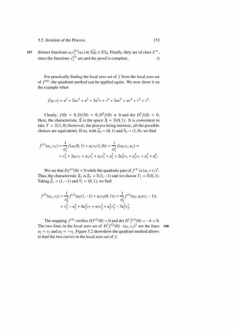
8/2/2019 Rabier-Lectures on Topics in One Parameter Bifurcation Problems
http://slidepdf.com/reader/full/rabier-lectures-on-topics-in-one-parameter-bifurcation-problems 163/238
5.5. Iteration of the Process. 153
distinct functions u1v(α)1 (u1 ) in R ξ 0 ×R τ 0. Finally, they are of class C ∞,197
since the functions v(α )1 are and the proof is complete.
For practically nding the local zero set of f from the local zero setof f (m) , the quadrant method can be applied again. We now show it onthe example when
f (u, v) = u2 + 2uv2 + u3 + 2u2v + v4 + 2uv3 + uv4 + v5 + v6 .
Clearly, f (0) = 0, D f (0) = 0, D2
f (0) 0 and det D2
f (0) = 0.Here, the characteristic Ξ is the space Ξ = R (0, 1). It is convenient totake T = R (1, 0) (however, the process being intrinsic, all the possiblechoices are equivalent). If so, with ξ 0 = (0, 1) and τ 0 = (1, 0), we nd
f (1) (u1 , v1 ) =1u2
1
f (u1(0, 1) + u1v1(1, 0)) =1u2
1
f (u1v1 , u1 ) =
= v21 + 2u1v1 + u1v3
1 + u1v21 + u2
1 + 2u21v1 + u3
1v1 + u31 + u4
1 .
We see that D f (1) (0) = 0 while the quadratic part of f (1) is (u1 + v1)2 .Thus, the characteristic Ξ 1 is Ξ 1 = R (1, −1) and we choose T 1 = R (0, 1).Taking ξ 1 = (1, −1) and τ 1 = (0, 1), we nd
f (2) (u2 , v2 ) =1u2
2
f (1) (u2 (1, −1) + u2v2(0, 1)) =1u2
2
f (1) (u2 , u2 (v2 −1))
= v22 −u2
2 + 4u22 v2 + u2v2
2 + u22v3
2 −3u22v2
2 .
The mapping f (2) veries D f (2) (0) = 0 and det D2 f (2) (0) = −4 < 0.The two lines in the local zero set of D2 f (2) (0) · (u2 , v2)2 are the lines 198
u2 = v2 and u2 = −v2 . Figure 5.2 showshow the quadrant method allowsto nd the two curves in the local zero set of f .
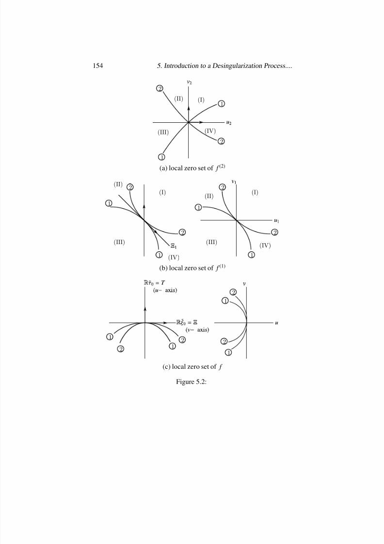
8/2/2019 Rabier-Lectures on Topics in One Parameter Bifurcation Problems
http://slidepdf.com/reader/full/rabier-lectures-on-topics-in-one-parameter-bifurcation-problems 164/238
154 5. Introduction to a Desingularization Process....
(II) (I)
(III) (IV)
2
1
1
2
(a) local zero set of f (2)
(II)(I)
(III)
(IV)
2
1
1
2
(II) (I)
(III) (IV)
2
1
1
2
(b) local zero set of f (1)
2 1
12
2
1
1
2
(c) local zero set of f
Figure 5.2:

8/2/2019 Rabier-Lectures on Topics in One Parameter Bifurcation Problems
http://slidepdf.com/reader/full/rabier-lectures-on-topics-in-one-parameter-bifurcation-problems 165/238
5.6. Partial Results on the Intrinsic Character of the Process 155
5.6 Partial Results on the Intrinsic Character of the
Process
A natural question we have already mentioned is to know whether the 199
process described in §5 is intrinsic or depends on the successive spacesT , T 1 , · · ·, T m−1 and elements ξ 0 , ξ 1 , · · ·, ξ m−1 and τ 0, τ 1 , · · ·, τ m−1 cho-sen for dening the iterates f (1) , · · ·, f (m) . In §3, we saw that the con-dition D f (1) (0) 0 was independent of the choice of T and ξ 0 , τ 0 andwe also proved a similar result as concerns the conditions D f (1) (0) = 0and det D2 f (1) (0) 0 together (cf. Proposition 4.1). The existence of asecond iterate f (2) (i.e. the condition D f (1) (0) = 0, det D2 f (1) (0) = 0)is then independent of T and ξ 0, τ 0 . Given such a space T and elements ξ 0 Ξ , τ 0 T from which f (1) is dened, the existence of a third iterate f (3) is then independent of the choice of the complement T 1 of the char-acteristic Ξ 1 and of the non-zero elements ξ 1 Ξ 1 , τ 1 T 1 . But whether ornot its existence is independent of the initial choice of T and ξ 0 , τ 0 is not ensured by our previous results . However, we can reduce the question asfollows. Since the characteristic Ξ1 is not vertical and since the result isknown to be independent of T 1 , it suffices to prove that the existence of f (3) is independent of T , ξ 0, τ 0 when T 1 is taken as the v 1-axis. Supposethen that this step has been solved successfully. We deduce that the ex-istence of a fourth iterate f (4) is independent of the choice of T 1 , T 2 and 200
of the non-zero elements ξ 1 , ξ 2 and τ 1 , τ 2 in the characterisitcs Ξ 1 , Ξ 2
and their complements T 1 , T 2 respectively. Again, the non-dependenceon the initial choice of T and ξ 0 , τ 0 is not a consequence of the resultswe have established so far, but the problem can be reduced to the casewhen T 1 is taken as the v1-axis and T 2 is taken as the v2 -axis. Moregenerally, we see that proving that the process of §5 is intrinsic reducesto proving for every m that it is independent of T and ξ 0 , τ 0 when thespace T 1 , · · ·, T m−1 are taken as the v1−, · · ·, vm−1-axes.
Therefore, we shall henceforth assume that the sequence f (1) , . . . , f (n) is dened when T j is taken as the v j-axis , 1 ≤ j ≤m −1. Equiva-lently, we shall say that each space T j, 1 ≤ j ≤m−1 is vertical . A proof
of the independence of T based on some generalization of Proposition4.1 is not available. Indeed, Proposition 4.1 allows to prove the rst in-

8/2/2019 Rabier-Lectures on Topics in One Parameter Bifurcation Problems
http://slidepdf.com/reader/full/rabier-lectures-on-topics-in-one-parameter-bifurcation-problems 166/238
156 5. Introduction to a Desingularization Process....
dependence result and is based on “linear” arguments while the question
of the independence of T in the general case is a higher order (hence)nonlinear problem. By showing that the two half-branches / curves (fol-lowing that either Theorem 5.1 or Theorem 5.2 applies) in the local zeroset of f have a contact of order m exactly at the origin, it is possible toestablish that the process is intrinsic if, for choice of T , D f (m)(0) 0 or D f (m)(0) = 0 and det D2 f (m)(0) < 0 (thus, in such a case, m and eithercondition D f (m)(0) 0 or D f (m)(0) = 0 and det D2 f (m)(0) < 0 is inde-pendent of T ). If D f (m)(0) = 0 and det D2 f (m)(0) > 0, the local zeroset of f reduces to the origin and no useful information of an invariant201
geometrical character can be derived from the structure of the local zeroset of f . Neverthless, this situation also can be shown to be intrinsic.
The details of the above assertions can be found in Rabier [ 32]. Here, itwill be su fficient for our purposes to prove that the process is intrinsicin a particular case that we shall now describe.
We begin with a denition. We shall say that the characteristic Ξ j
is horizontal if it coincides with u j-axis in its ambient space ( u j, v j).Similarly, after the choice of a system of coordinates ( u, v) in the orig-inal plane R 2 , we shall say that the characteristic Ξ is horizontal if itcoincides with the u-axis. The v-axis will be referred to as the verticalaxis.
Remark 6.1. Note that we can always make a choice of the system ( u, v)
so that the characteristic Ξ is horizontal but we have no freedom of mak-ing the characteristics Ξ 1 , · · ·, Ξ m−1 horizontal. Conversely, the char-acteristics Ξ 1 , · · ·, Ξ m−1 being horizontal is independent of the system(u, v) of coordinates in the original plane R 2 , since no particular systemis involved in their denition.
Theorem 6.1. Let (u, v) be a system of coordinates in which the charac-teristic Ξ is not vertical. Then, the characteristics Ξ , Ξ 1 , · · ·, Ξm−1 arehorizontal if and only if
(∂ j f /∂ ui)(0) = 0, 0 ≤ j ≤2m, (6.1)
(∂ j+ 1 f /∂ u j∂v)(0) = 0, 0
≤j
≤m. (6.2)
202
8/2/2019 Rabier-Lectures on Topics in One Parameter Bifurcation Problems
http://slidepdf.com/reader/full/rabier-lectures-on-topics-in-one-parameter-bifurcation-problems 167/238
5.6. Partial Results on the Intrinsic Character of the Process 157
Proof. Note that the relations ( 6.1) and (6.2 ) are independent of the
change of coordinates leaving the u-axis invariant. Indeed, such achange of coordinates is of the form
U = au + bv,
V = cv,
with ac 0. Thus, at the origin
∂ j/∂ u j = a j∂ j/∂ U j, ∂ j+ 1/∂ u j∂u = a jb∂ j+ 1 /∂ U j+ 1 + a jc∂ j+ 1 /∂ U j∂V ,(6.3)
so that the relations ( 6.1 ) and (6.2 ) hold in the system ( U , V ) if and onlyif they hold in the system ( u, v).
As the characteristic Ξ is not vertical, it is therefore not restrictive tosuppose that T is the v-axis (by changing the latter, not T ). On the otherhand, the equivalence is true with m = 1 as is immediately checked.Assume then m > 1 and the equivalence holds. We shall prove thatthe characteristics Ξ , Ξ 1 , · · ·, Ξ m exist and are horizontal if and only if (6.1) and (6.2) hold with m + 1 replacing m. Let then the characteristicsΞ , Ξ 1 , · · ·, Ξ m−1 exist and be horizontal. In particular, this is true withΞ , Ξ 1 , · · ·, Ξ m−1 , which is equivalent to ( 6.1 ) - (6.2) by hypothesis. Now,saying that Ξ m exists and is horizontal means that
D f (m)(0) = D2 f (m)(0) ·(1, 0) = 0 L (R 2 , R ),
a condition expressed by the four scalar equations
(∂ f (m)/∂ um)(0) = (∂ f (m)/∂ vm)(0)
= (∂2 f (m)/∂ um∂vm)(0)
= (∂2 f (m)/∂ u2m)(0) = 0.
Applying formula ( 2.12 ) with f (m) , f (m−1) , ξ m−1 and τ m−1 replac- 203
ing f (1) , f , ξ 0 and τ 0 respectively, where ξ m−1 and τ m−1 are two givennonzero elements of Ξ m−1 and T m−1 (= vm−1 -axis), the equation(∂ f (m)/∂ vm)(0) = 0 is automatically satised. The remaining three onesare
D3 f (m−1) (0) ·( ξ m−1)3 = D4 f (m−1) (0) ·( ξ m−1)4
8/2/2019 Rabier-Lectures on Topics in One Parameter Bifurcation Problems
http://slidepdf.com/reader/full/rabier-lectures-on-topics-in-one-parameter-bifurcation-problems 168/238

8/2/2019 Rabier-Lectures on Topics in One Parameter Bifurcation Problems
http://slidepdf.com/reader/full/rabier-lectures-on-topics-in-one-parameter-bifurcation-problems 169/238

8/2/2019 Rabier-Lectures on Topics in One Parameter Bifurcation Problems
http://slidepdf.com/reader/full/rabier-lectures-on-topics-in-one-parameter-bifurcation-problems 170/238
8/2/2019 Rabier-Lectures on Topics in One Parameter Bifurcation Problems
http://slidepdf.com/reader/full/rabier-lectures-on-topics-in-one-parameter-bifurcation-problems 171/238
5.7. An Analytic Proof of Krasnoselskii’s Theorem.... 161
5.7 An Analytic Proof of Krasnoselskii’s Theorem
in a Non-Classical Particular Case.
In this section, we consider again the problem of nding the local zeroset of a mapping of the form
G ( µ, x) = ( I −(λ0 + µ) L) x + Γ ( µ, x), (7.1)
dened on a neighbourhood of the origin in the product R × X and takingits values in the real Banach space X. As in Chapter 1, the operator L L ( X ) is supposed to be compact and the nonlinear operator Γ veries
Γ( µ, 0) = 0, (7.2)
D xΓ( µ, 0) = 0, (7.3)
for | µ| small enough. For the sake of simplicity, we shall assume that Γis of class C ∞, although this hypothesis of regularity can be weakenedwithout a ff ecting the nal results.
Recall the notation introduced in Chapter 1
X 1 = Ker( I −λ0 L), (7.4)
Y 2 = Range ( I −λ0 L) (7.5)
while X 2 and Y 1 are two topological caomplements of X 1 and Y 2 re- 208
spectively. Denoting by Q1 and Q2 the projection operators onto thespaces Y 1 and Y 2, the Lyapunov-Schmidt reduction leads to the reducedequation (cf. Chapter 1, §3)
f ( µ, x) = −µλ0
Q1 x −µλ0
Q1 ( µ, x) + Q1Γ( µ, x + ( µ, x)) = 0, (7.6)
for ( µ, x) around the origin of R × X 1, where the mapping (here of classC ∞) is characterized by
− µλ0
Q2 x+ ( I −λ0 L) ( µ, x)− µQ2 L ( µ, x)+ Q2Γ( µ, x+ ( µ, x)) = 0, (7.7)
and veries the conditions
( µ, 0) = 0 (7.8)

8/2/2019 Rabier-Lectures on Topics in One Parameter Bifurcation Problems
http://slidepdf.com/reader/full/rabier-lectures-on-topics-in-one-parameter-bifurcation-problems 172/238
162 5. Introduction to a Desingularization Process....
for | µ| small enough and
D (0) = 0. (7.9)When the algebraic and geometric multiplicities of λ0 coincide,
namely
X = X 1 Y 2(= Ker( I −λ0 L) Range ( I −λ0 L)), (7.10)
the problem was studied in Chapter 1 if dim Ker ( I −λ0 L) = 1 and inChapter 3 if dim Ker ( I −λ0 L) = n ≥ 2. In what follows, we shallassume
dim Ker( I −λ0 L) = 1, (7.11)
but drop the condition ( 7.10 ). This means that we consider the case209
X 1 Y 2(i.e. Ker ( I −λ0 L) Range ( I −λ0 L)). (7.12)
Thus, for x X 1 , Q1 x = 0 and Q2 x = x so that the reduced mapping(7.6) becomes
f ( µ, x) = − µλ0
Q1 ( µ, x) + Q1Γ( µ, x + ( µ, x)), (7.13)
while the characterization ( 7.7 ) of the mapping can be rewritten as
− µλ0
x+ ( I −λ0l) ( µ, x)− µQ2 L ( µ, x) + Q2Γ( µ, x + ( µ, x)) = 0. (7.14)
The generalized null-space of the operator ( I
−λ0 L) will play a key
role. Recall that it is dened as
Ker( I −λ0 L)γ ,
where γ is the smallest positive integer such that 5
Ker( I −λ0 L)γ ′ = Ker( I −λ0 L)γ ,
for every γ ′ ≥γ . Because of ( 7.12) , one has γ ≥2 and, by denition thealgebraic multiplicity of λ0 is the integer
dim Ker( I −λ0 L)γ .
5The existence of γ is known from the spectral theory of compact operators as re-called in Cahpter 1.
8/2/2019 Rabier-Lectures on Topics in One Parameter Bifurcation Problems
http://slidepdf.com/reader/full/rabier-lectures-on-topics-in-one-parameter-bifurcation-problems 173/238

8/2/2019 Rabier-Lectures on Topics in One Parameter Bifurcation Problems
http://slidepdf.com/reader/full/rabier-lectures-on-topics-in-one-parameter-bifurcation-problems 174/238

8/2/2019 Rabier-Lectures on Topics in One Parameter Bifurcation Problems
http://slidepdf.com/reader/full/rabier-lectures-on-topics-in-one-parameter-bifurcation-problems 175/238
5.7. An Analytic Proof of Krasnoselskii’s Theorem.... 165
Thus, the relations ( 7.21 )-(7.26 ) show that D f (0) = 0, det D2 f (0) =212
0 and D2 f (0) 0. According to Corollary 6.1, it suffices to prove that
there exists an index j (necessarily ≥2) such that ( ∂ j+ 1 f /∂µ j∂ )(0) 0.From (7.23 ), this is equivalent to showing that
Q1∂ j
∂µ j−1∂ (0) 0.
for some j ≥2. To does this, we go back to the characterization of (7.18 ). Diff erentiating this identify with respect to and setting = 0,it follows from ( 7.3) that
−µ
λ0e
0+ ( I
−λ
0 L)
∂
∂ − µQ
2 L
∂
∂ ( µ, 0) = 0.
Now, di ff erentiating with respect to µ yields
−1
λ0e0 + ( I −λ0 L)
∂2
∂µ∂ ( µ, 0) − µQ2 L
∂2
∂µ∂ ( µ, 0) −Q2 L
∂∂
( µ, 0) = 0,
(7.27)which, because of ( 7.9 ), provides
( I −λ0 L)∂2
∂µ∂ (0) =
1λ0
e0 . (7.28)
Assume rst that γ = 2. If Q1 ∂2
∂µ∂ (0) = 0, one has ∂2
∂µ∂ (0) Y 2 = Range ( I −λ0 L). Thus, there exists ξ X such that
( I −λ0 L) ξ =∂2
∂µ∂ (0) . (7.29)
Hence, from ( 7.28 )
( I −λ0 L)2 ξ =1
λ0, (7.30)
and consequently ( I −λ0 L)3 ξ = 0. But, since γ = 2,
Ker ( I −λ0 L)3 = Ker ( I −λ0 L)2 .
8/2/2019 Rabier-Lectures on Topics in One Parameter Bifurcation Problems
http://slidepdf.com/reader/full/rabier-lectures-on-topics-in-one-parameter-bifurcation-problems 176/238
166 5. Introduction to a Desingularization Process....
We deduce that ( I −λ0 l)2 ξ = 0, which contradicts ( 7.30 ). Our as- 213
sertion is then proved when γ = 2. When γ ≥3, we shall use the samemethod but we need some preliminary observations. First, by di ff eren-tiating (7.27 ) at any order j −1, j ≥2, at the origin, we get
( I −λ0 L)∂ j
∂µ j−1∂ (0) = ( j −1)Q2 L
∂ j−1
∂µ j−2∂ (0). (7.31)
If there is 3 ≤ j ≤ γ such that Q1∂ j−1
∂µ j−2∂ (0) 0, the problem issolved. Assume then
Q1∂ j−1
∂µ j
−2∂
(0) = 0, 3 ≤ j ≤γ,
or equivalently,
∂ j−1
∂µ j−2∂ (0) Y 2 = Range ( I −λ0 L), 3 ≤ j ≤γ
Clearly, the space Range ( I −λ0 L) is stable under L and, for theindices 3 ≤ j ≤γ , (7.31 ) reads
( I −λ0 L)∂ j
∂µ j−1∂ (0) = ( j −1) L
∂ j−1
∂µ j−2∂ (0). (7.32)
In particular, for j = γ and applying ( I −λ0 L) to both sides
( I −λ0 L)2 ∂γ∂µγ −1∂
(0) = (γ −1) L( I −λ0 L)∂γ −1
∂µγ −2∂ (0).
If γ = 3, it follows from (7.28 ) that
( I −λo L)2 ∂3
∂µ2∂ (0) =
2λ2
0
e0 ,
while, if γ ≥4, (7.32) provides214
( I −λ0 L)2 ∂γ
∂µγ −1∂ (0) = (γ −1)(γ −2) L2 ∂
γ
−2
∂µγ −3∂ (0).

8/2/2019 Rabier-Lectures on Topics in One Parameter Bifurcation Problems
http://slidepdf.com/reader/full/rabier-lectures-on-topics-in-one-parameter-bifurcation-problems 177/238

8/2/2019 Rabier-Lectures on Topics in One Parameter Bifurcation Problems
http://slidepdf.com/reader/full/rabier-lectures-on-topics-in-one-parameter-bifurcation-problems 178/238

8/2/2019 Rabier-Lectures on Topics in One Parameter Bifurcation Problems
http://slidepdf.com/reader/full/rabier-lectures-on-topics-in-one-parameter-bifurcation-problems 179/238
8/2/2019 Rabier-Lectures on Topics in One Parameter Bifurcation Problems
http://slidepdf.com/reader/full/rabier-lectures-on-topics-in-one-parameter-bifurcation-problems 180/238
170 5. Introduction to a Desingularization Process....
w = ( µ, ) =(1 + µ) −√ ((1 + µ)2 + 4 µ )
2= −
2 µ (1 + µ) + √ ((1 + µ)2 + 4 µ )
,
so that( µ, )− µ ,
around the origin. By referring to the second equation ( 7.37 ), we ndthe reduced mapping f ( µ, ) − µ2 + 2 . The solutions of the equation
− µ2 + 2 = 0 are ( µ, 0) and ( µ, µ2) and the local zero set of f is as inFigure 7.1 with γ even. Note that the “natural” choice
Γ( , v) = ( 2 , v2)
cannot be treated here because the condition ( 7.24 ) fails (and hence D2 f (0) = 0). Actually, the associated reduced equation is
− µ ( µ, ) + 2( µ, ) = 0, (7.38)
with
( µ, ) = ( − µ)1 + µ
It is easily checked that the local zero set of the reduced mapping
is made up of the three transversal curves ( µ, 0), ( µ, µ) and (2 / [1 + +√ ((1 + )2 + 4 2 ) , ) ( 2 , ). Observe in this case that Theorem 4.1of Chapter 2 applies to the reduced mapping ( 7.38 ) because its rstnonzero derivative at the origin is of order 3 and the associated poly-nomial mapping veries the condition ( R − N . D.). This is not in contra-diction with the analysis of Chapter 3, because the condition ( 1.7 ) (as219
well as its generalized form ( 1.26 )) of Chapter 3 fails .
5.8 The Case of an Innite Process.
To be complete, we analyze now the case when the process of §5 isendless. We begin with the following denition

8/2/2019 Rabier-Lectures on Topics in One Parameter Bifurcation Problems
http://slidepdf.com/reader/full/rabier-lectures-on-topics-in-one-parameter-bifurcation-problems 181/238
8/2/2019 Rabier-Lectures on Topics in One Parameter Bifurcation Problems
http://slidepdf.com/reader/full/rabier-lectures-on-topics-in-one-parameter-bifurcation-problems 182/238

8/2/2019 Rabier-Lectures on Topics in One Parameter Bifurcation Problems
http://slidepdf.com/reader/full/rabier-lectures-on-topics-in-one-parameter-bifurcation-problems 183/238
5.8. The Case of an Innite Process. 173
(which does not vanish at the origin).
We shall see how the mapping v is related to the characteristicsΞ , Ξ 1 , · · ·, Ξ m, · · ·With this aim, there is a choice of elements ξ j andτ j, j ≥ 0, that is especially convenient for dening the iterates f ( j) :Let γ 0 be the slope of the characteristic Ξ in the system ( u, v) (recall 222
that γ 0 is well dened as a real number since Ξ is not vertical) and set ξ 0 = (1, γ 0 ). Taking T as the v-axis, we choose τ 0 = (0, 1). The rstiterate f (1) is entirely determined from ξ 0 and τ 0 and its characteristic Ξ 1
is not vertical in the ( u1 , v1 )-plane. Denoting by γ 1 the slope of Ξ 1 , weset ξ 1 = (1, γ 1). Taking T 1 as the v1-axis, we choose τ 1 = (0, 1) whichdetermines the second iterate f (2) . In general, the choice of the ξ j’s andτ j’s is then as follows
ξ j = (1, γ j), j ≥0, (8.4)
where γ j denotes the slope of the characteristic Ξ j in the (u j, v j) planeand
τ j = (0, 1), j ≥0. (8.5)
Remark 8.2. Note for every j ≥1 that the characteristic Ξ j depends on ξ ℓ and τ ℓ , 0 ≤ ℓ ≤ j −1. Thus, by modifying one of the ξ j’s (or τ j’s)we aff ect the denition of all the characteristics of order > j. This isto say that our further results hold with the choice (8.4 )-(8.5 ) and withthis choice only . If any other choice of elements ξ j and τ j is made, therelationship to the characteristics Ξ , Ξ1 , · · ·, Ξ m, · · ·is di ff erent .
Before the rst important theorem of this section, we need to estab-lish
Lemma 8.1. Let m ≥1 be a given integer. We set
ˆ f (u, v) = f u, v +m−1
j= 0
γ ju j+ 1 . (8.6)
223
Then, the characteristicsˆΞ ,
ˆΞ 1 , · · ·,
ˆΞ m−1 of
ˆ f ,
ˆ f
(1)
, · · ·,ˆ
f (m
−1)
exist and are horizontal.

8/2/2019 Rabier-Lectures on Topics in One Parameter Bifurcation Problems
http://slidepdf.com/reader/full/rabier-lectures-on-topics-in-one-parameter-bifurcation-problems 184/238
174 5. Introduction to a Desingularization Process....
Proof. It is clear that D ˆ f (0) = 0. Now, we have
∂2 ˆ f ∂u2 (0) =
∂2 f ∂u2 (0) + 2
∂2 f ∂u∂v
(0)γ 0 +∂2 f ∂v2 (0)γ 20 =
= D2 f (0) ·(1, γ 0)2 = D2 f (0) ·( ξ 0)2 = 0,
and
∂2 ˆ f ∂u∂v
(0) =∂2 f
∂u∂v(0) +
∂2 f ∂v2 (0)γ 0
= D2 f (0) ·((1 , γ 0 ), (0, 1))
= D2 f (0) ·( ξ 0 , τ 0) = 0
Finally, since
∂2 ˆ f ∂v2 (0) =
∂2 f ∂v2 (0) = D2 f (0) ·(0, 1)2 = D2 f (0) ·(τ 0)2 0, (8.7)
the above relations show that the characteristic Ξ of ˆ f exists and is hor-izontal.
Taking ˆ ξ 0 = (1, 0) and τ 0 = τ 0 = (0, 1), the rst iterate ˆ f (1) is denedby
ˆ f (1) (u1 , v1 ) =1u2
1
ˆ f (u1 , u1v1) if u1 0,
12
∂2 ˆ f ∂v2 (0)v2
1 if u1 = 0.(8.8)
By denition, one has
ˆ f (1) (u1 , v1 ) =1u2
1 f (u1 , γ 0u1 + u1v1) if u1 0,
12
∂2 f ∂v2 (0)v2
1 if u1 = 0.(8.9)
Thus, from ( 8.7) -(8.9 ) we deduce224
ˆ f (1) (u1 , v1 ) = f (1) u1,m−1
j= 1
γ ju j1 . (8.10)
Setting γ (1) j = γ j+ 1 , 0 ≤ j ≤m −2,

8/2/2019 Rabier-Lectures on Topics in One Parameter Bifurcation Problems
http://slidepdf.com/reader/full/rabier-lectures-on-topics-in-one-parameter-bifurcation-problems 185/238
5.8. The Case of an Innite Process. 175
we see that γ (1) j , 0 ≤ j ≤m −2 play with f (1) the same role as γ j, 0 ≤
j ≤m −1, play with f . Therefore, it follows from (8.10 ) that the iterateˆ f (1) is dened from f (1) as ˆ f is dened from f . The same observationcan be repeated m −1 times and our assertion follows.
Theorem 8.1. Let f be a reducible ∞-degenerate mapping. The iterate f (1) , · · ·, f (m) , · · ·being dened from ξ j and τ j, j ≥0 as in ( 8.4 )-(8.5) ,the function v (u) whose graph is the local zero set of f veries
d jvdu j (0) = j!γ j−1 for every j ≥1. (8.11)
Conversely, if f is ∞-degenerate and real-analytic and the disk of
convergence of the power series∞
j= 0 γ ju j+ 1
is not 0 , the mapping f isreducible and its local zero set coincides with the graph of the analytic function
v(u) =∞
j= 0
γ ju j+ 1 . (8.12)
Proof. Let m ≥1 be a given integer. Set
v(u) = v(u) −m−1
j= 0
γ ju j+ 1 . (8.13)
With the characterization f (u, v(u)) = 0, we nd 225ˆ f (u, v(u)) = 0, (8.14)
where ˆ f is the mapping ( 8.11 ). From Lemma 8.1, the charactericticsΞ , Ξ 1 , Ξ m−1 , · · ·are horizontal. Thus, using Theorem 6.1,
(∂ j ˆ f /∂ u j)(0) = 0, 0 ≤ j ≤2m,
(∂ j+ 1 ˆ f /∂ u j∂v)(0) = 0, 0 ≤ j ≤m.
By implicit di ff erentiation in ( 8.14 ), it easily follows that ( d jv/ du j)(0) = 0, 0 ≤ j ≤m. By denition of ˆv (cf. (8.13 )), this is equivalent to
d jvdu j (0) = j!γ j−1 , 0 ≤ j ≤m.

8/2/2019 Rabier-Lectures on Topics in One Parameter Bifurcation Problems
http://slidepdf.com/reader/full/rabier-lectures-on-topics-in-one-parameter-bifurcation-problems 186/238
176 5. Introduction to a Desingularization Process....
But this relation holds for any m ≥1, which proves ( 8.11) .
Now, assume that f is ∞-degenerate and real-analytic and the disk of convergence of the power series ∞
j= 0 ju
j+ 1is not 0. The mapping
ˆ f (u, v) = f u, v +∞
j= 0
γ ju j+ 1 , (8.15)
is real-analutic and, by the same arguments as in Lemma 8.1, we seethat ˆ f is ∞-degenerate and all the characteristics Ξ .Ξ 1, · · ·, Ξ m, · · ·arehorizontal. From Theorem 6.1 again,
(∂ j ˆ f /∂ u j)(0) = 0 for every j ≥0,
(∂ j+ 1 ˆ f /∂ u j∂v)(0) for every j ≥0.
As ˆ f is real-analytic, we deduce that
ˆ f (u, v) = v2 h(u, v),
where h is real-analytic and veries h(0) 0 (for otherwise D2 ˆ f (0)226
would vanish). According to ( 8.15) , we conclude
f (u, v) = (v −∞
j= 0
γ ju j+ 1 )2 h(u, v −∞
j= 0
γ ju j+ 1 ),
a relation from which it is obvious that the local zero set of f is the graph
of the mapping v (8.12 ).
Remark 8.3. When f is ∞-degenerate but not real-naalytic, it may hap-
pen that the disk of convergence of the power series ∞ j= 0
γ ju j+ 1 is not 0but the graph of the function v(u) = ∞
j= 0γ ju j+ 1 is not in the local zero set
of f . This is the case with
f (u, v) = v2 + e−1/ u2,
whose characteristics Ξ , Ξ 1 , · · ·, Ξ1 , · · ·are horizontal (i.e. γ j = 0 for
j ≥0) but whoce local zero set reduces to the origin. Of course, such amapping is not reducible.
8/2/2019 Rabier-Lectures on Topics in One Parameter Bifurcation Problems
http://slidepdf.com/reader/full/rabier-lectures-on-topics-in-one-parameter-bifurcation-problems 187/238
8/2/2019 Rabier-Lectures on Topics in One Parameter Bifurcation Problems
http://slidepdf.com/reader/full/rabier-lectures-on-topics-in-one-parameter-bifurcation-problems 188/238
178 5. Introduction to a Desingularization Process....
so that
γ m = −a(m)11
2a 02for every m ≥0. (8.19)
It is easy to nd a relationship betweem the coe fficients a (m)k ℓ , a (m−1)
k ℓ and γ m−1 . To do this, we can formula ( 2.12 ) or identy the coe fficients228
in (8.18 ). We get
a (m)k ℓ =
k + 2
j= ℓ
jℓ a (m−1)
k + 2− j, jγ j−1m−1 for 0 ≤ℓ ≤k + 2
0 for ℓ > k + 2.(8.20)
Lemma8.2. (Weierstrass preparation theorem for functions of two vari-
ables): Let f (u, v) be an analytic function of the two complex variables(u, v) with values in C . Assume that there is an integer ℓ ≥1 such that
D j f (0) = 0, 0 ≤ j ≤ℓ −1,
and ∂ℓ f ∂vℓ (0) 0.
Then, there exist analytic functions θ 0 (u), · · ·, θ ℓ −1(u) and h (u, v)verifying
Diθ j(0) = 0, 0
≤i
≤ℓ
−j
−1,
h(0) 0,
such that
f (u, v) = (vℓ +ℓ −1
j= 0
θ j(u)v j)h(u, v).
Moreover, the functions θ 0, · · ·, θ ℓ −1 and h are unique.
Proof. See e.g. Bers [ 3], Golubitsky and Guillemin [12 ].
Theorem 8.2. Every real-anaylytic mapping f such that f (0) = 0 , D f (0) = 0, D2 f (0) 0 which is
∞-degenerate is reducible and its local
zero set is made up of exactly one analytic curve.
8/2/2019 Rabier-Lectures on Topics in One Parameter Bifurcation Problems
http://slidepdf.com/reader/full/rabier-lectures-on-topics-in-one-parameter-bifurcation-problems 189/238

8/2/2019 Rabier-Lectures on Topics in One Parameter Bifurcation Problems
http://slidepdf.com/reader/full/rabier-lectures-on-topics-in-one-parameter-bifurcation-problems 190/238
8/2/2019 Rabier-Lectures on Topics in One Parameter Bifurcation Problems
http://slidepdf.com/reader/full/rabier-lectures-on-topics-in-one-parameter-bifurcation-problems 191/238

8/2/2019 Rabier-Lectures on Topics in One Parameter Bifurcation Problems
http://slidepdf.com/reader/full/rabier-lectures-on-topics-in-one-parameter-bifurcation-problems 192/238

8/2/2019 Rabier-Lectures on Topics in One Parameter Bifurcation Problems
http://slidepdf.com/reader/full/rabier-lectures-on-topics-in-one-parameter-bifurcation-problems 193/238

8/2/2019 Rabier-Lectures on Topics in One Parameter Bifurcation Problems
http://slidepdf.com/reader/full/rabier-lectures-on-topics-in-one-parameter-bifurcation-problems 194/238

8/2/2019 Rabier-Lectures on Topics in One Parameter Bifurcation Problems
http://slidepdf.com/reader/full/rabier-lectures-on-topics-in-one-parameter-bifurcation-problems 195/238
Appendix 1
Practical Verication of theConditions (R
− N . D.) and
(C − N . D.) when n = 2 andRemarks on the GeneralCase.
Let q = (qα )α= 1,2 be a homogeneous polynomial mapping of degree k 237
on R3
with values in R2. Given a system of coordinates ( e1 , e2 , e3) of
R 3 , we set for ξ R 3
ξ = ξ 1e1 + ξ 2e2 + ξ 3e3 , (A.1)
where ξ 1 , ξ 2, ξ 3 R and dene
ξ ′ = ξ 1e1 + ξ 2e2 , (A.2)
so that ξ = ξ ′ + ξ 3e3 . (A.3)
With these notations, each polynomial qα is expressed as
qα ( ξ ) =
k
s= 0a α, s( ξ ′) ξ s3 , α = 1, 2 (A.4)
185
8/2/2019 Rabier-Lectures on Topics in One Parameter Bifurcation Problems
http://slidepdf.com/reader/full/rabier-lectures-on-topics-in-one-parameter-bifurcation-problems 196/238
186 1. Practical Verication of the Conditions.....
where a α, s is a homogeneous polynomial of degree k −s. Now, note
that either the condition ( R −N . D.) fails of e3 can be chosen so thatq1(e3) 0 and q2 (e3) 0. Indeed, this is possible unless q1q2 = 0,namely q1 ≡0 or q2 ≡0. But, in this case, the condition ( R −N . D.) isnot satised by q.
With this choice of e3, one has
a α, k = qα (e3 ) 0, α = 1, 2. (A.5)
Then, q( ξ ) = 0 if and only if the two polynomials in ξ 3 of degreeexactly k 238
ξ 3 →qα ( ξ ′ + ξ 3e3), α = 1, 2, (A.6)
have a common real root for the prescribed value ξ ′. As the leadingcoefficients a 1,k and a 2,k are nonzero, the resultant R ( ξ ′) of these twopolynomials vanishes for this values of ξ ′.
We examine the converse of this result. First, the resultant R canidentically vanish: It is well - known that this happens if and only if q1
and q2 have a nonconstant (homogeneous) common factor. Let us thenwrite
q1 = rp 1 , q2 = rp 2
with p1 and p2 relatively prime, deg r ≥1. If r vanishes at some point ξ R 3 − 0, one has
qα ( ξ ) = 0, α = 1, 2,
and Dqα ( ξ ) = P α ( ξ ) Dr ( ξ ), α = 1, 2.
Thus, Ker Dq( ξ ) KerDr ( ξ ) whose dimension is ≥ 2 and q doesnot satisfy the condition ( R − N . D.).
If r does not vanish in R 3 − 0(note that r does vanish in C 3 − 0from Hilbert’s zero theorem), there is no line in the zero set of q in R 3
which is in the zero set of r and we can replace q1 and q2 by p1 and p2 .From now, on, we can then assume that q1 and q2 are relatively prime,so that
R 0.
It can be shown by simple arguments that R is a homogeneous poly-239
8/2/2019 Rabier-Lectures on Topics in One Parameter Bifurcation Problems
http://slidepdf.com/reader/full/rabier-lectures-on-topics-in-one-parameter-bifurcation-problems 197/238
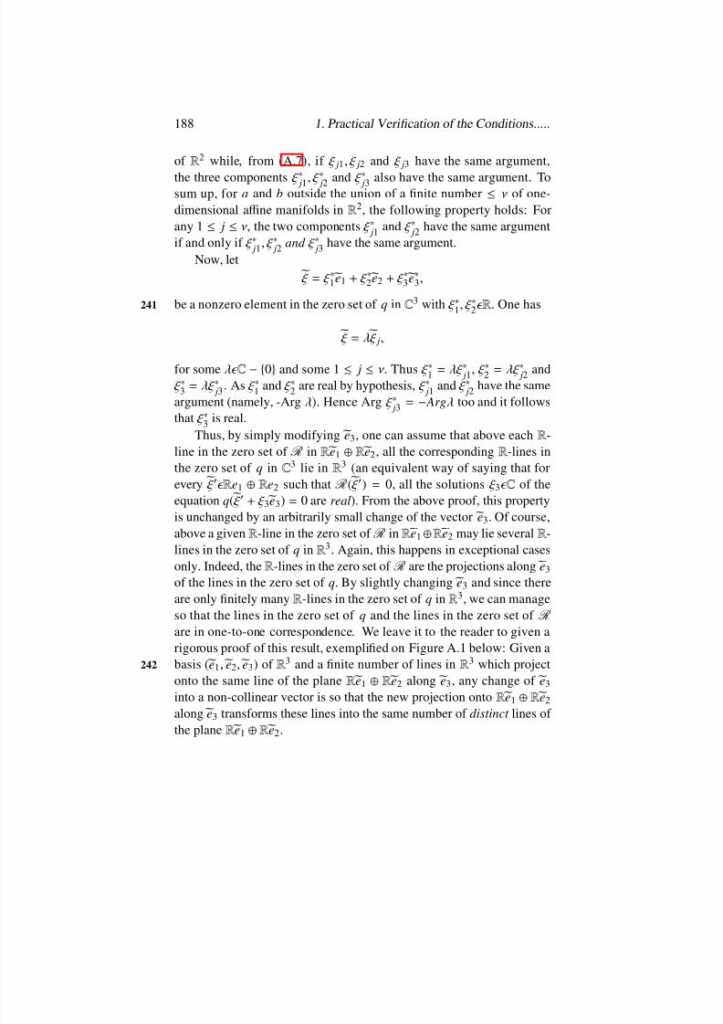
8/2/2019 Rabier-Lectures on Topics in One Parameter Bifurcation Problems
http://slidepdf.com/reader/full/rabier-lectures-on-topics-in-one-parameter-bifurcation-problems 198/238
188 1. Practical Verication of the Conditions.....
of R 2 while, from (A.7 ), if ξ j1 , ξ j2 and ξ j3 have the same argument,
the three components ξ j1 , ξ j2 and ξ j3 also have the same argument. Tosum up, for a and b outside the union of a nite number ≤ ν of one-dimensional a ffine manifolds in R 2, the following property holds: Forany 1 ≤ j ≤ν, the two components ξ j1 and ξ j2 have the same argumentif and only if ξ j1 , ξ j2 and ξ j3 have the same argument.
Now, let ξ = ξ 1e1 + ξ 2e2 + ξ 3e3 ,
be a nonzero element in the zero set of q in C 3 with ξ 1 , ξ 2 R . One has241
ξ = λ ξ j,
for some λ C − 0and some 1 ≤ j ≤ν. Thus ξ 1 = λξ j1 , ξ 2 = λξ j2 and ξ 3 = λξ j3 . As ξ 1 and ξ 2 are real by hypothesis, ξ j1 and ξ j2 have the sameargument (namely, -Arg λ). Hence Arg ξ j3 = − Arg λ too and it followsthat ξ 3 is real.
Thus, by simply modifying e3 , one can assume that above each R -line in the zero set of R in R e1 R e2 , all the corresponding R -lines inthe zero set of q in C 3 lie in R 3 (an equivalent way of saying that forevery ξ ′ R e1 R e2 such that R ( ξ ′) = 0, all the solutions ξ 3 C of theequation q( ξ ′ + ξ 3e3) = 0 are real ). From the above proof, this propertyis unchanged by an arbitrarily small change of the vector e3 . Of course,
above a given R -line in the zero set of R
in R e1 R e2 may lie several R -lines in the zero set of q in R 3 . Again, this happens in exceptional casesonly. Indeed, the R -lines in the zero set of R are the projections along e3
of the lines in the zero set of q. By slightly changing e3 and since thereare only nitely many R -lines in the zero set of q in R 3 , we can manageso that the lines in the zero set of q and the lines in the zero set of R
are in one-to-one correspondence. We leave it to the reader to given arigorous proof of this result, exemplied on Figure A.1 below: Given abasis ( e1 , e2 , e3) of R 3 and a nite number of lines in R 3 which project242
onto the same line of the plane R e1 R e2 along e3 , any change of e3
into a non-collinear vector is so that the new projection onto R e1 R e2
along e3 transforms these lines into the same number of distinct lines of the plane R e1 R e2 .
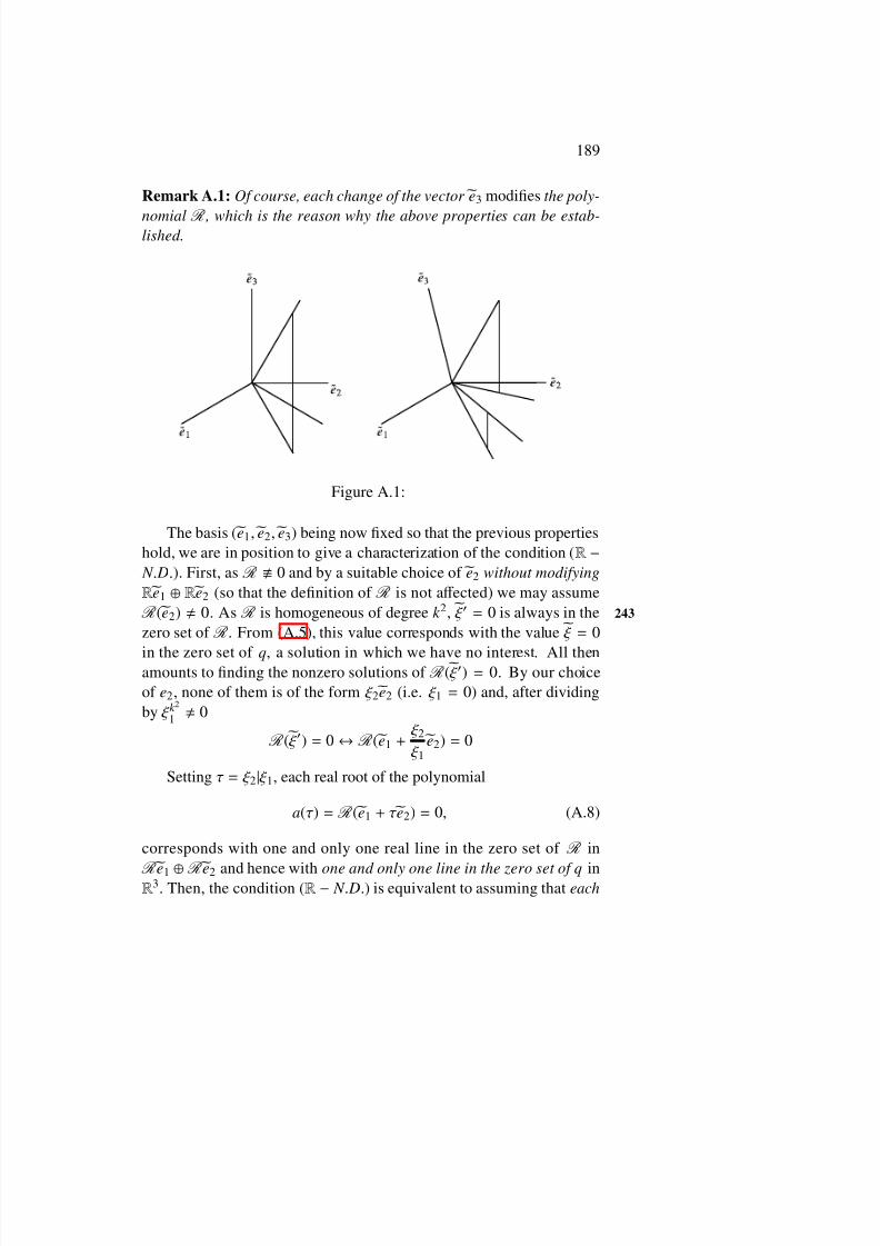
8/2/2019 Rabier-Lectures on Topics in One Parameter Bifurcation Problems
http://slidepdf.com/reader/full/rabier-lectures-on-topics-in-one-parameter-bifurcation-problems 199/238
189
Remark A.1: Of course, each change of the vector e3 modies the poly-
nomial R , which is the reason why the above properties can be estab-lished.
Figure A.1:
The basis ( e1 , e2 , e3) being now xed so that the previous propertieshold, we are in position to give a characterization of the condition ( R − N . D.). First, as R 0 and by a suitable choice of e2 without modifyingR e1 R e2 (so that the denition of R is not aff ected) we may assume R (e2) 0. As R is homogeneous of degree k 2 , ξ ′ = 0 is always in the 243
zero set of R . From (A.5) , this value corresponds with the value ξ = 0
in the zero set of q, a solution in which we have no interest. All thenamounts to nding the nonzero solutions of R ( ξ ′) = 0. By our choiceof e2 , none of them is of the form ξ 2e2 (i.e. ξ 1 = 0) and, after dividingby ξ k 2
1 0
R ( ξ ′) = 0 ↔ R (e1 +ξ 2 ξ 1
e2) = 0
Setting τ = ξ 2| ξ 1, each real root of the polynomial
a (τ ) = R (e1 + τe2) = 0, (A.8)
corresponds with one and only one real line in the zero set of R in
R e1 R e2 and hence with one and only one line in the zero set of q inR 3 . Then, the condition ( R −N . D.) is equivalent to assuming that each

8/2/2019 Rabier-Lectures on Topics in One Parameter Bifurcation Problems
http://slidepdf.com/reader/full/rabier-lectures-on-topics-in-one-parameter-bifurcation-problems 200/238
190 1. Practical Verication of the Conditions.....
real root of polynomial a (τ ) is simple . We only sketch the proof of this
result (which uses the notion of multiplicity of intersection). For thesake of brevity, we shall refer to the real zero set of q (resp. R ) as beingthe zero set of q (resp. R ) in R 3 (resp. R e1 R e2). Similar denitionswill be used for the complex zero sets of q and R .
A real line LR in the real zero set of q (resp. R ) is than the intersec-tion of one and only one complex line LC in the complex zero set of q(resp. R ) with R 3 (resp. R e1 R e2). Actually, if
LR = R ξ 0(resp .R ξ ′0 ),
then244
LC = C ξ 0(resp .C ξ ′0 ).
The line LC will be called the complex extension of LR . From ourprevious results, above the extension LC of a given line LR in the realzero set of R lines exactly one C -line in the complex zero set of q(whose intersection with R 3 is nothing but this one R -line in the realzero set of q above LR ).
To each C -line LC in the complex zero set of q is associated a multi- plicity , called the multiplicity of intersection of the surface q1 ( ξ ) = 0 andq2( ξ ) = 0 along LC . The following result is true in general (cf. [ 11 ]):The multiplicity of the root τ C of the polynomial a (τ ) (A.8 ) equals
the number of C -lines in the complex zero set of q which lie above theC -line
ξ 1e1 + τξ 1e2 , ξ 1 C,in the complex zero set of R , counted with multiplicity . On the otherhand, from the condition ( R −N . D.), the multiplicity of the complexextension of any R -line in the real zero set of q happens to be one , which,from our choice of the basis ( e1 , e2, e3 ), proves the equivalence of thecondition ( R −N . D.) with the fact that each real root of the polynomiala (τ ) (A.8) is simple.
The condition ( C − N . D.) also bears a similar characterization. Here,
the basis ( e1 , e2 , e3 ) must be taken so that the projection onto C e1 C e2of all the C -lines in the complex zero set of q are distinct. If so, the same245

8/2/2019 Rabier-Lectures on Topics in One Parameter Bifurcation Problems
http://slidepdf.com/reader/full/rabier-lectures-on-topics-in-one-parameter-bifurcation-problems 201/238

8/2/2019 Rabier-Lectures on Topics in One Parameter Bifurcation Problems
http://slidepdf.com/reader/full/rabier-lectures-on-topics-in-one-parameter-bifurcation-problems 202/238
192 1. Practical Verication of the Conditions.....
algebraic relations between the coe fficients of q which will be satised
Marsden and Schecter have suggested the use of Seidenberg’s algorithm([36 ]) to n such a system of algebraic relations characterizing the con-dition ( R − N . D.) but simplications would be desirable to get an actualpractical method of verication. Also, this approach does not yield anymeans of calculation of (approximations of) the R -lines in the zero setof q.

8/2/2019 Rabier-Lectures on Topics in One Parameter Bifurcation Problems
http://slidepdf.com/reader/full/rabier-lectures-on-topics-in-one-parameter-bifurcation-problems 203/238

8/2/2019 Rabier-Lectures on Topics in One Parameter Bifurcation Problems
http://slidepdf.com/reader/full/rabier-lectures-on-topics-in-one-parameter-bifurcation-problems 204/238
8/2/2019 Rabier-Lectures on Topics in One Parameter Bifurcation Problems
http://slidepdf.com/reader/full/rabier-lectures-on-topics-in-one-parameter-bifurcation-problems 205/238
195
It is then easy to deduce that the sequence ( M ℓ ) (respectively
( D ξ M ℓ )) tends to M (respectively D ξ M ) uniformly in the set [ −r , r ] ×C × . More precisely, introducing
w(δ) = supζ 0 C
|| A(ζ 0) − A( ξ 0 )||= | A − A( ξ 0)|∞,C , (A2.5)
one has
| M ℓ −M |∞,[−r ,r ]×C × ≤(|| A( ξ 0)||+ w(δ))|gℓ −g|∞,[−r ,r ]× (A2.6)
Besides, the same arguments leads to the inequality
| M ℓ (t ,
·,
·)
−M (t ,
·,
·)
|∞,C
×<
|| A( ξ 0)
||+ w(δ)
|gℓ (t ,
·)
−g(t ,
·)
|∞, ,
(A2.6) ′for every t [−r , r ].
Now, for ( t , ζ 0 , ξ ) [−r , r ] ×C ×
|| N ℓ (t , ζ 0 , ξ ) − N (t , ζ 0 , ξ )|| ≤2 || M ℓ (t , ζ 0 , ξ ) −M (t , ζ 0 , ξ )|||| M (t , ζ 0, ξ )||
Hence, from Lemma 2.1 of Chapter 4
| N ℓ − N |∞,[−r ,r ]×C × ≤2
1 −δ | M ℓ −M |∞,[−r ,r ]×C × , (A2.7)
from which it follows that the sequence ( N ℓ ) tends to N uniformly in the250
set [−r , r ] ×C × . The same method shows that
| N ℓ (t , ·, ·) − N (t , ·, ·)|∞,C × <2
1 −δ | M ℓ (t , ·, ·) −M (t , ·, ·)|∞,C × , (A2.7) ′
for every t [−r , r ].The proof of Theorem 5.1 of Chapter 4 is based on the following
estimate.
Lemma A2.1: For every triple (t , ζ 0 , ξ ) [−r , r ] ×C × and every ℓ N ,one has
|| D ξ N ℓ (t , ζ 0, ξ )|| ≤ 3δ(1 −δ3)
+ 2|| D ξ gℓ (0, ξ 0)||(1 −δ)w(δ)+
8/2/2019 Rabier-Lectures on Topics in One Parameter Bifurcation Problems
http://slidepdf.com/reader/full/rabier-lectures-on-topics-in-one-parameter-bifurcation-problems 206/238
196 2. Complements of Chapter IV
+ 2 || A( ξ 0)||+ w(δ)
(1 −δ)
3
(1 −δ)2 ||gℓ (t , ξ )
||+
|| D
ξ gℓ (t , ξ )
− D
ξ gℓ (0, ξ 0 )
||.
(A2.8)
Proof. In this proof, it will be convenient to use the following natation: M ℓ (resp. Λ ℓ ) will denote the value M (t , ζ 0, ξ ) (resp. D ξ M ℓ (t , ζ 0 , ξ )) at
some arbitrary point ( t , ζ 0 , ξ ) [−r , r ] ×C × and M 0ℓ (resp. Λ 0ℓ ) the par-
ticular value M ℓ (0, ξ 0 , ξ 0) (resp. D ξ mℓ (0, ξ 0 , ξ 0)). Thus, by the denitionof M ℓ
M 0ℓ = ξ 0. (A2.9)
On the other hand, the calculation of D ξ M (0, ξ 0 , ξ 0) made in Chapter
4,
§3 can be repeated for nding D
ξ M
ℓ (0, ξ
0, ξ
0) = Λ 0
ℓ so that
Λ 0ℓ h = ( ξ 0|h) ξ 0 , (A2.10)
for every h R n+ 1 . As a result
|| M 0ℓ ||= 1, (A2.11)
||Λ 0ℓ ||= 1. (A2.12)
251
With the notation introduced above, an elementary calculation gives
D ξ N ℓ (t , ζ 0 , ξ ) ·h =Λ ℓ h
|| M ℓ ||−(Λ ℓ h| M ℓ )
|| M ℓ ||3M ℓ , (A2.13)
for every h R n+ 1 . In particular, choosing ( t , ζ 0 , ξ ) = (0, ξ 0 , ξ 0), we get
D ξ N ℓ (0, ξ 0 , ξ 0) = Λ 0ℓ h −(Λ 0
ℓ h| M 0ℓ ) M 0ℓ (A2.14)
Next, from ( A2.9 )-(A2.10 ), it follows that D ξ N ℓ (0, ξ 0, ξ 0) = 0.Therefore the relation ( A2.13) is unchanged by subtracting ( A2.14 ) fromit, which means that
D ξ N ℓ (t , ζ 0 , ξ ) ·h =Λ
ℓ h
|| M ℓ ||−Λ 0ℓ h −
(Λℓ h
| M
ℓ )
|| M ℓ ||3M ℓ −(Λ 0ℓ h| M 0ℓ ) M 0ℓ

8/2/2019 Rabier-Lectures on Topics in One Parameter Bifurcation Problems
http://slidepdf.com/reader/full/rabier-lectures-on-topics-in-one-parameter-bifurcation-problems 207/238
8/2/2019 Rabier-Lectures on Topics in One Parameter Bifurcation Problems
http://slidepdf.com/reader/full/rabier-lectures-on-topics-in-one-parameter-bifurcation-problems 208/238

8/2/2019 Rabier-Lectures on Topics in One Parameter Bifurcation Problems
http://slidepdf.com/reader/full/rabier-lectures-on-topics-in-one-parameter-bifurcation-problems 209/238

8/2/2019 Rabier-Lectures on Topics in One Parameter Bifurcation Problems
http://slidepdf.com/reader/full/rabier-lectures-on-topics-in-one-parameter-bifurcation-problems 210/238

8/2/2019 Rabier-Lectures on Topics in One Parameter Bifurcation Problems
http://slidepdf.com/reader/full/rabier-lectures-on-topics-in-one-parameter-bifurcation-problems 211/238
201
compact set [ −r , r ] ×C , we may assume that r > 0 is small enough for
the inequality
|| N ℓ (t , ζ 0 , ξ 0) − N ℓ (0, ζ 0 , ξ 0)|| ≤(1 −γ )δ/ 2,
to hold for 0 ≤ℓ ≤ℓ 0 −1 and, for these indices as well, we get
|| N ℓ (t , ζ 0 , ξ ) − ξ 0|| ≤δ2
,
which completes the proof.In chapter 4, Theorem 5.1 has been used for proving the convergence
of the sequence xℓ = t ζ ℓ (where ζ ℓ + 1 = N ℓ (t , ζ 0 , ζ ℓ )) to x = t ξ (where ξ isthe unique xed point of the mapping N (t , ζ 0 ,
·) in the ball ). We shall
now give an estimate of the rate of convergence of the sequence ( xℓ ) to x under suitable assumptions on the rate of convergence of the sequence( f ℓ ) to f in appropriate spaces.
Theorem A2.1: (i) Assume that the sequence ( f ℓ ) tends to f geometri-cally in the space C k (O , R n). Then, there are constant 0 < γ ′ < 1 and K > 0 such that, for every t [−r , r ]
|| xℓ − x|| ≤K |t |γ ′ℓ , (A2.21)
for every ℓ ≥0.(ii) Assume only that the sequence
( f
ℓ )tends to f in the space C k
(O
,257
R n) , the convergence being geometrical in the space C k −1(O , R n). Then,there are constant 0 < γ ′ < 1 and K > 0 such that, for every t [−r , r ]
|| xℓ − x ≤K γ ′ℓ . (A2.22)
Proof. From the relation
ζ ℓ + 1 − ξ = N ℓ (t , ζ 0 , ζ ℓ ) − N (t , ζ 0 , ξ )
= N ℓ (t , ζ 0 , ζ ℓ ) − N ℓ (t , ζ 0 , ξ ) + N ℓ (t , ζ 0 , ξ ) − N (t , ζ 0 , ξ ),
and from Theorem 5.1 of Chapter 4, we get
||ζ ℓ + 1 − ξ ||< γ ||ζ ℓ − ξ ||+ || N ℓ (t , ζ 0 , ξ ) − N (t , ζ 0 , ξ )||.
8/2/2019 Rabier-Lectures on Topics in One Parameter Bifurcation Problems
http://slidepdf.com/reader/full/rabier-lectures-on-topics-in-one-parameter-bifurcation-problems 212/238

8/2/2019 Rabier-Lectures on Topics in One Parameter Bifurcation Problems
http://slidepdf.com/reader/full/rabier-lectures-on-topics-in-one-parameter-bifurcation-problems 213/238
203
To prove (ii), we use the same method, replacing the relations ( A2.6 )
and (A2.7 ) by (A2.6) ′ and (A2.7) ′. With ( A2.23 ), we get
||ζ ℓ + 1 − ξ || ≤γ ||ζ ℓ − ξ ||+2(|| A( ξ 0 )||+ w(δ))
1 −δ |gℓ (t , ·) −g(t , ·)|∞, .
Now, note that
|gℓ (t , ·) −g(t , ·)|∞, ≤k
|t |1 +
δ2
k −1
| Dk −1 ( f ℓ − f )|∞,O .
Indeed, this is obvious if k = 1. If k ≥2, the inequality follows fromthe relation
gℓ (t , ζ ) −g(t , ζ ) =k (k −1)
t 1
0(1 −s)k −1 Dk −1( f ℓ − f )( st ζ ) ·(ζ )k −1ds .
Arguing as before, we nd the analogue of ( A2.24 ), namely 259
||ζ ℓ − ξ || ≤γ ℓ 1 +ℓ C γ |t |
,
for every ℓ ≥0. Multiplying by |t | > 0, we obtain
|| xℓ − x|| ≤γ ℓ |t |+
ℓ C γ ≤γ ℓ r +
ℓ C γ
.
Choosing γ < γ ′ < 1, the inequality ( A2.22) follows with
K = supℓ ≥0
γ γ ′
ℓ
r +ℓ C γ
< +∞,
and remains valide for t = 0.
We shall now prove the results about convergence in the spaces of type C k that we used in §6 of Chapter 4. Recall that given a real Banachspace Z and a mapping Φ (= Φ ( x, z)) C k (O ×B(0, ρ), Z ), k ≥1, where
B(0, ρ) denotes the closed ball with radius ρ > 0 centered at the origin of Z , verifying Φ (0) = 0 and D zΦ (0) = 0, it is possible to shrink ρ > 0 and

8/2/2019 Rabier-Lectures on Topics in One Parameter Bifurcation Problems
http://slidepdf.com/reader/full/rabier-lectures-on-topics-in-one-parameter-bifurcation-problems 214/238
204 2. Complements of Chapter IV
the neighbourhood O so that, given any arbitrary constant 0 < β < 1,
one has|| D zΦ ( x, z)|| ≤β (A2.25)
for every ( x, z) O × B(0, ρ) and the mapping Φ ( x, ·) is a contraction withconstant β from B(0, ρ) to itself for every x O . If so, for x O , the se-quence
0( x) = 0,
ℓ + 1( x) = Φ ( x, ℓ ( x)), ℓ ≥0,
is well dened, each mapping ℓ being in the space C k (O , Z ) with valuesin B(0, ρ). We already know that this sequence converges pointwise to260
the mapping C k
(O
, Z ) characterized by( x) = Φ ( x, ( x)),
for every x O . In §6 of Chapter 4, we used the fact that the sequence( ℓ ) tends to in the space C k (O , Z ), the convergence being geometricalin the space C k −1(O , Z ). Proving this assertion will take us a certainamount of time. To begin with, we show that
Lemma A2.2: The sequence ( ℓ ) tends to in the space C 0(O , Z ).
Proof. Let ℓ ≥1 be xed. For every x O
ℓ + 1( x) − ℓ ( x) = Φ ( x, ℓ ( x)) −Φ ( x, ℓ −1( x))
= 10 D zΦ ( x, ℓ −1( x) + s( ℓ ( x) − ℓ −1( x)))·
( ℓ ( x) − ℓ −1( x))ds .
Due to ( A2.25 ) we obtain
|| ℓ + 1( x) − ℓ ( x)|| ≤β|| ℓ ( x) − ℓ −1( x)||,for every x O . Thus
| ℓ + 1 − ℓ |∞,O ≤β| ℓ − ℓ −1|∞,O .

8/2/2019 Rabier-Lectures on Topics in One Parameter Bifurcation Problems
http://slidepdf.com/reader/full/rabier-lectures-on-topics-in-one-parameter-bifurcation-problems 215/238
205
Hence, the sequence ( ℓ ) tends (geometrically) to a limit in the space
C 0(O , Z ). Of course, this limit must be the pointwise limit and the
proof is complete.For j ≥0, let us denote by L j(R n+ 1 , Z ) the space of j-linear map-
pings from R n+ 1 into Z with the usual abuse of notation L 0(R n+ 1 , Z ) = Z . Also, recall the canonical isomorphism
L i+ 1 (R n+ 1 , Z ) L (R n+ 1 , L i(R n+ 1 , Z )), (A2.26)
which will be repeatedly used in sequel. 261
We shall denote by λ i the generic element of the space L i(R n+ 1 , Z ).Due to the identication L 0(R n+ 1 , Z ) = Z , this means, in particular,
that we shall identify the element z Z with λ0 so that the assumption D xΦ (0) = 0 will be rewritten as
Dλ0 Φ (0) = 0. (A2.27)
Now, setting Φ = Φ 0 , introduce the mappings
Φ j : O ×B(0, ρ) × j
i= 1
L i(R n+ 1 , Z ) →L j(R n+ 1 , Z ), 1 ≤ j ≤k ,
by
Φ j( x, λ 0 , · · ·, λ j) = ∂Φ j−1∂ x
( x, λ 0 , · · ·, λ j−1) + (A2.28)
+ j−1
i= 0
∂Φ j−1
∂λ i( x, λ 0, · · ·, λ j−1 )λ i+ 1 ,
where the term∂Φ j−1
∂λ i( x, λ 0 , · · ·, λ j−1)λ i+ 1 is the product of the linear
mappings
∂Φ j−1
∂λ i( x, λ 0, · · ·, λ j−1 ) L (L i(R n+ 1, Z ), L j−1 (R n+ 1 , Z ))
and λ i+ 1 L (R n , L i(R n+ 1 , Z )).

8/2/2019 Rabier-Lectures on Topics in One Parameter Bifurcation Problems
http://slidepdf.com/reader/full/rabier-lectures-on-topics-in-one-parameter-bifurcation-problems 216/238
206 2. Complements of Chapter IV
Remark A2.1: Observe, in particular, that the only term involving λ j in
the denition of Φ j, j ≥1 , is the term∂Φ
j−1∂λ j−1 ( Z , λ 0 , · · ·, λ j−1)λ j it followsthat Φ j( x, λ 0 , · · ·, λ j) is linear with respect to λ j when j ≥1.
The importance of the mappings Φ j, 0 ≤ j ≤k lies in the fact that
D j ( x) = Φ j( x, ( x), D ( x), · · ·, D j ( x)), 0 ≤ j ≤k (A2.29)
for every x O and, for every ℓ ≥0262
D jℓ + 1( x) = Φ j( x, ℓ ( x), D ℓ ( x), · · ·, D j
ℓ ( x)), 0 ≤ j ≤k , (A2.30)
for every x O . These properties can be immediately checked by in-duction. Also, it is clear that the mapping Φ j is of class C k − j and, for
1 ≤ j ≤ k , Φ j is of class C ∞ with respect to ( λ1 , · · ·, λ j). We nowestablish two simple preliminary lemmas.
Lemma A2.3: Given any index 0 ≤ j ≤k, one has
∂Φ j
∂λ j(0, 0, λ 1 , · · ·, λ j) = 0, (A2.31)
for every (λ1 , · · ·, λ j) j
i= 1L i(R n+ 1 , Z ).
Proof. For j = 0, the result is nothing but ( A2.27 ). For j ≥1, it followsfrom Remark A2.1 that for every µ j L (R n+ 1 , Z )
∂Φ j
∂λ j( x, λ 0 , · · ·, λ j) · µ j =
∂Φ j−1
∂λ j−1( x, λ 0 , · · ·, λ j−1 ) µ j.
Choosing x = 0, λ 0 = 0, the above relation yields the desired resultby an indeuction argument.
Lemma A2.4 : Let the index 0 ≤ j ≤ k be xed. If the sequence ( ℓ )tends to in the space C j(O , Z ) (which is already known for j = 0), theset
Λ j =ℓ ≥0
D jℓ (O ) L j(R n+ 1 , Z ), (A2.32)
is compact and one has D j (O ) Λ j. (A2.33)
8/2/2019 Rabier-Lectures on Topics in One Parameter Bifurcation Problems
http://slidepdf.com/reader/full/rabier-lectures-on-topics-in-one-parameter-bifurcation-problems 217/238
207
Proof. A sequence in the setℓ
≥0 D j
ℓ (O ) is of the form ( λ ( p) j ) p> 0 where263
for each p N there is an index ℓ = ℓ ( p) and an element x p O suchthat λ ( p)
j = D jℓ ( p)( x p). If, for innitely many indices p, namely for a
subsequence ( pm), the index ℓ ( pm) equals some xed value ℓ , one has
λ ( pm ) j = D j
ℓ ( x pm ).
As the set O is compact and after extracting a subsequence, we mayassume that there is x O such that the sequence ( x pm ) tends to x. Bycontinuity of the mapping D j
ℓ , we deduce that the sequence λ ( pm) j tends
to D jℓ ( x) as m tends to + ∞.
Now, assume that the mapping p
→ℓ ( p) takes only nitely many
times any given value ℓ . Then, there is a subsequence ℓ ( pm) which isstrictly increasing and thus tends to +∞as m tends to + ∞. For every m,let us write
D jℓ ( pm)( x pm ) = D j
ℓ ( pm)( x pm ) − D j ( x pm ) + D j ( x pm ).
Again, in view of the compactness of the set O , we may assumethat the sequence ( x pm ) tends to x O . As the sequence ( D j
ℓ )ℓ ≥0 tendsto D j in the space C 0(O , L j(R n+ 1 , Z )), by hypothesis, the same prop-erty holds for the subsequence ( D j
ℓ ( pm))m≥0 . Therefore, in the spaceL j(R n+ 1, Z )
limm→+ ∞ D j ℓ ( pm)( x pm ) − D j ( x pm ) = 0
On the other hand, by the continuity of the mapping D j , we get
limm→+ ∞
D j ( x pm ) = D j ( x).
264
As a result, the sequence ( λ ( pm) j )m≥0 tends to D j ( x).
To sum up, we have shown that every sequence ( λ ( p) j ) p≥0 of the set
ℓ ≥0 D j
ℓ (O ) has a cluster point in the space L j(R n+ 1 , Z ) and hence is
relatively compact, which proves ( A2.32 ). The relation ( A2.33) is now
obvious since D j
( x) is the limit of the sequence ( D j
ℓ ( x))ℓ ≥0 for every x O .

8/2/2019 Rabier-Lectures on Topics in One Parameter Bifurcation Problems
http://slidepdf.com/reader/full/rabier-lectures-on-topics-in-one-parameter-bifurcation-problems 218/238
8/2/2019 Rabier-Lectures on Topics in One Parameter Bifurcation Problems
http://slidepdf.com/reader/full/rabier-lectures-on-topics-in-one-parameter-bifurcation-problems 219/238

8/2/2019 Rabier-Lectures on Topics in One Parameter Bifurcation Problems
http://slidepdf.com/reader/full/rabier-lectures-on-topics-in-one-parameter-bifurcation-problems 220/238

8/2/2019 Rabier-Lectures on Topics in One Parameter Bifurcation Problems
http://slidepdf.com/reader/full/rabier-lectures-on-topics-in-one-parameter-bifurcation-problems 221/238
8/2/2019 Rabier-Lectures on Topics in One Parameter Bifurcation Problems
http://slidepdf.com/reader/full/rabier-lectures-on-topics-in-one-parameter-bifurcation-problems 222/238

8/2/2019 Rabier-Lectures on Topics in One Parameter Bifurcation Problems
http://slidepdf.com/reader/full/rabier-lectures-on-topics-in-one-parameter-bifurcation-problems 223/238
213
+ j−1
i= 0 || B j−1
iℓ ( x)
−B j−1
i( x)
|||| Di+ 1 ( x)
||(A2.46)
+ j−1
i= 0|| B
j−1iℓ ( x)|||| D
i+ 1ℓ ( x) − Di+ 1 ( x)||.
It is essential to pay special attention to the term corresponding withi = j −1 in the last sum, namely || B
j−1 j−1,ℓ ( x)|||| D j
ℓ ( x) −D j ( x)||. From(A2.39 )
B j−1 j−1,ℓ ( x) =
∂Φ j−1
∂λ j−1( x, ℓ ( x), D ℓ ( x), · · ·, D j−1
ℓ ( x)).
As the sequence ( ℓ ) tends to in the space C j−1(O , Z ) by hypoth-esis, we can apply Lemma A2.5 with j −1 (which amount to shrinkingthe neighbourhood O if necessary) and hence
|| B j−1 j−1,ℓ ( x)|| ≤β,
for every x O . Inequality (A2.46 ) becomes
|| D j
ℓ + 1( x) − D j ( x)||< ||b j−1ℓ ( x) −b j−1 ( x)||
+ j−1
i= 0 || B j−1
iℓ ( x)
−B j−1
i( x)
−B j−1
i( x)
|||| Di+ 1
||(A2.47)
+ j−2
i= 0|| B
j−1iℓ ( x)|||| D
i+ 1ℓ ( x) − Di+ 1 x||+
+ β|| D j
ℓ − D j ( x)||.Now, since j ≤ k −1, we can apply Lemma A2.6 (i) with j −1: 271
There are constant q with 0 < q < 1 and C > 0 such that
||b j−1
ℓ ( x)
−b j−1( x)
|| ≤Cq ℓ ,
|| B j−1iℓ ( x) −B j−1
i ( x)|| ≤Cq ℓ , 0 ≤i ≤ j −1,

8/2/2019 Rabier-Lectures on Topics in One Parameter Bifurcation Problems
http://slidepdf.com/reader/full/rabier-lectures-on-topics-in-one-parameter-bifurcation-problems 224/238

8/2/2019 Rabier-Lectures on Topics in One Parameter Bifurcation Problems
http://slidepdf.com/reader/full/rabier-lectures-on-topics-in-one-parameter-bifurcation-problems 225/238

8/2/2019 Rabier-Lectures on Topics in One Parameter Bifurcation Problems
http://slidepdf.com/reader/full/rabier-lectures-on-topics-in-one-parameter-bifurcation-problems 226/238
8/2/2019 Rabier-Lectures on Topics in One Parameter Bifurcation Problems
http://slidepdf.com/reader/full/rabier-lectures-on-topics-in-one-parameter-bifurcation-problems 227/238
8/2/2019 Rabier-Lectures on Topics in One Parameter Bifurcation Problems
http://slidepdf.com/reader/full/rabier-lectures-on-topics-in-one-parameter-bifurcation-problems 228/238
8/2/2019 Rabier-Lectures on Topics in One Parameter Bifurcation Problems
http://slidepdf.com/reader/full/rabier-lectures-on-topics-in-one-parameter-bifurcation-problems 229/238

8/2/2019 Rabier-Lectures on Topics in One Parameter Bifurcation Problems
http://slidepdf.com/reader/full/rabier-lectures-on-topics-in-one-parameter-bifurcation-problems 230/238
8/2/2019 Rabier-Lectures on Topics in One Parameter Bifurcation Problems
http://slidepdf.com/reader/full/rabier-lectures-on-topics-in-one-parameter-bifurcation-problems 231/238
221
Lemma A2.8: (i) Assume k ≥2 and 0 ≤ j ≤k −2. Then, the sequence279
(c jℓ )ℓ ≥0 tends to c
jgeometrically in the space C
0(O , L (R
n+ 1, L j(R
n+ 1,
R n))) and the sequence (C jiℓ )ℓ ≥0 tends to C ji in the space C 0(O ,L (L i(R n+ 1 , R n) , L j(R n+ 1 , R n))) .
(ii) Assume only k ≥1 and 0 ≤ j ≤k −1. Then, the sequence (c jℓ )ℓ ≥0
tends to c j in the space C 0(O , L (R n+ 1 , L j(R n+ 1 , R n))) and the sequence(C jiℓ )ℓ ≥0 tends to C j
i in the space C 0(O , L (L i(R n+ 1 , R n), L i(R n+ 1 , R n))) .
Proof. The proof of this lemma parallels that of Lemma A2.6 . Noteonly that the (geometrical) convergence of the sequence ( ℓ + k ) to inthe space C j(O , Z ) need not be listed in the assumption since it is knownfrom Theorem A2.2
Theorem A2.4 : The sequence ( f ℓ ) tends to f in the space C k (O , R n)and the convergence is geometrical in the space C k −1 (O , R n).
Proof. Once again, it is enough to prove equivalently that the sequence( D j f ℓ )ℓ ≥0 tends to D j f in the space C 0(O , L j(R n+ 1 , R n)) for 0 ≤ j ≤k , the convergence being geometrical for 0 ≤ j ≤ k −1. We shalldistinguish the case j = 0 and j ≥1.
When j = 0, we must prove that the sequence ( f ℓ ) tends to f ge-ometrically in the space C 0(O , R n). By denition and with the Taylorformula (since F is at least C 1), one has for x O and ℓ ≥0
f ℓ ( x) −f ( x)=
F ( x, ℓ + k ( x)) −F ( x, ( x))= 1
0
∂F ∂λ 0
( x, ( x) + s( ℓ + k ( x) − ( x))) ·( ℓ + k ( x) − ( x))ds .
By the continuity of the mapping ( ∂F /∂λ 0) on the compact set O × 280Λ c
0, where Λ c0 B(0, ρ) denotes the closed convex hull of the compact
set Λ 0 (cf. Lemma A2.4 ), there is a constant K > 0 such that
||∂F ∂Λ 0
( x, ( x) + s( ℓ + k ( x) − ( x)))|| ≤K ,
for every x O and ℓ
≥0. Hence
| f ℓ − f |∞,O ≤K | ℓ + k − |∞,O

8/2/2019 Rabier-Lectures on Topics in One Parameter Bifurcation Problems
http://slidepdf.com/reader/full/rabier-lectures-on-topics-in-one-parameter-bifurcation-problems 232/238
222 2. Complements of Chapter IV
and the geometrical rate o ff convergence of the sequence ( f ℓ ) to f in the
space C 0(O , R
n) follows from Theorem A2.2 .
When 1 ≤ j ≤ k and with ( A2.60 ) - (A2.62) and the notation(A2.63 )-(A2.66 ), the method we used in Theorem A2.2 and A2.3 leadsto the inequality
|| D j f ℓ ( x) − D j f ( x)|| ≤ ||c j−1
ℓ ( x) −C j−1( x)||+ ||
j−1
i= 0||c
j−1iℓ ( x) − ||C j−1
i ( x)|||| Di+ 1|| ( x)||
+ j−1
i= 0||C j−1
iℓ ( x)|||||| Di+ 1ℓ + k ( x) − || Di+ 1 ( x)||,
for every x O . Due to the compactness of the set O ×Λ 0 × · · · ×Λ j−1
(Lemma A2.4) and the regularity C k (O , Z ), there is a constant K > 0such that
|| Di+ 1 ( x)|| ≤K ,
||C −ıℓ j−1 ( x)|| ≤K ,
for x O , 0 ≤i ≤ j −1 and ℓ ≥0. Thus, we rst obtain
|| D j f ℓ ( x) − D j f ( x)||< ||c
j−1ℓ ( x) −c j−1( x)
+ K j−1
i= 0||C j−1
iℓ ( x) −C j−1i ( x)||+ || Di+ 1
ℓ + k ( x) − Di+ 1 ( x)||and next281
| D j( f ℓ −f )|∞,O ≤ |c jℓ −c j−1|∞,O
+ K | j−1
i= 0|C j−1
iℓ −C j−1i |∞,O + Di+ 1( ℓ + k − )|∞,|O .
(A2.67)
For k ≥2 and 1 ≤ j ≤k −1 (i.e. 0 ≤ j −1 ≤k −2). this inequalityyields the geometrical convergence of the sequence ( D j f ℓ )ℓ ≥0 to D j f in
8/2/2019 Rabier-Lectures on Topics in One Parameter Bifurcation Problems
http://slidepdf.com/reader/full/rabier-lectures-on-topics-in-one-parameter-bifurcation-problems 233/238

8/2/2019 Rabier-Lectures on Topics in One Parameter Bifurcation Problems
http://slidepdf.com/reader/full/rabier-lectures-on-topics-in-one-parameter-bifurcation-problems 234/238
8/2/2019 Rabier-Lectures on Topics in One Parameter Bifurcation Problems
http://slidepdf.com/reader/full/rabier-lectures-on-topics-in-one-parameter-bifurcation-problems 235/238
8/2/2019 Rabier-Lectures on Topics in One Parameter Bifurcation Problems
http://slidepdf.com/reader/full/rabier-lectures-on-topics-in-one-parameter-bifurcation-problems 236/238
8/2/2019 Rabier-Lectures on Topics in One Parameter Bifurcation Problems
http://slidepdf.com/reader/full/rabier-lectures-on-topics-in-one-parameter-bifurcation-problems 237/238
BIBLIOGRAPHY 227
Anderson Ed. Ann. of Math. Studies, 69, Princerton University
Press (1972).[22] LUUSTERNIK, L.A. - SOBOLEV, V.J. : E lements of Functional
Analysis, Gordon and Breach (1961).
[23] Mc LEOD, J.B.-SATTINGER, D. : Loss of Stability and Bifurca- 284
tion at Double Eigenvalues, J . Funct, Anal., 14, 62-84 (1973).
[24] MAGNUS, R.J. : On the Local Structure of the Zero Set of a Ba-nach Space Valued Mapping, J . Funct. Anal., 22, 58-72 (1976).
[25] MARSDEN, J. : Qualitative Methods in Bifurcation Theory, Bull.Amer. Math. Soc., 84, 1125-1148 (1978).
[26] MUMFORD, D. : Algebraic Geometry I. Complex Projective Va-rieties, Frundlehren der Math. Wiss., 221, Springer (1976).
[27] NIRENBERG, L. : T opics in Nonlinear Functional Analysis,Courant Institute Lecture Notes (1974).
[28] PALAIS, R. : The Morse Lemma on Banach Spaces, Bull. Amer.Math Soc.,75, 968-971 (1969).
[29] RABIER, P. : A Generalization of the Implicit Function Theoremfor Mappings from R n+ 1 into R n and its Applications, J . Funct.Anal., 56, 145-170 (1984).
[30] RABIER, P. : A Necessary and Su fficient Condition for the Co-erciveness of Certain Functionsl, STAM J. MAth. Anal., Vol. 15,no.2, 367-388 (1984).
[31] RABIER, P. : A Synthetic Study of One-Parameter NonlinearProblems (Preprint).
[32] RABIER, P. : A Desingularization Process in Degenerate Bifurca-tion Problems, Parts I and II (Preprint).
[33] RABIER, P.-EL HAJJI, S. : New Algorithms for the Computation 285
of the Branches in One-Parameter Nonlinear Problems (To appearin N um. Mat.).

8/2/2019 Rabier-Lectures on Topics in One Parameter Bifurcation Problems
http://slidepdf.com/reader/full/rabier-lectures-on-topics-in-one-parameter-bifurcation-problems 238/238