Multipath Mitigation for Bridge Deformation Monitoring - Scientific

Marine and Freshwater Resources Institute
Integrated Scientific Monitoring ProgramDevelopment of a “design model” for an
adaptive ISMP sampling regime
Final report to theAustralian Fisheries Management Authority
December 2001
Ian Knuckey& Anne Gason
ARF Project R99/1502

Marine and Freshwater Resources Institute
Integrated Scientific Monitoring ProgramDevelopment of a “design model” for an
adaptive ISMP sampling regime
Final report to theAustralian Fisheries Management Authority
December 2001
Ian Knuckey& Anne Gason
ARF Project R99/1502
Marine and Freshwater Resources InstitutePO Box 114
Queenscliff VIC 3225

Marine and Freshwater Resources Institute
ARF Project R99/1502 Final Report - Page i
© The State of Victoria, Department of Natural Resources and Environment, 2001
This work is copyright. Apart from any use under the Copyright Act 1968, nopart may be reproduced by any process without written permission.
ISBN: 1 74106 400 7
Copies available from:LibrarianMarine and Freshwater Resources InstitutePO Box 114Queenscliff VIC 3225
Phone: (03) 5258 0259Fax: (03) 5258 0270Email: [email protected]
Preferred way to cite this publication:Knuckey, I A and Gason, A. (2001). Development of a “design model” for anadaptive ISMP sampling regime. ARF Project R99/1502. Final report to theAustralian Fisheries Management Authority. 70pp. (Marine and FreshwaterResources Institute: Queenscliff).
General disclaimer:This publication may be of assistance to you but the State of Victoria and itsemployees do not guarantee that the publication is without flaw of any kind or iswholly appropriate for your particular purposes and therefore disclaims allliability for any error, loss or other consequence which may arise from you relyingon any information in this publication.

Marine and Freshwater Resources Institute
ARF Project R99/1502 Final Report - Page ii
Table of ContentsNON-TECHNICAL SUMMARY .........................................................................................1
BACKGROUND....................................................................................................................3
OBJECTIVES ........................................................................................................................5
METHODS ............................................................................................................................5
Data inputs ..........................................................................................................................5
Stratification........................................................................................................................8
Simulation modelling and estimation of discard rates and corresponding CVs. ................8
Sampling for length and age .............................................................................................10
RESULTS & DISCUSSION................................................................................................12
Data inputs ........................................................................................................................12
Stratification......................................................................................................................12
Simulation modeling and estimation of discard rates and corresponding CVs ................16
Sampling for length and age .............................................................................................18
Implications of the design model for an adaptive ISMP sampling regime.......................18
References ............................................................................................................................21
Tables ...................................................................................................................................22
Figures..................................................................................................................................30
Marine and Freshwater Resources Institute
ARF Project R99/1502 Final Report - Page 1
NON-TECHNICAL SUMMARY
R99/1502 Development of a “design model” for an adaptive ISMP sampling regime.
Principal investigator: Ian Knuckey
Co-investigator: Anne Gason
Address: Marine and Freshwater Resources Institute
P.O. Box 114
Queenscliff, VIC 3225
OBJECTIVES:
1. To develop a "design model" for updating the ISMP sampling regime to reflect the most
recent data available from the trawl and non-trawl sectors of the SEF.
2. To provide a statistically sound basis for maintaining a cost-effective sampling regime for
estimating the total catch (retained and discarded) and length/age composition of quota
species and other species caught by the trawl and non-trawl sectors of the SEF.
Non-Technical Summary
The South East Fishery (SEF) is a commonwealth-managed multi-species fishery comprising
of both trawl and non-trawl vessels working in the waters off south eastern Australia. The
Integrated Scientific Monitoring Program (ISMP) was established in 1994 to provide essential
information on the species composition of the retained and discarded catch from the SEF and
the size and age composition of selected quota and non-quota species.
Over the last three years, the original ISMP sampling design (Smith et al. 1997) has proven to
be statistically robust, meeting virtually all of the target CVs for estimates of discard rates and
length frequency distributions for all species (Knuckey and Sporcic 1999, Knuckey 2000,
Knuckey et al. 2001). In each of these reports, however, it was noted that there were cases in
which target sea-days for a particular strata were not achieved because of significant changes
in the fleet dynamics of the fishery when compared to the data on which the ISMP design was
originally based.
Due to changes in fleet dynamics, patterns of discarding, the addition of new strata in the
trawl sector as well as the availability of data for the non-trawl sector, it became apparent that

Marine and Freshwater Resources Institute
ARF Project R99/1502 Final Report - Page 2
there was a pressing need to review the ISMP sampling regime so that it was better able to
reflect the dynamics of the fishery and include monitoring of the non-trawl fishery. It was
recognised that in a complex and dynamic fishery such as the SEF, any revision would need
to be undertaken on a regular basis to ensure that the monitoring program adequately sampled
fishery, yet the ongoing process needed to be relatively automated to minimise the costs
involved. The present study has addressed this need by developing an ‘adaptive survey
design strategy’ that utilises past information as well as the most recent logbook and ISMP
data to revise the ISMP sampling strategy on an annual basis.
A Bayesian framework was used to incorporate prior information and then apply these priors
to update the sampling design, thereby providing a basis for adjusting the intensity and spatial
distribution of the sampling to meet the level of precision required for the management needs
of SEFAG, SETMAC and AFMA and for input into agreed stock assessment models.

Marine and Freshwater Resources Institute
ARF Project R99/1502 Final Report - Page 3
BACKGROUNDThe South East Fishery (SEF) is a commonwealth-managed multi-species fishery comprising
of both trawl and non-trawl vessels working in the waters off south eastern Australia. The
Australian Fisheries Management Authority has collected catch and effort logbook data
(SEF1) since 1986 and, when quota controls were introduced in 1992, quota monitoring data
also became available. The Integrated Scientific Monitoring Program (ISMP) was established
in 1994 to augment these data with essential information on the species composition of the
retained and discarded catch and the size and age composition of selected quota and non-
quota species. To achieve this, the ISMP has two main data collection components: at-sea
monitoring of the composition of trawl catches by on-board field scientists; and port-based
collection of length frequency information on the landed catches of both trawl and non-trawl
vessels.
The objective of the current ISMP sampling regime, designed by Smith et al. (1997), was to
provide estimates (within specified error bounds) of the total catch (retained and discarded) of
quota and non-quota species and the size and age composition of selected quota species. To
enable this, the fishery was characterised using quota monitoring and logbook information
from 1992 to 1996 inclusive, together with data from the ISMP’s predecessor, the Scientific
Monitoring Program. These extensive data sets provided the spatial and temporal information
that allowed stratification of the fishery based on species composition, fishing methods and
port groups. Three species-specific target fisheries were recognised (orange roughy,
spawning blue grenadier and royal red prawn) but sections of the fishery targeting a mixed
species catch were more difficult to categorise and required grouping into “inshore” and
“offshore” (equivalent to shelf and slope) reflecting the difference in species assemblages
with depth. A further factor considered was the size of vessel landings (high volume and low
volume). Overall, 14 strata were defined (Table 1). The amount of sampling required in each
stratum reflected the species composition and the relative discard rates (% of catch discarded)
of these species. Significant emphasis was given to the estimation of discard rates, as this is
typically the most difficult and expensive component of such a program. Species were
grouped by discard rate into three groups: low (<5%), moderate (5–20%), and high (>20%)
for which the target coefficients of variation (CVs) were 1.5, 0.8 and 0.4 respectively.
Simulation modelling was used to determine the number of trips required in each stratum to
achieve these targets. Further, to account for seasonal variation in fishing effort, the annual
number of trips per stratum were divided into months based on the monthly proportion of
commercial fishing shots per stratum recorded in the SEF1 and SEF2 databases.

Marine and Freshwater Resources Institute
ARF Project R99/1502 Final Report - Page 4
Over the last three years, the ISMP sampling design has proven to be statistically robust,
meeting virtually all of the target CVs for estimates of discard rates and length frequency
distributions for all species (Knuckey and Sporcic 1999, Knuckey 2000, Knuckey et al.
2001). In each of these reports, however, it was noted that there were cases in which target
sea-days for a particular strata were not achieved because of significant changes in the fleet
dynamics of the fishery when compared to the data on which the ISMP design was originally
based. For example, the original sampling design did not reflect the increasing proportion of
southern NSW and Lakes Entrance/Eden vessels that now move south to fish off eastern
Tasmania over the summer period. Also, in the initial design there was both inshore and
offshore strata for the Lakes Entrance/Eden vessels and these vessels often fished either one
or the other in any given trip but current ISMP and SEF1 data indicated that vessels now often
fished both strata within the one trip. Furthermore, patterns of discarding of many species
have changed over time to an extent where the original discard classification (and target CVs)
were no longer applicable.
Another issue was that when the ISMP sampling regime was designed, there was no on-board
monitoring information available on the non-trawl sector. As such, the non-trawl sector could
not be included as a statistically valid stratum within the design. To rectify this, a pilot
monitoring program was undertaken during 1999/2000 to monitor the amount and
composition of the retained and discarded catches of SEF non-trawl vessels. This program
has now been completed and the data has been analysed (Knuckey et al. 2001a) so that on-
board monitoring of non-trawl vessels can now be incorporated into a “unified” ISMP
sampling design.
Overall, it was apparent that there was a pressing need to review the ISMP sampling regime
so that it was better able to reflect the dynamics of the fishery and include monitoring of the
non-trawl fishery. It was recognised that in a complex and dynamic fishery such as the SEF,
any revision would need to be undertaken on a regular basis to ensure that the monitoring
program adequately sampled fishery, yet the ongoing process needed to be relatively
automated to minimise the costs involved. The present study has addressed this need by
developing an ‘adaptive survey design strategy’ that utilises past information as well as the
most recent logbook and ISMP data to revise the ISMP sampling strategy on an annual basis.
A Bayesian framework was used to incorporate prior information and then apply these priors
to update the sampling design, thereby providing a basis for adjusting the intensity and spatial
distribution of the sampling to meet the level of precision required for the management needs
of SEFAG, SETMAC and AFMA and for input into agreed stock assessment models.

Marine and Freshwater Resources Institute
ARF Project R99/1502 Final Report - Page 5
OBJECTIVES1. To develop a "design model" for updating the ISMP sampling regime to reflect the most
recent data available from the trawl and non-trawl sectors of the SEF.
2. To provide a statistically sound basis for maintaining a cost-effective sampling regime for
estimating the total catch (retained and discarded) and length/age composition of quota
species and other species caught by the trawl and non-trawl sectors of the SEF.
METHODSData inputs
The data used to develop the ‘design model’ included: catch and effort logbook information
from the trawl sector (SEF1) and non-trawl sector (GN01 and GN01a); catch landings
information for quota species (SEF2), on-board scientific observer monitoring of trawl fishing
during the 7-year period 1993-2000; on-board scientific observer monitoring of non-trawl
fishing during the 15 months March 1999-May 2000; and port-based measuring for both
sectors. Details of these datasets are provided below.
SEF1 and GN01(a)
These data were obtained from compulsory logbooks filled out by the skipper of each vessel
permitted to operate in the SEF. The data were stored on the Australian Fishing Zone
Information System (AFZIS), an INGRES relational database. SEF1 data were obtained for
the period 1993 to 2000 and GN01(a) data were obtained from 1998 to 2000. The
information used from each logbook record included:
Boatname
Date
Operation (shot) number
Fishing method
Fishing activity
Start position (latitude and longitude)
End position (latitude and longitude)
Species name
Estimated weight of species caught
SEF2
The SEF2 data, also stored on AFZIS, were used by AFMA to monitor the catch of species
against their TAC’s. The data were obtained from fishers at the end of each fishing trip.
Marine and Freshwater Resources Institute
ARF Project R99/1502 Final Report - Page 6
SEF2 data for the period 1992 to 2000 were used. The information used from each SEF2
record included:
Boatname
Date
Port landed
Processor
Transport company
Species name
Weight of species caught
On board monitoring (trawl and non-trawl)
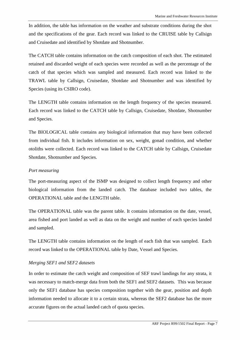
The trawl data collected by the on-board observers with the ISMP (and its predecessor, the
SMP) were extremely detailed. They were stored in a relational database comprised of six
tables as shown below. These ISMP data from trawlers were used for the period 1993 to 2000.
The on-board data for the non-trawl vessels was very similar to that of the ISMP but it was
only collected from the Pilot Non-trawl Monitoring Program that ran from March 1999 to
May 2000.
The CRUISE table was the parent table to which all other tables refer. It contains information
about each cruise or trip by a SEF vessel that has an observer on board. Each cruise is
uniquely identified by two fields: Callsign and Cruisedate.
The VESSEL table contains information about the vessel, its skipper and the crew. All
information on the specifications of the vessel, the electronic equipment, hold/freezer
capacity, etc, was recorded, along with information on the experience of the skipper and crew.
It was linked to the CRUISE table by Callsign.
The TRAWL table contains information on the time and position of each individual trawl or
Danish seine shot as well as an estimation of the weight of the retained and discarded catch.
CRUISE CATCHTRAWL
BIOLOGICALLENGTHVESSEL
Marine and Freshwater Resources Institute
ARF Project R99/1502 Final Report - Page 7
In addition, the table has information on the weather and substrate conditions during the shot
and the specifications of the gear. Each record was linked to the CRUISE table by Callsign
and Cruisedate and identified by Shotdate and Shotnumber.
The CATCH table contains information on the catch composition of each shot. The estimated
retained and discarded weight of each species were recorded as well as the percentage of the
catch of that species which was sampled and measured. Each record was linked to the
TRAWL table by Callsign, Cruisedate, Shotdate and Shotnumber and was identified by
Species (using its CSIRO code).
The LENGTH table contains information on the length frequency of the species measured.
Each record was linked to the CATCH table by Callsign, Cruisedate, Shotdate, Shotnumber
and Species.
The BIOLOGICAL table contains any biological information that may have been collected
from individual fish. It includes information on sex, weight, gonad condition, and whether
otoliths were collected. Each record was linked to the CATCH table by Callsign, Cruisedate
Shotdate, Shotnumber and Species.
Port measuring
The port-measuring aspect of the ISMP was designed to collect length frequency and other
biological information from the landed catch. The database included two tables, the
OPERATIONAL table and the LENGTH table.
The OPERATIONAL table was the parent table. It contains information on the date, vessel,
area fished and port landed as well as data on the weight and number of each species landed
and sampled.
The LENGTH table contains information on the length of each fish that was sampled. Each
record was linked to the OPERATIONAL table by Date, Vessel and Species.
Merging SEF1 and SEF2 datasets
In order to estimate the catch weight and composition of SEF trawl landings for any strata, it
was necessary to match-merge data from both the SEF1 and SEF2 datasets. This was because
only the SEF1 database has species composition together with the gear, position and depth
information needed to allocate it to a certain strata, whereas the SEF2 database has the more
accurate figures on the actual landed catch of quota species.

Marine and Freshwater Resources Institute
ARF Project R99/1502 Final Report - Page 8
In theory, all of the landed quota catch information in one vessel’s SEF2 record should match
up with the sum of quota catches recorded for each shot of the vessel’s most recent trip. In
practice, however, this was often not the case. AFMA does not reconcile the SEF1 and SEF2
databases for validation and as a result, discrepancies between these datasets with respect to
dates, boat names, ports and amount and type species landed prevent the match-merging of a
significant number of records on a trip-by-trip basis. As a result, there was a “dropout” of
records from one dataset which do not match up with records of the other dataset. It was
beyond the scope of the current project to undertake any validation and correction of these
datasets. Instead, we investigated various ways of match-merging on different spatial and
temporal scales to reduce the proportion of dropouts without compromising the objectives of
the project. The assumptions that were made with respect to these two datasets were that the
landed weights of quota species in the SEF2 were correct and the relative catch composition
of quota species and position and depth information recorded in the SEF1 logbooks were
correct.
Stratification
The stratification of the fishery used for the ISMP design model was based on information
derived from a number of different sources. Much of it came from the initial stratification
developed by Smith et al. (1997) (Table 1). The ISMP had been operating under this
stratification for over three years at the time of this study and there had been good feedback
on its effectiveness and practical application. The problems that had become apparent over
the last few years were reviewed using information contained in the annual ISMP reports
presented to SEFAG (Knuckey and Sporcic 1999; Knuckey 2000; Knuckey et al. 2001) and
the authors' detailed knowledge of the operation of the ISMP. Changes to the stratification
prior to its incorporation into the ISMP design model were suggested.
Simulation modelling and estimation of discard rates and corresponding CVs.
Initially, ISMP data from 1993 to 2000 was used to investigate the variation of the discard
rate CV and the probability of achieving the target CV for each species in each stratum for
various sample sizes. All data manipulations, programming and simulations were carried out
using the software package SAS.
Information on discard rates was available for each year from 1993 onwards. Each ISMP shot
was assigned to a stratum based on its region x gear x depth x catch composition
characteristics. The total number of shots observed by the ISMP in each stratum for each year
is presented in Table 2. A standardised sample pool was created for each stratum by

Marine and Freshwater Resources Institute
ARF Project R99/1502 Final Report - Page 9
randomly selecting shots from the total observed in that stratum across all years. Due to the
potential for changing discard practices over time (a feature that was evident in the ISMP
data), greater weighting was placed on the discard rates of the more recent years. To do this,
we compensated for differing annual sampling intensities and adjusted the number of shots
available to be selected for each year so that the probability of selecting a shot from the most
recent year was set to 1.0, and the probability of selecting a shot from the previous year (y-1)
was set to 0.8 each preceding year. Table 3 displays the probability of selecting a shot from
within a specific year and the expected final composition of yearly shots in the standardised
sample pool. This random selection of shots for the sampling frame was newly created for
each simulation. To undertake the simulations, shots, from 1 to the maximum available were
randomly selected from the pool and the discard rate and CV were calculated for each sample.
This procedure was repeated 500 times to estimate discard rates and CVs for the main quota
species in each stratum for differing numbers of shots. For each quota species, calculations
were made based on the defining strata as indicated by Table 4. Catches of quota species in
non-defining strata were combined into an additional stratum 'Other' and were included in the
calculations.
The mean discard rate and corresponding CV for each species in each stratum was calculated
according to the following formulae:
The mean discard rate siD for species s in stratum i is given by
�=
×+
=k
j sijsij
sijsi
rdd
kD
11001 where [ ]ni ,1∈ and trip [ ]kj ,1∈ .
The mean discard rate for species s was weighted up using landed SEF catches by
�
�
=
=
×= n
isi
n
isisi
s
L
LDD
1
1. , where siL is SEF landed catch for species s and stratum i.
The variance of the discard rate )( .sDV for species s is given by
( )2
1
1
2
. )(
��
���
�=
�
�
=
=
n
isi
si
n
isi
s
L
DVLDV , where ( )siDV is the variance of the discard rate of species s, stratum i.
Due to the nature of the on-board observations, the number of shots in each individual stratum
will be the same for each defining species in that stratum. The expected CV of discard rates
will differ between species within a stratum and also between strata for each species.
Marine and Freshwater Resources Institute
ARF Project R99/1502 Final Report - Page 10
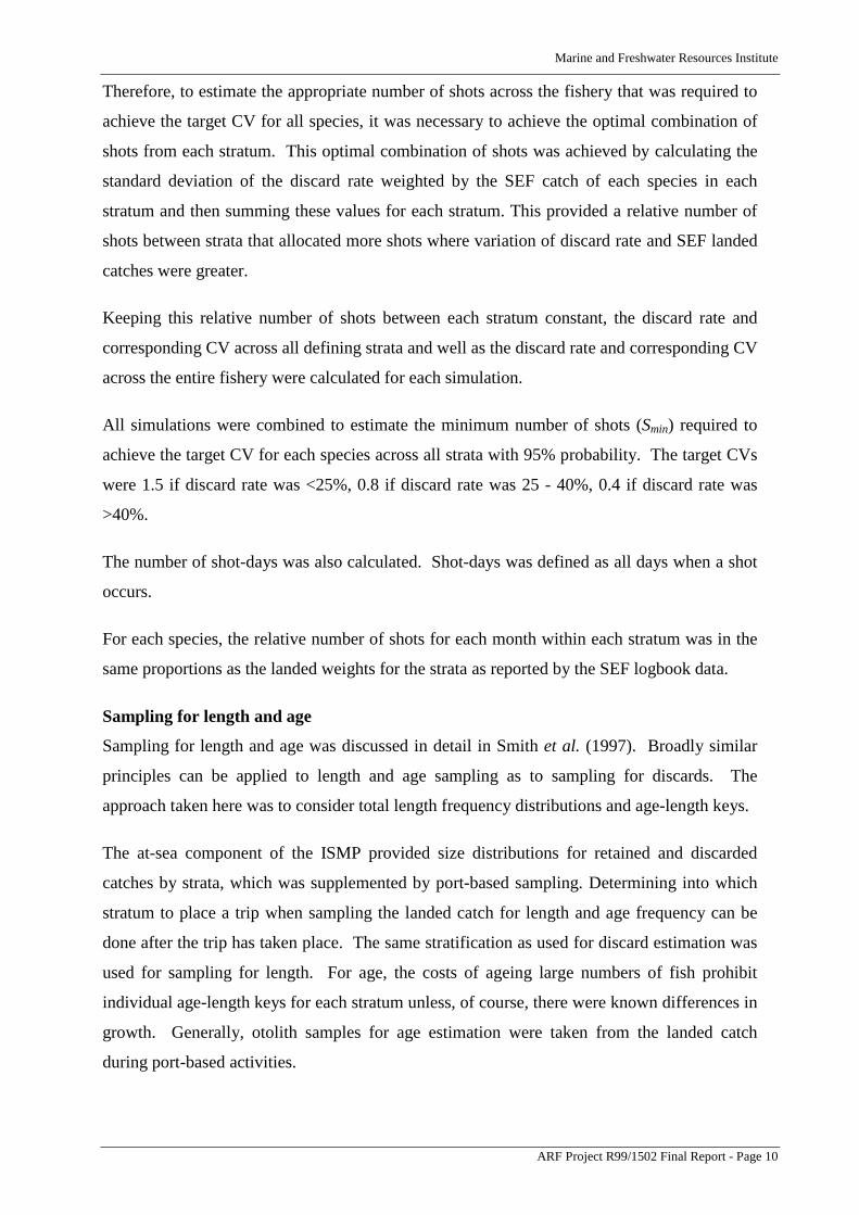
Therefore, to estimate the appropriate number of shots across the fishery that was required to
achieve the target CV for all species, it was necessary to achieve the optimal combination of
shots from each stratum. This optimal combination of shots was achieved by calculating the
standard deviation of the discard rate weighted by the SEF catch of each species in each
stratum and then summing these values for each stratum. This provided a relative number of
shots between strata that allocated more shots where variation of discard rate and SEF landed
catches were greater.
Keeping this relative number of shots between each stratum constant, the discard rate and
corresponding CV across all defining strata and well as the discard rate and corresponding CV
across the entire fishery were calculated for each simulation.
All simulations were combined to estimate the minimum number of shots (Smin) required to
achieve the target CV for each species across all strata with 95% probability. The target CVs
were 1.5 if discard rate was <25%, 0.8 if discard rate was 25 - 40%, 0.4 if discard rate was
>40%.
The number of shot-days was also calculated. Shot-days was defined as all days when a shot
occurs.
For each species, the relative number of shots for each month within each stratum was in the
same proportions as the landed weights for the strata as reported by the SEF logbook data.
Sampling for length and age
Sampling for length and age was discussed in detail in Smith et al. (1997). Broadly similar
principles can be applied to length and age sampling as to sampling for discards. The
approach taken here was to consider total length frequency distributions and age-length keys.
The at-sea component of the ISMP provided size distributions for retained and discarded
catches by strata, which was supplemented by port-based sampling. Determining into which
stratum to place a trip when sampling the landed catch for length and age frequency can be
done after the trip has taken place. The same stratification as used for discard estimation was
used for sampling for length. For age, the costs of ageing large numbers of fish prohibit
individual age-length keys for each stratum unless, of course, there were known differences in
growth. Generally, otolith samples for age estimation were taken from the landed catch
during port-based activities.

Marine and Freshwater Resources Institute
ARF Project R99/1502 Final Report - Page 11
Simulation modelling was used to assess the precision of sampling intensity for both lengths
and age-length keys. Methods were similar to those described by Sullivan et al. (1994). For
length frequency distributions, the data used for these simulations was taken from port-based
sampling and for the age-length keys, from the Central Ageing Facility database.
The estimated sample sizes for both age and particularly length, should be regarded as a
minimum.
Length frequency distributions.
The primary question when sampling catches to provide representative length frequency
distributions is how many samples are required and how many fish should be in each sample.
The simulation modelling was undertaken to provide a matrix of the number of samples
required and the corresponding number of fish in each sample.
For each simulation, a number of samples were randomly selected from all port samples (each
combination of callsign and date was considered one sample). The number of samples varied
in steps of 20, from 20 to 200. From these samples, a number of fish were randomly selected.
The number of fish per sample also varied in steps of 20, from 20 to 200. The mean weighted
coefficient of variation (MWCV) was calculated for each combination of sample size and
sample number.
A total of 500 simulations were completed for each combination and the MWCV calculated.
Optimal sample sizes for each number of samples were taken at the point at which the change
in MWCV was less than 1% for an increase of 20 in the number of fish in the sample. Larger
sample sizes give only a small increase in precision of the length frequency distribution.
Age-length keys
Smith et al. (1997) used similar simulations as described above to estimate the optimum
sample size for age-length keys for combined sexes and the sexes separately as appropriate.
However, in the case of age, only the total sample was considered. The range of sample sizes
was from 50 to 1500 in steps of 50. The optimal sample size was calculated as for length-
frequency samples but the sample size giving a MWCV of 10% was also calculated. This was
because in several cases the MWCV at the optimal sample size was greater than 10%.
Given the costs of ageing large numbers of fish, sampling by stratum was not considered.
Generally if there is no difference in a species’ growth between strata, age-length keys can be
applied broadly. However, the optimal sample size for both sexes combined should be
regarded as the absolute minimum. In addition, for species such as blue grenadier where

Marine and Freshwater Resources Institute
ARF Project R99/1502 Final Report - Page 12
growth is considerably different between sexes, the optimal sample size for each sex is the
more appropriate target.
RESULTS & DISCUSSIONData inputs
Merging SEF1 and SEF2 datasets
Due to errors and anomalies in the two datasets, data often could not be match-merged for a
given trip. Consequently, SEF1 and SEF2 data for each vessel were summed over the period
for which the vessel kept landing its catch at a given port to obtain a weighting factor for each
species caught by each vessel at a given port over that period. This weighting factor was then
applied to the SEF1 shot data to weight it up (or rarely down) to the SEF2 landings for each
species caught by each vessel in each port. This enabled merging of 99.5% of the SEF1 data
without the need to make subjective decisions in cases where SEF1 and SEF2 dates and
landings did not correspond. In the few cases (eg. 0.37% - 672 records out of 178 000 during
1999) in which quota species from a SEF1 shot could not be matched to a SEF2 landing,
those species catches for those shots were not included. This difference was then
compensated by the weighting factors from other shots.
Stratification
Smith et. al. (1997) used 14 strata to define the trawl fishery (Table 1). They noted, however,
that difficulties could result because the stratum into which a trip was placed was not finally
determined until landing, and the future sampling plan would need to be updated as a
consequence. We believe that the need for slight modifications to these strata have become
apparent over the last three years, mainly due to practical considerations of running the ISMP
and the changing dynamics of the fishery. The changes that we recommend and the
underlying reasons for changing the strata are outlined below.
The primary sampling unit
In the current ISMP sampling regime Smith et al. (1997) made the decision to use “trip”
rather than “shot” as the primary sampling unit because it was only practical for a sea-going
observer to sample whole trips. Indeed this is true, but changes in the fishery – especially the
tendency to target a larger variety of species for the markets – have resulted in a greater
variety of shots within a single trip. Over the last three years, there have been a number of
examples where stratification by trip rather than shot has resulted in “misclassification” of
shots into a particular stratum. For example, Knuckey and Sporcic (1999) highlighted a
Marine and Freshwater Resources Institute
ARF Project R99/1502 Final Report - Page 13
particular case where increasingly, inshore and offshore shots were being made in the same
trip off Eden/Lakes Entrance, but the trip then was classified as offshore. As a result, an
increasing proportion of the shots were effectively being misclassified, thereby creating noise
around the true estimates made for that stratum. Such noise reduced the effectiveness of the
stratification and the potential for simulation modelling to predict the correct sampling
intensity required to achieve target CVs for discard estimation. The use of shot as the primary
sampling unit eliminates misclassifications of shot into a stratum but, the trade-off is that the
observer has slightly less prior control over what strata may be sampled in any trip.
Therefore, although we recognised that the only way to sample a shot was by undertaking a
whole trip, we decided that shot was the more accurate and appropriate primary sampling unit
for the present study.
Fishing zone vs port
Smith et al. (1997) acknowledged that the zone fished would be a natural stratification
category but decided to reject it as impractical in favour of stratification by the port group in
which the fish were landed. They identified four port groups: NSW (Sydney to Bermagui);
EDEN/LAKES (Eden to Lakes Entrance); TAS (Tasmanian ports); and SW (Port Albert to
Adelaide) whose ports were geographically contiguous and harboured vessels which fish
similar species and areas. These groupings largely corresponded with the zones of fishing
and Smith et al. (1997) noted that in most instances, this would allow good estimates of
species by zone, if this was required. They further stated that practical difficulties with
stratification by zone included the sampler’s inability to determine where each vessel was
intending to fish before trips were selected, and the potential for a single fishing trip to span
two zones while the fish would only be landed and sampled on shore as a single group. Whilst
this is true, recent changes in the fishery have rendered these difficulties to be less of a
problem than using port as a stratification factor. The main reason for this was that in some
areas of the fishery, the previously strong relationship between port of landing and fishing
zone has tended to break down in recent years as fishers/owners make more dynamic decision
about where their vessels catch and land fish. Their decisions were based on a number of
factors including environmental conditions and their influence on catch rates, transport times
and costs, best market prices (Sydney vs Melbourne) and personal considerations such as
ensuring that crews regularly caught up with their families. Various examples of the
problems of using port as a proxy for fishing zone have been highlighted in the ISMP
progress reports and reports to SEFAG (eg. Knuckey and Sporcic 1999; Knuckey 2000). For
the above reasons, we have decided to redefine the spatial aspect of the strata to reflect the

Marine and Freshwater Resources Institute
ARF Project R99/1502 Final Report - Page 14
fishing region (NB. we have not used the term “zone” to minimise confusion with the zones
described by Klaer and Tilzey 1994) rather than port of landing and merge together the strata
where unique sub-fisheries have been split by port of landing.
Zones and nomenclature
Regions used to summarise the spatial distribution of sub-fisheries were first described by Klaer
and Tilzey (1994) and included Eastern Zone A, Eastern Zone B, Eastern Tasmania, Western
Tasmania, Western Zone and Bass Strait. The strata described by Smith et al. (1997) were more
detailed (including depth, port of landing and target fisheries), yet generally they still fitted well
within the previous divisions by zone. One slight discrepancy was that the NSW strata of
described by Smith et al. (1997) did not include Eden whereas the Eastern Zone A went down to
the NSW / Victoria border (37o 30’S), with Eastern Zone B being south of the border. The
decision to move away from port as a strata definition meant that we needed to apply some
division at the NSW / Victoria border. Analysis of effort data revealed that there was a natural
division in the fishery between Eden and Bermagui and that Smith’s NSW / EDL division better
reflected current fishing practices and known biology of fish resources in the area. As a
consequence it was decided that the dividing line for the new ISMP design should be between
Bermagui and Eden at (36o 45’S). To prevent confusion when drawing future comparisons, the
group decided that changing the names of statistical zones would be sensible. Reference to
Eastern Zone A and Eastern Zone B would now only relate to the historical analyses based on
Klaer and Tilzey’s 1994 fishery subregions, but would roughly correspond with the new NSW
and Eastern Victoria zones respectively. The changes adopted are shown below:
Current zone name New ISMP stratum name Geographical change
Bass Strait No change No change
Eastern zone A NSW South to 36o 45’S
Eastern zone B Eastern Victoria North to 36o 45’S
Western zone Western Victoria No change
Eastern Tasmania No change No change
Western Tasmania No change No change
Vessel capacity
Based on a suggestion by an external referee, Smith et al. (1997) used size of vessel landings
as a further stratification to increase sampling efficiency. SEF2 data were used to rank
Marine and Freshwater Resources Institute
ARF Project R99/1502 Final Report - Page 15
vessels in order of mean vessel landing per trip (all species, all fisheries). Vessels whose
mean landing fell below 5 tonnes per trip were denoted low vessels (lv) and the others were
denoted high vessels (hv). This division was used to subdivide two of the gear-fishery-port
strata (SW Other and EDEN/LAKES Inshore). It was not considered necessary for any of the
other strata. According to the observers, this has been the categorisation most difficult to
apply in a practical sense, but it has also been the most difficult to justify in a theoretical
sense. Part of the problem has been that, being based on an average, the hv/lv category did
not necessarily apply for any particular trip even though the boat was categorised as one or
the other. The other difficulty (especially in EDEN/LAKES) was that over the last few years,
boats have tended to leave their local fishing grounds during summer to take advantage of
better fishing conditions off the east coast of Tasmania. This has meant that they have been
making longer trips and catching more fish, which changes their hv/lv category. Thus, there
was a temporal influence which could change a vessel’s categorisation on both the short-term
(months) and long-term (years). This, we believe, made the hv/lv categorisation too
ephemeral to warrant its use in an ongoing stratification of the fishery and we have opted to
remove the hv/lv category.
Other trawl strata
Since July 2000, two extra trawl strata have been added to the ISMP in the SEF: East Coast
Deep Water (ECDW) and Victorian Inshore Trawl (VIT). Data on the level of monitoring
required in these strata was not available until September 2001. Nevertheless, as separate
sub-fisheries within the SEF, both strata will need to be included in any ongoing long-term
monitoring program for the SEF. At this stage we have simply opted to retain the sampling
intensity that has been agreed to by AFMA for 2000/01: 40 days for ECDW and 10 days for
VIT. Extra monitoring of the eastern gemfish spawning fishery was also undertaken by the
ISMP during 2000/01, but with only a bycatch TAC allowed for spawning gemfish and the
negligible catches of spawning fish taken during that year, this sub-fishery could not be
analysed as a separate stratum and will be incorporated into the NSW Offshore stratum.
Non-trawl
At sea monitoring of discard rates in the non-trawl fleet was not included in the ISMP
sampling regime designed by Smith et al. (1997) because data were limited for this sector and
discard rates were thought to be small. Since then, the Pilot Non-Trawl Monitoring Program
has been undertaken during 1999/2000 and information on the amount and composition of the
retained and discarded catches of SEF non-trawl vessels was now available (Knuckey et al.

Marine and Freshwater Resources Institute
ARF Project R99/1502 Final Report - Page 16
2001a). Compared to the trawl sector, non-trawl discard rates were generally low and precise
estimates did not require an extensive on-board monitoring program (Knuckey et al. 2001a).
Nevertheless, the South East Non-Trawl Management Advisory Committee (SENTMAC)
determined that a base level of independent on-board monitoring of the non-trawl fishery
should continue, at least to meet the requirements of strategic assessment.
The sampling plan used for the Pilot Monitoring Program was stratified by gear, region (port)
and season. Based on the results of that Program, similar stratification has been adopted for
the present study, except certain gear x region cells have been dropped because of negligible
fishing activities. Gear has been categorised into mesh net, dropline and longline and the
regional categories (similar to the trawl) of NSW, EDEN/LAKES, TAS and SOUTHWEST
have been retained (Table 4). Seasonal sampling intensity was divided amongst these strata
based simply on levels of fishing activity.
Stratification for the ISMP design model
The future stratification for on-board monitoring by the ISMP is presented in Table 4. It was
generally based on the initial stratification by Smith et al. (1997), but included the
modifications we have recommended after three years of ISMP operations, together with the
inclusion of other trawl and non-trawl strata.
All shots of SEF logbook and ISMP data were assigned a stratum. Strata were defined by the
fishing location, season, catch composition and/or gear. Any locations outside these
geographic locations were not included in the analysis. Each stratum for trawl and non-trawl
data were defined as presented in Table 4.
All of the proposed changes to the ISMP sampling regime highlighted above were presented
at the 2001 SEFAG Plenary. The reasons for the changes were discussed by the managers,
scientists and industry members present and were accepted.
Simulation modelling and estimation of discard rates and corresponding CVs
Simulations were performed on all years of the ISMP data but weighted so that shots from the
more recent years had a higher probability of being selected (Table 3). The results for all the
simulations were then used to investigate the distribution of the estimated discard rate CV for
each species for each number of shots within each stratum and then across the entire fishery.
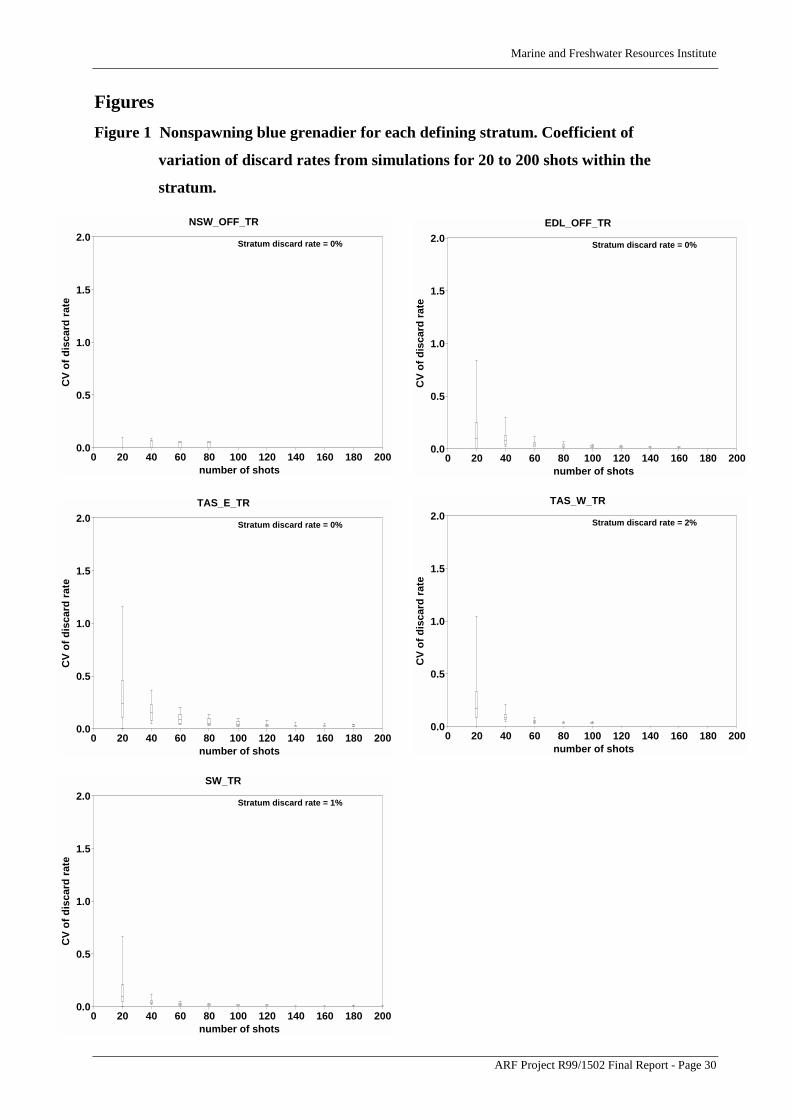
The results for each species in their defining strata (see Table 4) are presented in Figures 1 to
20. Each plot shows the minimum and maximum values of the discard rate CV as well as the
median and the interquartile range for different numbers of shots. The results for each species

Marine and Freshwater Resources Institute
ARF Project R99/1502 Final Report - Page 17
for the fishery (i.e. across all strata) are presented in Figures 21 to 40. The reference lines of
target CVs 1.5, 0.8 and 0.4 were included in the figures to indicate the number of shots
required to achieve the required target CV (as defined by discard rate – see Methods) with a
high probability. Note the number of shots on the graphs does not include the ‘Other’
stratum.
The minimum number of shots for each species within each stratum is presented in Table 5.
The proportion of successful shots (psucc) within each stratum is also presented. This is the
proportion of shots that contain each species. The actual number of shots required (Sreq) to
achieve the target CV for each species is therefore the number of shots necessary to achieve
the number of successful shots. These are presented in Table 6.
succreq p
SS min=
The number of shots required within a particular stratum was the maximum value of Sreq
across species within that stratum (Table 7). Based on the average number of shots completed
in a single day in each stratum, this converts to approximately 420 shot days (Table 7). Note
that this may not represent the total number of sea days because shots can be undertaken in
more than one stratum during any one day. Table 8 shows observed shots by month that
would be required in each stratum.
A particular difficulty in determining the shot allocation for any one strata was because it was
influenced by the variability within species across strata as well as the variation between
species within strata. One of the critical issues with the modelling was the way in which the
shots were allocated across the strata for each species. The initial problem encountered was
that the simulations would place all of the shots for a species within the stratum with the
highest discard variability. This was unacceptable, as it provided no way of including the
information available on the discard rates in other defining strata. The solution lay in
including a measure of the SEF catch in every defining stratum together with the discard rate.
There were a number of statistical ways that this could have been resolved. We chose to
calculate the standard deviation of the discard rate weighted by the SEF catch of each species
in each stratum and then sum these values for each stratum. Various other statistics were
explored to determine the relative allocation of shots. Most produced similar results as long
as the discard rate and SEF catch were included. Ultimately we chose the current statistic
because it was the most intuitive. Adoption of this method reduced computer processing time
considerably and enabled full automation of the procedure in a truly objective manner.
Marine and Freshwater Resources Institute
ARF Project R99/1502 Final Report - Page 18
Sampling for length and age
In general, the annual sample size required to obtain a representative length frequency sample
ranged between 2500 and 7000 fish. If each sample were to contain 100 – 150 fish, this would
require between 20 – 40 samples to be collected per year (Table 9). At this level of sampling
intensity CVs less than 0.1 can be easily achieved. What tends to happen in the stock assessment
process, however, is that scientists and managers require length frequency stratification beyond
that of the ISMP in order to account for divisions in stocks, regional boundaries or sexual
dimorphism etc. As a result, the sample numbers provided by the adaptive design project should
be considered as an absolute minimum and sampling within each stratum should endeavour to
cover full spatial and temporal ranges.
Ageing data is only required on a small number (ten) of all of the SEF quota species. The
sampling required for length frequency easily encompasses the number of samples needed to
provide representative age length keys for each of these species. These sample sizes
developed by Smith et al. (1997) were still applicable to the current design model, as age-
length keys have not changed for any of the species. In practice, the costs required to age the
samples is the main factor limiting the number of fish of each species that get aged. Each
year, SETMAC and AFMA, through consultation with the Central Ageing Facility determines
the species and the sample sizes to be aged. This is not a function of the ISMP and this
process could not readily be incorporated in a simulation model.
Implications of the design model for an adaptive ISMP sampling regime
In undertaking this project we have provided a means of efficiently updating the ISMP
sampling regime on a regular basis (most practically annual) to provide statistically robust
estimates of discard rates and length frequency distributions. By applying a relatively
automated process, it is now possible to alter the sampling regime to best suit the current
dynamics of the fishery. This will reduce most of the problems that were incurred previously
when the initial ISMP sampling became outdated with respect to the current fishery practices.
One of the advantages in having developed the SAS code to undertake such analyses of the
SEF data is that it can now be relatively easily altered to measure different fishery parameters
to determine the optimum sampling regime. Currently it uses discard rate CVs, but it could
easily be changed to optimise CVs for catch composition, CPUE, detection of listed species
etc. In this manner, the ISMP can maintain a sampling regime that meets the changing
requirement of management, scientists and industry. Furthermore, the required levels of
precision can be altered depending on the requirements or to the available budget.
Importantly for the current ISMP, the modified sampling regime determined in the current

Marine and Freshwater Resources Institute
ARF Project R99/1502 Final Report - Page 19
project is of a similar magnitude to that already operating. This means that it is possible to
adopt the adaptive sampling regime without large changes to the current budget or operating
procedures. It is important to note, however, that as a voluntary monitoring program the
current and proposed ISMP sampling methods rely entirely on comprehensive coverage of
most vessels operating in the SEF. To date this has been achieved to an extent where virtually
all CVs have been achieved. A similar level of acceptance and coverage will be required if
the adaptive sampling regime is to be successful.
Whilst there are a number of advantages in applying a relatively automated means of adapting
the ISMP sampling regime on an annual basis, it is worth pointing out some possible pitfalls.
The most obvious (and most concerning) would be the problems associated with “blindly”
accepting the results of the analyses without endeavouring to understand the underlying
dynamics of the fishery. The initial analysis undertaken for this project provides a good
example. The extremely high predicted sampling required in NSW_OFF_TR is a result of the
sampling requirements needed to estimate appropriate discard CVs for blue eye trevalla. It is
important to consider the underlying reasons that may be potentially driving this requirement.
Blue eye is one species for which there is often difficulty obtaining sufficient trawl quota.
This is likely to have a significant effect on discard levels and may cause high variability in
discard rates depending on the quota situation of the fisher. Also, blue eye trevalla are a
species that typically exhibits high levels of spatial and temporal structuring of the stocks, so
higher levels of length sampling are likely to be required to meet appropriate CV levels. How
important is the need to meet the CVs for this particular species in the NSW_OFF_TR
stratum – a stratum that only supplies a relatively small amount of the total blue eye catch?
Sampling in this stratum could be reduced considerably without the blue eye requirement.
Compromises are possible. A potential option would be to alter the CV required for this
species in this stratum or to remove blue eye as one of the defining species for this stratum
completely. It is important that such reasons and options for the ISMP adaptive sampling
regime are discussed prior to implementation. Ultimately, it will be the decision of a
combined industry/management/scientific group such as SEFAG on how to approach and
solve this type of issue.
One of the other issues associated with the implementation of the adaptive sampling regime is
the level of flexibility and uncertainty it brings into the process. With a set number of sea
days to achieve in each stratum, the current ISMP design is relatively easy to plan, cost and
carry out. If the number of shots required in any one stratum can potentially change from
year to year or changes across the entire fishery, it is far more difficult to plan the spatial and

Marine and Freshwater Resources Institute
ARF Project R99/1502 Final Report - Page 20
temporal requirements for human resources and to budget them accordingly. Costs associated
with getting ISMP scientists out on vessels increases markedly the further afield from their
own port they travel.
A table showing the achievement of the pro-rata (July to October 2001) target number of
shots (compared to days) for each stratum against those predicted by the model using 2000
data is provided (Table 10 - from Knuckey and Berrie 2001). This indicated that monitoring
of the NSW and Eastern Victoria offshore strata was tending to be greater than required,
whilst there was a shortfall of monitoring around western Tasmania. Although the ISMP
achieved all of the pro-rata target sea-days based on the initial design (against which the
current ISMP contract is measured), the discrepancy between the target and achieved number
of shots outlined using the design model highlighted the need for a dynamic approach to
monitoring of the SEF. It also shows that an adaptive sampling regime will require ISMP
staff to move around the fishery more than at present.
One important factor in the success of the current ISMP is the fact that field scientists
generally work from their home ports where they are familiar with the local fishers that they
go out with and have developed a level of trust over a period of years. As a voluntary
monitoring program, this issue can not be under-estimated – trust is important. One option to
allow for the flexibility in both staff numbers and location that may be required in an adaptive
management regime would be to opt for casual employees. It is difficult to determine what
impact this may have on the operational aspects of the ISMP and how well the industry
members would accept it. In a voluntary program, I tend to think that there may be benefits in
retaining known and trusted onboard scientists based in the fishing ports, even if the costs of
moving them around and maintaining them as full-time permanent staff is greater. It is a
difficult thing to test, but previous experience with the people required to undertake the tasks
required in the ISMP has shown that suitable people are few and far between.
Marine and Freshwater Resources Institute
ARF Project R99/1502 Final Report - Page 21
ReferencesKlaer, N.L. and Tilzey, R.D.J (1994). The multi-species structure of the fishery. In R.D.J.
Tilzey [ed.] The South East Fishery: A scientific review with particular reference to
quota management. Bureau of Resource Sciences Bulletin. Australian Government
Printer, Canberra.
Knuckey, I. A. (2000). South East Fishery Integrated Scientific Monitoring Program – 1999
Report to the South East Fishery Assessment Group. Australian Fisheries Management
Authority, Canberra. 91 pp.
Knuckey, I. A. and Berrie, S. E. (2001). South East Fishery Integrated Scientific Monitoring
Program – June to October 2001 Progress Report to the South East Fishery Assessment
Group. Australian Fisheries Management Authority, Canberra. 9 pp.
Knuckey, I. A., Berrie, S. E. and Gason, A. S. H. (2001). South East Fishery Integrated
Scientific Monitoring Program – 2000 Report to the South East Fishery Assessment
Group. Australian Fisheries Management Authority, Canberra. 107 pp.
Knuckey, I. A., Gill, S. and Gason, A. S. H. (2001a). South East Fishery Non-Trawl Pilot
Monitoring Program – Final Report to the Australian Fisheries Management Authority,
Canberra. 54 pp.
Knuckey, I. A. and Sporcic, M. I. (1999). South East Fishery Integrated Scientific Monitoring
Program – 1998 Report to the South East Fishery Assessment Group. Australian
Fisheries Management Authority, Canberra. 67 pp.
Smith, D.C., Gilbert D.J., Gason A. and Knuckey I. (1997) Design of an Integrated Scientific
Monitoring Programme for the South East Fishery - Final Report to the Australian
Fisheries Management Authority, Canberra.

Marine and Freshwater Resources Institute
ARF Project R99/1502 Final Report - Page 22
TablesTable 1 The initial definition of SEF strata used in the original ISMP design.
Stratification was based on gear type, main species caught, port group and size
of landings (after Smith et al. 1997).Stratum code Gear Port
group Defining species
OROSWall O. Trawl SW Orange roughy
OROTASall O. Trawl TAS Orange roughy
SBGSWall O. Trawl SW Blue grenadier (spawning)
SBGTASall O. Trawl TAS Blue grenadier (spawning)
OTHSWhv O. Trawl, highcatch vessels SW All species excl. roughy and spawning grenadier
OTHSWlv O. Trawl, lowcatch vessels SW All species excl. roughy and spawning grenadier
OTHTASall O. Trawl TAS All species excl. roughy and spawning grenadier
OFFSHEDLall O. Trawl EDENLAKES
Blue grenadier (non-spawning), gemfish, ling,ocean perch, mirror dory
OFFSHNSWall O. Trawl NSW Blue grenadier (non-spawning), gemfish, ling,ocean perch, mirror dory
INSHEDLhv O. Trawl, highcatch vessels
EDENLAKES
Spotted warehou, blue warehou, tiger flathead,jackass morwong, silver trevally, John dory andredfish
INSHEDLlv O. Trawl, lowcatch vessels
EDENLAKES
Spotted warehou, blue warehou, tiger flathead,jackass morwong, silver trevally, John dory andredfish
INSHNSWall O. Trawl NSWSpotted warehou, blue warehou, tiger flathead,jackass morwong, silver trevally, John dory andredfish
RRPall O. Trawl Royal red prawn
DSall D. Seine School whiting

Marine and Freshwater Resources Institute
ARF Project R99/1502 Final Report - Page 23
Table 2 Annual breakdown of trawl shots within each strata recorded by observers
from the ISMP.
Stratum name 1993 1994 1995 1996 1997 1998 1999 2000BS_IN_TR 0 0 14 1 0 0 3 9ECDW_TR 0 0 0 0 0 0 0 6EDL_DS 27 261 183 0 0 23 42 24EDL_IN_TR 0 52 42 44 150 94 98 75EDL_OFF_TR 0 37 25 27 53 98 66 53NSW_IN_TR 0 0 0 0 0 86 225 243NSW_OFF_TR 0 0 0 0 0 76 131 111NSW_RRP_TR 0 0 0 0 0 16 56 8OTHER 103 295 266 163 254 442 618 508SW_ORO_TR 0 36 0 0 11 10 2 4SW_TR 0 104 137 203 164 141 144 102TAS_BGS_TR 15 2 18 10 0 52 39 8TAS_E_TR 124 44 0 46 28 52 89 114TAS_ORO_TR 24 21 0 0 0 14 40 20TAS_W_TR 85 32 57 0 4 17 15 5
Table 3 The probability of selecting a shot from each year from the shots available.
YearProbability of selecting a shotfrom a specific year relative tothe most recent year
Distribution of shots from eachyear in the final sample
1993 0.26 10%1994 0.33 11%1995 0.41 13%1996 0.52 14%1997 0.64 16%
1998 (y-1) 0.80 17%1999 (y) 1.00 19%
Total 100%
Marine and Freshwater Resources Institute
ARF Project R99/1502 Final Report - Page 24
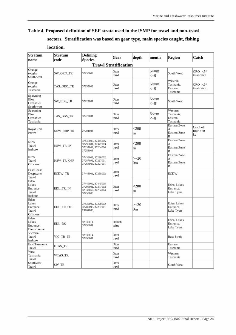
Table 4 Proposed definition of SEF strata used in the ISMP for trawl and non-trawl
sectors. Stratification was based on gear type, main species caught, fishing
location.Stratumname
Stratumcode
DefiningSpecies Gear depth month Region Catch
Trawl StratificationOrangeroughySouth west
SW_ORO_TR 37255009 Ottertrawl
6<=m<=9 South West ORO >.5*
total catch
OrangeroughyTasmania
TAS_ORO_TR 37255009 Ottertrawl
6<=m<=9
WesternTasmania,EasternTasmania
ORO >.5*total catch
SpawningBlueGrenadierSouth west
SW_BGS_TR 37227001 Ottertrawl
6<=m<=9 South West
SpawningBlueGrenadierTasmania
TAS_BGS_TR 37227001 Ottertrawl
6<=m<=8
WesternTasmania,EasternTasmania
Royal RedPrawn NSW_RRP_TR 27701004 Otter
trawl<200m
Eastern ZoneAEastern ZoneB
Catch ofRRP >50kg
NSWTrawlInshore
NSW_TR_IN37445006, 3744500537296001, 3737700337337062, 3726400437258003
Ottertrawl
<200m
Eastern ZoneAEastern ZoneB
NSWTrawlOffshore
NSW_TR_OFF37439002, 3722800237287093, 3728700137264003, 37227001
Ottertrawl
>=200m
Eastern ZoneAEastern ZoneB
East CoastDeepwaterTrawl
ECDW_TR 37445001, 37258002 Ottertrawl ECDW
EdenLakesEntranceTrawlInshore
EDL_TR_IN37445006, 3744500537296001, 3737700337337062, 3726400437258003
Ottertrawl
<200m
Eden, LakesEntrance,Lake Tyers
EdenLakesEntranceTrawlOffshore
EDL_TR_OFF37439002, 3722800237287093, 3728700123764003,
Ottertrawl
>=200m
Eden, LakesEntrance,Lake Tyers
EdenLakesEntranceDanish seine
EDL_DS 3733001437296001
Danishseine
Eden, LakesEntrance,Lake Tyers
VictoriaTrawlInshore
VIC_TR_IN 3733001437296001
Ottertrawl Bass Strait
East TasmaniaTrawl ETAS_TR Otter
trawlEasternTasmania
WestTasmaniaTrawl
WTAS_TR Ottertrawl
WesternTasmania
SouthwestTrawl SW_TR Otter
trawl South West
Marine and Freshwater Resources Institute
ARF Project R99/1502 Final Report - Page 25
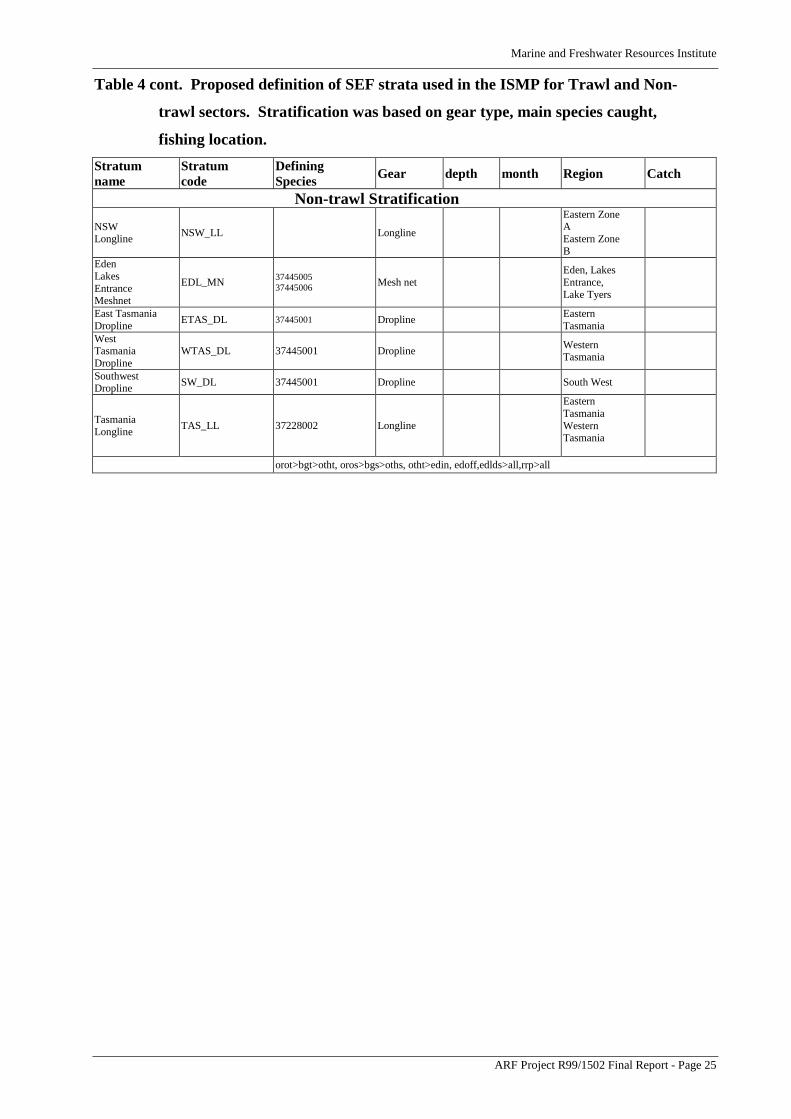
Table 4 cont. Proposed definition of SEF strata used in the ISMP for Trawl and Non-
trawl sectors. Stratification was based on gear type, main species caught,
fishing location.Stratumname
Stratumcode
DefiningSpecies Gear depth month Region Catch
Non-trawl StratificationNSWLongline NSW_LL Longline
Eastern ZoneAEastern ZoneB
EdenLakesEntranceMeshnet
EDL_MN 3744500537445006 Mesh net
Eden, LakesEntrance,Lake Tyers
East TasmaniaDropline ETAS_DL 37445001 Dropline Eastern
TasmaniaWestTasmaniaDropline
WTAS_DL 37445001 Dropline WesternTasmania
SouthwestDropline SW_DL 37445001 Dropline South West
TasmaniaLongline TAS_LL 37228002 Longline
EasternTasmaniaWesternTasmania
orot>bgt>otht, oros>bgs>oths, otht>edin, edoff,edlds>all,rrp>all

Marine and Freshwater Resources Institute
ARF Project R99/1502 Final Report - Page 26
Table 5 Minimum number of shots required (Smin) to achieve the target CV for eachspecies in their defining strata. Numbers in parentheses are the proportion ofshots that contain that species i.e. ‘successful’ shots (Psucc).
species NSW
INTR
EDL
IN
TR
NSW
OFF
TR
EDL
OFF
TR
NSW
RRP
TR
EDL
DS
TAS
E
TR
TAS
W
TR
SW
TR
TAS
ORO
TR
TAS
BGS
TR
TAS
BGS
TR
BS
IN
TR
ECDW
TR
OT
HE
R
Blue grenadier - nonspawning 0 0 1(.08) 14(.37) 0 0 11(.64) 13(.46) 19(.60) 0 0 0 0 0 1
Blue grenadier - spawning 0 0 0 0 0 0 0 0 0 0 0 26(1.0) 0 0 1
John dory 60(.93) 1(.93) 0 0 0 0 0 0 0 0 0 0 0 0 1
Mirror dory 0 0 7(.82) 8(.66) 0 0 7(.72) 5(.28) 3(.52) 0 0 0 0 0 4
Tiger flathead 3(.96) 10(1.0) 0 0 0 3(1.0) 1(.32) 1(1.0) 2(.16) 0 0 0 0 0 2
Eastern Gemfish 0 0 9(.65) 10(.53) 0 0 4(.30) 0 0 0 0 0 0 0 2
Western Gemfish 0 0 0 0 0 0 0 9(.13) 12(.57) 0 0 0 0 0 1
Pink Ling 0 0 6(.80) 13(.95) 0 0 20(.72) 8(.89) 12(.76) 0 0 0 0 0 10
Jackass morwong 4(.50) 14(.74) 0 0 0 0 8(.48) 1(.11) 4(.25) 0 0 0 0 0 5
Orange Roughy 0 0 0 0 0 0 0 0 0 31(1.0) 7(1.0) 0 0 0 9
Other 21(1.0) 21(1.0) 20(1.0) 20(1.0) 14(1.0) 20(1.0) 20(1.0) 19(1.0) 20(1.0) 14(1.0) 19(1.0) 21(1.0) 21(1.0) 22(1.0)
Redfish 13(.76) 1(.55) 0 0 0 0 0 0 0 0 0 0 0 0 1
Ocean perch - inshore 6(.58) 4(.86) 0 0 0 0 0 0 0 0 0 0 0 0 1
Ocean perch - offshore 0 0 5(.92) 6(.85) 0 0 7(.60) 6(.49) 6(.48) 0 0 0 0 0 1
Royal red prawn 0 0 0 0 9(1.0) 0 0 0 0 0 0 0 0 0 1
Blue eye Trevalla 0 0 25(.08) 4(.18) 0 0 10(.35) 8(.15) 12(.34) 0 0 0 0 0 25
Silver trevally 163(.48) 4(.26) 0 0 0 0 0 0 0 0 0 0 0 0 1
Spotted warehou 0 0 7(.20) 17(.59) 0 0 9(.70) 22(.34) 16(.71) 0 0 0 0 0 24
Blue Warehou 17(.10) 15(.41) 0 0 0 0 4(.22) 1(.07) 6(.29) 0 0 0 0 0 3
School whiting 0 0 0 0 0 12(.63) 0 0 0 0 0 0 0 0 1
Table 6 Actual number of shots required (Sreq) to achieve the target CV for each species
in their defining strata.spec NSW
INTR
EDLINTR
NSWOFFTR
EDLOFFTR
NSWRRPTR
EDLDS
TASE
TR
TASWTR
SWTR
TASOROTR
SWOROTR
TASBGSTR
BSINTR
ECDWTR
OTHER
Blue grenadier - nonspawning 0 0 7 36 0 0 17 28 30 0 0 0 0 0 1
Blue grenadier - spawning 0 0 0 0 0 0 0 0 0 0 0 26 0 0 1
John dory 64 1 0 0 0 0 0 0 0 0 0 0 0 0 1
Mirror dory 0 0 8 11 0 0 10 17 5 0 0 0 0 0 4
Tiger flathead 3 10 0 0 0 3 2 1 10 0 0 0 0 0 2
Eastern Gemfish 0 0 14 17 0 0 13 0 0 0 0 0 0 0 2
Western Gemfish 0 0 0 0 0 0 0 69 20 0 0 0 0 0 1
Pink Ling 0 0 7 14 0 0 27 9 16 0 0 0 0 0 10
Jackass morwong 7 18 0 0 0 0 16 1 14 0 0 0 0 0 5
Orange Roughy 0 0 0 0 0 0 0 0 0 31 7 0 0 0 9
Other 21 21 20 20 14 20 20 19 20 14 19 21 21 22
Redfish 16 1 0 0 0 0 0 0 0 0 0 0 0 0 1
Ocean perch - inshore 9 4 0 0 0 0 0 0 0 0 0 0 0 0 1
Ocean perch - offshore 0 0 5 7 0 0 10 12 11 0 0 0 0 0 1
Royal red prawn 0 0 0 0 9 0 0 0 0 0 0 0 0 0 1
Blue eye Trevalla 0 0 321 21 0 0 28 54 35 0 0 0 0 0 25
Silver trevally 340 15 0 0 0 0 0 0 0 0 0 0 0 0 1
Spotted warehou 0 0 34 29 0 0 13 62 23 0 0 0 0 0 24
Blue Warehou 155 35 0 0 0 0 18 9 19 0 0 0 0 0 3
School whiting 0 0 0 0 0 18 0 0 0 0 0 0 0 0 1
Marine and Freshwater Resources Institute
ARF Project R99/1502 Final Report - Page 27
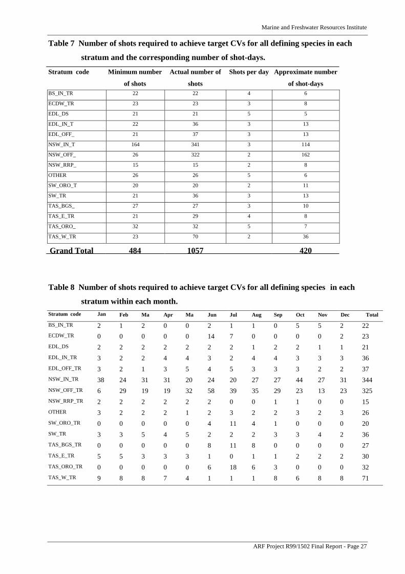
Table 7 Number of shots required to achieve target CVs for all defining species in each
stratum and the corresponding number of shot-days.
Stratum code Minimum number
of shots
Actual number of
shots
Shots per day Approximate number
of shot-daysBS_IN_TR 22 22 4 6
ECDW_TR 23 23 3 8
EDL_DS 21 21 5 5
EDL_IN_T 22 36 3 13
EDL_OFF_ 21 37 3 13
NSW_IN_T 164 341 3 114
NSW_OFF_ 26 322 2 162
NSW_RRP_ 15 15 2 8
OTHER 26 26 5 6
SW_ORO_T 20 20 2 11
SW_TR 21 36 3 13
TAS_BGS_ 27 27 3 10
TAS_E_TR 21 29 4 8
TAS_ORO_ 32 32 5 7
TAS_W_TR 23 70 2 36
Grand Total 484 1057 420
Table 8 Number of shots required to achieve target CVs for all defining species in each
stratum within each month.Stratum code Jan Feb Ma Apr Ma Jun Jul Aug Sep Oct Nov Dec Total
BS_IN_TR 2 1 2 0 0 2 1 1 0 5 5 2 22ECDW_TR 0 0 0 0 0 14 7 0 0 0 0 2 23EDL_DS 2 2 2 2 2 2 2 1 2 2 1 1 21EDL_IN_TR 3 2 2 4 4 3 2 4 4 3 3 3 36EDL_OFF_TR 3 2 1 3 5 4 5 3 3 3 2 2 37NSW_IN_TR 38 24 31 31 20 24 20 27 27 44 27 31 344NSW_OFF_TR 6 29 19 19 32 58 39 35 29 23 13 23 325NSW_RRP_TR 2 2 2 2 2 2 0 0 1 1 0 0 15OTHER 3 2 2 2 1 2 3 2 2 3 2 3 26SW_ORO_TR 0 0 0 0 0 4 11 4 1 0 0 0 20SW_TR 3 3 5 4 5 2 2 2 3 3 4 2 36TAS_BGS_TR 0 0 0 0 0 8 11 8 0 0 0 0 27TAS_E_TR 5 5 3 3 3 1 0 1 1 2 2 2 30TAS_ORO_TR 0 0 0 0 0 6 18 6 3 0 0 0 32TAS_W_TR 9 8 8 7 4 1 1 1 8 6 8 8 71

Marine and Freshwater Resources Institute
ARF Project R99/1502 Final Report - Page 28
Table 9 The mean weighted CV (in parentheses) of length frequencies for each
combination of number of fish and number of samples. Bold figures represent
the number of fish required for a minimum number of samples to achieve a
CV of 0.1.Number of samples
Species _20 40 _60 _80 _100 _140 _200
Blue Warehou 125(.07) 100(.04) 75(.03) 75(.02) 50(.02) 50(.02) 50(.01)
Blue eye Trevalla 125(.10) 125(.05) 75(.04) 75(.03) 75(.02) 50(.02) 50(.01)
Blue grenadier - nonspawning 125(.08) 100(.04) 75(.03) 75(.03) 75(.02) 50(.02) 50(.01)
Blue grenadier - spawning 175(.12) 150(.06) 100(.05) 75(.04) 75(.04) 75(.03) 50(.02)
Eastern Gemfish 200(.14) 150(.08) 100(.06) 100(.05) 100(.04) 75(.03) 75(.02)
Jackass morwong 125(.08) 100(.04) 75(.03) 75(.02) 75(.02) 50(.02) 50(.01)
John dory 150(.12) 125(.06) 100(.04) 100(.03) 75(.03) 75(.02) 50(.02)
Mirror dory 175(.16) 125(.10) 100(.07) 100(.05) 75(.05) 75(.03) 75(.02)
Ocean perch - inshore 0 175(.10) 125(.08) 100(.07) 100(.05) 75(.04) 75(.03)
Ocean perch - offshore 200(.13) 125(.08) 125(.05) 100(.04) 75(.04) 75(.03) 75(.02)
Orange Roughy 150(.07) 100(.05) 75(.03) 75(.03) 50(.03) 50(.02) 50(.01)
Pink Ling 150(.13) 100(.07) 100(.05) 75(.04) 75(.03) 75(.02) 50(.02)
Redfish 175(.12) 125(.07) 100(.05) 75(.04) 75(.03) 75(.02) 50(.02)
Royal red prawn 0 200(.14) 125(.12) 125(.09) 100(.08) 100(.06) 75(.04)
School whiting 175(.08) 100(.06) 75(.04) 75(.03) 75(.03) 50(.02) 50(.02)
Silver trevally 0 150(.10) 125(.08) 100(.06) 100(.05) 100(.04) 75(.03)
Spotted warehou 125(.07) 100(.04) 75(.03) 50(.03) 50(.02) 50(.01) 50(.01)
Tiger flathead 125(.07) 75(.04) 75(.03) 75(.02) 50(.02) 50(.01) 50(.01)
Western Gemfish 150(.09) 100(.05) 75(.04) 75(.03) 75(.02) 50(.02) 50(.01)

Marine and Freshwater Resources Institute
ARF Project R99/1502 Final Report - Page 29
Table 10 Summary of the number of shots undertaken by on-board observers during
July to October 2001 against pro-rata target shots as estimated using the ISMP
design model for 2000 data.
Region Strata Annual
Target
No. of shots
Pro-rata
Target
No. of shots
Number of
shots
monitored
Difference
NSW Inshore 239 89 86 -3Offshore 23* (615) 8*(262) 57 +49*(-205)
Royal RedPrawn
18 3 3 0
ECDW# 40 days 13 0 -13 daysVIC East Inshore 210 79 75 -4
Offshore 42 17 53 +36DanishSeine
45 14 14 0
Bass Strait VIT# 20 days 7 1 day -6 daysTAS East 52 6 0 -6
West 108 35 18 -17Orangeroughy
20 17 22 +5
Spawninggrenadier
46 33 42 +9
VIC West Other 66 21 29 +8Orangeroughy
6 5 8 +3
TOTAL 875 314 366 +52
*Number of shots required if reduced sampling for blue eye trevalla in NSW_OFF_TR be accepted. Number in
parentheses indicates shots required by ISMP design model if full blue eye coverage is estimated.
#The ECDW and VIT strata were not included in the ISMP design model estimations.
Marine and Freshwater Resources Institute
ARF Project R99/1502 Final Report - Page 30
FiguresFigure 1 Nonspawning blue grenadier for each defining stratum. Coefficient of
variation of discard rates from simulations for 20 to 200 shots within the
stratum.
Stratum discard rate = 0%
NSW_OFF_TR
CV
of d
isca
rd ra
te
0.0
0.5
1.0
1.5
2.0
number of shots0 20 40 60 80 100 120 140 160 180 200
Stratum discard rate = 0%
EDL_OFF_TR
CV
of d
isca
rd ra
te
0.0
0.5
1.0
1.5
2.0
number of shots0 20 40 60 80 100 120 140 160 180 200
Stratum discard rate = 1%
SW_TR
CV
of d
isca
rd ra
te
0.0
0.5
1.0
1.5
2.0
number of shots0 20 40 60 80 100 120 140 160 180 200
Stratum discard rate = 0%
TAS_E_TR
CV
of d
isca
rd ra
te
0.0
0.5
1.0
1.5
2.0
number of shots0 20 40 60 80 100 120 140 160 180 200
Stratum discard rate = 2%
TAS_W_TR
CV
of d
isca
rd ra
te
0.0
0.5
1.0
1.5
2.0
number of shots0 20 40 60 80 100 120 140 160 180 200

Marine and Freshwater Resources Institute
ARF Project R99/1502 Final Report - Page 31
Figure 2 Spawning blue grenadier for each defining stratum. Coefficient of variation of
discard rates from simulations for 20 to 200 shots within the stratum.
Stratum discard rate = 15%
spec=bgs SW_TR
CV
of d
isca
rd ra
te
0.0
0.5
1.0
1.5
2.0
2.5
3.0
number of shots0 20 40 60 80 100 120 140 160 180 200
Stratum discard rate = 2%
spec=bgs TAS_BGS_TR
CV
of d
isca
rd ra
te
0.0
0.5
1.0
1.5
2.0
2.5
3.0
number of shots0 20 40 60 80 100 120 140 160 180 200

Marine and Freshwater Resources Institute
ARF Project R99/1502 Final Report - Page 32
Figure 3 John dory for each defining stratum. Coefficient of variation of discard rates
from simulations for 20 to 200 shots within the stratum.
Stratum discard rate = 7%
spec=doj EDL_IN_TR
CV
of d
isca
rd ra
te
0
5
10
15
number of shots0 20 40 60 80 100 120 140 160 180 200
Stratum discard rate = 0%
spec=doj NSW_IN_TR
CV
of d
isca
rd ra
te
0
5
10
15
number of shots0 20 40 60 80 100 120 140 160 180 200
Stratum discard rate = 0%
spec=doj SW_TR
CV
of d
isca
rd ra
te0
5
10
15
number of shots0 20 40 60 80 100 120 140 160 180 200
Stratum discard rate = .%
spec=doj TAS_W_TR
CV
of d
isca
rd ra
te
0
5
10
15
number of shots0 20 40 60 80 100 120 140 160 180 200
Stratum discard rate = 0%
spec=doj TAS_E_TR
CV
of d
isca
rd ra
te
0
5
10
15
number of shots0 20 40 60 80 100 120 140 160 180 200

Marine and Freshwater Resources Institute
ARF Project R99/1502 Final Report - Page 33
Figure 4 Mirror dory for each defining stratum. Coefficient of variation of discard rates
from simulations for 20 to 200 shots within the stratum.
Stratum discard rate = 58%
spec=dom EDL_OFF_TR
CV
of d
isca
rd ra
te
0.0
0.5
1.0
1.5
number of shots0 20 40 60 80 100 120 140 160 180 200
Stratum discard rate = 27%
spec=dom NSW_OFF_TR
CV
of d
isca
rd ra
te
0.0
0.5
1.0
1.5
number of shots0 20 40 60 80 100 120 140 160 180 200
Stratum discard rate = 4%
spec=dom SW_TR
CV
of d
isca
rd ra
te0.0
0.5
1.0
1.5
number of shots0 20 40 60 80 100 120 140 160 180 200
Stratum discard rate = 66%
spec=dom TAS_E_TR
CV
of d
isca
rd ra
te
0.0
0.5
1.0
1.5
number of shots0 20 40 60 80 100 120 140 160 180 200
Stratum discard rate = 3%
spec=dom TAS_W_TR
CV
of d
isca
rd ra
te
0.0
0.5
1.0
1.5
number of shots0 20 40 60 80 100 120 140 160 180 200

Marine and Freshwater Resources Institute
ARF Project R99/1502 Final Report - Page 34
Figure 5 Flathead for each defining stratum. Coefficient of variation of discard rates
from simulations for 20 to 200 shots within the stratum.
Stratum discard rate = 5%
spec=flt EDL_DS
CV
of d
isca
rd ra
te
0.0
0.5
1.0
1.5
number of shots0 20 40 60 80 100 120 140 160 180 200
Stratum discard rate = 8%
spec=flt EDL_IN_TR
CV
of d
isca
rd ra
te
0.0
0.5
1.0
1.5
number of shots0 20 40 60 80 100 120 140 160 180 200
Stratum discard rate = 0%
spec=flt SW_TR
CV
of d
isca
rd ra
te
0.0
0.5
1.0
1.5
number of shots0 20 40 60 80 100 120 140 160 180 200
Stratum discard rate = 19%
spec=flt NSW_IN_TR
CV
of d
isca
rd ra
te
0.0
0.5
1.0
1.5
number of shots0 20 40 60 80 100 120 140 160 180 200
Stratum discard rate = 0%
spec=flt TAS_W_TR
CV
of d
isca
rd ra
te
0.0
0.5
1.0
1.5
number of shots0 20 40 60 80 100 120 140 160 180 200
Stratum discard rate = 0%
spec=flt TAS_E_TR
CV
of d
isca
rd ra
te
0.0
0.5
1.0
1.5
number of shots0 20 40 60 80 100 120 140 160 180 200

Marine and Freshwater Resources Institute
ARF Project R99/1502 Final Report - Page 35
Figure 6 Western gemfish for each defining stratum. Coefficient of variation of discard
rates from from simulations for 20 to 200 shots within the stratum.
Stratum discard rate = 5%
spec=gew SW_TR
CV
of d
isca
rd ra
te
0.0
0.5
1.0
1.5
number of shots0 20 40 60 80 100 120 140 160 180 200
Stratum discard rate = 0%
spec=gew TAS_W_TR
CV
of d
isca
rd ra
te0.0
0.5
1.0
1.5
number of shots0 20 40 60 80 100 120 140 160 180 200

Marine and Freshwater Resources Institute
ARF Project R99/1502 Final Report - Page 36
Figure 7 Eastern gemfish for each defining stratum. Coefficient of variation of discard
rates from simulations for 20 to 200 shots within the stratum.
Stratum discard rate = 14%
spec=gee EDL_OFF_TR
CV
of d
isca
rd ra
te
0.0
0.5
1.0
1.5
number of shots0 20 40 60 80 100 120 140 160 180 200
Stratum discard rate = 9%
spec=gee NSW_OFF_TR
CV
of d
isca
rd ra
te
0.0
0.5
1.0
1.5
number of shots0 20 40 60 80 100 120 140 160 180 200
Stratum discard rate = 11%
spec=gee TAS_E_TR
CV
of d
isca
rd ra
te0.0
0.5
1.0
1.5
number of shots0 20 40 60 80 100 120 140 160 180 200

Marine and Freshwater Resources Institute
ARF Project R99/1502 Final Report - Page 37
Figure 8 Ling for each defining stratum. Coefficient of variation of discard rates from
simulations for 20 to 200 shots within the stratum.
Stratum discard rate = 2%
spec=lig EDL_OFF_TR
CV
of d
isca
rd ra
te
0.0
0.5
1.0
1.5
number of shots0 20 40 60 80 100 120 140 160 180 200
Stratum discard rate = 4%
spec=lig TAS_E_TR
CV
of d
isca
rd ra
te
0.0
0.5
1.0
1.5
number of shots0 20 40 60 80 100 120 140 160 180 200
Stratum discard rate = 0%
spec=lig NSW_OFF_TR
CV
of d
isca
rd ra
te
0.0
0.5
1.0
1.5
number of shots0 20 40 60 80 100 120 140 160 180 200
Stratum discard rate = 1%
spec=lig SW_TR
CV
of d
isca
rd ra
te0.0
0.5
1.0
1.5
number of shots0 20 40 60 80 100 120 140 160 180 200
Stratum discard rate = 1%
spec=lig TAS_W_TR
CV
of d
isca
rd ra
te
0.0
0.5
1.0
1.5
number of shots0 20 40 60 80 100 120 140 160 180 200

Marine and Freshwater Resources Institute
ARF Project R99/1502 Final Report - Page 38
Figure 9 Jackass morwong for each defining stratum. Coefficient of variation of discard
rates from simulations for 20 to 200 shots within the stratum.
Stratum discard rate = 6%
spec=mow EDL_IN_TR
CV
of d
isca
rd ra
te
0.0
0.5
1.0
1.5
number of shots0 20 40 60 80 100 120 140 160 180 200
Stratum discard rate = 1%
spec=mow NSW_IN_TR
CV
of d
isca
rd ra
te
0.0
0.5
1.0
1.5
number of shots0 20 40 60 80 100 120 140 160 180 200
Stratum discard rate = 1%
spec=mow SW_TR
CV
of d
isca
rd ra
te
0.0
0.5
1.0
1.5
number of shots0 20 40 60 80 100 120 140 160 180 200
Stratum discard rate = 6%
spec=mow TAS_E_TR
CV
of d
isca
rd ra
te
0.0
0.5
1.0
1.5
number of shots0 20 40 60 80 100 120 140 160 180 200
Stratum discard rate = 0%
spec=mow TAS_W_TR
CV
of d
isca
rd ra
te
0.0
0.5
1.0
1.5
number of shots0 20 40 60 80 100 120 140 160 180 200
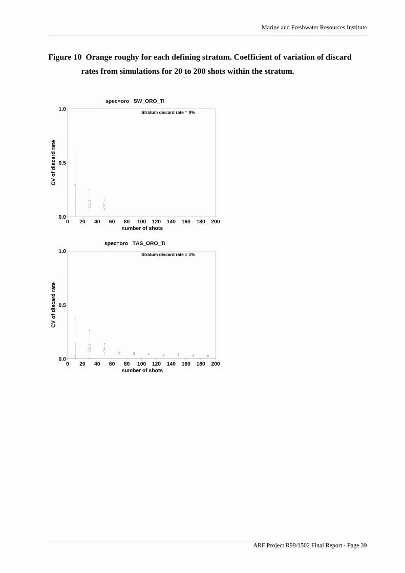
Marine and Freshwater Resources Institute
ARF Project R99/1502 Final Report - Page 39
Figure 10 Orange roughy for each defining stratum. Coefficient of variation of discard
rates from simulations for 20 to 200 shots within the stratum.
Stratum discard rate = 0%
spec=oro SW_ORO_TR
CV
of d
isca
rd ra
te
0.0
0.5
1.0
number of shots0 20 40 60 80 100 120 140 160 180 200
Stratum discard rate = 1%
spec=oro TAS_ORO_TR
CV
of d
isca
rd ra
te
0.0
0.5
1.0
number of shots0 20 40 60 80 100 120 140 160 180 200

Marine and Freshwater Resources Institute
ARF Project R99/1502 Final Report - Page 40
Figure 11 Other species for each stratum. Coefficient of variation of discard rates from
simulations for 20 to 200 shots within the stratum.
Stratum discard rate = 63%
spec=oth BS_IN_TR
CV
of d
isca
rd ra
te
0
2
4
6
number of shots0 20 40 60 80 100 120 140 160 180 200
Stratum discard rate = 61%
spec=oth NSW_IN_TR
CV
of d
isca
rd ra
te
0
2
4
6
number of shots0 20 40 60 80 100 120 140 160 180 200
Stratum discard rate = 66%
spec=oth SW_TR
CV
of d
isca
rd ra
te
0
2
4
6
number of shots0 20 40 60 80 100 120 140 160 180 200
Stratum discard rate = 84%
spec=oth TAS_ORO_TR
CV
of d
isca
rd ra
te
0
2
4
6
number of shots0 20 40 60 80 100 120 140 160 180 200
Stratum discard rate = 78%
spec=oth EDL_IN_TR
CV
of d
isca
rd ra
te
0
2
4
6
number of shots0 20 40 60 80 100 120 140 160 180 200
Stratum discard rate = 67%
spec=oth TAS_E_TR
CV
of d
isca
rd ra
te
0
2
4
6
number of shots0 20 40 60 80 100 120 140 160 180 200

Marine and Freshwater Resources Institute
ARF Project R99/1502 Final Report - Page 41
Stratum discard rate = 80%
spec=oth EDL_DS
CV
of d
isca
rd ra
te
0
2
4
6
number of shots0 20 40 60 80 100 120 140 160 180 200
Stratum discard rate = 63%
spec=oth EDL_OFF_TR
CV
of d
isca
rd ra
te
0
2
4
6
number of shots0 20 40 60 80 100 120 140 160 180 200
Stratum discard rate = 85%
spec=oth NSW_RRP_TRC
V of
dis
card
rate
0
2
4
6
number of shots0 20 40 60 80 100 120 140 160 180 200
Stratum discard rate = 61%
spec=oth TAS_BGS_TR
CV
of d
isca
rd ra
te
0
2
4
6
number of shots0 20 40 60 80 100 120 140 160 180 200
Stratum discard rate = 55%
spec=oth TAS_W_TR
CV
of d
isca
rd ra
te
0
2
4
6
number of shots0 20 40 60 80 100 120 140 160 180 200
Stratum discard rate = 52%
spec=oth SW_ORO_TR
CV
of d
isca
rd ra
te
0
2
4
6
number of shots0 20 40 60 80 100 120 140 160 180 200

Marine and Freshwater Resources Institute
ARF Project R99/1502 Final Report - Page 42
Stratum discard rate = 7%
spec=oth ECDW_TR
CV
of d
isca
rd ra
te
0
2
4
6
number of shots0 20 40 60 80 100 120 140 160 180 200
Stratum discard rate = 63%
spec=oth NSW_OFF_TR
CV
of d
isca
rd ra
te
0
2
4
6
number of shots0 20 40 60 80 100 120 140 160 180 200

Marine and Freshwater Resources Institute
ARF Project R99/1502 Final Report - Page 43
Figure 12 Redfish for each defining stratum. Coefficient of variation of discard rates
from simulations for 20 to 200 shots within the stratum.
Stratum discard rate = 0%
spec=red TAS_E_TR
CV
of d
isca
rd ra
te
0.0
0.5
1.0
1.5
2.0
number of shots0 20 40 60 80 100 120 140 160 180 200
Stratum discard rate = 51%
spec=red EDL_IN_TR
CV
of d
isca
rd ra
te
0.0
0.5
1.0
1.5
2.0
number of shots0 20 40 60 80 100 120 140 160 180 200
Stratum discard rate = 44%
spec=red NSW_IN_TR
CV
of d
isca
rd ra
te
0.0
0.5
1.0
1.5
2.0
number of shots0 20 40 60 80 100 120 140 160 180 200

Marine and Freshwater Resources Institute
ARF Project R99/1502 Final Report - Page 44
Figure 13 Inshore ocean perch for each defining stratum. Coefficient of variation of
discard rates from simulations for 20 to 200 shots within the stratum.
Stratum discard rate = 80%
spec=rei EDL_IN_TR
CV
of d
isca
rd ra
te
0.00
0.25
0.50
number of shots0 20 40 60 80 100 120 140 160 180 200
Stratum discard rate = 85%
spec=rei TAS_E_TR
CV
of d
isca
rd ra
te0.00
0.25
0.50
number of shots0 20 40 60 80 100 120 140 160 180 200
Stratum discard rate = 53%
spec=rei NSW_IN_TR
CV
of d
isca
rd ra
te
0.00
0.25
0.50
number of shots0 20 40 60 80 100 120 140 160 180 200
Stratum discard rate = 69%
spec=rei SW_TR
CV
of d
isca
rd ra
te
0.00
0.25
0.50
number of shots0 20 40 60 80 100 120 140 160 180 200

Marine and Freshwater Resources Institute
ARF Project R99/1502 Final Report - Page 45
Figure 14 Offshore ocean perch for each defining stratum. Coefficient of variation of
discard rates from simulations for 20 to 200 shots within the stratum.
Stratum discard rate = 21%
spec=reo EDL_OFF_TR
CV
of d
isca
rd ra
te
0.0
0.5
1.0
1.5
number of shots0 20 40 60 80 100 120 140 160 180 200
Stratum discard rate = 6%
spec=reo NSW_OFF_TR
CV
of d
isca
rd ra
te
0.0
0.5
1.0
1.5
number of shots0 20 40 60 80 100 120 140 160 180 200
Stratum discard rate = 19%
spec=reo SW_TR
CV
of d
isca
rd ra
te
0.0
0.5
1.0
1.5
number of shots0 20 40 60 80 100 120 140 160 180 200
Stratum discard rate = 26%
spec=reo TAS_E_TRC
V of
dis
card
rate
0.0
0.5
1.0
1.5
number of shots0 20 40 60 80 100 120 140 160 180 200
Stratum discard rate = 25%
spec=reo TAS_W_TR
CV
of d
isca
rd ra
te
0.0
0.5
1.0
1.5
number of shots0 20 40 60 80 100 120 140 160 180 200

Marine and Freshwater Resources Institute
ARF Project R99/1502 Final Report - Page 46
Figure 15 Royal red prawn for each defining stratum. Coefficient of variation of
discard rates from simulations for 20 to 200 shots within the stratum.
Stratum discard rate = 8%
spec=rrp NSW_RRP_TR
CV
of d
isca
rd ra
te
0.0
0.5
1.0
number of shots0 20 40 60 80 100 120 140 160 180 200
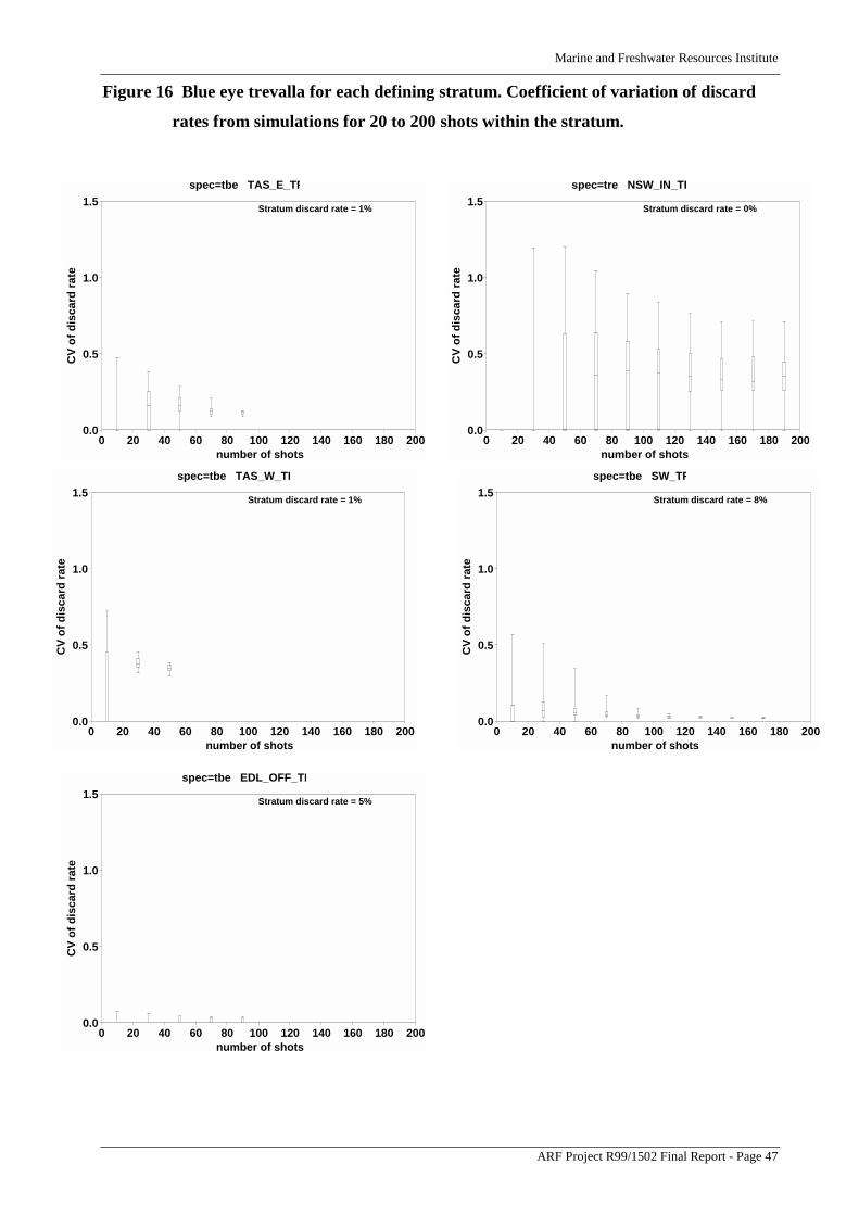
Marine and Freshwater Resources Institute
ARF Project R99/1502 Final Report - Page 47
Figure 16 Blue eye trevalla for each defining stratum. Coefficient of variation of discard
rates from simulations for 20 to 200 shots within the stratum.
Stratum discard rate = 1%
spec=tbe TAS_E_TR
CV
of d
isca
rd ra
te
0.0
0.5
1.0
1.5
number of shots0 20 40 60 80 100 120 140 160 180 200
Stratum discard rate = 5%
spec=tbe EDL_OFF_TR
CV
of d
isca
rd ra
te
0.0
0.5
1.0
1.5
number of shots0 20 40 60 80 100 120 140 160 180 200
Stratum discard rate = 1%
spec=tbe TAS_W_TR
CV
of d
isca
rd ra
te
0.0
0.5
1.0
1.5
number of shots0 20 40 60 80 100 120 140 160 180 200
Stratum discard rate = 0%
spec=tre NSW_IN_TR
CV
of d
isca
rd ra
te
0.0
0.5
1.0
1.5
number of shots0 20 40 60 80 100 120 140 160 180 200
Stratum discard rate = 8%
spec=tbe SW_TRC
V of
dis
card
rate
0.0
0.5
1.0
1.5
number of shots0 20 40 60 80 100 120 140 160 180 200

Marine and Freshwater Resources Institute
ARF Project R99/1502 Final Report - Page 48
Figure 17 Silver Trevally for each defining stratum. Coefficient of variation of discard
rates from simulations for 20 to 200 shots within the stratum.
Stratum discard rate = 2%
spec=tre EDL_IN_TR
CV
of d
isca
rd ra
te
0.0
0.5
1.0
1.5
number of shots0 20 40 60 80 100 120 140 160 180 200
Stratum discard rate = 0%
spec=tre NSW_IN_TR
CV
of d
isca
rd ra
te
0.0
0.5
1.0
1.5
number of shots0 20 40 60 80 100 120 140 160 180 200
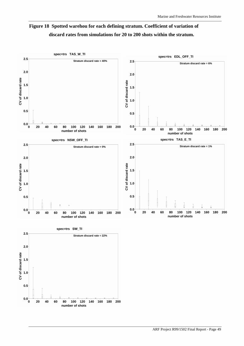
Marine and Freshwater Resources Institute
ARF Project R99/1502 Final Report - Page 49
Figure 18 Spotted warehou for each defining stratum. Coefficient of variation of
discard rates from simulations for 20 to 200 shots within the stratum.
Stratum discard rate = 6%
spec=trs EDL_OFF_TR
CV
of d
isca
rd ra
te0.0
0.5
1.0
1.5
2.0
2.5
number of shots0 20 40 60 80 100 120 140 160 180 200
Stratum discard rate = 0%
spec=trs NSW_OFF_TR
CV
of d
isca
rd ra
te
0.0
0.5
1.0
1.5
2.0
2.5
number of shots0 20 40 60 80 100 120 140 160 180 200
Stratum discard rate = 22%
spec=trs SW_TR
CV
of d
isca
rd ra
te
0.0
0.5
1.0
1.5
2.0
2.5
number of shots0 20 40 60 80 100 120 140 160 180 200
Stratum discard rate = 40%
spec=trs TAS_W_TR
CV
of d
isca
rd ra
te
0.0
0.5
1.0
1.5
2.0
2.5
number of shots0 20 40 60 80 100 120 140 160 180 200
Stratum discard rate = 1%
spec=trs TAS_E_TR
CV
of d
isca
rd ra
te
0.0
0.5
1.0
1.5
2.0
2.5
number of shots0 20 40 60 80 100 120 140 160 180 200

Marine and Freshwater Resources Institute
ARF Project R99/1502 Final Report - Page 50
Figure 19 Blue warehou for each defining stratum. Coefficient of variation of discard
rates from simulations for 20 to 200 shots within the stratum.
Stratum discard rate = 5%
spec=trt EDL_IN_TR
CV
of d
isca
rd ra
te
0.0
0.5
1.0
1.5
2.0
2.5
3.0
number of shots0 20 40 60 80 100 120 140 160 180 200
Stratum discard rate = 7%
spec=trt NSW_IN_TR
CV
of d
isca
rd ra
te
0.0
0.5
1.0
1.5
2.0
2.5
3.0
number of shots0 20 40 60 80 100 120 140 160 180 200
Stratum discard rate = 19%
spec=trt SW_TR
CV
of d
isca
rd ra
te
0.0
0.5
1.0
1.5
2.0
2.5
3.0
number of shots0 20 40 60 80 100 120 140 160 180 200
Stratum discard rate = 6%
spec=trt TAS_E_TR
CV
of d
isca
rd ra
te0.0
0.5
1.0
1.5
2.0
2.5
3.0
number of shots0 20 40 60 80 100 120 140 160 180 200
Stratum discard rate = 0%
spec=trt TAS_W_TR
CV
of d
isca
rd ra
te
0.0
0.5
1.0
1.5
2.0
2.5
3.0
number of shots0 20 40 60 80 100 120 140 160 180 200

Marine and Freshwater Resources Institute
ARF Project R99/1502 Final Report - Page 51
Figure 20 School whiting for each defining stratum. Coefficient of variation of discard
rates from simulations for 20 to 200 shots within the stratum.
Stratum discard rate = 2%
spec=whs EDL_DS
CV
of d
isca
rd ra
te
0.0
0.5
1.0
1.5
number of shots0 20 40 60 80 100 120 140 160 180 200
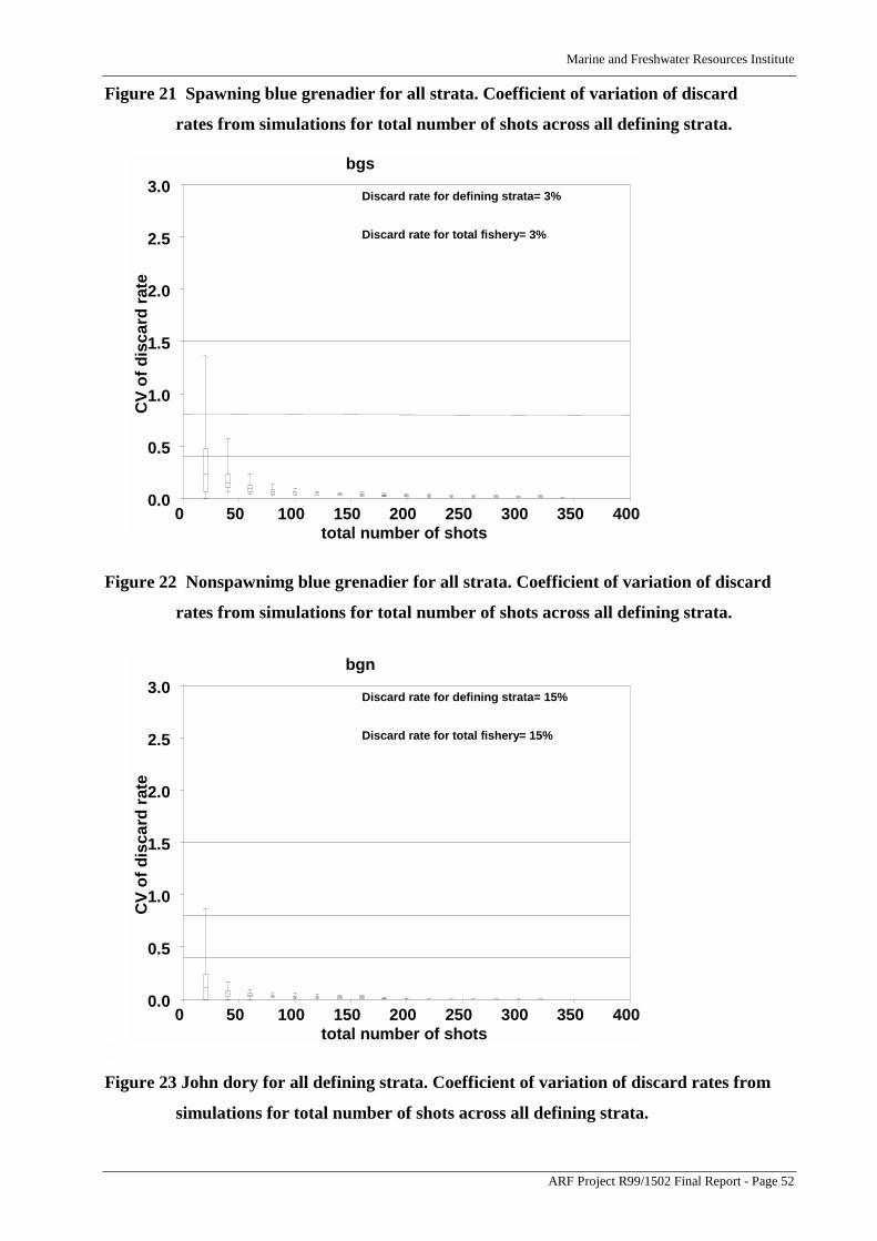
Marine and Freshwater Resources Institute
ARF Project R99/1502 Final Report - Page 52
Figure 21 Spawning blue grenadier for all strata. Coefficient of variation of discard
rates from simulations for total number of shots across all defining strata.
Figure 22 Nonspawnimg blue grenadier for all strata. Coefficient of variation of discard
rates from simulations for total number of shots across all defining strata.
Figure 23 John dory for all defining strata. Coefficient of variation of discard rates from
simulations for total number of shots across all defining strata.
Discard rate for defining strata= 15%
Discard rate for total fishery= 15%
bgn
CV
of d
isca
rd ra
te
0.0
0.5
1.0
1.5
2.0
2.5
3.0
total number of shots0 50 100 150 200 250 300 350 400
Discard rate for defining strata= 3%
Discard rate for total fishery= 3%
bgsC
V of
dis
card
rate
0.0
0.5
1.0
1.5
2.0
2.5
3.0
total number of shots0 50 100 150 200 250 300 350 400

Marine and Freshwater Resources Institute
ARF Project R99/1502 Final Report - Page 53
Figure 24 Mirror dory for all defining strata. Coefficient of variation of discard rates
from simulations for total number of shots across all defining strata.
Figure 25 Tiger flathead for all defining strata. Coefficient of variation of discard rates
from simulations for total number of shots across all defining strata.
Discard rate for defining strata= 2%
Discard rate for total fishery= 7%
dojC
V of
dis
card
rate
0.0
0.5
1.0
1.5
2.0
2.5
3.0
total number of shots0 50 100 150 200 250 300 350 400
Discard rate for defining strata= 48%
Discard rate for total fishery= 44%
dom
CV
of d
isca
rd ra
te
0.0
0.5
1.0
1.5
2.0
2.5
3.0
total number of shots0 50 100 150 200 250 300 350 400

Marine and Freshwater Resources Institute
ARF Project R99/1502 Final Report - Page 54
Figure 26 Eastern gemfish for all defining strata. Coefficient of variation of discard
rates from simulations for total number of shots across all defining strata.
Discard rate for defining strata= 8%
Discard rate for total fishery= 8%
flt
CV
of d
isca
rd ra
te
0.0
0.5
1.0
1.5
2.0
2.5
3.0
total number of shots0 50 100 150 200 250 300 350 400
Discard rate for defining strata= 14%
Discard rate for total fishery= 15%
gee
CV
of d
isca
rd ra
te
0.0
0.5
1.0
1.5
2.0
2.5
3.0
total number of shots0 50 100 150 200 250 300 350 400

Marine and Freshwater Resources Institute
ARF Project R99/1502 Final Report - Page 55
Figure 27 Western gemfish for all defining strata. Coefficient of variation of discard
rates from simulations for total number of shots across all defining strata.
Figure 28 Ling for all defining strata. Coefficient of variation of discard rates from
simulations for total number of shots across all defining strata.
Discard rate for defining strata= 1%
Discard rate for total fishery= 1%
lig
CV
of d
isca
rd ra
te
0.0
0.5
1.0
1.5
2.0
2.5
3.0
total number of shots0 50 100 150 200 250 300 350 400
Discard rate for defining strata= 4%
Discard rate for total fishery= 4%
gew
CV
of d
isca
rd ra
te
0.0
0.5
1.0
1.5
2.0
2.5
3.0
total number of shots0 50 100 150 200 250 300 350 400

Marine and Freshwater Resources Institute
ARF Project R99/1502 Final Report - Page 56
Figure 29 Morwong for all defining strata. Coefficient of variation of discard rates from
simulations for total number of shots across all defining strata.
Figure 30 Orange roughy for all defining strata. Coefficient of variation of discard rates
from simulations for total number of shots across all defining strata.
Discard rate for defining strata= 4%
Discard rate for total fishery= 4%
mow
CV
of d
isca
rd ra
te
0.0
0.5
1.0
1.5
2.0
2.5
3.0
total number of shots0 50 100 150 200 250 300 350 400
Discard rate for defining strata= 1%
Discard rate for total fishery= 1%
oro
CV
of d
isca
rd ra
te
0.0
0.5
1.0
1.5
2.0
2.5
3.0
total number of shots0 50 100 150 200 250 300 350 400

Marine and Freshwater Resources Institute
ARF Project R99/1502 Final Report - Page 57
Figure 31 All other species for all strata. Coefficient of variation of discard rates from
simulations for total number of shots across all defining strata.
Figure 32 Redfish for all defining strata. Coefficient of variation of discard rates from
simulations for total number of shots across all defining strata.
Discard rate for defining strata= 60%
Discard rate for total fishery= 53%
red
CV
of d
isca
rd ra
te
0.0
0.5
1.0
1.5
2.0
2.5
3.0
total number of shots0 50 100 150 200 250 300 350 400
Discard rate for defining strata= 59%
Discard rate for total fishery= 59%
oth
CV
of d
isca
rd ra
te
0.0
0.5
1.0
1.5
2.0
2.5
3.0
total number of shots0 50 100 150 200 250 300 350 400

Marine and Freshwater Resources Institute
ARF Project R99/1502 Final Report - Page 58
Figure 33 Inshore ocean perch for all strata. Coefficient of variation of discard rates
from simulations for total number of shots across all defining strata.
Figure 34 Offshore ocean perch for all strata. Coefficient of variation of discard rates
from simulations for total number of shots across all defining strata.
Discard rate for defining strata= 71%
Discard rate for total fishery= 72%
rei
CV
of d
isca
rd ra
te
0.0
0.5
1.0
1.5
2.0
2.5
3.0
total number of shots0 50 100 150 200 250 300 350 400
Discard rate for defining strata= 16%
Discard rate for total fishery= 17%
reo
CV
of d
isca
rd ra
te
0.0
0.5
1.0
1.5
2.0
2.5
3.0
total number of shots0 50 100 150 200 250 300 350 400
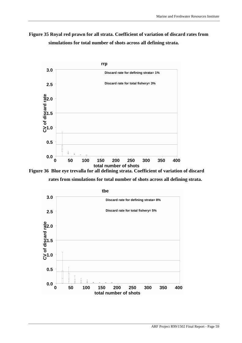
Marine and Freshwater Resources Institute
ARF Project R99/1502 Final Report - Page 59
Figure 35 Royal red prawn for all strata. Coefficient of variation of discard rates from
simulations for total number of shots across all defining strata.
Figure 36 Blue eye trevalla for all defining strata. Coefficient of variation of discard
rates from simulations for total number of shots across all defining strata.
Discard rate for defining strata= 1%
Discard rate for total fishery= 3%
rrp
CV
of d
isca
rd ra
te
0.0
0.5
1.0
1.5
2.0
2.5
3.0
total number of shots0 50 100 150 200 250 300 350 400
Discard rate for defining strata= 8%
Discard rate for total fishery= 5%
tbe
CV
of d
isca
rd ra
te
0.0
0.5
1.0
1.5
2.0
2.5
3.0
total number of shots0 50 100 150 200 250 300 350 400

Marine and Freshwater Resources Institute
ARF Project R99/1502 Final Report - Page 60
Figure 37 Silver trevally for all defining strata. Coefficient of variation of discard rates
from simulations for total number of shots across all defining strata.
Figure 38 Spotted warehou for all defining strata. Coefficient of variation of discard
rates from simulations for total number of shots across all defining strata.
Discard rate for defining strata= 0%
Discard rate for total fishery= 11%
tre
CV
of d
isca
rd ra
te
0.0
0.5
1.0
1.5
2.0
2.5
3.0
total number of shots0 50 100 150 200 250 300 350 400
Discard rate for defining strata= 25%
Discard rate for total fishery= 20%
trs
CV
of d
isca
rd ra
te
0.0
0.5
1.0
1.5
2.0
2.5
3.0
total number of shots0 50 100 150 200 250 300 350 400
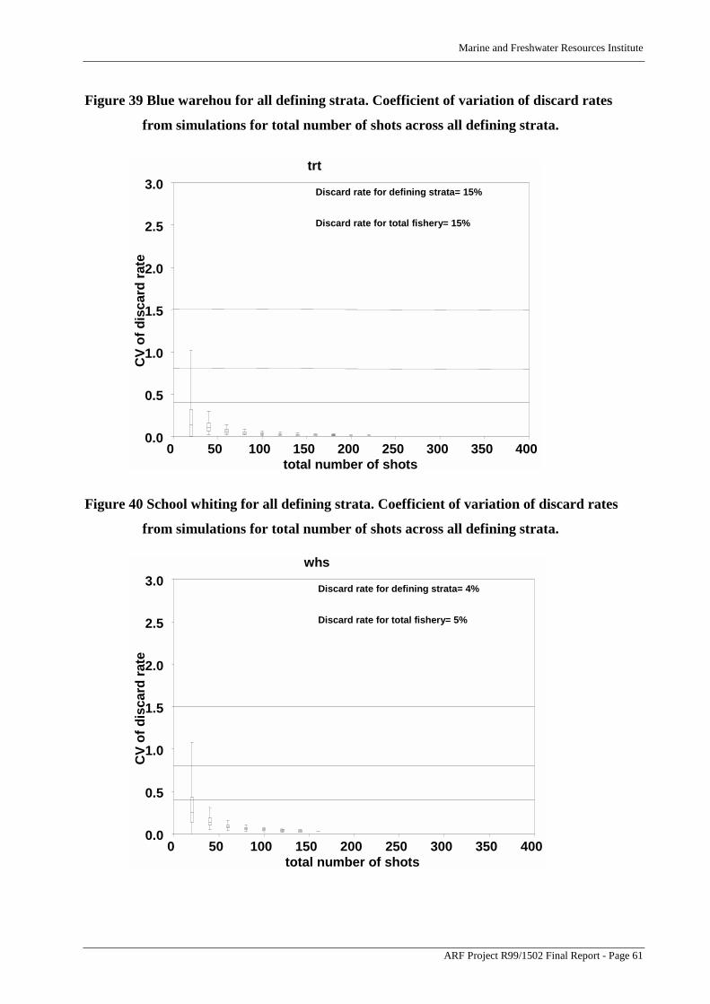
Marine and Freshwater Resources Institute
ARF Project R99/1502 Final Report - Page 61
Figure 39 Blue warehou for all defining strata. Coefficient of variation of discard rates
from simulations for total number of shots across all defining strata.
Figure 40 School whiting for all defining strata. Coefficient of variation of discard rates
from simulations for total number of shots across all defining strata.
Discard rate for defining strata= 4%
Discard rate for total fishery= 5%
whs
CV
of d
isca
rd ra
te
0.0
0.5
1.0
1.5
2.0
2.5
3.0
total number of shots0 50 100 150 200 250 300 350 400
Discard rate for defining strata= 15%
Discard rate for total fishery= 15%
trt
CV
of d
isca
rd ra
te
0.0
0.5
1.0
1.5
2.0
2.5
3.0
total number of shots0 50 100 150 200 250 300 350 400

Marine and Freshwater Resources Institute
ARF Project R99/1502 Final Report - Page 62
Figure 41 The mean weighted CV of length frequencies for each combination of sample
number and sample size (i.e. number of fish within each sample).
20 fish
40 fish
60 fish 80 fish100 fish140 fish200 fish
Blue Warehou
Mea
n w
eigh
ted
CV
0.0
0.1
0.2
0.3
Number of Samples25 50 75 100 125 150 175 200
20 fish
40 fish
60 fish
80 fish100 fish140 fish200 fish
Blue eye Trevalla
Mea
n w
eigh
ted
CV
0.0
0.1
0.2
0.3
Number of Samples25 50 75 100 125 150 175 200

Marine and Freshwater Resources Institute
ARF Project R99/1502 Final Report - Page 63
20 fish
40 fish
60 fish
80 fish100 fish
140 fish200 fish
Blue grenadier - spawning M
ean
wei
ghte
d C
V
0.0
0.1
0.2
0.3
Number of Samples25 50 75 100 125 150 175 200
20 fish
40 fish
60 fish
80 fish
100 fish
140 fish200 fish
Eastern Gemfish
Mea
n w
eigh
ted
CV
0.0
0.1
0.2
0.3
Number of Samples25 50 75 100 125 150 175 200

Marine and Freshwater Resources Institute
ARF Project R99/1502 Final Report - Page 64
20 fish
40 fish
60 fish 80 fish100 fish140 fish200 fish
Jackass morwong M
ean
wei
ghte
d C
V
0.0
0.1
0.2
0.3
Number of Samples25 50 75 100 125 150 175 200
20 fish
40 fish
60 fish
80 fish100 fish140 fish200 fish
John dory
Mea
n w
eigh
ted
CV
0.0
0.1
0.2
0.3
Number of Samples25 50 75 100 125 150 175 200

Marine and Freshwater Resources Institute
ARF Project R99/1502 Final Report - Page 65
20 fish
40 fish
60 fish
80 fish
100 fish
140 fish200 fish
Mirror dory M
ean
wei
ghte
d C
V
0.0
0.1
0.2
0.3
Number of Samples25 50 75 100 125 150 175 200
20 fish 40 fish
60 fish
80 fish
100 fish
140 fish
200 fish
Ocean perch - inshore
Mea
n w
eigh
ted
CV
0.0
0.1
0.2
0.3
Number of Samples25 50 75 100 125 150 175 200

Marine and Freshwater Resources Institute
ARF Project R99/1502 Final Report - Page 66
20 fish
40 fish
60 fish
80 fish100 fish
140 fish200 fish
Ocean perch - offshore M
ean
wei
ghte
d C
V
0.0
0.1
0.2
0.3
Number of Samples25 50 75 100 125 150 175 200
20 fish
40 fish
60 fish 80 fish100 fish140 fish200 fish
Orange Roughy
Mea
n w
eigh
ted
CV
0.0
0.1
0.2
0.3
Number of Samples25 50 75 100 125 150 175 200

Marine and Freshwater Resources Institute
ARF Project R99/1502 Final Report - Page 67
20 fish
40 fish
60 fish
80 fish100 fish140 fish200 fish
Pink Ling M
ean
wei
ghte
d C
V
0.0
0.1
0.2
0.3
Number of Samples25 50 75 100 125 150 175 200
20 fish
40 fish
60 fish
80 fish100 fish140 fish200 fish
Redfish
Mea
n w
eigh
ted
CV
0.0
0.1
0.2
0.3
Number of Samples25 50 75 100 125 150 175 200

Marine and Freshwater Resources Institute
ARF Project R99/1502 Final Report - Page 68
20 fish 40 fish
60 fish
80 fish
100 fish
140 fish
200 fish
Royal red prawn M
ean
wei
ghte
d C
V
0.0
0.1
0.2
0.3
Number of Samples25 50 75 100 125 150 175 200
20 fish
40 fish
60 fish
80 fish100 fish140 fish200 fish
School whiting
Mea
n w
eigh
ted
CV
0.0
0.1
0.2
0.3
Number of Samples25 50 75 100 125 150 175 200

Marine and Freshwater Resources Institute
ARF Project R99/1502 Final Report - Page 69
20 fish 40 fish
60 fish
80 fish
100 fish
140 fish
200 fish
Silver trevally M
ean
wei
ghte
d C
V
0.0
0.1
0.2
0.3
Number of Samples25 50 75 100 125 150 175 200
20 fish
40 fish
60 fish 80 fish100 fish140 fish200 fish
Spotted warehou
Mea
n w
eigh
ted
CV
0.0
0.1
0.2
0.3
Number of Samples25 50 75 100 125 150 175 200

Marine and Freshwater Resources Institute
ARF Project R99/1502 Final Report - Page 70
20 fish
40 fish
60 fish 80 fish100 fish140 fish200 fish
Tiger flathead M
ean
wei
ghte
d C
V
0.0
0.1
0.2
0.3
Number of Samples25 50 75 100 125 150 175 200
20 fish
40 fish
60 fish 80 fish100 fish140 fish200 fish
Western Gemfish
Mea
n w
eigh
ted
CV
0.0
0.1
0.2
0.3
Number of Samples25 50 75 100 125 150 175 200