R09 - Two-way ANOVA - jarad.me · Two-way ANOVA Data An experiment was run on tomato plants to...
118
R09 - Two-way ANOVA STAT 587 (Engineering) - Iowa State University April 26, 2019 (STAT587@ISU) R09 - Two-way ANOVA April 26, 2019 1 / 49
Transcript of R09 - Two-way ANOVA - jarad.me · Two-way ANOVA Data An experiment was run on tomato plants to...

R09 - Two-way ANOVA
STAT 587 (Engineering) - Iowa State University
April 26, 2019
(STAT587@ISU) R09 - Two-way ANOVA April 26, 2019 1 / 49
Two factors
Consider the question of the affect of variety and density on yield undervarious experimental designs:
Balanced, complete design
Unbalanced, complete
Incomplete
We will also consider the problem of finding the density that maximizesyield.
(STAT587@ISU) R09 - Two-way ANOVA April 26, 2019 2 / 49
Two-way ANOVA
Data
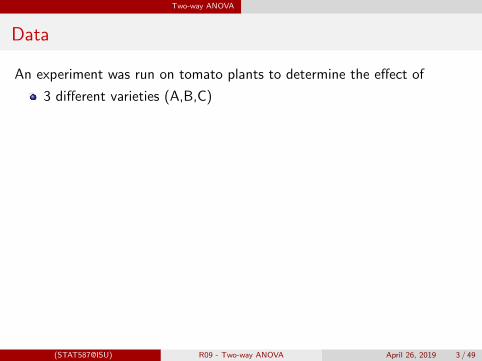
An experiment was run on tomato plants to determine the effect of
3 different varieties (A,B,C)
and
4 different planting densities (10,20,30,40)
on yield.
There is an expectation that planting density will have a different effectdepending on the variety. Therefore a balanced, complete, randomizeddesign was used.
complete: each treatment (variety × density) is represented in theexperiment
balanced: each treatment in the experiment has the same number ofreplications
randomized: treatment was randomly assigned to the plot
This is also referred to as a full factorial or fully crossed design.
(STAT587@ISU) R09 - Two-way ANOVA April 26, 2019 3 / 49
Two-way ANOVA
Data
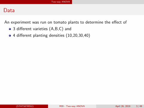
An experiment was run on tomato plants to determine the effect of
3 different varieties (A,B,C) and
4 different planting densities (10,20,30,40)
on yield.
There is an expectation that planting density will have a different effectdepending on the variety. Therefore a balanced, complete, randomizeddesign was used.
complete: each treatment (variety × density) is represented in theexperiment
balanced: each treatment in the experiment has the same number ofreplications
randomized: treatment was randomly assigned to the plot
This is also referred to as a full factorial or fully crossed design.
(STAT587@ISU) R09 - Two-way ANOVA April 26, 2019 3 / 49

Two-way ANOVA
Data
An experiment was run on tomato plants to determine the effect of
3 different varieties (A,B,C) and
4 different planting densities (10,20,30,40)
on yield.
There is an expectation that planting density will have a different effectdepending on the variety.
Therefore a balanced, complete, randomizeddesign was used.
complete: each treatment (variety × density) is represented in theexperiment
balanced: each treatment in the experiment has the same number ofreplications
randomized: treatment was randomly assigned to the plot
This is also referred to as a full factorial or fully crossed design.
(STAT587@ISU) R09 - Two-way ANOVA April 26, 2019 3 / 49

Two-way ANOVA
Data
An experiment was run on tomato plants to determine the effect of
3 different varieties (A,B,C) and
4 different planting densities (10,20,30,40)
on yield.
There is an expectation that planting density will have a different effectdepending on the variety. Therefore a balanced, complete, randomizeddesign was used.
complete: each treatment (variety × density) is represented in theexperiment
balanced: each treatment in the experiment has the same number ofreplications
randomized: treatment was randomly assigned to the plot
This is also referred to as a full factorial or fully crossed design.
(STAT587@ISU) R09 - Two-way ANOVA April 26, 2019 3 / 49

Two-way ANOVA
Data
An experiment was run on tomato plants to determine the effect of
3 different varieties (A,B,C) and
4 different planting densities (10,20,30,40)
on yield.
There is an expectation that planting density will have a different effectdepending on the variety. Therefore a balanced, complete, randomizeddesign was used.
complete: each treatment (variety × density) is represented in theexperiment
balanced: each treatment in the experiment has the same number ofreplications
randomized: treatment was randomly assigned to the plot
This is also referred to as a full factorial or fully crossed design.
(STAT587@ISU) R09 - Two-way ANOVA April 26, 2019 3 / 49

Two-way ANOVA
Hypotheses
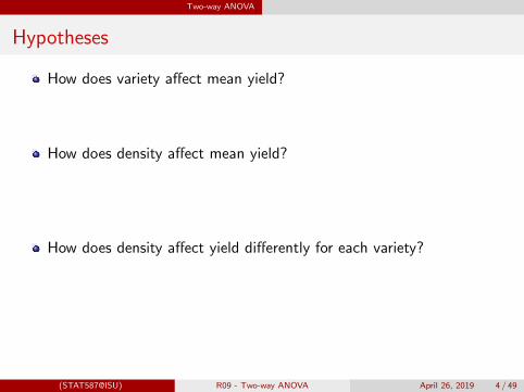
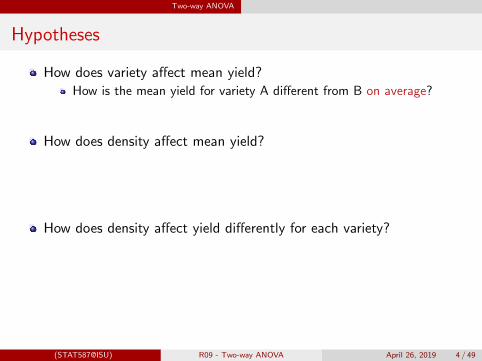
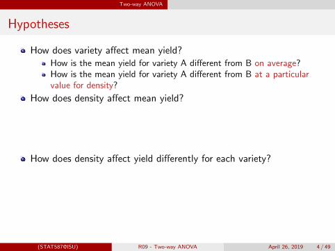
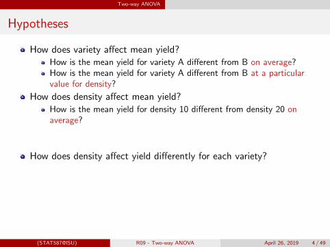
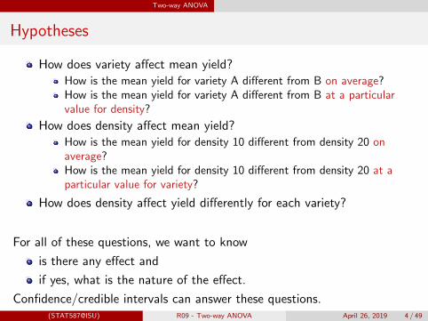
How does variety affect mean yield?
How is the mean yield for variety A different from B on average?How is the mean yield for variety A different from B at a particularvalue for density?
How does density affect mean yield?
How is the mean yield for density 10 different from density 20 onaverage?How is the mean yield for density 10 different from density 20 at aparticular value for variety?
How does density affect yield differently for each variety?
For all of these questions, we want to know
is there any effect and
if yes, what is the nature of the effect.
Confidence/credible intervals can answer these questions.
(STAT587@ISU) R09 - Two-way ANOVA April 26, 2019 4 / 49

Two-way ANOVA
Hypotheses
How does variety affect mean yield?
How is the mean yield for variety A different from B on average?How is the mean yield for variety A different from B at a particularvalue for density?
How does density affect mean yield?
How is the mean yield for density 10 different from density 20 onaverage?How is the mean yield for density 10 different from density 20 at aparticular value for variety?
How does density affect yield differently for each variety?
For all of these questions, we want to know
is there any effect and
if yes, what is the nature of the effect.
Confidence/credible intervals can answer these questions.
(STAT587@ISU) R09 - Two-way ANOVA April 26, 2019 4 / 49
Two-way ANOVA
Hypotheses
How does variety affect mean yield?How is the mean yield for variety A different from B on average?
How is the mean yield for variety A different from B at a particularvalue for density?
How does density affect mean yield?
How is the mean yield for density 10 different from density 20 onaverage?How is the mean yield for density 10 different from density 20 at aparticular value for variety?
How does density affect yield differently for each variety?
For all of these questions, we want to know
is there any effect and
if yes, what is the nature of the effect.
Confidence/credible intervals can answer these questions.
(STAT587@ISU) R09 - Two-way ANOVA April 26, 2019 4 / 49
Two-way ANOVA
Hypotheses
How does variety affect mean yield?How is the mean yield for variety A different from B on average?How is the mean yield for variety A different from B at a particularvalue for density?
How does density affect mean yield?How is the mean yield for density 10 different from density 20 onaverage?
How is the mean yield for density 10 different from density 20 at aparticular value for variety?
How does density affect yield differently for each variety?
For all of these questions, we want to know
is there any effect and
if yes, what is the nature of the effect.
Confidence/credible intervals can answer these questions.
(STAT587@ISU) R09 - Two-way ANOVA April 26, 2019 4 / 49

Two-way ANOVA
Hypotheses
How does variety affect mean yield?How is the mean yield for variety A different from B on average?How is the mean yield for variety A different from B at a particularvalue for density?
How does density affect mean yield?How is the mean yield for density 10 different from density 20 onaverage?How is the mean yield for density 10 different from density 20 at aparticular value for variety?
How does density affect yield differently for each variety?
For all of these questions, we want to know
is there any effect and
if yes, what is the nature of the effect.
Confidence/credible intervals can answer these questions.
(STAT587@ISU) R09 - Two-way ANOVA April 26, 2019 4 / 49
Two-way ANOVA
Hypotheses
How does variety affect mean yield?How is the mean yield for variety A different from B on average?How is the mean yield for variety A different from B at a particularvalue for density?
How does density affect mean yield?How is the mean yield for density 10 different from density 20 onaverage?How is the mean yield for density 10 different from density 20 at aparticular value for variety?
How does density affect yield differently for each variety?
For all of these questions, we want to know
is there any effect and
if yes, what is the nature of the effect.
Confidence/credible intervals can answer these questions.(STAT587@ISU) R09 - Two-way ANOVA April 26, 2019 4 / 49

Two-way ANOVA
8
12
16
20
10 20 30 40
Density
Yie
ld
Variety
C
A
B
(STAT587@ISU) R09 - Two-way ANOVA April 26, 2019 5 / 49
Two-way ANOVA
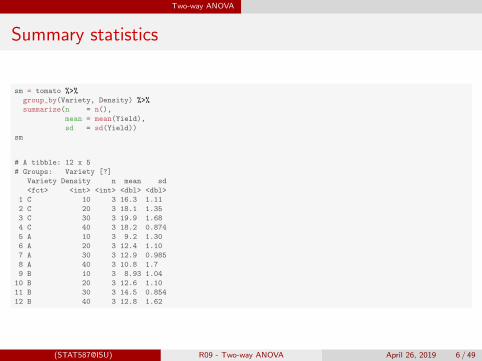
Summary statistics
sm = tomato %>%
group_by(Variety, Density) %>%
summarize(n = n(),
mean = mean(Yield),
sd = sd(Yield))
sm
# A tibble: 12 x 5
# Groups: Variety [?]
Variety Density n mean sd
<fct> <int> <int> <dbl> <dbl>
1 C 10 3 16.3 1.11
2 C 20 3 18.1 1.35
3 C 30 3 19.9 1.68
4 C 40 3 18.2 0.874
5 A 10 3 9.2 1.30
6 A 20 3 12.4 1.10
7 A 30 3 12.9 0.985
8 A 40 3 10.8 1.7
9 B 10 3 8.93 1.04
10 B 20 3 12.6 1.10
11 B 30 3 14.5 0.854
12 B 40 3 12.8 1.62
(STAT587@ISU) R09 - Two-way ANOVA April 26, 2019 6 / 49
Two-way ANOVA
Two-way ANOVA
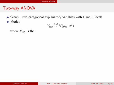
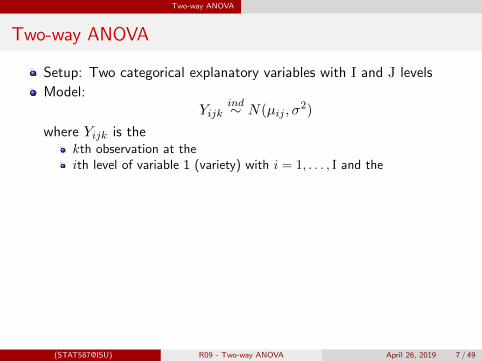
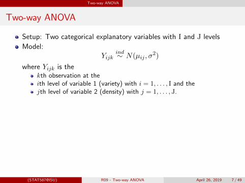
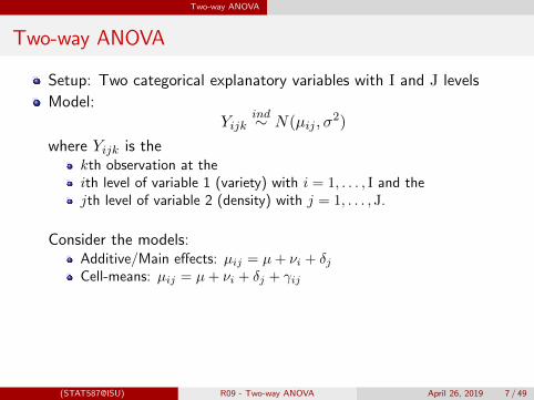
Setup: Two categorical explanatory variables with I and J levels
Model:Yijk
ind∼ N(µij , σ2)
where Yijk is the
kth observation at theith level of variable 1 (variety) with i = 1, . . . , I and thejth level of variable 2 (density) with j = 1, . . . , J.
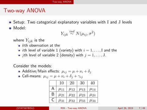
Consider the models:
Additive/Main effects: µij = µ+ νi + δjCell-means: µij = µ+ νi + δj + γij
10 20 30 40
A µ11 µ12 µ13 µ14B µ21 µ22 µ23 µ24C µ31 µ32 µ33 µ34
(STAT587@ISU) R09 - Two-way ANOVA April 26, 2019 7 / 49
Two-way ANOVA
Two-way ANOVA
Setup: Two categorical explanatory variables with I and J levels
Model:Yijk
ind∼ N(µij , σ2)
where Yijk is the
kth observation at theith level of variable 1 (variety) with i = 1, . . . , I and thejth level of variable 2 (density) with j = 1, . . . , J.
Consider the models:
Additive/Main effects: µij = µ+ νi + δjCell-means: µij = µ+ νi + δj + γij
10 20 30 40
A µ11 µ12 µ13 µ14B µ21 µ22 µ23 µ24C µ31 µ32 µ33 µ34
(STAT587@ISU) R09 - Two-way ANOVA April 26, 2019 7 / 49

Two-way ANOVA
Two-way ANOVA
Setup: Two categorical explanatory variables with I and J levels
Model:Yijk
ind∼ N(µij , σ2)
where Yijk is thekth observation at the
ith level of variable 1 (variety) with i = 1, . . . , I and thejth level of variable 2 (density) with j = 1, . . . , J.
Consider the models:
Additive/Main effects: µij = µ+ νi + δjCell-means: µij = µ+ νi + δj + γij
10 20 30 40
A µ11 µ12 µ13 µ14B µ21 µ22 µ23 µ24C µ31 µ32 µ33 µ34
(STAT587@ISU) R09 - Two-way ANOVA April 26, 2019 7 / 49
Two-way ANOVA
Two-way ANOVA
Setup: Two categorical explanatory variables with I and J levels
Model:Yijk
ind∼ N(µij , σ2)
where Yijk is thekth observation at theith level of variable 1 (variety) with i = 1, . . . , I and the
jth level of variable 2 (density) with j = 1, . . . , J.
Consider the models:
Additive/Main effects: µij = µ+ νi + δjCell-means: µij = µ+ νi + δj + γij
10 20 30 40
A µ11 µ12 µ13 µ14B µ21 µ22 µ23 µ24C µ31 µ32 µ33 µ34
(STAT587@ISU) R09 - Two-way ANOVA April 26, 2019 7 / 49

Two-way ANOVA
Two-way ANOVA
Setup: Two categorical explanatory variables with I and J levels
Model:Yijk
ind∼ N(µij , σ2)
where Yijk is thekth observation at theith level of variable 1 (variety) with i = 1, . . . , I and thejth level of variable 2 (density) with j = 1, . . . , J.
Consider the models:
Additive/Main effects: µij = µ+ νi + δjCell-means: µij = µ+ νi + δj + γij
10 20 30 40
A µ11 µ12 µ13 µ14B µ21 µ22 µ23 µ24C µ31 µ32 µ33 µ34
(STAT587@ISU) R09 - Two-way ANOVA April 26, 2019 7 / 49
Two-way ANOVA
Two-way ANOVA
Setup: Two categorical explanatory variables with I and J levels
Model:Yijk
ind∼ N(µij , σ2)
where Yijk is thekth observation at theith level of variable 1 (variety) with i = 1, . . . , I and thejth level of variable 2 (density) with j = 1, . . . , J.
Consider the models:
Additive/Main effects: µij = µ+ νi + δjCell-means: µij = µ+ νi + δj + γij
10 20 30 40
A µ11 µ12 µ13 µ14B µ21 µ22 µ23 µ24C µ31 µ32 µ33 µ34
(STAT587@ISU) R09 - Two-way ANOVA April 26, 2019 7 / 49

Two-way ANOVA
Two-way ANOVA
Setup: Two categorical explanatory variables with I and J levels
Model:Yijk
ind∼ N(µij , σ2)
where Yijk is thekth observation at theith level of variable 1 (variety) with i = 1, . . . , I and thejth level of variable 2 (density) with j = 1, . . . , J.
Consider the models:Additive/Main effects: µij = µ+ νi + δj
Cell-means: µij = µ+ νi + δj + γij
10 20 30 40
A µ11 µ12 µ13 µ14B µ21 µ22 µ23 µ24C µ31 µ32 µ33 µ34
(STAT587@ISU) R09 - Two-way ANOVA April 26, 2019 7 / 49

Two-way ANOVA
Two-way ANOVA
Setup: Two categorical explanatory variables with I and J levels
Model:Yijk
ind∼ N(µij , σ2)
where Yijk is thekth observation at theith level of variable 1 (variety) with i = 1, . . . , I and thejth level of variable 2 (density) with j = 1, . . . , J.
Consider the models:Additive/Main effects: µij = µ+ νi + δjCell-means: µij = µ+ νi + δj + γij
10 20 30 40
A µ11 µ12 µ13 µ14B µ21 µ22 µ23 µ24C µ31 µ32 µ33 µ34
(STAT587@ISU) R09 - Two-way ANOVA April 26, 2019 7 / 49
Two-way ANOVA
Two-way ANOVA
Setup: Two categorical explanatory variables with I and J levels
Model:Yijk
ind∼ N(µij , σ2)
where Yijk is thekth observation at theith level of variable 1 (variety) with i = 1, . . . , I and thejth level of variable 2 (density) with j = 1, . . . , J.
Consider the models:Additive/Main effects: µij = µ+ νi + δjCell-means: µij = µ+ νi + δj + γij
10 20 30 40
A µ11 µ12 µ13 µ14B µ21 µ22 µ23 µ24C µ31 µ32 µ33 µ34
(STAT587@ISU) R09 - Two-way ANOVA April 26, 2019 7 / 49

Two-way ANOVA
As a regression model
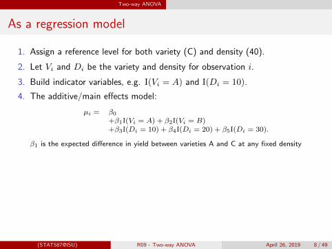
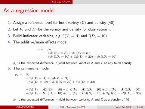
1. Assign a reference level for both variety (C) and density (40).
2. Let Vi and Di be the variety and density for observation i.
3. Build indicator variables, e.g. I(Vi = A) and I(Di = 10).
4. The additive/main effects model:
µi = β0+β1I(Vi = A) + β2I(Vi = B)+β3I(Di = 10) + β4I(Di = 20) + β5I(Di = 30).
β1 is the expected difference in yield between varieties A and C at any fixed density
5. The cell-means model:
µi = β0+β1I(Vi = A) + β2I(Vi = B)+β3I(Di = 10) + β4I(Di = 20) + β5I(Di = 30)
+β6I(Vi = A)I(Di = 10) + β 7I(Vi = A)I(Di = 20) + β 8I(Vi = A)I(Di = 30)+β9I(Vi = B)I(Di = 10) + β10I(Vi = B)I(Di = 20) + β11I(Vi = B)I(Di = 30)
β1 is the expected difference in yield between varieties A and C at a density of 40
(STAT587@ISU) R09 - Two-way ANOVA April 26, 2019 8 / 49

Two-way ANOVA
As a regression model
1. Assign a reference level for both variety (C) and density (40).
2. Let Vi and Di be the variety and density for observation i.
3. Build indicator variables, e.g. I(Vi = A) and I(Di = 10).
4. The additive/main effects model:
µi = β0+β1I(Vi = A) + β2I(Vi = B)+β3I(Di = 10) + β4I(Di = 20) + β5I(Di = 30).
β1 is the expected difference in yield between varieties A and C at any fixed density
5. The cell-means model:
µi = β0+β1I(Vi = A) + β2I(Vi = B)+β3I(Di = 10) + β4I(Di = 20) + β5I(Di = 30)
+β6I(Vi = A)I(Di = 10) + β 7I(Vi = A)I(Di = 20) + β 8I(Vi = A)I(Di = 30)+β9I(Vi = B)I(Di = 10) + β10I(Vi = B)I(Di = 20) + β11I(Vi = B)I(Di = 30)
β1 is the expected difference in yield between varieties A and C at a density of 40
(STAT587@ISU) R09 - Two-way ANOVA April 26, 2019 8 / 49
Two-way ANOVA ANOVA Table
ANOVA Table
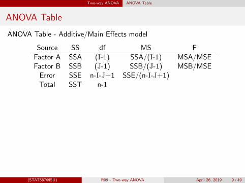
ANOVA Table - Additive/Main Effects model
Source SS df MS F
Factor A SSA (I-1) SSA/(I-1) MSA/MSEFactor B SSB (J-1) SSB/(J-1) MSB/MSE
Error SSE n-I-J+1 SSE/(n-I-J+1)Total SST n-1
ANOVA Table - Cell-means model
Source SS df MS
Factor A SSA I-1 SSA/(I-1) MSA/MSEFactor B SSB J-1 SSB/(J-1) MSB/MSE
Interaction AB SSAB (I-1)(J-1) SSAB /(I-1)(J-1) MSAB/MSEError SSE n-IJ SSE/(n-IJ)Total SST n-1
(STAT587@ISU) R09 - Two-way ANOVA April 26, 2019 9 / 49

Two-way ANOVA ANOVA Table
ANOVA Table
ANOVA Table - Additive/Main Effects model
Source SS df MS F
Factor A SSA (I-1) SSA/(I-1) MSA/MSEFactor B SSB (J-1) SSB/(J-1) MSB/MSE
Error SSE n-I-J+1 SSE/(n-I-J+1)Total SST n-1
ANOVA Table - Cell-means model
Source SS df MS
Factor A SSA I-1 SSA/(I-1) MSA/MSEFactor B SSB J-1 SSB/(J-1) MSB/MSE
Interaction AB SSAB (I-1)(J-1) SSAB /(I-1)(J-1) MSAB/MSEError SSE n-IJ SSE/(n-IJ)Total SST n-1
(STAT587@ISU) R09 - Two-way ANOVA April 26, 2019 9 / 49
Two-way ANOVA ANOVA Table
Two-way ANOVA in R
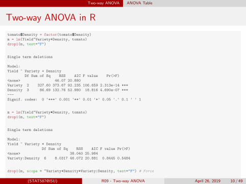
tomato$Density = factor(tomato$Density)
m = lm(Yield~Variety+Density, tomato)
drop1(m, test="F")
Single term deletions
Model:
Yield ~ Variety + Density
Df Sum of Sq RSS AIC F value Pr(>F)
<none> 46.07 20.880
Variety 2 327.60 373.67 92.235 106.659 2.313e-14 ***
Density 3 86.69 132.76 52.980 18.816 4.690e-07 ***
---
Signif. codes: 0 '***' 0.001 '**' 0.01 '*' 0.05 '.' 0.1 ' ' 1
m = lm(Yield~Variety*Density, tomato)
drop1(m, test="F")
Single term deletions
Model:
Yield ~ Variety * Density
Df Sum of Sq RSS AIC F value Pr(>F)
<none> 38.040 25.984
Variety:Density 6 8.0317 46.072 20.881 0.8445 0.5484
drop1(m, scope = ~Variety+Density+Variety:Density, test="F") # Force
Single term deletions
Model:
Yield ~ Variety * Density
Df Sum of Sq RSS AIC F value Pr(>F)
<none> 38.040 25.984
Variety 2 104.749 142.789 69.603 33.0438 1.278e-07 ***
Density 3 19.809 57.849 35.076 4.1660 0.01648 *
Variety:Density 6 8.032 46.072 20.880 0.8445 0.54836
---
Signif. codes: 0 '***' 0.001 '**' 0.01 '*' 0.05 '.' 0.1 ' ' 1
(STAT587@ISU) R09 - Two-way ANOVA April 26, 2019 10 / 49

Two-way ANOVA Additive vs cell-means
Additive vs cell-means
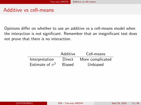
Opinions differ on whether to use an additive vs a cell-means model whenthe interaction is not significant.
Remember that an insignificant test doesnot prove that there is no interaction.
Additive Cell-means
Interpretation Direct More complicatedEstimate of σ2 Biased Unbiased
We will continue using the cell-means model to answer the scientificquestions of interest.
(STAT587@ISU) R09 - Two-way ANOVA April 26, 2019 11 / 49

Two-way ANOVA Additive vs cell-means
Additive vs cell-means
Opinions differ on whether to use an additive vs a cell-means model whenthe interaction is not significant. Remember that an insignificant test doesnot prove that there is no interaction.
Additive Cell-means
Interpretation Direct More complicatedEstimate of σ2 Biased Unbiased
We will continue using the cell-means model to answer the scientificquestions of interest.
(STAT587@ISU) R09 - Two-way ANOVA April 26, 2019 11 / 49

Two-way ANOVA Additive vs cell-means
ggplot(sm, aes(x=Density, y=mean, col=Variety)) + geom_line() + labs(y="Mean Yield") + theme_bw()
9
12
15
18
10 20 30 40
Density
Mea
n Y
ield Variety
C
A
B
(STAT587@ISU) R09 - Two-way ANOVA April 26, 2019 12 / 49
Two-way ANOVA Analysis in R
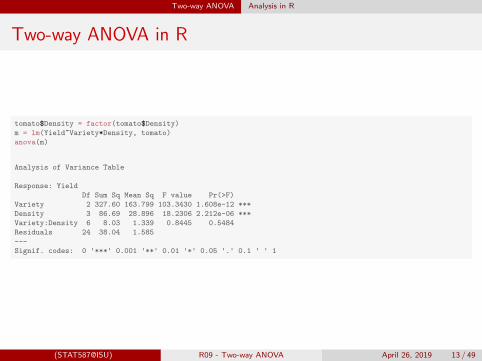
Two-way ANOVA in R
tomato$Density = factor(tomato$Density)
m = lm(Yield~Variety*Density, tomato)
anova(m)
Analysis of Variance Table
Response: Yield
Df Sum Sq Mean Sq F value Pr(>F)
Variety 2 327.60 163.799 103.3430 1.608e-12 ***
Density 3 86.69 28.896 18.2306 2.212e-06 ***
Variety:Density 6 8.03 1.339 0.8445 0.5484
Residuals 24 38.04 1.585
---
Signif. codes: 0 '***' 0.001 '**' 0.01 '*' 0.05 '.' 0.1 ' ' 1
(STAT587@ISU) R09 - Two-way ANOVA April 26, 2019 13 / 49
Two-way ANOVA Analysis in R
Variety comparison
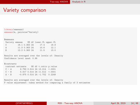
library(emmeans)
emmeans(m, pairwise~Variety)
$emmeans
Variety emmean SE df lower.CL upper.CL
C 18.1 0.363 24 17.4 18.9
A 11.3 0.363 24 10.6 12.1
B 12.2 0.363 24 11.5 13.0
Results are averaged over the levels of: Density
Confidence level used: 0.95
$contrasts
contrast estimate SE df t.ratio p.value
C - A 6.792 0.514 24 13.214 <.0001
C - B 5.917 0.514 24 11.512 <.0001
A - B -0.875 0.514 24 -1.702 0.2249
Results are averaged over the levels of: Density
P value adjustment: tukey method for comparing a family of 3 estimates
(STAT587@ISU) R09 - Two-way ANOVA April 26, 2019 14 / 49
Two-way ANOVA Analysis in R
Density comparison
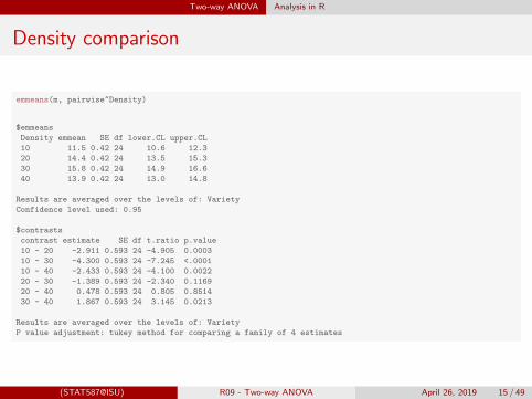
emmeans(m, pairwise~Density)
$emmeans
Density emmean SE df lower.CL upper.CL
10 11.5 0.42 24 10.6 12.3
20 14.4 0.42 24 13.5 15.3
30 15.8 0.42 24 14.9 16.6
40 13.9 0.42 24 13.0 14.8
Results are averaged over the levels of: Variety
Confidence level used: 0.95
$contrasts
contrast estimate SE df t.ratio p.value
10 - 20 -2.911 0.593 24 -4.905 0.0003
10 - 30 -4.300 0.593 24 -7.245 <.0001
10 - 40 -2.433 0.593 24 -4.100 0.0022
20 - 30 -1.389 0.593 24 -2.340 0.1169
20 - 40 0.478 0.593 24 0.805 0.8514
30 - 40 1.867 0.593 24 3.145 0.0213
Results are averaged over the levels of: Variety
P value adjustment: tukey method for comparing a family of 4 estimates
(STAT587@ISU) R09 - Two-way ANOVA April 26, 2019 15 / 49

Two-way ANOVA Analysis in R
emmeans(m, pairwise~Variety*Density)
$emmeans
Variety Density emmean SE df lower.CL upper.CL
C 10 16.30 0.727 24 14.80 17.8
A 10 9.20 0.727 24 7.70 10.7
B 10 8.93 0.727 24 7.43 10.4
C 20 18.10 0.727 24 16.60 19.6
A 20 12.43 0.727 24 10.93 13.9
B 20 12.63 0.727 24 11.13 14.1
C 30 19.93 0.727 24 18.43 21.4
A 30 12.90 0.727 24 11.40 14.4
B 30 14.50 0.727 24 13.00 16.0
C 40 18.17 0.727 24 16.67 19.7
A 40 10.80 0.727 24 9.30 12.3
B 40 12.77 0.727 24 11.27 14.3
Confidence level used: 0.95
$contrasts
contrast estimate SE df t.ratio p.value
C,10 - A,10 7.1000 1.03 24 6.907 <.0001
C,10 - B,10 7.3667 1.03 24 7.166 <.0001
C,10 - C,20 -1.8000 1.03 24 -1.751 0.8276
C,10 - A,20 3.8667 1.03 24 3.762 0.0356
C,10 - B,20 3.6667 1.03 24 3.567 0.0543
C,10 - C,30 -3.6333 1.03 24 -3.535 0.0582
C,10 - A,30 3.4000 1.03 24 3.308 0.0932
C,10 - B,30 1.8000 1.03 24 1.751 0.8276
C,10 - C,40 -1.8667 1.03 24 -1.816 0.7947
C,10 - A,40 5.5000 1.03 24 5.350 0.0008
C,10 - B,40 3.5333 1.03 24 3.437 0.0714
A,10 - B,10 0.2667 1.03 24 0.259 1.0000
A,10 - C,20 -8.9000 1.03 24 -8.658 <.0001
A,10 - A,20 -3.2333 1.03 24 -3.145 0.1284
A,10 - B,20 -3.4333 1.03 24 -3.340 0.0873
A,10 - C,30 -10.7333 1.03 24 -10.442 <.0001
A,10 - A,30 -3.7000 1.03 24 -3.599 0.0507
A,10 - B,30 -5.3000 1.03 24 -5.156 0.0013
A,10 - C,40 -8.9667 1.03 24 -8.723 <.0001
A,10 - A,40 -1.6000 1.03 24 -1.557 0.9085
A,10 - B,40 -3.5667 1.03 24 -3.470 0.0668
B,10 - C,20 -9.1667 1.03 24 -8.917 <.0001
B,10 - A,20 -3.5000 1.03 24 -3.405 0.0764
B,10 - B,20 -3.7000 1.03 24 -3.599 0.0507
B,10 - C,30 -11.0000 1.03 24 -10.701 <.0001
B,10 - A,30 -3.9667 1.03 24 -3.859 0.0287
B,10 - B,30 -5.5667 1.03 24 -5.415 0.0007
B,10 - C,40 -9.2333 1.03 24 -8.982 <.0001
B,10 - A,40 -1.8667 1.03 24 -1.816 0.7947
B,10 - B,40 -3.8333 1.03 24 -3.729 0.0382
C,20 - A,20 5.6667 1.03 24 5.513 0.0006
C,20 - B,20 5.4667 1.03 24 5.318 0.0009
C,20 - C,30 -1.8333 1.03 24 -1.783 0.8114
C,20 - A,30 5.2000 1.03 24 5.059 0.0017
C,20 - B,30 3.6000 1.03 24 3.502 0.0624
C,20 - C,40 -0.0667 1.03 24 -0.065 1.0000
C,20 - A,40 7.3000 1.03 24 7.102 <.0001
C,20 - B,40 5.3333 1.03 24 5.188 0.0012
A,20 - B,20 -0.2000 1.03 24 -0.195 1.0000
A,20 - C,30 -7.5000 1.03 24 -7.296 <.0001
A,20 - A,30 -0.4667 1.03 24 -0.454 1.0000
A,20 - B,30 -2.0667 1.03 24 -2.010 0.6829
A,20 - C,40 -5.7333 1.03 24 -5.577 0.0005
A,20 - A,40 1.6333 1.03 24 1.589 0.8970
A,20 - B,40 -0.3333 1.03 24 -0.324 1.0000
B,20 - C,30 -7.3000 1.03 24 -7.102 <.0001
B,20 - A,30 -0.2667 1.03 24 -0.259 1.0000
B,20 - B,30 -1.8667 1.03 24 -1.816 0.7947
B,20 - C,40 -5.5333 1.03 24 -5.383 0.0008
B,20 - A,40 1.8333 1.03 24 1.783 0.8114
B,20 - B,40 -0.1333 1.03 24 -0.130 1.0000
C,30 - A,30 7.0333 1.03 24 6.842 <.0001
C,30 - B,30 5.4333 1.03 24 5.286 0.0010
C,30 - C,40 1.7667 1.03 24 1.719 0.8430
C,30 - A,40 9.1333 1.03 24 8.885 <.0001
C,30 - B,40 7.1667 1.03 24 6.972 <.0001
A,30 - B,30 -1.6000 1.03 24 -1.557 0.9085
A,30 - C,40 -5.2667 1.03 24 -5.124 0.0015
A,30 - A,40 2.1000 1.03 24 2.043 0.6630
A,30 - B,40 0.1333 1.03 24 0.130 1.0000
B,30 - C,40 -3.6667 1.03 24 -3.567 0.0543
B,30 - A,40 3.7000 1.03 24 3.599 0.0507
B,30 - B,40 1.7333 1.03 24 1.686 0.8576
C,40 - A,40 7.3667 1.03 24 7.166 <.0001
C,40 - B,40 5.4000 1.03 24 5.253 0.0011
A,40 - B,40 -1.9667 1.03 24 -1.913 0.7408
P value adjustment: tukey method for comparing a family of 12 estimates
(STAT587@ISU) R09 - Two-way ANOVA April 26, 2019 16 / 49
Two-way ANOVA Summary
Summary
Use emmeans to answer questions of scientific interest.
Check model assumptions
Consider alternative models, e.g. treating density as continuous
(STAT587@ISU) R09 - Two-way ANOVA April 26, 2019 17 / 49

Two-way ANOVA Summary
Summary
Use emmeans to answer questions of scientific interest.
Check model assumptions
Consider alternative models, e.g. treating density as continuous
(STAT587@ISU) R09 - Two-way ANOVA April 26, 2019 17 / 49

Two-way ANOVA Summary
Summary
Use emmeans to answer questions of scientific interest.
Check model assumptions
Consider alternative models, e.g. treating density as continuous
(STAT587@ISU) R09 - Two-way ANOVA April 26, 2019 17 / 49
Unbalanced design
Unbalanced design
Suppose for some reason that a variety B, density 30 sample wascontaminated.
Although you started with a balanced design, the data isnow unbalanced. Fortunately, we can still use the tools we have usedpreviously.
(STAT587@ISU) R09 - Two-way ANOVA April 26, 2019 18 / 49

Unbalanced design
Unbalanced design
Suppose for some reason that a variety B, density 30 sample wascontaminated. Although you started with a balanced design, the data isnow unbalanced.
Fortunately, we can still use the tools we have usedpreviously.
(STAT587@ISU) R09 - Two-way ANOVA April 26, 2019 18 / 49

Unbalanced design
Unbalanced design
Suppose for some reason that a variety B, density 30 sample wascontaminated. Although you started with a balanced design, the data isnow unbalanced. Fortunately, we can still use the tools we have usedpreviously.
(STAT587@ISU) R09 - Two-way ANOVA April 26, 2019 18 / 49

Unbalanced design
tomato_unbalanced = tomato[-19,]
ggplot(tomato_unbalanced, aes(x=Density, y=Yield, color=Variety)) + geom_jitter(height=0, width=0.1) + theme_bw()
8
12
16
20
10 20 30 40
Density
Yie
ld
Variety
C
A
B
(STAT587@ISU) R09 - Two-way ANOVA April 26, 2019 19 / 49

Unbalanced design
Summary statistics
sm_unbalanced = tomato_unbalanced %>%
group_by(Variety, Density) %>%
summarize(n = n(),
mean = mean(Yield),
sd = sd(Yield))
sm_unbalanced
# A tibble: 12 x 5
# Groups: Variety [?]
Variety Density n mean sd
<fct> <fct> <int> <dbl> <dbl>
1 C 10 3 16.3 1.11
2 C 20 3 18.1 1.35
3 C 30 3 19.9 1.68
4 C 40 3 18.2 0.874
5 A 10 3 9.2 1.30
6 A 20 3 12.4 1.10
7 A 30 3 12.9 0.985
8 A 40 3 10.8 1.7
9 B 10 3 8.93 1.04
10 B 20 3 12.6 1.10
11 B 30 2 14.9 0.707
12 B 40 3 12.8 1.62
(STAT587@ISU) R09 - Two-way ANOVA April 26, 2019 20 / 49
Unbalanced design Analysis in R
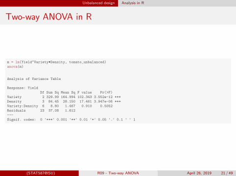
Two-way ANOVA in R
m = lm(Yield~Variety*Density, tomato_unbalanced)
anova(m)
Analysis of Variance Table
Response: Yield
Df Sum Sq Mean Sq F value Pr(>F)
Variety 2 329.99 164.994 102.343 3.552e-12 ***
Density 3 84.45 28.150 17.461 3.947e-06 ***
Variety:Density 6 8.80 1.467 0.910 0.5052
Residuals 23 37.08 1.612
---
Signif. codes: 0 '***' 0.001 '**' 0.01 '*' 0.05 '.' 0.1 ' ' 1
(STAT587@ISU) R09 - Two-way ANOVA April 26, 2019 21 / 49

Unbalanced design Analysis in R
Variety comparison
emmeans(m, pairwise~Variety)
$emmeans
Variety emmean SE df lower.CL upper.CL
C 18.1 0.367 23 17.4 18.9
A 11.3 0.367 23 10.6 12.1
B 12.3 0.389 23 11.5 13.1
Results are averaged over the levels of: Density
Confidence level used: 0.95
$contrasts
contrast estimate SE df t.ratio p.value
C - A 6.792 0.518 23 13.102 <.0001
C - B 5.817 0.534 23 10.886 <.0001
A - B -0.975 0.534 23 -1.825 0.1839
Results are averaged over the levels of: Density
P value adjustment: tukey method for comparing a family of 3 estimates
(STAT587@ISU) R09 - Two-way ANOVA April 26, 2019 22 / 49

Unbalanced design Analysis in R
Density comparison
emmeans(m, pairwise~Density)
$emmeans
Density emmean SE df lower.CL upper.CL
10 11.5 0.423 23 10.6 12.4
20 14.4 0.423 23 13.5 15.3
30 15.9 0.457 23 15.0 16.9
40 13.9 0.423 23 13.0 14.8
Results are averaged over the levels of: Variety
Confidence level used: 0.95
$contrasts
contrast estimate SE df t.ratio p.value
10 - 20 -2.911 0.599 23 -4.864 0.0004
10 - 30 -4.433 0.623 23 -7.116 <.0001
10 - 40 -2.433 0.599 23 -4.065 0.0025
20 - 30 -1.522 0.623 23 -2.443 0.0967
20 - 40 0.478 0.599 23 0.798 0.8545
30 - 40 2.000 0.623 23 3.210 0.0189
Results are averaged over the levels of: Variety
P value adjustment: tukey method for comparing a family of 4 estimates
(STAT587@ISU) R09 - Two-way ANOVA April 26, 2019 23 / 49
Unbalanced design Analysis in R
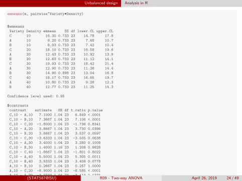
emmeans(m, pairwise~Variety*Density)
$emmeans
Variety Density emmean SE df lower.CL upper.CL
C 10 16.30 0.733 23 14.78 17.8
A 10 9.20 0.733 23 7.68 10.7
B 10 8.93 0.733 23 7.42 10.4
C 20 18.10 0.733 23 16.58 19.6
A 20 12.43 0.733 23 10.92 13.9
B 20 12.63 0.733 23 11.12 14.1
C 30 19.93 0.733 23 18.42 21.4
A 30 12.90 0.733 23 11.38 14.4
B 30 14.90 0.898 23 13.04 16.8
C 40 18.17 0.733 23 16.65 19.7
A 40 10.80 0.733 23 9.28 12.3
B 40 12.77 0.733 23 11.25 14.3
Confidence level used: 0.95
$contrasts
contrast estimate SE df t.ratio p.value
C,10 - A,10 7.1000 1.04 23 6.849 <.0001
C,10 - B,10 7.3667 1.04 23 7.106 <.0001
C,10 - C,20 -1.8000 1.04 23 -1.736 0.8341
C,10 - A,20 3.8667 1.04 23 3.730 0.0396
C,10 - B,20 3.6667 1.04 23 3.537 0.0597
C,10 - C,30 -3.6333 1.04 23 -3.505 0.0638
C,10 - A,30 3.4000 1.04 23 3.280 0.1008
C,10 - B,30 1.4000 1.16 23 1.208 0.9828
C,10 - C,40 -1.8667 1.04 23 -1.801 0.8022
C,10 - A,40 5.5000 1.04 23 5.305 0.0011
C,10 - B,40 3.5333 1.04 23 3.408 0.0778
A,10 - B,10 0.2667 1.04 23 0.257 1.0000
A,10 - C,20 -8.9000 1.04 23 -8.585 <.0001
A,10 - A,20 -3.2333 1.04 23 -3.119 0.1375
A,10 - B,20 -3.4333 1.04 23 -3.312 0.0945
A,10 - C,30 -10.7333 1.04 23 -10.353 <.0001
A,10 - A,30 -3.7000 1.04 23 -3.569 0.0558
A,10 - B,30 -5.7000 1.16 23 -4.918 0.0026
A,10 - C,40 -8.9667 1.04 23 -8.649 <.0001
A,10 - A,40 -1.6000 1.04 23 -1.543 0.9123
A,10 - B,40 -3.5667 1.04 23 -3.440 0.0729
B,10 - C,20 -9.1667 1.04 23 -8.842 <.0001
B,10 - A,20 -3.5000 1.04 23 -3.376 0.0831
B,10 - B,20 -3.7000 1.04 23 -3.569 0.0558
B,10 - C,30 -11.0000 1.04 23 -10.610 <.0001
B,10 - A,30 -3.9667 1.04 23 -3.826 0.0321
B,10 - B,30 -5.9667 1.16 23 -5.148 0.0015
B,10 - C,40 -9.2333 1.04 23 -8.906 <.0001
B,10 - A,40 -1.8667 1.04 23 -1.801 0.8022
B,10 - B,40 -3.8333 1.04 23 -3.698 0.0424
C,20 - A,20 5.6667 1.04 23 5.466 0.0007
C,20 - B,20 5.4667 1.04 23 5.273 0.0011
C,20 - C,30 -1.8333 1.04 23 -1.768 0.8185
C,20 - A,30 5.2000 1.04 23 5.016 0.0021
C,20 - B,30 3.2000 1.16 23 2.761 0.2592
C,20 - C,40 -0.0667 1.04 23 -0.064 1.0000
C,20 - A,40 7.3000 1.04 23 7.041 <.0001
C,20 - B,40 5.3333 1.04 23 5.144 0.0015
A,20 - B,20 -0.2000 1.04 23 -0.193 1.0000
A,20 - C,30 -7.5000 1.04 23 -7.234 <.0001
A,20 - A,30 -0.4667 1.04 23 -0.450 1.0000
A,20 - B,30 -2.4667 1.16 23 -2.128 0.6100
A,20 - C,40 -5.7333 1.04 23 -5.530 0.0006
A,20 - A,40 1.6333 1.04 23 1.575 0.9012
A,20 - B,40 -0.3333 1.04 23 -0.322 1.0000
B,20 - C,30 -7.3000 1.04 23 -7.041 <.0001
B,20 - A,30 -0.2667 1.04 23 -0.257 1.0000
B,20 - B,30 -2.2667 1.16 23 -1.956 0.7158
B,20 - C,40 -5.5333 1.04 23 -5.337 0.0010
B,20 - A,40 1.8333 1.04 23 1.768 0.8185
B,20 - B,40 -0.1333 1.04 23 -0.129 1.0000
C,30 - A,30 7.0333 1.04 23 6.784 <.0001
C,30 - B,30 5.0333 1.16 23 4.343 0.0100
C,30 - C,40 1.7667 1.04 23 1.704 0.8490
C,30 - A,40 9.1333 1.04 23 8.810 <.0001
C,30 - B,40 7.1667 1.04 23 6.913 <.0001
A,30 - B,30 -2.0000 1.16 23 -1.725 0.8392
A,30 - C,40 -5.2667 1.04 23 -5.080 0.0018
A,30 - A,40 2.1000 1.04 23 2.026 0.6736
A,30 - B,40 0.1333 1.04 23 0.129 1.0000
B,30 - C,40 -3.2667 1.16 23 -2.818 0.2355
B,30 - A,40 4.1000 1.16 23 3.537 0.0596
B,30 - B,40 2.1333 1.16 23 1.841 0.7810
C,40 - A,40 7.3667 1.04 23 7.106 <.0001
C,40 - B,40 5.4000 1.04 23 5.209 0.0013
A,40 - B,40 -1.9667 1.04 23 -1.897 0.7498
P value adjustment: tukey method for comparing a family of 12 estimates
(STAT587@ISU) R09 - Two-way ANOVA April 26, 2019 24 / 49

Unbalanced design Summary
Summary
The analysis can be completed just like the balanced design usingemmeans to answer scientific questions of interest.
(STAT587@ISU) R09 - Two-way ANOVA April 26, 2019 25 / 49
Incomplete design
Incomplete design
Suppose none of the samples from variety B, density 30 were obtained.
Now the analysis becomes more complicated.
(STAT587@ISU) R09 - Two-way ANOVA April 26, 2019 26 / 49
Incomplete design
Incomplete design
Suppose none of the samples from variety B, density 30 were obtained.Now the analysis becomes more complicated.
(STAT587@ISU) R09 - Two-way ANOVA April 26, 2019 26 / 49

Incomplete design
tomato_incomplete = tomato %>%
filter(!(Variety == "B" & Density == 30)) %>%
mutate(VarietyDensity = paste0(Variety,Density))
ggplot(tomato_incomplete, aes(x=Density, y=Yield, color=Variety)) + geom_jitter(height=0, width=0.1) + theme_bw()
8
12
16
20
10 20 30 40
Density
Yie
ld
Variety
C
A
B
(STAT587@ISU) R09 - Two-way ANOVA April 26, 2019 27 / 49

Incomplete design
Summary statistics
sm_incomplete = tomato_incomplete %>%
group_by(Variety, Density) %>%
summarize(n = n(),
mean = mean(Yield),
sd = sd(Yield))
sm_incomplete
# A tibble: 11 x 5
# Groups: Variety [?]
Variety Density n mean sd
<fct> <fct> <int> <dbl> <dbl>
1 C 10 3 16.3 1.11
2 C 20 3 18.1 1.35
3 C 30 3 19.9 1.68
4 C 40 3 18.2 0.874
5 A 10 3 9.2 1.30
6 A 20 3 12.4 1.10
7 A 30 3 12.9 0.985
8 A 40 3 10.8 1.7
9 B 10 3 8.93 1.04
10 B 20 3 12.6 1.10
11 B 40 3 12.8 1.62
(STAT587@ISU) R09 - Two-way ANOVA April 26, 2019 28 / 49
Incomplete design Treat as a One-way ANOVA
Treat as a One-way ANOVA
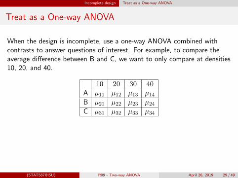
When the design is incomplete, use a one-way ANOVA combined withcontrasts to answer questions of interest.
For example, to compare theaverage difference between B and C, we want to only compare at densities10, 20, and 40.
10 20 30 40
A µ11 µ12 µ13 µ14B µ21 µ22 µ23 µ24C µ31 µ32 µ33 µ34
Thus, the contrast is
γ = 13(µ31 + µ32 + µ34)− 1
3(µ21 + µ22 + µ24)= 1
3(µ31 + µ32 + µ34 − µ21 − µ22 − µ24)
(STAT587@ISU) R09 - Two-way ANOVA April 26, 2019 29 / 49
Incomplete design Treat as a One-way ANOVA
Treat as a One-way ANOVA
When the design is incomplete, use a one-way ANOVA combined withcontrasts to answer questions of interest. For example, to compare theaverage difference between B and C, we want to only compare at densities10, 20, and 40.
10 20 30 40
A µ11 µ12 µ13 µ14B µ21 µ22 µ23 µ24C µ31 µ32 µ33 µ34
Thus, the contrast is
γ = 13(µ31 + µ32 + µ34)− 1
3(µ21 + µ22 + µ24)= 1
3(µ31 + µ32 + µ34 − µ21 − µ22 − µ24)
(STAT587@ISU) R09 - Two-way ANOVA April 26, 2019 29 / 49
Incomplete design Treat as a One-way ANOVA
The Regression model
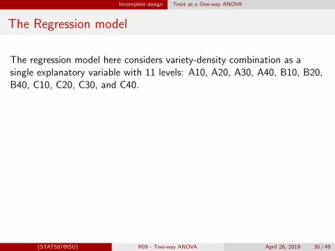
The regression model here considers variety-density combination as asingle explanatory variable with 11 levels: A10, A20, A30, A40, B10, B20,B40, C10, C20, C30, and C40.
Let C40 be the reference level. Forobservation i, let
Yi be the yield
Vi be the variety
Di be the density
The model is then Yiind∼ N(µi, σ
2) and
µi = β0+β1I(Vi = A,Di = 10)+β2I(Vi = A,Di = 20)+β3I(Vi = A,Di = 30) +β4I(Vi = A,Di = 40)+β5I(Vi = B,Di = 10)+β6I(Vi = B,Di = 20) +β7I(Vi = B,Di = 40)+β8I(Vi = C,Di = 10)+β9I(Vi = C,Di = 20)+β10I(Vi = C,Di = 30)
(STAT587@ISU) R09 - Two-way ANOVA April 26, 2019 30 / 49

Incomplete design Treat as a One-way ANOVA
The Regression model
The regression model here considers variety-density combination as asingle explanatory variable with 11 levels: A10, A20, A30, A40, B10, B20,B40, C10, C20, C30, and C40. Let C40 be the reference level.
Forobservation i, let
Yi be the yield
Vi be the variety
Di be the density
The model is then Yiind∼ N(µi, σ
2) and
µi = β0+β1I(Vi = A,Di = 10)+β2I(Vi = A,Di = 20)+β3I(Vi = A,Di = 30) +β4I(Vi = A,Di = 40)+β5I(Vi = B,Di = 10)+β6I(Vi = B,Di = 20) +β7I(Vi = B,Di = 40)+β8I(Vi = C,Di = 10)+β9I(Vi = C,Di = 20)+β10I(Vi = C,Di = 30)
(STAT587@ISU) R09 - Two-way ANOVA April 26, 2019 30 / 49

Incomplete design Treat as a One-way ANOVA
The Regression model
The regression model here considers variety-density combination as asingle explanatory variable with 11 levels: A10, A20, A30, A40, B10, B20,B40, C10, C20, C30, and C40. Let C40 be the reference level. Forobservation i, let
Yi be the yield
Vi be the variety
Di be the density
The model is then Yiind∼ N(µi, σ
2) and
µi = β0+β1I(Vi = A,Di = 10)+β2I(Vi = A,Di = 20)+β3I(Vi = A,Di = 30) +β4I(Vi = A,Di = 40)+β5I(Vi = B,Di = 10)+β6I(Vi = B,Di = 20) +β7I(Vi = B,Di = 40)+β8I(Vi = C,Di = 10)+β9I(Vi = C,Di = 20)+β10I(Vi = C,Di = 30)
(STAT587@ISU) R09 - Two-way ANOVA April 26, 2019 30 / 49

Incomplete design Analysis in R
Two-way ANOVA in R
m <- lm(Yield ~ Variety*Density, data=tomato_incomplete)
anova(m)
Analysis of Variance Table
Response: Yield
Df Sum Sq Mean Sq F value Pr(>F)
Variety 2 347.38 173.691 104.462 5.868e-12 ***
Density 3 66.65 22.218 13.362 3.514e-05 ***
Variety:Density 5 7.06 1.412 0.849 0.53
Residuals 22 36.58 1.663
---
Signif. codes: 0 '***' 0.001 '**' 0.01 '*' 0.05 '.' 0.1 ' ' 1
How can you tell the design is not complete?
(STAT587@ISU) R09 - Two-way ANOVA April 26, 2019 31 / 49

Incomplete design Analysis in R
One-way ANOVA in R
m = lm(Yield~Variety:Density, tomato_incomplete)
anova(m)
Analysis of Variance Table
Response: Yield
Df Sum Sq Mean Sq F value Pr(>F)
Variety:Density 10 421.09 42.109 25.326 8.563e-10 ***
Residuals 22 36.58 1.663
---
Signif. codes: 0 '***' 0.001 '**' 0.01 '*' 0.05 '.' 0.1 ' ' 1
(STAT587@ISU) R09 - Two-way ANOVA April 26, 2019 32 / 49

Incomplete design Analysis in R
Contrasts
# Note the -1 in order to construct the contrast
m = lm(Yield ~ VarietyDensity, tomato_incomplete)
em <- emmeans(m, ~ VarietyDensity)
contrast(em, method = list(
# A10 A20 A30 A40 B10 B20 B40 C10 C20 C30 C40
"C-B" = c( 0, 0, 0, 0, -1, -1, -1, 1, 1, 0, 1)/3,
"C-A" = c( -1, -1, -1, -1, 0, 0, 0, 1, 1, 1, 1)/4,
"B-A" = c( -1, -1, 0, -1, 1, 1, 1, 0, 0, 0, 0)/3)) %>%
confint
contrast estimate SE df lower.CL upper.CL
C-B 6.078 0.608 22 4.817 7.34
C-A 6.792 0.526 22 5.700 7.88
B-A 0.633 0.608 22 -0.627 1.89
Confidence level used: 0.95
(STAT587@ISU) R09 - Two-way ANOVA April 26, 2019 33 / 49

Incomplete design Analysis in R
m = lm(Yield~Variety:Density, tomato_incomplete)
emmeans(m, pairwise~Variety:Density)
$emmeans
Variety Density emmean SE df lower.CL upper.CL
C 10 16.30 0.744 22 14.76 17.8
A 10 9.20 0.744 22 7.66 10.7
B 10 8.93 0.744 22 7.39 10.5
C 20 18.10 0.744 22 16.56 19.6
A 20 12.43 0.744 22 10.89 14.0
B 20 12.63 0.744 22 11.09 14.2
C 30 19.93 0.744 22 18.39 21.5
A 30 12.90 0.744 22 11.36 14.4
B 30 nonEst NA NA NA NA
C 40 18.17 0.744 22 16.62 19.7
A 40 10.80 0.744 22 9.26 12.3
B 40 12.77 0.744 22 11.22 14.3
Confidence level used: 0.95
$contrasts
contrast estimate SE df t.ratio p.value
C,10 - A,10 7.1000 1.05 22 6.744 <.0001
C,10 - B,10 7.3667 1.05 22 6.997 <.0001
C,10 - C,20 -1.8000 1.05 22 -1.710 0.8458
C,10 - A,20 3.8667 1.05 22 3.673 0.0465
C,10 - B,20 3.6667 1.05 22 3.483 0.0688
C,10 - C,30 -3.6333 1.05 22 -3.451 0.0734
C,10 - A,30 3.4000 1.05 22 3.229 0.1136
C,10 - B,30 nonEst NA NA NA NA
C,10 - C,40 -1.8667 1.05 22 -1.773 0.8156
C,10 - A,40 5.5000 1.05 22 5.224 0.0014
C,10 - B,40 3.5333 1.05 22 3.356 0.0887
A,10 - B,10 0.2667 1.05 22 0.253 1.0000
A,10 - C,20 -8.9000 1.05 22 -8.453 <.0001
A,10 - A,20 -3.2333 1.05 22 -3.071 0.1529
A,10 - B,20 -3.4333 1.05 22 -3.261 0.1069
A,10 - C,30 -10.7333 1.05 22 -10.195 <.0001
A,10 - A,30 -3.7000 1.05 22 -3.514 0.0645
A,10 - B,30 nonEst NA NA NA NA
A,10 - C,40 -8.9667 1.05 22 -8.517 <.0001
A,10 - A,40 -1.6000 1.05 22 -1.520 0.9193
A,10 - B,40 -3.5667 1.05 22 -3.388 0.0833
B,10 - C,20 -9.1667 1.05 22 -8.707 <.0001
B,10 - A,20 -3.5000 1.05 22 -3.324 0.0945
B,10 - B,20 -3.7000 1.05 22 -3.514 0.0645
B,10 - C,30 -11.0000 1.05 22 -10.448 <.0001
B,10 - A,30 -3.9667 1.05 22 -3.768 0.0380
B,10 - B,30 nonEst NA NA NA NA
B,10 - C,40 -9.2333 1.05 22 -8.770 <.0001
B,10 - A,40 -1.8667 1.05 22 -1.773 0.8156
B,10 - B,40 -3.8333 1.05 22 -3.641 0.0497
C,20 - A,20 5.6667 1.05 22 5.382 0.0010
C,20 - B,20 5.4667 1.05 22 5.192 0.0015
C,20 - C,30 -1.8333 1.05 22 -1.741 0.8310
C,20 - A,30 5.2000 1.05 22 4.939 0.0028
C,20 - B,30 nonEst NA NA NA NA
C,20 - C,40 -0.0667 1.05 22 -0.063 1.0000
C,20 - A,40 7.3000 1.05 22 6.934 <.0001
C,20 - B,40 5.3333 1.05 22 5.066 0.0021
A,20 - B,20 -0.2000 1.05 22 -0.190 1.0000
A,20 - C,30 -7.5000 1.05 22 -7.124 <.0001
A,20 - A,30 -0.4667 1.05 22 -0.443 1.0000
A,20 - B,30 nonEst NA NA NA NA
A,20 - C,40 -5.7333 1.05 22 -5.446 0.0009
A,20 - A,40 1.6333 1.05 22 1.551 0.9090
A,20 - B,40 -0.3333 1.05 22 -0.317 1.0000
B,20 - C,30 -7.3000 1.05 22 -6.934 <.0001
B,20 - A,30 -0.2667 1.05 22 -0.253 1.0000
B,20 - B,30 nonEst NA NA NA NA
B,20 - C,40 -5.5333 1.05 22 -5.256 0.0013
B,20 - A,40 1.8333 1.05 22 1.741 0.8310
B,20 - B,40 -0.1333 1.05 22 -0.127 1.0000
C,30 - A,30 7.0333 1.05 22 6.680 0.0001
C,30 - B,30 nonEst NA NA NA NA
C,30 - C,40 1.7667 1.05 22 1.678 0.8599
C,30 - A,40 9.1333 1.05 22 8.675 <.0001
C,30 - B,40 7.1667 1.05 22 6.807 <.0001
A,30 - B,30 nonEst NA NA NA NA
A,30 - C,40 -5.2667 1.05 22 -5.002 0.0024
A,30 - A,40 2.1000 1.05 22 1.995 0.6923
A,30 - B,40 0.1333 1.05 22 0.127 1.0000
B,30 - C,40 nonEst NA NA NA NA
B,30 - A,40 nonEst NA NA NA NA
B,30 - B,40 nonEst NA NA NA NA
C,40 - A,40 7.3667 1.05 22 6.997 <.0001
C,40 - B,40 5.4000 1.05 22 5.129 0.0018
A,40 - B,40 -1.9667 1.05 22 -1.868 0.7656
P value adjustment: tukey method for comparing a family of 12 estimates
# We could have used the VarietyDensity model, but this looks nicer
(STAT587@ISU) R09 - Two-way ANOVA April 26, 2019 34 / 49

Incomplete design Summary
Summary
When dealing with an incomplete design, it is often easier to treat theanalysis as a one-way ANOVA and use contrasts to answer scientificquestions of interest.
(STAT587@ISU) R09 - Two-way ANOVA April 26, 2019 35 / 49

Optimal yield
Optimal yield
Now suppose you have the same data set, but your scientific question isdifferent.
Specifically, you are interested in choosing a variety-densitycombination that provides the optimal yield.
You can use the ANOVA analysis to choose from amongst the 3 varietiesand one of the 4 densities, but there is no reason to believe that theoptimal density will be one of those 4.
(STAT587@ISU) R09 - Two-way ANOVA April 26, 2019 36 / 49
Optimal yield
Optimal yield
Now suppose you have the same data set, but your scientific question isdifferent. Specifically, you are interested in choosing a variety-densitycombination that provides the optimal yield.
You can use the ANOVA analysis to choose from amongst the 3 varietiesand one of the 4 densities, but there is no reason to believe that theoptimal density will be one of those 4.
(STAT587@ISU) R09 - Two-way ANOVA April 26, 2019 36 / 49

Optimal yield
Optimal yield
Now suppose you have the same data set, but your scientific question isdifferent. Specifically, you are interested in choosing a variety-densitycombination that provides the optimal yield.
You can use the ANOVA analysis to choose from amongst the 3 varietiesand one of the 4 densities
, but there is no reason to believe that theoptimal density will be one of those 4.
(STAT587@ISU) R09 - Two-way ANOVA April 26, 2019 36 / 49

Optimal yield
Optimal yield
Now suppose you have the same data set, but your scientific question isdifferent. Specifically, you are interested in choosing a variety-densitycombination that provides the optimal yield.
You can use the ANOVA analysis to choose from amongst the 3 varietiesand one of the 4 densities, but there is no reason to believe that theoptimal density will be one of those 4.
(STAT587@ISU) R09 - Two-way ANOVA April 26, 2019 36 / 49

Optimal yield
8
12
16
20
10 20 30 40
Density
Yie
ld
Variety
C
A
B
(STAT587@ISU) R09 - Two-way ANOVA April 26, 2019 37 / 49
Optimal yield Modeling
Modeling
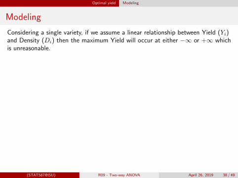
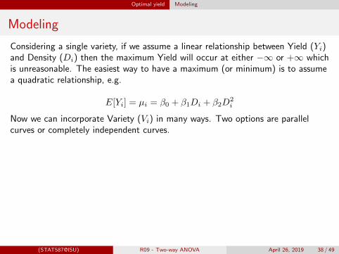
Considering a single variety, if we assume a linear relationship between Yield (Yi)and Density (Di) then the maximum Yield will occur at either −∞ or +∞ whichis unreasonable.
The easiest way to have a maximum (or minimum) is to assumea quadratic relationship, e.g.
E[Yi] = µi = β0 + β1Di + β2D2i
Now we can incorporate Variety (Vi) in many ways. Two options are parallelcurves or completely independent curves.
Parallel curves:
µi = β0 + β1Di + β2D2i
+β3I(Vi = A) + β4I(Vi = B)
Independent curves:
µi = β0 + β1Di + β2D2i
+β3I(Vi = A) + β4I(Vi = B)+β5I(Vi = A)Di + β6I(Vi = B)Di
+β7I(Vi = A)D2i + β8I(Vi = B)D2
i
(STAT587@ISU) R09 - Two-way ANOVA April 26, 2019 38 / 49

Optimal yield Modeling
Modeling
Considering a single variety, if we assume a linear relationship between Yield (Yi)and Density (Di) then the maximum Yield will occur at either −∞ or +∞ whichis unreasonable. The easiest way to have a maximum (or minimum) is to assumea quadratic relationship, e.g.
E[Yi] = µi = β0 + β1Di + β2D2i
Now we can incorporate Variety (Vi) in many ways.
Two options are parallelcurves or completely independent curves.
Parallel curves:
µi = β0 + β1Di + β2D2i
+β3I(Vi = A) + β4I(Vi = B)
Independent curves:
µi = β0 + β1Di + β2D2i
+β3I(Vi = A) + β4I(Vi = B)+β5I(Vi = A)Di + β6I(Vi = B)Di
+β7I(Vi = A)D2i + β8I(Vi = B)D2
i
(STAT587@ISU) R09 - Two-way ANOVA April 26, 2019 38 / 49
Optimal yield Modeling
Modeling
Considering a single variety, if we assume a linear relationship between Yield (Yi)and Density (Di) then the maximum Yield will occur at either −∞ or +∞ whichis unreasonable. The easiest way to have a maximum (or minimum) is to assumea quadratic relationship, e.g.
E[Yi] = µi = β0 + β1Di + β2D2i
Now we can incorporate Variety (Vi) in many ways. Two options are parallelcurves or completely independent curves.
Parallel curves:
µi = β0 + β1Di + β2D2i
+β3I(Vi = A) + β4I(Vi = B)
Independent curves:
µi = β0 + β1Di + β2D2i
+β3I(Vi = A) + β4I(Vi = B)+β5I(Vi = A)Di + β6I(Vi = B)Di
+β7I(Vi = A)D2i + β8I(Vi = B)D2
i
(STAT587@ISU) R09 - Two-way ANOVA April 26, 2019 38 / 49

Optimal yield Modeling
Modeling
Considering a single variety, if we assume a linear relationship between Yield (Yi)and Density (Di) then the maximum Yield will occur at either −∞ or +∞ whichis unreasonable. The easiest way to have a maximum (or minimum) is to assumea quadratic relationship, e.g.
E[Yi] = µi = β0 + β1Di + β2D2i
Now we can incorporate Variety (Vi) in many ways. Two options are parallelcurves or completely independent curves.
Parallel curves:
µi = β0 + β1Di + β2D2i
+β3I(Vi = A) + β4I(Vi = B)
Independent curves:
µi = β0 + β1Di + β2D2i
+β3I(Vi = A) + β4I(Vi = B)+β5I(Vi = A)Di + β6I(Vi = B)Di
+β7I(Vi = A)D2i + β8I(Vi = B)D2
i
(STAT587@ISU) R09 - Two-way ANOVA April 26, 2019 38 / 49

Optimal yield Modeling
8
12
16
20
10 20 30 40
Density
Yie
ld
No variety
8
12
16
20
10 20 30 40
Density
Yie
ld
Variety
C
A
B
Parallel curves
8
12
16
20
10 20 30 40
Density
Yie
ld
Variety
C
A
B
Independent curves
(STAT587@ISU) R09 - Two-way ANOVA April 26, 2019 39 / 49
Optimal yield Modeling
Finding the maximum
For a particular variety, there will be an equation like
E[Yi] = µi = β0 + β1Di + β2D2i
where these β1 and β2 need not correspond to any particular β1 and β2 wehave discussed thus far.
If β2 < 0, then the quadratic curve has a maximum and it occurs at−β1/2β2.
(STAT587@ISU) R09 - Two-way ANOVA April 26, 2019 40 / 49
Optimal yield Analysis in R
No variety
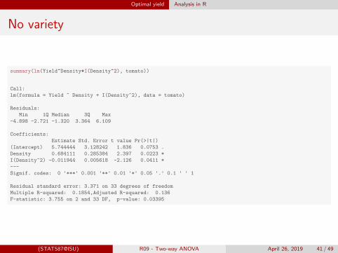
summary(lm(Yield~Density+I(Density^2), tomato))
Call:
lm(formula = Yield ~ Density + I(Density^2), data = tomato)
Residuals:
Min 1Q Median 3Q Max
-4.898 -2.721 -1.320 3.364 6.109
Coefficients:
Estimate Std. Error t value Pr(>|t|)
(Intercept) 5.744444 3.128242 1.836 0.0753 .
Density 0.684111 0.285384 2.397 0.0223 *
I(Density^2) -0.011944 0.005618 -2.126 0.0411 *
---
Signif. codes: 0 '***' 0.001 '**' 0.01 '*' 0.05 '.' 0.1 ' ' 1
Residual standard error: 3.371 on 33 degrees of freedom
Multiple R-squared: 0.1854,Adjusted R-squared: 0.136
F-statistic: 3.755 on 2 and 33 DF, p-value: 0.03395
(STAT587@ISU) R09 - Two-way ANOVA April 26, 2019 41 / 49

Optimal yield Analysis in R
Parallel curves
summary(lm(Yield~Density+I(Density^2) + Variety, tomato))
Call:
lm(formula = Yield ~ Density + I(Density^2) + Variety, data = tomato)
Residuals:
Min 1Q Median 3Q Max
-2.3422 -0.9039 0.1744 0.8082 2.1828
Coefficients:
Estimate Std. Error t value Pr(>|t|)
(Intercept) 9.980556 1.184193 8.428 1.61e-09 ***
Density 0.684111 0.104707 6.534 2.71e-07 ***
I(Density^2) -0.011944 0.002061 -5.794 2.21e-06 ***
VarietyA -6.791667 0.504942 -13.450 1.76e-14 ***
VarietyB -5.916667 0.504942 -11.718 6.39e-13 ***
---
Signif. codes: 0 '***' 0.001 '**' 0.01 '*' 0.05 '.' 0.1 ' ' 1
Residual standard error: 1.237 on 31 degrees of freedom
Multiple R-squared: 0.897,Adjusted R-squared: 0.8837
F-statistic: 67.48 on 4 and 31 DF, p-value: 7.469e-15
(STAT587@ISU) R09 - Two-way ANOVA April 26, 2019 42 / 49

Optimal yield Analysis in R
Independent curves
summary(lm(Yield~Density*Variety+I(Density^2)*Variety, tomato))
Call:
lm(formula = Yield ~ Density * Variety + I(Density^2) * Variety,
data = tomato)
Residuals:
Min 1Q Median 3Q Max
-2.04500 -0.82125 -0.01417 0.94000 1.71000
Coefficients:
Estimate Std. Error t value Pr(>|t|)
(Intercept) 11.808333 1.968364 5.999 2.12e-06 ***
Density 0.520167 0.179570 2.897 0.00739 **
VarietyA -8.458333 2.783687 -3.039 0.00523 **
VarietyB -9.733333 2.783687 -3.497 0.00165 **
I(Density^2) -0.008917 0.003535 -2.522 0.01787 *
Density:VarietyA 0.199167 0.253951 0.784 0.43971
Density:VarietyB 0.292667 0.253951 1.152 0.25924
VarietyA:I(Density^2) -0.004417 0.005000 -0.883 0.38482
VarietyB:I(Density^2) -0.004667 0.005000 -0.933 0.35889
---
Signif. codes: 0 '***' 0.001 '**' 0.01 '*' 0.05 '.' 0.1 ' ' 1
Residual standard error: 1.225 on 27 degrees of freedom
Multiple R-squared: 0.912,Adjusted R-squared: 0.886
F-statistic: 34.99 on 8 and 27 DF, p-value: 2.678e-12
(STAT587@ISU) R09 - Two-way ANOVA April 26, 2019 43 / 49

Randomized complete block design
Completely randomized design (CRD)
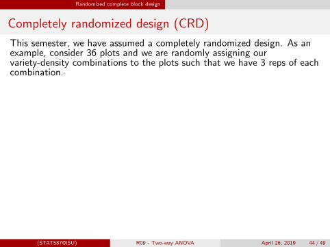
This semester, we have assumed a completely randomized design.
As anexample, consider 36 plots and we are randomly assigning ourvariety-density combinations to the plots such that we have 3 reps of eachcombination. The result may look something like this
C20
A10
C10
B40
C20
A20
B30
C40
B20
C30
C40
A30
B20
A10
B20
B40
C40
A40
B30
B10
A30
C10
B30
C20
C30
A30
B10
A20
A10
A40
C30
B10
A20
C10
A40
B40
(STAT587@ISU) R09 - Two-way ANOVA April 26, 2019 44 / 49
Randomized complete block design
Completely randomized design (CRD)
This semester, we have assumed a completely randomized design. As anexample, consider 36 plots and we are randomly assigning ourvariety-density combinations to the plots such that we have 3 reps of eachcombination.
The result may look something like this
C20
A10
C10
B40
C20
A20
B30
C40
B20
C30
C40
A30
B20
A10
B20
B40
C40
A40
B30
B10
A30
C10
B30
C20
C30
A30
B10
A20
A10
A40
C30
B10
A20
C10
A40
B40
(STAT587@ISU) R09 - Two-way ANOVA April 26, 2019 44 / 49

Randomized complete block design
Completely randomized design (CRD)
This semester, we have assumed a completely randomized design. As anexample, consider 36 plots and we are randomly assigning ourvariety-density combinations to the plots such that we have 3 reps of eachcombination. The result may look something like this
C20
A10
C10
B40
C20
A20
B30
C40
B20
C30
C40
A30
B20
A10
B20
B40
C40
A40
B30
B10
A30
C10
B30
C20
C30
A30
B10
A20
A10
A40
C30
B10
A20
C10
A40
B40
(STAT587@ISU) R09 - Two-way ANOVA April 26, 2019 44 / 49

Randomized complete block design
Complete randomized block design (RBD)
A randomized block design is appropriate when there is a nuisance factorthat you want to control for.
In our example, imagine you had 12 plots at3 different locations and you expect these locations would have impact onyield. A randomized block design might look like this.
C40
A10
B20
C20
C10
A30
A40
A20
B30
C30
B10
B40
C20
B30
A30
C40
C10
A20
B10
A40
A10
C30
B20
B40
B20
A30
C40
A40
C20
A10
C30
B10
A20
C10
B30
B40
Block 1 Block 2 Block 3
(STAT587@ISU) R09 - Two-way ANOVA April 26, 2019 45 / 49
Randomized complete block design
Complete randomized block design (RBD)
A randomized block design is appropriate when there is a nuisance factorthat you want to control for. In our example, imagine you had 12 plots at3 different locations and you expect these locations would have impact onyield.
A randomized block design might look like this.
C40
A10
B20
C20
C10
A30
A40
A20
B30
C30
B10
B40
C20
B30
A30
C40
C10
A20
B10
A40
A10
C30
B20
B40
B20
A30
C40
A40
C20
A10
C30
B10
A20
C10
B30
B40
Block 1 Block 2 Block 3
(STAT587@ISU) R09 - Two-way ANOVA April 26, 2019 45 / 49

Randomized complete block design
Complete randomized block design (RBD)
A randomized block design is appropriate when there is a nuisance factorthat you want to control for. In our example, imagine you had 12 plots at3 different locations and you expect these locations would have impact onyield. A randomized block design might look like this.
C40
A10
B20
C20
C10
A30
A40
A20
B30
C30
B10
B40
C20
B30
A30
C40
C10
A20
B10
A40
A10
C30
B20
B40
B20
A30
C40
A40
C20
A10
C30
B10
A20
C10
B30
B40
Block 1 Block 2 Block 3
(STAT587@ISU) R09 - Two-way ANOVA April 26, 2019 45 / 49

Randomized complete block design RBD Analysis
RBD Analysis
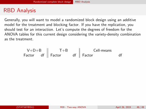
Generally, you will want to model a randomized block design using an additivemodel for the treatment and blocking factor.
If you have the replication, youshould test for an interaction. Let’s compute the degrees of freedom for theANOVA tables for this current design considering the variety-density combinationas the treatment.
V+D+B T+B Cell-meansFactor df Factor df Factor dfVariety 2Density 3 Treatment 11 Treatment 11Block 2 Block 2 Block 2
Treatment x Block 22Error 28 Error 22 Error 0Total 35 Total 35 Total 35
The cell-means model does not have enough degrees of freedom to estimate the
interacion because there is no replication of the treatment within a block.
(STAT587@ISU) R09 - Two-way ANOVA April 26, 2019 46 / 49

Randomized complete block design RBD Analysis
RBD Analysis
Generally, you will want to model a randomized block design using an additivemodel for the treatment and blocking factor. If you have the replication, youshould test for an interaction.
Let’s compute the degrees of freedom for theANOVA tables for this current design considering the variety-density combinationas the treatment.
V+D+B T+B Cell-meansFactor df Factor df Factor dfVariety 2Density 3 Treatment 11 Treatment 11Block 2 Block 2 Block 2
Treatment x Block 22Error 28 Error 22 Error 0Total 35 Total 35 Total 35
The cell-means model does not have enough degrees of freedom to estimate the
interacion because there is no replication of the treatment within a block.
(STAT587@ISU) R09 - Two-way ANOVA April 26, 2019 46 / 49
Randomized complete block design RBD Analysis
RBD Analysis
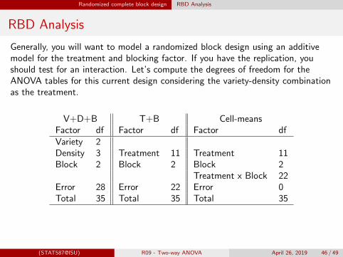
Generally, you will want to model a randomized block design using an additivemodel for the treatment and blocking factor. If you have the replication, youshould test for an interaction. Let’s compute the degrees of freedom for theANOVA tables for this current design considering the variety-density combinationas the treatment.
V+D+B T+B Cell-meansFactor df Factor df Factor dfVariety 2Density 3 Treatment 11 Treatment 11Block 2 Block 2 Block 2
Treatment x Block 22Error 28 Error 22 Error 0Total 35 Total 35 Total 35
The cell-means model does not have enough degrees of freedom to estimate the
interacion because there is no replication of the treatment within a block.
(STAT587@ISU) R09 - Two-way ANOVA April 26, 2019 46 / 49
Randomized complete block design RBD Analysis
RBD Analysis
Generally, you will want to model a randomized block design using an additivemodel for the treatment and blocking factor. If you have the replication, youshould test for an interaction. Let’s compute the degrees of freedom for theANOVA tables for this current design considering the variety-density combinationas the treatment.
V+D+B T+B Cell-meansFactor df Factor df Factor df
Variety 2Density 3 Treatment 11 Treatment 11Block 2 Block 2 Block 2
Treatment x Block 22Error 28 Error 22 Error 0Total 35 Total 35 Total 35
The cell-means model does not have enough degrees of freedom to estimate the
interacion because there is no replication of the treatment within a block.
(STAT587@ISU) R09 - Two-way ANOVA April 26, 2019 46 / 49
Randomized complete block design RBD Analysis
RBD Analysis
Generally, you will want to model a randomized block design using an additivemodel for the treatment and blocking factor. If you have the replication, youshould test for an interaction. Let’s compute the degrees of freedom for theANOVA tables for this current design considering the variety-density combinationas the treatment.
V+D+B T+B Cell-meansFactor df Factor df Factor dfVariety 2Density 3 Treatment 11 Treatment 11Block 2 Block 2 Block 2
Treatment x Block 22Error 28 Error 22 Error 0Total 35 Total 35 Total 35
The cell-means model does not have enough degrees of freedom to estimate the
interacion because there is no replication of the treatment within a block.
(STAT587@ISU) R09 - Two-way ANOVA April 26, 2019 46 / 49

Randomized complete block design RBD Analysis
RBD Analysis
Generally, you will want to model a randomized block design using an additivemodel for the treatment and blocking factor. If you have the replication, youshould test for an interaction. Let’s compute the degrees of freedom for theANOVA tables for this current design considering the variety-density combinationas the treatment.
V+D+B T+B Cell-meansFactor df Factor df Factor dfVariety 2Density 3 Treatment 11 Treatment 11Block 2 Block 2 Block 2
Treatment x Block 22Error 28 Error 22 Error 0Total 35 Total 35 Total 35
The cell-means model does not have enough degrees of freedom to estimate the
interacion because there is no replication of the treatment within a block.(STAT587@ISU) R09 - Two-way ANOVA April 26, 2019 46 / 49
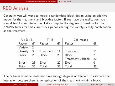

Randomized complete block design RBD Analysis
Why block?
Consider a simple experiment with 2 blocks each with 3 experimental unitsand 3 treatments (A, B, C).
C
A
B
A
B
C
B
A
B
A
C
C
Block 1 Block 2 Block 1 Block 2
Blocked Unblocked
Let’s consider 3 possible analyses:
Blocked experiment using an additive model for treatment and block(RBD)
Unblocked experiment using only treatment (CRD)
Unblocked experiment using an additive model for treatment andblock
(STAT587@ISU) R09 - Two-way ANOVA April 26, 2019 47 / 49
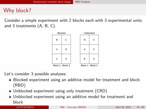

Randomized complete block design RBD Analysis
Why block?
Now suppose, the true model is
µij = µ+ Ti +Bj
where T1 = T2 = T3 and B1 = 0 and B2 = δ.
In the Blocked experiment using an additive model for treatment andblock, the expected treatment differences to all be zero.
In the Unblocked design using only treatment, the expected differencebetween treatments is
µC − µB = δ and µC − µA = δ/2.
In the Unblocked design using an additive model for treatment and block,we would have an unbalanced design and it would be impossible tocompare B and C.
(STAT587@ISU) R09 - Two-way ANOVA April 26, 2019 48 / 49
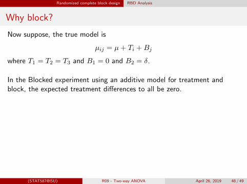

Randomized complete block design Summary
Summary
Block what you can control; randomize what you cannot.
(STAT587@ISU) R09 - Two-way ANOVA April 26, 2019 49 / 49