r - -uat - dtic.mil · Fault Tree Analysis-Basic Concepts ... in which it was stated that the...
216
_- _-uat r CmIi S ft II >5±4"''
Transcript of r - -uat - dtic.mil · Fault Tree Analysis-Basic Concepts ... in which it was stated that the...

_- _-uat r
CmIi
S ft
II
>5±4"''

NUREG-0492
Fault Tree Handbook
Date Published: January 1981
W. E. Vesely, U.S. Nuclear Regulatory CommissionF. F. Goldberg, U.S. Nuclear Regulatory Commission
N. H. Roberts, University of WashingtonD. F. Haasl, Institute of System Sciences, Inc.
Systems and Reliability ResearchOffice of Nuclear Regulatory ResearchU.S. Nuclear Regulatory CommissionWashington, D.C. 20555
RG &,, ý0
For sale by the U.S. Government Printing OfficeSuperintendent of Documents, Mail Stop: SSOP, Washington, DC 20402-9328
a, Q • /v2 -.2,-25-

Available from
GPO Sales ProgramDivision of Technical Information and Document Control
U.S. Nuclear Regulatory CommissionWashington, DC 20555
Printed copy price: $5.50
and
National Technical Information ServiceSpringfield, VA 22161

TABLE OF CONTENTS
Introduction . ............................................. vii
1. Basic Concepts of System Analysis .......................... l-1
1. The Purpose of System Analysis ........................ I-i2. Definition of a System . .............................. 1-33. Analytical Approaches .............................. 1-74. Perils and Pitfalls .................................. 1-9
II. Overview of Inductive Methods .............................. 1-1
1. Introduction ....................................... II-12. The "Parts Count" Approach ........................... 11-13. Failure Mode and Effect Analysis (FMEA) ................. II-24. Failure Mode Effect and Criticality Analysis (FMECA) ......... 11-45. Preliminary Hazard Analysis (PHA) ....................... 11-46. Fault Hazard Analysis (FHA) ........................... 11-57. Double Failure Matrix (DFM) ........................... 11-58. Success Path Models ................................. I-109. Conclusions ....................................... 11-12
III. Fault Tree Analysis-Basic Concepts .......................... 11n-1
1. Orientation ....................................... 111-12. Failure vs. Success Models ............................ 111-13. The Undesired Event Concept .......................... 111-34. Summary . ....................................... 111-4
IV. The Basic Elements of a Fault Tree .......................... IV-1
1. The Fault Tree Model ................................ IV-12. Symbology-The Building Blocks of the Fault Tree ............ IV-1
V. Fault Tree Construction Fundamentals ........................ V-1
1. Faults vs. Failures ................................... V-12. Fault Occurrence vs. Fault Existence ...................... V-13. Passive vs. Active Components ......................... V-24. Component Fault Categories: Primary, Secondary, and Command .. V-35. Failure Mechanism, Failure Mode, and Failure Effect .......... V-36. The "Immediate Cause" Concept ....................... V-67. Basic Rules for Fault Tree Construction .................... V-8
'i

iv TABLE OF CONTENTS
VI. Probability Theory-The Mathematical Description of Events ......... VI-I
1. Introduction VI-I2. Random Experiments and Outcomes of Random Experiments ..... VI-13. The Relative Frequency Definition of Probability ............. VI-34. Algebraic Operations with Probabilities ................... VI-35. Combinatorial Analysis .............................. VI-86. Set Theory: Application to the Mathematical Treatment
of Events ....................................... V I-I 17. Symbolism ........................................ VI-168. Additional Set Concepts ............................. VI-179. Bayes' Theorem ................................... VI-19
VII. Boolean Algebra and Application to Fault Tree Analysis ............ VII-1
1. Rules of Boolean Algebra ............................. VII-12. Application to Fault Tree Analysis ...................... VII-43. Shannon's Method for Expressing Boolean Functions in
Standardized Forms .................................. VII- 124. Determining the Minimal Cut Sets or Minimal Path Sets of a
Fault Tree ....................................... V II- 15
VIII. The Pressure Tank Example ............................... VIII-1
1. System Definition and Fault Tree Construction .............. VIII-12. Fault Tree Evaluation (Minimal Cut Sets) .................. VIII-12
IX. The Three Motor Example ................................ IX-1
1. System Definition and Fault Tree Construction .............. IX-12. Fault Tree Evaluation (Minimal Cut Sets) .................. IX-7
X. Probabilistic and Statistical Analyses ......................... X-1
1. Introduction ...................................... X-12. The Binomial Distribution ............................ X-13. The Cumulative Distribution Function ..................... X-74. The Probability Density Function ....................... X-95. Distribution Parameters and Moments .................... X-1O6. Limiting Forms of the Binomial: Normal, Poisson ............ X-157. Application of the Poisson Distribution to System Failures-
The So-Called Exponential Distribution ................... X-198. The Failure Rate Function ............................ X-229. An Application Involving the Time-to-Failure Distribution ....... X-25
10. Statistical Estimation . .............................. X-2611. Random Samples ................................... X-2712. Sampling Distributions . ............................. X-2713. Point Estimates-General ............................. X-28

TABLE OF CONTENTS
14. Point Estimates-Maximum Likelihood ................... X-3015. Interval Estimators .................................. X-3516. Bayesian Analyses ................................. X-39
XI. Fault Tree Evaluation Techniques ............................ XI-1
I. Introduction ..................................... XI-I2. Qualitative Evaluations .............................. XI-23. Quantitative Evaluations ............................. XI-7
XII. Fault Tree Evaluation Computer Codes ....................... XII-1
1. Overview of Available Codes ........................... XII-12. Computer Codes for Qualitative Analyses of Fault Trees ........ XII-23. Computer Codes for Quantitative Analyses of Fault Trees ....... XII-64. Direct Evaluation Codes ............................. XII-85. PL-MOD: A Dual Purpose Code ........................ XII-l 16. Common Cause Failure Analysis Codes .................... XII-12
Bibliography ............................................... BIB-l

INTRODUCTION
Since 1975, a short course entitled "System Safety and Reliability Analysis" hasbeen presented to over 200 NRC personnel and contractors. The course has beentaught jointly by David F. Haasl, Institute of System Sciences, Professor Norman H.Roberts, University of Washington, and 'members of the Probabilistic Analysis Staff,NRC, as part of a risk assessment training program sponsored by the ProbabilisticAnalysis Staff.
This handbook has been developed not only to serve as text for the System Safetyand Reliability Course, but also to make available to others a set of otherwiseundocumented material on fault tree construction and evaluation. The publication ofthis handbook is in accordance with the recommendations of the Risk AssessmentReview Group Report (NUREG/CR-04M0) in which it was stated that the fault/eventtree methodology both can and should be used more widely by the NRC. It is hopedthat this document will help to codify and systematize the fault tree approach tosystems analysis.
vii

CHAPTER I - BASIC CONCEPTS OF SYSTEM ANALYSIS
1. The Purpose of System Analysis
The principal concern of this book is the fault tree technique, which is asystematic method for acquiring information about a system.* The information sogained can be used in making decisions, and therefore, before we even define systemanalysis, we will undertake a brief examination of the decisionmaking process.Decisionmaking is a very complex process, and we will highlight only certain aspectswhich help to put a system analysis in proper context.
Presumably, any decision that we do make is based on our present knowledgeabout the situation at hand. This knowledge comes partly from our direct experiencewith the relevant situation or from related experience with similar situations. Ourknowledge may be increased by appropriate tests and proper analyses of theresults-that is, by experimentation. To some extent our knowledge may be based onconjecture ,nd this will be conditioned by our degree of optimism or pessimism. Forexample, we may be convinced that "all is for the best in this best of all possibleworlds." Or, conversely, we may believe in Murphy's Law: "If anything can gowrong, it will go wrong." Thus, knowledge may be obtained in several ways, but inthe vast majority of cases, it will not be possible to acquire all the relevantinformation, so that it is almost never possible to eliminate all elements ofuncertainty.
It is possible to postulate an imaginary world in which no decisions are made untilall the relevant information is assembled. This is a far cry from the everyday world inwhich decisions are forced on us by time, and not by the degree of completeness ofour knowledge. We all have deadlines to meet. Furthermore, because it is generallyimpossible to have all the relevant data at the time the decision must be made, wesimply cannot know all the consequences of electing to take a particular course ofaction. Figure 1-1 provides a schematic representation of these considerations.
INFORMATION
ACQUISITION
I INDRECT ,._. DECISION
INFORMATION IACQUISITION I
TIME AXIS
TIME AT WHICH 0/
DECISION MUST -J
BE MADE
Figure I-I. Schematic Representation of the Decisionmaking Process
*There are other methods for performing this function. Some of these are discussed brieflyin Chapter II.
I-1

1-2 FAULT TREE HANDBOOK
The existence of the time constraint on the decisionmaking process leads us tomake a distinction between good decisions and correct decisions. We can classify adecision as good or bad whenever we have the advantage of retrospect. I make adecision to buy 1000 shares of XYZ Corporation. Six months later, I find that thestock has risen 20 points. My original decision can now be classified as good. If,however, the stock has plummeted 20 points in the interim, I would have toconclude that my original decision was bad. Nevertheless, that original decision couldvery well have been correct if all the information available at the time had indicated arosy future for XYZ Corporation.
We are concerned here with making correct decisions. To do this we require:(1) The identification of that information (or those data) that would be pertinent
to the anticipated decision.(2) A systematic program for the acquisition of this pertinent information.(3) A rational assessment or analysis of the data so acquired.There are perhaps as many definitions of system analysis as there are people
working and writing in the field. The authors of this book, after long thought, somecontroversy, and considerable experience, have chosen the following definition:
System analysis is a directed process for the orderly and timely acquisition andinvestigation of specific system information pertinent to a given decision.
According to this definition, the primary function of the system analysis is theacquisition of information and not the generation of a system model. Our emphasis(at least initially) will be on the process (i.e., the acquisition of information) and noton the product (i.e., the system model). This emphasis is necessary because, in theabsence of a directed, manageable, and disciplined process, the corresponding systemmodel will not usually be a very fruitful one.
We must decide what information is relevant to a given decision before the datagathering activity starts. What information is essential? What information isdesirable? This may appear perfectly obvious, but it is astonishing on how manyoccasions this rationale is not followed. The sort of thing that may happen isillustrated in Figure 1-2.
Figure 1-2. Data Gathering Gone Awry

BASIC CONCEPTS OF SYSTEM ANALYSIS 1-3
The large circle represents the information that will be essential for a correct decisionto be made at some future time. Professor Jones, who is well funded and who is a"Very Senior Person," is an expert in sub-area A. He commences to investigate thisarea, and his investigation leads him to some fascinating unanswered questionsindicated in the sketch by A1 . Investigation of A1 leads to A2 , and so on. Notice,however, that Professor Jones' efforts are causing him to depart more and more fromthe area of essential data. Laboratory Alpha is in an excellent position to studysub-area B. These investigations lead to B1 and B2 and so on, and the same thing ishappening. When the time for decision arrives, all the essential information is notavailable despite the fact that the efforts expended would have been able to providethe necessary data if they had been properly directed.
The nature of the decisionmaking process is shown in Figure 1-3. Block Arepresents certified reality. Now actual reality is pretty much of a "closed book," butby experimentation and investigation (observations of Nature) we may slowlyconstruct a perception of reality. This is our system model shown as block B. Next,this model is analyzed to produce conclusions (block C) on which our decision willbe based. So our decision is a direct outcome of our model and if our model isgrossly in error, so also will be our decision. Clearly, then, in this process, the greatestemphasis should be placed on assuring that the system model provides as accurate arepresentation of reality as possible.
2 Z0 0
07- 7-
<t ,,T
REALITY OUR PERCEPTION BASIS FOROF REALITY DECISION
Figure 1-3. Relationship Between Reality, SystemModel, and Decision Process
2. Definition of a System
We have given a definition of the process of system analysis. Our next task is todevise a suitable definition for the word "system." In common parlance we speak of"the solar system," "a system of government," or a "communication system," and inso doing we imply some sort of organization existing among various elements that

1-4 FAULT TREE HANDBOOK
mutually interact in ways that may or may not be well defined. It seems reasonable,then, to establish the following definition:
A system is a deterministic entity comprising an interacting collection ofdiscrete elements.
From a practical standpoint, this is not very useful and, in particular cases, wemust specify what aspects of system performance are of immediate concern. Asystem performs certain functions and the selection of particular performanceaspects will dictate what kind of analysis is to be conducted. For instance: are weinterested in whether the system accomplishes some task successfully; are weinterested in whether the system fails in some hazardous way; or are we interested inwhether the system will prove more costly than originally anticipated? It could wellbe that the correct system analyses in these three cases will be based on differentsystem defintions.
The word "deterministic" in the definition implies that the system in question beidentifiable. It is completely futile to attempt an analysis of something that cannotbe clearly identified. The poet Dante treated the Inferno as a system and divided itup into a number of harrowing levels but, from a practical standpoint, such a systemis not susceptible to identification as would be, for example, the plumbing system inmy home. Furthermore, a system must have some purpose-it must do. something.Transportation systems, circulating hot water piping systems, local school systems allhave definite purposes and do not exist simply as figments of the imagination.
The discrete elements of the definition must also, of course, be identifiable; forinstance, the individual submarines in the Navy's Pacific Ocean Submarine Flotilla.Note that the discrete elements themselves may be regarded as systems. Thus, asubmarine consists of a propulsion system, a navigation system, a hull system, apiping system, and so forth; each of these, in turn, may be further broken down intosubsystems and sub-subsystems, etc.
Note also from the definition that a system is made up of parts.,br subsystems thatinteract. This interaction, which may be very complex indeed, generally insures thata system is not simply equal to the sum of its parts, a point that will be continuallyemphasized throughout this book. Furthermore, if the physical nature of any partchanges-for example by failure-the system itself also changes. This is an importantpoint because, should design changes be made as a result of a system analysis, thenew system so resulting will have to be subjected to an analysis of its own. Consider,for example, a four-engine aircraft. Suppose one engine fails. We now have a newsystem quite different from the original one. For one thing, the landing characteris-tics have changed rather drastically. Suppose two engines fail. We now have sixdifferent possible systems depending on which two engines are out of commission.
Perhaps the most vital decision that must be made in system definition is how toput external boundaries on the system. Consider the telephone sitting on the desk. Isit sufficient to define the system simply as the instrument itself (earpiece, cord andcradle), or should the line running to the jack in the wall be included? Should thejack itself be included? What about the external lines to the telephone pole? Whatabout the junction box on the pole? What about the vast complex of lines, switchingequipment, etc., that comprise the telephone system in the local area, the nation, the'

BASIC CONCEPTS OF SYSTEM ANALYSIS I-5
world? Clearly some external boundary to the system must be established and thisdecision will have to be made partially on the basis of what aspect of systemperformance is of concern. If the immediate problem is that the bell is not loudenough to attract my attention when I am in a remote part of the house, the externalsystem boundary will be fairly closed in. If the problem involves static on the line,the external boundary will be much further out.
It is also important in system definition to establish a limit of resolution. In thetelephone example, do I wish to extend my analysis to the individual components(screws, transmitter, etc.) of which the instrument is composed? Is it necessary todescend to the molecular level, the atomic level, the nuclear level? Here again, adecision can be made partially on the basis of the system aspect of interest.
What we have said so far can be represented as in Figure 1-4. The dotted lineseparates the system from the environment in which it is embedded. Thus, thisdotted line constitutes an external boundary. It is sometimes useful to divide thesystem into a number of subsystems, A, B, C, etc. There may be several motivationsfor doing this; most of them will be discussed in due course. Observe also that one ofthe subsystems, F, has been broken down, for purposes of the analysis, into itssmallest sub-subsystems. This constitutes a choice of an internal boundary for thesystem. The smallest sub-subsystems, a, b, c, etc., are the "discrete elements"mentioned in the general definition of a system.
TYPICALSUBSYSTEMS SYSTEM - ENVIRONMENT
IT BOUNDARY-- -..... .... XTRAA E
FI SMALLEST
I SUB-SUBSYSTEM
B a b c d e f p (LIMIT OF
g h i 1 k I A RESOLUTION)
m n p q r
Figure 1-4. System Definition: External and Internal Boundaries
The choice of the appropriate system boundaries in particular cases is a matter ofvital importance, for the choice of external boundaries determines the comprehen-siveness of the analysis, whereas the choice of a limit of resolution limits the detail ofthe analysis. A few further facets of this problem will be discussed briefly now, andwill be emphasized throughout the book, especially in the applications.
The system boundaries we have discussed so far have been physical boundaries. Itis also possible, and indeed necessary in many cases, to set up temporal or time-likeboundaries on a system. Consider a man who adopts the policy of habitually tradinghis present car in for a new one every two years. In this example, the system is the

1-6 FAULT TREE HANDBOOK
car and the system aspect of interest is the maintenance policy. It is clear that, underthe restriction of a two-year temporal boundary, the maintenance policy adoptedwill be one thing; it will be quite a different thing if the man intends to run the carfor as long as possible. In some applications, the system's physical boundaries mightactually be functions of time. An example of this would be a system whose temporalboundaries denote different operating phases or different design modifications. Aftereach phase change or design modification, the physical boundaries are subject toreview and possible alteration.
The system analyst must also ask the question, "Are the chosen systemboundaries feasible and are they valid in view of the goal of the analysis?" To reachcertain conclusions about a system, it may be desirable to include a large system"volume" within the external boundaries. This may call for an extensive,time-consuming analysis. If the money, time and staff available are inadequate forthis task and more efficient analysis approaches are not possible, then the externalboundaries must be "moved in" and the amount of information expected to resultfrom the analysis must be reduced. If I am concerned about my TV reception, itmight be desirable to include the state of the ionosphere in my analysis, but thiswould surely be infeasible. I would be better advised to reduce the goals of myanalysis to a determination of the optimum orientation of mv roof antenna.
The limit of resolution (internal boundary) can also be established fromconsiderations of feasibility (fortunately!) and from the goal of the analysis. It ispossible to conduct a worthwhile study of the reliability of a population of TV setswithout being concerned about what is going on at the microscopic andsubmicroscopic levels. If the system failure probability is to be calculated, then thelimit of resolution should cover component failures for which data are obtainable. Atany rate, once the limit of resolution has been chosen (and thus the "discreteelements" defined), it is interactions at this level with which we are concerned; weassume no knowledge and are not concerned about interactions taking place at lowerlevels.
We now see that the external boundaries serve to delineate system outputs (effectsof the system on its environment) and system inputs (effects of the environment onthe system); the limits of resolution serve to define the "discrete elements" of thesystem and to establish the basic interactions within the system.
The reader with a technical background will recognize that our definition of asystem and its boundaries is analogous to a similar process involved in classicalthermodynamics, in which an actual physical boundary or an imaginary one is usedto segregate a definite quantity of matter ("control mass") or a definite volume("control volume"). The inputs and outputs of the system are then identified by theamounts of energy or mass passing into or out of the bounded region. A system thatdoes not exchange mass with its environment is termed a "closed system" and aclosed system that does not exchange energy with its surroundings is termed an"adiabatic system" or an "isolated system." A student who has struggled withthermodynamic problems, particularly flow problems, will have been impressed withthe importance of establishing appropriate system boundaries before attempting asolution of the problem.
A good deal of thought must be expended in the proper assignment of systemboundaries and limits of resolution. Optimally speaking, the system boundaries and

BASIC CONCEPTS OF SYSTEM ANALYSIS 1-7
limits of resolution should be defined before the analysis begins and should beadhered to while the analysis is carried out. However, in practical situations theboundaries or limits of resolution may need to be changed because of informationgained during the analysis. For example, it may be found that system schematics arenot available in as detailed a form as originally conceived. The system boundaries andlimits of resolution, and any modifications, must be clearly defined in any analysis,and should be a chief section in any report that is issued.
0 04/ 10"4 •EXTENDED SYSTEM
/ •BOUNDARY/\S10-3 SYSTEM BOUNDARY
Figure 1-5. Effect of System Boundaries on Event Probabilities
To illustrate another facet of the bounding and resolution problem, considerFigure 1-5. The solid inner circle represents our system boundary inside of which weare considering events whose probabilities of occurrence are, say, of order 10-3 orgreater. If the system boundaries were extended (dotted circle) we would include, inaddition, events whose probabilities of occurrence were, say, of order 10-4 orgreater. By designing two-fold redundancy into our restricted system (solid circle) wecould reduce event probabilities there to the order of (10-3)(10-3) = 10-6 but thenthe probabilities of events that we are ignoring become overriding, and we aresuffering under the delusion that our system is two orders of magnitude safer ormore reliable than it actually is. When due consideration is not devoted to matterssuch as this, the naive reliability calculator will often produce such absurd numbersas 10-16 or 10-18. The low numbers simply say that the system is not going to failby the ways considered but instead is going to fail at a much higher probability in away not considered.
3. Analytical Approaches
Because we are concerned, in this volume, with certain formal processes ormodels, it should come as no great suprise that these processes or models can becategorized in exactly the same way as are the processes of thought employed in thehuman decisionmaking process. There are two generic analytical methods by meansof which conclusions are reached in the human sphere: induction and deduction. It isnecessary at this point to discuss the respective characteristics of these approaches.

1-8 FAULT TREE HANDBOOK
Inductive Approaches
Induction constitutes reasoning from individual cases to a general conclusion. If,in the consideration of a certain system, we postulate a particular fault or initiatingcondition and attempt to ascertain the effect of that fault or condition on systemoperation, we are constructing an inductive system analysis. Thus, we might inquireinto how the loss of some specified control surface affects the flight of an airplane orinto how the elimination of some item in the budget affects the overall operation ofa school district. We might also inquire how the non-insertion of given control rodsaffects a scram system's performance or how a given initiating event, such as a piperupture, affects plant safety.
Many approaches to inductive system analysis have been developed and we shalldevote Chapter II to a discussion of the most important among them. Examples ofthis method are: Preliminary Hazards Analysis (PHA), Failure Mode and EffectAnalysis (FMEA), Failure Mode Effect and Criticality Analysis (FMECA), FaultHazard Analysis (FHA), and Event Tree Analysis.
To repeat-in an inductive approach, we assume some possible componentcondition or initiating event and try to determine the corresponding effect on theoverall system.
Deductive Approaches
Deduction constitutes reasoning from the general to the specific. In a deductivesystem analysis, we postulate that the system itself has failed in a certain way, andwe attempt to find out what modes of system/component* behavior contribute tothis failure. In common parlance we might refer to this approach as a "SherlockHolmesian" approach. Holmes, faced with given evidence, has the task ofreconstructing the events leading up to the crime. Indeed, all successful detectives areexperts in deductive analysis.
Typical of deductive analyses in real life are accident investigations: What chain ofevents caused the sinking of an "unsinkable" ship such as the Titanic on its maidenvoyage? What failure processes, instrumental and/or human, contributed to the crashof a commercial airliner into a mountainside?
The principal subject of this book, Fault Tree Analysis, is an example of deductivesystem analysis. In this technique, some specific system state, which is generally afailure state, is postulated, and chains of more basic faults contributing to thisundesired event are built up in a systematic way. The broad principles of Fault TreeAnalysis, as well as details relating to the applications and evaluation of Fault Trees,are given in later chapters.
In summary, inductive methods are applied to determine what system states(usually failed states) are possible; deductive methods are applied to determine how agiven system state (usually a failed state) can occur.
*A component can be a subsystem, a sub-subsystem, and sub-sub-subsystem, etc. Use of theword "component" often avoids an undesirable proliferation of "subs."

BASIC CONCEPTS OF SYSTEM ANALYSIS 1-9
4. Perils and Pitfalls
In the study of systems there are dangerous reefs which circumscribe the coursewhich the analyst must steer. Most of these problem areas assume the role ofinterfaces: subsystem interfaces and disciplinary interfaces.
Subsystem Interfaces
Generally, a system is a complex of subsystems manufactured by several differentsubcontractors or organizational elements. Each subcontractor or organizationalelement takes appropriate steps to assure the quality of his own product. The troubleis that when the subsystems are put together to form the overall system, failuremodes may appear that are not at all obvious when viewed from the standpoint ofthe separate component parts.
It is important that the same fault definitions be used in analyses which are to beintegrated, and it is important that system boundaries and limits of resolution beclearly stated so that any potential hidden faults or inconsistencies will be identified.The same event symbols should be used if the integrated system is to be evaluated orquantified. Interface problems often lie in control systems and it is best not to splitany control system into "pieces." Systems which have control system interfaces (e.g.,a spray system having an injection signal input) can be analyzed with appropriate"places" left for the control analysis which is furnished as one entity. These"places," or transfers, will be described later in the fault tree analysis discussions.
Disciplinary Interfaces
Difficulties frequently arise because of the differing viewpoints held by people indifferent disciplines or in different areas of employment. The circuit designer regardshis black box as a thing of beauty and a joy forever, a brainchild of his own creation.He handles it gently and reverently. The user, on the other hand, may show no suchreverence. He drops it, kicks it and swears at it with gay abandon.
One of the authors, as a mere youth, was employed as a marine draftsman. Theprincipal shop project was drawing up plans for mine-sweepers. The draftsmen weredivided into groups. There was a hull section, a wiring section, a plumbing section,etc., each section working happily within its own technical area. When an attemptwas made to draw up a composite for one of the compartments (the gyro room, inthis case), it was found that hull features and plumbing fixtures were frequentlyincompatible, that wiring and plumbing often conflicted with vent ducts, and indeed,that the gyro room door could not be properly opened because of the placement of adrain from the head on the upper deck. This exercise demonstrated the unmistakableneed for system integration.
Other conflicts can readily be brought to mind: the engineering supervisor whoexpects quantitative results from his mathematical section, but gets only beautifulexistence proofs; the safety coordinator who encumbcrs the system with so manysafety devices that the reliability people have trouble getting the system to work atall; and so on.

1-10 FAULT TREE HANDBOOK
As an example of an interface between operational and maintenance personnel,consider a system that is shut down for an on-line maintenance check for 5 minutesevery month, and suppose that the probability of system failure due to hardwarefailure is 10 -6 per month. Then, on a monthly basis, the total probability that thesystem will be unavailable is the sum of its unavailability due to hardware failuresand its unavailability due to the maintenance policy or:
10 -6 + -1/12 10-6 + 10-4.106+720
where10-6 = system unavailability due to hardware failure per month720 = number of hours in a month1/12 =hours required for maintenance check per month
Note that the probability of system unavailability due to our maintenance policy(only 5 minutes downtime per month) is greater by two orders of magnitude thanthe probability that the system will be down because of hardware failure. In this casethe best maintenance policy may be none at all!
The system analyst (system integrator) must be unbiased enough and knowledge-able enough to recognize interface problem areas when they occur-and they willoccur.

CHAPTER II - OVERVIEW OF INDUCTIVE METHODS
1. Introduction
In the last chapter we defined the two approaches to system analysis: inductiveand deductive. The deductive approach is Fault Tree Analysis-the main topic of thisbook. This chapter is devoted to a discussion of inductive methods.
We have felt it necessary to devote a full chapter to inductive methods for tworeasons. First of all, these techniques provide a useful and illuminating comparison.toFault Tree Analysis. Second, in many systems (probably the vast majority) for whichthe expenses and refinements of Fault Tree Analysis are not warranted, the inductivemethods provide a valid and systematic way to identify and correct undesirable orhazardous conditions. For this reason, it is especially important for the fault treeanalyst to be conversant with these alternative procedures.
In everyday language the inductive techniques provide answers to the genericquestion, "What happens if--?" More formally, the process consists of assuming aparticular state of existence of a component or components and analyzing todetermine the effect of that condition on the system. In safety and reliability studiesthe "state of existence" is a fault. This may not necessarily be true in other areas.
For systems that exhibit any degree of complexity (i.e., for most systems),attempts to identify all possible system hazards or all possible component failuremodes-both singly and in combination-become simply impossible. For this reasonthe inductive techniques that we are going to discuss are generally circumscribed byconsiderations of time, money and manpower. Exhaustiveness in the analysis is aluxury that we cannot afford.
2. The "Parts Count" Approach
Probably the simplest and most conservative (i.e., pessimistic) assumption we canmake about a system is that any single component failure will produce completesystem failure. Under this assumption, obtaining an upper bound on the probabilityof system failure is especially straightforward. We simply list all the componentsalong with their estimated probabilities of failure. The individual componentprobabilities are then added and this sum provides an upper bound on the probabilityof system failure. This process is represented below:
Component Failure Probability
A fA
BfB
where F, the failure probability for the system, is equal to fA+fB+. ..
il-I

11-2 FAULT TREE HANDBOOK
The failure probabilities can be failure rates, unreliabilities, or unavailabilitiesdepending on the particular application (these more specific terms will be coveredlater).
For a particular system, the Parts Count technique can provide a very pessimisticestimate of the system failure probability and the degree of pessimism is generallynot quantifiable. The "Parts Count" technique is conservative because if criticalcomponents exist, they often appear redundantly, so that no single failure is actuallycatastrophic for the system. Furthermore, a component can often depart from itsnormal operating mode in several different ways and these failure modes will not, ingeneral, all have an equally deleterious effect on system operation. Nevertheless, letus see what results the Parts Count approach yields for the simple parallelconfiguration of two amplifiers shown in Figure II-1.
Figure Il-1. A System of Two Amplifiers in Parallel
Suppose the probability of failure of amplifier A is 1 x 10⁻³ and the probabilityof failure of amplifier B is 1 x 10⁻³, i.e., fA = 1 x 10⁻³ and fB = 1 x 10⁻³. Becausethe parallel configuration implies that system failure would occur only if bothamplifiers fail, and assuming independence of the two amplifiers, the probability ofsystem failure is 1 x 10- x 1 x 10-3 = 1 x 10⁻⁶. By the parts count method, thecomponent probabilities are simply summed and hence the "parts count systemfailure probability" is 1 x 10⁻³ + 1 x 10-3 = 2 x 10⁻³ which is considerably higherthan 1 x 10⁻⁶.
The parts count method thus can give results which are conservative by orders ofmagnitude if the system is redundant. When the system does have single failures, thenthe parts count method can give reasonably accurate results. Because all thecomponents are treated as single failures (any single component failure causes systemfailure), any dependencies among the failures are covered, i.e., the parts countmethod covers multiple component failures due to a common cause.* Finally, theparts count method can also be used in sensitivity studies; if the system or subsystemfailure probability does not impact or does not contribute using the parts countmethod, then it will not impact or contribute using more refined analyses.
3. Failure Mode and Effect Analysis (FMEA)
Inasmuch as the Parts Count approach is very simplistic and can give veryconservative results, other more detailed techniques have been devised. We first
*Common cause failures will be discussed in subsequent chapters.

OVERVIEW OF INDUCTIVE METHODS 11-3
discuss Failure Mode and Effect Analysis and return for a closer look at the systemshown in Figure II-1.
We recognize that amplifiers can fail in several ways and our first task is theidentification of these various failure modes. The two principal ones are "open" and"short" but suppose that our analysis has also detected 28 other modes (e.g., weaksignal, intermittent ground, etc.). A short of any amplifier is one of the more criticalfailure modes inasmuch as it will always cause a failure of the system. We nowdescribe a table containing the following information:
(1) Component designation(2) Failure probability (failure rates or unavailabilities are some of the specific
characteristics used)(3) Component failure modes(4) Percent of total failures attributable to each mode(5) Effects on overall system, classified into various categories (the two simplest
categories are "critical" and "non-critical").The result for our redundant amplifier system might be as in Table II-1.
Table II-1. Redundant Amplifier Analysis
1 2 3 4 5
Failure % Failures EffectsComponent Probability Failure Mode by Mode Critical Non-Critical
A 1x10"3 Open 90 XShort 5 X
(5x10"5 )Other 5 X
(5x10"5
B 1x10"3 Open 90 XShort 5 X_
(5x10⁵)Other 5X
1(5x10 5)
Based on prior experience with this type of amplifier, we estimate that 90% ofamplifier failures can be attributed to the "open" mode, 5% of them to the "short"mode, and the balance of 5% to the "other" modes. We know that whenever eitheramplifier fails shorted, the system fails so we put X's in the "Critical" column forthese modes; "Critical" thus means that the single failure causes system failure. Onthe other hand, when either amplifier fails open, there is no effect on the systemfrom the single failure because of the parallel configuration. What is the criticality ofthe other 28 failure modes? In this example we have been conservative and we areconsidering them all as critical, i.e., the occurrence of any one causes system failure.The numbers shown in the Critical column are obtained from multiplying theappropriate percentage in Column 4 by 10-3 from Column 2.
Based on the table, we can now more realistically calculate the probability ofsystem failure from single causes, considering now only those failure modes whichare critical. Adding up the critical column, Column 5, we obtain probability of

11-4 FAULT TREE HANDBOOK
system failure = 5 x 10⁻⁵ + 5 x 10- 5 + 5 x 10⁻⁵ + 5 x 10-5 = 2 x 10- 4 . This isa less conservative result compared to 2 x 10⁻³ obtained from the parts countmethod where the critical failure modes were not separated. The difference betweenthe two system results can be large, i.e., an order of magnitude or more, as in ourexample, if the critical failure modes are a small percentage of the total failure modes(e.g., 10% or less).
In FMEA (and its variants) we can identify, with reasonable certainty, thosecomponent failures having "non-critical" effects, but the number of possiblecomponent failure modes that can realistically be considered is limited. Conservatismdictates that unspecified failure modes and questionable effects be deemed "critical"(as in the previous example). The objectives of the analysis are to identify singlefailure modes and to quantify these modes; the analysis needs be no more elaboratethan is necessary for these objectives.
4. Failure Mode Effect and Criticality Analysis (FMECA)
Failure Mode Effect and Criticality Analysis (FMECA), is essentially similar to aFailure Mode and Effects Analysis in which the criticality of the failure is analyzed ingreater detail, and assurances and controls are described for limiting the likelihood ofsuch failures. Although FMECA is not an optimal method for detecting hazards, it isfrequently used in the course of a system safety analysis. The four fundamentalfacets of such an approach are (1) Fault Identification, (2) Potential Effects of theFault, (3) Existing or Projected Compensation and/or Control, and (4) Summary ofFindings. These four facets generally appear as column headings in an FMECAlayout. Column 1 identifies the possible hazardous condition. Column 2 explainswhy this condition is a problem. Column 3 describes what has been done tocompensate for or to control the condition. Finally, Column 4 states whether thesituation is under control or whether further steps should be taken.
At this point the reader should be warned of a most hazardous pitfall that ispresent to a greater or lesser extent in all these inductive techniques: the potential ofmistaking form for substance. If the project becomes simply a matter of filling outforms instead of conducting a proper analysis, the exercise will be completely futile.For this reason it might be better for the analyst not to restrict himself to anyprepared formalism. Another point: if the system is at all complex, it is foolhardy fora single analyst to imagine that he alone can conduct a correct and comprehensivesurvey of all system faults and their effects on the system. These techniques call for awell-coordinated team approach.
5. Preliminary Hazard Analysis (PHA)
The techniques described so far have been, for the most part, system oriented, i.e.,the effects are faults on the system operation. The subject of this section PreliminaryHazard Analysis (PHA), is a method for assessing the potential hazards posed, toplant personnel and other humans, by the system.
The objectives of a PHA are to identify potential hazardous conditions inherentwithin the system and to determine the significance or criticality of potentialaccidents that might arise. A PHA study should be conducted as early in the productdevelopment stage as possible. This will permit the early development of design andprocedural safety requirements for controlling these hazardous conditions, thuseliminating costly design changes later on.

OVERVIEW OF INDUCTIVE METHODS 11-5
The first step in a PHA is to identify potentially hazardous elements orcomponents within the system. This process is facilitated by engineering experience,the exercise of engineering judgment, and the use of numerous checklists that havebeen developed from time to time. The second step in a PHA is the identification ofthose events that could possibly transform specific hazardous conditions intopotential accidents. Then the seriousness of these potential accidents is assessed todetermine whether preventive measures should be taken.
Various columnar formats have been developed to facilitate the PHA process.Perhaps the simplest goes something like this:
Column (1)-Component/subsystem and hazard modesColumn (2)-Possible effectsColumn (3)-Compensation and controlColumn (4)-Findings and remarks
6. Fault Hazard Analysis (FHA)
Another method, Fault Hazard Analysis (FHA), was developed as a specialpurpose tool for use on projects involving many organizations, one of whom issupposed to act as integrator. This technique is especially valuable for detectingfaults that cross organizational interfaces. It was first used to good purpose in theMinuteman III program.
A typical FHA form uses several columns as follows:Column (1)-Component identificationColumn (2)-Failure probabilityColumn (3)-Failure modes (identify all possible modes)Column (4)-Percent failures by modeColumn (5)-Effect of failure (traced up to some relevant interface)Column (6)-Identification of upstream component that could command or
initiate the fault in questionColumn (7)-Factors that could cause secondary failures (including threshold
levels). This column should contain a listing of those operational or environmentalvariables to which the component is sensitive.
Column (8)-RemarksThe FHA is generally like an FMEA or FMECA with the addition of the extrainformation given in Columns 6 and 7.
As will become apparent in later chapters, Columns 6 and 7 have specialsignificance for the fault tree analyst.
7. Double Failure Matrix (DFM)
The previous techniques concerned themselves with the effects of single failures.An inductive technique that also considers the effects of double failures is theDouble Failure Matrix (DFM); its use is feasible only for relatively noncompiexsystems. In order to illustrate its use, we must first discuss various ways in whichfaults may be categorized. A basic categorization which is related to that given inMIL STD 882 and modified for these discussions is as shown in Table 11-2.

11-6 FAULT TREE HANDBOOK
Table 11-2. Fault Categories and Corresponding System Effects
Fault Category Effect on System
I Negligible
II Marginal
Ill Critical
IV Catastrophic
It is desirable to give more complete definitions of the system effects:(I) Negligible-loss of function that has no effect on system.(II) Marginal-this fault will degrade the system to some extent but will not cause
the system to be unavailable; for example, the loss of one of two redundant pumps,either of which can perform a required function.
(III) Critical-this fault will completely degrade system performance; for exam-ple, the loss of a component which renders a safety system unavailable.
(IV) Catastrophic-this fault will produce severe consequences which can involveinjuries or fatalities; for example, catastrophic pressure vessel failure.
The categorization will depend on the conditions assumed to exist previously, andthe categorizations can change as the assumed conditions change. For example, if onepump is assumed failed, then the failure of a second redundant pump is a criticalfailure.
The above crude categorizations can be refined in many ways. For example, onthe NERVA project, six fault categories were defined as shown in Table 11-3.
Table 11-3. Fault Categories for NERVA Project
Fault Category Effect on System
I Negligible
IIA A second fault event causes a transition into Category III(Critical)
1iB A second fault event causes a transition into Category IV(Catastrophic)
IIC A system safety problem whose effect depends upon thesituation (e.g., the failure of all backup onsite power sources,which is no problem as long as primary, offsite power serviceremains on)
III A critical failure and mission must be aborted
IV A catastrophic failure

OVERVIEW OF INDUCTIVE METHODS II-7
To illustrate the concept of DFM, consider the simple subsystem shown in Figure11-2. In this figure, the block valves can operate only as either fully open or fullyclosed, whereas the control valves are proportional valves which may be partiallyopen or partially closed.
BLOCK VALVE A CONTROL VALVE A
BVA CVA
ISUPPLY F
BVB CVB
BLOCK VALVE B CONTROL VALVE B
Figure 11-2. Fuel System Schematic
Let us define two fault states for this system and categorize them as follows:
Fault State Category
No flow when needed IVFlow cannot be shut off III
We now proceed to consider all possible component failures and their faultcategories. For instance, if Block Valve A (BVA) is failed open we have Category IIAbecause, if Control Valve A (CVA) is also failed open, we cascade into Category III.If BVA is failed closed we have Category IIB because, if either BVB or CVB is alsofailed closed, we cascade into Category IV. This type of analysis is convenientlysystematized in the Double Failure Matrix shown in Table 11-4.
For illustrative purposes we have filled in the entire matrix; for a first-orderanalysis we would be concerned only with the main diagonal terms, to wit, the singlefailure states. Note that if BVA is failed open, there is only one way in which asecond failure can cascade us into Category III; namely, CVA must be failed opentoo. In contrast, if BVA is failed closed, we can cascade into Category IV if eitherBVB or CVB is also failed closed which is why "Two Ways" is given in Table 11-4.Similar considerations apply to the single failures of CVA, BVB and CVB and thisimportant additional information has been displayed in the principal diagonal cells ofthe matrix.
Now concentrating only on single failures, we can conduct a hazard categorycount as the following table shows:
Number of WaysHazard Category of Occurring
IIA 4IIB 8

IH-8 FAULT TREE HANDBOOK
Table 11-4. Fuel System Double Failure Matrix
BVA CVA BVB CVB
Open Closed Open Closed Open Closed Open Closed
S(One Way) 1 11i IIA IIA or IIA IIAOpen Il IB I A I
BVAIA 11
(Two Ways) 1iB lB IIA or IV IIA or IVClosed18 lBVlB 111 111
S111 118 (One Way) IIA IIAor IIA IIA or
Open Il 18 h A 18 I 1
CVA _ I ___JB_11
Closed l1B 118 (Two Ways) IIA IV IIA or IV
C lie 111
Open IA IIA or IA IIA or (One Way) 1181183 1iB IIA
BVBIIA or IIA or (Two Ways)
Closed Il1 IV 111 IV 118 liB iB
IIA or IIA or (One Way)Open IA 1B IIA 118 III 1B IIA
CV8 _____
IIA or IIA or IV (Two Ways)Closed 11IV 1 IV 118 li3 l
How can this information be used? One application would be a description andsubsequent review of how these hazard categories are controlled or are insuredagainst. Another application would be a comparison between the configuration ofvalves shown in Figure 11-2 and an alternative design, for instance the configurationshown in Figure 11-3.
BVA BCVA
FUEL I MOTR__ o-SUPPLYM
BVB CVB
Figure II-3. Alternative Fuel System Schematic
For brevity let us refer to the system of Figure 11-2 as "Configuration I" and thatof Figure 11-3 as "Configuration II." For Configuration II we naturally define thesame system fault states as for Configuration I; namely, "no flow when needed" is

OVERVIEW OF INDUCTIVE METHODS 11-9
Category IV and "flow cannot be shut off" is Category III. We can now pose thefollowing question: "Which configuration is the more desirable with respect to therelative number of occurrences of the various hazard categories that we havedefined?" The appropriate Double Failure Matrix for Configuration Il is shown inTable 1I-5.
Table I1-5. Alternative Fuel System Double Failure Matrix
BVA CVA BVB CVB BVX
Open Closed Open Closed Open Closed Open Closed 0 C
IIAOpen (One Way)
IVA
Closed (One Way)
IIAOpen (One Way)
CVAIlib
Closed (One Way)
Open IIA(One Way)
BVBIlia
Closed (One Way)
IIAOpen (One Way)
CVB"IB
Closed (One Way)
Open
BVX
Closed I
In this case we have filled in only the principal diagonal cells which correspond tosingle failure states. We see that if BVX is failed closed, Configuration II becomesessentially identical to Configuration I, and if BVX is failed open, we have a pipeconnecting the two main flow channels.
Now, concentrating only on the single failure states, we can conduct anotherhazard category count for Configuration II. The results are shown in the followingtable:
Number of WaysHazard Category of Occurring
IIA 4SIIB 4

II-10 FAULT TREE HANDBOOK
Comparing the two configurations, we see that they are the same from thestandpoint of cascading into Category III but that Configuration II has approxi-mately one-half as many ways to cascade into Category IV. Therefore, using thiscriterion, Configuration II is the better design. Where differences are not as obvious,more formal analysis approaches may also be used for additional information (theseapproaches will be discussed in the later sections).
8. Success Path Models
We have been and will be discussing failures. Instead of working in "failure space"we can equivalently work in "success space." We give a brief example of theequivalence and then return to our failure space approach.
Consider the configuration of two valves in parallel shown in Figure 11-4. Thissystem may be analyzed either by a consideration of single failures (the probabilitiesof multiple failures are deemed negligible) or by a consideration of "success paths."Let us take up the former first.
System requirements are as follows:(1) The operation involves two phases;(2) At least one valve must open for each phase;(3) Both valves must be closed at the end of each phase.The two relevant component failure modes are: valve fails to open on demand,
and valve fails to close on demand. For purposes of the analysis, let us assume thefollowing numbers:
P (valve does not open)= 1 x 10- 4 for each phaseP (valve does not close) = 2 x 10⁻⁴ for each phase
where the symbol "P" denotes probability. The valves are assumed to be identical.
1
Figure II-4. Redundant Configuration of 2 Valves
The single failure analysis of the system can be tabulated as in Table 11-6.

OVERVIEW OF INDUCTIVE METHODS iI-Il
Table 11-6. Single Failure Analysis for Redundant Valve Configuration
FAILURE FAILURE PROBABILITY OFCOMPONENT MODE EFFECT OCCURRENCE (F)
Valve # 1 Failure to openFailure to close System 4 x 10- 4 (either phase)
failure
Valve # 2 Failure to openFailure to close System 4 x 10⁻⁴ (either phase)
failure
The system failure probability = 8 x 10⁻⁴.
Now let us see whether we can duplicate this result by considering the possiblesuccesses. There are three identifiable success paths which we can specify bothverbally and schematically. If R' denotes "valve i opens successfully," and R'denotes "valve i closes successfully," and P (Path i) denotes the success probabilityassociated with -the ith success path, we have the following:
Path 1: Both valves function properly for both cycles.
P(Path 1) = (RoRc) 4
Path 2: One valve fails to open on the first cycle but the other valve functionsproperly for both cycles.
P(Path 2) = 2(1 - Ro)(RoRc) 2
Path 3: One valve fails to open on the second cycle but the other valvefunctions properly for both cycles.
P(Path 3) = 2(1 - RoXRoRc) 3

I-12 FAULT TREE HANDBOOK
Numerically, system reliability is given by
RSYSTEM = (RoRc) 4 + 2(1 - RoXRoRc) 2 + 2(1 - RoXRoRc) 3
= 0.99880027 + 0.00019988 + 0.00019982= 0.99919997 • 1 - 8 x 10⁻⁴
which is essentially the same result as before but it can be seen that the failureapproach is considerably less laborious.
9. Conclusions
Although the various inductive methods that we have discussed can be elaboratedto almost any desirable extent, in actual practice they generally play the role of"overview" methods and, on many occasions, this is all that is necessary. For anyreasonably complex system, the identification of all component failure modes will bea laborious, and probably unnecessary, process. Worse yet, the identification of allpossible combinations of component failure modes will be a truly Herculean task. Ingeneral, it is a waste of time to bother with failure effects (single or in combination)that have little or no effect on system operation or whose probabilities of occurrenceare entirely negligible. Thus, in all of these analyses the consequences of a certainevent must be balanced against its likelihood of occurrence.

CHAPTER III - FAULT TREE ANALYSIS -BASIC CONCEPTS
1. Orientation
In Chapter I we introduced two approaches to system analysis: inductive anddeductive. Chapter II described the major inductive methods. Chapter III presentsthe basic concepts and definitions necessary for an understanding of the deductiveFault Tree Analysis approach, which is the subject of the remainder of this text.
2. Failure vs. Success Models
The operation of a system can be considered from two standpoints: we canenumerate various ways for system success, or we can enumerate various ways forsystem failure. We have already seen an example of this in Chapter II, section 8.Figure III-1 depicts the Failure/Success space concept.
SUCCESS SPACE
MINIMUM MINIMUM MAXIMUMACCEPTABLE ANTICIPATED ANTICIPATEDSUCCESS SUCCESS SUCCESS TOTAL
SUCCESS
COMPLETE MAXIMUM MAXIMUM MINIMUMFAILURE TOLERABLE ANTICIPATED ANTICIPATED
FAILURE FAILURE FAILURE
FAILURE SPACE
Figure III-1. The Failure Space-Success Space Concept
It is interesting to note that certain identifiable points in success space coincidewith certain analogous points in failure space. Thus, for instance, "maximumanticipated success" in success space can be thought of as coinciding with "minimumanticipated failure" in failure space. Although our first inclination might be to selectthe optimistic view of our system-success-rather than the pessimistic one-failure-,we shall see that this is not necessarily the most advantageous one.
From an analytical standpoint, there are several overriding advantages that accrueto the failure space standpoint. First of all, it is generally easier to attain concurrenceon what constitutes failure than it is to agree on what constitutes success. We maydesire an airplane that flies high, travels far without refueling, moves fast and carriesa big load. When the final version of this aircraft rolls off the production line, someof these features may have been compromised in the course of making the usual
"III-1

111-2 FAULT TREE HANDBOOK
trade-offs. Whether the vehicle is a "success" or not may very well be a matter ofcontroversy. On the other hand, if the airplane crashes in flames, there will be littleargument that this event constitutes system failure.
"Success" tends to be associated with the efficiency of a system, the amount ofoutput, the degree of usefulness, and production and marketing features. Thesecharacteristics are describable by continuous variables which are not easily modeledin terms of simple discrete events, such as "valve does not open" which characterizesthe failure space (partial failures, i.e., a valve opens partially, are also difficult eventsto model because of their continuous possibilities). Thus, the event "failure," inparticular, "complete failure," is generally easy to define, whereas the event,"success," may be much more difficult to tie down. This fact makes the use offailure space in analysis much more valuable than the use of success space.
Another point in favor of the use of failure space is that, although theoreticallythe number of ways in which a system can fail and the number of ways in which asystem can succeed are both infinite, from a practical standpoint there are generallymore ways to success than there are to failure. Thus, purely from a practical point ofview, the size of the population in failure space is less than the size of the populationin success space. In analysis, therefore, it is generally more efficient to makecalculations on the basis of failure space.
We have been discussing why it is more advantageous for the analyst to work infailure space as opposed to success space. Actually all that is necessary is todemonstrate that consideration of failure space allows the analyst to get his job done,and this, indeed, has been shown many times in the past. The drawing of treediagrams for a complex system is an expensive and time-consuming operation. Whenfailures are considered, it may be necessary to construct only one or two systemmodels such as fault trees, which cover all the significant failure modes. Whensuccesses are considered, it may become necessary to construct several hundredsystem models covering various definitions of success. A good example of theparsimony of events characteristic of failure space is the Minuteman missile analysis.Only three fault trees were drawn corresponding to the three undesired events:inadvertent programmed launch, accidental motor ignition, and fault launch. It wasfound that careful analysis of just these three events involved a complete overview ofthe whole complex system.
To help fix our ideas, it may be helpful to subject some everyday occurrence (aman driving to his office) to analysis in failure space (see Figure 111-2).
The "mission" to which Figure 111-2 refers is the transport of Mr. X byautomobile from his home to his office. The desired arrival time is 8:30, but themission will be considered marginally successful if Mr. X arrives at his office by 9:00.Below "minimum anticipated failure" lie a number of possible incidents thatconstitute minor annoyances, but which do not prevent Mr. X from arriving at thedesired time. Arrival at 9:00 is labeled "maximum anticipated failure." Between thispoint and "minimum anticipated failure" lie a number of occurrences that cause Mr.X's arrival time to be delayed half an hour or less. It is perhaps reasonable to let thepoint "maximum tolerable failure" coincide with some accident that causes somedamage to the car and considerable delay but no personal injury. Above this point lieincidents of increasing seriousness terminating in the ultimate catastrophe of death.

FAULT TREE ANALYSIS - CONCEPTS 111-3
COMPLETE FAILURE ACCIDENT(DEATH OR CRIPPLING INJURY)
MAXIMUM TOLERABLE FAILURE-- -*-ACCIDENT(CAR DAMAGED, NO PERSONAL INJURY)
-0 MINOR ACCIDENT
',*FLAT TIRE
"' WINDSHIE LD WIPERS INOPERATIVE(HEAVY RAIN)
"* TRAFFIC JAM
MAXIMUM ANTICIPATED FAILURE- '* ARRIVES AT 9:00
"-*-WINDSHIELD WIPERS INOPERATIVE(LIGHT RAIN)
"4 TRAFFIC CONGESTION
MINIMUM ANTICIPATED FAILURE -- l1"0 ARRIVES AT 8:45
If LOST HUBCAP
If-WINDSHIELD WIPERS INOPERATIVE(CLEAR WEATHER)
TOTAL SUCCESS ARRIVES AT 8:30(NO DIFFICULTIES WHATSOEVER)
Figure 111-2. Use of Failure Space in Transport Example
Note that an event such as "windshield wipers inoperative" will be positioned alongthe line according to the nature of the environment at that time.
A chart such as Figure 111-2 might also be used to pinpoint events in, for example,the production of a commercial airliner. The point "minimum anticipated failure"would correspond to the attainment of all specifications and points below that wouldindicate that some of the specifications have been more than met. The point",'maximum anticipated failure" would correspond to some trade-off point at whichall specifications had not been met but the discrepancies were not serious enough todegrade the saleability of the airplane in a material way. The point "maximumtolerable failure" corresponds to the survival point of the company building theaircraft. Above that point, only intolerable catastrophes occur. Generally speaking,Fault Tree Analysis addresses itself to the identification and assessment of just suchcatastrophic occurrences and complete failures.
3. The Undesired Event Concept
Fault tree analysis is a deductive failure analysis which focuses on one particularundesired event and which provides a method for determining causes of this event.The undesired event constitutes the top event in a fault tree diagram constructed forthe system, and generally consists of ý complete, or catastrophic failure as mentionedabove. Careful choice of the top event is important to the success of the analysis. If itis too general, the analysis become unmanageable; if it is too specific, the analysisdoes not provide a sufficiently broad view of the system. Fault tree analysis can bean expensive and time-consuming exercise and its cost must be measured against thecost associated with the occurrence of the relevant undesired event.

111-4 FAULT TREE HANDBOOK
We now give some examples of top events that might be suitable for beginning afault tree analysis:
(a) Catastrophic failure of a submarine while the submarine is submerged. In theanalysis we might separate "failure under hostile attack" from "failure under routineoperation."
(b) Crash of commercial airliner with loss of several hundred lives.(c) No spray when demanded from the containment spray injection system in a
nuclear reactor.(d) Premature full-scale yield of a nuclear warhead.(e) Loss of spacecraft and astronauts in the space exploration program.(f) Automobile does not start when ignition key is turned.
4. Summary
In this chapter we have discussed the "failure space" and "undesired event"concepts which underlie the fault tree approach. In the next chapter we will defineFault Tree Analysis and proceed to a careful definition of the gates and fault eventswhich constitute the building blocks of a fault tree.

CHAPTER IV - THE BASIC ELEMENTS OF AFAULT TREE
1. The Fault Tree Model
A fault tree analysis can be simply described as an analytical technique, wherebyan undesired state of the system is specified (usually a state that is critical from asafety standpoint), and the system is then analyzed in the context of its environmentand operation to find all credible ways in which the undesired event can occur. Thefault tree itself is a graphic model of the various parallel and sequential combinationsof faults that will result in the occurrence of the predefined undesired event. Thefaults can be events that are associated with component hardware failures, humanerrors, or any other pertinent events which can lead to the undesired event. A faulttree thus depicts the logical interrelationships of basic events that lead to theundesired event-which is the top event of the fault tree.
It is important to understand that a fault tree is not a model of all possible systemfailures or all possible causes for system failure. A fault tree is tailored to its topevent which corresponds to some particular system failure mode, and the fault treethus includes only those faults that contribute to this top event. Moreover, thesefaults are not exhaustive-they cover only the most credible faults as assessed by theanalyst.
It is also important to point out that a fault tree is not in itself a quantitativemodel. It is a qualitative model that can be evaluated quantitatively and often is. Thisqualitative aspect, of course, is true of virtually all varieties of system models. Thefact that a fault tree is a particularly convenient model to quantify does not changethe qualitative nature of the model itself.
A fault tree is a complex of entities known as "gates" which serve to permit orinhibit the passage of fault logic up the tree. The gates show the relationships ofevents needed for the occurrence of a "higher" event. The "higher" event is the"output" of the gate; the "lower" events are the "inputs" to the gate. The gatesymbol denotes the type of relationship of the input events required for the outputevent. Thus, gates are somewhat analogous to switches in an electrical circuit or twovalves in a piping layout. Figure IV-1 shows a typical fault tree.
2. Symbology-The Building Blocks of the Fault Tree
A typical fault tree is composed of a number of symbols which are described indetail in the remaining sections of this chapter and are summarized for the reader'sconvenience in Table IV-1.
PRIMARY EVENTS
The primary events of a fault tree are those events, which, for one reason oranother, have not been further developed. These are the events for which
IV-1

IV-2 FAULT TREE HANDBOOK
Figure IV- 1.ATypclF al Tre
The Iai Even ,O 'lI AlTThecicl decrbe a asc nitatngfalt vet hatreuies oOFrhe
deeomn.14-1 o1Cthe odtecrl infe htteaporaelmtoreslu ,o ha .s bee Ireached.co

BASIC ELEMENTS OF A FAULT TREE IV-3
Table IV-I. Fault Tree Symbols
PRIMARY EVENT SYMBOLS
BASIC EVENT - A basic initiating fault requiring no further develop-0 ment
G CONDITIONING EVENT - Specific conditions or restrictions thatapply to any logic gate (used primarily with PRIORITY AND andINHIBIT gates)
SUNDEVELOPED EVENT - An event which is not further developedeither because it is of insufficient consequence or because infor-mation is unavailableO• EXTERNAL EVENT - An event which is normally expected to occur
INTERMEDIATE EVENT SYMBOLS
[ ]1 INTERMEDIATE EVENT - A fault event that occurs because of oneor more antecedent causes acting through logic gates
GATE SYMBOLS
Q AND - Output fault occurs if all of the input faults occur
SOR - Output fault occurs if at least one of the input faults occurs
EXCLUSIVE OR - Output fault occurs if exactly one of the inputfaults occurs
SPRIORITY AND - Output fault occurs if all of the input faults occur
in a specific sequence (the sequence is represented by a CONDI-TIONING EVENT drawn to the right of the gate)
INHIBIT - Output fault occurs if the (single) input fault occurs in thepresence of an enabling condition (the enabling condition isrepresented by a CONDITIONING EVENT drawn to the right of
0 the gate)
TRANSFER SYMBOLS
TRANSFER IN - Indicates that the tree is developed further at theoccurrence of the corresponding TRANSFER OUT (e.g., onA another page)
/ TRANSFER OUT - Indicates that this portion of the tree must beattached at the corresponding TRANSFER IN

IV-4 FAULT TREE HANDBOOK
The Undeveloped Event
The diamond describes a specific fault event that is not further developed, eitherbecause the event is of insufficient consequence or because information relevant tothe event is unavailable.
The Conditioning Event
KDThe ellipse is used to record any conditions or restrictions that apply to any logic
gate. It is used primarily with the INHIBIT and PRIORITY AND-gates.
The External Event
The house is used to signify an event that is normally expected to occur: e.g., aphase change in a dynamic system. Thus, the house symbol displays events that arenot, of themselves, faults.
INTERMEDIATE EVENTS
An intermediate event is a fault event which occurs because of one or moreantecedent causes acting through logic gates. All intermediate events are symbolizedby rectangles.
GATES
There are two basic types of fault tree gates: the OR-gate and the AND-gate. Allother gates are really special cases of these two basic types. With one exception, gatesare symbolized by a shield with a flat or curved base.
The OR-Gate
The OR-gate is used to show that the output event occurs only if one or more ofthe input events occur. There may be any number of input events to an OR-gate.

BASIC ELEMENTS OF A FAULT TREE IV-5
Figure IV-2 shows a typical two-input OR-gate with input events A and B and outputevent Q. Event Q occurs if A occurs, B occurs, or both A and B occur.
OUTPUT 0
INPUT A INPUT 8
Figure IV-2. The OR-Gate
It is important to understand that causality never passes through an OR-gate. Thatis, for an OR-gate, the input faults are never the causes of the output fault. Inputs toan OR-gate are identical to the output but are more specifically defined as to cause.Figure IV-3 helps to clarify this point.
VALVE ISFAILEDCLOSED
VALVE IS VALVE IS VA VCLOSED DUE CLOSED DUE I AV IS
TO HARDWARE TO HUMAN ICLOSED DUE
FAILURE ERROR J TO TESTING
Figure IV-3. Specific Example of the OR-Gate
Note that the subevents in Figure IV-3 can be further developed; for instance, seeFigure IV-4.

IV-6 FAULT TREE HANDBOOK
VALVE ISCLOSED DUETO HUMAN
ERROR
VALVEIS VALVEISNOT OPENED INADVERTENTLYFROM CAST CLOSED DURING
TEST MAINTENANCE
Figure IV-4. OR-Gate for Human Error
However, the event
VALVE ISINADVERTENTLY
CLOSED DURINGMAINTENANCE
is still a restatement of the output event of the first OR-gate
VALVE IS
FAILEDCLOSED
with regard to a specific cause.One way to detect improperly drawn fault trees is to look for cases in which
causality passes through an OR-gate. This is an indication of a missing AND-gate (seefollowing definition) and is a sign of the use of improper logic in the conduct of theanalysis.
The AND-Gate
The AND-gate is used to show that the output fault occurs only if all the inputfaults occur. There may be any number of input faults to an AND-gate. Figure IV-5shows a typical two-input AND-gate with input events A and B, and output event Q.Event Q occurs only if events A and B both occur.

BASIC ELEMENTS OF A FAULT TREE IV-7
OUTPUT a
INPUT A INPUT B
Figure IV-5. The AND-Gate
In contrast to the OR-gate the AND-gate does specify a causal relationshipbetween the inputs and the output, i.e., the input faults collectively represent thecause of the output fault. The AND-gate implies nothing whatsoever about theantecedents of the input faults. An example of an AND-gate is shown in Figure IV-6.A failure of both diesel generators and of the battery will result in a failure of allonsite DC power.
ALL ONSITEDC POWER IS
FAILED
DIESEL DIESEL BATTERYGENERATORI GENERATOR2 IS FAILED
IS FAILED IS FAILED
Figure IV-6. Specific Example of an AND-Gate
When describing the events input to an AND-gate, any dependencies must beincorporated in the event definitions if the dependencies affect the system logic.Dependencies generally exist when the failure "changes" the system. For example,when the first failure occurs (e.g., input A of Figure IV-5), the system mayautomatically switch in a standby unit. The second failure, input B of Figure IV-5, is

IV-8 FAULT TREE HANDBOOK
now analyzed with the standby unit assumed to be in place. In this case, input B ofFigure IV-5 would be more precisely defined as "input B given the occurrence of A."
The variant of the AND-gate shown in Figure IV-7 explicitly shows thedependencies and is useful for those situations when the occurrence of one of thefaults alters the operating modes and/or stress levels in the system in a manneraffecting the occurrence mechanism of the other fault.
a OCCURS
I OCRGIV N AOCRGIVE
A OCCURS THE OCCURENCE a OCCURS THE OCCURENCEOFA OF B
Figure IV-7. AND-Gate Relationship with Dependency Explicitly Shown
That is, the subtree describing the mechanisms or antecedent causes of the event
A OCCURS
I
will be different from the subtree describing the mechanisms for the event.
A OCCURSGIVEN THE
OCCURRENCEOF B
For multiple inputs to an AND-gate with dependencies affecting system logic amongthe input events, the "givens" must incorporate all preceding events.
The INHIBIT-Gate

BASIC ELEMENTS OF A FAULT TREE IV-9
The INHIBIT-gate, represented by the hexagon, is a special case of the AND-gate.The output is caused by a single input, but some qualifying condition must besatisfied before the input can produce the output. The condition that must exist isthe conditional input. A description of this conditional input is spelled out within anellipse drawn to the right of the gate. Figure IV-8 shows a typical INHIBIT-gate withinput A, conditional input B and output Q. Event Q occurs only if input A occursunder the condition specified by input B.
OUTPUT Q
CONDITIONALINPUT
INPUT A
Figure IV-8. The INHIBIT-Gate
To clarify this concept, two examples are given below and are illustrated in FigureIV-9.
(a) Many chemical reactions go to completion only in the presence of a catalyst.The catalyst does not participate in the reaction, but its presence is necessary.
(b) If a frozen gasoline line constitutes an event of interest, such an event canoccur only when the temperature T is less than Tcritical, the temperature at whichthe gasoline freezes. In this case the output event would be "frozen gasoline line,"the input event would be "existence of low temperature," and the conditional inputwould be "T < Tcritical."
CHEMICALREACTION FROZENGOES TO GASOLINE
COMPLETION LINE
CATALYST T <TCRITICALPRESENT
ALL EXISTENCEREAGENTS OF LOWPRESENT TEMPERATURE T
Figure IV-9. Examples of the INHIBIT-Gate

IV-10 FAULT TREE HANDBOOK
Occasionally, especially in the investigation of secondary failures (see Chapter V),another type of INHIBIT-gate depicted in Figure IV-10 is used.
OUTPUT Q
CONDITION A
Figure IV-10. An Alternative Type of INHIBIT-Gate
In Figure IV-10, condition A is the necessary, but not always sufficient, singlecause of output Q; i.e., for Q to occur we must have A, but just because A occurs itdoes not mean that Q follows inevitably. The portion of time Q occurs when Aoccurs is given in the conditional input ellipse.
The gates we have described above are the ones most commonly used and are nowstandard in the field of fault tree analysis. However, a few other special purpose gatesare sometimes encountered.
.The EXCLUSIVE OR-Gate
The EXCLUSIVE OR-gate is a special case of the OR-gate in which the outputevent occurs only if exactly one of the input events occur. Figure IV-11 shows twoalternative ways of depicting a typical EXCLUSIVE OR-gate with two inputs.
Aa
A. A
Figure IV-l 1. The EXCLUSIVE OR-Gate

BASIC ELEMENTS OF A FAULT TREE IV-1I
The exclusive OR differs from the usual or inclusive OR in that the situationwhere both input events occur is precluded. Thus, the output event Q occurs if Aoccurs or B occurs, but not if both A and B occur. As we will see later in ChapterVII, the quantitative difference between the inclusive and exclusive OR-gates isgenerally so insignificant that the distinction is not usually necessary. In those specialinstances where the distinction is significant, it can be accounted for in thequantification phase.
The PRIORITY AND-Gate
The PRIORITY AND-gate is a special case of the AND-gate in which the outputevent occurs only if all input events occur in a specified ordered sequence. Thesequence is usually shown inside an ellipse drawn to the right of the gate. In practice,the necessity of having a specific sequence is not usually encountered. Figure IV-12shows two alternative ways of depicting a typical PRIORITY AND-gate.
Figure IV-12. The PRIORITY AND-Gate
In Figure IV-1 1, the output event Q occurs only if both input events A and Boccur with A occurring before B.
TRANSFER SYMBOLS
TRANSFER IN A TRANSFER OUT
The triangles are introduced as transfer symbols and are used as a matter ofconvenience to avoid extensive duplication in a fault tree. A line from the apex ofthe triangle denotes a "transfer in," and a line from the side, a "transfer out." A"transfer in" attached to a gate will link to its corresponding "transfer out." This"transfer out," perhaps on another sheet of paper, will contain a further portion ofthe tree describing input to the gate.

CHAPTER V - FAULT TREE CONSTRUCTION FUNDAMENTALS
In Chapter IV we defined and discussed the symbols which are the buildingblocks of a fault tree. In this chapter we cover the concepts which are needed for theproper selection and definition of the fault tree events, and thus, for the constructionof the fault tree.
1. Faults vs. Failures
We first make a distinction between the rather specific word "failure" and themore general word "fault." Consider a relay. If the relay closes properly when avoltage is impressed across its terminals, we call this a relay "success." If, however,the relay fails to close under these circumstances, we call this a relay "failure."Another possibility is that the relay closes at the wrong time due to the improperfunctioning of some upstream component. This is clearly not a relay failure;however, untimely relay operation may well cause the entire circuit to enter anunsatisfactory state. We shall call an occurrence like this a "fault" so that, generallyspeaking, all failures are faults but not all faults are failures. Failures are basicabnormal occurrences, whereas faults are "higher order" events.
Consider next a bridge that is supposed to open occasionally to allow the passageof marine traffic. Suddenly, without warning, one leaf of the bridge flips up a fewfeet. This is not a bridge failure because it is supposed to open on command and itdoes. However, the event is a fault because the bridge mechanism responded to anuntimely command issued by the bridge attendant. Thus, the attendant is part of this"system," and it was his untimely action that caused the fault.
In one of the earliest battles of the American Civil War, General Beauregard sent amessage to one of his officers via mounted messenger #1. Some time later, the overallsituation having changed, he sent out an amended message via mounted messenger#2. Still later, a further amended message was sent out via mounted messenger #3.All messengers arrived but not in the proper sequence. No failure occurred, but suchan event could well have a deleterious effect on the progress of the battle-and, inthis case, it did. Again, we have a fault event but not a failure event.
The proper definition of a fault requires a specification of not only what theundesirable component state is but also when it occurs. These "what" and "when"specifications should be part of the event descriptions which are entered into thefault tree.
2. Fault Occurrence vs. Fault Existence
In our discussion of the several varieties of fault tree gates, we have spoken of theoccurrence of one or more of a set of faults or the occurrence of all of a set of faults.A fault may be repairable or not, depending on the nature of the system. Underconditions of no repair, a fault that occurs will continue to exist. In a repairablesystem a distinction must be made between the occurrence of a fault and itsexistence. Actually this distinction is of importance only in fault tree quantification(to be discussed in a later chapter). From the standpoint of constructing a fault tree
V-I

V-2 FAULT TREE HANDBOOK
we need concern ourselves only with the phenomenon of occurrence. This istantamount to considering all systems as nonrepairable.
3. Passive vs. Active Components
In most cases it is convenient to separate components into two types: passive andactive (also called quasi-static and dynamic). A passive component contributes in amore or less static manner to the functioning of the system. Such a component mayact as a transmitter of energy from place to place (e.g., a wire or bus-bar carryingcurrent or a steam line transmitting heat energy), or it may act as a transmitter ofloads (e.g., a structural member). To assess the operation of a passive component, weperform such tests as stress analysis, heat transfer studies, etc. Further examples ofpassive components are: pipes, bearings, journals, welds, and so forth.
An active component contributes in a more dynamic manner to the functioning ofits parent system by modifying system behavior in some way. A valve which opensand closes, for example, modifies the system's fluid flow, and a switch has a similareffect on the current in an electrical circuit. To assess the operation of an activecomponent, we perform parametric studies of operating characteristics and studies offunctional interrelationships. Examples of active components are: relays, resistors,pumps, and so forth.
A passive component can be considered as the transmitter of a "signal." Thephysical nature of this "signal" may exhibit considerable variety; for example, it maybe a current or force. A passive component may also be thought of as the"mechanism" (e.g., a wire) whereby the output of one active component becomes theinput to a second active component. The failure of a passive component will result inthe non-transmission (or, perhaps, partial transmission) of its "signal."
In contrast, an active component originates or modifies a signal. Generally, such acomponent requires an input signal or trigger for its output signal. In such cases theactive component acts as a "transfer function," a term widely used in electrical andmathematical studies. If an active component fails, there may be no output signal orthere may be an incorrect output signal.
As an example, consider a postman (passive component) who transmits a signal(letter) from one active component (sender) to another (receiver). The receiver willthen respond in some way (provide an output) as a result of the message (input) thathe has received.
From a numerical reliability standpoint, the important difference between failuresof active components and failures of passive components is the difference in failurerate values. As shown in WASH-1400 [39], active component failures in general havefailure rates above I x 10- 4 per demand (or above 3x10- 7 per hour) and passivecomponent failures in general have failure rates below these values. In fact, thedifference in reliability between the two types of components is, quite commonly,two to three orders of magnitude.
In the above, the definitions of active components and passive components applyto the main function performed by the component; and failures of the activecomponent (or failures of the passive component) apply to the failure of that mainfunction. (We could have, for example, "passive" failure modes of active compo-nents, e.g., valve rupture, if we attempted to classify specific failure modes accordingto the "active" or "passive" definition.)

FAULT TREE CONSTRUCTION FUNDAMENTALS V-3
4. Component Fault Categories: Primary, Secondary, and Command
It is also useful for the fault tree analyst to classify faults into three categories:primary, secondary and command. A primary fault is any fault of a component thatoccurs in an environment for which the component is qualified; e.g., a pressure tank,designed to withstand pressures up to and including a pressure p0 , ruptures at somepressure p < P0 because of a defective weld.
A secondary fault is any fault of a component that occurs in an environment forwhich it has not been qualified. In other words, the component fails in a situationwhich exceeds the conditions for which it was designed; e.g., a pressure tank,designed to withstand pressure up to and including a pressure Po, ruptures under apressure p > P0.
Because primary and secondary faults are generally component failures, they areusually called primary and secondary failures. A command fault in contrast, involvesthe proper operation of a component but at the wrong time or in the wrong place;e.g., an arming device in a warhead train closes too soon because of a premature orotherwise erroneous signal origination from some upstream device.
5. Failure Mechanism, Failure Mode, and Failure Effect
The definitions of system, subsystem, and component are relative, and dependupon the context of the analysis. We may say that a "system" is the overall structurebeing considered, which in turn consists of subordinate structures called "sub-systems," which in turn are made up of basic building blocks called "components."
For example, in a pressurized water reactor (PWR), the Spray Injection Systemmay consist of two redundant refueling spray subsystems which deliver water fromthe refueling water storage tank to the containment. Each of these subsystems inturn may consist of arrangements of valves, pumps, etc., which are the components.In a particular analysis, definitions of system, subsystem, and component aregenerally made for convenience in order to give hierarchy and boundaries to theproblem.
In constructing a fault tree, the basic concepts of failure effects, failure modes,and failure mechanisms are important in determining the proper interrelationshipsamong the events. When we speak of failure effects, we are concerned about why theparticular failure is of interest, i.e., what are its effects (if any) on the system. Whenwe detail the failure modes, we are specifying exactly what aspects of componentfailure are of concern. When we list failure mechanisms, we are considering how aparticular failure mode can occur and also, perhaps, what are the correspondinglikelihoods of occurrence. Thus, failure mechanisms produce failure modes which, inturn, have certain effects on system operation.
To illustrate these concepts consider a system that controls the flow of fuel to anengine. See Table V-1. The subsystem of interest consists of a valve and a valveactuator. We can classify various events which can occur as viewed from the system,subsystem, or component level. Some of the events are given in the left-hand columnof the table below. For example, "valve unable to open" is a mechanism ofsubsystem failure, a mode of valve failure, and an effect of actuator failure.

VA FAULT TREE HANDBOOK
Table V-1. Fuel Flow System Failure Analysis
Description of Event System Subsystem Valve Actuator
No flow fromsubsystem Mechanism Mode Effectwhen required
Valve unable Mechanism Mode Effect
to open
Binding of Mechanism Modeactuator stem
Corrosion of Mechanismactuator stem
To make the mechanism-mode-effect distinction clearer, consider a simple systemof a doorbell and its associated circuitry from the standpoints of the systems man, thesubsystems man, and the component designer. The system is shown schematically inFigure V-1.
BELLPUSHBUTTON
I0
SWITCH LAPPER
I BATTERYT SOLENOID
Figure V-I. Doorbell and Associated Circuitry
From the viewpoint of the systems man, the system failure modes are:(1) Doorbell fails to ring when thumb pushes button.(2) Doorbell inadvertently rings when button is not pushed.(3) Doorbell fails to stop ringing when push button is released.If the systems man now sat down and made a list of the failure mechanisms
causing his failure modes, he would generate a list that corresponded to the failuremodes of the subystems man who actually procures the switch, bell-solenoid unit,battery, and wires. These are:
(1) Switch - (a) fails to make contact (including an inadvertent open)(b) fails to break contact(c) inadvertently closes
(2) Bell-solenoid unit-fails to ring when power is applied (includes failure tocontinue ringing with power applied)
(3) Battery-low voltage condition(4) Wire-open circuit or short circuit.

FAULT TREE CONSTRUCTION FUNDAMENTALS V-$
It is emphasized again that this last list constitutes failure mechanisms for thesystems man and failure modes for the subsystems man. It is also a list of failureeffects from the standpoint of the component designer. Let us try to imagine whatsort of list the component designer would make. See Table V-2.
Table V-2. Doorbell Failure Analysis
Failure Effect Failure Mode Mechanism
Switch fails to e Contacts broken a Mechanical shockmake contact
* High contact * Corrosionresistance
Bell-solenoid unit . Clapper broken or a Shockfails to ring not attached
C Corrosione Clapper stuck
* Open circuita Solenoid link in solenoid
broken or stuck0 Short circuit
* Insufficient magneto- in solenoidmotive force
Low voltage * No electrolyte * Leak in casingfrom battery
9 Positive pole a Shockbroken
From the table we see that the system failure modes constitute the various typesof system failure. In fault tree terminology these are the "top events" that thesystem analyst can consider. He will select one of these top events and investigate theimmediate causes for its occurrence. These immediate causes will be the immediatefailure mechanisms for the particular system failure chosen, and will constitutefailures of certain subsystems. These latter failures will be failure modes for thesubsystems man and will make up the second level of our fault tree. We proceed, stepby step, in this "immediate cause" manner until we reach the component failures.These components are the basic causes defined by the limit of resolution of our tree.
If we consider things from the component designer's point of view, all of thesubsystem and system failures higher in the tree represent failure effects-that is,they represent the results of particular component failures. The componentdesigner's failure modes would be the component failures themselves. If thecomponent designer were to construct a fault tree, any one of these componentfailures could constitute a suitable top event. In other words, the designer's "system"is the component itself. The lower levels of the designer's fault tree would consist ofthe mechanisms or causes for the component failure. These would include qualitycontrol effects, environmental effects, etc., and in many cases would be beneath thelimit of resolution of the system man's fault tree.

V-6 FAULT TREE HANDBOOK
6. The "Immediate Cause" Concept
Now getting back to the system analyst, he first, as we have seen, defines hissystem (i.e., determines, its boundary) and then selects a particular system failuremode for further analysis. The latter constitutes the top event of the system analyst'sfault tree. He next determines the immediate, necessary, and sufficient causes for theoccurrence of this top event. It should be noted that these are not the basic causes ofthe event but the immediate causes or immediate mechanisms for the event. This isan extremely important point which will be clarified and illustrated in laterexamples.
The immediate, necessary, and sufficient causes of the top event are now treatedas sub-top events and we proceed to determine their immediate, necessary, andsufficient causes. In so doing, we place ourselves in the position of the subsystemsman for whom our failure mechanisms are the failure modes; that is, our sub-topevents correspond to the top events in the subsystem man's fault tree.
In this way we proceed down the tree continually transferring our point of viewfrom mechanism to mode, and continually approaching firer resolution in ourmechanisms and modes, until ultimately, we reach the limit of resolution of our tree.This limit consists of basic component failures of one sort or another. Our tree isnow complete.
As an example of the application of the "immediate cause" concept, consider thesimple system in Figure V-2.
Figure V-2. System Illustrating "Immediate Cause" Concept
This system is supposed to operate in the following way: a signal to A triggers anoutput from A which provides inputs to B and C. B and C then pass a signal to Dwhich finally passes a signal to E. A, B, C and D are dynamic subsystems.Furthermore, subsystem D needs an input signal from either B or C or both to triggerits output to E. We thus have redundancy in this portion of our system.
The system of Figure V-2 can be interpreted quite generally. For example, itcould represent an electrical system in which the subsystems are analog modules(e.g., comparators, amplifiers, etc.); it could be a piping system in which A, B, C andD are valves; or it could represent a portion of the "chain of command" in acorporation.

FAULT TREE CONSTRUCTION FUNDAMENTALS V-7
Let us choose for our top event the possible outcome "no signal to E," and let usagree that in our analysis we shall neglect the transmitting devices (passivecomponents) which pass the signals from one subsystem to another. This istantamount to assigning a zero failure probability to the wires, pipes, or commandlinks.
We now proceed to a step-by-step analysis of the top event. The immediate causeof the event, "no signal to E," is "no output from D." The analyst should stronglyresist the temptation to list the event, "no input to D" as the immediate cause of "nosignal to E." In the determination of immediate causes, one step should be taken at atime. The "immediate cause" concept is sometimes called the "Think Small" Rulebecause of the methodical, one-step-at-a-time approach.
We have now identified the sub-top event, "no output from D," and it is nextnecessary to determine its immediate cause or causes. There are two possibilities:
(1) "There is an input to D but no output from D."(2) "There is no input to D."
Therefore, our sub-top event, "no output from D," can arise from the union of thetwo events, 1 or 2. The reader should note that if we had taken more than one stepand had identified (improperly) the cause of "no input to D," then event 1 abovewould have been missed. In fact, the motivation for considering immediate causes isnow clear: it provides assurance that no fault event in the sequence is overlooked.
We are now ready to seek out the immediate causes for our new mode failures,events 1 and 2. If our limit of resolution is the subsystem level, then event 1 (whichcan be rephrased, "D fails to perform its proper function due to some fault internalto D") is not analyzed further and constitutes a basic input to our tree. With respectto event 2, its immediate, necessary and sufficient cause is "no output from B and nooutput from C," which appears as an intersection of two events, i.e.,
2 = 3 and 4where
3 = "no output from B," and4 = "no output from C."
As a matter of terminology, it is convenient to refer to events as "faults" if theyare analyzed further (e.g., event 2). However, an event such as 1 which represents abasic tree input and is not analyzed further is referred to as a "failure." Thisterminology is also fairly consistent with the mechanistic definitions of "fault" and"failure" given previously.
We must now continue the analysis by focusing our attention on events 3 and 4.As far as 3 is concerned, we have
3 = 5 or 6where
5 = "input to B but no output from B," and6 = "no input to B."
We readily identify 5 as a failure (basic tree input). Event 6 is a fault which can beanalyzed further. We deal with event 4 in an analogous way.
The further steps in the analysis of this system can now be easily supplied by thereader. The analysis will be terminated when all the relevant basic tree inputs havebeen identified. In this connection, the event "no input to A" is also considered tobe a basic tree input.
Our analysis of the top event ("no input to E") consequently produced a linkageof fault events connected by "and" and "or" logic. The framework (or system

V-8 FAULT TREE HANDBOOK
model) on which this linkage is "hung" is the fault tree. The next section providesthe necessary details for connecting the fault event linkage to its framework (faulttree).
At this juncture the reader may be interested in conducting a short analysis of hisown with reference to the doorbell circuit previously given in Figure V.1. A suitabletop event would be "doorbell fails to ring when finger pushes button." The analysiswould commence with the statement:
DOORBELL BATTERY SOLENOIDFAILS TO RING DISCHARGED OR NOT ACTIVATED
in which the event "battery discharged" represents a failure or basic tree input.
7. Basic Rules for Fault Tree Construction
The construction of fault trees is a process that has evolved gradually over aperiod of about 15 years. In the beginning it was thought of as an art, but is was soonrealized that successful trees were all drawn in accordance with a set of basic rules.Observance of these rules helps to ensure successful fault trees so that the process isnow less of an art and more of a science. We shall now examine the basic rules forsuccessful fault tree analysis.
Consider Figure V-3. It is a simple fault tree or perhaps a part of a larger faulttree. Note that none of the failure events have been "written in"; they have beendesignated just Q, A, B, C, D.
F A
Figure V-3. A Simple Fault Tree

FAULT TREE CONSTRUCTION FUNDAMENTALS V-9
Now, when we have a specific problem in hand, it becomes necessary to describeexactly what such events such as Q, A, B, C, D actually are, and the proper procedurefor doing this constitutes Ground Rule I:
Write the statements that are entered in the event boxes as faults; stateprecisely what the fault is and when it occurs.
The "what-condition" describes the relevant railed (or operating) state of thecomponent. The "when-condition" describes the condition of the system-withrespect to the component of interest-which makes that particular state ofexistence of the component a fault.
Note that Ground Rule I may frequently require a fairly verbose statement. Sobe it. The analyst is cautioned not to be afraid of wordy statements. Do not tailorthe length of your statement to the size of the box that you have drawn. Ifnecessary, make the box bigger! It is permissible to abbreviate words but resist thetemptation to abbreviate ideas. Examples of fault statements are:
(1) Normally closed relay contacts fail to open when EMF is applied to coil.(2) Motor fails to start when power is applied.The next step in the procedure is to examine each boxed statement and ask the
question: "Can this fault consist of a component failure?" This question and itsanswer leads us to Ground Rule II:
If the answer to the question, "Can this fault consist of a componentfailure?" is "Yes," classify the event as a "state-of-component fault." Ifthe answer is "No," classify the event as a "state-of-system fault."
If the fault event is classified as "state-of-component," add an OR-gate below theevent and look for primary, secondary and command modes. If the fault event isclassified as "state-of-system," look for the minimum necessary and sufficientimmediate cause or causes. A "state-of-system" fault event may require an AND-gate,an OR-gate, an INHIBIT-gate, or possibly no gate at all. As a general rule, whenenergy originates from a point outside the component, the event may be classified as"state-of-system."
To illustrate Ground Rule II, consider the simple motor-switch-battery circuitdepicted in Figure V-4.
SWITCH_T_
BATTERY MOTOR
LOAD
Figure V-4. Simple Motor-Switch-Battery System

V-10 FAULT TREE HANDBOOK
The system can exist in two states: operating and standby. The following faultscan be identified and classified using Ground Rule II:
OPERATING STATE
SYSTEM FAULT CLASSIFICATION
Switch fails to close when thumb pressure is State of componentapplied.
Switch inadvertently opens when thumb State of componentpressure is applied.
Motor fails to start when power is applied State of componentto its terminals.
Motor ceases to run with power applied to State of component
terminals.
STANDBY STATE
SYSTEM FAULT CLASSIFICATION
Switch inadvertently closes with no thumb State of componentpressure applied.
Motor inadvertently starts. State of system
In addition to the above ground rules, there are a number of other pro-cedural statements that have been developed over the years. The first of theseis the No Miracles Rule:
If the normal functioning of a component propagates a fault se-quence, then it is assumed that the component functions normally.
We might find, in the course of a system analysis, that the propagation of aparticular fault sequence could be blocked by the miraculous and totally unexpectedfailure of some component. The correct assumption to make is that the componentfunctions normally, thus allowing the passage of the fault sequence in question.However, if the normal functioning of a component acts to block the propagation ofa fault sequence, then that normal functioning must be defeated by faults if the faultsequence is to continue up the tree. Another way of stating this is to say that, if anAND situation exists in the system, the model must take it into account.
Two other procedural statements address the dangers of not being methodical andattempting to shortcut the analysis process. The first is the Complete-the-Gate Rule:
All inputs to a particular gate should be completely defined beforefurther analysis of any one of them is undertaken.

FAULT TREE CONSTRUCTION FUNDAMENTALS V-Il
The second is the No Gate-to-Gate Rule:
Gate inputs should be properly defined fault events, and gates should notbe directly connected to other gates.
The Complete-the-Gate Rule states that the fault tree should be developed inlevels, and each level should be completed before any consideration is given to alower level. With regard to the No-Gate-to-Gate Rule, a "shortcut" fault tree isshown in Figure V.5.
a
A B
Figure V-5. A Short-Cut Fault Tree
The "gate-to-gate" connection is indicative of sloppy analysis. The "gate-to-gate"shortcutting may be all right if a quantitative evaluation is being performed and thefault tree is being summarized. However, when the tree is actually being constructed,the gate-to-gate shortcuts may lead to confusion and may demonstrate that theanalyst has an incomplete understanding of the system. A fault tree can be successfulonly if the analyst has a clear and complete understanding of the system to bemodeled.

CHAPTER VI - PROBABILITY THEORY:THE MATHEMATICAL DESCRIPTION OFEVENTS
1. Introduction
Having completed our discussion of fault tree fundamentals, we are almost readyto begin some actual fault tree construction examples. However, because theexamples we will be discussing in Chapters VIII and IX include not only constructionbut evaluation of the trees, we must first digress in Chapters VI and VII to coversome basic mathematical concepts which underlie that evaluation.
Chapter VI addresses the basic mathematical technique involved in the quantita-tive assessment of fault trees: probability theory. Probability theory is basic to faulttree analysis because it provides an analytical treatment of events, and events are thefundamental components of fault trees. The topics of probability theory which weshall consider include the concepts of outcome collections and relative frequencies,the algebra of probabilities, combinatorial analysis, and some set theory. We beginwith the concept of outcome collections which can be conveniently described interms of a random experiment and its outcomes.
2. Random Experiments and Outcomes of Random Experiments
A random experiment is defined to be any observation or series of observations inwhich the possible result or results are non-deterministic. A result is deterministic ifit always occurs as the outcome of an observation; a result is non-deterministic if it isonly one of a number of possibilities that may occur. Thus, if we toss an ordinarycoin and our purpose is to determine whether the coin will land Heads or Tails, weare performing a random experiment, which is the flipping of the coin. If our coin is"phony," however, and possesses, say, two Tails, we are not performing a randomexperiment in the sense of the definition because the outcome, Tails, may beexpected on every toss. Similarly, the throw of a die constitutes a randomexperiment unless the die is loaded to give exactly the same outcome on every trial.The term "random experiment" is a very general one and the reader will be able tosupply innumerable examples, such as: the measurement of stiffness of a certainspring, the time to failure of a motor, the measurement of the amount of iron in ameteorite, etc. It is clear that many non-trivial observations of our environmentconstitute random experiments.
A random experiment may be characterized by itemizing all its possible outcomes.This is easily done in simple cases when the number of outcomes is not great, but canalso be done, at least in theory, when the number of outcomes is very great, perhapsinfinite. The itemization of the outcomes of a random experiment is known,mathematically, as an outcome space but we believe that the term outcomecollection is somewhat more descriptive. The notation {E1 , E2, .. .. , EnI will be usedto denote the outcome collection of possible events El, E2 ,..., En. The concept ofan outcome collection will now be illustrated by means of several simple examples.
VI-I

VI-2 FAULT TREE HANDBOOK
(a) Random experiment-one toss of a fair coin.Object-to determine whether coin lands Heads (H) or Tails (T).Outcome collection: {T, H}.
Note that if there is present danger of the coin's disappearing into the depths of anearby crevasse, then this latter outcome (or event) should be added to the outcomecollection.
(b) Random experiment-toss of a coin onto a ruled surface.Object-to determine the coordinates of the coin when it has come to rest.Outcome collection: {(xl, y 1 ), (x 2 , Y2), (x 3 , Y), ... .} where (x1 , yl) are the
Cartesian coordinates which locate the coin on the ruled surface. Note that thisoutcome collection has an infinite number of elements.
(c) Random experiment-start of a diesel.Object-to determine whether the diesel starts (S) or fails to start (F).Outcome collection: {S, F ).
(d) Random experiment-the throw of a die.Object-to determine what number is uppermost when the die comes to rest.Outcome collection: {1,2,3,4,5,6 }.
(e) Random experiment-the operation of a diesel which has successfully started.Object-to determine the time of failure (t) to the nearest hour.Outcome collection: {t I, t2 .... I.
(f) Random experiment-an attempt to close a valve.Object-to determine if valve closes (C) or remains open (0).Outcome collection: {C, 0 ).
If, in addition, we were to consider partial failure modes, the outcome collectionwould contain such further events as "Valve closes less than halfway," "Valve closes,then opens," etc.
(g) Random experiment-the operation of a system for some prescribed length oftime t. The system includes two critical components, A and B, and will fail if eitheror both of these fail. (A and B are thus single failures.)
Object-To determine if (and how) the system fails by time t.Outcome collection: {System does not fail,
System fails due to failure of A alone,System fails due to failure of B alone,System fails due to joint failure of A and B).
Note that the outcome collection does not include the time of failure because weare observing only whether the system fails or succeeds in some given time.
(k) Random experiment-operation of two parallel systems. If the two systems aredesignated A and B, respectively, we can define Fi = the event that system i fails andOi = the event that system i does not fail (i = A, B).
Object-to determine the state of the two systems after a given time interval.Outcome collection: {(FA,OB), (OA,FB), (OA,OB), (FA,Fi) }.
In this example only the event (FA,FB) constitutes overall system failure.

PROBABILITY THEORY-MATHEMATICAL DESCRIPTION OF EVENTS VI-3
3. The Relative Frequency Definition of Probability
Consider some general random experiment with the outcome collection, EI,E 2 ,E3,... , En. Suppose we repeat the experiment N times and watch for the occurrenceof some specific outcome, say, E 1. After N repetitions or trials we find, by actualcount, that outcome E1 has happened N1 times. We then set up the ratio,
N1N
which represents the relative frequency of occurrence of E1 in exactly N repetitionsof this particular random experiment. The question now arises: does this ratioapproach some definite limit as N becomes very large (N--o)? If it does, we call thelimit the probability associated with event E1, in symbols, P(E 1 ). Thus
lim (Ni )N-- N (VI-N)
Some obvious properties of P(E 1 ) arise from this definition:
0 <P(EI) < 1If P(E 1 ) = 1, E1 is certain to occur.If P(E 1)= 0, E1 is impossible.
A more formal definition of probability involves set theory; however, the"empirical" definition given by Equation (VI-1) is adequate here.
4. Algebraic Operations with Probabilities
Consider a random experiment and designate two of its possible outcomes as Aand B. Suppose that A and B are mutually exclusive. This simply means that A and Bcannot both happen on a single trial of the experiment. For instance, we expect toget either Heads or Tails as a result of a coin toss. We could not possibly get bothHeads and Tails on a single toss. If events A and B are mutually exclusive, we canwrite down an expression for the probability that either A or B occurs:
P(A or B) = P(A) + P(B) (VI-2)
This relation is sometimes referred to as the "addition rule for probabilities" and isapplicable to events that are mutually exclusive. This formula can be readilyextended to any number of mutually exclusive events A, B, C, D, E ....
P(A or B or C or D or E) = P(A) + P(B) + P(C) + P(D) + P(E) (VI-3)

VI-4 FAULT TREE HANDBOOK
For events which are not mutually exclusive a more general formula must be used.For example, suppose that the random experiment is the toss of a single die and letus define two events as follows:
A-"the number 2 turns up"B-"an even number turns up"
Clearly these events are not mutually exclusive because if the result of the toss is 2,both A and B have occurred. The general expression for P(A or B) is now
P(A or B) = P(A) + P(B) - P(A and B) (VI4)
If A and B are mutually exclusive, P(A and B) = 0 and (VI-4) reduces to (VI-2). Thereader should also note that (VI-2) always gives an upper bound to the trueprobability (VI-4) when the events are not mutually exclusive. Now, if we return toour single die problem and define A and B as above, we can calculate P(A or B)numerically:
P(A or B)= 1/6 + 1/2- 1/6 = 1/2
Equation (IV-4) can be extended to any number of events. For example, for 3events A, B, C
P(A or B or C) = P(A) + P(B) + P(C) - P(A and B) - P(A and C)
- P(B and C) + P(A and B and C) (VI-5)
For n events El, E2,..., En, the general formula can be expressed as:
n n-1 nP(E 1 or E2or... or E,) P(E) - E P(Ei and Ej)
i~l i=l j=1+1
n-2 n-1 n+E E E P(Ei and Ej and E,)''".
i=1 j=i+l k=j+l
+ (-1)n P(E1 and E2 and ... and En) (VI-6)
where "I" is the summation sign.If we ignore the possibility of any two or more of the events Ei occurring
simultaneously, equation (VI-6) reduces to
nP(E1 or E2 or ... or Ed) = • P(Ei) (VI-7)
i=l1

PROBABILITY THEORY-MATHEMATICAL DESCRIPTION OF EVENTS VI-5
Equation (VI-7) is the so-called "rare event approximation" and is accurate to withinabout ten percent of the true probability when P(Ei) < 0.1. Furthermore, any errormade is on the conservative side, in that the true probability is slightly lower thanthat given by equation (VI-7). The rare event approximation plays an important rolein fault tree quantification and is discussed further in Chapter XI.
Consider now two events A and B that are mutually independent. This means thatin the course of several repetitions of the experiment, the occurrence (ornon-occurrence) of A has no influence on the subsequent occurrence (or non-occurrence) of B and vice versa. If a well-balanced coin is tossed randomly, theoccurrence of Heads on the first toss should not cause the probability of Tails on thesecond toss to be any different from 1/2. So the results of successive tosses of a coinare considered to be mutually independent outcomes. Also, if two components areoperating in parallel and are isolated from one another, then the failure of one doesnot affect the failure of the other. In this case the failures of the components areindependent events. If A and B are two mutually independent events, then we canwrite,
P(A and B) = P(A) P(B) (VI-8)
This is often called the "multiplication rule for probabilities" and its extension tomore than two events is obvious.
P(A and B and C and D) = P(A) P(B) P(C) P(D) (VI-9)
Very often, we encounter events that are not mutually independent, that is, theyare mutually interdependent. For instance, the overheating of a resistor in anelectronic circuit may very well change the failure probability of a nearby transistoror of related circuitry. The probability of rain on Tuesday will most likely beinfluenced by the weather conditions prevailing on Monday. In order to treat eventsof this nature, we introduce the concept of conditional probability, and we need anew symbol: P(B IA) which is the probability of B, given A has already occurred. Theprobability of A and B both occurring then becomes
P(A and B) = P(A) P(B IA) = P(B) P(AIB). (VI-10)
If A and B are mutually independent, then P(AIB) = P(A) and P(BIA) = P(B) and(VI-10) reduces to (VI-8). Thus Equation (VI-10) constitutes a general expression forthe probability of the joint occurrence of two events A and B.
For three events A, B, C, we have
P(A and B and C) = P(A) P(BIA) P(CIA and B) (VI-11)
where P(CIA and B) is the probability of C occurring given A and B have alreadyoccurred. For n events El, E2 ,... En,
P(E1 and E2 and ... E,) = P(EI)P(E2 IE1 )P(E 3 IE 1 and E2 )(VI-1 2)
.. P(En 1E1 and E2 ... and En -)

VI-6 FAULT TREE HANDBOOK
An example of the use of the formulae in this section may be helpful. Considerthe following random experiment: we select one card at random from a well-shuffledregulation deck of 52. We note its face value (e.g., "seven," "Queen," etc.) and lay itaside (i.e., we do not put it back in the deck-this is known as "sampling withoutreplacement"). We then choose a second card at random from the deck of 51 andnote its face value. We now calculate the probability of getting at least one Ace in thetwo draws. There are three mutually exclusive possibilities:
(Ace on first draw then non-Ace on second draw) or(non-Ace on first draw then Ace on second draw) or(Ace on first draw then Ace again on second draw).
Expressed in mathematical language, this becomes much more succinct:
P (at least one Ace in two draws) = P(A)
= P(A1 and A 2) + P(TkI and A2) + P(A1 and A2)
= P(A 1) P(A 2 JA1) + P(A1 ) P(A 2 IA1) + P(A 1 ) P(A 2 IA1)
in which the subscripts refer to the order of the draw, A stands for "Ace" andstands for "non-Ace." We can evaluate this expression numerically as follows:
P(A) = 4 48 /48 8 4\ + =/ 396 33 = 0. 149\52/\51 MAT \52/\5I/ \5/51 5_2X51)= 221
Let us now calculate the probability of getting an Ace and a King in two draws.
P(A and K) = P(A 1) P(K 2 IA 1) + P(K1 )P(A 2 1K1 )14/44 + 44\ 32 8
.....- =0.012= /51 V-52)r51! =(52)(51) 663
We now note an important point. If the events "getting an Ace" and "getting aKing" were independent, we would have P(A and K) = P(A) P(K) = (0.149)2 = 0.022,but we have just shown that P(A and K) = 0.012 0 0.022. Therefore, the events inquestion are not independent. At this point the reader is invited to present anargument that the events in question would have been independent if the first carddrawn had been replaced in the deck and the deck had been shuffled before thesecond draw.
A result with important applications to fault tree analysis is the calculation ofthe probability of occurrence of at least one of a set of mutually independent events.
Consider the set of mutually independent events,
{El, E2 , E3 ... E, }
and define the event E1 as the non-occurrence of E1 , the event E2 as thenon-occurrence of E2 , etc. Because a particular event must either occur or not occur,we have

PROBABILITY THEORY-MATHEMATICAL DESCRIPTION OF EVENTS VI-7
P(Ei) + P(Ei) = 1 (VI-13)
P(Ei) = 1 - P(Ei) (VI-14)
Now there are two possibilities with regard to the events El, E2 ,..., E.: at leastone Ei occurs or none of the Ei occur. Therefore,
P (at least one Ei occurs)
= 1 - P (no Ei occurs)
= I - P(E1 and E2P•... and En)
We know that the E's are mutually independent and, for this reason, it is perhapsintuitively obvious that E's must also be mutually independent. As a matter of fact,this result can be easily proven. Therefore,
P(E 1 andE 2 andE 3 .-. and En)= P(E 1 )P(E 2)P(E 3 )' .. P(En) (VI-15)
But from Equation (VI-14) this is the same as
so that our final result is
P(Ej or E2or E3 or ... or Ed)=1-{[l- P(Ej)J1 1 [- P(E2)]
[1-P(E 3)] ... [I -P(Ed])I}(V1- 7)
In the especially simple case where P(EI) = P(E2 ) = ... = P(En)= p, the right-handside of (VI-17) reduced to 1 - (1- p)n.
Our general result (VI-17) finds application in fault tree evaluation. For example,consider a system in which system failure occurs if any one of the events El,E2, .... En occurs, it being assumed that these events are mutually independent.The probability of system failure is then given by (VI-17). For example, the eventsEl .... En may be failures of critical components of the system, where eachcomponent failure will cause system failure. If the component failures areindependent, then Equation (VI-l 7) is applicable. In the general case, the events El,E2 , etc., represent the modes by which system failure (top event of the fault tree)can occur. These modes are termed the minimal cut sets of the fault tree and if theyare independent, i.e., no minimal cut sets have common component failures, thenEquation (VI-17) applies. We shall discuss minimal cut sets in considerable detail inlater chapters.
To conclude this section we return to the concept of an outcome collectionbecause we are now in a position to define it in more detail. The elements of anoutcome collection possess several important characteristics:
(a) The elements of an outcome collection are all mutually exclusive.

VI-8 FAULT TREE HANDBOOK
(b) The elements of an outcome collection are collectively exhaustive. This meansthat we have included in the outcome collection every conceivable result of theexperiment.
(c) The elements of the outcome space may be characterized as being continuousor discrete; e.g., the times-to-failure for some systems are continuous events and the52 possible cards when a card is drawn are discrete events.
5. Combinatorial Analysis
We now discuss combinatorial analysis because it allows us to easily evaluate theprobabilities of various combinations of events, such as failures of redundantsystems. As an introduction, we review the difference between "combination" and"permutation." Consider a collection or set of four entities: {A, B, C, D). Suppose wemake a random choice of three items from the four available. For example, we mayend up with the elements ABD. This group of three may be rearranged or permutedin six different ways: ABD, ADB, BAD, BDA, DAB, DBA. Thus, there are sixrearrangements or permutations corresponding to the single combination ABD.
Briefly, when we talk about permutations, we are concerned with order; when wetalk about combinations, we are not concerned with order. Whether order isimportant to us or not will depend on the specific nature of the problem. For acertain redundant system to fail we may need only some particular number ofcomponent failures without regard to the order in which they occur. For example, ina two-out-of-three logic system we may need any two-out-of-three componentfailures to induce system failure. In this case we are concerned with combinations ofevents. However, when a particular sequence of events must occur, we are generallyconcerned with permutations. For example, failure of containment spray injectionnecessarily implies failure of containment spray recirculation and hence here we areconcerned with order, i.e., injection, then recirculation.
We now seek a few simple rules that will enable us to count numbers ofcombinations or permutations as desired. Consider the problem of choosing (atrandom) a sample of size r from a population of size n. This process can beconducted in two ways: (a)with replacement, and (b)without replacement. If wesample with replacement, we put each element drawn back into the population afterrecording its characteristics of interest. If we sample without replacement, we layeach item aside after "measuring" it. The reader wil4 recall that this concept wasmentioned briefly in our example involving the draw of two cards from a desk.
If we sample with replacement, how many different samples of size r are possible?We have n choices for the first item, n choices for the second item, n choices for thethird item, and so on until a sample of size r is completed. Thus, under a replacementpolicy there are nr possible samples of size r. Observe that under a replacementpolicy duplication of items in the sample is possible.
If we sample without replacement, we have n choices for the first item, (n-l)choices for the second item, (n-2) choices for the third item, (n-r+l) choices for therth item. Thus, the total number of different samples of size r that can be drawnfrom a population of size n without replacement is
(n) (n-I) (n-2) ... (n- r+l) - (n)r (VI-18)
As shown in Equation (VI-18), the special symbol (n)r is used for this product. The

PROBABILITY THEORY-MATHEMATICAL DESCRIPTION OF EVENTS VI-9
symbol (n)r may be written in a more familiar way by using the following algebraicdevice:
= (n) (n-i) (n-2) ... (n-r+l) (n-r) (n-r-l) ... 3.2.1(n)r (n-r) (n-r-1)... 32. I
(VI-19)n!
(n-r)!
using the definition of the factorial numbers.Equation (VI-19) constitutes one of the fundamental relationships that we have
been seeking. It gives us the number of permutations of n things taken r at a time.When r= n, we get (n)n = n! because 0! =_ 1. Thus the number of ways of
rearranging n items among themselves is just n!.If we are interested in combinations and not permutations, we do not desire to
count the r! ways in which the r items of the sample can be rearranged amongthemselves. Thus the number of combinations of n things taken r at a time is givenby
n! (n) (VI.20)(n-r)! r! =
where (n) is the symbol used to denote this quantity. If we choose at random threeelements from the population {A, B, C, D), we have 4 possible combinations
1! 3!and they are ABC, ABD, ACD, and BCD. Each of these can be permuted in 6 ways sothat there should be a total of 24 permutations and this agrees with
n! 4!- Z T. 4x 3x 2x 1=24(n-r)! 1!
Consider now a population of n items, p of which are all alike, q of which are allalike, and r of which are all alike, with (p+q+r) = n. For example, we might have thequantities p resistors from one manufacturer, q from the second manufacturer, and rfrom a third. We can distinguish among manufacturers, but resistors from the samemanufacturer are treated as being indistinguishable. Thus, there will be somepermutations among the n! possible rearrangements that cannot be differentiated.Specifically, rearrangements of the Manufacturer 1 resistors among themselves willlead to no new distinguishable arrangements and similarly for Manufacturer 2 andManufacturer 3. Thus, the total number of distinct arrangements is given by
n!p! q! r! (VI-21)
In general, for n items, n, of which are alike, n2 of which are alike, .... and nkof which are alike (n1 + n2 + . .. + nk = n), the number of distinct arrangements isgiven by

VI-10 FAULT TREE HANDBOOK
nn ! (VI-22)n1 ! n2! ... nk !
An example will show how these expressions are used in the solution of aproblem. Let us try to calculate the probability of being dealt a full house(3-of-a-kind and a pair) in ordinary 5-card poker.
The total number of possible 5-card poker hands is simply the number ofcombinations of 52 things taken 5 at a time or
t52) 52!=N( 52 4 7 ! 5! NPH
where the subscript PH stands for "poker hands." If we can find out how many of
these contain a full house N FH then the ratio - will give us the probability ofNPH
being dealt a full house. First let us determine the number NFH. We can write a fullhouse symbolically as XXXYY, where X and Y stand for any two of the 13-cardcategories 2, 3, 4, . . . , J, Q, K, A. In how many ways can the categories X, Y bechosen? Clearly we have 13 possible choices for X and then 12 possible choices for Yso that the product (13)(12) represents the total number of ways of selecting thecategories X andY. Now there are 4 suits and the triplet XXX must be constituted insome way from the 4 available X's. The number of ways of accomplishing this is (4)= 4. Similarly, the pair YY must be constituted in some way from the 4 available Y'sand the number of ways of doing this is (4) = 6. Consequently NFH(13)(12)(4)(6) and
P(ulHos)=NFH (13)(12)(4)6) =6 1P(Full House) = - 1 2- or approximately7"
For an example more pertinent to reliability analysis, consider a system consistingof n similar components; the system fails if m out of n components fail. Forexample, the system may consist of 3 sensors where 2 or more sensor failures arerequired for system failure (2-out-of-3 logic). The number of ways the system can failif m components fail is (n), or the number of combinations of n items taken mat atime. If any component has a probability p of failing, the probability of any onecombination leading to system failure is
pm (l-p)n-m
Thus the probability of system failure from m components failing is
(mn) pm (l-p)n-m
In addition to m components failing, the system can also fail if m+1 componentsfail or if m+2 components fail, etc., up to all n components failing. The number of

PROBABILITY THEORY-MATHEMATICAL DESCRIPTION OF EVENTS VI-1 I
ways the system can fail from k component failures is (n) where k = m+l, m+2,.k. The probability for a particular combination of k failures is
pk (lIp)n-k k = m+l, m+2,. . . , n.
Hence, the probability of system failure from k components failing is
(n) pk (l-p)n-k k = m+l, m+2,.... , n.
To obtain the total system failure probability we add up the probabilities for mcomponents failing, m+r components failing, etc., and hence the total system failureprobability is
(n) pm (l-p)n-m + (mn') pm+l (lp)nm-1 +... + (n)pn (1-p) 0
( n+ p m~n m - +lp~ - + (nmp l)
which can also be written as
n (n) l(I-p o-k=m
The probabilities are examples of the binomial distribution which we shall discusslater in more detail.
6. Set Theory: Application to the Mathematical Treatment of Events
As seen in the previous section, combinatorial analysis allows us to determine thenumber of combinations pertinent to an event of interest. Set theory is a moregeneral approach which allows us to "organize" the outcome events of an experimentto determine the appropriate probabilities. In the most general sense, a set is acollection of items having some recognizable features in common so that they maybe distinguished from other things of different species. Examples are: primenumbers, relays, scram systems, solutions of Bessel's equation, etc. Our applicationof set theory involves a considerable particularization. The items of immediateinterest to us are the outcome events of random experiments and our development ofthe elementary notions of set theory will be restricted to the event concept.
We can think of an event as a collection of elements. Consider, for example, thefollowing possible events of interest associated with the toss of a die:
A-the number 2 turns upB-the result is an even numberC-the result is less than 4D-some number turns upE-the result is divisible by 7.

VI-1 2 FAULT TREE HANDBOOK
Each of these events can be considered as a particular set whose elements are drawnfrom the basic outcome collection of the experiment: {1, 2, 3, 4, 5,6 }.
We have:
A= {2)B= {2,4,61C= {1,2,3}D= {1,2,3,4,5,61E = 0 (the null, void, or empty set),
where braces, "{ }," are used to denote a particular set and the quantities within thebraces are the elements of that set.
Event A can be represented as a set having a single element-the number 2. Both Band C can be represented as 3-element sets. Event D contains all the possible resultsof the experiment. It thus coincides with the outcome collection. Any such set thatcontains all the outcomes of an experiment is referred to as the universal set and isgenerally denoted by the symbol 92 or I (also sometimes by the number 1 when thenotation is informal). E is an impossible event and can be represented by a setcontaining no elements at all, the so-called null set symbolized by 0.
Returning to our die-throwing example, we note that the element "1" belongs toC and D but not to A or B. This fact is symbolized as follows:
1CC, lCD, IA, IB.
where the symbol "C" means "is an element of" and the symbol f means "is not anelement of."
We also note that the elements of A, B, C are contained in set D. We call A, B, Csubsets of D and write ACD, BCD, CCD. Observe also that A is a subset of both Band C. If X and Y are two sets such that X is a subset of Y, i.e., XCY and Y is asubset of X, i.e., YCX, then X and Y are equal (i.e., they are the same set).
As another example, consider the time of failure t of a diesel (in hours) andconsider the sets
A= {t=O }B= {ti, 0< t •< I)
C= {ti, t > 1I
The failure to start of the diesel is represented by A, i.e., "zero failure time." Brepresents times of failure which are greater than zero hours (i.e., the diesel started)and less than or equal to one hour. C represents time of failure greater than 1 hour.Each of these sets, i.e., events, could be associated with different consequences if anabnormal situation existed (i.e., loss of offsite power).
There exists a graphical procedure that permits a simple visualization of the settheoretic concept which is known as a Venn diagram. The universal set isrepresented by some geometrical shape (usually a rectangle) and any subsets (events)of interest are shown inside. Figure VI-I represents a Venn diagram for the previoustoss of a die example.

PROBABILITY THEORY-MATHEMATICAL DESCRIPTION OF EVENTS VI-13
D
Figure VI-A. Venn Diagram Representation of Sets
Operations on sets (events) can be defined with the help of Venn diagrams. Theoperation of union is portrayed in Figure VI-2.
Figure VI-2. The Operation of Union
The union of two sets of X, Y is the set that contains all elements that are either in Xor in Y or in both, is written as XUY, and is indicated by the shaded area in FigureVI-2. Returning to the die example, the union of B, C is written,
BUC= {1,2,3,4,6}.
Note that the word "or" translates into the symbol "U."The operation of intersection is portrayed in Figure VI-3. The intersection of two
sets X,Y is the set that contains all elements that are common to X and Y, is writtenas XOY, and is indicated by the shaded area in Figure VI-3. In the die ExampleBnC = {2 } = A. Note that the word "and" translates into the symbol "'n."
The operation of complementation is portrayed in Figure VI4. The complementof a set X is the set that contains all elements that are not in X, is written X (or X'),and is indicated by the shaded area in Figure VI4. For the die example, thecomplement of the set BUC is (BUC)' = (BCt) = (5 }.

VI-14 FAULT TREE HANDBOOK
c zFigure VI-3. The Operation of Intersection
Figure VI4. The Operation of Complementation
There is another operation (unnamed) that is sometimes defined, but it is notindependent of the operations we have already given. The operation is illustrated inFigure VI-5. If we remove from set Y all elements that are common to both X and Y,we are left with the shaded area indicated in Figure VI-5. This process is occasionallywritten (Y-X) but the reader can readily see that
(Y-X) = YnX'
Figure VI-5. The Operation (Y-X)

PROBABILITY THEORY-MATHEMATICAL DESCRIPTION OF EVENTS VI-15
so that the symbol (Y-X) is not needed and hence will not be further used.As an example of the use of the set-theoretic approach, consider a simple system
consisting of three components A, B, C. Let us use the symbols A, B, C not only todesignate the components themselves but also the events "component success" for A,B, C, respectively. Thus, by A, B, C, we shall understand the events "componentfailure" for A, B, C, respectively. The symbol ABC will consequently be used torepresent the event, "A operates successfully, B fails, and C operates successfully."
Because there are 3 components and 2 modes of operation for each component(success/failure), combinatorial analysis tells us that there are 23 = 8 combinationswhich give all system modes of failure or operation. Thus, the universal set (oroutcome collection) is given by:
S= {ABC, ABC, ABC, ABC, ABC, ABC, ABC ABC 1.
Suppose that we have determined (perhaps by fault tree analysis) that our systemwill fail if any two or more of its components fail. Then the events corresponding tosystem failure are:
S1 = ABC
S2 = ABC
$ 3 = ABC
S4 = ABC
and the event, "system failure," S, can be represented by the subset
= S1 U S 2 U S3 U S 4 = {ABC, ABC, ABC, ABC}. We have enumerated, in anexhaustive manner, all the ways the system can fail. This information can be used invarious applications. For example, knowing the probability of component failures,we can calculate the probability of system failure. In the same way we have doneabove, we may take intersections and unions of any of the basic elements (simpleevents) of the universal set to generate still other events which can be represented assets consisting of particular elements.
This approach of enumerating the outcome events is sometimes used in theinductive methods of system analysis (according to which we enumerate all possiblecombinations of component operation or non-operation and determine the effects ofeach possibility on system behavior). The so-called "matrix approaches" are of thisnature. If our system is relatively simple or if the "components" are relatively gross(e.g., subsystems), these inductive approaches can be efficient, in that the number ofcombinations in the universal set will be fairly small. We can also use an inductiveapproach to determine which combination has the most serious consequences. Thislatter event can then be more fully analyzed by means of fault tree analysis.
Using the set theory concepts we have developed, we can now translateprobability equations into set theoretic terms. For example,
P(A or B) = P(A) + P(B) - P(A and B) becomes
P(AUB) = P(A) + P(B) - P(AnB). (VI-23)

VI-16 FAULT TREE HANDBOOK
The equation P(A and B) = P(AIB) P(B) = P(BIA) P(A) becomes
P(AAB) = P(AIB) P(B) = P(BIA) P(A). (VI-24)
We have introduced a new mathematical entity, the set (or, more particularly, theevent). An algebra based on the defined operations of union, intersection, andcomplementation is called a Boolean algebra. By using the basic operations of union,intersection, and complementation, Boolean algebra allows us to express events interms of other basic events. In our fault tree applications, system failure can beexpressed in terms of the basic component failures by translating the fault tree toequivalent Boolean equations. We can manipulate these equations to obtain thecombinations of component failures that will cause system failure (i.e., the minimalcut sets) and we calculate the probability of system failure in terms of theprobabilities of component failures. We shall further pursue these topics in latersections.
7. Symbolism
Boolean algebra, which is the algebra of events, deals with event operations whichare represented by various symbols. Unfortunately, set theoretic symbolism is notuniform; the symbology differs among the fields of mathematics, logic, andengineering as follows:
Operation Probability Mathematics Logic Engineering
Union of A and B AorB AUB A v B A-+ B
Intersection ofA and B A and B AAB A A B A"B or AB
Complement of A not A A' or A -A A' or A
The symbols used in mathematics and in logic are very similar. The logicalsymbols are the older; in fact the symbol "v" is an abbreviation for the Latin word"vel" which means "or." It is unfortunate that engineering has adopted 'Y' for "U"and an implied multiplication for "'n." This procedure "overworks" the symbols "+"and "-". As an example of the confusion that might arise when "+" is used for U,consider the expression
P(AUB) = P(A) + P(B) - P(AnB).
If "+" is written for "U" on the left-hand side, we have an equation with "+"meaning one thing on the left and a totally different thing on the right.
Despite these difficulties and confusing elements in the symbology, theengineering symbology is now quite widespread in the engineering literature and anyexpectation of a return to mathematical or logic symbols seems futile. In fault treeanalysis, use of the engineering notation is widespread, and, as a matter of fact, we
.shall use it later in this book. If, however, the reader is unacquainted with event

PROBABILITY THEORY-MATHEMATICAL DESCRIPTION OF EVENTS VI-17
algebra, it is strongly recommended that he use the proper mathematical symbolsuntil attaining familiarity with this type of algebra. This will serve as a reminder thatset algebraic operations are not to be confused with the operations of ordinaryalgebra where numbers, and not events, are manipulated.
8. Additional Set Concepts
We shall now proceed further with certain other set concepts which will illustratethe difference between simple events and compound events. This will be usefulgroundwork for some of the fault tree concepts to follow and will also lead to a morerigorous definition of "probability."
Consider again the throw of a single die. The event A = {2 } is a simple event; infact it constitutes an element of the outcome collection. In contrast, the eventsB = {2, 4, 6 1 and C = {1, 2, 3 ) are compound events. They do not constitute, per se,elements of the outcome collection, even though they are made up of elements ofthe outcome collection. B and C have an element in common; therefore, theirintersection is non-empty (i.e., they are not "disjoint" subsets or, in probabilitylanguage, they are not mutually exclusive). The elements of outcome collections are,by definition, all mutually exclusive and, thus, all mutually disjoint.
Now compound events (like B and C) are generally the ones that are ofpredominant interest in the real world and it is necessary, because they are notincluded in the outcome collection, to define a mathematical entity that does includethem. Such a mathematical entity is called a class. A class is a set whose elements arethemselves sets and these elements are generated by enumerating every possiblecombination of the members of the original outcome collection.
As an example, consider the 4-element outcome collection S = {1, 3, 5, 7 }. If welist every possible combination of these 4-elements we shall generate the class Sdefined on the original set S as follows:
Sj= {I}, f3)1,15),{71, {1, 31, {1, 5,
{1,7 1, {3,5 {3, 7 }, {5, 7}, {1,3,5},{1,5,7), f1,3,7}, {3, 5, 7}, {1,3,5,7},{ .
Notice that the null set P is considered an element of the class to provide amathematical description of the "impossible event." If we count the number ofelements in the class S, we find 16 which is 24 where 4 is the number of elements inthe original set S. In general, if the original set has n elements, the correspondingclass* will have 2n elements.
The utility of the class concept is simply that the class will contain as elements,every conceivable result (both simple and compound) of the experiment. Thus, in thedie toss experiments, S will have 6 elements and S will have 26 = 64 elements, two ofwhich will be B = {2, 4, 6 } and C = {1, 2, 3 }. In the throw of 2 dice, S will contain36 elements and S will have 236 (a number in excess of 1010) elements. Embeddedsomewhere in this enormous number of subsets we find the compound event"sum = 7" which can be represented in the following way:
E = J (1,6), (2, 5), (3, 4), (4, 3), (5, 2), (6, 1)}.
*When certain appropriate mathematical restrictions are imposed, a class is often referred to,in more advanced texts, as a Borel Field.

VI-18 FAULT TREE HANDBOOK
Consider again the simple three-component system A, B, C, where system failureconsists of any two or more components failing. In that example, the universal setcomprised eight elements, and these eight elements gave all modes of system failureor operation. The class based on this set would contain 28 = 256 elements and wouldinclude such events as:
"A operates properly": {ABC, ABC, ABC, ABC }"Both B and C fail": {ABC, ABC }"Five components fail": 0"System fails": {ABC, ABC, ABC, ABC }
The reader should bear in mind that the elements of classes are sets. Thus, the eventABC is an element of the original universal set, whereas {ABC } is a set containingthe single element ABC and is an element of the class generated from the universalset. The utility of the class concept is that it enables us to treat compound events in aformal manner simply because all possible compound events are included in the class.
Perhaps the most useful feature of the class concept is that it provides us with abasis for establishing a proper mathematical definition of the probability function.The set theoretic definition of the probability function is shown schematically inFigure VI-6.
Figure VI-6. Set Theoretic Definition of Probability
In Figure VI-6, the box labeled "S" represents the outcome collection for somerandom experiment. It could, for instance, represent the totality of the 36 possibleoutcomes in the two-dice experiment. The circle labeled "S" represents the classgenerated from set S by enumerating all combinations of the elements of S. In thetwo-dice example the class S possesses an enormous number (< 1010) of elements.These elements represent every conceivable outcome (simple and compound) of theexperiment. Specifically, the event E = "sum of 7" is a member of S. It is shownschematically in Figure VI-6. Next the axis of real numbers between 0 and I isdrawn. A function can now be defined that "maps" event E into some position onthis axis. This function is the probability function P(E).
The concept of mapping may be unfamiliar. For our purpose a mapping may beconsidered simply as a functional relationship. For instance the relation y = x2 mapsall numbers x into a parabola (x = ±1, y = +1 ; x = +2, y = +4; etc.). The relation y = xmaps all numbers x into a straight line making a 450 angle with the y-axis. In theseexamples one range of numbers is mapped into another range of numbers and wespeak of point-functions. The function P(E) is somewhat more complicated; it maps

PROBABILITY THEORY-MATHEMATICAL DESCRIPTION OF EVENTS VI-19
a set onto a range of numbers, and we speak of a set function instead of a pointfunction although the underlying concept is the same. In unsophisticated terms,however, a probability function simply assigns one unique number, a probability, toeach event.
Two things should be noted. One is that probability has now been definedwithout making use of the limit of a ratio. The second thing is that this definitiondoesn't tell us how to calculate probability; rather, it delineates the mathematicalnature of the probability functions. If E is the event "sum = 7," we already knowhow to calculate its probability assuming that all 36 outcomes in the outcomecollection are equally likely:
36 6P(E) =- 61
Of course this is a particularly simple example. In other cases we may have toinvestigate the physical nature of the problem in order to develop the probabilities ofevents of interest.
9. Bayes' Theorem
The formula of Bayes plays an important and interesting role in the structure ofprobability theory, and it is of particular significance for us because it illustrates away of thinking that is characteristic of fault tree analysis. We shall first develop theformula using a set theoretic approach, and then discuss the meaning of the result.
Figure VI-7 portrays the "partitioning" of the universal set 92 into subsets A1 ,A2 , A3 , A4 , A5 .
Al A2 A5
BA4
A3
Figure VI-7. Partition of the Universal Set
The A's have the following characteristics:
i=5A, UA 2 UA3 UA 4 UA5 U A,= 2 (VI-25)
i=1
AinAj = P for i 0 j.

VI-20 FAULT TREE HANDBOOK
Any set of A's having the properties of Equation (VI-25) is said to constitute apartition of the universal set. Also shown in Figure VI-7 is another subset B. Thereader can show (by shading the appropriate regions in the Venn diagram) that
(BnA 1) U (BrlA 2 ) U (BnA 3 ) u (BrlA 4 ) U (BnA5 ) = B.
(Actually BGA 1 = 0 but O-UX = X, where X is any set.) The expression for B abovecan be written in a more mathematically succinct form:
i=5B= U BOAi (VI-26)
i=l
in which the large union symbol implies a succession of unions just as the symbol Y,implies a succession of sums. Similarly, the large intersection symbol implies asuccession of intersections just as the symbol H1 implies a succession of products. Weshall return to (VI-26) in a moment.
Consider now the probability equation for an intersection,
P(AnB) = P(AIB) P(B) = P(BIA) P(A).
This is true for any arbitrary events A, B. In particular it will be true for B and anyone of the A's in Figure VI-7. Thus, we can write
P(AkAB) = P(AkIB) P(B) = P(BIAk) P(Ak) (VI-27)
or
P(AkAB) P(B[Ak) P(Ak)
P(AkIB)= P(B) P(B) (VI-28)
We can now write P(B) in a different way by using Equation (VI-26).
/i=5P(B)=P{U BlA1 }
i--5 i=5
Z P(BrA) =A) P(BIAi)P(Ai)i~l i=l1
which can be done because the events (BnAi) are mutually exclusive. If we substitutethis expression for P(B) into (VI-28), we obtain
P(AkIB) - P(BIAk) P(Ak) (VI-29)
i

PROBABILITY THEORY-MATHEMATICAL DESCRIPTION OF EVENTS VI-21
This is Bayes' theorem. The equation is valid in general for any number of events A,A2 , ... , An which are exhaustive and are mutually exclusive (see Equation (VI-25)).The summation then extends from i = I to i = n instead of i = 1 to i = 5.
We now discuss some of the meanings of Equation (VI-29). Suppose that someevent B has been observed and that we can make a complete list of the mutuallyexclusive causes of the event B. These causes are just the A's. Notice, however, therestrictions on the A's given by the relations (VI-25).* Now, having observed B, wemay be interested in seeking the probability that B was caused by the event Ak. Thisis what (VI-29) allows us to compute, if we can evaluate all the terms of theright-hand side.
The Bayseian approach is deductive: given a system event, what is the probabilityof one of its causative factors? This is to be contrasted with the inductive approach:given some particular malfunction, how will the system as a whole behave? The useof Bayes' formula will now be illustrated by a simple example for which it isparticularly easy to enumerate the A's.
Suppose that we have three shipping cartons labeled I, II, III. The cartons are allalike in size, shape, and general appearance and they contain various numbers ofresistors from companies X, Y, Z as shown in Figure VI-8.
9 ITEMS 6 ITEMS 9 ITEMS
3X 4Y 2Z 1x 2Y 3Z 2X 3Y 4Z
III III
Figure VI-8. Illustration of the Use of Bayes' Formula
A random experiment is conducted as follows: First, one of the cartons is chosen atrandom. Then two resistors are chosen from the selected box. When they areexamined, it is found that both items are from Company Z. This latter event weidentify with event B in our general development of Bayes' rule. The "causes" of Bare readily identified: either carton I was chosen or carton II was chosen or carton IIIwas chosen. Thus,
A1 = choice of carton IA2 = choice of carton I1A3 = choice of carton III
Now we should be able to work out the probability that, given event B, it was cartonI that was originally chosen.
*The restrictions on the Ai given by (VI-25) are equivalent to the restrictions: E P(Ai) = I and
P(AinAi) = O;i ij.

VI-22 FAULT TREE HANDBOOK
P(BIA 1 ) P(A 1 )P(BIA 1 ) P(A 1 ) + P(BIA 2) P(A 2 ) + P(BIA 3 ) P(A 3 )
It would appear natural enough to set
P(Ag) = P(A 2 ) = P(A 3) =-3
because the boxes are all alike and a random selection among them is made. We nowneed to evaluate the terms P(BIA 1), P(BIA2 ) and P(BIA 3 ). This is easily done fromFigure VI-8.
P(BIA) =(2) (7)1
() 1
P(BIA2) =(6 _
P(BIA 3) =± 1
When these numbers are substituted into Bayes' formula we obtain
P(A1 IB) =7 1
In a similar way we can calculate
36 30P(A2 IB) 3 •and P(A 3 IB)) = 3-
Thus, if event B is actually observed, the chances are about 50-50 that carton II wasoriginally chosen.
As another example, refer once more to our simple system made up of threecomponents. We have already determined that the system can fail in any one of thefour modes, S1 , S2, S3 , S4 . If the system fails and we wish to know the probabilitythat its failure mode was S3 , we can compute:
P(SIS 3 ) P(S 3 )P(S3 IS)= P(SISI P(S 1 ) + P(SIS 2 ) P(S2 ) + P(SIS 3 ) P(S 3 ) + P(SIS 4 ) P(S4)
This can be written in a simpler form because the system will surely fail if any one ofthe events S1, S2, S3 , or S4 occurs.

PROBABILITY THEORY-MATHEMATICAL DESCRIPTION OF EVENTS VI-23
P(S3 )P(S3 IS) = P(S1) + P(S2 ) + P(S 3 ) + P(S4 )
Presumably the quantities P(Si) can be estimated from reliability data. The quantityP(SjiS) is sometimes called the "importance" of system failure cause S9. Bayes'Theorem is sometimes applied to obtain optimal repair schemes and to determine themost likely contributors to the system failure (i.e., which of the P(SjiS) is thelargest).

CHAPTER VII - BOOLEAN ALGEBRA AND APPLICATION
TO FAULT TREE ANALYSIS
1. Rules of Boolean Algebra
In the previous chapter we developed the elementary theory of sets as applied,specifically, to events (outcomes of random experiments). In this chapter we aregoing to further develop the algebra of events, called Boolean algebra, with particularapplication to fault trees. Boolean algebra is especially important in situationsinvolving a dichotomy: switches are either open or closed, valves are either open orclosed, events either occur or they do not occur.
The Boolean techniques discussed in this chapter have immediate practicalimportance in relation to fault trees. A fault tree can be thought of as a pictorialrepresentation of those Boolean relationships among fault events that cause the topevent to occur. In fact, a fault tree can always be translated into an entirelyequivalent set of Boolean equations. Thus an understanding of the rules of Booleanalgebra contributes materially toward the construction and simplification of faulttrees. Once a fault tree has been drawn, it can be evaluated to yield its qualitative andquantitative characteristics. These characteristics cannot be obtained from the faulttree per se, but they can be obtained from the equivalent Boolean equations. In thisevaluation process we use the algebraic reduction techniques discussed in thischapter.
We present the rules of Boolean algebra in Table VII-1 along with a shortdiscussion of each rule. The reader is urged to check the validity of each rule byrecourse to Venn diagrams. Those readers who are mathematically inclined willdetect that the rules, as stated, do not constitute a minimal necessary and sufficientset. Here and elsewhere, the authors have sometimes sacrificed mathematical elegancein favor of presenting things in a form that is more useful and understandable for thepractical system analyst.
According to (la) and (lb), the union and intersection operations are commutative.In other words, the commutative laws permit us to interchange the events X, Y withregard to an "AND" operation. It is important to remember that there aremathematical entities that do not commute; e.g. the vector cross product andmatrices in general.
Relations (2a) and (2b) are similar to the associative laws of ordinaryalgebra: a(bc) = (ab)c and a + (b+c) = (a+b) + c. If we have a series of "OR"operations or a series of "AND" operations, the associative laws permit us to groupthe events any way we like.
The distributive laws (3a) and (3b) provide the valid manipulatory procedurewhenever we have a combination of an "AND" operation with an "OR" operation. Ifwe go from left to right in the equations, we are simply reducing the left-handexpression to an unfactored form. In (3a), for example, we operate with X on Y andon Z to obtain the right-hand expression. If we go from right to left in the equations,we are simply factoring the expression. For instance, in (3b) we factor out X toobtain the left-hand side. Although (3a) is analogous to the distributive law inordinary algebra, (3b) has no such analog.
VII-I

Vii-2 FAULT TREE HANDBOOK
Table VII-2. Rules of Boolean Algebra
Mathematical Engineering DesignationSymbolism Symbolism
(li) XAY = YAX X Y = Y'X Commutative Law
(lb) XUY = YUX X+Y = Y+X
(2a) X n(ynZ) = (Xrny)fnZ X(Y •Z) = (X Y) Z Associative LawX(YZ) = (XY)Z
(2b) XU(YUZ)+(XUY)UZ X+(Y+Z) n (X+Y)+Z(3a) XA)(yUZ) = (XAY)U(XAZ) X (Y+Z) = X 'Y+X Z Distributive Law
X(Y+Z) = XY+XZ
(3b) X l(YfZ) = (XUY)rA(XUZ) X+Y.Z = (X + Y) . (X + Z)
(4.) XrAX = X X • X = X Idempotent Law
(4b) XUX = X X+X = X
(sI) X A(XUY) = X X • (X + Y) = X Law of Absorption
(5b) XU(XnY) = X X+X-Y = X
(so) x =l X X X, = 0 Complementation
(6b) XUX' = S2 = V X+X, = Q = I
(6c) (X')' = X (X')' = X
(7a) (X n Y)' = x'UY' (X • Y)' = X + Y' de Morgan's Theorem
(7b)(XUY)' = X'n Y' (X+Y)' = X'.Y,
(Ba) or nX = 0* X = 0•Operations with 0 and U'
(8b) OUX = X O+X = X
(8,c) s2Cnx = X SI.X = X
(8d) LuX = SZ S2+X = Q
(8e) 0' - Q = Q
(8f) Q' = 0' = 0
(9a) XU(X'AY) = XUY X+X'.Y = X+Y These relationships areunnamed but are fre-
(9b) Xfn(XLiY') = X'AY'= (X uy)' X'(X+Y') = X'-Y' = (X+ Y)' quently useful in thereduction process.
*The symbol I is often used instead of Q to designate the Universal Set. In engineering notation S? is often replaced by 1and 0 by 0.
The idempotent laws (4a) and (4b) allow us to "cancel out" any redundancies ofthe same event.
The laws of absorption (5a) and (5b) can easily be validated by reference to anappropriate Venn diagram. With respect to (5a), we can also argue in the followingway. Whenever the occurrence of X automatically implies the occurrence of Y, thenX is said to be a subset of Y. We can symbolize this situation as XCY or X-+Y. In thiscase X+Y = Y and X-Y = X. In (5a), if X occurs then (X+Y) has also occurred andXC(X+Y); therefore X'(X+Y) = X. We can develop a similar argument in the case of(5b).
De Morgan's theorems (7a) and (7b) provide the general rules for removing primeson brackets. Suppose that X represents the failure of some component. Then X'

BOOLEAN ALGEBRA AND APPLICATION TO FAULT TREE ANALYSIS VII-3
represents the non-failure or successful operation of that component. In this light(7a) simply states that for the double failure of X and Y not to occur, either X mustnot fail or Y must not fail.
As an application of the use of these rules, let us try to simplify the expression(A+B) • (A+C) • (D+B) • (D+C).
We can apply (3b) to (A+B) • (A+C) obtaining(A+B) • (A+C) = A+(BC).
likewise,(D+B).(D+C) = D+(B. C).
We thus have as an intermediate result(A+B)" (A+C)" (D+B). (D+C) = (A+B" C). (D+B. C).
If we now let E represent the event B-C, we have(A+BC)" (D+BC) = (A+E)" (D+E) = (E+A).(E+D).
Another application of (3b) yields(E+A)-(E+D) = E+A*D = B.C + A-D.
We, therefore, have as our final result(A+B)'(A+C).(D+B).(D+C) = B-C + A.D.
The original expression has been substantially simplified for purposes of evaluation.There are more general rules for simplifying Boolean functions and we will discuss
these later in this chapter. For the moment we are concerned with what can beaccomplished by more or less unsystematic manipulation of the algebra. A fewexamples of this procedure are now given. The reader should work carefully throughthese illustrations and ascertain at each step which of the rules, (1 a) - (9b), are beingused.
Example 1-Show that
[(A.B) + (A-B') + (A'-B')]' = A'.B.
This example can be worked either by (a) removing the outermost prime as a firststep or by (b) manipulating the terms inside the large brackets and removing theoutermost prime as a last step. In either case the removal of primes is accomplishedby using (7a) or (7b).
(a) [(A.B) + (A.B') + (A' B')]'= (A.B)' • (A-B')' • (A'- B')'= (A'+B') • (A'+B) - (A+B)= A' + (B'. B). (A+B)= (A'+O) • (A+B)= A' • (A+B)= (A'.A) + (A'.B)= 0 + (A'. B)= A' B.

VII-4 FAULT TREE HANDBOOK
(b) [(A'B) + (A'B') + (A'B')]'= [(A'(B+B') + (A'"B')]'= [A-2 + (A"B')]'= [A + (A'-B')]'= [(A+A') • (A+B')]'
[-- (A+B')][= [A+B']' = A'B.
Example 2-Show that
(A'.B.C')'• (A.B'.C')' = C + [(A'.B') + (B.A)](A'.B.C')' • (A.B'.C')'
= (A+B'+C) • (A'+B+C)= C + [(A+B') • (A'+B)]= C + [(A+B') • A' + (A+B') • B]=C + [(A'"A) + (A'B') + (B.B') + (B.A)]= C + [ý + (A'"B') + 0 + (B'A)]
C + [(A'"B') + (B'A)].
Example 3-Show that
[(X'Y) + (AB-C)J • [(X'Y) + (A'+B'+C')] = X-Y
Applying de Morgan's theorem to the second term inside the second bracket, we have
[(X.Y) + (A.B.C)] • [(X-Y) + (A-B.C)'].
Now let L= X.Y, M= (A.B-C), and we have
(L+M) • (L+M') = L. (M+M') = L + f2 = L = X.Y
and the original statement is proved. Notice in this example that A,B,C arecompletely redundant.
2. Application to Fault Tree Analysis
In this section we shall relate the Boolean methodology to fault trees. A fault tree,as we now know, is a logic diagram depicting certain events that must occur in orderfor other events to occur. The events are termed "faults" if they are initiated byother events and are termed "failures" if they are the basic initiating events. Thefault tree interrelates events (faults to faults or faults to failures) and certain symbolsare used to depict the various relationships (see Chapter IV). The basic symbol is the"gate" and each gate has inputs and an output as shown in Figure VII-l.
The gate output is the "higher" fault event under consideration and the gateinputs are the more basic ("lower") fault (or failure) events which relate to theoutput. When we draw a fault tree, we proceed from the "higher" faults to the morebasic faults (i.e., from output to inputs). In this process (Chapter V), certain

BOOLEAN ALGEBRA AND APPLICATION TO FAULT TREE ANALYSIS VII-5.
I
OUTPUT
GATE
F I I
INPUT INPUT INPUT
Figure VII-1. The Gate Function in a Fault Tree
techniques are used to determine which category of gate is appropriate. The twobasic gate categories are the OR-gate and the AND-gate. Because these gates relateevents in exactly the same way as the Boolean operations that we have just discussed,there is a one-to-one correspondence between the Boolean algebraic representationand the fault tree representation.
The OR-Gate
The fault tree symbol n is an OR-gate which represents the union of the
events attached to the gate. Any one or more of the input events must occur to causethe event above the gate to occur. The OR-gate is equivalent to the Boolean symbol"+." For example, the OR-gate with two input events, as shown in Figure VII-2, isequivalent to the Boolean expression, Q=A+B. Either of the events A or B, or bothmust occur in order for Q to occur. Because of its equivalence to the Boolean unionoperation denoted by the symbol "+," the OR-gate is sometimes drawn with a "+"inside the gate symbol as in Figure VII-2. For n input events attached to the OR-gate,the equivalent Boolean expression is Q = A1 + A 2 + A 3 +. . . + An*In the terms of probability, from Equation (VI-4):
P(Q) = P(A) + P(B)-P(AnB)or
= P(A) + P(B)-P(A)P(BIA) (VII-1)

VII-6 FAULT TREE HANDBOOK
Q
AB
Figure VII-2. A Two-Input OR-Gate
From our discussion of probabilities in Chapter VI, we can make the followingobservations about Equation (VII-1):
"* If A and B are mutually exclusive events, then P(AnB) = 0 andP(Q) = P(A) + P(B);
"* If A and B are independent events, then P(BIA) = P(B) andP(Q) = P(A) + P(B) - P(A) P(B);
"* If event B is completely dependent on event A, that is, whenever Aoccurs, B also occurs, then P(BIA) = 1 andP(Q) = P(A) + P(B) - P(A)
= P(B);
"* The approximation P(Q) -• P(A) + P(B) is, in all cases, a conservativeestimate for the probability of the output event Q, i.e.,P(A) + P(B) > P(A) + P(B) - P(AnB) for all A, BW
"* If A and B are independent, low probability events (say P(A),P(B) < 10-1), then P(AnB) is small compared with P(A) + P(B) sothat P(A) + P(B) is a very accurate approximation of P(Q). The readerwill remember P(A) + P(B) as the "rare event approximation"discussed in Chapter VI.
These observations, especially the last two, will become very important when wediscuss quantification in Chapter XI.
In Chapter IV, we briefly discussed the EXCLUSIVE OR-gate. As the readershould remember, the output event Q of an EXCLUSIVE OR-gate with two inputevents A and B occurs if event A occurs or event B occurs, but not both. Theprobability expression for the output event Q of an EXCLUSIVE OR-gate is:
P(Q)EXCLUSIVE OR= P(A) + P(B) - 2P(AOB) (VII-2)

BOOLEAN ALGEBRA AND APPLICATION TO FAULT TREE ANALYSIS VII-7
Comparing Equations (VII-1) and (VII-2), we observe that if A and B areindependent low probability component failures, the difference in probabilitybetween the two expressions is negligible. This is why the distinction between theinclusive and exclusive OR-gates is generally not necessary in Fault Tree Analysiswhere we are often dealing with independent, low probability component failures. Itmay sometimes, however, be useful to make the distinction in the special case wherethe exclusive OR logic is truly required, and in addition where there is a strongdependency between the input events and the failure probabilities are high. In thislatter case, the intersection term may be large enough to significantly effect theresult. In conclusion, it should be observed that in any case, the error which is madeby using the inclusive rather than the exclusive OR-gate biases the answer on theconservative side because the inclusive OR has the higher probability. In theremainder of this text, unless otherwise noted, all references to the OR-gate shouldbe interpreted as the inclusive variety.
Figure VII-3 shows a realistic example of an OR-gate for a fault condition of a setof normally closed contacts.
NORMALLY CLOSEDRELAY CONTACTS
FAIL TO OPEN
RELAY COIL RELAY CONTACTSNOT FAIL
DE-ENERGIZED CLOSED
Figure VII-3. A Specific Two-Input OR-Gate
This OR-gate is equivalent to the Boolean expression
RELAY COILRELAY CONTACTS - NOTCOI CONTACTS FAIL
FAIL TO OPEN DE-ENERGIZEDO CLOSED
Instead of explicitly describing the events, a unique symbol (Q, A2 , etc.) is usuallyassociated with each event as shown in Figure VII-2. Therefore, if the event "relaycontacts fail to open" is labeled "Q," "relay coil not de-energized" is labeled "A,"

VIIF8 FAULT TREE HANDBOOK
and "contacts fail closed" is labeled "B," we can represent the OR-gate of FigureVII-3 by the Boolean equation Q=A+B.
An OR-gate is merely a re-expression of the event above the gate in terms of themore elementary input events. The event above the gate encompasses all of thesemore elementary events; if any one or more of these elementary events occurs, thenB occurs. This interpretation is quite important in that it characterizes an OR-gateand differentiates it from an AND-gate. The input events to an OR-gate do not causethe event above the gate; they are simply re-expressions of the event above the gate.We have discussed this topic before, but we feel it is so important to fault treeanalysis that we cover it again, having now gone through the Boolean algebraconcepts.
Consider two switches in series as shown in Figure VII-4. The points A and B arepoints on the wire. If wire failures are ignored then the fault tree representation ofthe event, "No Current to Point B" is shown in Figure VII-5.
SWITCH 1 SWITCH 2
A BFigure VII-4. Two Switches in Series
NO CURRENTTO POINT B
SWITCH 1 SWITCH 2 NO CURRENTIS OPEN IS OPEN TO POINT A
Figure VII-5. A Specific Three-Input OR-Gate

BOOLEAN ALGEBRA AND APPLICATION TO FAULT TREE ANALYSIS VII-9
If the events are denoted by the symbols given below, then the Booleanrepresentation is B = A1+A2+A3.
SNCURRENT
[OPONT B =EVENT B
[ WTC jSEVENTIT Al = EVENT A2 = EVENT A3
The event B occurs if A1 or A2 or A3 occurs. Event B is merely a re-expression ofevents A,, A2, A3. We have classified the particular events A1 , A2 , A3 as belongingto the general event B.
The AND-Gate
The fault tree symbol _ is an AND-gate which represents the intersection
of the events attached to the gate. The AND-gate is equivalent to the Boolean symbol".". All of the input events attached to the AND-gate must exist in order for theevent above the gate to occur. For two events attached to the AND-gate, theequivalent Boolean expression is Q=A.B, as shown in Figure VII-6. Because of itsequivalence to the Boolean intersection operation denoted by the symbol ".", thatsymbol is sometimes included inside the AND-gate as in Figure VII-6. For n inputevents to an AND-gate, the equivalent Boolean expression is
Q=A, .A 2 .A 3 ... " An-
In this case, event Q will occur if and only if all the Ai occur. In terms of probability,from Equation (VI-lO):
P(Q) = P(A)P(BIA) = P(B)P(AIB). (VII-3)
From our discussion of probability in Chapter VI, we can make the followingobservations about Equation (VII-3):
"* If A and B are independent events, then P(BIA) = P(B), P(AIB) = P(A),and P(Q) = P(A) P(B);
" If A and B are not independent events, then P(Q) may be significantlygreater than P(A)P(B). For example, in the extreme case where Bdepends completely on A, that is, whenever A occurs, B also occurs,thmn P(B IA) = 1 and P(Q) = P(A).

VI-10 FAULT TREE HANDBOOK
Q
A B
Figure VII-6. A Two-Input AND-Gate
Again, the reader should bear these observations in mind for future reference whenwe discuss fault tree quantification in later chapters.
The events attached to the AND-gate are the causes of the event above the gate.Event Q is caused only if every one of the input events occurs. This causalrelationship is what differentiates an AND-gate from an OR-gate. If the event abovethe gate occurs when any one of the input events occurs, then the gate is an OR-gateand the event is merely a restatement of the input events. If the event above the gateoccurs only when combinations of more elementary events occur, then the gate is anAND-gate and the inputs constitute the cause of the event above the gate.
We conclude this section with an example showing how Boolean algebra can beused to restructure a fault tree. Consider the equation D = A • (B+C). Thecorresponding fault tree structure is shown in Figure VII-7.
Now according to Rule 3a, event D can also be expressed as D = (A-B) + (A-C).The fault tree structure for this equivalent expression for D is shown in Figure VII-8.
The two fault tree structures in Figures VII-7 and VII-8 may appear to bedifferent; however, they are equivalent. Thus, there is not one "correct" fault treefor a problem but many correct forms which are equivalent to one another. The rulesof Boolean algebra can thus be applied to restructure the tree to a simpler, equivalentform for ease of understanding or for simplifying the evaluation of the tree. Later,we shall apply the rules of Boolean algebra to obtain one form of the fault tree,called the minimal cut set form, which allows quantitative and qualitative evaluationsto be performed in a straightforward manner.

BOOLEAN ALGEBRA AND APPLICATION TO FAULT TREE ANALYSIS VII-1
D
rl II
B I I
Figure VII-7. Fault Tree Structure for D A • (B+C)
AANDB AANDC
B A
Figure VII-8. Equivalent Form for the Fault Tree of Figure VII-7

VII-12 FAULT TREE HANDBOOK
3. Shannon's Method for Expressing Boolean Functionsin Standardized Forms
In the previous sections we have discussed how Boolean functions may beexpressed in a number of ways by applying the algebraic rules presented earlier inthis chapter. In this section we shall discuss Shannon's method for expandingBoolean functions. This method is a general expansion technique applicable to anyBoolean function. According to Shannon's method, a Boolean function of n variablescan be expanded about one, two,. . ., or all n of the variables. When the expansion is"complete" (i.e., when it is taken about all n of the variables), the result is referredto as an "expansion in minterms." The latter constitutes a standard or canonicalform consisting of all combinations of occurrences and non-occurrences of the eventsof interest.
First some preliminaries need to be reviewed. A Boolean variable is a two-valuedvariable. For instance if E designates some event of interest, then E=1 indicates thatthe event has occurred and E=O indicates that the event has not occurred. For thisreason, theorems in Boolean algebra are much more easily proved than theorems inordinary algebra in which the variable may take on an infinity of values.
Consider a function of the n Boolean variables X1 , X2 , X3 . Xn:f(Xl, X2 , X3 .... ,Xn).
The Boolean function can take on only two values: 1 (occurs) and 0 (does notoccur). This function may be expanded about one of its arguments (say X1 ) in thefollowing way:
0(1, X2, X3,... -, Xn) = [X1,* fRl, X2 .... , Xn)]
+ [X1 • f(0, X2 ,..... Xn)] (VII-4)
In equation (VII-4), because we are dealing with events, we must remember that thedots (.) and pluses (+) represent the intersection and union operations. Thesymbolism f(0, X2 , . - -, Xn) indicates that 1 has been substituted for X1. Wemay simplify f(l, X2 ... , Xn) using the rules of Boolean algebra. For exampleif f(X1 , X2 ) = X1 • X2 , then f(l, X2 ) = I • X2 = X2 . The reader can readilyshow that equation (VII-4) is correct by considering the only two possibilities,X, = 1 and X1 = 0, i.e., X1 occurs or does not occur.
Equation (VII-4) can be extended to the expansion of a Boolean function abouttwo, three, or, indeed, all of its arguments. For instance, the extension of equation(VII-4) to the expansion about the two variables X1 and X2 is:
f(X1, X2, X3, -.... XnV = [X1 • X2 • f(l, 1, X3 ... -' Xn)]
+X 1 -X' 2 . f(l,0,X 3 . . Xn)] +X' 1 "X 2 "f(0,1,X 3 . .... Xn)]+ X'1 I X?2 - f(0, 0, X3, -... Xn)] (Vll-5)
The reader should note that equation (VII-5) can be obtained by simply expandingf(l, X2 , ... , Xn) and f(0, X2 , ... , Xn) about X2 in the manner of equation (VII-4).When the expression is carried out about all the variables X1 , X2 , X3 ,. .. , Xn, theBoolean expressions lying outside the functional representations are called mintermswhich consist of combinations of certain X's occurring and others not occurring. In

BOOLEAN ALGEBRA AND APPLICATION TO FAULT TREE ANALYSIS VII-13
the complete expansion there will be 2n minterms consisting of all combinations ofthe possible occurrences and nonoccurrences of the X variables. Each mintermexpression will have as a "coefficient" the function f evaluated at the appropriate l'sand O's corresponding to the occurrences and nonoccurrences of X.
In addition to the minterm expansion, the complementary maxterm expansioncan be obtained for any Boolean function. The maxterm expansion is simplyobtained from the minterm expansion by interchanging • for + and 0 for 1, and viceversa. Thus from equation (VII-4), the maxterm expansion in one variable is
f(X1, X2, ... Xn) = [X1 + f(0, X1 .... Xn)] • [X'1 + fRl, Xx, ... Xn)] ý0
(VII-6)
Analogous forms are obtained for higher order expansions. Instead of obtaining asum (union) of combinations (intersections) as in the minterm expansion, we obtaina combination (intersection) of sums (unions) for the maxterm expansion.
In the minterm (or maxterm) expansion, each combination term is disjoint* from
all the others. Thus in equation (VII-5) the four terms
X1*X2* f(l, 1,X 3 .... ,Xn)x1.x'2 • , f(0, X3, .....X' I'*X2 • RO, 1, X3, .... Xn)
X'1 'X'2 f(0, 0, X 3, ... Xn)
are disjoint from one another. This characteristic is generally true for any orderexpansion and it can be exploited in quantifying fault trees whenever Shannon'sexpansion is used. Another reason for representing a Boolean function in eitherminterms or maxterms is that these expressions are unique for any given function.Such an expansion, then, provides a general technique for determining whether twoBoolean expressions are equal, because if they are, they will have identical minterm(or maxterm) forms.
Shannon's expansion will now be illustrated for the two 3-variable functions:
(a) f(X,Y,Z) = (X.Y) + (X'.Z) + (Y.Z)(b) f(X,Y,Z) = (X.Y) + (X'.Z).
The reader can show, in a few simple algebraic steps, that the functions in (a) and (b)are indeed equal but we wish to use (a) and (b) to exemplify the general processinvolved in using Shannon's expansion. We shall start with (a) and expand it using theminterm expansion.
(X.Y) + (X'.Z) + (Y-Z)= [X.Y-Z-f(l, 1, 1)] + [X.Y-Z'.f(l, 1,0)] + [X-Y'-Z-f(l, 0, 1)]+ [X.Y'.Z'.f(l, 0, 0)1 + [X'.Y.Z.f(0, 1, 1)] + [X'-Y-Z'-f(0, 1,0)]+ [X'.Y'-Z.f(0, 0, 1)] + [X'.Y'.Z'.f(0, 0, 0)]. (VII-7)
*Two events are disjoint if their intersection is the null set, or equivalently, two events aredisjoint if the probability of both events is zero.

VII-14 FAULT TREE HANDBOOK
Note that this expression is valid for any 3-variable Boolean function. Now f(l, 1, 1),f(l, 1, 0), etc., can be readily evaluated by making the appropriate substitutions inthe original functional form as follows:
f(1,1,1)= (1.1) + (0.1)+ (1.1)= 1+0+1 = 1f(1,1,0) = (1.1)+ (0.0) + (1.0) = 1+0+0 = If(1,0,1) = (1.0) + (0.1) + (0.1) = 0+0+0 = 0f(1,0,0) = (1 "0) + (0.0) + (0"0) = 0+0+0 = 0f(0,1,1) = (0.1) + (1. 1)+( ) = 0+1+1 = 1f(,l ,0) = (0. 1) + (1.0) + (1.0) = 0+0+0 = 0f(0,0,1) = (0'0) + (I.1) + (0. 1) = 0+1+0 = If(0,0,0) = (0*0) + (l.0) + (0.0) = 0+0+0 = 0
When these values are substituted into the expanded form of (a) above, the result isthe unique minterm expansion of (a):
(x.,,3 + (x'. z) + (Y. z) =(X.Y.Z) + (X*Y.Z') + (X'.Y.Z) + (X'"Y'-Z).
in which all of the terms in parentheses are disjoint.
It now remains to evaluate f(1,1,1 ), f(1,1,0), etc., for expression (b).
f(,ll)= (I.1)+ (0-l1)= 1+0= 1f(1,1,0) = (I.1) + (0-0)= 1+0 = 1f(1,0,1) = (1.0) + (0" 1) = 0+0 = 0f(1,0,0) = (1.0) + (0.0) = 0+0 = 0f(0,l,l) = (0. 1) + (I.1) = 0+1 = If(0,1,0) = (0. 1) + (1.0) = 0+0 = 0f(0,0,1) = (0.0) + (I-1) = 0+1 = 1f(0,0,0) = (0.0) + (1.0) = 0+0 = 0
It is now apparent that (b) has exactly the same minterm expansion as (a) and there-fore we have proved that (X.Y) + (X'.Z) + (Y.Z) = (X.Y) + (X'.Z).
It is of interest to view the minterms of equation (VII-7) with the help of Venndiagrams. This is shown in Figure VII-9. The reader should note from Figure VII-9two important properties of the minterms: They are all mutually disjoint and theircollective union yields the universal set.
The maxterm expansion of a 3-variable Boolean function can be obtained from anextension of equation (VII-6) as follows:
f(X, Y, Z)= [X+Y+Z+f(0,0,0)] [X+Y+Z'+f(0,0,1)1 [X+Y'+Z+f(0,I,0)]• [X+Y'+Z'+f(0,1,1)1 [X'+Y+Z+f(I,0,0)] [X'+Y+Z'+f(1,0,1)I* [X'+Y'+Z+f(1,1,0)] • [X'+Y'+Z'+f(1,1,1)]
(VII-8)
The reader should now be able to show that the maxterm expansions of (a) and (b)are identical.

BOOLEAN ALGEBRA AND APPLICATION TO FAULT TREE ANALYSIS VII-1S
X Y " z X I Y I Z r " * " Z X y • Z
x.. x.Y.ZZ Y(Z y Z V Z
x.. x.Y.Z
Figure VII-9. Venn Diagram Representation of the Minterms of a3-Variable Boolean Function
4. Determining the Minimal Cut Sets or Minimal Path Setsof a Fault Tree
One of the main purposes of representing a fault tree in terms of Booleanequations is that these equations can then be used to determine the fault tree'sassociated "minimal cut sets" and "minimal path sets." The minimal cut sets definethe "failure modes" of the top event and are usually obtained when a fault tree isevaluated. Once the minimal cut sets are obtained, the quantification of the fault treeis more or less straightforward. The minimal path sets are essentially thecomplements of the minimal cut sets and define the "success modes" by which thetop event will not occur. The minimal path sets are often not obtained in a fault treeevaluation; however, they can be useful in particular problems.
Minimal Cut Sets
We can formally define a minimal cut set as follows: a minimal cut set is a smallestcombination of component failures which, if they all occur, will cause the top eventto occur.
By the definition, a minimal cut set is thus a combination (intersection) ofprimary events sufficient for the top event. The combination is a "smallest"combination in that all the failures are needed for the top event to occur; if one ofthe failures in the cut set does not occur, then the top event will not occur (by thiscombination).
Any fault tree will consist of a finite number of minimal cut sets, which areunique for that top event. The one-component minimal cut sets, if there are any,represent those single failures which will cause the top event to occur. Thetwo-component minimal cut sets represent the double failures which together will

VII-16 FAULT TREE HANDBOOK
cause the top event to occur. For an n-component minimal cut set, all n componentsin the cut set must fail in order for the top event to occur.
The minimal cut set expression for the top event can be written in the generalform,
T=M1 +M2+...+Mk
where T is the top event and M1 are the minimal cut sets. Each minimal cut setconsists of a combination of specific component failures, and hence the generaln-component minimal cut can be expressed as
M2 = XI • X2 ... Xn
where X1 , X2 , etc., are basic component failures on the tree. An example of a topevent expression is
T=A+B'C
where A, B, and C are component failures. This top event has a one-component mini-mal cut set (A) and a two-component minimal cut set (B.C). The minimal cut setsare unique for a top event and are independent of the different equivalent forms thesame fault tree may have.
To determine the minimal cut sets of a fault tree, the tree is first translated to itsequivalent Boolean equations and then either the "top-down" or "bottom-up"substitution method is used. The methods are straightforward and they involvesubstituting and expanding Boolean expressions. Two Boolean laws, the distributivelaw and the law of absorption, are used to remove the redundancies.
Consider the simple fault tree shown in Figure VII-10; the equivalent Booleanequations are shown below the tree.
Figure VII-10. Example Fault Tree

BOOLEAN ALGEBRA AND APPLICATION TO FAULT TREE ANALYSIS VII-17
T =E 1 .E2El = A+E 3E3 = B+CE2 = C+E 4E4 = A.B
We will first perform the top-down substitution. We start with the top event equationand substitute and expand until the minimal cut set expression for the top event isobtained. Substituting for E, and E2 and expanding we have:
T = (A+E 3 ) • (C+E 4 )
= (A'C) + (E3 "C) + (E4 "A) + (E3 "E4 )
Substituting for E3 :
T = A-C + (B+C) • C + E4 .A + (B+C) • E4= A.C + B.C + C.C + E4 .A + E4 -B + E4.C.
By the idempotent law, C'C = C, so we have:
T = A.C + B.C + C + E4 .A+ E4 "B + E4 "C.
But A'C + B.C + C + E4 • C = C by the law of absorption. Therefore,
T = C + E4 -A+ E4 .B.
Finally, substituting for E4 and applying the law of absorption twice
T = C + (A.B).A + (A.B).B=C+A-B.
The minimal cut sets of the top event are thus C and A.B, one single componentminimal cut set and one double component minimal cut set. The fault tree can thusbe represented as shown in Figure VII-11 which is equivalent to the original tree(both trees have the same minimal cut sets).
T
C A*8
A 13
Figure VII-l 1. Fault Tree Equivalent of Figure VII-10
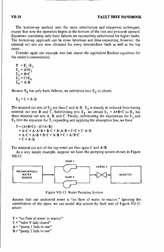
VII-18 FAULT TREE HANDBOOK
The bottom-up method uses the same substitution and expansion techniques,except that now the operation begins at the bottom of the tree and proceeds upward.Equations containing only basic failures are successively substituted for higher faults.The bottom-up approach can be more laborious and time-consuming; however, theminimal cut sets are now obtained for every intermediate fault as well as the topevent.
Consider again our example tree (we repeat the equivalent Boolean equations forthe reader's convenience).
T =E 1 E2El = A+E 3E3 = B+CE2 = C+E4E4 = A.B
Because E4 has only basic failures, we substitute into E2 to obtain
E2= C + AB.
The minimal cut sets of E 2 are thus C and A B. E3 is already in reduced form havingminimal cut sets B and C. Substituting into El, we obtain E1 = A+B+C so El hasthree minimal cut sets A, B, and C. Finally, substituting the expressions for E1 andE2 into the equation for T, expanding and applying the absorption law, we have
T = (A+B+C) • (C+A-B)= A-C + AA'B + B'C + BA'B + C-C + C'A-B= A.C + A.B + B'C + A'B + C + A'B'C= C + AB.
The minimal cut sets of the top event are thus again C and A'B.As a very simple example, suppose we have the pumping system shown in Figure
VII-l 2.
PUMP 1
VALVE V
INEXHAUSTABLEWATER REACTORSOURCE PUMP 2
Figure VII-12. Water Pumping System
Assume that out undesired event is "no flow of water to reactor." Ignoring thecontribution of the pipes, we can model this system by fault tree of Figure VII- 11where:
T = "no flow of water to reactor"C = "valve V fails closed"A = "pump 1 fails to run"B = "pump 2 fails to run"

BOOLEAN ALGEBRA AND APPLICATION TO FAULT TREE ANALYSIS VII-19
We have just shown that the minimal cut sets of this tree are C and A-B. This tellsus that our undesired event "no flow of water to tank" will occur if either valve Vfails closed or both pumps fail to run. In this simple case, the cut sets do not reallyprovide any insights that are not already quite obvious from the system diagram. Inmore complex systems, however, where the system failure modes are not so obvious,the minimal cut set computation provides the analyst with a thorough and systematicmethod for identifying the basic combinations of component failures which cancause an undesired event.
For smaller fault trees, the determination of the minimal cut sets, using either thetop-down or bottom-up method, can be done by hand. For larger trees, variouscomputer algorithms and codes for fault tree evaluation are available. These arediscussed in Chapter XII.
Minimal Path Sets and Dual Fault Trees
The top event of a fault tree represents system failure. This event is of greatinterest from the point of view of system safety. From the point of view of reliabilitywe would be more concerned with the prevention of the top event. Now we knowthat the top event of a fault tree may be represented by a Boolean equation, andbecause this equation may be complemented, there is also a Boolean equation for thecomplement (i.e., nonoccurrence) of the top event. This complemented equation, inturn, corresponds to a tree which is the complement of the original tree. Thiscomplemented tree, called the dual of the original fault tree, may be obtained direct-ly from the original tree by complementing all the events and substituting OR-gatesfor AND-gates and vice versa. In either case, whether we complement the top eventequation or the tree itself, we are applying de Morgan's theorem given in our Tableof Boolean Algebra Laws. The minimal cut sets of the dual tree are the so-called"minimal path sets" of the original tree, where a minimal path set is a smallestcombination (intersection) of primary events whose non-occurrence assures thenon-occurrence of the top event.
The combination is a smallest combination in that all the primary eventnonoccurrences are needed for the top event to not occur; if any one of the eventsoccurs then the top event can occur. The minimal path set expression for the topevent T can be written as
T'=P1 +P 2 +..- +Pk
where T' denotes the complement (nonoccurrence) of T. The terms P1 , P2. .... P,are the minimal path sets of the fault tree. Each path set can be written as
Pi = XfI' •f 2 • '
where the Xi are the basic events in the fault tree and the X'i are the complements.We can find the minimal path sets of a given tree by forming its dual and then
using either the top-down or bottom-up method to find its minimal cut sets. Thesecut sets are the minimal path sets of the original tree which we desire.
Alternatively, if the minimal cut sets of the tree have already been determined, wecan take the complement of the minimal cut set equation and obtain the minimal

VII-20 FAULT TREE HANDBOOK
path sets directly. For our sample tree, we obtained the following minimal cutexpression in the previous section,
T=C+A'B.
Taking the complement
T' = (C + A B)'= C'. (A.-B)'
using de Morgan's theorem. Applying de Morgan's theorem to the term (A- B)'
T' = C"-(A'+B')
and using the distributive law (i.e., expanding)
T' ='C? A' + C" B'
Therefore, the minimal path sets of the tree are C'A' and C'-B'. In terms of ourpumping system of Figure VII-12, this tells us that we can prevent the undesiredevent and assure system success if either
(1) Valve V is open and pump 1 is running, or(2) Valve V is open and pump 2 is running.

CHAPTER VIII - THE PRESSURE TANK EXAMPLE
1. System Definition and Fault Tree Construction
In this and the next chapter, we are going to define undesired events for twosimple systems. The reader will then be shown how the corresponding fault trees aredeveloped step-by-step with the help of the rules described in Chapter V. From thetrees so constructed, some obvious conclusions will be drawn, but detailed evaluationprocedures will be postponed until Chapter XI.
Consider now Figure VIII-I which shows a pressure tank - pump-motor device andits associated control system. First we present details of system operation. Theoperational modes are given in Figure VIII-2.
r --------
RELAYVAE
K1(
RELAY TIMER SIC
Si
FROM RESERVOIR
Figure VIII-1. Pressure Tank System
The function of the control system is to regulate the operation of the pump. Thelatter pumps fluid from an infinitely large reservoir into the tank. We shall assumethat it takes 60 seconds to pressurize the tank. The pressure switch has contactswhich are closed when the tank is empty. When the threshold pressure has beenreached, the pressure switch contacts open, deenergizing the coil of relay K2 so thatrelay K2 contacts open, removing power from the pump, causing the pump motor tocease operation. The tank is fitted with an outlet valve that drains the entire tank inan essentially negligible time; the outlet valve, however, is not a pressure relief valve.When the tank is empty, the pressure switch contacts close, and the cycle is repeated.
Initially the system is considered to be in its dormant mode: switch S1 contactsopen, relay K1 contacts open, and relay K2 contacts open; i.e., the control system is
VIII-I

VIII1-2 FAULT TREE HANDBOOK
ooE
- a -
.444. 4...

PRESSURE TANK EXAMPLE VIII-3
de-energized. In this de-energized state the contacts of the timer relay are closed. Wewill also assume that the tank is empty and the pressure switch contacts are thereforeclosed.
System operation is started by momentarily depressing switch SI. This appliespower to the coil of relay KI, thus closing relay Ki contacts. Relay KI is nowelectrically self-latched. The closure of relay K1 contacts allows power to be appliedto the coil of relay K2, whose contacts close to start up the pump motor.
The timer relay has been provided to allow emergency shut-down in the event thatthe pressure switch fails closed. Initially the timer relay contacts are closed and thetimer relay coil is de-energized. Power is applied to the timer coil as soon as relay K1contacts are closed. This starts a clock in the timer. If the clock registers 60 secondsof continuous power application to the timer relay coil, the timer relay contactsopen (and latch in that position), breaking the circuit to the Ki relay coil (previouslylatched closed) and thus producing system shut-down. In normal operation, when thepressure switch contacts open (and consequently relay K2 contacts open), the timerresets to 0 seconds.
For our undesired event let us take:
RUPTURE OFPRESSURE TANK
AFTER THE STARTOF PUI•P1NG
It will simplify things considerably if we agree to neglect plumbing and wiringfailures and also all secondary failures except, of course, the one of principal interest:"tank rupture after the start of pumping."
The reader may object that a system that includes an infinitely large reservoir andan outlet valve that drains the tank in a negligible time is unrealistic-and now we aresuggesting the neglect of plumbing and wiring faults that might contribute to theoccurrence of the top event. The point is that with this simplified system we canillustrate most of the important steps in fault tree construction. In a more complexsystem the reader might tend to lose sight of the overall system and become tooinvolved in the details.
First we check to make sure that our top event is written as a fault and that itspecifies a "what" and a "when." Next we apply our test question: "Can this faultconsist of a component failure?" Because the answer is "Yes," we immediately addan OR-gate beneath the top event and consider primary, secondary, and commandmodes.* Our tree has now developed to the point shown in Figure VIII-3.
In this problem we shall establish our limit of resolution at the "componentfailure level." By "component" we shall mean those items specifically named inFigure VIII-1. Thus the primary failure of the tank (e.g., a fatigue failure of the tankwall) is already at the limit of resolution and is shown in a circle. Whether or not weinclude the statement in the diamond is moot. We could just assume at the beginningthat the tank was an appropriate one for the operating pressures involved. At anyrate, we choose not to trace this fault any further.
*In this case, however, there is no command mode.

VIII-4 FAULT TREE HANDBOOK
RUPTURE OF PRESSURETANK AFTER THE
START OF PUMPING
TANK RUPTURE RUT~URERPUESDET
(SECONDARY FAILURE) IMROE (PRMLEAICTuAREN
Figure VIII-3. Fault Tree Construction - Step I
Thus our attention is now directed to the secondary failure of the tank. Thereader will remember from Chapter V, that in contrast to a primary failure, which isthe failure of a component in an environment -for which it is qualified, a secondaryfailure is the failure of a component in an environment for which it is not qualified.Because the secondary failure of the tank can consist of a component failure, weintroduce another OR-gate and our tree assumes the form shown in Figure VIII-4.
Here again we indicate, in a diamond, a set of conditions whose causes we choosenot to seek. Notice that the fault spelled out in the rectangle is a specific case of thetop event with a more detailed description as to cause.
Now it might happen that our tank could miraculously withstand continuouspumping for t > 60 seconds but an application of our "No Miracles" rule constrainsus to the statement that the tank will always rupture under these conditions. We canindicate this on the fault tree by using an Inhibit gate whose input is "continuouspump operation for t > 60 seconds" (see Figure VIII-5).
Can the input event to the Inhibit gate consist of a component failure? No, thepump is simply operating and pump operation for any length of time cannot consistof a component failure. Therefore this fault event must be classified "state-of-system." We now recall the rules of Chapter V. Below a state-of-system fault we canhave an OR-gate, an AND-gate, or no gate at all. Furthermore, we look for theminimum, immediate, necessary and sufficient cause or causes. In this case theimmediate cause is "motor runs for t > 60 seconds," a state-of-system fault. Itsimmediate cause is "power applied to motor for t > 60 seconds," a state-of-systemfault. The immediate cause of the latter event is "K2 relay contacts remain closed fort > 60 seconds." We have now added the string of events shown in Figure VIII-6.
In this case, nothing is lost by jumping from "pump operates continuously fort > 60 seconds" directly to "K2 relay contacts remain closed for t > 60 seconds."There is, however, no harm done in detailing the intermediate causes and, as a matterof fact, the opportunity for error is lessened thereby.

PRESSURE TANK EXAMPLE VIII-5
TANK RUPTURE
(SECONDARY FAILURE)
TANK RUPTURES DUE TOINTERNAL OVER-PRES- TANK FAIL OMSURE CAUSED BY CON- OTHER OUT-OF-TOLERANCETINUOUS PUMP OPERA- CONDITIONS (e.g.,TION FOR t > 60 SEC TEML
Figure VIII-4. Fault Tree Construction - Step 2
TANK RUPTURES DUETO INTERNAL OVER-
PRESSURE CAUSED BYCONTINUOUS PUMP
OPERATION FORt>60SEC
PUMP OPERATESCONTINUOUSLYFOR t >60 SEC
Figure VIII-5. Fault Tree Construction - Step 3

VIII-6 FAULT TREE HANDBOOK
PUMP OPERATESCONTINUOUSLYFOR t >60 SEC
MOTOR RUNSFOR t > 60 SEC
IPOWER APPLIED
TO MOTO RFOR It>60 SEC
IK2 RELAY CONTACTS
REMAIN CLOSEDFOR t > 60 SEC
Figure VIII-6. Fault Tree Construction - Step 4
We have now to consider the fault event, "K2 relay contacts closed for t > 60seconds." Can this consist of a component failure? Yes, the contacts could jam, weld,or corrode shut. We thus draw an OR-gate and add primary, secondary, andcommand modes as shown in Figure VIII-7.
The event of interest here is the command mode event described in the rectangle.Recall that a command fault involves the proper operation of a component, but inthe wrong place or at the wrong time because of an erroneous command of signalfrom another component. In this case, the erroneous signal is the application of EMFto the relay coil for more than 60 seconds. This state-of-system fault can be analyzedas shown in Figure VIII-8.
Notice that both input events to the AND-gate in Figure VIII-8 are written asfaults. In fact, as we know, all events that are linked together on a fault tree should

PRESSURE TANK EXAMPLE VIII-7
K2 RELAY CONTACTSREMAIN CLOSEDFOR t> 60 SEC
2 EMF APPLIED TO
(SECONDARY CONTACTS FAILTO OPENK2 RELAY COILFAILRE)(PRIARYFOR t •> 60 SEC
Figure VIII-7. Fault Tree Construction - Step 5
EMF APPLIED TOK2 RELAY COILFOR t > 60 SEC
EMF REMAINS ONPRESSURE SWITCH PRESSURE SWITCHCONTACTS CLOSED CONTACTS WHEN
FOR t •> 60 SEC PRESSURE SWITCHCLOSED FOR t >60SEC
Figure VIII-8. Fault Tree Construction - Step 6
be written as faults except, perhaps, those statements that are added as simplyremarks (e.g., statements in ellipses). The pressure switch contacts being closed is nota fault per se, but when they are closed for greater than 60 seconds, that is a fault.Likewise the fact that an EMF is applied to the pressure switch contacts is not itself afault. Notice that the condition that makes this event a fault is framed in terms ofthe other input event to the AND-gate.
The fault event, "pressure switch contacts closed for t > 60 seconds," can consistof a component failure, so both input events in Fivure VIII-8 are followed byOR-gates. We analyze them separately, starting with tie left-hand event (see FigureVIII-9.

VIII-8 FAULT TREE HANDBOOK
PRESSURE SWITCHCONTACTS CLOSED
FOR t >60SEC
SNEBYPRESSURENO SWITCH CONTACTS PRESSURE SWITCHSESDB RSUEFAIL TO OPEN (SECONDARY
Figure VIII-9. Fault Tree Construction - Step 7
We see that this leg of the tree has reached its terminus (all input events are eithercircles or diamonds) unless, for some reason, we wish to pursue the event in theleft-hand diamond somewhat further (e.g., ruptured diaphragm, etc.).
We now analyze the right-hand event in Figure VIII-8 as shown in Figure VIII-10.Both the input events in Figure VIII-IO are state-of-component faults. The
left-hand one is the more easily analyzed as shown in Figure VIII-1 1.
EMF REMAINS ON PRES-SURE SWITCH CONTACTSWHEN PRESSURE SWITCHCONTACTS CLOSED FOR
t>60 SEC
EMF THRU KI RELAY EMF THRU - SWITCHCONTACTS WHEN PRES. CONTACTS WHEN PRES-
SURE SWITCH CONTACTS SURE SWITCH CONTACTSSCLOSED FOR > >60 SEC CLOSED FOR t > 60 SEC
Figure VII[-I 0. Fault Tree Construction - Step 8

PRESSURE TANK EXAMPLE VII-9
EMF THRU Si SWITCH
CONTACTS WHEN PRES-SURE SWITCH CONTACTSCLOSED FOR t>60SEC
FORCE REMAINS ON TO OPEN (EODR
Figure VIII-1 1. Fault Tree Construction - Step 9
Here we have reached another tree terminus. The analysis of the remaining inputevent in Figure VIII-10 is shown in Figure VIII-12. The reader will note from thislatter figure that we have finally worked our way-in this step-by-step fashion-downto timer relay faults. Finally, we show the complete fault tree for the pressure tankexample in Figure VIII-l 3.
Actually, the fault tree of Figure VIII-13 could be considered too complete.Because the only secondary failure that we developed was the rupture of the pressuretank due to overpumping, other secondary failures (the dotted diamonds) couldsimply be omitted from the diagram. Further simplifications can also be made,leading to the basic fault tree of Figure VIII-14, where the circles represent primaryfailures as shown in the legend and the fault events El, E2 etc. are defined asfollows:
The E's are fault events.
El - Pressure tank rupture (top event).E2 - Pressure tank rupture due to internal overpressure from pump
operation for t > 60 seconds which is equivalent to K2 relay contactsclosed for t > 60 seconds.
E3 - EMF on K2 relay coil for t > 60 seconds.E4 - EMF remains on pressure switch contacts when pressure switch
contacts have been closed for t > 60 seconds.E5 - EMF through KI relay contacts when pressure switch contacts have
been closed for t > 60 seconds which is equivalent to timer relaycontacts failing to open when pressure switch contacts have been closedfor t > 60 seconds.

VIII-10 FAULT TREE HANDBOOK
EMF THRU K1 RELAYCONTACTS WHEN PRES-
SURE SWITCH CONTACTSCLOSED FOR >60 SEC
IEMF NOT REMOVED FROMIKI KRELAY COIL WHEN K1] RESSURE SWITCH FALT PNIEODR
ICONTACTS CLOSED (PIAYFIUE[ FORt >60OSEC FAL M;
TIMER RELAY CONTACTSFAIL TO OPEN WHEN
PRESSURE SWITCHCONTACTS CLOSED
FOR t > 60 SEC
TIME
FiguES NOT1.FutTreCntuton-FnlSe

PRESSURE TANK EXAMPLE
U,-u
==w
-- -u
w- ow
VU--u-
Zo1'
VV
Figure VIII-I 3. Pressure Tank Rupture Fault Tree Example

AA
L ~ )
V;
L4A
.Figure~~~~~~ ~ ~ ~ ~ ~ ~ VIII3 AsueTn utr al reEanl

VIIi-12 FAULT TREE HANDBOOK
2. Fault Tree Evaluation (Minimal Cut Sets)
Fault tree evaluation in general will be taken up in Chapter XI. It is useful at thispoint, however, to evaluate the fault tree so that we can assess, in a gross way, thestrengths and particularly the weaknesses of the pressure tank control circuit.
From the basic fault tree of Figure VIII-14 we can express the top event as aBoolean function of the primary input events using the method explained in ChapterVII. This is accomplished by starting at the top of the tree and working down:
El = T + E2= T+(K2+E3)= T+K2+(S. E4)= T+K2+S'(SI+EE5)= T+K2+(S. Sl)+(S E5)= T+ K2+(S. SI)+S (KI + R)= T+ K2 + (S • Sl)+ (S • KI) + (S • R)
This expression of the top event in terms of the basic inputs to the tree is theBoolean algebraic equivalent of the tree itself. El appears as the union of variouscombinations (intersections) of basic events and is the minimal cut expression for thetop event. In our example, we have found five minimal cut sets-two singles andthree doubles:
K2TS-S1S. KIS.R
Each of these defines an event or series of events whose existence or joint existencewill initiate the top event of the tree.
We are now in a position to make, first, a qualitative assessment of our results andthen, armed with some data, a gross quantitative assessment. Qualitatively, theleading contributor to the top event is the single relay K2 because it represents aprimary failure of an active component. Therefore, the safety of our system wouldbe considerably enhanced by substituting a pair of relays in parallel for the singlerelay K2. Actually, however, our system contains a much more serious design error:We are monitoring the controls instead of the parameter of interest (pressure in thiscase). It should be just the other way around! Thus, the most obvious way toimprove the system would be to install a pressure relief valve on the tank and removethe timer.
The next basic event, in order of importance, is T, the primary failure of thepressure tank itself. Because the tank is a passive component, recall from Chapter Vthat the probability of the event T should be less (by an order of magnitude or so)than the probability of event K2. Of less importance are the three double componentcut sets S-SI, S.KI, and S.K2, although we do note that the failure of the pressureswitch contributes to each of them.
To make a quantitative assessment of our results we need estimates of failureprobabilities for our components. Table VIII-I gives values for the failureprobabilities for the components in the system. The calculations involved in gettingthese numbers will be discussed later; at this time we simply assume the values asbeing "data."

PRESSURE TANK EXAMPLE VMl-13
El
rM 2
si E5
LEGEND: FAULTS K1
El TOP EVENT
E2, E3, E4, E5 INTERMEDIATE FAULT EVENTS
R PRIMARY FAILURE OF TIMER RELAY
S PRIMARY FAILURE OF PRESSURE SWITCH
Si PRIMARY FAILURE OF SWITCH S1
K1 PRIMARY FAILURE OF RELAY K1
K2 PRIMARY FAILURE OF RELAY K2
T PRIMARY FAILURE OF PRESSURE TANK
Figure VIII-14. Basic (Reduced) Fault Treefor Pressure Tank Example

VHI-14 FAULT TREE HANDBOOK
Table VIII-I. Failure Probabilities for Pressure Tank Example
COMPONENT SYMBOL FAILURE PROBABILITY
Pressure Tank T 5 x 10⁻⁶
Relay K2 K2 3 x 10⁻⁵Pressure Switch S I x 10-4
Relay K1 KI 3 x 10⁻⁵Timer Relay R 1 x 10⁻⁴
Switch S I S1 3 x 10⁻⁵
Because a minimal cut is an intersection of events, the probabilities associatedwith our five minimal cut sets are obtained by multiplying the appropriatecomponent failure probabilities (assuming independence of failures);
P[T] = 5 x 10⁻⁶P[K2] = 3 x 10⁻⁵P[S- K1] = (1 x 10⁻⁴) (3 x 10⁻⁵) = 3 x 10⁻⁹P[S- R] = (l X 10-4) (1 X 10⁻⁴)= l x 10-8P[S- S1] = (1 x 10⁻⁴) (3 x 10⁻⁵) = 3 x 10⁻⁹
We now wish to estimate the probability of the top event, El. Observing that thetop event probability is given by the probability of the union of the minimal cut sets,and that the probability of each individual minimal cut set is low, we conclude thatthe rare event approximation of equation (VI-7) is applicable. We therefore simplysum the minimal cut set probabilities and obtain:
P(E 1)- 3.4 x 10 -5
The relative quantitative importance of the various cut sets can be obtained bytaking the ratio of the minimal cut set probability to the total system probability:
Cut Set Importance
T 14%K2 86%S • R Less than 0.1%S-SI
The pressure tank example has been provided on numerous occasions as aworkshop exercise for students learning the basics of fault tree construction. Themost frequent analytical error made by these students is the tendency to leapdirectly from the event of rupture to the pressure switch. When this is done the singlefailure minimal cut set K2, i.e., the primary failure of K2, is missed completely. Thisillustrates the importance of applying the rules described in Chapter V.
One design-related principle that arises out of this example is that a system shouldbe designed so that AND-gates appear as close to the tree-top as possible in an effortto eliminate single event cut sets. The family automobile is a good example of asystem which is not of this type, and the reader can amuse himself by making alengthy list of single events that will immobilize his car.

CHAPTER IX - THE THREE MOTOR EXAMPLE
1. System Definition and Fault Tree Construction
In this chapter we discuss a somewhat more complicated example of fault treeconstruction and evaluation.* Figure IX-1 displays a power distribution box andFigure IX-2 gives the system modus operandi. With contacts KT1, KT2, and KT3normally closed, a momentary depression of pushbutton Si applies power fromBattery 1 to the coils of cut-throat relays KI and K2. Thereupon KI and K2 closeand remain electrically latched.
TEST SIGNAL
I I
iATTERYtrT
ETI KT2 KT3 I
BATTERY 2
Figure IX-l. Power Distribution Box Fault Tree Example
Next, a 60-second test signal is impressed through K3, the purpose being to checkthe proper operation of Motors 1, 2, and 3. Once K3 has closed, power from Battery1 is applied to the coils of relays K4 and K5. The closure of K4 starts Motor 1. Theclosure of K5 applies power from Battery 2 to the coil of K6 and also starts Motor 2.Finally, the closure of K6 applies power from Battery 1 to the coil of K7. Closure ofK7 starts Motor 3.
After an interval of 60 seconds, K3 is supposed to open, shutting down theoperation of all three motors. Should K3 fail closed after the expiration of 60seconds, all three timers (KTI, KT2, KT3) open, de-energizing the coil of Ki, thusshutting down system operation. Suppose K3 opens properly at the end of 60seconds, but K4 fails closed. In that case KT1 opens to deenergize K1 and Motor 1stops. KT2 and KT3 act similarly to stop Motor 2 or Motor 3 should either K5 or K7fail closed.
*For an actual example of a fault tree analysis applied to a major nuclear safety system seeU.S. Nuclear Regulatory Commission, "Reactor Safety Study-An Assessment of Accident Risksin U.S. Commercial Nuclear Power Plants," WASH-1400 (NUREG-75/014), Appendix II, "FaultTrees," Section 2, "Fault Tree Analysis."
IX-1

IX-2 FAULT TREE HANDBOOK
20 20. 2-3l--
z0 i
uj cc 009i uw w n W m If w be -cc *u
3: be~
0 u', C3
2~~~~ en-o ~..Jou '- cc
E w~0 w0
0
w i-o.;- b-s 1-1 P 0 4.. 4,. 0
o 0'- w ~ 0 20 10
0 , 00 0 1.0
4 -- 0
(4 z
II-
zO ~ 0
0~ i-L0
I -
(4 L 4

THREE MOTOR EXAMPLE IX-3
OVERRUN OF ANYMOTOR AFTER
TEST IS INITIATED
EMF APPLIED EMF APPLIED EMF APPLIEDTO MOTOR I TO MOTOR 2 TO MOTOR 3
FOR t > 60 SEC FOR t > 60 SEC FOR t > 60 SEC
A AFigure IX-3. "Treetop" for Motor Overrun Problem
Our main concern in this problem is the "overrun" (t > 60 seconds) of any one ofthe motors after test initiation. Thus our "tree top" appears as in Figure IX-3.
Each of the three inputs to the OR-gate must be analyzed separately. We proposeto treat the overrun of Motor 2 first. To avoid a clutter of trees on a single sheet,"transfer out" symbols, as shown, are applied to the fault events relevant to Motor 1and Motor 3.
At this point, we have to decide how exhaustive our analysis is going to be. Thesimplest approach would be to restrict ourselves to the failures of relays andswitches, and we shall do this first. A fuller analysis (which we shall hold in abeyancefor awhile) would also include possible wiring defects. Limiting the analysis to theformer problem for the moment, we are faced with the top event:
EMF APPLIEDTO MOTOR 2
FOR t >60 SEC
Because this is a state-of-system fault, we look for immediate necessary andsufficient causes. We see from Figure IX- 1 that two fault events have to exist to causethe occurrence of the event of interest:
(1) K5 relay contacts remain closed for t > 60 seconds.(2) K2 relay contacts fail to open when K5 relay contacts have been closed for
t > 60 seconds.

IX-4 FAULT TREE HANDBOOK
These two fault events are shown as inputs to the 2nd level AND-gate in Figure IX-4which displays the completed tree for overrun of Motor 2. Notice that the failures ofK5 or K2 contacts to open are not, of themselves, faults; they become faults.however, when the time restriction is specified.
We now direct our attention to the fault event:
K5 RELAY CONTACTSREMAIN CLOSEDFOR t>60 SECS.
T 0.11100
Figure IX4. Fault Tree for Overrun of Motor 2 (Relay Logic Only)
Because this is a state-of-component fault, it demands an OR-gate with primary,secondary, and command inputs. To simplify the problem, let us not pursuesecondary failures. Thus, Figure IX4 shows only primary and command inputs. Theprimary failure of K5 relay is already a basic tree input (a limit of resolution); weturn our attention therefore, to the command input which is

THREE MOTOR EXAMPLE IX-$
EMF REMAINSON K5 COIL
FOR t > 60 SEC
We note that this event is a state-of-system fault. From Figure IX-I we find that thisfault event will occur when both K3 contacts and K 1 contacts fail to open with thetime restriction t > 60 seconds. These two events are shown in Figure IX4 as inputsto the 4th level AND-gate on the left. The fault event relevant to relay K3 is astate-of-component fault which demands an OR-gate followed by primary andcommand inputs. In this case, the command input is shown in a diamond because itscause (or causes) lie "outside" of our defined system. This leg of the tree is nowcomplete.
Returning now to the fault event relevant to KI relay, we realize that it will bethe "top event" of a fairly substantial subsidiary tree of its own. We therefore"transfer out" to another sheet of paper (see Figure IX-5). As a matter of fact, thisstrategy proves to be particularly useful inasmuch as this same fault event recurs inthe analysis of the overruns of Motor I and Motor 3. The task of studying the detailsof the subsidiary fault tree of Figure IX-5 is left to the reader.
Referring once more to Figure IX-4, we now have to consider the righthand inputto the 2nd level AND-gate. This fault event is
K2 RELAY CONTACTSFAIL TO OPEN WHEN
K5 RELAY CONTACTSCLOSED FOR t> 60SEC
This is a state-of-component fault whose command input is
EMF NOT REMOVEDFROM K2 RELAY COIL
WHEN K5 RELAYCONTACTS CLOSED
FOR t> 60 SEC
a state-of-system fault. This is really a single input event except that we have alsochosen to consider the possibility (highly improbable) of an EMF on the K2 coilthrough the S I, KTI, KT2 and KT3 contacts. This latter event appears in a diamondin Figure IX-4.
The details of the rest of the right leg of the tree are left to the reader. The basic-. inputs are primary failures of KI relay, S 1 switch and KT2 timer contacts.

Ix.'
Ki RELAY CONTACTS
FAIL TO OPEN WHENK3 CONTACTS CLOSED
FOR t 60 SEC
SEMF NOT REMOVED
KI RELAYFROM KI1RELAYCONTACTSCOIL WHEN K3FAIL TOCONTACTS CLOSED
OPEN FOR t *60 SEC
EMF TO K1 COILTHRU TIMER
CIRCUIT WHENK3 CONTACTS CLOSED
FOR 1>60 SEC
KT1 TIMER CONTACTS KT2 TIMER CONTACTS KT3 TIMER CONTACTSFAIL O OPN FAL TOOPENFAIL TO OPEN
WHEN K3 CONTACTS WHEN K3 CONTACTS WHE N K3 CONTACTSCLOSED FOR t>S0SEC CLOSED FORt >60SEC CLOSED FOR: -60SEC
TKMERKTKTCONTACTS FAIL • ,DOES NOT "TIME OUT" DOSNT iEor0OT0S ALOESNOTI
FAILPN DU TOOMPROER , DUE TO
Figure IX-5. Analysis of Fault Event Relevant to K1 Relay

FAULT TREE HANDBOOK
K RELAY CNTACTSFAl. TO OPEN WHEN
K3 CONTACTS CLOSEDFOR F> 60 SEC
SEMF NOT REMOVED
KI RELAYFROM K1RELAYLCOIL WHEN K3
WNCONTACTS CLOSEDFORC FR SEC
R
EMF TO KI COIL NFTK CITHRU TIMER E FTOA S1 CONT CT
CIRCUIT WHEN WHEN K3 CONTACTSK3 CONTACTS CLOSED CLOE D FOR >CONTA CT
FOR t •> 60 SEC COE O • 0E
DT IE OESNOTACTIM OUT DIE OESNOATS 'IEOT
FAIL TO OPEN FAIL TO OPENS1WICWHEN K3 CONTACTS WHE N K3 CONTACTSINDETTL STIGA
CLOSED FOR > 60 SEC C LOSED0 FO0R I 1M60 SECCLSSOINDETTY
ENOUE TO IMPROPER OUE TO IMPROPER SINSTALLATION TR INSTALLATION ORSETTN 3ETTIMNE
Figure IX-5. Analysis of Fault Event Relevant to KI Relay
0ItET F E

THREE MOTOR EXAMPLE IX-7
The fault trees relevant to overruns of Motor 1 and Motor 3 are shown in FiguresIX-6 and IX-7. A more exhaustive study of the overrun problem for Motor 2(including wiring defects) is shown in Figures IX-8, and IX-9. The reader may nowcare to try his hand at the analysis of a different top event: Motor 1 fails to start inpresence of test signal. A solution for Motor 1 is displayed in Figure IX-lO.
2. Fault Tree Evaluation (Minimal Cut Sets)
We now turn to the qualitative evaluation of the fault tree of Figure IX-4 anddetermine the minimal cut sets for the overrun of Motor 2. For ease of presentationwe will deal with a reduced version of the fault tree of Figure IX-4 where thediamonds ind houses are removed. The reduced tree is shown in Figure IX-I 1.
In Figure IX-i1 the circles represent primary failures of the components denoted,and the fault events E1 , E2 , etc. are defined as follows:
E1 - EMF applied to Motor 2 for t > 60 seconds.E2 - K5 relay contacts remain closed for t > 60 seconds.E3 - K2 relay contacts fail to open when K5 contacts have been closed
to t > 60 seconds.E4 - EMF remains on K5 coil for t > 60 seconds.E5 - KI relay contacts fail to open when K5 contacts have been closed for
t > 60 seconds.E6 - K1 relay contacts fail to open when K3 contacts have been closed for
t > 60 seconds.E7 - EMF not removed from Ki relay coil when K3 contacts have been
closed for t > 60 seconds.
The reader should note that events E5 and E6 , although similar, are not the samebecause the "when" is different. Thus, the tendency to transfer the fault event E5 tothe subsidiary tree of Figure IX-5 must be strongly resisted.
In the equations below each fault event is expressed in terms of its equivalentBoolean equation. Engineering notation is used.
El = E 2 • E3E2 = K5 + E4E3 = K2 +E5E4 = K3. E6E5= KI+KT2+SlE6 = Kl + E7 + SlE7= KTl . KT2 " KT3
Next, starting from the bottom of the tree, each fault event is expressed in terms ofthe basic tree inputs.
E7 =KTI" KT2"KT3E6 = KI +(KT1 - KT2 - KT3)+ SlE5 =K1 + KT2 +Sl

IX-8 FAULT TREE HANDBOOK
E4 =K3 • (Ki + KT1 • KT2 • KT3 + Sl)=K3 KI +K3 (KT1 "KT2 KT3)+K3 Si
E3 =K2+KI +KT2+S1E2 = K5 + K3 • KI + K5 + K3 • (KT1 • KT2 • KT3) + K5 + K3 • S1El = [K5 + K3 KI + K5 + K3 (KTI KT2 KT3) + K5 + K3 SI]
- [K2 +Kl+ KT2 +S1]
The Boolean expression for E1 simplifies to:
El = {KS + (K3. KI) + [K3 (KTI • KT2 KT3)] + (K3 .SI)}- {K2+ K1 + KT2 +S1)
Expanding this expression using the distributive law, the minimal cut sets (allredundancies eliminated) are:
K5 K2K5 KIK5 KT2KS SIK3 KIK3 SIK3 KTI KT2 • KT3
Note, for instance, that because (K3. K1) is minimal from the relationship(K3 • KI • K1)= (K3 • K1), then (K3 • KI • K2), for example, is not minimal.
All the minimal cut sets above are "doubles" except the last one which appears tobe a "quadruple." If all three timers, however, are identical, they might be likelycandidates for a so-called "common case" failure. In this case, our ostensiblequadruple minimal cut set becomes essentially a "double." In later sections, we willfurther discuss common cause failures.
The reader should now try his hand at identifying the minimal cut sets in theother two problems: overrun of Motor I and overrun of Motor 3. Following theprocedure detailed for Motor 2 he should be able to check the following solutions:
MINIMAL CUT SETS MINIMAL CUT SETS
(Overrun of Motor 1) (Overrun of Motor 3)
K1 • K4 K1 - K7K4 - S1 K2 K7K4.KTI K7 KT3KI K3 K7 SIK3 • Sl KI K3
K3 • KTI • KT2 • KT3 K3 S1K3 KTI KT2 KT3

THREE MOTOR EXAMPLE
REAIN APLOSED
X4 RELAY CONTACTSKFOR t > SO SEC
EMF RMAINSEMFI NOT REMOVED
00 KACOILKII ELAYFROM Ki RELAV
FOR COIL WHEN K4I > SECCONTCTSCONTACTS CLOSED
FOR 6-'SSEC
ElRLYCOTCS 9 RELAY CONTACTS EMEF TO KNI COILK3REMAYN CLONTACT FAIL TO OPEN THRU SI CONTACTS
WHEN IIICONTACTS WHEN III CONTACTSCLOSED FOR I> S'... CLOSED FO R i> 60SEC
SIGNAL REMAINS CONTACTS INADVERTENTLYINDETTL
Figure IX-6. Fault Tree for Overrun of Motor I (Relay Logic Only)

IX-9
SED FAIL TO OPEN
RESET5 SIIRLANCNTLTSE, ETNLYIAVRENL IE WHEN K4CN CT TONTAET
CPLOSED ORR 60SE
REMVE PROMEMVESWTC REASIM EA
CONTAultTre forL OWerru of Moto 1RReayLoAcOYy

IX-1O
IMF AMPLIESTO MOTO )
1 O a[sic
? RE Y CONTACTSCO FAL ToO S
FO~lC1OO s FORI , "CO
REMAIN CLOSED W:I. C T
FOR~~~~~~LOE '0.'SC ;OIO rnI> O[
fop -G S[C.'I COOT
ONEll TO El COI L
CLO ~ ~ COSE FOR , l[
IMFE 011 ISI U E
I~~~~0 TRSCI CESAT CONTACTS
FIg oMo TO TOla o l)
COTAT CONACT Ios PPLIFoFAI TOD TO III CONTASO
WHI FR IS
Figur
A"
F
To I

FAULT TREE HANDBOOK
IMF WPPIND
TO MOTOR]I
WHA COOTLCT
WHE ITCONACT
CLSE FRI U E
.NACTS COTCSOI n
I A 0 IAIOR I o TCSCOE
FIgur gnu FFult Tra >o Ovru"otoori(elyLgicny
©lRLYCNAT

THREE MOTOR EXAMPLE
I!E2:
-E5i
Figure D(-8. Fault Tree for Overrun of Motor 2 (Including Wiring Defects

IXC-11
.1 3
V5j5
- :2
-8.~ Fal refrOvru fMtr IcuigWiigDfcs

.IX-12
EM' IEMAIMSAVAILA: LE TO AT
CONTACTS WHIEN K3CONTAtCtS COS ED
FO So M SEC
IMF TO XI COITCT FAULT`S
CIRUI CE Eo L I 'HITIECONTACTSECLOSES CIRCUITRY
CLOSE FOR Go
FEM IIIIREAY ONTC3TEOR DOES RT TIME OUTSUER OSES OT TI.E OS T IO E OOSNn IMRAIL T INSTLLATIN SR AIL 5 INSTLLATIN OR A I TOISALAINS
Fiue IX9 Sute orTaserT"iMorOvruPobe
BATR I..X CNAT

FAULT TREE HANDBOOK
IMF faRHINSAIAILABLI T 101
CONTACTSWWII U3CONTACTS CLOSED
OR>19SEC
UHF ~ FO 101 COT1STO U
THOU K1 COSTACTS KI. ITS. K2.123 A KWREN ROICONTACT, WINE CIRCUITRSY
CLOSED FORI I' ?4EC
IF RELAY CONTACTSFAIL TO OPEN
WHER KISCONTACTS
EMF APPFLIED TOEl RELAY a I COIL WHEN 12CONTACTS CONTACT CLOSEDFAIL j TO FOR? NA SEC
FAULTS RU OE lCOITOI A EH IN THO 0 CNTACTS
(£ITIMER 8HU 13Cin ACIRCUITRY CILUEDFUI)SE
Uy I TIMER CUNTACTS * EMF El SWITCH CONTACTSIFAIL TO SPENl FOM CLOSES WIR OKI
CTS IWHENAS CONTACTS ATy ERY I CONTACTS CLOSEDIsJ LOOSI FOR,>OE ALIFR>QE
KTITIME ITS KT3TIHERRET 1SIC
ODU OTTIEOUT TRINE DODES NOT TIME OUT INAADVERTENTALLYUSUE To DWO OTCSGUE TO IMPROFERCLSSOINUSTALLATIO ORFILT INSTA LL ATION URA IT
SETII ON SETTINGSITH11I
Subtree for Transfer "T"l in Motor Overrun Problem

THREE MOTOR EXAMPLE
,~Zia
.Cr n
FiueI-0 FutTe o MotrIFiueoSat

IX13
az
*1 *3
lwg2
igur IXlO.Faul Tre fr Moor Falureto tar

IX-14 FAULT TREE HANDBOOK 1
El|
E2 E3
K1"
Figure IX- 11. Basic Fault Tree for Overrun of Motor 2

CHAPTER X - PROBABILISTIC AND STATISTICAlANALYSES
1. Introduction
In this chapter we shall attempt to present those basic elements that are necessaryfor understanding the probabilistic and statistical concepts associated with the faulttree. This material will also serve as the basis for future chapters on thequantification of fault trees. The reader who feels well-versed in statistics andprobability may prefer to skip this chapter and proceed directly to Chapter XI. Hemay find it convenient at a later time to review this chapter as the need arises.
We shall start with a discussion of probability distribution theory. To introd..cethis discussion we shall first look at the binomial distribution and shall then proceedto distribution theory in general, with emphasis on some specific distributions thatare of special interest to the systems analyst. We shall then attack the basics ofstatistical estimation.
The method of presentation, although perhaps not in the best tradition ofmathematical statistics, has been developed by one of the authors in the course ofteaching statistics to engineering students and engineers in the field. In this processmathematical rigor has sometimes been sacrificed to expedite the explication of basicideas.
2. The Binomial Distribution
Suppose that we have 4 similar systems that are all tested for a specific operatingtime. At the end of each test let us further suppose that the test results allow us tocategorize each run unambiguously as "success" or "failure." If the probability ofsuccess on each run is designated by p (and thus the probability of failure is (l-p)),what is the probability of x = 0, 1, 2, 3, 4 successes 6ut of the four runs or trials?
The outcome collection for this experiment can be easily written down (subscripts'denote run number, and "S" and "F" stand for success and failure):
x =_4 x =.3 x =_2 x =_I1 x--O
S1S2F 3 F4S1 S2 S3 F4 S1 F2 S3 F4 FIF 2 F3 S4
S1S2 S3S4 S1 S2 F3 S4 FIS 2 S3 F4 F1 F2 S3 F4 FIF 2 F 3F4S1 F2 S3 S4 FIS 2 F3 S4 F 1S2 F 3F4
SjF 2 F3 S4F1S2S3 S4 F1 F2 S3S4 S1F2 F3 F4
A symbol such as SIF 2 S3 F4 means, "first run successful, second run a failure, thirdrun successful, fourth run a failure." The probability of this particular outcome isp (l-p) . p (l-p) = p2 . (1-p)2 . Note that in 4 trials, it is possible to have 4
X-I

X-2 FAULT TREE HANDBOOK
successes (x = 4) in only 1 way, 3 successes (x = 3) in 4 ways, 2 success (x = 2) in 6ways, 1 success (x = 1) in 4 ways, and no successes (x = 0) in only I way. In generalfor n trials the number of ways of achieving x successes is
(n) x n!kxx! (n-x)!
which is the number of combinations of n items taken x at a time. Note also thatthere are a total of 16 = 24 outcomes. If there were n trials and each trial could beclassified as "success" or "failure," there would be 2 n outcomes.
Now let us classify these results in a somewhat different way as follows:
No. of Successes No. of Ways Probabilit
x = 0 1 lp 0 (l-p)4
x = 1 4 4pl(-p)3
x=2 6 6p 2(l-p)2
x = 3 4 4p 3(l-p)1
x=4 1 1p4 (l-p)0
Consider the terms in the last column. For example, 4p 3(1-p) represents theprobability of having exactly 3 successes in 4 trials. Three successes in 4 trials canoccur in 4 ways (thus the coefficient 4) and if we have had 3 successes, we must havehad also 1 failure. The probability of a particular outcome of three successes and onefailure is p3(1-p) and because there are 4 possible outcomes in which three successesare obtained the total probability is 4p 3(1-p). These expressions in the last columnrepresent individual terms in the binomial distribution, the general form of which iswritten as follows:
If the probability of success on any trial is p, then
P[exactly x successes in n trials] = (n) pX (lp)n-x(X-l)
-b (x;n,p)
in which b (x; n, p) represents the binomial distribution in what is termed probabilitydensity form. (The probability density form is discussed further in succeedingsections.)* If the reader will set n = 4 and let x range through the values of 0 to 4, hewill see that the individual terms in the probability column of our previous exampleare generated by equation (X-M).
*For a discrete variable such as x, the probability density is also sometimes called theprobability mass function.

PROBABILISTIC AND STATISTICAL ANALYSES X-3
Questions regarding the probabilities of having at most x successes in n trials andat least x successes in n trials can be answered by summing the appropriate individualterms. Thus:
xP[at most x successes in n trials] = E (n) pS(1-p)n-s B(x; n,p) (X-2)s0
nP[at least x successes in n trials] = (n) ps(l -p)n-
S=X
x-1
=1- ) (n)pS(l-p)n-s (X-3)s=O
where B (x; np) is the binomial distribution in cumulative distribution form (thecumulative distribution form is discussed further in upcoming sections). At this stagewe may simply interpret the cumulative binomial as giving the probability that thenumber of successes is less than or equal to some value. Thus, returning to ourexample, the probability of having at least 2 successes in 4 trials is,
6p 2 (l-p)2 + 4p 3 (l-p) + p4 = 1- I(1-p)4 + 4p(l-p)3].
The binomial distribution is extensively tabulated, often in the form of equation(X-2) but also occasionally in the form of equation (X-3) and sometimes in the formof equation (X-l). See for example References [1], [33], and [41].
The statistical average of the binomial distribution is np and its variance isnp(l-p). The average is a measure of the location of the distribution and the varianceis a measure of its dispersion, or spread. These terms are discussed further insubsequent sections.
We have made a number of assumptions (tacitly so far) in our own use of thebinomial. It is of the utmost importance to list these assumptions explicitly:
(1) Each trial has only one of two possible outcomes. We have called these"Success"/"Failure" but they could just as well be called anything else (e.g.,defective/nondefective).
(2) There are exactly n random trials and n is numerically specified.(3) All n trials are mutually independent.(4) The probability of "success" (or whatever you want to call it) on any trial is
designated by some letter such as p, and p remains constant throughout the sequenceof trials.
It is important for the reader to realize that if a problem comes up and one ormore of these assumptions is violated, then use of the binomial distribution will bequestionable unless the effect of the violation is investigated. All distributions and, asa matter of fact, all mathematical formulae are characterized by underlyingassumptions and restrictions, and a valid use of these distributions or formulaeinvolves a knowledge of what the associated assumptions and restrictions are.

X-4 FAULT TREE HANDBOOK
Let us now return to our list of assumptions and consider them in more detail.What can be done in case one or more of these restrictions happens not to be true?We will look at only a few cases to indicate the possible violations to theassumptions.
(1) What if each trial has more than 2 possible outcomes? For instance, in certaintesting methods, 3 decisions are possible after each trial: accept the lot, reject thelot, continue testing. If we are drawing single chips from a container holding amixture of white, green, red, blue, and yellow chips, then each trial has 5 possibleoutcomes. This case does not pose a serious problem, for, instead of using thebinomial distribution, we simply use its generalization, which is known as themultinomial distribution and which is adequately discussed in many statistics texts(see, e.g., reference [52]). When applicable, we might also lump the outcomesinto "success" and "failure" and use the binomial on this more gross categorization.(The probability of "success" would be the sum of the probabilities of the outcomescategorized as "success.")
(2) Now suppose that the number of trials, n, is not known, but only the numberof successes. For example, we may agree to throw a single die until the number "5"comes up. It is not known, a priori, how many tosses will be necessary. Or we mayagree to test similar relays until one fails. Again the number of relays tested is notknown. Under such conditions (i.e., whenever a number of trials are performed untila preassigned number of successes are obtained) we cannot use the binomialdistribution, but another distribution closely related to the binomial and called thenegative binomial distribution is available (see reference [13]). The negative
binomial '(x; k,p) gives the probability that the kth success occurs on the xth trialand is written,
^b (x; b,p) J ~i) pk (l..p)x-k (X-4)
(3) If the outcomes of the n trials are mutually interdependent (i.e., the (x+l)th
outcome depends in some way on the xth outcome and possibly on precedingoutcomes as well), a number of difficulties arise. Some sort of conditionalprobability representation is required. The probability of a specific sequence ofoutcomes would depend on the order of occurrence ("serial outcome space") andeach different sequence would have a different probability. For example, it wouldgenerally be invalid to use the binomial distribution to estimate the probability thatthe daily weather be rainy or not rainy because weather patterns often persist fordays or even weeks at a time and what happens on Wednesday is dependent on whathas happened on the preceding Tuesday. If independence is in doubt, there arestatistical tests to check independence before the binomial is used (see reference[ID1).
(4) If the probability of "success" (or whatever) changes throughout the series oftrials, where samples are chosen from a fixed population without replacement, theso-called hypergeometric distribution can be employed (see reference [52] ). Thisdistribution is:
(x)(nx)h(x; n, a, b) = ( (X-5)
\tnb)

PROBABILISTIC AND STATISTICAL ANALYSES X-5
where a = number of items exhibiting characteristic A in the populationb = number of items exhibiting characteristic B in the population
'a+b = N = population size or lot sizen = size of sample drawn from the populationx = number of items exhibiting characteristic A in the sample.
For example, characteristic A may be "defective" and characteristic B, "non-defective." Here h (x; n, a, b) gives the probability that exactly x of the n sampleitems exhibit characteristic A.
Use of the hypergeometric distribution is necessary when sampling of a smallpopulation is carried out without replacement. ("Small" means that N and n inequation (X-5) are comparable in size.) For instance, if we receive a shipment of 50transistors, 10 of which are defective, the initial proportion of inoperative ones is1/5, but this proportion will change as we withdraw a sample of, say, 20 withoutreplacement.
As the reader will observe from equation (X-5), use of the hypergeometricfrequently entails complicated arithmetical calculations involving factorial numbers,and for this reason, the binomial is often used in these cases to give approximateresults. The binomial distribution provides a good approximation whenever N > lOnwhere N is the population (or lot or batch) size and n is the sample size.* In this casea/n is taken as the approximate value of p.
As a specific example of the use of the binomial distribution, consider thefollowing problem: ABC Corporation mass produces resistors of a certain type. Pastexperience indicates that one out of a hundred of these resistors is defective.Therefore, the probability of obtaining a defective resistor in a sample is p = 0.01. Ifa sample of 10 resistors is selected randomly from the production line, what is theprobability of its containing exactly one defective resistor? We have:
x= 1,n= 10,p=0.01 andb(x= 1;nn lO, p=0.01)= (10) (0.01) (0.99)9
If tables of the cumulative binomial distribution are available, this can be mostreadily evaluated by finding B(l) - B(O) because
B(l) = P[0 or 1 defective resistors] , andB(O) = P [exactly 0 defective resistors].
B(l) - B(O) = 0.9957 - 0.9044 = 0.0913
By making calculations similar to the foregoing we can now draw a distributionfunction giving the probability of finding x = 0, 1,2, 3 .... 10 defective resistors inthe sample of 10. This distribution is shown in Figure X-1. The continuous curve inFigure X-1 is not really legitimate because the binomial distribution is inherentlydiscrete, but this kind of continuous interpolation serves to make the general shapeof the distribution visible.
*Some authors recommend a somewhat less conservative rule of thumb of N > 8n.

X-6 FAULT TREE HANDBOOK
1.00.9
P(0) = 0.9044U-uJ 0 -P(1) = 0.0913
-" 0. P(2) = 0.0042C-.J. 0.5
UJ P(3 OR MORE)- 0
0.1
0 1 2 3 4 5
NUMBER OF DEFECTIVE ITEMS
Figure X-1. Distribution of x Defective Items in a Sample of 10when p = 0.01
In safety and reliability evaluations, the binomial distribution is applicable tosystems featuring redundancy if each redundant component operates independentlyand if each redundant component has the same (or approximately the same)probability of failure. For example, suppose we have n redundant components and, ifmore than x of these fail, the system fails. Let p be the probability of componentfailure in some designated operating period. The probability that the system will notfail is then the probability that x or fewer components fail and this is just thebinomial cumulative probability B(x; n, p).
Alternatively, consider a situation in which n events are possible and, if more thanx of these events occur, we have an accident. If the n events are independent and ifthey all have approximately the same probability of occurring, the binomialdistribution is again applicable. In general, the binomial distribution may be usedwhen we have n repetitions of some event ("n trials") and we desire informationabout the probability of x occurrences of an outcome, fewer than x occurrences ofan outcome, or more than x occurrences of an outcome, always presuming that theassumptions previously listed are satisfied. The "n trials" can be n components, nyears, n systems, n human actions, or any other appropriate quantity.
We shall return to the binomial distribution shortly because two of its limitingforms are of special interest to us. For the moment, however, we will discussdistributions and distribution parameters in general.

PROBABILISTIC AND STATISTICAL ANALYSES X-7
3. The Cumulative Distribution Function
Let us use the symbol X to designate the possible results of a random experiment.X is usually referred to as a random variable* and it may take on values that areeither discrete (e.g., the number of defective items in a lot) or continuous (e.g., theheights or weights of a population of men). Actually, the latter category of values isalso strictly discrete because the measuring apparatus employed will have some limitof resolution. It is convenient mathematically, however, to consider such values asrepresenting a continuous variable. It will be convenient to use the correspondinglower case letter x to designate a specific value of the random variable.
The fundamental formula that we are about to present will be given for thecontinuous case with detours here and there to point out differences between thecontinuous and discrete cases whenever it seems important to do so. In general, it isoperationally a matter of replacing integral signs with summation signs. Thecumulative distribution function F(x) is defined as the probability that the randomvariable X assumes values less than or equal to the specific value x.
F(x) = P [X < x] (X-6)
According to equation (X-6), F(x) is a probability and thus must assume values
only between (and including) zero and one:
0 < F(x) < 1
If X ranges from -- to +-o, then
F(-oo)= 0F(+oo) = 1
If X has a more restricted range, x, < X < xu, then
F(xl) =0F(xu)= I
An important property of the cumulative distribution function is that F(x) neverdecreases in the direction of increasing x. F(x) is a non-decreasing function althoughnot necessarily monotonically so, in the strict mathematical sense. This can be statedmore succinctly as follows:
Ifx 2 > xl, then F(x 2 ) > F(xl)
One further important property of F(x) is stated in equation (X-7) below.**
P[x I < X 1< x2] = F(x 2 ) - F(x1 ) (X-7)
*Random variables will be denoted in this text by boldface type.** For discrete variables the formula is P[x1 < X < x2 1 = F(x 2 )- F(xi).

X-8 FAULT TREE HANDBOOK
0 0CONTINUOUS VARIABLE CASE DISCRETE VARIABLE CASE
Figure X-2. Typical Shapes for F(x)
The binomial cumulative distribution B(x; n, p) encountered in section 2 is onespecific example of F(x). Typical shapes for F(x) for a continuous variable and for adiscrete variable are shown in Figure X-2.
The properties of the cumulative distribution function that we have presented inthe above formulae are generally valid for continuous and discrete random variables.
As an example of a random variable and its corresponding cumulative distribution,consider a random experiment in which we observe times to failure of a singlecomponent. Whenever the component fails, we repair it, set t = 0 and note the newtime to failure (see sketch below).
[u tH H-ý I--t2H-- I-*- t3 t4 ~ ~ Ht5FAILURE 1 FAILURE 2 FAILURE 3 FAILURE 4 FAILURE 5
Let us assume that repair ("renewal") does not alter the component, i.e., in everyinstance its repair state coincides with its initial operating state. The random variableof interest, T, is the time to failure from renewal or repair. We represent a specificvalue of T by the symbol ti. The cumulative distribution F(t) for any t thus gives theprobability that the time to failure will be less than or equal to t.
As another example consider a random experiment in which we are performingrepeated measurements on some item. The random variable X represents the"measurement outcome" in general and xi represents some specific measurementvalue. The cumulative distribution F(x) gives the probability that the measurementvalue is less than or equal to x. We could estimate values of F(x) from Fest (xi) where
niFest (xi) =n
in which n gives the total number of measurements and ni is the number ofmeasurements in which X assumes values less than or equal to xi. As n gets larger andlarger Fest (xi) will approach more and more closely the true value F(xi). Inapplication, the cumulative distribution function must either be determined fromtheoretical considerations or be estimated by statistical methods.

PROBABILISTIC AND STATISTICAL ANALYSES X-9
4. The Probability Density Function
For a continuous random variable, the probability density function (pdf), f(x), isobtained from F(x) by a process of differentiation:*
f(x) = 2L F(x) (X-8)
An equivalent statement is,
F(x) = f(y)dy (X-9)
Because f(x) is defined as the slope of a non-decreasing function, we must have
f(x) > 0 (X-10)"
When the pdf is integrated over the entire range of its argument, the result isunity.
LI f(x)dx = 1 (X-11)
This property of f(x) permits us to treat areas under f(x) as probabilities.
The fundamental meaning of the pdf is stated in equation (X-12).
f(x)dx = P[x < X < x + dx] (X-12)
Our previous equation (X-7) can now be stated in another, especially useful, form:
P[x 1 < X <1 x 2] = f f(x)dx (X-13)x1
Typical shapes for f(x) are illustrated in Figure X-3 in which (a) represents asymmetrical distribution, (b) a distribution skewed to the right, and (c) a distributionskewed to the left. (In the figures x increases as we move to the right).
In the case of a continuous variable, probabilities must be expressed in terms ofintervals. This is because the probability associated with some specific value x isalways zero because there are an infinite number of values of X in any range. Thusf(x)dx is the probability that the quantity of interest will lie in the interval betweenx and x + dx. Of course, the interval length dx may be made as small as we please.The quantity f(x) itself is therefore the probability per unit interval. In the case of
*We assume F(x) is well-behaved and allows differentiation.

X-10 FAULT TREE HANDBOOK
(a) (bW (c)
Figure X-3. Typical Shapes for f(x)
discrete variables we replace integral signs by summation signs and sum over theindividual probabilities of the x-values in the range of interest. Equation (X-13), forexample, then becomes applicable for a discrete variable X.
With regard to our previous time to failure example, f(t)dt gives the probabilitythat the component will fail in the time interval between t and t + dt. In themeasurement example f(x)dx gives the probability that the measurement outcomewill lie between x and x + dx. Empirically, if we consider a large number ofmeasurements, f(x)dx could be estimated by
An.f(x)Ax =
n
where n is the total number of measurements and Ani is the number ofmeasurements for which X lies between x and x + Ax.
5. Distribution Parameters and Moments
The characteristics of particular probability density functions are described bydistribution parameters. One variety of parameter serves to locate the distributionalong the horizontal axis. For this reason such a parameter is called a locationparameter.
The most common location parameter is the statistical average. Other locationparameters commonly employed are: the median (50% of the area under theprobability density curve lies to the left of the median; the other 50%, to the right),the mode, which locates the "peak" or maximum of the probability curve (there maybe no "peak" at all or there may be more than one as in bimodal or trimodaldistributions); the mid-range, which is simply the average of the minimum andmaximum values when the variable has a limited range, and others of lesserimportance. For an illustration of these concepts refer to Figure X-4.
In (a) the median is indicated by x.5 o. From the definition of the median, 50% ofthe time the outcome will be less than or equal to x.5 0, and 50% of the time it willbe greater than x.5 0 . Therefore P(X < x.5 0 ) = .50 and, in terms of the cumulativedistribution, F(x.5 0 ) = .50. The median is a particular case of the generala-percentile, x., defined such that F(xa)= a. For example, the 90% percentile issuch that F(x. 9 0 ) = .90 and 90% of the time the outcome value x will be less than orequal to x.90 .

PROBABILISTIC AND STATISTICAL ANALYSES X-1 1
50% K
XO. 5 0 Xm X1 2
(A) MEDIAN (B) MODE (C) MID-RANGE: Xmr X1 + X2
2
Figure X-4. The Median, Mode, and Mid-Range
In (b) of Figure X-4, the mode is indicated by xm and gives the most probableoutcome value. In (c), we see how the mid-range is calculated from the two extremevalues x1 and x2 .
The average is also termed the mean, or the expected value. If we repeat a randomexperiment many times and average our outcome values, this empirical average willapproximate the true average and will approach the true average more and moreclosely as the number of repetitions is increased. (We assume the distribution has anaverage and is such that the empirical average converges to the population average.)
In the case of a symmetrical distribution as shown in (a) of Figure X-3, the mean,median, and mode all coincide. For skewed distributions, as in Figure X-3 (c), themedian will fall between the mode and the mean. In Figure X-5 we see twosymmetrical distributions with the same values of mean, median, and mode. Theyare, however, strikingly different from the standpoint of how the values are clusteredabout the central position. Parameters used to describe this aspect of a distributionare known as dispersion parameters. Of these, the most familiar are the variance andthe square root of the variance or standard deviation. Other dispersion parameters,less frequently employed, are the median absolute deviation and the range between alower bound value and an upper bound value. We will calculate that variance of thedistribution in a later section.
There are, in fact, many other types of distribution parameters, but those we havementioned are some of the most basic ones. It is essential that we become familiarwith the general methods for calculating distribution parameters once the functional
Figure X-5. Two Symmetrical Distributions withDifferent Dispersion Parameters

X-12 FAULT TREE HANDBOOK
form of the pdf is known. Some of these general methods entail calculating themoments of the distribution and are of great importance in theoretical statistics.Distribution moments may be calculated about any specified point but we shallrestrict ourselves to the discussion of (a) moments about the origin, and (b) momentsabout the mean.
(a) Moments About the Origin
The first moment about the origin is defined as
Aj =fJx f(x)dx (X-14)
This gives us the mean or expected value of X, written E [XI. We will use the symbolp for the mean for the sake of brevity although actually E [XI =/P.
The second moment about the origin is defined as
J x2 f(x)dx (X-I 5)00
and gives us the expected value of X2 , E [X2 ].
In general, the nth moment about the origin is defined as
'= xn f(x)dx (X-16)
and gives us the expected value of Xn, E [XnI].If Y = g(X) is any function of X, and X is distributed according to the pdf f(x),
the expected value of g(X) may be obtained from
E[Y] = E[g(X)] ofg(x) f(x)dx (X-17)
(b) Moments About the Mean
The first moment about the mean is defined as
Bcu ia (x-wa) f(x)dx (X- 18)
Because/a1A is always and invariably equal to 0, it is not of great utility.

PROBABILISTIC AND STATISTICAL ANALYSES X-13
The second moment about the mean is defined as
/12 = (x-/u)2 f(x)dx. 0(-19)
This gives us the variance u2 or E[(X-/a)2]. In general, the nth moment about themean is defined as
Pn= f, (x-p)n f(x)dx (X-20)
and gives us E [(X-pqn].There is a useful relationship between pU2 , P2, and pI, namely,
-= _ (p•)2. (X-21)
Equation (X-21) permits us to calculate the variance by evaluating the integral in(X-1 5) rather than the integral in (X-19) which is more complicated algebraically.Equation (X-2 1) is easily proved as follows:
/12 (x -p) 2 f(x)dx
x2 f(x)dx - 2p x f(x)dx + p2f f(x)dx
2 - 2p2 - 2 = - (,ul)2.
In the case of a discrete random variable, the first moment about the origin iswritten
nP =p•P= xi P(Xi) (X-22)
i=1I
where p(xi) is the probability associated with the value xi. The commonly usedformula for finding the average of n values,
n
i=l
is a special case of equation (X-22) which can, be used whenever all the individualvalues are treated as having the same probability or "weight," namely 1/n. Thus, inthe case of a single die we have

X-14 FAULT TREE HANDBOOK
P =,u =1+2+3+4+5+6=21=3.56 6
so that the expected value is 3.5 despite the fact that such an outcome is impossiblein practice.
Also, if the random variable is discrete, the second moment about the mean (thevariance) assumes the form:
n
2= (x, -p) 2 p(xi) (X-23)
In case all the xi have the same "weight" equation (X-23) reduces to a sampling
formula for computing the variance of a sample of n readings,*
nS2 =l (x, - -k)2. (X-24)
i=l1
We conclude this section with a simple example of the use of distributionmoments. Consider the rectangular pdf shown in Figure X-6 in which any valuebetween a and b is equally likely. Because any value is equally likely, f(x) = f0 , aconstant. The area under a pdf must integrate to 1 and hence we have
Area = f0 (b-a) = I so that f0 = b-'"a
f(x)
fo
a b
Figure X-6. The Rectangular Distribution
*(X-23) provides a biased estimate of the population variance a2. The bias is eliminated bymultiplying (X-23) by the factor n/(n-1), "Bessel's correction." For large n the difference isslight. The question of bias is discussed later in this chapter.

PROBABILISTIC AND STATISTICAL ANALYSES X-15
The mean of this distribution is given by
b 1= = E(X) =fa x b b-a dx
1 Fx2 lb =b2-2 (b -a)(b+a)=b+ab-a L2Ja 2(b-a) 2(b-a) 2
The variance of the distribution is given by
Var = a2=2 = P2 -(p,()2 X2 - (b+a) 2
-(ýa/ 3 Jba ý k2
= ()( 3 - a3 ()
= (k) [)(b-a)(b2 + ab + a2 -b~a)2
b2 - 2ab + a2 _ (b-a)2
12 12
6. Limiting Forms of the Binomial: Normal, Poisson
Several important distributions can be obtained as limiting forms of the binomialdistribution. For example, consider
p ie [(n) p. (1 .p)fX].p fixedn•-
We read the above as the limit when p is fixed and n goes to infinity. Omitting themathematical details, this process leads to the famous normal or Gaussian*distribution
f(x;A, o) 2] (X-25)
*We suspect that the normal distribution is sometimes called Gaussian in commemoration ofthe fact that it was one of the few things Gauss didn't discover! Actually it was first investigatedby de Moivre.

X-16 FAULT TREE HANDBOOK
where p and a are the mean and standard deviation respectively. The normaldistribution is extensively tabulated but not in the form (X-25). A direct tabulationof (X-25) would require an extensive coverage of values of the parameters p and aand would be impossibly unwieldly. It is possible, however, to find a transformationwhich has the effect of standardizing p to 0 and a to 1. This transformation is
z= x-/ (X-26)
and the corresponding distribution in terms of z is
f(z) = zI e -z 2/2 (X-27)
which is known as the standardized normal distribution and which forms the basisfor all tabulations.
The reader should note that the passage from equation (X-25) to equation (X-27)via equation (X-26) is not a matter of simple substitution. The transformation fromone distribution to another requires, among other things, a factor known as theJacobian of the transformation (see reference [25]). In the present case theJacobian is just a, which neatly cancels the o in the original coefficient 1/('/2W o). Agraph of f(z) is shown in Figure X-7.
f W)
Z= -1 Z = 0 Z= +1 Zl
(x = p-) (x = p) (x = p+U)
Figure X-7. The Standardized Normal Distribution
Several characteristics of the standardized normal distribution are tabulated. Ofprimary interest to us is the area under the curve included between two points on thehorizontal axis. The reader should remember that such an area can be treated as aprobability because the total area under the curve is unity. Suppose that an arbitrarypoint zI is a point of interest (see Figure X-7). Some tabulations record the areaunder the curve from z1 to +- (shaded in the figure). Some tabulations record thearea from z1 to -- and still others, the area from z1 to the origin. It is, of course,

PROBABILISTIC AND STATISTICAL ANALYSES X-17
essential to ascertain what area is being tabulated before the tables can be usedintelligently.
For the normal distribution, in terms of the original variable X, a measures thedistance from the mean p to the inflection point of the curve. For X, the area underthe pdf curve from p - a to p + a is approximately 0.68 and the area from p - 2o top + 2o is approximately 0.95.
It is assumed that the reader already has some familiarity with the normaldistribution and its tabulations. Nonetheless, a simple numerical example will begiven, which can be skipped by the experienced. The widths of slots in forgings arenormally distributed with mean M = 0.9000 inch and standard deviation a = 0.0030inch. If the specification limits (acceptance limits) are 0.9000 inch ± 0.0050, whatpercentage of the total output will be rejected? The rejected forgings will be thosewidths that fall into either one of the shaded regions indicated in the sketch.
f W)
0.8950 0.900 0.9050
The value of z corresponding to x = 0.9050 is
0.9050 - 0.9000 = 1.670.0030
From standard normal tables, the right-hand tail area for P[Z > 1.67] is 0.0475. Thisis the probability that X > 0.9050. By symmetry the left-hand tail area is also0.0475. Then the area of both tails is 2(0.0475) = 0.0950. This is the probability offinding a slot width that is outside the specifications. Therefore, 9.5% of the totalproduction will be rejected.
This rejection rate is fairly high. If no change in the specifications is possible, wecould lower the rejection rate by controlling production more carefully so that a isreduced. Suppose that our goal is a rejection rate of 1/1000 = 0.001. What is themaximum allowable a, say u', that is consistent with such a rejection rate?

X-18 FAULT TREE HANDBOOK
0.0005 0.0005
If the rejection rate is 0.001 the area in each tail (see sketch) must be0.001/2 = 0.0005. From tables, the value of z that cuts off a tail area of 0.0005 is3.3. From z = (x-p)/o we find o' = (x-p)/z,
thus a' = 0.9050 - 0.9000 = 0.005 = 0.00152 inch.3.3 3.3
Therefore, for a rejection rate of .001, the maximum allowable value of a is 0.00152inch.
There are several reasons for us to be interested in the normal distribution. One isthat the mean of a large number of measurements tends to be normally distributedregardless of the underlying distribution of each measurement (from the CentralLimit Theorem). Another is that the normal distribution provides a fairly goodstatistical model of many wear-out processes.
Another critically important distribution, from the standpoint of systems andreliability analysis, is obtained as the following limiting form of the binomialdistribution:
lim {g) pX (lp)n-x} (X-28)n -. -o
n--0
In equation (X-28) the limit- is taken in such a way that the product np remainsfinite. The outcome of the limiting process is
(np)X mx _X e-np = mX e-m (X-29)
where m = np. (The mathematical details of the limiting process can be found inmany texts, e.g., reference [321, pp. 45-46.)
Equation (X-29) gives the probability of exactly x occurrences of a rare event(p - 0) in a large number of trials (n - -c). The expected number of occurrences of

PROBABILISTIC AND STATISTICAL ANALYSES X-19
the event is np = m. The distribution given in (X-29) is known as the Poissondistribution. As can be shown by the method of moments (although there are easierways) that the mean and variance of the Poisson distribution are both numericallyequal to m.
The Poisson distribution provides a fairly good approximation to the binomialeven though p is not particularly small and n is not especially large. For example,suppose that in a mass production process the probability of encountering a defectiveunit is 0.1 (p = 0.1). What is the probability of finding exactly one defective unit in arandom lot of 10 (n = 10)? The exact result can be found by using the binomialdistribution:
b(l; 10, 0.1) = 0.3874
The Poisson approximation yields the result 0.3679 which does not differ greatlyfrom the exact value. If we increase the random lot size to 20 (n = 20), theagreement is even closer:
binomial - 0.2702Poisson - 0.2707
The Poisson distribution is important not only because it approximates thebinomial, but because it describes the behavior of many rare event occurrences,regardless of their underlying physical process. The Poisson distribution also hasnumerous applications in describing the occurrence of system (or component)failures under steady-state conditions. We will now further discuss these systemapplications.
7. Application of the Poisson Distribution to System Failures-TheSo-Called Exponential Distribution
Assume we have a given system which is in steady-state, when it is not in theprocess of being burnt in and is it not wearing out. Further, we will assume thatwhen the system fails, it is restored to a condition that is essentially as good as newand that the repair time is negligible. Let the event of interest be system failure. Weare specifically interested in the probability of exactly 0 occurrences of systemfailure. Thus, applying the Poisson distribution we are led to set x = 0 in equation(X-29). The result is:
P [0 occurrences of system failure] = e-m
where m = expected number of system failures in a large number of "trials."Now, as far as failures are concerned, the parameter of interest is time. We thus
seek a way of somehow expressing m in terms of time. It turns out that this can bereadily done.
Assume we have data for this system and, on the average, a failure occurs every 50hours. We say the mean time to failure (0) is 50 hours. If we operate this system for

X-20 FAULT TREE HANDBOOK
100 hours, we expect to experience 2 failures; that is, 100/50 = 2. Using the symbol tfor operating time we have in general:
Expected number of failures in time t = t/0 = Xt if X = 1/0
But m = expected number of failures. Therefore,
P [0 occurrences of system failure] = e-m = et/8 = ext.
Now the reliability of a system, R(t), is by definition the probability of continuoussuccessful operation for a time t. Hence we have
R(t) = e-t/O = e-at (X-30)
The probability of system failure prior to time t is given by the cumulativedistribution function F(t). The system either fails prior to time to or it does not; wehave, therefore,
R(t) = e-\t = 1 - F(t)
and
F(t) = 1 - et. (X-31)
The pdf corresponding to equation (X-31) can now easily be found.
f(t) = -ý F(t) = -d (Il ~tdt dt
(X-32)
f(t) = Xe-At
The pdf in equation (X-32) is generally referred to as the "exponential distributionof time-to-failure." Also, the expression (X-30) is sometimes referred to as simply theexponential distribution.
The reliability, cumulative distribution, and pdf, given by equations (X-30),(X-31), and (X-32), respectively, are widely used in system analysis and reliability.The reason is clear. The exponential is an especially simple distribution. Only oneparameter (X, the failure rate or 0, the mean time to failure) must be determinedempirically. We musthowever, be extremely cautious in applying equation (X-30) tothe calculation of system reliability for the following reasons. We saw that equation(X-30) arises from the Poisson distribution. The latter is obtained as a limiting formof the binomial distribution. The use of the binomial distribution is restricted by anumber of assumptions that we took care to list earlier in this chapter. Some of theseassumptions have been modified in the limiting process, but one of them remainsuntouched: the assumption that all "trials" are mutually independent. Translatedinto failure language, a trial is an "opportunity to fail in some interval of time."

PROBABILISTIC AND STATISTICAL ANALYSES X-21
When system failures are repairable, then our interpretation of the independenttrial assumption is as follows: the probability of failure in some future interval is afunction of only the length of the interval and is independent of the number of pastfailures. If the system is not able to be repaired, our interpretation of the probabilitybehavior must be modified to the following: given no prior failure, the probability offailure in some future time interval is a function only of the length of that interval.We need the restriction "given no prior failure" because, for a non-repairablecomponent, if we have had a failure at an earlier time, then the probability of thefailure existing at a later time is 1 and the probability of the failure occurring at alater time is 0 because it has already occurred.
Another way of characterizing the failure processes is as follows. For theexponential distribution, given no failure up to time t, the probability of failure inthe interval (t, t + At) is the same as the probability of failure in any interval of thesame length (given no failure has occurred up to that time). Specifically, it is thesame as the probability of failure in the interval (0, At). Thus, because we startoperation at t = 0, we are "as good as new" at time t, which is another description ofthe exponential.
If we start with the assumption that the probability of failure in a certain intervalis a function only of interval length, we can derive the exponential distribution fromthat assumption alone. Consider, for example, a non-repairable system that can existin one of two states: E1 -system operating, E0 -system failed. Let us define
P1 (t) = probability that system is in state E1 at time tP0 (t) = probability that system is in state E0 at time t
and let us assume that at the start of time (t = 0) the system is in its operating stateEl.
Now Pl(t + At) represents the probability that the system is in state E1 at timet + At. We can write
Pl(t + At) = P1(t) [1 - XAt] = PW(t) - Pi(t) XAt
where, according to our initial assumption (probability of failure in a given interval isa function only of interval length), the quantity XAt gives the probability that thesystem makes a transition from state E1 to state E0 in the time interval At and that Xis some constant (the failure rate). Consequently (1 - XAt) gives the probability thatthe system does not make a transition from El to E0 (i.e., does not fail) in timeinterval At. Algebraic rearrangement yields the following difference equation:
P1 (t + At) - Pi(t)
At --XP 1 (t).
If we allow the length of the time interval to approach zero (At-+0), the limitingform of the left-hand side of the equation is just, by definition, the derivative ofPl(t) with respect to t. Thus
m PI(t + At)- Pt W d Pl(t) = Pl(t) X Pl(t),&t-0 AOd

X-22 FAULT TREE HANDBOOK
in which the prime stands for differentiation with respect to time, a conventionoriginally proposed by Newton. We now have the differential equation,
Pe(t) = - X Pl(t).
This is easily integrated if we remember our boundary condition P1 (t=O) = 1.
d [P(0t)]-, () - XdtP1 (t)
tt[In Pl ()010 [ Xt] 0
In Pl(t) - In = -Xt
P1 (t) = e-Xt
which is just the reliability of the system. Also, because P0 (t) + P1 (t) = 1, we have
Po(t) = I - e6-t = 1 - R(t) = F(t).
The corresponding pdf is
f(t) = Xe-2t
and we recognize the exponential distribution.
8. The Failure Rate Function
Recall from previous sections that
F(t) = P[failure occurs at some time prior to tJ
and that
f(t)dt = P[failure occurs between t and t + dt].
We now define a conditional probability, X(t), called the failure rate function:
X(t)dt = P [failure occurs between t and t + dt I no prior failure]. (X-33)
For any general distribution, there is an important relationship between the threefunctions X(t), f(t), and F(t);
X(t)- f(t) (X-34)I FX-34

PROBABILISTIC AND STATISTICAL ANALYSES X-23
The validity of equation (X-34) is easily demonstrated as follows.Let us designate the time at which failure occurs as T. T is a random variable
according to the definition given in equation (X-33),
,(t)dt = P [t < T < t + dt I t < TI.
Let (t < T < t + dt) be denoted as event A and (t < T) be denoted as event B. Weremember from basic probability theory that in general,
P (A I B) = P(A nl B)P(B)
Therefore,
X(t)dt [P(t < T < t + dt)n(t < T)]P(t < T)
Now event A is just a special case of event B, i.e., when A occurs then Bautomatically occurs. In set theoretic notation, ACB (A is a subset of B) and, underthese circumstances, AfB A. It follows that
P (t<T<t+dtl =-P[A] = f(t)dtP(t < T) P IB] 1 -F(t)'
Finally,
f(t)X(t) 1 - F(t)'
which is just equation (X-34).If X(t) is plotted against time for a general system, the curve shown in Figure X-8
results. For obvious reasons this relationship between X(t) and t has become knownas the "bathtub curve."
•(t)
i Xs a S t
Figure X-8. Plot of X(t) vs. t for a General System

X-24 FAULT TREE HANDBOOK
This curve can be divided into three parts which are labeled I, II, III in Figure X-8.Region I is termed the region of "infant mortality" where sometimes an underlyingdistribution is difficult to determine. The distribution appropriate to this part of thecurve may depend quite critically on the nature of the system itself. Manufacturerswill frequently subject their product to a burn-in period attempting to eliminate theearly failures before lots are shipped to the consumer. Region II corresponds to "aconstant failure rate function," and is the region of chance failures to which theexponential distribution applies. Region III corresponds to a wear-out process forwhich the normal distribution often provides an adequate model. For an actualsystem, the X(t)-vs.-t curve may be quite different from that depicted in Figure X-8.For example, the exponential Region II may be entirely missing or the burn-in regionmay be negligible.
Returning to the failure rate function equations, it is convenient to solve (X-34)explicitly for both F(t) and f(t). This is accomplished by writing equation (X-34) inthe form
[-F'(t) dt]X(t)dt = (X-35)1 - F(t)
where
F'(t) d F(t)
dt
Integrating both sides of equation (X-35) we have
tJ0 X•(x) dx = In [1 - F(t)],
which is equivalent to
I - F(t) = expIfo XMx)dx],
and therefore F(t) = 1 - exp If X(x)dx (X-36)
If we differentiate equation (X-36), we obtain
f(t) = X(t) expLft X(x)dx. (X-37)
The reader should convince himself that if we put X(t) X = constant in (X-36)and (X-37), we obtain

PROBABILISTIC AND STATISTICAL ANALYSES X-25
F(t) = I - ext and f(t) = X6-xt,
which is just the exponential distribution. For the exponential distribution, then, thefailure rate function is a constant (independent of t) and
X(t)dt = P [failure occurs between t and t + dt I no prior failure] = Xdt.
If we choose to describe a component failure distribution with the exponentialdistribution, we are assuming that we are on the constant, steady state portion of thebathtub curve with no burn-in or wear-out occurring. Because of the constancy ofthe failure rate function in this case, the exponential distribution is often referred toas the "random failure distribution," i.e., the probability of future failure isindependent of previous successful operating time.
It is also valuable to note that if we use e-t/6 to represent reliability, we are beingconservative even if wear-out is occurring (but no bum-in), i.e., R(t) > e-tI whereR(t) is the actual reliability and 0 is the actual mean time to failure. This relation istrue for t < 0. (For a proof of this see Reference [15]).
Equations (X-36) and (X-37) may be used to investigate a wide variety of failurerate models. For instance, if X(t) = kt (linearly increasing failure rate) we find that
R(t) = 1 - F(t) = exp(-kt 2/2)
which is known as the Rayleigh distribution. An important distribution oftimes-to-failure, the Weibull distribution, is obtained by putting X(t) =Ktm(m > - 1) whence
f(t) = ktm exp ktm-
and
( ktrn+l•R(t) = -F(t) =exp km- .
The Weibull distribution is a two-parameter distribution, where k is known as thescale parameter and m as the shape parameter. For m = 0 we have the exponentialdistribution and as m increases a wear-out behavior is modeled. When m increases to2, f(t) approaches normality. When m is less than 0 but greater than - 1, the burn-inportion of certain bathtub curves may be modeled. Thus, by changing the value of m,we can use the Weibull distribution to embrace regions I, II, or III of the bathtubcurve. The reader can find a more detailed description of the WeibuU distribution inthe literature of reliability (see reference [231 pp. 137-138, [32], Appendix D, and[36], p. 190 et seq.).
9. An Application Involving Time-To-Failure Distribution
The concept of a distribution of times-to-failure is an extremely important oneand in order to impress this more thoroughly on the reader's mind, we consider thefollowing example.

X-26 FAULT TREE HANDBOOK
Similar components are being purchased from two manufacturers, A and B.Manufacturer A claims a mean life of 100 hours (OA = 100 hrs.) and states that thedistribution of times-to-failure for his components is exponential. B also claims amean life of 100 hours (0B = 100 hrs.) but states that the appropriate distribution oftimes-to-failure in his case is normal with a mean of 100 hours and a standarddeviation of 40 hours.
For both types of components let us attempt to compute the reliability for 10hours of operation. First we consider the component from manufacturer A.
RA(t) = e-t/OA
RA (10) = e 1 0 / 10 0 = e-0. 1 = 0.905
Thus for Manufacturer A there is a 90.5% reliability.Now we consider the components from manufacturer B. The distribution here is
normal; we need to find a value of the transformed variate z corresponding to t = 10hours.
t-OB 10-100 2
oB 40
This value of z cuts off a tail area of 0.01222 (from standard normal tables) andrepresents the probability of failure prior to t = 10 hours.* Thus
RB(t = 10) = 1 - 0.01222 = 0.988
Thus for Manufacturer B the reliability is 98.8%.From the above example we note the 'difference between RA and RB despite the
fact that 0 A = 0 B. This difference arises because of the difference in the failuredistributions. As t increases, eventually the exponential will give higher values ofreliability than the normal. For instance, for t = 100 hours, RA = 36.8% andRB = 50.0% but for t = 200 hours, RA = 13.5% and RB = 0.62%. Somewherebetween t = 100 hours and t = 200 hours both distributions give the same value forreliability. The reader may care to calculate the value of t that gives RA = RB.
10. Statistical Estimation
Suppose that we were engaged in a study of the heights of men between the agesof 20 and 30 in the greater Los Angeles area. This is a very large population, andalthough we might be eager and willing to measure every member of the population,this would assuredly prove to be physically impossible.
By way of compromise, we take a random sample from the population. Theimportance of the sample's being random will be discussed shortly. From the samplewe can estimate any sample parameters that may be of interest, such as the samplemean, the sample median, the sample variance, and so forth. The problem is simply
*This is not exactly correct because values of z less than -2.5 correspond to negative values oftime. However, the area in the tail corresponding to z = -2.5 is extremely small and we have notconsidered it necessary to make the small correction involved.

PROBABILISTIC AND STATISTICAL ANALYSES X-27
this: how good are these sample statistics as estimates of corresponding populationquantities? As a matter of fact, have we any assurance that a sample mean is a betterestimate of the population mean than is, for instance, a sample median or a samplemid-range? To answer questions such as these, we have to know precisely what ismeant statistically by statements like:
"4a ^p
"•0a isa good estimator of population parameter 0"
Obis a best estimator of population parameter 0""•bis a better estimator of 0 than is •' "*'
C
These matters will be taken up in Section 13. First we must discuss the importanceof choosing random samples, and then we must establish the concept of a samplingdistribution, specifically the sampling distribution of the mean.
11. Random Samples
A random sample can be defined as a sample in which every member of thepopulation has the same chance of being included. Most statistical calculations arebased on the assumption of randomness; conclusions drawn from a sample which isthought to be random but which actually does not accurately reflect thecharacteristics of the population, can, therefore, be seriously in error.
A classic case in which the assumption of randomness was invalid involved theLiterary Digest Poll of 1936. The poll attempted to sample public opinion on thesubject of whether Mr. Roosevelt or Mr. Landon would win election to thepresidency of the United States. The poll predicted a Landon victory whereas, infact, Roosevelt won with a popular plurality of 11,069,785 votes and an electoralvote of 523 to 8. In this case, polling was carried out largely by means of telephone.In the depressed economic state of the country in those days, most of the telephoneswere owned by wealthy to moderately wealthy Republicans who intended to votefor Landon. The conclusions drawn from this non-random sample were spectacularlyin error. Shortly thereafter the Literary Digest became defunct.
If you wish to select a random sample of electronic components from a large cratethat has just been delivered, it would be incorrect to select only from thosecomponents at the top of the crate. In this case you might remain blissfully unawarethat the crate had been dropped in transit and that every component at the botton ofthe crate had been smashed. Whenever sampling is performed, care must be taken toensure a random sample because usual estimation techniques are based on thisassumption. One simple method, for example, is to use random number tables toselect the specific samples. Other random sample approaches are described inReference [10].
12. Sampling Distributions
Suppose we take a random sample of size n from some population and compute an
sample mean 3l, where Rl = I xi. We could now take a second sample of size ni--1
*The symbol & is added to designate an estimator of some population parameter 0.

X-28 FAULT TREE HANDBOOK
and compute its mean R2. In a like manner we could generate other sample means,x3 , x3 , R5, etc. We do not expect these sample means to all be the same. In fact,these sample means are values of a random variable. Let the sample means in generalbe represented by the symbol X which denotes the random variable. The questionarises, how is X distributed? A partial answer is provided by so-called restrictedcentral limit theorem which states:
If X (the random variable of interest) is distributed normally with meanp and variance o2, then X is distributed normally with mean/p = p andvariance (o0) 2 = a2 /n where n is the sample size.
This theorem is exactly true only for populations of infinite size; for finitepopulations of size N and for samples of size n,
(o0)2 =- 0 .
More important is the general central limit theorem which states that if X isdistributed with mean u and variance o2 but with distribution otherwise unknown,the distribution of X is still very closely approximated by the normal distributionwith mean p and variance ar2 /n, at least for large n (e.g., n > 50).
Consequently, whenever we deal with sample means of large samples, we areconcerned with normal distributions. The variance of the sampling distribution of themean decreases as the sample size increases and this provides a justification for takingas large a sample as possible. Note that the z transformation corresponding to an xvalue is
Other estimators (e.g., median, range, variance, etc.) are characterized by theircorresponding sampling distributions, most of which can be found in advanced textson statistics, e.g., Reference [30]. For instance, for a normal distribution, thevariance estimate, s2, is a function of a value X2 from the chi square distributionthrough the relation
-(n-l) s2
O2
The chi square distribution has been extensively tabulated and is widely used indecision criterion, in goodness of fit tests, and in hypothesis testing.
13. Point Estimates-General
A single numerical value (such as x-) calculated from a sample constitutes a pointestimate of some corresponding parameter. The associated random variable represent-ing the collection of values is called the sample estimator. To facilitate the discussion

PROBABILISTIC AND STATISTICAL ANALYSES X-29
let us use the symbol 0 to designate the population parameter being estimated andthe symbols 09a, Ob, .... to designate various sample estimators for 0. Forinstance, if 0 were the population mean, then 'a could be the sample meanestimator; 0̂ b, the sample median estimator; O, the sample mid-range estimator, andso forth. The estimators 0̂a /b'\ ^9 ." .. will all have sampling distributions. Thereader should note that the following characteristics of estimators relate to thesesampling distributions.
a) Unbiased Estimators
An estimator is said to be unbiased if its sampling distribution has a mean thatequals the population parameter being estimated. Thus, if O is an unbiased estimatorof the population mean p, then
E(^O'a>I
From the properties of the expectation, we know that the sample mean X is anunbiased estimator of p because E(X) p. On the other hand
nS2 =1 n (X, - jj)2
i=1
is a biased estimator of o2 . If we multiply by n/(n-l)-Bessel's correction-we have
nS2 = n- (X, - X•)2,
which is an unbiased estimator of u 2 .
b) Minimum Mean Square Error Estimatorsand Minimum Variance Estimators
The mean square error (MSE) of an estimator is defined as
MSE = E('^'-0)2 (X-38)
The MSE thus is a measure of the amount an estimator deviates from the true value0. By adding and subtracting E(W) inside the parenthesis in equation (X-38), andmanipulating the result, we can always rewrite the MSE as
MSE=E[i- E(i)]2 + [E 0 ]2
The first term on the right-hand side is the variance of the estimator and the secondterm is called the square of the bias of the estimator. If the estimator is unbiasedthen E(').= 0 and

X-30 FAULT TREE HANDBOOK
MSE = E [i- E(^O)]2'
Hence the MSE for an unbiased estimator is simply the variance of the estimator.
If among several estimators ^a, b, Oc. one of them has the smallest MSE,then that estimator is called the minimum mean square error (MMSE) estimator. Ifamong several estimators, all of which are unbiased, one has minimum variance, thenthat estimator is called the minimum variance unbiased estimator and abbreviatedMVUE.
The choice of estimator depends on the situation. If we are going to use anestimator in numerous applications then we generally want the estimator to beunbiased, because on the average we want the estimator to equal the true value. If wechoose between two or more unbiased estimators, we usually choose the one withminimum variance. In comparing the variance of two unbiased estimatorsO_1 and 0"2,we say that the one with the smaller variance is relatively more efficient and in fact,we use the ratio
var (02)
var (l)
as one measure of the relative efficiency of estimator ^r1 with respect to '\2-If, however, we are going to use an estimator only once or a few times, then a
(biased) MMSE estimator may be more efficient. In this case we are more interestedin minimizing the deviation from the true value than we are in the long-run unbiasedproperty.
c) Consistent Estimators
If 0a is a consistent estimator of 0, then
P [I1"'a - 01< el > (1-6) for all n > n'
where e and 6 are arbitrarily small positive numbers and n' is some integer. We caninterpret the above equation as saying that as the sample size n increases, the pdf ofthe estimator concentrates about the true value of the parameter. When n becomesvery large then the probability that the estimator deviates from the true value goes tozero. In this case we say that "0"a converges in probability to 0."
Properties (a), (b), and (c) are the principal characteristics that determine whetheran estimator is good or not. Further discussion of estimator considerations is given inreference [24].
14. Point Estimators-Maximum Likelihood
There is one very important technique for calculating estimators that is called themethod of maximum likelihood. This method is widely used, for example, in

PROBABILISTIC AND STATISTICAL ANALYSES X-31
computing parameter estimates in life testing. For large sample sizes (n--o) underrather general conditions, the maximum likelihood technique yields estimators whichare consistent and which are both MMSE and MVUE. Even for moderate or smallsamples, the maximum likelihood technique yields estimates which are generallyusable. The technique is based on the supposition that the particular random sampledrawn from the population is the most likely one that could have been chosen. Tomake this supposition reasonable, consider two examples.
Bridge players do not expect to pick up a hand containing all 13 spades. Theprobability of such a hand is extremely small because it can arise in only one way.The probability of a 13-spade hand, however, is the same as that associated with anyhand that is preassigned card by card, because that hand can also arise in only oneway. The kind of hand you usually get may look something like this:
4 Spades2 Hearts4 Diamonds3 Clubs
This hand can arise in an enormous number of ways-to be precise,13)(13)(13 (13)= (13)4 (11)3 (10)2 (3) ways (over 10 billion). In fact, you will
get the distribution 4-4-3-2 (regardless of suit) about 20% of the time. For most ofthe rest of the time you will be getting hands that are very similar to this. Themaximum likelihood technique is based on the premise that the sample we have is amost probable one, or is near the most probable one.
As a more physical illustration, assume that we had a special camera thatphotographed the molecules in a box full of gas. When the photographs aredeveloped, not only do we see the actual, instantaneous locations of the moleculesbut also their individual vector velocities. We could take photographs like this forthousands of years and they would all look pretty much the same: a homogeneousdistribution of molecules in space going all directions. Even so, there is a positive(although miniscule) probability that we shall find a picture showing all the particlescrowded into one corner of the box and all heading due north. If we were to applythe maximum likelihood technique to one sample (a given photograph), then wewould be making the assumption that the sample was a probable one and not thevery unlikely one.
In general, the technique of maximum likelihood is founded on the assumptionthat our sample is representative of the most likely one we could have withdrawnfrom the population-always with the proviso that we have gone to some pains toassure that it is a random one.
Suppose that we are taking random samples from a population that is distributed"according to the pdf f(x; 0) where 0 is some unknown population parameter that wedesire to estimate. Assume that our sample (size n) is x1 , x2 , .. .. xn and that thesample variables are independent. Using the pdf, we write down an expression thatgives us the probability associated with this particular sample and then apply thecondition that it be a maximum.

X-32 FAULT TREE HANDBOOK
The probability that out first reading will be x1 in the interval dx 1 is simplyf(xl; O)dx 1 . The probability that our first reading will be x1 in dxI and that oursecond reading will be x2 in dx 2 is
f(x1 ;O)dx 1 • f(x2 ;O)dx 2
Following this line of reasoning, we can now write down an expression that gives usthe probability of our sample:
P[sample] = f(x1 ; O)dx 1 f(x 2 ; O)dx 2 f(x 3 ; O)dx 3 ... f(xn; O)dxn (X-39)
If we drop off the differentials we get an expression that is known as thelikelihood function:
n
Likelihood Function = f(xl; 0) f(x2 ; 0) ... f(xn; 0) = rj f(xi; 0) (X-40)
i=1
where the symbol IH stands for a continued product. The likelihood function is nolonger equal to the probability of the sample but it represents a quantity that isproportional to that probability.*
The next step is to take the natural logarithm ("In") of the likelihood function.This is simply a matter of convenience because most of the pdf s we encounter areexponential in form and it is easier to work with the natural logarithm than with thefunction itself.
n nIn (Likelihood Function) = L(0) = In f f(x1 ; 0) = Iln f(xi; 0) (X-41)
i=l1 i1
Notice that this is a function only of 0 because all the xi's (our sample values) areknown. We are now in a position to determine 0 for which L(0) is a maximum. Wedo this by setting the derivative of L(0) with respect to 0 equal to zero and solvingfor 0. d L"0) = 0. X2
dO
Assuming a solution is obtainable (which it generally is), the result is written OML,the maximum likelihood estimate of the unknown population parameter 0.
We shall now consider some specific examples to indicate how the maximumlikelihood technique is applied in practice. Suppose that we are taking randomsamples from a population whose distribution is normal with unknown mean P andknown variance a2 = 1.
*If the sample variables were not independent, then the likelihood would consist of amultivariate distribution, and we would attempt to maximize that (see Reference [241).

PROBABILISTIC AND STATISTICAL ANALYSES X-33
f(x;pA, o= 1)-exp exp
We desire to make a maximum likelihood estimate of#.The likelihood function is
1 exp - I exp .-p) exp (-p2
(2ir)n/2 exp 1 2ii
Taking natural logarithms we haven
L(P) = -2In (27r) - 1 (xi-p)2.i=l
Applying the maximization condition,
dLW) n l 2_ - 2) (xi-P) (-1) = (xi-ji) =0.
i=l i=1This yields
1xi - n/i = 0,
son
PML-= jXi=:= .i=l
Thus, the maximum likelihood estimate of p is just the ordinary arithmetic mean.If more than one population parameter is to be estimated, the process is similar.
Suppose that in our previous example we knew neither ti nor u2 . Then ourfundamental pdf is
1 F(x-,I)2lf(x; P, 02) exp o - _].
The likelihood function becomes
f(xl, ,0 2 )...f(Xn;ga, 2) = exp -
(2ira2)n/ 2i=1 2a2

X-34 FAULT TREE HANDBOOK
Taking natural logarithms we haven
L(p, u2) = - In (2ir) - n 02 - : (xi-/p) 2 .
We now find aL/ap and aL/[a(o2 )] and set the results equal to zero. The firstoperation yields the same result as before, namely,
n1
/AML -- " xj = x.n i=l1
The second operation yieldsn
O2 ML = n
i=1
This is a biased estimate of o2. The bias may be removed by multiplying UM L by thequantity n/(n-1). Then
nu~nbiased =
i=l1
There is little difference between o2 and u2 if n, the sample size, is largeML unbiased
(say n > 30). The estimated value of the variance is often denoted by the symbol s2.As a final example let us return to the exponential distribution and find the ML
estimate for 0, the mean life.
f(t; 0) = 601 e-t/O (t > 0).
Assume we have observed n times of failure for n components tested. Then
f(tl; 0)... f(tn;0),=O-nexp 0 i- 1
andn
L(0) n - n l 0- ti.i 1
Therefore,
dL n + ti=0dO 0 02 F
andnL ti=n
i=ln
so thatn
1 t0 ML -- n7 t, again the simple arithmetic mean.
i=1

PROBABILISTIC AND STATISTICAL ANALYSES X-35
15. Interval Estimators
We have seen in the previous sections how we can make point estimates ofpopulation parameters on the basis of one or more random samples drawn from thepopulation. We can, if we desire, adopt a different approach. This involves making anassertion such as:
P ROlower <0 <0 upper)] =17
where 0 is some unknown population parameter, 0lower and Oupper are estimatorsassociated with a random sample and r is a probability value such as 0.99, 0.95, 0.90,etc. If, for instance, 7? = 0.95 we refer to the interval
(0L <0< oU)
for particular values of iower and 0 upper as a 95% confidence interval. In this casewe are willing to accept a 5% probability (risk) that our assertion is not, in fact, true.
To help clarify the concept of a confidence interval we can look at thesituation in a geometrical way. Suppose we draw repeated samples (Xl, x2 )from a population, one of whose parameters, 0, we desire to bracket with aconfidence interval. We construct a three-dimensional space with the vertical axiscorresponding to 0 and with the two horizontal axes corresponding to values of x1and x2 (see Figure X-9). The actual value of the population parameter 0 is marked onthe vertical axis and a horizontal plane is passed through this point. Now we take arandom sample (xl, x2 ) from which we calculate the values 0U and 0 L at, say, the95% confidence level. The interval defined by 0U and 0 L is plotted on the figure.
0 o'
OLL 0 2
Figure X-9. Geometrical Interpretation of the Conceptof a Confidence Interval

X-36 FAULT TREE HANDBOOK
Next we take a second sample (xl, x2) from which we calculate the values 06 and0L at the 95% level. This interval is plotted on the figure. A third sample (xj', x")yields the values 0U" and 0", etc. In this way we can generate a large family ofconfidence intervals. The confidence intervals depend only on the sample values (xl,x2 ), (xl, x2), etc., and hence we can calculate these intervals without knowledge ofthe true value of 0. If the confidence intervals are all calculated on the basis of 95%confidence and if we have a very large family of these intervals, then 95% of themwill cut the horizontal plane through 0 (and thus include 0) and 5% of them will not.
The process of taking a random sample and computing from it a confidenceinterval is equivalent to the process of reaching into a bag containing thousands ofconfidence intervals and grabbing one at random. If they are all 95% intervals, ourchance of choosing one that does indeed include 0 will be 95%. In contrast, 5% ofthe time we will be unlucky and select one that does not include 0 (like the interval(0 ", 0 ") in Figure X-9). If a risk of 5% is judged too hig, we can go to 99% intervals,
for which the risk is only 1%. As we go to higher confidence levels (and lower risks)the lengths of the intervals increase until for 100% confidence the interval includesevery conceivable value of 0 (I am 100% confident that the number of defectiveitems in a population of 10,000 is somewhere between 0 and 10,000.). For thisreason 100% confidence intervals are of little interest.
Now we shall give an example showing how the quantities 0 L and OU arecomputed from a sample drawn from a normally distributed population with mean Pand standard deviation a. For the example, we will assume that we wish to bracket Pand that we know a (based on previous data and knowledge). If each sample is drawnfrom a normal distribution then the sample mean X has a normal distribution withmean p and standard deviation u/V/if, where n is the sample size. Even if each samplevalue is not drawn from a normal distribution, then by the Central Limit Theorem,for sufficiently large n, X will still be approximately normal with mean /I andstandard deviation o/V/i. The quantity Z will then be the standardized normalrandom variable, where
Z_ X-Jt
and where the distribution of Z is tabulated. Because the distribution of Z istabulated we can find, for any assigned probability 17, values -w and w such that
P[-w <Z < w] =r7.
For example, for 17 = 0.95, w = 1.96. Substituting for Z in the above equation wethus have
P [-w < X w] =<
where again w is known for any given q/. (For example, we could substitute the values0.95 for 1t and 1.96 for w.)
We are now going to concentrate on the inequality on the left-hand side of the lastequation and attempt to convert it into the form

PROBABILISTIC AND STATISTICAL ANALYSES X-37
Let us first multiply through by the factor a/-./'i thus converting the inequality toaLw - < k-pi < +W ]
Now we subtract X from every term of the inequality
W-w -xý k<-P < w a- .
Next we multiply through by -1 remembering, in the process, to reverse thedirections of the inequalities.
[wnn + x>p> -w •-+
which we can write in the form
X-W--- <Pa<RX+ w
Substituting a particular value x for the random variable X we thus have a particular
interval,
0 o
The above inequality yields our desired confidence interval for 1j. In the case of thepopulation mean, then
a aL- =- w -f-and Ou =-- +÷w -. •
If a confidence coefficient i? has been assigned, x-, n, and w are known quantities.The value of a is also assumed to be known. If we do not know the value of a thenwe can, as described earlier for the normal distribution, estimate a from our samplethus obtaining the quantity s. Now we can form the standardized value t, where
t=
Proceeding as we did with the Z variable, we can form the inequality
- ts tsX -- <j x T.1-

X-38. FAULT TREE HANDBLP, ,J.
The value t, however, is not a value from the standard normal distribution. Thedistribution was investigated in the early part of this century by W.S. Gossett and isknown as the t distribution; its properties are now extensively tabulated. So if a isunknown, we find the value of t for given r1 from t tables and not from normaltables. The values of the t distribution depend on the sample size (degrees offreedom). As it turns out, when the sample size is greater than 25 or 30 the t tablevalue is indistinguishable from the normal table value so that in that case, normaltables may be used.
In terms of estimating the reliability or mean time to failure, one-sided confidenceintervals are more commonly seen than two-sided intervals. If the samplingdistribution is symmetric (equal tail areas on the ends), then a two-sided interval mayeasily be converted into a corresponding one-sided interval; e.g., if
0.95 < R < 0.98
at the 95% confidence level, then
R> 0.95
at the 97.5% confidence level.For the exponential distribution, the mean time between failures, 0', was
estimated by the point estimate
n0 ML E n t
i=l
where ti are the observed times of failure. It can be shown that x2 nOMLfollows a
chi square distribution with 2n degrees of freedom. Letting X2 (97.5, 2n) andX2 (2.5, 2n) be the chi square values corresponding to cumulative distribution valuesof 97.5% and 2.5%, we have for a two-sided 95% confidence interval
<n0MLx2(2.5, 2n)< n < X2(97.5, 2n)
or, equivalently,nOML nOML
<0<X2 (97.5, 2n) X2 (2.5, 2n)
Other intervals for different levels of confidence can be obtained from the tabulatedvalues of the chi square distribution. Confidence intervals for the failure rate X = 1/0can be easily obtained by inverting the above inequalities for 0.
For more involved experiments, the confidence intervals, as well as the maximumlikelihood point estimates, depend on the way the data are collected. In what iscalled a type 1 test, for example, n components having the same failure rate areoperated for a prearranged time interval T. The number of components failing in thistime interval is then random. For a type 2 test, n components are operated until a

PROBABILISTIC AND STATISTICAL ANALYSES X-39
preassigned number of components fail and this preassigned number may be less thann.
The text by Mann, Schafer, and Singpurwalla (see reference [24]), cited earlier,further discusses tests of type 1 and 2, giving associated point estimates andconfidence intervals. Testing with replacement is also discussed and confidenceintervals and point estimates are given for the Weibull and gamma distributions aswell as the exponential distribution under a variety of circumstances.
16. Bayesian Analyses
In the past discussions, we have been treating the parameters of the samplingdistributions as being fixed. In many applications, this is a questionable assumption.In the Bayesian approach, the parameters of the sampling distribution are treated notas fixed, but as random variables. With regard to the exponential distribution
f(x) = e-X/L , the mean time to failure 0 is thus treated as itself being associated0
with a probability distribution. Expressing the exponential in terms of the failurerate X = 1/0, we have f(x) = Xe-xx. The failure rate is thus also associated with aprobability distribution (because of the relation X = 1 /0, the distribution of X is givenby the distribution for 0 and vice versa). From here on X and 0 will denote therandom variables associated with the parameters X and 0.
Let the pdf for X be denoted by p(X). The pdf p(X) is known as the priordistribution and it represents our prior knowledge of ), before a given sample istaken. Assume now that a given sample (t 1 , t 2 , ... I tn) of component failure timesis collected. We then talk about the posterior distribution of X which represents ourupdated knowledge of the distribution of X with the additional sample dataincorporated.
The posterior distribution of X, whose pdf we shall denote by p(XID), is easilyobtained by applying Bayes theorem* (the symbol "D" denotes the data sample, e.g.,(t1 , t 2 , .... tn)). Now Bayes theorem says
P(BIA) = P(A/B) P(B)I;P(A/B) P(B)"B
Letting "A" denote the data sample "D," and "B" the event that the failure rate liesbetween X and X + dX, we have
p(XID) = I
exp Xti Xn p(X) dX
*See Chapter VI, Section 9.

X-40 FAULT TREE HANDBOOK
Here we have replaced the summation sign by the integral sign. Because thedenominator does not involve X (it is integrated out) we can write the above equationas n1
p(XID) = K exp [•.Xti Xn p(X)
where K is treated as a normalizing constant. The distribution p(XID) is the posteriordistribution of X now incorporating now both our prior knowledge and the observeddata sample.
Bayes theorem thus gives a formal way of updating information about the failurerate X (i.e., going from p(X) to p(XID)). If a second sample D' were collected (say tj,t2,...., tn) then the distribution of ), could be updated to incorporate both sets of
data. If p(XID,D') represents the posterior distribution of X based on both sets ofdata D and D' then we simply use the above equation with p(XID) now as our priorgiving
p(XID, D') = K exp - Xti Xn p(XID)
Choices for the initial prior p(X) as well as techniques for handling various kindsof data are described in detail in various texts (see references [24] and [301). InBayesian approaches, the pdf's obtained for the parameters (such as p(XID)) givedetailed information about the possible variability and uncertainty in theseparameters. We can obtain point values, such as the most likely value of X or themean value of X. We can also obtain interval values, which are probability intervalsand are sometimes called Bayesian confidence intervals. For example, havingdetermined p(XID) we can then determine lower and upper 95% values of XL andxU,such that there is a 95% probability that the failure rate lies between these values,i.e.,
Sp(XID)dX = 0.95.
Other bounds and other point values can be obtained in the Bayesian approachbecause the parameter distribution (e.g., p(XID)) is entirely known and thisdistribution represents our knowledge about the parameter. The Bayesian approachhas the advantage that engineering experience and general knowledge, as well as"pure" statistical data, can be factored into the prior distribution (and henceposterior distribution). Once distributions are obtained for each relevant componentparameter, such as the component failure rate, then the distribution is straight-forwardly obtained for any system parameter quantified in the fault tree, such as thesystem unavailability, reliability, or mean time to failure. One must be very careful indetermining the priors which truly represent the analyst's knowledge and inascertaining the impact of different priors if they are all potentially applicable.Bayesian approaches are further discussed in reference [241.

CHAPTER XI - FAULT TREE EVALUATION TECHNIQUES
1. Introduction
This chapter describes the techniques which form the bases for manual andautomated fault tree evaluations and discusses basic results obtained from theseevaluations. Once a fault tree is constructed it can be evaluated to obtain qualitativeand/or quantitative results. For simpler trees the evaluations can be performedmanually; for complex trees computer codes will be required. Chapter XII discussescomputer codes which are available for fault tree evaluations.
Two types of results are obtainable in a fault tree evaluation: qualitative resultsand quantitative results. Qualitative results include: (a) the minimal cut sets of thefault tree, (b) qualitative component importances, and (c) minimal cut setspotentially susceptible to common cause (common mode) failures. As previouslydiscussed, the minimal cut sets give all the unique combinations of componentfailures that cause system failure. The qualitative importances give a "qualitativeranking" on each component with regard to its contribution to system failure. Thecommon cause/common mode evaluations identify those minimal cut sets consistingof multiple components which, because of a common susceptibility, can allpotentially fail due to a single failure cause.
The quantitative results obtained from the evaluation include: (a) absoluteprobabilities, (b) quantitative importances of components and minimal cut sets, and(c) sensitivity and relative probability evaluations. The quantitative importances givethe percentage of time that system failure is caused by a particular minimal cut set ora particular component failure. The sensitivity and relative probability evaluationsdetermine the effects of changing maintenance and checking times, implementingdesign modifications, and changing component reliabilities. Also included in thesensitivity evaluations are error analyses to determine the effects of uncertainties infailure rate data.
Listed below is a summary of the type of results obtained from a fault treeevaluation. In the following sections we discuss fault tree evaluation in more detail.
Classes of Results Obtained From a Fault Tree Evaluation:
Qualitative Results
a. Minimal cut sets: Combinations of component failures causingsystem failure
b. Qualitative importances: Qualitative rankings of contributions tosystem failure
c. Common cause potentials: Minimal cut sets potentially susceptible to asingle failure cause
Quantitative Results
a. Numerical probabilities: Probabilities of system and cut set failuresb. Quantitative importances: Quantitative rankings of contributions to
system failure
XI-I

XI-2 FAULT TREE HANDBOOK
c. Sensitivity evaluations: Effects of changes in models and data, errordeterminations
2. Qualitative Evaluations
For the qualitative evaluations, the minimal cut sets are obtained by Booleanreduction of the fault tree as previously described in Chapter VII, section 4.Additional examples of minimal cut set determinations are given in this section tofurther familiarize the reader with Boolean reduction techniques. The minimal cutsets obtained are used not only in the subsequent qualitative evaluations but in allthe quantitative evaluations as well.
(a) Minimal Cut Set Determinations
Because the minimal cut sets form the bases for all types of evaluations consideredhere, we shall briefly review the determination of minimal cut sets from the tree. Ingeneral, as stated in Section 4 of Chapter VII, our goal is to obtain the top event inthe minimal cut set form
T= M+M2 + M 3 +... + Mn.
The minimal cut sets M, consists of combinations of primary failures (componentfailures), e.g., M1 = C1 C2 C3 , which are the smallest combinations of primary failuresthat cause system failure. The substitution can be either a top-down substitution or abottom-up substitution as previously described. Most computer algorithms fordetermining minimal cut sets are based on these principles. (Computer codes arediscussed in Chapter XII.)
Let us now consider the pressure tank fault tree of Figure XI-1. Figure XI-1 issimilar to the detailed pressure tank fault tree constructed in Chapter VIII and shownin Figure VIII-13. In Chapter VIII, minimal cut sets were determined for a reducedversion of the tree. We will determine here the minimal cut sets of the detailed tree asa first type of qualitative and/or quantitative evaluation.
In the fault tree in Figure XI-1 we designate primary failures by P1 , P2 , ... incircles; secondary failures by $1,S2 ... in diamonds; undeveloped events by El, E2... in diamonds; and all higher fault events by G1, G2 ... except for the top eventwhich we designate T.
The set of Boolean equations equivalent to the fault tree of Figure XI-I is:
T=P, +S1 +GIG, = E1 + G2G2 = P2 +S 2 + G3G3 = G4 • G5G4 = G 6 + G7G5 = P3 + S3 + E3G6 = P4 + S4 + E4G7 = P5 + S5 + G8G8 = P6 + S6 + E6.
Note that we have one equation for each gate in the tree.

FAULT TREE EVALUATION TECHNIQUES 3a-3
G1
G2 El
G P TS33E
S4G4 G
Figure IX-1. Pressure Tank Fault Tree

X3-4 FAULT TREE HANDBOOK
We will use the bottom-up procedure and write each gate equation in terms ofprimary events (the P's, E's, and S's) by substituting for the G's. Using thedistributive law and the law of absorption we will then transform each gate equationto minimal cut set form. G8 is already in minimal cut set form. G7 contains only thehigher fault G8 and so substituting it becomes
G7 = P 5 + S5 + P 6 + S6 + E6
which is now in minimal cut set form. Both G6 and G5 are already in minimal cut setform. G4 contains G6 and G7 , which are already in minimal cut set form, and thusbecomes
G4 = P4 + S4 + E4 + P5 + S5 + P5 + S6 + E6 .
Substituting for G4 and G5 in the equation for G3 we have
G3 = (P4 + S4 + E4 + P5 + S5 + P6 + S6 + E6 ) " (P 3 + S3 + E 3)'
Using the distributive law we now express G3 in its expanded form:
G3 = (P4 P3 ) + (P4 S3 ) + (P4 "E 3 )+ (S4 P3 ) + (S4 "S3)+(S4 E3 )+ (E4" P3) + (E4 " ) + (E4 E3 )+ (P5 P3 ) + (P5 S3 ) + (P5 E3 )+ (S5 P3 ) + (S5 S3 ) + (S5 "E 3 )+ (P6 P3 ) + (P6 S3 ) + (P6 "E 3 )+ (S6 P3 ) + (S6 S3 ) + (S6 "E 3 )+ (E6C P3 ) + (E6 " S3 ) + (E6 E3 )"
Now G2 = P2 + S2 + G3 and consequentlyG, =El +P 2 +S2 +G3
sothatT=P1 +S1 +E, +P 2 +S 2 +G 3.
Substituting the expanded form of G3 into this last equation, we finally have T incorrect minimal cut set form.
T = P1 + S 1 +El + P2 +$2+(P 4 .P 3 )+(P 4 S3 )+(P 4 :E 3 )+ (S4 P3 ) + (S4 S 3 ) + (S4 E3 )+ (E4 " P3 ) + (E4 " S3 ) + (E4 E3 )+ (P5 P3 ) + (P5 "S 3 ) + (P5 E3 )+ (S5 P3 ) + (S5 S 3 )+(S 5 "E 3 )+(P 6 P 3 )+(P 6 S3)+(P6 E3 )+(S6 P3 ) +(S 6 "S 3 ) +(S 6 "E 3 )+ (E6 " P3 ) + (E6 " S3 ) + (E6 E3 ).
The top event, or system model, thus contains:5 single component minimum cut sets, and
24 double component minimum cut sets.

FAULT TREE EVALUATION TECHNIQUES XI-5
We note that if the S's denote secondary failures, then we do not really need toexplicitly show them. All we need to do is to redefine the primary failures P todenote ny type of cause and we can, if we wish, separate the causes in thequantitative analyses. By deleting the S's in the fault tree, we delete all the cut setscontaining S. We now have
3 single component minimal cut sets, and10 double component minimal cut sets.
With larger trees, the savings in number of minimal cut sets will be even greater if wedo not explicitly show the secondary failures.
(b) Qualitative Importances
After obtaining the minimal cut sets, some idea of failure importances can be ob-tained by ordering the minimal cut sets according to their size. The single-componentminimal cut sets (if any) are listed first, then the double-component minimal cut sets,then the triple, etc. Computer codes usually list the minimal cut sets in this order.
Because required computer times can increase dramatically as the size of the mini-mal cut sets increase, it is often the practice to obtain only the single-, double-, andperhaps triple-component minimal cut sets. As an additional calculation, higher orderminimal cut sets (quadruples, etc.) can also be obtained on a selective basis if theyshow potential susceptibility to common cause failures (discussed further in the nextsection).
Because the failure probabilities associated with the minimal cut sets often de-crease by orders of magnitude as the size of the cut set increases, the ranking accord-ing to size gives a gross indication of the importance of the minimal cut set. Forexample, if individual component failure probabilities are of the order of 10-3, asingle-component cut set probability will be of the order of 10 -3, and a double cutset 10-6, a triple 10-9, etc. Component failure probabilities are in general differentand depend on testing intervals, downtimes, etc.; therefore the ranking of minimalcut sets according to size gives only a general indication of importance.
The minimal cut set information can sometimes be used directly to check designcriteria. For example, if a design criterion states that no single component shall failthe system, then this is equivalent to stating that the system shall contain no singlecomponent minimal cut sets. The minimal cut sets can be checked to see if thiscriterion is satisfied. Similar checks can be done on criteria that restrict specific typesof failures which may not individually fail a system (e.g., active components orhuman errors).
(c) Common Cause Susceptibilities
The primary failures (component failures) on a fault tree do not necessarily haveto be independent. A single, more basic cause may result in multiple failures whichfail the system. For example, an operator may have miscalibrated all the sensors, orone steam line break may cause all instrumentation to fail in a control panel.Multiple failures which can fail the system and which can originate from a commoncause are termed common cause failures.
In evaluating a fault tree, we do not know which failures will be common causefailures; however, we can indicate the susceptibility that component failures may

XI-6 FAULT TREE HANDBOOK
have to a common initiating cause. Now by definition, the top event occurs, i.e.,system failure occurs, if all the primary failures in a minimal cut set occur. Therefore,we are interested only in those common causes which can trigger all the primaryfailures in a minimal cut set. A cause which does not trigger all the primary failures ina minimal cut set will not by itself cause system failure.
To identify minimal cut sets which are susceptible to common cause failures wecan first define common cause categories, which are general areas that can causecomponent dependence. Examples of common cause categories include manufac-turer, environment, energy sources (not explicitly shown in the tree), and humans.The list below gives some example categories which might be considered in acommon cause susceptibility evaluation.
List of Common Cause Categories to be Evaluated
ManufacturerLocationSeismic SusceptibilityFlood SusceptibilityTemperatureHumidityRadiationWear-out SusceptibilityTest DegradationMaintenance DegradationOperator InteractionsEnergy SourcesDirt or Contamination
For each common cause category, we then define specific "elements." Forexample, for the category "Manufacturer" the elements would be the particularmanufacturers involved which we might code as "Manufacturer 1." "Manufacturer2," etc. For the "Location" category, we might divide the plant into a given numberof physical locations which would be the elements. For the category "SeismicSusceptibility," we might define several sensitivity levels ranging from no sensitivityto extreme sensitivity, and for more specificity we would define acceleration rangeswhere failure would likely occur.
Our next task in the common cause susceptibility evaluations involves componentcoding. As part of the component name code or in associated component descriptionfields, for each component failure we denote the element of each category associatedwith the component. The categories and elements can be indexed or keyed accordingto any convenient coding system. For example, "MV2-183" may denote manualvalve 2 ("MV2") having element 1 associated with category 1, having element 8associated with category 2, and element 3 associated with category 3 ("-183"). Thiskind of naming can easily be coded on the fault tree and in any subsequent computerinput.
Having performed this coding, we can then identify the potentially susceptibleminimal cut sets among the collection of minimal cut sets determined for the faulttree. The minimal cut sets which are potentially susceptible to common cause failures

FAULT TREE EVALUATION TECHNIQUES XM-7
are those whose primary failures all have the same element of a given category.Having identified the potentially susceptible minimal cut sets, we then need to finallyscreen these cut sets to determine those whichmay require further action. This finalscreening may be based on past histories of common cause occurrences, some sort ofquantification analysis, and/or engineering judgement. This last step is the mostdifficult and most time consuming. Chapter XII, section 6, discusses computer codeswhich can perform the initial searches.
3. Quantitative Evaluations
Once the minimal cut sets are obtained, probability evaluations can be performedif quantitative results are desired. The quantitative evaluations are most easilyperformed in a sequential manner, first determining the component failureprobabilities, then the minimal cut set probabilities, and finally the system, i.e., topevent, probability. Quantitative measures of the importance of each cut set and ofeach component can also be obtained in this process.
If the failure rates are treated as random variables, then random variablepropagation techniques can be used to estimate the variabilities in system resultswhich result from the failure rate variations. We first discuss the usual "pointestimations" where one value is assigned to each failure rate and where one value isobtained for each minimal cut set probability and for the system probability.Afterwards, we will discuss random variable analyses.
(a) Component Failure Probability Models
By "component" we mean any basic primary event shown on the fault tree(circle, diamond, etc.). For any component, we consider only failure probabilitymodels for which either a constant failure rate per hour applies or a constant failurerate per cycle applies. In using these constant failure rate models, we ignore anytime-dependent effects such as component burn-in and component wear-out. Theconstant failure rate models which we discuss are usually used for order of magnituderesults. Where time-dependent effects such as bum-in or wear-out are important orwhere precision better than, say, a factor of 10 is required, then more sophisticatedmodels are required. These more sophisticated models include, for example, Weibulland Gamma failure distribution modeling; the reader is referred to [121 and [17] fordiscussions of these other models.
(b) Constant Failure Rate Per Hour Model: Probability Distributions
Consider first a component whose failures are modeled as having a constant failurerate per hour. Let the constant failure rate per hour be denoted by X. When we usethe constant failure rate per hour model, which we shall simply call the X-model,then we are assuming that failure probabilities are directly related to componentexposure times. The longer the exposure time period, the higher the probability offailure. The failure causes can be human error, test and maintenance, orenvironmental, such as contamination, corrosion, etc. The X-model is the model mostoften used in fault tree quantifications.
For the X-model, the resulting first failure probability distributions are exponen-tial distributions. We shall review the distribution properties to refresh the reader's

XI-8 FAULT TREE HANDBOOK
memory. The probability F(t) that the component suffers its first failure within timeperiod t, given it is initially working, is:
F(t) = 1 - e-Xt. (XI-l)
The quantity F(t) is the cumulative probability distribution as discussed insection 3 of Chapter X. In reliability terminology, F(t) is called the componentunreliability. The complementary quantity to F(t) is the quantity 1 - F(t), which isthe probability of no failure in time period t (given the component is initiallyworking):
1 - F(t) = e-Xt. (XI-2)
In statistical terminology, the quantity I - F(t) is called the complementarycumulative probability. In reliability terminology, 1 - F(t) is the componentreliability and is denoted by R(t):
R(t) = 1 - F(t). (XI-3)
The density function denoted by f(t) is the derivative of F(t); the quantity f(t)At,where the interval At approaches zero, is the probability that the component doesnot fail in time period t but then does fail in some small interval At about t. As partof the definition of f(t)At, we again assume the component is initially working at thebeginning of the period. This "initially working" assumption is applied to all thecalculations, and we will not explicitly state it in the forthcoming discussions.
For the exponential distribution, the density function f(t) is:
f(t) = Xe -Xt (XI-4)
The constant failure rate per hour model is so named because a formal calculationof the time-dependent failure rate X(t) simply gives the constant value X. Estimates ofthe constant failure rate X are given for a variety of components in various datasources. The analyst needs to obtain a value of X for each component failure on hisfault tree for which the constant failure rate model is applied. Table XI-1 gives somerepresentative failure rates for various component failures; the data are taken fromWASH-1400 (reference [381).

FAULT TREE EVALUATION TECHNIQUES X[1-9
Table XI-l1. Representative Failure Rates from WASH- 1400
I-zz1
S ns
Fail.o. to Opertet 3.jD41D 1,ijol-1.10i,3 Fail-~ To Sunt 1.1-3
/D 3.10-4 3.ID3
CLUTCH _____ELEC P..wto.Op.. 1.0619 110 7-1.105 pum~p. Failure To Run *i *
-Nt,.I 3.I08/HR 3131-
Failre o Oen ,10,1HR 3.18 3106Faiure. To RunoFosoroo~on .l-
0,R 310 3.06E~t,...ENV 1.10.3/HR 1,104 lx10.2
CLUTCH M_____ ________ ___________
MEHFarlorto Operate 3.104/,0 1.1(4 1.10 3 leekTo Operte ji10~,D 3. 10' 3.10 3
SCRAM Fosbor.to In,.a1 1. 10 4 D 3. 10C0 -3,10 4 Vallies FO.iuin'To 1.10+13 3.10 53. 10"RODS (Single R od) MOV. R- Op-,
ELECTRI1CMOTORS F..suototo Rui 1. 10 5HF 3.106 3,10~ 5 Write Fo.I.ToOplar. 1.10-,3/ 3. 1 D4 3.10)3
ISOvI
Faitl- to Run 11 .(2FisT p ae . .0 .0(Eotron.. ENVIR 1 1103 A8 1 Q 0 .,.T 801 3o00 iD I~11
Fotorto 1, 0~ 310 3.I~ AO I Fail.,. To 1. 1lS'D 3.105 3.104EnorqV I Remaion Open ______
tFCoseuoN olo
RELAYSShort Ao.- 1 110 8 . R 1 10,9 1101I FinoshoTo Opmn 1.104/ 3.1053.104NO/NC
Cont""
OpenNC Contact 1.101 7HR 3.108 3.501 Vol... Rhers ek .0'/R 110 .0
Limit Failure to Operate 3.10,4 D 1. ,04 Iý,03 External Lak-Ruptorts 1.08/HR 1.109 1.1017
Torque Fsilto OPER 1.ll04 D 3. 10 53.104 Failure To Operate 3.10 5/D 1,105 104S
So ~V.10.SP0-. 00Fod to OPER 1.104 D 3,105 3-10.4 Rupture 1. 10 8HR 1,709 1.10 7
5~ 3106 .100 0 Vo.f0: Onfcr,ti Fl..RoManual. Fail to TRANS 1.,5r 1 03.5 Martotr Rupture 1. 0
81H R 1.109 1.10,
w (Tret) _____16 1.0~l~0 ~ V~w 0 Fail-, To
Failure to 1.1(y30D 3.104 3.103 Fail To Opsn/D 1.1056/0 3.1063.105
CIRCUIT Opertot. Vol...sBREAKERS (Reloief
Fr..o.oto.. 1. 10 6/,H 3,10 7-3.106( Promeoto. Opoo/HR 1. 10 5HR 3.10-6 3105
PrinotraiOpen 1. jo6 HA 3.10 7 -3, iO-6 Pipo.3- 3' Rouop 11059 ,113,0
Fo~o~tHI~ 1,156/0v 3,06.10 oorO 1.10 IfHR 3.10 123.1089
open 3.l106/HP 1.106 1.105 Gaskets. Leek 3.10-6/5R I10.1y l.I04
WIRES Short to GND 3.10-7/H9 3.103106 FC=oso,- Lw*IRupt.,. 3.10 7/HR 1,108I 1.105-Eltrow.: -- ______ _______
Shoirt toFI','R 1,10,80 HP .10 -1010 7 Wals. Loak 3.1019/HR 1.10-10 1,il5
OpenoCKT I i W6
1HR 3.1017 3.10- 6 Fa~is- o 3.10.2/D 1,102 1,101
TRANSFORMERS Dioos (CompfletePlant)
Short 1.10-6 H R 3.10) 7 -3.106 (Emergency Featureto -3,I/HA 3.10-4310?Loodosl Run 0 o 1
Draw1 (Ett9bo. Only)1Fiuh to Funetion 3,10.6/HR 3,10 7 -3 10 5 Fails- to Run 3.104/HR 3,11D53.l0.3
HI PWR Application
SOLID Short, 1.1016/HR 1.10 7 -1.10 5 pia., NOOtot o06
HR l10 ot
STATE _______S.WO6 X0
DEVICES 1)6H .07fiuet -/jA IIr rDFail, To FunMt.,. Iol
6H I,0-1 i to 5 1o10eeo p.
Lowr PWR Appl-trot Aralfsetn.4
Short, 1. 10-7/H-19 WI,101.106 Tvrooducer. Caibrt-.J 3,(YH 3x,10-63x to-____________ Combinotion) Xo_______ _______

XI-10 FAULT TREE HANDBOOK
Extreme precision is not required (and is not believed!) in a fault tree evaluation;it is the order of magnitude size of the failure rate that is of concern, i.e., is thefailure rate 10- per hour or 10-- per hour. To this "order of magnitude" precision,detailed environments and detailed component specifications are often not importantin obtaining gross estimates of the failure rate. The analyst, however, should ofcourse use all the available information in obtaining as precise an estimate as he canfor X for each component or basic event on his tree.
Because extreme precision is not required in a fault tree evaluation, theexponential distribution can be approximated by its first order term to simplify thecalculations. The cumulative exponential distribution, i.e., the component unreli-ability, is thus approximated as:
F(t) Xt. (XI-5)
The above approximation is accurate to within 5% for failure probabilities (F(t))less than 0.1 and the slight error made is on the conservative side. Furthermore, theapproximation error is small compared to uncertainties in X.
The failure rate X used in the X-model can be either a standby failure rate or anoperating failure rate; data sources give both types of rates. If X is a standby failurerate, then the time period t used in Equation (XI-5) should be the standby time t,i.e., the time period during which the component is "ready" for actual operation.For these standby situations, F(t) is the probability that the failure will occur instandby. If X is an operating failure rate, then t is the actual operating time periodand F(t) is the probability that the failure will occur in operation. Many componentswill have both a standby failure rate and an operating failure rate; for example, apump will have a standby failure rate when it is not operating and will have anoperating failure rate when it is operating. The analyst must ensure that the properfailure rate is used with the proper time period. For a standby and an operating phasethe total failure probability is
Fs(ts) + (1 -Fs(ts)) Fo(to) c Fs(ts) + Fo(to),
where the subscript "s" denotes the standby phase and the subscript "o" theoperating phase. For small probabilities (less than, say, 0.1) we can thus simply sumthe failure probabilities.
(c) The Constant Failure Rate Per Hour Model: Reliability Characteris-tics
As stated in the previous section, the quantity R(t) = 1 - F(t) is the probability ofno failure in time t and is termed the component reliability. The componentunreliability F(t) is the probability of at least one failure in time period t. It is alsothe probability of first failure in time t. These definitions of F(t) incorporate thepossibility of more than one failure occurring if the component failures are repairable(the reason for the phrase "at least one failure"). If the component failure is notrepairable, then at most one failure will occur.

FAULT TREE EVALUATION TECHNIQUES XI-1 1
When we say failures are repairable, we mean that the component is repaired orreplaced when it fails. The repair or replacement need not begin immediately afterfailure, and when begun will require some time to complete. The repair orreplacement operation can be characterized by the downtime of the componentdenoted by d, which is the total period of time the component is down andunavailable for operation. For a standby component d is the downtime during whicha demand on the component may occur. If the plant is shutdown sometime after thefailure occurs then d is only that period of online downtime in which the componentcould still be required to operate (to respond to, say, an accident).
The cumulative distribution for the downtime denoted by G(d) is defined asfollows:
G(d) = the probability that the downtime period will be less than d. (XI-6)
The cumulative distribution G(d) is obtained from experience data on repairs/replacements and completely defines the repair/replacement process for quantitativeevaluations.
Let q(t) be the component unavailability and be defined as:
q(t) = the probability that the component is down at time tand unable to operate if called on. (XI-7)
I - q(t) is the component availability and is the probability that the component isup and able to operate were it called on.
If component failures are not repairable, then the component will be down attime t if and only if it has failed in time t. Consequently, for nonrepairable failures,where the component is up at t = 0, the unavailability q(t) is equal to theunreliability F(t):
q(t) = F(t); nonrepairable failures. (XI-8)
For the exponential distribution, the unavailability q(t) is thus simply given bythe approximation:
q(t) =-- Xt. (XI-9)
For nonrepairable failures, the constant failure rate X is thus all that is needed tocalculate the basic component characteristics F(t) and q(t) which are used in a faulttree evaluation.
For repairable failures, the component unavailability q(t) is not equal to theunreliability and we need information on the repair process* to calculate q(t).
We will assume that the repair restores the component to a state where it isessentially as good as new. This assumption is optimistic but is usually made. Theeffects of test inefficiencies can be investigated by more sophisticated analyses. (Forother treatments see references [371 and [411 .)
*From here on, we will speak only of "repair" but we will mean repair or replacement.

XI-1 2 FAULT TREE HANDBOOK
For repairable failures, we consider two cases: (1) when failures are monitored,and (2) when failures are not detectable until a periodic surveillance test isperformed. For the monitored case, when a failure occurs an alarm, annunciator,light, or some other signal alerts the operator. In this case, the unavailability q(t)quickly reaches a constant asymptotic value qM which is given by:
qM = XTD (XI-10)
I + XTD
SXTD.- (XI-I 1)
The failure rate X is the standby failure rate and the quantity TD is the averageonline downtime obtained by statistically averaging the downtime distribution(described by the cumulative distribution G(d)). The downtime which is evaluated isagain the online downtime during which the system is up and the component may becalled on (for example, to respond to an accident situation). For simplifiedevaluations, the downtimes can often be broken into several discrete values withassociated probabilities and a statistical average taken over the discrete values. Theapproximation given by Equation (XI- 11) is conservative and is within 10% accuracyfor XTD < 0.1.
For components which are not monitored but which are periodically tested, anyfailures occurring are not detectable until the test is performed. This is the situation,for example, when surveillance tests are performed monthly; any failure whichoccurred during the past month would be detected only when the test is performed.(We assume perfect testing here, in that essentially 100% of the failure modes aredetected.)
For periodic tests performed at intervals of T, the unavailability rises from a lowof q(t = 0) = 0 immediately after a test is performed to a high value of q(t = T) =1- = XT immediately before the next test is performed. Because theexponential can be approximated by a linear function (for XT < 0.1 say) the averageunavailability between tests is approximately XT/2. The average value is applWaiefor fault tree evaluations if we assume that a demand on the component may occuruniformly at any time in the interval.
If the component is found failed at a surveillance test, then it will remain downduring the necessary repair time. Considering this additional repair contribution, wehave the following expression for the total average unavailability qT for periodicallytested components:
qT = XT/2 + XTR. (XI-12)
In the above formula, X, is again the standby failure rate per hour and TR is theaverage repair time obtained from downtime considerations. The repair timeevaluated is again the online repair time during which the component may be calledon to function. The subscript "R" is used on TR to denote that it is the averagerepair time and not the total downtime which is the sum of the repair time plus theundetected downtime from time of failure to time of detection.

FAULT TREE EVALUATION TECHNIQUES XI-13
In general, TR is small compared to T and the second term on the right hand sideof Equation (XI-12) is negligible; we thus have:
qT :-- XT/2, TR < < T. (XI- 13)
For repairable failures, the unavailability is thus given by qM or qT depending onwhether monitoring exists or periodic testing is performed with no monitoringbetween tests. (If monitoring is performed, qM applies regardless of whether anyadditional periodic testing is performed.) For each repairable component of the tree,X and TD (monitored) or X, TR, and T (periodically tested) are required as datainputs. Failure rate data sources supply X and operating specifications for thecomponent are sources for TR, T, and TD.
In addition to the component unavailability, there is one component reliabilitycharacteristic which is of interest when an operational system is being evaluated. Thiscomponent characteristic is the component failure occurrence rate w(t) and isdefined such that:
w(t)At = the probability that the component fails in timet to t + At. (XI-14)
In the definition of w(t), we are not given that the component has operatedwithout failure to time t as was the case for the failure rate definition X(t) (seeSection 8 of Chapter X). In fact, if the component is repairable, then it can havefailed many times previously; the quantity w(t)At is the probability that it fails intime t to t + At irrespective of history.
The occurrence rate w(t) is applicable for both nonrepairable and repairablecomponents. For both repairable and nonrepairable components, the expectednumber of failures in some time interval t 1 to t 2 , denoted by n(t 1 , t 2), is given bythe integral of w(t) from t 1 to t2:
n(tI, t 2 ) =f w(t)dt. (XI-15)
tI
For nonrepairable component failures, the component can only fail once.
Therefore, w(t) is equal to the probability density function for first failure:
w(t) = f(t) (XI-16)
= Xe -Xt (XI-17)
where Equation (XI-17) is for the constant failure rate model (the X-model).For time t small compared to l/X (such that Xt <0.1), e -Xt is approximately 1,
and hence Equation (XI-17) becomes,
w(t) =--, At < .1. (XI-18)

XI-14 FAULT TREE HANDBOOK
For repairable failures, w(t) can be a complex function of time; however, itapproaches X, as time progresses, and this asymptotic value of X is generally preciseenough for applications:
w(t) _-• X. (XI-19)
Hence for both nonrepairable and repairable failures, w(t) = X is generally areasonable approximation. (Some of the computer codes discussed in the nextchapter can compute the time dependent values of w(t).)
(d) Reliability Characteristics for the Constant Failure Rate Per CycleModel
Instead of modeling component failures as having a constant failure rate per hour,we can use a constant failure per cycle model. In the constant failure rate per cyclemodel, the component is assumed to have a constant probability of failing when it iscalled on (i.e., when it is "cycled"). This probability of failing per cycle, which wedenote by p, is independent of any exposure time interval, such as the time intervalbetween the test or the time that the component has existed in standby.
The constant failure rate per cycle model, which we shall simply call the p-model,is applied when failures are inherent to the component and are not caused by"external" mechanisms which are associated with exposure time. For cyclic failures,the cycling of the component may actually cause the failure (because of stress, etc.).For example, a component which is obtained from a manufacturer and immediatelyplaced in the field may be modeled as having a certain failure probability p due to
manufacturing defects. After pre-operational testing (i.e., burn-in testing), many ofthe inherent component failures would be detected and the failures might then bebest modeled by the X-model, i.e., the constant failure rate per hour model.
In past practice, the p-model has been applied to relatively few components,whereas the X-model, the constant failure rate per hour model, has been applied tothe majority of components. The analyst must decide which component model, the
p-model or the X-model, is most applicable for his analyses. Failure rate data sourcessometimes indicate the appropriate models; otherwise, the analyst must decide based
on knowledge of the failure causes and mechanisms.The reliability characteristics for the p-model are straightforward and are all based
on the one characterizing value p, which is the probability of failure per cycle, or perdemand. We again use the definition of component unreliability, F(t), andcomponent unavailability, q(t), as given by Equations (XI-8) through (XI-l 1). For ndemands in time t and assuming independent failures, the reliability (R,) and theunavailability (q,) are given by:
Rc = 1 - qc (I _p)n (XI-20)or
I -R, = q, np, np < 0.1. (Yl. 1I
(The subscript c in R. and qc denotes "cyclic" values.)

FAULT TREE EVALUATION TECHNIQUES XE-Is
As noted in the above equations, the reliability and unavailability do not dependexplicitly on time but on the number of cycles (demands) occurring in that time. Forone demand (n = 1), we note that 1 - R,= qc = p. For each component on the faulttree modeled by the p-model, the user must obtain the appropriate value of p and thenumber of demands (usually one).
(e) Minimal Cut Set Reliability Characteristics
Once the component reliability characteristics are obtained, the reliabilitycharacteristics for the minimal cut sets can be evaluated. For a fault tree of a standbysystem, such as a nuclear safety system, the characteristic of principal concern is theminimal cut set unavailability denoted by Q:
Q(t) = the probability that all the components in the minimalcut set are down at time t and unable to operate. (XI-22)
Because a minimal cut set can be viewed as being a particular failure mode of thesystem we can also define Q as:
Q(t) = the probability that the system is down at time tdue to the particular minimal.cut set. (XI-23)
We can thus also call Q(t) the system unavailability due to a minimal cut set.We can index each minimal cut set of the fault tree in any way we choose, and
then Qi(t) would be the unavailability for minimal cut set i. To determine Qi(t) wenote that, by its definition, the minimal cut set is an intersection of the associatedcomponent failures; the minimal cut set occurs if and only if all the componentfailures occur. Assuming the component failures are independent, recall fromChapter VII (Equation VII-3) that the probability of an intersection (i.e., an ANDgate) is simply the product of the component probabilities. Hence:
Qi(t) = q (t)q 2(t) . . . qni(t) (XI-24)
where ql(t), q2 (t), etc., are the unavailabilities of the component in the particularminimal cut set and ni is the number of components in the cut set. As an example inapplying Equation (XI-24), if a minimal cut set has two components, havingrespective unavailabilities of 1 x 10⁻² and I x 10-3, then the cut set unavailabilityis
Q = (1 x 10- 2 X1 x 10-3)= 1 x 10⁻⁵.
The component unavailabilities are those given in the previous sections; anycombinations of component unavailabilities can be used (e.g., one component can beperiodically tested and the other can have a cyclic failure rate, etc.). If thecomponents in the minimal cut set are all repairable or cyclic, then constant valuescan be used for the component unavailabilities, e.g., (Equation (XI-10) or (XI-11)), inwhich we ignore any time-dependent transient behaviors. For this completely

XI-16 FAULT TREE HANDBOOK
repairable or cyclic case and within our approximations, the minimal cut setunavailability is then simply a constant and independent of time.
If the fault tree is of an operational system, then instead of the unavailability, thenumber of system failures and the probability of no system failure are of primaryinterest. A minimal cut set characteristic giving information on these reliability-related concerns and one which is easily calculable is the minimal cut set occurrenceiate denoted by W(t). The minimal cut set occurrence rate W(t) is defined such that:
W(t)At = the probability that the minimal cut setfailure occurs in time t to time t + At. (XI-25)
The quantity At is a small increment of time. The occurrence rate itself, W(t), isthus a probability per unit time of the minimal cut set failure occurring. Because aminimal cut set can be considered a system failure mode we can equivalently defineW(t)At to be:
W(t)At = the probability that a system failure occurs in timet to t + At by the particular minimal cut set. (XI-26)
If we index all the minimal cut sets of the tree, then Wi(t) refers to the occurrencerate of minimal cut set i.
To calculate Wi(t), we use the basic definition of a minimal cut set and theconcept of an "occurrence." A minimal cut set failure occurs at time t to t + At if allthe components except one are down at time t and the other component then fails attime t to t + At. Assuming independence of the component failures Wi(t) is thusgiven by:
Wi(t)At = q2 (t)q 3(t) ... qni(t)w (t)At
+ ql(Itq 3(t) ... qni(t)w 2(t)At
+ ql(t)q2(t) ... qni(t)w 3(t)At+
+ q 1 (t)q 2(t)... qni- 1 (t)wni - 1 (t)At (XI-27)
where the q(t)'s are the component unavailabilities and the w(t)'s are the componentoccurrence rates (Equation (XI-14)). The first term on the right hand side ofEquation (XI-27) is the probability that all components except component 1 aredown at time t and then component 1 fails. The second term is the probability thatcomponent 2 is the component that fails in time t to t + At, all other componentsbeing already down, etc. The contribution from each of the components failing intime t to t + At is summed over the ni components in the cut set to obtain the total

FAULT TREE EVALUATION TECHNIQUES XI-17
occurrence rate given by Equation (XI-27). The At's cancel in Equation (XI-27),giving:
Wi(t) = q2 (t)q 3(t). qni(t)wl(t)
+ qj(t)q3 (t) ... qni(t)w 2(t)+ ql (t)q 2 (t)""" qni(t)w 3 (t)
+ ql(t)q2 (t) ... qni-1(t)wni(t)" (XI-28)
The minimal cut set occurrence rate Wi(t) is strictly applicable when all thecomponents have a per hour failure rate (the X-model). Cyclic components (thep-model), as previously stated, do not have any explicit time-associated behaviors.The above equation can be applied to minimal cut sets having cyclic components, ifwe use for the cyclic components qc(t) c n(t)p and wc(t) •- pk(t), where p is thecyclic component failure probability, n(t) is the (expected) number of demands intime t, and k(t) is the probability of a demand occurring per unit time at time t. (Thequantity k(t)At is thus the probability that a demand occurs in time t to t + At.) Thequantities n(t) and k(t) must be obtained from operational considerations for thecomponent.
The expected number Ni(t1 ,t2 ) of failures of minimal cut set i occurring duringsome time period from tI to t 2 is:
t2Ni(tl ,t2 ) =t/ Wi(t)dt. (XI-29)
ti
If the components in the minimal cut set are all repairable, and constant values areused for the component unavailabilities and occurrence rates (ignoring anytransients), then Wi(t) is a constant, Wi(t) = Wi. In this constant value case Ni(tlt 2)is simply equal to the time interval multiplied by the constant minimal cut setoccurrence rate:
Ni(t1 ,t2 ) = (t 2 - tl)Wi- (XI-30)
Because the system fails every time the minimal cut set fails (by the minimal cutset definition), Ni(t ,t2 ) is the expected number of times the system fails in timeperiod tI to t 2 , due to minimal cut set i. When all components are nonrepairablethen Ni(tl ,t2 ) is also the probability that the minimal cut set fails in the time periodti to t 2 (the expected number being equal to the probability in this case). Even whencomponents are repairable, if the system failure probability over the time period ofinterest is small (say, less than 0.1), then Ni(tl,t 2 ) is less than 1. Even thoughNi(t1,t 2) is strictly the expected number of failures, it is also a reasonably goodapproximation for the probability of the minimal cut set failing in time period t1 tot2. This approximation in the repairable case is conservative (the true probability is

XI-18 FAULT TREE HANDBOOK
less than Ni(tl,t 2 )) and fairly accurate, generally agreeing to within 10% of the trueprobability for Ni(t1,t 2 ) < 0.1.
Using our previous nomenclature, the probability of minimal cut set failure is theminimal cut set unreliability and hence, using the above reasoning, when Ni(t 1 ,t2 ) <0.1:
Ni(t 1 ,t2 ) • minimal cut set unreliability in time t1 to t2 . (XI-31)
In terms of system failure, when Ni(tl,t 2 ) < 0.1, then Ni(tl,t 2 ) is thus alsoapproximately the probability of system failure in time t1 to t2 due to minimal cutset i. We can thus say, within our approximation, that Ni(tlt 2 ) is the stunreliability due to minimal cut set i. When some components are repairable, theexact minimal cut set and system unreliabilities are generally difficult to calculateand Ni(tl,t 2 ) consequently provides a useful and generally accurate approximationwhich is simple to calculate and good enough for most applications.
For a fault tree evaluation, the minimal cut set unavailabilities, Qi(t), and theminimal cut set occurrence rates, Wi(t), provide comprehensive information on theprobabilistic behavior of the minimal cut sets. If a standby system, such as a nuclearsafety system, is being evaluated, then only the cut set unavailability Qi(t) is usuallycalculated. The minimal cut set characteristics need to be calculated for all thedominant minimal cut sets of the tree. For small numbers of minimal cut sets, thecharacteristics can be calculated for all the cut sets of the fault tree. For fault treeshaving very large numbers of minimal cut sets, the minimal cut set characteristics aregenerally only computed for the lower order cut sets, e.g., single-component anddouble-component cut sets. Because component failures are assumed to beindependent, the values of Qi(t) and Wi(t) for higher order cut sets (e.g., triples andhigher) are generally negligible compared to those for the lower order cut sets (singlesand doubles). The independence assumption represents an optimal condition and thetrue cut set characteristics, for doubles and up, may be quite higher than thecalculated values of Qi(t) and Wi(t) because of dependencies among the componentfailures. If the fault tree has only double cut sets and higher, then the calculatedvalues for Qi(t) and Wi(t) represent design capability numbers useful principally forrelative evaluations; the actual achieved values of Q1(t) and Wi(t) may be quite higherand will be much more difficult to estimate. (See for example reference [12] forfurther considerations.)
(f) System (Top Event) Reliability Characteristics
Once the minimal cut set characteristics are obtained, the determination of thesystem characteristics is quite straightforward. The system unavailability denoted byQs(t) (the subscript "s" denoting "system") is defined as:
Qs(t) = the probability that the system is down at time tand unable to operate if called on. (XI-32)
For a standby system, such as a nuclear safety system, Qs(t) is the most criticalsystem characteristic. If the top event of the fault tree is not a system failure but

FAULT TREE EVALUATION TECHNIQUES XI-19
some general event, then Qs(t) is the probability that the top event exists at time t(having occurred earlier and persisting to time t).
Now, the system is down if and only if any one or more of the minimal cut sets isdown. If we ignore the possibility of two or more minimal cut sets beingsimultaneously down, the system unavailability Qs(t) can thus be approximated asthe sum of the minimal cut set unavailabilities Qi(t):
NQs(t) !- • Qi(t) (XI-33)
i=l1
where 2; denotes a summation of Qi(t) over the N minimal cut sets considered in thetree.
Equation (XI-33), the so-called "rare event approximation," was first introducedin Chapter VI. It generally gives results agreeing within 10% of the true unavailabilityfor Qs(t) < 0.1. Furthermore, any error made is on the conservative side in that thetrue unavailability is slightly lower than that computed by Equation (XI-33).Equation (XI-33) is usually used in fault tree evaluations; it is simple to calculate,and it can be truncated at any value of N to consider only those cut sets contributingmost to Qs(t). If the component failures are all repairable or cyclic and constantvalues used for the component unavailabilities, then Qs(t) is independent of time andis simply a constant value Qs"
For on-line operational systems, the system failure occurrence rate Ws(t) is ofinterest and is defined such that:
Ws(t)At = the probability that the system fails in timet to t + At. (XI-34)
The occurrence rate itself, Ws(t), is the probability per unit time of system failureat time t. (For any general top event, Ws(t) is the probability per unit time that thetop event occurs at time t.)
The system failure occurs if and only if any one or more of the minimal cut setsoccurs. The system failure occurrence rate then, Ws(t), can be expressed as the sumof the minimal cut set occurrence rates Wi(t):
NWS(t) = W Wi(t). (XI-35)
i=l1
Equation (XI-35) is another application of the "rare event approximation." It isquite accurate for low probability events because for such events, the probability oftwo or more minimal cut sets occurring simultaneously is negligible. Equation(XI-35) is again simple to evaluate and it can be truncated so that only the Ndominant minimal cut contributors are considered.

XI-20 FAULT TREE HANDBOOK
If we use Ws(t), the expected number of system failures Ns(t 1 ,t2 ) in time t1 to t2is:
Ns(tlh,t2 ) t Ws(t)dt. (XI-36)ti
As a particular use of the above formula, the expected number of system failuresin time t, Ns(t), is:
Nf(0, t Ws(t')dt. (XI-37)0
If the component failures are all repairable or cyclic and constant values used forthe component unavailabilities, then Ws(t) is simply a constant Ws, and -Ns(tlt2) issimply W. times the interval t 2 - tI.
Using the same rationale as for the minimal cut set Ni(tj,t 2 ), for Ns(tl,t 2 ) lessthan 0.1, Ns(t 1 ,t2 ) is also a reasonably accurate approximation for the probability ofsystem failure in time tI to t2 , which is the system unreliability:
Ns(tl,t 2 ) t system unreliability in time t1 to t2. (XI-38)
The quantity Ns(0,t) is thus a reasonably accurate approximation of the systemunreliability in time period t.
The system unavailability Qs(t), the system failure occurrence rate Ws(t), and theexpected number of system failures N(t 1 ,t2) give comprehensive information on theprobabilistic description of system failure. In using these results, the reader mustkeep in mind the assumptions and limitations of the calculations, particularly theassumption of independence of component failure occurrences. As discussed for theminimal cut set characteristics (section e), if the fault tree has only double cut setsand higher, the system results as calculated here may be very much below the truevalues due to dependencies among the component failures. When these dependenciesexist to the extent that they significantly increase failure probabilities, then Qs(t),Ws(t) and Ns(t1,ts) represent optimal design-based numbers which are useful forrelative evaluations but are not useful for absolute evaluations.
(g) Minimal Cut Set and Component Importances
As an additional evaluation we describe a quantitative technique for determiningthe "importance" of each minimal cut set and each component failure. We define theminimal cut set importance to be the fraction of system failure probabilitycontributed by a particular minimal cut set. We define the component importance tobe the fraction of system failure probability contributed by the particularcomponent failure. Different formulas can be used to calculate the importances (seereference [211 for a discussion of the different approaches); for our discussion herewe will use one of the simplest methods of calculating the importances.
The minimal cut set importance and the component importance can be calculatedwith regard to the system unavailability, Qs(t), or the system failure occurrence rate,

FAULT TREE EVALUATION TECHNIQUES M-21
Ws(t). The rule in either case is the same: to calculate the minimal cut setimportance, we take the ratio of the minimal cut set characteristic over the systemcharacteristic. For the component importance, we sum the characteristic of allminimal cut sets containing the component and divide by the system characteristic.
Let Ei(t) be the importance of minimal cut set i at time t, and let ek (t) be theimportance of component k at time t (we have simply indexed the cut sets andcomponents for ease of identification). With regard to system unavailability, then:
Ei(t) = Qi(t) (XI-39)l"Qs(t)
= fraction of system unavailability contributed by minimalcut set i (XI-40)
and: kin Qi(t)
ekk(t) = k sin t (XI-41
= fraction of system unavailability contributed byfailure of component k. (XI-42)
The symbol 2; in equation (XI-41) denotes a sum of Qi(t) over all those minimalcut sets containing component k as one of its components. Because the system canbe down if and only if one or more of the cut sets is down, the sum of Qi(t) inEquation (XI-41) is the probability that the system is down due to componentfailure k being one of the causes. In terms of conditional probabilities, Ei(t) isapproximately the probability that the system is down due to minimal cut set i, giventhe system is down. The quantity ek(t) is approximately the probability that thesystem is down due to component k being one of the causes, given the system isdown. (The quantities are approximate because intersections of minimal cut sets areignored, i.e., the rare event approximation is used.)
When all components of the fault tree are repairable or cyclic, and constant valuesare used for the component unavailabilities then the importances Ei(t) and ek(t) areconstant and independent of time: Ei(t) = Ei and ek(t) = ek. The minimal cut set andcomponent importances thus can be ranked from largest to smallest without regardto the time considered.
With regard to the system failure occurrence rate, the minimal cut set importanceEi(t) and the component importance'e'k(t) are:
Ei(t) =- - (XI-43)WM(t)
= fraction of system failure occurrences attime t contributed by minimal cut set i (XI-44)

XI-22 FAULT TREE HANDBOOK
and:
E Wi(t)k in i (XI-45)/V)= Ws(t)
= Fraction of system failure occurrences at time tin which component k is one of the contributors. (XI-46)
The reasoning for the above two formulas is the same as used previously. Withregard to /'k(t), component k is defined to be one of the contributors to systemfailure at time t if it is either down at time t or if it fails at time t. If constant valuesare used for all the component characteristics then /'i(t) and 'ýk(t) are again simpleconstants which can be ranked from highest to lowest without regard to time.
For the convenience of the reader, Tables XI-2 and XI-3 summarize all theformulas which have been presented for the evaluation of a fault tree.

FAULT TREE EVALUATION TECHNIQUES XI-23
0 0v V
v -
c0
1 cr cr (7 0
+ + +
0 0 -
.. m• E - '• E E
v 0 0
c/- - " - o o-' • -®. "'
o U. ...- LI.
41 c
0 !; .. 0
+ C5
so =%- -.-
~~a E Ea az.
I-E
0 Z
o E
E p
o~~~~ 2 ~o E
E o0
E cc = . zC -- 0
4) Ecc I E~

XI-24 FAULT TREE HANDBOOK
Table XI-3. Summary of Equations for Quanitative Importance
ith Cut Set Importance kth Component Importance
.__E Qi(t)
System Unavailability Ei(t) = 0(t) ek t) kin i0s(t) 5 t
S Wi(t) Wit)System Failure Occurrence Rate Ei(t) - ek(t) kin i
WSlt) Ws(t)
(h) Sensitivity Evaluations and Uncertainty Analyses
In the previous sections, the computation of point estimates for the unavailabilityand failure occurrence rate of the top event of a fault tree were described. In thissection we briefly take up the question of how to evaluate the sensitivity of theseestimates to variations or uncertainty in the component data or models.
Sensitivity studies are performed to assess the impact of variations or changes tothe component data or to the fault tree model. It is particularly convenient to assesseffects of component data variations using the formulas presented previously in thischapter because they explicitly contain component failure rates, test intervals, andrepair times as variables. In sensitivity analyses different values may be assigned thesevariables to determine the differences in any result. For example, if T is a periodictesting interval, then the effects on system unavailability with regard to differenttesting intervals can be studied by varying the T's for the components. This can entailas simple a calculation as redoing the computations with different T's or as complexas employing dynamic programming. likewise, failure rates (A) can be changed todetermine the effects of upgrading or downgrading component reliabilities.
As a type of sensitivity study, scoping-type evaluations can also be performed byusing a high failure rate and a low failure rate for a particular event on the tree. If thesystem unavailability does not change significantly, then the event is not importantand no more attention need be paid it. If the system unavailability does changesignificantly, then more precise data must be obtained or the event must be furtherdeveloped to more basic causes. A wide spectrum of sensitivity analyses can beperformed, depending on the needs of the engineer.
In judging the significance of an effect, it is important that the analyst take intoaccount the precision of his data. For example, although a factor of 2 variation in thesystem unavailability might be very significant when failure rates are known to 3significant figures, the same factor of 2 variation would probably not be significantwhen failure rates are known only to an order of magnitude.
As a type of sensitivity evaluation, formal error analyses can be performed todetermine the error spread in any final result due to possible data uncertainties orvariabilities. The error spread obtained for the results gives the uncertainty orvariability associated with the result. The error analyses employ statistical orprobabilistic techniques, which are independent of the fault tree evaluationtechniques per se; the discussion therefore, will be short.

FAULT TREE EVALUATION TECHNIQUES XI-25
A variety of error analysis methods can be used, and we will briefly explain theapproach when data are treated as random variables.* For the random variableapproach, the method most adaptable to a fault tree evaluation is the Monte Carlosimulation technique. The Monte Carlo method can accommodate general distribu-tions, general sizes of the errors, and dependencies.
In the Monte Carlo method, the fault tree evaluations are repeated a number oftimes (each repetition is called a "trial") using different data values (e.g., X's andTR's) for each calculation. The variation in the data values is "simulated" byrandomly sampling from probability distribution functions which describe thevariability in the data. The probability distributions can be Bayesian priordistributions on the parameters X, TR, etc., or can be distributions representingplant-to-plant variation in the failure rates and other data. Each trial calculation willgive one value for the system result of interest such as the system unavailability oroccurrence rate. The whole set of repeated calculations will give a set of systemresults from which an error spread is determined (e.g., picking the 5% largest valueand 95% largest value to represent the 90% range for the result).
The above method is completely analogous to repeating an experiment manytimes to determine the error in the experimental value. The final error spread on theresult is the estimate of the result variability arising from the variability in the failurerates and other data treated as random variables. (Section 2b of Chapter XIIdescribes several fault tree-oriented computer codes for performing Monte Carlosimulation.)
*When failure rates and other data are treated as constants, with uncertainties arising from thevariability of the estimators, then classical confidence bound approaches should be used. Thereader is referred to Mann, Schafer, and Singpurwalla (reference [30] ) for further details.

CHAPTER XII - FAULT TREE EVALUATION COMPUTER CODES
1. Overview of Available Codes
This chapter covers the computer code methodology currently available for faulttree analysis. The codes discussed are divided into five groups. The numbers inbrackets refer to references in the bibliography.
Group 1. Codes for Qualitative Analysis
PREP [42] 1970ELRAFT [35] 1971MOCUS [11] 1972TREEL and MICSUP [29] 1975ALLCUTS [39] 1975SETS [46] 1974FTAP [43] 1978
Group 2. Codes for Quantitative Analysis
KITTI [42] 1969, KITT2 [40] 1970SAMPLE [38] 1975, MOCARS [25] 1977, et al.FRANTIC [41] 1977
Group 3. Direct Evaluation Codes
ARMM [26] 1965SAFTE [13] 1968GO [14] 1968, GO "Fault Finder" 1977NOTED [45] 1971PATREC [19] 1974, PATREC-MC [20] 1977BAM [34] 1975, WAM-BAM [22] 1976, WAMCUT [9] 1978
Group 4. A Dual-Purpose Code
PL-MOD [28] 1977
Group 5. Common Cause Failure Analysis Codes
COMCAN [3] 1976BACKFIRE [51 1977SETS [47] 1977
Group 1 consists of codes that perform the qualitative evaluation of a fault tree(i.e., codes that compute minimal cut and/or path sets). The codes in Group 2perform quantitative (probabilistic) analysis based on the structural information
XII-I

XII-2 FAULT TREE HANDBOOK
embodied in the cut sets. The codes in Group 3 are designed to perform directnumerical evaluation of a fault tree without computing cut sets as a necessaryintermediate step; however, many of them will generate cut sets on request as anonintegral part of the analysis. PLMOD, a dual purpose code that can be used bothfor the qualitative and quantitative analysis of a fault tree constitutes Group 4, and,finally, Group 5 contains the codes developed for use in common cause analysis. Thefive groups of codes are described in the succeeding sections of this chapter.
2. Computer Codes for Qualitative Analysis of Fault Trees
This section deals with codes that compute the minimal cut (and/or path) sets of afault tree. The computation of the minimal cut sets is often referred to as thequalitative evaluation of the fault tree because the results are based solely on thestructure of the tree and are independent of the probabilities associated with thebasic events. In contrast, the probabilistic assessment is called the quantitativeevaluation of the fault tree.
The division between qualitative and quantitative aspects develops naturallybecause the probabilistic analysis often involves repeated evaluation of the tree (i.e.,at different time points, using a distribution of failure or repair rates to performsensitivity or error analysis). Thus, it is often most efficient to perform thetime-consuming structural analysis once, save the results in some convenient form(usually minimal cut sets) and then use these results to quantify the tree usingdifferent sets of data, as required. Other advantages afforded by the computation ofthe minimal cut sets are (1) the minimal cut sets themselves provide much usefulinformation to the analyst, even in the absence of any quantitative data, becausethey indicate the minimal sets of components whose failure will cause the system tofail; (2) non-contributing cut sets (usually based on cut set size) can be discardedprior to quantification, thus increasing computational efficiency and reducing datarequirements; (3) the ability to compare the minimal cut sets with the original treeprovides a valuable error check; and (4) cut sets are required as part of the input tothe common cause analysis codes.
One disadvantage of the minimal cut set codes is that the storage and computertime required to process even medium-size trees can become quite prohibitive. This isbecause the number of cut sets can increase exponentially with the number of gatesand can easily reach the millions or even billions of terms (e.g., one example treewith 299 basic events and 324 gates, had in excess of 64 million cut sets). Theproblem is complicated further because a simple count of events and gates is a verypoor indicator of the expected number of minimal cut sets, and even the number ofminimal cut sets may not be a good prediction of required processing time. Thus itis often difficult to predict the storage requirements and run time for a given tree.
Several methods can be used to overcome or at least alleviate the problemsassociated with obtaining the minimal cut sets. The most common is to eliminate,during the processing, cut sets whose size (number of events) is greater than someprespecified number n. This is often very effective for trees having low order cut setswhich dominate the high order cut sets. In WASH-1400 [38] for example, only thesingle and double event cut sets were retained for the independent failurecomputations; the higher order cut sets were analyzed only for common mode and

FAULT TREE EVALUATION COMPUTER CODES XUI-3
common cause failure potentials. Another similar approach is to reduce the treebased directly on cut set probability instead of order. This requires the input ofcomponent failure probabilities at the outset, however. Disadvantages of using a treereduction process are that (1) it is impossible to determine the total failureprobability discarded and (2) analysis of dependencies such as events dependent oncommon causes requires separate evaluation of the higher order cut sets.
Other techniques used in some codes are efficient "packed" and/or bit-levelstorage schemes, use of auxiliary storage media during cut set processing, andautomatic tree decomposition schemes. The latter seems to be a promising method,and is discussed further in later sections (see sections on SETS, FTAP, and PL-MOD).
In the remainder of this section, we discuss the individual qualitative analysiscodes. PREP, discussed in section 1(a), was the first cut set code. It is includedmainly for background; its algorithm has been superseded by improved methods.ELRAFT, MOCUS, MICSUP, ALLCUTS, SETS, and FTAP discussed in sectionsl(b)-(g), all use variations on the "top-down" and "bottom-up" methods describedearlier in Chapter VII, section 4. SETS is somewhat different from the other codes inthat it provides a very general and flexible tool for manipulating the fault tree in theform of its corresponding Boolean equations.
(a) PREP
The PREP and KITT codes [40] [42], written in FORTRAN IV for the IBM 360computer and released in 1970, were the first computerized fault tree evaluationcodes. PREP is a minimal cut set (or path set) generator, and KITTI and KITT2perform time dependent fault tree analysis in the context of Kinetic Tree Theory,using the results from PREP. The KITT codes will be discussed in the quantificationsection.
PREP consists of two parts: PREP-TREBIL and PREP-MINSET. TREBIL (for"tree build") takes the user's input description of a fault tree and builds aFORTRAN subroutine of the Boolean equations for the tree. MINSET then uses theTREE subroutine produced by TREBIL to find the tree's minimal cut and/or pathsets.
PREP-MINSET has two options for cut set generation: COMBO and FATE.COMBO systematically fails all single basic events, pairs of basic events, groups ofthree basic events, etc., to determine which combinations cause the top event of thefault tree to occur. The user determines the maximal size of the cut sets to becomputed (for low probability events, such as those found in nuclear power plantfault trees, doubles or triples usually suffice). FATE incorporates quantitative dataon the component's reliability to find minimal cut sets which are "most likely" tooccur. It does this by performing Monte Carlo simulation.
The main disadvantage of PREP is that COMBO requires a prohibitive amount ofcomputer time for large order cut sets of large fault trees, whereas FATE is notguaranteed to find all the minimal sets. Also, the input to PREP is limited to ANDand OR gates, so NOT gates, both explicit and implicit (e.g., exclusive OR gates), areprohibited; and special gates, such as k-out-of-n gates, must be input in terms of theirbasic AND and OR gate structure. The basic events are assumed to be independent;unlimited replicated events are allowed; there is no way to generate cut sets forintermediate gates; and there is no easy method to input replicated portions of thetree. PREP allows a maximum of 2000 components and 2000 gates; minimal cut setsfound by COMBO are limited to maximum length of 10 components.

XII-4 FAULT TREE HANDBOOK
(b) ELRAFT
The ELRAFT (Efficient Logic Reduction of Fault Trees) code [35] uses theunique factorization property of the natural numbers to find the minimal cut sets ofa fault tree. Every integer greater than I can be expressed as a unique (except fororder) product of prime factors. In the ELRAFT code, each basic event is assigned aunique prime number. The tree is processed from the bottom up, and cut sets for thegates at successively higher levels are represented by the product of the numbersassociated with their input events. The major drawback of ELRAFT is that for largetrees, the product of the prime factors can soon exceed the capacity of the machineto represent the number. Coded in FORTRAN IV for the CDC 6600, ELRAFT iscapable of finding minimal cut sets of up to six basic events for the top event andother specified intermediate events.
(c) MOCUS
The MOCUS code [I I was written in 1972 to replace PREP as a minimal cut setgenerator for the KITT codes. The so-called "Boolean indicated cut sets" (BICS) aregenerated by successive substitution into the gate equations beginning with the topevent and working down the tree until all gates have been replaced by basic events.*If the tree contains no replicated events, the BICS will be minimal; otherwise, thenonminimal BICS must be discarded. The MOCUS algorithm may be used to find theminimal cut or path sets for up to 20 gates in a given tree. The user may place anupper limit on the length of cut sets found if desired. Other aspects of the MOCUScode are identical to PREP. MOCUS is written in FORTRAN IV for the IBM 360series computer.
(d) TREEL AND MICSUP
TREEL and MICSUP [29] are based on an idea similar to that used in MOCUSexcept that instead of working from the top event down, MICSUP (Minimal Cut SetUPward) starts with the lowest level gate basic inputs and works upward to the toptree event.* TREEL is a preprocessor that checks the tree for errors and determinesin advance the maximum number and size of the Boolean indicated cut and path sets.As a result of processing the tree from bottom to top, MICSUP has the advantage ofgenerating the BICS for each intermediate gate of the tree. Nonminimal BICS andBICS of length greater than a user-specified limit can be discarded as they appear,thus reducing the computer time and storage requirements. As with MOCUS, mostother aspects of the code are similar to PREP.
(e) ALLCUTS
Another code for finding minimal cut sets is ALLCUTS [39] developed by theAtlantic Richfield Company. ALLCUTS uses a top-down algorithm, similar to that ofMOCUS. An auxiliary program BRANCH can be used to check the input and crossreference the gates and input events, and a plot program KILMER can be used toproduce a Calcomp plot of the fault tree based on the fault tree input descriptionand conversational plotting instructions. ALLCUTS optionally allows input of basicevent probability data. If this data is input, ALLCUTS can compute the top eventprobability, sort and print up to 1000 minimal cut sets in descending order ofprobability, and select cut sets in specified probability ranges. ALLCUTS handles up
*The basic top-down and bottom-up algorithms for minimal cut set generation are explainedin chapter VII, section 4.

FAULT TREE EVALUATION COMPUTER CODES XlI-5
to 175 basic events and 425 gate events; the current version of the code uses 110 K,octal. ALLCUTS is written in FORTRAN IV and COMPASS (assembly language) forthe CDC 6600 computer.
(f) SETS
The Set Equation Transformation System [461, developed by Sandia Labora-tories, is a general program for the manipulation of Boolean equations which can beapplied to fault trees and used to find minimal cut or path sets. The advantages ofthe SETS code are its generality and flexibility, one example of which is the abilityto dynamically manipulate the tree via SETS user programs. This capability gives theuser a great deal of control over the processing, a feature which can be especiallyhelpful when analyzing large trees. For example, a SETS user program may bewritten to decompose the original tree and process it in stages without requiring anychanges to the original fault tree input description. A recently added feature enablesSETS to automatically identify the independent subtrees and select stages forefficient processing of large trees. A packed, bit-level storage scheme and use ofauxiliary storage are other SETS features aimed at efficient processing of large trees.
Unlike PREP, ELRAFT, MOCUS, ALLCUTS, and MICSUP, SETS can handlecomplemented events, exclusive or gates, and special gates represented by any validBoolean expression defined by the user. It can be used to find the "primeimplicants" (a more general term than minimal cut sets which includes the possibilityof having both an event and its complement in a Boolean equation) of anyintermediate gate. Other useful features are free field input, the ability to easily inputreplicated subtrees, the option of saving the cut sets or factored equation for anyevent on a file for future use. The factored equation is a compact form of theminimal cut set equation from which cut sets of any order can be generated forenumeration purposes.
SETS allows tree reduction based on both cut set order and cut set probability. Itwill also rank and print the minimal cut sets in order of descending probability(assuming basic event probabilities have been input). SETS is written in FORTRANfor the CDC 6600.
(g) FTAP
The Fault Tree Analysis Program [43] is a cut set generation code developed atthe University of California Berkeley Operation Research Center. FTAP is unique inoffering the user a choice of three processing methods: top-down, bottom-up and the"Nelson" method. The top-down and bottom-up approaches are basically akin to themethods used in MOCUS and MICSUP, respectively. The Nelson method is a primeimplicant algorithm which is applied to trees containing complement events and usesa combination of top-down and bottom-up techniques. FTAP is the only fault treecode, other than SETS, which can compute the prime implicants.
FTAP uses two basic techniques to reduce the number of non-minimal cut setsproduced and thereby increase the code's efficiency. The first technique, used in thebottom-up and Nelson methods, is modular decomposition. This approach is quitesimilar to that used in PL-MOD (see section 4) and somewhat similar to the SETSalgorithm for identifying and processing independent subtrees (see section 2(f)). The

XII-6 FAULT TREE HANDBOOK
second technique, used in the top-down and Nelson methods, is called the "dualalgorithm" in the FTAP documentation [431. The algorithm involves transformationof a product of sums into a sum of products whose dual is then taken using a specialmethod. The author claims that the non-minimal sets appearing during constructionof the dual "will always be less than the number of such sets in [the original productof sums], usually many times less."
Other features of FTAP are the ability to reduce the tree based on cut set order orprobability, the ability to find either path sets or cut sets, direct input of symmetric(k-out-of-n) gates, and considerable flexibility and user control over processing andoutput.
FTAP is written in FORTRAN and assembly language, and is available in versionsfor the CDC 6600/7600 and IBM 360-370 model computers.
3. Computer Codes for Quantitative Analysis of Fault Trees
This section deals with codes which perform quantitative evaluations of faulttrees. The input to these codes consists of two parts:
(1) the equation for the top event unavailability or unreliability (usually from theminimal cut sets but can be obtained from other non-fault tree models such as blockdiagrams or schematics)
(2) failure rate, test, and repair data for the components appearing in theequation.
Given the above inputs, several types of quantitative results may be computedincluding:
Numerical probabilities: probabilities of system and component failures;Quantitative importances: quantitative rankings of contributions to system failure;Sensitivity evaluations: effects of changes in models and data, error bounding;The KITT and FRANTIC codes, described in sections 2(a) and 2(c), respectively,
compute time-averaged and time-dependent point estimates for the system failureprobability. KITT also computes quantitative importances. SAMPLE and MOCARS,described in section 2(b), compute a distribution and error bounds for system failureprobability based on uncertainty, error, or variation in the component failurecharacteristics.
(a) The KITT codes
KITTI and KITT2 [40] 1421 perform time dependent fault tree quantificationbased on the minimal cut or path set description of the tree. The codes can thus beused in conjunction with any qualitative analysis code which generates the minimalcut sets in terms of components (basic events) such as PREP, MOCUS, SETS, etc.PREP and MOCUS generate the cut sets in a form which is directly usable as input tothe KITT codes. Other required inputs are the component failure rates and repaircharacteristics. Components are assumed to have exponential failure distributions.Each component may have a constant repair time, an exponential repair distribution,or may be nonrepairable. In addition, KITT2 allows each component to have its ownunique time phases whereby its failure and repair data may vary from phase to phase.

FAULT TREE EVALUATION COMPUTER CODES XII-7
The KITT codes compute the following five probability characteristics for thesystem failure (top event), each component, and each minimal cut or path set atarbitrary time points specified by the user:
The probability of the failure existing at time t (the unavailability).The probability of the failure not occurring to time t (the reliability).The expected number of failures occurring to time t.The failure rate per hour.The occurrence rate per hour.
In addition to the above, the KITT codes rank the events in single and doublecomponent cut sets by qualitative and quantitative importance. See Chapter XI for adiscussion of importance measurements.
(b) SAMPLE, MOCARS, et al.
Several codes have been written to compute the probability distribution of acalculated system result (such as unavailability) when probability distributions areassigned to the component failure rates to account for data variability. These codesuse Monte Carlo simulation in which the component failure rates are sampled frominput probability distributions. The sample values for the failure rates are thencombined by means of a system function given in a user-supplied FORTRANsubroutine to determine the sample system results. After a number of these "trials,"the different system values can be tabulated and the resulting empirical distributioncan be characterized. By this method, the effect on the system unavailability ofuncertainties or variations in the component failure rates can be assessed.
Typically, the user-supplied system unavailability function might be the minimalcut set equation obtained from one of the qualitative analysis codes.
SAMPLE [381 was the Monte Carlo code used in WASH-1400. SAMPLE allowsnormal, log-normal, or log-uniform distributions to be specified for the componentfailure rates. The output distribution is presented in terms of estimated empiricalprobability percentiles from which the estimated median and upper and lowerbounds can easily be read. The output also includes the estimated mean and standarddeviation of the distribution and a tabular histogram of the system density function.Sample is written in FORTRAN IV.
MOCARS [25] is similar to principle and operation to SAMPLE, but allows alarger variety of sampling distributions including exponential, normal, gamma, beta,lognormal, binomial, Poisson, Weibull, and empirical distributions. It allows thesystem unavailability function to be specified either as FORTRAN statements or interms of cut sets. Other options include microfilm plotting using the IntegratedGraphics System (IGS) and the ability to perform a Kolmogorov-Smirnov goodness-of-fit test on the output distribution to see if it resembles a normal, lognormal, orexponential function. MOCARS was written in FORTRAN to run on the INEL CDC76-1973 operating system.
Other expanded versions of SAMPLE [41 have been written, but they are all quitesimilar, and so we will not discuss them here.

XII-8 FAULT TREE HANDBOOK
(c) FRANTIC
The FRANTIC (Formal Reliability Analysis including Normal Testing, Inspectionand Checking) code [411 computes the average and time dependent unavailability ofany general system model such as a fault tree or event tree, incorporating in detailthe effects of different periodic testing schemes. The program can be used to assessthe effects on system unavailability of test downtimes, repair times, test efficiency,test bypass capabilities, test-caused failures, and different test staggerings. In additionto periodically tested components, nonrepairable and monitored components as wellas human error and common cause contributions can also be modeled.
As in the SAMPLE code, the system model function is input in the form ofFORTRAN subroutine. For each component, the failure rate, and test and repaircharacteristics must be provided. Exponential failure distributions are assumed.Other input includes the time period for the calculations, and print and plot options.Calcomp plots of the time dependent system unavailability function may beproduced.
A Monte Carlo version of the FRANTIC code [16] is available in which samplingdistributions may be input for the component failure rates. FRANTIC is written inFORTRAN IV for the IBM 360-370 series computers.
4. Direct Evaluation Codes
As their name implies, the direct evaluation codes quantify the system model in asingle step. Thus they do not produce cut sets as an integral part of the analysis andthey require probabilistic input for each component from the outset of theprocessing. The output from these codes is generally in the form of point estimatesfor the system unavailability or failure probability.
The GO and WAM-BAM codes, described in sections 3(c) and 3(f) respectively,offer the advantage of allowing complement events and some modeling ofdependencies. GO also allows switches and time delays and models all system statesinstead of a single fault event. Both GO and WAM-BAM reduce storage requirementsby eliminating low probability paths at an intermediate stage of the processing and atthe same time keep track of the total of the discarded path probabilities.Disadvantages are mainly connected with the inability to produce cut sets (many ofthe direct evaluation codes have added the option to compute cut sets, but not as anintegral part of the analysis), and the necessity of inputting probabilities for all of thecomponents even though many may be insignificant contributors to system failure.Also, a change in probabilities often requires a complete rerun.
(a) ARMM
The ARMM (Automatic Reliability Mathematical Model) code [26], developed byNorth American Aviation for the U.S. Air Force and modified by Holmes and Narverfor application to nuclear power plant systems, was the first direct evaluation code.ARMM models a reliability block diagram using a success path approach. Thecomponent failure probabilities are determined using failure density functionssupplied for each component. The program is capable of handling Weibull

FAULT TREE EVALUATION COMPUTER CODES XII-9
(time-dependent failure rate) density functions, dependent components, and mutu-ally exclusive failure modes. It is written in FORTRAN IV for the IBM 360computer.
(b) SAFTE
The SAFTE (Systems Analysis by Fault Tree Evaluation) codes [13], SAFTEI,SAFTE2, and SAFTE3, are Monte Carlo simulation programs using techniquessimilar to the FATE option of PREP to generate random times to failure ofcomponents in a fault tree. However, instead of computing the cut sets, the SAFTEcodes directly generate a distribution of times to failure for the system. The SAFTElcode works as described above; the SAFTE2 code also includes the ability to samplefrom normal repair distributions to get a time to repair for each component. In thisversion, a failed component may be repaired (made as good as new) before systemfailure, and then resume operation with a new random time to failure and time torepair. In both SAFTE1 and SAFTE2, the random times to failure are generatedfrom exponential failure distributions.
SAFTE3 computes the probability of system failure based on steady state repair,using either direct or importance sampling techniques. The SAFTE codes are writtenin FORTRAN IV for the IBM 360 computer.
(c) GO
The GO methodology [14], developed in the mid-1960's by Kaman SciencesCorporation, differs from the fault tree approach in that the normal operatingsequence is modeled and all possible system states are considered. The input modelused is called a GO chart and it resembles a schematic or flowchart made up of a setof standardized operators which describe the logical operation and interconnectionof the system components. Some of the 16 GO operators are similar to fault treegates, but in addition to logic functions, time delays and switches can be modeled aswell as complementary event logic and mutually exclusive states. GO also provides asimplified method for modeling repeated portions of the tree through the use of"supertypes." In addition to specifying the types of operators and their interconnec-tions, the user also specifies the probabilities associated with the possible operationalmodes of each component. This process is analogous to supplying failure probabil-ities for components in a fault tree; however, in the GO approach, probabilities aregiven for states other than simple success or failure (e.g., the probability ofpremature operation, or the probabilities of response over a series of time points aresupplied for some operators). The outputs from GO are the probabilities ofoccurrence of individual output events or the joint probability density of degrees ofperformance for several output events. The output events can include system success,and various degrees of failure such as spurious or premature operation, delayed orpartial operation, and complete failure to operate. The effects of component repaircannot be modeled.
The numerical evaluations are performed in a one-step process as the signals(event probabilities) are traced through the model using a Markov chain (event tree)approach to propagate the values. This means that a change in componentprobabilities, such as for sensitivity studies, requires a complete reevaluation even

XII-10 FAULT TREE HANDBOOK
though the system structure remains unchanged. Because the probability tree caneasily become very large, GO has options for pruning the tree of branches withprobabilities lower than a selected value, and of deleting signals which are no longerneeded, while keeping track of the total probability of the discarded paths. GO alsoincludes a "Fault Finder" option to compute the 4th order cut sets for a selectedoutput event.
Because of the diversity and detail of the GO operators, and the necessity ofincluding all system components, the modeling process for GO is somewhat morecomplex than that for fault trees. However, it may be argued that because GO chartsare similar to the familar system schematics, the modeling process is easily learned bydesigners and engineers. If the analyst wishes to use the fault tree model instead ofthe GO chart, it is still possible to evaluate the tree using GO. In this case only thesubset of the GO operators analogous to the fault tree gates would be used and theoutput would be a point estimate of the top event failure probability.
GO is written in FORTRAN for the CDC 7600.
(d) NOTED
NOTED [45], developed by the United Kingdom Atomic Energy Authority in1971, is similar in concept to GO. However, instead of analyzing the system at aseries of discrete time points, NOTED produces a graph of the cumulative failureprobability as a continuous function of time at any of several points in the system.Similarly, the behavior of the input components is described by continuous failuredistributions including exponential lognormal, normal, Weibull and forms includingrepair times.
(e) PATREC
PATREC [19] was the first computer code to apply list processing techniques tofault tree evaluation. Rather than generating cut sets, PATREC evaluates the treedirectly, using a pattern recognition algorithm implemented in the PL/1 programm-ing language. A set of subtree patterns along with their corresponding probabilityequations are stored in the computer code's library. The fault tree is then searchedfor occurrences of the library patterns. Each recognized pattern is replaced by asupercomponent with probability of occurrence equal to that stored in the library.The whole tree is thus eventually reduced to a single leaf which corresponds to theprobability of failure of the total system.
PATREC can evaluate trees containing both an event and its complement; directinput of k-out-of-n gates is also supported. Cut sets can be generated, if desired, usingan algorithm similar to that of MOCUS, but they are not used in the evaluation ofthe fault tree. PATREC's greatest limitation is in its handling of replicated events.The pattern recognition scheme yields the correct probabilities only when no eventsare replicated. Therefore, PATREC replaces a single fault tree having r differentreplicated events by 2r fault trees with no replicated events. Even with approxima-tions which allow some of the 2r fault trees to be discarded, PATREC cannotefficiently evaluate fault trees with more than about 20 replicated events.

FAULT TREE EVALUATION COMPUTER CODES XII-I 1
PATREC is capable of performing time dependent system unavailability analysiswhere each basic event may have a failure distribution which is exponential, Weibull,normal, or log normal. For the exponential failure case, the component canoptionally be assumed repairable with an exponential repair distribution. In addition,the user can include a constant "failure-on-demand" (e.g., failure to start) probabilitywhich is independent of time.
PATREC-MC [20] is a Monte Carlo version of PATREC which can be used toassess the effects of uncertainty in the component reliability parameters. Theoperation of the code is similar to that of SAMPLE (see section 2(b) of this chapter)except for the representation of the system function. In PATREC-MC, a calculationis first made to identify the patterns in the tree using the list processing methodsdescribed earlier. The patterns are then stored in memory so that they can berepeatedly evaluated during the Monte Carlo trials. Note that storage of the patternsfor subsequent reevaluation means that PATREC-MC is not really a direct evaluationcode because the stored patterns are actually the result of an intermediate qualitativeanalysis independent of the component probabilities. This distinction will come upagain in our discussion of PL-MOD (see section 4 of this chapter).
(f) WAM-BAM
The WAM-BAM codes [91 [22] [34] were developed at Science ApplicationsInc. for EPRI beginning in 1975. The WAM-BAM package actually consists of fourcodes: WAM, WAMTAP, BAM, and WAM-CUT. WAM and WAMTAP are inputpreprocessors for the evaluation code BAM (Boolean Arithmetic Model). The WAMpreprocessor, like PREP, is designed to ease the input preparation process. Itgenerates the numeric input for BAM from the input description of the fault tree andthe event probabilities. At the user's option, the input to BAM can be saved andsubsequently modified by WAMTAP. WAMTAP allows the probability of singlecomponents or groups of components to be changed in order to run sensitivitystudies or to include common cause contributions. WAM-CUT can be used tocompute minimal cut sets, and the mean and variance of the probability of any gate.It can also generate the input to a Monte Carlo code, SPASM, which computes adistribution on gate probability.
The evaluation code, BAM, uses a combination of concepts from the GOmethodology and fault tree analysis. The GO computational scheme is used but theoperations are modeled as gates on a fault tree. Eight possible logical combinations of2 events and their complements are included as allowable gates. In BAM, theprobability of the top event is computed by forming a truth table, each line of whichrepresents a product term (P term) event disjoint from all the other P terms. In termsof the GO methology, the P terms are equivalent to paths in the GO event tree. Theoutput from BAM is a point probability of the top event. As mentioned earlier,WAMTAP can be used to modity the input for BAM sensitivity studies. WAM-BAM iswritten in FORTRAN for the CDC 6600.
5. PL-MOD: A Dual Purpose Code
PL-MOD [28] is described separately in this section because, though it canperform both a qualitative and quantitative fault tree analysis, it depends neither on

XII-12 FAULT TREE HANDBOOK
the standard cut set generation nor the direct evaluation techniques. Like thePATREC-MC code, it performs a qualitative analysis which does not rely on standardcut set generation techniques, but which can be used repeatedly for quantification.
The PL-MOD computer code works by "modularizing" the fault tree directlyfrom a description of its component and gate diagram. Defined in terms of areliability network diagram, a module is a group of components which behaves as asupercomponent (i.e., it is completely sufficient to know the state of thesupercomponent, and not the state of the components which comprise it, todetermine the state of the system). In terms of a fault tree diagram, an intermediategate is a module to the top event tree if none of the basic events contained in thegate domain (i.e., all branches below the gate) appear elsewhere in the fault tree.Briefly, modularization implies that all the independent subtrees (i.e., modules orsubsystems) are identified, and the minimal cut sets are defined recursively in termsof these modules. Or, to put this is a slightly different way, a modularized tree is onewhich is equivalent to the original tree but in some sense "maximizes" thedecomposition of the tree into independent subtrees.
The concept and advantages of modularization have been known for some time[2] and an algorithm for finding the finest modular decomposition of a fault treegiven its cut sets was described by Chatterjee [6] in 1975. The modularizationprocess used by PL-MOD is, as mentioned earlier, unique in that it is applied not tothe cut sets, but directly to a description of the fault tree diagram, using the listprocessing features of the PL/1 programming language. The modularization processused by PL-MOD is somewhat complex, and will therefore not be discussed here. (Acomplete description appears in reference [281).
Features of PL-MOD are the ability to handle complemented events, direct inputof symmetric (k-out-of-n) gates, free field input, and dynamic storage allocation. Theoutput from PL-MOD includes the standard and modular minimal cut sets for the topevent and specified intermediate gates of the tree.
Some disadvantages of PL-MOD are its machine dependence (PL/l is notavailable in many computer systems) and the lack of familiarity with PL/1 amongscientific users.
The quantitative capabilities of PL-MOD include the computation of theoccurrence probability and importance (see Chapter XI) for the top event and allother modules. PL-MOD also has a Monte Carlo option for computing uncertaintiesand time-dependent unavailability evaluation option which can handle non-repairable, repairable (revealed fault), and periodically tested components.
6. Common Cause Failure Analysis Codes
Common cause failure analysis is becoming increasingly important in systemreliability and safety studies because it has been recognized that common causefailures can often dominate the random hardware failures. Common cause failureanalysis attempts to identify the modes of system failure (i.e., minimal cut sets)which have the potential of being triggered by a single, more basic common cause;the minimal cut sets which need to be identified are those with two or more events,all of which are susceptible to a single common cause failure mechanism.

FAULT TREE EVALUATION COMPUTER CODES XII-13
(a) COMCAN
COMCAN [31, developed at INEL, was the first program to perform commoncause failure analysis. The input to the program consists of two parts: (1) theminimal cut sets of the fault tree to be analyzed, and (2). the common causesusceptibility data for each basic event. The output from the program is a list of theminimal cut sets which are common cause candidates.
A minimal cut set may be identified as a common cause candidate by either oftwo criteria. The first criterion requires that all the events in the cut set bepotentially affected by the same cause or condition. The second criterion requiresthat all the events in the cut set share susceptibility to a common cause or conditionand in addition, all components implied by the basic events in the minimal cut setmust share a common physical location with respect to the common causesusceptibility. Some typical common causes include: impact, vibration, pressure, grit,stress, and temperature. The minimal cut sets and common cause susceptibility dataconstitute the required inputs. Optional inputs are the component manufacturers,location domain definitions for generic causes, the location of each componentimplied by the basic events, and ranks of component susceptibility to each commoncause. The more input provided, the more refined will be the search for the commoncause candidates. The output options include the ability to print only the commoncause candidates with ranks > N, and to include similar type components as one ofcriteria for common cause candidates.
COMCAN is written in FORTRAN IV for the IBM 360 computer.
(b) BACKFIRE
The BACKFIRE code [51, published in May 1977, is an offshoot of COMCAN.The required and optional inputs are almost the same except that BACKFIREpermits more than one location to be specified for a component. This is useful forpiping and wiring which may pass through domain barriers. Like COMCAN,BACKFIRE is written in FORTRAN IV for the IBM 360 computer.
(c) SETS
The SETS code, described in section 1(f), can also be used for common causeanalysis [47]. The analysis is conducted in'a manner similar to that of COMCAN, byinputting generic cause susceptibilities for each basic event. A variable transformationincorporates the common cause susceptibilities into the Boolean equation for the topor any intermediate gate of the fault tree, and a few simple manipulations allow theuser to display the cut sets which are the common cause candidates.

BIBLIOGRAPHY
1. Army Ordnance Corps, Tables of the Cumulative Binomial Probabilities, ORDP20-11, 1952.
2. Z. Birnbaum, "On the Importance of Different Components in a Multicompo-nent System in Multivariate Analysis-II," P.R. Krishnaiah, Editor, AcademicPress, New York, 1969.
3. G.R. Burdick, N.H. Marshall and J.R. Wilson, "COMCAN-A Computer Programfor Common Cause Analysis," Aerojet Nuclear Company, ANCR-1314, May1976.
4. J.J. Cairns and K.N. Fleming, "STADIC: A Computer Code for CombiningProbability Distributions," General Atomic Co., GA-A14055, March 1977.
5. C.L. Cate and J.B. Fussell, "BACKFIRE-A Computer Code for Common CauseFailure Analysis," University of Tennessee, Knoxville, Tennessee, May 1977.
6. P. Chatterjee, "Modularization of Fault Trees: A Method to Reduce the Cost ofAnalysis," Reliability and Fault Tree Analysis, SIAM, 1975, pp. 101-126.
7. W.C. Cochran, Sampling Techniques, John Wiley and Sons, Inc., New York,1977.
8. W.J. Conover, Practical Nonparametric Statistics, John Wiley and Sons, Inc.,New York, 1971.
9. R.C. Erdmann, F.L. Leverenz, and H. Kirch, "WAMCUT, A Computer Code forFault Tree Evaluation," Science Applications, Inc., EPRI NP-803, June 1978.
10. W. Feller, An Introduction to Probability Theory and Its Applications, Vol. I,John Wiley and Sons, Inc., New York, 1957, 1968.
11. J.B. Fussell and W.E. Vesely, "A New Methodology for Obtaining Cut Sets forFault Trees," Trans, ANS, Vol. 15, p. 262, 1972.
12. J.B. Fussell and G.R. Burdick, ed., Proceedings of the International Conferenceon Nuclear Systems Reliability and Risk Assessment, Gatlinburg, Tennessee,SIAM, 1975.
13. B.J. Garrick, "Principles of Unified Systems Safety Analysis," Nucl. Engr. andDesign, Vol. 13, No. 2, pp. 245-321, August 1970.
14. W.Y. Gateley, D.W. Stoddard and R.L. Williams, "GO, A Computer Program forthe Reliability Analysis of Complex Systems," Kaman Sciences Corporation,Colorado Springs, Colorado, KN-67-704(R), April 1968.
BIB-I

BIB-2 FAULT TREE HANDBOOK
15. B.V. Gnedenko, Y.K. Belyayev, and A.D. Solovyev, Mathematical Methods ofReliability Theory, Translation edited by R.E. Barlow, Academic Press, NewYork 1969.
16. F.F. Goldberg and W.E. Vesely, "Time Dependent Unavailability Analysis ofNuclear Safety Systems," presented at the National Conference on Reliability,Nottingham, England, September 1977.
17. A.E. Green and A.J. Bourne, Reliability Technology, Wiley-Interscience,London, 1972.
18. IEEE, Guide for General Principles of Reliability Analysis of Nuclear PowerGenerating Protection System, IEEE Std. 352-1975, 1975.
19. B.V. Koen and A. Carnino, "Reliability Calculations with a List ProcessingTechnique," IEEE Transactions on Reliability, Vol. B-23, No. 1, April 1974.
20. B.V. Koen, A. Carnino, et al., "The State of the Art of PATREC: A ComputerCode for the Evaluation of Reliability and Availability of Complex Systems,"presented at the National Reliability Conference, Nottingham, England, Sep-tember 1977.
21. H.E. Lambert, "Fault Trees for Decision Making in Systems Analysis," LawrenceLivermore Laboratories, DCRL-51829, 1975.
22. F.L. Leverenz and H. Kirch, "User's Guide for the WAM-BAM Computer Code,"Science Applications, Inc., EPRI 217-2-5, January 1976.
23. D.K. Lloyd, M. Lipow, Reliability: Management, Methods, and Mathematics,Prentice-Hall, Inc., Englewood Cliffs, New Jersey, 1962.
24. N.R. Mann, R.E. Schafer and N.D. Singpurwalla, Mathematical Methods forStatistical Analysis of Reliability and Life Data, John Wiley and Sons, Inc., NewYork, 1974.
25. S.D. Matthews, "MOCARS: A Monte Carlo Simulation Code for Determiningthe Distribution and Simulation Limits," TREE-1138, July 1977.
26. C.W. McKnight, et al., "Automatic Reliability Mathematical Model," NorthAmerican Aviation, Inc., Downey, California, NA 66-838, 1966.
27. National Bureau of Standards, Tables of the Binomial Probability Distribution,App. Math. Series, Vol. 6, 1949.
28. J. Olmos and L. Wolf, "A Modular Approach to Fault Tree and ReliabilityAnalysis," Department of Nuclear Engineering, Massachusetts Institute ofTechnology, MITNE-209, August 1977.

BIBLIOGRAPHY BIB-3
29. P.K. Pande, et al., "Computerized Fault Tree Analysis: TREEL and MICSUP,"Operational Research Center, University of California, Berkeley, ORC 75-3,April 1975.
30. C.R. Rao, Linear Statistical Inference and Its Applications, John Wiley and Sons,Inc., New York, 1977.
31. N.H. Roberts, Mathematical Methods in Reliability Engineering, McGraw-Hill,New York, 1964.
32. H.G. Romig, Binomial Tables, John Wiley and Sons, Inc., New York, 1953.
33. A. Rosenthal, "A Computer Scientist Looks at Reliability Computations,"SIAM, 1975, pp. 133-151.
34. E.T. Rumble, F.L. Leverenz, Jr. and R.C. Erdmann, "Generalized Fault TreeAnalysis for Reactor Safety," Electric Power Research Institute, Palo Alto,California, EPRI 217-2-2, Interim Report, June 1975.
35. S.N. Semanderes, "ELRAFT, A Computer Program for the Efficient LogicReduction Analysis of Fault Trees," IEEE Trans. on Nucl. Sci.,Vol. NS-18, No.1, pp. 481-487, February 1971.
36. M.L. Shooman, Probabilistic Reliability: An Engineering Approach, McGraw-Hill, New York, 1968.
37. C.P. Tsokos and I.N. Shimi, ed., The Theory and Applications of Reliability withEmphasis on Bayesian and Nonparametic Methods, Academic Press, New York,1977.
38. U.S. Nuclear Regulatory Commission, "Reactor Safety Study-An Assessment ofAccident Risks in U.S. Commercial Nuclear Power Plants," WASH-1400(NUREG-75/014), October 1975.
39. W.J. Van Slyke and D.E. Griffing, "ALLCUTS, A Fast, Comprehensive FaultTree Analysis Code," Atlantic Richfield Hanford Company, Richland, Wash-ington, ARH-ST-l 12, July 1975.
40. W.E. Vesely, "Analysis of Fault Trees by Kinetic Tree Theory," Idaho NuclearCorporation, Idaho Falls, Idaho, IN-1330, October 1969.
41. W.E. Vesely and F.F. Goldberg, "FRANTIC - A Computer Code for TimeDependent Unavailability Analysis," U.S. Nuclear Regulatory Commission,NUREG-0193, October 1977.
42. W.E. Vesely and R.E. Narum, "PREP and KITT Computer Codes for theAutomatic Evaluation of a Fault Tree," Idaho Nuclear Corporation, Idaho Falls,Idaho, IN-1349, 1970.

BIB-4 FAULT TREE HANDBOOK
43. R.R. Willie, "Computer Aided Fault Tree Analysis," Operations ResearchCenter, University of California, Berkeley, August 1978.
44. R.L. Wine, Statistics for Scientists and Engineers, Prentice-Hall, EnglewoodCliffs, New Jersey, 1964.
45. E.R. Woodcock, "The Calculation of Reliability of Systems: The ProgramNOTED," UKAEA Authority, Health and Safety Branch, Risley, Warrington,Lancashire, England, AHSB(S) R 153, 1971.
46. R.B. Worrell, "A SETS Users' Manual for the Fault Tree Analyst," SandiaLaboratories, Alburquerque, New Mexico, NUREG/CR-0465, SAND 77-2051,1978.
47. R.B. Worrell and D.W. Stack, "Common Cause Analysis Using SETS," SandiaLaboratories, Alburquerque, New Mexico, SAND 77-1832, 1973.
*U.S. GOVERNMENT PRINTING OFFICE: 1992-318-277/60129

NRC FORM 336 UAL NUCLEAR IE:ULATORP 11110am 1. REPORTNUMBER (Asignedby DOC)BIBLIOGRAPHIC DATA SHEET NUREG-0492
4. TITLE AND SUBTITLE (Add Vkm- N., if q ri.) 2. (L-a blank)
Fault Tree Handbook a RECIPIENT'S ACCESSION NO.
7.AUTHORtS) David F. Haasl, Norman H. Roberts, 5. DATE REPORT COMPLETED
William E. Vesely, Francine F. Goldberg MONTH IYEAR
March 19809. PERFORMING ORGANIZATION NAME AND MAILING ADDRESS [Include Zip Code) DATE REPORT ISSUED
MONTH 'YEAR
U.S. Nuclear Regulatory Commission January 1981Office of Nuclear Regulatory Research 6.,,.- &-k;
Division of Systems A Reliability ResearchWashington, DC 20555 S.(Lw 61-k)
12. SPONSORING ORGANIZATION NAME AND MAILING ADDRESS hnclude ZiP Code)10. PROJECT/TASK/WORK UNIT NO.
11. CONTRACT NO.
13. TYPE OF REPORT j PERIOD COVERED (Inclusive dairs)
Handbook
15. SUPPLEMENTARY NOTES (14. (Lea Iank;
16. ABSTRACT 4J00 ods -oA h)
This handbook describes a methodology for reliability analysis of complex systemssuch as those which comprise the engineered safety features of nuclear powergenerating stations. After an initial overview of the available system analysisapproaches, the handbook focuses on a description of the deductive method knownas fault tree analysis. The following aspects of fault tree analysis are covered:basic concepts for fault tree analysis; basic elements of a fault tree; faulttree construction; probability, statistics, and Boolean algebra for the faulttree analyst; qualitative and quantitative fault tree evaluation techniques; andcomputer codes for fault tree evaluation. Also discussed are several exampleproblems illustrating the basic concepts of fault tree construction andevaluation.
17. KEY WORDS AND DOCUMENT ANALYSIS 17. DESCRIPTORS
Fault Trees, Systems Reliability Analysis,Systems Analysis, Minimal Cut Sets
17b. IDENTIFIERS/OPEN-ENDED TERMS
19. AVAILABILITY STATEMENT 19. SECURITY CLASS (M .. rp) 21. NO. OF PAGES
IUnC~ansifia.1
Unrestricted 120. SECURITY CLASS (ToapispI 22 PRICE
NRC FORM 335 17-771