R Programming for Data Science

Roger D. Peng

This book is for sale at http://leanpub.com/rprogramming

This version was published on 2015-07-20

This is a Leanpub book. Leanpub empowers authors and publishers with the Lean Publishingprocess. Lean Publishing is the act of publishing an in-progress ebook using lightweight tools andmany iterations to get reader feedback, pivot until you have the right book and build traction onceyou do.

©2014 - 2015 Roger D. Peng

Also By Roger D. PengExploratory Data Analysis with R

Contents

Preface . . . . . . . . . . . . . . . . . . . . . . . . . . . . . . . . . . . . . . . . . . . . . . . 1

History and Overview of R . . . . . . . . . . . . . . . . . . . . . . . . . . . . . . . . . . . . 4What is R? . . . . . . . . . . . . . . . . . . . . . . . . . . . . . . . . . . . . . . . . . . . . 4What is S? . . . . . . . . . . . . . . . . . . . . . . . . . . . . . . . . . . . . . . . . . . . . 4The S Philosophy . . . . . . . . . . . . . . . . . . . . . . . . . . . . . . . . . . . . . . . . 5Back to R . . . . . . . . . . . . . . . . . . . . . . . . . . . . . . . . . . . . . . . . . . . . 5Basic Features of R . . . . . . . . . . . . . . . . . . . . . . . . . . . . . . . . . . . . . . . 6Free Software . . . . . . . . . . . . . . . . . . . . . . . . . . . . . . . . . . . . . . . . . . 6Design of the R System . . . . . . . . . . . . . . . . . . . . . . . . . . . . . . . . . . . . . 7Limitations of R . . . . . . . . . . . . . . . . . . . . . . . . . . . . . . . . . . . . . . . . . 8R Resources . . . . . . . . . . . . . . . . . . . . . . . . . . . . . . . . . . . . . . . . . . . 9

Getting Started with R . . . . . . . . . . . . . . . . . . . . . . . . . . . . . . . . . . . . . . 11Installation . . . . . . . . . . . . . . . . . . . . . . . . . . . . . . . . . . . . . . . . . . . . 11Getting started with the R interface . . . . . . . . . . . . . . . . . . . . . . . . . . . . . . 11

R Nuts and Bolts . . . . . . . . . . . . . . . . . . . . . . . . . . . . . . . . . . . . . . . . . . 12Entering Input . . . . . . . . . . . . . . . . . . . . . . . . . . . . . . . . . . . . . . . . . . 12Evaluation . . . . . . . . . . . . . . . . . . . . . . . . . . . . . . . . . . . . . . . . . . . . 12R Objects . . . . . . . . . . . . . . . . . . . . . . . . . . . . . . . . . . . . . . . . . . . . 13Numbers . . . . . . . . . . . . . . . . . . . . . . . . . . . . . . . . . . . . . . . . . . . . . 13Attributes . . . . . . . . . . . . . . . . . . . . . . . . . . . . . . . . . . . . . . . . . . . . 14Creating Vectors . . . . . . . . . . . . . . . . . . . . . . . . . . . . . . . . . . . . . . . . . 14Mixing Objects . . . . . . . . . . . . . . . . . . . . . . . . . . . . . . . . . . . . . . . . . 15Explicit Coercion . . . . . . . . . . . . . . . . . . . . . . . . . . . . . . . . . . . . . . . . 15Matrices . . . . . . . . . . . . . . . . . . . . . . . . . . . . . . . . . . . . . . . . . . . . . 16Lists . . . . . . . . . . . . . . . . . . . . . . . . . . . . . . . . . . . . . . . . . . . . . . . 17Factors . . . . . . . . . . . . . . . . . . . . . . . . . . . . . . . . . . . . . . . . . . . . . . 18Missing Values . . . . . . . . . . . . . . . . . . . . . . . . . . . . . . . . . . . . . . . . . 19Data Frames . . . . . . . . . . . . . . . . . . . . . . . . . . . . . . . . . . . . . . . . . . . 20Names . . . . . . . . . . . . . . . . . . . . . . . . . . . . . . . . . . . . . . . . . . . . . . 21Summary . . . . . . . . . . . . . . . . . . . . . . . . . . . . . . . . . . . . . . . . . . . . 22

CONTENTS

Getting Data In and Out of R . . . . . . . . . . . . . . . . . . . . . . . . . . . . . . . . . . . 23Reading and Writing Data . . . . . . . . . . . . . . . . . . . . . . . . . . . . . . . . . . . 23Reading Data Files with read.table() . . . . . . . . . . . . . . . . . . . . . . . . . . . . 23Reading in Larger Datasets with read.table . . . . . . . . . . . . . . . . . . . . . . . . . . 24Calculating Memory Requirements for R Objects . . . . . . . . . . . . . . . . . . . . . . . 25

Using the readr Package . . . . . . . . . . . . . . . . . . . . . . . . . . . . . . . . . . . . . 27

Using Textual and Binary Formats for Storing Data . . . . . . . . . . . . . . . . . . . . . . 28Using dput() and dump() . . . . . . . . . . . . . . . . . . . . . . . . . . . . . . . . . . . . 28Binary Formats . . . . . . . . . . . . . . . . . . . . . . . . . . . . . . . . . . . . . . . . . 30

Interfaces to the Outside World . . . . . . . . . . . . . . . . . . . . . . . . . . . . . . . . . 32File Connections . . . . . . . . . . . . . . . . . . . . . . . . . . . . . . . . . . . . . . . . . 32Reading Lines of a Text File . . . . . . . . . . . . . . . . . . . . . . . . . . . . . . . . . . . 33Reading From a URL Connection . . . . . . . . . . . . . . . . . . . . . . . . . . . . . . . 34

Subsetting R Objects . . . . . . . . . . . . . . . . . . . . . . . . . . . . . . . . . . . . . . . 36Subsetting a Vector . . . . . . . . . . . . . . . . . . . . . . . . . . . . . . . . . . . . . . . 36Subsetting a Matrix . . . . . . . . . . . . . . . . . . . . . . . . . . . . . . . . . . . . . . . 37Subsetting Lists . . . . . . . . . . . . . . . . . . . . . . . . . . . . . . . . . . . . . . . . . 38Subsetting Nested Elements of a List . . . . . . . . . . . . . . . . . . . . . . . . . . . . . . 39Extracting Multiple Elements of a List . . . . . . . . . . . . . . . . . . . . . . . . . . . . . 40Partial Matching . . . . . . . . . . . . . . . . . . . . . . . . . . . . . . . . . . . . . . . . . 40Removing NA Values . . . . . . . . . . . . . . . . . . . . . . . . . . . . . . . . . . . . . . 41

Vectorized Operations . . . . . . . . . . . . . . . . . . . . . . . . . . . . . . . . . . . . . . 43Vectorized Matrix Operations . . . . . . . . . . . . . . . . . . . . . . . . . . . . . . . . . 44

Dates and Times . . . . . . . . . . . . . . . . . . . . . . . . . . . . . . . . . . . . . . . . . . 45Dates in R . . . . . . . . . . . . . . . . . . . . . . . . . . . . . . . . . . . . . . . . . . . . 45Times in R . . . . . . . . . . . . . . . . . . . . . . . . . . . . . . . . . . . . . . . . . . . . 45Operations on Dates and Times . . . . . . . . . . . . . . . . . . . . . . . . . . . . . . . . 47Summary . . . . . . . . . . . . . . . . . . . . . . . . . . . . . . . . . . . . . . . . . . . . 48

Managing Data Frames with the dplyr package . . . . . . . . . . . . . . . . . . . . . . . . 49Data Frames . . . . . . . . . . . . . . . . . . . . . . . . . . . . . . . . . . . . . . . . . . . 49The dplyr Package . . . . . . . . . . . . . . . . . . . . . . . . . . . . . . . . . . . . . . . 49dplyr Grammar . . . . . . . . . . . . . . . . . . . . . . . . . . . . . . . . . . . . . . . . . 50Installing the dplyr package . . . . . . . . . . . . . . . . . . . . . . . . . . . . . . . . . . 50select() . . . . . . . . . . . . . . . . . . . . . . . . . . . . . . . . . . . . . . . . . . . . . 51filter() . . . . . . . . . . . . . . . . . . . . . . . . . . . . . . . . . . . . . . . . . . . . . 53arrange() . . . . . . . . . . . . . . . . . . . . . . . . . . . . . . . . . . . . . . . . . . . . 55rename() . . . . . . . . . . . . . . . . . . . . . . . . . . . . . . . . . . . . . . . . . . . . . 56mutate() . . . . . . . . . . . . . . . . . . . . . . . . . . . . . . . . . . . . . . . . . . . . . 57

CONTENTS

group_by() . . . . . . . . . . . . . . . . . . . . . . . . . . . . . . . . . . . . . . . . . . . 58%>% . . . . . . . . . . . . . . . . . . . . . . . . . . . . . . . . . . . . . . . . . . . . . . . . 60Summary . . . . . . . . . . . . . . . . . . . . . . . . . . . . . . . . . . . . . . . . . . . . 61

Control Structures . . . . . . . . . . . . . . . . . . . . . . . . . . . . . . . . . . . . . . . . . 62if-else . . . . . . . . . . . . . . . . . . . . . . . . . . . . . . . . . . . . . . . . . . . . . 62for Loops . . . . . . . . . . . . . . . . . . . . . . . . . . . . . . . . . . . . . . . . . . . . 64Nested for loops . . . . . . . . . . . . . . . . . . . . . . . . . . . . . . . . . . . . . . . . 66while Loops . . . . . . . . . . . . . . . . . . . . . . . . . . . . . . . . . . . . . . . . . . . 67repeat Loops . . . . . . . . . . . . . . . . . . . . . . . . . . . . . . . . . . . . . . . . . . 68next, break . . . . . . . . . . . . . . . . . . . . . . . . . . . . . . . . . . . . . . . . . . . 68Summary . . . . . . . . . . . . . . . . . . . . . . . . . . . . . . . . . . . . . . . . . . . . 69

Functions . . . . . . . . . . . . . . . . . . . . . . . . . . . . . . . . . . . . . . . . . . . . . . 70Functions in R . . . . . . . . . . . . . . . . . . . . . . . . . . . . . . . . . . . . . . . . . . 70Your First Function . . . . . . . . . . . . . . . . . . . . . . . . . . . . . . . . . . . . . . . 70Argument Matching . . . . . . . . . . . . . . . . . . . . . . . . . . . . . . . . . . . . . . 74Lazy Evaluation . . . . . . . . . . . . . . . . . . . . . . . . . . . . . . . . . . . . . . . . . 76The ... Argument . . . . . . . . . . . . . . . . . . . . . . . . . . . . . . . . . . . . . . . 77Arguments Coming After the ... Argument . . . . . . . . . . . . . . . . . . . . . . . . . 77Summary . . . . . . . . . . . . . . . . . . . . . . . . . . . . . . . . . . . . . . . . . . . . 78

Scoping Rules of R . . . . . . . . . . . . . . . . . . . . . . . . . . . . . . . . . . . . . . . . . 79A Diversion on Binding Values to Symbol . . . . . . . . . . . . . . . . . . . . . . . . . . . 79Scoping Rules . . . . . . . . . . . . . . . . . . . . . . . . . . . . . . . . . . . . . . . . . . 80Lexical Scoping: Why Does It Matter? . . . . . . . . . . . . . . . . . . . . . . . . . . . . . 81Lexical vs. Dynamic Scoping . . . . . . . . . . . . . . . . . . . . . . . . . . . . . . . . . . 82Application: Optimization . . . . . . . . . . . . . . . . . . . . . . . . . . . . . . . . . . . 84Plotting the Likelihood . . . . . . . . . . . . . . . . . . . . . . . . . . . . . . . . . . . . . 86Summary . . . . . . . . . . . . . . . . . . . . . . . . . . . . . . . . . . . . . . . . . . . . 87

Coding Standards for R . . . . . . . . . . . . . . . . . . . . . . . . . . . . . . . . . . . . . . 88

Loop Functions . . . . . . . . . . . . . . . . . . . . . . . . . . . . . . . . . . . . . . . . . . 89Looping on the Command Line . . . . . . . . . . . . . . . . . . . . . . . . . . . . . . . . . 89lapply() . . . . . . . . . . . . . . . . . . . . . . . . . . . . . . . . . . . . . . . . . . . . . 89sapply() . . . . . . . . . . . . . . . . . . . . . . . . . . . . . . . . . . . . . . . . . . . . . 93split() . . . . . . . . . . . . . . . . . . . . . . . . . . . . . . . . . . . . . . . . . . . . . 94Splitting a Data Frame . . . . . . . . . . . . . . . . . . . . . . . . . . . . . . . . . . . . . 95tapply . . . . . . . . . . . . . . . . . . . . . . . . . . . . . . . . . . . . . . . . . . . . . . 99apply() . . . . . . . . . . . . . . . . . . . . . . . . . . . . . . . . . . . . . . . . . . . . . 101Col/Row Sums and Means . . . . . . . . . . . . . . . . . . . . . . . . . . . . . . . . . . . 102Other Ways to Apply . . . . . . . . . . . . . . . . . . . . . . . . . . . . . . . . . . . . . . 102mapply() . . . . . . . . . . . . . . . . . . . . . . . . . . . . . . . . . . . . . . . . . . . . . 104

CONTENTS

Vectorizing a Function . . . . . . . . . . . . . . . . . . . . . . . . . . . . . . . . . . . . . 106Summary . . . . . . . . . . . . . . . . . . . . . . . . . . . . . . . . . . . . . . . . . . . . 107

Debugging . . . . . . . . . . . . . . . . . . . . . . . . . . . . . . . . . . . . . . . . . . . . . 108Something’s Wrong! . . . . . . . . . . . . . . . . . . . . . . . . . . . . . . . . . . . . . . . 108Figuring Out What’s Wrong . . . . . . . . . . . . . . . . . . . . . . . . . . . . . . . . . . 111Debugging Tools in R . . . . . . . . . . . . . . . . . . . . . . . . . . . . . . . . . . . . . . 111Using traceback() . . . . . . . . . . . . . . . . . . . . . . . . . . . . . . . . . . . . . . . 112Using debug() . . . . . . . . . . . . . . . . . . . . . . . . . . . . . . . . . . . . . . . . . . 113Using recover() . . . . . . . . . . . . . . . . . . . . . . . . . . . . . . . . . . . . . . . . 114Summary . . . . . . . . . . . . . . . . . . . . . . . . . . . . . . . . . . . . . . . . . . . . 115

Profiling R Code . . . . . . . . . . . . . . . . . . . . . . . . . . . . . . . . . . . . . . . . . . 116Using system.time() . . . . . . . . . . . . . . . . . . . . . . . . . . . . . . . . . . . . . . 117Timing Longer Expressions . . . . . . . . . . . . . . . . . . . . . . . . . . . . . . . . . . . 118The R Profiler . . . . . . . . . . . . . . . . . . . . . . . . . . . . . . . . . . . . . . . . . . 118Using summaryRprof() . . . . . . . . . . . . . . . . . . . . . . . . . . . . . . . . . . . . . 120Summary . . . . . . . . . . . . . . . . . . . . . . . . . . . . . . . . . . . . . . . . . . . . 121

Simulation . . . . . . . . . . . . . . . . . . . . . . . . . . . . . . . . . . . . . . . . . . . . . 123Generating Random Numbers . . . . . . . . . . . . . . . . . . . . . . . . . . . . . . . . . 123Setting the random number seed . . . . . . . . . . . . . . . . . . . . . . . . . . . . . . . . 124Simulating a Linear Model . . . . . . . . . . . . . . . . . . . . . . . . . . . . . . . . . . . 125Random Sampling . . . . . . . . . . . . . . . . . . . . . . . . . . . . . . . . . . . . . . . . 129Summary . . . . . . . . . . . . . . . . . . . . . . . . . . . . . . . . . . . . . . . . . . . . 130

Data Analysis Case Study: Changes in Fine Particle Air Pollution in the U.S. . . . . . . . 131Synopsis . . . . . . . . . . . . . . . . . . . . . . . . . . . . . . . . . . . . . . . . . . . . . 131Loading and Processing the Raw Data . . . . . . . . . . . . . . . . . . . . . . . . . . . . . 131Results . . . . . . . . . . . . . . . . . . . . . . . . . . . . . . . . . . . . . . . . . . . . . . 133

PrefaceI started using R in 1998 when I was a college undergraduate working on my senior thesis.The version was 0.63. I was an applied mathematics major with a statistics concentration andI was working with Dr. Nicolas Hengartner on an analysis of word frequencies in classic texts(Shakespeare, Milton, etc.). The idea was to see if we could identify the authorship of each of thetexts based on how frequently they used certain words. We downloaded the data from ProjectGutenberg and used some basic linear discriminant analysis for the modeling. The work waseventually published¹ and was my first ever peer-reviewed publication. I guess you could argueit was my first real “data science” experience.

Back then, no one was using R. Most of my classes were taught with Minitab, SPSS, Stata, orMicrosoft Excel. The cool people on the cutting edge of statistical methodology used S-PLUS. Iwas working on my thesis late one night and I had a problem. I didn’t have a copy of any of thosesoftware packages because they were expensive and I was a student. I didn’t feel like trekking overto the computer lab to use the software because it was late at night.

But I had the Internet! After a couple of Yahoo! searches I found a web page for something called R,which I figured was just a play on the name of the S-PLUS package. From what I could tell, R was a“clone” of S-PLUS that was free. I had already written some S-PLUS code for my thesis so I figuredI would try to download R and see if I could just run the S-PLUS code.

It didn’t work. At least not at first. It turns out that R is not exactly a clone of S-PLUS and quite a fewmodifications needed to be made before the code would run in R. In particular, R was missing a lot ofstatistical functionality that had existed in S-PLUS for a long time already. Luckily, R’s programminglanguage was pretty much there and I was able to more or less re-implement the features that weremissing in R.

After college, I enrolled in a PhD program in statistics at the University of California, Los Angeles.At the time the department was brand new and they didn’t have a lot of policies or rules (or classes,for that matter!). So you could kind of do what you wanted, which was good for some students andnot so good for others. The Chair of the department, Jan de Leeuw, was a big fan of XLisp-Stat andso all of the department’s classes were taught using XLisp-Stat. I diligently bought my copy of LukeTierney’s book² and learned to really love XLisp-Stat. It had a number of features that R didn’t haveat all, most notably dynamic graphics.

But ultimately, there were only so many parentheses that I could type, and still all of the research-level statistics was being done in S-PLUS. The department didn’t really have a lot of copies of S-PLUSlying around so I turned back to R. When I looked around at my fellow students, I realized that Iwas basically the only one who had any experience using R. Since there was a budding interest in R

¹http://amstat.tandfonline.com/doi/abs/10.1198/000313002100#.VQGiSELpagE²http://www.amazon.com/LISP-STAT-Object-Oriented-Environment-Statistical-Probability/dp/0471509167/

Preface 2

around the department, I decided to start a “brown bag” series where every week for about an hourI would talk about something you could do in R (which wasn’t much, really). People seemed to likeit, if only because there wasn’t really anyone to turn to if you wanted to learn about R.

By the time I left grad school in 2003, the department had essentially switched over from XLisp-Stat to R for all its work (although there were a few hold outs). Jan discusses the rationale for thetransition in a paper³ in the Journal of Statistical Software.

In the next step of my career, I went to the Department of Biostatistics⁴ at the Johns HopkinsBloomberg School of Public Health, where I have been for the past 12 years. When I got to JohnsHopkins people already seemed into R. Most people had abandoned S-PLUS a while ago and werecommitted to using R for their research. Of all the available statistical packages, R had the mostpowerful and expressive programming language, which was perfect for someone developing newstatistical methods.

However, we didn’t really have a class that taught students how to use R. This was a problem becausemost of our grad students were coming into the program having never heard of R. Most likely intheir undergradute programs, they used some other software package. So along with Rafael Irizarry,Brian Caffo, Ingo Ruczinski, and Karl Broman, I started a new class to teach our graduate studentsR and a number of other skills they’d need in grad school.

The class was basically a weekly seminar where one of us talked about a computing topic of interest.I gave some of the R lectures in that class and when I asked people who had heard of R before, almostno one raised their hand. And no one had actually used it before. The main selling point at the timewas “It’s just like S-PLUS but it’s free!” A lot of people had experience with SAS or Stata or SPSS. Anumber of people had used something like Java or C/C++ before and so I often used that a referenceframe. No one had ever used a functional-style of programming language like Scheme or Lisp.

To this day, I still teach the class, known a Biostatistics 140.776 (“Statistical Computing”). However,the nature of the class has changed quite a bit over the past 10 years. The population of students(mostly first-year graduate students) has shifted to the point where many of them have beenintroduced to R as undergraduates. This trend mirrors the overall trend with statistics where weare seeing more and more students do undergraduate majors in statistics (as opposed to, say,mathematics). Eventually, by 2008–2009, when I’d asked how many people had heard of or usedR before, everyone raised their hand. However, even at that late date, I still felt the need to convincepeople that R was a “real” language that could be used for real tasks.

R has grown a lot in recent years, and is being used in so many places now, that I think it’sessentially impossible for a person to keep track of everything that is going on. That’s fine, butit makes “introducing” people to R an interesting experience. Nowadays in class, students are oftenteaching me something new about R that I’ve never seen or heard of before (they are quite goodat Googling around for themselves). I feel no need to “bring people over” to R. In fact it’s quite theopposite–people might start asking questions if I weren’t teaching R.

³http://www.jstatsoft.org/v13/i07⁴http://www.biostat.jhsph.edu

Preface 3

This book comes frommy experience teaching R in a variety of settings and through different stagesof its (and my) development. Much of the material has been taken from by Statistical Computingclass as well as the R Programming⁵ class I teach through Coursera.

I’m looking forward to teaching R to people as long as people will let me, and I’m interested inseeing how the next generation of students will approach it (and how my approach to them willchange). Overall, it’s been just an amazing experience to see the widespread adoption of R over thepast decade. I’m sure the next decade will be just as amazing.

⁵https://www.coursera.org/course/rprog

History and Overview of RThere are only two kinds of languages: the ones people complain about and the onesnobody uses —Bjarne Stroustrup

Watch a video of this chapter⁶

What is R?

This is an easy question to answer. R is a dialect of S.

What is S?

S is a language that was developed by John Chambers and others at the old Bell TelephoneLaboratories, originally part of AT&T Corp. S was initiated in 1976⁷ as an internal statistical analysisenvironment—originally implemented as Fortran libraries. Early versions of the language did noteven contain functions for statistical modeling.

In 1988 the system was rewritten in C and began to resemble the system that we have today (thiswas Version 3 of the language). The book Statistical Models in S by Chambers and Hastie (the whitebook) documents the statistical analysis functionality. Version 4 of the S language was released in1998 and is the version we use today. The book Programming with Data by John Chambers (thegreen book) documents this version of the language.

Since the early 90’s the life of the S language has gone down a rather winding path. In 1993 Bell Labsgave StatSci (later Insightful Corp.) an exclusive license to develop and sell the S language. In 2004Insightful purchased the S language from Lucent for $2 million. In 2006, Alcatel purchased LucentTechnologies and is now called Alcatel-Lucent.

Insightful sold its implementation of the S language under the product name S-PLUS and built anumber of fancy features (GUIs, mostly) on top of it—hence the “PLUS”. In 2008 Insightful wasacquired by TIBCO for $25 million. As of this writing TIBCO is the current owner of the S languageand is its exclusive developer.

The fundamentals of the S language itself has not changed dramatically since the publication of theGreen Book by John Chambers in 1998. In 1998, S won the Association for Computing Machinery’sSoftware System Award, a highly prestigious award in the computer science field.

⁶https://youtu.be/STihTnVSZnI⁷http://cm.bell-labs.com/stat/doc/94.11.ps

History and Overview of R 5

The S Philosophy

The general S philosophy is important to understand for users of S and R because it sets the stage forthe design of the language itself, which many programming veterans find a bit odd and confusing.In particular, it’s important to realize that the S language had its roots in data analysis, and did notcome from a traditional programming language background. Its inventors were focused on figuringout how to make data analysis easier, first for themselves, and then eventually for others.

In Stages in the Evolution of S⁸, John Chambers writes:

“[W]e wanted users to be able to begin in an interactive environment, where theydid not consciously think of themselves as programming. Then as their needs becameclearer and their sophistication increased, they should be able to slide gradually intoprogramming, when the language and system aspects would become more important.”

The key part here was the transition from user to developer. They wanted to build a language thatcould easily service both “people”. More technically, they needed to build language that wouldbe suitable for interactive data analysis (more command-line based) as well as for writing longerprograms (more traditional programming language-like).

Back to R

The R language came to use quite a bit after S had been developed. One key limitation of the Slanguage was that it was only available in a commericial package, S-PLUS. In 1991, R was createdby Ross Ihaka and Robert Gentleman in the Department of Statistics at the University of Auckland. In1993 the first announcement of R was made to the public. Ross’s and Robert’s experience developingR is documented in a 1996 paper in the Journal of Computational and Graphical Statistics:

Ross Ihaka and Robert Gentleman. R: A language for data analysis and graphics. Journalof Computational and Graphical Statistics, 5(3):299–314, 1996

In 1995, Martin Mächler made an important contribution by convincing Ross and Robert to use theGNU General Public License⁹ to make R free software. This was critical because it allowed for thesource code for the entire R system to be accessible to anyone who wanted to tinker with it (moreon free software later).

In 1996, a public mailing list was created (the R-help and R-devel lists) and in 1997 the R CoreGroup was formed, containing some people associated with S and S-PLUS. Currently, the core groupcontrols the source code for R and is solely able to check in changes to the main R source tree. Finally,in 2000 R version 1.0.0 was released to the public.

⁸http://www.stat.bell-labs.com/S/history.html⁹http://www.gnu.org/licenses/gpl-2.0.html

History and Overview of R 6

Basic Features of R

In the early days, a key feature of R was that its syntax is very similar to S, making it easy forS-PLUS users to switch over. While the R’s syntax is nearly identical to that of S’s, R’s semantics,while superficially similar to S, are quite different. In fact, R is technically much closer to the Schemelanguage than it is to the original S language when it comes to how R works under the hood.

Today R runs on almost any standard computing platform and operating system. Its open sourcenature means that anyone is free to adapt the software to whatever platform they choose. Indeed, Rhas been reported to be running on modern tablets, phones, PDAs, and game consoles.

One nice feature that R shares with many popular open source projects is frequent releases. Thesedays there is a major annual release, typically in October, wheremajor new features are incorporatedand released to the public. Throughout the year, smaller-scale bugfix releases will bemade as needed.The frequent releases and regular release cycle indicates active development of the software andensures that bugs will be addressed in a timely manner. Of course, while the core developers controlthe primary source tree for R, many people around the world make contributions in the form of newfeature, bug fixes, or both.

Another key advantage that R has over many other statistical packages (even today) is its sophisti-cated graphics capabilities. R’s ability to create “publication quality” graphics has existed since thevery beginning and has generally been better than competing packages. Today, with many morevisualization packages available than before, that trend continues. R’s base graphics system allowsfor very fine control over essentially every aspect of a plot or graph. Other newer graphics systems,like lattice and ggplot2 allow for complex and sophisticated visualizations of high-dimensional data.

R has maintained the original S philosophy, which is that it provides a language that is both usefulfor interactive work, but contains a powerful programming language for developing new tools. Thisallows the user, who takes existing tools and applies them to data, to slowly but surely become adeveloper who is creating new tools.

Finally, one of the joys of using R has nothing to do with the language itself, but rather with theactive and vibrant user community. In many ways, a language is successful inasmuch as it creates aplatform with which many people can create new things. R is that platform and thousands of peoplearound the world have come together to make contributions to R, to develop packages, and helpeach other use R for all kinds of applications. The R-help and R-devel mailing lists have been highlyactive for over a decade now and there is considerable activity on web sites like Stack Overflow.

Free Software

A major advantage that R has over many other statistical packages and is that it’s free in the senseof free software (it’s also free in the sense of free beer). The copyright for the primary source codefor R is held by the R Foundation¹⁰ and is published under the GNU General Public License version

¹⁰http://www.r-project.org/foundation/

History and Overview of R 7

2.0¹¹.

According to the Free Software Foundation, with free software, you are granted the following fourfreedoms¹²

• The freedom to run the program, for any purpose (freedom 0).• The freedom to study how the program works, and adapt it to your needs (freedom 1). Accessto the source code is a precondition for this.

• The freedom to redistribute copies so you can help your neighbor (freedom 2).• The freedom to improve the program, and release your improvements to the public, so thatthe whole community benefits (freedom 3). Access to the source code is a precondition forthis.

You can visit the Free Software Foundation’s web site¹³ to learn a lot more about free software. TheFree Software Foundation was founded by Richard Stallman in 1985 and Stallman’s personal website¹⁴ is an interesting read if you happen to have some spare time.

Design of the R System

The primary R system is available from the Comprehensive R Archive Network¹⁵, also known asCRAN. CRAN also hosts many add-on packages that can be used to extend the functionality of R.

The R system is divided into 2 conceptual parts:

1. The “base” R system that you download from CRAN: Linux¹⁶ Windows¹⁷ Mac¹⁸ Source Code¹⁹2. Everything else.

R functionality is divided into a number of packages.

• The “base” R system contains, among other things, the base package which is required to runR and contains the most fundamental functions.

• The other packages contained in the “base” system include utils, stats, datasets, graphics,grDevices, grid, methods, tools, parallel, compiler, splines, tcltk, stats4.

¹¹http://www.gnu.org/licenses/gpl-2.0.html¹²http://www.gnu.org/philosophy/free-sw.html¹³http://www.fsf.org¹⁴https://stallman.org¹⁵http://cran.r-project.org¹⁶http://cran.r-project.org/bin/linux/¹⁷http://cran.r-project.org/bin/windows/¹⁸http://cran.r-project.org/bin/macosx/¹⁹http://cran.r-project.org/src/base/R-3/R-3.1.3.tar.gz

History and Overview of R 8

• There are also “Recommended” packages: boot, class, cluster, codetools, foreign, KernS-mooth, lattice, mgcv, nlme, rpart, survival, MASS, spatial, nnet, Matrix.

When you download a fresh installation of R from CRAN, you get all of the above, which representsa substantial amount of functionality. However, there are many other packages available:

• There are over 4000 packages on CRAN that have been developed by users and programmersaround the world.

• There are also many packages associated with the Bioconductor project²⁰.• People often make packages available on their personal websites; there is no reliable way tokeep track of how many packages are available in this fashion.

• There are a number of packages being developed on repositories like GitHub and BitBucketbut there is no reliable listing of all these packages.

Limitations of R

No programming language or statistical analysis system is perfect. R certainly has a number ofdrawbacks. For starters, R is essentially based on almost 50 year old technology, going back to theoriginal S system developed at Bell Labs. There was originally little built in support for dynamic or3-D graphics (but things have improved greatly since the “old days”).

Another commonly cited limitation of R is that objects must generally be stored in physical memory.This is in part due to the scoping rules of the language, but R generally is more of a memory hogthan other statistical packages. However, there have been a number of advancements to deal withthis, both in the R core and also in a number of packages developed by contributors. Also, computingpower and capacity has continued to grow over time and amount of physical memory that can beinstalled on even a consumer-level laptop is substantial. While we will likely never have enoughphysical memory on a computer to handle the increasingly large datasets that are being generated,the situation has gotten quite a bit easier over time.

At a higher level one “limitation” of R is that its functionality is based on consumer demand and(voluntary) user contributions. If no one feels like implementing your favorite method, then it’s yourjob to implement it (or you need to pay someone to do it). The capabilities of the R system generallyreflect the interests of the R user community. As the community has ballooned in size over the past10 years, the capabilities have similarly increased. When I first started using R, there was very littlein the way of functionality for the physical sciences (physics, astronomy, etc.). However, now someof those communities have adopted R and we are seeing more code being written for those kinds ofapplications.

If you want to knowmy general views on the usefulness of R, you can see them here in the followingexchange on the R-help mailing list with Douglas Bates and Brian Ripley in June 2004:

²⁰http://bioconductor.org

History and Overview of R 9

Roger D. Peng: I don’t think anyone actually believes that R is designed to makeeveryone happy. For me, R does about 99% of the things I need to do, but sadly, when Ineed to order a pizza, I still have to pick up the telephone.

Douglas Bates: There are several chains of pizzerias in the U.S. that provide for Internet-based ordering (e.g. www.papajohnsonline.com) so, with the Internet modules in R, it’sonly a matter of time before you will have a pizza-ordering function available.

Brian D. Ripley: Indeed, the GraphApp toolkit (used for the RGui interface under R forWindows, but Guido forgot to include it) provides one (for use in Sydney, Australia, wepresume as that is where the GraphApp author hails from). Alternatively, a Padovianhas no need of ordering pizzas with both home and neighbourhood restaurants ….

At this point in time, I think it would be fairly straightforward to build a pizza ordering R packageusing something like the RCurl or httr packages. Any takers?

R Resources

Official Manuals

As far as getting started with R by reading stuff, there is of course this book. Also, available fromCRAN²¹ are

• An Introduction to R²²• R Data Import/Export²³• Writing R Extensions²⁴: Discusses how to write and organize R packages• R Installation and Administration²⁵: This is mostly for building R from the source code)• R Internals²⁶: This manual describes the low level structure of R and is primarily for developersand R core members

• R Language Definition²⁷: This documents the R language and, again, is primarily for develop-ers

²¹http://cran.r-project.org²²http://cran.r-project.org/doc/manuals/r-release/R-intro.html²³http://cran.r-project.org/doc/manuals/r-release/R-data.html²⁴http://cran.r-project.org/doc/manuals/r-release/R-exts.html²⁵http://cran.r-project.org/doc/manuals/r-release/R-admin.html²⁶http://cran.r-project.org/doc/manuals/r-release/R-ints.html²⁷http://cran.r-project.org/doc/manuals/r-release/R-lang.html

History and Overview of R 10

Useful Standard Texts on S and R

• Chambers (2008). Software for Data Analysis, Springer• Chambers (1998). Programming with Data, Springer: This book is not about R, but it describesthe organization and philosophy of the current version of the S language, and is a usefulreference.

• Venables & Ripley (2002). Modern Applied Statistics with S, Springer: This is a standardtextbook in statistics and describes how to use many statistical methods in R. This book hasan associated R package (the MASS package) that comes with every installation of R.

• Venables & Ripley (2000). S Programming, Springer: This book is a little old but is still relevantand accurate. Despite its title, this book is useful for R also.

• Murrell (2005). R Graphics, Chapman & Hall/CRC Press: Paul Murrell wrote and designedmuch of the graphics system in R and this book essentially documents the underlying details.This is not so much a “user-level” book as a developer-level book. But it is an important bookfor anyone interested in designing new types of graphics or visualizations.

• Wickham (2014). Advanced R, Chapman & Hall/CRC Press: This book by Hadley Wickhamcovers a number of areas including object-oriented programming, functional programming,profiling and other advanced topics.

Other Resources

• Major technical publishers like Springer, Chapman & Hall/CRC have entire series of booksdedicated to using R in various applications. For example, Springer has a series of books calledUse R!.

• A longer list of books can be found on the CRAN web site²⁸.

²⁸http://www.r-project.org/doc/bib/R-books.html

Getting Started with RInstallation

The first thing you need to do to get started with R is to install it on your computer. R works onprettymuch every platform available, including thewidely availableWindows,MacOSX, and Linuxsystems. If you want to watch a step-by-step tutorial on how to install R for Mac or Windows, youcan watch these videos:

• Installing R on Windows²⁹• Installing R on the Mac³⁰

There is also an integrated development environment available for R that is built by RStudio. I reallylike this IDE—it has a nice editor with syntax highlighting, there is an R object viewer, and there area number of other nice features that are integrated. You can see how to install RStudio here

• Installing RStudio³¹

The RStudio IDE is available from RStudio’s web site³².

Getting started with the R interface

After you install R you will need to launch it and start writing R code. Before we get to exactly howto write R code, it’s useful to get a sense of how the system is organized. In these two videos I talkabout where to write code and how set your working directory, which let’s R know where to findall of your files.

• Writing code and setting your working directory on the Mac³³• Writing code and setting your working directory on Windows³⁴

²⁹http://youtu.be/Ohnk9hcxf9M³⁰https://youtu.be/uxuuWXU-7UQ³¹https://youtu.be/bM7Sfz-LADM³²http://rstudio.com³³https://youtu.be/8xT3hmJQskU³⁴https://youtu.be/XBcvH1BpIBo

R Nuts and BoltsEntering Input

At the R prompt we type expressions. The <- symbol is the assignment operator.

> x <- 1

> print(x)

[1] 1

> x

[1] 1

> msg <- "hello"

The grammar of the language determines whether an expression is complete or not.

x <- ## Incomplete expression

The # character indicates a comment. Anything to the right of the # (including the # itself) is ignored.This is the only comment character in R. Unlike some other languages, R does not support multi-linecomments or comment blocks.

Evaluation

When a complete expression is entered at the prompt, it is evaluated and the result of the evaluatedexpression is returned. The result may be auto-printed.

> x <- 5 ## nothing printed

> x ## auto-printing occurs

[1] 5

> print(x) ## explicit printing

[1] 5

The [1] shown in the output indicates that x is a vector and 5 is its first element.

Typically with interactive work, we do not explicitly print objects with the print function; it is mucheasier to just auto-print them by typing the name of the object and hitting return/enter. However,when writing scripts, functions, or longer programs, there is sometimes a need to explicitly printobjects because auto-printing does not work in those settings.

When an R vector is printed you will notice that an index for the vector is printed in square brackets[] on the side. For example, see this integer sequence of length 20.

R Nuts and Bolts 13

> x <- 10:30

> x

[1] 10 11 12 13 14 15 16 17 18 19 20 21

[13] 22 23 24 25 26 27 28 29 30

The numbers in the square brackets are not part of the vector itself, they are merely part of theprinted output.

With R, it’s important that one understand that there is a difference between the actual R objectand the manner in which that R object is printed to the console. Often, the printed output may haveadditional bells and whistles to make the output more friendly to the users. However, these bells andwhistles are not inherently part of the object.

Note that the : operator is used to create integer sequences.

R Objects

R has five basic or “atomic” classes of objects:

• character• numeric (real numbers)• integer• complex• logical (True/False)

The most basic type of R object is a vector. Empty vectors can be created with the vector() function.There is really only one rule about vectors in R, which is that A vector can only contain objectsof the same class.

But of course, like any good rule, there is an exception, which is a list, which we will get to a bit later.A list is represented as a vector but can contain objects of different classes. Indeed, that’s usuallywhy we use them.

There is also a class for “raw” objects, but they are not commonly used directly in data analysis andI won’t cover them here.

Numbers

Numbers in R are generally treated as numeric objects (i.e. double precision real numbers). Thismeans that even if you see a number like “1” or “2” in R, which you might think of as integers, theyare likely represented behind the scenes as numeric objects (so something like “1.00” or “2.00”). Thisisn’t important most of the time…except when it is.

R Nuts and Bolts 14

If you explicitly want an integer, you need to specify the L suffix. So entering 1 in R gives you anumeric object; entering 1L explicitly gives you an integer object.

There is also a special number Inf which represents infinity. This allows us to represent entities like1 / 0. This way, Inf can be used in ordinary calculations; e.g. 1 / Inf is 0.

The value NaN represents an undefined value (“not a number”); e.g. 0 / 0; NaN can also be thought ofas a missing value (more on that later)

Attributes

R objects can have attributes, which are like metadata for the object. These metadata can be veryuseful in that they help to describe the object. For example, column names on a data frame help totell us what data are contained in each of the columns. Some examples of R object attributes are

• names, dimnames• dimensions (e.g. matrices, arrays)• class (e.g. integer, numeric)• length• other user-defined attributes/metadata

Attributes of an object (if any) can be accessed using the attributes() function. Not all R objectscontain attributes, in which case the attributes() function returns NULL.

Creating Vectors

The c() function can be used to create vectors of objects by concatenating things together.

> x <- c(0.5, 0.6) ## numeric

> x <- c(TRUE, FALSE) ## logical

> x <- c(T, F) ## logical

> x <- c("a", "b", "c") ## character

> x <- 9:29 ## integer

> x <- c(1+0i, 2+4i) ## complex

Note that in the above example, T and F are short-hand ways to specify TRUE and FALSE. However,in general one should try to use the explicit TRUE and FALSE values when indicating logical values.The T and F values are primarily there for when you’re feeling lazy.

You can also use the vector() function to initialize vectors.

R Nuts and Bolts 15

> x <- vector("numeric", length = 10)

> x

[1] 0 0 0 0 0 0 0 0 0 0

Mixing Objects

There are occasions when different classes of R objects get mixed together. Sometimes this happensby accident but it can also happen on purpose. So what happens with the following code?

> y <- c(1.7, "a") ## character

> y <- c(TRUE, 2) ## numeric

> y <- c("a", TRUE) ## character

In each case above, we are mixing objects of two different classes in a vector. But remember thatthe only rule about vectors says this is not allowed. When different objects are mixed in a vector,coercion occurs so that every element in the vector is of the same class.

In the example above, we see the effect of implicit coercion. What R tries to do is find a way torepresent all of the objects in the vector in a reasonable fashion. Sometimes this does exactly whatyou want and…sometimes not. For example, combining a numeric object with a character objectwill create a character vector, because numbers can usually be easily represented as strings.

Explicit Coercion

Objects can be explicitly coerced from one class to another using the as.* functions, if available.

> x <- 0:6

> class(x)

[1] "integer"

> as.numeric(x)

[1] 0 1 2 3 4 5 6

> as.logical(x)

[1] FALSE TRUE TRUE TRUE TRUE TRUE TRUE

> as.character(x)

[1] "0" "1" "2" "3" "4" "5" "6"

Sometimes, R can’t figure out how to coerce an object and this can result in NAs being produced.

R Nuts and Bolts 16

> x <- c("a", "b", "c")

> as.numeric(x)

Warning: NAs introduced by coercion

[1] NA NA NA

> as.logical(x)

[1] NA NA NA

> as.complex(x)

Warning: NAs introduced by coercion

[1] NA NA NA

When nonsensical coercion takes place, you will usually get a warning from R.

Matrices

Matrices are vectors with a dimension attribute. The dimension attribute is itself an integer vectorof length 2 (number of rows, number of columns)

> m <- matrix(nrow = 2, ncol = 3)

> m

[,1] [,2] [,3]

[1,] NA NA NA

[2,] NA NA NA

> dim(m)

[1] 2 3

> attributes(m)

$dim

[1] 2 3

Matrices are constructed column-wise, so entries can be thought of starting in the “upper left” cornerand running down the columns.

> m <- matrix(1:6, nrow = 2, ncol = 3)

> m

[,1] [,2] [,3]

[1,] 1 3 5

[2,] 2 4 6

Matrices can also be created directly from vectors by adding a dimension attribute.

R Nuts and Bolts 17

> m <- 1:10

> m

[1] 1 2 3 4 5 6 7 8 9 10

> dim(m) <- c(2, 5)

> m

[,1] [,2] [,3] [,4] [,5]

[1,] 1 3 5 7 9

[2,] 2 4 6 8 10

Matrices can be created by column-binding or row-binding with the cbind() and rbind() functions.

> x <- 1:3

> y <- 10:12

> cbind(x, y)

x y

[1,] 1 10

[2,] 2 11

[3,] 3 12

> rbind(x, y)

[,1] [,2] [,3]

x 1 2 3

y 10 11 12

Lists

Lists are a special type of vector that can contain elements of different classes. Lists are a veryimportant data type in R and you should get to know them well. Lists, in combination with thevarious “apply” functions discussed later, make for a powerful combination.

Lists can be explicitly created using the list() function, which takes an arbitrary number ofarguments.

> x <- list(1, "a", TRUE, 1 + 4i)

> x

[[1]]

[1] 1

[[2]]

[1] "a"

[[3]]

[1] TRUE

R Nuts and Bolts 18

[[4]]

[1] 1+4i

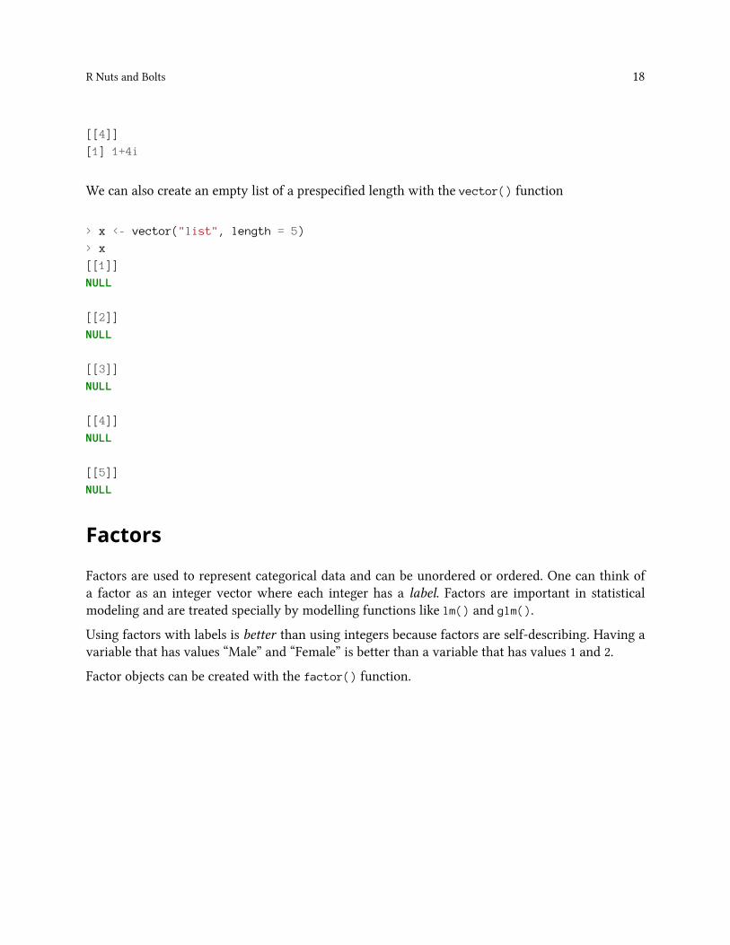
We can also create an empty list of a prespecified length with the vector() function

> x <- vector("list", length = 5)

> x

[[1]]

NULL

[[2]]

NULL

[[3]]

NULL

[[4]]

NULL

[[5]]

NULL

Factors

Factors are used to represent categorical data and can be unordered or ordered. One can think ofa factor as an integer vector where each integer has a label. Factors are important in statisticalmodeling and are treated specially by modelling functions like lm() and glm().

Using factors with labels is better than using integers because factors are self-describing. Having avariable that has values “Male” and “Female” is better than a variable that has values 1 and 2.

Factor objects can be created with the factor() function.

R Nuts and Bolts 19

> x <- factor(c("yes", "yes", "no", "yes", "no"))

> x

[1] yes yes no yes no

Levels: no yes

> table(x)

x

no yes

2 3

> ## See the underlying representation of factor

> unclass(x)

[1] 2 2 1 2 1

attr(,"levels")

[1] "no" "yes"

Often factors will be automatically created for you when you read a dataset in using a function likeread.table(). Those functions often default to creating factors when they encounter data that looklike characters or strings.

The order of the levels of a factor can be set using the levels argument to factor(). This can beimportant in linear modelling because the first level is used as the baseline level.

> x <- factor(c("yes", "yes", "no", "yes", "no"))

> x ## Levels are put in alphabetical order

[1] yes yes no yes no

Levels: no yes

> x <- factor(c("yes", "yes", "no", "yes", "no"),

+ levels = c("yes", "no"))

> x

[1] yes yes no yes no

Levels: yes no

Missing Values

Missing values are denoted by NA or NaN for q undefined mathematical operations.

• is.na() is used to test objects if they are NA• is.nan() is used to test for NaN• NA values have a class also, so there are integer NA, character NA, etc.• A NaN value is also NA but the converse is not true

R Nuts and Bolts 20

> ## Create a vector with NAs in it

> x <- c(1, 2, NA, 10, 3)

> ## Return a logical vector indicating which elements are NA

> is.na(x)

[1] FALSE FALSE TRUE FALSE FALSE

> ## Return a logical vector indicating which elements are NaN

> is.nan(x)

[1] FALSE FALSE FALSE FALSE FALSE

> ## Now create a vector with both NA and NaN values

> x <- c(1, 2, NaN, NA, 4)

> is.na(x)

[1] FALSE FALSE TRUE TRUE FALSE

> is.nan(x)

[1] FALSE FALSE TRUE FALSE FALSE

Data Frames

Data frames are used to store tabular data in R. They are an important type of object in R and areused in a variety of statistical modeling applications. Hadley Wickham’s package dplyr³⁵ has anoptimized set of functions designed to work efficiently with data frames.

Data frames are represented as a special type of list where every element of the list has to have thesame length. Each element of the list can be thought of as a column and the length of each elementof the list is the number of rows.

Unlike matrices, data frames can store different classes of objects in each column. Matrices musthave every element be the same class (e.g. all integers or all numeric).

In addition to column names, indicating the names of the variables or predictors, data frames havea special attribute called row.names which indicate information about each row of the data frame.

Data frames are usually created by reading in a dataset using the read.table() or read.csv().However, data frames can also be created explicitly with the data.frame() function or they can becoerced from other types of objects like lists.

Data frames can be converted to a matrix by calling data.matrix(). While it might seem that theas.matrix() function should be used to coerce a data frame to a matrix, almost always, what youwant is the result of data.matrix().

³⁵https://github.com/hadley/dplyr

R Nuts and Bolts 21

> x <- data.frame(foo = 1:4, bar = c(T, T, F, F))

> x

foo bar

1 1 TRUE

2 2 TRUE

3 3 FALSE

4 4 FALSE

> nrow(x)

[1] 4

> ncol(x)

[1] 2

Names

R objects can have names, which is very useful for writing readable code and self-describing objects.Here is an example of assigning names to an integer vector.

> x <- 1:3

> names(x)

NULL

> names(x) <- c("New York", "Seattle", "Los Angeles")

> x

New York Seattle Los Angeles

1 2 3

> names(x)

[1] "New York" "Seattle" "Los Angeles"

Lists can also have names, which is often very useful.

> x <- list("Los Angeles" = 1, Boston = 2, London = 3)

> x

$`Los Angeles`

[1] 1

$Boston

[1] 2

$London

[1] 3

> names(x)

[1] "Los Angeles" "Boston" "London"

Matrices can have both column and row names.

R Nuts and Bolts 22

> m <- matrix(1:4, nrow = 2, ncol = 2)

> dimnames(m) <- list(c("a", "b"), c("c", "d"))

> m

c d

a 1 3

b 2 4

Column names and row names can be set separately using the colnames() and rownames()

functions.

> colnames(m) <- c("h", "f")

> rownames(m) <- c("x", "z")

> m

h f

x 1 3

z 2 4

Note that for data frames, there is a separate function for setting the row names, the row.names()function. Also, data frames do not have column names, they just have names (like lists). So to setthe column names of a data frame just use the names() function. Yes, I know its confusing. Here’s aquick summary:

Object Set column names Set row names

data frame names() row.names()

matrix colnames() rownames()

Summary

There are a variety of different builtin-data types in R. In this chapter we have reviewed the following

• atomic classes: numeric, logical, character, integer, complex• vectors, lists• factors• missing values• data frames and matrices

All R objects can have attributes that help to describe what is in the object. Perhaps the most usefulattribute is names, such as column and row names in a data frame, or simply names in a vector orlist. Attributes like dimensions are also important as they can modify the behavior of objects, liketurning a vector into a matrix.

Getting Data In and Out of RReading and Writing Data

Watch a video of this section³⁶

There are a few principal functions reading data into R.

• read.table, read.csv, for reading tabular data• readLines, for reading lines of a text file• source, for reading in R code files (inverse of dump)• dget, for reading in R code files (inverse of dput)• load, for reading in saved workspaces• unserialize, for reading single R objects in binary form

There are of course, many R packages that have been developed to read in all kinds of other datasets,and you may need to resort to one of these packages if you are working in a specific area.

There are analogous functions for writing data to files

• write.table, for writing tabular data to text files (i.e. CSV) or connections• writeLines, for writing character data line-by-line to a file or connection• dump, for dumping a textual representation of multiple R objects• dput, for outputting a textual representation of an R object• save, for saving an arbitrary number of R objects in binary format (possibly compressed) toa file.

• serialize, for converting an R object into a binary format for outputting to a connection (orfile).

Reading Data Files with read.table()

The read.table() function is one of the most commonly used functions for reading data. The helpfile for read.table() is worth reading in its entirety if only because the function gets used a lot(run ?read.table in R). I know, I know, everyone always says to read the help file, but this one isactually worth reading.

The read.table() function has a few important arguments:

³⁶https://youtu.be/Z_dc_FADyi4

Getting Data In and Out of R 24

• file, the name of a file, or a connection• header, logical indicating if the file has a header line• sep, a string indicating how the columns are separated• colClasses, a character vector indicating the class of each column in the dataset• nrows, the number of rows in the dataset. By default read.table() reads an entire file.• comment.char, a character string indicating the comment character. This defalts to "#". If thereare no commented lines in your file, it’s worth setting this to be the empty string "".

• skip, the number of lines to skip from the beginning• stringsAsFactors, should character variables be coded as factors? This defaults to TRUE

because back in the old days, if you had data that were stored as strings, it was becausethose strings represented levels of a categorical variable. Now we have lots of data that is textdata and they don’t always represent categorical variables. So you may want to set this tobe FALSE in those cases. If you always want this to be FALSE, you can set a global option viaoptions(stringsAsFactors = FALSE). I’ve never seen so much heat generated on discussionforums about an R function argument than the stringsAsFactors argument. Seriously.

For small to moderately sized datasets, you can usually call read.table without specifying any otherarguments

> data <- read.table("foo.txt")

In this case, R will automatically

• skip lines that begin with a #• figure out how many rows there are (and how much memory needs to be allocated)• figure what type of variable is in each column of the table.

Telling R all these things directly makes R run faster and more efficiently. The read.csv() functionis identical to read.table except that some of the defaults are set differently (like the sep argument).

Reading in Larger Datasets with read.table

Watch a video of this section³⁷

With much larger datasets, there are a few things that you can do that will make your life easier andwill prevent R from choking.

• Read the help page for read.table, which contains many hints

³⁷https://youtu.be/BJYYIJO3UFI

Getting Data In and Out of R 25

• Make a rough calculation of the memory required to store your dataset (see the next sectionfor an example of how to do this). If the dataset is larger than the amount of RAM on yourcomputer, you can probably stop right here.

• Set comment.char = "" if there are no commented lines in your file.• Use the colClasses argument. Specifying this option instead of using the default can make’read.table’ run MUCH faster, often twice as fast. In order to use this option, you have to knowthe class of each column in your data frame. If all of the columns are “numeric”, for example,then you can just set colClasses = "numeric". A quick an dirty way to figure out the classesof each column is the following:

> initial <- read.table("datatable.txt", nrows = 100)

> classes <- sapply(initial, class)

> tabAll <- read.table("datatable.txt", colClasses = classes)

• Set nrows. This doesn’t make R run faster but it helps with memory usage. Amild overestimateis okay. You can use the Unix tool wc to calculate the number of lines in a file.

In general, when using R with larger datasets, it’s also useful to know a few things about yoursystem.

• How much memory is available on your system?• What other applications are in use? Can you close any of them?• Are there other users logged into the same system?• What operating system ar you using? Some operating systems can limit the amount ofmemorya single process can access

Calculating Memory Requirements for R Objects

Because R stores all of its objects physical memory, it is important to be cognizant of how muchmemory is being used up by all of the data objects residing in your workspace. One situation whereit’s particularly important to understand memory requirements is when you are reading in a newdataset into R. Fortunately, it’s easy tomake a back of the envelope calculation of howmuchmemorywill be required by a new dataset.

For example, suppose I have a data frame with 1,500,000 rows and 120 columns, all of which arenumeric data. Roughly, how much memory is required to store this data frame? Well, on mostmodern computers double precision floating point numbers³⁸ are stored using 64 bits of memory, or8 bytes. Given that information, you can do the following calculation

³⁸http://en.wikipedia.org/wiki/Double-precision_floating-point_format

Getting Data In and Out of R 26

1,500,000 × 120 × 8 bytes/numeric = 1,440,000,000 bytes= 1,440,000,000 / 220 bytes/MB= 1,373.29 MB= 1.34 GB

So the dataset would require about 1.34 GB of RAM. Most computers these days have at least thatmuch RAM. However, you need to be aware of

• what other programs might be running on your computer, using up RAM• what other R objects might already be taking up RAM in your workspace

Reading in a large dataset for which you do not have enough RAM is one easy way to freeze up yourcomputer (or at least your R session). This is usually an unpleasant experience that usually requiresyou to kill the R process, in the best case scenario, or reboot your computer, in the worst case. Somake sure to do a rough calculation of memeory requirements before reading in a large dataset.You’ll thank me later.

Using the readr PackageThe readr package is recently developed by Hadley Wickham to deal with reading in large flatfiles quickly. The package provides replacements for functions like read.table() and read.csv().The analogous functions in readr are read_table() and read_csv(). This functions are ovenmuchfaster than their base R analogues and provide a few other nice features such as progress meters.

For the most part, you can read use read_table() and read_csv() pretty much anywhere youmightuse read.table() and read.csv(). In addition, if there are non-fatal problems that occur whilereading in the data, you will get a warning and the returned data frame will have some informationabout which rows/observations triggered the warning. This can be very helpful for “debugging”problems with your data before you get neck deep in data analysis.

Using Textual and Binary Formats forStoring DataWatch a video of this chapter³⁹

There are a variety of ways that data can be stored, including structured text files like CSV or tab-delimited, or more complex binary formats. However, there is an intermediate format that is textual,but not as simple as something like CSV. The format is native to R and is somewhat readable becauseof its textual nature.

One can create a more descriptive representation of an R object by using the dput() or dump()

functions. The dump() and dput() functions are useful because the resulting textual format is edit-able, and in the case of corruption, potentially recoverable. Unlike writing out a table or CSV file,dump() and dput() preserve themetadata (sacrificing some readability), so that another user doesn’thave to specify it all over again. For example, we can preserve the class of each column of a table orthe levels of a factor variable.

Textual formats can work much better with version control programs like subversion or git whichcan only track changes meaningfully in text files. In addition, textual formats can be longer-lived;if there is corruption somewhere in the file, it can be easier to fix the problem because one can justopen the file in an editor and look at it (although this would probably only be done in a worst casescenario!). Finally, textual formats adhere to the Unix philosophy⁴⁰, if that means anything to you.

There are a few downsides to using these intermediate textual formats. The format is not very space-efficient, because all of the metadata is specified. Also, it is really only partially readable. In someinstances it might be preferable to have data stored in a CSV file and then have a separate code filethat specifies the metadata.

Using dput() and dump()

One way to pass data around is by deparsing the R object with dput() and reading it back in (parsingit) using dget().

³⁹https://youtu.be/5mIPigbNDfk⁴⁰http://www.catb.org/esr/writings/taoup/

Using Textual and Binary Formats for Storing Data 29

> ## Create a data frame

> y <- data.frame(a = 1, b = "a")

> ## Print 'dput' output to console

> dput(y)

structure(list(a = 1, b = structure(1L, .Label = "a", class = "factor")), .Names\

= c("a",

"b"), row.names = c(NA, -1L), class = "data.frame")

Notice that the dput() output is in the form of R code and that it preserves metadata like the classof the object, the row names, and the column names.

The output of dput() can also be saved directly to a file.

> ## Send 'dput' output to a file

> dput(y, file = "y.R")

> ## Read in 'dput' output from a file

> new.y <- dget("y.R")

> new.y

a b

1 1 a

Multiple objects can be deparsed at once using the dump function and read back in using source.

> x <- "foo"

> y <- data.frame(a = 1L, b = "a")

We can dump() R objects to a file by passing a character vector of their names.

> dump(c("x", "y"), file = "data.R")

> rm(x, y)

The inverse of dump() is source().

> source("data.R")

> str(y)

'data.frame': 1 obs. of 2 variables:

$ a: int 1

$ b: Factor w/ 1 level "a": 1

> x

[1] "foo"

Using Textual and Binary Formats for Storing Data 30

Binary Formats

The complement to the textual format is the binary format, which is sometimes necessary to usefor efficiency purposes, or because there’s just no useful way to represent data in a textual manner.Also, with numeric data, one can often lose precision when converting to and from a textual format,so it’s better to stick with a binary format.

The key functions for converting R objects into a binary format are save(), save.image(), andserialize(). Individual R objects can be saved to a file using the save() function.

> a <- data.frame(x = rnorm(100), y = runif(100))

> b <- c(3, 4.4, 1 / 3)

>

> ## Save 'a' and 'b' to a file

> save(a, b, file = "mydata.rda")

>

> ## Load 'a' and 'b' into your workspace

> load("mydata.rda")

If you have a lot of objects that you want to save to a file, you can save all objects in your workspaceusing the save.image() function.

> ## Save everything to a file

> save.image(file = "mydata.RData")

>

> ## load all objects in this file

> load("mydata.RData")

Notice that I’ve used the .rda extension when using save() and the .RData extension when usingsave.image(). This is just my personal preference; you can use whatever file extension you want.The save() and save.image() functions do not care. However, .rda and .RData are fairly commonextensions and you may want to use them because they are recognized by other software.

The serialize() function is used to convert individual R objects into a binary format that can becommunicated across an arbitrary connection. This may get sent to a file, but it could get sent overa network or other connection.

When you call serialize() on an R object, the output will be a raw vector coded in hexadecimalformat.

Using Textual and Binary Formats for Storing Data 31

> x <- list(1, 2, 3)

> serialize(x, NULL)

[1] 58 0a 00 00 00 02 00 03 02 01 00 02 03 00 00 00 00 13 00 00 00 03 00

[24] 00 00 0e 00 00 00 01 3f f0 00 00 00 00 00 00 00 00 00 0e 00 00 00 01

[47] 40 00 00 00 00 00 00 00 00 00 00 0e 00 00 00 01 40 08 00 00 00 00 00

[70] 00

If you want, this can be sent to a file, but in that case you are better off using something like save().

The benefit of the serialize() function is that it is the only way to perfectly represent an R objectin an exportable format, without losing precision or any metadata. If that is what you need, thenserialize() is the function for you.

Interfaces to the Outside WorldWatch a video of this chapter⁴¹

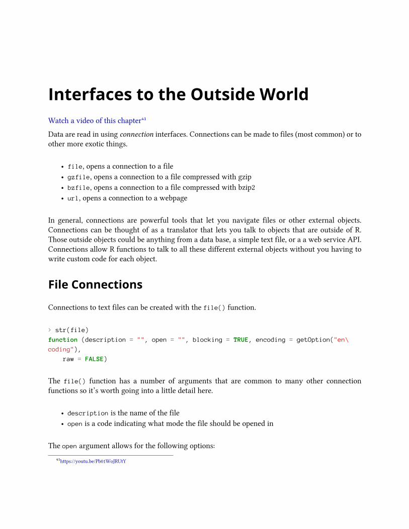
Data are read in using connection interfaces. Connections can be made to files (most common) or toother more exotic things.

• file, opens a connection to a file• gzfile, opens a connection to a file compressed with gzip• bzfile, opens a connection to a file compressed with bzip2• url, opens a connection to a webpage

In general, connections are powerful tools that let you navigate files or other external objects.Connections can be thought of as a translator that lets you talk to objects that are outside of R.Those outside objects could be anything from a data base, a simple text file, or a a web service API.Connections allow R functions to talk to all these different external objects without you having towrite custom code for each object.

File Connections

Connections to text files can be created with the file() function.

> str(file)

function (description = "", open = "", blocking = TRUE, encoding = getOption("en\

coding"),

raw = FALSE)

The file() function has a number of arguments that are common to many other connectionfunctions so it’s worth going into a little detail here.

• description is the name of the file• open is a code indicating what mode the file should be opened in

The open argument allows for the following options:

⁴¹https://youtu.be/Pb01WoJRUtY

Interfaces to the Outside World 33

• “r” open file in read only mode• “w” open a file for writing (and initializing a new file)• “a” open a file for appending• “rb”, “wb”, “ab” reading, writing, or appending in binary mode (Windows)

In practice, we often don’t need to deal with the connection interface directly as many functions forreading and writing data just deal with it in the background.

For example, if one were to explicitly use connections to read a CSV file in to R, it might look likethis,

> ## Create a connection to 'foo.txt'

> con <- file("foo.txt")

>

> ## Open connection to 'foo.txt' in read-only mode

> open(con, "r")

>

> ## Read from the connection

> data <- read.csv(con)

>

> ## Close the connection

> close(con)

which is the same as

> data <- read.csv("foo.txt")

In the background, read.csv() opens a connection to the file foo.txt, reads from it, and closes theconnection when its done.

The above example shows the basic approach to using connections. Connections must be opened,then the are read from or written to, and then they are closed.

Reading Lines of a Text File

Text files can be read line by line using the readLines() function. This function is useful for readingtext files that may be unstructured or contain non-standard data.

Interfaces to the Outside World 34

> ## Open connection to gz-compressed text file

> con <- gzfile("words.gz")

> x <- readLines(con, 10)

> x

[1] "1080" "10-point" "10th" "11-point" "12-point" "16-point"

[7] "18-point" "1st" "2" "20-point"

For more structured text data like CSV files or tab-delimited files, there are other functions likeread.csv() or read.table().

The above example used the gzfile() function which is used to create a connection to filescompressed using the gzip algorithm. This approach is useful because it allows you to read froma file without having to uncompress the file first, which would be a waste of space and time.

There is a complementary function writeLines() that takes a character vector and writes eachelement of the vector one line at a time to a text file.

Reading From a URL Connection

The readLines() function can be useful for reading in lines of webpages. Since web pages arebasically text files that are stored on a remote server, there is conceptually not much differencebetween a web page and a local text file. However, we need R to negotiate the communicationbetween your computer and the web server. This is what the url() function can do for you, bycreating a url connection to a web server.

This code might take time depending on your connection speed.

> ## Open a URL connection for reading

> con <- url("http://www.jhsph.edu", "r")

>

> ## Read the web page

> x <- readLines(con)

>

> ## Print out the first few lines

> head(x)

[1] "<!DOCTYPE html>"

[2] "<html lang=\"en\">"

[3] ""

[4] "<head>"

[5] "<meta charset=\"utf-8\" />"

[6] "<title>Johns Hopkins Bloomberg School of Public Health</title>"

Interfaces to the Outside World 35

While reading in a simple web page is sometimes useful, particularly if data are embedded in theweb page somewhere. However, more commonly we can use URL connection to read in specificdata files that are stored on web servers.

Using URL connections can be useful for producing a reproducible analysis, because the codeessentially documents where the data came from and how they were obtained. This is approachis preferable to opening a web browser and downloading a dataset by hand. Of course, the code youwrite with connections may not be executable at a later date if things on the server side are changedor reorganized.

Subsetting R ObjectsWatch a video of this section⁴²

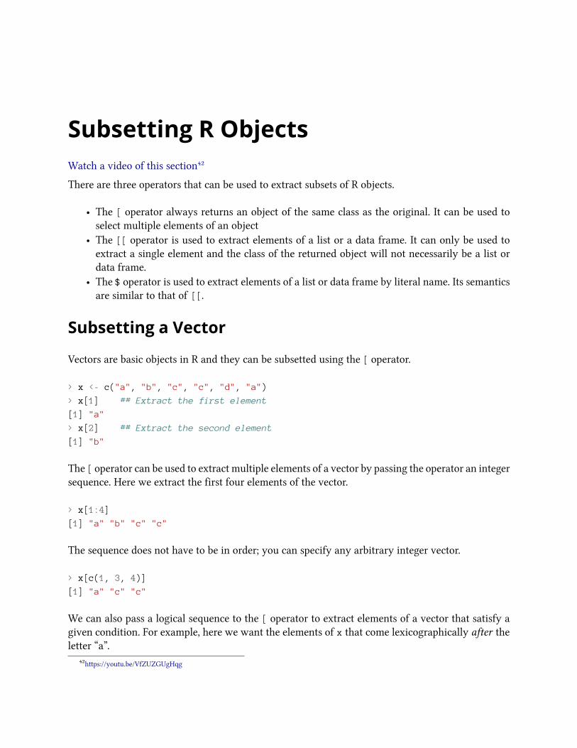
There are three operators that can be used to extract subsets of R objects.

• The [ operator always returns an object of the same class as the original. It can be used toselect multiple elements of an object

• The [[ operator is used to extract elements of a list or a data frame. It can only be used toextract a single element and the class of the returned object will not necessarily be a list ordata frame.

• The $ operator is used to extract elements of a list or data frame by literal name. Its semanticsare similar to that of [[.

Subsetting a Vector

Vectors are basic objects in R and they can be subsetted using the [ operator.

> x <- c("a", "b", "c", "c", "d", "a")

> x[1] ## Extract the first element

[1] "a"

> x[2] ## Extract the second element

[1] "b"

The [ operator can be used to extract multiple elements of a vector by passing the operator an integersequence. Here we extract the first four elements of the vector.

> x[1:4]

[1] "a" "b" "c" "c"

The sequence does not have to be in order; you can specify any arbitrary integer vector.

> x[c(1, 3, 4)]

[1] "a" "c" "c"

We can also pass a logical sequence to the [ operator to extract elements of a vector that satisfy agiven condition. For example, here we want the elements of x that come lexicographically after theletter “a”.

⁴²https://youtu.be/VfZUZGUgHqg

Subsetting R Objects 37

> u <- x > "a"

> u

[1] FALSE TRUE TRUE TRUE TRUE FALSE

> x[u]

[1] "b" "c" "c" "d"

Another, more compact, way to do this would be to skip the creation of a logical vector and justsubset the vector directly with the logical expression.

> x[x > "a"]

[1] "b" "c" "c" "d"

Subsetting a Matrix

Watch a video of this section⁴³

Matrices can be subsetted in the usual way with (i,j) type indices. Here, we create simple $2\times3$ matrix with the matrix function.

> x <- matrix(1:6, 2, 3)

> x

[,1] [,2] [,3]

[1,] 1 3 5

[2,] 2 4 6

We cna access the $(1, 2)$ or the $(2, 1)$ element of this matrix using the appropriate indices.

> x[1, 2]

[1] 3

> x[2, 1]

[1] 2

Indices can also be missing. This behavior is used to access entire rows or columns of a matrix.

> x[1, ] ## Extract the first row

[1] 1 3 5

> x[, 2] ## Extract the second column

[1] 3 4

Dropping matrix dimensions

By default, when a single element of a matrix is retrieved, it is returned as a vector of length 1 ratherthan a $1\times 1$ matrix. Often, this is exactly what we want, but this behavior can be turned offby setting drop = FALSE.

⁴³https://youtu.be/FzjXesh9tRw

Subsetting R Objects 38

> x <- matrix(1:6, 2, 3)

> x[1, 2]

[1] 3

> x[1, 2, drop = FALSE]

[,1]

[1,] 3

Similarly, when we extract a single row or column of a matrix, R by default drops the dimension oflength 1, so instead of getting a $1\times 3$ matrix after extracting the first row, we get a vector oflength 3. This behavior can similarly be turned off with the drop = FALSE option.

> x <- matrix(1:6, 2, 3)

> x[1, ]

[1] 1 3 5

> x[1, , drop = FALSE]

[,1] [,2] [,3]

[1,] 1 3 5

Be careful of R’s automatic dropping of dimensions. This is a feature that is often quite usefulduring interactive work, but can later come back to bite you when you are writing longer programsor functions.

Subsetting Lists

Watch a video of this section⁴⁴

Lists in R can be subsetted using all three of the operators mentioned above, and all three are usedfor different purposes.

> x <- list(foo = 1:4, bar = 0.6)

> x

$foo

[1] 1 2 3 4

$bar

[1] 0.6

The [[ operator can be used to extract single elements from a list. Here we extract the first elementof the list.

⁴⁴https://youtu.be/DStKguVpuDI

Subsetting R Objects 39

> x[[1]]

[1] 1 2 3 4

The [[ operator can also use named indices so that you don’t have to remember the exact orderingof every element of the list. You can also use the $ operator to extract elements by name.

> x[["bar"]]

[1] 0.6

> x$bar

[1] 0.6

Notice you don’t need the quotes when you use the $ operator.

One thing that differentiates the [[ operator from the $ is that the [[ operator can be used withcomputed indices. The $ operator can only be used with literal names.

> x <- list(foo = 1:4, bar = 0.6, baz = "hello")

> name <- "foo"

>

> ## computed index for "foo"

> x[[name]]

[1] 1 2 3 4

>

> ## element "name" doesn’t exist! (but no error here)

> x$name

NULL

>

> ## element "foo" does exist

> x$foo

[1] 1 2 3 4

Subsetting Nested Elements of a List

The [[ operator can take an integer sequence if you want to extract a nested element of a list.

Subsetting R Objects 40

> x <- list(a = list(10, 12, 14), b = c(3.14, 2.81))

>

> ## Get the 3rd element of the 1st element

> x[[c(1, 3)]]

[1] 14

>

> ## Same as above

> x[[1]][[3]]

[1] 14

>

> ## 1st element of the 2nd element

> x[[c(2, 1)]]

[1] 3.14

Extracting Multiple Elements of a List

The [ operator can be used to extract multiple elements from a list. For example, if you wanted toextract the first and third elements of a list, you would do the following

> x <- list(foo = 1:4, bar = 0.6, baz = "hello")

> x[c(1, 3)]

$foo

[1] 1 2 3 4

$baz

[1] "hello"

Note that x[c(1, 3)] is NOT the same as x[[c(1, 3)]].

Remember that the [ operator always returns an object of the same class as the original. Since theoriginal object was a list, the [ operator returns a list. In the above code, we returned a list with twoelements (the first and the third).

Partial Matching

Watch a video of this section⁴⁵

Partial matching of names is allowed with [[ and $. This is often very useful during interactive workif the object you’re working with has very long element names. You can just abbreviate those namesand R will figure out what element you’re referring to.

⁴⁵https://youtu.be/q3BNhHHVCu4

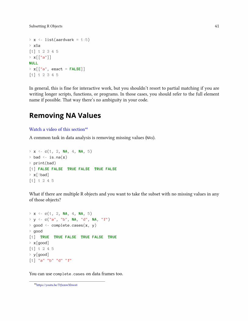
Subsetting R Objects 41

> x <- list(aardvark = 1:5)

> x$a

[1] 1 2 3 4 5

> x[["a"]]

NULL

> x[["a", exact = FALSE]]

[1] 1 2 3 4 5

In general, this is fine for interactive work, but you shouldn’t resort to partial matching if you arewriting longer scripts, functions, or programs. In those cases, you should refer to the full elementname if possible. That way there’s no ambiguity in your code.

Removing NA Values

Watch a video of this section⁴⁶

A common task in data analysis is removing missing values (NAs).

> x <- c(1, 2, NA, 4, NA, 5)

> bad <- is.na(x)

> print(bad)

[1] FALSE FALSE TRUE FALSE TRUE FALSE

> x[!bad]

[1] 1 2 4 5

What if there are multiple R objects and you want to take the subset with no missing values in anyof those objects?

> x <- c(1, 2, NA, 4, NA, 5)

> y <- c("a", "b", NA, "d", NA, "f")

> good <- complete.cases(x, y)

> good

[1] TRUE TRUE FALSE TRUE FALSE TRUE

> x[good]

[1] 1 2 4 5

> y[good]

[1] "a" "b" "d" "f"

You can use complete.cases on data frames too.

⁴⁶https://youtu.be/TtJxmwXbwo0

Subsetting R Objects 42

> head(airquality)

Ozone Solar.R Wind Temp Month Day

1 41 190 7.4 67 5 1

2 36 118 8.0 72 5 2

3 12 149 12.6 74 5 3

4 18 313 11.5 62 5 4

5 NA NA 14.3 56 5 5

6 28 NA 14.9 66 5 6

> good <- complete.cases(airquality)

> head(airquality[good, ])

Ozone Solar.R Wind Temp Month Day

1 41 190 7.4 67 5 1

2 36 118 8.0 72 5 2

3 12 149 12.6 74 5 3

4 18 313 11.5 62 5 4

7 23 299 8.6 65 5 7

8 19 99 13.8 59 5 8

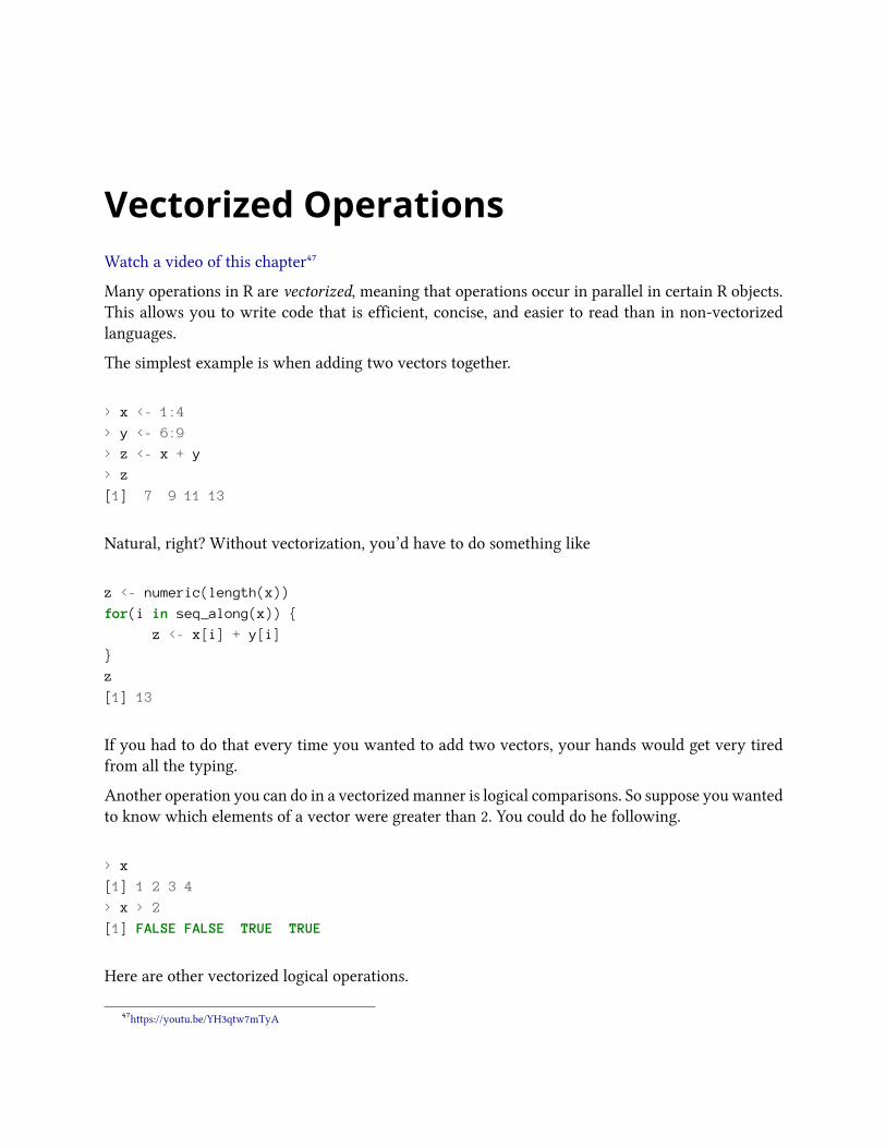
Vectorized OperationsWatch a video of this chapter⁴⁷

Many operations in R are vectorized, meaning that operations occur in parallel in certain R objects.This allows you to write code that is efficient, concise, and easier to read than in non-vectorizedlanguages.

The simplest example is when adding two vectors together.

> x <- 1:4

> y <- 6:9

> z <- x + y

> z

[1] 7 9 11 13

Natural, right? Without vectorization, you’d have to do something like

z <- numeric(length(x))

for(i in seq_along(x)) {

z <- x[i] + y[i]

}

z

[1] 13

If you had to do that every time you wanted to add two vectors, your hands would get very tiredfrom all the typing.

Another operation you can do in a vectorizedmanner is logical comparisons. So suppose you wantedto know which elements of a vector were greater than 2. You could do he following.

> x

[1] 1 2 3 4

> x > 2

[1] FALSE FALSE TRUE TRUE

Here are other vectorized logical operations.

⁴⁷https://youtu.be/YH3qtw7mTyA

Vectorized Operations 44

> x >= 2

[1] FALSE TRUE TRUE TRUE

> x < 3

[1] TRUE TRUE FALSE FALSE

> y == 8

[1] FALSE FALSE TRUE FALSE

Notice that these logical operations return a logical vector of TRUE and FALSE.

Of course, subtraction, multiplication and division are also vectorized.

> x - y

[1] -5 -5 -5 -5

> x * y

[1] 6 14 24 36

> x / y

[1] 0.1666667 0.2857143 0.3750000 0.4444444

Vectorized Matrix Operations

Matrix operations are also vectorized, making for nicly compact notation. This way, we can doelement-by-element operations on matrices without having to loop over every element.

> x <- matrix(1:4, 2, 2)

> y <- matrix(rep(10, 4), 2, 2)

>

> ## element-wise multiplication

> x * y

[,1] [,2]

[1,] 10 30

[2,] 20 40

>

> ## element-wise division

> x / y

[,1] [,2]

[1,] 0.1 0.3

[2,] 0.2 0.4

>

> ## true matrix multiplication

> x %*% y

[,1] [,2]

[1,] 40 40

[2,] 60 60

Dates and TimesR has developed a special representation for dates and times. Dates are represented by the Date classand times are represented by the POSIXct or the POSIXlt class. Dates are stored internally as thenumber of days since 1970-01-01 while times are stored internally as the number of seconds since1970-01-01.

It’s not important to know the internal representation of dates and times in order to use them in R.I just thought those were fun facts.

Dates in R

Watch a video of this section⁴⁸

Dates are represented by the Date class and can be coerced from a character string using theas.Date() function. This is a common way to end up with a Date object in R.

> ## Coerce a 'Date' object from character

> x <- as.Date("1970-01-01")

> x

[1] "1970-01-01"

You can see the internal representation of a Date object by using the unclass() function.

> unclass(x)

[1] 0

> unclass(as.Date("1970-01-02"))

[1] 1

Times in R

Watch a video of this section⁴⁹

Times are represented by the POSIXct or the POSIXlt class. POSIXct is just a very large integer underthe hood. It use a useful class when you want to store times in something like a data frame. POSIXlt

⁴⁸https://youtu.be/opYexVgjwkE⁴⁹https://youtu.be/8HENCYXwZoU

Dates and Times 46

is a list underneath and it stores a bunch of other useful information like the day of the week, dayof the year, month, day of the month. This is useful when you need that kind of information.

There are a number of generic functions that work on dates and times to help you extract pieces ofdates and/or times.

• weekdays: give the day of the week• months: give the month name• quarters: give the quarter number (“Q1”, “Q2”, “Q3”, or “Q4”)

Times can be coerced from a character string using the as.POSIXlt or as.POSIXct function.

> x <- Sys.time()

> x

[1] "2015-04-13 10:09:17 EDT"

> class(x) ## 'POSIXct' object

[1] "POSIXct" "POSIXt"

The POSIXlt object contains some useful metadata.

> p <- as.POSIXlt(x)

> names(unclass(p))

[1] "sec" "min" "hour" "mday" "mon" "year" "wday"

[8] "yday" "isdst" "zone" "gmtoff"

> p$wday ## day of the week

[1] 1

You can also use the POSIXct format.

> x <- Sys.time()

> x ## Already in ‘POSIXct’ format

[1] "2015-04-13 10:09:17 EDT"

> unclass(x) ## Internal representation

[1] 1428934157

> x$sec ## Can't do this with 'POSIXct'!

Error in x$sec: $ operator is invalid for atomic vectors

> p <- as.POSIXlt(x)

> p$sec ## That's better

[1] 17.16238

Finally, there is the strptime() function in case your dates are written in a different format.strptime() takes a character vector that has dates and times and converts them into to a POSIXltobject.

Dates and Times 47

> datestring <- c("January 10, 2012 10:40", "December 9, 2011 9:10")

> x <- strptime(datestring, "%B %d, %Y %H:%M")

> x

[1] "2012-01-10 10:40:00 EST" "2011-12-09 09:10:00 EST"

> class(x)

[1] "POSIXlt" "POSIXt"

The weird-looking symbols that start with the % symbol are the formatting strings for dates andtimes. I can never remember the formatting strings. Check ?strptime for details. It’s probably notworth memorizing this stuff.

Operations on Dates and Times

Watch a video of this section⁵⁰

You can use mathematical operations on dates and times. Well, really just + and -. You can docomparisons too (i.e. ==, <=)

> x <- as.Date("2012-01-01")

> y <- strptime("9 Jan 2011 11:34:21", "%d %b %Y %H:%M:%S")

> x-y

Warning: Incompatible methods ("-.Date", "-.POSIXt") for "-"

Error in x - y: non-numeric argument to binary operator

> x <- as.POSIXlt(x)

> x-y

Time difference of 356.3095 days

The nice thing about the date/time classes is that they keep track of all the annoying things aboutdates and times, like leap years, leap seconds, daylight savings, and time zones.

Here’s an example where a leap year gets involved.

> x <- as.Date("2012-03-01")

> y <- as.Date("2012-02-28")

> x-y

Time difference of 2 days

Here’s an example where two different time zones are in play (unless you live in GMT timezone, inwhich case they will be the same!).

⁵⁰https://youtu.be/vEmWJrpP1KM

Dates and Times 48

> ## My local time zone

> x <- as.POSIXct("2012-10-25 01:00:00")

> y <- as.POSIXct("2012-10-25 06:00:00", tz = "GMT")

> y-x

Time difference of 1 hours

Summary

• Dates and times have special classes in R that allow for numerical and statistical calculations• Dates use the Date class• Times use the POSIXct and POSIXlt class• Character strings can be coerced to Date/Time classes using the strptime function or theas.Date, as.POSIXlt, or as.POSIXct

Managing Data Frames with thedplyr packageWatch a video of this chapter⁵¹

Data Frames

The data frame is a key data structure in statistics and in R. The basic structure of a data frame isthat there is one observation per row and each column represents a variable, a measure, feature, orcharacteristic of that observation. R has an internal implementation of data frames that is likely theone you will use most often. However, there are packages on CRAN that implement data frames viathings like relational databases that allow you to operate on very very large data frames (but wewon’t discuss them here).

Given the importance of managing data frames, it’s important that we have good tools for dealingwith them. In previous chapters we have already discussed some tools like the subset() functionand the use of [ and $ operators to extract subsets of data frames. However, other operations, likefiltering, re-ordering, and collapsing, can often be tedious operations in R whose syntax is not veryintuitive. The dplyr package is designed to mitigate a lot of these problems and to provide a highlyoptimized set of routines specifically for dealing with data frames.

The dplyr Package

The dplyr package was developed by Hadley Wickham of RStudio and is an optimized and distilledversion of his plyr package. The dplyr package does not provide any “new” functionality to R per se,in the sense that everything dplyr does could already be done with base R, but it greatly simplifiesexisting functionality in R.

One important contribution of the dplyr package is that it provides a “grammar” (in particular,verbs) for data manipulation and for operating on data frames. With this grammar, you can sensiblycommunicate what it is that you are doing to a data frame that other people can understand(assuming they also know the grammar). This is useful because it provides an abstraction for datamanipulation that previously did not exist. Another useful contribution is that the dplyr functionsare very fast, as many key operations are coded in C++.

⁵¹https://youtu.be/aywFompr1F4

Managing Data Frames with the dplyr package 50

dplyr Grammar

Some of the key “verbs” provided by the dplyr package are

• select: return a subset of the columns of a data frame, using a flexible notation• filter: extract a subset of rows from a data frame based on logical conditions• arrange: reorder rows of a data frame• rename: rename variables in a data frame• mutate: add new variables/columns or transform existing variables• summarise / summarize: generate summary statistics of different variables in the data frame,possibly within strata

• %>%: the “pipe” operator is used to connect multiple verb actions together into a pipeline

The dplyr package as a number of its own data types that it takes advantage of. For example, thereis a handy print method that prevents you from printing a lot of data to the console. Most of thetime, these additional data types are transparent to the user and do not need to be worried about.

Common dplyr Function Properties

All of the functions that we will discuss in this Chapter will have a few common characteristics. Inparticular,

1. The first argument is a data frame.2. The subsequent arguments describe what to do with the data frame specified in the first

argument, and you can refer to columns in the data frame directly without using the $ operator(just use the column names).

3. The return result of a function is a new data frame4. Data frames must be properly formatted and annotated for this to all be useful. In particular,

the data must be tidy⁵². In short, there should be one observation per row, and each columnshould represent a feature or characteristic of that observation.

Installing the dplyr package

The dplyr package can be installed from CRAN or from GitHub using the devtools package andthe install_github() function. The GitHub repository will usually contain the latest updates tothe package and the development version.

To install from CRAN, just run

⁵²http://www.jstatsoft.org/v59/i10/paper

Managing Data Frames with the dplyr package 51

> install.packages("dplyr")

To install from GitHub you can run

> install_github("hadley/dplyr")

After installing the package it is important that you load it into your R session with the library()function.

> library(dplyr)

Attaching package: 'dplyr'

The following object is masked from 'package:stats':

filter

The following objects are masked from 'package:base':

intersect, setdiff, setequal, union

You may get some warnings when the package is loaded because there are functions in the dplyrpackage that have the same name as functions in other packages. For now you can ignore thewarnings.

select()

For the examples in this chapter we will be using a dataset containing air pollution and temperaturedata for the city of Chicago⁵³ in the U.S. The dataset is available from my web site.

After unzipping the archive, you can load the data into R using the readRDS() function.

> chicago <- readRDS("chicago.rds")

You can see some basic characteristics of the dataset with the dim() and str() functions.

⁵³http://www.biostat.jhsph.edu/~rpeng/leanpub/rprog/chicago_data.zip

Managing Data Frames with the dplyr package 52

> dim(chicago)

[1] 6940 8

> str(chicago)

'data.frame': 6940 obs. of 8 variables:

$ city : chr "chic" "chic" "chic" "chic" ...

$ tmpd : num 31.5 33 33 29 32 40 34.5 29 26.5 32.5 ...

$ dptp : num 31.5 29.9 27.4 28.6 28.9 ...

$ date : Date, format: "1987-01-01" "1987-01-02" ...

$ pm25tmean2: num NA NA NA NA NA NA NA NA NA NA ...

$ pm10tmean2: num 34 NA 34.2 47 NA ...

$ o3tmean2 : num 4.25 3.3 3.33 4.38 4.75 ...

$ no2tmean2 : num 20 23.2 23.8 30.4 30.3 ...

The select() function can be used to select columns of a data frame that you want to focus on.Often you’ll have a large data frame containing “all” of the data, but any given analysis might onlyuse a subset of variables or observations. The select() function allows you to get the few columnsyou might need.

Suppose we wanted to take the first 3 columns only. There are a few ways to do this. We could forexample use numerical indices. But we can also use the names directly.

> names(chicago)[1:3]

[1] "city" "tmpd" "dptp"

> subset <- select(chicago, city:dptp)

> head(subset)

city tmpd dptp

1 chic 31.5 31.500

2 chic 33.0 29.875

3 chic 33.0 27.375

4 chic 29.0 28.625

5 chic 32.0 28.875

6 chic 40.0 35.125

Note that the : normally cannot be used with names or strings, but inside the select() functionyou can use it to specify a range of variable names.

You can also omit variables using the select() function by using the negative sign. With select()

you can do

> select(chicago, -(city:dptp))

which indicates that we should include every variable except the variables city through dptp. Theequivalent code in base R would be

Managing Data Frames with the dplyr package 53

> i <- match("city", names(chicago))

> j <- match("dptp", names(chicago))

> head(chicago[, -(i:j)])

Not super intuitive, right?

The select() function also allows a special syntax that allows you to specify variable names basedon patterns. So, for example, if you wanted to keep every variable that ends with a “2”, we could do

> subset <- select(chicago, ends_with("2"))

> str(subset)

'data.frame': 6940 obs. of 4 variables:

$ pm25tmean2: num NA NA NA NA NA NA NA NA NA NA ...

$ pm10tmean2: num 34 NA 34.2 47 NA ...

$ o3tmean2 : num 4.25 3.3 3.33 4.38 4.75 ...

$ no2tmean2 : num 20 23.2 23.8 30.4 30.3 ...

Or if we wanted to keep every variable that starts with a “d”, we could do

> subset <- select(chicago, starts_with("d"))

> str(subset)

'data.frame': 6940 obs. of 2 variables:

$ dptp: num 31.5 29.9 27.4 28.6 28.9 ...

$ date: Date, format: "1987-01-01" "1987-01-02" ...

You can also use more general regular expressions if necessary. See the help page (?select) for moredetails.

filter()

The filter() function is used to extract subsets of rows from a data frame. This function is similarto the existing subset() function in R but is quite a bit faster in my experience.

Suppose we wanted to extract the rows of the chicago data frame where the levels of PM2.5 aregreater than 30 (which is a reasonably high level), we could do

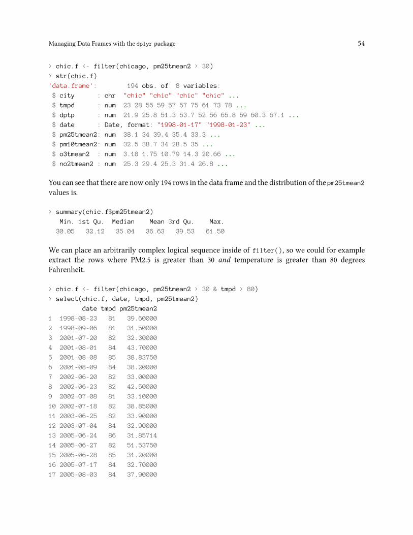
Managing Data Frames with the dplyr package 54

> chic.f <- filter(chicago, pm25tmean2 > 30)

> str(chic.f)

'data.frame': 194 obs. of 8 variables:

$ city : chr "chic" "chic" "chic" "chic" ...

$ tmpd : num 23 28 55 59 57 57 75 61 73 78 ...

$ dptp : num 21.9 25.8 51.3 53.7 52 56 65.8 59 60.3 67.1 ...

$ date : Date, format: "1998-01-17" "1998-01-23" ...

$ pm25tmean2: num 38.1 34 39.4 35.4 33.3 ...

$ pm10tmean2: num 32.5 38.7 34 28.5 35 ...

$ o3tmean2 : num 3.18 1.75 10.79 14.3 20.66 ...

$ no2tmean2 : num 25.3 29.4 25.3 31.4 26.8 ...

You can see that there are now only 194 rows in the data frame and the distribution of the pm25tmean2values is.

> summary(chic.f$pm25tmean2)

Min. 1st Qu. Median Mean 3rd Qu. Max.

30.05 32.12 35.04 36.63 39.53 61.50

We can place an arbitrarily complex logical sequence inside of filter(), so we could for exampleextract the rows where PM2.5 is greater than 30 and temperature is greater than 80 degreesFahrenheit.

> chic.f <- filter(chicago, pm25tmean2 > 30 & tmpd > 80)

> select(chic.f, date, tmpd, pm25tmean2)

date tmpd pm25tmean2

1 1998-08-23 81 39.60000

2 1998-09-06 81 31.50000

3 2001-07-20 82 32.30000

4 2001-08-01 84 43.70000

5 2001-08-08 85 38.83750

6 2001-08-09 84 38.20000

7 2002-06-20 82 33.00000

8 2002-06-23 82 42.50000

9 2002-07-08 81 33.10000

10 2002-07-18 82 38.85000

11 2003-06-25 82 33.90000

12 2003-07-04 84 32.90000

13 2005-06-24 86 31.85714

14 2005-06-27 82 51.53750

15 2005-06-28 85 31.20000

16 2005-07-17 84 32.70000

17 2005-08-03 84 37.90000

Managing Data Frames with the dplyr package 55

Now there are only 17 observations where both of those conditions are met.

arrange()

The arrange() function is used to reorder rows of a data frame according to one of the variables/-columns. Reordering rows of a data frame (while preserving corresponding order of other columns)is normally a pain to do in R. The arrange() function simplifies the process quite a bit.

Here we can order the rows of the data frame by date, so that the first row is the earliest (oldest)observation and the last row is the latest (most recent) observation.

> chicago <- arrange(chicago, date)

We can now check the first few rows

> head(select(chicago, date, pm25tmean2), 3)

date pm25tmean2

1 1987-01-01 NA

2 1987-01-02 NA

3 1987-01-03 NA

and the last few rows.

> tail(select(chicago, date, pm25tmean2), 3)

date pm25tmean2

6938 2005-12-29 7.45000

6939 2005-12-30 15.05714

6940 2005-12-31 15.00000

Columns can be arranged in descending order too by useing the special desc() operator.

> chicago <- arrange(chicago, desc(date))

Looking at the first three and last three rows shows the dates in descending order.

Managing Data Frames with the dplyr package 56

> head(select(chicago, date, pm25tmean2), 3)

date pm25tmean2

1 2005-12-31 15.00000

2 2005-12-30 15.05714

3 2005-12-29 7.45000

> tail(select(chicago, date, pm25tmean2), 3)

date pm25tmean2

6938 1987-01-03 NA

6939 1987-01-02 NA

6940 1987-01-01 NA

rename()

Renaming a variable in a data frame in R is surprisingly hard to do! The rename() function isdesigned to make this process easier.

Here you can see the names of the first five variables in the chicago data frame.

> head(chicago[, 1:5], 3)

city tmpd dptp date pm25tmean2

1 chic 35 30.1 2005-12-31 15.00000

2 chic 36 31.0 2005-12-30 15.05714

3 chic 35 29.4 2005-12-29 7.45000

The dptp column is supposed to represent the dew point temperature adn the pm25tmean2 columnprovides the PM2.5 data. However, these names are pretty obscure or awkward and probably berenamed to something more sensible.

> chicago <- rename(chicago, dewpoint = dptp, pm25 = pm25tmean2)

> head(chicago[, 1:5], 3)

city tmpd dewpoint date pm25

1 chic 35 30.1 2005-12-31 15.00000

2 chic 36 31.0 2005-12-30 15.05714

3 chic 35 29.4 2005-12-29 7.45000

The syntax inside the rename() function is to have the new name on the left-hand side of the = signand the old name on the right-hand side.

I leave it as an exercise for the reader to figure how you do this in base R without dplyr.

Managing Data Frames with the dplyr package 57

mutate()

The mutate() function exists to compute transformations of variables in a data frame. Often, youwant to create new variables that are derived from existing variables and mutate() provides a cleaninterface for doing that.

For example, with air pollution data, we often want to detrend the data by subtracting the meanfrom the data. That way we can look at whether a given day’s air pollution level is higher than orless than average (as opposed to looking at its absolute level).

Here we create a pm25detrend variable that subtracts the mean from the pm25 variable.

> chicago <- mutate(chicago, pm25detrend = pm25 - mean(pm25, na.rm = TRUE))

> head(chicago)

city tmpd dewpoint date pm25 pm10tmean2 o3tmean2 no2tmean2

1 chic 35 30.1 2005-12-31 15.00000 23.5 2.531250 13.25000

2 chic 36 31.0 2005-12-30 15.05714 19.2 3.034420 22.80556

3 chic 35 29.4 2005-12-29 7.45000 23.5 6.794837 19.97222

4 chic 37 34.5 2005-12-28 17.75000 27.5 3.260417 19.28563

5 chic 40 33.6 2005-12-27 23.56000 27.0 4.468750 23.50000

6 chic 35 29.6 2005-12-26 8.40000 8.5 14.041667 16.81944

pm25detrend

1 -1.230958

2 -1.173815

3 -8.780958

4 1.519042

5 7.329042

6 -7.830958

There is also the related transmute() function, which does the same thing as mutate() but thendrops all non-transformed variables.

Here we detrend the PM10 and ozone (O3) variables.

> head(transmute(chicago,

+ pm10detrend = pm10tmean2 - mean(pm10tmean2, na.rm = TRUE),

+ o3detrend = o3tmean2 - mean(o3tmean2, na.rm = TRUE)))

pm10detrend o3detrend

1 -10.395206 -16.904263

2 -14.695206 -16.401093

3 -10.395206 -12.640676

4 -6.395206 -16.175096

5 -6.895206 -14.966763

6 -25.395206 -5.393846

Managing Data Frames with the dplyr package 58

Note that there are only two columns in the transmuted data frame.

group_by()

The group_by() function is used to generate summary statistics from the data frame within stratadefined by a variable. For example, in this air pollution dataset, you might want to know what theaverage annual level of PM2.5 is. So the stratum is the year, and that is something we can derivefrom the date variable. In conjunction with the group_by() function we often use the summarize()function (or summarise() for some parts of the world).

The general operation here is a combination of splitting a data frame into separate pieces defined bya variable or group of variables (group_by()), and then applying a summary function across thosesubsets (summarize()).

First, we can create a year varible using as.POSIXlt().

> chicago <- mutate(chicago, year = as.POSIXlt(date)$year + 1900)

Now we can create a separate data frame that splits the original data frame by year.

> years <- group_by(chicago, year)

Finally, we compute summary statistics for each year in the data frame with the summarize()

function.

> summarize(years, pm25 = mean(pm25, na.rm = TRUE),

+ o3 = max(o3tmean2, na.rm = TRUE),

+ no2 = median(no2tmean2, na.rm = TRUE))

Source: local data frame [19 x 4]

year pm25 o3 no2

1 1987 NaN 62.96966 23.49369

2 1988 NaN 61.67708 24.52296

3 1989 NaN 59.72727 26.14062

4 1990 NaN 52.22917 22.59583

5 1991 NaN 63.10417 21.38194

6 1992 NaN 50.82870 24.78921

7 1993 NaN 44.30093 25.76993

8 1994 NaN 52.17844 28.47500

9 1995 NaN 66.58750 27.26042

10 1996 NaN 58.39583 26.38715

11 1997 NaN 56.54167 25.48143

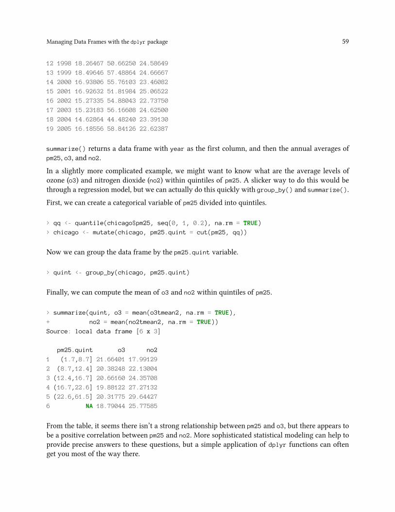
Managing Data Frames with the dplyr package 59

12 1998 18.26467 50.66250 24.58649

13 1999 18.49646 57.48864 24.66667

14 2000 16.93806 55.76103 23.46082

15 2001 16.92632 51.81984 25.06522

16 2002 15.27335 54.88043 22.73750

17 2003 15.23183 56.16608 24.62500

18 2004 14.62864 44.48240 23.39130

19 2005 16.18556 58.84126 22.62387

summarize() returns a data frame with year as the first column, and then the annual averages ofpm25, o3, and no2.

In a slightly more complicated example, we might want to know what are the average levels ofozone (o3) and nitrogen dioxide (no2) within quintiles of pm25. A slicker way to do this would bethrough a regression model, but we can actually do this quickly with group_by() and summarize().

First, we can create a categorical variable of pm25 divided into quintiles.

> qq <- quantile(chicago$pm25, seq(0, 1, 0.2), na.rm = TRUE)

> chicago <- mutate(chicago, pm25.quint = cut(pm25, qq))

Now we can group the data frame by the pm25.quint variable.

> quint <- group_by(chicago, pm25.quint)

Finally, we can compute the mean of o3 and no2 within quintiles of pm25.

> summarize(quint, o3 = mean(o3tmean2, na.rm = TRUE),

+ no2 = mean(no2tmean2, na.rm = TRUE))

Source: local data frame [6 x 3]

pm25.quint o3 no2

1 (1.7,8.7] 21.66401 17.99129

2 (8.7,12.4] 20.38248 22.13004

3 (12.4,16.7] 20.66160 24.35708

4 (16.7,22.6] 19.88122 27.27132

5 (22.6,61.5] 20.31775 29.64427

6 NA 18.79044 25.77585

From the table, it seems there isn’t a strong relationship between pm25 and o3, but there appears tobe a positive correlation between pm25 and no2. More sophisticated statistical modeling can help toprovide precise answers to these questions, but a simple application of dplyr functions can oftenget you most of the way there.

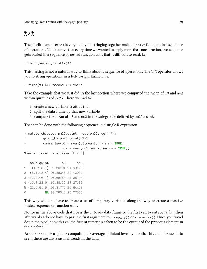
Managing Data Frames with the dplyr package 60

%>%

The pipeline operater %>% is very handy for stringing together multiple dplyr functions in a sequenceof operations. Notice above that every timewewanted to applymore than one function, the sequencegets buried in a sequence of nested function calls that is difficult to read, i.e.

> third(second(first(x)))

This nesting is not a natural way to think about a sequence of operations. The %>% operator allowsyou to string operations in a left-to-right fashion, i.e.

> first(x) %>% second %>% third

Take the example that we just did in the last section where we computed the mean of o3 and no2

within quintiles of pm25. There we had to

1. create a new variable pm25.quint2. split the data frame by that new variable3. compute the mean of o3 and no2 in the sub-groups defined by pm25.quint

That can be done with the following sequence in a single R expression.

> mutate(chicago, pm25.quint = cut(pm25, qq)) %>%

+ group_by(pm25.quint) %>%

+ summarize(o3 = mean(o3tmean2, na.rm = TRUE),

+ no2 = mean(no2tmean2, na.rm = TRUE))

Source: local data frame [6 x 3]

pm25.quint o3 no2

1 (1.7,8.7] 21.66401 17.99129

2 (8.7,12.4] 20.38248 22.13004

3 (12.4,16.7] 20.66160 24.35708

4 (16.7,22.6] 19.88122 27.27132

5 (22.6,61.5] 20.31775 29.64427

6 NA 18.79044 25.77585

This way we don’t have to create a set of temporary variables along the way or create a massivenested sequence of function calls.

Notice in the above code that I pass the chicago data frame to the first call to mutate(), but thenafterwards I do not have to pass the first argument to group_by() or summarize(). Once you traveldown the pipeline with %>%, the first argument is taken to be the output of the previous element inthe pipeline.

Another example might be computing the average pollutant level by month. This could be useful tosee if there are any seasonal trends in the data.

Managing Data Frames with the dplyr package 61

> mutate(chicago, month = as.POSIXlt(date)$mon + 1) %>%

+ group_by(month) %>%

+ summarize(pm25 = mean(pm25, na.rm = TRUE),

+ o3 = max(o3tmean2, na.rm = TRUE),

+ no2 = median(no2tmean2, na.rm = TRUE))

Source: local data frame [12 x 4]

month pm25 o3 no2

1 1 17.76996 28.22222 25.35417

2 2 20.37513 37.37500 26.78034

3 3 17.40818 39.05000 26.76984

4 4 13.85879 47.94907 25.03125

5 5 14.07420 52.75000 24.22222

6 6 15.86461 66.58750 25.01140

7 7 16.57087 59.54167 22.38442

8 8 16.93380 53.96701 22.98333

9 9 15.91279 57.48864 24.47917

10 10 14.23557 47.09275 24.15217

11 11 15.15794 29.45833 23.56537

12 12 17.52221 27.70833 24.45773

Here we can see that o3 tends to be low in the winter months and high in the summer while no2 ishigher in the winter and lower in the summer.

Summary

The dplyr package provides a concise set of operations for managing data frames. With thesefunctions we can do a number of complex operations in just a few lines of code. In particular,we can often conduct the beginnings of an exploratory analysis with the powerful combination ofgroup_by() and summarize().

Once you learn the dplyr grammar there are a few additional benefits

• dplyr can work with other data frame “backends” such as SQL databases. There is an SQLinterface for relational databases via the DBI package

• dplyr can be integrated with the data.table package for large fast tables

The dplyr package is handy way to both simplify and speed up your data frame management code.It’s rare that you get such a combination at the same time!

Control StructuresWatch a video of this section⁵⁴

Control structures in R allow you to control the flow of execution of a series of R expressions.Basically, control structures allow you to put some “logic” into your R code, rather than just alwaysexecuting the same R code every time. Control structures allow you to respond to inputs or to featuresof the data and execute different R expressions accordingly.

Commonly used control structures are

• if and else: testing a condition and acting on it• for: execute a loop a fixed number of times• while: execute a loop while a condition is true• repeat: execute an infinite loop (must break out of it to stop)• break: break the execution of a loop• next: skip an interation of a loop

Most control structures are not used in interactive sessions, but rather when writing functions orlonger expresisons. However, these constructs do not have to be used in functions and it’s a goodidea to become familiar with them before we delve into functions.

if-else

Watch a video of this section⁵⁵

The if-else combination is probably the most commonly used control structure in R (or perhapsany language). This structure allows you to test a condition and act on it depending on whether it’strue or false.

For starters, you can just use the if statement.

⁵⁴https://youtu.be/BPNLjUDZ8_o⁵⁵https://youtu.be/ZaBtJPYYGwg

Control Structures 63

if(<condition>) {

## do something

}

## Continue with rest of code

The above code does nothing if the condition is false. If you have an action you want to executewhen the condition is false, then you need an else clause.

if(<condition>) {

## do something

}

else {

## do something else

}

You can have a series of tests by following the initial if with any number of else ifs.

if(<condition1>) {

## do something

} else if(<condition2>) {

## do something different

} else {

## do something different

}

Here is an example of a valid if/else structure.

## Generate a uniform random number

x <- runif(1, 0, 10)

if(x > 3) {

y <- 10

} else {

y <- 0

}

The value of y is set depending on whether x > 3 or not. This expression can also be written adifferent, but equivalent, way in R.

Control Structures 64

y <- if(x > 3) {

10

} else {

0

}

Neither way of writing this expression is more correct than the other.Which one you use will dependon your preference and perhaps those of the team you may be working with.

Of course, the else clause is not necessary. You could have a series of if clauses that always getexecuted if their respective conditions are true.

if(<condition1>) {

}

if(<condition2>) {

}

for Loops

Watch a video of this section⁵⁶

For loops are pretty much the only looping construct that you will need in R. While you mayoccasionally find a need for other types of loops, in my experience doing data analysis, I’ve foundvery few situations where a for loop wasn’t sufficient.

In R, for loops take an interator variable and assign it successive values from a sequence or vector.For loops are most commonly used for iterating over the elements of an object (list, vector, etc.)

> for(i in 1:10) {

+ print(i)

+ }

[1] 1

[1] 2

[1] 3

[1] 4

[1] 5

[1] 6

[1] 7

⁵⁶https://youtu.be/FbT1dGXCCxU

Control Structures 65

[1] 8

[1] 9

[1] 10

This loop takes the i variable and in each iteration of the loop gives it values 1, 2, 3, …, 10, executesthe code within the curly braces, and then the loop exits.

The following three loops all have the same behavior.

> x <- c("a", "b", "c", "d")

>

> for(i in 1:4) {

+ ## Print out each element of 'x'

+ print(x[i])

+ }

[1] "a"

[1] "b"

[1] "c"

[1] "d"

The seq_along() function is commonly used in conjunction with for loops in order to generate aninteger sequence based on the length of an object (in this case, the object x).

> ## Generate a sequence based on length of 'x'

> for(i in seq_along(x)) {

+ print(x[i])

+ }

[1] "a"

[1] "b"

[1] "c"

[1] "d"

It is not necessary to use an index-type variable.

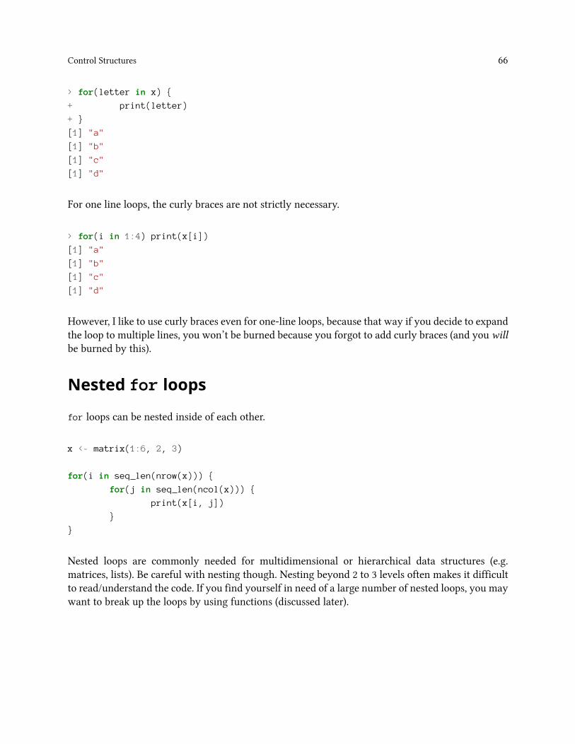
Control Structures 66

> for(letter in x) {

+ print(letter)

+ }

[1] "a"

[1] "b"

[1] "c"

[1] "d"

For one line loops, the curly braces are not strictly necessary.

> for(i in 1:4) print(x[i])

[1] "a"

[1] "b"

[1] "c"

[1] "d"

However, I like to use curly braces even for one-line loops, because that way if you decide to expandthe loop to multiple lines, you won’t be burned because you forgot to add curly braces (and youwillbe burned by this).

Nested for loops

for loops can be nested inside of each other.

x <- matrix(1:6, 2, 3)

for(i in seq_len(nrow(x))) {

for(j in seq_len(ncol(x))) {

print(x[i, j])

}

}

Nested loops are commonly needed for multidimensional or hierarchical data structures (e.g.matrices, lists). Be careful with nesting though. Nesting beyond 2 to 3 levels often makes it difficultto read/understand the code. If you find yourself in need of a large number of nested loops, you maywant to break up the loops by using functions (discussed later).

Control Structures 67

while Loops

Watch a video of this section⁵⁷

While loops begin by testing a condition. If it is true, then they execute the loop body. Once the loopbody is executed, the condition is tested again, and so forth, until the condition is false, after whichthe loop exits.

> count <- 0

> while(count < 10) {

+ print(count)

+ count <- count + 1

+ }

[1] 0

[1] 1

[1] 2

[1] 3

[1] 4

[1] 5

[1] 6

[1] 7

[1] 8

[1] 9

While loops can potentially result in infinite loops if not written properly. Use with care!

Sometimes there will be more than one condition in the test.

> z <- 5

> set.seed(1)

>

> while(z >= 3 && z <= 10) {

+ coin <- rbinom(1, 1, 0.5)

+

+ if(coin == 1) { ## random walk

+ z <- z + 1

+ } else {

+ z <- z - 1

+ }

+ }

> print(z)

[1] 2

⁵⁷https://youtu.be/VqrS1Wghq1c

Control Structures 68

Conditions are always evaluated from left to right. For example, in the above code, if z were lessthan 3, the second test would not have been evaluated.

repeat Loops

Watch a video of this section⁵⁸

repeat initiates an infinite loop right from the start. These are not commonly used in statistical ordata analysis applications but they do have their uses. The only way to exit a repeat loop is to callbreak.

One possible paradigm might be in an iterative algorith where you may be searching for a solutionand you don’t want to stop until you’re close enough to the solution. In this kind of situation, youoften don’t know in advance how many iterations it’s going to take to get “close enough” to thesolution.

x0 <- 1

tol <- 1e-8

repeat {

x1 <- computeEstimate()

if(abs(x1 - x0) < tol) { ## Close enough?

break

} else {

x0 <- x1

}

}

Note that the above code will not run if the computeEstimate() function is not defined (I just madeit up for the purposes of this demonstration).

The loop agove is a bit dangerous because there’s no guarantee it will stop. You could get in asituation where the values of x0 and x1 oscillate back and forth and never converge. Better to seta hard limit on the number of iterations by using a for loop and then report whether convergencewas achieved or not.

next, break

next is used to skip an iteration of a loop.

⁵⁸https://youtu.be/SajmdYr30SY

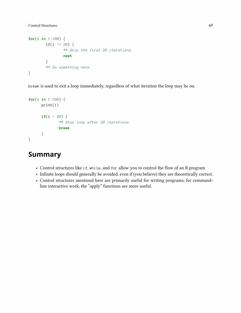
Control Structures 69

for(i in 1:100) {

if(i <= 20) {

## Skip the first 20 iterations

next

}

## Do something here

}

break is used to exit a loop immediately, regardless of what iteration the loop may be on.

for(i in 1:100) {

print(i)

if(i > 20) {

## Stop loop after 20 iterations

break

}

}

Summary

• Control structures like if, while, and for allow you to control the flow of an R program• Infinite loops should generally be avoided, even if (you believe) they are theoretically correct.• Control structures mentiond here are primarily useful for writing programs; for command-line interactive work, the “apply” functions are more useful.

FunctionsWriting functions is a core activity of an R programmer. It represents the key step of the transitionfrom a mere “user” to a developer who creates new functionality for R. Functions are often usedto encapsulate a sequence of expressions that need to be executed numerous times, perhaps underslightly different conditions. Functions are also often written when code must be shared with othersor the public.

The writing of a function allows a developer to create an interface to the code, that is explicitlyspecified with a set of parameters. This interface provides an abstraction of the code to potentialusers. This abstraction simplifies the users’ lives because it relieves them from having to know everydetail of how the code operates. In addition, the creation of an interface allows the developer tocommunicate to the user the aspects of the code that are important or are most relevant.

Functions in R

Functions in R are “first class objects”, which means that they can be treated much like any other Robject. Importantly,

• Functions can be passed as arguments to other functions. This is very handy for the variousapply funtions, like lapply() and sapply().

• Functions can be nested, so that you can define a function inside of another function

If you’re familiar with common language like C, these features might appear a bit strange. However,they are really important in R and can be useful for data analysis.

Your First Function

Functions are defined using the function() directive and are stored as R objects just like anythingelse. In particular, they are R objects of class “function”.

Here’s a simple function that takes no arguments and does nothing.

Functions 71

> f <- function() {

+ ## This is an empty function

+ }

> ## Functions have their own class

> class(f)

[1] "function"

> ## Execute this function

> f()

NULL

Not very interesting, but it’s a start. The next thing we can do is create a function that actually hasa non-trivial function body.

> f <- function() {

+ cat("Hello, world!\n")

+ }

> f()

Hello, world!

The last aspect of a basic function is the function arguments. These are the options that you canspecify to the user that the user may explicity set. For this basic function, we can add an argumentthat determines how many times “Hello, world!” is printed to the console.

> f <- function(num) {

+ for(i in seq_len(num)) {

+ cat("Hello, world!\n")

+ }

+ }

> f(3)

Hello, world!

Hello, world!

Hello, world!

Obviously, we could have just cut-and-pasted the cat("Hello, world!\n") code three times toachieve the same effect, but then we wouldn’t be programming, would we? Also, it would be un-neighborly of you to give your code to someone else and force them to cut-and-paste the codehowever many times the need to see “Hello, world!”.

In general, if you find yourself doing a lot of cutting and pasting, that’s usually a goodsign that you might need to write a function.

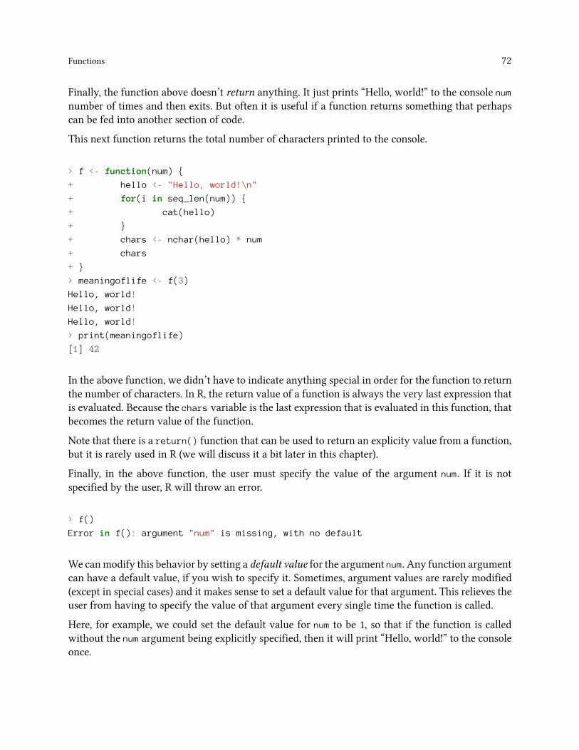
Functions 72

Finally, the function above doesn’t return anything. It just prints “Hello, world!” to the console numnumber of times and then exits. But often it is useful if a function returns something that perhapscan be fed into another section of code.

This next function returns the total number of characters printed to the console.

> f <- function(num) {

+ hello <- "Hello, world!\n"

+ for(i in seq_len(num)) {

+ cat(hello)

+ }

+ chars <- nchar(hello) * num

+ chars

+ }

> meaningoflife <- f(3)

Hello, world!

Hello, world!

Hello, world!

> print(meaningoflife)

[1] 42

In the above function, we didn’t have to indicate anything special in order for the function to returnthe number of characters. In R, the return value of a function is always the very last expression thatis evaluated. Because the chars variable is the last expression that is evaluated in this function, thatbecomes the return value of the function.

Note that there is a return() function that can be used to return an explicity value from a function,but it is rarely used in R (we will discuss it a bit later in this chapter).

Finally, in the above function, the user must specify the value of the argument num. If it is notspecified by the user, R will throw an error.

> f()

Error in f(): argument "num" is missing, with no default

We canmodify this behavior by setting a default value for the argument num. Any function argumentcan have a default value, if you wish to specify it. Sometimes, argument values are rarely modified(except in special cases) and it makes sense to set a default value for that argument. This relieves theuser from having to specify the value of that argument every single time the function is called.

Here, for example, we could set the default value for num to be 1, so that if the function is calledwithout the num argument being explicitly specified, then it will print “Hello, world!” to the consoleonce.

Functions 73

> f <- function(num = 1) {

+ hello <- "Hello, world!\n"

+ for(i in seq_len(num)) {

+ cat(hello)

+ }

+ chars <- nchar(hello) * num

+ chars

+ }

> f() ## Use default value for 'num'

Hello, world!

[1] 14

> f(2) ## Use user-specified value

Hello, world!

Hello, world!

[1] 28

Remember that the function still returns the number of characters printed to the console.

At this point, we have written a function that

• has one formal argument named num with a default value of 1. The formal arguments are thearguments included in the function definition. The formals() function returns a list of all theformal arguments of a function

• prints the message “Hello, world!” to the console a number of times indicated by the argumentnum

• returns the number of characters printed to the console

Functions have named arguments which can optionally have default values. Because all functionarguments have names, they can be specified using their name.

> f(num = 2)

Hello, world!

Hello, world!

[1] 28

Specifying an argument by its name is sometimes useful if a function hasmany arguments and it maynot always be clear which argument is being specified. Here, our function only has one argumentso there’s no confusion.

Functions 74

Argument Matching

Calling an R functionwith arguments can be done in a variety ofways. Thismay be confusing at first,but it’s really handing when doing interactive work at the command line. R functions arguments canbe matched positionally or by name. Positional matching just means that R assigns the first valueto the first argument, the second value to second argument, etc. So in the following call to rnorm()

> str(rnorm)

function (n, mean = 0, sd = 1)

> mydata <- rnorm(100, 2, 1) ## Generate some data

100 is assigned to the n argument, 2 is assigned to the mean argument, and 1 is assigned to the sd

argument, all by positional matching.

The following calls to the sd() function (which computes the empirical standard deviation of avector of numbers) are all equivalent. Note that sd() has two arguments: x indicates the vector ofnumbers and na.rm is a logical indicating whether missing values should be removed or not.

> ## Positional match first argument, default for 'na.rm'

> sd(mydata)

[1] 0.9033251

> ## Specify 'x' argument by name, default for 'na.rm'

> sd(x = mydata)

[1] 0.9033251

> ## Specify both arguments by name

> sd(x = mydata, na.rm = FALSE)

[1] 0.9033251

When specifying the function arguments by name, it doesn’t matter in what order you specify them.In the example below, we specify the na.rm argument first, followed by x, even though x is the firstargument defined in the function definition.

> ## Specify both arguments by name

> sd(na.rm = FALSE, x = mydata)

[1] 0.9033251

You can mix positional matching with matching by name. When an argument is matched by name,it is “taken out” of the argument list and the remaining unnamed arguments are matched in theorder that they are listed in the function definition.

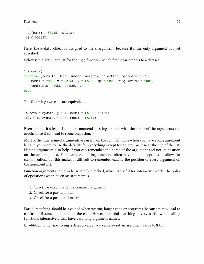
Functions 75

> sd(na.rm = FALSE, mydata)

[1] 0.9033251

Here, the mydata object is assigned to the x argument, because it’s the only argument not yetspecified.

Below is the argument list for the lm() function, which fits linear models to a dataset.

> args(lm)

function (formula, data, subset, weights, na.action, method = "qr",

model = TRUE, x = FALSE, y = FALSE, qr = TRUE, singular.ok = TRUE,

contrasts = NULL, offset, ...)

NULL

The following two calls are equivalent.

lm(data = mydata, y ~ x, model = FALSE, 1:100)

lm(y ~ x, mydata, 1:100, model = FALSE)

Even though it’s legal, I don’t recommend messing around with the order of the arguments toomuch, since it can lead to some confusion.

Most of the time, named arguments are useful on the command line when you have a long argumentlist and you want to use the defaults for everything except for an argument near the end of the list.Named arguments also help if you can remember the name of the argument and not its positionon the argument list. For example, plotting functions often have a lot of options to allow forcustomization, but this makes it difficult to remember exactly the position of every argument onthe argument list.

Function arguments can also be partially matched, which is useful for interactive work. The orderof operations when given an argument is

1. Check for exact match for a named argument2. Check for a partial match3. Check for a positional match

Partial matching should be avoided when writing longer code or programs, because it may lead toconfusion if someone is reading the code. However, partial matching is very useful when callingfunctions interactively that have very long argument names.

In addition to not specifying a default value, you can also set an argument value to NULL.

Functions 76

f <- function(a, b = 1, c = 2, d = NULL) {

}

You can check to see whether an R object is NULL with the is.null() function. It is sometimesuseful to allow an argument to take the NULL value, which might indicate that the function shouldtake some specific action.

Lazy Evaluation

Arguments to functions are evaluated lazily, so they are evaluated only as needed in the body of thefunction.

In this example, the function f() has two arguments: a and b.

> f <- function(a, b) {

+ a^2

+ }

> f(2)

[1] 4

This function never actually uses the argument b, so calling f(2) will not produce an error becausethe 2 gets positionally matched to a. This behavior can be good or bad. It’s common to write afunction that doesn’t use an argument and not notice it simply because R never throws an error.

This example also shows lazy evaluation at work, but does eventually result in an error.

> f <- function(a, b) {

+ print(a)

+ print(b)

+ }

> f(45)

[1] 45

Error in print(b): argument "b" is missing, with no default

Notice that “45” got printed first before the error was triggered. This is because b did not have tobe evaluated until after print(a). Once the function tried to evaluate print(b) the function had tothrow an error.

Functions 77

The ... Argument

There is a special argument in R known as the ... argument, which indicate a variable numberof arguments that are usually passed on to other functions. The ... argument is often used whenextending another function and you don’t want to copy the entire argument list of the originalfunction

For example, a custom plotting function may want to make use of the default plot() function alongwith its entire argument list. The function below changes the default for the type argument to thevalue type = "l" (the original default was type = "p").

myplot <- function(x, y, type = "l", ...) {

plot(x, y, type = type, ...) ## Pass '...' to 'plot' function

}

Generic functions use ... so that extra arguments can be passed to methods.

> mean

function (x, ...)

UseMethod("mean")

<bytecode: 0x7fe7bc5cf988>

<environment: namespace:base>

The ... argument is necessary when the number of arguments passed to the function cannot beknown in advance. This is clear in functions like paste() and cat().

> args(paste)

function (..., sep = " ", collapse = NULL)

NULL

> args(cat)

function (..., file = "", sep = " ", fill = FALSE, labels = NULL,

append = FALSE)

NULL

Because both paste() and cat() print out text to the console by combining multiple charactervectors together, it is impossible for those functions to know in advance howmany character vectorswill be passed to the function by the user. So the first argument to either function is ....

Arguments Coming After the ... Argument

One catch with ... is that any arguments that appear after ... on the argument list must be namedexplicitly and cannot be partially matched or matched positionally.

Take a look at the arguments to the paste() function.

Functions 78

> args(paste)

function (..., sep = " ", collapse = NULL)

NULL

With the paste() function, the arguments sep and collapse must be named explicitly and in fullif the default values are not going to be used.

Here I specify that I want “a” and “b” to be pasted together and separated by a colon.

> paste("a", "b", sep = ":")

[1] "a:b"

If I don’t specify the sep argument in full and attempt to rely on partial matching, I don’t get theexpected result.

> paste("a", "b", se = ":")

[1] "a b :"

Summary

• Functions can be defined using the function() directive and are assigned to R objects justlike any other R object

• Functions have can be defined with named arguments; these function arguments can havedefault values

• Functions arguments can be specified by name or by position in the argument list• Functions always return the last expression evaluated in the function body• A variable number of arguments can be specified using the special ... argument in a functiondefinition.

Scoping Rules of RA Diversion on Binding Values to Symbol

Watch a video of this section⁵⁹

How does R know which value to assign to which symbol? When I type

> lm <- function(x) { x * x }

> lm

function(x) { x * x }

how does R know what value to assign to the symbol lm? Why doesn’t it give it the value of lm thatis in the stats package?

When R tries to bind a value to a symbol, it searches through a series of environments to find theappropriate value. When you are working on the command line and need to retrieve the value of anR object, the order in which things occur is roughly

1. Search the global environment (i.e. your workspace) for a symbol name matching the onerequested.

2. Search the namespaces of each of the packages on the search list

The search list can be found by using the search() function.

> search()

[1] ".GlobalEnv" "package:knitr" "package:stats"

[4] "package:graphics" "package:grDevices" "package:utils"

[7] "package:datasets" "Autoloads" "package:base"

The global environment or the user’s workspace is always the first element of the search list and thebase package is always the last. For better or for worse, the order of the packages on the search listmatters, particularly if there are multiple objects with the same name in different packages.

Users can configure which packages get loaded on startup so if you are writing a function (or apackage), you cannot assume that there will be a set list of packages available in a given order.When a user loads a package with library() the namespace of that package gets put in position 2of the search list (by default) and everything else gets shifted down the list.

Note that R has separate namespaces for functions and non-functions so it’s possible to have anobject named c and a function named c().

⁵⁹https://youtu.be/ujdm01Vsrmo

Scoping Rules of R 80

Scoping Rules

The scoping rules for R are the main feature that make it different from the original S language(in case you care about that). This may seem like an esoteric aspect of R, but it’s one of its moreinteresting and useful features.

The scoping rules of a language determine how a value is associatedwith a free variable in a function.R uses lexical scoping⁶⁰ or static scoping. An alternative to lexical scoping is dynamic scoping whichis implemented by some languages. Lexical scoping turns out to be particularly useful for simplifyingstatistical computations

Related to the scoping rules is how R uses the search list to bind a value to a symbol

Consider the following function.

> f <- function(x, y) {

+ x^2 + y / z

+ }

This function has 2 formal arguments x and y. In the body of the function there is another symbolz. In this case z is called a free variable.

The scoping rules of a language determine how values are assigned to free variables. Free variablesare not formal arguments and are not local variables (assigned insided the function body).

Lexical scoping in R means that

the values of free variables are searched for in the environment in which the functionwas defined.

Okay then, what is an environment?

An environment is a collection of (symbol, value) pairs, i.e. x is a symbol and 3.14might be its value.Every environment has a parent environment and it is possible for an environment to have multiple“children”. The only environment without a parent is the empty environment.

A function, together with an environment, makes up what is called a closure or function closure.Most of the time we don’t need to think too much about a function and its associated environment(making up the closure), but occasionally, this setup can be very useful. The function closure modelcan be used to create functions that “carry around” data with them.

How do we associate a value to a free variable? There is a search process that occurs that goes asfollows:

⁶⁰http://en.wikipedia.org/wiki/Scope_(computer_science)#Lexical_scope_vs._dynamic_scope

Scoping Rules of R 81

• If the value of a symbol is not found in the environment in which a function was defined,then the search is continued in the parent environment.

• The search continues down the sequence of parent environments until we hit the top-levelenvironment ; this usually the global environment (workspace) or the namespace of a package.

• After the top-level environment, the search continues down the search list until we hit theempty environment.

If a value for a given symbol cannot be found once the empty environment is arrived at, then anerror is thrown.

One implication of this search process is that it can be affected by the number of packages you haveattached to the search list. The more packages you have attached, the more symbols R has to sortthrough in order to assign a value. That said, you’d have to have a pretty large number of packagesattached in order to notice a real difference in performance.

Lexical Scoping: Why Does It Matter?

Watch a video of this section⁶¹

Typically, a function is defined in the global environment, so that the values of free variables arejust found in the user’s workspace. This behavior is logical for most people and is usually the “rightthing” to do. However, in R you can have functions defined inside other functions (languages like Cdon’t let you do this). Now things get interesting—in this case the environment in which a functionis defined is the body of another function!

Here is an example of a function that returns another function as its return value. Remember, in Rfunctions are treated like any other object and so this is perfectly valid.

> make.power <- function(n) {

+ pow <- function(x) {

+ x^n

+ }

+ pow

+ }

The make.power() function is a kind of “constructor function” that can be used to construct otherfunctions.

⁶¹https://youtu.be/yYzPhtF6--A

Scoping Rules of R 82

> cube <- make.power(3)

> square <- make.power(2)

> cube(3)

[1] 27

> square(3)

[1] 9

Let’s take a look at the cube() function’s code.

> cube

function(x) {

x^n

}

<environment: 0x7fb01c174350>

Notice that cube() has a free variable n. What is the value of n here? Well, its value is taken fromthe environment where the function was defined. When I defined the cube() function it was whenI called make.power(3), so the value of n at that time was 3.

We can explore the environment of a function to see what objects are there and their values.

> ls(environment(cube))

[1] "n" "pow"

> get("n", environment(cube))

[1] 3

We can also take a look at the square() function.

> ls(environment(square))

[1] "n" "pow"

> get("n", environment(square))

[1] 2

Lexical vs. Dynamic Scoping

We can use the following example to demonstrate the difference between lexical and dynamicscoping rules.

Scoping Rules of R 83

> y <- 10

>

> f <- function(x) {

+ y <- 2

+ y^2 + g(x)

+ }

>

> g <- function(x) {

+ x*y

+ }

What is the value of the following expression?

f(3)

With lexical scoping the value of y in the function g is looked up in the environment in which thefunction was defined, in this case the global environment, so the value of y is 10. With dynamicscoping, the value of y is looked up in the environment from which the function was called(sometimes referred to as the calling environment). In R the calling environment is known as theparent frame. In this case, the value of y would be 2.

When a function is defined in the global environment and is subsequently called from the globalenvironment, then the defining environment and the calling environment are the same. This cansometimes give the appearance of dynamic scoping.

Consider this example.

> g <- function(x) {

+ a <- 3

+ x+a+y

+ ## 'y' is a free variable

+ }

> g(2)

Error in g(2): object 'y' not found

> y <- 3

> g(2)

[1] 8

Here, y is defined in the global environment, which also happens to be where the function g() isdefined.

There are numerous other languages that support lexical scoping, including

• Scheme

Scoping Rules of R 84

• Perl• Python• Common Lisp (all languages converge to Lisp, right?)

Lexical scoping in R has consequences beyond how free variables are looked up. In particular, it’sthe reason that all objects must be stored in memory in R. This is because all functions must carrya pointer to their respective defining environments, which could be anywhere. In the S language(R’s close cousin), free variables are always looked up in the global workspace, so everything can bestored on the disk because the “defining environment” of all functions is the same.

Application: Optimization

Watch a video of this section⁶²

NOTE: This section requires some knowledge of statistical inference and modeling. If you do nothave such knowledge, feel free to skip this section.

Why is any of this information about lexical scoping useful?

Optimization routines in R like optim(), nlm(), and optimize() require you to pass a functionwhoseargument is a vector of parameters (e.g. a log-likelihood, or a cost function). However, an objectivefunction that needst to be minimized might depend on a host of other things besides its parameters(like data). When writing software which does optimization, it may also be desirable to allow theuser to hold certain parameters fixed. The scoping rules of R allow you to abstract away much ofthe complexity involved in these kinds of problems.

Here is an example of a “constructor” function that creates a negative log-likelihood function thatcan be minimized to find maximum likelihood estimates in a statistical model.

> make.NegLogLik <- function(data, fixed = c(FALSE, FALSE)) {

+ params <- fixed

+ function(p) {

+ params[!fixed] <- p

+ mu <- params[1]

+ sigma <- params[2]

+

+ ## Calculate the Normal density

+ a <- -0.5*length(data)*log(2*pi*sigma^2)

+ b <- -0.5*sum((data-mu)^2) / (sigma^2)

+ -(a + b)

+ }

+ }

⁶²https://youtu.be/GCNZrffYLFI

Scoping Rules of R 85

Note: Optimization functions in R minimize functions, so you need to use the negative log-likelihood.

Now w ecan generate some data and then construct our negative log-likelihood.

> set.seed(1)

> normals <- rnorm(100, 1, 2)

> nLL <- make.NegLogLik(normals)

> nLL

function(p) {

params[!fixed] <- p

mu <- params[1]

sigma <- params[2]

## Calculate the Normal density

a <- -0.5*length(data)*log(2*pi*sigma^2)

b <- -0.5*sum((data-mu)^2) / (sigma^2)

-(a + b)

}

<environment: 0x7fb01c5aa0e0>

>

> ## What's in the function environment?

> ls(environment(nLL))

[1] "data" "fixed" "params"

Now that we have our nLL() function, we can try to minimize it with optim() to estimate theparameters.

> optim(c(mu = 0, sigma = 1), nLL)$par

mu sigma

1.218239 1.787343

You can see that the algorithm converged and obtained an estimate of mu and sigma.

We can also try to estimate one parameter while holding another parameter fixed. Here we fix sigmato be equal to 2.

> nLL <- make.NegLogLik(normals, c(FALSE, 2))

> optimize(nLL, c(-1, 3))$minimum

[1] 1.217775

Because we now have a one-dimensional problem, we can use the simpler optimize() functionrather than optim().

We can also try to estimate sigma while holding mu fixed at 1.

Scoping Rules of R 86

> nLL <- make.NegLogLik(normals, c(1, FALSE))

> optimize(nLL, c(1e-6, 10))$minimum

[1] 1.800596

Plotting the Likelihood

Another nice feature that you can take advantage of is plotting the negative log-likelihood to seehow peaked or flat it is.

Here is the function when mu is fixed.

> ## Fix 'mu' to be equalt o 1

> nLL <- make.NegLogLik(normals, c(1, FALSE))

> x <- seq(1.7, 1.9, len = 100)

>

> ## Evaluate 'nLL()' at every point in 'x'

> y <- sapply(x, nLL)

> plot(x, exp(-(y - min(y))), type = "l")

plot of chunk nLLFixMu

Here is the function when sigma is fixed.

Scoping Rules of R 87

> ## Fix 'sigma' to be equal to 2

> nLL <- make.NegLogLik(normals, c(FALSE, 2))

> x <- seq(0.5, 1.5, len = 100)

>

> ## Evaluate 'nLL()' at every point in 'x'

> y <- sapply(x, nLL)

> plot(x, exp(-(y - min(y))), type = "l")

plot of chunk nLLFixSigma

Summary

• Objective functions can be “built which contain all of the necessary data for evaluating thefunction

• No need to carry around long argument lists — useful for interactive and exploratory work.• Code can be simplified and cleaned up• Reference: Robert Gentleman and Ross Ihaka (2000). “Lexical Scope and Statistical Comput-ing,” JCGS, 9, 491–508.

Coding Standards for RWatch a video of this chapter⁶³

Coding standards are by no means universal and are often the subject of irrational flame wars onvarious language- or project-specfiic mailing lists. Nevertheless, I will just give you the standardsthat I use and the rationale behind them.

Always use text files / text editor. I think we can all agree on this one. Using text files and a texteditor is fundamental to coding. If you’re writing your code in an editor like Microsoft Word, youneed to stop. Interactive development environments like RStudio have nice text editors built in, butthere are many others out there.

Indent your code. Indenting is very important for the readability of your code. Some programminglanguages actually require it as part of their syntax, but R does not. Nevertheless, indenting is veryimportant. How much you should indent is up for debate, but I think each indent should be aminimum of 4 spaces, and ideally it should be 8 spaces.

Limit the width of your code. I like to limit the width of my text editor so that the code I writedoesn’t fly off into the wilderness on the right hand side. This limitation, along with the 8 spaceindentation, forces you to write code that is clean, readable, and naturally broken down intomodularunits. In particular, this combination limits your ability to write very long functions with manydifferent levels of nesting.

Limit the length of individual functions. If you are writing functions, it’s usually a good idea tonot let your functions run for pages and pages. Typically, purpose of a function is to execute oneactivity or idea. If your function is doing lots of things, it probably needs to be broken into multiplefunctions. My rule of thumb is that a function should not take up more than one page of your editor(of course, this depends on the size of your monitor).

⁶³http://youtu.be/MSPKE1y3cyQ

Loop FunctionsLooping on the Command Line

Writing for and while loops is useful when programming but not particularly easy when workinginteractively on the command line. Multi-line expressions with curly braces are just not that easy tosort through when working on the command line. R has some functions which implement loopingin a compact form to make your life easier.

• lapply(): Loop over a list and evaluate a function on each element• sapply(): Same as lapply but try to simplify the result• apply(): Apply a function over the margins of an array• tapply(): Apply a function over subsets of a vector• mapply(): Multivariate version of lapply

An auxiliary function split is also useful, particularly in conjunction with lapply.

lapply()

Watch a video of this section⁶⁴

The lapply() function does the following simple series of operations:

1. it loops over a list, iterating over each element in that list2. it applies a function to each element of the list (a function that you specify)3. and returns a list (the l is for “list”).

This function takes three arguments: (1) a list X; (2) a function (or the name of a function) FUN; (3)other arguments via its ... argument. If X is not a list, it will be coerced to a list using as.list().

The body of the lapply() function can be seen here.

⁶⁴https://youtu.be/E1_NlFb0E4g

Loop Functions 90

> lapply

function (X, FUN, ...)

{

FUN <- match.fun(FUN)

if (!is.vector(X) || is.object(X))

X <- as.list(X)

.Internal(lapply(X, FUN))

}

<bytecode: 0x7fa339937fc0>

<environment: namespace:base>

Note that the actual looping is done internally in C code for efficiency reasons.

It’s important to remember that lapply() always returns a list, regardless of the class of the input.

Here’s an example of applying the mean() function to all elements of a list. If the original list hasnames, the the names will be preserved in the output.

> x <- list(a = 1:5, b = rnorm(10))

> lapply(x, mean)

$a

[1] 3

$b

[1] 0.1322028

Notice that here we are passing the mean() function as an argument to the lapply() function.Functions in R can be used this way and can be passed back and forth as arguments just like anyother object. When you pass a function to another function, you do not need to include the openand closed parentheses () like you do when you are calling a function.

Here is another example of using lapply().

> x <- list(a = 1:4, b = rnorm(10), c = rnorm(20, 1), d = rnorm(100, 5))

> lapply(x, mean)

$a

[1] 2.5

$b

[1] 0.248845

$c

[1] 0.9935285

Loop Functions 91

$d

[1] 5.051388

You can use lapply() to evaluate a function multiple times each with a different argument. Below, isan example where I call the runif() function (to generate uniformly distributed random variables)four times, each time generating a different number of random numbers.

> x <- 1:4

> lapply(x, runif)

[[1]]

[1] 0.02778712

[[2]]

[1] 0.5273108 0.8803191

[[3]]

[1] 0.37306337 0.04795913 0.13862825

[[4]]

[1] 0.3214921 0.1548316 0.1322282 0.2213059

When you pass a function to lapply(), lapply() takes elements of the list and passes them as thefirst argument of the function you are applying. In the above example, the first argument of runif()is n, and so the elements of the sequence 1:4 all got passed to the n argument of runif().

Functions that you pass to lapply()may have other arguments. For example, the runif() functionhas a min and max argument too. In the example above I used the default values for min and max.How would you be able to specify different values for that in the context of lapply()?

Here is where the ... argument to lapply() comes into play. Any arguments that you place in the... argument will get passed down to the function being applied to the elements of the list.

Here, the min = 0 and max = 10 arguments are passed down to runif() every time it gets called.

Loop Functions 92

> x <- 1:4

> lapply(x, runif, min = 0, max = 10)

[[1]]

[1] 2.263808

[[2]]

[1] 1.314165 9.815635

[[3]]

[1] 3.270137 5.069395 6.814425

[[4]]

[1] 0.9916910 1.1890256 0.5043966 9.2925392

So now, instead of the random numbers being between 0 and 1 (the default), the are all between 0and 10.

The lapply() function and its friends make heavy use of anonymous functions. Anonymousfunctions are like members of Project Mayhem⁶⁵—they have no names. These are functions aregenerated “on the fly” as you are using lapply(). Once the call to lapply() is finished, the functiondisappears and does not appear in the workspace.

Here I am creating a list that contains two matrices.

> x <- list(a = matrix(1:4, 2, 2), b = matrix(1:6, 3, 2))

> x

$a

[,1] [,2]

[1,] 1 3

[2,] 2 4

$b

[,1] [,2]

[1,] 1 4

[2,] 2 5

[3,] 3 6

Suppose I wanted to extract the first column of each matrix in the list. I could write an anonymousfunction for extracting the first column of each matrix.

⁶⁵http://en.wikipedia.org/wiki/Fight_Club

Loop Functions 93

> lapply(x, function(elt) { elt[,1] })

$a

[1] 1 2

$b

[1] 1 2 3

Notice that I put the function() definition right in the call to lapply(). This is perfectly legal andacceptable. You can put an arbitrarily complicated function definition inside lapply(), but if it’sgoing to be more complicated, it’s probably a better idea to define the function separately.

For example, I could have done the following.

> f <- function(elt) {

+ elt[, 1]

+ }

> lapply(x, f)

$a

[1] 1 2

$b

[1] 1 2 3

Now the function is no longer anonymous; it’s name is f. Whether you use an anonymous functionor you define a function first depends on your context. If you think the function f is somethingyou’re going to need a lot in other parts of your code, you might want to define it separately. But ifyou’re just going to use it for this call to lapply(), then it’s probably simpler to use an anonymousfunction.

sapply()

The sapply() function behaves similarly to lapply(); the only real difference is in the return value.sapply() will try to simplify the result of lapply() if possible. Essentially, sapply() calls lapply()on its input and then applies the following algorithm:

• If the result is a list where every element is length 1, then a vector is returned• If the result is a list where every element is a vector of the same length (> 1), a matrix isreturned.

• If it can’t figure things out, a list is returned

Here’s the result of calling lapply().

Loop Functions 94

> x <- list(a = 1:4, b = rnorm(10), c = rnorm(20, 1), d = rnorm(100, 5))

> lapply(x, mean)

$a

[1] 2.5

$b

[1] -0.251483

$c

[1] 1.481246

$d

[1] 4.968715

Notice that lapply() returns a list (as usual), but that each element of the list has length 1.

Here’s the result of calling sapply() on the same list.

> sapply(x, mean)

a b c d

2.500000 -0.251483 1.481246 4.968715

Because the result of lapply() was a list where each element had length 1, sapply() collapsed theoutput into a numeric vector, which is often more useful than a list.

split()

Watch a video of this section⁶⁶

The split() function takes a vector or other objects and splits it into groups determined by a factoror list of factors.

The arguments to split() are

> str(split)

function (x, f, drop = FALSE, ...)

where

• x is a vector (or list) or data frame

⁶⁶https://youtu.be/TjwE5b0fOcs

Loop Functions 95

• f is a factor (or coerced to one) or a list of factors• drop indicates whether empty factors levels should be dropped

The combination of split() and a function like lapply() or sapply() is a common paradigm in R.The basic idea is that you can take a data structure, split it into subsets defined by another variable,and apply a function over those subsets. The results of applying tha function over the subsets arethen collated and returned as an object. This sequence of operations is sometimes referred to as“map-reduce” in other contexts.

Here we simulate some data and split it according to a factor variable.

> x <- c(rnorm(10), runif(10), rnorm(10, 1))

> f <- gl(3, 10)

> split(x, f)

$`1`

[1] 0.3981302 -0.4075286 1.3242586 -0.7012317 -0.5806143 -1.0010722

[7] -0.6681786 0.9451850 0.4337021 1.0051592

$`2`

[1] 0.34822440 0.94893818 0.64667919 0.03527777 0.59644846 0.41531800

[7] 0.07689704 0.52804888 0.96233331 0.70874005

$`3`

[1] 1.13444766 1.76559900 1.95513668 0.94943430 0.69418458

[6] 1.89367370 -0.04729815 2.97133739 0.61636789 2.65414530

A common idiom is split followed by an lapply.

> lapply(split(x, f), mean)

$`1`

[1] 0.07478098

$`2`

[1] 0.5266905

$`3`

[1] 1.458703

Splitting a Data Frame

Loop Functions 96

> library(datasets)

> head(airquality)

Ozone Solar.R Wind Temp Month Day

1 41 190 7.4 67 5 1

2 36 118 8.0 72 5 2

3 12 149 12.6 74 5 3

4 18 313 11.5 62 5 4

5 NA NA 14.3 56 5 5

6 28 NA 14.9 66 5 6

We can split the airquality data frame by the Month variable so that we have separate sub-dataframes for each month.

> s <- split(airquality, airquality$Month)

> str(s)

List of 5

$ 5:'data.frame': 31 obs. of 6 variables:

..$ Ozone : int [1:31] 41 36 12 18 NA 28 23 19 8 NA ...

..$ Solar.R: int [1:31] 190 118 149 313 NA NA 299 99 19 194 ...

..$ Wind : num [1:31] 7.4 8 12.6 11.5 14.3 14.9 8.6 13.8 20.1 8.6 ...

..$ Temp : int [1:31] 67 72 74 62 56 66 65 59 61 69 ...

..$ Month : int [1:31] 5 5 5 5 5 5 5 5 5 5 ...

..$ Day : int [1:31] 1 2 3 4 5 6 7 8 9 10 ...

$ 6:'data.frame': 30 obs. of 6 variables:

..$ Ozone : int [1:30] NA NA NA NA NA NA 29 NA 71 39 ...

..$ Solar.R: int [1:30] 286 287 242 186 220 264 127 273 291 323 ...

..$ Wind : num [1:30] 8.6 9.7 16.1 9.2 8.6 14.3 9.7 6.9 13.8 11.5 ...

..$ Temp : int [1:30] 78 74 67 84 85 79 82 87 90 87 ...

..$ Month : int [1:30] 6 6 6 6 6 6 6 6 6 6 ...

..$ Day : int [1:30] 1 2 3 4 5 6 7 8 9 10 ...

$ 7:'data.frame': 31 obs. of 6 variables:

..$ Ozone : int [1:31] 135 49 32 NA 64 40 77 97 97 85 ...

..$ Solar.R: int [1:31] 269 248 236 101 175 314 276 267 272 175 ...

..$ Wind : num [1:31] 4.1 9.2 9.2 10.9 4.6 10.9 5.1 6.3 5.7 7.4 ...

..$ Temp : int [1:31] 84 85 81 84 83 83 88 92 92 89 ...

..$ Month : int [1:31] 7 7 7 7 7 7 7 7 7 7 ...

..$ Day : int [1:31] 1 2 3 4 5 6 7 8 9 10 ...

$ 8:'data.frame': 31 obs. of 6 variables:

..$ Ozone : int [1:31] 39 9 16 78 35 66 122 89 110 NA ...

..$ Solar.R: int [1:31] 83 24 77 NA NA NA 255 229 207 222 ...

..$ Wind : num [1:31] 6.9 13.8 7.4 6.9 7.4 4.6 4 10.3 8 8.6 ...

..$ Temp : int [1:31] 81 81 82 86 85 87 89 90 90 92 ...

Loop Functions 97

..$ Month : int [1:31] 8 8 8 8 8 8 8 8 8 8 ...

..$ Day : int [1:31] 1 2 3 4 5 6 7 8 9 10 ...

$ 9:'data.frame': 30 obs. of 6 variables:

..$ Ozone : int [1:30] 96 78 73 91 47 32 20 23 21 24 ...

..$ Solar.R: int [1:30] 167 197 183 189 95 92 252 220 230 259 ...

..$ Wind : num [1:30] 6.9 5.1 2.8 4.6 7.4 15.5 10.9 10.3 10.9 9.7 ...

..$ Temp : int [1:30] 91 92 93 93 87 84 80 78 75 73 ...

..$ Month : int [1:30] 9 9 9 9 9 9 9 9 9 9 ...

..$ Day : int [1:30] 1 2 3 4 5 6 7 8 9 10 ...

Then we can take the column means for Ozone, Solar.R, and Wind for each sub-data frame.

> lapply(s, function(x) {

+ colMeans(x[, c("Ozone", "Solar.R", "Wind")])

+ })

$`5`

Ozone Solar.R Wind

NA NA 11.62258

$`6`

Ozone Solar.R Wind

NA 190.16667 10.26667

$`7`

Ozone Solar.R Wind

NA 216.483871 8.941935

$`8`

Ozone Solar.R Wind

NA NA 8.793548

$`9`

Ozone Solar.R Wind

NA 167.4333 10.1800

Using sapply() might be better here for a more readable output.

Loop Functions 98

> sapply(s, function(x) {

+ colMeans(x[, c("Ozone", "Solar.R", "Wind")])

+ })

5 6 7 8 9

Ozone NA NA NA NA NA

Solar.R NA 190.16667 216.483871 NA 167.4333

Wind 11.62258 10.26667 8.941935 8.793548 10.1800

Unfortunately, there are NAs in the data so we cannot simply take the means of those variables.However, we can tell the colMeans function to remove the NAs before computing the mean.

> sapply(s, function(x) {

+ colMeans(x[, c("Ozone", "Solar.R", "Wind")],

+ na.rm = TRUE)

+ })

5 6 7 8 9

Ozone 23.61538 29.44444 59.115385 59.961538 31.44828

Solar.R 181.29630 190.16667 216.483871 171.857143 167.43333

Wind 11.62258 10.26667 8.941935 8.793548 10.18000

Occasionally, we may want to split an R object according to levels defined in more than one variable.We can do this by creating an interaction of the variables with the interaction() function.

> x <- rnorm(10)

> f1 <- gl(2, 5)

> f2 <- gl(5, 2)

> f1

[1] 1 1 1 1 1 2 2 2 2 2

Levels: 1 2

> f2

[1] 1 1 2 2 3 3 4 4 5 5

Levels: 1 2 3 4 5

> ## Create interaction of two factors

> interaction(f1, f2)

[1] 1.1 1.1 1.2 1.2 1.3 2.3 2.4 2.4 2.5 2.5

Levels: 1.1 2.1 1.2 2.2 1.3 2.3 1.4 2.4 1.5 2.5

With multiple factors and many levels, creating an interaction can result in many levels that areempty.

Loop Functions 99

> str(split(x, list(f1, f2)))

List of 10

$ 1.1: num [1:2] 1.512 0.083

$ 2.1: num(0)

$ 1.2: num [1:2] 0.567 -1.025

$ 2.2: num(0)

$ 1.3: num 0.323

$ 2.3: num 1.04

$ 1.4: num(0)

$ 2.4: num [1:2] 0.0991 -0.4541

$ 1.5: num(0)

$ 2.5: num [1:2] -0.6558 -0.0359

Notice that there are 4 categories with no data. But we can drop empty levels when we call thesplit() function.

> str(split(x, list(f1, f2), drop = TRUE))

List of 6

$ 1.1: num [1:2] 1.512 0.083

$ 1.2: num [1:2] 0.567 -1.025

$ 1.3: num 0.323

$ 2.3: num 1.04

$ 2.4: num [1:2] 0.0991 -0.4541

$ 2.5: num [1:2] -0.6558 -0.0359

tapply

Watch a video of this section⁶⁷

tapply() is used to apply a function over subsets of a vector. It can be thought of as a combinationof split() and sapply() for vectors only. I’ve been told that the “t” in tapply() refers to “table”,but that is unconfirmed.

> str(tapply)

function (X, INDEX, FUN = NULL, ..., simplify = TRUE)

The arguments to tapply() are as follows:

• X is a vector

⁶⁷https://youtu.be/6YEPWjbk3GA

Loop Functions 100

• INDEX is a factor or a list of factors (or else they are coerced to factors)• FUN is a function to be applied• … contains other arguments to be passed FUN

• simplify, should we simplify the result?

Given a vector of numbers, one simple operation is to take group means.

> ## Simulate some data

> x <- c(rnorm(10), runif(10), rnorm(10, 1))

> ## Define some groups with a factor variable

> f <- gl(3, 10)

> f

[1] 1 1 1 1 1 1 1 1 1 1 2 2 2 2 2 2 2 2 2 2 3 3 3 3 3 3 3 3 3 3

Levels: 1 2 3

> tapply(x, f, mean)

1 2 3

0.1896235 0.5336667 0.9568236

We can also take the group means without simplifying the result, which will give us a list. Forfunctions that return a single value, usually, this is not what we want, but it can be done.

> tapply(x, f, mean, simplify = FALSE)

$`1`

[1] 0.1896235

$`2`

[1] 0.5336667

$`3`

[1] 0.9568236

We can also apply functions that return more than a single value. In this case, tapply() will notsimplify the result and will return a list. Here’s an example of finding the range of each sub-group.

Loop Functions 101

> tapply(x, f, range)

$`1`

[1] -1.869789 1.497041

$`2`

[1] 0.09515213 0.86723879

$`3`

[1] -0.5690822 2.3644349

apply()

Watch a video of this section⁶⁸

The apply() function is used to a evaluate a function (often an anonymous one) over the marginsof an array. It is most often used to apply a function to the rows or columns of a matrix (which isjust a 2-dimensional array). However, it can be used with general arrays, for example, to take theaverage of an array of matrices. Using apply() is not really faster than writing a loop, but it worksin one line and is highly compact.

> str(apply)

function (X, MARGIN, FUN, ...)

The arguments to apply() are

• X is an array• MARGIN is an integer vector indicating which margins should be “retained”.• FUN is a function to be applied• ... is for other arguments to be passed to FUN

Here I create a 20 by 10matrix of Normal random numbers. I then compute themean of each column.

> x <- matrix(rnorm(200), 20, 10)

> apply(x, 2, mean) ## Take the mean of each column

[1] 0.02218266 -0.15932850 0.09021391 0.14723035 -0.22431309

[6] -0.49657847 0.30095015 0.07703985 -0.20818099 0.06809774

I can also compute the sum of each row.

⁶⁸https://youtu.be/F54ixFPq_xQ

Loop Functions 102

> apply(x, 1, sum) ## Take the mean of each row

[1] -0.48483448 5.33222301 -3.33862932 -1.39998450 2.37859098

[6] 0.01082604 -6.29457190 -0.26287700 0.71133578 -3.38125293

[11] -4.67522818 3.01900232 -2.39466347 -2.16004389 5.33063755

[16] -2.92024635 3.52026401 -1.84880901 -4.10213912 5.30667310

Note that in both calls to apply(), the return value was a vector of numbers.

You’ve probably noticed that the second argument is either a 1 or a 2, depending on whether wewant row statistics or column statistics. What exactly is the second argument to apply()?

The MARGIN argument essentially indicates to apply() which dimension of the array you want topreserve or retain. So when taking the mean of each column, I specify

> apply(x, 2, mean)

because I want to collapse the first dimension (the rows) by taking the mean and I want to preservethe number of columns. Similarly, when I want the row sums, I run

> apply(x, 1, mean)

because I want to collapse the columns (the second dimension) and preserve the number of rows(the first dimension).

Col/Row Sums and Means

For the special case of column/row sums and column/row means of matrices, we have some usefulshortcuts.

• rowSums = apply(x, 1, sum)

• rowMeans = apply(x, 1, mean)

• colSums = apply(x, 2, sum)

• colMeans = apply(x, 2, mean)

The shortcut functions are heavily optimized and hence are much faster, but you probably won’tnotice unless you’re using a large matrix. Another nice aspect of these functions is that they are abit more descriptive. It’s arguably more clear to write colMeans(x) in your code than apply(x, 2,

mean).

Other Ways to Apply

You can do more than take sums and means with the apply() function. For example, you cancompute quantiles of the rows of a matrix using the quantile() function.

Loop Functions 103

> x <- matrix(rnorm(200), 20, 10)

> ## Get row quantiles

> apply(x, 1, quantile, probs = c(0.25, 0.75))

[,1] [,2] [,3] [,4] [,5] [,6]

25% -1.0884151 -0.6693040 0.2908481 -0.4602083 -1.0432010 -1.12773555

75% 0.1843547 0.8210295 1.3667301 0.4424153 0.3571219 0.03653687

[,7] [,8] [,9] [,10] [,11] [,12]

25% -1.4571706 -0.2406991 -0.3226845 -0.329898 -0.8677524 -0.2023664

75% -0.1705336 0.6504486 1.1460854 1.247092 0.4138139 0.9145331

[,13] [,14] [,15] [,16] [,17] [,18]

25% -0.9796050 -1.3551031 -0.1823252 -1.260911898 -0.9954289 -0.3767354

75% 0.5448777 -0.5396766 0.7795571 0.002908451 0.4323192 0.7542638

[,19] [,20]

25% -0.8557544 -0.7000363

75% 0.5440158 0.5432995

Notice that I had to pass the probs = c(0.25, 0.75) argument to quantile() via the ... argumentto apply().

For a higher dimensional example, I can create an array of $2\times 2$ matrices and the computethe average of the matrices in the array.

> a <- array(rnorm(2 * 2 * 10), c(2, 2, 10))

> apply(a, c(1, 2), mean)

[,1] [,2]

[1,] 0.1681387 -0.1039673

[2,] 0.3519741 -0.4029737

In the call to apply() here, I indicated via the MARGIN argument that I wanted to preserve the firstand second dimensions and to collapse the third dimension by taking the mean.

There is a faster way to do this specific operation via the colMeans() function.

> rowMeans(a, dims = 2) ## Faster

[,1] [,2]

[1,] 0.1681387 -0.1039673

[2,] 0.3519741 -0.4029737

In this situation, I might argue that the use of rowMeans() is less readable, but it is substantiallyfaster with large arrays.

Loop Functions 104

mapply()

Watch a video of this section⁶⁹

The mapply() function is a multivariate apply of sorts which applies a function in parallel over aset of arguments. Recall that lapply() and friends only iterate over a single R object. What if youwant to iterate over multiple R objects in parallel? This is what mapply() is for.

> str(mapply)

function (FUN, ..., MoreArgs = NULL, SIMPLIFY = TRUE, USE.NAMES = TRUE)

The arguments to mapply() are

• FUN is a function to apply• ... contains R objects to apply over• MoreArgs is a list of other arguments to FUN.• SIMPLIFY indicates whether the result should be simplified

The mapply() function has a different argument order from lapply() because the function to applycomes first rather than the object to iterate over. The R objects over which we apply the functionare given in the ... argument because we can apply over an arbitrary number of R objects.

For example, the following is tedious to type

list(rep(1, 4), rep(2, 3), rep(3, 2), rep(4, 1))

With mapply(), instead we can do

> mapply(rep, 1:4, 4:1)

[[1]]

[1] 1 1 1 1

[[2]]

[1] 2 2 2

[[3]]

[1] 3 3

[[4]]

[1] 4

This passes the sequence 1:4 to the first argument of rep() and the sequence 4:1 to the secondargument.

Here’s another example for simulating randon Normal variables.

⁶⁹https://youtu.be/z8jC_h7S0VE

Loop Functions 105

> noise <- function(n, mean, sd) {

+ rnorm(n, mean, sd)

+ }

> ## Simulate 5 randon numbers

> noise(5, 1, 2)

[1] -0.5196913 3.2979182 -0.6849525 1.7828267 2.7827545

>

> ## This only simulates 1 set of numbers, not 5

> noise(1:5, 1:5, 2)

[1] -1.670517 2.796247 2.776826 5.351488 3.422804

Here we can use mapply() to pass the sequence 1:5 separately to the noise() function so that wecan get 5 sets of random numbers, each with a different length and mean.

> mapply(noise, 1:5, 1:5, 2)

[[1]]

[1] 0.8260273

[[2]]

[1] 4.764568 2.336980

[[3]]

[1] 4.6463819 2.5582108 0.9412167

[[4]]

[1] 3.978149 1.550018 -1.192223 6.338245

[[5]]

[1] 2.826182 1.347834 6.990564 4.976276 3.800743

The above call to mapply() is the same as

> list(noise(1, 1, 2), noise(2, 2, 2),

+ noise(3, 3, 2), noise(4, 4, 2),

+ noise(5, 5, 2))

[[1]]

[1] 0.644104

[[2]]

[1] 1.148037 3.993318

[[3]]

Loop Functions 106

[1] 4.4553214 -0.4532612 3.7067970

[[4]]

[1] 5.4536273 5.3365220 -0.8486346 3.5292851

[[5]]

[1] 8.959267 6.593589 1.581448 1.672663 5.982219

Vectorizing a Function

The mapply() function can be use to automatically “vectorize” a function. What this means is that itcan be used to take a function that typically only takes single arguments and create a new functionthat can take vector arguments. This is often needed when you want to plot functions.

Here’s an example of a function that computes the sum of squares given some data, amean parameterand a standard deviation. The formula is $\sum_{i=1}n (x_i-\mu)2/\sigmaˆ2$.

> sumsq <- function(mu, sigma, x) {

+ sum(((x - mu) / sigma)^2)

+ }

This function takes a mean mu, a standard deviation sigma, and some data in a vector x.

In many statistical applications, we want to minimize the sum of squares to find the optimal mu andsigma. Before we do that, we may want to evaluate or plot the function for many different valuesof mu or sigma. However, passing a vector of mus or sigmas won’t work with this function becauseit’s not vectorized.

> x <- rnorm(100) ## Generate some data

> sumsq(1:10, 1:10, x) ## This is not what we want

[1] 110.2594

Note that the call to sumsq() only produced one value instead of 10 values.

However, we can do what we want to do by using mapply().

> mapply(sumsq, 1:10, 1:10, MoreArgs = list(x = x))

[1] 196.2289 121.4765 108.3981 104.0788 102.1975 101.2393 100.6998

[8] 100.3745 100.1685 100.0332

There’s even a function in R called Vectorize() that automatically can create a vectorized versionof your function. So we could create a vsumsq() function that is fully vectorized as follows.

Loop Functions 107

> vsumsq <- Vectorize(sumsq, c("mu", "sigma"))

> vsumsq(1:10, 1:10, x)

[1] 196.2289 121.4765 108.3981 104.0788 102.1975 101.2393 100.6998

[8] 100.3745 100.1685 100.0332

Pretty cool, right?

Summary

• The loop functions in R are very powerful because they allow you to conduct a series ofoperations on data using a compact form

• The operation of a loop function involves iterating over an R object (e.g. a list or vector ormatrix), applying a function to each element of the object, and the collating the results andreturning the collated results.

• Loop functions make heavy use of anonymous functions, which exist for the life of the loopfunction but are not stored anywhere

• The split() function can be used to divide an R object in to subsets determined by anothervariable which can subsequently be looped over using loop functions.

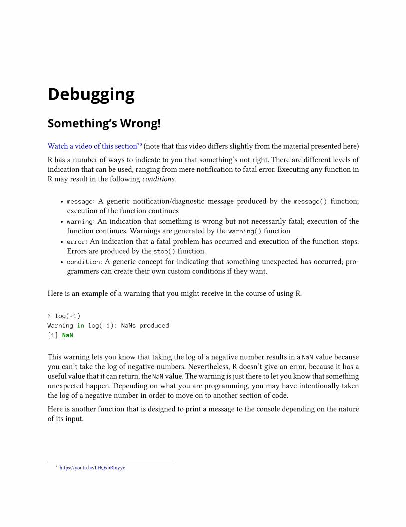
DebuggingSomething’s Wrong!

Watch a video of this section⁷⁰ (note that this video differs slightly from the material presented here)

R has a number of ways to indicate to you that something’s not right. There are different levels ofindication that can be used, ranging from mere notification to fatal error. Executing any function inR may result in the following conditions.

• message: A generic notification/diagnostic message produced by the message() function;execution of the function continues

• warning: An indication that something is wrong but not necessarily fatal; execution of thefunction continues. Warnings are generated by the warning() function

• error: An indication that a fatal problem has occurred and execution of the function stops.Errors are produced by the stop() function.

• condition: A generic concept for indicating that something unexpected has occurred; pro-grammers can create their own custom conditions if they want.

Here is an example of a warning that you might receive in the course of using R.

> log(-1)

Warning in log(-1): NaNs produced

[1] NaN

This warning lets you know that taking the log of a negative number results in a NaN value becauseyou can’t take the log of negative numbers. Nevertheless, R doesn’t give an error, because it has auseful value that it can return, the NaN value. Thewarning is just there to let you know that somethingunexpected happen. Depending on what you are programming, you may have intentionally takenthe log of a negative number in order to move on to another section of code.

Here is another function that is designed to print a message to the console depending on the natureof its input.

⁷⁰https://youtu.be/LHQxbRInyyc

Debugging 109

> printmessage <- function(x) {

+ if(x > 0)

+ print("x is greater than zero")

+ else

+ print("x is less than or equal to zero")

+ invisible(x)

+ }

This function is simple—it prints a message telling you whether x is greater than zero or less than orequal to zero. It also returns its input invisibly, which is a common practice with “print” functions.Returning an object invisibly means that the return value does not get auto-printed when thefunction is called.

Take a hard look at the function above and see if you can identify any bugs or problems.

We can execute the function as follows.

> printmessage(1)

[1] "x is greater than zero"

The function seems to work fine at this point. No errors, warnings, or messages.

> printmessage(NA)

Error in if (x > 0) print("x is greater than zero") else print("x is less than o\

r equal to zero"): missing value where TRUE/FALSE needed

What happened?

Well, the first thing the function does is test if x > 0. But you can’t do that test if x is a NA or NaNvalue. R doesn’t know what to do in this case so it stops with a fatal error.

We can fix this problem by anticipating the possibility of NA values and checking to see if the inputis NA with the is.na() function.

> printmessage2 <- function(x) {

+ if(is.na(x))

+ print("x is a missing value!")

+ else if(x > 0)

+ print("x is greater than zero")

+ else

+ print("x is less than or equal to zero")

+ invisible(x)

+ }

Now we can run the following.

Debugging 110

> printmessage2(NA)

[1] "x is a missing value!"

And all is fine.

Now what about the following situation.

> x <- log(c(-1, 2))

Warning in log(c(-1, 2)): NaNs produced

> printmessage2(x)

Warning in if (is.na(x)) print("x is a missing value!") else if (x > 0)

print("x is greater than zero") else print("x is less than or equal to

zero"): the condition has length > 1 and only the first element will be

used

[1] "x is a missing value!"

Now what?? Why are we getting this warning? The warning says “the condition has length > 1 andonly the first element will be used”.

The problem here is that I passed printmessage2() a vector x that was of length 2 rather then length1. Inside the body of printmessage2() the expression is.na(x) returns a vector that is tested in theif statement. However, if cannot take vector arguments so you get a warning. The fundamentalproblem here is that printmessage2() is not vectorized.

We can solve this problem two ways. One is by simply not allowing vector arguments. The otherway is to vectorize the printmessage2() function to allow it to take vector arguments.

For the first way, we simply need to check the length of the input.

> printmessage3 <- function(x) {

+ if(length(x) > 1L)

+ stop("'x' has length > 1")

+ if(is.na(x))

+ print("x is a missing value!")

+ else if(x > 0)

+ print("x is greater than zero")

+ else

+ print("x is less than or equal to zero")

+ invisible(x)

+ }

Now when we pass printmessage3() a vector we should get an error.

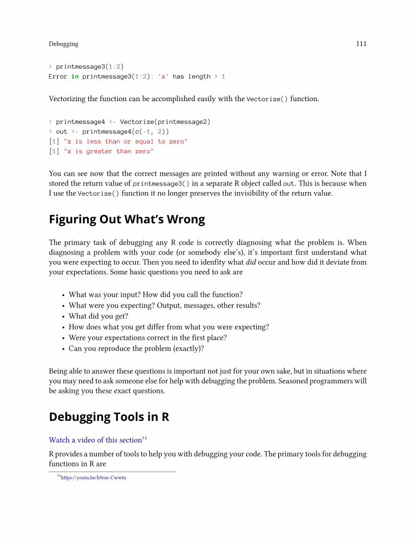
Debugging 111

> printmessage3(1:2)

Error in printmessage3(1:2): 'x' has length > 1

Vectorizing the function can be accomplished easily with the Vectorize() function.

> printmessage4 <- Vectorize(printmessage2)

> out <- printmessage4(c(-1, 2))

[1] "x is less than or equal to zero"

[1] "x is greater than zero"

You can see now that the correct messages are printed without any warning or error. Note that Istored the return value of printmessage3() in a separate R object called out. This is because whenI use the Vectorize() function it no longer preserves the invisibility of the return value.

Figuring Out What’s Wrong

The primary task of debugging any R code is correctly diagnosing what the problem is. Whendiagnosing a problem with your code (or somebody else’s), it’s important first understand whatyou were expecting to occur. Then you need to idenfity what did occur and how did it deviate fromyour expectations. Some basic questions you need to ask are

• What was your input? How did you call the function?• What were you expecting? Output, messages, other results?• What did you get?• How does what you get differ from what you were expecting?• Were your expectations correct in the first place?• Can you reproduce the problem (exactly)?

Being able to answer these questions is important not just for your own sake, but in situations whereyoumay need to ask someone else for help with debugging the problem. Seasoned programmers willbe asking you these exact questions.

Debugging Tools in R

Watch a video of this section⁷¹

R provides a number of tools to help you with debugging your code. The primary tools for debuggingfunctions in R are

⁷¹https://youtu.be/h9rs6-Cwwto

Debugging 112

• traceback(): prints out the function call stack after an error occurs; does nothing if there’sno error

• debug(): flags a function for “debug” mode which allows you to step through execution of afunction one line at a time

• browser(): suspends the execution of a function wherever it is called and puts the function indebug mode

• trace(): allows you to insert debugging code into a function a specific places• recover(): allows you to modify the error behavior so that you can browse the function callstack

These functions are interactive tools specifically designed to allow you to pick through a function.There’s also the more blunt technique of inserting print() or cat() statements in the function.

Using traceback()

Watch a video of this section⁷²

The traceback() function prints out the function call stack after an error has occurred. The functioncall stack is the sequence of functions that was called before the error occurred.

For example, youmay have a function a()which subsequently calls function b()which calls c() andthen d(). If an error occurs, it may not be immediately clear in which function the error occurred.The tracback() function shows you how many levels deep you were when the error occurred.

> mean(x)

Error in mean(x) : object 'x' not found

> traceback()

1: mean(x)

Here, it’s clear that the error occurred inside the mean() function because the object x does not exist.

The traceback() function must be called immediately after an error occurs. Once another functionis called, you lose the traceback.

Here is a slightly more complicated example using the lm() function for linear modeling.

⁷²https://youtu.be/VT9ZxCp6o-I

Debugging 113

> lm(y ~ x)

Error in eval(expr, envir, enclos) : object ’y’ not found

> traceback()

7: eval(expr, envir, enclos)

6: eval(predvars, data, env)

5: model.frame.default(formula = y ~ x, drop.unused.levels = TRUE)

4: model.frame(formula = y ~ x, drop.unused.levels = TRUE)

3: eval(expr, envir, enclos)

2: eval(mf, parent.frame())

1: lm(y ~ x)

You can see now that the error did not get thrown until the 7th level of the function call stack, inwhich case the eval() function tried to evaluate the formula y ∼ x and realized the object y didnot exist.

Looking at the traceback is useful for figuring out roughly where an error occurred but it’s not usefulfor more detailed debugging. For that you might turn to the debug() function.

Using debug()

The debug() function initiates an interactive debugger (also known as the “browser” in R) for afunction. With the debugger, you can step through an R function one expression at a time to pinpointexactly where an error occurs.

The debug() function takes a function as its first argument. Here is an example of debugging thelm() function.

> debug(lm) ## Flag the 'lm()' function for interactive debugging

> lm(y ~ x)

debugging in: lm(y ~ x)

debug: {

ret.x <- x

ret.y <- y

cl <- match.call()

...

if (!qr)

z$qr <- NULL

z

}

Browse[2]>

Now, every time you call the lm() function it will launch the interactive debugger. To turn thisbehavior off you need to call the undebug() function.

Debugging 114

The debugger calls the browser at the very top level of the function body. From there you can stepthrough each expression in the body. There are a few special commands you can call in the browser:

• n executes the current expression and moves to the next expression• c continues execution of the function and does not stop until either an error or the functionexits

• Q quits the browser

Here’s an example of a browser session with the lm() function.

Browse[2]> n ## Evalute this expression and move to the next one

debug: ret.x <- x

Browse[2]> n

debug: ret.y <- y

Browse[2]> n

debug: cl <- match.call()

Browse[2]> n

debug: mf <- match.call(expand.dots = FALSE)

Browse[2]> n

debug: m <- match(c("formula", "data", "subset", "weights", "na.action",

"offset"), names(mf), 0L)

While you are in the browser you can execute any other R function that might be available to youin a regular session. In particular, you can use ls() to see what is in your current environment (thefunction environment) and print() to print out the values of R objects in the function environment.

You can turn off interactive debugging with the undebug() function.

undebug(lm) ## Unflag the 'lm()' function for debugging

Using recover()

The recover() function can be used to modify the error behavior of R when an error occurs.Normally, when an error occurs in a function, R will print out an error message, exit out of thefunction, and return you to your workspace to await further commands.

With recover() you can tell R that when an error occurs, it should halt execution at the exact pointat which the error occurred. That can give you the opportunity to poke around in the environmentin which the error occurred. This can be useful to see if there are any R objects or data that havebeen corrupted or mistakenly modified.

Debugging 115

> options(error = recover) ## Change default R error behavior

> read.csv("nosuchfile") ## This code doesn't work

Error in file(file, "rt") : cannot open the connection

In addition: Warning message:

In file(file, "rt") :

cannot open file ’nosuchfile’: No such file or directory

Enter a frame number, or 0 to exit

1: read.csv("nosuchfile")

2: read.table(file = file, header = header, sep = sep, quote = quote, dec =

3: file(file, "rt")

Selection:

The recover() function will first print out the function call stack when an error occurrs. Then, youcan choose to jump around the call stack and investigate the problem. When you choose a framenumber, you will be put in the browser (just like the interactive debugger triggered with debug())and will have the ability to poke around.

Summary

• There are three main indications of a problem/condition: message, warning, error; only anerror is fatal

• When analyzing a function with a problem, make sure you can reproduce the problem, clearlystate your expectations and how the output differs from your expectation

• Interactive debugging tools traceback, debug, browser, trace, and recover can be used tofind problematic code in functions

• Debugging tools are not a substitute for thinking!

Profiling R CodeLet’s solve the problem but let’s not make it worse by guessing. —Gene Kranz, Apollo13 Lead Flight Director

Watch a video of this section⁷³

R comes with a profiler to help you optimize your code and improve its performance. In generall, it’susually a bad idea to focus on optimizing your code at the very beginning of development. Rather, inthe beginning it’s better to focus on translating your ideas into code and writing code that’s coherentand readable. The problem is that heavily optimized code tends to be obscure and difficult to read,making it harder to debug and revise. Better to get all the bugs out first, then focus on optimizing.

Of course, when it comes to optimizing code, the question is what should you optimize?Well, clearlyshould optimize the parts of your code that are running slowly, but how do we know what partsthose are?

This is what the profiler is for. Profiling is a systematic way to examine how much time is spent indifferent parts of a program.

Sometimes profiling becomes necessary as a project grows and layers of code are placed on top ofeach other. Often you might write some code that runs fine once. But then later, you might put thatsame code in a big loop that runs 1,000 times. Now the original code that took 1 second to run istaking 1,000 seconds to run! Getting that little piece of original code to run faster will help the entireloop.

It’s tempting to think you just know where the bottlenecks in your code are. I mean, after all, youwrite it! But trust me, I can’t tell you how many times I’ve been surprised at where exactly my codeis spending all its time. The reality is that profiling is better than guessing. Better to collect some datathan to go on hunches alone. Ultimately, getting the biggest impact on speeding up code depends onknowing where the code spends most of its time. This cannot be done without some sort of rigorousperformance analysis or profiling.

We should forget about small efficiencies, say about 97% of the time: prematureoptimization is the root of all evil —Donald Knuth

The basic principles of optimizing your code are:

• Design first, then optimize• Remember: Premature optimization is the root of all evil• Measure (collect data), don’t guess.• If you’re going to be scientist, you need to apply the same principles here!

⁷³https://youtu.be/pHFgb12uG5s

Profiling R Code 117

Using system.time()

They system.time() function takes an arbitrary R expression as input (can be wrapped in curlybraces) and returns the amount of time taken to evaluate the expression. The system.time() functioncomputes the time (in seconds) needed to execute an expression and if there’s an error, gives the timeuntil the error occurred. The function returns an object of class proc_timewhich contains two usefulbits of information:

• user time: time charged to the CPU(s) for this expression• elapsed time: “wall clock” time, the amount of time that passes for you as you’re sitting there

Usually, the user time and elapsed time are relatively close, for straight computing tasks. But thereare a few situations where the two can diverge, sometimes dramatically. The elapsed time may begreater than the user time if the CPU spends a lot of time waiting around. This commonly happensif your R expression involes some input or output, which depends on the activity of the file systemand the disk (or the Internet, if using a network connection).

The elapsed time may be smaller than the user time if your machine has multiple cores/processors(and is capable of using them). For example, multi-threaded BLAS libraries (vecLib/Accelerate,ATLAS, ACML, MKL) can greatly speed up linear algebra calculations and are commonly installedon even desktop systems these days. Also, parallel processing done via something like the parallellpackage can make the elapsed time smaller than the user time. When you have multiple processors/-cores/machines working in parallel, the amount of time that the collection of CPUs spends workingon a problem is the same as with a single CPU, but because they are operating in parallel, there is asavings in elapsed time.

Here’s an example of where the elapsed time is greater than the user time.

## Elapsed time > user time

system.time(readLines("http://www.jhsph.edu"))

user system elapsed

0.004 0.002 0.431

Most of the time in this expression is spent waiting for the connection to the web server and waitingfor the data to travel back to my computer. This doesn’t involve the CPU and so the CPU simplywaits around for things to get done. Hence, the user time is small.

In this example, the elapsed time is smaller than the user time.

Profiling R Code 118

## Elapsed time < user time

> hilbert <- function(n) {

+ i <- 1:n

+ 1 / outer(i - 1, i, "+")

+ }

> x <- hilbert(1000)

> system.time(svd(x))

user system elapsed

1.035 0.255 0.462

In this case I ran a singular value decomposition on the matrix in x, which is a common linearalgebra procedure. Because my computer is able to split the work across multiple processors, theelapsed time is about half the user time.

Timing Longer Expressions

You can time longer expressions by wrapping them in curly braces within the call to system.time().

> system.time({

+ n <- 1000

+ r <- numeric(n)

+ for(i in 1:n) {

+ x <- rnorm(n)

+ r[i] <- mean(x)

+ }

+ })

user system elapsed

0.086 0.001 0.088

If your expression is getting pretty long (more than 2 or 3 lines), it might be better to either break itinto smaller pieces or to use the profiler. The problem is that if the expression is too long, you won’tbe able to identify which part of the code is causing the bottleneck.

The R Profiler

Watch a video of this section⁷⁴

Using system.time() allows you to test certain functions or code blocks to see if they are takingexcessive amounts of time. However, this approach assumes that you already know where the

⁷⁴https://youtu.be/BZVcMPtlJ4A

Profiling R Code 119

problem is and can call system.time() on it that piece of code. What if you don’t know whereto start?

This is where the profiler comes in handy. The Rprof() function starts the profiler in R. Note that Rmust be compiled with profiler support (but this is usually the case). In conjunction with Rprof(),we will use the summaryRprof() function which summarizes the output from Rprof() (otherwiseit’s not really readable). Note that you should NOT use system.time() and Rprof() together, or youwill be sad.

Rprof() keeps track of the function call stack at regularly sampled intervals and tabulates howmuchtime is spent inside each function. By default, the profiler samples the function call stack every 0.02seconds. This means that if your code runs very quickly (say, under 0.02 seconds), the profiler is notuseful. But of your code runs that fast, you probably don’t need the profiler.

The profiler is started by calling the Rprof() function.

> Rprof() ## Turn on the profiler

You don’t need any other arguments. By default it will write its output to a file called Rprof.out.You can specify the name of the output file if you don’t want to use this default.

Once you call the Rprof() function, everything that you do from then on will be measured by theprofiler. Therefore, you usually only want to run a single R function or expression once you turn onthe profiler and then immediately turn it off. The reason is that if you mix too many function callstogether when running the profiler, all of the results will be mixed together and you won’t be ableto sort out where the bottlenecks are. In reality, I usually only run a single function with the profileron.

The profiler can be turned off by passing NULL to Rprof().

> Rprof(NULL) ## Turn off the profiler

The raw output from the profiler looks something like this. Here I’m calling the lm() function onsome data with the profiler running.

## lm(y ~ x)

sample.interval=10000

"list" "eval" "eval" "model.frame.default" "model.frame" "eval" "eval" "lm"

"list" "eval" "eval" "model.frame.default" "model.frame" "eval" "eval" "lm"

"list" "eval" "eval" "model.frame.default" "model.frame" "eval" "eval" "lm"

"list" "eval" "eval" "model.frame.default" "model.frame" "eval" "eval" "lm"

"na.omit" "model.frame.default" "model.frame" "eval" "eval" "lm"

"na.omit" "model.frame.default" "model.frame" "eval" "eval" "lm"

Profiling R Code 120

"na.omit" "model.frame.default" "model.frame" "eval" "eval" "lm"

"na.omit" "model.frame.default" "model.frame" "eval" "eval" "lm"

"na.omit" "model.frame.default" "model.frame" "eval" "eval" "lm"

"na.omit" "model.frame.default" "model.frame" "eval" "eval" "lm"

"na.omit" "model.frame.default" "model.frame" "eval" "eval" "lm"

"lm.fit" "lm"

"lm.fit" "lm"

"lm.fit" "lm"

At each line of the output, the profiler writes out the function call stack. For example, on the veryfirst line of the output you can see that the code is 8 levels deep in the call stack. This is where youneed the summaryRprof() function to help you interpret this data.

Using summaryRprof()

The summaryRprof() function tabulates the R profiler output and calculates howmuch time is spendin which function. There are two methods for normalizing the data.

• “by.total” divides the time spend in each function by the total run time• “by.self” does the same as “by.total” but first subtracts out time spent in functions above thecurrent function in the call stack. I personally find this output to be much more useful.

Here is what summaryRprof() reports in the “by.total” output.

$by.total

total.time total.pct self.time self.pct

"lm" 7.41 100.00 0.30 4.05

"lm.fit" 3.50 47.23 2.99 40.35

"model.frame.default" 2.24 30.23 0.12 1.62

"eval" 2.24 30.23 0.00 0.00

"model.frame" 2.24 30.23 0.00 0.00

"na.omit" 1.54 20.78 0.24 3.24

"na.omit.data.frame" 1.30 17.54 0.49 6.61

"lapply" 1.04 14.04 0.00 0.00

"[.data.frame" 1.03 13.90 0.79 10.66

"[" 1.03 13.90 0.00 0.00

"as.list.data.frame" 0.82 11.07 0.82 11.07

"as.list" 0.82 11.07 0.00 0.00

Profiling R Code 121

Because lm() is the function that I called from the command line, of course 100% of the time isspent somewhere in that function. However, what this doesn’t show is that if lm() immediatelycalls another function (like lm.fit(), which does most of the heavy lifting), then in reality, most ofthe time is spent in that function, rather than in the top-level lm() function.

The “by.self” output corrects for this discrepancy.

$by.self

self.time self.pct total.time total.pct

"lm.fit" 2.99 40.35 3.50 47.23

"as.list.data.frame" 0.82 11.07 0.82 11.07

"[.data.frame" 0.79 10.66 1.03 13.90

"structure" 0.73 9.85 0.73 9.85

"na.omit.data.frame" 0.49 6.61 1.30 17.54

"list" 0.46 6.21 0.46 6.21

"lm" 0.30 4.05 7.41 100.00

"model.matrix.default" 0.27 3.64 0.79 10.66

"na.omit" 0.24 3.24 1.54 20.78

"as.character" 0.18 2.43 0.18 2.43

"model.frame.default" 0.12 1.62 2.24 30.23

"anyDuplicated.default" 0.02 0.27 0.02 0.27

Now you can see that only about 4% of the runtime is spent in the actual lm() function, whereasover 40% of the time is spent in lm.fit(). In this case, this is no surprise since the lm.fit() functionis the function that actually fits the linear model.

You can see that a reasonable amount of time is spent in functions not necessarily associated withlinear modeling (i.e. as.list.data.frame, [.data.frame). This is because the lm() function does abit of pre-processing and checking before it actually fits the model. This is common with modelingfunctions—the preprocessing and checking is useful to see if there are any errors. But those twofunctions take up over 1.5 seconds of runtime. What if you want to fit this model 10,000 times?You’re going to be spending a lot of time in preprocessing and checking.

The final bit of output that summaryRprof() provides is the sampling interval and the total runtime.

$sample.interval

[1] 0.02

$sampling.time

[1] 7.41

Summary

• Rprof() runs the profiler for performance of analysis of R code

Profiling R Code 122

• summaryRprof() summarizes the output of Rprof() and gives percent of time spent in eachfunction (with two types of normalization)

• Good to break your code into functions so that the profiler can give useful information aboutwhere time is being spent

• C or Fortran code is not profiled

SimulationGenerating Random Numbers

Watch a video of this section⁷⁵

Simulation is an important (and big) topic for both statistics and for a variety of other areas wherethere is a need to introduce randomness. Sometimes you want to implement a statistical procedurethat requires random number generation or samplie (i.e. Markov chain Monte Carlo, the bootstrap,random forests, bagging) and sometimes you want to simulate a system and random numbergenerators can be used to model random inputs.

R comes with a set of pseuodo-random number generators that allow you to simulate from well-known probability distributions like the Normal, Poisson, and binomial. Some example functionsfor probability distributions in R

• rnorm: generate random Normal variates with a given mean and standard deviation• dnorm: evaluate the Normal probability density (with a given mean/SD) at a point (or vectorof points)

• pnorm: evaluate the cumulative distribution function for a Normal distribution• rpois: generate random Poisson variates with a given rate

For each probability distribution there are typically four functions available that start with a “r”,“d”, “p”, and “q”. The “r” function is the one that actually simulates randon numbers from thatdistribution. The other functions are prefixed with a

• d for density• r for random number generation• p for cumulative distribution• q for quantile function (inverse cumulative distribution)

If you’re only interested in simulating random numbers, then you will likely only need the“r” functions and not the others. However, if you intend to simulate from arbitrary probabilitydistributions using something like rejection sampling, then you will need the other functions too.

Probably the most common probability distribution to work with the is the Normal distribution (alsoknown as the Gaussian). Working with the Normal distributions requires using these four functions

⁷⁵https://youtu.be/tzz4flrajr0

Simulation 124

dnorm(x, mean = 0, sd = 1, log = FALSE)

pnorm(q, mean = 0, sd = 1, lower.tail = TRUE, log.p = FALSE)

qnorm(p, mean = 0, sd = 1, lower.tail = TRUE, log.p = FALSE)

rnorm(n, mean = 0, sd = 1)

Here we simulate standard Normal random numbers with mean 0 and standard deviation 1.

> ## Simulate standard Normal random numbers

> x <- rnorm(10)

> x

[1] 0.01874617 -0.18425254 -1.37133055 -0.59916772 0.29454513

[6] 0.38979430 -1.20807618 -0.36367602 -1.62667268 -0.25647839

We can modify the default parameters to simulate numbers with mean 20 and standard deviation 2.

> x <- rnorm(10, 20, 2)

> x

[1] 22.20356 21.51156 19.52353 21.97489 21.48278 20.17869 18.09011

[8] 19.60970 21.85104 20.96596

> summary(x)

Min. 1st Qu. Median Mean 3rd Qu. Max.

18.09 19.75 21.22 20.74 21.77 22.20

If you wanted to know what was the probability of a random Normal variable of being less than,say, 2, you could use the pnorm() function to do that calculation.

> pnorm(2)

[1] 0.9772499

You never know when that calculation will come in handy.

Setting the random number seed

When simulating any random numbers it is essential to set the random number seed. Setting therandom number seed with set.seed() ensures reproducibility of the sequence of random numbers.

For example, I can generate 5 Normal random numbers with rnorm().

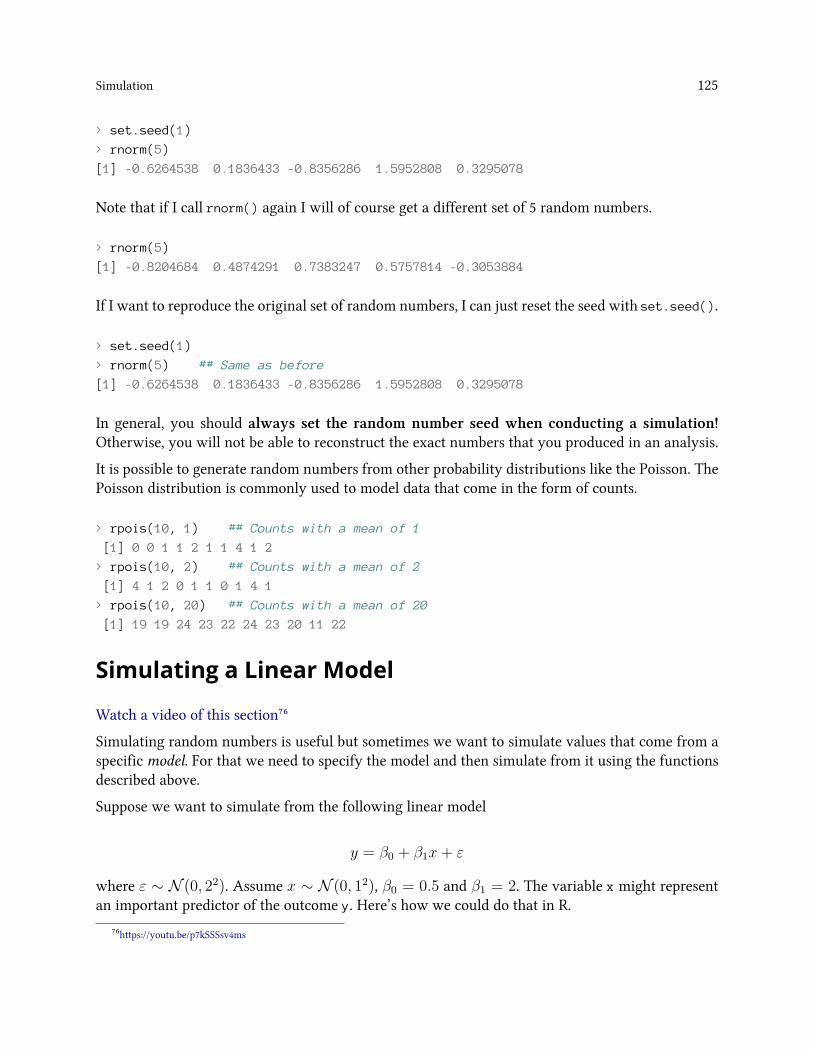
Simulation 125

> set.seed(1)

> rnorm(5)

[1] -0.6264538 0.1836433 -0.8356286 1.5952808 0.3295078

Note that if I call rnorm() again I will of course get a different set of 5 random numbers.

> rnorm(5)

[1] -0.8204684 0.4874291 0.7383247 0.5757814 -0.3053884

If I want to reproduce the original set of random numbers, I can just reset the seed with set.seed().

> set.seed(1)

> rnorm(5) ## Same as before

[1] -0.6264538 0.1836433 -0.8356286 1.5952808 0.3295078

In general, you should always set the random number seed when conducting a simulation!Otherwise, you will not be able to reconstruct the exact numbers that you produced in an analysis.

It is possible to generate random numbers from other probability distributions like the Poisson. ThePoisson distribution is commonly used to model data that come in the form of counts.

> rpois(10, 1) ## Counts with a mean of 1

[1] 0 0 1 1 2 1 1 4 1 2

> rpois(10, 2) ## Counts with a mean of 2

[1] 4 1 2 0 1 1 0 1 4 1

> rpois(10, 20) ## Counts with a mean of 20

[1] 19 19 24 23 22 24 23 20 11 22

Simulating a Linear Model

Watch a video of this section⁷⁶

Simulating random numbers is useful but sometimes we want to simulate values that come from aspecific model. For that we need to specify the model and then simulate from it using the functionsdescribed above.

Suppose we want to simulate from the following linear model

y = β0 + β1x+ ε

where ε ∼ N (0, 22). Assume x ∼ N (0, 12), β0 = 0.5 and β1 = 2. The variable x might representan important predictor of the outcome y. Here’s how we could do that in R.

⁷⁶https://youtu.be/p7kSSSsv4ms

Simulation 126

> ## Always set your seed!

> set.seed(20)

>

> ## Simulate predictor variable

> x <- rnorm(100)

>

> ## Simulate the error term

> e <- rnorm(100, 0, 2)

>

> ## Compute the outcome via the model

> y <- 0.5 + 2 * x + e

> summary(y)

Min. 1st Qu. Median Mean 3rd Qu. Max.

-6.4080 -1.5400 0.6789 0.6893 2.9300 6.5050

We can plot the results of the model simulation.

> plot(x, y)

plot of chunk Linear Model

Simulation 127

What if we wanted to simulate a predictor variable x that is binary instead of having a Normaldistribution. We can use the rbinom() function to simulate binary random variables.

> set.seed(10)

> x <- rbinom(100, 1, 0.5)

> str(x) ## 'x' is now 0s and 1s

int [1:100] 1 0 0 1 0 0 0 0 1 0 ...

Then we can procede with the rest of the model as before.

> e <- rnorm(100, 0, 2)

> y <- 0.5 + 2 * x + e

> plot(x, y)

plot of chunk Linear Model Binary

We can also simulate from generalized linear model where the errors are no longer from a Normaldistribution but come from some other distribution. For examples, suppose we want to simulatefrom a Poisson log-linear model where

Y ∼ Poisson(µ)

Simulation 128

logµ = β0 + β1x

and β0 = 0.5 and β1 = 0.3. We need to use the rpois() function for this

> set.seed(1)

>

> ## Simulate the predictor variable as before

> x <- rnorm(100)

Now we need to compute the log mean of the model and then exponentiate it to get the mean topass to rpois().

> log.mu <- 0.5 + 0.3 * x

> y <- rpois(100, exp(log.mu))

> summary(y)

Min. 1st Qu. Median Mean 3rd Qu. Max.

0.00 1.00 1.00 1.55 2.00 6.00

> plot(x, y)

plot of chunk Poisson Log-Linear Model

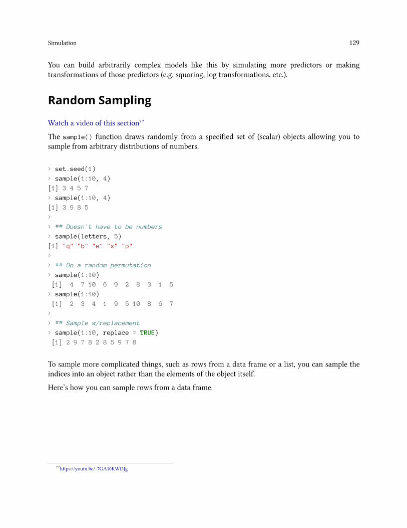
Simulation 129

You can build arbitrarily complex models like this by simulating more predictors or makingtransformations of those predictors (e.g. squaring, log transformations, etc.).

Random Sampling

Watch a video of this section⁷⁷

The sample() function draws randomly from a specified set of (scalar) objects allowing you tosample from arbitrary distributions of numbers.

> set.seed(1)

> sample(1:10, 4)

[1] 3 4 5 7

> sample(1:10, 4)

[1] 3 9 8 5

>

> ## Doesn't have to be numbers

> sample(letters, 5)

[1] "q" "b" "e" "x" "p"

>

> ## Do a random permutation

> sample(1:10)

[1] 4 7 10 6 9 2 8 3 1 5

> sample(1:10)

[1] 2 3 4 1 9 5 10 8 6 7

>

> ## Sample w/replacement

> sample(1:10, replace = TRUE)

[1] 2 9 7 8 2 8 5 9 7 8

To sample more complicated things, such as rows from a data frame or a list, you can sample theindices into an object rather than the elements of the object itself.

Here’s how you can sample rows from a data frame.

⁷⁷https://youtu.be/-7GA10KWDJg

Simulation 130

> library(datasets)

> data(airquality)

> head(airquality)

Ozone Solar.R Wind Temp Month Day

1 41 190 7.4 67 5 1

2 36 118 8.0 72 5 2

3 12 149 12.6 74 5 3

4 18 313 11.5 62 5 4

5 NA NA 14.3 56 5 5

6 28 NA 14.9 66 5 6

Nowwe just need to create the index vector indexing the rows of the data frame and sample directlyfrom that index vector.

> set.seed(20)

>

> ## Create index vector

> idx <- seq_len(nrow(airquality))

>

> ## Sample from the index vector

> samp <- sample(idx, 6)

> airquality[samp, ]

Ozone Solar.R Wind Temp Month Day

135 21 259 15.5 76 9 12

117 168 238 3.4 81 8 25

43 NA 250 9.2 92 6 12

80 79 187 5.1 87 7 19

144 13 238 12.6 64 9 21

146 36 139 10.3 81 9 23

Other more complex objects can be sampled in this way, as long as there’s a way to index the sub-elements of the object.

Summary

• Drawing samples from specific probability distributions can be done with “r” functions• Standard distributions are built in: Normal, Poisson, Binomial, Exponential, Gamma, etc.• The sample() function can be used to draw random samples from arbitrary vectors• Setting the random number generator seed via set.seed() is critical for reproducibility

Data Analysis Case Study: Changes inFine Particle Air Pollution in the U.S.This chapter presents an example data analysis looking at changes in fine particulate matter (PM) airpollution in the United States using the Environmental Protection Agencies freely available nationalmonitoring data. The purpose of the chapter is to just show how the various tools that we havecovered in this book can be used to read, manipulate, and summarize data so that you can developstatistical evidence for relevant real-world questions.

Watch a video of this chapter⁷⁸

Synopsis

In this chapter we aim to describe the changes in fine particle (PM∼2.5∼) outdoor air pollutionin the United States between the years 1999 and 2012. Our overall hypothesis is that out doorPM∼2.5∼ has decreased on average across the U.S. due to nationwide regulatory requirementsarising from the Clean Air Act. To investigate this hypothesis, we obtained PM∼2.5∼ data fromthe U.S. Environmental Protection Agency which is collected from monitors sited across the U.S.We specifically obtained data for the years 1999 and 2012 (the most recent complete year available).From these data, we found that, on average across the U.S., levels of PM∼2.5∼ have decreasedbetween 1999 and 2012. At one individual monitor, we found that levels have decreased and thatthe variability of PM∼2.5∼ has decreased. Most individual states also experienced decreases inPM∼2.5∼, although some states saw increases.

Loading and Processing the Raw Data

From the EPA Air Quality System⁷⁹ we obtained data on fine particulate matter air pollution(PM∼2.5∼) that is monitored across the U.S. as part of the nationwide PM monitoring network.We obtained the files for the years 1999 and 2012.

Reading in the 1999 data

We first read in the 1999 data from the raw text file included in the zip archive. The data is a delimitedfile were fields are delimited with the | character adn missing values are coded as blank fields. Weskip some commented lines in the beginning of the file and initially we do not read the header data.

⁷⁸https://youtu.be/VE-6bQvyfTQ⁷⁹http://www.epa.gov/ttn/airs/airsaqs/detaildata/downloadaqsdata.htm

Data Analysis Case Study: Changes in Fine Particle Air Pollution in the U.S. 132

> pm0 <- read.table("pm25_data/RD_501_88101_1999-0.txt", comment.char = "#", hea\

der = FALSE, sep = "|", na.strings = "")

After reading in the 1999 we check the first few rows (there are 117,421) rows in this dataset.

> dim(pm0)

[1] 117421 28

> head(pm0[, 1:13])

V1 V2 V3 V4 V5 V6 V7 V8 V9 V10 V11 V12 V13

1 RD I 1 27 1 88101 1 7 105 120 19990103 00:00 NA

2 RD I 1 27 1 88101 1 7 105 120 19990106 00:00 NA

3 RD I 1 27 1 88101 1 7 105 120 19990109 00:00 NA

4 RD I 1 27 1 88101 1 7 105 120 19990112 00:00 8.841

5 RD I 1 27 1 88101 1 7 105 120 19990115 00:00 14.920

6 RD I 1 27 1 88101 1 7 105 120 19990118 00:00 3.878

We then attach the column headers to the dataset and make sure that they are properly formatedfor R data frames.

> cnames <- readLines("pm25_data/RD_501_88101_1999-0.txt", 1)

> cnames <- strsplit(cnames, "|", fixed = TRUE)

> ## Ensure names are properly formatted

> names(pm0) <- make.names(cnames[[1]])

> head(pm0[, 1:13])

X..RD Action.Code State.Code County.Code Site.ID Parameter POC

1 RD I 1 27 1 88101 1

2 RD I 1 27 1 88101 1

3 RD I 1 27 1 88101 1

4 RD I 1 27 1 88101 1

5 RD I 1 27 1 88101 1

6 RD I 1 27 1 88101 1

Sample.Duration Unit Method Date Start.Time Sample.Value

1 7 105 120 19990103 00:00 NA

2 7 105 120 19990106 00:00 NA

3 7 105 120 19990109 00:00 NA

4 7 105 120 19990112 00:00 8.841

5 7 105 120 19990115 00:00 14.920

6 7 105 120 19990118 00:00 3.878

The column we are interested in is the Sample.Value column which contains the PM∼2.5∼measurements. Here we extract that column and print a brief summary.

Data Analysis Case Study: Changes in Fine Particle Air Pollution in the U.S. 133

> x0 <- pm0$Sample.Value

> summary(x0)

Min. 1st Qu. Median Mean 3rd Qu. Max. NA's

0.00 7.20 11.50 13.74 17.90 157.10 13217

Missing values are a common problem with environmental data and so we check to se whatproportion of the observations are missing (i.e. coded as NA).

> mean(is.na(x0)) ## Are missing values important here?

[1] 0.1125608

Because the proportion of missing values is relatively low (0.1125608), we choose to ignore missingvalues for now.

Reading in the 2012 data

We then read in the 2012 data in the same manner in which we read the 1999 data (the data files arein the same format).

> pm1 <- read.table("pm25_data/RD_501_88101_2012-0.txt", comment.char = "#",

+ header = FALSE, sep = "|", na.strings = "", nrow = 1304290)

We also set the column names (they are the same as the 1999 dataset) and extract the Sample.Valuecolumn from this dataset.

> names(pm1) <- make.names(cnames[[1]])

> x1 <- pm1$Sample.Value

Results

Entire U.S. analysis

In order to show aggregate changes in PM across the entire monitoring network, we can makeboxplots of all monitor values in 1999 and 2012. Here, we take the log of the PM values to adjust forthe skew in the data.

Data Analysis Case Study: Changes in Fine Particle Air Pollution in the U.S. 134

> boxplot(log2(x0), log2(x1))

Warning in boxplot.default(log2(x0), log2(x1)): NaNs produced

Warning in bplt(at[i], wid = width[i], stats = z$stats[, i], out =

z$out[z$group == : Outlier (-Inf) in boxplot 1 is not drawn

Warning in bplt(at[i], wid = width[i], stats = z$stats[, i], out =

z$out[z$group == : Outlier (-Inf) in boxplot 2 is not drawn

plot of chunk boxplot log values

> summary(x0)

Min. 1st Qu. Median Mean 3rd Qu. Max. NA's

0.00 7.20 11.50 13.74 17.90 157.10 13217

> summary(x1)

Min. 1st Qu. Median Mean 3rd Qu. Max. NA's

-10.00 4.00 7.63 9.14 12.00 909.00 73133

Interestingly, from the summary of x1 it appears there are some negative values of PM, which ingeneral should not occur. We can investigate that somewhat to see if there is anything we shouldworry about.

Data Analysis Case Study: Changes in Fine Particle Air Pollution in the U.S. 135

> negative <- x1 < 0

> mean(negative, na.rm = T)

[1] 0.0215034

There is a relatively small proportion of values that are negative, which is perhaps reassuring. Inorder to investigate this a step further we can extract the date of each measurement from the originaldata frame. The idea here is that perhaps negative values occur more often in some parts of the yearthan other parts. However, the original data are formatted as character strings so we convert themto R’s Date format for easier manipulation.

> dates <- pm1$Date

> dates <- as.Date(as.character(dates), "%Y%m%d")

We can then extract the month from each of the dates with negative values and attempt to identifywhen negative values occur most often.

> missing.months <- month.name[as.POSIXlt(dates)$mon + 1]

> tab <- table(factor(missing.months, levels = month.name))

> round(100 * tab / sum(tab))

January February March April May June July

15 13 15 13 14 13 8

August September October November December

6 3 0 0 0

From the table above it appears that bulk of the negative values occur in the first six months ofthe year (January–June). However, beyond that simple observation, it is not clear why the negativevalues occur. That said, given the relatively low proportion of negative values, we will ignore themfor now.

Changes in PM levels at an individual monitor

So far we have examined the change in PM levels on average across the country. One issue with theprevious analysis is that the monitoring network could have changed in the time period between1999 and 2012. So if for some reason in 2012 there are more monitors concentrated in cleaner partsof the country than there were in 1999, it might appear the PM levels decreased when in fact theydidn’t. In this section we will focus on a single monitor in New York State to see if PM levels at thatmonitor decreased from 1999 to 2012.

Our first task is to identify a monitor in New York State that has data in 1999 and 2012 (not allmonitors operated during both time periods). First we subset the data frames to only include datafrom New York (State.Code == 36) and only include the County.Code and the Site.ID (i.e. monitornumber) variables.

Data Analysis Case Study: Changes in Fine Particle Air Pollution in the U.S. 136

> site0 <- unique(subset(pm0, State.Code == 36, c(County.Code, Site.ID)))

> site1 <- unique(subset(pm1, State.Code == 36, c(County.Code, Site.ID)))

Then we create a new variable that combines the county code and the site ID into a single string.

> site0 <- paste(site0[,1], site0[,2], sep = ".")

> site1 <- paste(site1[,1], site1[,2], sep = ".")

> str(site0)

chr [1:33] "1.5" "1.12" "5.73" "5.80" "5.83" "5.110" ...

> str(site1)

chr [1:18] "1.5" "1.12" "5.80" "5.133" "13.11" "29.5" ...

Finaly, we want the intersection between the sites present in 1999 and 2012 so that we might choosea monitor that has data in both periods.

> both <- intersect(site0, site1)

> print(both)

[1] "1.5" "1.12" "5.80" "13.11" "29.5" "31.3" "63.2008"

[8] "67.1015" "85.55" "101.3"

Here (above) we can see that there are 10 monitors that were operating in both time periods.However, rather than choose one at random, it might best to choose one that had a reasonableamount of data in each year.

> ## Find how many observations available at each monitor

> pm0$county.site <- with(pm0, paste(County.Code, Site.ID, sep = "."))

> pm1$county.site <- with(pm1, paste(County.Code, Site.ID, sep = "."))

> cnt0 <- subset(pm0, State.Code == 36 & county.site %in% both)

> cnt1 <- subset(pm1, State.Code == 36 & county.site %in% both)

Now that we have subsetted the original data frames to only include the data from the monitors thatoverlap between 1999 and 2012, we can split the data frames and count the number of observationsat each monitor to see which ones have the most observations.

Data Analysis Case Study: Changes in Fine Particle Air Pollution in the U.S. 137

> ## 1999

> sapply(split(cnt0, cnt0$county.site), nrow)

1.12 1.5 101.3 13.11 29.5 31.3 5.80 63.2008 67.1015

61 122 152 61 61 183 61 122 122

85.55

7

> ## 2012

> sapply(split(cnt1, cnt1$county.site), nrow)

1.12 1.5 101.3 13.11 29.5 31.3 5.80 63.2008 67.1015

31 64 31 31 33 15 31 30 31

85.55

31

A number of monitors seem suitable from the output, but we will focus here on County 63 and siteID 2008.

> both.county <- 63

> both.id <- 2008

>

> ## Choose county 63 and side ID 2008

> pm1sub <- subset(pm1, State.Code == 36 & County.Code == both.county & Site.ID \

== both.id)

> pm0sub <- subset(pm0, State.Code == 36 & County.Code == both.county & Site.ID \

== both.id)

Now we plot the time series data of PM for the monitor in both years.

> dates1 <- as.Date(as.character(pm1sub$Date), "%Y%m%d")

> x1sub <- pm1sub$Sample.Value

> dates0 <- as.Date(as.character(pm0sub$Date), "%Y%m%d")

> x0sub <- pm0sub$Sample.Value

>

> ## Find global range

> rng <- range(x0sub, x1sub, na.rm = T)

> par(mfrow = c(1, 2), mar = c(4, 5, 2, 1))

> plot(dates0, x0sub, pch = 20, ylim = rng, xlab = "", ylab = expression(PM[2.5]\

* " (" * mu * g/m^3 * ")"))

> abline(h = median(x0sub, na.rm = T))

> plot(dates1, x1sub, pch = 20, ylim = rng, xlab = "", ylab = expression(PM[2.5]\

* " (" * mu * g/m^3 * ")"))

> abline(h = median(x1sub, na.rm = T))

Data Analysis Case Study: Changes in Fine Particle Air Pollution in the U.S. 138

plot of chunk unnamed-chunk-11

From the plot above, we can that median levels of PM (horizontal solid line) have decreased a littlefrom 10.45 in 1999 to 8.29 in 2012. However, perhaps more interesting is that the variation (spread)in the PM values in 2012 is much smaller than it was in 1999. This suggest that not only are medianlevels of PM lower in 2012, but that there are fewer large spikes from day to day. One issue with thedata here is that the 1999 data are from July through December while the 2012 data are recorded inJanuary through April. It would have been better if we’d had full-year data for both years as therecould be some seasonal confounding going on.

Changes in state-wide PM levels

Although ambient air quality standards are set at the federal level in the U.S. and hence affect theentire country, the actual reduction and management of PM is left to the individual states. Statesthat are not “in attainment” have to develop a plan to reduce PM so that that the are in attainment(eventually). Therefore, it might be useful to examine changes in PM at the state level. This analysisfalls somewhere in between looking at the entire country all at once and looking at an individualmonitor.

What we do here is calculate the mean of PM for each state in 1999 and 2012.

> ## 1999

> mn0 <- with(pm0, tapply(Sample.Value, State.Code, mean, na.rm = TRUE))

> ## 2012

> mn1 <- with(pm1, tapply(Sample.Value, State.Code, mean, na.rm = TRUE))

>

> ## Make separate data frames for states / years

> d0 <- data.frame(state = names(mn0), mean = mn0)

> d1 <- data.frame(state = names(mn1), mean = mn1)

> mrg <- merge(d0, d1, by = "state")

> head(mrg)

Data Analysis Case Study: Changes in Fine Particle Air Pollution in the U.S. 139

state mean.x mean.y

1 1 19.956391 10.126190

2 10 14.492895 11.236059

3 11 15.786507 11.991697

4 12 11.137139 8.239690

5 13 19.943240 11.321364

6 15 4.861821 8.749336

Now make a plot that shows the 1999 state-wide means in one “column” and the 2012 state-widemeans in another columns. We then draw a line connecting the means for each year in the samestate to highlight the trend.

> par(mfrow = c(1, 1))

> rng <- range(mrg[,2], mrg[,3])

> with(mrg, plot(rep(1, 52), mrg[, 2], xlim = c(.5, 2.5), ylim = rng, xaxt = "n"\

, xlab = "", ylab = "State-wide Mean PM"))

> with(mrg, points(rep(2, 52), mrg[, 3]))

> segments(rep(1, 52), mrg[, 2], rep(2, 52), mrg[, 3])

> axis(1, c(1, 2), c("1999", "2012"))

plot of chunk unnamed-chunk-13

Data Analysis Case Study: Changes in Fine Particle Air Pollution in the U.S. 140

From the plot above we can see that many states have decreased the average PM levels from 1999to 2012 (although a few states actually increased their levels).