Quick Notes on OG Models - American University · Quick Notes on OG Models Professor: ... 4 The...

Quick Notes on OG Models

Professor: Alan G. Isaac

November 13, 2013

Contents

1 Two-Period Consumption Decision 3

1.1 OG Comparative Statics . . . . . . . . . . . . . . . . . . . . . . . . . . . . 6

2 Firms 9

2.1 Comments . . . . . . . . . . . . . . . . . . . . . . . . . . . . . . . . . . . . 11

2.2 Dynamics . . . . . . . . . . . . . . . . . . . . . . . . . . . . . . . . . . . . 11

3 Social Security 12

3.1 Partial Equilibrium Effects . . . . . . . . . . . . . . . . . . . . . . . . . . . 13

3.2 General Equilibrium Effects . . . . . . . . . . . . . . . . . . . . . . . . . . 14

4 The Golden Rule 15

5 More Cohorts 17

5.0.1 Retired Individuals . . . . . . . . . . . . . . . . . . . . . . . . . . . 18

5.0.2 Working Individuals . . . . . . . . . . . . . . . . . . . . . . . . . . 20

5.1 Path Computation . . . . . . . . . . . . . . . . . . . . . . . . . . . . . . . 22

5.2 Equilibrium . . . . . . . . . . . . . . . . . . . . . . . . . . . . . . . . . . . 23

1

CONTENTS CONTENTS

5.3 HM’s Simulation . . . . . . . . . . . . . . . . . . . . . . . . . . . . . . . . 24

5.3.1 Calibration . . . . . . . . . . . . . . . . . . . . . . . . . . . . . . . 24

Be sure to read the entire Blanchard and Fischer treatment of social security in the

OG model. These notes are purely supplementary.

We turn to the overlapping generations (OG) model at this point because of two

primary virtues.

� it allows exploration of the implications of life-cycle savings in an intergenerational

world. We will focus in particular on the savings and investment repercussions of

social security systems.

� it shows how competitive equilibrium may not be Pareto optimal.

Copyright © 2013 by Alan G. Isaac 2

1 TWO-PERIOD CONSUMPTION DECISION

1 Two-Period Consumption Decision

We initially simplify in three important ways: two-periods lives, no uncertainty, and

no labor/leisure trade-off. Inelastically supplied labor means that in the individual’s

optimization problem we can treat labor income as exogenous.

An individual born at time t lives two periods, t and t + 1. Given initial wealth a0,

her basic optimization problem is to

maxc0,c1,a2

U(c0, c1, a2) (1)

subject to the constraints

a1 = R0,1(a0 + y0 − c0) a2 = R1,2(a1 + y1 − c1) (2)

Here yt is income and ct is consumption. These take place at the beginning of the period,

and Rt,t+1 is the gross interest rate applying over the period. (Later we will just call this

Rt+1, but for now we want to emphasize the timing.)

Arithmetically, we can combine these two constraints by eliminating a1:

c0 + c1/R0,1 + a2/R0,1R1,2 = a0 + y0 + y1/R0,1 (3)

That is, in present value terms, the total value of “expenditures” must equal the total

value of available resources (w0 = a0 + y0 + y1/R0,1, i.e., initial wealth plus labor income).

If capital markets allow unrestricted borrowing and lending at the prevailing interest rate,

so that there is no effective constraint on the value of a1, then this single constraint is

adequate for the consumer optimization problem. This means that the timing of con-

sumption does not depend on the timing of income: only the present value of the income

stream is relevant to the consumption decision.



We should consider two additional constraints: ct ≥ 0 and a2 ≥ 0. The first is an

essentially a physical constraint: negative consumption is not possible. We generally

(directly or indirectly) assume that this constraint is not binding. We may need the

second constraint to rule out consumer plans to die in debt. For now we will simplify the

utility function to U(c0, c1) and set a0 = a2 = 0. Our problem becomes

maxc0,c1

U(c0, c1) s.t. c0 + c1/R0,1 = y0 + y1/R0,1 (4)

Note that when we can aggregate the single period budget constraints, it becomes

clear that there is nothing inherently dynamic in the optimization problem. Think of the

price of first period consumption as 1 and the price of second period consumption as 1/R.

Then it is essentially our familiar two-good consumer choice problem.

maxcU(c) s.t. p · c = w (5)

where

c = (c0, c1) p = (1, 1/R0,1) w = a0 + y0 + y1/R0,1 (6)

As an algebraic convenience, let us transform this constrained optimization problem

into an unconstrained optimization by defining s = y0 − c0. Our problem becomes

maxsU(y0 − s, R0,1s+ y1) (7)

The first-order necessary condition for an optimum is then

−U0 +R0,1U1 = 0 (8)

This is just the standard Fisher equality between the marginal rate of substitution and



the gross return to investment.

U0/U1 = R0,1 (9)

It has become more common to write this condition as

U0 = R0,1U1 (10)

and call it an Euler condition. The Euler condition relates the marginal utility of con-

sumption in adjacent periods.

Now we will add structure to our model. Our consumer works when young and lives

off her savings when old. This further simplifies the buget contraint: there is no labor

income when old.

maxU(c0, c1) s.t. c0 + c1/R0,1 = y0 (11)

Figure 1 presents the solution of this optimization problem for two different levels

of the interest rate. Clearly an increase in the interest rate generate has two conflicting

effects on first period consumption. First, it is a change in the relative price: consumption

when young now involves a larger sacrifice of consumption when old, so there is a tendency

to postpone consumption. On the other hand, a higher interest rate raises real income,

which tends to increase consumption in both periods. On net, we do not know whether

consumption rises or falls in response to an interest rate increase. Since saving is just

s(w,R) = w − c0(w,R), we also do not know whether saving increases or decreases.

The effects of an exogenous increase in wage income are easier to pin down. An

increase in y0 simply shifts the budget constraint outward, without changing the slope.

As long as both goods are normal, some of this increase in income will be allocated toward

consumption when old. As a result, saving is increasing in w.


1.1 OG Comparative Statics 1 TWO-PERIOD CONSUMPTION DECISION

c1

c0

eeeeeeeeeeee U

JJJJJJJJJJJJJJJ

U ′

c0 y0

Ry0

R′y0

Figure 1: Two Period Consumption Decision

1.1 OG Comparative Statics

Next we will examine the comparative statics algebraically. It will simplify things a bit if

we adopt the following popular time-separable utility function:

U(c0, c1) = u(c0) + βu(c1)

=1∑t=0

βtu(ct)(12)

Note that u(·) is the same each period. We will assume that in each period marginal

utility is positive and decreasing: u′ > 0 and u′′ < 0. Note that we follow Irving Fisher in

assuming people are impatient: consumption in the present period yields more utility than

the same consumption in a future period (from the point of view of present planning).

Here 0 < β < 1 is the discount factor.1 The assumption that β < 1 is the assumption that

the rate of time preference is positive: consumers would prefer to shift a perfectly smooth

1The discount factor β is related to the rate of time preference θ according to β = 1/(1 + θ). Theassumption that β < 1 is the assumption that the rate of time preference is positive: consumers wouldprefer to shift a perfectly smooth consumption stream toward the present (if there were no costs in totalconsumption).



consumption stream toward the present (if there were no costs in total consumption).

Exercise 1

Consumption of a normal good is increasing in income. Prove that additivity along with

concavity of u(·) implies that each period’s consumption is normal.

With time separable, discounted utility, the consumer’s maximization problem be-

comes

maxsu(y0 − s) + βu(R0,1s) (13)

with first-order condition

u′0/βu′1 = R0,1 (14)

or equivalently

u′0/u′1 = R0,1β (15)

Exercise 2

Show that a second-order sufficient condition is satified.

So whether the consumption stream is actually tilted toward youth depends on the

relative size of R and β. Equivalently, if we write R = 1 + r and β = 1/(1 + θ), it depends

on the size of the interest rater (r) relative to the rate of time preference (θ). If the

interest rate is high enough, it can pay to tilt your consumption profile toward old age:

total physical consumption increases enough to offset impatience. If θ = r (i.e., Rβ = 1)

then consumption is constant across the two periods.

Exercise 3

Note that separability and concavity of u(·) imply each period’s consumption is normal.

(You should prove this.) Do we use separability anywhere? Or just normality?

More explicitly, the first order condition is

−u′(y0 − s) +R0,1βu′(R0,1s) = 0 (16)



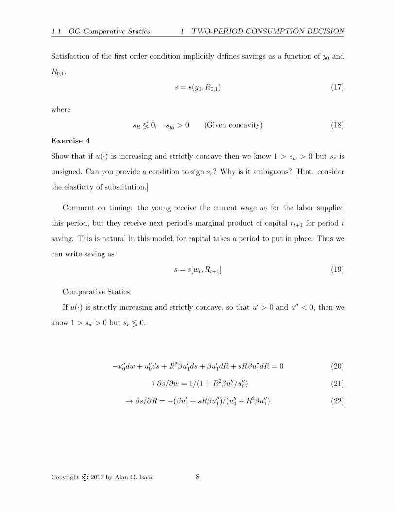
Satisfaction of the first-order condition implicitly defines savings as a function of y0 and

R0,1.

s = s(y0, R0,1) (17)

where

sR ≶ 0, sy0 > 0 (Given concavity) (18)

Exercise 4

Show that if u(·) is increasing and strictly concave then we know 1 > sw > 0 but sr is

unsigned. Can you provide a condition to sign sr? Why is it ambiguous? [Hint: consider

the elasticity of substitution.]

Comment on timing: the young receive the current wage wt for the labor supplied

this period, but they receive next period’s marginal product of capital rt+1 for period t

saving. This is natural in this model, for capital takes a period to put in place. Thus we

can write saving as

s = s[wt, Rt+1] (19)

Comparative Statics:

If u(·) is strictly increasing and strictly concave, so that u′ > 0 and u′′ < 0, then we

know 1 > sw > 0 but sr ≶ 0.

−u′′0dw + u′′0ds+R2βu′′1ds+ βu′1dR + sRβu′′1dR = 0 (20)

→ ∂s/∂w = 1/(1 +R2βu′′1/u′′0) (21)

→ ∂s/∂R = −(βu′1 + sRβu′′1)/(u′′0 +R2βu′′1) (22)


2 FIRMS

2 Firms

All costs of adjustment are ignored. Individual firms choose their optimal level of N and

K each period. (Note, however, that in the aggregate N and K are predetermined.)

maxK,N

F (K,N)− wN − rK (23)

yields the FOCs

FK(Kd, Nd) = r (24)

FN(Kd, Nd) = w (25)

which can be solved for

Nd = N(w, r) (26)

Kd = K(w, r) (27)

Assume CRTS production: F (λK, λN) ≡ λF (K,N). In this case, total product exactly

exhausted when factors are paid their marginal products.

Define k ≡ K/N and f(k) ≡ F (k, 1) = (1/N)F (K,N). Then

F (K,N) ≡ Nf(K/N)

FK = N1

Nf ′ = f ′

FN = f −Nf ′K/N2 = f − kf ′


2 FIRMS

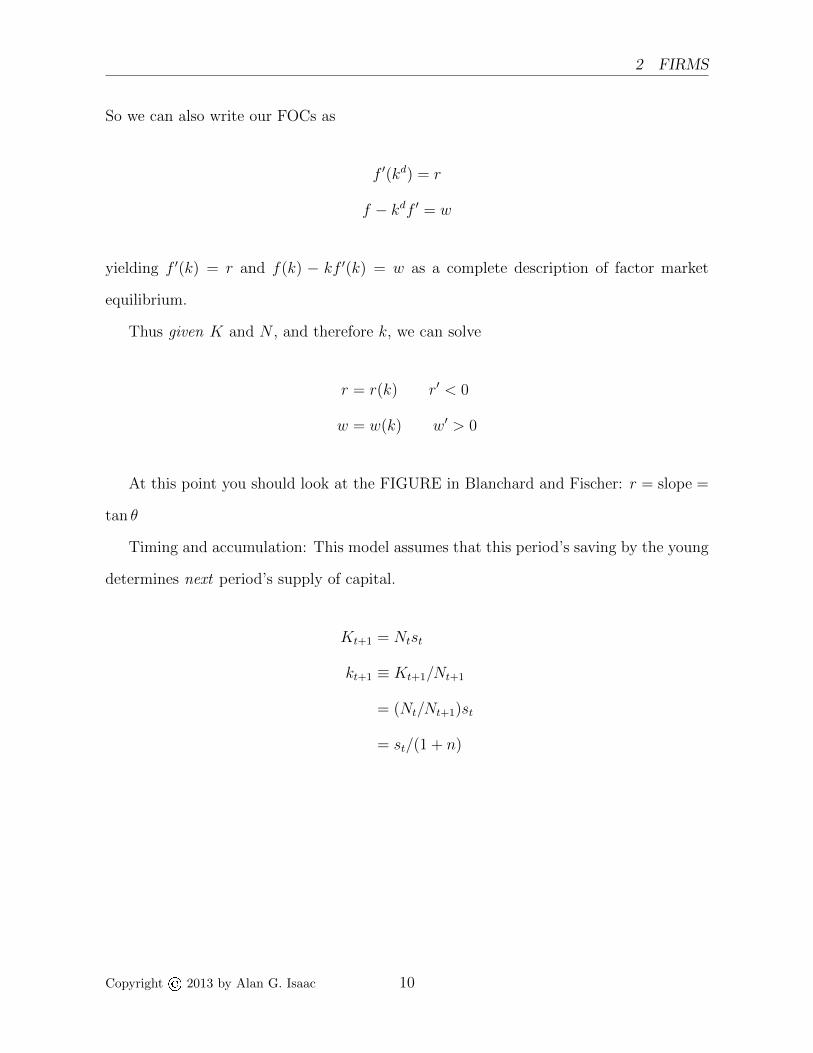
So we can also write our FOCs as

f ′(kd) = r

f − kdf ′ = w

yielding f ′(k) = r and f(k) − kf ′(k) = w as a complete description of factor market

equilibrium.

Thus given K and N , and therefore k, we can solve

r = r(k) r′ < 0

w = w(k) w′ > 0

At this point you should look at the FIGURE in Blanchard and Fischer: r = slope =

tan θ

Timing and accumulation: This model assumes that this period’s saving by the young

determines next period’s supply of capital.

Kt+1 = Ntst

kt+1 ≡ Kt+1/Nt+1

= (Nt/Nt+1)st

= st/(1 + n)


2.1 Comments 2 FIRMS

2.1 Comments

1) Only the young save, the old dissave. So aggregate saving is

St ≡ Yt − Ct

= F (Kt, Nt)−Ntcyt −Nt−1cot

= F (Kt, Nt)−Nt[wt − st]−Nt−1[RtKt/Nt−1]

= F (Kt, Nt)− wtNt − rtKt︸︷︷︸0

+Ntst −Kt since Rt = 1 + rt

= Ntst −Kt

IF factor markets clear.

Now St ≡ It is an identity ; Kt+1 −Kt = It is an assumption (about units of measure-

ment and depreciation). So

Kt+1 −Kt = Ntst −Kt (28)

2) Given the previous period’s saving decision, you might be tempted to think of both

capital and labor as inelastically supplied in period t. But that saving decision was made

with (perfect foresight) knowledge of rt.

2.2 Dynamics

Recall

kt+1 = st/(1 + n) and st = s(wt, rt+1) (29)

so that

kt+1 = s(wt, rt+1)/(1 + n) (30)


3 SOCIAL SECURITY

where

wt = f(kt)− ktf ′(kt)⇔ wt = w(kt) with w′ > 0

rt+1 = f ′(kt+1)⇔ rt+1 = r(kt+1) with r′ < 0

Thus the dynamic behavior of the economy can be summarized in the following non-

linear difference equation in k.

kt+1 = s[w(kt), r(kt+1)]/(1 + n) (31)

We can derive the slope in (kt+1, kt)-space as follows.

(1 + n)dkt+1 = sww′dkt + srr

′dkt+1

dkt+1 = [sww′t/(1 + n− srr′t+1)]dkt

Don’t Forget: w′ = dw/dkt r′ = dr/dkt+1

Note that dkt+1/dkt > 0 unambiguously IF we make the classical assumption that

sr > 0.

The model doesn’t guarantee existence, uniqueness, or stability of a steady state.

For the moment, let’s assume there is a unique, non-zero k steady state, k∞, and that

1 > dkt+1/dkt > 0 at k∞.

At this point you should look at the relevant GRAPH in Blanchard and Fischer:

3 Social Security

Here we will consider a pay as you go system, which is roughly the US system. Current

collections from young workers δt are fully disbursed to the current old. So the young pay

δt into social security when working and receive (1 + n)δt+1 when retired.


3.1 Partial Equilibrium Effects 3 SOCIAL SECURITY

We continue to think of st as per capita saving by the young at time t out of their

disposable income, which is now wt − δt. We now need to keep track of the consumption

of both the young and the old each period, so we modify our notation accordingly.

The budget constraints becomes

cyt = wt − δt − st cot+1 = Rt+1st + (1 + n)δt+1 (32)

Therefore the problem is

maxsu[wt − δt − st] + βu[Rt+1st + (1 + n)δt+1] (33)

FOC:

−u′0 + βRt+1u′1 = 0⇔ st = s(wt, δt, Rt+1, δt+1) (34)

Let’s assume δt constant at δ so that st = s(wt, Rt+1, δ). Given w and r, we can totally

differentiate the first order condition with respect to s and δ.

u′′yds+ u′′ydδ + βR2u′′ods+ βR(1 + n)u′′odδ = 0 (35)

Using this, we find

∂s

∂δ= −

u′′y + β(1 + n)Ru′′ou′′y + βu′′oR

2(36)

3.1 Partial Equilibrium Effects

1. ∂s/∂δ < 0! Social security decreases individual private saving. [HW: intuition for

this. Hint: note that when δt 6= δt+1, changing either one has the same qualitative

effect on saving, so graph the effect of each of these changes separately.]

2. |∂s/∂δ|><1 as n><r


3.2 General Equilibrium Effects 3 SOCIAL SECURITY

3.2 General Equilibrium Effects

We know

↑ δ ⇔↓ st ⇔↓ kt+1 ⇔↑ rt+1 (37)

but the crucial feedback from rt+1 to st is theoretically ambiguous.

Given kt, what is net (general equilibrium) effect of increase social security payments

(↑ δ) on st (and therefore on kt+1)?

st = s[w(kt), R(kt+1), δ] (38)

Recall

(1 + n)kt+1 = st (39)

So

(1 + n)dkt+1 = sddδ + sRR′dkt+1 (40)

Rearranging, we get

dkt+1/dδ = sd/[1 + n− sRR′] (41)

Since sd < 0, the sign of dkt+1/dδ depends on the denominator 1 +n− sRR′. This can be

interpreted in terms of the slope of the saving and “investment” functions.

At this point you should GRAPH s/(1 + n) vs R and kt+1 vs f ′, noting that the first

has slope sR/(1 + n) and the second has slope 1/R′.

We will assume the denominator is positive (1 + n− sRR′ > 0), so that dkt+1/dδ < 0.

Justification: unique, stable, and non-oscillatory equilibrium requires 0 < dkt+1/dkt < 1.

Recall that

dkt+1

dkt=

sww′t

1 + n− sRR′t+1

(42)

[or, since w′ = −kR′, dkt+1/dkt = −swktR′t/(1+n−sRR′t+1)] so that (1+n−sRR′t+1) > 0


4 THE GOLDEN RULE

is necessary for dkt+1/dkt > 0.

At this point you should GRAPH the shift of the equilibrium accumulation curve

under these assumptions.

Capital accumulation slows, steady state k decreases. Is this bad? Depends on dy-

namic efficiency. See the discussions p. 113 of B&F.

4 The Golden Rule

Recall

Ct = Ntcyt +Nt−1cot (43)

so

c ≡ Ct/Nt = cyt + cot/(1 + n) (44)

or

St = F (Kt, Nt)− Ct ⇔ ct = f(kt)− [syt − kt] (45)

Recall also that

(1 + n)kt+1 = st ⇔ ct = f(kt)− [(1 + n)kt+1 − kt] (46)

So c∞ = f(k∞)− nk∞

Note

dc∞dk∞

= f ′(k∞)− n><0 as f ′(k∞)><n (47)

Golden Rule: f ′(k∞) = n Maximizes Steady State Consumption Per Capita.

HW: Suppose f ′(k)− n > 0. What happens if we steal dk from capital stock at time

t? Show p.103 B & F ct+i > c∞ ∀i > 0.

So we can give dk to period t consumers: all better off


4 THE GOLDEN RULE

Exercise 5

Summarize Blanchard and Fischer’s discussion in section 3.2 of a fully funded social

security system.

Exercise 6

Let F (λK, λN) ≡ λF (K,N). Show that this first degree homogeneity (constant returns

to scale) implies that

FKK + FNN = F (K,N) (48)

so total product exactly exhausted when factors are paid their marginal products. [Hint:

Differentiate w.r.t. λ and evaluate at λ = 1.]

Suggested reading: Blanchard & Fischer ch.3; Silberberg chapter 12.; Allais 1947,

Economie et Interet; Samuelson 1958 JPE 66(6); Diamond 1965 AER 55(5).


5 MORE COHORTS

5 More Cohorts

In this section, we consider a simplified version of Auerbach and Kotlikoff (1987), following

Heer and Maussner (2009).

Households live Tw + T r economic years (working and retirement). The total popula-

tion is normalized to one. So each generation has measure 1/(Tw + T r.

Consider a 60 generation OG model, where Tw = 40 and T r = 20. so each generation

has measure 1/60.


5 MORE COHORTS

5.0.1 Retired Individuals

The value function of an individual depends on the aggregate variables K and N , as wellas on their individual holding k.

Consider a retired individual of generation s. They want to maximize the value ofconsumption over the rest of their lifetime.

V s(ks, Kt, Nt) = maxcu(cs, 1) + βV s+1(ks+1, Kt+1, Nt+1) (49)

For a retired indvidual, the transition equation for k is

ks+1 = (1 + r)ks + b− cs (50)

Plugging into the recursive value equation gives us our Bellman equation:

V s(ks, Kt, Nt) = maxcs

u(cs, 1) + βV s+1((1 + r)ks + b− cs, Kt+1, Nt+1) (51)

First-order condition:0 = ucs − βV s+1

ks+1 (52)

Envelope condition:V sks = (1 + r)βV s+1

ks+1 (53)

Joint implication:(1 + r)ucs = V s

ks (54)

Looking at that one period ahead:

(1 + r)ucs+1 = V s+1ks+1 (55)

Putting these together,ucs = (1 + r)βucs+1 (56)

Note that this is a second-order difference equation in k, as we see by substittuting for cfrom the transition equation.

ucs [(1 + r)ks + b− ks+1, 1] = (1 + r)βucs+1 [(1 + r)ks+1 + b− ks+2, 1] (57)

This is our Euler equation.


5 MORE COHORTS

Suppose an agent is in his first year of retirement, with wealth kTw+1. Then we are

trying to plan 19 values of ks (s = 42, ..., 60) with 19 Euler equations. (Remember,k61 = 0.)

Solution strategy for the retirement path, given a target ks. (Here our target will bethe k for the first year of retirement that is implied by being borh with no beques. (I.e.,our underlying target is k0 = 0.

� set k61 = 0 (dead; no bequests)

� guess k60

� use our Euler equation to work backwards to implied ks

� if implied ks not equal to ks, adjust guess and try again

Given one-period-ahead values for k and c, we can compute deviation from the Eulercondition as follows:

def r f o l d ( k0 , k1 , c1 ) :””” Return f l o a t , d e v i a t i o n from Eu l e r c o n d i t i o n . ( See HM p . 4 6 0 . )

Use t h i s t o f i n d k0 so t h a t Eu l e r c o n d i t i o n s a t s i f i e d .

”””

global pen , beta , rc0 = (1+r ) *k0 + pen − k1return u c ( c0 , 1 ) / beta − u c ( c1 , 1 ) *(1+ r )

Use this to choose k0 so that Euler condition satsified. That is, use the Euler equationerror as a root function in an optimization.

( k0 , ) , , jcode , = f s o l v e ( r f o l d , k1 , args=(k1 , c1 ) , f u l l o u t pu t=True )


5 MORE COHORTS

5.0.2 Working Individuals

We handle working individuals essentially the same way, but they must also choose theirlabor supplies.

Assume there are no bequests, so they are born with 0 wealth.Consider a working individual of generation s. They want to maximize the value of

consumption and leisure over the rest of their lifetime.

V s(ks, `s, Nt, Kt) = maxcu(cs, `s) + βV s+1(ks+1, `s+1, Kt+1, Nt+1) (58)

For a working indvidual, the transition equation for k is

ks+1 = (1 + r)ks + w(1− τ)(1− `)− cs (59)

Plugging into the recursive value equation gives us our Bellman equation:

V s(ks, `s, Nt, Kt) = maxcs,`s

u(cs, `) +βV s+1((1 + r)ks +w(1− τ)(1− `)− cs, `s+1, Kt+1, Nt+1)

(60)We now have two first-order conditions:

0 = ucs − βV s+1ks+1

0 = u`s − βw(1− τ)V s+1ks+1

(61)

The envelope condition is unchanged:

V sks = (1 + r)βV s+1

ks+1 (62)

Our earlier work showed us

(1 + r)ucs+1 = V s+1ks+1 (63)

so our first order conditions imply

ucs = β(1 + r)ucs+1

u`s = w(1− τ)ucs(64)

We can again plug in our transition equation to get a difference equation system in k thatwe will call our Euler equations. Given one-period-ahead values for k, n, and c, we canagain compute deviation from the Euler conditions:

def r f young ( kn0 , k1 , n1 , c1 ) :global beta , rk0 , n0 = kn0c0 = (1+r ) *k0 + (1−tau ) *w*n0 − k1r f 1 = u c ( c0 ,1−n0 ) /beta − u c ( c1 ,1−n1 ) *(1+ r )r f 2 = (1−tau ) *w*u c ( c0 ,1−n0 ) − u e l l ( c0 ,1−n0 )return ( r f1 , r f 2 )


5 MORE COHORTS

Once again, use this to choose k0 so that Euler condition satsified. That is, use theEuler equation error as a root function in an optimization.

( k0 , ) , , jcode , = f s o l v e ( r f young , ( k1 , n1 ) ,\args=(k1 , c1 ) , f u l l o u t pu t=True )


5.1 Path Computation 5 MORE COHORTS

5.1 Path Computation

def pathupdate ( kbar , nbar ) :global nq1 , pen , w, rw = y n ( kbar , nbar ) #c om p e t i t i v e wage

r = y k ( kbar , nbar ) − de l t a #c om p e t i t i v e i n t e r e s t r a t e

#compute p e n s i o n ( g i v e n r e p l a c emen t r a t i o & income t a x r a t e )

pen = rep * (1−tau ) * w * nbar * 3/2 .0

k0 1 , k0 = 0 , 0 #j u s t a d e c l a r a t i o n ; t h e s e v a l u e s aren ' t u s ed

#born w/o wea l t h , so s e e k ( bac kward i n d u c t i o n ) p a t h where k [ 0 ]=0

q1 = 0 ; #maximum i t e r a t i o n s i s nq1 ( i . e . , 30 ) ; f o r c e burn i n

while ( q1 < nq1 ) and ( ( q1<=5) or ( abs ( k0 )>=to l k ) ) :q1 = q1 + 1i f q1 > nq1 :

print "WARNING: kpath(kbar,nbar) convergence failed"

breaki f verbose : print "iteration {} over q1:" . format ( q1 )

#upda t e f i n a l a s s e t l e v e l ( u s e HM ' s i n i t i a l v a l s )

i f q1==1: k60 = 0.15e l i f q1==2: k60 1 , k60 = k60 , 0 . 2else : k60 1 , k60 = k60 , updat e k l a s t ( k60 1 , k0 1 , k60 , k0 )

# NOW, g i v e n k60 , work b a c kwa r d s t o k0 ( h o p i n g f o r 0) .

### FIRST , compute o p t im a l r e t i r e d d e c i s i o n s ( wo r k i n g

. . . b a c kwa r d s ) .

kpath = kpath o ld ( r f o l d , k60 , 0 , tr −1) #( no b e q u e s t )

### SECOND, compute t h e o p t im a l d e c i s i o n s w h i l e wo r k i n g .

### (Remember , r e t i rmemen t y e a r s d e t e rm i n e d a bo v e . )

knpaths = kpath yng ( r f young , kpath [−1] , kpath [−2] , 40)kpath . extend ( knpaths [ 0 ] )

k0 1 , k0 = k0 , kpath [−1]i f True : print ”””

q : { q } q1 : { q1 } k0 : { k0 } k l a s t : { k l a s t }””” . format (q=q , q1=q1 , k0=kpath [−1] , k l a s t=kpath [ 1 ] )return kpath [ : : − 1 ] , knpaths [ 1 ] [ : : − 1 ]


5.2 Equilibrium 5 MORE COHORTS

5.2 Equilibrium

Aggregate production: each period is

Y = KαN1−α (65)

Equilibrium requires

� Consistency of individual behavior and aggregate outcomes:

Nt =Tw∑s=1

nstTw + T r

Kt =Tw+T r∑s=1

kstTw + T r

Note that these sums are weighted by the appropriate population masses.

� Competitive factor markets clear each period:

w = (1− α)(K/N)α r = α(N/K)1−α − d

� Satisfaction of the consumers’ Euler conditions.

� Goods market clearingF (N,K) = C + I

where

C =T 2+T r∑s=1

cs

TW + T rI = K+1 − (1− d)K

� The government budget constraint is satisfied

τwN = bT r

T r + Tw

Note on the government budget constraint: The budget is balanced each period. Taxesfinance retirement pensions of b per retiree. Note total pension expenditure is multipliedby the fraction of the population receiving benefits, because the population has beennormalized to 1.


5.3 HM’s Simulation 5 MORE COHORTS

Macro solution strategy:

� guess K and N ,

� iteration step: solve optimization for the implied Knew and Nnew

� while the change is too big, set (K,N)← (Knew,Nnew) and repeat the iteration step

kpath , npath = pathupdate ( kbar , nbar )#s t o r e o l d K & N, t h en up d a t e K & N ( b u t no t t o o f a s t )

kold , nold = kbar , nbarkbar = phi * kold + (1−phi ) *np .mean( kpath )nbar = phi *nold + (1−phi ) *np .mean( npath ) *2/3

5.3 HM’s Simulation

In HM, tility is dervied from consumption (c) and leisure (`) according to

u(c, `) =((c+ ψ)`γ)1−η − 1

1− η(66)

5.3.1 Calibration

HM’s parameter values

� η = 2

� β = 0.99

� α = 0.3

� d = 0.1

� Tw = 40

� T r = 20

� γ = 2.0

� rep = 0.3

� τ = rep/(2 + rep)

� ψ = 0.001

Comment on the replacement ratio:

rep =b

(1− τ)wn(67)

is set to 0.3. The pension b is an implied value.


Quick Notes on OG Models - American University · Quick Notes on OG Models Professor: ... 4 The...

Documents

Transcript of Quick Notes on OG Models - American University · Quick Notes on OG Models Professor: ... 4 The...