Query Processing & Optimization - Joyce Hojoyceho.github.io/cs377_s17/slide/22-23-query-opt.pdf ·...
88
Query Processing & Optimization CS 377: Database Systems
Transcript of Query Processing & Optimization - Joyce Hojoyceho.github.io/cs377_s17/slide/22-23-query-opt.pdf ·...
Query Processing & OptimizationCS 377: Database Systems

CS 377 [Spring 2017] - Ho
Recap: File Organization & Indexing• Physical level support for data retrieval
• File organization: ordered or sequential file to find items using binary search
• Index: data structures to help with some query evaluation (selection & range queries)
• Indexes may not always be useful even for selection queries
• What about join queries and other queries not supported by indices?
CS 377 [Spring 2017] - Ho
Query Processing Introduction
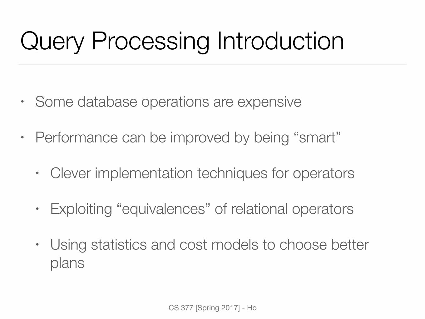
• Some database operations are expensive
• Performance can be improved by being “smart”
• Clever implementation techniques for operators
• Exploiting “equivalences” of relational operators
• Using statistics and cost models to choose better plans

queryoutput
query parser andtranslator
evaluation engine
relational-algebraexpression
execution plan
optimizer
data statisticsabout data
Basic Steps in Query Processing
• Parse and translate: convert to RA query
• Optimize RA query based on the different possible plans
• Evaluate the execution plan to obtain the query results
Figure 12.1 from Database System Concepts book
CS 377 [Spring 2017] - Ho
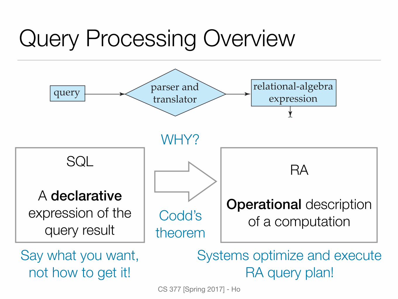
Query Processing Overview
queryoutput
query parser andtranslator
evaluation engine
relational-algebraexpression
execution plan
optimizer
data statisticsabout data
SQL
A declarative expression of the
query result
RA
Operational description of a computation
WHY?
Systems optimize and execute RA query plan!
Say what you want, not how to get it!
Codd’s theorem

CS 377 [Spring 2017] - Ho
Example: SQL Query
Find movies with stars born in 1960
SELECT movieTitle FROM StarsIn, MovieStar WHERE starName = nameAND birthdate LIKE ‘%1960’;
CS 377 [Spring 2017] - Ho
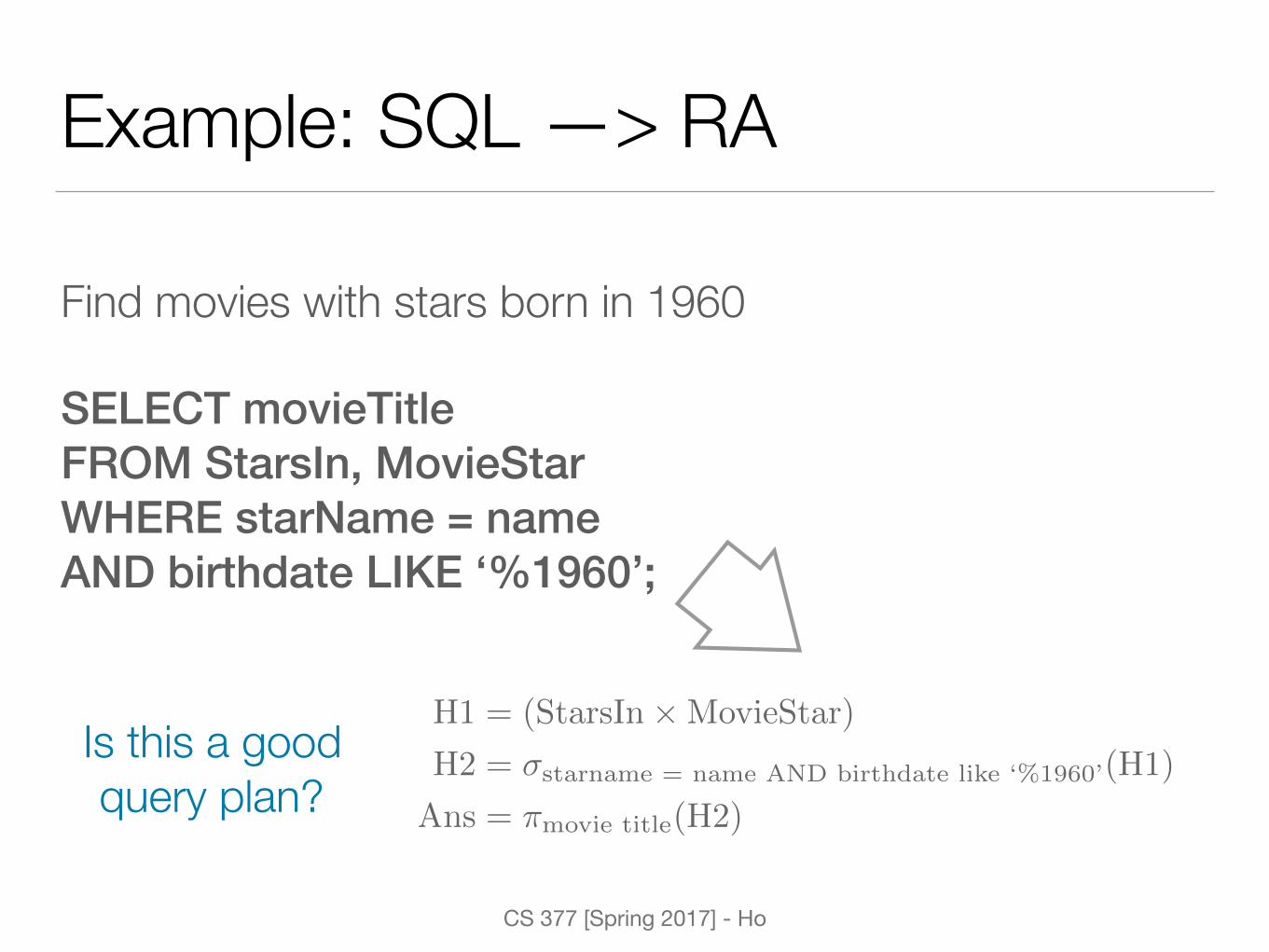
Example: SQL —> RA
Find movies with stars born in 1960
SELECT movieTitle FROM StarsIn, MovieStar WHERE starName = nameAND birthdate LIKE ‘%1960’;
H1 = (StarsIn⇥MovieStar)
H2 = �starname = name AND birthdate like ‘%1960’
(H1)
Ans = ⇡movie title
(H2)
Is this a good query plan?
CS 377 [Spring 2017] - Ho
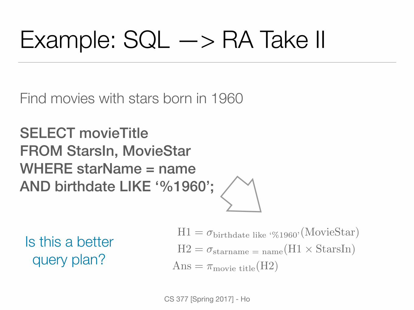
Example: SQL —> RA Take II
Find movies with stars born in 1960
SELECT movieTitle FROM StarsIn, MovieStar WHERE starName = nameAND birthdate LIKE ‘%1960’;
Is this a better query plan?
H1 = �birthdate like ‘%1960’
(MovieStar)
H2 = �starname = name
(H1⇥ StarsIn)
Ans = ⇡movie title
(H2)
CS 377 [Spring 2017] - Ho
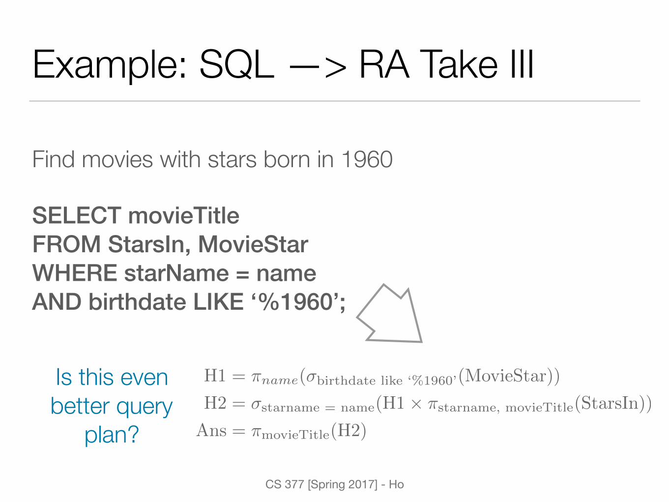
Example: SQL —> RA Take III
Find movies with stars born in 1960
SELECT movieTitle FROM StarsIn, MovieStar WHERE starName = nameAND birthdate LIKE ‘%1960’;
Is this even better query
plan?
H1 = ⇡name(�birthdate like ‘%1960’
(MovieStar))
H2 = �starname = name
(H1⇥ ⇡starname, movieTitle
(StarsIn))
Ans = ⇡movieTitle
(H2)
CS 377 [Spring 2017] - Ho
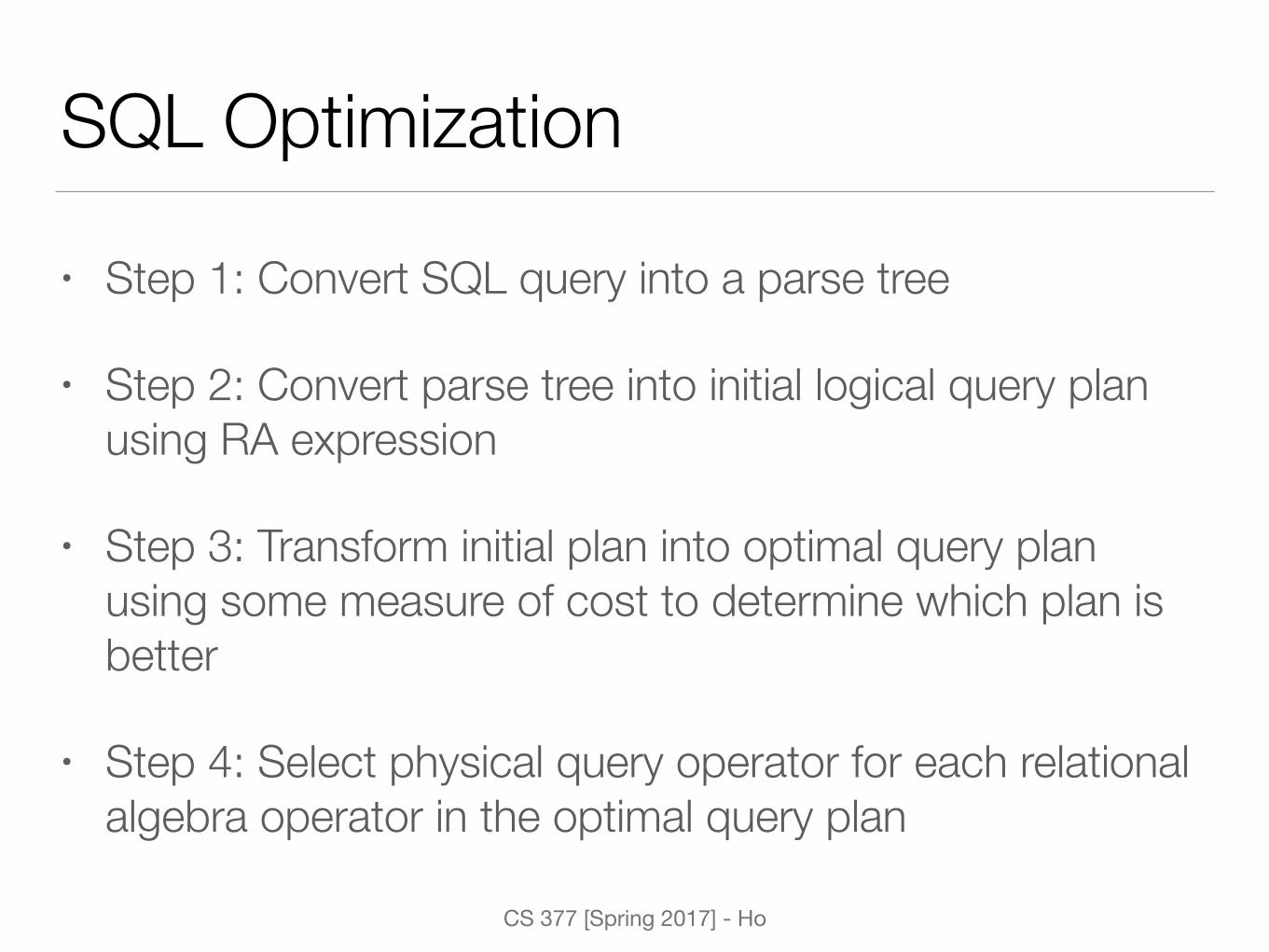
SQL Optimization
• Step 1: Convert SQL query into a parse tree
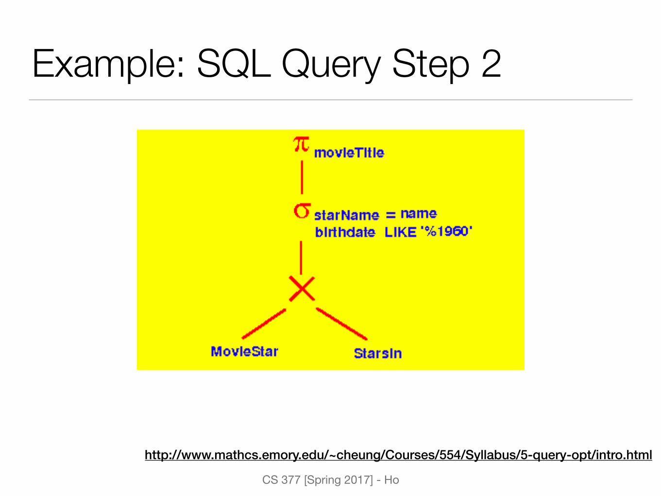
• Step 2: Convert parse tree into initial logical query plan using RA expression
• Step 3: Transform initial plan into optimal query plan using some measure of cost to determine which plan is better
• Step 4: Select physical query operator for each relational algebra operator in the optimal query plan
CS 377 [Spring 2017] - Ho
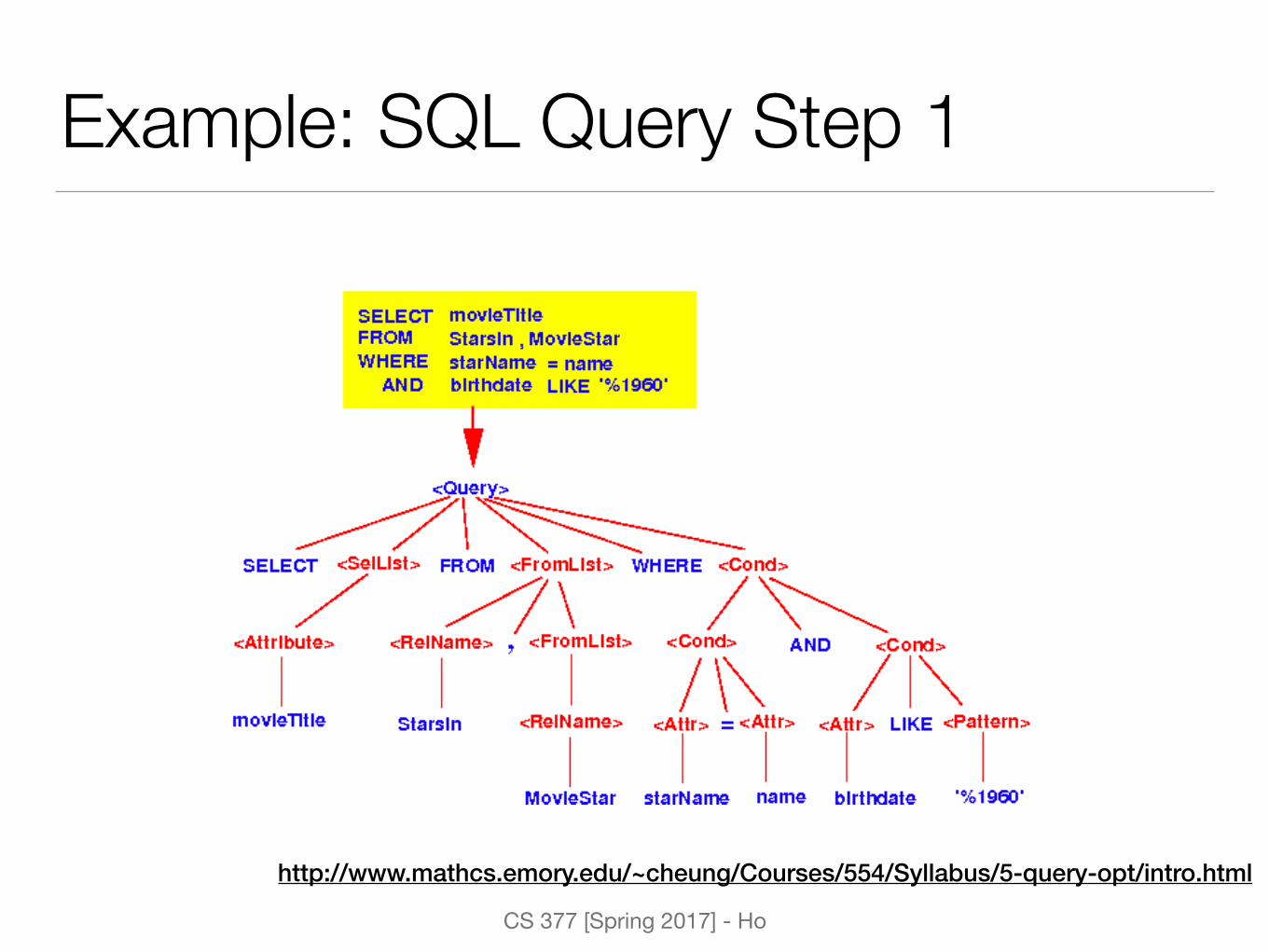
Example: SQL Query Step 1
http://www.mathcs.emory.edu/~cheung/Courses/554/Syllabus/5-query-opt/intro.html
CS 377 [Spring 2017] - Ho
Example: SQL Query Step 2
http://www.mathcs.emory.edu/~cheung/Courses/554/Syllabus/5-query-opt/intro.html

CS 377 [Spring 2017] - Ho
Example: SQL Query Step 3
http://www.mathcs.emory.edu/~cheung/Courses/554/Syllabus/5-query-opt/intro.html

CS 377 [Spring 2017] - Ho
Example: SQL Query Step 4
http://www.mathcs.emory.edu/~cheung/Courses/554/Syllabus/5-query-opt/intro.html
CS 377 [Spring 2017] - Ho
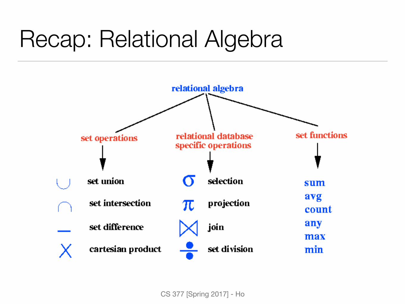
Recap: Relational Algebra
CS 377 [Spring 2017] - Ho
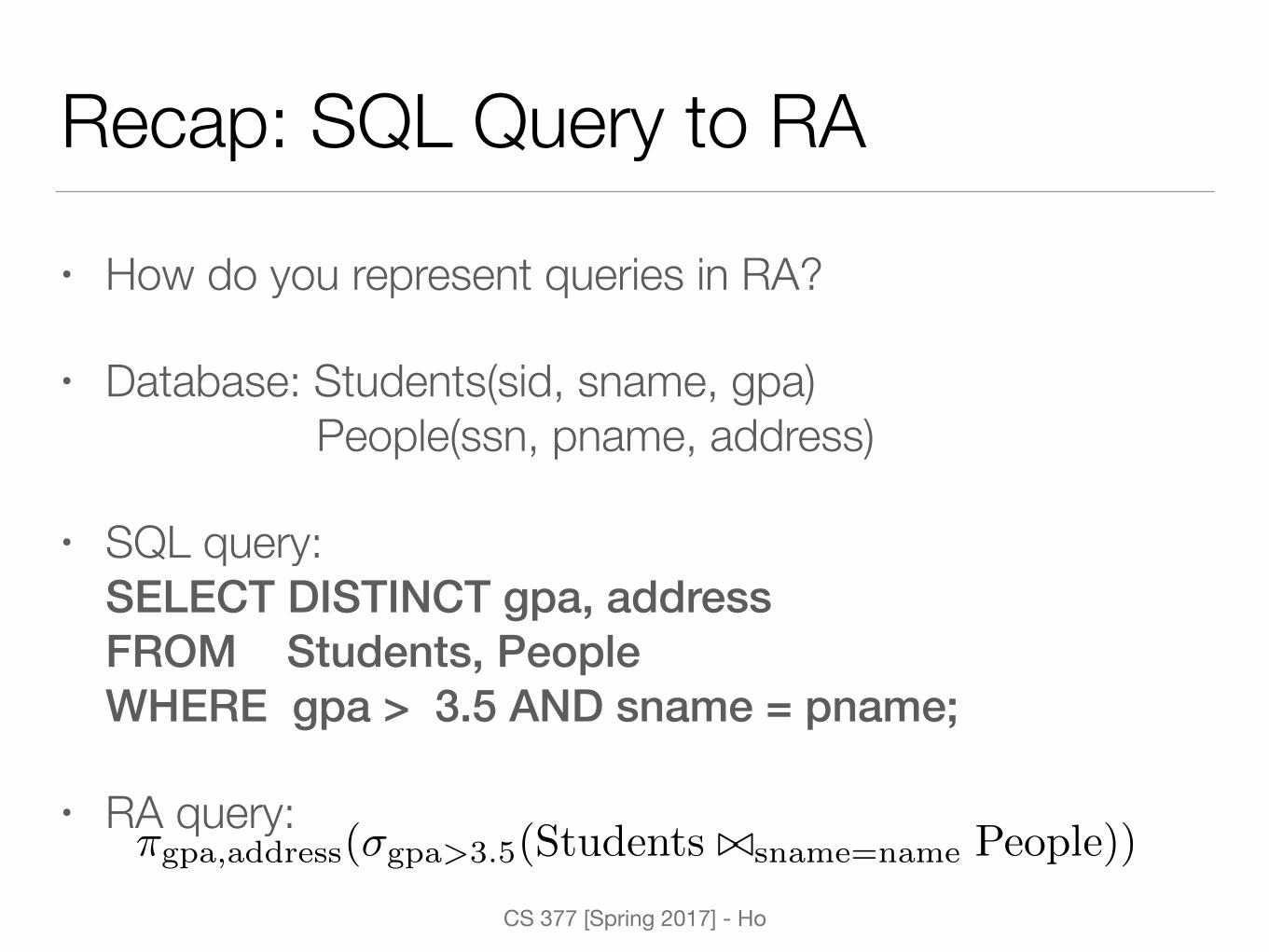
Recap: SQL Query to RA
• How do you represent queries in RA?
• Database: Students(sid, sname, gpa) People(ssn, pname, address)
• SQL query:SELECT DISTINCT gpa, address FROM Students, PeopleWHERE gpa > 3.5 AND sname = pname;
• RA query: ⇡gpa,address(�gpa>3.5(Students ./sname=name People))
CS 377 [Spring 2017] - Ho
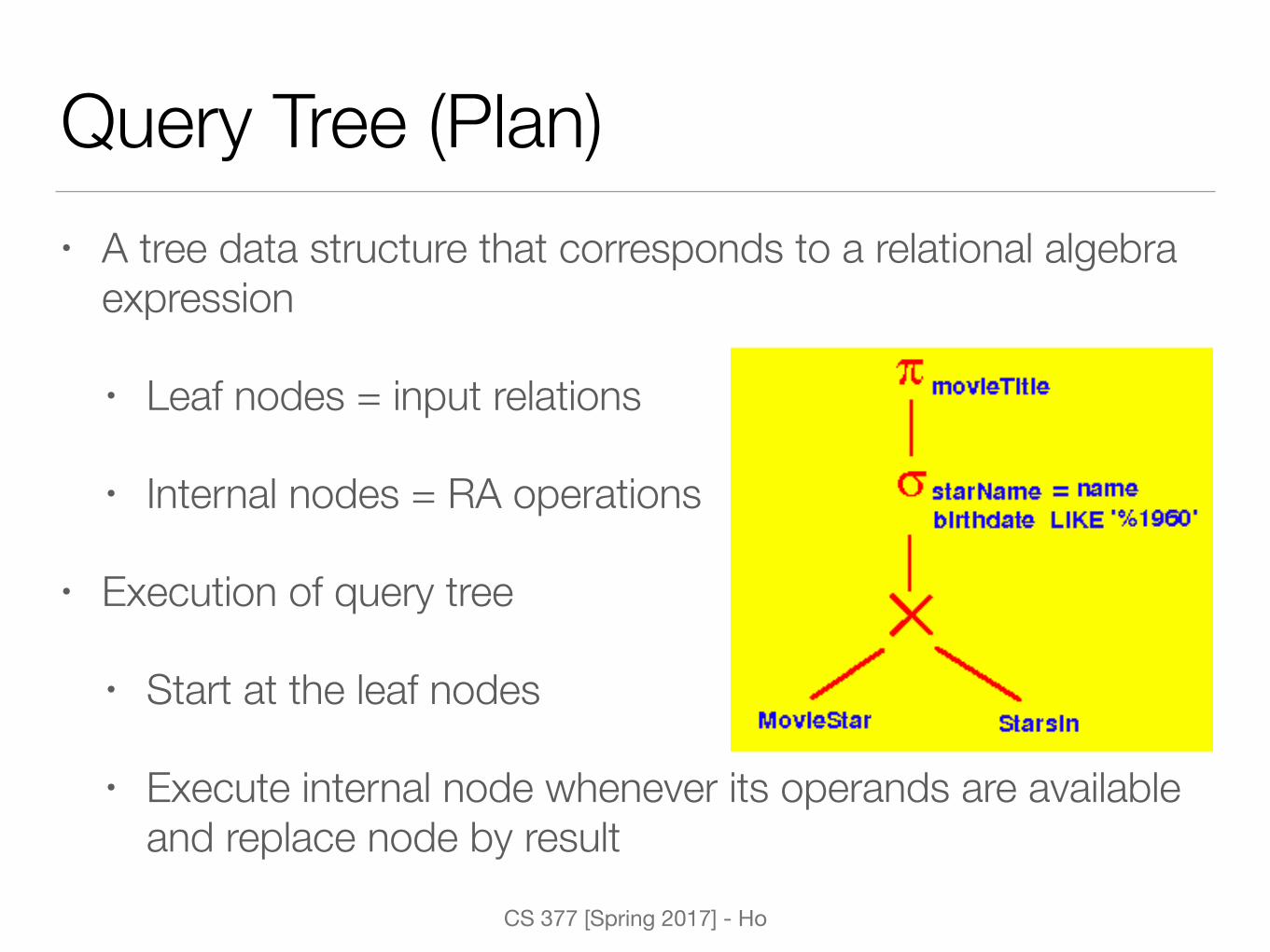
Query Tree (Plan)• A tree data structure that corresponds to a relational algebra
expression
• Leaf nodes = input relations
• Internal nodes = RA operations
• Execution of query tree
• Start at the leaf nodes
• Execute internal node whenever its operands are available and replace node by result
CS 377 [Spring 2017] - Ho
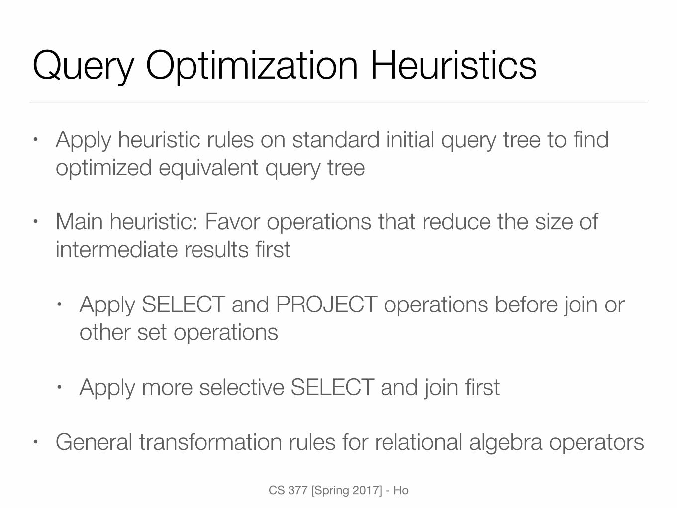
Query Optimization Heuristics• Apply heuristic rules on standard initial query tree to find
optimized equivalent query tree
• Main heuristic: Favor operations that reduce the size of intermediate results first
• Apply SELECT and PROJECT operations before join or other set operations
• Apply more selective SELECT and join first
• General transformation rules for relational algebra operators
CS 377 [Spring 2017] - Ho
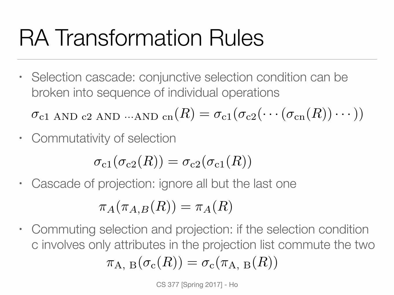
RA Transformation Rules• Selection cascade: conjunctive selection condition can be
broken into sequence of individual operations
• Commutativity of selection
• Cascade of projection: ignore all but the last one
• Commuting selection and projection: if the selection condition c involves only attributes in the projection list commute the two
�c1 AND c2 AND ···AND cn(R) = �c1(�c2(· · · (�cn(R)) · · · ))
�c1(�c2(R)) = �c2(�c1(R))
⇡A(⇡A,B(R)) = ⇡A(R)
⇡A, B(�c(R)) = �c(⇡A, B(R))

CS 377 [Spring 2017] - Ho
RA Transformation Rules• Commutativity of joins, cartesian product, union, intersection
• Associativity of join, cartesian product, union, intersection
• Selection and join: if attributes in the selection condition involves only attributes of one of the relations being joined
•
(R ✓ S) ✓ T = R ✓ (S ✓ T )
R ✓ S = S ✓ R
�c(R ./ S) = �c(R) ./ S
�c(R ./ S) = �c1(R) ./ �c2(S)
CS 377 [Spring 2017] - Ho
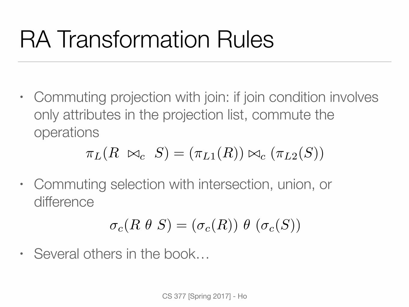
RA Transformation Rules
• Commuting projection with join: if join condition involves only attributes in the projection list, commute the operations
• Commuting selection with intersection, union, or difference
• Several others in the book…
�c(R ✓ S) = (�c(R)) ✓ (�c(S))
⇡L(R ./c S) = (⇡L1(R)) ./c (⇡L2(S))

CS 377 [Spring 2017] - Ho
Query Optimization Heuristic Algorithm
• Break up any select operations with conjunctive conditions into cascade of select operations and move select operations as far down query tree as permitted
• Rearrange leaf nodes so leaf nodes with most restrictive select operations are executed first
• Combine cartesian product operation with a subsequent selection operation into join operation

CS 377 [Spring 2017] - Ho
Query Optimization Heuristic Algorithm
• Break down and move lists of projection attributes down the tree as far as possible
• Identify subtrees that represent group of operations that can be executed as a single algorithm

CS 377 [Spring 2017] - Ho
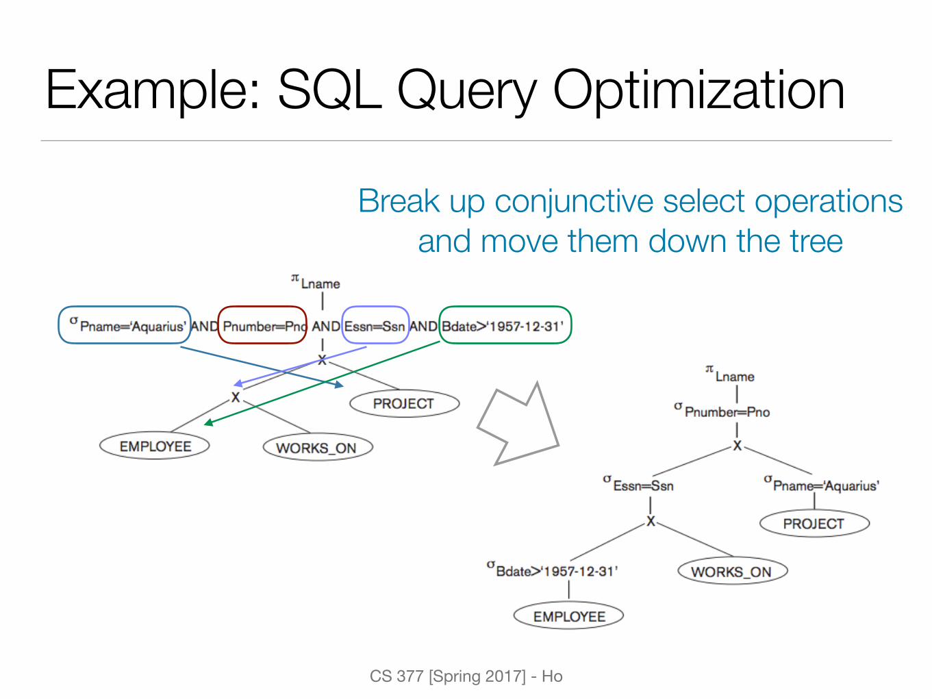
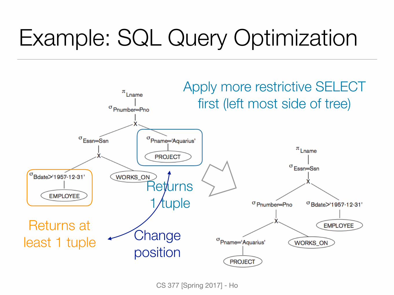
Example: SQL Query OptimizationSELECT lname FROM employee, works_on, project WHERE pname = ‘Aquarius’ and pnumber = pno AND bdate > ‘1957-12-31’;
Initial query tree
CS 377 [Spring 2017] - Ho
Example: SQL Query Optimization
Break up conjunctive select operations and move them down the tree
CS 377 [Spring 2017] - Ho
Example: SQL Query Optimization
Returns 1 tuple
Returns at least 1 tuple Change
position
Apply more restrictive SELECT first (left most side of tree)

CS 377 [Spring 2017] - Ho
Example: SQL Query Optimization
Replace cartesian product and select with join
CS 377 [Spring 2017] - Ho
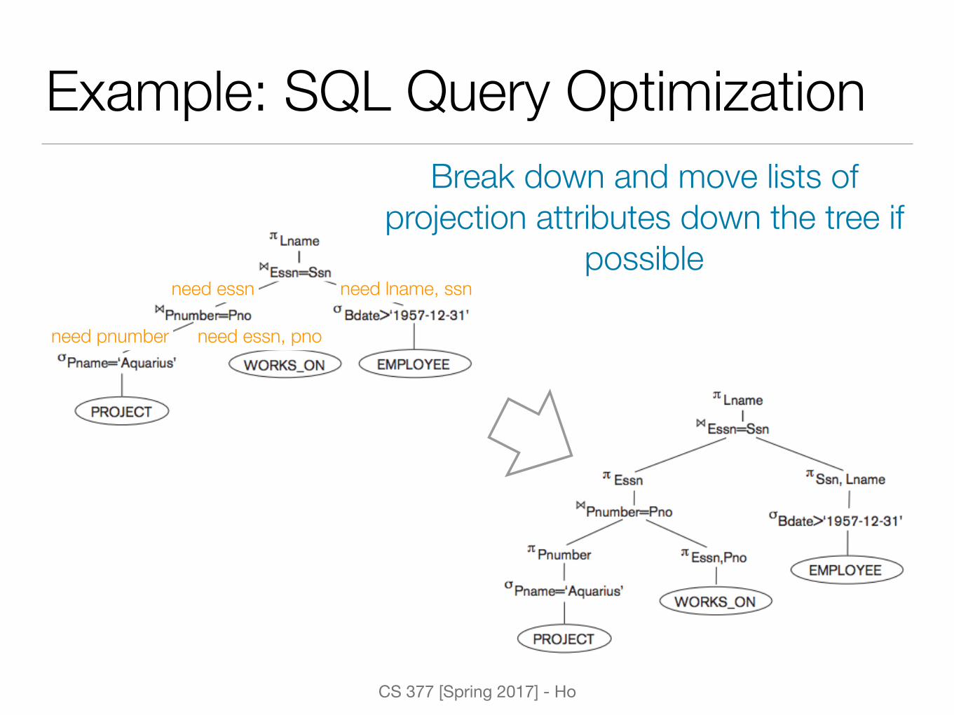
Example: SQL Query OptimizationBreak down and move lists of
projection attributes down the tree if possible
need lname, ssnneed essn
need essn, pnoneed pnumber
CS 377 [Spring 2017] - Ho
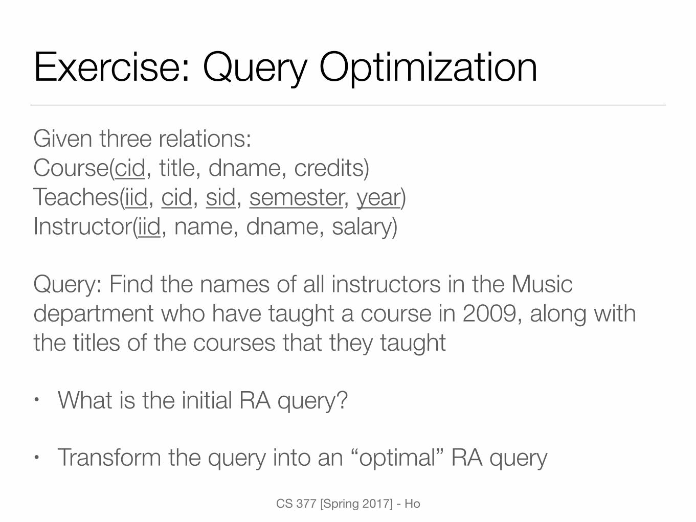
Exercise: Query OptimizationGiven three relations: Course(cid, title, dname, credits)Teaches(iid, cid, sid, semester, year) Instructor(iid, name, dname, salary)
Query: Find the names of all instructors in the Music department who have taught a course in 2009, along with the titles of the courses that they taught
• What is the initial RA query?
• Transform the query into an “optimal” RA query
CS 377 [Spring 2017] - Ho
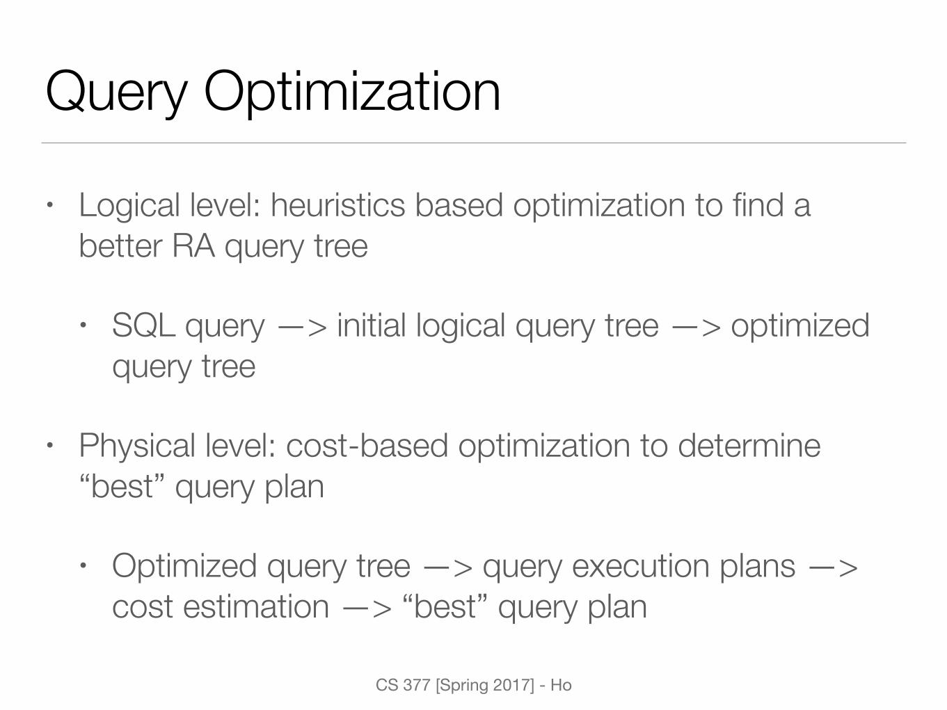
Query Optimization
• Logical level: heuristics based optimization to find a better RA query tree
• SQL query —> initial logical query tree —> optimized query tree
• Physical level: cost-based optimization to determine “best” query plan
• Optimized query tree —> query execution plans —> cost estimation —> “best” query plan
CS 377 [Spring 2017] - Ho
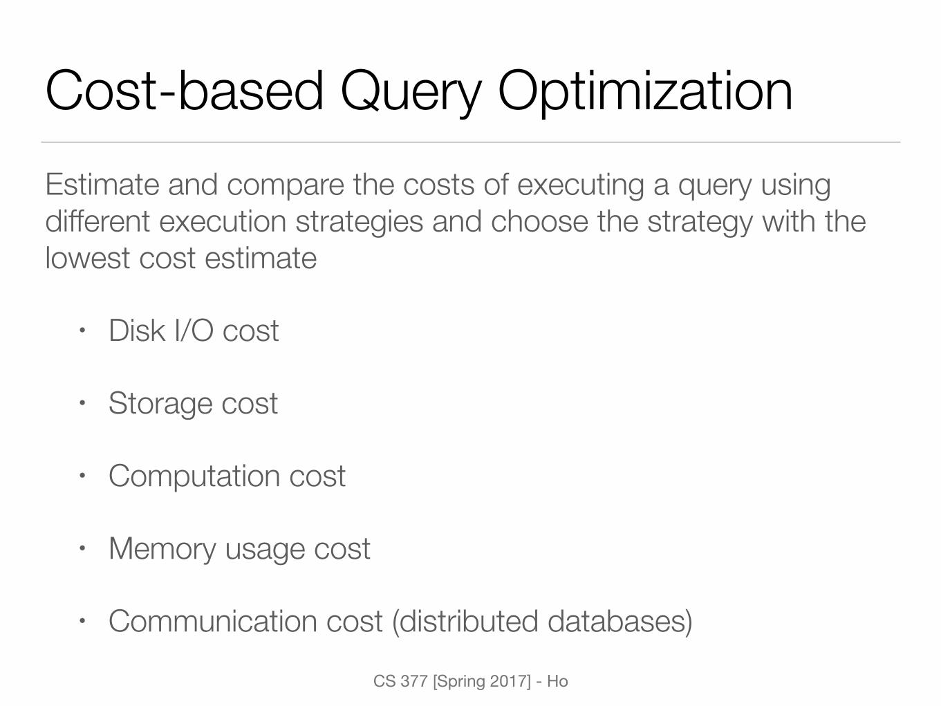
Cost-based Query OptimizationEstimate and compare the costs of executing a query using different execution strategies and choose the strategy with the lowest cost estimate
• Disk I/O cost
• Storage cost
• Computation cost
• Memory usage cost
• Communication cost (distributed databases)

CS 377 [Spring 2017] - Ho
Catalog InformationDatabase maintains statistics about each relation
• Size of file: number of tuples [nr], number of blocks [br], tuple size [sr], number of tuples or records per block [fr], etc.
• Information about indexes and indexing attributes
• Attribute values - number of distinct values [V(att, r)]
• Selection cardinality - expected size of selection given value [SC(att, r)]
• …

CS 377 [Spring 2017] - Ho
Catalog Information for Index
• Average fan-out of internal nodes of index i for tree-structured indices [fi]
• Number of levels in index i (i.e., height of index i) [HTi]
• Balanced tree on attribute A of relation r:
• Hash index: 1
• Number of lowest-level index blocks in i (i.e., number of blocks at the leaf level of the index) [LBi]
dlogfi V (A, r)e

CS 377 [Spring 2017] - Ho
Example: Bank SchemaAccount relation
• faccount = 20 (20 tuples per block)
• V(bname, account) = 50 (50 branches)
• V(balance, account) = 500 (500 different balance values)
• naccount = 10000 (10,000 tuples in account)
• baccount = 10000 / 20 = 500
CS 377 [Spring 2017] - Ho
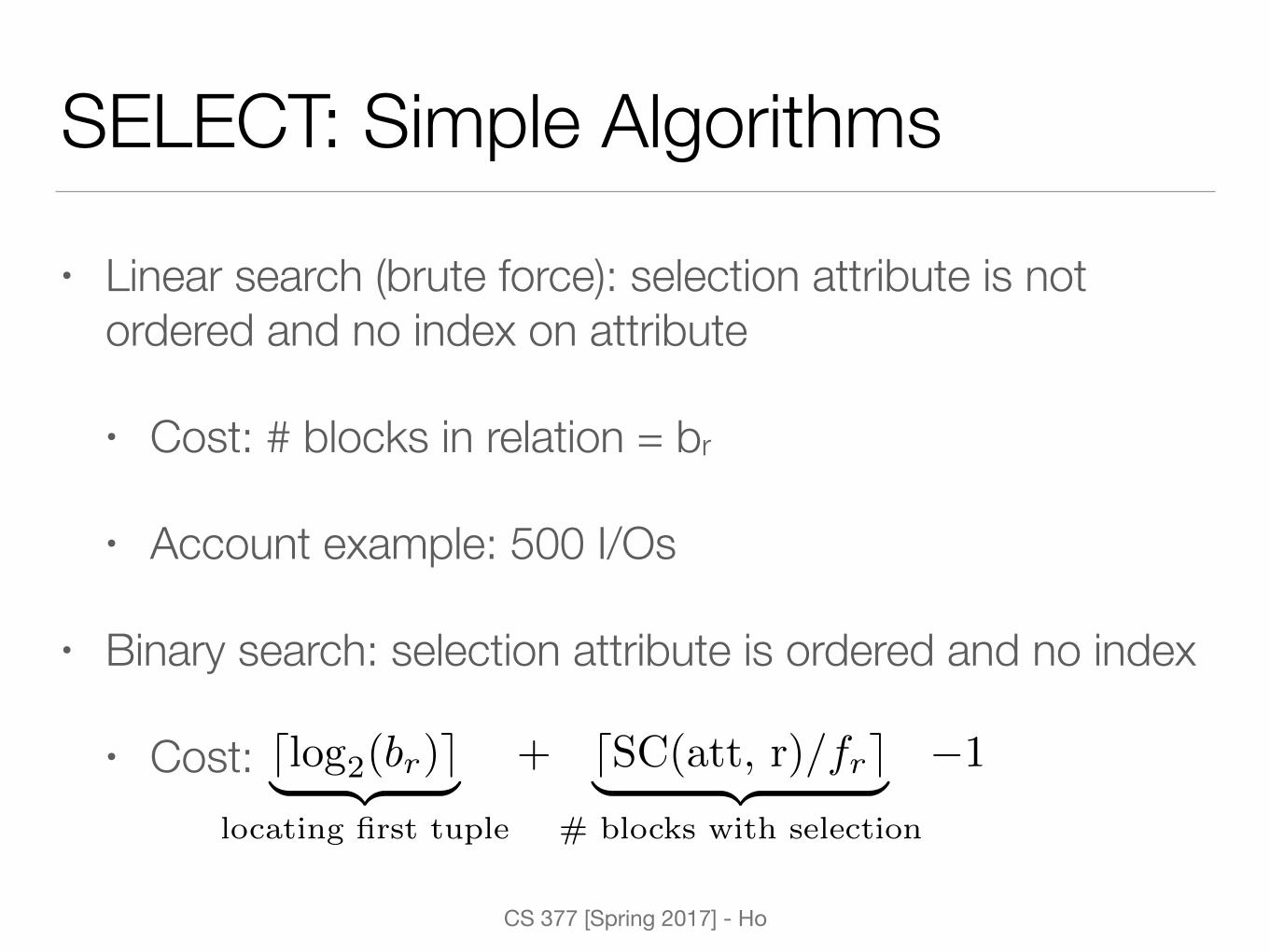
SELECT: Simple Algorithms
• Linear search (brute force): selection attribute is not ordered and no index on attribute
• Cost: # blocks in relation = br
• Account example: 500 I/Os
• Binary search: selection attribute is ordered and no index
• Cost:
dlog2
(br)e| {z }locating first tuple
+ dSC(att, r)/fre| {z }# blocks with selection
�1
CS 377 [Spring 2017] - Ho
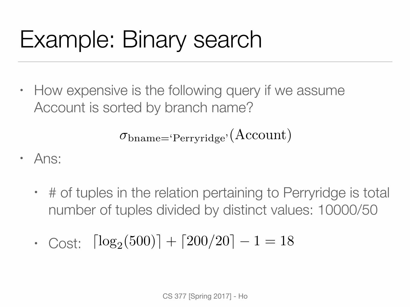
Example: Binary search
• How expensive is the following query if we assume Account is sorted by branch name?
• Ans:
• # of tuples in the relation pertaining to Perryridge is total number of tuples divided by distinct values: 10000/50
• Cost:
�bname=‘Perryridge’(Account)
dlog2(500)e+ d200/20e � 1 = 18

CS 377 [Spring 2017] - Ho
SELECT: Simple Algorithm with Index
• Index search: cost depends on the number of qualifying tuples, cost of retrieving the tuples and the type of query
• Primary index
• Equality search on candidate key:
• Equality search on nonkey:
• Comparison search: estimated number of tuples that satisfy condition
HTi + dSC(att, r)/fre
HTi + 1
HTi + dc/fre
CS 377 [Spring 2017] - Ho
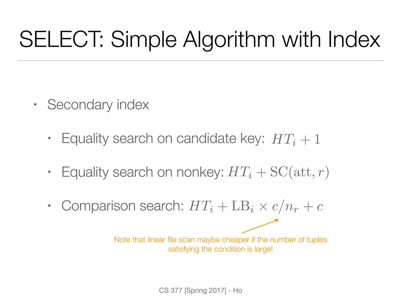
SELECT: Simple Algorithm with Index
• Secondary index
• Equality search on candidate key:
• Equality search on nonkey:
• Comparison search:
Note that linear file scan maybe cheaper if the number of tuples satisfying the condition is large!
HTi + 1
HTi + SC(att, r)
HTi + LBi ⇥ c/nr + c
CS 377 [Spring 2017] - Ho
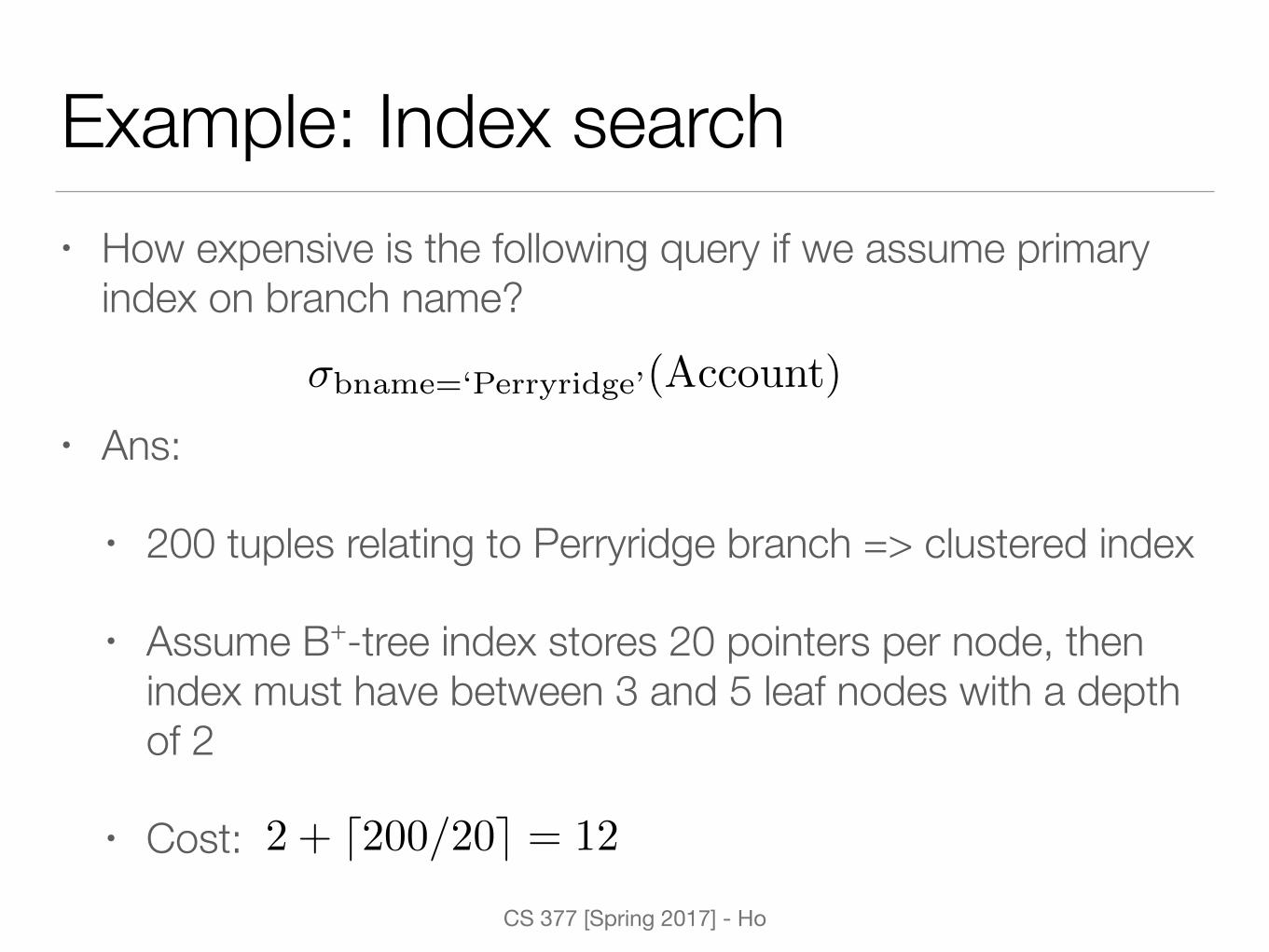
Example: Index search• How expensive is the following query if we assume primary
index on branch name?
• Ans:
• 200 tuples relating to Perryridge branch => clustered index
• Assume B+-tree index stores 20 pointers per node, then index must have between 3 and 5 leaf nodes with a depth of 2
• Cost:
�bname=‘Perryridge’(Account)
2 + d200/20e = 12
CS 377 [Spring 2017] - Ho
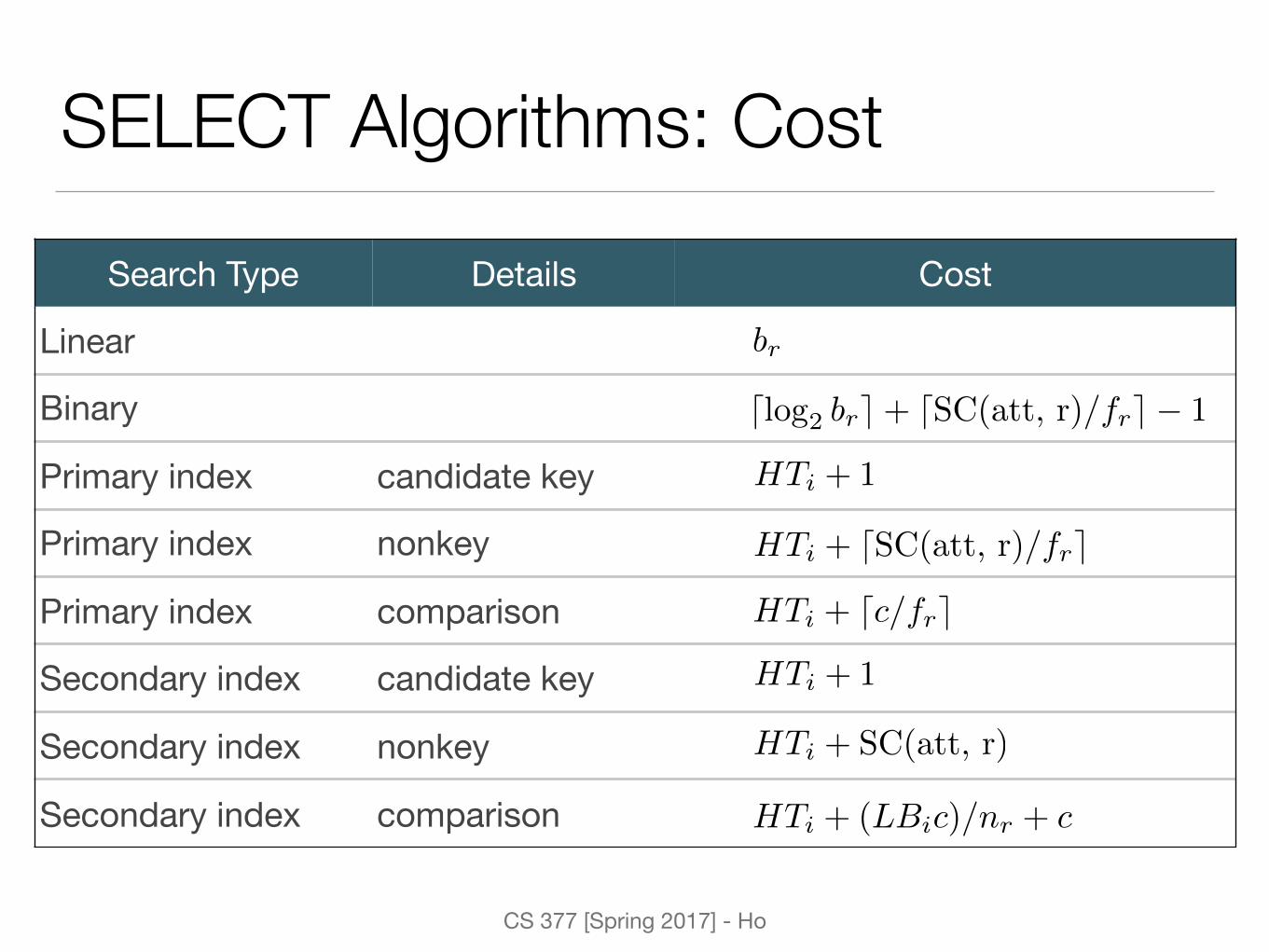
Search Type Details Cost
Linear
Binary
Primary index candidate key
Primary index nonkey
Primary index comparison
Secondary index candidate key
Secondary index nonkey
Secondary index comparison
SELECT Algorithms: Cost
dlog2 bre+ dSC(att, r)/fre � 1
br
HTi + 1
HTi + 1
HTi + dSC(att, r)/fre
HTi + SC(att, r)
HTi + dc/fre
HTi + (LBic)/nr + c

CS 377 [Spring 2017] - Ho
Exercise: SELECT• Employee relation with clustering index on salary:
• nemployee = 10,000 (10,000 tuples in employee)
• bemployee = 2,000 (2,000 blocks)
• Secondary index (B+-Tree) on SSN (key attribute)
• HTi = 4 levels
• What algorithm would be used for the following query and why? �SSN=123456789(Employee)
CS 377 [Spring 2017] - Ho
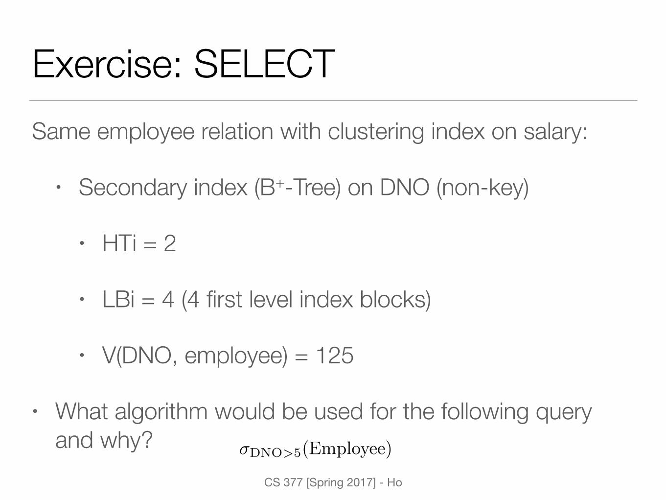
Exercise: SELECTSame employee relation with clustering index on salary:
• Secondary index (B+-Tree) on DNO (non-key)
• HTi = 2
• LBi = 4 (4 first level index blocks)
• V(DNO, employee) = 125
• What algorithm would be used for the following query and why? �DNO>5(Employee)

CS 377 [Spring 2017] - Ho
SELECT: Complex Algorithms• Conjunctive selection (several conditions with AND)
• Single index: retrieve records satisfying some attribute condition (with index) and check remaining conditions
• Composite index
• Intersection of multiple indexes
• Disjunctive selection (several conditions with OR)
• Index/binary search if all conditions have access path and take union
• Linear search otherwise

CS 377 [Spring 2017] - Ho
Example: Complex search• How expensive if we want to find accounts where the branch name
is Perryridge with a balance of 1200 if we assume there is a primary index on branch name and secondary on balance?
• Ans for using one index:
• Cost for branch name: 12 block reads
• Balance index is not clustered, so expected selection is 10,000 / 500 = 20 accounts
• Cost for balance: 2 + 20 = 22 block reads
• Thus use branch name index, even if it is less selective!

CS 377 [Spring 2017] - Ho
Example: Complex search• Ans for using intersection of two indexes:
• Use index on balance to retrieve set of S1 pointers: 2 reads
• Use index on branch name to retrieve set of S2 pointers: 2 reads
• Take intersection of the two
• Estimate 1 tuple in 50 * 500 meets both conditions, so we estimate the intersection of two has one pointer
• Estimated cost: 5 block reads

CS 377 [Spring 2017] - Ho
Sorting• One of the primary algorithms used for query processing
• ORDER BY
• DISTINCT
• JOIN
• Relations that fit in memory — use techniques like quicksort, merge sort, bubble sort
• Relations that don’t fit in memory — external sort-merge
CS 377 [Spring 2017] - Ho
JOIN
• One of the most time-consuming operations
• EQUIJOIN & NATURAL JOIN varieties are most prominent — focus on algorithms for these
• Two way join: join on two files
• Multi-way joins: joins involving more than two files
CS 377 [Spring 2017] - Ho
JOIN Performance
Factors that affect performance
• Tuples of relation stored physically together
• Relations sorted by join attribute
• Existence of indexes
CS 377 [Spring 2017] - Ho
JOIN Algorithms• Several different algorithms to implement joins
• Nested loop join
• Nested-block join
• Indexed nested loop join
• Sort-merge join
• Hash-join
• Choice is based on cost estimate

CS 377 [Spring 2017] - Ho
Example: Bank Schema• Join depositor and customer tables
• Catalog information for both relations:
• ncustomer = 10000
• fcustomer = 25 => bcustomer = 10000/25 = 400
• ndepositor = 5000
• fdepositor = 50 => bdepositor = 5000/50 = 100
• V(cname, depositor) = 2500 (each customer on average has 2 accounts)
• Cname in depositor is a foreign key of customer
CS 377 [Spring 2017] - Ho
Cardinality of Join Queries
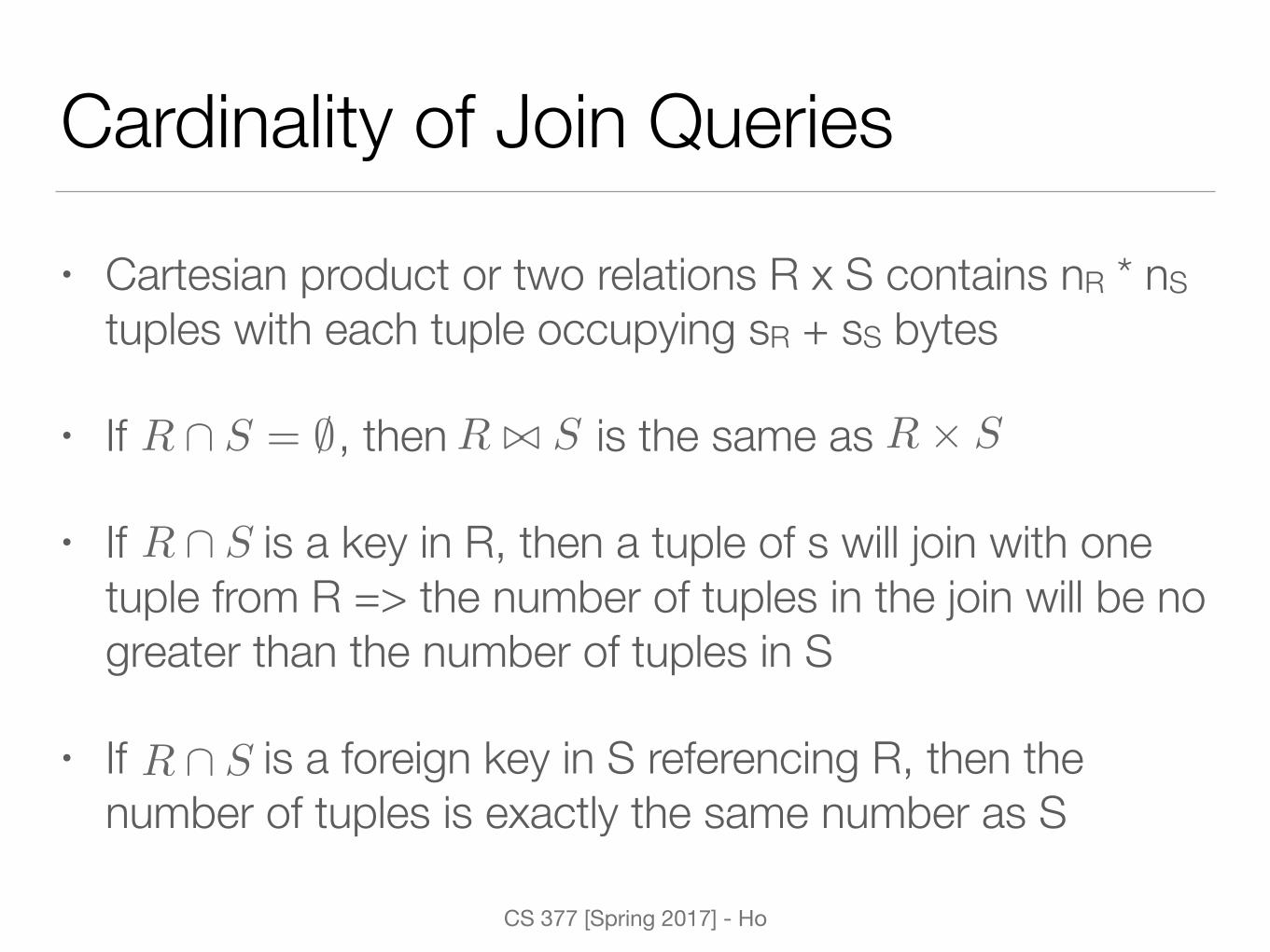
• Cartesian product or two relations R x S contains nR * nS tuples with each tuple occupying sR + sS bytes
• If , then is the same as
• If is a key in R, then a tuple of s will join with one tuple from R => the number of tuples in the join will be no greater than the number of tuples in S
• If is a foreign key in S referencing R, then the number of tuples is exactly the same number as S
R \ S = ; R ./ S R⇥ S
R \ S
R \ S
CS 377 [Spring 2017] - Ho
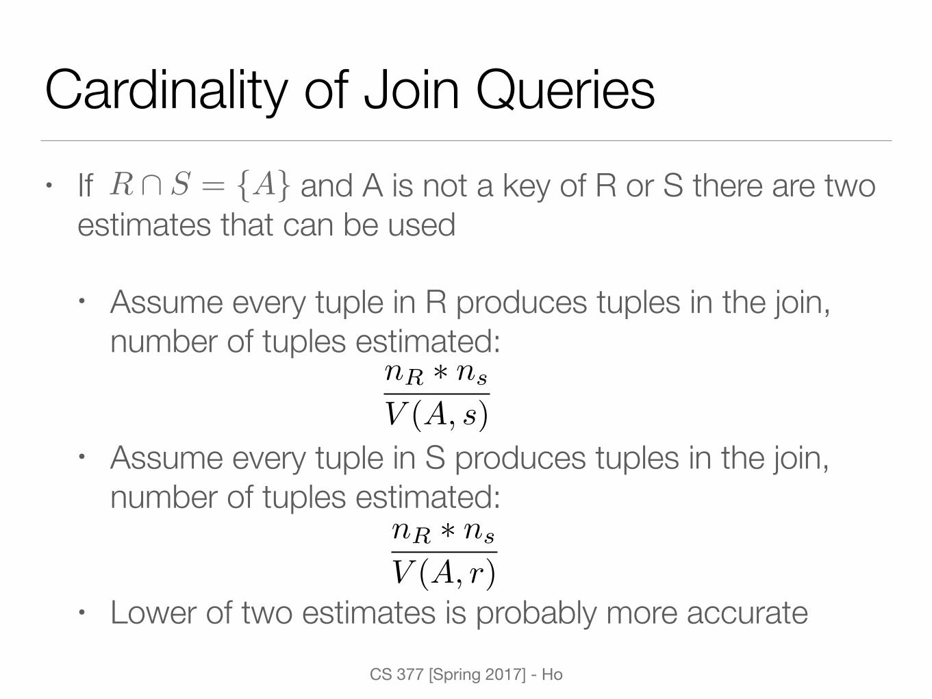
Cardinality of Join Queries• If and A is not a key of R or S there are two
estimates that can be used
• Assume every tuple in R produces tuples in the join, number of tuples estimated:
• Assume every tuple in S produces tuples in the join, number of tuples estimated:
• Lower of two estimates is probably more accurate
R \ S = {A}
nR ⇤ ns
V (A, s)
nR ⇤ ns
V (A, r)
CS 377 [Spring 2017] - Ho
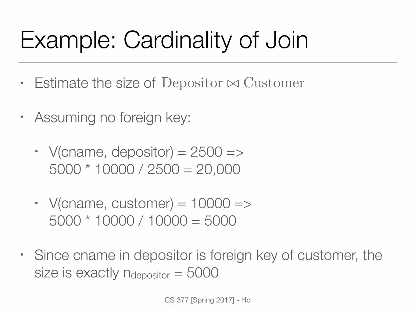
Example: Cardinality of Join• Estimate the size of
• Assuming no foreign key:
• V(cname, depositor) = 2500 => 5000 * 10000 / 2500 = 20,000
• V(cname, customer) = 10000 =>5000 * 10000 / 10000 = 5000
• Since cname in depositor is foreign key of customer, the size is exactly ndepositor = 5000
Depositor ./ Customer
CS 377 [Spring 2017] - Ho
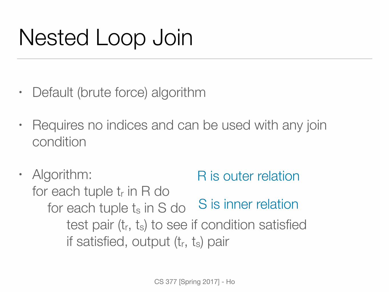
Nested Loop Join
• Default (brute force) algorithm
• Requires no indices and can be used with any join condition
• Algorithm: for each tuple tr in R do for each tuple ts in S do test pair (tr, ts) to see if condition satisfied if satisfied, output (tr, ts) pair
R is outer relation
S is inner relation

CS 377 [Spring 2017] - Ho
Nested Loop Join Cost
• Algorithm: for each tuple tr in R do for each tuple ts in S do test pair (tr, ts) to see if condition satisfied if satisfied, output (tr, ts) pair
Read in tuples of R: brFor every tuple in R read S: bs
Worst case: br + nr x bs

CS 377 [Spring 2017] - Ho
Nested Loop Join Cost
• Algorithm: for each tuple tr in R do for each tuple ts in S do test pair (tr, ts) to see if condition satisfied if satisfied, output (tr, ts) pair
Read in tuples of R: brFor every tuple in R read S: bs
If smaller block fits into memory, we can avoid the cost of re-reading relation S — cost = br + bs
CS 377 [Spring 2017] - Ho
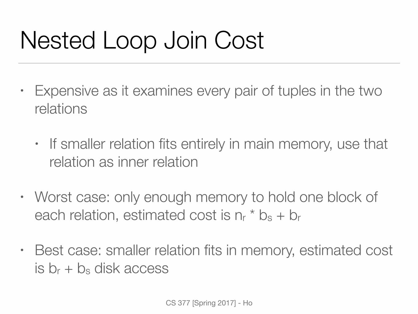
Nested Loop Join Cost
• Expensive as it examines every pair of tuples in the two relations
• If smaller relation fits entirely in main memory, use that relation as inner relation
• Worst case: only enough memory to hold one block of each relation, estimated cost is nr * bs + br
• Best case: smaller relation fits in memory, estimated cost is br + bs disk access
CS 377 [Spring 2017] - Ho
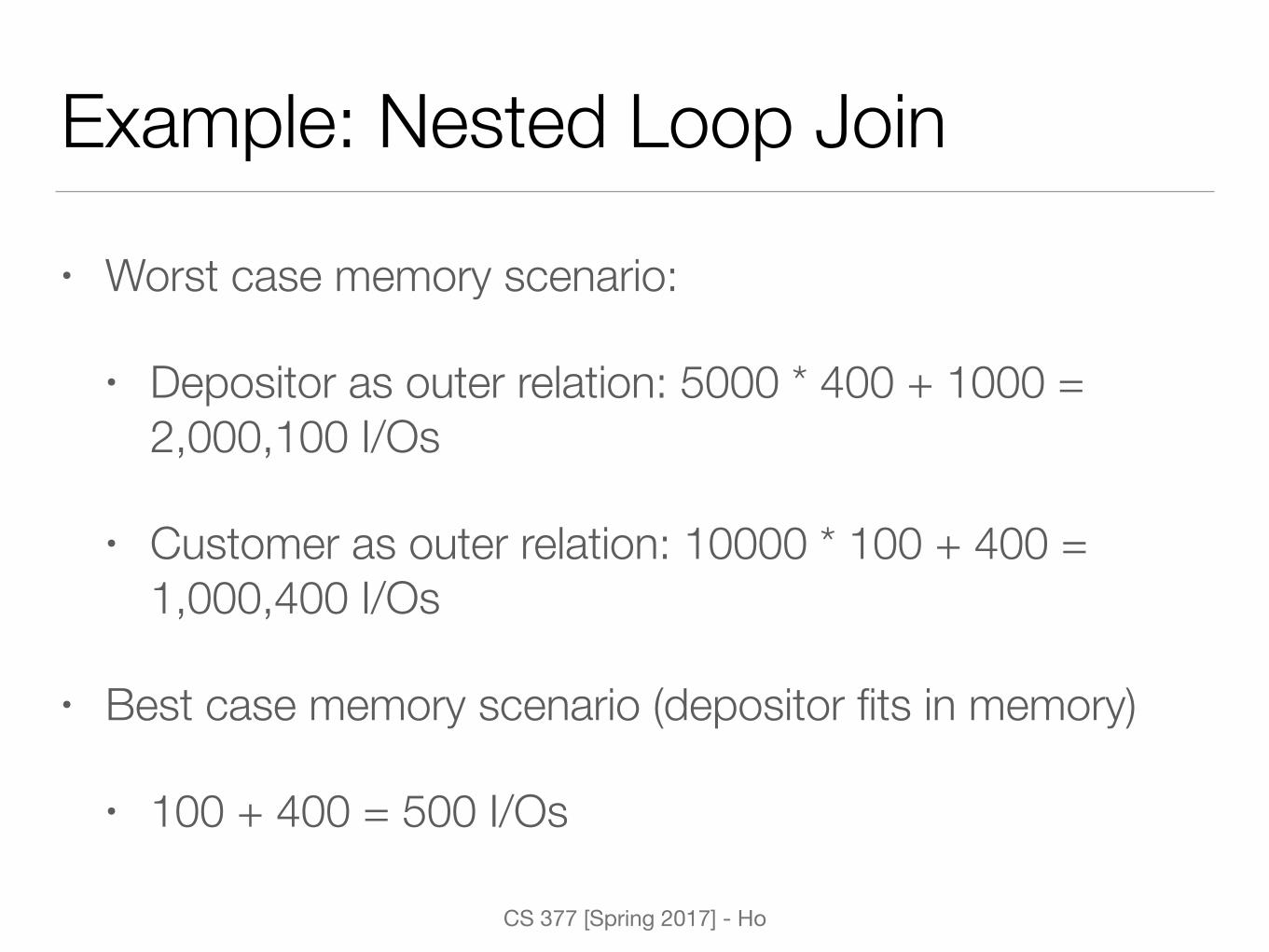
Example: Nested Loop Join
• Worst case memory scenario:
• Depositor as outer relation: 5000 * 400 + 1000 = 2,000,100 I/Os
• Customer as outer relation: 10000 * 100 + 400 = 1,000,400 I/Os
• Best case memory scenario (depositor fits in memory)
• 100 + 400 = 500 I/Os
CS 377 [Spring 2017] - Ho
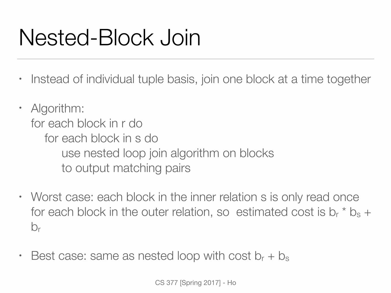
Nested-Block Join• Instead of individual tuple basis, join one block at a time together
• Algorithm:for each block in r do for each block in s do use nested loop join algorithm on blocks to output matching pairs
• Worst case: each block in the inner relation s is only read once for each block in the outer relation, so estimated cost is br * bs + br
• Best case: same as nested loop with cost br + bs
CS 377 [Spring 2017] - Ho
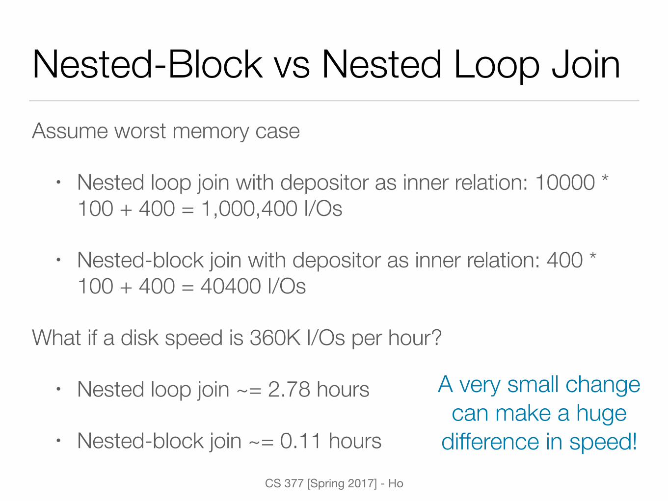
Nested-Block vs Nested Loop JoinAssume worst memory case
• Nested loop join with depositor as inner relation: 10000 * 100 + 400 = 1,000,400 I/Os
• Nested-block join with depositor as inner relation: 400 * 100 + 400 = 40400 I/Os
What if a disk speed is 360K I/Os per hour?
• Nested loop join ~= 2.78 hours
• Nested-block join ~= 0.11 hours
A very small change can make a huge
difference in speed!
CS 377 [Spring 2017] - Ho
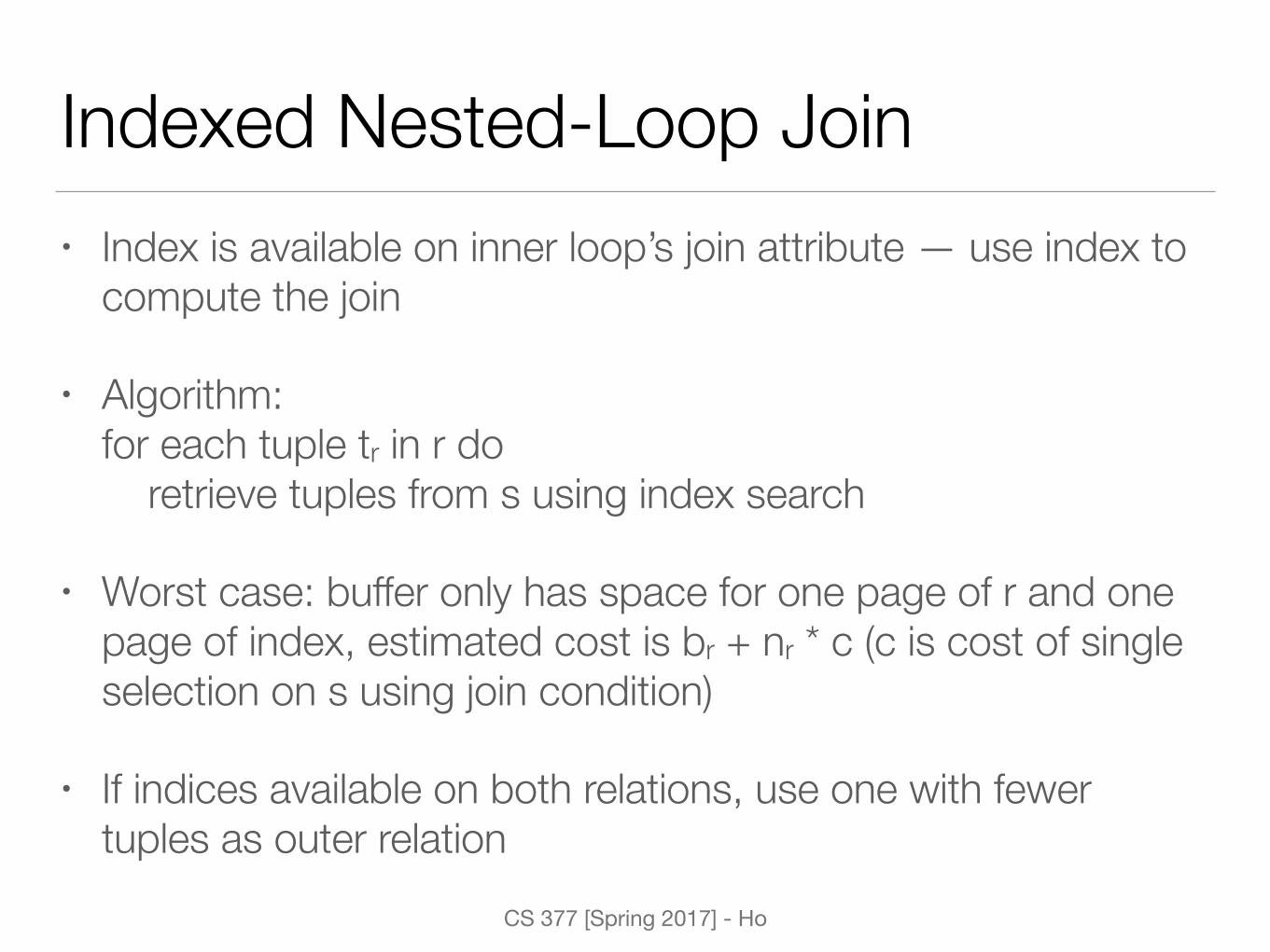
Indexed Nested-Loop Join• Index is available on inner loop’s join attribute — use index to
compute the join
• Algorithm: for each tuple tr in r do retrieve tuples from s using index search
• Worst case: buffer only has space for one page of r and one page of index, estimated cost is br + nr * c (c is cost of single selection on s using join condition)
• If indices available on both relations, use one with fewer tuples as outer relation
CS 377 [Spring 2017] - Ho
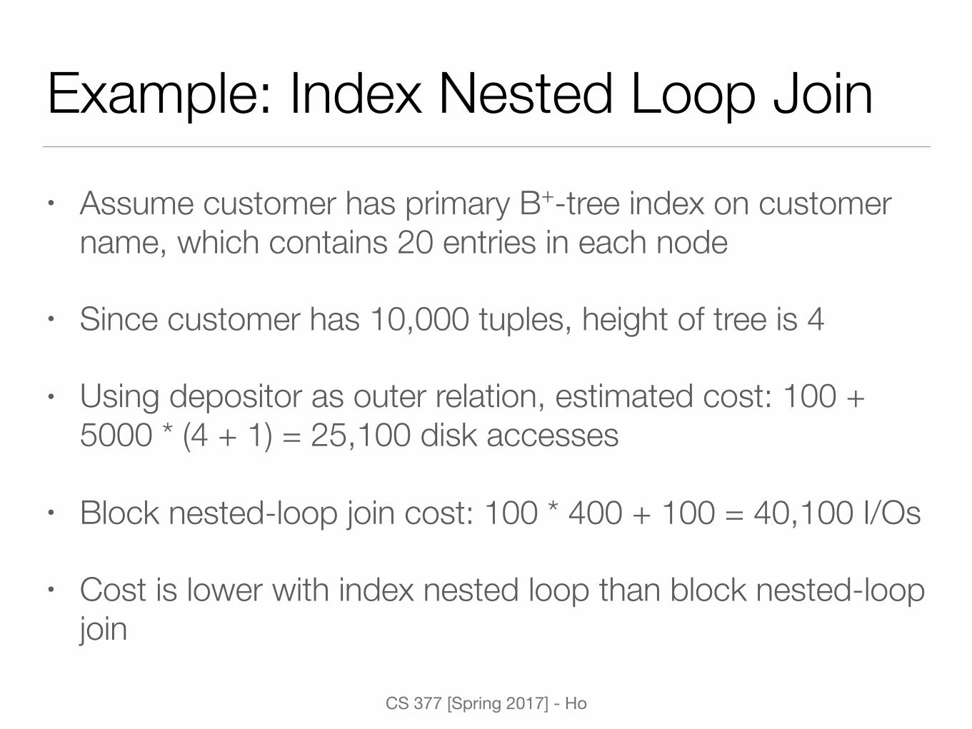
Example: Index Nested Loop Join• Assume customer has primary B+-tree index on customer
name, which contains 20 entries in each node
• Since customer has 10,000 tuples, height of tree is 4
• Using depositor as outer relation, estimated cost: 100 + 5000 * (4 + 1) = 25,100 disk accesses
• Block nested-loop join cost: 100 * 400 + 100 = 40,100 I/Os
• Cost is lower with index nested loop than block nested-loop join
a 3b 1d 8
13df 7
m 5q 6
a Ab Gc Ld Nm B
a1 a2 a1 a3pr ps
r
s
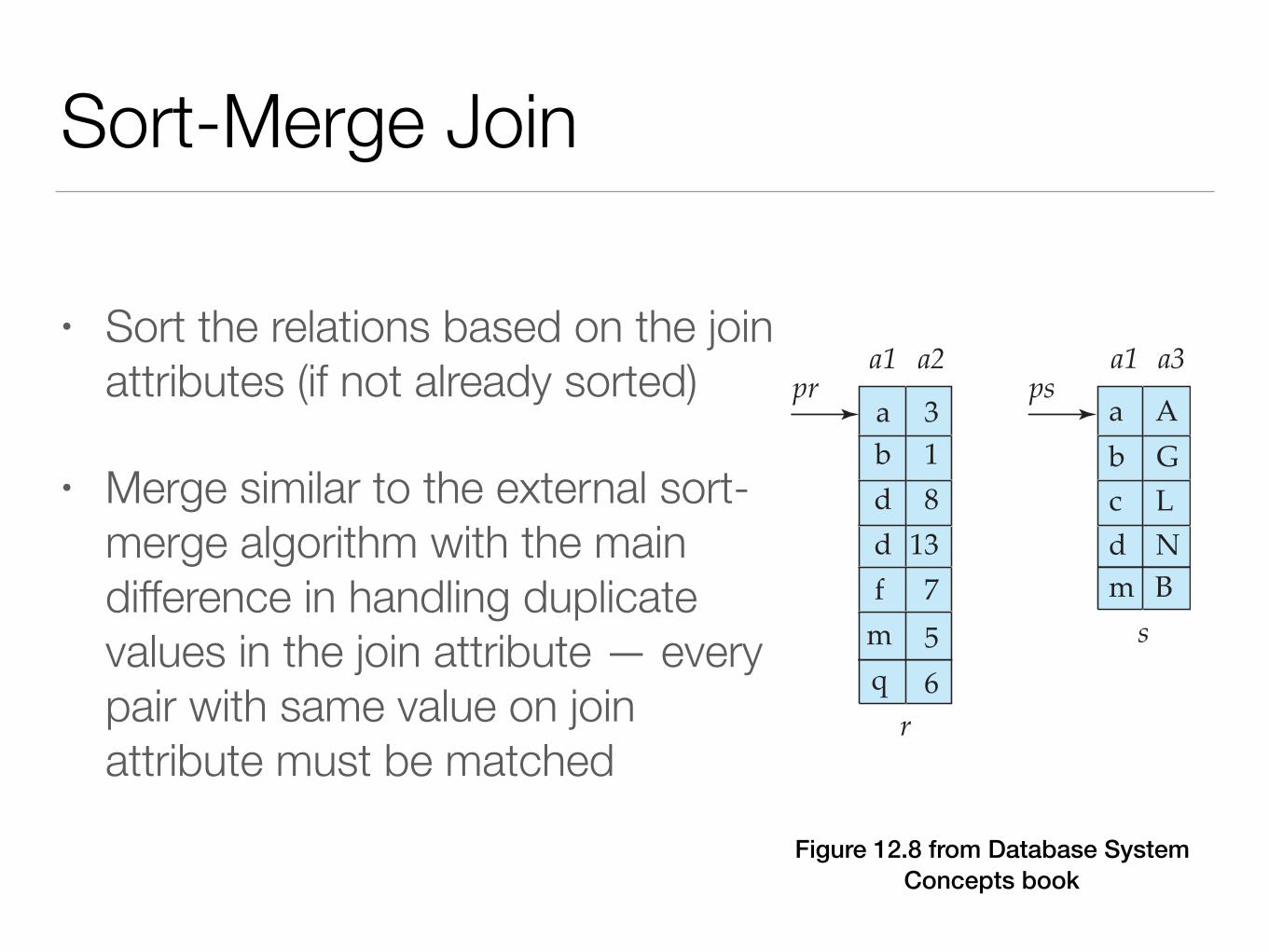
Sort-Merge Join
• Sort the relations based on the join attributes (if not already sorted)
• Merge similar to the external sort-merge algorithm with the main difference in handling duplicate values in the join attribute — every pair with same value on join attribute must be matched
Figure 12.8 from Database System Concepts book

CS 377 [Spring 2017] - Ho
Sort-Merge Join
• Can only be used for equijoins and natural joins
• Each tuple needs to be read only once, and as a result, each block is also read only once cost = sorting cost + br + bs
• If one relation is sorted, and other has secondary B+-tree index on join attribute, hybrid merge-joins are possible

ga d 31c 33b 14e 16r 16d 21m 3p 2d 7a 14
a 14a 19b 14c 33d 7d 21d 31e 16g 24m 3p 2r 16
a 19b 14c 33d 31e 16g 24
a 14d 7d 21m 3p 2r 16
a 19d 31g 24
b 14c 33e 16
d 21m 3r 16
a 14d 7p 2
initialrelation
createruns
mergepass–1
mergepass–2
runs runssortedoutput
2419
External Sort Merge Algorithm
• Sort r records, stored in b file blocks with a total memory space of M blocks (relation is larger than memory)
• Total cost:
Figure 12.4 from Database System Concepts book
2br(dlogM�1(br/M)e+ 1)
NOTE: that the previous slides were off by a factor of 2 for the second part!
CS 377 [Spring 2017] - Ho
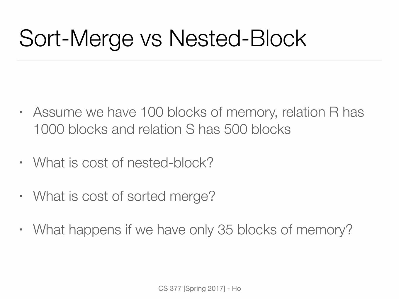
Sort-Merge vs Nested-Block
• Assume we have 100 blocks of memory, relation R has 1000 blocks and relation S has 500 blocks
• What is cost of nested-block?
• What is cost of sorted merge?
• What happens if we have only 35 blocks of memory?

CS 377 [Spring 2017] - Ho
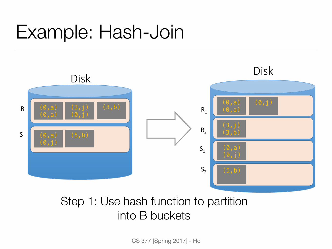
Hash-Join
• Applicable for equijoins and natural joins
• A hash function, h, is used to partition tuples of both relations into sets that have same hash value on the join attributes
• Tuples in the corresponding same buckets just need to be compared with one another and not with all the other tuples in the other buckets
CS 377 [Spring 2017] - Ho
Example: Hash-Join
Disk
R
S
(3,j) !(0,j) !
(0,a) !(0,a) !
(3,b) !!
(5,b) !!
(0,a) !(0,j) !
Disk
R1
S1
S2
R2
(0,a) !(0,a) !
(0,j) !!
(3,j) !(3,b) !
(0,a) !(0,j) !
(5,b) !!
(5,b) !!
Step 1: Use hash function to partition into B buckets

CS 377 [Spring 2017] - Ho
Example: Hash-Join
Disk
R
S
(3,j) !(0,j) !
(0,a) !(0,a) !
(3,b) !!
(5,b) !!
(0,a) !(0,j) !
Disk
R1
S1
S2
R2
(0,a) !(0,a) !
(0,j) !!
(3,j) !(3,b) !
(0,a) !(0,j) !
(5,b) !!
(5,b) !!
Step 2: Join matching buckets
CS 377 [Spring 2017] - Ho
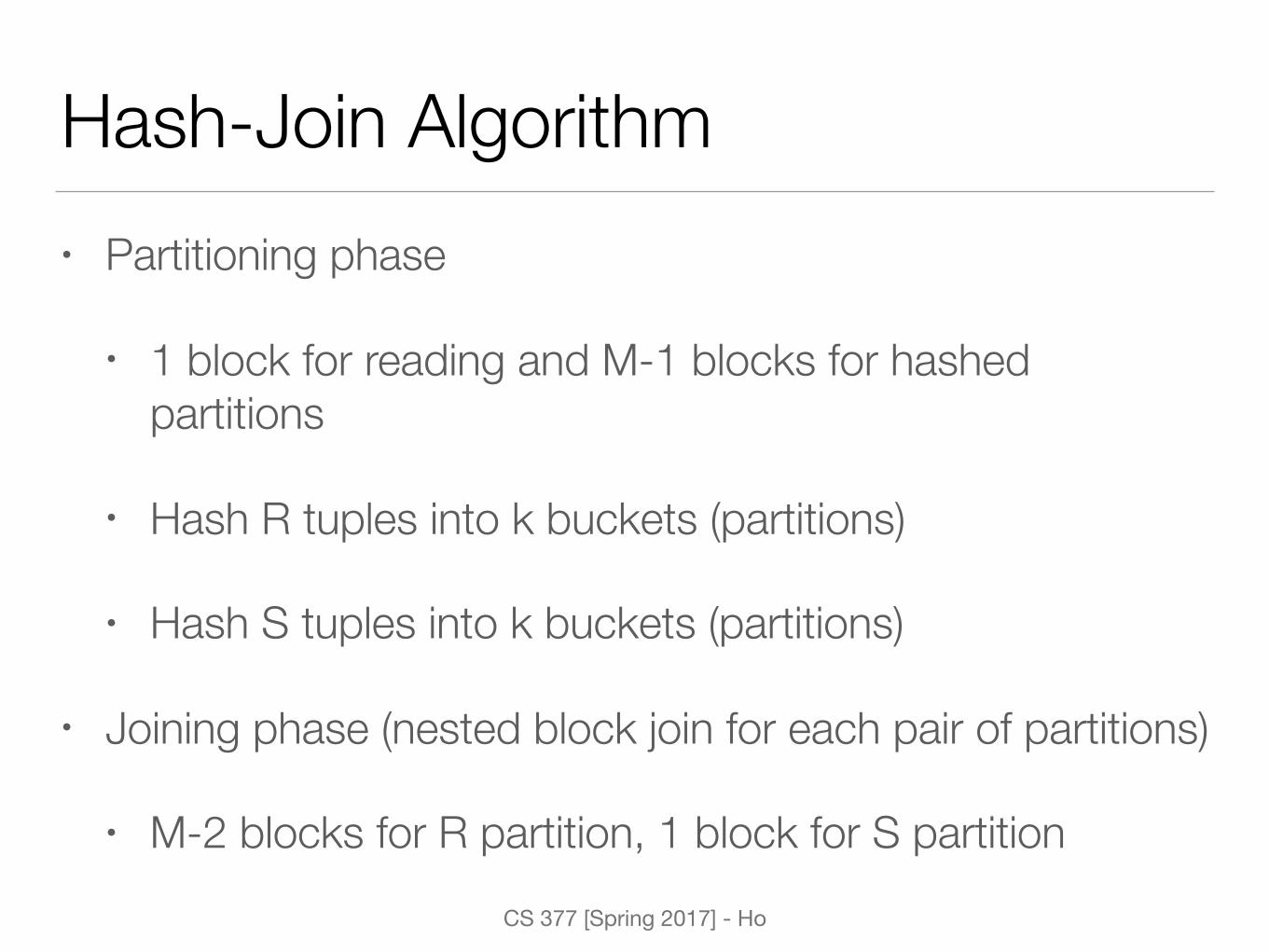
Hash-Join Algorithm• Partitioning phase
• 1 block for reading and M-1 blocks for hashed partitions
• Hash R tuples into k buckets (partitions)
• Hash S tuples into k buckets (partitions)
• Joining phase (nested block join for each pair of partitions)
• M-2 blocks for R partition, 1 block for S partition
CS 377 [Spring 2017] - Ho
Hash-Join Algorithm
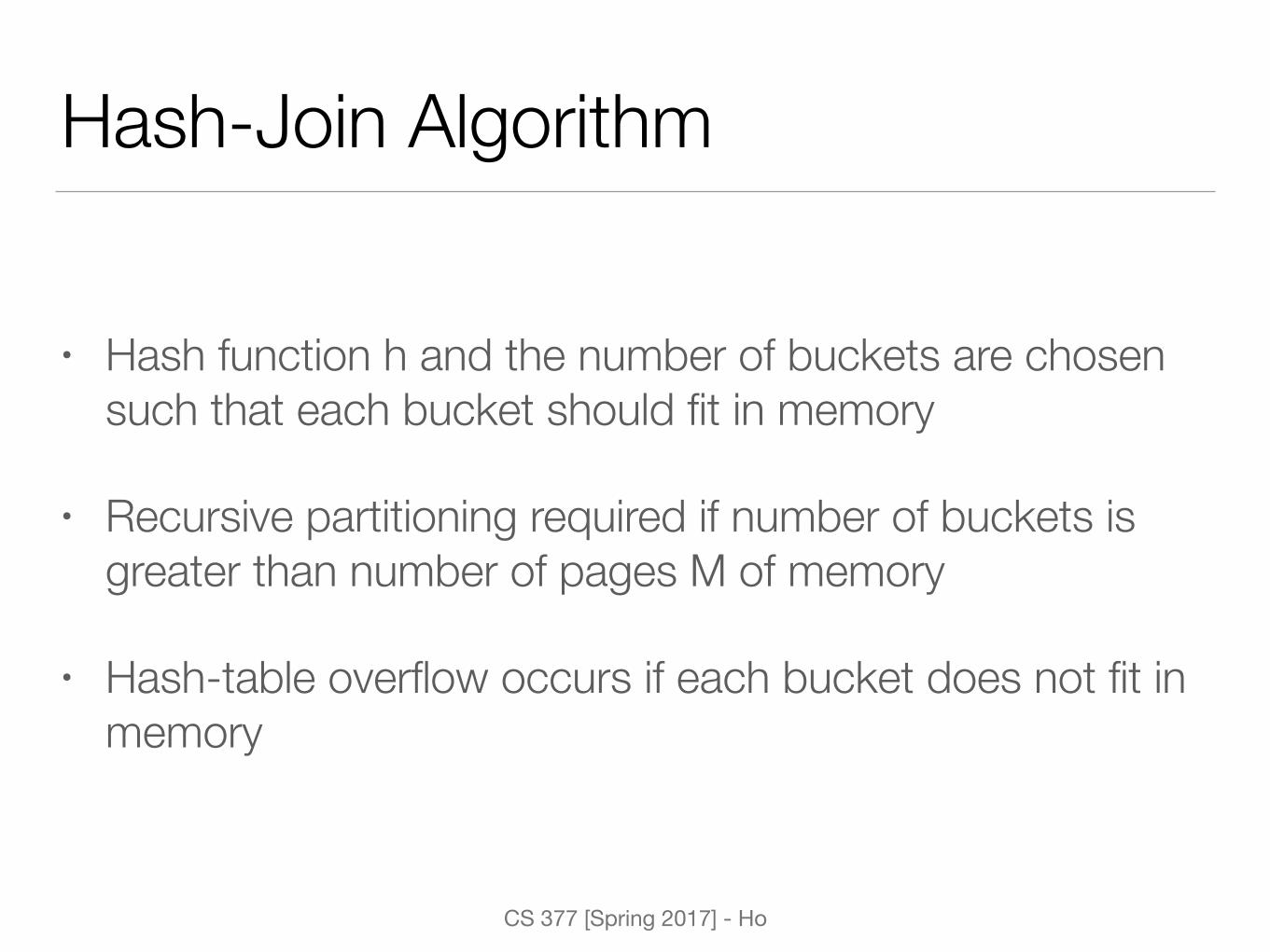
• Hash function h and the number of buckets are chosen such that each bucket should fit in memory
• Recursive partitioning required if number of buckets is greater than number of pages M of memory
• Hash-table overflow occurs if each bucket does not fit in memory

CS 377 [Spring 2017] - Ho
Hash-Join Cost• If recursive partitioning is not required:
• Partitioning phase: 2bR + 2bS
• Joining phase: bR + bS
• Total: 3bR + 3bS
• If recursive partitioning is required:
• Number of passes required to partition:
• Total cost:2(bR + bS)dlogM�1(bS)� 1e+ bR + bS
dlogM�1(bS)� 1e

CS 377 [Spring 2017] - Ho
Example: Hash-Join
• Assume memory size is 20 blocks
• What is cost of joining customer and depositor?
• Since depositor has less total blocks, we will use it to partition into 5 buckets, each of size 20 blocks
• Customer is also partitioned into 5 buckets, each of size 80 blocks
• Total cost: 3(100 + 400) = 1500 block transfers

CS 377 [Spring 2017] - Ho
Hash Join vs Sorted Join• Sorted join advantages
• Good if input is already sorted, or need output to be sorted
• Not sensitive to data skew or bad hash functions
• Hash join advantages
• Can be cheaper due to hybrid hashing
• Dependent on size of smaller relation — good for different relation sizes
• Good if input already hashed or need output hashed

CS 377 [Spring 2017] - Ho
Type Details Cost
Nested loop
Nested block
Indexed nested loop
Sort merge join
Hash join no recursive partitioning
Hash join recursive partitioning
JOIN Algorithms Cost
nRbS + bR
bRbS + bR
if both fit in memory: bR + bS
bR + nRc
sort cost + bR + bS
3bR + 3bS
2(bR + bS)dlogM�1(bS)� 1e+ bR + bS
CS 377 [Spring 2017] - Ho
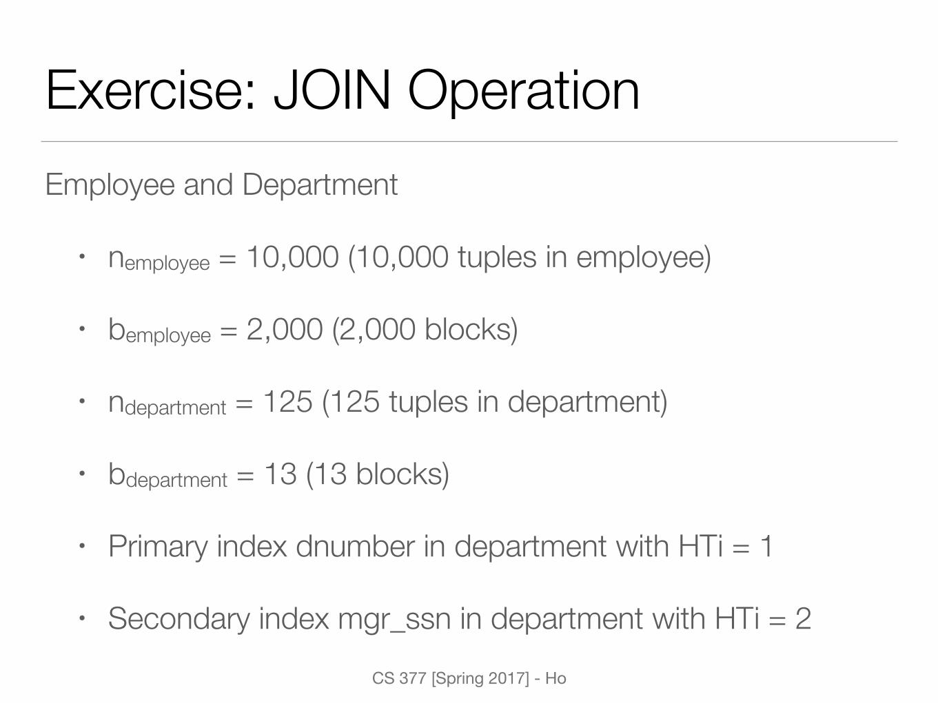
Exercise: JOIN OperationEmployee and Department
• nemployee = 10,000 (10,000 tuples in employee)
• bemployee = 2,000 (2,000 blocks)
• ndepartment = 125 (125 tuples in department)
• bdepartment = 13 (13 blocks)
• Primary index dnumber in department with HTi = 1
• Secondary index mgr_ssn in department with HTi = 2
CS 377 [Spring 2017] - Ho
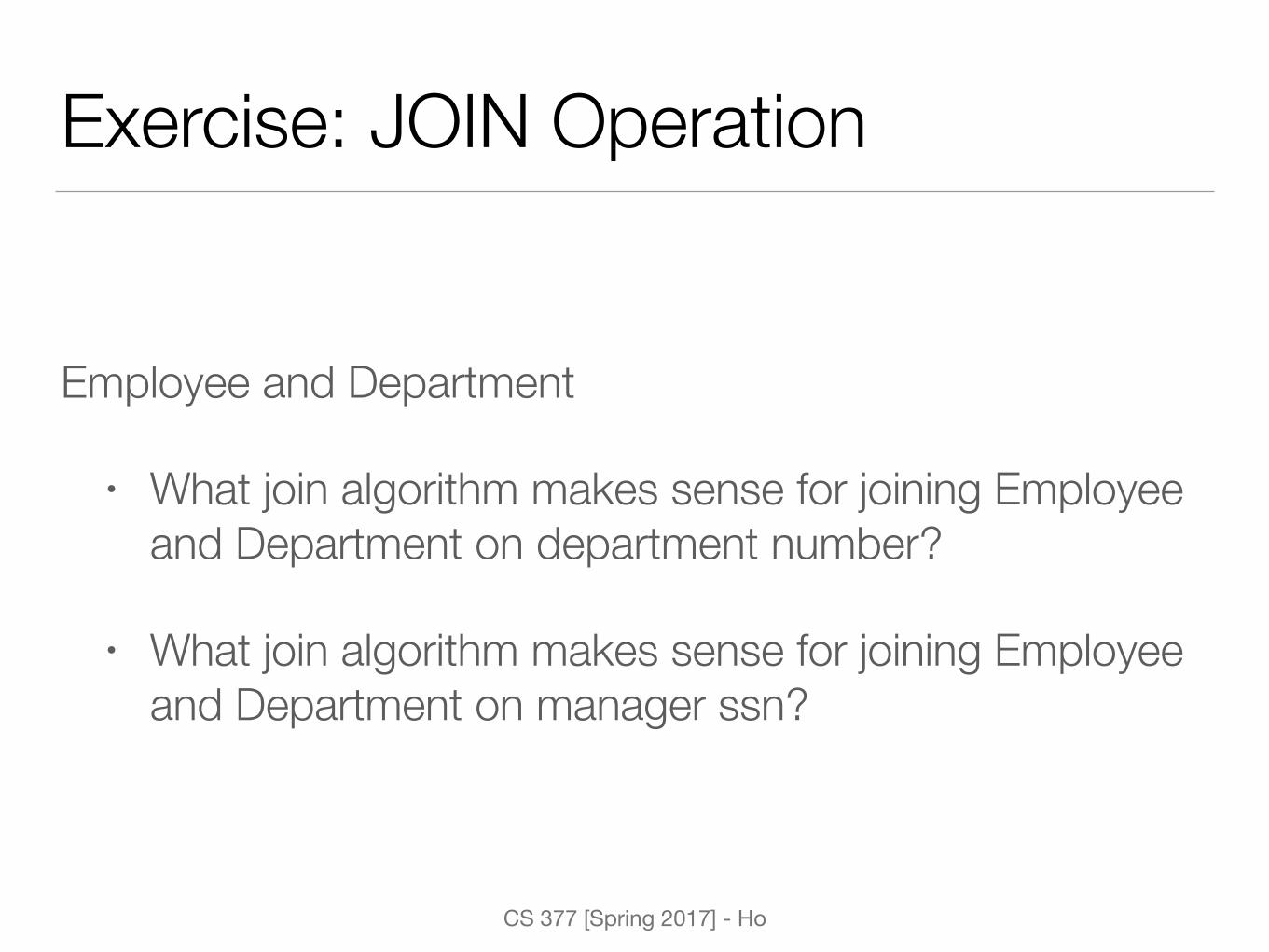
Exercise: JOIN Operation
Employee and Department
• What join algorithm makes sense for joining Employee and Department on department number?
• What join algorithm makes sense for joining Employee and Department on manager ssn?
CS 377 [Spring 2017] - Ho
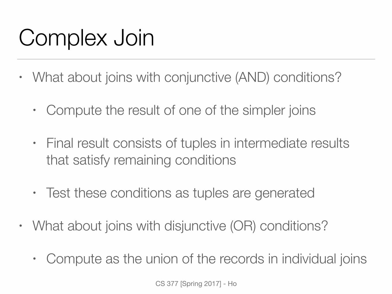
Complex Join• What about joins with conjunctive (AND) conditions?
• Compute the result of one of the simpler joins
• Final result consists of tuples in intermediate results that satisfy remaining conditions
• Test these conditions as tuples are generated
• What about joins with disjunctive (OR) conditions?
• Compute as the union of the records in individual joins
CS 377 [Spring 2017] - Ho
Example: Complex Join
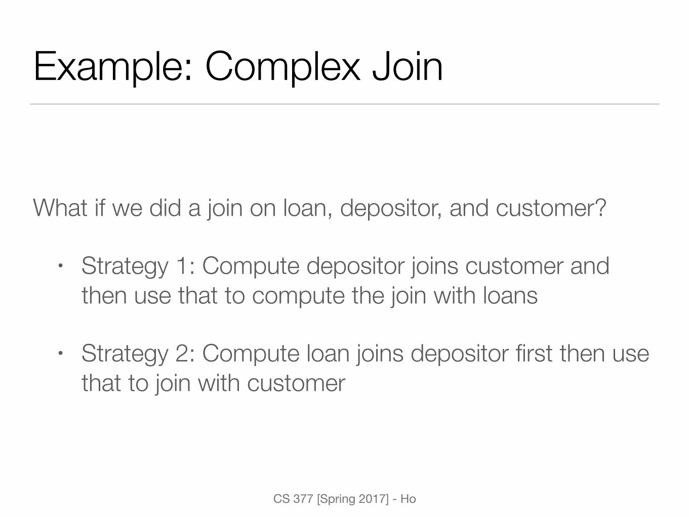
What if we did a join on loan, depositor, and customer?
• Strategy 1: Compute depositor joins customer and then use that to compute the join with loans
• Strategy 2: Compute loan joins depositor first then use that to join with customer

CS 377 [Spring 2017] - Ho
Example: Complex Join
What if we did a join on loan, depositor, and customer?
• Strategy 3: Perform pair of joins at once, build an index on loan for lID and on customer for cname
• For each tuple t in depositor, lookup corresponding tuples in customer and corresponding tuples in loan
• Each tuple of depositor is examined exactly once

CS 377 [Spring 2017] - Ho
PROJECT Algorithms
• Extract all tuples from R with only attributes in attribute list of projection operator & remove tuples
• By default, SQL does not remove duplicates (unless DISTINCT keyword is included)
• Duplicate elimination
• Sorting
• Hashing (duplicates in same bucket)
CS 377 [Spring 2017] - Ho
Aggregation Algorithms
Similar to duplicate elimination
• Sort or hash to group same tuples together
• Apply aggregate functions to each group

CS 377 [Spring 2017] - Ho
Set Operation Algorithms
• CARTESIAN PRODUCT
• Nested loop - expensive and should avoid if possible
• UNION, INTERSECTION, SET DIFFERENCE
• Sort-merge
• Hashing

CS 377 [Spring 2017] - Ho
Recap: Query Processing
SQL Query RA Plan Optimized RA Plan Execution
Declarative user query
Translate to RA expression
Find logically equivalent but
more efficient RA expression
Select physical algorithm with
lowest IO cost to execute the plan
CS 377 [Spring 2017] - Ho
DBMS’s Query Execution Plan
• Most commercial RDBMS can produce the query optimizer’s execution plan to try to understand the decision made by the optimizer
• Common syntax is EXPLAIN <SQL query> (used by MySQL)
• Good DBAs (database administrators) understand query optimizers VERY WELL!
CS 377 [Spring 2017] - Ho
Why Should I Care?• If query runs slower than expected, check the plan — DBMS
may not be executing a plan you had in mind
• Selections involving null values
• Selections involving arithmetic or string operations
• Complex subqueries
• Selections involving OR conditions
• Determine if you should build another index, or if index needs to be re-clustered or if statistics are too old
CS 377 [Spring 2017] - Ho
Query Tuning Guidelines• Minimize the use of DISTINCT — don’t need if duplicates are
acceptable or if answer already has a key
• Minimize use of GROUP BY and HAVING
• Consider DBMS use of index when using math
• E.age = 2 * D.age might only match index on E.age
• Consider using temporary tables to avoid “double-dipping” into a large table
• Avoid negative searches (can’t utilize indexes)
CS 377 [Spring 2017] - Ho
Query Optimization: Recap
• Query processing
• Cost-based optimization
• SELECT, JOIN algorithms
• Other operation algorithms (PROJECT, SET, Aggregate)


![SQL Introduction - Joyce Hojoyceho.github.io/cs377_s17/slide/7-sql-intro.pdf · CS 377 [Spring 2017] - Ho SQL DBMS • MySQL is the most popular, freely available database management](https://static.fdocuments.net/doc/165x107/5aa897577f8b9a7c188bcb6d/sql-introduction-joyce-377-spring-2017-ho-sql-dbms-mysql-is-the-most-popular.jpg)