Quasi-Linear Size Zero Knowledge fromLinear-Algebraic PCPs

Eli Ben-Sasson2, Alessandro Chiesa3, Ariel Gabizon2 and Madars Virza1

1 MIT2 Technion

3 UC Berkeley

Abstract. The seminal result that every language having an interactive proofalso has a zero-knowledge interactive proof assumes the existence of one-wayfunctions. Ostrovsky and Wigderson (ISTCS 1993) proved that this assumptionis necessary: if one-way functions do not exist, then only languages in BPP havezero-knowledge interactive proofs.Ben-Or et al. (STOC 1988) proved that, nevertheless, every language having amulti-prover interactive proof also has a zero-knowledge multi-prover interactiveproof, unconditionally. Their work led to, among many other things, a line ofwork studying zero knowledge without intractability assumptions. In this line ofwork, Kilian, Petrank, and Tardos (STOC 1997) defined and constructed zero-knowledge probabilistically checkable proofs (PCPs).While PCPs with quasilinear-size proof length, but without zero knowledge, areknown, no such result is known for zero knowledge PCPs. In this work, we showhow to construct “2-round” PCPs that are zero knowledge and of length O(K)where K is the number of queries made by a malicious polynomial time verifier.Previous solutions required PCPs of length at least K6 to maintain zero knowl-edge. In this model, which we call duplex PCP (DPCP), the verifier first receivesan oracle string from the prover, then replies with a message, and then receivesanother oracle string from the prover; a malicious verifier can make up to Kqueries in total to both oracles.Deviating from previous works, our constructions do not invoke the PCP Theo-rem as a blackbox but instead rely on certain algebraic properties of a specificfamily of PCPs. We show that if the PCP has a certain linear algebraic struc-ture — which many central constructions can be shown to possess, including[BFLS91,ALMSS98,BS08] — we can add the zero knowledge property at vir-tually no cost (up to additive lower order terms) while introducing only minormodifications in the algorithms of the prover and verifier. We believe that ourlinear-algebraic characterization of PCPs may be of independent interest, as itgives a simplified way to view previous well-studied PCP constructions.

1 Introduction

We continue the study of proof systems that provide soundness and zero knowledge,simultaneously and unconditionally (i.e., no intractability assumptions are needed toachieve the two), as we now explain.

Interactive proofs. An interactive proof [6, 20] for a language L is a pair of inter-active algorithms (P, V ), where P is known as the prover and V as the verifier, thatsatisfies the following: (i) (completeness) for every instance x in L , P (x) can makeV (x) accept with probability 1; (ii) (soundness) for every instance x not in L , everyprover P can make V (x) accept with at most a small probability ε. Shamir [35] showedthe expressive power of interactive proofs by proving that IP = PSPACE, i.e., alland only languages in PSPACE have interactive proofs.

Zero knowledge. An interactive proof is zero knowledge [20] if the verifier, evenif malicious, cannot learn any information about an instance x in L , by interactingwith the prover, besides the fact x is in L : for any efficient verifier V there exists anefficient simulator S such that S(x) is “indistinguishable” from the view of V whileinteracting with P (x). Depending on the choice of definition for indistinguishability,one gets different flavors of zero knowledge.

If indistinguishability is required to hold for efficient deciders only, then one getscomputational zero knowledge; CZK denotes the corresponding complexity class.A seminal result in cryptography says that if one-way functions exist then CZK =IP, i.e., every language having an interactive proof also has a computational zero-knowledge interactive proof [20, 23, 8]. If indistinguishability is required to hold forall deciders, then one gets statistical zero knowledge; if instead the simulator’s outputand the verifier’s view are the same distribution (and not merely close to each other),then one gets perfect zero knowledge. These stronger notions determine the correspond-ing complexity classes SZK and PZK, both of which are contained in AM∩coAM;of course, PZK ⊆ SZK ⊆ CZK.

Unfortunately, zero knowledge cannot be achieved unconditionally for non-triviallanguages: Ostrovsky and Wigderson [33] proved that if one-way functions do not existthen CZK equals an average-case variant of BPP.

Other types of proof systems. Due to the limitations of interactive proofs with respectto zero knowledge that holds unconditionally, researchers have explored other types ofproof systems, as an alternative to interactive proofs.

– MIP. Ben-Or et al. [9] first studied statistical zero knowledge, and proved that it canbe achieved in a new model, multi-prover interactive proof (MIPs), where the verifierinteracts with multiple provers that are not allowed to communicate while interactingwith the verifier (though they may share a random string before such an interactionbegins). More precisely, Ben-Or et al. prove that every language having a multi-prover interactive proof also has a perfect zero-knowledge multi-prover interactiveproof (again, without relying on intractability assumptions). The result of [9] wassubsequently improved in a number of papers [29, 5, 19].

– PCP. Kilian et al. [28] study statistical zero knowledge in the model of probabilisti-cally checkable proofs (PCPs) [4, 3, 2], where the verifier has oracle access to a string.Essentially, the oracle string can be thought of as a stateless prover: the answer to aquery depends only on the query itself, but not any other queries that were previouslymade. Building on results implicit in [19], Kilian et al. showed two main theorems.First, every language in NEXP has a PCP that is statistical zero knowledge againstverifiers that make at most any polynomial number of queries to the PCP. Second,

2

every language in NP has, for every constant c > 0, a PCP that is statistically zeroknowledge against verifiers that make at most k(n) := nc queries to the PCP.Subsequent works [24, 25, 31, 26] provided simplifications (giving alternative con-structions or simplifying that of [28]) and limitations (showing that for languages inNP one cannot efficiently sample the oracle if one seeks statistical zero knowledgeagainst verifiers that make at most a polynomial number of queries).

– IPCP. Goyal et al. [21] study statistical zero knowledge in the model of inter-active PCPs (IPCPs) [27], where the verifier interacts with two provers of whichone is restricted to be an oracle. Goyal et al. prove that every language in NP hasa constant-round interactive PCP that is statistical zero knowledge against verifiersthat make at most any polynomial number of queries to the PCP, and where bothprovers’ strategies can be implemented efficiently as a function of the instance andthe witness.

A limitation of prior work. PCPs with quasilinear-size proof length, but without zeroknowledge, are known: for every language L in NTIME(T (n)), there is a PCP withproof length O(T (n)) and query complexity O(1) [17, 15, 14, 32]. On the other hand,no such result for statistical zero knowledge PCPs is known: even when applied to PCPsof length O(T (n)), [28]’s result and followup improvements yields a proof length thatis polynomial in T (n) ·k(n), where k(n), known as the knowledge bound, is a bound onthe number of queries by any verifier (see Section 4.1 for further discussion). We thusask the following question: are there statistical zero knowledge PCPs with proof lengthquasilinear in T (n) + k(n)?

1.1 Our contributions

We do not answer the above question in the PCP model, but we give a positive answerin a closely related model that can be thought of as a “2-round PCP”, which we callduplex PCP (DPCP). At a high level, a DPCP works as follows: the prover first sendsan oracle string π0 to the verifier, just as in a PCP; then, the verifier sends a messageρ to the prover; finally, the prover answers with a second oracle string π1; the verifiermay query both oracles, and then accept or reject. In other words, a DPCP is merely a2-round interactive proof in which the prover sends oracle strings rather than messages.We prove the following theorem:

Theorem 1 (see Theorem 4 for formal statement). For every language L in NTIME(T )∩NP and polynomially-bounded knowledge bound k there exists a DPCP system satis-fying the following:– the proof length (in fact, also the prover running time) is quasilinear in n+ T (n) +k(n);

– the query complexity is polynomial in log(T (n) + k(n));– the verifier running time is polynomial in n+ log(T (n) + k(n));– perfect zero knowledge holds against any verifier that makes at most k(n) adaptive

queries (in total to both oracles);– the soundness error is 1/2 (and can be reduced by repetition to 2−λ while preserving

perfect zero knowledge, provided that the number of queries does not exceed k(n)).

3

Moreover, similarly to the PCPs of [28], the DPCP system that we construct is infact not only sound but is also a proof of knowledge [7]; however, in contrast to [28],the DPCP verifier is non-adaptive, in the sense that the query locations depend only onthe verifier’s random tape.

Perhaps the main difference between our construction and prior work is the tech-niques that we use. While previous works use the PCP Theorem as a black box, com-piling a PCP into a zero knowledge PCP by using locking schemes [28], we use certainalgebraic properties of a specific family of PCPs to guarantee zero knowledge. In com-parison to the generic approach, we are more specific, but the addition of zero knowl-edge essentially comes “for free” when compared to the corresponding constructionswithout zero knowledge. (In contrast, [28] achieves a proof length of Ω(k(n)6 · l(n)c),for some large enough c, when starting from a PCP with proof length l(n).)DPCP vs IPCP. Duplex PCPs are an alternative to interactive PCPs that combine PCPsand interaction. In a DPCP, the verifier gets an oracle string from the prover, replies witha message, and then gets another oracle string from the prover; in an IPCP, the verifiergets an oracle string from the prover, and then engages in an interactive proof with him.

Both [21] and our work are similar in that both address aspects that we do notnot know how to address in the PCP model, and resort to studying alternative models,i.e., IPCP and DPCP respectively. The two works however give different flavors ofresults: [21] obtain IPCPs that are zero knowledge against verifiers that ask at mostany polynomial number of queries k(n) but their oracle is of polynomial size in k(n)(actually, of exponential size but with a polynomial-size circuit describing it); on theother hand, our work obtains DPCPs that are zero knowledge against verifiers that askat most a fixed polynomial number of queries k(n) and our oracles are of quasilinearsize in k(n).

Finally, we note that our construction can be also cast as an IPCP, because theknowledge bound k(n) holds only for the first oracle, i.e., perfect zero knowledge ispreserved even if the verifier reads the second oracle in full. This provides a result on a2-round IPCP incomparable to [21]’s 4-round IPCP.On the minimal computational gap between prover and verifier needed for zeroknowledge. IP and MIP systems assume a computational gap between prover andverifier. The prover is allowed (and often assumed) to be computationally unboundedand the verifier is polynomially bounded. An intriguing corollary of our theorem isthat the computational gap between prover and verifier can be drastically reduced, toa mere polylogarithmic one. Namely, suppose that we wish to create zero-knowledgesystems in which the verifier runs in time tv(n); in the model above, as long as tp(n) >tv(n) · (log tv(n))c for an absolute constant c, then perfect zero knowledge with a smallsoundness error can be obtained under no intractability assumptions. (See Corollary 1for a formal statement.)

2 Preliminaries

Functions and distributions. We use f : D → R to denote a function with domainD and range R; given a subset D of D, we use f |D to denote the restriction of f to D.Given a distribution D, we write x← D to denote that x is sampled according to D.

4

Distances. A distance measure is a function ∆ : Σn × Σn → [0, 1] such that for allx, y, z ∈ Σn: (i) ∆(x, x) = 0, (ii) ∆(x, y) = ∆(y, x), and (iii) ∆(x, y) ≤ ∆(x, z) +∆(z, y). For example, the relative Hamming distance over alphabet Σ is a distancemeasure: ∆Ham

Σ (x, y) := |i |xi 6= yi|/n. We extend ∆ to distances of strings to sets:given x ∈ Σn and S ⊆ Σn, we define∆(x, S) := miny∈S ∆(x, y) (or 1 if S is empty).We say that a string x is ε-close to another string y if ∆(x, y) ≤ ε, and ε-far from y if∆(x, y) > ε; similar terminology applies for a string x and a set S.

Fields and polynomials. We denote by F a finite field, by Fq the field of size q, and byF the set of all finite fields. We denote by F[X1, . . . , Xm] the ring of polynomials inmvariables over F; given a polynomial P in F[X1, . . . , Xm], degXi(P ) is the degree ofP in the variable Xi; the total degree of P is the sum of all of these individual degrees.

Linear spaces. Given n ∈ N, a subset S of Fn is an F-linear space if αx + βy ∈ Sfor all α, β ∈ F and x, y ∈ S.

Languages and relations. We denote by R a relation consisting of pairs (x,w),where x is the instance and w is the witness. We denote by Lan(R) the languagecorresponding to R, and by R|x the set of witnesses in R for x.

Complexity classes. We write complexity classes in bold capital letters: NP, PSPACE,NEXP, and so on. We take a “relation-centric” point of view: we view NTIME as aclass of relations rather than as the class of the corresponding languages; we thus maywrite things like “let R be in NP”. If R is in NTIME(T ), we fix an arbitrary ma-chine MR that decides R in time T (n), i.e., MR(x,w) always halts after T (|x|) stepsand MR(x,w) = 1 if and only if (x,w) ∈ R; we then say that MR decides R (orLan(R)). Throughout, we assume that T (n) ≥ n.

Codes. An error correcting code C is a set of functions w : H → Σ, where H,Σ arefinite sets. The message length of C is n := log|Σ| |C|, its block length is ` := |H|,its rate is ρ := n/`, its (minimum) distance is d := min∆(w, z) |w, z ∈ C , w 6= zwhen ∆ is the (absolute) Hamming distance, and its (minimum) relative distance isδ := d/`. Given a code family C , we denote by Rel(C ) the relation that naturallycorresponds to C , i.e., (C,w) | C ∈ C , w ∈ C. A code C is linear if Σ is a finitefield and C is a Σ-linear space in Σ`; we denote by dim(C) the dimension of C whenviewed as a linear space. A code C is t-wise independent if, for every subset I of [`]with cardinality t, the distribution of w|I (viewed as a string) for a random w ∈ Cequals the uniform distribution on Σt.

Random shifts. We later use the following folklore claim about distance preservationfor random shifts in linear spaces; for completeness, we include its short proof.

Claim. Let n be in N, F a finite field, S an F-linear space in Fn, and x, y ∈ Fn. If x isε-far from S, then αx+ y is ε/2-far from S, with probability 1− |F|−1 over a randomα ∈ F. (Distances are relative Hamming distances.)

Proof. Suppose, by way of contradiction, that there exist α1, α2 ∈ F and y1, y2 ∈ Swith α1 6= α2 such that, for every i ∈ 1, 2, αix + y is ε/2 close to yi. Then, by thetriangle inequality, z := y1 − y2 is ε-close to (α1x + y) − (α2x + y) = (α1 − α2)x.We conclude that x is ε-close to 1

α1−α2z ∈ S, a contradiction.

5

2.1 Probabilistically checkable proofs

A PCP system [4, 3, 2] for a relation R is a tuple PCP = (P, V ) that works as follows.

– The prover P is a probabilistic algorithm that, given as input an instance-witness pair(x,w) with n := |x|, outputs a proof π : D(n)→ Σ(n), where both D(n) and Σ(n)are finite sets.

– The verifier V is a probabilistic oracle algorithm that, given as input an instance xwith n := |x| and with oracle access to a proof π : D(n)→ Σ(n), queries π at a fewlocations and then outputs a bit.

The system PCP has (perfect) completeness and soundness error e(n) if the followingtwo conditions hold. (Below, we explicitly denote the prover’s and verifier’s randomnessas rP and rV .)

Completeness: For every instance-witness pair (x,w) in the relation R,

PrrP ,rV

[V P (x,w;rP )(x; rV ) = 1

]= 1 .

Soundness: For every instance x not in the language Lan(R) and proof π : D(n) →Σ(n),

PrrV

[V π(x; rV ) = 1] ≤ e(n) .

A relation R belongs to the complexity class PCP[a, l, q, e, tp, tv] if there is a PCPsystem for R in which:– the answer alphabet (i.e., Σ(n)) is a(n),– the proof length over that alphabet (i.e., |D(n)|) is at most l(n),– the verifier queries the proof in at most q(n) locations,– the soundness error is e(n),– the prover runs in time tp(n), and– the verifier runs in time tv(n).Finally, we add the symbol na in the square brackets (i.e., we write PCP[. . . ,na]) ifthe queries to the proof are non-adaptive (i.e., the queried locations only depend on theverifier’s inputs).

2.2 Probabilistically checkable proofs of proximity

A PCPP system [12, 18] for a relation R is a tuple PCPP = (P, V ) that works asfollows.

– The prover P is a probabilistic algorithm that, given as input an instance-witness pair(x,w) with n := |x|, outputs a proof π : D(n)→ Σ(n), where both D(n) and Σ(n)are finite sets.

– The verifier V is a probabilistic oracle algorithm that, given as input an instance xwith n := |x| and with oracle access to a witness w and proof π : D(n) → Σ(n),queries w and π at a few locations and then outputs a bit.

6

The system PCPP has (perfect) completeness, soundness error e, distance measure ∆,and proximity parameter d if the following two conditions hold. (Below, we explicitlydenote the prover’s and verifier’s randomness as rP and rV .)

Completeness: For every instance-witness pair (x,w) in the relation R,

PrrP ,rV

[V (w,P (x,w;rP ))(x; rV ) = 1

]= 1 .

Soundness: For every instance-witness pair (x,w), perhaps not in the language, suchthat ∆(w,R|x) ≥ d(n) and proof π : D(n)→ Σ(n),

PrrV

[V (w,π)(x; rV ) = 1

]≤ e(n) .

A relation R belongs to the complexity class PCPP[a, l, q, ∆, d, e, tp, tv] if there is aPCPP system for R in which:– the answer alphabet (i.e., Σ(n)) is a(n),– the proof length over that alphabet (i.e., |D(n)|) is at most l(n),– the verifier queries the two oracles (codeword and proof) in at most q(n) locations

(in total),– the distance measure is ∆,– the proximity parameter is d(n),– the soundness error is e(n),– the prover runs in time tp(n), and– the verifier runs in time tv(n).Finally, we add the symbol na in the square brackets (i.e., we write PCPP[. . . ,na])if the queries to the oracles are non-adaptive (i.e., the queried locations only depend onthe verifier’s inputs).

2.3 Zero knowledge PCPs

The notion of zero knowledge for PCPs was first considered in [19, 28]. A PCP systemPCP = (P, V ) for a relation R has perfect zero knowledge with knowledge bound k ifthere exists an expected-polynomial-time probabilistic algorithm S such that, for everyk-query polynomial-time probabilistic oracle algorithm V , the following two distribu-tion families are identical:

S(V , x)(x,w)∈R and PCPView(V , P, x,w)(x,w)∈R ,

where PCPView(V , π, x,w) is the view of V in its execution when given input xand oracle access to π := P (x,w). The definition of statistical and computationalzero knowledge (with knowledge bound k) are similar: rather than identical, the twodistribution families are required to be statistically and computationally close (as |x|grows), respectively.

A relation R belongs to the complexity class PCPpzk[a, l, q, e, tp, tv, k] if thereexists a PCP system for R that (i) puts R in PCP[a, l, q, e, tp, tv], and (ii) has perfectzero knowledge with knowledge bound k; as for PCP, we add the symbol na in the

7

square brackets of PCPpzk if the queries to the proof are non-adaptive. The complexityclasses PCPszk and PCPczk are similarly defined for statistical and computationalzero knowledge.

The KPT result. Kilian, Petrank, and Tardos proved the following theorem:

Theorem 2 ([28]). For every polynomial time function T : N→ N, polynomial securityfunction λ : N→ N, and polynomial knowledge bound function k : N→ N,

NTIME(T ) ⊆ PCPszk

a = F2poly(λ)

l = poly(T, k)q = poly(λ)e = 2−λ

tp = poly(λ, T )tv = poly(λ, T, k)k

.

Remark 1. We make two remarks: (i) the symbol na does not appear above because[28]’s construction relies on adaptively querying the proof; (ii) inspection of [28]’s con-struction reveals that l(n) ≥ poly(T (n)) · k(n)6.

2.4 Reed–Muller and Reed–Solomon codes

We define Reed–Muller and Reed–Solomon codes, as well as their “vanishing” variants[15]; all of these are linear codes. We then state a theorem about PCPPs for certainfamilies of RS codes.

RM codes. Let F be a finite field,H,V subsets of F,m a positive integer, and % a con-stant in (0, 1]; % is called the fractional degree. The Reed–Muller code with parametersF, H,m, % is RM[F, H,m, %] := w : Hm → F | maxi∈[m] degXi(w) < %|H|; itsmessage length is n = (%|H|)m, block length is ` = |H|m, rate is ρ = %m, and relativedistance is δ = 1− %. The vanishing Reed–Muller code with parameters F, H,m, %, Vis VRM[F, H,m, %, V ] := w ∈ RM[F, H,m, %] | w(V m) = 0; it is a subcode ofRM[F, H,m, %].

RS codes. Let F be a finite field, H,V subsets of F, and % a constant in (0, 1]. TheReed–Solomon code with parameters F, H, % is RS[F, H, %] := RM[F, H, 1, %]. Thevanishing Reed–Solomon code with parameters F, H, %, V is VRS[F, H, %, V ] := w ∈RS[F, H, %] | w(V ) = 0.Two RS code families and their PCPPs. Given % ∈ (0, 1], we denote by: (i)RS∗% theset of Reed–Solomon codes RS[F, H, %] for which F has characteristic 2 andH is an F2-affine space; and (ii) VRS∗% the set of vanishing Reed–Solomon codes VRS[F, H, %, V ]for which F has characteristic 2 and H is an F2-affine space. The following theoremis from [15, 10] (the prover running time is shown in [10] and the other parameters in[15]).

8

Theorem 3. For every security function λ : N→ N, % ∈ (0, 1), and s > 0,

Rel(RS∗%) , Rel(VRS∗%) ∈ PCPP

a = F2s+log `

l = O(`)q = λ · polylog(`)∆ = ∆Ham

a

d = %/2e = 2−λ

tp = poly(s) · O(`)tv = λ · poly(s+ log `)na

.

We will also require the following folklore claim, whose correctness can be provedby induction on m:

Claim. Let F be a finite field, H,V subsets of F with H ∩ V = ∅, m a positive integer,and t a positive integer not exceeding |H|−|V |. Then VRM[F, H,m, |V |+t|H| , V ] is t-wiseindependent.

3 Duplex PCPs

We define duplex PCPs, and then define notions of zero knowledge for this model.Our main theorem is the construction of a duplex PCP with certain parameters; seeSection 4. The difference between a PCP and a duplex PCP is that all provers (bothhonest and malicious) produce two proof oracles rather than one: the prover producesa proof π0; then the verifier sends a message ρ to the prover; then the prover producesanother proof π1; finally the verifier queries both π0 and π1 and either accepts or rejects.(Thus, a PCP is a special case of a duplex PCP, but not vice versa.) More precisely, aduplex PCP system for a relation R is a tuple DPCP = (P, V ) that works as follows.

– The prover P is a pair (P0, P1) of probabilistic algorithms, with shared randomness,where: (a) given as input an instance-witness pair (x,w) with n := |x|, P0 outputsa proof π0 : D0(n) → Σ(n); (b) given as input (x,w) and the verifier’s message ρ(see below), P1 outputs a proof π1 : D1(n) → Σ(n). Here D0(n), D1(n), Σ(n) arefinite sets.

– The verifier V is a pair (V0, V1) of probabilistic algorithms, with shared random-ness, where: (a) given as input an instance x with n := |x|, V0 outputs a messageρ; (b) given as input x and with oracle access to proofs π0 : D0(n) → Σ(n) andπ1 : D1(n)→ Σ(n), V1 queries π0 and π1 at a few locations and then outputs a bit.

The system DPCP has (perfect) completeness and soundness error e(n) if the followingtwo conditions hold. (Below, we explicitly denote the prover’s and verifier’s randomnessas rP and rV .)

Completeness: For every instance-witness pair (x,w) in the relation R,

PrrP ,rV

V π0,π1

1 (x; rV ) = 1

∣∣∣∣∣∣π0 ← P0(x,w; rP )

ρ← V0(x; rV )π1 ← P1(x,w, ρ; rP )

= 1 .

9

Soundness: For every instance x not in the language Lan(R) and pair of algorithmsP = (P0, P1),

PrrV

V π0,π1

1 (x; rV ) = 1

∣∣∣∣∣∣π0 ← P0

ρ← V0(x; rV )

π1 ← P1(ρ)

≤ e(n) .

A relation R belongs to the complexity class DPCP[a, l, q, e, tp, tv] if there is a DPCPsystem for R in which:– the answer alphabet (i.e., Σ(n)) is a(n),– the proof length over that alphabet (i.e., (|D0(n)|+ |D1(n)|)) is at most l(n),– the verifier queries the two proofs in at most q(n) locations (in total),– the soundness error is e(n),– the prover runs in time tp(n), and– the verifier runs in time tv(n).Finally, we add the symbol na in the square brackets (i.e., we write DPCP[. . . ,na]) ifthe queries to the proof are non-adaptive (i.e., the queried locations only depend on theverifier’s inputs).Zero knowledge. A DPCP system DPCP = (P, V ) for a relation R has perfect zeroknowledge with knowledge bound k if there exists an expected-polynomial-time prob-abilistic algorithm S such that for every pair of polynomial-time probabilistic oraclealgorithms V := (V0, V1) the following two distribution families are identical:

S(V , x)(x,w)∈R and DPCPView(k, V , P, x,w)(x,w)∈R ,

where DPCPView(k, V , P, x,w) is the view of V1 in its execution when given inputx and when allowed to make a total of k(n) adaptive queries to π0, π1, where π0 :=P0(x,w) and π1 := P1(x,w, V

π00 (x)). (As above, P0, P1 share the same randomness

rP ; ditto for V0, V1.) The definition of statistical and computational zero knowledge(with knowledge bound k) are similar: rather than identical, the two distribution familiesare required to be statistically and computationally close (as |x| grows), respectively.

4 Main theorem

The main result of this paper is the following.

Theorem 4. For every polynomial time function T : N → N, polynomial knowledgebound function k : N→ N,

NTIME(T ) ⊆ DPCPpzk

a = F2O(log(T+k))

l = O(T + k)q = polylog(T + k)e = 1

2

tp = poly(n) · O(T + k)tv = poly(n+ log(T + k))kna

10

A corollary. The theorem above implies that, fixing T , the prover running time ismerely quasilinear in the knowledge bound k, while the verifier running time increasesonly polylogarithmically in k. This leads to an intriguing corollary: a poly-logarithmiccomputational overhead of the prover over the verifier is all that is needed to maintainperfect zero knowledge in the duplex PCP model. We state this formally next.

Corollary 1. For every polynomial time function T : N→ N and relation R ∈ NTIME(T ),there is a constant c such that, for every function tv : N → N with tv(n) ≥ n ·(log T (n))c, there is a DPCP system with:– completeness 1 and soundness 2−tv(n)/polylog(T (n));– perfect zero knowledge;– the verifier running time is tv(n) and prover running time is tp(n) := maxT (n) ·(log T (n))c, tv(n) · (log tv(n))c.

The verifier has no limitations other than a bound on its running time (its query com-plexity can be as large as tv(n)).

4.1 Proof sketch

Let R be a relation in NP, and let (x,w) be an instance-witness pair in R. The proverand verifier both know x, while the prover also knowsw. The prover wishes to convincethe verifier that he knows a witnessw for x, in such a way that the verifier does not learnanything about w (beyond what can be inferred from the prover’s claim).The KPT approach. We introduce our ideas by contrasting them with those of [28].Suppose that the prover wishes to convince the verifier by sending him a PCP proofπ = π(w) such that any k values in π do not reveal anything aboutw. Loosely speaking,[28] (building on [19]) provide a probabilistic transformation that maps the PCP proofπ to a new proof π′, in which each bit of π is “hidden” amongst many bits of π′. Themain tool employed in the transformation is a locking scheme, and its use imposescertain limitations: (i) the new proof π′ is poly(k) larger than the original one (k6 byinspection of [19, 28]); (ii) zero knowledge holds only statistically, but not perfectly,because a malicious verifier can be “lucky” and obtain information on the bit of π beinglocked with fewer queries to π′ than expected.Our approach (ideally). We take a different approach: apply a “local” PCP to a “ran-dom” witness, as we now explain. Suppose that π = π(w) is (t, k)-local, i.e., any kpositions of the PCP proof π jointly depend on at most t positions of the witness w.Note that, even if π is (t, k)-local, a single bit of π can still leak information aboutw. So suppose further that the relation R is t-randomizable: given (x,w) ∈ R, onecan efficiently sample a witness w′ from a t-wise independent subset of the set of wit-nesses for x. In such a case, the prover can produce a zero-knowledge PCP as follows:(1) sample a witnessw′ from the t-wise independent subset; then (2) send to the verifierthe PCP proof π = π(w′). Indeed, the locality of π ensures that seeing any k indices ofπ reveals nothing about w, because these k indices are a function of t random bits. Insum, if we had a (t, k)-local PCP for a t-randomizable relation R, then we could obtaina PCP for R that is zero knowledge against verifiers that ask at most k queries.Our approach (in reality). Unfortunately, we do not know how to obtain local PCPsfor randomizable relations. However, we are able to obtain “partially local” duplex PCPs

11

for certain randomizable relations, and also show that NTIME can be efficiently re-duced to these randomizable relations, as we now explain.

Our starting point are algebraic PCPs: certain PCPs that prove satisfiability of al-gebraic problems (APs) [34]. Numerous known PCP constructions can be viewed asalgebraic PCPs. Informally, in this work we make two basic observations: (i) algebraicPCPs exist for certain randomizable relations; and (ii) an algebraic PCP proof can besplit in two parts, one part is local, while the other part is not local but enjoys conve-nient linear algebraic properties that, nevertheless, enable us to hide information aboutthe witness, in the duplex PCP model. (Recall that, in the duplex PCP model, the proverproduces a proof π0; then the verifier sends a message ρ to the prover; then the proverproduces another proof π1; finally the verifier queries both π0 and π1 and either acceptsor rejects.)

In more detail, from a technical viewpoint, we proceed as follows. First, we intro-duce a family of constraint satisfaction problems (CSPs) called linear algebraic CSPs,and show that NTIME is efficiently reducible to randomizable linear algebraic CSPs.The reduction consists of two parts: we go through an intermediary that we call grouppreserving algebraic problems (GAPs), a special case of APs that we believe to be of in-dependent interest for the study of algebraic PCPs. Second, we construct a duplex PCPsystem for randomizable linear algebraic CSPs that is zero knowledge against verifiersthat ask at most a certain number of queries.

A technical piece: zero-knowledge duplex PCPP for low-degreeness. Later sectionsaddress all of the above steps (see Section 4.2 for a roadmap of these), and for now weonly sketch one of these steps. Above we mention that an algebraic PCP proof has twoparts: a local part, and a non-local part. This latter part of the proof arises from a centralcomponent of many PCP proofs: a PCP of proximity (PCPP) [13, 18] that facilitateslow-degree testing. Informally, given a function f : H → F and an integer d, a PCPPfor degree d is a proof π(f) that f is ε-close to an evaluation of a polynomial degree atmost degree d. We explain how to transform a PCPP for low-degreeness into a duplexPCPP for low-degreeness that is zero knowledge against verifiers that make at most tqueries.

The set C of functions f : H → F that are evaluations of a polynomial of degree atmost d is a subspace of F|H|. The basic idea is that, in order for the prover to convincethe verifier that a function f is close to C, it suffices for the prover to convince theverifier that a random offset of f is close to C: one can verify that, for any u : H → F,if f is ε-far from C, then αf + u is ε/2-far from C, with probability 1 − |F|−1 overa random α ∈ F. Hence, we can let the duplex PCP work as follows: (i) the proversamples a witness w′ from the t-wise independent subset, chooses a random u ∈ C,and sends π0 := (w′, u) to the verifier; (ii) the verifier sends to the prover a randomα ∈ F; (iii) the prover sends π1 = (v, π(v)) to the verifier, where v := αw′ + u andπ(v) is a PCPP for low-degreeness of v; (iv) the verifier runs the PCPP verifier on (v, π)to check that v is close to C, and then checks that vi = αw′i + ui for a few randomindices i in 1, . . . , |H|.

Let us discuss the various properties of the duplex PCPP.– COMPLETENESS: If w ∈ C, then αw′ + u ∈ C; therefore, the prover convinces the

verifier.

12

– ZERO-KNOWLEDGE: If the verifier asks at most t queries, then he learns nothingabout w because: π0 = (w′, u) contains w′ sampled from a t-wise independentsubset and u random in C; π1 = (v, π(v)) is running the PCPP on a vector v that israndom in C.

– SOUNDNESS: If v does equal α ·w+u, then the verifier rejects with high probabilitybecause v is far from C (and the PCPP verifier rejects π with high probability).If instead v does not equal α · w + u, then the fact that v is close to C does notprove anything about whether w is also close. So, in this case, we need to reasonabout the success probability of the verifier’s linearity tests: if these pass with enoughprobability, then with high probability v is close to αw+ u, which again suffices forour purpose. Overall, soundness holds.

Next, we discuss how the technical sections are organized, and how they come togetherto yield our main theorem.

4.2 Roadmap of the rest of the paper

The rest of the paper is dedicated to turn the above intuition into a more formal proof.To do so, we introduce various intermediate steps, as follows.– In Section 5, we introduce linear algebraic CSPs (a family of constraint satisfaction

problems), and then describe how to obtain a canonical PCP for any linear algebraicCSP.

– In Section 6, we introduce randomizable linear algebraic CSPs, a subfamily of linearalgebraic CSPs; then we show that, for every randomizable linear algebraic CSP, wecan convert the CSP’s canonical PCP into a corresponding zero-knowledge duplexPCP, incurring only little overheads.

– In Section 7, we show an efficient reduction from NTIME to randomizable linearalgebraic CSPs; along the way, we introduce a family of algebraic problems, havingspecial symmetry properties, that we believe to be of independent interest (e.g., forstudying other questions about PCPs).

Combining (i) the efficient reduction from NTIME to randomizable linear algebraicCSPs together with (ii) the zero-knowledge duplex PCP for such problems yields The-orem 4. In Section 8 we provide details about how these components are combined.

5 Linear algebraic CSPs and their canonical PCPs

We introduce linear algebraic CSPs, a family of constraint satisfaction problems; thenwe describe how to obtain a canonical PCP for any linear algebraic CSP.

5.1 Linear algebraic constraint satisfaction problems

A constraint satisfaction problem asks whether, for a given “local” function g, thereexists an input α such that g(α) is an “accepting” output. For example, in the case of 3-SAT with n variables and m clauses, the function g maps 0, 1n to 0, 1m, and g(α)indicates which clauses are satisfied by α ∈ 0, 1n; hence α yields an accepting outputif (and only if) g(α) = 1m. Below we introduce a family of constraint satisfaction

13

problems whose domain and range are linear-algebraic objects, namely, linear errorcorrecting codes.

We begin by providing the notion of locality that we use for g; we also provide twoother notions, one for the efficiency of computing a single coordinate of g’s output, andanother for measuring g’s “pseudorandomness”.

Definition 1. Let g : Σn → Σm be a function. We say that g is:– q-local if for every j ∈ [m] there exists Ij ⊆ [n] with |Ij | ≤ q such that g(α)[j] (thej-th coordinate of g(α)) depends only on α|Ij (the restriction of α to Ij);

– c-efficient if there is a time c algorithm that, given j and α|Ij , computes the set Ijand value g(α)[j];

– (γ, ε)-sampling if Pr[ Ij ∩ I 6= ∅ | j ← [m] ] ≤ γ for every I ⊆ [n] with |I|/n ≤ ε.

Next we introduce RLA, the relation of linear algebraic CSPs:

Definition 2 (RLA). Given functions f : N → F , `, q, c : N → N, and ρ, δ, γ, ε : N →(0, 1], the relation

RLA[f, `, ρ, δ, q, c, γ, ε]

consists of instance-witness pairs (x,w) satisfying the following.

– The instance x is a tuple (1n, C, C•, g) where:• C, C• are linear error correcting codes with block lengths `(n), `•(n) at most`(n), each with rate at most ρ(n) and relative distance at least δ(n) over the samefield f(n);

• g : f(n)`(n) → f(n)`•(n) is a q(n)-local, c(n)-efficient, (γ(n), ε(n))-samplingfunction;

• C• ∪ g(C) has relative distance at least δ(n) (though may not be a linear space).– The witness w is a tuple (α, α•) where α ∈ f(n)`(n) and α• ∈ f(n)`•(n).– The instance x and witness w jointly satisfy the following: α ∈ C, α• ∈ C•, andg(α) = α•.

We prove a simple claim about instances not in the language Lan(RLA), which weuse several times later on.

Claim. For every instance x = (1n, C, C•, g) not in the language Lan(RLA) and (can-didate) witness w = (α, α•) ∈ f(n)`(n) × f(n)`•(n) at least one of the followingholds:– at least one of α and α• is ε-far in relative Hamming distance from C or C•,

respectively; or– there exist α ∈ C and α• ∈ C• such that α and α• are ε-close to α and α•,

respectively, but g(α) 6= α•.

Proof. If neither of the two cases hold, then there exist α ∈ C and α• ∈ C• suchthat g(α) = α•. But then (α, α•) is a satisfying assignment for x, contradicting ourassumption that x is not in the language Lan(RLA).

Finally we need notation for referring to codes appearing in instances of RLA:

14

Definition 3. Given R ⊆ RLA, we denote by– CR, the set of codes C for which there is an instance x = (1n, C, C•, g) in the

relation R with C = C;– CR,• the set of codes C for which there is an instance x = (1n, C, C•, g) in the

relation R with C = C•.

5.2 A canonical PCP for linear algebraic CSPs

We show how to construct a “canonical” PCP system for instances in RLA (the relationof linear algebraic CSPs). At a high level, a canonical PCP proof for a RLA-instance xconsists of a witnessw = (α, α•) concatenated with two PCPP proofs π, π•, showingthat α, α• are close to C, C• respectively. The canonical PCP verifier first checksthe two PCPP proofs and then checks that g(α)[j] = α•[j] for a uniformly randomj ∈ [`•].

Definition 4. Given (i) a relation R ⊆ RLA, (ii) a PCPP system PCPP = (P, V)for Rel(CR,), and (iii) a PCPP system PCPP• = (P•, V•) for Rel(CR,•), the canon-ical PCP system for the triple (R,PCPP,PCPP•) is the PCP system PCP = (P, V )constructed as follows.

– Prover. Given (x,w) ∈ RLA, the PCP prover P outputs π := (w, π, π•) whereπ := P(C, α) and π• := P•(C•, α•). In other words, the PCP prover outputs aPCP proof that is the concatenation of the witnessw = (α, α•) and a pair of PCPPproofs, the first proving that α ∈ C and the second proving that α• ∈ C•.

– Verifier. Given x and oracle access to a PCP proof π = (w, π, π•), the PCP verifierV works as follows:• (proximity) check that V (α,π)

(C) and V (α•,π•)• (C•) both accept;

• (consistency) check that g(α)[j] = α•[j] for a uniformly random j ∈ [`•].

The next lemma says that the above construction is a PCP system when RLA’sparameters are sufficiently “good”.

Lemma 1 (RLA → PCP). Suppose that R is a relation that satisfies the followingconditions:

(i) R ⊆ RLA[f1, `1, ρ1, δ1, q1, c1, γ1, ε1] with ε1 < min δ12 , δ1 − γ1;(ii) Rel(CR,),Rel(CR,•) ∈ PCPP[a2, l2, q2, ∆

Hama2 , d2, e2, tp2, tv2,na?] with a2 =

f1 and d2 ≤ ε1.Then there is a canonical PCP system for a triple (R,PCPP,PCPP•) that yields

R ∈ PCP

a = f1 (= a2)l = 2l2(`1) + 2`1q = 2q2(`1) + q1 + 1e = max1− δ1 + γ1 + ε1, e2tp = 2tp2(`1)tv = 2tv2(`1) + c1 + log `1na?

.

Above, na? denotes the fact that if the PCPP systems are non-adaptive so is the canon-ical PCP system.

15

Proof (Proof of Lemma 1). First, we show that the canonical PCP system satisfies com-pleteness and soundness; afterwards, we discuss the efficiency parameters achieved byit.Completeness. Consider an instance-witness pair (x,w) in the relation R. Parse theinstance x as (1n, C, C•, g) and the witness w as (α, α•). Since (x,w) ∈ R, wehave that α ∈ C, α• ∈ C•, and g(α) = α•. Therefore, the PCP proof (w, π, π•)generated by the PCP prover is accepted by the PCP verifier with probability 1: thePCPP verifiers V (α,π)

(C) and V (α•,π•)• (C•) always accept and g(α)[j] = α•[j]

for every j ∈ [`•].Soundness. Consider an instance x not in the language Lan(R) and a PCP proofπ = (w, π, π•). Parse the instance x as (1n, C, C•, g) and the wintess w, insideπ, as (α, α•). We use Claim 5.1 to prove that V accepts π with probability at mostmax1− δ1 + γ + ε1, e2, by considering the following three cases.

– Case 1: α is ε1-far in relative Hamming distance from C. The canonical PCP ver-ifier’s proximity test fails, because ∆Ham

a (α, C) ≥ ε1 ≥ d2, and so the PCPPverifier V (α,π)

(C) accepts with probability at most e2.– Case 2: α• is ε1-far in relative Hamming distance from C•. This case is analogous

to the previous one.– Case 3: there existα ∈ C andα• ∈ C• with∆Ham

a (α, α) ≤ ε1 and∆Hama (α•, α•) ≤

ε1.First, since ε1 is less than δ1/2 (the unique decoding radius of C and C•), the code-words α and α• are unique.Next, we claim that α′• := g(α) and g(α) are γ1-close. Indeed, since g is (γ1, ε1)-sampling, α and α differ in at most ε1 · `(n) positions, and so at most γ1 · `•(n)positions of g(α) depend on an index where α and α differ.Next, we claim that∆Ham

a (α•, α′•) ≥ δ1. Indeed, we have that α• 6= α′• because oth-

erwise (α, α•) would be a satisfying assignment for x (contradicting the assumptionthat x 6∈ Lan(R)); moreover, we also have that C• ∪ g(C) has relative distance atleast δ1.We now use the triangle inequality, along with the above observations, to obtain that

δ1∆Hama (α•, α

′•) ≤ ∆Ham

a (α•, α•) +∆Hama (α•, g(α)) +∆Ham

a (g(α), α′•)

≤ ε1 +∆Hama (α•, g(α)) + γ1 .

Thus, ∆Hama (α•, g(α)) ≥ δ1 − (γ1 + ε1), and so the canonical PCP verifier’s con-

sistency check passes with probability at most 1− δ1 + γ1 + ε1.

We conclude that V accepts π with probability at most max1− δ1 + γ1 + ε1, e2.Other parameters. The remaining parameters are straightforward to establish. Thecanonical PCP does not change the alphabet, so a = f1 (which also equals a2). Theproof length, and the running times of the prover and verifier are the sum of the samemeasures of the canonical PCP’s components: the PCP proof has l = 2l2(`1) + 2`1symbols, is produced in time tp = 2tp2(`1), and is verified in time tv = 2tv2(`1) +c1+O(1). The canonical PCP verifier makes q1+1 queries on top of those made by thePCPP verifiers, so its query complexity is q = 2q2(`1) + q1 + 1. The q1 + 1 additional

16

queries are non-adaptive; so if the PCPP verifiers are non-adaptive, so is the canonicalPCP verifier.

6 Zero-knowledge duplex PCPs from randomizable linearalgebraic CSPs

We introduce randomizable linear algebraic CSPs, a subfamily of linear algebraicCSPs. Then we show that, for every randomizable linear algebraic CSP, we can convertthe CSP’s canonical PCP into a corresponding zero-knowledge duplex PCP, incurringonly little overheads.

6.1 Randomizable linear algebraic CSPs

The definition below specifies the notion of randomizability for linear algebraic CSPs.

Definition 5 (RRLA). The relation RRLA[f, `, ρ, δ, q, c, γ, ε, t, r] is the sub-relation ofRLA[f, `, ρ, δ, q, c, γ, ε] obtained by restricting it to instances that are t-randomizablein time r. An instance x = (1n, C, C•, g) is t(n)-randomizable in time r(n) if: (i) thereexists a t(n)-wise independent subcode C ′ ⊆ C such that if (w, g(w)) satisfies x,then, for everyw′ inC ′+w := w′+w | w′ ∈ C ′, the witness (w′, g(w

′)) satisfies

x; and (ii) one can sample, in time r(n), three uniformly random elements in C ′, Cand C• respectively.

6.2 Construction of zero-knowledge duplex PCPs

We construct a zero-knowledge duplex PCP system for randomizable linear algebraicCSPs. The duplex PCP system does little more than invoking, as a subroutine, thecanonical PCP system for the linear algebraic CSP; hence, the efficiency of the duplexPCP and of the canonical PCP system are closely related. The construction demon-strates that “adding zero knowledge to an algebraic PCP” is cheap, provided that onemoves from the PCP model to the (more general) duplex PCP model. More precisely,we prove the following theorem.

Theorem 5 (RRLA → DPCPpzk). Suppose that R is a relation that satisfies the fol-lowing conditions:

(i) R ⊆ RRLA[f1, `1, ρ1, δ1, q1, c1, γ1, ε1, t1, r1] with ε1 < min δ12 , δ1−γ1 and r1polynomially bounded;

(ii) Rel(CR,),Rel(CR,•) ∈ PCPP[a2, l2, q2, ∆Hama2 , d2, e2, tp2, tv2,na?] with a2 =

f1 and d2 ≤ ε1/4.

17

Then there is a duplex PCP system for R that yields

R ∈ DPCPpzk

a = f1 (= a2)l = 2l2(`1) + 6`1q = 2q2(`1) + q1 + 7e = max1− δ1 + γ1 + ε1 , (1− |f1|−1) ·maxe2, ε1/4+ |f1|−1tp = 2tp2(`1) + (c1 + 5)`1 + r1tv = 2tv2(`1) + c1 + log `1k = t1/q1na?

.

Above, na? denotes the fact that if the PCPP systems are non-adaptive so is the duplexPCP system.

Proof. We prove the claim by constructing a suitable duplex PCP system DPCP =(P, V ) for the relation R. Recall that: the prover P is a pair of algorithms (P0, P1),and the verifier V is also a pair of algorithms (V0, V1); moreover, an instance x of Ris of the form (1n, C, C•, g), while a witness w of R is of the form (α, α•); finally,randomizability implies that there is a t(n)-wise independent subcode C ′ ⊆ C suchthat if (w, g(w)) satisfies x then so does the witness (w′, g(w

′)), for every w′ in

C ′ + w.We now describe the construction of the duplex PCP system DPCP = (P, V ):

– P0(x,w)→ π0Sample uniformly random v ∈ C, v• ∈ C•, u

′ ∈ C ′; compute w := u′ + α,w• := g(w) and output π0 := (w‖v‖w•‖v•).

– V0(x)→ ρSample uniformly random ρ, ρ• ∈ f1, and output ρ := (ρ, ρ•).

– P1(x,w, ρ)→ π1Compute z := ρw+v and z• := ρ•w•+v•; compute π := P(C, z) and π• =P•(C•, z•); and output π1 := (z‖z•‖π‖π•). (Essentially, this step corresponds torunning the canonical PCP prover with respect to a uniformly random pair (z, z•)in (C, C•).)

– V π0,π1

1 (x)→ bConduct the following tests (and reject if any of them fails):• (proximity) check that V (z,π)

(C) and V (z•,π•)• (C•) both accept;

• (consistency) check that g(w)[j] = w•[j] for a random j ∈ [`•];• (linearity) check that z[i] = ρw[i] + v[i] and z•[k] = ρ•w•[k] + v•[k] for

random i ∈ [`(n)] and k ∈ [`•(n)].(Essentially the first two steps correspond to running the canonical PCP verifier onmodified inputs, while the third step consists of two linearity tests.)

Having described the duplex PCP system, we now show that it satisfies complete-ness, soundness and zero-knowledge; afterwards, we discuss the efficiency parametersachieved by it.Completeness. Consider an instance-witness pair (x,w) in the relation R. Since(x,w) ∈ R, we have that α ∈ C, α• ∈ C•, and g(α) = α•. Since w ∈ C ′ + α

18

and R is randomizable, we have that (w, w•) := (w, g(w)) satisfies x; thus V1’sconsistency check passes with probability 1. Since the codes C and C• are linear andw, v ∈ C, w•, v• ∈ C•, we have that z := ρw+v ∈ C and z• := ρ•w•+v• ∈C•; thus the PCPP verifiers V (z,π)

(C) and V (z•,π•)• (C•) accept with probability 1.

Finally, by construction of z and z•, V1’s linearity tests also accept with probability 1.We conclude that the duplex PCP system described above has perfect completeness.Soundness. Consider an instance x not in the language Lan(R). Fix an arbitrary proofstring π0 = (w‖v‖w•‖v•), and let the proof string π1 = (z‖z•‖π‖π•) dependarbitrarily on the verifier message ρ = (ρ, ρ•). We use Claim 5.1 with respect to theinstance x and witness (w, w•) and distinguish between three cases below.

– Case 1: w is ε1-far in relative Hamming distance from C.Claim 2 implies that z′ := ρw+v is ε1/2-far fromC, with probability 1−|f1|−1over a random choice of ρ. Let θ := ∆Ham

a (z′, z) and η := ∆Hama (z, C). By the

triangle inequality, θ + η ≥ ∆Hama (z′, C) ≥ ε1/2; hence, at least one of the in-

equalities θ ≥ ε1/4 and η ≥ ε1/4 holds. In the former case, V1’s first linearitytest accepts with probability at most 1 − ε1/4; in the latter case, the PCPP veri-fier V (z,π)

(C) for V1’s first proximity test accepts with probability at most e2, as∆Ham

a (z, C) ≥ ε1/4 ≥ d2.– Case 2: w• is ε1-far in relative Hamming distance from C•.

This case is analogous to the previous one.– Case 3: there existw ∈ C andw• ∈ C• with∆Ham

a (w, w) ≤ ε1 and∆Hama (w•, w•) ≤

ε1.In this case we follow the very end of the soundness analysis in Lemma 1’s proof,replacing α, α• there with w, w•, and conclude that the verifier accepts with prob-ability at most 1− δ1 + γ1 + ε1.

Summing up, in the first case the verifier’s acceptance probability is at most (1−|f1|−1)·maxe2, ε1/4 + |f1|−1; similarly for the second case. In the third case the rejectionprobability is 1 − δ1 + γ1 + ε1, that of the canonical PCP consistency verifier. Thiscompletes the soundness analysis.Zero knowledge. We construct a simulator S that yields perfect zero knowledge withknowledge bound k. Consider an instance-witness pair (x,w) in the relation R, and amalicious verifier V = (V0, V1) making at most k adaptive queries. S(V , x), the outputof the simulator S, when given as input V and x, has to be identically distributed toDPCPView(k, V , P, x,w), which is the view of V1 in its execution when given inputx and when allowed to make a total of k(n) adaptive queries to π0, π1, where π0 :=P0(x,w) and π1 := P1(x,w, V

π00 (x)). In fact, we will prove a stronger statement: the

output of the simulator continues to exactly match the view of the verifier, interactingwith the honest prover, even if the verifier is allowed unbounded access to π1, providedthat V makes at most k queries to π0.

We now discuss how S works. At a high level, S treats V as a black box, running itonce without rewinding; along the way, S samples suitable answers for each query (asdiscussed below); when V halts, S outputs all the answers and V ’s randomness (whichtogether form the view of the verifier). The simulator S runs in strict polynomial time,without ever aborting. We now describe how S answers each query.

19

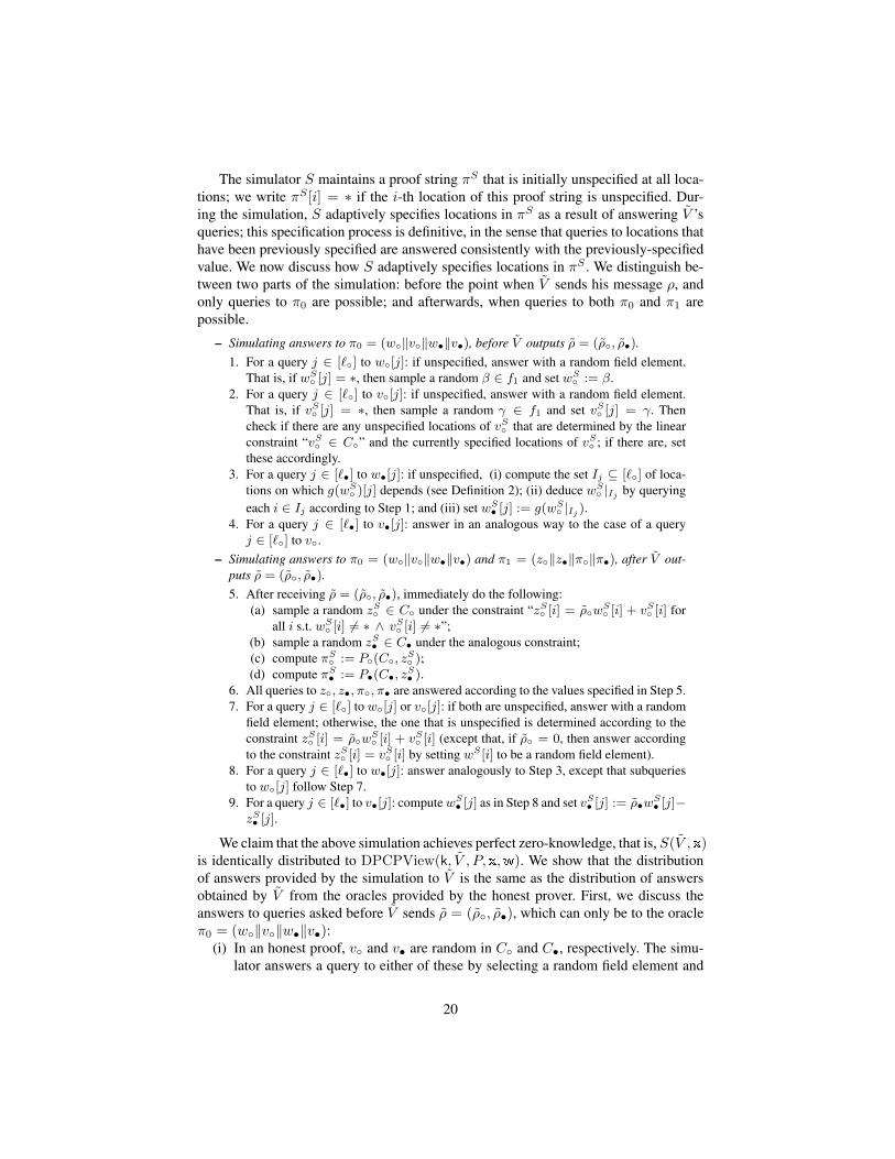
The simulator S maintains a proof string πS that is initially unspecified at all loca-tions; we write πS [i] = ∗ if the i-th location of this proof string is unspecified. Dur-ing the simulation, S adaptively specifies locations in πS as a result of answering V ’squeries; this specification process is definitive, in the sense that queries to locations thathave been previously specified are answered consistently with the previously-specifiedvalue. We now discuss how S adaptively specifies locations in πS . We distinguish be-tween two parts of the simulation: before the point when V sends his message ρ, andonly queries to π0 are possible; and afterwards, when queries to both π0 and π1 arepossible.

– Simulating answers to π0 = (w‖v‖w•‖v•), before V outputs ρ = (ρ, ρ•).1. For a query j ∈ [`] to w[j]: if unspecified, answer with a random field element.

That is, if wS [j] = ∗, then sample a random β ∈ f1 and set wS

:= β.2. For a query j ∈ [`] to v[j]: if unspecified, answer with a random field element.

That is, if vS [j] = ∗, then sample a random γ ∈ f1 and set vS [j] = γ. Thencheck if there are any unspecified locations of vS that are determined by the linearconstraint “vS ∈ C” and the currently specified locations of vS ; if there are, setthese accordingly.

3. For a query j ∈ [`•] to w•[j]: if unspecified, (i) compute the set Ij ⊆ [`] of loca-tions on which g(wS

)[j] depends (see Definition 2); (ii) deduce wS |Ij by querying

each i ∈ Ij according to Step 1; and (iii) set wS• [j] := g(wS

|Ij ).4. For a query j ∈ [`•] to v•[j]: answer in an analogous way to the case of a queryj ∈ [`] to v.

– Simulating answers to π0 = (w‖v‖w•‖v•) and π1 = (z‖z•‖π‖π•), after V out-puts ρ = (ρ, ρ•).5. After receiving ρ = (ρ, ρ•), immediately do the following:

(a) sample a random zS ∈ C under the constraint “zS [i] = ρwS [i] + vS [i] for

all i s.t. wS [i] 6= ∗ ∧ vS [i] 6= ∗”;

(b) sample a random zS• ∈ C• under the analogous constraint;(c) compute πS

:= P(C, zS );

(d) compute πS• := P•(C•, z

S• ).

6. All queries to z, z•, π, π• are answered according to the values specified in Step 5.7. For a query j ∈ [`] to w[j] or v[j]: if both are unspecified, answer with a random

field element; otherwise, the one that is unspecified is determined according to theconstraint zS [i] = ρw

S [i] + vS [i] (except that, if ρ = 0, then answer according

to the constraint zS [i] = vS [i] by setting wS [i] to be a random field element).8. For a query j ∈ [`•] to w•[j]: answer analogously to Step 3, except that subqueries

to w[j] follow Step 7.9. For a query j ∈ [`•] to v•[j]: computewS

• [j] as in Step 8 and set vS• [j] := ρ•wS• [j]−

zS• [j].

We claim that the above simulation achieves perfect zero-knowledge, that is, S(V , x)is identically distributed to DPCPView(k, V , P, x,w). We show that the distributionof answers provided by the simulation to V is the same as the distribution of answersobtained by V from the oracles provided by the honest prover. First, we discuss theanswers to queries asked before V sends ρ = (ρ, ρ•), which can only be to the oracleπ0 = (w‖v‖w•‖v•):

(i) In an honest proof, v and v• are random in C and C•, respectively. The simu-lator answers a query to either of these by selecting a random field element and

20

then propagating to other locations the linear constraints imposed by belongingto the linear code.

(ii) In an honest proof, w is computed as w := u′ + α, where u′ is random inC ′. Any t values from a random codeword in C ′ are distributed identically tot random field elements, because C ′ is t-wise independent. The queries of Vdetermine at most k · q = t locations of w. Hence, in an honest proof, V getsuniformly random answers for its queries to w; this matches the simulated viewwhere S answers V ’s queries to w with random fields elements.

(iii) In an honest proof, w• is a deterministic function of w: w• := g(w). As de-scribed above, the ≤ t positions of w determined by the verifier’s questions areuniformly random in the honest proof, as well as in the simulated proof. Thereforethe honest and the simulated views of w• are identically distributed, as determin-istic functions of identically distributed random variables.

Next, we discuss the answers to queries asked after V sends ρ = (ρ, ρ•); now V canquery both π0 = (w‖v‖w•‖v•) and π1 = (z‖z•‖π‖π•).

In an honest proof, answers to verifiers queries after sending ρ are from an uniformdistribution of v ∈ C, v• ∈ C•, u

′ ∈ C ′ (and deterministic functions of those andα), that is further conditioned on the answers given before sending ρ.

We conclude the discussion of the simulator by examining the time complexity ofthe simulation. Most steps of the simulation require (a) sampling a random field ele-ment and, possibly, (b) solving a linear system with a polynomial number of equations.The only expensive part of the simulation is Step 5, because it requires sampling randomcodewords in C and C•, as well as computing PCPP proofs for these two codewords.Provided that r1 is polynomially bounded, the entire simulation also runs in polynomialtime in the instance size n. (The definition of zero knowledge in Section 3 prescribes,as typically done, a simulator that runs in expected probabilistic polynomial time; oursimulator runs in strict probabilistic polynomial time.)

7 From NTIME to randomizable linear algebraic CSPs

– RAP & RGAP. In Section 7.1, we define algebraic problems, implicit in several in-fluential works on PCPs and IP [5, 30, 4, 2] and explicitly defined in [34, 37, 22].Afterward, we define group-preserving algebraic problems, a new “symmetric” vari-ant of algebraic problems that not only are powerful enough to efficiently captureNTIME but are also naturally “randomizable”, as discussed below.

– RAP → RLA. In Section 7.2 (see Lemma 2), we show that algebraic problems are asublanguage of linear algebraic CSPs. This observation shows that the techniques ofthis paper could potentially be applied to many PCP systems (e.g., those in [5, 30, 4,2, 37, 22, 13, 14, 15, 11, 16] to name a few) and also provides a “warm up” for thenext item.

– RGAP → RRLA. In Section 7.3 (see Lemma 3), we show an efficient reduction fromgroup-preserving algebraic problems to randomizable linear algebraic CSPs. In otherwords, the property of group preservation allows the corresponding linear algebraicCSPs to be randomizable.

– NTIME→ RGAP. In Section 7.4 (see Lemma 4), we show an efficient reductionfrom NTIME to group-preserving algebraic problems.

21

– NTIME→ RRLA. In Section 7.5 (see Theorem 6), we explain how to combinethe above to obtain the efficient reduction from NTIME to randomizable linearalgebraic CSPs.

7.1 Algebraic problems and group preservation

The definition below of algebraic problems is essentially due to [34] (though the term“algebraic problem” is from [22]); variants of it appear in later works such as [36, 37,22, 15, 14, 10, 16].

Definition 6 (RAP). Given functions F : N→ F , and h,m, η, d, σ : N→ N, the rela-tion

RAP[F, h,m, η, d, σ]

consists of instance-witness pairs (x,w) satisfying the following.

– The instance x is a tuple (1n, H,Q,N) where:• H is a subset of F (n) with cardinality h(n);• Q is a polynomial in F (n)[X1, . . . , Xm(n), Y1, . . . , Yη(n)] such that (i) it has

degree less than h(n) in each variable Xi, (ii) it has total degree at most d(n)when viewed as a polynomial in the variables Y1, . . . , Yη(n) with coefficients inF (n)[X1, . . . , Xm(n)], (iii) it can be evaluated by an arithmetic circuit of sizeσ(n);

• N = (N1, . . . , Nη(n)) and each Ni : F (n)m(n) → F (n)m(n) is an invertible

affine function.– The witness w is a polynomial A in F (n)[X1, . . . , Xm(n)].– The instance x and witness w jointly satisfy the following:

for every α ∈ Hm(n), (Q A N)(α) = 0 (1)

where

(QAN)(X) := Q(X1, . . . , Xm(n), A(N1(X1, . . . , Xm(n))), . . . , A(Nη(n)(X1, . . . , Xm(n)))) .(2)

Next, we define group-preserving algebraic problems, a family of algebraic prob-lems in which the set H is a subgroup of F (n) and the neighbor functions act on theproduct group Hm(n). The additional symmetry enables a reduction to randomizablelinear algebraic CSPs, which give rise to zero knowledge duplex PCPs. We believe thatgroup-preserving algebraic problems may find applications in the study of PCPs beyondtheir use in this paper.

Definition 7 (RGAP). The relation RGAP[F, h,m, η, d, σ] is the sub-relation of RAP[F, h,m, η, d, σ]obtained via restriction to instances that are group preserving. An instance x = (1n, H,Q,N)is group preserving if: (i) H is an additive or a multiplicative subgroup of F (n);(ii) each Ni : F (n)m(n) → F (n)m(n) in N can be identified with an element χi inHm(n) such that Ni(x) = χi x, where denotes the group operation of the productgroup Hm(n).

22

We also write RGAP[F, h,m, η, d, σ,+] to denote the further restriction to instancesthat are additively group preserving (i.e., H is an additive subgroup); similarly, wewrite RGAP[F, h,m, η, d, σ,×] to denote the the restriction to instances that are multi-plicatively group preserving.

– The degree of x, denoted |x|deg, is degY1,...,Yη(n)(Q), i.e., the total degree of Q

viewed as a polynomial in the variables Y1, . . . , Yη(n) with coefficients in the ringF[X1, . . . , Xm(n)].

– The circuit size of x, denoted |x|circ, is the circuit size of Q.

7.2 Algebraic problems naturally reduce to linear algebraic CSPs

Lemma 2 (RAP → RLA). For every F : N → F , h,m, η, d, σ : N → N, ε : N →(0, 1), and R ⊆ RAP[F, h,m, η, d, σ] there exist a relation R′ and algorithms inst,wit1,wit2satisfying the following conditions:

– EFFICIENT REDUCTION. For every instance x, letting x′ := inst(x):• for every witness w, if (x,w) ∈ R then (x′,wit1(x,w)) ∈ R′;• for every witness w′, if (x′,w′) ∈ R′ then (x,wit2(x,w

′)) ∈ R.Moreover, inst runs in time poly(|x|), wit1 in time poly(|x|) · O(|w| · η ·σ), and wit2in time poly(|x|) · O(|w′|).

– LINEAR ALGEBRAIC CSP. The relation R′ is a subset of

RLA

f = F` = |F |mρ = ( hd|F | )

m

δ = 1− hd|F |

q = ηc = σ + ηγ = ηεε

.

– RM CODES. If x = (1n, H,Q,N) then inst(x) = (1n, C, C•, g) with

• C = RM[F (n), F (n),m(n), h(n)

|F (n)|

];

• C• = VRM[F (n), F (n),m(n), h(n)d(n)|F (n)| , H

];

• g is the function that maps F (n)[X1, . . . , Xm(n)] to F (n)F (n)m(n)

as follows:given A in F (n)[X1, . . . , Xm(n)] and ω ∈ F (n)m(n), the ω-th coordinate of g(A)equals to (Q A N)(ω).

Proof (Proof of Lemma 2). Let x = (1n, H,Q,N) be an instance of RAP[F, h,m, η, d, σ],and construct x′ := inst(x) = (1n, C, C•, g) as above. We first argue that x′ is an in-stance of RLA[f, `, ρ, δ, q, c, γ, ε].

First, C and C• are linear error correcting codes with block length at most ` :=|F |m, rate at most ρ := max( h

|F | )m, ( hd|F | )

m, and relative distance at least δ :=

min1− h|F | , 1−

hd|F | over the same field F . (See Section 2.4.)

23

By construction, the function g is q-local with q := η and c-efficient with c := σ+η;moreover, g is (γ, ε)-sampling with γ := ηε, as we now explain. (See Definition 1 fordefinitions of these properties.) For every ω ∈ Fm, Iω denotes the set of indices in Fm

that g(·)[ω] depends on; for the g above, Iω equals N1(ω), . . . , Nη(ω). For everyω′ ∈ Fm and ω ∈ Fm, if ω′ ∈ Iω then ω ∈ N−11 (ω′), . . . , N−1η (ω′). Hence, thenumber of ω’s with ω′ ∈ Iω is at most η, because each Ni is invertible. We deduce thatPr[ Iω ∩ I 6= ∅ |ω ← Fm ] ≤ (η · |I|) /|F |m ≤ ηε.

Finally,C•∪g(C) has relative distance at least δ because it is a subset of RM[F, F,m, hd|F | ].This claim is immediate forC•; for g(C), it follows from the fact thatQAN has, ineach variable, a degree that is at most a multiplicative factor of d larger than the degreeof A.

We conclude the proof by explaining how one obtains the two witness maps wit1,wit2.For wit1, suppose that w = A ∈ F [X1, . . . , Xm] is a witness for x; then one can ver-ify that w′ := (α, α•), where α := A and α• := Q A N , is a witness for x′;α• can be efficiently obtained by first computing the evaluation of A on Fm (via anFFT), then computing the evaluation of Q A N on Fm (via point-to-point computa-tion), and finally interpolating (via an inverse FFT). Conversely, for wit2, suppose thatw′ = (α, α•) is a witness for x′; then one can verify that w := α is a witness for x.

7.3 From group-preserving algebraic problems to randomizable linear algebraicCSPs

Lemma 3 (RGAP → RRLA). For everyF : N→ F , h,m, η, d, σ, t : N→ N, δ, ε : N→(0, 1) with |F | ≥ h, where h denotes the smallest integral multiple of h that is greaterthan (h+t)d

1−δ , and for any R ⊆ RGAP[F, h,m, η, d, σ] there exist a relation R′ andalgorithms inst,wit1,wit2 satisfying the following conditions:

– EFFICIENT REDUCTION. For every instance x, letting x′ := inst(x):• for every witness w, if (x,w) ∈ R then (x′,wit1(x,w)) ∈ R′;• for every witness w′, if (x′,w′) ∈ R′ then (x,wit2(x,w

′)) ∈ R.Moreover, inst runs in time poly(|x|), wit1 in time poly(|x|) · O(|w| · η ·σ), and wit2in time poly(|x|) · O(|w′|).

– RANDOMIZABLE LINEAR ALGEBRAIC CSP. The relation R′ is a subset of

RRLA

f = F

` = hm

ρ = ( (h+t)dh

)m

δ = 1− ( (h+t)dh

)

q = ηc = σ + ηγ = ηεεt

r = O(hm)

.

24

Proof (Proof of Lemma 3). Let x = (1n, H,Q,N) be an instance of RGAP[F, h,m, η, d, σ].We construct an instance x′ := inst(x) = (1n, C, C•, g) of RRLA[f, `, ρ, δ, q, c, γ, ε, t, r]as follows.

Let H be a subset of F that is a union of cosets of H with |H| = h and H ∩H = ∅.(This can be done as follows: let S be a subset of the quotient group F/H withcardinality |S| = h/h that does not include 1, where F denotes the additive ormultiplicative group of F , depending on whether H is additive or multiplicative, and1 is the identity in H; then set H := x y |x ∈ S, y ∈ H.) Analogously to theproof of Lemma 2, we define:– C := RM

[F (n), H,m(n), h(n)+t(n)

h(n)

];

– C• := VRM[F (n), H,m(n), (h(n)+t(n))d(n)

h(n), H];

– g to be the function that maps F (n)[X1, . . . , Xm(n)] to F (n)Hm(n)

as follows: givenA in F (n)[X1, . . . , Xm(n)] and ω ∈ Hm(n), the ω-th coordinate of g(A) equals to(Q A N)(ω). Note that g is well-defined, i.e., g(A) is a function from Hm(n) toF (n); this follows from the group preservation property of x (see Definition 7): forevery ω ∈ Hm and i ∈ [η], it holds thatNi(ω) ⊆ Hm because H is a union of cosetsof H and Ni multiplies every coordinate of ω by an element of H .

We first argue that x′ constructed above is an instance of RRLA[f, `, ρ, δ, q, c, γ, ε, t, r].First, analogously to the proof of Lemma 2, we note that C and C• are linear error

correcting codes with block length at most ` := hm, rate at most ρ := max(h+th

)m, ( (h+t)dh

)m,and relative distance at least δ := min1− h+t

h, 1− (h+t)d

h over the same field F ; also,

we deduce that g is q-local with q := η, c-efficient with c := σ+η, and (γ, ε)-samplingwith γ := ηε.

Next, recalling Definition 5, x′ is t-randomizable in time r := O(hm) because:(i) C ′ := VRM[F (n), H,m, h+t

h, H] is a subcode of C and it is t-wise independent

due to Claim 2.4 (C ′ satisfies the hypotheses becauseH∩H = ∅ and h−h ≥ (h+t)d1−δ −

h ≥ t); and (ii) one can sample random elements from C ′, C and C• in time O(hm)by using the the quasilinear FFT algorithms for multipoint evaluation and interpolation(sampling the random polynomial in necessary basis is easy forC; for vanishing Reed–Muller codes we rely on Alon’s Combinatorial Nullstelensatz [1] as per Lemma 4.11 of[15]).

We conclude the proof by observing that necessary witness maps wit1,wit2 ex-ist. Just as in Lemma 2, if w = A ∈ F (n)[X1, . . . , Xm(n)] is a witness for x thenwit1(x,w) outputs w′ := (A,Q A N), which is a witness for x′; conversely, ifw′ = (α, α•) is a witness for x′ then wit2(x,w

′) outputs w := α, which is a witnessfor x.

7.4 An efficient reduction from NTIME to group-preserving algebraicproblems

The following lemma gives an efficient reduction from NTIME to group-preservingalgebraic problems in which instances are over fields of characteristic 2 and preserveadditive groups.

25

Lemma 4 (NTIME→ RGAP). For every h,m, T : N→ N with h(n)m(n) = Ω(T (n) log T (n))and R ∈ NTIME(T ) there exist a relation R′ and algorithms inst,wit1,wit2 satisfy-ing the following conditions:

– EFFICIENT REDUCTION. For every instance x, letting x′ := inst(x):• for every witness w, if (x,w) ∈ R then (x′,wit1(x,w)) ∈ R′;• for every witness w′, if (x′,w′) ∈ R′ then (x,wit2(x,w

′)) ∈ R.Moreover, inst runs in time poly(n + log h(n) +m(n)) and wit1,wit2 run in timeO(T (n)).

– GROUP PRESERVING ALGEBRAIC PROBLEM. The relation R′ is a subset of

RGAP

F = F2log T+O(log log T )

hmη = polylog(T )d = O(1)σ = poly(n+ log T )+

.

The proof appears in the full version.

7.5 Combining the two reductions

By combining Lemma 4 and Lemma 3, we obtain the following theorem, which givesthe reduction claimed at the beginning of this section.

Theorem 6 (NTIME → RRLA). For every T, t : N → N, δ, ε : N → (0, 1), andR ∈ NTIME(T ) there exist a relation R′ and algorithms inst,wit1,wit2 satisfyingthe following conditions:

– EFFICIENT REDUCTION. For every instance x, letting x′ := inst(x):• for every witness w, if (x,w) ∈ R then (x′,wit1(x,w)) ∈ R′;• for every witness w′, if (x′,w′) ∈ R′ then (x,wit2(x,w

′)) ∈ R.Moreover, inst runs in time poly(n + log(T (n)+t(n)

1−δ(n) )) and wit1,wit2 run in time

poly(n) · O(T (n)+t(n)1−δ(n) ).

– RANDOMIZABLE LINEAR ALGEBRAIC CSP. The relation R′ is a subset of

RRLA

f = F2log(T+t)+O(log log(T+t))

` = O(T+t1−δ )

ρ = 1− δδq = polylog(T )c = poly(n+ log T )γ = polylog(T ) · εεt

r = O(T+t1−δ )

.

26

– AFFINE RS CODES OVER CHARACTERISTIC 2. Both CR′, and CR′,• are subsetsofRS∗ρ ∪ VRS

∗ρ (see Section 2.4).

Proof (Proof of Theorem 6). First, we invoke Lemma 4 with h,m, T such that m(n) =

1 and h(n) = O(T (n) log T (n)); this yields a relation R(1) and algorithms inst(1),wit(1)1 ,wit(1)2

such that: (i) inst(1),wit(1)1 ,wit(1)2 provide a reduction from R ∈ NTIME(T ) to R(1),

with inst(1)(x) running in time poly(n+log h(n)+m(n)) and wit(1)1 (x,w),wit

(1)2 (x,w(1))

in time O(T (n)); and (ii) R(1) is a subset of

RGAP

F = F2log T+O(log log T )

h = O(T (n) log T (n))m = 1η = polylog(T )d = O(1)σ = poly(n+ log T )+

.

Next, we invoke Lemma 3 on R(1), using δ, ε, t from the theorem statement. Notethat the conditions of the theorem are satisfied as |F | ≥ (h+t)d

1−δ +h ≥ h . Therefore this

yields a relation R(2) and algorithms inst(2),wit(2)1 ,wit(2)2 such that: (i) inst(2),wit(2)1 ,wit

(2)2

provide a reduction from R(1) to R(2), with inst(2)(x(1)) running in time poly(|x(1)|),wit

(2)1 (x(1),w(1)) in time poly(|x(1)|) · O(|w(1)| · η · σ) and wit

(2)2 (x(1),w(2)) in time

poly(|x(1)|) · O(|w(2)|); and (ii) R(2) is a subset of

RRLA

f = F` = O(h+t1−δ )

ρ = 1− δδq = ηc = σ + ηγ = ηεεt

r = O(h+t1−δ )

.

One can check that R(2) achieves the parameters specified in the theorem statement.The desired reduction from R to R(2) is given by the algorithms inst(x) := inst(2)(inst(1)(x)),

wit1(x,w) := wit(2)1 (inst(1)(x),wit

(1)1 (x,w)), and wit2(x,w

′) := wit(1)2 (x,wit

(2)2 (inst(1)(x),w′)).

One can verify that inst runs in time poly(n + log(T (n)+t(n)1−δ(n) )) and wit1,wit2 run in

time poly(n) · O(T (n)+t(n)1−δ(n) ).

8 Proof of Theorem 4

Proof (Proof of Theorem 4). We explain how to combine 6 and Lemma 5 (and Theo-rem 3) so to obtain Theorem 4.

27

Let R be a relation in NTIME(T ); we need to construct a duplex PCP system forR with the claimed parameters. For now we focus on achieving soundness of 1

2 , anddiscuss the general case at the end of the proof.a

We first reduce NTIME to randomizable linear algebraic CSPs: invoke Theorem 6on R to obtain a relation R′ and algorithms inst,wit1,wit2 such that: (i) inst,wit1,wit2provide a reduction from R to R′, with inst running in time poly(n + log(T (n) +t1(n))) and wit1,wit2 in time O(T (n) + t1(n)); and (ii) R′ is a subset of

RRLA

f1 = F2log(T+t1)+O(log log(T+t1))

`1 = O(T + t1)ρ1 = 1− δ1δ1q1 = polylog(T )c1 = poly(n+ log T )γ1 = polylog(T ) · ε1ε1t1r1 = O(T+t1

1−δ1 )

.

Above, as parameters of Theorem 6, we chose ε1, δ1 and t1 as follows: ε1 such thatγ1 = polylog(T ) · ε1 ≤ 2

9 , then δ1 := 1− ε1/4, and t1 := k · q1 = k · polylog(T ).

Next we obtain PCPP systems for the relations corresponding to codes appearingin instances of R′. Theorem 6 guarantees that both CR′, and CR′,• are subsets ofRS∗ρ ∪VRS

∗ρ. We now invoke Theorem 3, choosing λ = 2 and s such that fields f1 for

R′ and a2 for the PCPPs match. That is, we chose s = O(log log(T + t1)) and obtain:

Rel(CR′,) , Rel(CR′,•) ∈ PCPP

a2 = F2s+log `1

l2 = O(`1)q2 = polylog(`1)∆2 = ∆Ham

a

d2 = ρ1/2e2 = 1/4

tp2 = poly(s) · O(`1)tv2 = poly(s+ log `1)na

.

Finally we invoke Theorem 5 for R′ to obtain a duplex PCP system for R′, supply-ing the PCPPs we just obtained from Theorem 3. Note that our choices satisfy the hy-pothesis of Theorem 5 is satisfied, as the two fields match, r1 is polynomially bounded,and as we chose γ1, ε1 ≤ 2

9 , δ1 ≥ 1718 , we also have ε1 < min δ12 , δ1 − γ1 and

28

d2 ≤ ε1/4. This establishes our claim that:

R ∈ DPCPpzk

a = F2log(T+t1)+O(log log(T+t1))

l = 2l2(`1) + 6`1 = O(T + t1)q = 2q2(`1) + q1 + 7 = polylog(T )e = 1

2

tp = inst+ wit1 + (2tp2(`1) + (c1 + 5)`1 + r1) = poly(n) · O(T + k)tv = inst+ (2tv2(`1) + c1 + log `1) = poly(n+ log(T + k))kna

.

The precise expression for soundness error is e := max1−δ1+γ1+ε1 , (1−|f1|−1) ·maxe2, ε1/4+ |f1|−1, but it is upper bounded by 1

2 , as for us 1− δ1+ γ1+ ε1 ≤ 12 ,

maxe2, ε1/4 = 14 and |f1| ≥ 4.

Acknowledgments

We thank Yuval Ishai and Mor Weiss for helpful discussions. The research leading tothese results has received funding from: the European Community’s Seventh Frame-work Programme (FP7/2007-2013) under grant agreement number 240258; the IsraeliScience Foundation (grant 1501/14); and the Center for Science of Information (CSoI),an NSF Science and Technology Center, under grant agreement CCF-0939370.

References

1. Alon, N.: Combinatorial Nullstellensatz. Comb. Probab. Comput. (1999)2. Arora, S., Lund, C., Motwani, R., Sudan, M., Szegedy, M.: Proof verification and the hard-

ness of approximation problems. JACM (1998)3. Arora, S., Safra, S.: Probabilistic checking of proofs: a new characterization of NP. JACM

(1998)4. Babai, L., Fortnow, L., Levin, L.A., Szegedy, M.: Checking computations in polylogarithmic

time. In: STOC ’91 (1991)5. Babai, L., Fortnow, L., Lund, C.: Non-deterministic exponential time has two-prover inter-

active protocols. Computational Complexity (1991)6. Babai, L., Moran, S.: Arthur-Merlin games: a randomized proof system, and a hierarchy of

complexity class. Journal of Computer and System Sciences (1988)7. Bellare, M., Goldreich, O.: On defining proofs of knowledge. In: CRYPTO ’92 (1993)8. Ben-Or, M., Goldreich, O., Goldwasser, S., Hastad, J., Kilian, J., Micali, S., Rogaway, P.:

Everything provable is provable in zero-knowledge. In: CRYPTO ’88 (1988)9. Ben-Or, M., Goldwasser, S., Kilian, J., Wigderson, A.: Multi-prover interactive proofs: how

to remove intractability assumptions. In: STOC ’88 (1988)10. Ben-Sasson, E., Chiesa, A., Genkin, D., Tromer, E.: Fast reductions from RAMs to delegat-

able succinct constraint satisfaction problems. In: ITCS ’13 (2013)11. Ben-Sasson, E., Chiesa, A., Genkin, D., Tromer, E.: On the concrete efficiency of

probabilistically-checkable proofs. In: STOC ’13 (2013)12. Ben-Sasson, E., Goldreich, O., Harsha, P., Sudan, M., Vadhan, S.: Robust PCPs of proximity,

shorter PCPs and applications to coding. In: STOC ’04 (2004)

29

13. Ben-Sasson, E., Goldreich, O., Harsha, P., Sudan, M., Vadhan, S.: Short PCPs verifiable inpolylogarithmic time. In: CCC ’05 (2005)

14. Ben-Sasson, E., Goldreich, O., Harsha, P., Sudan, M., Vadhan, S.: Robust PCPs of proximity,shorter PCPs, and applications to coding. SIAM J. Comp. (2006)

15. Ben-Sasson, E., Sudan, M.: Short PCPs with polylog query complexity. SIAM J. Comp.(2008)

16. Ben-Sasson, E., Viola, E.: Short PCPs with projection queries. In: ICALP ’14 (2014)17. Dinur, I.: The PCP theorem by gap amplification. JACM (2007)18. Dinur, I., Reingold, O.: Assignment testers: Towards a combinatorial proof of the PCP theo-

rem. In: FOCS ’04 (2004)19. Dwork, C., Feige, U., Kilian, J., Naor, M., Safra, S.: Low communication 2-prover zero-

knowledge proofs for NP. In: CRYPTO ’92 (1992)20. Goldwasser, S., Micali, S., Rackoff, C.: The knowledge complexity of interactive proof-

systems. In: STOC ’85 (1985)21. Goyal, V., Ishai, Y., Mahmoody, M., Sahai, A.: Interactive locking, zero-knowledge PCPs,

and unconditional cryptography. In: CRYPTO ’10 (2010)22. Harsha, P., Sudan, M.: Small PCPs with low query complexity. Computational Complexity

(2000)23. Impagliazzo, R., Yung, M.: Direct minimum-knowledge computations. In: CRYPTO ’87

(1987)24. Ishai, Y., Kushilevitz, E., Ostrovsky, R., Sahai, A.: Zero-knowledge proofs from secure mul-

tiparty computation. SIAM J. Comput. (2009)25. Ishai, Y., Mahmoody, M., Sahai, A.: On efficient zero-knowledge PCPs. In: TCC ’12 (2012)26. Ishai, Y., Mahmoody, M., Sahai, A., Xiao, D.: On zero-knowledge PCPs: Limitations, sim-

plifications, and applications (2015), available at http://www.cs.virginia.edu/˜mohammad/files/papers/ZKPCPs-Full.pdf

27. Kalai, Y.T., Raz, R.: Interactive PCP. In: ICALP ’08 (2008)28. Kilian, J., Petrank, E., Tardos, G.: Probabilistically checkable proofs with zero knowledge.

In: STOC ’97 (1997)29. Lapidot, D., Shamir, A.: A one-round, two-prover, zero-knowledge protocol for NP. Combi-

natorica (1995)30. Lund, C., Fortnow, L., Karloff, H., Noam, N.: Algebraic methods for interactive proof sys-

tems. JACM (1992)31. Mahmoody, M., Xiao, D.: Languages with efficient zero-knowledge pcps are in SZK. In:

TCC ’13 (2013)32. Mie, T.: Polylogarithmic two-round argument systems. Journal of Mathematical Cryptology

(2008)33. Ostrovsky, R., Wigderson, A.: One-way functions are essential for non-trivial zero-

knowledge. In: ISTCS ’93 (1993)34. Polishchuk, A., Spielman, D.A.: Nearly-linear size holographic proofs. In: STOC ’94 (1994)35. Shamir, A.: IP = PSPACE. JACM (1992)36. Spielman, D.: Computationally Efficient Error-Correcting Codes and Holographic Proofs.

Ph.D. thesis, Massachusetts Institute of Technology (1995)37. Szegedy, M.: Many-valued logics and holographic proofs. In: ICALP ’99 (1999)

30