![Title Fault-Tolerant Quantum Computation on Logical Cluster ......quantum computation under imperfect gate operations, namely fault-tolerant quantum computation [11, 12]. The main](https://static.fdocuments.net/doc/165x107/60f3fd58ff2b1f2547000d7a/title-fault-tolerant-quantum-computation-on-logical-cluster-quantum-computation.jpg)
Quantum Computation The theory of quantum computation, a new and promising eld, is discussed. The...
82
Quantum Computation Nicholas T. Ouellette March 18, 2002
Transcript of Quantum Computation The theory of quantum computation, a new and promising eld, is discussed. The...

Quantum Computation
Nicholas T. Ouellette
March 18, 2002

Abstract
The theory of quantum computation, a new and promising field, is discussed. Themathematical background to the field is presented, drawing ideas both from quan-tum mechanics and the theory of classical computation. The quantum circuitmodel of computation is discussed, and a universal set of quantum logic gates isinvestigated. Quantum algorithms are examined, focusing particularly on Grover’sdatabase search algorithm and Shor’s factoring algorithm, the two best known quan-tum algorithms. Finally, an implementation of quantum computation using linearoptics is developed.

Contents
1 Introduction 3
2 Mathematical Tools 6
2.1 Quantum Mechanics . . . . . . . . . . . . . . . . . . . . . . . . . . . 62.1.1 States and Qubits . . . . . . . . . . . . . . . . . . . . . . . . 62.1.2 Operators and Evolution . . . . . . . . . . . . . . . . . . . . . 72.1.3 Composite States and Registers . . . . . . . . . . . . . . . . . 8
2.2 The Theory of Computation . . . . . . . . . . . . . . . . . . . . . . . 102.2.1 Classical Turing Machines . . . . . . . . . . . . . . . . . . . . 102.2.2 Quantum Turing Machines . . . . . . . . . . . . . . . . . . . 122.2.3 Computational Complexity . . . . . . . . . . . . . . . . . . . 13
3 Quantum Gates and Circuits 14
3.1 Quantum Logic . . . . . . . . . . . . . . . . . . . . . . . . . . . . . . 143.2 Single Qubit Gates . . . . . . . . . . . . . . . . . . . . . . . . . . . . 153.3 Controlled Operations . . . . . . . . . . . . . . . . . . . . . . . . . . 203.4 Universal Gate Sets . . . . . . . . . . . . . . . . . . . . . . . . . . . 22
3.4.1 Two-Level Unitary Matrices . . . . . . . . . . . . . . . . . . . 233.4.2 Single Qubit and Control-NOT Gates . . . . . . . . . . . . . 263.4.3 A Discrete Universal Set . . . . . . . . . . . . . . . . . . . . . 28
4 Quantum Algorithms 30
4.1 Introduction . . . . . . . . . . . . . . . . . . . . . . . . . . . . . . . . 304.2 Deutsch’s Algorithm . . . . . . . . . . . . . . . . . . . . . . . . . . . 304.3 The Deutsch-Jozsa Algorithm . . . . . . . . . . . . . . . . . . . . . . 334.4 Grover’s Algorithm . . . . . . . . . . . . . . . . . . . . . . . . . . . . 35
4.4.1 Procedure . . . . . . . . . . . . . . . . . . . . . . . . . . . . . 354.4.2 Inversion about the Mean . . . . . . . . . . . . . . . . . . . . 364.4.3 An Alternate Approach . . . . . . . . . . . . . . . . . . . . . 40
4.5 Shor’s Algorithm . . . . . . . . . . . . . . . . . . . . . . . . . . . . . 434.5.1 Number Theoretic Background . . . . . . . . . . . . . . . . . 434.5.2 Order Finding . . . . . . . . . . . . . . . . . . . . . . . . . . 454.5.3 An Example: Factoring 15 . . . . . . . . . . . . . . . . . . . . 48
5 Linear Optics Quantum Computation 50
5.1 Why Linear Optics? . . . . . . . . . . . . . . . . . . . . . . . . . . . 505.2 Optical Realizations of Universal Quantum Logic Gates . . . . . . . 50
5.2.1 Spatial Mode Gates . . . . . . . . . . . . . . . . . . . . . . . 515.2.2 Polarization State Gates . . . . . . . . . . . . . . . . . . . . . 55
5.3 The Fourier and Hadamard Transforms . . . . . . . . . . . . . . . . 585.4 Some Simplifications . . . . . . . . . . . . . . . . . . . . . . . . . . . 615.5 Sample Optical Quantum Circuits . . . . . . . . . . . . . . . . . . . 62

5.5.1 Two-Qubit Circuit . . . . . . . . . . . . . . . . . . . . . . . . 625.5.2 n-Qubit Extension . . . . . . . . . . . . . . . . . . . . . . . . 64
6 Conclusion 66
Appendices 68
A Classical Logic Gates 68
B Classical Algorithms Used in Shor’s Algorithm 70
B.1 The Euclidean Algorithm for Greatest Common Divisors . . . . . . . 70B.2 Continued Fractions . . . . . . . . . . . . . . . . . . . . . . . . . . . 71
C Optical Quantum Nondemolition Measurements 75
Acknowledgements 79
References 79
2

1 Introduction
1 Introduction
The theory of quantum mechanics developed in the early part of the twentieth cen-tury is a theory of the very small. A very mathematical theory, it nevertheless makespredictions that agree to fantastic precision with experimentally determined results.In order to make the theory agree with the physical world, however, scientists havebeen forced to part with the determinism of classical physics in favor of proba-bilistic quantum mechanical predictions. This sacrifice of determinism has beenameliorated, however, by the identification of the quantum mechanical propertiesof superposition, interference, and entanglement as powerful resources. The theoryof quantum computation exploits these tools to perform computation exponentiallyfaster in some cases than is possible with any classical computer.
The theory of classical computation stands in stark contrast to quantum theory.It is not a theory describing the physical world; rather, it is purely mathematical,designed to provide a framework for studying algorithms. Much of computationaltheory is centered around the idea of the Turing machine, named after Alan Turing,the British mathematician who pioneered the field. A Turing machine is a simpletheoretical construct that has proved useful in studying computation, and one of thegreat triumphs of computer science has been to prove that there is no possible com-putation that cannot be performed on this simple apparatus. This idea is embodiedin the Church-Turing thesis, which states that the class of functions computable by aTuring machine is exactly the class of functions computable by algorithm [1]. Thus,the study of the theory of computation may be reduced to the study of the Turingmachine. While the full theory of Turing machines and computation is beyond thescope of this paper, we will on occasion make use of some of the concepts involved.
On the surface, then, it would appear that the fields of classical computation andquantum mechanics have no relation to one another. Indeed, the connection betweenthe two is subtle, and was not recognized until the 1980s. Appropriately enough,the first hints of this link grew out of information theory, a subject that also linkstogether abstract mathematical notions with the physical world. One fundamentalresult from information theory is Landauer’s Principle, which states that for everybit of information erased by a computing device, an amount of energy equal tokT ln 2 is released into the environment, where k is Boltzmann’s constant and T isthe temperature of the environment [2]. As heat dissipation is generally an unwantedside effect of computation, researchers began to study the possibility of computationwithout erasure. This led to the development of reversible computation, where everycomputation may be run backwards and thus loses no information. This result inturn led some scientists to wonder if quantum mechanical systems could be usedto compute, since quantum systems undergo unitary evolution, which is by its verynature reversible. Finally, in 1985, David Deutsch at Oxford University publisheda paper containing a full theory of a quantum Turing machine, making explicit thelink between computational theory and quantum mechanics [3].
Deutsch showed that the theory of computation developed by Turing and others
3

1 Introduction
is not free from physical assumptions. A classical Turing machine is assumed to bein a definite state at the conclusion of each step of computation. But a quantummechanical system is subject to no such constraint; the result of each step of thecomputation may be a superposition of computational states. Using this principle, aquantum Turing machine may, in a sense that will be explained more fully in Section4, explore all possible computational paths while performing only a single computa-tion. It is this principle of quantum parallelism that gives quantum computers theirpower. It is important to note at this point that a quantum Turing machine, andtherefore a quantum computer, is no more powerful than a classical Turing machine,in the sense that there is no function that may be computed by one that may notbe by the other. It appears, however, that quantum Turing machines may be ableto compute some functions more efficiently than classical Turing machines.
The two most famous and useful quantum algorithms known are Shor’s factoringalgorithm and Grover’s database search algorithm. Shor’s algorithm can factor num-bers faster than any known classical algorithm (though it has not yet been provedthat factoring is an inherently inefficient problem for a classical computer), whileGrover’s algorithm can speed up the search of an unstructured database by a factorof a square root of the number of elements in the database over the best classicalalgorithm. Both of these quantum algorithms, though especially Shor’s algorithm,have important applications to cryptography. The most widespread cryptosystemin use today is the RSA encryption scheme, which relies on the difficulty of fac-toring large numbers for its security. A quantum computer could decode an RSAencrypted message in seconds. Thus, research in quantum computation has alsospurred research in the related field of quantum cryptography, in which quantummechanical properties are used to create unbreakable codes.
Despite the obvious benefits of quantum computers, none yet exists. Manyphysical realizations have been proposed, but none has yet produced large quantumcomputers, even though the requirements for quantum computation seem minimal.Any quantum system possessing two nondegenerate states can be used as a quan-tum bit, or qubit, which is the basic unit of quantum information, just as the bitis the basic unit of classical information. A quantum computer would consist ofmany qubits and some mechanism for changing their state. Additionally, it must bepossible to entangle different qubits to create quantum registers; this notion will beexplained in a later section.
To date, only small quantum computers running a single algorithm have beenbuilt, despite the simple requirements. Though no solution has yet been found thatwill scale easily to large numbers of qubits, some implementations have been quitesuccessful on a small scale as proof-of-principle experiments. The most advanced ofthese small quantum computers are based on nuclear magnetic resonance (NMR). Inan NMR quantum computer, nuclear spins are used as qubits, and radio frequencywaves are used to change the state of the qubits. A simpler implementation, dis-cussed extensively in a later section of this paper, is based on linear optics, wherecombinations of photon spatial modes and polarization states are used as qubits.
4

1 Introduction
Experiments have also been done using quantum dots, cavity QED systems, andtrapped ions, to name a few. The reader is directed to Nielsen and Chuang’s book[1] for an overview of some of these implementations.
There are problems with each of these implementations, however, that havestymied the progress towards a working universal quantum computer. These prob-lems can be separated into implementation-specific issues and issues of general dif-ficulty. The most problematic of these general difficulties is decoherence, or thetendency of the delicate superpositions necessary for quantum computation to de-cay due to interactions with their environment. Several schemes have been devel-oped for dealing with this problem, most notably the theories of decoherence-freesubspaces and quantum error correcting codes. While these schemes do reduce theadverse effects caused by decoherence, they also require extra qubits that will slowthe development of working quantum computers.
In this paper, we present an overview of the field of quantum computation, alongwith a complete treatment of linear optical quantum computation as an exampleof a possible experimental realization of the theory. Section 2 develops the theoryof quantum mechanics from the viewpoint of quantum computation and introducessome useful ideas from the theory of computation. Section 3 gives an overviewof the quantum circuit model, and determines a set of quantum logic gates that isuniversal for quantum computation. Section 4 discusses several quantum algorithms,beginning with the relatively simple Deutsch and Deutsch-Jozsa algorithms and alsocovering Grover’s and Shor’s algorithms. Finally, Section 5 provides a completedescription of a hypothetical quantum computer implemented using linear optics.
5

2 Mathematical Tools
2 Mathematical Tools
2.1 Quantum Mechanics
The theory of quantum mechanics is built on top of the theory of linear algebra.In order to describe the physical world, we must define some mapping between themathematical concepts and observable physical dynamics. This is accomplished bydefining a set of postulates. We can say that the postulates are valid if the resultanttheory agrees with experiment, and indeed the predictions of quantum mechanicsagree impeccably with observations.
In this section, we develop the theory of quantum mechanics from the viewpointof quantum computation. The following discussion is adapted from Boccio [4] andNielsen and Chuang [1].
2.1.1 States and Qubits
To begin with, we must define a framework within which to work; to that end, wemake the following postulate:
Postulate 1 A physical system is represented as a Hilbert space, and a state of the
system is given by a unit vector |ψ〉 in that space. In particular, a qubit is a unit
vector in a two dimensional Hilbert space.
A Hilbert space is simply a complex linear vector space with an inner productdefined. Thus it is clear that linear algebra will be the primary mathematical for-malism used in our theory. In quantum computation, we are primarily interested inqubits; thus we will be most interested in simple two-dimensional vector spaces.
Qubits are the quantum analog of classical bits. As two dimensional vectors,they have two discrete states, which we label |0〉 and |1〉 . We also here define theso-called standard computational basis, in which
|0〉 =
(10
)
and |1〉 =
(01
)
. (2.1)
We will often make use of this basis, and unless otherwise stated, it is the basis usedthroughout this paper.
In addition to being in either of the basis states |0〉 or |1〉 , a qubit may exist inany superposition of these states, given by
|ψ〉 = α |0〉 + β |1〉 , (2.2)
with|α|2 + |β|2 = 1. (2.3)
The fact that qubits can be in definite superpositions is the root of the increasedcomputational power of quantum computers relative to classical computers.
6

2.1 Quantum Mechanics
2.1.2 Operators and Evolution
Now that we have developed a mathematical representation of a physical system andits states, we must specify how states evolve. We thus make our second postulate:
Postulate 2 Closed systems evolve via unitary transformations. Thus, quantum
logic gates, which change the state of qubits, are represented as unitary operators.
A unitary operator is one whose Hermitian conjugate is its inverse. Thus, if Uis a unitary operator,
U †U = UU † = I, (2.4)
where I is the identity operator. This allows us to state and prove a lemma con-cerning the eigenvalues of a unitary operator that we shall use later in this paper:
Lemma 2.1 A unitary operator has eigenvalues of the form eiθ, and any operator
with eigenvalues of this form is unitary.
Proof To prove the first part of the lemma, consider the matrix representationof a unitary operator in its eigenbasis. In this basis, it will be diagonal with itseigenvalues υi down the diagonal, where the υi are in general complex. The productU †U in this basis will then be a diagonal matrix with the values υ∗i υi down thediagonal. To fulfill the unitary condition, we must have υ∗i υi = 1; thus, the real partof the υi must be 1, and therefore the υi will be of the form eiθi . Examining theproduct UU † gives the same result.
The second part of the lemma is proved in much the same way. We definesome operator Q with eigenvalues eiφi , and work in its eigenbasis. In this basis,the product Q†Q has a matrix representation consisting of e−iφieiφi = 1 down thediagonal, and thus is the identity matrix. The same result is obtained given theproduct QQ†, and so Q fulfills the unitarity condition and the lemma is proved.
�
Notice that postulate 2 specifies only that closed systems undergo unitary evo-lution. No specification is made for systems that are not closed; presumably, thedynamics are far more complex. Many of the difficulties encountered in the effort toconstruct a working quantum computer stem from the interactions of the computerwith its environment; quantum computers are only approximately closed systems. Inthis paper, however, we consider only ideal, closed quantum computational systems,and so are concerned only with purely unitary evolution.
Postulate 2 associates the class of unitary operators with state evolution. Wenow associate a second class of operators with physical observables, which will leadus to a representation of quantum measurement:
Postulate 3 A physical dynamical variable is represented by a Hermitian operator,
and the possible outcomes of a measurement of that observable are the eigenvalues
of the operator.
7

2.1 Quantum Mechanics
A Hermitian operatorH is one that is equal to its Hermitian conjugate, satisfyingthe relation H = H†. Just as the unitarity condition restricts the eigenvalues of aunitary operator, the hermiticity condition imposes a restriction on the eigenvaluesof a Hermitian operator:
Lemma 2.2 The eigenvalues of a Hermitian operator are real.
Proof Consider a Hermitian operator H, and again consider its matrix representa-tion in its eigenbasis, where it is diagonal with its eigenvalues ηi down the diagonaland the ηi are in general complex. To satisfy the hermiticity condition, H = H †,the relation η = η∗ must hold. Thus, the ηi must be real.
�
The condition proved in lemma 2.2 makes Hermitian operators a good choice tomodel observables, since, of course, we can never measure a complex number.
As we show below, the eigenvectors of a Hermitian operator are orthogonal, afact we shall often use:
Theorem 2.1 The eigenvectors of a Hermitian operator corresponding to distinct
eigenvalues are orthogonal.
Proof Let Q be a Hermitian operator, and let |ψ〉 and |φ〉 be eigenvectors of Qwith eigenvalues ψ and φ, respectively, such that ψ 6= φ. The, we have
φ 〈ψ |φ〉 = 〈ψ |Q|φ〉 = (Q |ψ〉)† |φ〉 = (ψ |ψ〉)† |φ〉 = ψ 〈ψ |φ〉 , (2.5)
where the last equality follows from lemma 2.2. Therefore,
φ 〈ψ |φ〉 = ψ 〈ψ |φ〉 , (2.6)
and so 〈ψ |φ〉 = 0, which means that |ψ〉 and |φ〉 are orthogonal.
�
2.1.3 Composite States and Registers
So far in our discussion of quantum mechanics, we have dealt only with singlesystems; from the standpoint of quantum computation, we have only discussedsingle qubits. A quantum computer with the capacity to operate on only a singlequbit is useless, and so we must extend our discussion to systems of many qubits.We therefore introduce the following postulate:
Postulate 4 The Hilbert space describing a composite physical system is the tensor
product of the spaces describing the individual systems, and the state vector of the
system is the tensor product of the individual state vectors. A quantum register is
the tensor product of individual qubits.
8

2.1 Quantum Mechanics
The tensor product, denoted by the ⊗ operator, is associative and distributive.In terms of matrices and vectors, the tensor product is reduced to the so-calledKronecker product. The Kronecker product of an m × n matrix A and a p × qmatrix B is given by
A⊗B =
nq︷ ︸︸ ︷
A11B A12B · · · A1nBA21B A22B · · · A2nB
· · · · · · ... · · ·Am1B Am2B · · · AmnB
mp. (2.7)
In equation (2.7), each entry is a submatrix of the dimensions of B, with each entryin B multiplied by a component of A as shown. The Kronecker product of a vectorfollows directly from equation (2.7) by simply setting n and q to 1. Let us illustratethe tensor product with a simple example.
Consider the matrix
H =1√2
(1 11 −1
)
. (2.8)
We will see in Section 3 that this operator is of fundamental importance in quantumcomputation. Using the definition in equation (2.7), we now calculate H ⊗H:
H ⊗H =1√2
(H HH −H
)
. (2.9)
Expanding this out, we have
H ⊗H =1
2
1 1 1 11 −1 1 −11 1 −1 −11 −1 −1 1
. (2.10)
In a similar way, we can define multiqubit states in terms of the tensor product.Consider a simple quantum register consisting of a qubit in the |0〉 state and a qubitin the |1〉 state. Using postulate 4, we can write this register as |0〉 ⊗ |1〉 . Therepresentation of this state in the computational basis is quickly given by equation(2.7):
|0〉 ⊗ |1〉 =
(10
)
⊗(
01
)
=
0100
. (2.11)
This process generalizes simply to larger quantum registers. We shall often use ashorthand notation to describe such multiqubit states. We define |0〉 ⊗ |1〉 ≡ |01〉 .Whenever we write a qubit with more than one label in the ket, a tensor product isimplied.
9

2.2 The Theory of Computation
Before leaving this section, let us introduce one more piece of notation we willuse throughout this paper. Consider an operator Q that operates on a single qubit.To extend this operation to a register of n qubits, we take its tensor product withitself n times. We represent this operation by Q⊗n, in analogy with exponentiation.We use the same notation for qubits; in our notation, the state |0〉⊗n represents aquantum register n qubits long with every qubit in the |0〉 state.
2.2 The Theory of Computation
The theory of computation may broadly be divided into two sections: computabilityand complexity. Computability theory has led to a knowledge of the kinds of prob-lems that can and cannot be solved by a computing device. It is straightforward toshow that there must be functions that cannot be computed: the set of all possiblefunctions is uncountably infinite, while the set of all possible programs is countablyinfinite, so that there are more functions than programs. But while computabilitytheory is a rich field and interesting in its own right, we will not consider it here. Itcannot shed any light on the difference between classical and quantum computers,because the set of functions computable by each type of computer is identical.
The notion that quantum computers are more powerful than their classical coun-terparts stems from another branch of the theory of computation, namely complexitytheory. Early in the development of the theory of computation, it was realized thatsimply classifying functions as computable or not was too coarse grained, and notuseful for practical purposes; there are many useful computable functions that nev-ertheless cannot be computed in a reasonable amount of time. Classifying functions(and therefore the algorithms that implement them) by the exact amount of run-ning time they required is too fine grained an approach, leading to needless extrataxonomy. Complexity theory thus defines broad complexity classes, and states thatalgorithms running in a time proportional to a polynomial in their input size arefeasible, and algorithms running in exponential time are infeasible.
We will clarify these notions in a moment; first, however, we take a detour todiscuss classical and quantum Turing machines, which are the basis for all of thetheory of computation.
2.2.1 Classical Turing Machines
While a computing device may be thought of as a function evaluator, it must alsobe an information processor. Turing machines1 are defined from this perspective,and build on the theory of formal languages. We define an alphabet Σ to be a finiteset of symbols (which may always be the set of binary numbers, {0, 1}). A stringis a finite sequence of symbols from Σ. Predictably, a language is defined to be a
1Though we refer to Turing “machines,” the reader should understand that a Turing machine
does not refer to a physical device, but rather to a mathematical object. Whenever we refer to
machines or devices in this section, we are referring simply to mathematical constructs.
10

2.2 The Theory of Computation
set of strings over an alphabet. We also introduce the notion of an automaton orlanguage acceptor. An automaton is a device that is paired with a given language.Suppose we have an automaton M and a language L. We now feed M with strings.If M returns “true” for all strings that are in L and “false” for all strings not in L,we say that M accepts L.
Formal languages fall into several different categories, and each class of languagesis paired with a corresponding class of automaton. A full discussion of the so-calledChomsky hierarchy [5], which ranks the different classes of formal languages basedon their generality, is beyond the scope of this paper; we simply state that the mostgeneral language classes are the recursive and recursively enumerable languages2,both of which have Turing machines as their automata. Because Turing machinesare related to the most general formal languages, we regard them as a good modelof computation. Indeed, no alternate model of computation has yet been proposedthat cannot be proven to be equivalent to the Turing machine model.
A Turing machine may be thought of as consisting of three elements, as shownin Figure 1. The first of these is an infinite tape marked off into segments. Each
· · · · · ·0 1 1 0 1 0 0 1 0
Read/Write Head
Control
Unit
Figure 1: A representation of a Turing machine.
segment may either contain some symbol or be blank. The Turing machine also hasa read/write head that can move along the length of the tape, reading in symbolsand possibly erasing or overwriting them. Finally, it has a finite control unit thatmay be in some state. The action of the Turing machine will be determined by both
2The precise definitions of recursive and recursively enumerable languages are unimportant for
the present discussion. Formally, the recursive languages are the class of languages decided by a
Turing machine, while the recursively enumerable languages are those languages semidecided by a
Turing machine. A Turing machine is said to decide a language if it halts on all strings, and accepts
strings in the language and rejects strings not in the language. A Turing machine semidecides a
languages if it halts only on strings in the language and does not halt on other strings.
11

2.2 The Theory of Computation
its state and the currently read symbol on the tape. It is important to note that atthe end of every computational step, the machine will be in a definite state.
Formally, then, a Turing machine M is a quintuple (K,Σ, δ, s,H), where K is afinite set of states, Σ is an alphabet, s is the start state, H is the set of halting states,and δ is a function from (K − H) × Σ to K × Σ, where × denotes the Cartesianproduct. δ specifies the action of the Turing machine based on its current state andthe symbol it is currently reading. For the class of deterministic Turing machines, δis a true function, and must be single valued and must contain an entry for every pairfrom K −H and Σ. For a nondeterministic Turing machine, the transition functionneed only be a relation: it may be multiply valued, and need not contain entriesfor all possible elements of (K − H) × Σ. We represent such a nondeterministictransition function by ∆. A computation of a nondeterministic Turing machineproceeds along all possible paths simultaneously; however, one must remember thatthe nondeterministic Turing machine is simply a mathematical construct and cannot,even in principle, be built.
Remarkably, although many alternate models of computing devices have beenproposed, none has ever been shown to be more powerful than a Turing machine.Even augmenting the standard Turing machine described above with multiple tapesor multiple read/write heads does not allow the computation of any new functions;indeed, any computation on such an extended Turing machine may be efficientlytranslated into a computation on a standard Turing machine. It should be men-tioned, however, that it has not been proved that the action of a nondeterministicTuring machine can be simulated efficiently on a standard deterministic Turing ma-chine, and indeed most computer scientists believe that it cannot be. We will returnto this question in our discussion of computational complexity below.
2.2.2 Quantum Turing Machines
The theory of the quantum Turing machine was first published by Deutsch [3].Deutsch’s quantum Turing machine is similar to a classical Turing machine in thatit consists of a finite control unit and an infinite tape. Instead of being able to recordonly classical information, however, the tape is now capable of holding a qubit ateach location; that is, the tape is made up of an infinite sequence of two-levelobservables. The control unit is likewise a quantum device, characterized by somenumber of two-level observables. Deutsch also introduces a pointer to the currentposition of the read/write head on the tape, characterized by yet another observable.A state of the machine is given by a vector in the Hilbert space constructed fromthe space of the head pointer, the tape slots, and the control unit.
As a quantum device, the quantum Turing machine evolves via unitary dynamics.Deutsch specified that only a single tape square can participate in a given operationalstep of the machine. This ensures that the machine will operate by finite means, arequirement on any reasonable model of computation.
While the quantum Turing machine is running, it must not be observed; other-
12

2.2 The Theory of Computation
wise, any superposition on the tape or in the control unit will be collapsed. Thisrequirement, however, makes it difficult to determine when the machine has halted.Deutsch escaped this problem by specifying that the quantum Turing machineshould keep one extra qubit with which it can signal the halt condition. This qubitmay be periodically observed without disturbing the rest of the computation.
Though we will not refer back to the concept of the quantum Turing machine,it is important to understand that it is a fully developed theoretical model that canbe proved to be as powerful as a classical Turing machine.
2.2.3 Computational Complexity
Computational complexity provides a framework for determining the efficiency ofalgorithms. As discussed above, quantifying the exact running time of an algorithmis often too fine-grained to be useful; we would like, however, some measure of therunning time. To this end, we define the order of a function f(n) as follows: wesay that f(n) is O(g(n)) if, for some constants c and n0, f(n) ≤ cg(n) for all ngreater than n0. This is often referred to as ‘big-O’ notation; we also refer to it asthe time complexity of an algorithm. We note that the time complexity defined inthis way specifies an upper bound on the running time; it is the running time of thealgorithm in its worst case. One can also define lower asymptotic bounds, but sincebig-O notation is more standard, we use it.
We can now use this concept of time complexity to define what is meant byan efficient algorithm. Algorithms whose time complexity is polynomial in theirargument size are deemed tractable and efficient. Algorithms with exponential timecomplexities are deemed inefficient. Algorithms that fall into these two categoriesare grouped together in large complexity classes. The class P is the set of allpolynomial time algorithms, while the class EXP is the set of all exponential timealgorithms. It should be clear that P ⊂ EXP. These classes can also be definedin terms of Turing machines; for example, P is the set of algorithms that run inpolynomial time on a deterministic Turing machine.
The major outstanding problem in computer science today concerns a third com-plexity class, the class NP. NP is generally defined to be the class of algorithmsthat run in polynomial time on a nondeterministic Turing machine. NP may also bedefined to be the class of problems with solutions that may be checked in polynomialtime by a deterministic Turing machine. The most important unsolved question incomputer science is whether or not P = NP. It is widely believed that the twoclasses are not equal, though proving this fact has turned out to be very difficult.While important in its own right, proving P 6= NP also has implications for quan-tum computation; though we do not give a proof here, such a proof could be used toshow that quantum computers are provably more efficient than classical computers.
The field of computational complexity is much broader than we can treat here.The interested reader is directed to Lewis and Papadimitriou’s book [5] for moreinformation.
13

3 Quantum Gates and Circuits
3 Quantum Gates and Circuits
3.1 Quantum Logic
A classical computer is, in essence, a device that processes classical information,encoded in bits. While this high level description is good for dealing with a computeras a mathematical entity, it is useful when considering a computer to be a physicaldevice to model a computer from a more physically motivated perspective. Classicaldigital computers are built from logic gates and wires that are grouped together toform more complex circuits. Data moves along the wires and is changed by thelogic gates in such a way as to implement the desired computation. Logic gatesthemselves are defined by their action when fed with different input bits, usuallycodified in a truth table.
Analogously, since a quantum computer is a processor of quantum information,we define a quantum circuit to be a network of quantum logic gates and quantumwires that act on qubits. To be consistent with the postulates of quantum mechanicslisted in Section 2, we define a quantum logic gate to be a unitary transformationon one or more qubits. A quantum wire is simply a theoretical construct to denotemovement of qubits, either through space or time. In this way, our quantum circuitmodel applies equally well to any implementation of a quantum computer.
In this section, we first present several single qubit gates, which are some of themost important quantum gates. Next, we consider multi-qubit controlled opera-tions, and important extensions. Finally, we consider a discrete set of gates that isuniversal for quantum computation.
Before moving on to our discussion of single qubit gates, let us introduce somenotation. Figure 2 shows our representation of a quantum circuit. The lines
Q
|φ〉
|χ〉
|ψ〉
Figure 2: A generic quantum circuit. The lines represent quantum wireswhile the box signifies a quantum gate Q. Information flows from left toright.
represent quantum wires and the box signifies a quantum logic gate Q. Each wirecarries a single qubit, and we assume that all the qubits in a particular circuit area part of the same system, and that the state of the circuit at any time may be
14

3.2 Single Qubit Gates
described by a tensor product of the individual qubits. Any quantum gate in thecircuit will act only on the qubits carried by the wires that pass through it; thus,quantum gates will often act on subspaces of the Hilbert space of the full circuit.Additionally, we define the direction of information flow in a quantum circuit to befrom left to right. Using these rules, the circuit in Figure 2 represents the operation
(I ⊗Q⊗ I)(|φ〉 ⊗ |χ〉 ⊗ |ψ〉) = |φ〉 ⊗Q |χ〉 ⊗ |ψ〉 . (3.1)
Note that we have here introduced the convention that when a tensor product ofoperators acts on a tensor product of qubits, the first operator acts on the firstqubit, the second operator on the second qubit, and so on. Thus, in equation (3.1),the operator Q acts only on the qubit |χ〉 , while the other two qubits are actedupon by the identity operator.
3.2 Single Qubit Gates
The building blocks of any quantum circuit are operations on single qubits. In thissection, we introduce several single qubit gates that we will use frequently.
We begin with the well-known Pauli matricesX, Y , and Z. In the computationalbasis, these gates have the matrix representations
X =
(0 11 0
)
Y =
(0 −ii 0
)
Z =
(1 00 −1
)
(3.2)
In addition to specifying their matrix forms, it is also instructive to express thePauli matrices in terms of projectors in the computational basis:
X = |0〉 〈1| + |1〉 〈0|Y = i |0〉 〈1| − i |1〉 〈0|Z = |0〉 〈0| − |1〉 〈1| (3.3)
Finally, we also specify the action of the Pauli matrices on the general qubit |ψ〉 =α |0〉 + β |1〉 :
X |ψ〉 = α |1〉 + β |0〉Y |ψ〉 = iα |1〉 − iβ |0〉Z |ψ〉 = α |0〉 − β |1〉 (3.4)
The Pauli matrices have many interesting properties. Simply by inspecting theirmatrix forms, it is easy to show that the Pauli matrices all square to the identitymatrix. Using this property, we can prove a useful identity. Consider exp(ixσ)for some real number x and matrix σ such that σ2 = I. Then, expanding theexponential, we have
eixσ =∞∑
n=0
(ixσ)n
n!. (3.5)
15

3.2 Single Qubit Gates
Breaking this sum into its even and odd components, we have
eixσ =∑
n even
(ixσ)n
n!+∑
m odd
(ixσ)m
m!. (3.6)
We know that σ2 = I; thus, σ raised to any even power will be I and to any oddpower will be σ. Using this fact, the summations become
eixσ =∑
n even
(i)nxn
n!+∑
m odd
(i)mxmσ
m!. (3.7)
Now, we let n = 2k and m = 2`+ 1, so that we can rewrite the summations as
eixσ =∞∑
k=0
(−1)kx2k
(2k)!+ iσ
∞∑
`=0
(−1)`x2`+1
(2`+ 1)!. (3.8)
But these are simply the expansions of the sine and the cosine; thus,
eixσ = cosx+ iσ sinx. (3.9)
We can now use this identity to define the following useful rotation operatorsabout the x, y, and z axes, given by
Rx(θ) ≡ eiθX/2 = cosθ
2− iX sin
θ
2=
(cos θ2 −i sin θ
2
−i sin θ2 cos θ2
)
Ry(θ) ≡ eiθY/2 = cosθ
2− iY sin
θ
2=
(cos θ2 − sin θ
2
sin θ2 cos θ2
)
Rz(θ) ≡ eiθZ/2 = cosθ
2− iZ sin
θ
2=
(e−iθ/2 0
0 eiθ/2
)
. (3.10)
Additionally, we can define a rotation operator about some arbitrary axis n as
Rn(θ) ≡ e−iθn·σ/2 = cosθ
2− i (nxX + nyY + nzZ) sin
θ
2, (3.11)
where n = (nx, ny, nz) is a unit vector in the n direction and σ = (X,Y, Z) is avector of the Pauli matrices. This general rotation follows because
(n · σ)2 = I, (3.12)
and so equation (3.10) defines a rotation is accordance with our earlier findings foroperators that square to unity. To see why equation (3.12) holds, let us expand itout:
(n · σ)2 = (nxX + nyY + nzZ)2
= (n2x + n2
y + n2z)I + nxny {X,Y } + nxnz {X,Z} + nynz {Y, Z} (3.13)
16
3.2 Single Qubit Gates
where {·, ·} denotes the anticommutator. It is becomes apparent simply by writingit out that for any two Pauli matrices σi and σj ,
σiσj = iεijkσk, (3.14)
where we have invoked the Einstein summation convention and εijk is the Levi-Civita totally antisymmetric tensor. This in turn shows that {σi, σj} = 0, or thatthe Pauli matrices anticommute. This fact combined with the requirement that nbe a unit vector means that equation (3.13) reduces to the identity operator, so thatequation (3.11) holds.
The Pauli matrices are a basis for the space of two by two matrices, and as such,any single qubit operator can be expressed in terms of them. We now make use ofthis fact to prove a theorem that will be useful in our study of controlled operations.First, we state a small lemma that will be necessary for proving the theorem:
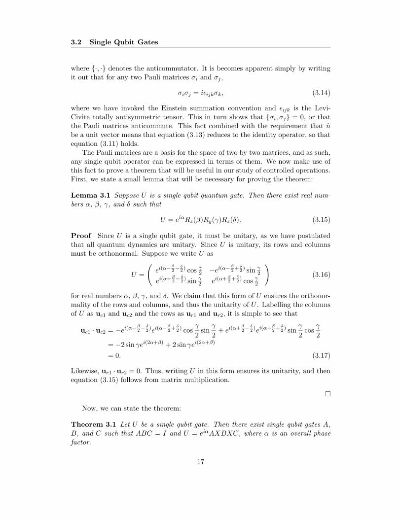
Lemma 3.1 Suppose U is a single qubit quantum gate. Then there exist real num-
bers α, β, γ, and δ such that
U = eiαRz(β)Ry(γ)Rz(δ). (3.15)
Proof Since U is a single qubit gate, it must be unitary, as we have postulatedthat all quantum dynamics are unitary. Since U is unitary, its rows and columnsmust be orthonormal. Suppose we write U as
U =
(
ei(α−β2− δ
2) cos γ2 −ei(α−β
2+ δ
2) sin γ
2
ei(α+ β2− δ
2) sin γ
2 ei(α+ β2+ δ
2) cos γ2
)
(3.16)
for real numbers α, β, γ, and δ. We claim that this form of U ensures the orthonor-mality of the rows and columns, and thus the unitarity of U . Labelling the columnsof U as uc1 and uc2 and the rows as ur1 and ur2, it is simple to see that
uc1 · uc2 = −ei(α−β2− δ
2)ei(α−
β2+ δ
2) cos
γ
2sin
γ
2+ ei(α+ β
2− δ
2)ei(α+ β
2+ δ
2) sin
γ
2cos
γ
2
= −2 sin γei(2α+β) + 2 sin γei(2α+β)
= 0. (3.17)
Likewise, ur1 · ur2 = 0. Thus, writing U in this form ensures its unitarity, and thenequation (3.15) follows from matrix multiplication.
�
Now, we can state the theorem:
Theorem 3.1 Let U be a single qubit gate. Then there exist single qubit gates A,
B, and C such that ABC = I and U = eiαAXBXC, where α is an overall phase
factor.
17

3.2 Single Qubit Gates
Proof Let us define
A ≡ Rz(β)Ry
(γ
2
)
B ≡ Ry
(
−γ2
)
Rz
(
−δ + β
2
)
C ≡ Rz
(δ − β
2
)
. (3.18)
Then we have
ABC = Rz(β)Ry
(γ
2
)
Ry
(
−γ2
)
Rz
(
−δ + β
2
)
Rz
(δ − β
2
)
= Rz(β)Rz(−β) = I. (3.19)
Now, note that, using equation (3.14),
XYX = iZX = i(iY ) = −Y. (3.20)
Therefore,
XRy(θ)X = X(cos θ + iY sin θ)X = cos θ − iY sin θ
= Ry(−θ), (3.21)
where we have used X2 = I. Similarly,
XRz(θ)X = Rz(−θ). (3.22)
With these identities in mind, we can show that
XBX = XRy
(
−γ2
)
Rz
(
−δ + β
2
)
= XRy
(
−γ2
)
XXRz
(
−δ + β
2
)
= Ry
(γ
2
)
Rz
(δ + β
2
)
. (3.23)
Thus,
AXBXC = Rz(β)Ry
(γ
2
)
Ry
(γ
2
)
Rz
(δ + β
2
)
Rz
(δ − β
2
)
= Rz(β)Ry(γ)Rz(δ), (3.24)
and thus, by lemma 3.1, we have
U = eiαAXBXC. (3.25)
18

3.2 Single Qubit Gates
�
Before leaving this section, we introduce three additional useful single qubitgates: the Hadamard gate H, phase gate S, and π/8 gate T . These three gates havematrix and projector representations given by
H =1√2
(1 11 −1
)
=1√2(|0〉 + |1〉) 〈0| +
1√2(|0〉 − |1〉) 〈1|
S =
(1 00 i
)
= |0〉 〈0| + i |1〉 〈1|
T =
(1 0
0 eiπ/4
)
= |0〉 〈0| + eiπ/4 |1〉 〈1| . (3.26)
Of these three gates, we shall use the Hadamard gate most frequently, and so let usinvestigate it further. Consider its projector representation, and notice that
H |0〉 =1√2(|0〉 + |1〉)
H |1〉 =1√2(|0〉 − |1〉). (3.27)
The Hadamard gate thus takes either of the computational basis states and puts itinto a superposition state. Consider now a tensor product of two Hadamard gatesacting on the two qubit state |00〉 = |0〉 ⊗|0〉 . Explicitly calculating this operation,we have
H⊗2 |0〉⊗2 =1√2(|0〉 + |1〉)⊗ 1√
2(|0〉 + |1〉) =
1
2(|00〉 + |01〉 + |10〉 + |11〉). (3.28)
Thus, we see that this combination of two Hadamard gates acting on the |00〉 stategives an even superposition of all the computational basis states for a two qubitsystem. Let us now generalize this result.
Look again at equation (3.27). It is clear that for an arbitrary single qubit state|φ〉 , we can write
H |φ〉 =1∑
k=0
(−1)φk |k〉√2
. (3.29)
Let us now generalize this to the case of n qubits. We have
H⊗n |φ1, φ2, . . . , φn〉 =∑
k1,...,kn
(−1)φ1k1+φ2k2+...+φnkn |k1, k2, . . . , kn〉√2n
, (3.30)
which we can summarize as
H⊗n |φ〉 =∑
k
(−1)φ·k |k〉√2n
. (3.31)
19

3.3 Controlled Operations
Here, φ · k represent the bitwise inner product of φ and k; that is, the sum modulo2 of the products of the individual digits of φ and k when both are written inbinary. Note also that we term such an n-fold tensor product of Hadamard gatesthe Hadamard transform. Let us now consider the case where |φ〉 = |0〉⊗n. In thatcase, φ · k = 0, and so
H⊗n |0〉⊗n =∑
k
|k〉√2n, (3.32)
which is again an even superposition of computational basis states. We will oftenmake use of this result.
3.3 Controlled Operations
Now that we have discussed single qubit dynamics and have determined how toconstruct any arbitrary single qubit gate using the Pauli matrices, let us move on tomultiqubit gates. The most important class of multiqubit gates, and as we shall seethe only class we need concern ourselves with, is the class of controlled operations.
A controlled operation is a single qubit operation performed on a target qubitpredicated on the values of one or more control qubits. The most important ofthe controlled operations, and indeed also the simplest, is the control-not gate.This gate flips the value of the target qubit if the control qubit is in the |1〉 state,and it is the quantum analog of the classical xor gate (see Appendix A). In thecomputational basis, the control-not gate is given by
CN =
1 0 0 00 1 0 00 0 0 10 0 1 0
= |00〉 〈00| + |01〉 〈01| + |10〉 〈11| + |11〉 〈10| , (3.33)
where we have abbreviated the two-qubit tensor product states by using two labelsin the kets. Figure 3 shows the representation of both the control-not gate as wellas a general controlled-U gate.
We now show how to construct a general controlled operation. Recall fromtheorem 3.1 that an arbitrary single qubit gate U can be written U = eiαAXBXC.The first step in our construction is to perform a controlled phase shift by α; thatis, we want to rotate the phase of the target qubit if the control qubit is in the state|1〉 . This two-qubit transformation is given by
CP = |00〉 〈00| + |01〉 〈01| + eiα |10〉 〈10| + eiα |11〉 〈11|
=
1 0 0 00 1 0 00 0 eiα 00 0 0 eiα
. (3.34)
20

3.3 Controlled Operations
U(a) (b)
Figure 3: (a) A control-not gate. The dark dot represents the controlqubit, while the open circle represents the target qubit. (b) A more generalcontrolled-U operation.
We note, however, that this transformation can be decomposed into two single qubitoperations, since
(1 00 eiα
)
⊗ I =
1 0 0 00 1 0 00 0 eiα 00 0 0 eiα
. (3.35)
Here, the leftmost operator in the tensor product acts only on the control qubit andthe rightmost only on the target qubit. Thus, since target qubit is acted upon bythe identity in this transformation, the controlled phase shift can be replaced with asingle qubit transformation on the control qubit. Now, consider the circuit in Figure4; we claim that this circuit implements a general controlled operation. To see why
A B C
(1 0
0 eiα
)
Figure 4: A circuit implementing an arbitrary controlled U operation,where U = eiαAXBXC.
21

3.4 Universal Gate Sets
this should be, first notice that a control-not is exactly a controlled X operation,which makes sense given that the X gate is the quantum analog of a classical not
gate, as is easy to show using the definition in equation (3.3):
X |0〉 = (|0〉 〈1| + |1〉 〈0|) |0〉 = |1〉X |1〉 = (|0〉 〈1| + |1〉 〈0|) |1〉 = |0〉 . (3.36)
We now have two cases to consider: first, suppose the control qubit is in thestate |0〉 . In this case, the two control-not gates do not change the state of thetarget qubit, and the transformation ABC is applied to the target qubit. But, aspart of theorem 3.1, ABC = I, and so if the control qubit is not set the state of thetarget qubit does not change. Now, suppose the control qubit is in the state |1〉 .In this case, the transformation eiαAXBXC is applied to the target qubit, which isexactly U . The circuit in Figure 4 does indeed then implement a general controlledU operation.
Finally, we introduce one more piece of notation before moving on. We havethus far only considered controlled operations that perform some transformation ifa control qubit is in the |1〉 state. We can just as easily perform the transformationif the control qubit is in the |0〉 state. We use an open circle to denote a controlof this type, as shown in Figure 5. We also note that since the X operator is
=X X
Figure 5: A controlled operation conditioned on the control qubit beingin the |0〉 state and its implementation using a control-not gate.
the analog of a classical not gate, we may use it to map this new kind of controloperation into the type we have already discussed.
3.4 Universal Gate Sets
Now that we have discussed single and double qubit gates, we are ready to move onto the subject of universal sets. A universal gate set is a finite set of logic gates thatcan be used to implement any arbitrary circuit. As an example, the nand gate, anand gate with its output inverted, is universal for classical computation. In thissection, we develop a quantum gate set that is universal for quantum computation.
22

3.4 Universal Gate Sets
Ours will be an approximate universal set, but it can approximate any unitarytransformation to arbitrary accuracy. Following Nielsen and Chuang[1], we firstprove the universality of two-level unitary matrices and successively refine this setuntil we have a discrete universal set.
3.4.1 Two-Level Unitary Matrices
Consider a quantum gate U that acts on n qubits. Letting d = 2n, this gate actson a d-dimensional Hilbert space, and so can be written in the computational basisas a d × d matrix. We define a two-level unitary operation to be one that actsnontrivially on only a single qubit. We claim that we can find two level unitarymatrices Ud−1 to U1 such that Ud−1Ud−2 . . . U2U1U = V1 is a matrix with a one asthe top left element and all zeros in the rest of the first row and column [6]. Werepeat this process so that
VkVk−1 . . . V1U = I, (3.37)
and soU = V †
1 V†2 . . . V
†k . (3.38)
Rather than prove this in general, we explicitly construct the 3 × 3 case. Eventhough quantum gates can never have an odd number of rows and columns, the3 × 3 case is simpler than the 4 × 4 case, and is the first nontrivial example ofthe decomposition process we are demonstrating. Thus, while our example is not arealistic one for quantum computation, it contains the same fundamental steps andis easier to follow.
Consider the matrix
U =
a d gb e hc f j
(3.39)
where the elements of U satisfy the unitarity condition and are in general complex.We claim that we can write U3U2U1U = I for two level unitary matrices U3, U2, andU1. Let us first consider U1. Our goal is to make the entry [U1U ]21 zero; if b = 0,then, we can simply set U1 = I. Otherwise, let us choose a two level unitary matrixof the following form:
U1 =
α β 0γ δ 00 0 1
. (3.40)
23

3.4 Universal Gate Sets
Forming the product U1U , we get
U1U =
α β 0γ δ 00 0 1
a d gb e hc f j
=
(αa+ βb) (αd+ βb) (αg + βh)(γa+ δb) (γd+ δe) (γg + δh)
c f j
=
a′ d′ g′
b′ e′ h′
c′ f ′ j′
. (3.41)
Now, we want b′ = γa+ δb = 0. Observe that we can accomplish this by setting
γ =b
√
|a|2 + |b|2
δ =−a
√
|a|2 + |b|2. (3.42)
Since U1 must also be unitary, these choices for γ and δ force
β =b∗
√
|a|2 + |b|2. (3.43)
For reasons that will become clear shortly, we also choose to set
α =a∗
√
|a|2 + |b|2. (3.44)
Next, we consider U2U1U . We would like the lower left corner entry of this matrixproduct to be zero. If it is already, we simply set
U2 =
a′∗ 0 00 1 00 0 1
. (3.45)
If not, we choose a two level unitary matrix of the form
U2 =
α′ 0 β′
0 1 0γ′ 0 δ′
. (3.46)
24

3.4 Universal Gate Sets
Multiplying the matrices out, we obtain, in much the same way as above,
α′ =a′∗
√
|a′|2 + |c′|2
β′ =c′∗
√
|a′|2 + |c′|2
γ′ =c′
√
|a′|2 + |c′|2
δ′ =−a′
√
|a′|2 + |c′|2(3.47)
Thus, we obtain
U2U1U =
1 d′′ g′′
0 e′′ h′′
0 f ′′ j′′
. (3.48)
Since all of U2, U1, and U are unitary, their product is as well. In order to fulfill theunitarity condition, d′′ = g′′ = 0, so that
U2U1U =
1 0 00 e′′ h′′
0 f ′′ j′′
. (3.49)
Note that our somewhat arbitrary choice of α and α′ above was contrived to giveus a one in the upper left hand corner of this product. Now, we need simply set
U3 =
1 0 00 e′′∗ h′′∗
0 f ′′∗ j′′∗
(3.50)
and we will obtain, as desired, U3U2U1U = I, so that U = U †1U
†2U
†3 . We have
therefore decomposed a general 3 × 3 unitary matrix into a product of two levelunitary matrices. In terms of the more general expressions in equations (3.37) and(3.38), we have found that V1 = U2U1 and V2 = U3. Recall that V1 is a matrixsuch that the product V1U has a one in the upper left entry and zeros in the restof the first row and column. Looking at equation (3.49), this is clearly the case.
With this choice of V2, we also have that U = V †1 V
†2 , as desired. This algorithm
clearly generalizes to higher dimensions. For example, in the 4× 4 case, the matrixV1U would again have a one in the upper left entry and zeros in the rest of the firstrow and column. Acting recursively, we would the find a matrix V2 such that thenon-trivial 3× 3 submatrix of V1U would take on the same structure in the productV2V1U , and so on until we have fully decomposed the original matrix.
25

3.4 Universal Gate Sets
3.4.2 Single Qubit and Control-NOT Gates
Now that we have shown that any arbitrary quantum gate can be implemented bytwo level unitary matrices, we continue on towards a discrete universal gate set byshowing that an arbitrary two level unitary operation can be implemented usingonly single qubit gates and the control-not gate.
Suppose U is a two level unitary operation. Let U be the nontrivial 2 × 2submatrix of U . We will prove that U can be implemented by single qubit gatesand the control-not gate by explicit construction. Let |s〉 and | t〉 be the twocomputational basis states one which U acts nontrivially . Let us define |g1〉 =|s〉 and |gm〉 = | t〉 . The states |g2〉 and |gm−1〉 are defined such that any twoconsecutive states |gi〉 and |gi+1〉 differ only by one bit; in other words, the states{|gi〉} form a Gray code from |s〉 to | t〉 . As an example of this, let us form a Graycode from |0110〉 to |1000〉 . We have
|g1〉 = |0110〉|g2〉 = |1110〉|g3〉 = |1100〉|g4〉 = |1000〉 (3.51)
The idea of our construction is this: begin with |g1〉 . By assumption, it differsfrom |g2〉 by a single bit. We thus swap these two states by using a controlled bitflip with its target being the bit where |g1〉 and |g2〉 differ. The bit flip will beconditioned by the requirement that all the other bits of |g1〉 and |g2〉 must be thesame. We iterate this process until we have transformed |gm−2〉 into |gm−1〉 . Atthis point, we performed a controlled U operation with its target being the qubitwhere |gm−1〉 and |gm〉 differ conditioned on all the other qubits being set. We thenproceed to undo all the swaps we have made.
As an example of this procedure, consider the three-qubit transformation
U =
1 0 0 0 0 0 0 00 1 0 0 0 0 0 00 0 a 0 0 0 0 b0 0 0 1 0 0 0 00 0 0 0 1 0 0 00 0 0 0 0 1 0 00 0 0 0 0 0 1 00 0 c 0 0 0 0 d
, (3.52)
where
U =
(a bc d
)
(3.53)
is an arbitrary unitary matrix. We note that U acts nontrivially on the basis states
26

3.4 Universal Gate Sets
|010〉 and |111〉 , on which it has the action
U |010〉 = a |010〉 + c |111〉U |111〉 = b |010〉 + d |111〉 . (3.54)
The Gray code states for this gate are given by
|g1〉 = |010〉|g2〉 = |011〉|g3〉 = |111〉 . (3.55)
Based on our procedure defined above, the circuit implementing U is shown inFigure 6. Consider the action of this circuit on a register in the state |010〉 , so
U
Figure 6: A circuit implementing the three-qubit gate U . Each of thethree controlled operations is conditioned on two control qubits.
that the top wire in Figure 6 carries a qubit in the |0〉 state, the middle wire a |1〉 ,and the bottom wire a |0〉 . The first operation is a control-not gate conditionedon the top qubit being a |0〉 and the middle qubit being a |1〉 . Since both the topand middle qubits do in fact have these values, we invert the state of the bottomqubit, leaving us in the state |011〉 .
The second gate in Figure 6 is a controlled U operation on the top qubit, condi-tioned on the both middle and bottom qubits being |1〉 . Since both are in the |1〉 ,state, the U operation is applied to the top qubit, so that after two operations weare in the state a |011〉 + c |111〉 .
Finally, the third operation is another control-not gate with the same condition-ing as before. Thus, we finally obtain the state a |010〉 + c |111〉 , which is exactlywhat we found before in equation (3.54).
A similar line of reasoning can be used to find the action of the circuit in Figure6 on the state |111〉 :
|111〉 → |111〉 → b |011〉 + d |111〉 → b |010〉 + d |111〉 . (3.56)
27

3.4 Universal Gate Sets
Likewise, it is straightforward to show that any other state passes through thiscircuit unchanged. Thus, the circuit in Figure 6 reproduces the operation of U .
We have now shown how to implement an arbitrary two level unitary gate usingonly controlled operations. Recall, though, that in Section 3.3, we showed that anarbitrary controlled operation may be implemented using only single qubit gatesand the control-not gate; thus, we have now proved these gates to be universal.
3.4.3 A Discrete Universal Set
We are now finally in a position to provide a discrete set of quantum gates that isuniversal for quantum computation. Our set will consist of the control-not gate,the Hadamard gate H, and the π/8 gate T . It is also common to include the phasegate in this set since its inclusion is natural when considering fault-tolerant gateconstructions; however, since the phase gate S is simply T 2, we do not include ithere.
Our set of gates will be an approximate universal set. Since the space of allunitary transformations is continuous, we obviously cannot truly construct it witha finite number of transformations. However, we will see that our universal set canapproximate any unitary transformation to arbitrary accuracy.
Consider the T gate and the combination HTH. From the definition of therotation operators in equation (3.10), it is clear that the T gate is, up to a phasefactor, a rotation by π/4 radians about the z axis. Similarly, HTH is a rotation byπ/4 radians about the x axis, up to a phase, as shown below:
HTH =1
2
(1 11 −1
)(1 0
0 eiπ/4
)(1 11 −1
)
=1
2
((1 + eiπ/4) (1 − eiπ/4)
(1 − eiπ/4) (1 + eiπ/4)
)
(3.57)
Since
1 + eiπ/4 = 1 + cosπ
4+ i sin
π
4= 2 cos2
π
8+ 2i sin
π
8cos
π
8
= 2eiπ/8 cosπ
8(3.58)
and
1 − eiπ/4 = 1 − cosπ
4− i sin
π
4= 2 sin2 π
8− 2i sin
π
8cos
π
8
= −2ieiπ/8 sinπ
8, (3.59)
we have
HTH = eiπ/8(
cos π8 −i sin π8
−i sin π8 cos π8
)
= Rx
(π
4
)
. (3.60)
28

3.4 Universal Gate Sets
Now, let us consider the composition of these two rotations:
e−iπZ/8e−iπX/8 =(
cosπ
8− iZ sin
π
8
)(
cosπ
8− iX sin
π
8
)
= cos2π
8− i[
(X + Z) cosπ
8+ Y sin
π
8
]
sinπ
8. (3.61)
Comparison with equation (3.11) shows that this is a rotation about the axis n =(cos π8 , sin
π8 , cos
π8 ) through an angle φ defined by cos φ2 = cos2 π
8 . Though we donot present the proof, this φ can be shown to be an irrational multiple of 2π [7].
We would like to be able to represent a rotation through any angle θ by repeatedapplication of Rn(φ). We note that since φ is an irrational multiple of 2π, φ = 2λπwhere λ is irrational. For any arbitrary θ, there is an integer k such that
eikπλ ≈ eiθ, (3.62)
since phase factors are defined modulo 2π. Thus, Rn(φ) can be used to approximatea rotation of any angle. Now, consider the product HRn(φ)H. Using the fact thatH = 1√
2(X + Z) and that H is Hermitian as well as unitary, we have
HRn(φ)H = cos2π
8− i[
(X + Z) cosπ
8+HYH sin
π
8
]
sinπ
8. (3.63)
Since
HYH =1
2(X + Z)Y (X + Z) =
1
2(X + Z)(−iZ + iX)
=1
2(−Y − Y ) = −Y, (3.64)
we haveHRn(φ)H = cos2
π
8− i[
(X + Z) cosπ
8− Y sin
π
8
]
sinπ
8, (3.65)
which is a rotation about the m = (cos π8 ,− sin π8 , cos
π8 ) axis, where m and n are not
parallel. Up to a phase shift, any single qubit gate can be represented as a product ofrotations about two nonparallel axes, and so any single qubit gate can be representedby an appropriate product of Rn(θ) and Rm(θ). Since we can approximate these twogeneral rotations using only the Hadamard and π/8 gates, we need only H and T toimplement any arbitrary single qubit gate. With the results of the previous sectionsin mind, then, we have constructed a universal set of gates. Any quantum circuitcan be approximated to arbitrary accuracy by the Hadamard, π/8, and control-not
gates.
29

4 Quantum Algorithms
4 Quantum Algorithms
4.1 Introduction
The power of quantum computation becomes most evident in the study of quantumalgorithms. Strictly speaking, a quantum computer is no more powerful than aclassical computer; there is no function computable by a quantum computer thatis not also computable by a classical computer. There are, however, tasks whicha quantum computer can perform significantly faster than a classical computer isthought to be able to, using what is known as quantum parallelism.
The idea behind quantum parallelism is simple. Since a register of n qubitscan be prepared in a superposition of all its basis states, and can therefore representsimultaneously all numbers between 0 and 2n−1, any unitary transformation actingon this register must transform every one of these basis states with a single operation.After a single application of the unitary transformation, the quantum register is leftin a superposition of all possible answers. This seems too good to be true, and inmany ways it is; a measurement of the register must, of course, yield only a singleresult, and in the process destroys the superposition. This collapse would seemto argue that nothing has been gained over a classical computation of the samefunction. The known quantum algorithms, however, cleverly take advantage of thefact that the amplitudes of the superposition of the result register may be adjustedusing quantum interference in order to produce their remarkable results.
The general pattern for quantum algorithms is thus clear: first, a quantumregister is prepared in an even superposition, in which every state has the samecoefficient, of its basis states. Next, some function is evaluated on this superpositionusing a unitary transformation. Finally, the register is interfered by means of aFourier or Hadamard transform, and is then measured to obtain a result.
In this section, we present the major known quantum algorithms. Deutsch’salgorithm and its extension, the Deutsch-Jozsa, algorithm have no known applica-tions but are useful as introductions to the more complicated quantum algorithms.Grover’s search algorithm speeds up the search of an unstructured database of Nelements by a factor of
√N over a classical search, and has many applications.
Finally, Shor’s factoring algorithm, an application of the more general quantumorder-finding algorithm, can determine the prime factors of a composite numbermuch faster than the best known classical algorithm, and has important ramifica-tions for cryptography.
4.2 Deutsch’s Algorithm
Deutsch’s problem, first proposed and solved in Deutsch’s seminal paper [3], was thefirst example of a problem that could be solved faster on a quantum computer thanon a classical computer. While it has no known applications, both Deutsch’s algo-rithm and the Deutsch-Jozsa algorithm are important from a historical standpoint,
30

4.2 Deutsch’s Algorithm
and as simple introductions to quantum algorithms. Here, we present a simplifiedversion of the algorithm presented in Cleve et al. [8] and Nielsen and Chuang [1].
Deutsch’s problem supposes the existence of a black box that evaluates somefunction f : {0, 1} 7→ {0, 1}. There are four such functions: two constant functions,
f(0) = f(1) = 0 and f(0) = f(1) = 1, (4.1)
and two so-called balanced functions,
f(0) = 0, f(1) = 1 and f(0) = 1, f(1) = 0. (4.2)
We would like to determine which of these two categories of functions a given blackbox falls into. Classically, the only way to tell would be to evaluate both f(0)and f(1); even though we are not asking for the values explicitly, both evaluationsare necessary to determine the global function property. A quantum computer,however, can determine this global property with only a single function evaluation,using Deutsch’s algorithm. A quantum network depiction of Deutsch’s algorithm isshown in Figure 7.
H
H
H|0〉
|1〉
Uf
x
y
x
y ⊕ f(x)
Figure 7: A quantum circuit to implement Deutsch’s algorithm.
As shown in the figure, we begin with a two-qubit register initialized to the state|01〉 . Each of these qubits is passed through a Hadamard gate, putting the registerinto the state
|ψ〉 =
( |0〉 + |1〉√2
)( |0〉 − |1〉√2
)
. (4.3)
Next, we must evaluate the function f . This evaluation is accomplished by meansof the Uf operator, which some have called an f -control-not gate. This two-qubitgate inverts the second of its input qubits only if the value of f evaluated on its firstinput qubit is 1; thus, it performs the transformation
|x〉 |y〉 Uf−−→ |x〉 |y ⊕ f(x)〉 , (4.4)
31

4.2 Deutsch’s Algorithm
where ⊕ denotes addition modulo 2.3 We also note that
Uf
[
|x〉( |0〉 − |1〉√
2
)]
=1√2|x〉 [|0 ⊕ f(x)〉 − |1 ⊕ f(x)〉 ]
=
|x〉(|0〉−|1〉√
2
)
, f(x) = 0
|x〉(|1〉−|0〉√
2
)
, f(x) = 1
= (−1)f(x) |x〉( |0〉 − |1〉√
2
)
. (4.5)
After passing through the Uf gate, then, the circuit is in the state
Uf |ψ〉 = (−1)f(x)
( |0〉 + |1〉√2
)( |0〉 − |1〉√2
)
=
(|0〉+|1〉√
2
)(|0〉−|1〉√
2
)
, f(0) = f(1) = 0(|0〉−|1〉√
2
)(|0〉−|1〉√
2
)
, f(0) = 0, f(1) = 1
−(|0〉+|1〉√
2
)(|0〉−|1〉√
2
)
, f(0) = f(1) = 1
−(|0〉−|1〉√
2
)(|0〉−|1〉√
2
)
, f(0) = 1, f(1) = 1
, (4.6)
which can be more concisely summarized as
Uf |ψ〉 =
±(|0〉+|1〉√
2
)(|0〉−|1〉√
2
)
, f(0) = f(1)
±(|0〉−|1〉√
2
)(|0〉−|1〉√
2
)
, f(0) 6= f(1). (4.7)
Now, the first qubit is passed through another Hadamard gate, which produces thestate
± |0〉(|0〉−|1〉√
2
)
, f(0) = f(1)
± |1〉(|0〉−|1〉√
2
)
, f(0) 6= f(1). (4.8)
Now, noting that
f(0) ⊕ f(1) =
{0, f(0) = f(1)1, f(0) 6= f(1)
, (4.9)
we can rewrite the final state of the circuit as
|ψout〉 = ± |f(0) ⊕ f(1)〉( |0〉 − |1〉√
2
)
. (4.10)
3Addition modulo 2 produces the following results:
|0 ⊕ 0〉 = |0〉 |0 ⊕ 1〉 = |1〉
|1 ⊕ 0〉 = |1〉 |1 ⊕ 1〉 = |0〉
32

4.3 The Deutsch-Jozsa Algorithm
Thus, a measurement of the first qubit will give the value of f(0)⊕f(1); if this valueis 0, f is constant, and otherwise is balanced. Thus, with only a single evaluation,we have determined a global property of f .
Deutsch’s algorithm, while giving a 50% speedup over the fastest classical al-gorithm for the same task, is not a particularly stunning result. It contains theseeds,however, from which the other known quantum algorithms grow. Deutsch’salgorithm first throws its quantum register into an even superposition and then pro-ceeds to evaluate a function and interfere the outcomes to obtain its final result. Wewill see this pattern again in each of the other algorithms presented in this section.Next, we present the n-qubit extension of Deutsch’s algorithm, which, while similarto Deutsch’s algorithm, has a more impressive result.
4.3 The Deutsch-Jozsa Algorithm
The Deutsch-Jozsa algorithm is the n-qubit generalization of Deutsch’s algorithm,first published in a paper by Deutsch and Jozsa in 1992 [9]. Again, we present herean improved version of the algorithm from Cleve et al. [8] and Nielsen and Chuang[1].
Suppose we have a function f , now defined such that f : {0, 1}n 7→ {0, 1} for evenn, that is guaranteed to be either constant or balanced4. Our goal is to determinewith certainty which category f falls into. Classically, this would require, in theworst case, 2n−1 + 1 evaluations of f , since we could get 2n−1 0’s before finallygetting a 1. Quantum mechanically, however, this global property of f can onceagain be determined with only a single evaluation of f .
The algorithm proceeds much as Deutsch’s algorithm did; a quantum circuitdiagram for the algorithm is shown in Figure 8. As before, the input state of|0〉⊗n |1〉 is first sent through a Hadamard transform. As we have shown before inequation (3.32), a Hadamard transform on a quantum register in the |0〉⊗n stateproduces an even superposition of all the basis states of the register, so after theapplication of the Hadamard transform we have the state
|ψ〉 =
2n−1∑
x=0
|x〉√2n
( |0〉 − |1〉√2
)
, (4.11)
where we have acted with the Hadamard transform on the |1〉 qubit as well. Now,once again, we use the Uf operator to evaluate the function f , which gives
Uf |ψ〉 =2n−1∑
x=0
(−1)f(x) |x〉√2n
( |0〉 − |1〉√2
)
, (4.12)
4A constant n-qubit function is one that gives the same result for any input, and a balanced
n-qubit function is one that returns one result for exactly half of its inputs and a second result for
the other half of its inputs.
33

4.3 The Deutsch-Jozsa Algorithm
nH⊗n
H
H⊗n|0〉
|1〉
Uf
x
y
x
y ⊕ f(x)
Figure 8: A quantum circuit to implement the Deutsch-Jozsa algorithm.The wire with a / represents an n-qubit bus and is a shorthand notationfor n wires.
as we showed before. The result of the evaluation of f on every argument from 0to 2n − 1 is now stored in the first register. A direct measurement of this registerwould, of course, produce only a single result. However, by interfering the qubits,we may determine the global property of f we desire. To that end, we perform asecond Hadamard transform on the first register. Recall from equation (3.31) thatthe Hadamard transform on some register |φ〉 in general produces the state
H⊗n |φ〉 =∑
k
(−1)φ·k |k〉√2n
. (4.13)
Using this, we can write the state of our circuit after the second Hadamard transformas
∑
k
∑
x
(−1)x·k⊕f(x) |k〉2n
( |0〉 − |1〉√2
)
. (4.14)
Now, we measure the first register. It turns out that if k = 0, we know with certaintythat f is constant; if k 6= 0, then f is balanced. To see why this is true, considerequation (4.12). If f is constant for all values of its argument, this equation can berewritten as
Uf |ψ〉 = ±H⊗n |0〉⊗n( |0〉 − |1〉√
2
)
. (4.15)
Since the Hadamard transform is Hermitian as well as unitary (it being both sym-metric and real), the second Hadamard transform on this state produces
|0〉⊗n( |0〉 − |1〉√
2
)
. (4.16)
Thus, when every qubit in the first register is 0, f is constant. If f is balanced, wecannot make the simplification in equation (4.15), and at least one qubit in the firstregister will be nonzero.
34

4.4 Grover’s Algorithm
Amazingly, then, we have achieved an exponential speedup over the best classicalalgorithm for solving this problem, reducing the worst case number of functionevaluations from 2n−1 + 1 to a single evaluation.
4.4 Grover’s Algorithm
Now that we have seen some examples of simple quantum algorithms, we move onto an algorithm with practical application. Suppose we have an n qubit database ofunsorted data, and we wish to find elements that match a certain criterion. Sincewe are assuming that there is no structure to this database, the best we can doclassically is simply to search through the entire database until we come across theelement we seek. For an N = 2n element database, this will require O(N) queriesto the database. However, the quantum algorithm due to Grover can speed up thesearch for this “needle in a haystack” [10], allowing us to find the desired element inonly O(
√N) steps. We begin by presenting the algorithm itself, and follow with a
discussion of why the algorithm works. Finally, we present an alternate generalizedform of the algorithm.
4.4.1 Procedure
As with the Deutsch-Jozsa algorithm, Grover’s algorithm begins by applying aHadamard transform to the |0〉⊗n state, giving us the familiar even superposition
H⊗n |0〉⊗n =1√2n
2n−1∑
x=0
|x〉 . (4.17)
We next apply several instances of the so-called Grover operator G.The first part of the Grover operator is a black box known as an oracle that can
recognize the desired elements of our database.5This oracle O marks such states bygiving them local phase shifts of π radians; the internal workings of the oracle arenot specified by the algorithm. We can write the action of the oracle as
O |x〉 = (−1)δxτ |x〉 , (4.18)
where |τ〉 represents a solution of the search problem. We also note that
O = I − 2 |τ〉 〈τ | (4.19)
5It may seem as if the existence of an oracle that knows that answer to the search problem
obviates the need for the rest of the search algorithm. There are instances, however, where it is
possible to recognize the solution of a search problem without knowing the solution, especially when
using quantum parallelism. Consider what happens when the oracle operates on a quantum register
and one of the states in the register is the target state of search problem. The oracle will mark this
state, but without the rest of the search algorithm, there is no way to tell which state has been
marked since all the basis states of the register are entangled. In this case, even though the oracle
can recognize the solution, it cannot be used to find the solution by itself.
35

4.4 Grover’s Algorithm
since
(I − 2 |τ〉 〈τ |) |x〉 = |x〉 − 2 |τ〉 〈τ |x〉 = |x〉 − 2δxτ |τ〉
=
{|τ〉 − 2 |τ〉 = − |τ〉 , x = τ|τ〉 , x 6= τ
= (−1)δxτ |x〉 . (4.20)
The next part of the Grover operator is a Hadamard transform H⊗n. We then giveevery element of the database except for the |0〉 element a π phase shift. Just aswe can write the action of the oracle as in equation (4.19), we can write this step asan application of the operator
2 |0〉 〈0| − I, (4.21)
where the signs of the two halves of the operator are reversed since we are shiftingthe phase of every element except the 0th element; that is, we are performing thetransformation |x〉 → −(−1)δx0 |x〉 . Finally, the Grover operator contains a secondHadamard transform. The full Grover operator thus can be written
G = H⊗n(2 |0〉 〈0| − I)H⊗nO. (4.22)
In the next section, we discuss exactly what the operator does; we also calculatehow many times it must be applied.
After applying the Grover operator, all we must do to complete the algorithmis measure the register; with an arbitrarily high probability, the measured state willbe one of the desired target states.
4.4.2 Inversion about the Mean
The question remains as to what the Grover iteration actually does, and why it per-forms a database search. Consider that the essential operation of Grover’s algorithmis to take some initial state |γ〉 and transform it into some target state |τ〉 . For thealgorithm to work, then, repeated applications of the Grover operator must changethe one vector into the other. Let us define a two dimensional space spanned byvectors |α〉 and |β〉 where |β〉 is an even superposition of the solutions to our searchproblem and |α〉 is an even superposition of the nonsolutions; let us furthermoresuppose that there are N states in our database and M solutions. Normalizing thesetwo vectors, we have
|α〉 =1√
N −M
∑
nonsolutions
|x〉 (4.23)
and
|β〉 =1√M
∑
solutions
|x〉 . (4.24)
36

4.4 Grover’s Algorithm
We can reexpress the initial even superposition in terms of these new vectors (forconvenience, we make the definition |ψ〉 = 1√
N
∑
x |x〉). Since
|ψ〉 =1√N
(∑
nonsolutions
|x〉 +∑
solutions
|x〉)
, (4.25)
we have
|ψ〉 =1√N
(√N −M |α〉 +
√M |β〉
)
=
√
N −M
N|α〉 +
√
M
N|β〉 . (4.26)
Now we can see what the Grover operator does to the vector |ψ〉 in this space.The first part of the Grover operator is an application of the oracle. Recall that theoracle gives a π phase shift to all solutions of the search problem; thus, by definition,
O |ψ〉 = O
(√
N −M
N|α〉 +
√
M
N|β〉)
=
√
N −M
N|α〉 −
√
M
N|β〉 . (4.27)
This amounts to a reflection of |ψ〉 about the |α〉 -axis. The other part of theGrover operator, H⊗n(2 |0〉 〈0| − I)H⊗n, can be rewritten in our current notationas 2 |ψ〉 〈ψ| −I. Comparing this form to the form of the oracle in equation (4.19), wecan see that this second part of the Grover operator is also a reflection in the planedefined by |α〉 and |β〉 , this time about the original vector |ψ〉 . This operationis often called inversion about the mean; consider its action on a general state∑
k αk |k〉 :
(2 |ψ〉 〈ψ| − I)
(∑
k
αk |k〉)
=∑
k
[2αk |ψ〉 〈ψ| k〉 − αk |k〉 ]
=∑
k
2αkN
∑
i
∑
j
| i〉 〈j| k〉 − αk |k〉
=∑
k
2αkN
∑
i
∑
j
δjk | i〉 − αk |k〉
=∑
k
[
2αkN
∑
i
| i〉]
−∑
k
[αk |k〉 ] . (4.28)
We now swap the summations and define the average value of α to be 〈α〉 ≡∑
k αk/N to obtain
∑
i
[∑
k
2αkN
]
| i〉 −∑
k
αk |k〉 =∑
i
2〈α〉 | i〉 −∑
k
αk |k〉 . (4.29)
37

4.4 Grover’s Algorithm
Finally, we relabel the dummy index i by k, obtaining a final state of
∑
k
[−αk + 2〈α〉] |k〉 . (4.30)
The two halves of the Grover operator thus each perform a reflection in the sameplane, and since the product of two reflections is a rotation, the Grover operatoreffectively rotates the starting state towards the vector of solutions, as is shown inFigure 9. Continued applications of the Grover operator rotate the state closer and
|α〉
|β〉
|ψ〉
O |ψ〉
G |ψ〉
θ/2
θ/2
θ
Figure 9: The action of a single application of the Grover operator on thestate |ψ〉 .
closer to the solution vector, while remaining in the same space. So how many timesmust we apply the Grover operator to have a good chance of finding a solution?
Let us make the definition that
cosθ
2≡√
N −M
N. (4.31)
This defines the triangle in Figure 10, such that
sinθ
2=
√
M
N. (4.32)
We can therefore reexpress |ψ〉 as
|ψ〉 = cosθ
2|α〉 + sin
θ
2|β〉 . (4.33)
38

4.4 Grover’s Algorithm
θ/2√N −M
√M
√N
Figure 10: The triangle defined by equation (4.31).
Now, as can be seen from Figure 9, the Grover operator rotates |ψ〉 by exactly θradians; the oracle’s reflection effectively rotates the state by −θ radians and thesubsequent reflection about |ψ〉 rotates the state by 2θ radians.
We can now quantify the number of times we must apply the Grover operatorto our system to rotate |ψ〉 close to |β〉 . Consider again equation (4.26); our goalis to rotate this state close to the vector |β〉 . We now show that rotating throughan angle φ = Cos-1
√
M/N will take |ψ〉 to |β〉 .First, we note that φ is the complement of θ/2. Thus, we can easily write down
a rotation operator in the {|α〉 , |β〉} basis. We have
UR =
(cosφ − sinφsinφ cosφ
)
=
√MN −
√N−MN√
N−MN
√MN
. (4.34)
We now operate on |ψ〉 , which in this basis is
|ψ〉 =
√N−MN√MN
(4.35)
to obtain
UR |ψ〉 =
( √MN
√N−MN −
√MN
√N−MN(
N−MN
)+ M
N
)
=
(01
)
= |β〉 , (4.36)
as claimed.Since every application of the Grover operator rotates |ψ〉 through θ radians,
we must apply it
R =Cos-1
√MN
θ(4.37)
times to rotate |ψ〉 to |β〉 . In actuality, we require R to be an integer, and so Ris actually the integer closest to the value in equation (4.37). We now simplify this
39

4.4 Grover’s Algorithm
rather unwieldy expression by noting that, since the maximum value of Cos-1 is π/2,the upper bound on R is
R ≤⌈ π
2θ
⌉
. (4.38)
For M ≤ N/2 (we will explain this restriction shortly), we have, using equation(4.32),
θ
2≥ sin
θ
2=
√
M
N(4.39)
so that θ ≥ 2√
M/N and
R ≤⌈
π
4
√
N
M
⌉
. (4.40)
Thus, as stated earlier, Grover’s algorithm will run in O(√N) time.
Now, to see why the above expression was limited to the case of M ≤ N/2, wederive an expression for sin θ. First, let us apply a half-angle identity to equation(4.32), giving us
sinθ
2=
√
1 − cos θ
2=
√
M
N. (4.41)
Simplifying, this equation describes a triangle such that
cos θ =N − 2M
N. (4.42)
Using this triangle, we have
sin θ =2√
M(N −M)
N. (4.43)
Examining this expression, we can see that asM increases fromN/2 toN , θ becomessmaller, and thus R increases. Thus we have the strange behavior that Grover’salgorithm performs worse for databases where more than half of the elements aresolutions. Odd as this behavior is, we may escape from it simply by adding anotherN nonsolutions to our database. In this case, there will definitely be more than twiceas many nonsolutions as solutions, and Grover’s algorithm will perform optimally,with the same complexity as derived above.
4.4.3 An Alternate Approach
The above discussion of Grover’s algorithm seems intimately connected with theproperties of the Hadamard transform, as it appears twice in the Grover operatorwhich is the heart of the algorithm. Grover, however, also published a second, moregeneral version of his algorithm that shows that almost any unitary operator maybe used to search a quantum database [11].
40

4.4 Grover’s Algorithm
Recall that the goal of Grover’s algorithm is to take some initial state |γ〉 to atarget state |τ〉 . We have shown how the Grover operator G is able to perform thisoperation, using the Hadamard transform. Now consider an operator Q, defined as
Q = −IγU †IτU, (4.44)
whereIφ = I − 2 |φ〉 〈φ| (4.45)
and U is some arbitrary unitary transformation. We now operate with Q on |γ〉 :
Q |γ〉 = −IγU †IτU |γ〉= (2 |γ〉 〈γ| − I)U † (I − 2 |τ〉 〈τ |)U |γ〉=[
2 |γ〉 〈γ| − 4 |γ〉 〈γ| U † |τ〉 〈τ | U − I + 2U † |τ〉 〈τ | U]
|γ〉 . (4.46)
DefiningUτγ = 〈τ |U | γ〉 , (4.47)
we haveQ |γ〉 =
(
1 − 4 |Uτγ |2)
|γ〉 + 2Uτγ
(
U † |τ〉)
. (4.48)
This result suggests that we examine Q in the{|γ〉 , U † |τ〉
}basis. To that end, let
us calculate Q(U † |τ〉
):
Q(
U † |τ〉)
=(
−IγU †IτU)(
U † |τ〉)
= (2 |γ〉 〈γ|)U † (I − 2 |τ〉 〈τ |)UU † |τ〉=[
2 |γ〉 〈γ| U † − 4 |γ〉 〈γ| U † |τ〉 〈τ | − U † + 2U † |τ〉 〈τ |]
|τ〉
=(
U † |τ〉)
− 2U∗τγ |γ〉 . (4.49)
Thus, we see that Q preserves the space spanned by{|ψ〉 , U † |τ〉
}, and we can
write it in this basis as
Q
(|γ〉
U † |τ〉
)
=
(1 − 4 |Uτγ |2 2Uτγ
−2U∗τγ 1
)(|γ〉
U † |τ〉
)
. (4.50)
Now, we know that |Uτγ |2, being a normalized probability, is less than one. Assum-ing that both it and its associated amplitudes Uτγ and U∗
τγ are small, we can view
Q as a rotation of roughly 2 |Uτγ | in this space, from |γ〉 to U † |τ〉 . Thus, usingsimilar logic as above, Q can also search a database, using any convenient unitarytransformation.
So how many times must we apply Q to attain a high probability of finding asolution? In any situation of interest, we know that |γ〉 and U † |τ〉 are close toorthogonal. If they were not, then the bracket 〈τ |U | γ〉 would not be small, and
41

4.4 Grover’s Algorithm
so there would be a nonnegligible probability that an observation of U |γ〉 wouldproduce |τ〉 . If this were the case, then by simply conducting several repeatedexperiments, |τ〉 could be readily determined. Thus, the angle between |γ〉 andU † |τ〉 must be roughly π/2. Since every application of Q rotates the state byroughly 2 |Uτγ |, we must apply Q
r =(π
2
)( 1
2 |Uτγ |
)
=π
4 |Uτγ |
= O(
1
|Uτγ |
)
(4.51)
times. Thus, we have that|τ〉 ≈ UQ⊗r |γ〉 . (4.52)
Finally, let us recreate the original Grover operator G from Q. Recall that
G = H⊗n (2 |0〉 〈0| − I)H⊗n (I − 2 |τ〉 〈τ |) , (4.53)
which in our present notation is
G = U(−I0)U †Iτ , (4.54)
using H⊗n = U = U †. Now, we note that
U †GU = U †U(−I0)U †IτU
= −I0U †IτU
= Q. (4.55)
Thus, the Grover operator G may be written as simply a unitary transformation ofthe generalized Grover operator Q. We may also recover the complexity of Grover’salgorithm, as follows. We have shown that the generalized version of Grover’s al-gorithm is of order O(1/|Uτγ |). Thus, to recover the standard Grover’s algorithmcomplexity of O(
√N). We want
⟨τ∣∣H⊗n∣∣ 0
⟩=
1√N. (4.56)
This is simple to show. First, we have
⟨τ∣∣H⊗n∣∣ 0
⟩= 〈τ |
(
1√N
N−1∑
i=0
| i〉)
. (4.57)
Since |τ〉 is orthonormal to exactly one of the kets in the sum (assuming a singlesolution to the search problem), this bracket collapses simply to 1/
√N , and we
recover the complexity of the original Grover’s algorithm.
42

4.5 Shor’s Algorithm
4.5 Shor’s Algorithm
Even though the field of quantum computation was born in 1985 with Deutsch’sseminal paper [3], it was not until 1994, when Shor first published fast quantumalgorithms for factoring and finding discrete logarithms, that quantum computa-tion became a major field of research. Classically, factoring is a difficult prob-lem; while it has not been proved to be an exponential time problem, the bestknown classical algorithm, known as the Number Field Sieve, runs in a time ofO(exp((logN)
13 (log logN)
23 )) for a number N [12]. Amazingly, Shor’s algorithm
can factor a number in only O((logN)2(log logN)(log log logN)) steps [13]. Thevast difference between these two time complexities can be seen in Figure 11, inwhich each of these functions is plotted against the logarithm base 2 of N , whichgives the number of bits in N when N is represented in binary.
The intense interest generated by the publishing of Shor’s factoring algorithmsprang not only from the fact that his algorithm was exponentially faster than thebest known classical algorithm, an impressive result in and of itself, but also from amore practical perspective. Since factoring has long been assumed to be a difficultproblem for large numbers, it was used as the basis for the RSA cryptosystem,one of the most widespread cryptosystems in use today. Thus, a working quantumcomputer running Shor’s algorithm could quickly and efficiently gain access to hugeamounts of encrypted data. Needless to say, this prospect generated widespreadinterest.
4.5.1 Number Theoretic Background
Shor’s algorithm relies on a trick from number theory for its efficiency. It is wellknown that the problem of factoring a composite number may be mapped into theequivalent problem of finding the order of a periodic function. Following Nielsenand Chuang [1] and Ekert and Jozsa [14], we now present this reduction.
Suppose N is a positive integer and x is some integer relatively prime to N suchthat 1 ≤ x < N . We define the order of f(x) = x mod N to be the least r suchthat xr ≡ 1 mod N . Finding such an r given x and N is referred to as the order-finding problem, for which there is no known efficient classical algorithm. It is thisorder-finding problem for which Shor determined an efficient quantum algorithm.
The heart of the reduction of factoring to order finding is the following theorem:
Theorem 4.1 Let N be a composite number and let x be a nontrivial solution to
x2 ≡ 1 mod N (4.58)
in the range 1 ≤ x < N , with gcd(x,N) = 1. We define a trivial solution to
be x ≡ ±1 mod N . Then, at least one of gcd(x + 1, N) or gcd(x − 1, N) is a
nontrivial factor of N .
43
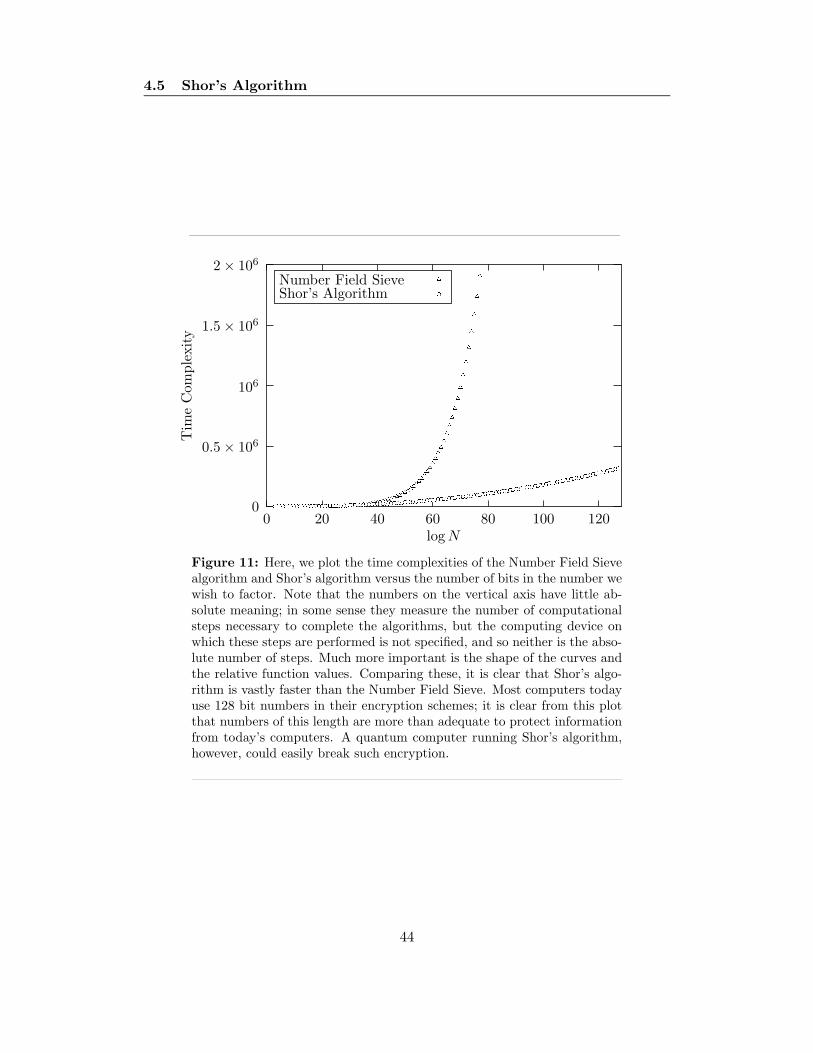
4.5 Shor’s Algorithm
0
0.5 × 10⁶
106
1.5 × 10⁶
2 × 10⁶
0 20 40 60 80 100 120
Tim
eC
omple
xity
logN
Number Field Sieve
�� �� �� �� � � � �� �� �� �� �� �� �� �� �� ! "# $% &' () *+ ,- ./ 01 23 45 67 89 :; <= >? @A BC DE FG HI JK LMNO PQ RS TU VW XY
Z[ \] ^_ `abc de fg
hi jklm no
pq rstu
vwxy
z{|}
~���
����
��
��
��
��
��
��
��
����
Shor’s Algorithm
�� �� �� �� ¡ ¢£ ¤¥ ¦§ ¨© ª« ¬ ®¯ °± ²³ ´µ ¶· ¸¹ º» ¼½ ¾¿ ÀÁ Âà ÄÅ ÆÇ ÈÉ ÊË ÌÍ ÎÏ ÐÑ ÒÓ ÔÕ Ö× ØÙ ÚÛ ÜÝ Þß àá âã äå æç èé êë ìí îï ðñ òó ôõ ö÷ øù úû üý þÿ�� �� �� �� � � � �� �� �� �� �� �� �� �� �� ! "#
$% &' () *+ ,- ./ 01 23 45 67 89 :; <= >?@A BC DE FG HI JK LM NO PQ RS TU
VW XY Z[ \] ^_ `a bc de fg hijk lm no pq rs tu vw xyz{ |} ~� �� �� �� �� �� ��
�� �� �� �� �� �� �� ���� �� ¡ ¢£ ¤¥ ¦§ ¨©
ª«
Figure 11: Here, we plot the time complexities of the Number Field Sievealgorithm and Shor’s algorithm versus the number of bits in the number wewish to factor. Note that the numbers on the vertical axis have little ab-solute meaning; in some sense they measure the number of computationalsteps necessary to complete the algorithms, but the computing device onwhich these steps are performed is not specified, and so neither is the abso-lute number of steps. Much more important is the shape of the curves andthe relative function values. Comparing these, it is clear that Shor’s algo-rithm is vastly faster than the Number Field Sieve. Most computers todayuse 128 bit numbers in their encryption schemes; it is clear from this plotthat numbers of this length are more than adequate to protect informationfrom today’s computers. A quantum computer running Shor’s algorithm,however, could easily break such encryption.
44

4.5 Shor’s Algorithm
Proof Let us begin by rewriting x2 ≡ 1 mod N as x2 − 1 ≡ 0 mod N . It is thenclear that N must divide x2 − 1 = (x + 1)(x − 1). Thus, N must have a commonfactor with either (x + 1) or (x − 1). Recognizing that −1 mod N = N − 1, thecondition that x is not a trivial solution becomes
1 < x < N − 1, (4.59)
which in turn leads tox− 1 < x+ 1 < N, (4.60)
and so the common factor cannot be N itself. Thus, either gcd(x+1, N) or gcd(x−1, N) must be a factor of N .
�
Now let x ≡ yr/2 mod N where r is the order of y mod N . Squaring thisexpression, we have
x2 ≡ yr ≡ 1 mod N, (4.61)
where the second equality follows from the definition of the order. It is then clearthat one of gcd(yr/2 +1, N) or gcd(yr/2 −1, N) is a nontrivial factor of N . Thus, byfinding the order modulo N of a number relatively prime to N , we can find a factorof N . Since there exists a fast classical algorithm to find greatest commons divisors(see Appendix B), an efficient algorithm for order finding can easily be mappedinto an efficient algorithm for factoring. In the following section, we present Shor’squantum order finding algorithm.
4.5.2 Order Finding
As shown above, the factoring problem is easily reduced to the problem of findingthe order of a periodic function. The heart of Shor’s factoring algorithm is thusan efficient order finding algorithm that depends crucially on the properties of thequantum Fourier transform, as we will now show.
Let us define a unitary transformation Uf such that
Uf |x〉 |0〉 = |x〉 |f(x)〉 , (4.62)
wheref(x) = yx mod N, (4.63)
where y is chosen such that gcd(y,N) = 1 so that y and N are relatively prime. Thismodular exponentiation operator can be implemented efficiently;for our purposes,however, we treat it simply as a black box. Now, let us begin the order findingalgorithm by initializing two quantum registers to |0〉⊗q, where q is a power of twosatisfying N2 ≤ q ≤ 2N2:
|ψ0〉 = |0〉⊗ log q |0〉⊗ log q . (4.64)
45

4.5 Shor’s Algorithm
This choice of q ensures that the quantum Fourier transform we use momentarilymay be computed efficiently. Note that |ψ0〉 is a tensor product of log q qubitsbecause we are here representing numbers in binary, and log q is the number ofbits in the number q. We then apply a Hadamard transform to the first register,obtaining
H⊗ log q |ψ0〉 =1√q
q−1∑
x=0
|x〉 |0〉⊗ log q = |ψ1〉 . (4.65)
Now, we apply the Uf operator defined above to this state:
Uf |ψ1〉 =1√q
q−1∑
x=0
|x〉 |f(x)〉 . (4.66)
Now, we measure the second register, obtaining some value y0. Because the tworegisters were entangled by the Uf operator, this measurement projects the firstregister into a superposition of all x such that f(x) = y0. Let us define x0 to bethe smallest such x. We know that y0 = yx0 mod N . Letting r be the order of fmodulo N , we also know that y0 = yx0+kr mod N for k ∈ [0,K] where K is definedas
K =
⌈q − x0
r
⌉
. (4.67)
Incorporating these ideas, the state of the system after the measurement is
|φ〉 =1√K
K−1∑
k=0
|x0 + kr〉 |y0〉 . (4.68)
At this point, the second register has served its purpose, and we drop it from ourdiscussion. Now, let us apply an q dimensional quantum Fourier transform to thefirst register, where the Fourier transform operator is
Fq =1√q
q−1∑
b,c=0
|c〉 e2πibc
q 〈b| . (4.69)
This gives us the state
Fq |φ〉 =1√qK
K−1∑
k=0
q−1∑
b,c=0
|c〉 e2πibc
q 〈b |x0 + kr 〉
=
q−1∑
c=0
[
1√qK
K−1∑
k=0
e2πi(x0+kr)c
q
]
|c〉
=
q−1∑
c=0
[
1√qK
(K−1∑
k=0
e2πikrc
q
)
e2πix0c
q
]
|c〉 . (4.70)
46

4.5 Shor’s Algorithm
Using the orthonormality condition for complex Fourier series,
Q−1∑
q=0
e2πiaq
Q e2πibq
Q = Qδab, (4.71)
and the fact that K ≈ q/r, the term in parentheses in equation (4.70) reduces to[14]
q
rδc,0 mod (q/r), (4.72)
which says that c must be a multiple of q/r. Let c = j qr . Then we have
Fq |φ〉 =1√r
r−1∑
j=0
e2πijx0
r
∣∣∣jq
r
⟩
. (4.73)
A measurement of this register will now give us some c such that
c
q=λ
r(4.74)
where c and q are known. By using a continued fractions expansion (see AppendixB), we can now determine the period r.
In our discussion of the order finding algorithm above, we have assumed (equa-tion (4.72)) that the Fourier transform generates constructive interference only forthose c that are multiples of q/r. This, however, is not strictly the case. In fact, forthe algorithm to produce the order of f(x) with high probability, c need only meetthe condition [13]
−r2≤ rc mod q ≤ r
2, (4.75)
which is equivalent to
|rc− dq| ≤ r
2(4.76)
for some d. Rearranging this expression, we have
∣∣∣∣
c
q− d
r
∣∣∣∣≤ 1
2q. (4.77)
Again, since c and q are known, we may find the period r by again using a continuedfractions expansion. As long as this period is even, we know that at least one ofgcd(yr/2 + 1, N) or gcd(yr/2 − 1, N) is a nontrivial factor of N . If r is odd, thealgorithm fails, and we must try again with a different choice of y.
47

4.5 Shor’s Algorithm
4.5.3 An Example: Factoring 15
Here, we illustrate Shor’s algorithm with a relatively simple example. We choose tofactor N = 15, as this is the smallest composite number that is neither even nor thesquare of a prime. Thus, N = 15 is the first nontrivial number to factor.
First, we need to pick some y relatively prime to 15; let y = 7. We also needa q that is a power of two and satisfies 152 ≤ q ≤ 2(152); let q = 256. Using thenotation above, we begin with the state
|ψ0〉 = |0〉⊗8 |0〉⊗8 . (4.78)
The first step of the algorithm is to apply the Hadamard transform to the firstregister, giving us
H⊗8 |ψ0〉 =1√256
255∑
x=0
|x〉 |0〉⊗8 = |ψ1〉 . (4.79)
We next apply the Uf operator to the second register, giving us
Uf |ψ1〉 =1√256
255∑
x=0
|x〉 |7x mod 15〉
=1√256
[|0〉 |1〉 + |1〉 |7〉 + |2〉 |4〉 + |3〉 |13〉 + |4〉 |1〉 + . . .] . (4.80)
It is clear from this expression that r = 4. Despite this, we continue with thealgorithm, since in general the order finding problem will not be as simple. Thenext step is the measure the second register to obtain some y0; suppose we findy0 = 13. The first register will then be in a superposition of all the x values thatgive f(x) = 13. We can see from equation (4.80) that x0, the smallest of these xvalues, is 3. Dropping the second register, just as we did above, the state of the firstregister after the measurement is given by
|φ〉 =1√64
[|3〉 + |7〉 + |11〉 + |15〉 + . . .] . (4.81)
Now, we must take the Fourier transform of |φ〉 . Using equation (4.73), we have
F256 |φ〉 =1√r
r−1∑
j=0
e6πij
r
∣∣∣∣j256
r
⟩
. (4.82)
A measurement of the register now will give either 0, 64, 128, or 192, each with thesame probability. Now, using equation (4.74), quickly see that, indeed, r = 4. Now,since r is even, we know that at least one of
gcd(72 + 1, 15) = gcd(50, 15) = 5 (4.83)
48

4.5 Shor’s Algorithm
orgcd(72 − 1, 15) = gcd(48, 15) = 3 (4.84)
is a nontrivial factor of 15. In fact, each of these is a nontrivial factor; thus, we havesuccessfully used Shor’s algorithm to factor 15.
49

5 Linear Optics Quantum Computation
5 Linear Optics Quantum Computation
5.1 Why Linear Optics?
Of the proposed physical realizations of quantum computation, none is simpler thanlinear optics quantum computation (LOQC) [15]. While not a feasibly scalableimplementation, there are many advantages to LOQC. First and foremost, the sub-ject of quantum optics is well understood both theoretically and experimentally. Awide range of experimental techniques allowing the manipulation of single photons,which in LOQC are used as qubits, are known. Indeed, single photons provide sev-eral choices for the definition of qubits. Quantum information can be encoded in aphoton’s two orthogonal polarization states, in different spatial modes of a photon,or in some combination of the two [16]. In this section, we focus more on usingphoton spatial modes as our qubits, since, in theory, a single photon may then beused to represent an entire quantum register when sent through a multiport beamsplitter, as shown below.
There are also, unfortunately, some major disadvantages to LOQC. The pri-mary issue, and the one that prevents LOQC from being a fully realizable solutionfor quantum computation, is that the number of optical devices necessary to buildquantum circuits tends to scale exponentially with the number of qubits. Also, whenusing free space optics, component alignment can be very challenging. Since a linearoptics quantum computer is at its heart a complex interferometer, all the issues ininterferometer design and construction carry over to any experimental implemen-tation of LOQC. Finally, some multi-qubit gates are much simpler to implementexperimentally using nonlinear optical effects; for the most part, though, we avoidsuch constructions due to the additional (and somewhat unnecessary) theoreticalcomplexity.
Even though LOQC is not scalable, it can be used to implement small quantumcircuits relatively simply, and serves as an excellent test bed for proof of principleexperiments. In the remainder of this section, we present implementations of a uni-versal set of gates, as well as compact implementations of the Fourier and Hadamardtransforms. Finally, we present some sample quantum circuits implemented withLOQC.
5.2 Optical Realizations of Universal Quantum Logic Gates
Recall from section 3.4.3 that a universal set of quantum logic gates is given by thesingle qubit operations H and T coupled with a control-not gate. We consider hereoptical implementations of these gates. We first present realizations of these gatesusing the spatial modes of photons as qubits, followed by implementations usingphoton polarization.
50

5.2 Optical Realizations of Universal Quantum Logic Gates
5.2.1 Spatial Mode Gates
As we mentioned briefly above, LOQC circuits are in essence interferometers. Assuch, LOQC circuits are engineered so that photons travel in one of a number ofdiscrete optical paths. Classically, a photon can exist in only a single path at a time;quantum mechanically, however, a photon can have some amplitude of being in anumber of different paths simultaneously. Thus, we can use the location of a givenphoton as quantum information, and can use this ‘which-path’ information to definequbits. We term qubits of this type spatial mode qubits, since the existence of aphoton in a particular path is an excitation of one of the optical modes of that path.The basis states of a spatial mode qubit correspond to the existence of a photon inone of two paths.
As an example of a spatial mode gate, consider the π/8 gate T , the simplestgate to implement in our universal set. The spatial mode LOQC implementation ofthe T gate is shown in Figure 12. The interpretation of the right-hand side of this
T ≡
π/4
Figure 12: The π/8 gate operating on a spatial qubit. The shaded box isa phase shifter.
figure is slightly different from our earlier quantum circuit diagrams. Here, the solidlines represent not abstract quantum wires, but instead different paths a photonmay take through the circuit. Thus, even though the T gate is a single qubit gate,there are two solid lines in Figure 12; a single spatial mode qubit is formed by twooptical paths. To make the T gate, we simply insert a π/2 phase shifter into one ofthe two optical paths. Identifying the top path in Figure 12 with the |0〉 state andthe bottom path with the |1〉 , this optical setup will perform the transformations
|0〉 → |0〉|1〉 → eiπ/4, (5.1)
which, in matrix form, is(
1 0
0 eiπ/4
)
. (5.2)
This, of course, is exactly the transformation performed by the T gate, and so thecircuit of Figure 12 does indeed implement the T gate.
51

5.2 Optical Realizations of Universal Quantum Logic Gates
The Hadamard gate is also simple to implement in LOQC. Recall that in thestandard computational basis, its matrix representation is
H =1√2
(1 11 −1
)
. (5.3)
A beam splitter surrounded by two −π/2 phase shifters in one of its modes performsthis operation on a spatial qubit, as is shown in Figure 13 In general, a beam splitterwill perform the transformation
B =
(R31 T32
T41 R42
)
, (5.4)
where R and T are reflection and transmission coefficients for the paths labelledby their subscripts [17]. For a 50 − 50 lossless beam splitter, R and T have equalmagnitude, and since the relation
|R|2 + |T |2 = 1 (5.5)
must hold for reflection and transmission coefficients, this magnitude is 1/√
2. Note,however, that reflections introduce a π/2 phase shift; there will thus be a relativephase of π/2 between the reflection and transmission coefficients. We choose toassign this phase factor to the transmission coefficients. In this case, the finaltransformation of a 50 − 50 lossless beam splitter is
B =1√2
(1 ii 1
)
. (5.6)
Now, if we insert a −π/2 phase shifter in the b-mode both before and after the beamsplitter, as shown in Figure 13, the full transformation becomes
Q =1√2
(1 00 −i
)(1 ii 1
)(1 00 −i
)
=1√2
(1 11 −1
)
= H, (5.7)
and so implements the Hadamard gate.The last gate in our universal set, the control-not gate, is more challenging
to implement, and cannot be implemented fully deterministically using only linearoptics [15]. The method we will use employs a quantum nondemolition (QND)measurement of photon number that will function as a conditional phase shift [18].While a QND measurement employs a nonlinear optical device, namely a mediumdisplaying the optical Kerr effect [19], optical QND measurements are well under-stood and do not add significantly to the circuit complexity for our purposes. For amore careful treatment of optical QND measurements, please see Appendix C.
The control-not gate is shown in Figure 14. Recall that, in the standard basis,
52

5.2 Optical Realizations of Universal Quantum Logic Gates
H ≡
−π/2
−π/2a
b
b
a
12
34
Figure 13: The Hadamard gate on a spatial qubit. The diamond is abeam splitter, and it is surrounded by −π/2 phase shifters in the b spatialmode.
≡
Photon 1
Photon 2
1
0
1
0 H H
QND
Figure 14: Control-not gate implemented with a QND as a conditionalphase shift.
53

5.2 Optical Realizations of Universal Quantum Logic Gates
a control-not gate has the following matrix representation:
CN =
1 0 0 00 1 0 00 0 0 10 0 1 0
. (5.8)
In the setup shown in Figure 14, the dual-photon transformations before and afterthe QND have the form
I ⊗H =
1 1 0 01 −1 0 00 0 1 10 0 1 −1
. (5.9)
In the photon number basis6, also known as the Fock basis, the QND measurementoperator is given by [20]
Q = eiδn1αn2β , (5.10)
where δ is the magnitude of the conditional phase shift, n1α is the photon numberoperator for photon 1 in mode α, and n2β is the photon number operator for photon 2in mode β. We specify that δ = π, which, although difficult to obtain experimentally,will allow us to construct a control-not gate. Thus, in the standard basis, the QNDmeasurement is given by
Q =
1 0 0 00 1 0 00 0 1 00 0 0 −1
. (5.11)
Thus, the full transformation performed by the circuit in Figure 14 is given by
(I ⊗H)Q (I ⊗H) =
1 1 0 01 −1 0 00 0 1 10 0 1 −1
1 0 0 00 1 0 00 0 1 00 0 0 −1
1 1 0 01 −1 0 00 0 1 10 0 1 −1
=
1 0 0 00 1 0 00 0 0 10 0 1 0
, (5.12)
which is exactly the control-not gate.
6that is, the basis where the labels in the kets refer to the number of photons present in the
system.
54

5.2 Optical Realizations of Universal Quantum Logic Gates
5.2.2 Polarization State Gates
Before showing implementations of these universal gates using photon polarizationsas our qubits, we first discuss the optical device known as a waveplate. A waveplateis a birefringent crystal that introduces a phase shift between the ordinary photonspolarized along the slow axis of the crystal and the extraordinary photons polarizedalong the fast axis [21]. Using |o〉 and |e〉 as the ordinary and extraordinary axes,respectively, this transformation is given by
UWP = |o〉 〈o| + eiφ |e〉 〈e| . (5.13)
Let us label the horizontal and vertical photon polarization bases as |H〉 and |V 〉 ,respectively. For a waveplate oriented at some angle θ to the horizontal and verticalpolarization axes, as shown in Figure 15, we can transform between these two bases
|V 〉|e〉
θ
|o〉
|H〉θ
Figure 15: Geometry for a waveplate oriented at an angle θ.
using the following unitary rotation:
R(θ) =
(〈o |H 〉 〈o |V 〉〈e |H 〉 〈e |V 〉
)
=
(cos θ sin θ− sin θ cos θ
)
. (5.14)
Now suppose a photon in an arbitrary polarization state |ψin〉 = ψH |H〉 + ψV |V 〉enters the waveplate. Rotating into the {|o〉 , |e〉} basis, we have
|ψin〉 = (ψH cos θ + ψV sin θ) |o〉 + (−ψH sin θ + ψV cos θ) |e〉 . (5.15)
Now we can apply the transformation effected by the waveplate:
|ψout〉 = UWP |ψin〉= (ψH cos θ + ψV sin θ) |o〉 + eiφ (−ψH sin θ + ψV cos θ) |e〉 . (5.16)
55

5.2 Optical Realizations of Universal Quantum Logic Gates
Finally, we must rotate back into the {|H〉 , |V 〉} basis. The final state is
|ψout〉 =
[
ψH
(
cos2 θ + eiφ sin2 θ)
+1
2ψV sin 2θ
(
1 − eiφ)]
|H〉 +
[1
2ψH sin 2θ
(
1 − eiφ)
+ ψV
(
sin2 θ + eiφ cos2 θ)]
|V 〉 . (5.17)
It is clear, then, that a waveplate performs the transformation
WP (θ) =
(cos2 θ + eiφ sin2 θ 1
2 sin 2θ(1 − eiφ
)
12 sin 2θ
(1 − eiφ
)sin2 θ + eiφ cos2 θ
)
. (5.18)
Now, using waveplates we can implement quantum gates. The π/8 gate can beconstructed using an eighth waveplate. An eighth waveplate introduces a phase shiftof an eighth of a wavelength, and so φ = π/4. For an eighth waveplate oriented at0◦, equation (5.18) reduces to
EWP (0) =
(1 0
0 eiπ/4
)
, (5.19)
which is the π/8 gate.Finally, half waveplate creates a phase difference of half a wavelength between
the ordinary and extraordinary photons, and so has φ = π. In general, then, for ahalf waveplate, equation (5.18) reduces to
HWP (θ) =
(cos 2θ sin 2θsin 2θ − cos 2θ
)
. (5.20)
A half waveplate oriented at an angle of 22.5◦, then, will perform the transformation
HWP (22.5◦) =1√2
(1 11 −1
)
, (5.21)
which is a Hadamard gate.The control-not gate (along with every multi-qubit gate) is difficult to imple-
ment using only polarization states. Most LOQC schemes, however, use polarizationfor only a single qubit, if at all. It is very simple to construct a control-not gateusing one spatial mode qubit and one polarization qubit [22]. Either qubit may beused as the control qubit.
As shown in Figure 16(a), placing a half waveplate oriented at 90◦ in the spatialmode of a photon representing |1〉 implements a control-not gate with the polar-ization qubit as the target qubit. The polarization qubit can be used as the controlqubit by utilizing a polarizing beam splitter, as shown in Figure 16(b).
56

5.2 Optical Realizations of Universal Quantum Logic Gates
≡|0〉
|1〉
90◦
(a)
≡
(b) |0〉 |1〉
|1〉 |0〉
Figure 16: Hybrid spatial mode/polarization control-not gates. In eachcircuit diagram, the top line represents the spatial mode qubit while thebottom line represents the polarization qubit. (a) Using a half waveplateas a polarization rotator in the |1〉 path creates a control-not gate withthe polarization qubit as the target qubit. (b) Here, the target and controlqubits are reversed. The shaded diamond is a polarizing beam splitter.
57

5.3 The Fourier and Hadamard Transforms
5.3 The Fourier and Hadamard Transforms
The two most important transformations used in the known quantum algorithmsare the Fourier and Hadamard transforms. While each of these can be built fromthe universal gate set described above (where we are differentiating the one-qubitHadamard gate from the n-qubit Hadamard transform), LOQC provides more com-pact implementations of each. We consider the quantum Fourier transform first.
Consider a symmetric multiport beam splitter [6], which is a straightforwardgeneralization of the two-port beam splitters we discussed earlier. A symmetricmultiport beam splitter is simply a device with as many input ports as output portsthat can take a beam of light from any of its input ports and divide it equally amongall its output ports. Here we show that a symmetric multiport beam splitter canimplement the quantum Fourier transform on the spatial modes of a photon qubit.For theoretical simplicity, we once again assume lossless optical components. AnN × N symmetric multiport beam splitter, where N = 2n and n is the number ofqubits, performs a unitary transformation with the defining characteristic that everymatrix element has a common modulus of 1/
√N [23]. We will now show that any
such unitary transformation can perform a quantum Fourier transform. We beginby showing that any such matrix may be written in a so-called real bordered formby factoring out two diagonal matrices, which may be identified with phases of theinput and output beams [24].
Lemma 5.1 Let U be an N × N matrix such that every element has a common
modulus; we will assume a unimodular matrix for simplicity. Then for diagonal
matrices
D1 =
α1
α2
. . .
αN
(5.22)
and
D2 =
β1
β2
. . .
βN
(5.23)
where
αk =
(U2k1
U11
)1/2
(5.24)
and
βk =
(U2
1k
U11
)1/2
, (5.25)
U = D1U′D2, where the first row and first column of U ′ are entirely ones. Such a
matrix is called real bordered.
58

5.3 The Fourier and Hadamard Transforms
Proof Since both D1 and D2 are diagonal, their matrix elements must be theireigenvalues. All the αk and βk are of the form eiθ because of the assumption ofunimodularity. Each must therefore be unitary. Using this fact, we define
U ′ = D†1UD
†2. (5.26)
Furthermore, we have that
α∗k =
(U11
U2k1
)1/2
(5.27)
and
β∗k =
(U11
U21k
)1/2
. (5.28)
Now, let us find U ′. Multiplying the matrices together, we have
U ′ =
α∗1
. . .
α∗N
U11 · · · U1N...
. . ....
UN1 · · · UNN
β∗1. . .
β∗N
=
α∗1
. . .
α∗N
U11β∗1 U12β
∗2 · · · U1Nβ
∗N
U21β∗1 U22β
∗2 · · · U2Nβ
∗N
......
......
UN1β∗1 UN2β
∗2 · · · UNNβ
∗N
=
α∗1U11β
∗1 α∗
1U12β∗2 · · · α∗
1U1Nβ∗N
α∗2U21β
∗1 α∗
2U22β∗2 · · · α∗
2U2Nβ∗N
......
......
α∗NUN1β
∗1 α∗
nUN2β∗2 · · · α∗
NUNNβ∗N
. (5.29)
Thus, an arbitrary element of U ′ is
U ′st = α∗
sUstβ∗t . (5.30)
Using our expressions for α∗k and β∗
k, we have
U ′st = Ust
(U2
11
U2s1U
21t
)1/2
=U11UstUs1U1t
. (5.31)
It is clear, then, that U ′ is real bordered; replacing either s or t with 1 makes theentire fraction 1.
�
Now let us apply the unitarity condition to the U ′ defined in the above lemma.Unitarity says that
U ′†U ′ = I. (5.32)
59

5.3 The Fourier and Hadamard Transforms
We must therefore have
N∑
k
(
U ′†)
skU ′kt =
N∑
k
U ′∗ksU
′kt = δst. (5.33)
The matrix elements of the quantum Fourier transform, indexing from zero, aregiven by
Fst =1√Ne2πist/N . (5.34)
Inserting this solution into the unitarity condition, we have
∑
k
F †skFkt =
1
N
N∑
k
e−2πiks/Ne2πikt/N (5.35)
which is the orthonormality condition for Fourier series, and thus is equal to δst.Thus, a solution consisting of the quantum Fourier transform matrix elements isconsistent with unitarity.
We have thus shown that a symmetric multiport beam splitter, and indeed anyunitary transform with elements of common modulus, can perform the quantumFourier transform. The quantum Fourier transform can also be used to simulatethe action of the Hadamard transform on the |0〉⊗n qubit, an essential first step inmany quantum algorithms. A proof of this is shown below.
Lemma 5.2 The quantum Fourier transform and the Hadamard transform produce
the same output state when applied to the input state |0〉⊗n; that is,
Fn |0〉⊗n = H⊗n |0〉⊗n . (5.36)
Proof In the standard basis, the matrix representation of |0〉⊗n is
10...0
(5.37)
and so therefore, |0〉⊗n will only be affected by the first column of the matrixrepresentation of any operator acting on it. Let us consider the matrix representationof the Fourier transform in this basis, as given in equation (5.34):
Fjk =1√2ne2πijk/2
n
. (5.38)
60

5.4 Some Simplifications
In the first column of this transformation, k = 0, and thus Fj0 = 1 for all j. Thusthe transformed qubit state will be
1√2n
11...1
, (5.39)
which is an even superposition of the 2n basis states of the Hilbert space of nqubits. But this is exactly the transformation effected by the Hadamard transformon n qubits, H⊗n, and so
Fn |0〉⊗n = H⊗n |0〉⊗n , (5.40)
as desired.
�
5.4 Some Simplifications
In the above sections, we have shown that LOQC is, at least theoretically, a feasiblephysical realization of quantum computation. Unfortunately, LOQC’s poor scala-bility will limit it to the domain of small quantum circuits. In this domain, however,there are some simplifications that can be made to make LOQC more robust.
First, we address the issue of the alignment of optical components. Because ofthe precision necessary to implement LOQC, the alignment of the necessary freespace optical components can be very challenging. This problem may be solved byusing fiber optics technology. Using optical fibers removes the difficulty of alignment,and makes the entire quantum circuit more compact. The greatest simplificationcomes in replacing any multiport beam splitters, perhaps the most difficult elementof LOQC to implement, with symmetric N × N fiber couplers, which perform thesame transformation on the spatial modes of a photon. Additionally, N×N couplersprovide a simple way of performing the inverse quantum Fourier transform, just asthey do for the transform itself. The inverse quantum Fourier transform matrixelements are given by
(Fst)−1 =
1√Ne−2πits/N . (5.41)
These can be obtained simply by changing the labelling of the output ports of thefiber coupler, as shown in Figure 17 [25].
Mathematically, this relabelling is represented by multiplication by the operator
U =
1 0 0 · · · 00 0 0 · · · 1...
...... · · · ...
0 0 1 · · · 00 1 0 · · · 0
. (5.42)
61

5.5 Sample Optical Quantum Circuits
N × N N × N
0
1
N − 2
N − 1
0
1
N − 2
N − 1
0
1
N − 2
N − 1
0
N − 1
2
1
FN F−1N
Figure 17: N × N fiber couplers for performing the quantum Fouriertransform FN and its inverse F−1
N.
This operator leaves the 0th row untouched while swapping the 1st row with theN − 1st row, the 2nd row with the N − 2nd row, and so on. In general, then, we areswapping the (FN )st and (FN )(N−s)t elements of the transform, where 0 < s < N .We then have
(FN )(N−s)t =1√Ne2πi(N−s)t/N =
1√N
(e2πi
)t(
e−2πist/N)
=1√Ne−2πist/N = (FN )−1
st , (5.43)
as desired.
5.5 Sample Optical Quantum Circuits
Here we present two circuits that implement Grover’s algorithm [10]. The firstcircuit searches a two-qubit database using two spatial modes and the polarizationof single photon as its qubits, and is due to Kwiat et al. [16]. The second circuit isan extension to n qubits using linear integrated optics, and is a simplification of thecircuit presented in Howell and Yeazell [18].
5.5.1 Two-Qubit Circuit
Recall that Grover’s algorithm proceeds as follows: first, we initialize our registerof qubits into an even superposition of all the basis states of that register. We theninvoke an oracle that gives a π phase shift to the desired target state. We thenperform a Hadamard transform on the register, followed by a π phase shift to everyelement except the |0〉 element. Finally, we perform another Hadamard transform
62

5.5 Sample Optical Quantum Circuits
on the register. This process must in general be repeated, but for the two-qubitregister presented in the following circuit, one execution of the main algorithm issufficient to transfer all the probability amplitude to the desired target state. Asmentioned above, the two qubits will be the polarization state of a single photon andtwo spatial modes. In Figure 18, we use the gates described above to implement thealgorithm directly. We have simply used the gate constructions developed earlier inthis section and laid them out according the Grover’s specification.
22.5◦
−π2 22.5◦
22.5◦
−π2
−π/2
π
90◦
22.5◦
22.5◦
−π2
−π2
|00〉
|10〉
|11〉
|00〉
|01〉
a
b
a′
b′
b′′
a′′
O
R
A
C
L
E
Figure 18: Optical circuitry to perform Grover’s algorithm on a two-qubit database. The lightly shaded elements are phase shifters while thedarkly shaded elements are half waveplates. At the end of each path lies apolarizing beam splitter followed by two photon detectors, which performthe final measurement on the circuit.
By inspection, though, we can eliminate redundant circuit elements and combineothers, thereby creating a simpler circuit requiring far fewer optical components.First, we note that operations on the spatial mode qubit commute with operationson the polarization qubit, since the two qubits are noninteracting. Thus, we canmove the half waveplate from path b into path b′ past the beam splitter and phaseshifter, since the waveplate acts on the polarization qubit and the beam splitterand phase shifter act on the spatial mode qubit. In path b′, then, we have two half
63

5.5 Sample Optical Quantum Circuits
waveplates oriented at the same angle directly next to each other. Since the halfwaveplate transformation as expressed in equation (5.20) is Hermitian as well asunitary, these two half waveplates together perform the identity transformation onthe polarization qubit, and thus are not needed.
Likewise, we can move the half waveplate in path a to path a′, where we nowhave three half waveplates in a row. These three waveplates together perform thetransformation
HWP (22.5◦)HWP (90◦)HWP (22.5◦) = 12
(1 11 −1
)(1 00 −1
)(1 11 −1
)
=
(0 11 0
)
=
(cosπ sinπsinπ − cosπ
)
= HWP (45◦) ,(5.44)
and so these three half waveplates may be replaced by a single half waveplate ori-ented at 45◦.
Now, looking at the components acting on the spatial mode qubit, in path b′,we have three phase shifters that combine to a total phase shift of 0, and so maybe eliminated. Similarly, the two −π/2 phase shifters in path b may be combinedinto a single −π phase shifter. Finally, the last phase shifter, in path b′′, changesonly a global phase, since by that point the system will be in a pure state. Sincethe final step of the algorithm is measurement, this global phase does not matter,and so this final phase shifter can be dropped.
With these simplifications, the final circuit to implement Grover’s algorithm inthe two-qubit case is shown in Figure 19.
5.5.2 n-Qubit Extension
To construct an n-qubit circuit to implement Grover’s algorithm, it is convenientto use the alternate version of the algorithm discussed in section 4.4.3. Recallthat in this version of the algorithm, we use repeated applications of the operatorQ = −IiU †ItU to search the database, where U is any unitary transformation andIψ = I − 2 |ψ〉 〈ψ| , that is, an identity matrix with the ψψ element equal to −1.
In our circuit, we choose U to be the quantum Fourier transform, since bothit and its inverse are easily constructed using fiber couplers. The Iψ operator caneasily be constructed by placing a π phase shifter in the appropriate path of theapparatus. A realization of the operator Q is shown in Figure 20. In this figure,we assume that |0〉 is the initial state of the computer and |2〉 is the target state.As with the standard version of Grover’s algorithm, the so-called Grover iterationperformed by the operator Q must be iterated O(
√N) times to reliably produce
the desired target state upon measurement, and so a full circuit to implement thealgorithm would contain O(
√N) copies of the circuit in Figure 20, followed by a
measurement using photon detectors.
64

5.5 Sample Optical Quantum Circuits
22.5◦
45◦
−π
|00〉
|10〉
|11〉
|00〉
|01〉b
a
b′
a′
b′′ a′′
O
R
A
C
L
E
Figure 19: The “compiled” version of the Grover’s algorithm circuit ofFigure 18, with all redundant components removed.
π
π
N × N N × N
0
1
2
N − 2
N − 1
0
1
2
N − 2
N − 1
0
1
2
N − 2
N − 1
0
N − 1
N − 2
2
1
Figure 20: An optical realization of the operator Q described by Groverthat may be used to search a quantum database. This example circuittreats the state |2〉 as the target state.
65

6 Conclusion
6 Conclusion
In this paper, we have discussed many of the central topics in quantum computation.Every subject we have mentioned is an area of active research. Though quantumcomputation appears to be an incredibly promising development in physics, thereare very real issues with the subject. We have not discussed these problems in depthin this paper due to lack of space, but we take this time to introduce the major issuesassociated with quantum computation.
First and foremost, the reader must remember that there is nothing a quantumcomputer can do that a classical computer cannot, given enough time, because eachdevice can compute the same class of functions. And while quantum computerswould seem to be much more efficient than classical computers at some tasks, theyhave not been proved to be so. All evidence suggests that quantum computers aremore efficient, but more work must be done to justify this belief. It is eminentlypossible that quantum computers are more efficient than classical computers onlyin some restricted class of problems. If this were the case, there would be no needto construct a true general purpose quantum computer; special purpose computerswould suffice.
Secondly, the actual construction of quantum computers is very difficult, andis probably the largest area of research in quantum computation today. The mostpowerful quantum information processors to date can operate on only up to tenqubits. A quantum computer of this size is effectively useless: it can perform noreal computations. The two main concerns in the construction of quantum com-puters have been decoherence and the difficulty of efficiently creating large scaleentanglement.
Decoherence, also known as quantum noise, is the process by which superpo-sitions decay. A quantum computer requires complex superpositions in order tooperate; preventing the corruption of these states is vital to successful computation.Prevention and correction of qubit corruption is thus an important area of studyin quantum computation, and several lines of research show great promise. Chiefamong these is the theory of quantum error correcting codes (QECCs), which buildson the similar classical theory. The main idea of a QECC is to encode the state ofeach logical qubit in several physical qubits in such a way that the corruption ofthe logical qubit is detectable and correctable. QECCs have been experimentallytested and work well; however, the best known code encodes every logical qubitin five physical qubits, further increasing the requirements for a useful quantuminformation processor.
Decoherence occurs because of a quantum system’s interaction with its envi-ronment. Clearly, then, systems with minimal coupling to the rest of the worldwould make good quantum computers. A major problem arises with such systems,however: the smaller the coupling to the outside world, the more difficult it is toengineer the entangled states necessary for quantum computation. Conversely, theeasier it is to manipulate a quantum state, the faster it will decohere. A delicate
66

6 Conclusion
balance must therefore be struck to construct a quantum computer.Because of these difficulties, it is unlikely that there will be a quantum computer
on every desk in the near future. To make an analogy with classical computers,quantum computation is not yet even to the vacuum tube stage. The immensepromise of quantum computers, however, coupled with the dynamic state of thefield today means that research in quantum computation will continue, and thatthe difficulties noted above will be solved. Indeed, researchers at IBM have justrecently demonstrated Shor’s algorithm experimentally [26], factoring 15 into 5 and3. Computer development has always proceeded more quickly than estimated, andperhaps the development of quantum computers will be no different.
67

A Classical Logic Gates
Appendices
A Classical Logic Gates
A classical computer, at its base level, is a complex combination of digital circuits.Digital circuits, in turn, are combinations of a discrete set of classical logic gates.In this appendix, we briefly discuss the standard set of classical logic gates.
A classical logic gate is a device that transforms some number of input binaryvalues to some number of output values. The simplest logic gate of all is the not
gate. A basic not gate takes one input value and inverts it. We define the symbol Xto be the inverted value of an input X. The action of the not gate is then specifiedin the following truth table:
X X
0 11 0
(A.1)
In a truth table such as this, we place the input values on the left and the out-put values on the right. Each row specifies how one particular set of input valuestransforms.
Aside from the not gate, there are two other basic logic operations. These arethe and gate and the or gate. In their basic forms, each of these gates takes twoinput values and returns one output value. We represent the and operation by · andthe or operation by +. The action of these two gates is specified in the followingtwo truth tables:
X Y X · Y0 0 00 1 01 0 01 1 1
X Y X + Y
0 0 00 1 11 0 11 1 1
(A.2)
As the not, and, and or gates are the fundamental digital logic gates, any digitalcircuit may be built from them.
Consider now another gate, the nand gate. A nand gate is simply an and gatewith its output inverted, and so is represented by the truth table
X Y X · Y0 0 10 1 11 0 11 1 0
(A.3)
Interestingly, any digital circuit can be built out of nand gates. This is simple toshow by construction. We need simply to show that nand gates alone can implementthe not gate, and gate, and or gate.
68

A Classical Logic Gates
The simplest of these is the not gate. Suppose we send one input bit into bothinput ports of a nand gate. The two input bits to the nand gate must therefore bethe same, and so we are limited to the first and last line of truth table in equation(A.3). But these two lines (compressing the two input bits into a single bit) composea truth table identical to that of a not gate, shown in equation (A.1). In this fashion,we can build a not gate from a nand gate.
The and gate is also simple to construct. By definition, we must simply invertthe output of a nand gate to obtain a and gate. Connecting the output of a nand
gate to a not gate (or, rather, its implementation in nand gates) suffices.The or gate is only slightly more complicated to construct from nand gates.
Consider a nand gates with its two inputs inverted. It is simple to check that thetruth table for this configuration is simply
0 0 00 1 11 0 11 1 1
(A.4)
But this is simply the truth table for an or gate, as defined in equation (A.2), andso this configuration corresponds exactly to the or gate.
Before leaving this appendix, we mention one more classical logic gate that isoften used: the exclusive-or, or xor gate. The xor gate behaves like an or gateexcept for the fact that it returns 0 if both its inputs are 1. We denote the xor
operation by ⊕, and its truth table is
X Y X ⊕ Y
0 0 00 1 11 0 11 1 0
(A.5)
69

B Classical Algorithms Used in Shor’s Algorithm
B Classical Algorithms Used in Shor’s Algorithm
As we showed in Section 4.5, Shor’s algorithm relies on both calculating greatestcommon divisors and continued fractions expansions. For Shor’s algorithm as awhole to be efficient, we must be able to calculate both of these in polynomial time.Luckily, there exist efficient classical algorithms to find both of these quantities. Wepresent those algorithms here.
B.1 The Euclidean Algorithm for Greatest Common Divisors
First, we define the greatest common divisor of two integers a and b as the largestinteger d greater than zero that divides both a and b.
Euclid’s algorithm for determining these greatest common divisors in turn de-pends on the basic result known as the division algorithm. The division algorithmis contained in the proof of the following theorem:
Theorem B.1 Let a and b be integers such that a ≥ 0 and b > 0. Then there exist
integers q and r such that a = qb+ r with 0 ≤ r < b.
Proof We prove this theorem using split induction. Let us consider b to be fixed,and let P (a) be the statement that the theorem is true for a.
We now have b base cases, one for each a < b, so that a is in the range [0, b− 1].For each of these cases, a = (0)b+ a, and so the theorem is true in each case, withr = a in the language of the theorem.
Now, for our inductive step, let us assume that P (a) is true. We want to showthat P (a+ b) is also true. Since P (a) is true, we know that a = qb+ r for 0 ≤ r < b.Thus, adding b to both sides of this equation, we have
a+ b = qb+ r + b = (q + 1)b+ r. (B.1)
Thus, the theorem still holds for the case a + b with quotient q + 1 and remainderr. Thus, the truth of P (a) implies the truth of P (a+ b), and since we have provedb base cases the theorem is proved by induction.
�
This proof suggests the general division algorithm, namely that, given some aand b we continually subtract b from a, increasing the quotient by one every time,until a is less than b, at which point we know both the quotient and the remainder.We express this algorithm more precisely below:
Algorithm: The Division Algorithm
q = 0repeat until a < b
a = a− b
70

B.2 Continued Fractions
q = q + 1end repeat
r = aoutput q, r
Now, we can move on to the Euclidean algorithm. This algorithm makes use oftwo facts. The first of these is that if b divides a, then gcd(a, b) = b, which followsdirectly from the definition of the greatest common divisor. The second fact is thefollowing lemma:
Lemma B.1 Suppose a = qb+ r. Then gcd(a, b) = gcd(b, r).
Proof Suppose that some integer d divides both a and b. Then d must also divideall multiples of b, and so d divides qb. Thus, since d divides a and qb, it will alsodivide their difference, which is exactly r, so that if d divides a and b, it also dividesr.
Now, suppose that d instead divides b and r. Then, as above, d divides qb. Sinced divides qb and r, it will also divide their sum, a. Thus, if d divides b and r, it willalso divide a.
Thus, we have shown that the pairs (a, b) and (b, r) have exactly the same com-mon divisors, and so then the greatest common divisor of the two pairs will also bethe same.
�
Using these two facts, we can write down the Euclidean algorithm, which againhas as its input integers a and b such that a ≥ 0 and b > 0:
Algorithm: The Euclidean Algorithm
r = 1repeat until r = 0
r = (the remainder when a is divided by b using the division algorithm)a = bb = r
end repeat
output a
B.2 Continued Fractions
Suppose x is a rational number. One simple way to represent x is by a continuedfractions expansion, which will allow us to express x as a sequence of integers. A
71

B.2 Continued Fractions
continued fraction is an object of the form
a0 +1
a1 +1
a2 +1
. . .+1
aN
. (B.2)
We define an abbreviation for a continued fraction as [a0, a1, . . . , aN ], and furtherdefine [a0, a1, . . . , an] to be the nth convergent to this expression. The algorithm toobtain a continued fraction from a rational number is simple; we will illustrate theprocedure with an example. Consider x = 77/65. The first step is to split off theinteger part of this number and invert the fractional part:
x = 1 +165
12
. (B.3)
We now continue this ‘split-and-invert’ process:
1 +165
12
= 1 +1
5 +112
5
= 1 +1
5 +1
2 +15
2
= 1 +1
5 +1
2 +1
2 +1
2
. (B.4)
At this point, the algorithm terminates, since we can no longer split off a fractionalpart from 2. Thus, we have found the continued fractions representation of 77/65,which we can write as [1, 5, 2, 2, 2].
The real power of the continued fractions method, however, comes from beingable to solve the inverse problem of finding a rational number given a continuedfractions expansion. Suppose we have a continued fraction given by [a0, a1, . . . , an].Let us make the following inductive definitions:
p0 ≡ a0
q0 ≡ 1
p1 ≡ 1 + a0a1
q1 ≡ a1 (B.5)
72

B.2 Continued Fractions
and for n ≥ 2
pn = anpn−1 + pn−2
qn = anqn−1 + qn−2. (B.6)
With these definitions, we can prove the following useful theorem:
Theorem B.2 Using the definitions of pn and qn above,
[a0, a1, . . . , an] =pnqn
(B.7)
for all n ≥ 0.
Proof We prove this theorem by induction on n. The basis steps are simple toprove. For n = 0,
[a0] = a0 =p0
q0. (B.8)
For n = 1,
[a0, a1] = a0 +1
a1=
1 + a0a1
a1=p1
q1. (B.9)
Finally, for n = 2,
[a0, a1, a2] = a0 +1
a1 +1
a2
= a0 +a2
1 + a1a2=a2 + a0(1 + a1a2)
1 + a1a2
=a2(1 + a0a1) + a0
a1a2 + 1=p2
q2. (B.10)
Now, for the inductive step, suppose that [a0, . . . , ak] = pk/qk for all k such that3 ≤ k < n. We know that
[a0, . . . , an] =
[
a0, . . . , an−2, an−1 +1
an
]
=
(
an−1 + 1an
)
pn−2 + pn−3(
an−1 + 1an
)
qn−2 + qn−3
(B.11)
from the inductive hypothesis. But
an−1pn−2 + pn−3 = pn−1 (B.12)
andan−1qn−2 + qn−3 = qn−1 (B.13)
by definition, so equation (B.11) becomes
1anpn−2 + pn−1
1anqn−2 + qn−1
=pnqn, (B.14)
and so the theorem is proved by induction.
73

B.2 Continued Fractions
�
To see this process work, we consider again our earlier example of x = 77/65.Recall that we found the continued fractions expansion of x to be [1, 5, 2, 2, 2]. Usingthe definitions of p and q above, we have
p0 = 1, q0 = 1
p1 = 6, q1 = 5
p2 = 13, q2 = 11
p3 = 32, q3 = 27
p4 = 77, q4 = 65, (B.15)
and so indeed p4/q4 = 77/65.Finally, let us show that gcd(pn, qn) = 1, so that the fractions produced by the
above procedure are always in lowest terms. First, consider the following lemma:
Lemma B.2 For all n ≥ 1, qnpn−1 − pnqn−1 = (−1)n.
Proof We will prove this lemma by induction on n. For the base case, considern = 1. Then, using the definitions in equation (B.5), we have
q1p0 − p1q0 = a1a0 − (1 + a0a1) = −1, (B.16)
so the base case is proved.Now, for the inductive step, suppose that qnpn−1−pnqn−1 = (−1)n, and consider
qn+1pn− pn−1qn. Using the inductive definitions of pn and qn in equation (B.6), wehave
qn+1pn − pn+1qn = (an+1qn + qn−1)pn − (an+1pn + pn−1)qn
= an+1qnpn + qn−1pn − an+1pnqn − qnpn−1
= −(qnpn−1 − pnqn−1) = −(−1)n = (−1)n+1, (B.17)
where we have used the inductive hypothesis. Thus, the lemma is proved by induc-tion.
�
Using this result, we can prove that the fractions produced by the continuedfractions method are always in lowest terms:
Theorem B.3 pn/qn is in lowest terms for all n ≥ 0.
Proof For the n = 0 case, p0/q0 is by definition an integer, and so is in lowestterms. For all n ≥ 1, suppose that there was some d that divided both pn andqn, and thus would divide the expression qnpn−1 − pnqn−1. But, as we have shownabove, this expression reduces to (−1)n, so this d must also divide (−1)n. The onlyreal integers that divide (−1)n are 1 and −1, and so therefore gcd(pn, qn) = 1. Thus,pn/qn is in lowest terms for all n ≥ 0.
�
74

C Optical Quantum Nondemolition Measurements
C Optical Quantum Nondemolition Measurements
Recall that in Section 5.2.1, we used a so-called quantum nondemolition measure-ment to construct a control-not gate. In this appendix, we present the theorybehind such measurements, especially as they relate to quantum optics.
It is well known that any two noncommuting Hermitian operators will satisfy aHeisenberg uncertainty relation [27]. Because of this fact, sequential measurementsof the same quantum mechanical observable may not yield the same result. Considerthe case of the position x and the momentum p, which satisfy the uncertainty relation
∆x∆p ≥ ~
2. (C.1)
Suppose we make a precise measurement of the position; we will then have intro-duced an uncertainty in the momentum such that
∆p ≥ ~
2∆x. (C.2)
Let us suppose we are working with a free particle. The Hamiltonian7 is thusH = p2/2m, and the subsequent evolution of the position is given by
x =1
i~[x,H] =
p
m, (C.3)
where we have used the Heisenberg picture equation of motion. Integrating thisequation, we have
x(t) = x(0) +p(0)t
m, (C.4)
which leads to [28]
[∆x(t)]2 = [∆x(0)]2 +
[∆p(0)
m
]2
t2 ≥ [∆x(0)]2 +
[~
2m∆x(0)
]2
t2, (C.5)
where we have used equation (C.2). This equation shows that due to the initial,precise position measurement we made, the accuracy of any subsequent positionmeasurements is ruined. This can be a serious problem; we would like some way tomeasure a system without introducing this “back-action.” In essence, we would liketo be able to measure a quantum mechanical system in such a way that subsequentmeasurements of the same observable can be predicted deterministically based onsome initial measurement. Such a scheme is known as a quantum nondemolition(QND) measurement.
Before giving an optical example of such a measurement, let us state the generalconditions that must be met in a QND measurement scheme. In general, we want to
7Note that throughout this appendix, we use the symbol H to refer to the Hamiltonian operator
rather than the Hadamard transform.
75
C Optical Quantum Nondemolition Measurements
measure some observable As, which we term the signal observable. We will measureAs by coupling it to another observable Ap, which we term the probe observable, insuch a way that the evolution of As is unperturbed. Any observable As for whichwe can achieve this is termed a QND observable.
Let us write the Hamiltonian of the signal-probe system as
H = Hs +Hp +HI , (C.6)
where the three terms refer to the signal system, the probe system, and the inter-action between the two, respectively. For a measurement of this coupled system tobe a QND measurement, the following conditions must hold [28]:
• HI must be a function of As. If it were not, a measurement of Ap could notgive any information about As.
• Ap cannot be a constant of the motion, and so [Ap, HI ] 6= 0. If Ap were aconstant of the motion, we could not use it to measure As, since its expectationvalue would not change.
• As must not be affected by its interaction with Ap; thus, [As, HI ] = 0. This issimply a statement of what we are trying to achieve by using a QND.
• The signal Hamiltonian Hs must not be a function of Acs, the canonical conju-gate of As. This requirement ensures that the evolution of As will not be affected byits measurement, as in the case of the back-action discussed above for the positionand momentum operators.
Let us now move on and consider QND measurements in quantum optics. Sup-pose we want to measure the number of photons in a particular beam, as we didin Section 5.2.1. Conventional measurement methods using photon counters aredestructive, absorbing the photons in order to count them. As we saw in Section5.2.1, however, there are times when we would like to allow the measured beam tocontinue to propagate through the system. Using nonlinear optics, we show belowa QND method to measure photon number.
The nonlinear effect will we use is the Kerr effect. In electrodynamics, one oftenmakes the approximation that dielectrics are linear media, so that the polarizationis related to the electric field via P = ε0χE, where ε0 is the permittivity of free spaceand χ is the electric susceptibility. Linear dielectrics also have constant indices ofrefraction. In actuality, however, dielectrics are not linear, and the polarizationmust be written as a power series in E:
P = ε0
(
χ(1)E + χ(2)E2 + χ(3)E3 + . . .)
. (C.7)
The index of refraction will be a similar power series in E. Generally, the firstnonzero term in the expansion will be the dominant effect in the material; forexample, the first order term in the index of refraction expansion gives rise to thePockels effect. In crystals with a center of symmetry, however, the first order effectvanishes, and so the second order Kerr effect is the dominant nonlinear characteristic
76

C Optical Quantum Nondemolition Measurements
of the material. The strength of the Kerr effect is proportional to χ(3), the coefficientof the third power of E in the expansion of the polarization.
Now, consider Figure 21. Using the setup in this figure, we can measure the
Signal
Probe
L
Kerr Medium
Figure 21: A diagram of a setup to measure the photon number of the sig-nal beam. The signal beam is coupled to the probe beam via the nonlinearKerr medium. The probe beam is sent through a Mach-Zehnder interfer-ometer with the Kerr medium in one arm. A phase shift proportional tothe number of photons in the signal beam will be induced in the part ofthe probe beam in the nonlinear leg of the interferometer, which can thenbe measured by the detectors at the end of the interferometer.
number of particles in the signal beam without destroying them. We achieve this bysending a probe beam through a Mach-Zehnder interferometer with a Kerr mediumof length L in one leg. Both the signal beam and the probe beam will pass throughthe Kerr medium, which provides the coupling we need. We will use the Hamiltonianof equation (C.6), where [29]
Hs = ~ωs
(
a†sas +1
2
)
Hp = ~ωp
(
a†pap +1
2
)
HI = ~Ka†sasa†pap. (C.8)
In these equations, ai and a†i are the usual creation and annihilation operators for
77
C Optical Quantum Nondemolition Measurements
the electromagnetic field, defined by [17]
ai |n〉 =√n |n− 1〉
a†i |n〉 =√n+ 1 |n+ 1〉
ai |0〉 = 0
[ai, a†j ] = δij , (C.9)
the ωi are the angular frequencies of the beams, and K is constant proportional toχ(3). The QND observable we will be measuring is a†sas = ns, the photon numberoperator for the signal beam. The probe observable is the phase of the probe beam;due to the complications involved in defining a phase operator [17], we will notstate the probe operator explicitly but will instead work only with the creation andannihilation operators of the probe field.
Now, in the Heisenberg picture, the equation of motion of the probe field anni-hilation operator is
ap =1
i~[ap, HI ] = −iKns[ap, a†p]ap = −iKnsap. (C.10)
We can convert this equation into a spatial differential equation by recognizing thatt = −z/vg, where z is the distance traveled by the probe beam through the Kerrmedium and vg is the group velocity of the beam in the medium [29]. Integratingthe resulting equation, we get
ap′ = eiκnsap, (C.11)
where κ = KL/vg and the primed annihilation operator refers to the probe fieldafter the interaction with the signal field. Thus, we can see that a phase shiftproportional to the number of photons in the signal beam has been introduced intothe probe beam in one leg of the interferometer. The resulting interference patternof the recombined probe beam will thus yield the number of photons in the signalbeam.
Note, however, that we must have also induced an analogous phase shift in thesignal beam as a result of this QND measurement. A more clever experimentalsetup can remove this phase, if it is unwanted [29]. As we have seen in Section 5.2.1,however, this extra phase can be useful, so for the purposes of this paper we do notcorrect it.
78

Acknowledgements
Acknowledgements
I would like to thank the faculty of the Swarthmore College Department of Physicsand Astronomy, and particularly my advisor John Boccio, for four years of supportand a wonderful education.
References
[1] M. A. Nielsen and I. L. Chuang, Quantum Computation and Quantum Infor-
mation (Cambridge University Press, Cambridge, 2000).
[2] R. Landauer, IBM J. Res. Dev. 5, 183 (1961).
[3] D. Deutsch, Proc. R. Soc. Lond. A 400, 97 (1985).
[4] J. R. Boccio, Quantum Mechanics: Mathematical Structure, Physical Structure,
and Applications in the Physical World, Volume 1 (unpublished).
[5] H. R. Lewis and C. Papadimitriou, Elements of the Theory of Computation
(Prentice Hall, Upper Saddle River, NJ, 1997).
[6] M. Reck, A. Zeilinger, H. J. Bernstein, and P. Bertani, Phys. Rev. Lett. 73, 58(1994).
[7] P. O. Boykin, T. Mor, M. Pulver, V. Roychowdhury, and F. Vatan, quant-ph/9906054, 1999.
[8] R. Cleve, A. Ekert, C. Macchiavello, and M. Mosca, Proc. R. Soc. Lond. A454, 339 (1998).
[9] D. Deutsch and R. Jozsa, Proc. R. Soc. Lond. A 439, 553 (1992).
[10] L. K. Grover, Phys. Rev. Lett. 79, 325 (1997).
[11] L. K. Grover, Phys. Rev. Lett. 80, 4329 (1998).
[12] D. Bouwmeester, A. Ekert, and A. Zeilinger, The Physics of Quantum Infor-
mation (Springer-Verlag, Berlin, 2000).
[13] P. W. Shor, SIAM J. Comp. 26, 1484 (1997).
[14] A. Ekert and R. Jozsa, Rev. Mod. Phys. 68, 733 (1996).
[15] E. Knill, R. Laflamme, and G. J. Milburn, quant-ph/0006088, 2000.
[16] P. G. Kwiat, J. R. Mitchell, P. D. D. Schwindt, and A. G. White,J. Mod. Opt. 47, 257 (2000).
79

References
[17] R. Loudon, The Quantum Theory of Light (Oxford University Press, Oxford,2000).
[18] J. C. Howell and J. A. Yeazell, Phys. Rev. Lett. 85, 198 (2000).
[19] B. C. Sanders and G. J. Milburn, Phys. Rev. A 39 694 (1989).
[20] Z. Y. Ou, Phys. Rev. Lett. 77, 2352 (1996).
[21] E. Hecht, Optics (Addison Wesley Longman, Inc., Reading, MA, 2002).
[22] N. J. Cerf, C. Adami, and P. G. Kwiat, Phys. Rev. A 57, R1477 (1998).
[23] M. Zukowski, A. Zeilinger, and M. A. Horne, Phys. Rev. A 55, 2564 (1997).
[24] H. J. Bernstein, J. Math. Phys. 15, 1677 (1974).
[25] J. C. Howell and J. A. Yeazell, Phys. Rev. A 61, 012304 (1999).
[26] http://www.research.ibm.com/resources/news/20011219 quantum.shtml
[27] R. Shankar, Principles of Quantum Mechanics (Plenum Press, New York, NY,1994).
[28] M. O. Scully and M. S. Zubairy, Quantum Optics (Cambridge University Press,Cambridge, 1997).
[29] F. X. Kartner and H. A. Haus, Phys. Rev. A 47, 4585 (1993).
80