Quantum Resource Estimates for ComputingElliptic Curve Discrete Logarithms

Martin Roetteler, Michael Naehrig, Krysta M. Svore, and Kristin Lauter

Microsoft Research, USA

Abstract. We give precise quantum resource estimates for Shor’s algorithm to computediscrete logarithms on elliptic curves over prime fields. The estimates are derived from asimulation of a Toffoli gate network for controlled elliptic curve point addition, implementedwithin the framework of the quantum computing software tool suite LIQUi|〉. We determinecircuit implementations for reversible modular arithmetic, including modular addition, mul-tiplication and inversion, as well as reversible elliptic curve point addition. We concludethat elliptic curve discrete logarithms on an elliptic curve defined over an n-bit prime fieldcan be computed on a quantum computer with at most 9n+ 2dlog2(n)e+ 10 qubits using aquantum circuit of at most 448n3 log2(n) + 4090n3 Toffoli gates. We are able to classicallysimulate the Toffoli networks corresponding to the controlled elliptic curve point additionas the core piece of Shor’s algorithm for the NIST standard curves P-192, P-224, P-256,P-384 and P-521. Our approach allows gate-level comparisons to recent resource estimatesfor Shor’s factoring algorithm. The results also support estimates given earlier by Proos andZalka and indicate that, for current parameters at comparable classical security levels, thenumber of qubits required to tackle elliptic curves is less than for attacking RSA, suggestingthat indeed ECC is an easier target than RSA.

Keywords: Quantum cryptanalysis, elliptic curve cryptography, elliptic curve discrete log-arithm problem.

1 Introduction

Elliptic curve cryptography (ECC). Elliptic curves are a fundamental building block oftoday’s cryptographic landscape. Thirty years after their introduction to cryptography [32, 27],they are used to instantiate public key mechanisms such as key exchange [11] and digital signa-tures [17, 23] that are widely deployed in various cryptographic systems. Elliptic curves are usedin applications such as transport layer security [10, 5], secure shell [47], the Bitcoin digital cur-rency system [34], in national ID cards [22], the Tor anonymity network [12], and the WhatsAppmessaging app [53], just to name a few. Hence, they play a significant role in securing our dataand communications.

Different standards (e.g., [8, 50]) and standardization efforts (e.g., [13, 36]) have identified ellip-tic curves of different sizes targeting different levels of security. Notable curves with widespread useare the NIST curves P-256, P-384, P-521, which are curves in Weierstrass form over special primesof size 256, 384, and 521 bits respectively, the Bitcoin curve secp256k1 from the SEC2 [8] standardand the Brainpool curves [13]. More recently, Bernstein’s Curve25519 [54], a Montgomery curveover a 255-bit prime field, has seen more and more deployment, and it has been recommended tobe used in the next version of the TLS protocol [29] along with another even more recent curveproposed by Hamburg called Goldilocks [20].

The security of elliptic curve cryptography relies on the hardness of computing discrete loga-rithms in elliptic curve groups, i.e. the difficulty of the Elliptic Curve Discrete Logarithm Problem(ECDLP). Elliptic curves have the advantage of relatively small parameter and key sizes in com-parison to other cryptographic schemes, such as those based on RSA [41] or finite field discretelogarithms [11], when compared at the same security level. For example, according to NIST rec-ommendations from 2016, a 256-bit elliptic curve provides a similar resistance against classical

attackers as an RSA modulus of size 3072 bits1. This advantage arises from the fact that thecurrently known best algorithms to compute elliptic curve discrete logarithms are exponential inthe size of the input parameters2, whereas there exist subexponential algorithms for factoring [30,9] and finite field discrete logarithms [18, 24].

The quantum computer threat. In his famous paper [44], Peter Shor presented two polynomial-time quantum algorithms, one for integer factorization and another one for computing discretelogarithms in a finite field of prime order. Shor notes that the latter algorithm can be generalizedto other fields. It also generalizes to the case of elliptic curves. Hence, given the prerequisite thata large enough general purpose quantum computer can be built, the algorithms in Shor’s papercompletely break all current crypto systems based on the difficulty of factoring or computing dis-crete logarithms. Scaling up the parameters for such schemes to sizes for which Shor’s algorithmbecomes practically infeasible will most likely lead to highly impractical instantiations.

Recent years have witnessed significant advances in the state of quantum computing hardware.Companies have invested in the development of qubits, and the field has seen an emergence ofstartups, with some focusing on quantum hardware, others on software for controlling quantumcomputers, and still others offering consulting services to ready for the quantum future. Thepredominant approach to quantum computer hardware focuses on physical implementations thatare scalable, digital, programmable, and universal. With the amount of investment in quantumcomputing hardware, the pace of scaling is increasing and underscoring the need to understandthe scaling of the difficulty of ECDLP.

Language-Integrated Quantum Operations: LIQUi|〉. As quantum hardware advances to-wards larger-scale systems of upwards of tens to hundreds of qubits, there is a critical need for asoftware architecture to program and control the device. We use the LIQUi|〉 software architecture[52] to determine the resource costs of solving the ECDLP. LIQUi|〉 is a high-level programminglanguage for quantum algorithms embedded in F#, a compilation stack to translate and compilequantum algorithms into quantum circuits, and a simulator to test and run quantum circuits3.LIQUi|〉 can simulate roughly 32 qubits in 32GB RAM, however, we make use of the fact thatreversible circuits can be simulated efficiently on classical input states for thousands of qubits.

Gate sets and Toffoli gate networks. The basic underlying fault-tolerant architecture andcoding scheme of a quantum computer determine the universal gate set, and hence by extensionalso the synthesis problems that have to be solved in order to compile high-level, large-scalealgorithms into a sequence of operations that an actual physical quantum computer can thenexecute. A gate set that arises frequently and that has been studied often in the literature, butby no means the only conceivable gate set, is the so-called Clifford+T gate set [35]. This gate setconsists of the Hadamard gate H = 1√

2

[1 11 −1

], the phase gate P = diag(1, i), and the controlled

NOT (CNOT) gate which maps (x, y) 7→ (x, x⊕ y) as generators of the Clifford group, along withthe T gate given by T = diag(1, exp(πi/4)). The Clifford+T gate set is known to be universal [35].This means that it can be used to approximate any given target unitary single qubit operationto within precision ε using sequences of length 4 log2(1/ε) [43, 26], and using an entangling gatesuch as the CNOT gate, the Clifford+T gate set can approximate any unitary operation. Whenassessing the complexity of a quantum circuit built from Clifford+T gates, often only T -gates arecounted as many fault-tolerant implementations of the Clifford+T gate set at the logical gate levelrequire much more resources for T -gates than for Clifford gates [15].

1 Opinions about such statements of equivalent security levels differ, for an overview see https://www.

keylength.com. There is consensus about the fact that elliptic curve parameters can be an order ofmagnitude smaller than parameters for RSA or finite field discrete logarithm systems to provide similarsecurity.

2 For a recent survey, see [16].3 See http://stationq.github.io/Liquid/ and https://github.com/StationQ/Liquid.

2

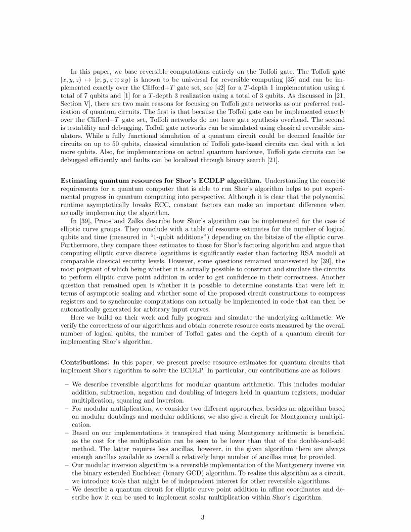
In this paper, we base reversible computations entirely on the Toffoli gate. The Toffoli gate|x, y, z〉 7→ |x, y, z ⊕ xy〉 is known to be universal for reversible computing [35] and can be im-plemented exactly over the Clifford+T gate set, see [42] for a T -depth 1 implementation using atotal of 7 qubits and [1] for a T -depth 3 realization using a total of 3 qubits. As discussed in [21,Section V], there are two main reasons for focusing on Toffoli gate networks as our preferred real-ization of quantum circuits. The first is that because the Toffoli gate can be implemented exactlyover the Clifford+T gate set, Toffoli networks do not have gate synthesis overhead. The secondis testability and debugging. Toffoli gate networks can be simulated using classical reversible sim-ulators. While a fully functional simulation of a quantum circuit could be deemed feasible forcircuits on up to 50 qubits, classical simulation of Toffoli gate-based circuits can deal with a lotmore qubits. Also, for implementations on actual quantum hardware, Toffoli gate circuits can bedebugged efficiently and faults can be localized through binary search [21].

Estimating quantum resources for Shor’s ECDLP algorithm. Understanding the concreterequirements for a quantum computer that is able to run Shor’s algorithm helps to put experi-mental progress in quantum computing into perspective. Although it is clear that the polynomialruntime asymptotically breaks ECC, constant factors can make an important difference whenactually implementing the algorithm.

In [39], Proos and Zalka describe how Shor’s algorithm can be implemented for the case ofelliptic curve groups. They conclude with a table of resource estimates for the number of logicalqubits and time (measured in “1-qubit additions”) depending on the bitsize of the elliptic curve.Furthermore, they compare these estimates to those for Shor’s factoring algorithm and argue thatcomputing elliptic curve discrete logarithms is significantly easier than factoring RSA moduli atcomparable classical security levels. However, some questions remained unanswered by [39], themost poignant of which being whether it is actually possible to construct and simulate the circuitsto perform elliptic curve point addition in order to get confidence in their correctness. Anotherquestion that remained open is whether it is possible to determine constants that were left interms of asymptotic scaling and whether some of the proposed circuit constructions to compressregisters and to synchronize computations can actually be implemented in code that can then beautomatically generated for arbitrary input curves.

Here we build on their work and fully program and simulate the underlying arithmetic. Weverify the correctness of our algorithms and obtain concrete resource costs measured by the overallnumber of logical qubits, the number of Toffoli gates and the depth of a quantum circuit forimplementing Shor’s algorithm.

Contributions. In this paper, we present precise resource estimates for quantum circuits thatimplement Shor’s algorithm to solve the ECDLP. In particular, our contributions are as follows:

– We describe reversible algorithms for modular quantum arithmetic. This includes modularaddition, subtraction, negation and doubling of integers held in quantum registers, modularmultiplication, squaring and inversion.

– For modular multiplication, we consider two different approaches, besides an algorithm basedon modular doublings and modular additions, we also give a circuit for Montgomery multipli-cation.

– Based on our implementations it transpired that using Montgomery arithmetic is beneficialas the cost for the multiplication can be seen to be lower than that of the double-and-addmethod. The latter requires less ancillas, however, in the given algorithm there are alwaysenough ancillas available as overall a relatively large number of ancillas must be provided.

– Our modular inversion algorithm is a reversible implementation of the Montgomery inverse viathe binary extended Euclidean (binary GCD) algorithm. To realize this algorithm as a circuit,we introduce tools that might be of independent interest for other reversible algorithms.

– We describe a quantum circuit for elliptic curve point addition in affine coordinates and de-scribe how it can be used to implement scalar multiplication within Shor’s algorithm.

3

– We have implemented all of the above algorithms in F# within the framework of the quan-tum computing software tool suite LIQUi|〉 [52] and have simulated and tested all of thesealgorithms for real-world parameters of up to 521 bits4.

– Derived from our implementation, we present concrete resource estimates for the total numberof qubits, the number of Toffoli gates and the depth of the Toffoli gate networks to realize Shor’salgorithm and its subroutines. We compare the quantum resources for solving the ECDLP tothose required in Shor’s factoring algorithm that were obtained in the recent work [21].

Results. Our implementation realizes a reversible circuit for controlled elliptic curve point ad-dition on an elliptic curve defined over a field of prime order with n bits and needs at most9n + 2dlog2(n)e + 10 qubits. An interpolation of the data points for the number of Toffoli gatesshows that the quantum circuit can be implemented with at most roughly 224n2 log2(n) + 2045n2

Toffoli gates. For Shor’s full algorithm, the point addition needs to be run 2n times sequen-tially and does not need additional qubits. The overall number of Toffoli gates is thus about448n3 log2(n) + 4090n3. For example, our simulation of the point addition quantum circuit for theNIST standardized curve P-256 needs 2330 logical qubits and the full Shor algorithm would needabout 1.26 · 1011 Toffoli gates. In comparison, Shor’s factoring algorithm for a 3072-bit modulusneeds 6146 qubits and 1.86 · 1013 Toffoli gates5, which aligns with results by Proos and Zalkashowing that it is easier to break ECC than RSA at comparable classical security.

Our estimates provide a data point that allows a better understanding of the requirements torun Shor’s quantum ECDLP algorithm and we hope that they will serve as a basis to make betterpredictions about the time horizon until which elliptic curve cryptography can still be consideredsecure. Besides helping to gain a better understanding of the post-quantum (in-) security of ellipticcurve cryptosystems, we hope that our reversible algorithms (and their LIQUi|〉 implementations)for modular arithmetic and the elliptic curve group law are of independent interest to some, andmight serve as building blocks for other quantum algorithms.

2 Elliptic curves and Shor’s algorithm

This section provides some background on elliptic curves over finite fields, the elliptic curve discretelogarithm problem (ECDLP) and Shor’s quantum algorithm to solve the ECDLP. Throughout,we restrict to the case of curves defined over prime fields of large characteristic.

2.1 Elliptic curves and the ECDLP

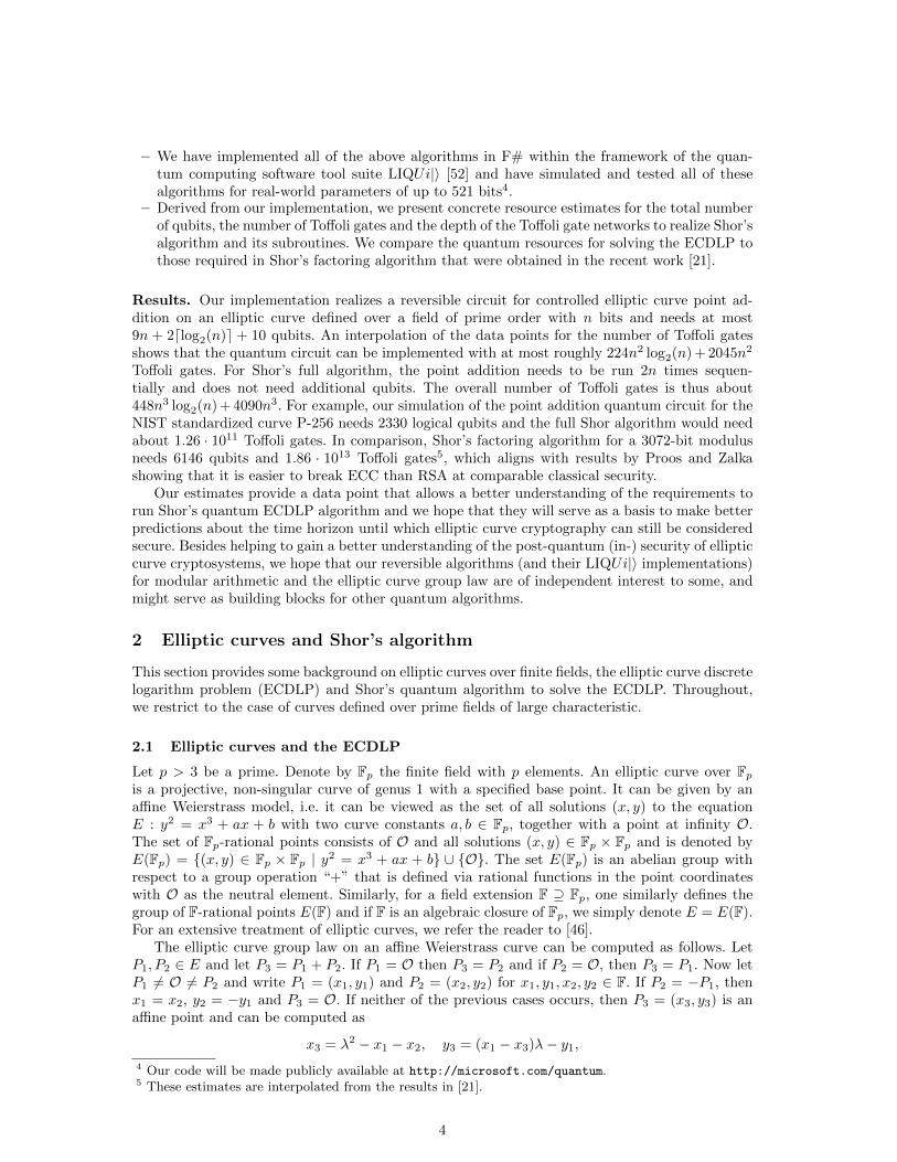
Let p > 3 be a prime. Denote by Fp the finite field with p elements. An elliptic curve over Fpis a projective, non-singular curve of genus 1 with a specified base point. It can be given by anaffine Weierstrass model, i.e. it can be viewed as the set of all solutions (x, y) to the equationE : y2 = x3 + ax + b with two curve constants a, b ∈ Fp, together with a point at infinity O.The set of Fp-rational points consists of O and all solutions (x, y) ∈ Fp × Fp and is denoted byE(Fp) = {(x, y) ∈ Fp × Fp | y2 = x3 + ax + b} ∪ {O}. The set E(Fp) is an abelian group withrespect to a group operation “+” that is defined via rational functions in the point coordinateswith O as the neutral element. Similarly, for a field extension F ⊇ Fp, one similarly defines thegroup of F-rational points E(F) and if F is an algebraic closure of Fp, we simply denote E = E(F).For an extensive treatment of elliptic curves, we refer the reader to [46].

The elliptic curve group law on an affine Weierstrass curve can be computed as follows. LetP1, P2 ∈ E and let P3 = P1 + P2. If P1 = O then P3 = P2 and if P2 = O, then P3 = P1. Now letP1 6= O 6= P2 and write P1 = (x1, y1) and P2 = (x2, y2) for x1, y1, x2, y2 ∈ F. If P2 = −P1, thenx1 = x2, y2 = −y1 and P3 = O. If neither of the previous cases occurs, then P3 = (x3, y3) is anaffine point and can be computed as

x3 = λ2 − x1 − x2, y3 = (x1 − x3)λ− y1,4 Our code will be made publicly available at http://microsoft.com/quantum.5 These estimates are interpolated from the results in [21].

4

where λ = y2−y1x2−x1

if P1 6= P2, i.e. x1 6= x2, and λ =3x2

1+a2y1

if P1 = P2. For a positive integer m,

denote by [m]P the m-fold sum of P , i.e. [m]P = P + · · ·+P , where P occurs m times. Extendedto all m ∈ Z by [0]P = O and [−m]P = [m](−P ), the map [m] : E → E,P 7→ [m]P is calledthe multiplication-by-m map or simply scalar multiplication by m. Scalar multiplication (or groupexponentiation in the multiplicative setting) is one of the main ingredients for discrete-logarithm-based cryptographic protocols. It is also an essential operation in Shor’s ECDLP algorithm. Theorder ord(P ) of a point P is the smallest positive integer r such that [r]P = O.

Curves that are most widely used in cryptography are defined over large prime fields. Oneworks in a cyclic subgroup of E(Fp) of large prime order r, where #E(Fp) = h · r. The grouporder can be written as #E(Fp) = p+ 1− t, where t is called the trace of Frobenius and the Hassebound ensures that |t| ≤ 2

√p. Thus #E(Fp) and p are of roughly the same size. The most efficient

instantiations of ECC are achieved for small cofactors h. For example, the above mentioned NISTcurves have prime order, i.e. h = 1, and Curve25519 has cofactor h = 8. Let P ∈ E(Fp) be anFp-rational point on E of order r and let Q ∈ 〈P 〉 be an element of the cyclic subgroup generatedby P . The Elliptic Curve Discrete Logarithm Problem (ECDLP) is the problem to find the integerm ∈ Z/rZ such that Q = [m]P . The bit security of an elliptic curve is estimated by extrapolatingthe runtime of the most efficient algorithms for the ECDLP.

The currently best known classical algorithms to solve the ECDLP are based on parallelizedversions of Pollard’s rho algorithm [37, 51, 38]. When working in a group of order n, the expectedrunning time for solving a single ECDLP is (

√π/2 + o(1))

√n group operations based on the

birthday paradox. This is exponential in the input size log(n). See [16] for further details and [6]for a concrete, implementation-based security assessment.

2.2 Shor’s quantum algorithm for solving the ECDLP

In [44], Shor presented two polynomial time quantum algorithms, one for factoring integers, theother for computing discrete logarithms in finite fields. The second one can naturally be appliedfor computing discrete logarithms in the group of points on an elliptic curve defined over a finitefield.

We are given an instance of the ECDLP as described above. Let P ∈ E(Fp) be a fixed generatorof a cyclic subgroup of E(Fp) of known order ord(P ) = r, let Q ∈ 〈P 〉 be a fixed element in thesubgroup generated by P ; our goal is to find the unique integer m ∈ {1, . . . , r} such that Q = [m]P .Shor’s algorithm proceeds as follows. First, two registers of length n + 1 qubits6 are created andeach qubit is initialized in the |0〉 state. Then a Hadamard transform H is applied to each qubit,

resulting in the state 12n+1

∑2n+1−1k,`=0 |k, `〉. Next, conditioned on the content of the register holding

the label k or `, we add the corresponding multiple of P and Q, respectively, i. e., we implementthe map

1

2n+1

2n+1−1∑k,`=0

|k, `〉 7→ 1

2n+1

2n+1−1∑k,`=0

|k, `〉 |[k]P + [`]Q〉 .

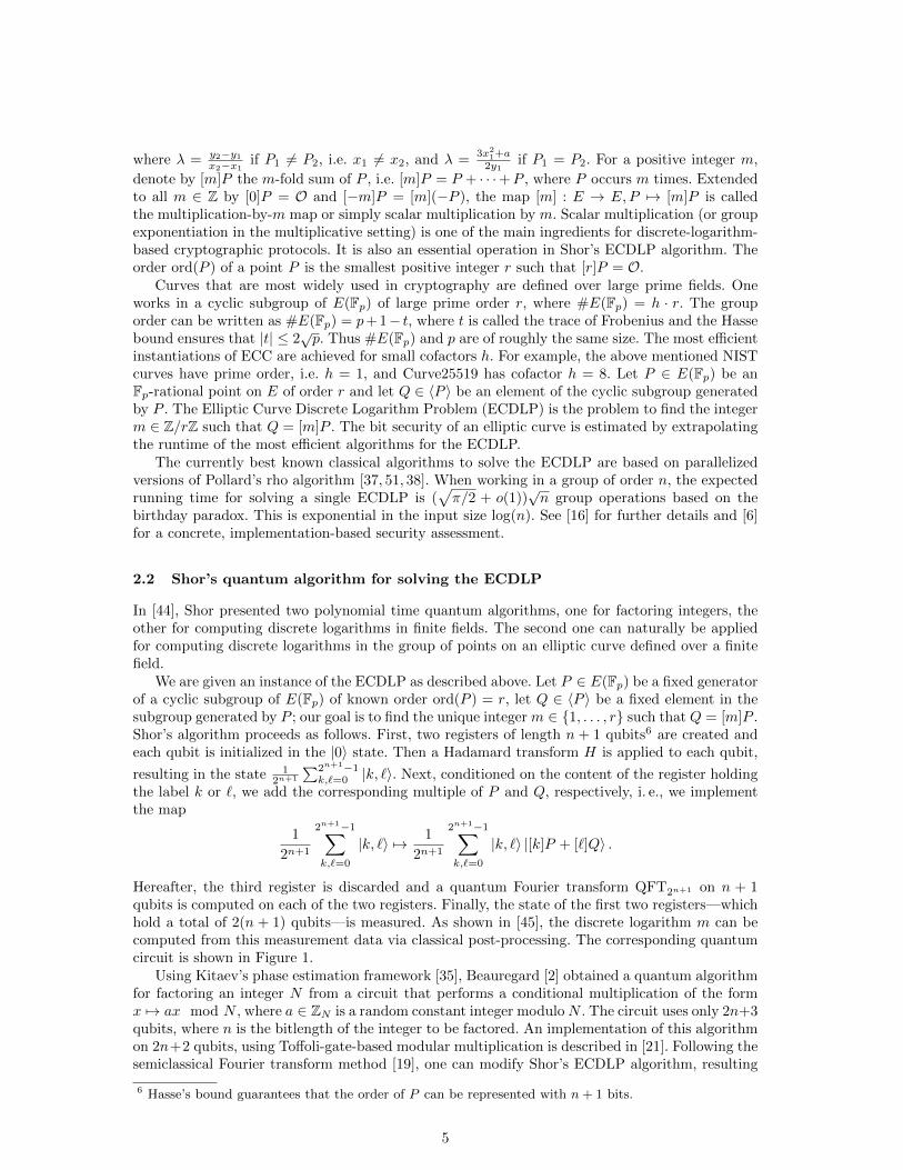
Hereafter, the third register is discarded and a quantum Fourier transform QFT2n+1 on n + 1qubits is computed on each of the two registers. Finally, the state of the first two registers—whichhold a total of 2(n + 1) qubits—is measured. As shown in [45], the discrete logarithm m can becomputed from this measurement data via classical post-processing. The corresponding quantumcircuit is shown in Figure 1.

Using Kitaev’s phase estimation framework [35], Beauregard [2] obtained a quantum algorithmfor factoring an integer N from a circuit that performs a conditional multiplication of the formx 7→ ax mod N , where a ∈ ZN is a random constant integer moduloN . The circuit uses only 2n+3qubits, where n is the bitlength of the integer to be factored. An implementation of this algorithmon 2n+2 qubits, using Toffoli-gate-based modular multiplication is described in [21]. Following thesemiclassical Fourier transform method [19], one can modify Shor’s ECDLP algorithm, resulting

6 Hasse’s bound guarantees that the order of P can be represented with n+ 1 bits.

5

in the circuit shown in Figure 2. The phase shift matrices Ri =(

1 0

0 eiθk

), θk = −π

∑k−1j=0 2k−jµj ,

depend on all previous measurement outcomes µj ∈ {0, 1}, j ∈ {0, . . . , k − 1}.

|0〉 H . . . . . . •

QFT2n+1

......

...

|0〉 H . . . • . . .

|0〉 H . . . • . . .

|0〉 H . . . • . . .

QFT2n+1

......

...

|0〉 H • . . . . . .

|0〉 H • . . . . . .

|O〉 /2n +P +[2]P . . . +[2n]P +Q +[2]Q . . . +[2n]Q

Fig. 1: Shor’s algorithm to compute the discrete logarithm in the subgroup of an elliptic curve generatedby a point P . The input to the problem is a point Q, and the task is to find m ∈ {1, . . . , ord(P )} such thatQ = [m]P . The circuit naturally decomposes into three parts, namely (i) the Hadamard layer on the left,(ii) a double scalar multiplication (in this figure implemented as a cascade of conditional point additions),and (iii) the quantum Fourier transform QFT and subsequent measurement in the standard basis whichis performed at the end.

µ0 µ1 µ2n+1

|0〉 H • H |0〉 H • R1 H . . . |0〉 H • R2n+1 H

|O〉 /2n +P +[2]P . . . +[2n]Q

Fig. 2: Shor’s algorithm to compute the discrete logarithm in the subgroup of an elliptic curve generatedby a point P , analogous to the algorithms from [2, 19, 21]. The gates Rk are phase shift gates givenby diag(1, eiθk ), where θk = −π

∑k−1j=0 2k−jµj and the sum runs over all previous measurements j with

outcome µj ∈ {0, 1}. In contrast to the circuit in Figure 1 only one additional qubit is needed besidesqubits required to represent and add the elliptic curve points.

3 Reversible modular arithmetic

Shor’s algorithm for factoring actually only requires modular multiplication of a quantum integerwith classically known constants. In contrast, the elliptic curve discrete logarithm algorithm re-quires elliptic curve scalar multiplications to compute [k]P + [`]Q for a superposition of values forthe scalars k and `. These scalar multiplications are comprised of elliptic curve point additions,which in turn consist of a sequence of modular operations on the coordinates of the elliptic curvepoints. This requires the implementation of full modular arithmetic, which means that one needsto add and multiply two integers held in quantum registers modulo the constant integer modulusp.

This section presents quantum circuits for reversible modular arithmetic on n-bit integers thatare held in quantum registers. We provide circuit diagrams for the modular operations, in which

6

black triangles on the right side of gate symbols indicate qubit registers that are modified andhold the result of the computation. Essential tools for implementing modular arithmetic are integeraddition and bit shift operations on integers, which we describe first.

3.1 Integer addition and binary shifts

The algorithms for elliptic curve point addition as described below need integer addition andsubtraction in different variants: standard integer addition and subtraction of two n-bit integers,addition and subtraction of a classical constant integer, as well as controlled versions of those.

For adding two integers, we take the quantum circuit described by Takahashi et al. [49]. Thecircuit works on two registers holding the input integers, the first of size n qubits and the secondof size n+1 qubits. It operates in place, i.e. the contents of the second register are replaced to holdthe sum of the inputs storing a possible carry bit in the additionally available qubit. To obtaina subtraction circuit, we implement an inverse version of this circuit. The carry bit in this caseindicates whether the result of the subtraction is negative. Controlled versions of these circuitscan be obtained by using partial reflection symmetry to save controls, which compares favorablyto a generic version where simply all gates are controlled. For the constant addition circuits, wetake the algorithms described in [21]. Binary doubling and halving circuits are needed for theMontgomery multiplication and inversion algorithms. They are implemented essentially as cyclicbit shifts realized by sequences of symmetric bit swap operations built from CNOT gates.

3.2 Modular addition and doubling

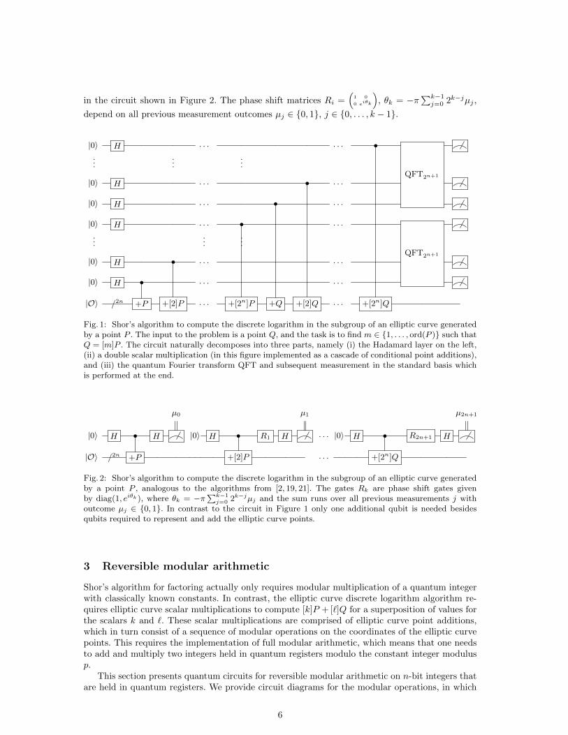
We now turn to modular arithmetic. The circuit shown in Figure 3 computes a modular additionof two integers x and y held in n-qubit quantum registers |x〉 and |y〉, modulo the constant integermodulus p. It performs the operation in place |x〉 |y〉 7→ |x〉 |(x+ y) mod p〉 and replaces the secondinput with the result. It uses quantum circuits for plain integer addition and constant additionand subtraction of the modulus. It uses two auxiliary qubits, one of which is used as an ancillaqubit in the constant addition and subtraction and can be in an unknown state to which it willbe returned at the end of the circuit. The other qubit stores the bit that determines whether amodular reduction in form of a modulus subtraction actually needs to be performed or not. Itis uncomputed at the end by a strict comparison circuit between the result and the first input.Modular subtraction is implemented by reversing the circuit.

The modular doubling circuit for a constant odd integer modulus p in Figure 4 follows the sameprinciple. There are two changes that make it more efficient than the addition circuit. First of allit works in place on only one n-qubit input integer |x〉, it computes |x〉 7→ |2x mod p〉. Thereforeit uses only n+ 2 qubits. The first integer addition in the modular adder circuit is replaced by amore efficient multiplication by 2 implemented via a cyclic bit shift as described in the previoussubsection. Since we assume that the modulus p is odd in this circuit, the auxiliary reduction

|x〉 /n

+ I

I

>

I

|x〉

|y〉 /n

−p

I

I

+p I |(x+ y) mod p〉

|0〉 • |0〉

|g〉 +p |g〉

Fig. 3: add modp: Quantum circuit for in-place modular addition |x〉 |y〉 7→ |x〉 |(x+ y) mod p〉. The regis-ters |x〉, |y〉 consist of n logical qubits each. The circuit uses integer addition +, addition +p and subtraction−p of the constant modulus p, and strict comparison of two n-bit integers in the registers |x〉 and |y〉,where the output bit flips the carry qubit in the last register. The constant adders use an ancilla qubitin an unknown state |g〉, which is returned to the same state at the end of the circuit. To implementcontrolled modular addition ctrl add modp, one simply controls all operations in this circuit.

7

|x0〉

·2

I

I−p

I

I+p

I

I

|(2x mod p)0〉

|x1,...,n−1〉 /n−1∣∣(2x mod p)1,...,(n−1)

⟩|0〉 • |0〉

|g〉 +p |g〉

Fig. 4: dbl modp: Quantum circuit for in-place modular doubling |x〉 7→ |2x mod p〉 for an odd constantmodulus p. The registers |x〉 consists of n logical qubits, the circuit diagram represents the least significantbit separately. The circuit uses a binary doubling operation ·2 and addition +p and subtraction −p of theconstant modulus p. The constant adders use an ancilla qubit in an unknown state |g〉, which is returnedto the same state at the end of the circuit.

qubit can be uncomputed by checking whether the least significant bit of the result is 0 or 1. Asubtraction of the modulus has taken place if, and only if this bit is 1.

For adding a classical constant to a quantum register modulo a classical constant modulus,we use the in-place modular addition circuit described in [21, Section II]. The circuit operateson the n-bit input and requires only 1 ancilla qubit initialized in the state |0〉 and n − 1 dirtyancillas that are given in an unknown state and will be returned in the same state at the end ofthe computation.

3.3 Modular multiplication

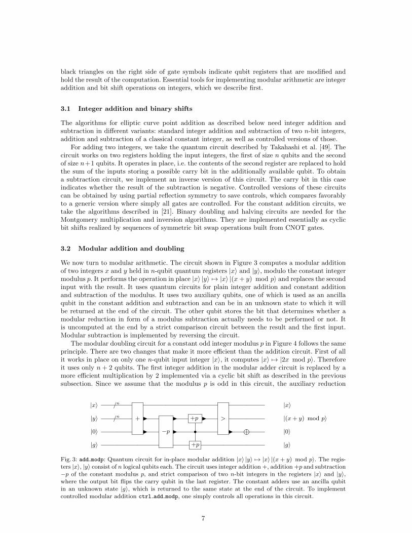
Multiplication by modular doubling and addition. Modular multiplication can be computedby repeated modular doublings and conditional modular additions. Figure 5 shows a circuit thatcomputes the product z = x ·y mod p for constant modulus p as described by Proos and Zalka [39,Section 4.3.2] by using a simple expansion of the product along a binary decomposition of the firstmultiplicand, i.e.

x · y =

n−1∑i=0

xi2i · y = x0y + 2(x1y + 2(x2y + · · ·+ 2(xn−2y + 2(xn−1y)) . . . )).

The circuit runs on 3n+ 2 qubits, 2n of which are used to store the inputs, n to accumulate theresult and 2 ancilla qubits are needed for the modular addition and doubling operations, one ofwhich can be dirty. The latter could be taken to be one of the xi, for example x0 except in thelast step, when the modular addition gate is conditioned on x0. For simplicity, we assume it to bea separate qubit.

Figure 6 shows the corresponding specialization to compute a square z = x2 mod p. It uses2n+ 3 qubits by removing the n qubits for the second input multiplicand, and adding one ancillaqubit, which is used in round i to copy out the current bit xi of the input in order to add x to theaccumulator conditioned on the value of xi.

Montgomery multiplication In classical applications, Montgomery multiplication [33] is oftenthe most efficient choice for modular multiplication if the modulus does not have a special shapesuch as being close to a power of 2. Here, we explore it as an alternative to the algorithm usingmodular doubling and addition as described above.

In [33], Montgomery introduced a representation for an integer modulo p he called a p-residuethat is now called the Montgomery representation. Let R > p be an integer radix coprime to p. Aninteger a modulo p is represented by the Montgomery representation aR mod p. The Montgomeryreduction algorithm takes as input an integer 0 ≤ c < Rp and computes cR−1 mod p. Thus giventwo integers aR mod p and bR mod p in Montgomery representation, applying the Montgomeryreduction to their product yields the Montgomery representation (ab)R mod p of the product.If R is a power of 2, one can interleave the Montgomery reduction with school-book multiplica-tion, obtaining a combined Montgomery multiplication algorithm. The division operations usually

8

|x0〉 . . . • |x0〉|x1〉 . . . • |x1〉...

......

......

|xn−3〉 • . . . |xn−3〉|xn−2〉 • . . . |xn−2〉|xn−1〉 • . . . |xn−1〉|y〉 /n

+ I + I + I

. . .

+ I + I

|y〉

|0〉 /n

dblI

dblI

dblI . . .

dblI |x · y mod p〉

|0g〉 /2 . . . |0g〉

Fig. 5: mul modp: Quantum circuit for modular multiplication |x〉 |y〉 |0〉 7→ |x〉 |y〉 |x · y mod p〉 built frommodular doublings dbl ← dbl modp and controlled modular additions + ← ctrl add modp. The registers|xi〉 hold single logical qubits, |y〉 and |0〉 hold n logical qubits. The two ancilla qubits |0g〉 are the onesneeded in the modular addition and doubling circuits, the second one can be in an unknown state to whichit will be returned.

|0〉 • • . . . • |0〉

|x0〉

+ +

. . . •

+

• |x0〉

|x1〉 . . . • |x1〉...

......

...

|xn−3〉 . . . |xn−3〉

|xn−2〉 • • . . . |xn−2〉

|xn−1〉 • • . . . |xn−1〉

|0〉 /n

dblI

dblI . . .

dblI

∣∣x2 mod p⟩

|0g〉 /2 . . . |0g〉

Fig. 6: squ modp: Quantum circuit for modular squaring |x〉 |0〉 7→ |x〉∣∣x2 mod p

⟩built from modular

doublings dbl← dbl modp and controlled modular additions +← ctrl add modp. The registers |xi〉 holdsingle logical qubits, |0〉 holds n logical qubits. The two ancilla qubits |0g〉 are the ones needed in themodular addition and doubling circuits, the second one can be in an unknown state to which it will bereturned.

needed for computing remainders are replaced by binary shifts in each round of the multiplicationalgorithm.

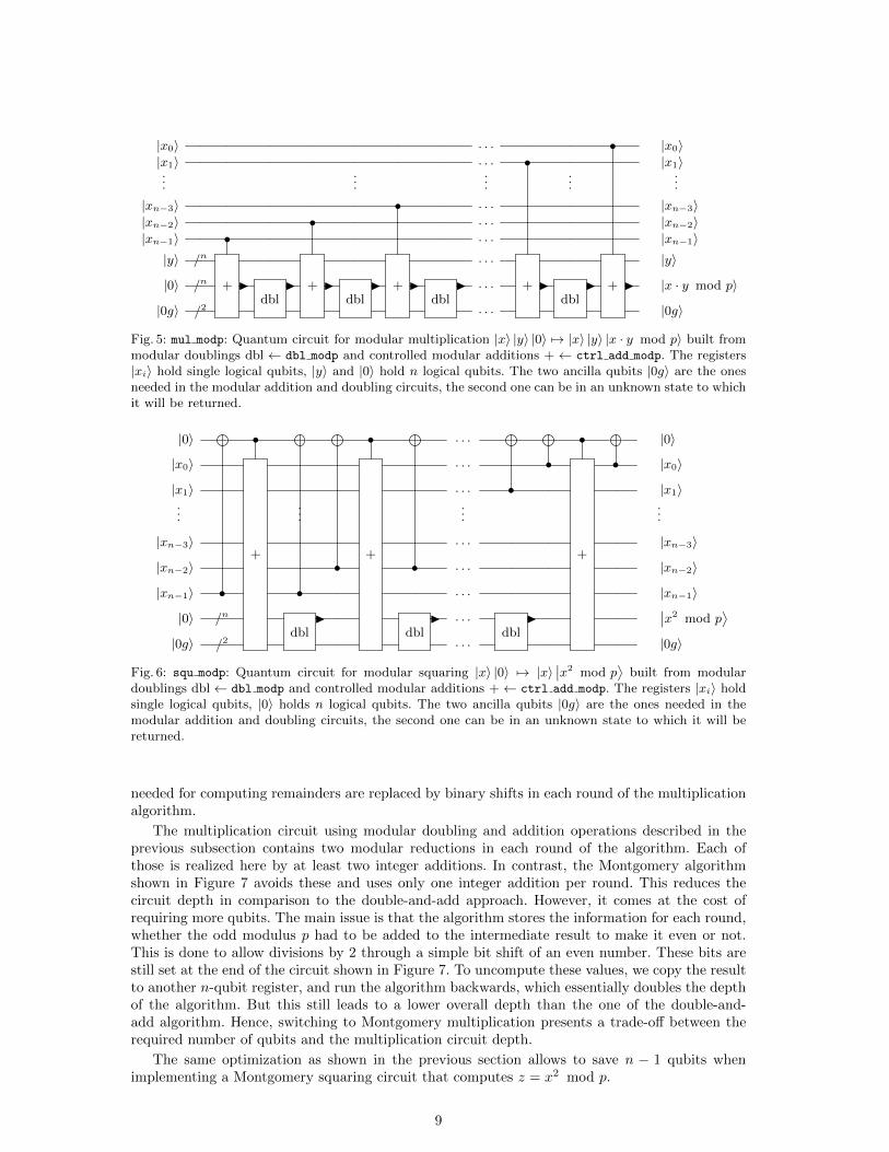
The multiplication circuit using modular doubling and addition operations described in theprevious subsection contains two modular reductions in each round of the algorithm. Each ofthose is realized here by at least two integer additions. In contrast, the Montgomery algorithmshown in Figure 7 avoids these and uses only one integer addition per round. This reduces thecircuit depth in comparison to the double-and-add approach. However, it comes at the cost ofrequiring more qubits. The main issue is that the algorithm stores the information for each round,whether the odd modulus p had to be added to the intermediate result to make it even or not.This is done to allow divisions by 2 through a simple bit shift of an even number. These bits arestill set at the end of the circuit shown in Figure 7. To uncompute these values, we copy the resultto another n-qubit register, and run the algorithm backwards, which essentially doubles the depthof the algorithm. But this still leads to a lower overall depth than the one of the double-and-add algorithm. Hence, switching to Montgomery multiplication presents a trade-off between therequired number of qubits and the multiplication circuit depth.

The same optimization as shown in the previous section allows to save n − 1 qubits whenimplementing a Montgomery squaring circuit that computes z = x2 mod p.

9

|x0〉 • . . . |x0〉|x1〉 • . . . |x1〉...

......

......

|xn−1〉 . . . • |xn−1〉|y〉 /

+I

I

I

+I

I

I

. . .

+I

I

I

|y〉

|0〉

+p

I

I

I

/2

I

I

I+p

I

I

I

/2

I

I

I

. . .

+p

I

I

I

/2

I

I

I−p

I

I

I

• |c〉

|0..0〉 / . . .

+p

I

I

|z1,...,n−1〉

|0〉 • • . . . • |z0〉

|g〉 . . . |g〉

|0〉 • . . . |m0〉

|0〉 • . . . |m1〉...

......

......

|0〉 . . . • |mn−1〉

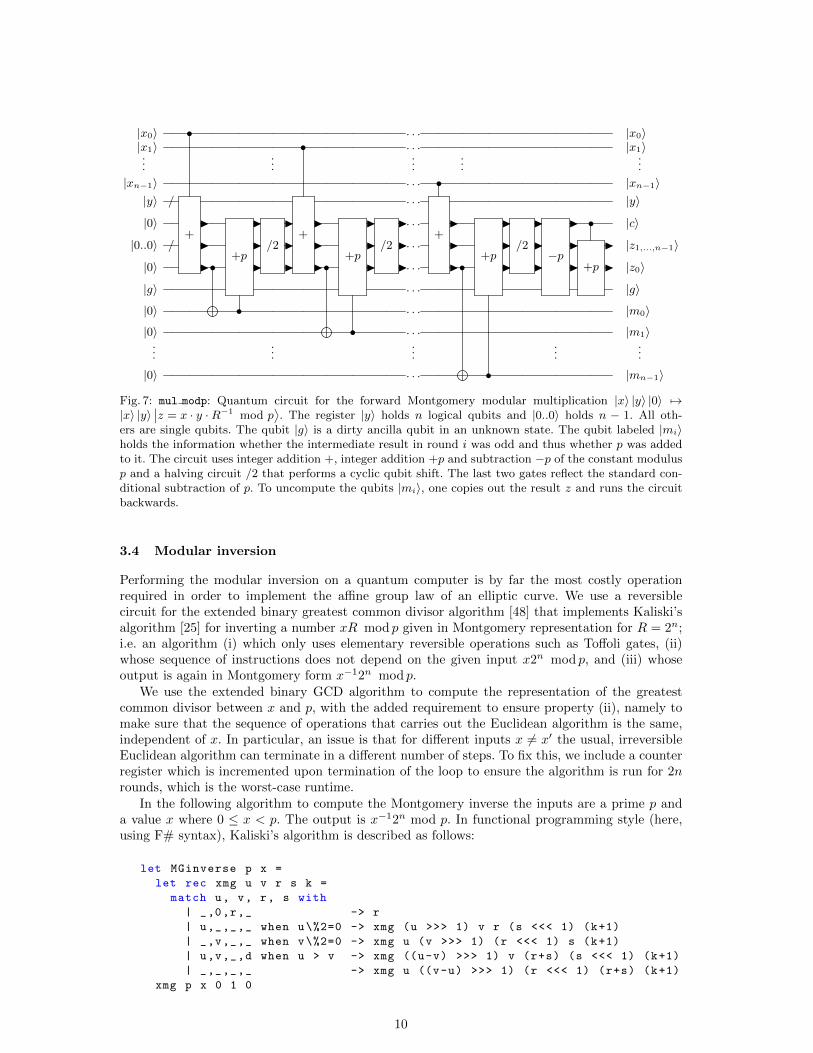
Fig. 7: mul modp: Quantum circuit for the forward Montgomery modular multiplication |x〉 |y〉 |0〉 7→|x〉 |y〉

∣∣z = x · y ·R−1 mod p⟩. The register |y〉 holds n logical qubits and |0..0〉 holds n − 1. All oth-

ers are single qubits. The qubit |g〉 is a dirty ancilla qubit in an unknown state. The qubit labeled |mi〉holds the information whether the intermediate result in round i was odd and thus whether p was addedto it. The circuit uses integer addition +, integer addition +p and subtraction −p of the constant modulusp and a halving circuit /2 that performs a cyclic qubit shift. The last two gates reflect the standard con-ditional subtraction of p. To uncompute the qubits |mi〉, one copies out the result z and runs the circuitbackwards.

3.4 Modular inversion

Performing the modular inversion on a quantum computer is by far the most costly operationrequired in order to implement the affine group law of an elliptic curve. We use a reversiblecircuit for the extended binary greatest common divisor algorithm [48] that implements Kaliski’salgorithm [25] for inverting a number xR mod p given in Montgomery representation for R = 2n;i.e. an algorithm (i) which only uses elementary reversible operations such as Toffoli gates, (ii)whose sequence of instructions does not depend on the given input x2n mod p, and (iii) whoseoutput is again in Montgomery form x−12n mod p.

We use the extended binary GCD algorithm to compute the representation of the greatestcommon divisor between x and p, with the added requirement to ensure property (ii), namely tomake sure that the sequence of operations that carries out the Euclidean algorithm is the same,independent of x. In particular, an issue is that for different inputs x 6= x′ the usual, irreversibleEuclidean algorithm can terminate in a different number of steps. To fix this, we include a counterregister which is incremented upon termination of the loop to ensure the algorithm is run for 2nrounds, which is the worst-case runtime.

In the following algorithm to compute the Montgomery inverse the inputs are a prime p anda value x where 0 ≤ x < p. The output is x−12n mod p. In functional programming style (here,using F# syntax), Kaliski’s algorithm is described as follows:

let MGinverse p x =

let rec xmg u v r s k =

match u, v, r, s with

| _,0,r,_ -> r

| u,_,_,_ when u\%2=0 -> xmg (u >>> 1) v r (s <<< 1) (k+1)

| _,v,_,_ when v\%2=0 -> xmg u (v >>> 1) (r <<< 1) s (k+1)

| u,v,_,d when u > v -> xmg ((u-v) >>> 1) v (r+s) (s <<< 1) (k+1)

| _,_,_,_ -> xmg u ((v-u) >>> 1) (r <<< 1) (r+s) (k+1)

xmg p x 0 1 0

10

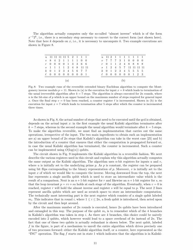
The algorithm actually computes only the so-called “almost inverse” which is of the formx−12k, i.e., there is a secondary step necessary to convert to the correct form (not shown here).Note that here k depends on x, i.e., it is necessary to uncompute k. Two example executions areshown in Figure 8.

u 11 11 11 11 5 2 1 1 1v 8 4 2 1 1 1 1 0 0r 0 0 0 0 1 3 3 6 6s 1 1 1 1 2 4 8 11 11k 0 1 2 3 4 5 6 7 7` 0 0 0 0 0 0 0 0 1

u 11 2 1 1 1 1 1 1 1v 7 7 7 3 1 0 0 0 0r 0 1 1 2 4 8 8 8 8s 1 2 4 5 7 11 11 11 11k 0 1 2 3 4 5 5 5 5` 0 0 0 0 0 0 1 2 3

(a) (b)

Fig. 8: Two example runs of the reversible extended binary Euclidean algorithm to compute the Mont-gomery inverse modulo p = 11. Shown in (a) is the execution for input x = 8 which leads to termination ofthe usual irreversible algorithm after k = 7 steps. The algorithm is always executed for 2n rounds, wheren is the bit-size of p which is an upper bound on the maximum number of steps required for general inputx. Once the final step v = 0 has been reached, a counter register ` is incremented. Shown in (b) is theexecution for input x = 7 which leads to termination after 5 steps after which the counter is incrementedthree times.

As shown in Fig. 8, the actual number of steps that need to be executed until the gcd is obtained,depends on the actual input x: in the first example the usual Kaliski algorithm terminates afterk = 7 steps, whereas in the second example the usual algorithm would terminate after k = 5 steps.To make the algorithm reversible, we must find an implementation that carries out the sameoperations, irrespective of the input. The two main ingredients to obtain such an implementationare a) an upper bound of 2n steps that Kaliski’s algorithm can take in the worst case [25] and b)the introduction of a counter that ensures that either the computation is propagated forward or,in case the usual Kaliski algorithm has terminated, the counter is incremented. Such a countercan be implemented using O(log(n)) qubits.

The circuit shown in Fig. 9 implements the Kaliski algorithm in a reversible fashion. We nextdescribe the various registers used in this circuit and explain why this algorithm actually computesthe same output as the Kaliski algorithm. The algorithm uses n-bit registers for inputs u and v,where u is initially set to the underlying prime p. As p is constant, the register can be preparedusing bit flips corresponding to the binary representation of p. Moreover, v is initially set to theinput x of which we would like to compute the inverse. Moving downward from the top, the nextline represents a single ancilla qubit which is used to store an intermediate value which is theresult of a comparison. Next is an n+1-bit register for r and likewise an n+1-bit register for s, sothat the loop invariant p = rv+su holds at each stage of the algorithm. Eventually, when v = 0 isreached, register r will hold the almost inverse and register s will be equal to p. The next 2 linesrepresent ancilla qubits which are used as scratch space to store an intermediate computation.The technically most interesting part is the next register which consists of a single qubit labeledmi. This indicates that in round i, where 1 ≤ i ≤ 2n, a fresh qubit is introduced, then acted uponby the circuit and then kept around.

After the maximum number of 2n rounds is executed, hence 2n qubits have been introducedand entangled in this way. The purpose of the qubit mi is to remember which of the 4 branchesin Kaliski’s algorithm was taken in step i. As there are 4 branches, this choice could be naivelyencoded into 2 qubits, which however would lead to a space overhead of 4n instead of 2n. Thefact that one of these two qubits is actually redundant is shown below. The next qubit, labeledf in the figure, is part of a mechanism to unroll the entire algorithm which drives precisely oneof two processes forward: either the Kaliski algorithm itself, or a counter, here represented as the“INC” operation. The flag f starts out in state 1 which indicates that the algorithm is in Kaliski-

11

|u〉 /n

− I

I

+ I

I

/2

−I /2

−I

|u〉

|v〉 /n /2 /2 |v〉

|0〉 • |0〉

|s〉 /n ·2+

I

·2+

I |s〉

|r〉 /n ·2 ·2 • |r〉

|0〉 |0〉

|0〉 • • • • • |0〉

|mi〉 • • • • • |mi〉

|f〉 • |f〉

|k〉 /l • INC |k〉

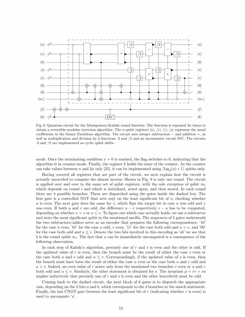
Fig. 9: Quantum circuit for the Montgomery-Kaliski round function. The function is repeated 2n times toobtain a reversible modular inversion algorithm. The n-qubit registers |u〉, |v〉, |r〉, |s〉 represent the usualcoefficients in the binary Euclidean algorithm. The circuit uses integer subtraction − and addition +, aswell as multiplication and division by 2 functions ·2 and /2 and an incrementer circuit INC. The circuits·2 and /2 are implemented as cyclic qubit shifts.

mode. Once the terminating condition v = 0 is reached, the flag switches to 0, indicating that thealgorithm is in counter-mode. Finally, the register k holds the state of the counter. As the countercan take values between n and 2n only [25], it can be implemented using dlog2(n)+1e qubits only.

Having covered all registers that are part of the circuit, we next explain how the circuit isactually unraveled to compute the almost inverse. Shown in Fig. 9 is only one round. The circuitis applied over and over to the same set of qubit registers, with the sole exception of qubit mi

which depends on round i and which is initialized, acted upon, and then stored. In each roundthere are 4 possible branches. These are dispatched using the gates inside the dashed box. Thefirst gate is a controlled NOT that acts only on the least significant bit of u, checking whetheru is even. The next gate does the same for v, which flips the target bit in case u was odd and vwas even. If both u and v are odd, the difference u − v respectively v − u has to be computed,depending on whether u > v or u ≤ v. To figure out which case actually holds, we use a subtractorand store the most significant qubit in the mentioned ancilla. The sequences of 5 gates underneaththe two subtractors/adders serve as an encoder that prepares the following correspondence: ‘10’for the case u even, ’01’ for the case u odd, v even, ’11’ for the case both odd and u > v, and ’00’for the case both odd and u ≤ v. Denote the two bits involved in this encoding as ’ab’ we see thatb is the round qubit mi. The fact that a can be immediately uncomputed is a consequence of thefollowing observation.

In each step of Kaliski’s algorithm, precisely one of r and s is even and the other is odd. Ifthe updated value of r is even, then the branch must be the result of either the case v even orthe case both u and v odd and u ≤ v. Correspondingly, if the updated value of s is even, thenthe branch must have been the result of either the case u even or the case both u and v odd andu > v. Indeed, an even value of r arises only from the mentioned two branches v even or u and vboth odd and u ≤ v. Similarly, the other statement is obtained for s. The invariant p = rv + suimplies inductively that precisely one of r and s is even and the other henceforth must be odd.

Coming back to the dashed circuit, the next block of 6 gates is to dispatch the appropriatecase, depending on the 2 bits a and b, which corresponds to the 4 branches in the match statement.Finally, the last CNOT gate between the least significant bit of r (indicating whether r is even) isused to uncompute ’a’.

12

The shown circuit is then applied precisely 2n times. At this juncture, the computation of thealmost inverse will have stopped after k steps where n ≤ k ≤ 2n and the counter INC will havebeen advanced precisely 2n − k times. The counter INC could be implemented using a simpleincrement x 7→ x + 1, however in our implementation we chose a finite state machine that has atransition function requiring less Toffoli gates.

Next, the register r which is known to hold −x−12k is converted to x−12n. This is done byperforming precisely n−k controlled modular doublings and a sign flip. Finally, the result is copiedout into another register and the entire circuit is run backwards.

4 Reversible elliptic curve operations

Based on the reversible algorithms for modular arithmetic from the previous section, we now turnto implementing a reversible algorithm for adding two points on an elliptic curve. Next, we describea reversible point addition in the generic case in which none of the exceptional cases of the simpleaffine Weierstrass group law occurs. After that, we describe a reversible algorithm for computinga scalar multiplication [m]P .

4.1 Point addition

The reversible point addition we implement is very similar to the one described in Section 4.3 of[39]. It uses affine coordinates. As was also mentioned in [39] (and as we argue below), it is enoughto consider the generic case of an addition. This means that we assume the following situation. LetP1, P2 ∈ E(Fp), P1, P2 6= O such that P1 = (x1, y1) and P2 = (x2, y2). Furthermore let, x1 6= x2which means that P1 6= ±P2. Recall that then P3 = P1 + P2 6= O and it is given by P3 = (x3, y3),where x3 = λ2 − x1 − x2 and y3 = λ(x1 − x3)− y1 for λ = (y1 − y2)/(x1 − x2).

As explained in [39], for computing the sum P3 reversibly and in place (replacing the inputpoint P1 by the sum), the algorithm makes essential use of the fact that the slope λ can bere-computed from the result P3 via the point addition P3 + (−P2) independent of P1 using theequation

y1 − y2x1 − x2

= − y3 + y2x3 − x2

.

Algorithm 1 depicts our algorithm for computing a controlled point addition. As input it takesthe four point coordinates for P1 and P2, a control bit ctrl, and replaces the coordinates holdingP1 with the result P3 = (x3, y3). Note that we assume P2 to be a constant point that has beenclassically precomputed, because we compute scalar multiples of the input points P and Q to Shor’salgorithm by conditionally adding together precomputed 2-power multiples of these points asshown in Figure 1 above. The point P2 will thus always be one of these values. Therefore, operationsinvolving the coordinates x2 and y2 are implemented as constant operations. Algorithm 1 uses twoadditional temporary variables λ and t0. All the point coordinates and the temporary variablesfit in n-bit registers and thus the algorithm can be implemented with a circuit on a quantumregister |x1 y1 ctrl λ t0 tmp〉, where the register tmp holds auxiliary registers that are needed bythe modular arithmetic operations used in Algorithm 1 as described in Section 3.

The algorithm is given as a straight line program of (controlled) arithmetic operations on thepoint coefficients and auxiliary variables. The comments at the end of the line after each operationshow the current values held in the variable that is possibly changed. The notation [·]1 shows thevalue of the variable in case the control bit is ctrl = 1, if it is ctrl = 0 instead, the value is shownwith [·]0. In the latter case, it is easy to check that the algorithm indeed returns the original stateof the register.

The functions in the algorithm all use the fact that the modulus p is known as a classicalconstant. They relate to the algorithms described in Section 3 as follows:

13

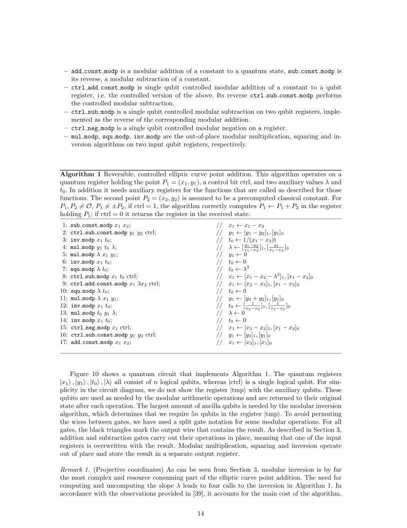
– add const modp is a modular addition of a constant to a quantum state, sub const modp isits reverse, a modular subtraction of a constant.

– ctrl add const modp is single qubit controlled modular addition of a constant to a qubitregister, i.e. the controlled version of the above. Its reverse ctrl sub const modp performsthe controlled modular subtraction.

– ctrl sub modp is a single qubit controlled modular subtraction on two qubit registers, imple-mented as the reverse of the corresponding modular addition.

– ctrl neg modp is a single qubit controlled modular negation on a register.

– mul modp, squ modp, inv modp are the out-of-place modular multiplication, squaring and in-version algorithms on two input qubit registers, respectively.

Algorithm 1 Reversible, controlled elliptic curve point addition. This algorithm operates on aquantum register holding the point P1 = (x1, y1), a control bit ctrl, and two auxiliary values λ andt0. In addition it needs auxiliary registers for the functions that are called as described for thosefunctions. The second point P2 = (x2, y2) is assumed to be a precomputed classical constant. ForP1, P2 6= O, P1 6= ±P2, if ctrl = 1, the algorithm correctly computes P1 ← P1 + P2 in the registerholding P1; if ctrl = 0 it returns the register in the received state.

1: sub const modp x1 x2;2: ctrl sub const modp y1 y2 ctrl;3: inv modp x1 t0;4: mul modp y1 t0 λ;5: mul modp λ x1 y1;6: inv modp x1 t0;7: squ modp λ t0;8: ctrl sub modp x1 t0 ctrl;9: ctrl add const modp x1 3x2 ctrl;

10: squ modp λ t0;11: mul modp λ x1 y1;12: inv modp x1 t0;13: mul modp t0 y1 λ;14: inv modp x1 t0;15: ctrl neg modp x1 ctrl;16: ctrl sub const modp y1 y2 ctrl;17: add const modp x1 x2;

// x1 ← x1 − x2// y1 ← [y1 − y2]1, [y1]0// t0 ← 1/(x1 − x2)t// λ← [ y1−y2

x1−x2]1, [

y1x1−x2

]0// y1 ← 0// t0 ← 0// t0 ← λ2

// x1 ← [x1 − x2 − λ2]1, [x1 − x2]0// x1 ← [x2 − x3]1, [x1 − x2]0// t0 ← 0// y1 ← [y3 + y2]1, [y1]0// t0 ← [ 1

x2−x3]1, [

1x1−x2

]0// λ← 0// t0 ← 0// x1 ← [x3 − x2]1, [x1 − x2]0// y1 ← [y3]1, [y1]0// x1 ← [x3]1, [x1]0

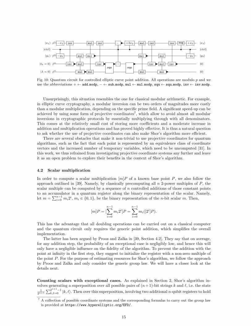
Figure 10 shows a quantum circuit that implements Algorithm 1. The quantum registers|x1〉 , |y1〉 , |t0〉 , |λ〉 all consist of n logical qubits, whereas |ctrl〉 is a single logical qubit. For sim-plicity in the circuit diagram, we do not show the register |tmp〉 with the auxiliary qubits. Thesequbits are used as needed by the modular arithmetic operations and are returned to their originalstate after each operation. The largest amount of ancilla qubits is needed by the modular inversionalgorithm, which determines that we require 5n qubits in the register |tmp〉. To avoid permutingthe wires between gates, we have used a split gate notation for some modular operations. For allgates, the black triangles mark the output wire that contains the result. As described in Section 3,addition and subtraction gates carry out their operations in place, meaning that one of the inputregisters is overwritten with the result. Modular multiplication, squaring and inversion operateout of place and store the result in a separate output register.

Remark 1. (Projective coordinates) As can be seen from Section 3, modular inversion is by farthe most complex and resource consuming part of the elliptic curve point addition. The need forcomputing and uncomputing the slope λ leads to four calls to the inversion in Algorithm 1. Inaccordance with the observations provided in [39], it accounts for the main cost of the algorithm.

14

|x1〉 /n −x2 inv mul inv − I +3x2 mul inv inv neg +x2 |x3〉

|ctrl〉 • • • • • |ctrl〉

|y1〉 /n −y2 mul mul I mul I mul −y2 |y3〉

|t0 = 0〉 /n inv I mul inv Isqu

I −squ

I inv I mul inv I |0〉

|λ = 0〉 /n mul I mul mul mul I |0〉

Fig. 10: Quantum circuit for controlled elliptic curve point addition. All operations are modulo p and weuse the abbreviations +← add modp, − ← sub modp, mul← mul modp, squ← squ modp, inv← inv modp.

Unsurprisingly, this situation resembles the one for classical modular arithmetic. For example,in elliptic curve cryptography, a modular inversion can be two orders of magnitudes more costlythan a modular multiplication, depending on the specific prime field. A significant speed-up can beachieved by using some form of projective coordinates7, which allow to avoid almost all modularinversions in cryptographic protocols by essentially multiplying through with all denominators.This comes at the relatively small cost of storing more coefficients and a moderate increase inaddition and multiplication operations and has proved highly effective. It is thus a natural questionto ask whether the use of projective coordinates can also make Shor’s algorithm more efficient.

There are several obstacles that make it non-trivial to use projective coordinates for quantumalgorithms, such as the fact that each point is represented by an equivalence class of coordinatevectors and the increased number of temporary variables, which need to be uncomputed [31]. Inthis work, we thus refrained from investigating projective coordinate systems any further and leaveit as an open problem to explore their benefits in the context of Shor’s algorithm.

4.2 Scalar multiplication

In order to compute a scalar multiplication [m]P of a known base point P , we also follow theapproach outlined in [39]. Namely, by classically precomputing all n 2-power multiples of P , thescalar multiple can be computed by a sequence of n controlled additions of those constant pointsto an accumulator in a quantum register along the binary representation of the scalar. Namely,let m =

∑n−1i=0 mi2

i, mi ∈ {0, 1}, be the binary representation of the n-bit scalar m. Then,

[m]P = [

n−1∑i=0

mi2i]P =

n−1∑i=0

mi([2i]P ).

This has the advantage that all doubling operations can be carried out on a classical computerand the quantum circuit only requires the generic point addition, which simplifies the overallimplementation.

The latter has been argued by Proos and Zalka in [39, Section 4.2]. They say that on average,for any addition step, the probability of an exceptional case is negligibly low, and hence this willonly have a negligible influence on the fidelity of the algorithm. To prevent the addition with thepoint at infinity in the first step, they suggest to initialize the register with a non-zero multiple ofthe point P . For the purpose of estimating resources for Shor’s algorithm, we follow the approachby Proos and Zalka and only consider the generic group law. We will have a closer look at thedetails next.

Counting scalars with exceptional cases. As explained in Section 2, Shor’s algorithm in-volves generating a superposition over all possible pairs of (n+ 1)-bit strings k and `, i.e. the state

12n+1

∑2n+1−1k,`=0 |k, `〉. Then over this superposition, involving two additional n-qubit registers to hold

7 A collection of possible coordinate systems and the corresponding formulas to carry out the group lawis provided at https://www.hyperelliptic.org/EFD/.

15

an elliptic curve point, one computes a double scalar multiplication 12n+1

∑2n+1−1k,`=0 |k, `〉 |[k]P + [`]Q〉

of the input points given by the ECDLP instance.

Figure 1 depicts the additional elliptic curve point register to be initialized with a representationof the neutral element O. But if we only consider the generic case of the group law, the firstaddition of P would already involve an exceptional case due to one of the inputs being O. Proosand Zalka [39] propose to solve this issue by instead initializing the register with a uniform randomnon-zero multiple of P , say [a]P for a random a ∈ {1, 2, . . . , r− 1}. Recall that r is the order of Pwhich we assume to be a large prime. Now, if a /∈ {1, r− 1}, the first point addition with P worksas a generic point addition. With high probability, this solves the issue of an exception in the firstaddition, but still exceptions occur along the way for many of the possibilities for bit strings kand `. Whenever a bit string leads to an exceptional case in the group law, it produces a wrongresult for the double scalar multiplication and pollutes the quantum register. We call such a scalarinvalid. For Shor’s algorithm to work, the overall number of such invalid scalars must be smallenough. In the following we count these scalars, similar to the reasoning in [39].

Exceptional additions of a point to itself. Let a ∈ {1, 2, . . . , r − 1} be fixed and writek =

∑ni=0 ki2

i, ki ∈ {0, 1}. We first consider the exceptional case in which both input points arethe same, which we call an exceptional doubling. If a = 1, this occurs in the first iteration fork0 = 1, because we attempt to add P to itself. This means that for a = 1, all scalars k with k0 = 1lead to a wrong result and therefore half of the scalars are invalid, i.e. in total 2n.

For a = 2, the case k0 = 1 is not a problem since the addition [2]P + P is a generic addition,but (k0, k1) = (0, 1) leads to an exceptional doubling operation in the second controlled addition.This means that all scalars (0, 1, k2, . . . , kn) are invalid. These are one quarter of all scalars, i.e.2n−1.

For general a, assume that k is a scalar such that the first i − 1 additions, i ∈ {1, . . . , n},controlled on the bits k0, . . . , ki−1 do not encounter any exceptional doubling cases. The i-thaddition means the addition of [2i]P for 0 ≤ i ≤ n. Then the i-th addition is an exceptionaldoubling if, and only if

a+ (k0 + k1 · 2 + · · ·+ ki−1 · 2i−1) = 2i (mod r).

If i is such that 2i < r. Then, the above condition is equivalent to the condition a = 2i−∑i−1j=0 kj ·2j

over the integers. This means that an a can only lead to an exceptional doubling in the i-th additionif a ∈ {1, . . . , 2i}. Furthermore, if i is the smallest integer, such that there exist k0, . . . , ki−1 suchthat this equation holds, we can conclude that a ∈ {2i−1 + 1, . . . , 2i} and ki−1 = 0. In that case,any scalar of the form (k0, . . . , ki−2, 0, 1, ∗, . . . , ∗) is invalid. The number of such scalars is 2n−i.

If i is instead such that 2i ≥ r and if a ≤ 2i − µr for some positive integer µ ≤ b2i/rc, then inaddition to the solutions given by the equation over the integers as above, there exist additionalsolutions given by the condition a = (2i − µr) −

∑i−1j=0 kj · 2j , namely (k0, . . . , ki−1, 1, ∗, . . . , ∗).

The maximal number of such scalars is b(2i−a)/rc2n−i, but we might have counted some of thesealready.

For a given a ∈ {1, 2, . . . , r − 1}, denote by Sa the set of scalars that contain an exceptionaldoubling, i.e. the set of all k = (k0, k1, . . . , kn) ∈ {0, 1, }n+1 such that there occurs an exceptional

doubling when executing the addition [a +∑i−1j=0 kj · 2j ]P + [2i]P for any i ∈ {0, 1, . . . , n}. Let

ia = dlog(a)e. Then, an upper bound for the number of invalid scalars is given by

#Sa ≤ 2n−ia +

n∑i=dlog(r)e

b(2i − a)/rc2n−i.

Hasse’s bound gives dlog(r)e ≥ n− 1, which means that

#Sa ≤ 2n−ia + 2b(2n−1 − a)/rc+ b(2n − a)/rc ≤ 2n−ia + 8.

16

Hence on average, the number of invalid scalars over a uniform choice of k ∈ {1, . . . , r− 1} can bebounded as

r−1∑a=1

Pr(a) ·#Sa ≤1

r − 1

r−1∑a=1

2n−dlog(a)e + 8.

Grouping values of a with the same dlog(a)e and possibly adding terms at the end of the sum, thefirst term can be simplified and further bounded by 1

r−1 (2n + dlog(r − 1)e2n−1) = (2 + dlog(r −1)e) 2n−1

r−1 . For large enough bitsizes, we use that r − 1 ≥ 2n−1 and obtain the upper bound onthe expected number of invalid scalars of roughly dlog(r)e + 10 ≈ n + 10. This corresponds to anegligible fraction of about n/2n+1 of all scalars.

Exceptional additions of a point to its negative. To determine the number of invalid scalarsarising from the second possibility of exceptions, namely the addition of a point to its negative, wecarry out the same arguments. An invalid scalar is a scalar that leads to an addition [−2i]P+[2i]P .The condition on the scalar a is slightly changed with 2i replaced by r − 2i, i.e.

a+ (k0 + k1 · 2 + · · ·+ ki−1 · 2i−1) = r − 2i (mod r).

Whenever this equation holds over the integers, i.e. r − a = 2i + (k0 + k1 · 2 + · · · + ki−1 · 2i−1)holds, we argue analogously as above. If 2i < r and r − a ∈ {2i, . . . , 2i+1 − 1}, there are 2n−i

invalid scalars. Similar arguments as above for the steps such that 2i > r lead to similar counts.Overall, we conclude that in this case the fraction of invalid scalars can also be approximated byn/2n+1.

Exceptional additions of the point at infinity. Since the quantum register holding the ellip-tic curve point is initialized with a non-zero point and the multiples of P added during the scalarmultiplication are also non-zero, the point at infinity can only occur as the result of an exceptionaladdition of a point to its negative. Therefore, all scalars for which this occurs have been excludedpreviously and we do not further consider this case.

Overall, an approximate upper bound for the fraction of invalid scalars among the superpositionof all scalars due to exceptional cases in the addition law is 2n/2n+1 = n/2n.

Double scalar multiplication. In Shor’s algorithm with the above modification, one needs tocompute a double scalar multiplication [a+ k]P + [`]Q where P and Q are the points given by theECDLP instance we are trying to solve and a is a fixed uniformly random non-zero integer modulor. We are trying to find the integer m modulo r such that Q = [m]P . Since r is a large prime, wecan assume that m ∈ {1, . . . , r− 1} and we can write P = [m−1]Q. Multiplication by m−1 on theelements modulo r is a bijection, simply permuting these scalars. Hence, after having dealt withthe scalar multiplication to compute [a+ k]P above, we can now apply the same treatment to thesecond part, the addition of [`]Q to this result.

Let a be chosen uniformly at random. For any k, we write [a+ k]P = [m−1(a+ k)]Q. Assumethat k is a valid scalar for this fixed choice of a. Then, the computation of [a+k]P did not involveany exceptional cases and thus [a+ k]P 6= O, which means that a+ k 6= 0 (mod r). If we assumethat the unknown discrete logarithm m has been chosen from {1, . . . , r− 1} uniformly at random,then the value b = m−1(a+k) mod r is uniform random in {1, . . . , r−1} as well, and we have thesame situation as above when we were looking at the choice of a and the computation of [a+ k]P .

Using the rough upper bound for the fraction of invalid scalars from above, for a fixed randomchoice of a, the probability that a random scalar k is valid, is at least 1 − n/2n. Further, theprobability that (k, `) is a pair of valid scalars for computing [a + k]P + [`]Q, conditioned on kbeing valid for computing [a+ k]P is also at least 1− n/2n. Hence, for a fixed uniform random a,the probability for (k, `) being valid is at least (1− n/2n)2 = 1− n/2n−1 + n2/22n ≈ 1− n/2n−1.This result confirms the rough estimate by Proos and Zalka [39, Section 4.2] of a fidelity loss of4n/p ≥ 4n/2n+1.

17

Remark 2. (Complete addition formulas) There exist complete formulas for the group law on anelliptic curve in Weierstrass form [7]. This means that there is a single formula that can evaluatethe group law on any pair of Fp-rational points on the curve and thus avoids the occurrence ofexceptional cases altogether. For classical computations, this comes at the cost of a relativelysmall slowdown [40]. Using such formulas would increase the algorithm’s fidelity in comparisonto the above method. Furthermore, there exist alternative curve models for elliptic curves whichallow coordinate systems that offer even more efficient complete formulas. One such example isthe twisted Edwards form of an elliptic curve [4]. However, not all elliptic curves allow a curvemodel in twisted Edwards form, like, for example, the prime order NIST curves. We leave it as anopen problem to investigate the use of a complete group law, or more generally the use of differentcurve models and coordinate systems in Shor’s ECDLP algorithm.

5 Cost and resource estimates for Shor’s algorithm

We implemented the reversible algorithm for elliptic curve point addition on elliptic curves E inshort Weierstrass form defined over a prime field Fp, where p has n bits, as shown in Algorithm 1and Figure 10 in Section 4 in F# within the quantum computing software tool suite LIQUi|〉[52]. This allows us to test and simulate the circuit and all its components and obtain precisecounts of the number of qubits, the number of Toffoli gates and the Toffoli gate depth for aworking simulation. We thus do not have to rely on mere estimates obtained by pen-and-papercalculations and thus gain a higher confidence in the results. When implementing the algorithms,our overall emphasis was to minimize first the number of required logical qubits and second theToffoli gate count.

We have simulated and tested our implementation for cryptographically relevant parametersizes and were able to simulate the elliptic curve point addition circuit for curves over prime fieldsof size up to 521 bits. For each case, we computed the number of qubits required to implementthe circuit, and its size and depth in terms of Toffoli gates.

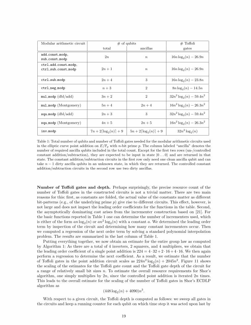
Number of logical qubits. The number of logical qubits of the modular arithmetic circuits inour simulation that are needed in the elliptic curve point addition are given in Table 1. We listeach function with its total required number of qubits and the number of ancilla qubits includedin that number. All ancilla qubits are expected to be input in the state |0〉 and are returned inthat state, except for the circuits in the first two rows, which only require one or two such ancillaqubits and n−1 or n−2 ancillas in an unknown state to which they will be returned. The addition,subtraction and negation circuits all work in place, such that one n-qubit input register is replacedwith the result. The multiplication, squaring and inversion circuits require an n-qubit register withwhich the result of the computation is XOR-ed.

Although the modular multiplication circuit based on modular doubling and additions usesless qubits than Montgomery multiplication, we have used the Montgomery approach to reportthe results of our experiments. Since the lower bound on the overall required number of qubitsis dictated by the modular inversion circuit, neither multiplication approach adds qubit registersto the elliptic curve addition circuit since they can use ancilla qubits provided by the inversionalgorithm. We therefore find that the Montgomery circuit is the better choice then because itreduces the number of Toffoli gates substantially.

Because the maximum amount of qubits is used during an inversion operation, the overallnumber of logical qubits for the controlled elliptic curve point addition in our simulation is

9n+ 2dlog2(n)e+ 10.

In addition to the 7n+ 2dlog2(n)e+ 9 required by the inversion, an additional qubit is needed forthe control qubit |ctrl〉 of the overall operation and 2n more qubits are needed since two n-qubitregisters need to hold intermediate results during each inversion.

18

Modular arithmetic circuit # of qubits # Toffoli

total ancillas gates

add const modp,sub const modp

2n n 16n log2(n)− 26.9n

ctrl add const modp,ctrl sub const modp 2n+ 1 n 16n log2(n)− 26.9n

ctrl sub modp 2n+ 4 3 16n log2(n)− 23.8n

ctrl neg modp n+ 3 2 8n log2(n)− 14.5n

mul modp (dbl/add) 3n+ 2 2 32n2 log2(n)− 59.4n2

mul modp (Montgomery) 5n+ 4 2n+ 4 16n2 log2(n)− 26.3n2

squ modp (dbl/add) 2n+ 3 3 32n2 log2(n)− 59.4n2

squ modp (Montgomery) 4n+ 5 2n+ 5 16n2 log2(n)− 26.3n2

inv modp 7n+ 2dlog2(n)e+ 9 5n+ 2dlog2(n)e+ 9 32n2 log2(n)

Table 1: Total number of qubits and number of Toffoli gates needed for the modular arithmetic circuits usedin the elliptic curve point addition on E/Fp with n-bit prime p. The column labeled “ancilla” denotes thenumber of required ancilla qubits included in the total count. Except for the first two rows (un-/controlledconstant addition/subtraction), they are expected to be input in state |0 . . . 0〉 and are returned in thatstate. The constant addition/subtraction circuits in the first row only need one clean ancilla qubit and cantake n− 1 dirty ancilla qubits in an unknown state, in which they are returned. The controlled constantaddition/subtraction circuits in the second row use two dirty ancillas.

Number of Toffoli gates and depth. Perhaps surprisingly, the precise resource count of thenumber of Toffoli gates in the constructed circuits is not a trivial matter. There are two mainreasons for this: first, as constants are folded, the actual value of the constants matter as differentbit-patterns (e.g., of the underlying prime p) give rise to different circuits. This effect, however, isnot large and does not impact the leading order coefficients for the functions in the table. Second,the asymptotically dominating cost arises from the incrementer construction based on [21]. Forthe basic functions reported in Table 1 one can determine the number of incrementers used, whichis either of the form an log2(n) or an2 log2(n) with a constant a. We determined the leading orderterm by inspection of the circuit and determining how many constant incrementers occur. Thenwe computed a regression of the next order term by solving a standard polynomial interpolationproblem. The results are summarized in the last column of Table 1.

Putting everything together, we now obtain an estimate for the entire group law as computedby Algorithm 1: As there are a total of 4 inverters, 2 squarers, and 4 multipliers, we obtain thatthe leading order coefficient of a single point addition is 224 = 4 ·32 + 2 ·16 + 4 ·16. We then againperform a regression to determine the next coefficient. As a result, we estimate that the numberof Toffoli gates in the point addition circuit scales as 224n2 log2(n) + 2045n2. Figure 11 showsthe scaling of the estimates for the Toffoli gate count and the Toffoli gate depth of the circuit fora range of relatively small bit sizes n. To estimate the overall resource requirements for Shor’salgorithm, one simply multiplies by 2n, since the controlled point addition is iterated 2n times.This leads to the overall estimate for the scaling of the number of Toffoli gates in Shor’s ECDLPalgorithm as

(448 log2(n) + 4090)n3.

With respect to a given circuit, the Toffoli depth is computed as follows: we sweep all gates inthe circuits and keep a running counter for each qubit on which time step it was acted upon last by

19

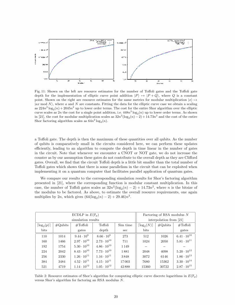
Fig. 11: Shown on the left are resource estimates for the number of Toffoli gates and the Toffoli gatedepth for the implementation of elliptic curve point addition |P 〉 7→ |P +Q〉, where Q is a constantpoint. Shown on the right are resource estimates for the same metrics for modular multiplication |x〉 7→|ax mod N〉, where a and N are constants. Fitting the data for the elliptic curve case we obtain a scalingas 224n2 log2(n) + 2045n2 up to lower order terms. The cost for the entire Shor algorithm over the ellipticcurve scales as 2n the cost for a single point addition, i.e. 448n3 log2(n) up to lower order terms. As shownin [21], the cost for modular multiplication scales as 32n2(log2(n)− 2) + 14.73n2 and the cost of the entireShor factoring algorithm scales as 64n2 log2(n).

a Toffoli gate. The depth is then the maximum of these quantities over all qubits. As the numberof qubits is comparatively small in the circuits considered here, we can perform these updatesefficiently, leading to an algorithm to compute the depth in time linear in the number of gatesin the circuit. Note that whenever we encounter a CNOT or NOT gate, we do not increase thecounter as by our assumption these gates do not contribute to the overall depth as they are Cliffordgates. Overall, we find that the circuit Toffoli depth is a little bit smaller than the total number ofToffoli gates which shows that there is some parallelism in the circuit that can be exploited whenimplementing it on a quantum computer that facilitates parallel application of quantum gates.

We compare our results to the corresponding simulation results for Shor’s factoring algorithmpresented in [21], where the corresponding function is modular constant multiplication. In thiscase, the number of Toffoli gates scales as 32n2(log2(n) − 2) + 14.73n2, where n is the bitsize ofthe modulus to be factored. As above, to estimate the overall resource requirements, one againmultiplies by 2n, which gives (64(log2(n)− 2) + 29.46)n3.

ECDLP in E(Fp) Factoring of RSA modulus N

simulation results interpolation from [21]

dlog2(p)e #Qubits #Toffoli Toffoli Sim time dlog2(N)e #Qubits #Toffoli

bits gates depth sec bits gates

110 1014 9.44 · 109 8.66 · 109 273 512 1026 6.41 · 1010

160 1466 2.97 · 1010 2.73 · 1010 711 1024 2050 5.81 · 1011

192 1754 5.30 · 1010 4.86 · 1010 1 149 − − −224 2042 8.43 · 1010 7.73 · 1010 1 881 2048 4098 5.20 · 1012

256 2330 1.26 · 1011 1.16 · 1011 3 848 3072 6146 1.86 · 1013

384 3484 4.52 · 1011 4.15 · 1011 17 003 7680 15362 3.30 · 1014

521 4719 1.14 · 1012 1.05 · 1012 42 888 15360 30722 2.87 · 1015

Table 2: Resource estimates of Shor’s algorithm for computing elliptic curve discrete logarithms in E(Fp)versus Shor’s algorithm for factoring an RSA modulus N .

20

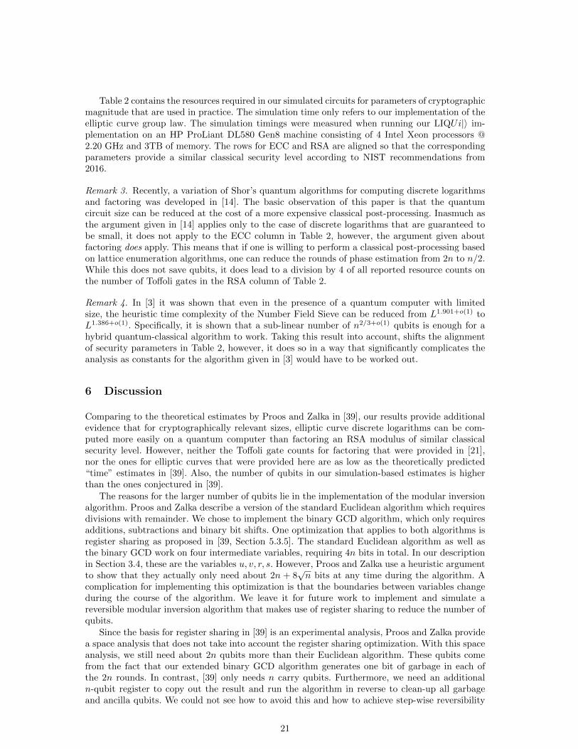
Table 2 contains the resources required in our simulated circuits for parameters of cryptographicmagnitude that are used in practice. The simulation time only refers to our implementation of theelliptic curve group law. The simulation timings were measured when running our LIQUi|〉 im-plementation on an HP ProLiant DL580 Gen8 machine consisting of 4 Intel Xeon processors @2.20 GHz and 3TB of memory. The rows for ECC and RSA are aligned so that the correspondingparameters provide a similar classical security level according to NIST recommendations from2016.

Remark 3. Recently, a variation of Shor’s quantum algorithms for computing discrete logarithmsand factoring was developed in [14]. The basic observation of this paper is that the quantumcircuit size can be reduced at the cost of a more expensive classical post-processing. Inasmuch asthe argument given in [14] applies only to the case of discrete logarithms that are guaranteed tobe small, it does not apply to the ECC column in Table 2, however, the argument given aboutfactoring does apply. This means that if one is willing to perform a classical post-processing basedon lattice enumeration algorithms, one can reduce the rounds of phase estimation from 2n to n/2.While this does not save qubits, it does lead to a division by 4 of all reported resource counts onthe number of Toffoli gates in the RSA column of Table 2.

Remark 4. In [3] it was shown that even in the presence of a quantum computer with limitedsize, the heuristic time complexity of the Number Field Sieve can be reduced from L1.901+o(1) toL1.386+o(1). Specifically, it is shown that a sub-linear number of n2/3+o(1) qubits is enough for ahybrid quantum-classical algorithm to work. Taking this result into account, shifts the alignmentof security parameters in Table 2, however, it does so in a way that significantly complicates theanalysis as constants for the algorithm given in [3] would have to be worked out.

6 Discussion

Comparing to the theoretical estimates by Proos and Zalka in [39], our results provide additionalevidence that for cryptographically relevant sizes, elliptic curve discrete logarithms can be com-puted more easily on a quantum computer than factoring an RSA modulus of similar classicalsecurity level. However, neither the Toffoli gate counts for factoring that were provided in [21],nor the ones for elliptic curves that were provided here are as low as the theoretically predicted“time” estimates in [39]. Also, the number of qubits in our simulation-based estimates is higherthan the ones conjectured in [39].

The reasons for the larger number of qubits lie in the implementation of the modular inversionalgorithm. Proos and Zalka describe a version of the standard Euclidean algorithm which requiresdivisions with remainder. We chose to implement the binary GCD algorithm, which only requiresadditions, subtractions and binary bit shifts. One optimization that applies to both algorithms isregister sharing as proposed in [39, Section 5.3.5]. The standard Euclidean algorithm as well asthe binary GCD work on four intermediate variables, requiring 4n bits in total. In our descriptionin Section 3.4, these are the variables u, v, r, s. However, Proos and Zalka use a heuristic argumentto show that they actually only need about 2n + 8

√n bits at any time during the algorithm. A

complication for implementing this optimization is that the boundaries between variables changeduring the course of the algorithm. We leave it for future work to implement and simulate areversible modular inversion algorithm that makes use of register sharing to reduce the number ofqubits.

Since the basis for register sharing in [39] is an experimental analysis, Proos and Zalka providea space analysis that does not take into account the register sharing optimization. With this spaceanalysis, we still need about 2n qubits more than their Euclidean algorithm. These qubits comefrom the fact that our extended binary GCD algorithm generates one bit of garbage in each ofthe 2n rounds. In contrast, [39] only needs n carry qubits. Furthermore, we need an additionaln-qubit register to copy out the result and run the algorithm in reverse to clean-up all garbageand ancilla qubits. We could not see how to avoid this and how to achieve step-wise reversibility

21

for the extended binary Euclidean algorithm. We leave it as a future challenge to match or evenlower the number of qubits for reversible modular inversion from [39].

To summarize, we presented quantum circuits to implement Shor’s algorithm to solve theECDLP. We analyzed the resources required to implement these circuits and simulated large partsof them on a classical machine. Indeed, the overwhelming majority of gates in our circuits areToffoli, CNOT, and NOT gates, which implement the controlled addition of an elliptic curve pointthat is known at circuit generation time. We were able to classically simulate the point additioncircuit and hence test it for implementation bugs. Our findings imply that attacking elliptic curvecryptography is indeed easier than attacking RSA, even for relatively small key sizes.

Acknowledgments. We thank Christof Zalka for feedback and discussions and the anonymousreviewers for their valuable comments.

References

1. Matthew Amy, Dmitri Maslov, Michele Mosca, and Martin Roetteler. A meet-in-the-middle algorithmfor fast synthesis of depth-optimal quantum circuits. Computer-Aided Design of Integrated Circuitsand Systems, IEEE Transactions on, 32(6):818–830, June 2013.

2. Stephane Beauregard. Circuit for Shor’s algorithm using 2n+3 qubits. Quantum Info. Comput.,3(2):175–185, March 2003.

3. Daniel J. Bernstein, Jean-Francois Biasse, and Michele Mosca. A low-resource quantum factoringalgorithm. In Lange and Takagi [28], pages 330–346.

4. Daniel J. Bernstein, Peter Birkner, Marc Joye, Tanja Lange, and Christiane Peters. Twisted Edwardscurves. In Serge Vaudenay, editor, Progress in Cryptology - AFRICACRYPT 2008, First InternationalConference on Cryptology in Africa, Casablanca, Morocco, June 11-14, 2008. Proceedings, volume 5023of Lecture Notes in Computer Science, pages 389–405. Springer, 2008.

5. Simon Blake-Wilson, Nelson Bolyard, Vipul Gupta, Chris Hawk, and Bodo Moeller. Elliptic curvecryptography (ECC) cipher suites for Transport Layer Security (TLS). RFC 4492, 2006.

6. Joppe W. Bos, Craig Costello, and Andrea Miele. Elliptic and hyperelliptic curves: A practicalsecurity analysis. In Hugo Krawczyk, editor, Public-Key Cryptography - PKC 2014 - 17th InternationalConference on Practice and Theory in Public-Key Cryptography, Buenos Aires, Argentina, March 26-28, 2014. Proceedings, volume 8383 of Lecture Notes in Computer Science, pages 203–220. Springer,2014.

7. Wieb Bosma and Hendrik W. Lenstra. Complete system of two addition laws for elliptic curves.Journal of Number Theory, 53(2):229–240, 1995.

8. Certicom Research. Standards for efficient cryptography 2: Recommended elliptic curve domain pa-rameters. Standard SEC2, Certicom, 2000.

9. Richard Crandall and Carl Pomerance, editors. Prime Numbers - A Computational Perspective.Springer, 2005.

10. Tim Dierks and Eric Rescorla. The Transport Layer Security (TLS) protocol version 1.2. RFC 5246,2008.

11. Whitfield Diffie and Martin E. Hellman. New directions in cryptography. IEEE Trans. InformationTheory, 22(6):644–654, 1976.

12. Roger Dingledine, Nick Mathewson, and Paul F. Syverson. Tor: The second-generation onion router.In Matt Blaze, editor, Proceedings of the 13th USENIX Security Symposium, August 9-13, 2004, SanDiego, CA, USA, pages 303–320. USENIX, 2004.

13. ECC Brainpool. ECC Brainpool Standard Curves and Curve Generation. http://www.

ecc-brainpool.org/download/Domain-parameters.pdf, 2005.14. Martin Ekera and Johan Hastad. Quantum algorithms for computing short discrete logarithms and

factoring RSA integers. In Lange and Takagi [28], pages 347–363.15. Austin G. Fowler, Matteo Mariantoni, John M. Martinis, and Andrew N. Cleland. Surface codes:

Towards practical large-scale quantum computation. Phys. Rev. A, 86:032324, 2012. arXiv:1208.0928.16. Steven D. Galbraith and Pierrick Gaudry. Recent progress on the elliptic curve discrete logarithm

problem. Des. Codes Cryptography, 78(1):51–72, 2016.17. Taher El Gamal. A public key cryptosystem and a signature scheme based on discrete logarithms.

In G. R. Blakley and David Chaum, editors, Advances in Cryptology, Proceedings of CRYPTO ’84,Santa Barbara, California, USA, August 19-22, 1984, Proceedings, volume 196 of Lecture Notes inComputer Science, pages 10–18. Springer, 1984.

22

18. Daniel M. Gordon. Discrete logarithms in GF(P) using the number field sieve. SIAM J. DiscreteMath., 6(1):124–138, 1993.

19. Robert Griffiths and Chi-Sheng Niu. Semiclassical Fourier transform for quantum computation. Phys.Rev. Letters, 76(17):3228–3231, 1996.

20. Mike Hamburg. Ed448-Goldilocks, a new elliptic curve. IACR Cryptology ePrint Archive, 2015:625,2015.

21. Thomas Haner, Martin Roetteler, and Krysta M. Svore. Factoring using 2n+2 qubits with Toffolibased modular multiplication. 2016. arXiv preprint arXiv:1611.07995.

22. Arno Hollosi, Gregor Karlinger, Thomas Rossler, Martin Centner, et al. Die osterreichischeBurgerkarte. http://www.buergerkarte.at/konzept/securitylayer/spezifikation/20080220/,2008.

23. Don Johnson, Alfred Menezes, and Scott A. Vanstone. The elliptic curve digital signature algorithm(ECDSA). Int. J. Inf. Sec., 1(1):36–63, 2001.

24. Antoine Joux and Reynald Lercier. Improvements to the general number field sieve for discrete loga-rithms in prime fields. A comparison with the gaussian integer method. Math. Comput., 72(242):953–967, 2003.

25. Burton S. Kaliski Jr. The Montgomery inverse and its applications. IEEE Trans. Computers,44(8):1064–1065, 1995.

26. Vadym Kliuchnikov, Dmitri Maslov, and Michele Mosca. Practical approximation of single-qubit uni-taries by single-qubit quantum Clifford and T circuits. IEEE Transactions on Computers, 65(1):161–172, 2016.

27. Neal Koblitz. Elliptic curve cryptosystems. Mathematics of Computation, 48(177):203–209, 1987.28. Tanja Lange and Tsuyoshi Takagi, editors. Post-Quantum Cryptography - 8th International Workshop,

PQCrypto 2017, Utrecht, The Netherlands, June 26-28, 2017, Proceedings, volume 10346 of LectureNotes in Computer Science. Springer, 2017.

29. Adam Langley, Mike Hamburg, and Sean Turner. Elliptic curves for security. RFC 7748, 2016.30. Arjen K. Lenstra and Hendrik W. Lenstra, editors. The development of the number field sieve, volume

1554 of Lecture Notes in Mathematics. Springer, 1993.

31. Dmitri Maslov, Jimson Mathew, Donny Cheung, and Dhiraj K. Pradhan. An O(m2)-depth quantumalgorithm for the elliptic curve discrete logarithm problem over GF(2m). Quantum Information &Computation, 9(7):610–621, 2009.

32. Victor S. Miller. Use of elliptic curves in cryptography. In Hugh C. Williams, editor, Advances inCryptology - CRYPTO ’85, Santa Barbara, California, USA, August 18-22, 1985, Proceedings, volume218 of Lecture Notes in Computer Science, pages 417–426. Springer, 1985.

33. Peter L. Montgomery. Modular multiplication without trial division. Mathematics of Computation,44(170):519–521, 1985.

34. Satoshi Nakamoto. Bitcoin: A peer-to-peer electronic cash system. http://bitcoin.org/bitcoin.

pdf, 2009.35. Michael. A. Nielsen and Ike. L. Chuang. Quantum Computation and Quantum Information. Cambridge

University Press, Cambridge, UK, 2000.36. Kenneth G. Paterson. Formal request from TLS WG to CFRG for new elliptic curves. CFRG mailing

list, 2014-07-14, http://www.ietf.org/mail-archive/web/cfrg/current/msg04655.html.37. John M. Pollard. Monte Carlo methods for index computation mod p. Math. Comput., 32(143):918–

924, 1978.38. John M. Pollard. Kangaroos, Monopoly and discrete logarithms. J. Cryptology, 13(4):437–447, 2000.39. John Proos and Christof Zalka. Shor’s discrete logarithm quantum algorithm for elliptic curves.

Quantum Information & Computation, 3(4):317–344, 2003.40. Joost Renes, Craig Costello, and Lejla Batina. Complete addition formulas for prime order elliptic

curves. In Marc Fischlin and Jean-Sebastien Coron, editors, Advances in Cryptology - EUROCRYPT2016 - 35th Annual International Conference on the Theory and Applications of Cryptographic Tech-niques, Vienna, Austria, May 8-12, 2016, Proceedings, Part I, volume 9665 of Lecture Notes in Com-puter Science, pages 403–428. Springer, 2016.

41. Ronald L. Rivest, Adi Shamir, and Leonard M. Adleman. A method for obtaining digital signaturesand public-key cryptosystems. Commun. ACM, 21(2):120–126, 1978.

42. Peter Selinger. Quantum circuits of T -depth one. Phys. Rev. A, 87:042302, 2013.43. Peter Selinger. Efficient Clifford+T approximation of single-qubit operators. Quantum Information

& Computation, 15(1-2):159–180, 2015.44. Peter W. Shor. Algorithms for quantum computation: Discrete logarithms and factoring. In 35th An-

nual Symposium on Foundations of Computer Science, Santa Fe, New Mexico, USA, 20-22 November1994, pages 124–134. IEEE Computer Society, 1994.

23

45. Peter W. Shor. Polynomial-time algorithms for prime factorization and discrete logarithms on aquantum computer. SIAM J. Comput., 26(5):1484–1509, October 1997.

46. Joseph H. Silverman. The Arithmetic of Elliptic Curves (2nd Edition). Number 106 in Graduate textsin mathematics. Springer-Verlag, 2009.

47. Douglas Stebila and Jon Green. Elliptic curve algorithm integration in the Secure Shell TransportLayer. RFC 5656, 2009.

48. Josef Stein. Journal of Computational Physics, 1(3):397–405, 1967.49. Yasuhiro Takahashi, Seiichiro Tani, and Noboru Kunihiro. Quantum addition circuits and unbounded

fan-out. Quantum Information & Computation, 10(9&10):872–890, 2010.50. U.S. Department of Commerce/National Institute of Standards and Technology. Digital Signature

Standard (DSS). FIPS-186-4, 2013. http://nvlpubs.nist.gov/nistpubs/FIPS/NIST.FIPS.186-4.

pdf.51. Paul C. van Oorschot and Michael J. Wiener. Parallel collision search with cryptanalytic applications.

J. Cryptology, 12(1):1–28, 1999.52. Dave Wecker and Krysta M. Svore. LIQUi|〉: A Software Design Architecture and Domain-Specific

Language for Quantum Computing, 2014. https://arxiv.org/abs/1402.4467.53. WhatsApp Inc. Whatsapp encryption overview. Technical white paper, 2016.54. Moti Yung, Yevgeniy Dodis, Aggelos Kiayias, and Tal Malkin, editors. Public Key Cryptography -

PKC 2006, 9th International Conference on Theory and Practice of Public-Key Cryptography, NewYork, NY, USA, April 24-26, 2006, Proceedings, volume 3958 of Lecture Notes in Computer Science.Springer, 2006.

24