
Method? Monte Carlo Methods Two basic principles Monte Carlo

Quantum Monte-Carlo Studies ofGeneralized Many-body Systems
by
Jørgen Høgberget
THESISfor the degree of
MASTER OF SCIENCE
(Master in Computational Physics)
Faculty of Mathematics and Natural SciencesDepartment of Physics
University of Oslo
June 2013

2
Preface
During my stay at junior high school, I had no personal interest in mathematics. When the final year wasfinished, I sought an education within the first love of my life: Music. However, sadly, my applicationwas turned down, forcing me to fall back on general topics. This is where I had my first encounter withphysics, which should turn out not to be the last.
When high school ended, I applied for an education within structural engineering at the NorwegianUniversity of Science and Technology, however, again I was turned down. Second on the list was thephysics, meteorology and astronomy program at the University of Oslo. Never in my life have I beenmore grateful for being turned down, as starting at the University of Oslo introduced me to the secondlove of my life: Programming.
During the third year of my Bachelor I had a hard time figuring out which courses I should pick. Quiterandomly, I attended a course on computational physics lectured by Morten Hjorth-Jensen. It immedi-ately hit me that he had a genuine interest in the well-being of his students. It did not take long beforeI decided to apply for a Master’s degree within the field of computational physics.
To summarize, me being here today writing this thesis is a result of extremely random events. However,I could not have landed in a better place, and I am forever grateful for my time here at the University ofOslo. So grateful in fact, that I am continuing my stay as a PhD student within the field of multi-scalephysics.
I would like to thank my fellow Master students Sarah Reimann, Sigve Bøe Skattum, and Karl Leikangerfor much appreciated help and good discussions. Sigve helped me with the minimization algorithm, thatis, the darkest chapter of this thesis. A huge thanks to Karl for all those late nights where you gave mea ride home. Finally, thank you Sarah for withstanding my horrible German phrases all these years.
My supervisor, Morten Hjorth-Jensen, deserves a special thanks for believing in me, and filling me withconfidence when it was much needed. This man is awesome.
Additionally I would like to thank the rest of the people at the computational physics research group,especially Mathilde N. Kamperud and Veronica K. B. Olsen whom with I shared my office, Svenn-ArneDragly for helping me with numerous Linux-related issues, and “brochan” Milad H. Mobarhan for all thepleasant hours spent at Nydalen Kebab. You all contribute to making this place the best it can possiblybe. Thank you!
Jørgen Høgberget
Oslo, June 2013
3

4
Contents
1 Introduction 11
I Theory 13
2 Scientific Programming 15
2.1 Programming Languages . . . . . . . . . . . . . . . . . . . . . . . . . . . . . . . . . . . . . 15
2.1.1 High-level Languages . . . . . . . . . . . . . . . . . . . . . . . . . . . . . . . . . . . 15
2.1.2 Low-level Languages . . . . . . . . . . . . . . . . . . . . . . . . . . . . . . . . . . . 16
2.2 Object Orientation . . . . . . . . . . . . . . . . . . . . . . . . . . . . . . . . . . . . . . . . 17
2.2.1 A Brief Introduction to Essential Concepts . . . . . . . . . . . . . . . . . . . . . . 18
2.2.2 Inheritance . . . . . . . . . . . . . . . . . . . . . . . . . . . . . . . . . . . . . . . . 18
2.2.3 Pointers, Typecasting and Virtual Functions . . . . . . . . . . . . . . . . . . . . . 21
2.2.4 Polymorphism . . . . . . . . . . . . . . . . . . . . . . . . . . . . . . . . . . . . . . 22
2.2.5 Const Correctness . . . . . . . . . . . . . . . . . . . . . . . . . . . . . . . . . . . . 24
2.2.6 Accessibility levels and Friend classes . . . . . . . . . . . . . . . . . . . . . . . . . 24
2.2.7 Example: PotionGame . . . . . . . . . . . . . . . . . . . . . . . . . . . . . . . . . . 25
2.3 Structuring the code . . . . . . . . . . . . . . . . . . . . . . . . . . . . . . . . . . . . . . . 29
2.3.1 File Structures . . . . . . . . . . . . . . . . . . . . . . . . . . . . . . . . . . . . . . 29
2.3.2 Class Structures . . . . . . . . . . . . . . . . . . . . . . . . . . . . . . . . . . . . . 29
3 Quantum Monte-Carlo 31
5
6 CONTENTS
3.1 Modelling Diffusion . . . . . . . . . . . . . . . . . . . . . . . . . . . . . . . . . . . . . . . . 31
3.1.1 Stating the Schrodinger Equation as a Diffusion Problem . . . . . . . . . . . . . . 32
3.2 Solving the Diffusion Problem . . . . . . . . . . . . . . . . . . . . . . . . . . . . . . . . . . 34
3.2.1 Isotropic Diffusion . . . . . . . . . . . . . . . . . . . . . . . . . . . . . . . . . . . . 35
3.2.2 Anisotropic Diffusion and the Fokker-Planck equation . . . . . . . . . . . . . . . . 35
3.2.3 Connecting Anisotropic - and Isotropic Diffusion Models . . . . . . . . . . . . . . . 37
3.3 Diffusive Equilibrium Constraints . . . . . . . . . . . . . . . . . . . . . . . . . . . . . . . . 39
3.3.1 Detailed Balance . . . . . . . . . . . . . . . . . . . . . . . . . . . . . . . . . . . . . 39
3.3.2 Ergodicity . . . . . . . . . . . . . . . . . . . . . . . . . . . . . . . . . . . . . . . . . 40
3.4 The Metropolis Algorithm . . . . . . . . . . . . . . . . . . . . . . . . . . . . . . . . . . . . 40
3.5 The Process of Branching . . . . . . . . . . . . . . . . . . . . . . . . . . . . . . . . . . . . 43
3.6 The Trial Wave Function . . . . . . . . . . . . . . . . . . . . . . . . . . . . . . . . . . . . 45
3.6.1 Many-body Wave Functions . . . . . . . . . . . . . . . . . . . . . . . . . . . . . . . 45
3.6.2 Choosing the Trial Wave Function . . . . . . . . . . . . . . . . . . . . . . . . . . . 48
3.6.3 Selecting Optimal Variational Parameters . . . . . . . . . . . . . . . . . . . . . . . 51
3.6.4 Calculating Expectation Values . . . . . . . . . . . . . . . . . . . . . . . . . . . . . 52
3.6.5 Normalization . . . . . . . . . . . . . . . . . . . . . . . . . . . . . . . . . . . . . . . 53
3.7 Gradient Descent Methods . . . . . . . . . . . . . . . . . . . . . . . . . . . . . . . . . . . . 54
3.7.1 General Gradient Descent . . . . . . . . . . . . . . . . . . . . . . . . . . . . . . . . 54
3.7.2 Stochastic Gradient Descent . . . . . . . . . . . . . . . . . . . . . . . . . . . . . . . 55
3.7.3 Adaptive Stochastic Gradient Descent . . . . . . . . . . . . . . . . . . . . . . . . . 55
3.8 Variational Monte-Carlo . . . . . . . . . . . . . . . . . . . . . . . . . . . . . . . . . . . . . 60
3.8.1 Motivating the use of Diffusion Theory . . . . . . . . . . . . . . . . . . . . . . . . . 60
3.8.2 Implementation . . . . . . . . . . . . . . . . . . . . . . . . . . . . . . . . . . . . . . 62
3.8.3 Limitations . . . . . . . . . . . . . . . . . . . . . . . . . . . . . . . . . . . . . . . . 62
3.9 Diffusion Monte-Carlo . . . . . . . . . . . . . . . . . . . . . . . . . . . . . . . . . . . . . . 63
3.9.1 Implementation . . . . . . . . . . . . . . . . . . . . . . . . . . . . . . . . . . . . . . 63
3.9.2 Sampling the Energy . . . . . . . . . . . . . . . . . . . . . . . . . . . . . . . . . . . 63
3.9.3 Limitations . . . . . . . . . . . . . . . . . . . . . . . . . . . . . . . . . . . . . . . . 64
CONTENTS 7
3.9.4 Fixed node approximation . . . . . . . . . . . . . . . . . . . . . . . . . . . . . . . . 66
3.10 Estimating One-body Densities . . . . . . . . . . . . . . . . . . . . . . . . . . . . . . . . . 66
3.10.1 Estimating the Exact Ground State Density . . . . . . . . . . . . . . . . . . . . . . 67
3.10.2 Radial Densities . . . . . . . . . . . . . . . . . . . . . . . . . . . . . . . . . . . . . 68
3.11 Estimating the Statistical Error . . . . . . . . . . . . . . . . . . . . . . . . . . . . . . . . . 69
3.11.1 The Variance and Standard Deviates . . . . . . . . . . . . . . . . . . . . . . . . . . 69
3.11.2 The Covariance and correlated samples . . . . . . . . . . . . . . . . . . . . . . . . 70
3.11.3 The Deviate from the Exact Mean . . . . . . . . . . . . . . . . . . . . . . . . . . . 71
3.11.4 Blocking . . . . . . . . . . . . . . . . . . . . . . . . . . . . . . . . . . . . . . . . . . 72
3.11.5 Variance Estimators . . . . . . . . . . . . . . . . . . . . . . . . . . . . . . . . . . . 73
4 Generalization and Optimization 75
4.1 Underlying Assumptions and Goals . . . . . . . . . . . . . . . . . . . . . . . . . . . . . . . 75
4.1.1 Assumptions . . . . . . . . . . . . . . . . . . . . . . . . . . . . . . . . . . . . . . . 75
4.1.2 Generalization Goals . . . . . . . . . . . . . . . . . . . . . . . . . . . . . . . . . . . 76
4.1.3 Optimization Goals . . . . . . . . . . . . . . . . . . . . . . . . . . . . . . . . . . . 76
4.2 Specifics Regarding Generalization . . . . . . . . . . . . . . . . . . . . . . . . . . . . . . . 77
4.2.1 Generalization Goals (i)-(vii) . . . . . . . . . . . . . . . . . . . . . . . . . . . . . . 77
4.2.2 Generalization Goal (vi) and Expanded bases . . . . . . . . . . . . . . . . . . . . . 78
4.2.3 Generalization Goal (viii) . . . . . . . . . . . . . . . . . . . . . . . . . . . . . . . . 79
4.3 Optimizations due to a Single two-level Determinant . . . . . . . . . . . . . . . . . . . . . 79
4.4 Optimizations due to Single-particle Moves . . . . . . . . . . . . . . . . . . . . . . . . . . 81
4.4.1 Optimizing the Slater determinant ratio . . . . . . . . . . . . . . . . . . . . . . . . 81
4.4.2 Optimizing the inverse Slater matrix . . . . . . . . . . . . . . . . . . . . . . . . . . 83
4.4.3 Optimizing the Pade Jastrow factor Ratio . . . . . . . . . . . . . . . . . . . . . . . 83
4.5 Optimizing the Pade Jastrow Derivative Ratios . . . . . . . . . . . . . . . . . . . . . . . . 84
4.5.1 The Gradient . . . . . . . . . . . . . . . . . . . . . . . . . . . . . . . . . . . . . . . 84
4.5.2 The Laplacian . . . . . . . . . . . . . . . . . . . . . . . . . . . . . . . . . . . . . . 85
4.6 Tabulating Recalculated Data . . . . . . . . . . . . . . . . . . . . . . . . . . . . . . . . . . 86
4.6.1 The relative distance matrix . . . . . . . . . . . . . . . . . . . . . . . . . . . . . . . 87
8 CONTENTS
4.6.2 The Slater related matrices . . . . . . . . . . . . . . . . . . . . . . . . . . . . . . . 87
4.6.3 The Pade Jastrow gradient . . . . . . . . . . . . . . . . . . . . . . . . . . . . . . . 88
4.6.4 The single-particle Wave Functions . . . . . . . . . . . . . . . . . . . . . . . . . . . 90
4.7 CPU Cache Optimization . . . . . . . . . . . . . . . . . . . . . . . . . . . . . . . . . . . . 93
5 Modelled Systems 95
5.1 Atomic Systems . . . . . . . . . . . . . . . . . . . . . . . . . . . . . . . . . . . . . . . . . . 95
5.1.1 The Single-particle Basis . . . . . . . . . . . . . . . . . . . . . . . . . . . . . . . . 95
5.1.2 Atoms . . . . . . . . . . . . . . . . . . . . . . . . . . . . . . . . . . . . . . . . . . . 97
5.1.3 Homonuclear Diatomic Molecules . . . . . . . . . . . . . . . . . . . . . . . . . . . . 98
5.2 Quantum Dots . . . . . . . . . . . . . . . . . . . . . . . . . . . . . . . . . . . . . . . . . . 99
5.2.1 The Single Particle Basis . . . . . . . . . . . . . . . . . . . . . . . . . . . . . . . . 100
5.2.2 Two - and Three-dimensional Quantum Dots . . . . . . . . . . . . . . . . . . . . . 101
5.2.3 Double-well Quantum Dots . . . . . . . . . . . . . . . . . . . . . . . . . . . . . . . 101
II Results 103
6 Results 105
6.1 Optimization Results . . . . . . . . . . . . . . . . . . . . . . . . . . . . . . . . . . . . . . . 105
6.2 The Non-interacting Case . . . . . . . . . . . . . . . . . . . . . . . . . . . . . . . . . . . . 109
6.3 Quantum Dots . . . . . . . . . . . . . . . . . . . . . . . . . . . . . . . . . . . . . . . . . . 113
6.3.1 Ground State Energies . . . . . . . . . . . . . . . . . . . . . . . . . . . . . . . . . . 113
6.3.2 One-body Densities . . . . . . . . . . . . . . . . . . . . . . . . . . . . . . . . . . . 115
6.3.3 Lowering the frequency . . . . . . . . . . . . . . . . . . . . . . . . . . . . . . . . . 118
6.3.4 Simulating a Double-well . . . . . . . . . . . . . . . . . . . . . . . . . . . . . . . . 121
6.4 Atoms . . . . . . . . . . . . . . . . . . . . . . . . . . . . . . . . . . . . . . . . . . . . . . . 122
6.4.1 Ground State Energies . . . . . . . . . . . . . . . . . . . . . . . . . . . . . . . . . . 122
6.4.2 One-body densities . . . . . . . . . . . . . . . . . . . . . . . . . . . . . . . . . . . . 122
6.5 Homonuclear Diatomic Molecules . . . . . . . . . . . . . . . . . . . . . . . . . . . . . . . . 125
6.5.1 Ground State Energies . . . . . . . . . . . . . . . . . . . . . . . . . . . . . . . . . . 125
6.5.2 One-body densities . . . . . . . . . . . . . . . . . . . . . . . . . . . . . . . . . . . . 126
CONTENTS 9
6.5.3 Parameterizing Force Fields . . . . . . . . . . . . . . . . . . . . . . . . . . . . . . . 127
7 Conclusions 129
A Dirac Notation 133
B DCViz: Visualization of Data 135
B.1 Basic Usage . . . . . . . . . . . . . . . . . . . . . . . . . . . . . . . . . . . . . . . . . . . . 135
B.1.1 The Terminal Client . . . . . . . . . . . . . . . . . . . . . . . . . . . . . . . . . . . 139
B.1.2 The Application Programming Interface (API) . . . . . . . . . . . . . . . . . . . . 139
C Auto-generation with SymPy 143
C.1 Usage . . . . . . . . . . . . . . . . . . . . . . . . . . . . . . . . . . . . . . . . . . . . . . . 143
C.1.1 Symbolic Algebra . . . . . . . . . . . . . . . . . . . . . . . . . . . . . . . . . . . . . 143
C.1.2 Exporting C++ and Latex Code . . . . . . . . . . . . . . . . . . . . . . . . . . . . 144
C.1.3 Calculating Derivatives . . . . . . . . . . . . . . . . . . . . . . . . . . . . . . . . . 144
C.2 Using the auto-generation Script . . . . . . . . . . . . . . . . . . . . . . . . . . . . . . . . 146
C.2.1 Generating Latex code . . . . . . . . . . . . . . . . . . . . . . . . . . . . . . . . . . 146
C.2.2 Generating C++ code . . . . . . . . . . . . . . . . . . . . . . . . . . . . . . . . . . 148
D Harmonic Oscillator Orbitals 2D 151
E Harmonic Oscillator Orbitals 3D 159
F Hydrogen Orbitals 165
Bibliography 171

10

1
Introduction
Studies of general systems demand a general solver. The process of developing code aimed at a specifictask is fundamentally different from the process of developing a general solver, simply due to the fact thatthe general equations need to be implemented independent of any specific properties a modelled systemmay contain. This is most commonly achieved through object oriented programming, which allows forthe code to be structured into general implementations and specific implementations. The general - andspecific implementations can then be interfaced through a functionality referred to as polymorphism. Theaim of this thesis is to use object oriented C++ to build a general and efficient Quantum Monte-Carlo(QMC) solver, which can tackle several many-body systems, from confined electron systems, i.e. quantumdots, to bosons.
A constraint put on the QMC solver in this thesis is that the ansatz for the trial wave function consists ofa single term, i.e. a single Slater determinant. This opens up the possibility to study systems consistingof a large number of particles, due to efficient optimizations in the single determinant. A simple trialwave function will also significantly ease the implementation of different systems, and thus make it easierto develop a general framework within the given time frame.
Given the simple ansatz for the wave function, the precision of Variational Monte-Carlo (VMC) is expectedto be far from optimal, however, Diffusion Monte-Carlo (DMC) is supposed to withstand this problem,and thus yield a good final estimate nevertheless. To study this purposed power of DMC is another mainfocus of this thesis, in addition to pushing the limits regarding optimization of the code, and thus runab-initio simulations of a large number of particles.
The two-dimensional quantum dot was chosen as the system of reference around which the code wasplanned. The reason for this is that all the current Master students are studying quantum dots atsome level, which means that we can help each other reach a collective understanding of the system.Additionally, Sarah Reimann has studied two-dimensional quantum dots for up to 56 particles using anon-variational method called Similarity Renormalization Group theory [1]. Providing her with precisevariational DMC benchmarks were considered to be of utmost importance. Coupled Cluster Singlesand Doubles (CCSD) results are done up to 56 particles by Christoffer Hirth [2], however, for the lowerfrequencies, i.e. for higher correlations, CCSD struggles with convergence.
Depending on the success of the implementation, various additional systems could be implemented andstudied in detail, such as atomic systems, three-dimensional - and double-well quantum dots.
Apart from benchmarking DMC ground state energies, the specific aim in the case of quantum dots isto study their behavior as the frequency is lowered. A lower frequency implies a higher correlation inthe system. Understanding these correlated systems of electrons are of great importance to many-bodytheory in general. The effect of adding a third dimension is also of high interest. The advantage of DMC
11
12 CHAPTER 1. INTRODUCTION
compared to other methods is that the distribution is relatively easy to obtain.
Ground state energies for atomic systems can be benchmarked against experimental results [3–6], thatis, precise calculations which are believed to be very close to the exact result for the given Hamiltonian,which yields an excellent opportunity to test the limits of DMC given a simple trial wave function. Goingfurther to molecular systems, an additional aim is to explore the transition between QMC and moleculardynamics by parameterizing simple force field potentials [7].
Several former Master students, such as Christoffer Hirth [2] and Veronica K.B. Olsen [8], have studiedtwo-dimensional quantum dots in the past, and have thus generated ground state energies to whichthe DMC energies can be compared. For three-dimensional quantum dots, few results are available forbenchmarking.
The structure of the thesis
• The first chapter introduces the concept of object oriented programming, with focus on the methodsused to develop the code for this thesis. The reader is assumed to have some background in pro-gramming, hence the very fundamentals of programming are not presented. A full documentationof the code is available in Ref. [9]. The code will thus not be covered in full detail. In additionto concepts from C++ programming, Python scripting will be introduced. General strategies re-garding planning and structuring of code will also be covered in detail. The two most importantPython scripts used in this thesis are documented in Appendix C and Appendix B.
• The second chapter serves as a theoretical introduction to QMC, discussing the necessary many-body theory in detail. Important theory which is required to understand the concepts introducedin later chapters are given the primary focus. The reader is assumed to have a basic understandingof Quantum Wave Mechanics. An introduction to the commonly used Dirac notation is given inAppendix A.
• Chapter 4 presents all the assumptions regarding the systems modelled in this thesis together withthe aims regarding the generalization and optimization of the code. The strategies applied toachieve these aims will then be covered in high detail.
• Chapter 5 introduces the systems modelled in this thesis, that is, the quantum dots and atomicsystems. The single-particle wave functions used to generate the trial wave functions for the differentsystems are presented together with the respective Hamiltonians.
• The results, along with the discussions and the conclusions mark the final part of this thesis. Resultsfor up to 56 electrons in the two-dimensional quantum dot are presented and comparisons are madewith two - and three-dimensional quantum dots for high and low frequency ranges. A brief displayof a double-well quantum dot is then given before the atomic results are presented. The groundstate energies of atoms up to krypton and molecules up to O2 are then compared to experimentalvalues. Concluding the results section, the molecular energies as a function of the separation ofcores are compared to the Lennard-Jones 12-6 potential [10, 11]. Final remarks are then maderegarding further work expanding on the work done in this thesis.
Part I
Theory
13

2
Scientific Programming
The introduction of the computer around World War II had a major impact on the mathematical fieldsof science. Previously unsolvable problems were now solvable. The question was no longer whether ornot it was possible, but rather to what precision and with which method. The computer spawned a newbranch of physics, computational physics, redefining the limits of our understanding of nature. The firstmajor result of this synergy between science and computers came with the infamous atomic bombs LittleBoy and Fat Man, a product of The Manhattan Project lead by J. Robert Oppenheimer [12].
2.1 Programming Languages
Programming is the art of writing computer programs. A program is a list of instructions for the computer,commonly referred to as code. It is in many ways similar to human-to-human instructions; for instance,different programming languages may be used to write instructions, such as C++, Python or Java, aslong as the recipient is able to translate it. The instructions may be translated prior to the execution,i.e the code is compiled, or it may be translated run-time by an interpreter.
The native language of the computer is binary : Ones and zeros, which corresponds to high - and lowvoltage readings. Every character, number, color, etc. is on the lowest level represented by a sequenceof binary numbers referred to as bits. In other words, programming languages serve as a bridge betweenthe binary language of computers and a more manageable language for everyday programmers.
The closer the programming language at hand is to pure processor (CPU) instructions1, the lower thelevel of the language is. This section will introduce high- and low level languages, focusing on C++ andPython, as these are the most commonly used languages throughout this thesis.
2.1.1 High-level Languages
Scientific programming involves a vast amount of different tasks, all from pure visualization and orga-nization of data, to efficient memory allocation and processing. For less CPU-intensive tasks, the runtime of the program is so small that the efficiency becomes irrelevant, leaving languages which prefersimplicity and structure over efficiency the optimal tool for the job. These languages are referred to as
1The CPU is the part of the computer responsible for flipping bits.
15
16 CHAPTER 2. SCIENTIFIC PROGRAMMING
high-level languages 2.
High-level codes are often short snippets designed with a specific aim such as analyzing raw data, ad-ministrating input and output from different tools, creating a Graphical User Interface (GUI), or gluingdifferent programs, which are meant to be run sequentially or in parallel, together into one. These shortspecific codes are referred to as scripts, hence high-level languages designed for these tasks are commonlyreferred to as scripting languages [13, 14].
Some examples of high-level languages are Python, Ruby, Perl, Visual Basic and UNIX shells. Excellentintroductions to these languages are found throughout the World Wide Web.
Python
Named after the infamous Monte Python’s flying circus, Python is an easy to learn open source interpretedprogramming language invented by Guido van Rossum around 1990. Python is designed for optimizeddevelopment time by having a very clean and rigorous coding syntax [14,15].
To demonstrate the simplicity of Python, consider the following simple expression
S =
100∑i=1
i = 5050., (2.1)
which is calculated in Python by the following expression:
1 print sum(range (101))
Executing the script yields the expected result:
~$ python Sum100Python.py
5050
For details regarding the basics of Python, see Ref. [15], or Ref. [13] for more advanced topics.
2.1.2 Low-level Languages
Scientific programming often involves solving complex equations. Complexity does not necessarily implythat the equations themselves are hard to understand; frankly, this is often not the case. In most casesof for example linear algebra, the problem at hand can be boiled down to solving Ax = b, however, thecomplexity lies in the dimensionality of the problem at hand. Matrix dimensions often range as high asmillions. With each element being a double precision number (8 bytes or 64 bits), it is crucial to havefull control of the memory and execute operations as efficiently as possible.
This is where lower level languages excel. Hiding few to none of the details, the power is in the handof the programmer. This, however, comes at a price: More technical concepts such as memory pointers,declarations, compiling, linking, etc. makes the development process slower than that of a higher-levellanguage.
2There are different definitions of the distinction between high- and low-level languages. Languages such as assemblyis extremely complex and close to machine code, leaving all machine-independent languages as high-level in comparison.However, for the purpose of this thesis, the distinction will be set at a higher level than assembly.
2.2. OBJECT ORIENTATION 17
Moreover, requesting access to an uninitialized element outside the bounds of an allocated array, Pythonwill provide a detailed error message with proper traceback, whereas the compiled C++ code wouldsimply crash at run-time, leaving nothing but a “segmentation fault” for the user. The payoff comeswhen the optimized program ends up running for days, in contrast to the high-level implementationwhich might end up running for months.
In addition, several options to optimize compiled machine code are available by having the compilerrearrange the way instructions are sent to the processor. Details regarding memory latency optimizationwill be discussed in Section 4.7.
C++
C++ is a programming language developed by Bjarne Stroustrup in 1983. It serves as an extension tothe original C language, adding object oriented features, that is, classes etc. [16]. The following code isa C++ implementation of the sum in Eq. 2.1:
1 // Sum100C ++.cpp
2 #include <iostream >
3
4 int main(){
5
6 int S = 0;
7 for (int i = 1; i <= 100; i++){
8 S += i;
9 }
10
11 std::cout << S << std::endl;
12
13 return 0;
14 }
~$ g++ Sum100C++.cpp -o sum100C++.x
~$ ./sum100C++.x
5050
Notice that, unlike Python, C++ requests an explicit declaration of S as an integer variable. This in turntells the compiler the exact amount of memory needed to store the variable, opening up the possibilityof efficient memory optimization.
Even though this is an extremely simply example, it illustrates the difference in coding styles between high-and low-level languages. The next section will cover the basics needed to understand object orientationin C++, and how it can be used to develop generalized coding frameworks.
2.2 Object Orientation
The concepts of classes and objects were introduced for the first time in the language Simula 67, developedby the Norwegian scientists Ole-Johan Dahl and Kristen Nygaard at the Norwegian Computing ResearchCenter [16]. Object orientation quickly became the state-of-the-art in programming, and has ever sinceenjoyed great success in numerous computational fields.
Object orientation ties everyday intuition into the programming language. Humans are object orientedwithout noticing it, in the sense that the focus is around objects of classes, for instance, an animal of acertain species, artifacts of a certain culture, people of a certain country, etc. This fact renders object
18 CHAPTER 2. SCIENTIFIC PROGRAMMING
oriented codes extremely readable compared to what is possible with standard functions and variables. Inaddition to simple object structures, which in some sense can be achieved with standard C structs, classesprovide functionality such as inheritance and accessibility control. These concepts will be the focus forthe rest of the chapter, however, for the sake of completeness, a brief introduction to class syntax is given.
2.2.1 A Brief Introduction to Essential Concepts
Members
A class in its simplest representation is a collection of variables and functions unique to a specified objectof the class3. When an object is created, it is uniquely identified by its own set of member variables.
An important member of a class is the object itself. In Python, this intrinsic mirror image is called self,and must, due to the interpreter nature of the language, be present in all function calls. In C++, it isavailable in any class member function as the this pointer. Making changes to self or this inside afunction is equivalent to changing the object outside the function. It is nothing but a way for an objectto have access to itself at any time.
Constructors
The constructor is the class function responsible for initializing new objects. When requesting a newinstance of a class, a constructor is called with specific input parameters. In Python, the construc-tor is called __init__(), while in C++, the name of the constructor must match that of the class,e.g. someClass::someClass()4.
Creating a new object is simply done by calling the constructor
1 someClass* someObject = new SomeClass("constructor argument");
The constructor can then assign values to member variables based on the input parameters.
Destructors
Opposite to constructors, destructors are responsible for deleting an object. In Python this is auto-matically done by the garbage collector, however, in C++ this is sometimes important in order to avoidmemory leaks. The destructor is implemented as the function someClass::~someClass(), and is invokedby typing e.g. delete someObject;.
Reference [15] is suggested for further introduction to basic concepts of classes.
2.2.2 Inheritance
Consider the abstract idea of a keyboard: A board and keys (obviously). In object orientation terms, thekeyboard superclass describes a board with keys. It is abstract in the sense that no specific informationregarding the formation or functionality of the keys is needed in order to define the concept of a keyboard.
3Members can be shared by all class instances in C++ by using the static keyword. This will make the variables andfunction obtainable without initializing an object as well.
4The double colon notation means “someClass’ member someClass()”.
2.2. OBJECT ORIENTATION 19
On the other hand, there exist different specific kinds of keyboards, e.g. computer keyboards or musicalkeyboards. Although quite different in design and function, they both relate to the same concept of akeyboard described previously: They are both subclasses of the same superclass, inheriting the basicconcepts, but overloading the abstract parts with specific implementations.
Consider the following Python implementation of a keyboard superclass:
1 class Keyboard ():
2
3 #Set member variables keys and the number of keys
4 #A subclass will override these with their own representation
5 keys = None
6 nKeys = 0
7
8 #Constructor (function called when creating an object of this class)
9 #Sets the number of keys and calls the setup function ,
10 #ensuring that no object of this abstract class can be created.
11 def __init__(self, nKeys):
12 self.nKeys = nKeys
13 self.setupKeys ()
14
15 def setupKeys(self):
16 raise NotImplementedError("Override me!")
17
18 def pressKey(self, key):
19 raise NotImplementedError("Override me!")
20
21 def releaseKey(self, key):
22 raise NotImplementedError("Override me!")
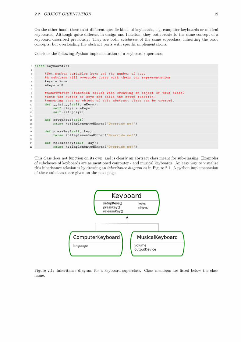
This class does not function on its own, and is clearly an abstract class meant for sub-classing. Examplesof subclasses of keyboards are as mentioned computer - and musical keyboards. An easy way to visualizethis inheritance relation is by drawing an inheritance diagram as in Figure 2.1. A python implementationof these subclasses are given on the next page.
KeyboardkeysnKeys
setupKeys()pressKey()releaseKey()
ComputerKeyboard
language
MusicalKeyboard
volumeoutputDevice
Figure 2.1: Inheritance diagram for a keyboard superclass. Class members are listed below the classname.
20 CHAPTER 2. SCIENTIFIC PROGRAMMING
1 #The (keyboard) spesifies inheritance from Keyboard
2 class ComputerKeyboard(Keyboard):
3
4 def __init__(self, language , nKeys):
5
6 self.language = language
7
8 #Use the superclass contructor to set the number of keys
9 super(ComputerKeyboard , self).__init__(nKeys)
10
11
12 def setupKeys(self):
13
14 if self.language == "Norwegian":
15 "Set up norwegian keyboard style"
16 elif ...
17
18
19 def pressKey(self, key):
20 return self.keys[key]
21
22
23
24 #Dummy import for illustration purposes
25 from myDevices import Speakers
26
27 class MusicalKeyboard(Keyboard):
28
29 def __init__(self, nKeys , volume):
30
31 #Set the ouput device to speakers implemented elsewhere
32 self.outputDevice = Speakers ()
33 self.volume = volume
34
35 super(ComputerKeyboard , self).__init__(nKeys)
36
37
38 def setupKeys(self):
39 lowest = 27.5 #Hz
40 step = 1.06 #Relative increase in Hz (neighbouring keys)
41
42 self.keys = [lowest + i*step for i in range(self.nKeys)]
43
44
45 def pressKey(self, key):
46
47 #Returns a harmonic wave with frequency and amplitude
48 #extracted from the pressed key and the volume level.
49 outout = ...
50 self.outputDevice.play(key , output)
51
52
53 #Fades out the playing tune
54 def releaseKey(self, key):
55 self.outputDevice.fade(key)
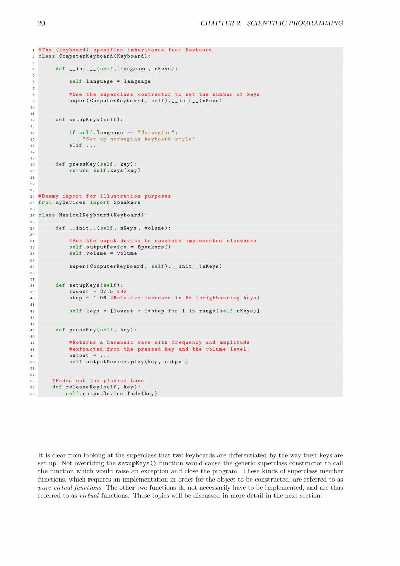
It is clear from looking at the superclass that two keyboards are differentiated by the way their keys areset up. Not overriding the setupKeys() function would cause the generic superclass constructor to callthe function which would raise an exception and close the program. These kinds of superclass memberfunctions, which requires an implementation in order for the object to be constructed, are referred to aspure virtual functions. The other two functions do not necessarily have to be implemented, and are thusreferred to as virtual functions. These topics will be discussed in more detail in the next section.
2.2. OBJECT ORIENTATION 21
2.2.3 Pointers, Typecasting and Virtual Functions
A pointer is a hexadecimal number representing a memory address where some type of object is stored,for instance, an int at 0x7fff0882306c (0x simply implies hexadecimal). Higher level languages likePython handles all the pointers and typesetting automatically. In low-level languages like C++, however,you need to control everything. This is commonly referred to as type safety.
Memory addresses are global, that is, they are shared throughout the program. This implies that changesdone to a pointer to an object, e.g. Keyboard* myKeyboard, are applied everywhere the object is in use.This is particularly handy (or dangerous) when passing a pointer as an argument to a function, as changesapplied to the given object will cause the object to remain changed after exiting the function. Passingnon-pointer arguments would only change a local copy of the object which is destroyed upon exiting thefunction. The alternative would be to pass the reference to the object, e.g. &myObject, which passes theaddress just as in the case of pointers.
Creating a pointer to a keyboard object in C++ can be done in several ways. Following are threeexamples:
1 MusicalKeyboard* myKeyboard1 = new MusicalKeyboard (...);
2 Keyboard* myKeyboard2 = new MusicalKeyboard (...);
the second which is identical to
1 Keyboard* myKeyboard2 = (Keyboard *) myKeyboard1;
For reasons which will be explained in Section 2.2.4, the second expression is extremely handy. Technically,the subclass object is type cast to the superclass type. This is allowed since any subclass is type-compatiblewith a pointer to it’s superclass. Any standard functions implemented in the subclass will not be directlycallable from outside the object itself, and identical functions will be overwritten by the correspondingsuperclass functions, unless the functions are virtual. Flagging a function as virtual in the superclass willthen tell the compiler not to overwrite this particular function when a subclass object is typecast to thesuperclass type.
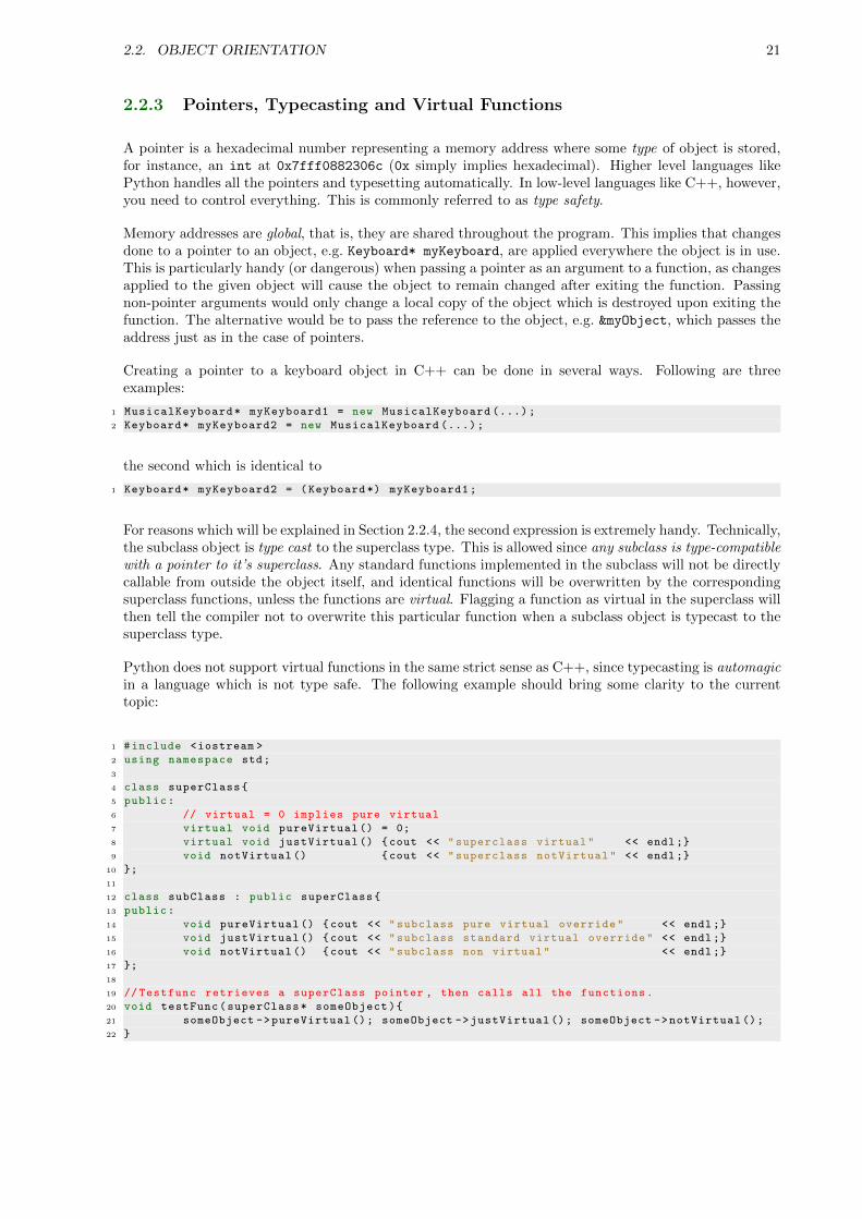
Python does not support virtual functions in the same strict sense as C++, since typecasting is automagicin a language which is not type safe. The following example should bring some clarity to the currenttopic:
1 #include <iostream >
2 using namespace std;
3
4 class superClass{
5 public:
6 // virtual = 0 implies pure virtual
7 virtual void pureVirtual () = 0;
8 virtual void justVirtual () {cout << "superclass virtual" << endl;}
9 void notVirtual () {cout << "superclass notVirtual" << endl;}
10 };
11
12 class subClass : public superClass{
13 public:
14 void pureVirtual () {cout << "subclass pure virtual override" << endl;}
15 void justVirtual () {cout << "subclass standard virtual override" << endl;}
16 void notVirtual () {cout << "subclass non virtual" << endl;}
17 };
18
19 // Testfunc retrieves a superClass pointer , then calls all the functions.
20 void testFunc(superClass* someObject){
21 someObject ->pureVirtual (); someObject ->justVirtual (); someObject ->notVirtual ();
22 }
22 CHAPTER 2. SCIENTIFIC PROGRAMMING
1 int main(){
2
3 cout << "-Calling subClass object of type superClass*" << endl;
4 superClass* object = new subClass (); testFunc(object);
5
6 cout << endl << "-Calling subClass object of type subClass*" << endl;
7 subClass* object2 = new subClass (); testFunc(object);
8
9 cout << endl << "-Directly calling object of type subclass*" << endl;
10 object2 ->pureVirtual (); object2 ->justVirtual (); object2 ->notVirtual ();
11
12 return 0;
13 }
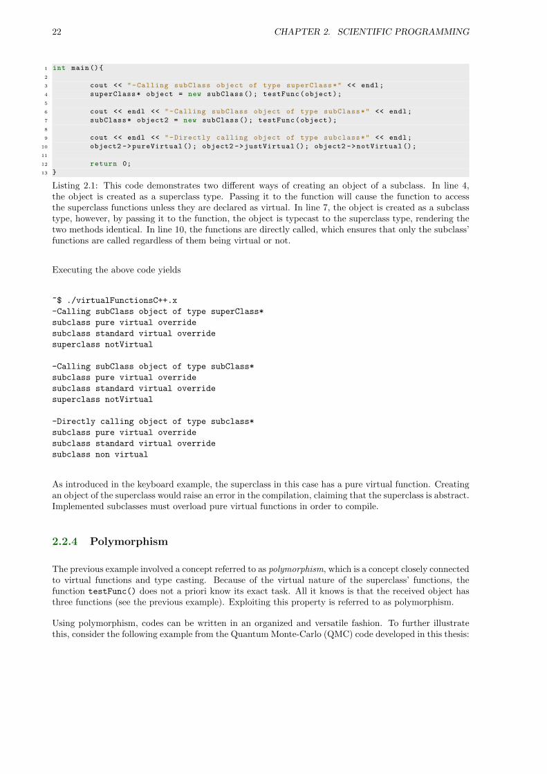
Listing 2.1: This code demonstrates two different ways of creating an object of a subclass. In line 4,the object is created as a superclass type. Passing it to the function will cause the function to accessthe superclass functions unless they are declared as virtual. In line 7, the object is created as a subclasstype, however, by passing it to the function, the object is typecast to the superclass type, rendering thetwo methods identical. In line 10, the functions are directly called, which ensures that only the subclass’functions are called regardless of them being virtual or not.
Executing the above code yields
~$ ./virtualFunctionsC++.x
-Calling subClass object of type superClass*
subclass pure virtual override
subclass standard virtual override
superclass notVirtual
-Calling subClass object of type subClass*
subclass pure virtual override
subclass standard virtual override
superclass notVirtual
-Directly calling object of type subclass*
subclass pure virtual override
subclass standard virtual override
subclass non virtual
As introduced in the keyboard example, the superclass in this case has a pure virtual function. Creatingan object of the superclass would raise an error in the compilation, claiming that the superclass is abstract.Implemented subclasses must overload pure virtual functions in order to compile.
2.2.4 Polymorphism
The previous example involved a concept referred to as polymorphism, which is a concept closely connectedto virtual functions and type casting. Because of the virtual nature of the superclass’ functions, thefunction testFunc() does not a priori know its exact task. All it knows is that the received object hasthree functions (see the previous example). Exploiting this property is referred to as polymorphism.
Using polymorphism, codes can be written in an organized and versatile fashion. To further illustratethis, consider the following example from the Quantum Monte-Carlo (QMC) code developed in this thesis:

2.2. OBJECT ORIENTATION 23
1 class Potential {
2 protected:
3 int n_p;
4 int dim;
5
6 public:
7 Potential(int n_p , int dim);
8
9 //Pure virtual function
10 virtual double get_pot_E(const Walker* walker) const = 0;
11
12 };
13
14 class Coulomb : public Potential {
15 public:
16
17 Coulomb(GeneralParams &);
18
19 // Returns the sum 1/r_i
20 double get_pot_E(const Walker* walker) const;
21
22 };
23
24 class Harmonic_osc : public Potential {
25 protected:
26 double w;
27
28 public:
29
30 Harmonic_osc(GeneralParams &);
31
32 // return the sum 0.5*w*r_i^2
33 double get_pot_E(const Walker* walker) const;
34
35 };
36
37 ...
Listing 2.2: An example from the QMC code. The superclass of potentials is defined by a number ofparticles (line 3), a dimension (line 4) and a pure virtual function for extracting the local energy of a givenwalker (line 10). Specific potentials are implemented as subclasses (line 14 and 24), simply overridingthe pure virtual function with their own implementations.
Assume that an object Potential* potential is sent to an energy function. Since get_pot_E() isvirtual, the potential can take any form; the energy function only checks whether it has an implementationor not. The code can easily be adapted to handle any combination of any potentials by storing thepotential objects in a vector and simply accumulate the contributions:
1 // Simple compiler definition to clean up the code
2 #define potvec std::vector <Potential*>
3
4 class System {
5
6 double get_potential_energy(const Walker* walker) const;
7 potvec potentials;
8 ...
9 };
10
11 double System :: get_potential_energy(const Walker* walker) const {
12 double potE = 0;
13
14 // Iterates through all loaded potentials and accumulate energies.
15 for (potvec :: iterator pot = potentials.begin (); pot != potentials.end(); ++pot) {
16 potE += (*pot)->get_pot_E(walker);
17 }
18
19 return potE;
20 }
24 CHAPTER 2. SCIENTIFIC PROGRAMMING
2.2.5 Const Correctness
In the previous Potential code example, function declarations with the const flag were used. Asmentioned in the section on pointers, passing pointers to functions are dangerous business. If an objectis flagged with const on input, e.g. void f(const x), the function itself cannot alter the value of x. If itdoes, the compiler will abort. This property is referred to as const correctness, and serve as a safeguardguaranteeing that nothing will happen to x as it passes through f. This is practical in situations wherechanges to an object are unwanted.
If you declare a member function itself with const on the right hand side, e.g. void class::f(x) const,no changes may be applied to class members inside this specific function. For instance, in the potentialenergy functions, all that is requested is to evaluate a function at a given set of coordinates; there is noneed to change anything, hence the const correctness is applied to the function.
In other words: const correctness works as a safeguard preventing changes to values which should remainunchanged. A change in such a variable is then followed by a compiler error instead of unforeseenconsequences.
2.2.6 Accessibility levels and Friend classes
When a C++ class is declared, each member needs to be related to an accessibility level. The threeaccessibility levels in C++ are
(i) Public: The variable or function may be accessed from anywhere the object is available.
(ii) Private: The variable or function may be accessed only from within the class itself.
(iii) Protected: As for private, but also accessible from subclasses of the class.
As an example, any standardized application (app) needs the app::execute_app() function to be public,i.e. accessible from the main file. On the other hand, app::dump_progress() should be controlled bythe application itself, and should thus be private, or protected in case the application has subclasses.
There is one exception to the rule of protected - and private variables. In certain situations where a classneeds to access private variables from another class, but going full public is undesired, the latter class canfriend the first class. This implies that the first class has access to the second class’ private members.
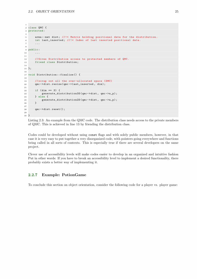
In the QMC code developed in this thesis, the distribution is calculated by a class Distrubution. Inorder to achieve this, the protected members of QMC need to be made available to the Distrubution class.This is implemented in the following fashion:
2.2. OBJECT ORIENTATION 25
1
2 class QMC {
3 protected:
4
5 arma::mat dist; //!< Matrix holding positional data for the distribution.
6 int last_inserted; //!< Index of last inserted positional data.
7 ...
8
9 public:
10 ...
11
12 //Gives Distribution access to protected members of QMC.
13 friend class Distribution;
14
15 };
16
17 void Distribution :: finalize () {
18
19 //scrap out all the over -allocated space (DMC)
20 qmc ->dist.resize(qmc ->last_inserted , dim);
21
22 if (dim == 3) {
23 generate_distribution3D(qmc ->dist , qmc ->n_p);
24 } else {
25 generate_distribution2D(qmc ->dist , qmc ->n_p);
26 }
27
28 qmc ->dist.reset();
29
30 }
Listing 2.3: An example from the QMC code. The distribution class needs access to the private membersof QMC. This is achieved in line 13 by friending the distribution class.
Codes could be developed without using const flags and with solely public members, however, in thatcase it is very easy to put together a very disorganized code, with pointers going everywhere and functionsbeing called in all sorts of contexts. This is especially true if there are several developers on the sameproject.
Clever use of accessibility levels will make codes easier to develop in an organized and intuitive fashionPut in other words: If you have to break an accessibility level to implement a desired functionality, thereprobably exists a better way of implementing it.
2.2.7 Example: PotionGame
To conclude this section on object orientation, consider the following code for a player vs. player game:
26 CHAPTER 2. SCIENTIFIC PROGRAMMING
1 #playerClass.py
2 import random
3
4 class Player:
5
6 def __init__(self, name):
7 #Player initialized at full health and full energy.
8 self.health = self.energy = 100
9
10 self.name = name
11 self.dead = False
12
13 #Player initialized with no available potions.
14 self.potions = []
15
16
17 def addPotion(self, potion):
18 self.potions.append(potion)
19
20
21 #Selects the given potion and consumes it. The potion needs to know
22 #the player it should affect , hence we send ’self’ as an argument.
23 def usePotion(self, potionIndex):
24 print "%s consumes %s." % (self.name , self.potions[potionIndex ].name)
25
26 selectedPotion = self.potions[potionIndex]
27 selectedPotion.applyPotionTo(self) #Self explainatory!
28 self.potions.pop(potionIndex) #Removed the potion.
29
30
31 def changeHealth(self, amount):
32 self.health += amount
33
34 #Cap health at [0 ,100].
35 if self.health > 100: self.health = 100
36 elif self.health <= 0:
37 self.health = 0
38 self.dead = True;
39
40
41 def changeEnergy(self, amount):
42 self.energy += amount
43
44 #Cap energy at [0 ,100].
45 if self.energy > 100: self.energy = 100
46 elif self.energy < 0: self.energy = 0
47
48
49 #Lists the potions to the user.
50 def displayPotions(self):
51 if not self.potions:
52 print " No potions available"
53
54 for potion in self.potions: print " " + potion.name
55
56
57 def attack(self, targetPlayer):
58
59 energyCost = 55
60
61 if self.energy < energyCost:
62 print "%s: Insuficcient energy to attack." % self.name; return
63
64 damage = 40 + random.randint (-10, 10)
65
66 targetPlayer.changeHealth(-damage)
67 self.changeEnergy(-energyCost)
68
69 print "%s hit %s for %s using %s energy" % (self.name ,
70 targetPlayer.name ,
71 damage , energyCost)

2.2. OBJECT ORIENTATION 27
1 #potionClass.py
2
3 class Potion:
4
5 def __init__(self, amount):
6 self.amount = amount
7 self.setName ()
8
9 def applyPotionTo(self, player):
10 raise NotImplementedError("Member function applyPotion not implemented.")
11
12 #This function should be overwritten
13 def setName(self):
14 self.name = "Undefined"
15
16
17 class HealthPotion(Potion):
18
19 #Constructor is inherited
20
21 #Calls back to the player object ’s functions to change the health
22 def applyPotionTo(self, player):
23 player.changeHealth(self.amount)
24
25 def setName(self):
26 self.name = "Health Potion (%d)" % self.amount
27
28
29 class EnergyPotion(Potion):
30
31 def applyPotionTo(self, player):
32 player.changeEnergy(self.amount)
33
34 def setName(self):
35 self.name = "Energy Potion (%d)" % self.amount
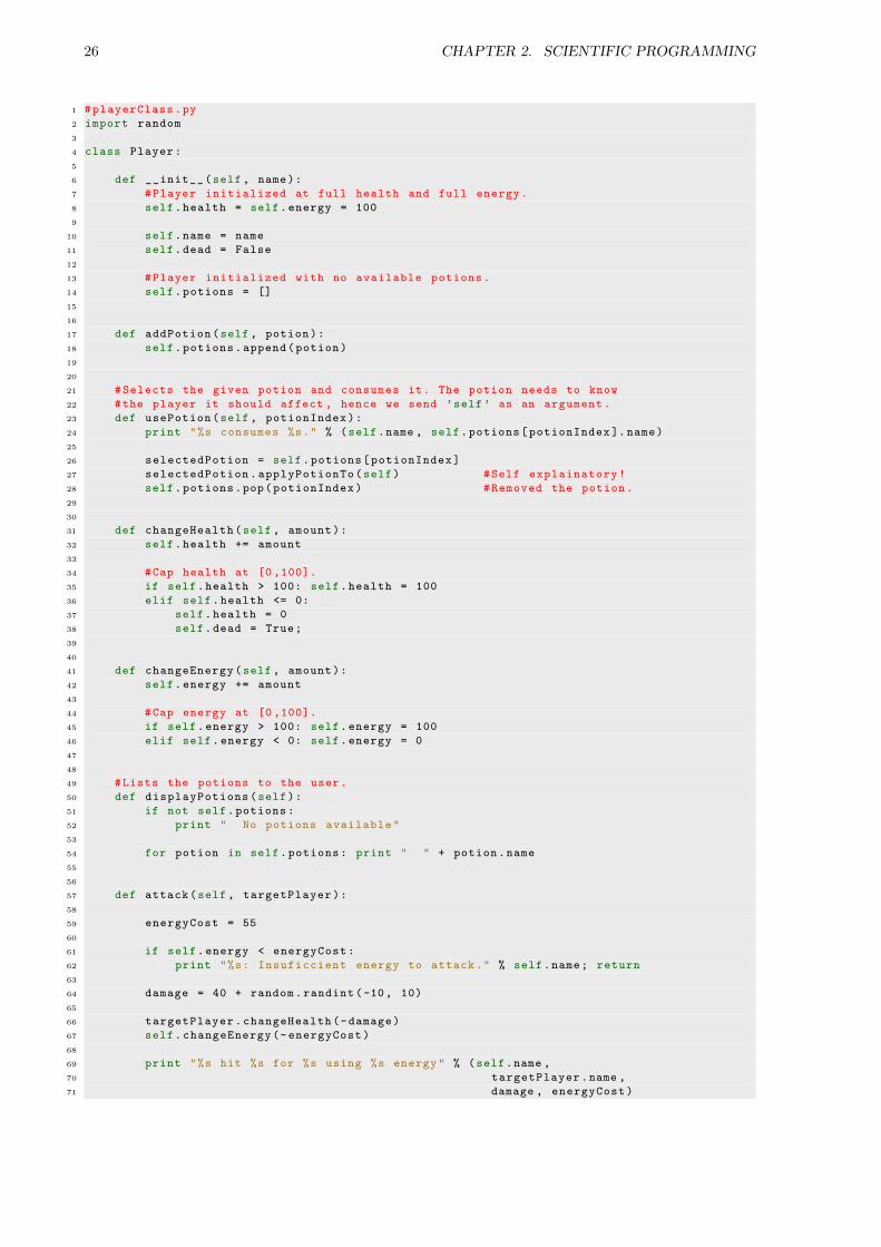
The Player class keeps track of everything a player needs of personal data, such as the name (line 10),health- and energy levels (line 8), potions etc. Bringing another player into the game is simply done bycreating another Player object. A player holds a number of Potion objects in a list (line 14). Theseobjects are subclass implementations of the abstract potion class, which overwrites the virtual functiondescribing the potion’s effect on a given player object. This is demonstrated in lines 23 and 32. Thissubclass hierarchy of potions makes it incredibly easy to implement new ones.
The power of object orientation shines through in this simple example. The readability is very good, anddoes not falter if numerous potions or players are brought to the table.
In this section the focus has not been solely on scientific computing, but rather on the use of objectorientation in general. The interplay between the potions and the players in the current example closelyresembles the interplay between the QMC solver and the potentials introduced previously. Whethergames or scientific programs are at hand, the methods used in the programming remain the same.
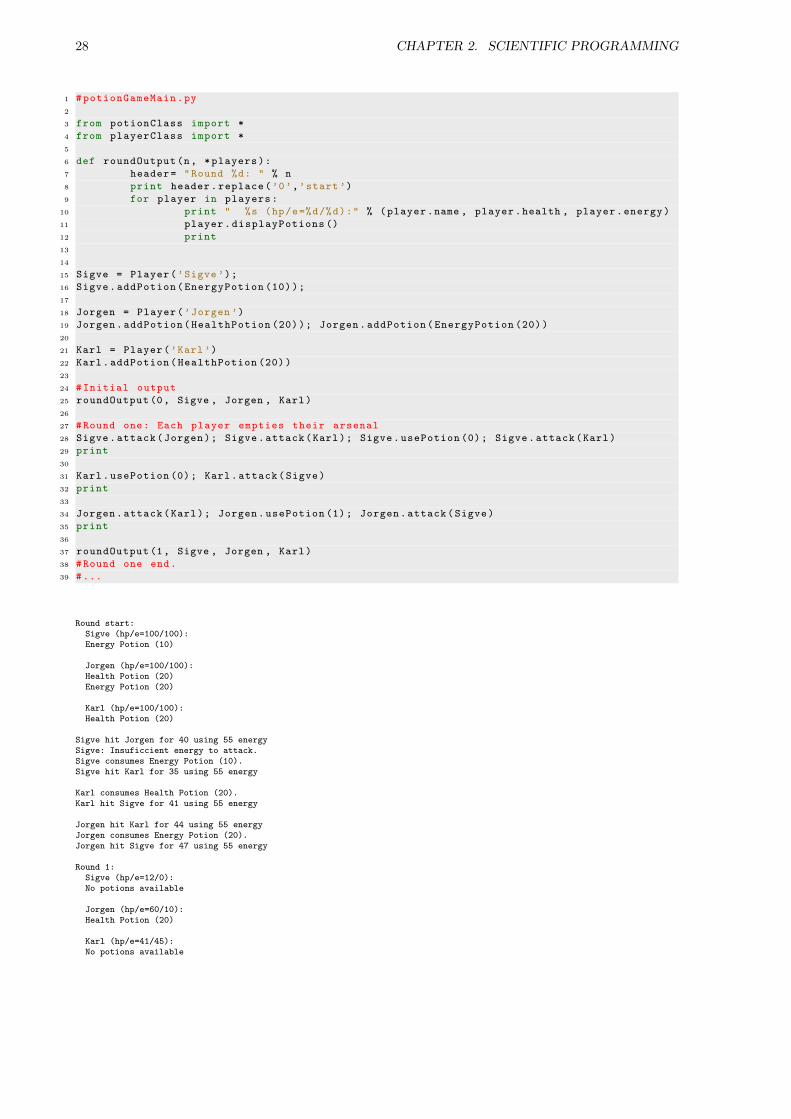
On the following page, a game is constructed using the Player and Potion classes. In lines 15-22, threeplayers are initialized with a set of potions, from where they battle each other one round. The syntaxis extremely transparent. Adding a fourth player is simply a matter of adding a new line of code. Theoutput of the game is displayed below the code.
28 CHAPTER 2. SCIENTIFIC PROGRAMMING
1 #potionGameMain.py
2
3 from potionClass import *
4 from playerClass import *
5
6 def roundOutput(n, *players):
7 header= "Round %d: " % n
8 print header.replace(’0’,’start’)
9 for player in players:
10 print " %s (hp/e=%d/%d):" % (player.name , player.health , player.energy)
11 player.displayPotions ()
12 print
13
14
15 Sigve = Player(’Sigve’);
16 Sigve.addPotion(EnergyPotion (10));
17
18 Jorgen = Player(’Jorgen ’)
19 Jorgen.addPotion(HealthPotion (20)); Jorgen.addPotion(EnergyPotion (20))
20
21 Karl = Player(’Karl’)
22 Karl.addPotion(HealthPotion (20))
23
24 #Initial output
25 roundOutput (0, Sigve , Jorgen , Karl)
26
27 #Round one: Each player empties their arsenal
28 Sigve.attack(Jorgen); Sigve.attack(Karl); Sigve.usePotion (0); Sigve.attack(Karl)
29 print
30
31 Karl.usePotion (0); Karl.attack(Sigve)
32 print
33
34 Jorgen.attack(Karl); Jorgen.usePotion (1); Jorgen.attack(Sigve)
35 print
36
37 roundOutput (1, Sigve , Jorgen , Karl)
38 #Round one end.
39 #...
Round start:Sigve (hp/e=100/100):Energy Potion (10)
Jorgen (hp/e=100/100):Health Potion (20)Energy Potion (20)
Karl (hp/e=100/100):Health Potion (20)
Sigve hit Jorgen for 40 using 55 energySigve: Insuficcient energy to attack.Sigve consumes Energy Potion (10).Sigve hit Karl for 35 using 55 energy
Karl consumes Health Potion (20).Karl hit Sigve for 41 using 55 energy
Jorgen hit Karl for 44 using 55 energyJorgen consumes Energy Potion (20).Jorgen hit Sigve for 47 using 55 energy
Round 1:Sigve (hp/e=12/0):No potions available
Jorgen (hp/e=60/10):Health Potion (20)
Karl (hp/e=41/45):No potions available
2.3. STRUCTURING THE CODE 29
2.3 Structuring the code
Structuring a code is a matter of making choices based on the complexity of the code. If the code is shortand has a direct purpose, for instance, to calculate the sum from Eq. (2.1), the structure is not an issue atall, given that reasonable variable names are used. However, if the code is more complex and the methodsused are specific implementations of a more general case, e.g. potentials, code structuring becomes veryimportant. For details about the structuring of the code used in this thesis, see the documentationprovided in Ref. [9].
2.3.1 File Structures
Not only does the potion game example demonstrate clean object orientation, but also standard filestructuring by splitting the different classes and the main application into separate files. In a small code,like for example the potion game, the gain of transparency is not immense, however, when the classstructures span thousands of lines, having a good structure is crucial to the development process, thecode’s readability, and the management in general.
Developing codes in scientific scenarios often involve large frameworks. For example, when coding molec-ular dynamics, several collision models, force models etc. are implemented alongside the main solver.In the case of Markow Chain Monte Carlo methods, different diffusion models (sampling rules) may beselectable. Even though these models are implemented using polymorphism, the code still gets messywhen the amount of classes gets large.
In these scenarios, it is common to gather the implementations of the different classes in separate files(as for the potion game). This would be for purely cosmetic reasons if the process of writing code waslinear, however, empirical evidence suggests otherwise: At least half the time is spent debugging, goingback and forth between files.
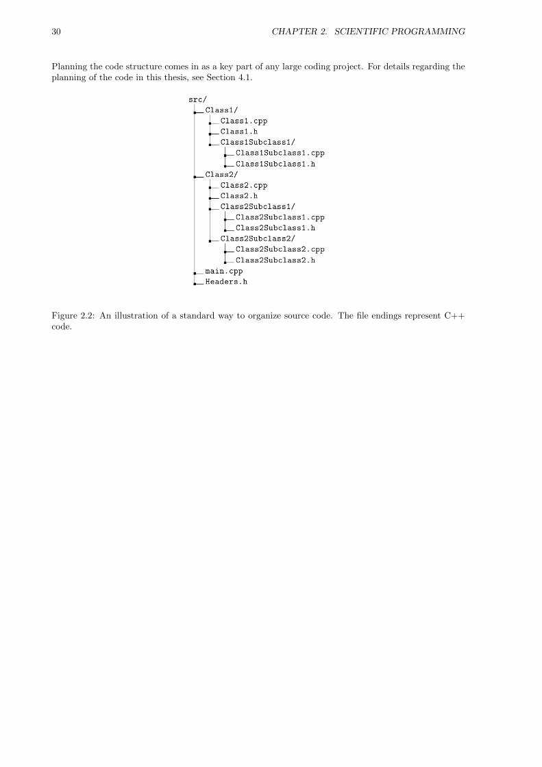
A standard way to organize code is to have all the source code gathered in an src folder, with one folderper distinct class. Subclasses should appear as folders inside the superclass folder. Figure 2.2 shows anexample setup for the framework of an object oriented code.
Another gain by this structuring files this way, is that tools such as Make, QMake, etc. ensures that onlythe files that actually changed will be recompiled. This saves a lot of time in the development processonce the total compilation time starts taking several minutes.
2.3.2 Class Structures
In scientific programming, the simulated process often has a physical or mathematical interpretation.Some examples are, for instance, atoms in molecular dynamics and Bose-Einstein condensates, randomwalkers in diffusion processes, etc. Implementing classes representing these quantities will shorten thegap between the mathematical formulation of the problem and the implementation.
In addition, quantities such as the energy, entropy and temperature, are all calculated based on equationsfrom statistical mechanics, quantum mechanics, or similar. Having class methods representing these calcu-lations will again shorten the gap. There is no question what is done when the system::get_potential_Emethod is called, however, if some random loop appears in the main solver, an initial investigation isrequired in order to understand the flow of the code.
As described in Section 2.2.4, abstracting for example the potential energy function into a system objectopens up the possibility of generalizing the code to any potential without altering the main solver.Structure is in other words vital if readability and versatility is desired.
30 CHAPTER 2. SCIENTIFIC PROGRAMMING
Planning the code structure comes in as a key part of any large coding project. For details regarding theplanning of the code in this thesis, see Section 4.1.
Figure 2.2: An illustration of a standard way to organize source code. The file endings represent C++code.
3
Quantum Monte-Carlo
Quantum Monte-Carlo (QMC) is a method for solving Schrodinger’s equation using statistical MarkovChain (random walk) simulations. The statistical nature of Quantum Mechanics makes Monte-Carlomethods the perfect tool not only for accurately estimating observables, but also for extracting interestingquantities such as densities, i.e. probability distributions.
There are multiple strategies which can be used in order to deduce the virtual1 dynamics of QMC, someof which are more mathematically complex than others. In this chapter the focus will be on modellingthe Schrodinger equation as a diffusion problem in complex (Wick rotated) time. Other more condensedmathematical approaches does not need the Schrodinger equation at all, however, for the purpose ofcompleteness, this approach will be mentioned only briefly in Section 3.2.3.
In this chapter, Dirac Notation will be used. See Appendix A for an introduction. The equations willbe in atomic units, i.e. ~ = me = e = 4πε0 = 1, where me and ε0 are the electron mass and the vacuumpermittivity, respectively.
3.1 Modelling Diffusion
Like any phenomena involving a probability distribution, Quantum Mechanics can be modelled by adiffusion process. In Quantum Mechanics, the distribution is given by |Φ(r, t)|2, the wave functionsquared. The diffusing elements of interest are the particles in the system at hand.
The basic idea is to introduce an ensemble of random walkers, in which each walker is represented by aposition in space at a given time. Once the walkers reach equilibrium, averaging values over the pathsof the ensemble will yield average values corresponding to the probability distribution governing themovement of individual walkers. In other words: Counting every walker’s contribution within a smallvolume dr will correspond to |Φ(r, t)|2dr in the limit of infinite walkers.
Such random movement of walkers are referred to as a Brownian motion, named after the British botanistR. Brown, originating from his experiments on plant pollen dispersed in water. Markov chains are asubtype of Brownian motion, where a walkers next move is independent of previous moves. This is thestochastic process in which QMC is described.
1As will be shown, the time parameter in QMC does not correspond to physical time, but rather an imaginary axis at afixed point in time. Whether nature operates on a complex time plane or not is not testable in a laboratory, and the originof the probabilistic nature of Quantum Mechanics will thus remain a philosophical problem.
31
32 CHAPTER 3. QUANTUM MONTE-CARLO
The purpose of this section is to motivate the use of diffusion theory in Quantum Mechanics, and toderive the sampling rules needed in order to model Quantum Mechanical distributions by diffusion ofrandom walkers correctly.
3.1.1 Stating the Schrodinger Equation as a Diffusion Problem
Consider the time-dependent Schrodinger equation for an arbitrary wave function Φ(r, t) using an arbi-trary energy shift E′
− ∂Φ(r, t)
i∂t= (H− E′)Φ(r, t). (3.1)
Given that the Hamiltonian is time-independent, the formal solution is found by separation of variablesin Φ(r, t) [17]
HΦ(r, t0) = EΦ(r, t0), (3.2)
Φ(r, t) = exp(−i(H− E′)(t− t0)
)Φ(r, t0). (3.3)
From Eq. (3.3) it is apparent that the time evolution operator is on the form
U(t, t0) = exp(−i(H− E′)(t− t0)
). (3.4)
The time-independent equation is solved for the ground state energy through methods such as FullConfiguration Interaction [18] or similar methods based on diagonalizing the Hamiltonian. The time-dependent equation is used by methods such as Time-Dependent Multi-Configuration Hartree-Fock [19]in order to obtain the time-development of quantum states. However, neither of the equations originatefrom, or resemble, diffusion equations.
The original Schrodinger equation, however, does resemble a diffusion equation in complex time2. It cannot be treated as a true diffusion equation, since the time evolved quantity, the wave function, is nota probability distribution unless it is squared. However, the equation involves a time derivative and aLaplacian, strongly indicating some sort of connection to a diffusion process.
Substituting complex time with a parameter τ and choosing the energy shift E′ equal to the true groundstate energy of H, E0, the time evolution operator in Eq. (3.4) becomes the projection operation P(τ),whose choice of name will soon be apparent. In other words:
t→ it ≡ τ,
U(t, 0)→ exp(−(H− E0)τ
)≡ P(τ).
Consider an arbitrary wave function ΨT (r). Applying the new operator yields a new wave function Φ(r, τ)in the following manner
2The physical time diffusion equation evolves the squared wave function, and can be deduced from the quantum continuityequation combined with Fick’s laws of diffusion [20].

3.1. MODELLING DIFFUSION 33
Φ(r, τ) = 〈r| P(τ) |ΨT 〉 (3.5)
= 〈r| exp(−(H− E0)τ
)|ΨT 〉 .
Expanding the arbitrary state in the eigenfunction of H, |Ψi〉, yields
Φ(r, τ) =∑i
Ci 〈r| exp(−(H− E0)τ
)|Ψi〉
=∑i
CiΨi(r) exp (−(Ei − E0)τ)
= C0Ψ0(x) +
∞∑i=1
CiΨk(x)e−δEiτ , (3.6)
where Ci = 〈Ψi|ΨT 〉 and δEi = Ei − E0 ≥ 0. In the limit where τ goes to infinity, the ground state isthe sole survivor of the expression, hence the name projection operator. In other words:
limτ→∞
Φ(r, τ) = limτ→∞
〈r| P(τ) |ΨT 〉
= C0Ψ0(x). (3.7)
The projection operator transforms an arbitrary wave function ΨT (r), from here on referred to as thetrial wave function, into the true ground state, given that the overlap C0 is non-zero.
In order to model the projection with Markov chains, the process needs to be split into subprocesses whichin turn can be described as transitions in the Markov chain. Introducing a time-step δτ , the projectionoperator can be rewritten as
P(τ) =
n∏k=1
exp(−(H− E0)δτ
), (3.8)
where n = τ/δτ . An important property to notice is that
P(τ + δτ) = exp(−(H− E0)δτ
)P(τ). (3.9)
Using this relation in combination with Eq. (3.5), the effect of the projection operator during a singletime-step is revealed:
Φ(r, τ + δτ) = 〈r| P(τ + δτ) |ΨT 〉
= 〈r| exp(−(H− E0)δτ
)P(τ) |ΨT 〉
= 〈r| exp(−(H− E0)δτ
)|Φ(τ)〉
=
∫r′〈r| exp
(−(H− E0)δτ
)|r′〉 〈r′|Φ(τ)〉dr′
=
∫r′〈r| exp
(−(H− E0)δτ
)|r′〉Φ(r′, τ)dr′, (3.10)
34 CHAPTER 3. QUANTUM MONTE-CARLO
where a complete set of position states were introduced.
For practical purposes, E0 needs to be substituted with an approximation ET to the ground state energy,commonly referred to as the trial energy, in order to avoid self consistency. From Eq. (3.6) it is apparentthat the projection will still converge as long as ET < E1, that is, the trial energy is less than that of thefirst excitation. The resulting expression reads:
Φ(r, τ + δτ) =
∫r′〈r| exp
(−(H− ET )δτ
)|r′〉Φ(r′, τ)dr′ (3.11)
≡∫r′G(r, r′; δτ)Φ(r′, τ)dr′. (3.12)
The equations above are well suited for Markov Chain models, as an ensemble of walkers can be iteratedby transitioning between configurations |r〉 and |r′〉 with probabilities given by the Green’s function,G(r, r′; δτ).
The effect of the Green’s function from Eq. (3.12) on individual walkers is not trivial. In order to relatethe Green’s function to well-known processes, the exponential is split into two parts, one containing onlythe kinetic energy operator T = − 1
2∇2, and the second containing the potential energy operator V and
the energy shift. This is known as the short time approximation [21]
G(r, r′; δτ) = 〈r| exp(−(H− ET )δτ
)|r′〉 (3.13)
= 〈r| e−Tδτe−(V−ET )δτ |r′〉+1
2[V, T]δτ2 +O(δτ3). (3.14)
The first exponential describes a transition of walkers governed by the Laplacian, which is a diffusionprocess. The second exponential is linear in position space and is thus a weighing function responsiblefor distributing the correct weights to the corresponding walkers. In other words:
GDiff = e12∇
2δτ , (3.15)
GB = e−(V−ET )δτ , (3.16)
where B denotes branching. The reasons for this name together with the complete process of modellingweights by branching will be covered in detail in Section 3.5.
The flow of QMC is then to use these Green’s functions to propagate the ensemble of walkers intothe next time-step. The final distribution of walkers will correspond to that of the direct solution ofthe Schrodinger equation, given that the time-step is sufficiently small, and the number of cycles n aresufficiently large. These constraints will be covered in more detail later.
Incorporating only the effect of Eq. (3.15) results in a method called Variational Monte-Carlo (VMC).Including the branching term as well results in Diffusion Monte-Carlo (DMC). These methods will bediscussed in Sections 3.8 and 3.9, respectively. In either of these methods, diffusion is a key process.
3.2 Solving the Diffusion Problem
The diffusion problem introduced in the previous section uses a symmetric kinetic energy operator im-plying an isotropic diffusion, however, a more efficient kinetic energy operator can be introduced without
3.2. SOLVING THE DIFFUSION PROBLEM 35
violating the original equations, resulting in an anisotropic diffusion governed by the Fokker-Planckequation. These models will be the topic of this section.
For details regarding the transition from isotropic to anisotropic diffusion, see Section 3.2.3.
3.2.1 Isotropic Diffusion
Isotropic diffusion is a process in which diffusing particles sees all directions as an equally probable path.Eq. (3.17) is an example of this. The isotropic diffusion equation is
∂P (r, t)
∂t= D∇2P (r, t). (3.17)
This is the simplest form of a diffusion equation, that is, the case with a linear diffusion constant, D, andno drift terms.
From Eq. (3.15) it is clear that the value of the diffusion constant is D = 12 , originating from the term
scaling the Laplacian in the Schrodinger Equation. An important point is that closed form expressions forthe Green’s function exists. This closed form expression in the isotropic case is a Gaussian distributionwith variance 2Dδt [21]
GISODiff(i → j) ∝ e−|ri−rj |
2/4Dδτ . (3.18)
These equations describe the diffusion process theoretically, however, in order to achieve specific sam-pling rules for the walkers, a connection between the time-dependence of the distribution and the time-dependence of an individual walker’s components in configuration space is needed. This connection isgiven in terms of a stochastic differential equation called The Langevin Equation.
The Langevin Equation for isotropic diffusion
The Langevin Equation is a stochastic differential equation used in physics to relate the time dependenceof a distribution to the time-dependence of the degrees of freedom in a system. For isotropic diffusion,solving the Langevin equation using a Forward Euler approximation for the time derivative results in thefollowing relation:
xi+1 = xi + ξ, Var(ξ) = 2Dδt, (3.19)
〈ξ〉 = xi,
where ξ is a normal distributed number whose variance matches that of the Green’s function in Eq. (3.18).This relation is in agreement with the isotropy of Eq. (3.17) in the sense that the displacement is symmetricaround the current position.
3.2.2 Anisotropic Diffusion and the Fokker-Planck equation
Anisotropic diffusion, in contrast to isotropic diffusion, does not see all directions as equally probable. Anexample of this is diffusion according to the Fokker-Planck Equation, that is, diffusion with a drift term,F(r, t), responsible for pushing the walkers in the direction of configurations with higher probabilities,and thus closer to an equilibrium state. The Fokker-Planck equation reads:
36 CHAPTER 3. QUANTUM MONTE-CARLO
∂P (r, t)
∂t= D∇ ·
[(∇− F(r, t)
)P (r, t)
]. (3.20)
As will be derived in detail in Section 3.2.3, using the Fokker-Planck equation does not violate the originalSchrodinger equation, but changes the representation of the ensemble of walkers to a mixed density. Thismeans that QMC can be run with Fokker-Planck diffusion, leading to a more optimized way of samplingdue to the drift term.
As mentioned introductory, the goal of the Markov process is convergence to a stationary state. Usingthis criteria, the expression for the drift term can be found. A stationary state is obtained when the lefthand side of Eq. (3.20) is zero. This yields:
∇2P (r, t) = P (r, t)∇ · F(r, t) + F(r, t) · ∇P (r, t).
In order to get cancellation in the remaining terms, the Laplacian term on the right-hand side must cancelout the terms on the left. This implies that the drift term needs to be on the form F(r, t) = g(r, t)∇P (r, t).Inserting this yields
∇2P (r, t) = P (r, t)∂g(r, t)
∂P (r, t)
∣∣∣∇P (r, t)∣∣∣2 + P (r, t)g(r, t)∇2P (r, t) + g(r, t)
∣∣∣∇P (r, t)∣∣∣2.
The factors in front of the Laplacian suggests using g(r, t) = 1/P (r, t). A quick check reveals that thisalso cancels the gradient terms. The resulting expression for the drift term becomes
F(r, t) =1
P (r, t)∇P (r, t)
=2
|ψ(r, t)|∇|ψ(r, t)|. (3.21)
In QMC, the drift term is commonly referred to as the quantum force. This is due to the fact that it isresponsible for pushing the walkers into regions of higher probabilities, analogous to a force in Newtonianmechanics.
Another strength of the Fokker-Planck equation is that even though the equation itself is more compli-cated, its Green’s function still has a closed form solution. This means that it can be evaluated efficiently.If this was not the case, the practical value would be reduced dramatically. The reason for this will becomeclear in Section 3.4. The closed form solution reads [21]
GFPDiff(i → j) ∝ e−(xi−xj−DδτF (xi))
2/4Dδτ . (3.22)
As expected, the Green’s function is no longer symmetric.
The Langevin Equation for the Fokker-Planck equation
The Langevin equation in the case of a Fokker-Planck Equation has the following form
∂xi∂t
= DF (r)i + η, (3.23)
3.2. SOLVING THE DIFFUSION PROBLEM 37
where η is a so-called noise term from stochastic processes. Solving this equation using the same methodas for the isotropic case yields the following sampling rules
xi+1 = xi + ξ +DF (r)iδt, (3.24)
where ξ is the same as for the isotropic case. Observe that when the drift term goes to zero, the Fokker-Planck - and isotropic solutions are equal, just as required. For more details regarding the Fokker-PlanckEquation and Langevin equations, see Refs. [22–24].
3.2.3 Connecting Anisotropic - and Isotropic Diffusion Models
To this point, it might seem far-fetched that switching the diffusion model to a Fokker-Planck diffu-sion does not violate the original equation, i.e. the complex time Schrodinger equation (the projectionoperator). Introducing the distribution function f(r, t) = Φ(r, t)ΨT (r), restating the imaginary timeSchrodinger equation in terms of f(r, t) yields
− ∂
∂tf(r, t) = ΨT (r)
[− ∂
∂tΦ(r, t)
]= ΨT (r)
(H− ET
)Φ(r, t)
= ΨT (r)(H− ET
)ΨT (r)−1f(r, t) (3.25)
= −1
2ΨT (r)∇2
(ΨT (r)−1f(r, t)
)+ Vf(r, t)− ET f(r, t).
Expanding the Laplacian term further reveals
K(r, t) ≡ −1
2ΨT (r)∇2
(ΨT (r)−1f(r, t)
)= −1
2ΨT (r)∇ · (∇
[ΨT (r)−1f(r, t)
]), (3.26)
∇[ΨT (r)−1f(r, t)
]= −ΨT (r)−2∇ΨT (r)f(r, t) + ΨT (r)−1∇f(r, t). (3.27)
Combining these equations and applying the product rule numerous times yield
K(r, t) = −1
2ΨT (r)
[(2ΨT (r)−3 |∇ΨT (r)|2 f(r, t)
−ΨT (r)−2∇2ΨT (r)f(r, t)
−ΨT (r)−2∇ΨT (r) · ∇f(r, t))
+ΨT (r)−1∇2f(r, t)
−ΨT (r)−2∇ΨT (r) · ∇f(r, t)]
= −∣∣ΨT (r)−1∇ΨT (r)
∣∣2 f(r, t)
+1
2ΨT (r)−1∇2ΨT (r)f(r, t)
+ΨT (r)−1∇ΨT (r) · ∇f(r, t)
−1
2∇2f(r, t).
38 CHAPTER 3. QUANTUM MONTE-CARLO
Introducing the following identity helps clean up the messy calculations:
−∣∣ΨT (r)−1∇ΨT (r)
∣∣2 = ∇ ·(ΨT (r)−1∇ΨT (r)
)−ΨT (r)−1∇2ΨT (r),
which inserted into the expression for K(r, t) reveals
K(r, t) = ∇ ·(ΨT (r)−1∇ΨT (r)
)f(r, t)
+
(1
2− 1
)ΨT (r)−1∇2ΨT (r)f(r, t)
+ΨT (r)−1∇ΨT (r) · ∇f(r, t)
−1
2∇2f(r, t).
Inserting the expression for the quantum force F(r) = 2ΨT (r)−1∇ΨT (r) and the local kinetic energyKL(r) = − 1
2ΨT (r)−1∇2ΨT (r) simplifies the expression dramatically
K(r, t) = −1
2∇2f(r, t) +
1
2[F(r) · ∇f(r, t) + f(r, t)∇ · F(r)]︸ ︷︷ ︸
∇·[Ff(r,t)]
+KL(r)f(r, t)
=1
2∇ · [(∇− F(r)) f(r, t)] +KL(r)f(r, t).
Inserting everything back into Eq. (3.25) yields
− ∂
∂tf(r, t) = −1
2∇ · [(∇− F(r)) f(r, t)] +KL(r)f(r, t) + Vf(r, t)− ET f(r, t)
∂
∂tf(r, t) =
1
2∇ · [(∇− F(r)) f(r, t)]− (EL(r)− ET ) f(r, t), (3.28)
which is the Fokker-Planck diffusion equation from Eq. (3.20) with a constant shift representing thebranching Green’s function in the case Fokker-Planck diffusion.
Just as in traditional importance sampled Monte-Carlo integrals, optimized sampling is obtained in QMCby switching distributions into one which exploits known information about the problem at hand. In thecase of standard Monte-Carlo integration, the sampling distribution is substituted with one which aresimilar to the original integrand, resulting in a smoother sampled function, whereas in QMC, a distributionis constructed with the sole purpose of imitating the exact ground state in order to suggest moves moreefficiently. It is therefore reasonable to call the use of Fokker-Planck diffusion importance sampled QMC.
The energy estimated using the new distribution f(r, t) will still equal the exact energy in the limit ofconvergence. This is demonstrated in the following equations:
3.3. DIFFUSIVE EQUILIBRIUM CONSTRAINTS 39
EQMC =1
N
∫f(r, τ)
1
ΨT (r)HΨT (r)dr
=1
N
∫Φ(r, τ)HΨT (r)dr
=1
N〈Φ(τ)| H |ΨT 〉 ,
where
N =
∫f(r, τ)dr
=
∫Φ(r, τ)ΨT (r)dr
= 〈Φ(τ)|ΨT 〉 ,
which results in the following expression for the energy:
EQMC =〈Φ(τ)| H |ΨT 〉〈Φ(τ)|ΨT 〉
.
Assuming that the walkers have converged to the exact ground state, i.e. |Φ(τ)〉 = |Φ0〉, letting theHamiltonian work to the left yields
EQMC = E0〈Φ0|ΨT 〉〈Φ0|ΨT 〉
= E0.
Estimating the energy in QMC will be discussed in detail in Sections 3.6.4 and 3.9.
3.3 Diffusive Equilibrium Constraints
Upon convergence of a Markov process, the ensemble of walkers will on average span the system’s mostlikely state. This is exactly the behavior of a system of diffusing particles described by statistical me-chanics: It will thermalize, that is, reach equilibrium.
Once thermalization is reached, expectation values may be sampled. However, simply spawning a Markovprocess and waiting for thermalization is an inefficient and unpractical scenario. This may take forever,or it may not; either way it is not optimal. Introducing rules of acceptance and rejection on top of thesuggested transitions given by the Langevin equation in Eq. (3.19 or Eq. (3.24) will result in an optimizedsampling. Special care must be taken not to violate necessary properties of the Markov process. If anyof the conditions discussed in this section break, there is no guarantee that the system will thermalizeproperly.
3.3.1 Detailed Balance
For Markov processes, detailed balance is achieved by demanding a reversible Markov process. This boilsdown to a statistical requirement stating that

40 CHAPTER 3. QUANTUM MONTE-CARLO
PiW (i → j) = PjW (j → i), (3.29)
where Pi is the probability density in configuration i, and W (i → j) is the transition probability betweenstates i and j.
3.3.2 Ergodicity
Another requirement is that the sampling must be ergodic [25], that is, the random walkers need to beable to reach any configuration in the space spanned by the distribution function. It is tempting todefine a brute force acceptance rule where only steps resulting in a higher overall probability is accepted,however, this limits the path of the walker, and will thus break the requirement of ergodicity.
3.4 The Metropolis Algorithm
The Metropolis Algorithm is a simple set of acceptance/rejection rules used in order to make the ther-malization more efficient. For a given probability distribution function P , the Metropolis algorithm willforce sampled points to follow this distribution.
Starting from the criteria of detailed balance given in Eq. (3.29, and further introducing a model for thetransition probability W (i → j) as consisting of two parts: The probability of selecting configuration jgiven configuration i, g(i → j), times a probability of accepting the selected move, A(i → j), yields
PiW (i → j) = PjW (j → i),
Pig(i → j)A(i → j) = Pjg(j → i)A(j → i). (3.30)
Inserting the probability distribution as the wave function squared and the selection probability as theGreen’s function, the expression becomes
|ψi|2G(i → j)A(i → j) = |ψj |2G(j → i)A(j → i),
A(j → i)
A(i → j)=
G(i → j)
G(j → i)
|ψi|2
|ψj |2≡ RG(j → i)Rψ(j → i)2, (3.31)
where the defined ratios correspond to the Green’s function - and wave function ratio, respectively.
Assume now that configuration i has a higher overall probability than configuration j. The essence ofthe Metropolis algorithm is that the step is automatically accepted, that is, A(i → j) = 1. In otherwords, a more efficient thermalization is obtained by accepting all these moves. What saves Metropolisfrom breaking the criteria of ergodicity, is the fact that suggested moves to lower probability states arenot automatically rejected. This is demonstrated by solving Eq. (3.31) for the case where A(i → j) = 1,that is, the case where Pi < Pj . This yields
A(j → i) = RG(j → i)Rψ(j → i)2.
Combining both scenarios into one expression yield the following acceptance/rejection rules:
3.4. THE METROPOLIS ALGORITHM 41
A(i → j) =
{RG(i → j)Rψ(i → j)2 RG(i → j)Rψ(i → j)2 < 1
1 else. (3.32)
This equation can be simplified to
A(i → j) = min{RG(i → j)Rψ(i → j)2, 1}. (3.33)
In the isotropic diffusion case, the Green’s function ratio cancels due to symmetry, i.e. RG(i → j) = 1,resulting in the standard Metropolis algorithm:
A(i → j) = min{Rψ(i → j)2, 1}. (3.34)
On the other hand, for Fokker-Planck diffusion, there will be no cancellation of the Green’s functions.Inserting Eq. (3.22) into Eq. (3.32) results in the Metropolis Hastings algorithm [25]. The ratio of theGreen’s functions can be evaluated efficiently by simply subtracting the exponents of the exponentials.This is best demonstrated by calculating the logarithm
logRFPG (i → j) = log
(GFP
Diff(j → i)/GFPDiff(i → j)
)=
1
2
(F (xj) + F (xi)
)(1
2Dδt(F (xj)− F (xi)) + xi − xi
), (3.35)
A(i → j) = min{exp(logRFP
G (i → j))Rψ(i → j)2, 1}. (3.36)
Derived from detailed balance, the Metroplis Algorithm is an essential part of any Markov Chain Monte-Carlo algorithm. Besides QMC, methods for solving problems such as the Ising Model greatly benefitfrom these rules [26].
In practice, without the Metropolis sampling, the ensemble of walkers will not span that of the trial wavefunction. This is due to the fact that the time-step used in the simulations is finite, and the trial positionsof the walkers are random. A chart flow describing the implementation of the Metropolis algorithm andthe diffusion process is given in Figure 3.1.
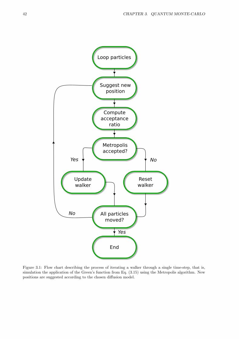
42 CHAPTER 3. QUANTUM MONTE-CARLO
Update walker
Reset walker
All particlesmoved?
End
Loop particles
Suggest newposition
Computeacceptance
ratio
Metropolisaccepted?
Yes No
No
Yes
Figure 3.1: Flow chart describing the process of iterating a walker through a single time-step, that is,simulation the application of the Green’s function from Eq. (3.15) using the Metropolis algorithm. Newpositions are suggested according to the chosen diffusion model.
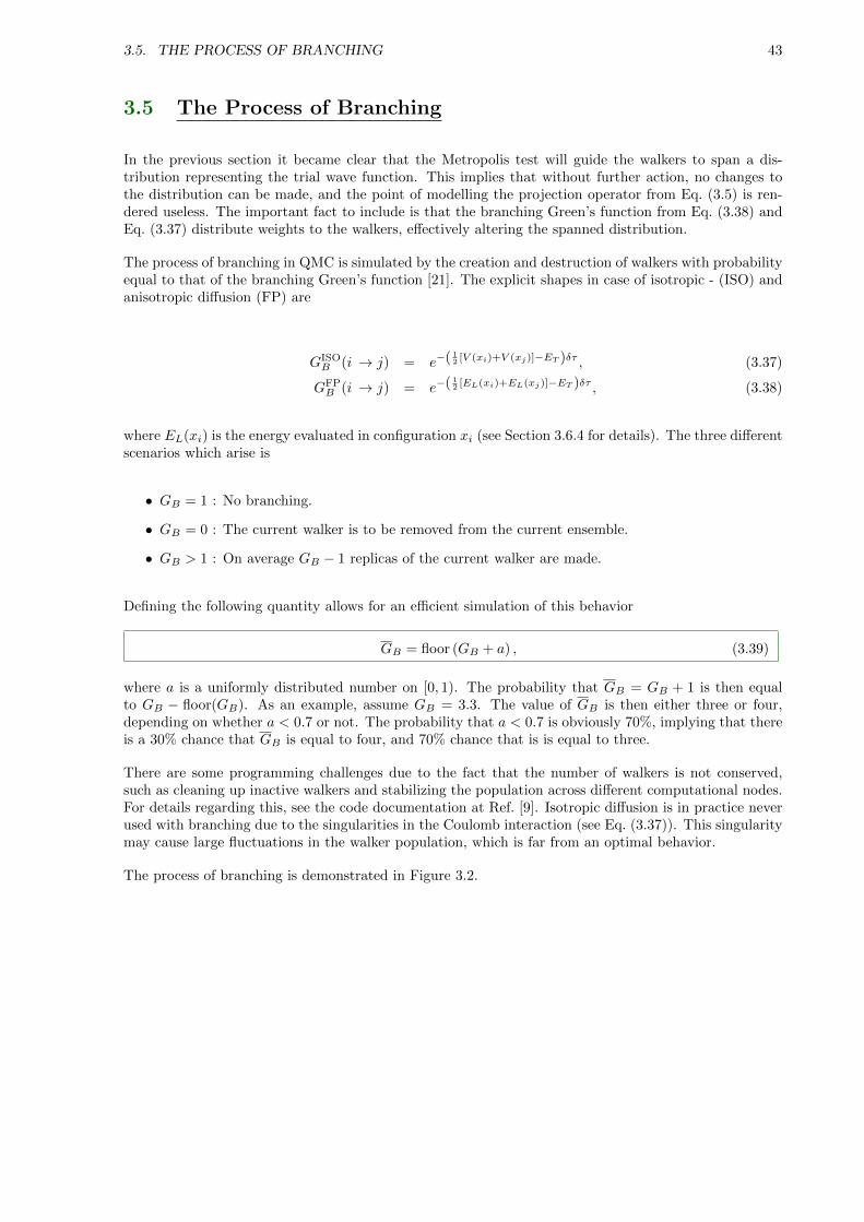
3.5. THE PROCESS OF BRANCHING 43
3.5 The Process of Branching
In the previous section it became clear that the Metropolis test will guide the walkers to span a dis-tribution representing the trial wave function. This implies that without further action, no changes tothe distribution can be made, and the point of modelling the projection operator from Eq. (3.5) is ren-dered useless. The important fact to include is that the branching Green’s function from Eq. (3.38) andEq. (3.37) distribute weights to the walkers, effectively altering the spanned distribution.
The process of branching in QMC is simulated by the creation and destruction of walkers with probabilityequal to that of the branching Green’s function [21]. The explicit shapes in case of isotropic - (ISO) andanisotropic diffusion (FP) are
GISOB (i → j) = e−( 1
2 [V (xi)+V (xj)]−ET )δτ , (3.37)
GFPB (i → j) = e−( 1
2 [EL(xi)+EL(xj)]−ET )δτ , (3.38)
where EL(xi) is the energy evaluated in configuration xi (see Section 3.6.4 for details). The three differentscenarios which arise is
• GB = 1 : No branching.
• GB = 0 : The current walker is to be removed from the current ensemble.
• GB > 1 : On average GB − 1 replicas of the current walker are made.
Defining the following quantity allows for an efficient simulation of this behavior
GB = floor (GB + a) , (3.39)
where a is a uniformly distributed number on [0, 1). The probability that GB = GB + 1 is then equalto GB − floor(GB). As an example, assume GB = 3.3. The value of GB is then either three or four,depending on whether a < 0.7 or not. The probability that a < 0.7 is obviously 70%, implying that thereis a 30% chance that GB is equal to four, and 70% chance that is is equal to three.
There are some programming challenges due to the fact that the number of walkers is not conserved,such as cleaning up inactive walkers and stabilizing the population across different computational nodes.For details regarding this, see the code documentation at Ref. [9]. Isotropic diffusion is in practice neverused with branching due to the singularities in the Coulomb interaction (see Eq. (3.37)). This singularitymay cause large fluctuations in the walker population, which is far from an optimal behavior.
The process of branching is demonstrated in Figure 3.2.
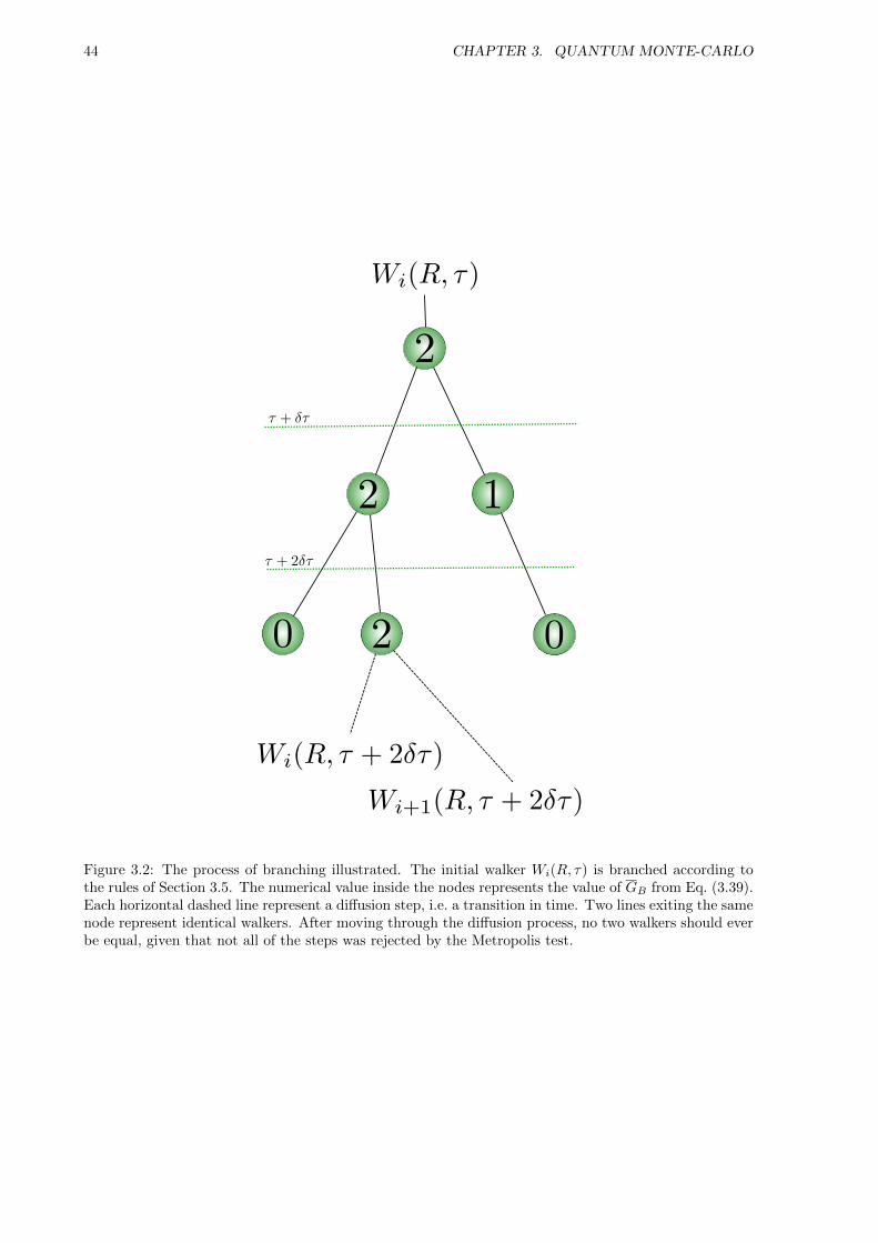
44 CHAPTER 3. QUANTUM MONTE-CARLO
Figure 3.2: The process of branching illustrated. The initial walker Wi(R, τ) is branched according tothe rules of Section 3.5. The numerical value inside the nodes represents the value of GB from Eq. (3.39).Each horizontal dashed line represent a diffusion step, i.e. a transition in time. Two lines exiting the samenode represent identical walkers. After moving through the diffusion process, no two walkers should everbe equal, given that not all of the steps was rejected by the Metropolis test.
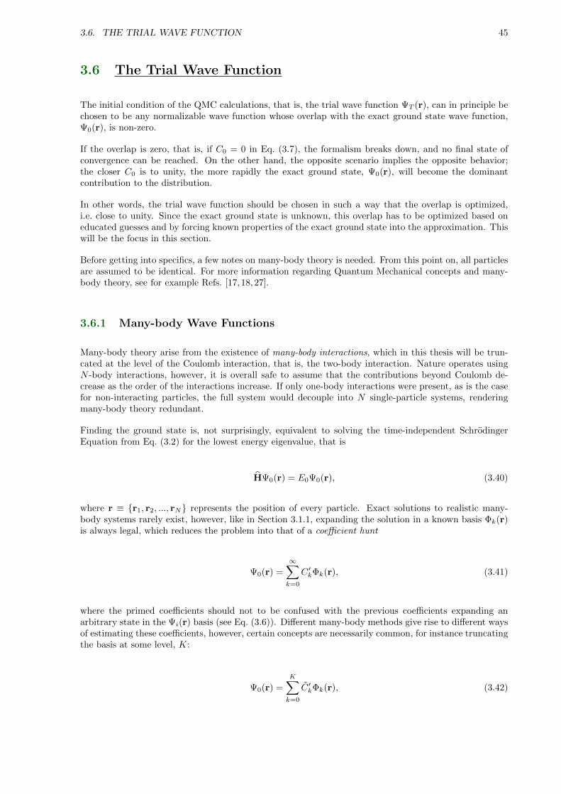
3.6. THE TRIAL WAVE FUNCTION 45
3.6 The Trial Wave Function
The initial condition of the QMC calculations, that is, the trial wave function ΨT (r), can in principle bechosen to be any normalizable wave function whose overlap with the exact ground state wave function,Ψ0(r), is non-zero.
If the overlap is zero, that is, if C0 = 0 in Eq. (3.7), the formalism breaks down, and no final state ofconvergence can be reached. On the other hand, the opposite scenario implies the opposite behavior;the closer C0 is to unity, the more rapidly the exact ground state, Ψ0(r), will become the dominantcontribution to the distribution.
In other words, the trial wave function should be chosen in such a way that the overlap is optimized,i.e. close to unity. Since the exact ground state is unknown, this overlap has to be optimized based oneducated guesses and by forcing known properties of the exact ground state into the approximation. Thiswill be the focus in this section.
Before getting into specifics, a few notes on many-body theory is needed. From this point on, all particlesare assumed to be identical. For more information regarding Quantum Mechanical concepts and many-body theory, see for example Refs. [17, 18,27].
3.6.1 Many-body Wave Functions
Many-body theory arise from the existence of many-body interactions, which in this thesis will be trun-cated at the level of the Coulomb interaction, that is, the two-body interaction. Nature operates usingN -body interactions, however, it is overall safe to assume that the contributions beyond Coulomb de-crease as the order of the interactions increase. If only one-body interactions were present, as is the casefor non-interacting particles, the full system would decouple into N single-particle systems, renderingmany-body theory redundant.
Finding the ground state is, not surprisingly, equivalent to solving the time-independent SchrodingerEquation from Eq. (3.2) for the lowest energy eigenvalue, that is
HΨ0(r) = E0Ψ0(r), (3.40)
where r ≡ {r1, r2, ..., rN} represents the position of every particle. Exact solutions to realistic many-body systems rarely exist, however, like in Section 3.1.1, expanding the solution in a known basis Φk(r)is always legal, which reduces the problem into that of a coefficient hunt
Ψ0(r) =
∞∑k=0
C ′kΦk(r), (3.41)
where the primed coefficients should not to be confused with the previous coefficients expanding anarbitrary state in the Ψi(r) basis (see Eq. (3.6)). Different many-body methods give rise to different waysof estimating these coefficients, however, certain concepts are necessarily common, for instance truncatingthe basis at some level, K:
Ψ0(r) =
K∑k=0
C ′kΦk(r), (3.42)
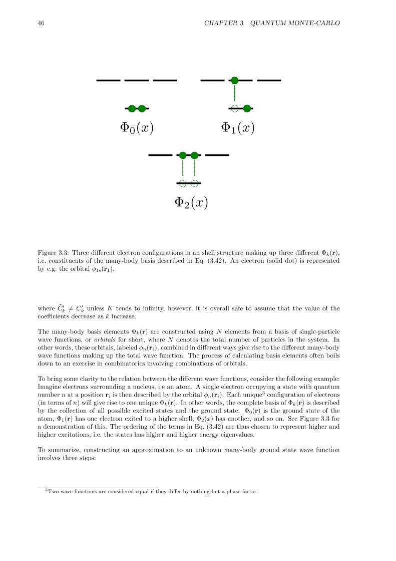
46 CHAPTER 3. QUANTUM MONTE-CARLO
Figure 3.3: Three different electron configurations in an shell structure making up three different Φk(r),i.e. constituents of the many-body basis described in Eq. (3.42). An electron (solid dot) is representedby e.g. the orbital φ1s(r1).
where C ′k 6= C ′k unless K tends to infinity, however, it is overall safe to assume that the value of thecoefficients decrease as k increase.
The many-body basis elements Φk(r) are constructed using N elements from a basis of single-particlewave functions, or orbitals for short, where N denotes the total number of particles in the system. Inother words, these orbitals, labeled φn(ri), combined in different ways give rise to the different many-bodywave functions making up the total wave function. The process of calculating basis elements often boilsdown to an exercise in combinatorics involving combinations of orbitals.
To bring some clarity to the relation between the different wave functions, consider the following example:Imagine electrons surrounding a nucleus, i.e an atom. A single electron occupying a state with quantumnumber n at a position ri is then described by the orbital φn(ri). Each unique3 configuration of electrons(in terms of n) will give rise to one unique Φk(r). In other words, the complete basis of Φk(r) is describedby the collection of all possible excited states and the ground state. Φ0(r) is the ground state of theatom, Φ1(r) has one electron exited to a higher shell, Φ2(x) has another, and so on. See Figure 3.3 fora demonstration of this. The ordering of the terms in Eq. (3.42) are thus chosen to represent higher andhigher excitations, i.e. the states has higher and higher energy eigenvalues.
To summarize, constructing an approximation to an unknown many-body ground state wave functioninvolves three steps:
3Two wave functions are considered equal if they differ by nothing but a phase factor.
3.6. THE TRIAL WAVE FUNCTION 47
Step one Choose a basis of orbitals φn(ri), e.g. hydrogen states.Step two Construct Φk(r) from N× φn(ri).Step three Construct Ψ0(r) from K× φk(r).
The last step is well described by Eq. (3.42), but is seldom necessary to perform explicitly; expressionsinvolving the approximated ground state wave function is given in terms of the constituent Φk(r) elementsand their coefficients.
Step one in detail
The Hamiltonian of an N -particle system is
H = H0 + HI, (3.43)
where H0 and HI are the one-body - and the many-body Hamiltonian, respectively. As mentioned in theintroduction, the many-body interactions are truncated at the level of the two-body Coulomb interaction.The one-body term consist of the external potential uext(ri) and the kinetic term t(ri) for all particles.In order words, the two Hamiltonians are written
H0 =
N∑i=1
h0(ri) (3.44)
=
N∑i=1
t(ri) + uext(ri),
and
HI 'N∑
i<j=1
v(rij) (3.45)
=
N∑i<j=1
1
rij,
where rij = |ri − rj | is the distance between two particles.
In order to optimize the overlap C0 with the exact wave function, the single-particle orbitals are commonlychosen to be the eigenfunctions of the non-interacting single-particle Hamiltonian, that is
h0(ri)φn(ri) = εnφn(ri). (3.46)
If no such choice can be made, choosing, free-particle solutions, Laguerre polynomials, or similar, is thegeneral strategy. However, for these bases, the expansion truncation K from Eq. (3.42) needs to be higherin order to achieve a satisfying overlap.
Step two in detail
In the case of fermions, that is, half-integer spin particles like electrons, protons, etc., Φk(r) is an anti-symmetric function4 on the form of a determinant: The so-called Slater determinant. The shape of the
4Interchanging two particles in an anti-symmetric wave function will reproduce the state changing only the sign.
48 CHAPTER 3. QUANTUM MONTE-CARLO
determinant is given in Eq. (3.47). The anti-symmetry is a direct consequence of the Pauli ExclusionPrinciple: At any given time, two fermions cannot occupy the same state.
Bosons, on the other hand, have symmetric wave functions, which in many ways are easier to deal withbecause of the lack of an exclusion principle. The bosonic many-body wave function is given in Eq. (3.48).In order to keep the terminology less abstract and confusing, the focus will be on systems of fermionsfrom here on.
ΦAS0 (r1, r2, ..., rN ) ∝
∑P
(−)PPφ1(r1)φ2(r2) ... φN (rN )
=
∣∣∣∣∣∣∣∣∣φ1(r1) φ2(r1) · · · φN (r1)φ1(r2) φ2(r2) · · · φN (r2)
......
. . ....
φ1(rN ) φ2(rN ) · · · φN (rN )
∣∣∣∣∣∣∣∣∣ , (3.47)
ΦS0(r1, r2, ..., rN ) ∝
∑P
Pφ1(r1)φ2(r2) ... φN (rN ). (3.48)
The permutation operator P is simply a way of writing in any combination of particles and states, hencethe combinatoric exercise mentioned previously. Any combination of N orbital elements φn(ri) can beused to produce different Φk(r). For illustrative purposes, and for the purpose of this thesis in generalwhere a single determinant ansatz is used, only the ground state has been presented.
Dealing with correlations
The contributions to the ground state on the right-hand side in Eq. (3.41) for k > 0 are referred to ascorrelation terms. Given that the single-particle wave functions are chosen by Eq. (3.46), the existenceof the correlation terms, i.e. C ′k 6= 0 for k > 0, follows as a direct consequence of the electron-electroninteraction, hence the name.
As an example, imagine performing an energy calculation with two particles being infinitely close; theCoulomb singularity will cause the energy to blow up. However, if the calculations are performed usingthe exact wave function, the diverging terms will cancel out; the energy eigenvalue is independent of theposition of the state.
In other words, a necessary property of the exact wave function is that the singularities in the many-body interactions are canceled. The basic idea is thus to make sure the trial wave function also has thisproperty. By doing so, it is brought closer to the exact wave function.
These criteria are called cusp conditions [26], and serve as powerful guides when it comes to selecting anoptimal trial wave function.
3.6.2 Choosing the Trial Wave Function
To recap, choosing the trial wave function boils down to optimizing the overlap C0 = 〈Ψ0|ΨT 〉 using apriori knowledge about the system at hand. As discussed previously, the optimal choice of single-particlebasis is the eigenfunctions of the non-interacting case (given that they exist). Starting from Eq. (3.42),from here on referred to as the spatial wave function, the first step is to make sure the cusp conditionsare obeyed.
3.6. THE TRIAL WAVE FUNCTION 49
Introducing the correlation functions f(rij), where rij is the relative distance between particle i and j,the general ansatz for the trial wave function becomes
ΨT (r1, ..., rN ) =[ K∑k=0
CkΦk(r1, ..., rN )] N∏i<j
f(rij). (3.49)
The idea is now to choose f(rij) in such a way that the cusp conditions are obeyed. This should, inlight of previous discussions, reduce the amount of terms needed in the spatial wave function to obtain asatisfying overlap.
Explicit shapes
Several models for the correlation function exist, however, some are less practical than others. An examplegiven in ref. [21] demonstrates this nicely: Hylleraas presented the following correlation function
f(rij)Hylleraas = e−12 (ri+rj)
∑k
dk(rij)ak(ri + rj)
bk(ri − rj)ek , (3.50)
where all k-subscripted parameters are free. Calculating the helium ground state energy using thiscorrelation function with nine terms yields a four decimal precision. Eight digit precision is achieved byincluding 1078 terms. For the purpose of QMC, including such vast amounts of parameters is out of thequestion. The strength of QMC is that very good results can be obtained using a very simple ansatz tothe wave function.
A commonly used correlation function in studies involving few variational parameters is the Pade Jastrowfunction
N∏i<j
f(rij) = exp(U),
U =
N∑i<j
( ∑k akr
kij
1 +∑k βkr
kij
)+
N∑i
( ∑k a′krki
1 +∑k αkr
ki
).
For systems where the correlations are relatively well behaved, it is custom to drop the second sum alltogether, and keep only the k = 1 term from the first. The resulting function reads
f(rij ;β) = exp
(aijrij
1 + βrij
), (3.51)
where β is a variational parameter, and ak=1 ≡ aij is a constant depending on the relative spin-orientationof particles i and j tuned in such a way that the cusp conditions are obeyed. For three dimensions,aij = 1/4 or aij = 1/2 depending on whether or not the spins of i and j are parallell or anti parallell,respectively [21]. For two dimensions, the values are aij = 1/3 (parallell) or aij = 1 (anti-parallel) [28].This is the correlation function used for all systems in this thesis.
Shifting the focus back to the spatial wave function, in the case of a fermionic system, the evaluation of anN ×N Slater determinant severely limits the efficiency of many-particle simulations. However, assumingthe Hamiltonian to be spin-independent, the eigenstates for different spin eigenvalues will be identical.
50 CHAPTER 3. QUANTUM MONTE-CARLO
This fact results in the spatial wave function being split in two: One part for each spin eigenvalue. Adetailed derivation of this is given in the appendix of Ref. [29]. The resulting wave function thus becomes
ΨT (r;β) =[ K∑k=0
C ′kΦk(r1, ..., rN2
)Φk(rN2 −1, ..., rN )
] N∏i<j
f(rij ;β). (3.52)
Due to the identical nature of the particles, they may be arbitrarily ordered. For simplicity, the first halfrepresents spin up, and the second half spin down. The spin up determinant will from here on be labeled|S↑|, and the spin down one |S↓|, where the S matrix will be referred to as the Slater matrix. Stitchingeverything together, the explicit shape of the trial wave function becomes
ΨT (r1, ..., rN ;β) =
K∑k=0
C ′k|S↑|k|S↓|kN∏i<j
f(rij ;β). (3.53)
This shape is referred to as a multi-determinant trial wave function unless K = 1, in which it will bereferred to as a single-determinant trial wave function.
Limitations
Depending on the complexity of the system at hand, more complicated trial wave functions might beneeded to obtain reasonable convergence. However, it is important to distinguish between simply in-tegrating a trial wave function, and performing the full diffusion calculation. As a reminder: Simpleintegration will not be able to alter the distribution; what you have is what you get. Solving the diffusionproblem, on the other hand, will alter the distribution from that of the trial wave function (τ = 0) intoa distribution closer to the exact wave function by Eq. (3.6).
Because of this fact, limitations due to the trial wave function in full5 QMC is far less than what isthe case of standard Monte-Carlo integration. A more complex trial wave function might convergencefaster, but at the expense of being more CPU-intensive. This implies that CPU time per walker can betraded for convergence time. For systems of many particles, the CPU time per walker needs to be as lowas possible in order to get the computation done in a reasonable amount of time. In other words, thechoice of trial wave function needs to be done in light of the system at hand, and the specific aim of thecomputation.
On the other hand, when the number of particles in the system increase, it is safe to assume that thequality of the trial wave function will decrease. This is demonstrated in Ref. [30], where calculationsfor F2 (18 particles) need an increase in the number of determinants to achieve a result with the sameprecision as calculations for O2 (16 particles).
Single-determinant trial wave functions
In the case of well-behaving systems, a single determinant with a simple Jastrow factor serves as areasonable trial wave function. This simplicity opens up the possibility of simulating large systemsefficiently. More details regarding this will be given in Section 4.3.
In order to further optimize the overlap with the exact wave function, a second variational parameter αis introduced in the spatial wave function
5“Full” in the sense that all Green’s functions are applied. As will be revealed later, VMC corresponds to a standardimportance sampled Monte-Carlo integration by omitting the branching process.
3.6. THE TRIAL WAVE FUNCTION 51
ΨT (r1, ..., rN ;α, β) = D↑(α)D↓(α)
N∏i<j
f(rij ;β). (3.54)
Determining the optimal values of the variational parameters will be the topic of the next section. If theintroduction of the variational parameter was redundant, optimizations would simply yield α = 1.
3.6.3 Selecting Optimal Variational Parameters
All practical ways of determining the optimal values of the variational parameters originate from thesame powerful principle: The Variational Principle. The easiest way of demonstrating the principle isto evaluate the expectation value of the energy, using an approach similar to what used in Eq. (3.6).Consider the following relations
Ek = 〈Ψk| H |Ψk〉 ,E = 〈ΨT (α, β)| H |ΨT (α, β)〉
=∑kl
C∗kCl 〈Ψk| H |Ψl〉︸ ︷︷ ︸Ekδkl
=∑k
|Ck|2Ek.
Just as with the projection operator, introducing Ek = E0 + δEk where δEk ≥ 0 will simplify thearguments
E =∑k
|C2k |(E0 + δEk)
= E0
∑k
|C2k |︸ ︷︷ ︸
1
+∑k
|Ck|2δEk︸ ︷︷ ︸≥0
≥ E0.
The conclusion is remarkable: No matter which trial wave function is used, the resulting energy willalways be greater or equal to the exact ground state energy. This implies that the problem of choosingvariational parameters comes down to a minimization problem in the parameters space
∂〈E〉∂αi
=∂
∂αi〈ΨT (αi)| H |ΨT (αi)〉 = 0 (3.55)
In order to work with Eq. (3.55) in practice, it needs to be rewritten in terms of known values. Sincethe wave function depends on the variational parameter, the normalization factor needs to be includedin the expression of the expectation value. Applying the product rule numerous times yields
52 CHAPTER 3. QUANTUM MONTE-CARLO
∂〈E〉∂αi
=∂
∂αi
〈ΨT (αi)| H |ΨT (αi)〉〈ΨT (αi)|ΨT (αi)〉
=
(〈ΨT (αi)| ∂
∂αiH |ΨT (αi)〉+ 〈ΨT (αi)| H ∂
∂αi|ΨT (αi)〉
)〈ΨT (αi)|ΨT (αi)〉2
〈ΨT (αi)|ΨT (αi)〉
− 〈ΨT (αi)| H |ΨT (αi)〉
(〈ΨT (αi)| ∂
∂αi
)|ΨT (αi)〉+ 〈ΨT (αi)|
(∂∂αi|ΨT (αi)〉
)〈ΨT (αi)|ΨT (αi)〉2
.
The Hamiltonian does not depend on the variational parameters, hence both terms in the first expansionis equal. Cleaning up the expression yields
∂〈E〉∂αi
= 2
(〈ΨT (αi)| H ∂
∂αi|ΨT (αi)〉
〈ΨT (αi)|ΨT (αi)〉− 〈E〉
〈ΨT (αi)| ∂∂αi|ΨT (αi)〉
〈ΨT (αi)|ΨT (αi)〉
)
= 2
(⟨E∂ΨT
∂αi
⟩− 〈E〉
⟨∂ΨT
∂αi
⟩). (3.56)
In the case of ΨT (r;αi) being represented by a Slater determinant, the relationship between the variationalderivative of the determinant and the variational derivative of the single-particle orbitals φn(ri;αi) is
∂ΨT (r;αi)
∂αi=
N∑p=1
N/2∑q=0
φq(rp;αi)
[∂φq(rp;αi)
∂αi
]S−1qp , (3.57)
where S−1qi is the inverse of the Slater matrix, which will be discussed in more detail in Section 4.4.1.
Using these expressions for the variational energy gradient, the derivatives can be calculated exactly thesame way the energy. The gradient can then be used to move in the direction of the variational minimumin Eq. (3.55).
This strategy gives rise to numerous ways of finding the optimal parameters, such as using the well knownNewton’s method, conjugate gradient methods [31], steepest descent (similar to Newton’s method), andmany more. The method implemented for this thesis is called Adaptive Stochastic Gradient Descent, andis an efficient iterative algorithm for seeking the variational minimum. The gradient descent methodswill be covered in Section 3.7.
3.6.4 Calculating Expectation Values
The expectation value of an operator O is obtained by sampling local values, OL(x)
3.6. THE TRIAL WAVE FUNCTION 53
〈ΨT | O |ΨT 〉 =
∫ΨT (x)∗OΨT (x)dx
=
∫|ΨT |2
(1
ΨT (x)OΨT (x)
)dx
=
∫|ΨT |2OL(x)dx. (3.58)
OL(x) =1
ΨT (x)OΨT (x). (3.59)
Discretizing the integral yields
〈ΨT | O |ΨT 〉 ≡ 〈O〉 '1
n
n∑i=1
OL(xi) ≡ O, (3.60)
where xi is a random variable taken from distribution of the trial wave function. The ensemble average,〈O〉 will, given ergodicity, equal the estimated average O in the limit n→∞, that is
〈O〉 = limn→∞
O = limn→∞
1
n
n∑i=1
OL(xi). (3.61)
In the case of the energy estimation, this implies that once the walkers reach equilibrium, local values canbe sampled based on their configurations ri (remember that Metropolis ensures that the walkers follow|ΨT (r)|2). In the case of energies, the explicit expression becomes
〈E〉 ' 1
n
n∑i=1
(1
ΨT (ri)
(−1
2∇2
)ΨT (ri) + V (ri)
). (3.62)
Incorporating the branching Green’s function GB into the above equation is covered in the DMC section.
3.6.5 Normalization
Every explicit calculation using the trial wave function in QMC involves taking ratios. Calculating ratiosimplies a cancellation in the normalization factors. Eq. (3.32) from the Metropolis section, the quantumforce in the Fokker-Planck equation, and the sampling of local values described in the previous sectiondemonstrate exactly this; everything involves ratios.
Not having to normalize the wave functions does not only save a lot of CPU time, but it also removes theneed of including the normalization factors of the single-particle wave functions; any constants multiplyingφn(xi) in Eq. (3.47) and Eq. (3.48) can be taken outside the sum over permutations, and will thus cancelwhen the ratio between two wave functions constituting of the same single-particle orbitals are computed.
Note, however, that this argument is valid for single determinant wave functions only.

54 CHAPTER 3. QUANTUM MONTE-CARLO
Figure 3.4: Two steps of a one dimensional Gradient Descent process. Steps are taken in the directionof the negative gradient (indicated by dotted lines).
3.7 Gradient Descent Methods
The direction of a gradient serves as a guide to extremal values. Gradient descent, also called steepestdescent6, is a family of minimization methods using this property of gradients in order to backtrace alocal minimum in the vicinity of an initial guess.
3.7.1 General Gradient Descent
Seeking maxima or minima is simply a question of whether the positive or the negative direction of thegradient is followed. Imagine a function f(x), with a minimum residing at x = xm. The information athand is then
∇f(xm) = 0 (3.63)
∇f(xm − dx) < 0 (3.64)
∇f(xm + dx) > 0 (3.65)
where dx is a infinite decimal displacement.
As an example, imagine starting from an initial guess x0. The direction of the gradient is then calculatedand followed a number of steps. From Figure 3.4 and the previous equations, it is clear that crossing thetrue minimum induces a sign change in the gradient. The brute force way of minimizing is to simply endthe calculation at this point, however, this would require an extreme amount of very small steps in orderto achieve good precision.
The difference equation describing the steps from the previous paragraph is
xi+1 = xi − δ∇f(xi)
|∇f(xi)|. (3.66)
6In literature, steepest - and gradient descent are sometimes referred to as being different. However, for simplicity, thesewill not be differentiated.
3.7. GRADIENT DESCENT METHODS 55
An improved algorithm would be to continue iterating even though the minimum is crossed, however,this would cause the constant step-length algorithms to oscillate between two points, e.g. x1 and x2 inFigure 3.4. To counter this, a changing step-length δi is introduced
xi+1 = xi − δi∇f(xi). (3.67)
All gradient/steepest descent methods are in principle described by Eq. (3.67)7. Some examples are
•Brute Force I δi = δ 1|∇f(xi)|
•Brute Force II δi = δ
•Monotone Decreasing δi = δ/iN
•Newton’s Method δi = 1∇2f(xi)
Iterative gradient methods will only reveal one local extrema, depending on the choice of x0 and δ.In order to find several extrema, multiple unique processes can be run sequentially or in parallel withdifferent initial guesses.
3.7.2 Stochastic Gradient Descent
Minimizing stochastic quantities such as the variance and expectation values adds another layer of com-plications on top of the methods introduced in the previous section. Assuming a closed form expressionfor the stochastic quantity is unobtainable, the gradient needs to be calculated by using e.g. Monte-Carlosampling. Eq. (3.56) is an example of such a process.
A precise sampling of the stochastic quantities is expensive and unpractical. Stochastic gradient meth-ods use different techniques in order to make the sampling more effective, such as multiple walkers,thermalization, and more.
Using a finite difference scheme with stochastic quantities is dangerous, as uncertainties in the valueswill cause the gradient to become unstable when the variations are low close to the minimum. This isillustrated in Figure 3.5.
3.7.3 Adaptive Stochastic Gradient Descent
Adaptive Stochastic Gradient Descent (ASGD) has its roots in the mathematics of automated controltheory [32]. The automated process is that of choosing an optimal step-length δi for the current transitionxi → xi+1. This process is based on the inner product of the old and the new gradient though a variableXi
Xi ≡ −∇i · ∇i−1. (3.68)
The step-length from Eq. (3.67) is modelled in the following manner in ASGD:
7This fact sets the perfect scene for an object oriented implementation of gradient descent methods.
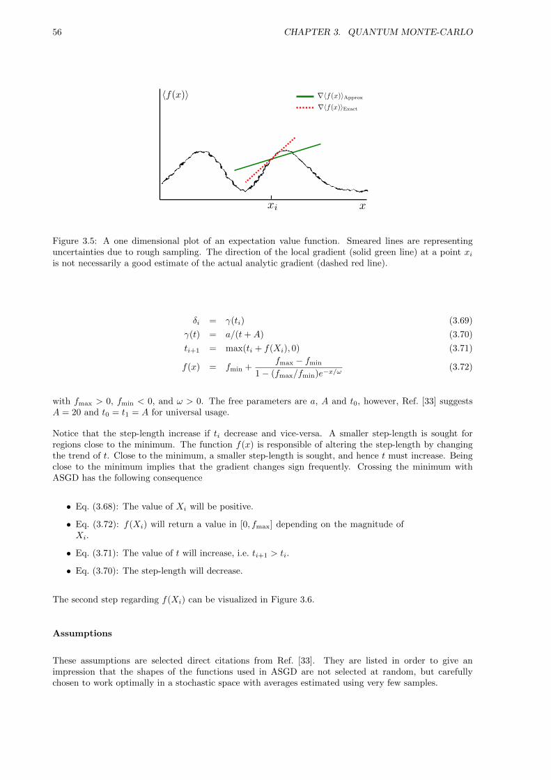
56 CHAPTER 3. QUANTUM MONTE-CARLO
Figure 3.5: A one dimensional plot of an expectation value function. Smeared lines are representinguncertainties due to rough sampling. The direction of the local gradient (solid green line) at a point xiis not necessarily a good estimate of the actual analytic gradient (dashed red line).
δi = γ(ti) (3.69)
γ(t) = a/(t+A) (3.70)
ti+1 = max(ti + f(Xi), 0) (3.71)
f(x) = fmin +fmax − fmin
1− (fmax/fmin)e−x/ω(3.72)
with fmax > 0, fmin < 0, and ω > 0. The free parameters are a, A and t0, however, Ref. [33] suggestsA = 20 and t0 = t1 = A for universal usage.
Notice that the step-length increase if ti decrease and vice-versa. A smaller step-length is sought forregions close to the minimum. The function f(x) is responsible of altering the step-length by changingthe trend of t. Close to the minimum, a smaller step-length is sought, and hence t must increase. Beingclose to the minimum implies that the gradient changes sign frequently. Crossing the minimum withASGD has the following consequence
• Eq. (3.68): The value of Xi will be positive.
• Eq. (3.72): f(Xi) will return a value in [0, fmax] depending on the magnitude ofXi.
• Eq. (3.71): The value of t will increase, i.e. ti+1 > ti.
• Eq. (3.70): The step-length will decrease.
The second step regarding f(Xi) can be visualized in Figure 3.6.
Assumptions
These assumptions are selected direct citations from Ref. [33]. They are listed in order to give animpression that the shapes of the functions used in ASGD are not selected at random, but carefullychosen to work optimally in a stochastic space with averages estimated using very few samples.

3.7. GRADIENT DESCENT METHODS 57
Figure 3.6: Examples of f(Xi) as published in Ref. [33]. As ω → 0, f(x) approaches a step function.
• The statistical error in the sampled gradients are distributed with zero mean.
This is shown in Ref. [33]; they are normally distributed. The implication is that upon combining gradientestimates for N different processes, the accumulative error will tend to zero quickly.
• The step-length γ(t) is a positive monotone decreasing function defined on [0,∞)with maximum at t = 0.
With γ(t) being as in Eq (3.70), this is easily shown.
• The function f(x) is continuous and monotone increasing with fmin = limx→∞
f(x)
and fmax = limx→−∞
f(x).
This is exactly the behavior displayed in Figure 3.6.
Implementation
A flow chart of the implementation is given in Figure 3.8. For specific details regarding the implementa-tion, see the documentation of the code in Ref. [9]. An example of minimization using ASGD is given inFigure 3.7.

58 CHAPTER 3. QUANTUM MONTE-CARLO
Figure 3.7: Results of Adaptive Stochastic Gradient Descent used on a two-particle quantum dot with unitoscillator frequency using 400 cycles pr. gradient sampling and 40 independent walkers. The right figureshows the evolution of the time-step. The left figure shows the evolution of the variational parameters αand β introduced in Section 3.6 on top, and the evolution of the gradients on the bottom. The gradientsare averaged to reveal the pattern underlying the noise. Dispite this averaging, it is apparent that theytend to zero, β somewhat before α. The step rushes to zero with a small rebound as it attempts to crossto negative values.
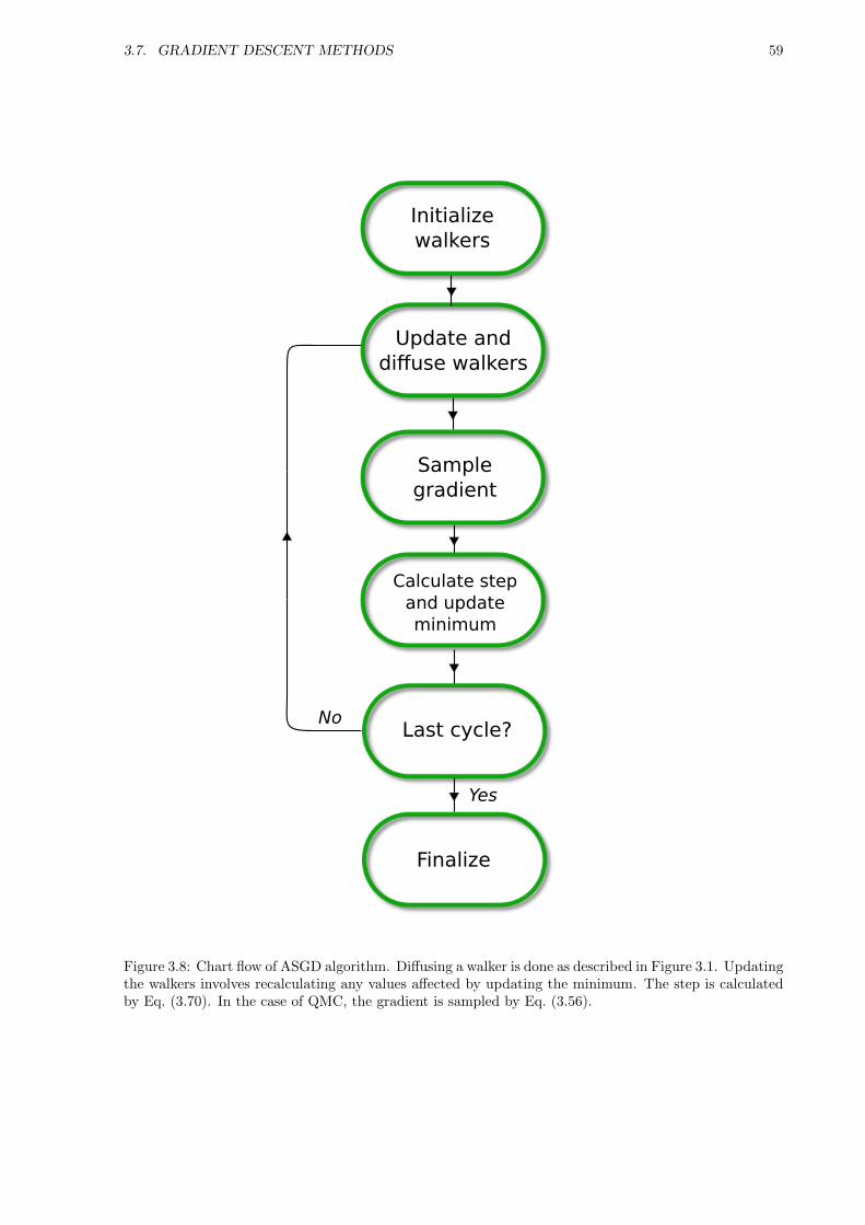
3.7. GRADIENT DESCENT METHODS 59
Finalize
Initializewalkers
Update anddiffuse walkers
Samplegradient
Last cycle?
Calculate stepand update minimum
Yes
No
Figure 3.8: Chart flow of ASGD algorithm. Diffusing a walker is done as described in Figure 3.1. Updatingthe walkers involves recalculating any values affected by updating the minimum. The step is calculatedby Eq. (3.70). In the case of QMC, the gradient is sampled by Eq. (3.56).
60 CHAPTER 3. QUANTUM MONTE-CARLO
3.8 Variational Monte-Carlo
As briefly mentioned in the Section 3.1.1, neglecting the branching term, i.e. setting GB = 1, correspondsto a method called Variational Monte-Carlo (VMC). The name comes from the fact that the method isis variational, that is, it supplies an upper bound to the exact ground state energy. The better the trialwave function is, the closer the VMC energy is to the exact ground state energy.
The converged state of the Markov chain in VMC is controlled by the Metropolis test, and will thus equalthe trial wave function squared. From the flow chart of the VMC algorithm in Figure 3.9, it is clear thatVMC corresponds to a standard Monte-Carlo integration of the local energy sampled using a distributionequal to the trial wave function squared.
3.8.1 Motivating the use of Diffusion Theory
An important question to answer is why e.g. the Langevin equation is so important if the result is simplyan expectation value. Statistics states that any distribution may be used when calculating an expectationvalue. Why bother with a trial wave function, thermalization, and so on?
The reason is simple, yet not obvious. The quantity of interest, the local energy, depends on the trialwave function. This is demonstrated in the following expression:
EVMC =
∫P (r)
1
ΨT (r)HΨT (r)dr
' 1
n
n∑i=1
1
ΨT (ri)HΨT (ri), (3.73)
where the points ri are drawn from the distribution P (r).
Equation (3.73) implies that the evaluation of the local energy in an arbitrary distribution P (r) isundefined at the zeros of ΨT (r). In other words, it is not guaranteed that P (r) does not generate apoint rm in such a way that ΨT (rm) = 0.
However, if the distribution is chosen as P (r) = |ΨT (r)|2, the probability of sampling a point where thelocal energy is undefined equals zero. This comes as a consequence of the following relation
ΨT (rm) = 0 =⇒ P (rm) = 0 (3.74)
In other words, the more undefined the energy is at a point, the less probable the point is. This hiddendetail is what Quantum Monte-Carlo safely takes care of that standard Monte-Carlo does not.
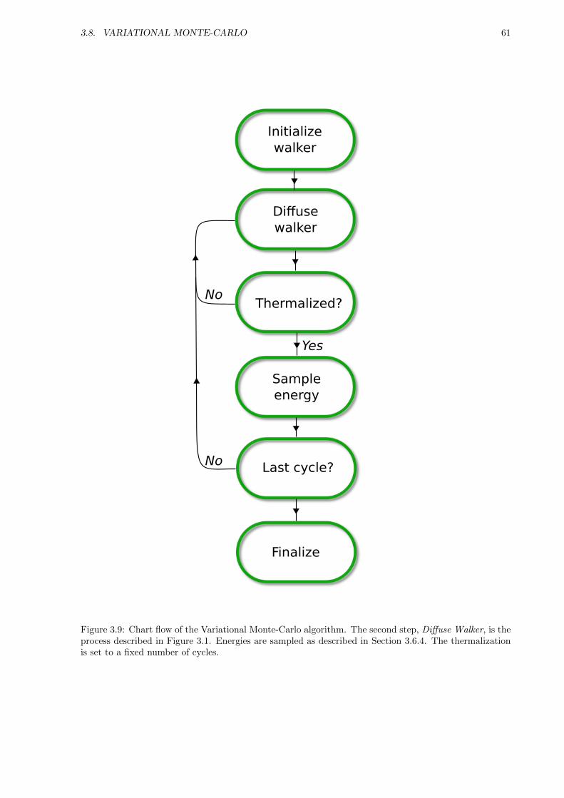
3.8. VARIATIONAL MONTE-CARLO 61
Finalize
Yes
Initializewalker
Diffuse walker
Thermalized?
Sampleenergy
Last cycle?
No
No
Figure 3.9: Chart flow of the Variational Monte-Carlo algorithm. The second step, Diffuse Walker, is theprocess described in Figure 3.1. Energies are sampled as described in Section 3.6.4. The thermalizationis set to a fixed number of cycles.
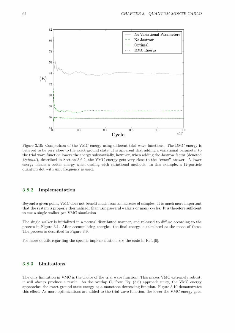
62 CHAPTER 3. QUANTUM MONTE-CARLO
Figure 3.10: Comparison of the VMC energy using different trial wave functions. The DMC energy isbelieved to be very close to the exact ground state. It is apparent that adding a variational parameter tothe trial wave function lowers the energy substantially, however, when adding the Jastrow factor (denotedOptimal), described in Section 3.6.2, the VMC energy gets very close to the “exact” answer. A lowerenergy means a better energy when dealing with variational methods. In this example, a 12-particlequantum dot with unit frequency is used.
3.8.2 Implementation
Beyond a given point, VMC does not benefit much from an increase of samples. It is much more importantthat the system is properly thermalized, than using several walkers or many cycles. It is therefore sufficientto use a single walker per VMC simulation.
The single walker is initialized in a normal distributed manner, and released to diffuse according to theprocess in Figure 3.1. After accumulating energies, the final energy is calculated as the mean of these.The process is described in Figure 3.9.
For more details regarding the specific implementation, see the code in Ref. [9].
3.8.3 Limitations
The only limitation in VMC is the choice of the trial wave function. This makes VMC extremely robust;it will always produce a result. As the overlap C0 from Eq. (3.6) approach unity, the VMC energyapproaches the exact ground state energy as a monotone decreasing function. Figure 3.10 demonstratesthis effect. As more optimizations are added to the trial wave function, the lower the VMC energy gets.
3.9. DIFFUSION MONTE-CARLO 63
3.9 Diffusion Monte-Carlo
Applying the full diffusion framework introduced in Sections 3.1.1 and 3.2 results in a method knownas Diffusion Monte-Carlo (DMC)8. Diffusion Monte-Carlo results are often referred to as exact, in thesense that DMC is overall one of the most precise many-body methods available. However, just as anymany-body method, DMC also has its limitations. These will be discussed in Section 3.9.3.
Where other many-body methods run into the curse of dimensionality, that is, the run time scales verybad with increasing number of particles, DMC with its position basis Quantum Monte-Carlo formalismdoes not. With DMC, it is simply a matter of evaluating a more complicated trial wave function, orsimulating for a longer period of cycles, in order to reach convergence to the believed “exact” groundstate in a satisfactory way.
3.9.1 Implementation
Branching is a major part of the DMC algorithm. Diffusion Monte-Carlo uses a large ensemble of walkersto generate enormous amounts of statistics. These walkers are initialized using a VMC calculation, i.e. thewalkers are initially distributed according to the trial wave function squared.
There are three layers of loops in the DMC method implemented in this thesis, two of which are obvious:The time-step - and walker loops. However, introducing a third block loop within the walker loop booststhe convergence dramatically. For each walker, this loop continues until the walker is either dead (GB =0), or has diffused nb times. Using this method, “good” walkers will have multiple offspring pr cycle,while “bad” walkers will rarely survive the block loop. Perfect walkers will supply a ton of statistics asthey surf through all the loops without branching (GB ∼ 1).
A flow chart of the DMC algorithm is given in Figure 3.11. Comparing it the the corresponding figurefor VMC, it is apparent that DMC is by far more complicated.
3.9.2 Sampling the Energy
As mentioned in Section 3.1.1, the role of the branching Green’s function is to distribute the correctweights to each walker. Each walker’s contribution to the cumulative energy sampling should thus beweighed according to the value of the branching Green’s function. Let Ek denote the cumulative energyfor time-step τ = kδτ , nw be the number of walkers in the system at time-step k, nb,i be the number ofblocks walker i survives, and let Wi(r, τ) represent walker i. The relation is then
Ek =1
nw
nw∑i=1
1
nb,i
nb,i∑l=1
GB
(Wi(r, τk + lδτ)
)EL
(Wi(r, τk + lδτ)
). (3.75)
As required, setting GB = nw = nb = 1 reproduces the VMC expression.
The new trial energy from Eq. (3.13) is set equal to the previous cycle’s average energy, that is
ET = Ek. (3.76)
The DMC energy is updated each cycle to be the trailing average of the trial energies:
8In literature, DMC is also known as Projection Monte-Carlo, for reasons described in Section 3.1.1.
64 CHAPTER 3. QUANTUM MONTE-CARLO
EDMC = ET =1
n
n∑k=1
Ek. (3.77)
3.9.3 Limitations
By introducing the branching term, DMC is a far less robust method compared to VMC. Action must betaken in order to stabilize the iterations through tuning of parameters such as population size, time-step,block size, etc. This is the disadvantage of DMC compared to other many-body methods such as CoupledCluster [2], which is far more automatic.
Time-step errors
The error introduced by the short time approximation in Eq. (3.14) goes as O(δτ2). In addition, thereis a second error related to the time-step, arising from the fact that not all steps are accepted by theMetropolis algorithm. This introduces a effective reduction in the time-step, and is countered by scalingthe time-step with the acceptance ratio upon calculating GB [21]. However, DMC is rarely used withoutimportance sampling, which, due to the quantum force, has an acceptance ratio very close to one. It istherefore common to ignore this problem, as its effect on the final result is minimal.
Selecting the time-step
Studying the branching Green’s function in equation 3.38 in more detail reveals that it’s magnitudeincreases exponentially with the spread of the energies ∆E, that is
GB ∝ exp (∆Eδτ). (3.78)
As will be shown in Section 3.11.1, the spread in energy samples are higher the worse of an approximationto the ground state the trial wave function is. In addition, the magnitude of the spread scales with themagnitude of the energy.
Setting an upper bound to the branching function might seem like a good idea, however, each time awalker is denied its replicas, an uncontrollable error is introduced in the distribution.
The solution is to balance out the increase in ∆E by lowering the time-step accordingly. That is
δτ ∝ 1
∆E. (3.79)
However, having too low a time-step will hinder DMC from evolving walkers efficiently, especially if thepositional span of the distribution is large. In other words, a balance must be found. An indication ofwhether the time-step was chosen too low or not is obtained by looking at the resulting DMC density. Ifthe density is spiky and disorganized, the time-step was too low.
Another source of error is due to the fixed node approximation. This approximation will be covered inthe next section.

3.9. DIFFUSION MONTE-CARLO 65
Last DMC cycle?
Initializewalkers
Diffuse and Branch walker i
Sample energies
Current walkerdead or lastblock cycle?
Last walker?
Finalize
i = 0
i = 0
Clean-up i++
Yes
Yes
Yes
No
No
No
Figure 3.11: Chart flow of the Diffusion Monte-Carlo algorithm. The variable i represents the currentlymoved walker. The second step, Diffuse and Branch Walker, is the process described in Figure 3.1 incombination with the branching from Figure 3.2. Energies are sampled as in Eq. (3.75). Thermalizationis set to a fixed number of cycles.

66 CHAPTER 3. QUANTUM MONTE-CARLO
3.9.4 Fixed node approximation
Looking at Eq. (3.48), it is apparent that by choosing positive phases for the single-particle wave functions,the bosonic many-body wave function is exclusively positive. For fermions however, the sign change uponinterchanging two particles introduces the possibility that the wave function will have both negative andpositive regions, independent of the choice of phases in the single-particle wave functions.
As DMC iterates, the density of walkers at a given time, P (r, τ), represents the projected wave functionfrom Eq. (3.6) multiplied by the trial wave function.
P (r, τ) = Φ(r, τ)ΨT (r). (3.80)
This relationship is described in high detail in Section 3.2.2.
Applying the projector operator to the distribution yields
limτ→∞
P (r, τ) = 〈Φ0|ΦT 〉Φ0(r)ΨT (r), (3.81)
which, if interpreted as a density, should always be greater than zero. In the case of fermions, this is notguaranteed, as the node structure of the exact ground state and the trial wave function will generally bedifferent.
To avoid this anomaly in the density, Φ(r, τ) and ΨT (r) have to change sign simultaneously9. The bruteforce way of solving this problem is to fix the nodes by rejecting a walker’s step if the trial wave functionchanges sign:
ΨT (ri)
ΨT (rj)< 0 =⇒ A(i → j) = 0, (3.82)
where A(i → j) is the probability of accepting the move, as described in Section 3.4. An illustrativeexample is given in Figure 3.12.
3.10 Estimating One-body Densities
The one-body density is defined as
ρ(r1) =
∫∫r2r3
...
∫rN
|Φ(r1r2...rN )|2 dr2...drN . (3.83)
Unlike the distribution |Φ(r)|2, which describes the distribution of any of the particles in the system, theone-body density ρ(r1) describes the simultaneous distribution of every particle in the system, that is,ρ(r1)dr1 represents the probability of finding any of the system’s N particles within the volume elementdr1. Due to the indistinguishable nature of the particles, the fact that the first coordinate is chosen ispurely conventional; any of the N coordinates contain information about all the particles. For the samereason, the one-body density should be normalized to the number of particles, and not to unity.
9It should be mentioned that more sophisticated methods exist for dealing with the sign problem, some of which splitsthe distribution of walkers into a negative and a positive regions, however, due to the position space being infinite, thisrequires an enormous amount of walkers to succeed.
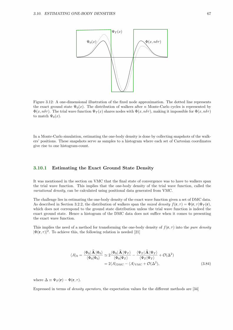
3.10. ESTIMATING ONE-BODY DENSITIES 67
Figure 3.12: A one-dimensional illustration of the fixed node approximation. The dotted line representsthe exact ground state Ψ0(x). The distribution of walkers after n Monte-Carlo cycles is represented byΦ(x, nδτ). The trial wave function ΨT (x) shares nodes with Φ(x, nδτ), making it impossible for Φ(x, nδτ)to match Ψ0(x).
In a Monte-Carlo simulation, estimating the one-body density is done by collecting snapshots of the walk-ers’ positions. These snapshots serve as samples to a histogram where each set of Cartesian coordinatesgive rise to one histogram-count.
3.10.1 Estimating the Exact Ground State Density
It was mentioned in the section on VMC that the final state of convergence was to have to walkers spanthe trial wave function. This implies that the one-body density of the trial wave function, called thevariational density, can be calculated using positional data generated from VMC.
The challenge lies in estimating the one-body density of the exact wave function given a set of DMC data.As described in Section 3.2.2, the distribution of walkers span the mixed density f(r, τ) = Φ(r, τ)ΨT (r),which does not correspond to the ground state distribution unless the trial wave function is indeed theexact ground state. Hence a histogram of the DMC data does not suffice when it comes to presentingthe exact wave function.
This implies the need of a method for transforming the one-body density of f(r, τ) into the pure density|Φ(r, τ)|2. To achieve this, the following relation is needed [21]
〈A〉0 =〈Φ0| A |Φ0〉〈Φ0|Φ0〉
' 2〈Φ0| A |ΨT 〉〈Φ0|ΨT 〉
− 〈ΨT | A |ΨT 〉〈ΨT |ΨT 〉
+O(∆2)
= 2〈A〉DMC − 〈A〉VMC +O(∆2), (3.84)
where ∆ ≡ ΨT (r)− Φ(r, τ).
Expressed in terms of density operators, the expectation values for the different methods are [34]
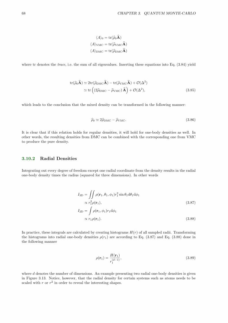
68 CHAPTER 3. QUANTUM MONTE-CARLO
〈A〉0 = tr(ρ0A)
〈A〉VMC = tr(ρVMCA)
〈A〉DMC = tr(ρDMCA)
where tr denotes the trace, i.e. the sum of all eigenvalues. Inserting these equations into Eq. (3.84) yield
tr(ρ0A) ' 2tr(ρDMCA)− tr(ρVMCA) +O(∆2)
' tr(
(2ρDMC − ρVMC) A)
+O(∆2), (3.85)
which leads to the conclusion that the mixed density can be transformed in the following manner:
ρ0 ' 2ρDMC − ρVMC. (3.86)
It is clear that if this relation holds for regular densities, it will hold for one-body densities as well. Inother words, the resulting densities from DMC can be combined with the corresponding one from VMCto produce the pure density.
3.10.2 Radial Densities
Integrating out every degree of freedom except one radial coordinate from the density results in the radialone-body density times the radius (squared for three dimensions). In other words
I3D =
∫∫ρ(r1, θ1, φ1)r2
1 sin θ1dθ1dφ1
∝ r21ρ(r1), (3.87)
I2D =
∫ρ(r1, φ1)r1dφ1
∝ r1ρ(r1). (3.88)
In practice, these integrals are calculated by creating histograms H(r) of all sampled radii. Transformingthe histograms into radial one-body densities ρ(r1) are according to Eq. (3.87) and Eq. (3.88) done inthe following manner
ρ(r1) =H(r1)
r(d−1)1
, (3.89)
where d denotes the number of dimensions. An example presenting two radial one-body densities is givenin Figure 3.13. Notice, however, that the radial density for certain systems such as atoms needs to bescaled with r or r2 in order to reveal the interesting shapes.
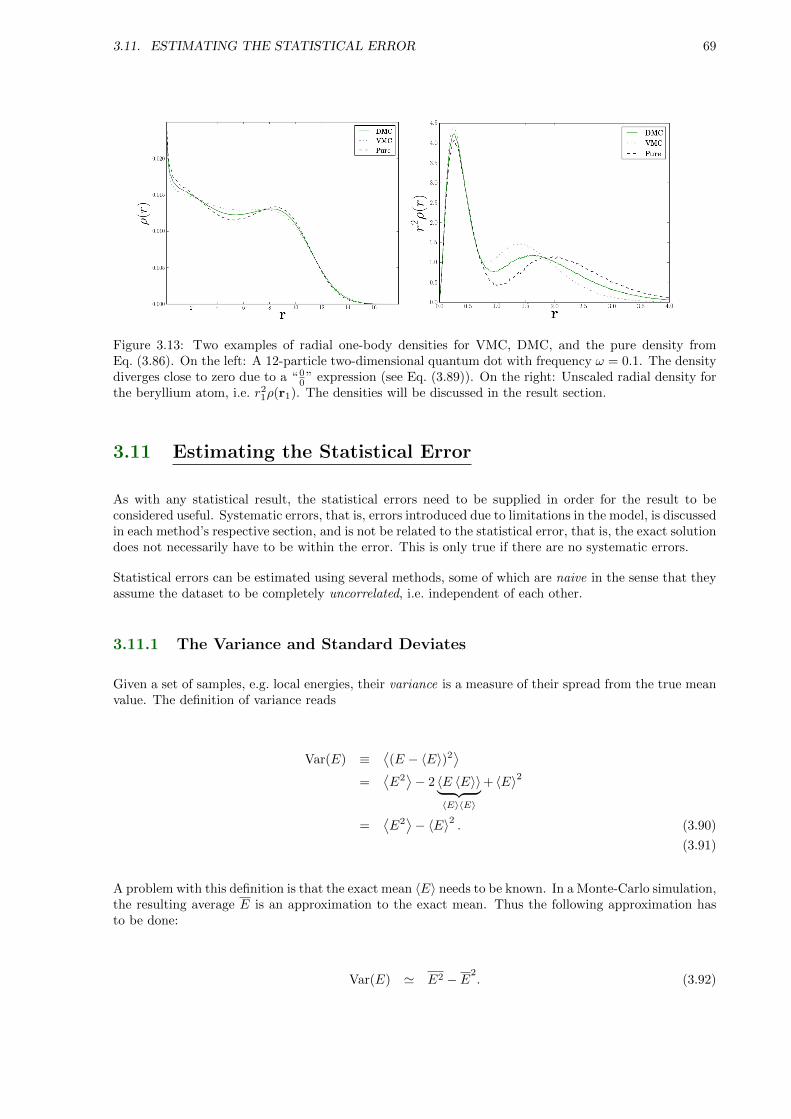
3.11. ESTIMATING THE STATISTICAL ERROR 69
Figure 3.13: Two examples of radial one-body densities for VMC, DMC, and the pure density fromEq. (3.86). On the left: A 12-particle two-dimensional quantum dot with frequency ω = 0.1. The densitydiverges close to zero due to a “ 0
0” expression (see Eq. (3.89)). On the right: Unscaled radial density forthe beryllium atom, i.e. r2
1ρ(r1). The densities will be discussed in the result section.
3.11 Estimating the Statistical Error
As with any statistical result, the statistical errors need to be supplied in order for the result to beconsidered useful. Systematic errors, that is, errors introduced due to limitations in the model, is discussedin each method’s respective section, and is not be related to the statistical error, that is, the exact solutiondoes not necessarily have to be within the error. This is only true if there are no systematic errors.
Statistical errors can be estimated using several methods, some of which are naive in the sense that theyassume the dataset to be completely uncorrelated, i.e. independent of each other.
3.11.1 The Variance and Standard Deviates
Given a set of samples, e.g. local energies, their variance is a measure of their spread from the true meanvalue. The definition of variance reads
Var(E) ≡⟨(E − 〈E〉)2
⟩=
⟨E2⟩− 2 〈E 〈E〉〉︸ ︷︷ ︸
〈E〉〈E〉
+ 〈E〉2
=⟨E2⟩− 〈E〉2 . (3.90)
(3.91)
A problem with this definition is that the exact mean 〈E〉 needs to be known. In a Monte-Carlo simulation,the resulting average E is an approximation to the exact mean. Thus the following approximation hasto be done:
Var(E) ' E2 − E2. (3.92)
70 CHAPTER 3. QUANTUM MONTE-CARLO
In the case of having the exact wave function, i.e |ΨT 〉 = |Ψ0〉, the variance becomes zero:
Var(E)Exact = 〈Ψ0| H2 |Ψ0〉 − 〈Ψ0| H |Ψ0〉2
= E20 − (E0)2
= 0
The variance is in other words an excellent measure of how close to the exact wave function the trialwave function is, hence the variance minimum is sometimes used to obtain optimal variational parametersdiscussed in Section 3.6.3.
A common misconception is that the numerical value of the variance can be used to compare propertiesof different systems. For instance, if system A has variance equal to half of system B’s, one could easilyconclude that system A has the best fitting trial wave function. However, this is not generally true. Thevariance has unit energy squared (in the case of local energies), and will thus scale with the magnitudeof the energy. One can only safely use the variance as a direct measure locally in each specific system,e.g. in simulations of the beryllium atom.
Another misconception is that the variance is a direct numerical measure of the error. This can in noway be true given that the units mismatch. The standard deviation, σ, is the square root of the variance,that is
σ2(x) = Var(x), (3.93)
and has a unit equal to that of the measured value. It is therefore related to the spread in the sampledvalue; zero deviation implies perfect samples, while increasing deviation means increasing spread andstatistical uncertainty. The standard deviation is in other words a useful quantity when it comes tocalculating the error, i.e. the expected deviation from the exact mean 〈E〉.
3.11.2 The Covariance and correlated samples
It was briefly mentioned in the introduction that certain error estimation techniques are too naive inthe sense that they do not account for samples being correlated. Two samples, x and y, are said to becorrelated if their covariance, Cov(x, y), is non-zero. The covariance is defined the following way:
Cov(x, y) ≡ 〈(x− 〈x〉)(y − 〈y〉)〉= 〈xy − x 〈y〉 − 〈x〉 y + 〈x〉 〈y〉〉= 〈xy〉 − 〈x 〈y〉〉− 〈y 〈x〉〉+ 〈〈x〉 〈y〉〉︸ ︷︷ ︸
0
= 〈xy〉 − 〈x〉 〈y〉 . (3.94)
Using this definition, whether or not the samples are correlated boils down to whether or not 〈xy〉 =〈x〉 〈y〉. Notice that the variance is the diagonal elements of the covariance matrix, i.e Cov(x, x) = Var(x).
The consequence of ignoring the correlations is an error estimate which is generally smaller than the trueerror; correlated samplings are more clustered, i.e. less spread, due to previous samples’ influence on thevalue of the current sample10. Denoting the true standard deviation as σc, the above discussion can bedistilled to
10Samples in QMC are obviously correlated due to the nature of the Langevin equation (difference equation).
3.11. ESTIMATING THE STATISTICAL ERROR 71
σc(x) ≥ σ(x), (3.95)
where σ(x) is the deviation from Eq. (3.93).
3.11.3 The Deviate from the Exact Mean
There is an important difference between the deviate from the exact mean, and the deviate of a singlesample from its combined mean. In other words:
σ(x) 6= σ(x). (3.96)
Imagine doing a number of simulations, each resulting in a unique x. The quantity of interest is notthe error of single samples, but the error in the calculated mean. Let m denote the outcome of a singleMonte-Carlo calculation. That is
m =1
n
n∑i=1
xi. (3.97)
The error in the mean is obtained by calculating the standard deviation in m. That is, calculating
σ2(m) =⟨m2⟩− 〈m〉2 . (3.98)
Combining the two above equations yield
σ2(m) =
⟨1
n2
[n∑i=1
xi
]2⟩−
⟨1
n
n∑i=1
xi
⟩2
=1
n2
⟨ n∑i=1
xi
n∑j=1
xj
⟩−
⟨n∑i=1
xi
⟩⟨n∑j=1
xj
⟩=
1
n2
n∑i,j=1
〈xixj〉 − 〈xi〉 〈xj〉
=1
n2
n∑i,j=1
Cov(xi, xj). (3.99)
This result is important; the true error is given in terms of the covariance, and is, as discussed previously,only equal to the sample variance if the samples are uncorrelated. Going back to the definition ofcovariance in Eq. (3.94), it is apparent that in order to calculate the covariance as in Eq. (3.99), the truemean 〈xi〉 needs to be known. Using m as an approximation to the exact mean yields
72 CHAPTER 3. QUANTUM MONTE-CARLO
Cov(xi, xj) = 〈(xi − 〈xi〉)(xj − 〈xj〉)〉' 〈(xi −m)(xj −m)〉
' 1
n2
n∑k,l=1
(xk −m)(xl −m) (3.100)
≡ 1
nCov(x). (3.101)
Inserting this relation into Eq. (3.99) yields
σ2(m) =1
n2
n∑i,j=1
Cov(xi, xj)
' 1
n2
n∑i,j=1
1
nCov(x)
=1
n3Cov(x)
n∑i,j=1︸︷︷︸n2
=1
nCov(x), (3.102)
which serves as an estimate of the full error including correlations.
Explicitly computing the covariance is rarely done in Monte-Carlo simulations; if the sample size is large,it is extremely expensive. A variety of alternative methods to counter the correlations are available, thesimplest of which is to define a correlation length11, τ , which defines an interval at which points from thesampling sets are used for actual averaging. In other words, only the points x0, xτ , ..., xnτ are used in thecalculation of the mean. In other words
m =1
n
n∑k=0
xk·τ . (3.103)
This implies that nτ samples are needed in order to get the same amount of samples to the average as inEq. (3.97); the effective sample size becomes neff = ntot/τ . In the cases where τ = 1, the sample set isuncorrelated. For details regarding the derivations of τ based on the covariance, see Refs. [35] and [26].
3.11.4 Blocking
Introducing correlation lengths in the system solver are not an efficient option. Neither is calculating thecovariance of billions of data points. However, the error is not a value vital to the simulation process,i.e. there is no need to know the error at any stage during the sampling. This means that the errorestimation can be done post process (given that the sample set is stored).
An efficient algorithm for calculating the error of correlated data is blocking. This method is described inhigh detail in Ref. [35], however, details aside, the idea itself is quite intuitive: Given a set of N samplesfrom a single Monte-Carlo simulation, imagine dividing the dataset into blocks of n samples, that is, into
11In literature, this parameter is often referred to as the auto-correlation time.
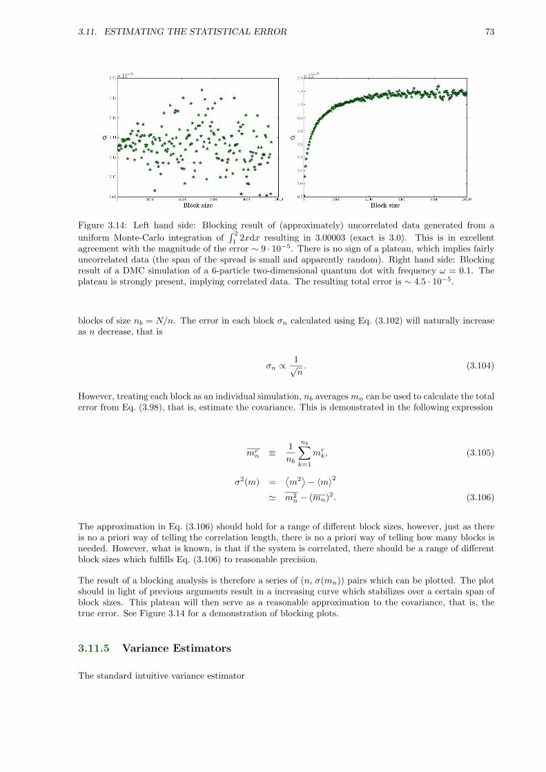
3.11. ESTIMATING THE STATISTICAL ERROR 73
Figure 3.14: Left hand side: Blocking result of (approximately) uncorrelated data generated from a
uniform Monte-Carlo integration of∫ 2
12xdx resulting in 3.00003 (exact is 3.0). This is in excellent
agreement with the magnitude of the error ∼ 9 · 10−5. There is no sign of a plateau, which implies fairlyuncorrelated data (the span of the spread is small and apparently random). Right hand side: Blockingresult of a DMC simulation of a 6-particle two-dimensional quantum dot with frequency ω = 0.1. Theplateau is strongly present, implying correlated data. The resulting total error is ∼ 4.5 · 10−5.
blocks of size nb = N/n. The error in each block σn calculated using Eq. (3.102) will naturally increaseas n decrease, that is
σn ∝1√n. (3.104)
However, treating each block as an individual simulation, nb averages mn can be used to calculate the totalerror from Eq. (3.98), that is, estimate the covariance. This is demonstrated in the following expression
mrn ≡ 1
nb
nb∑k=1
mrk, (3.105)
σ2(m) =⟨m2⟩− 〈m〉2
' m2n − (mn)2. (3.106)
The approximation in Eq. (3.106) should hold for a range of different block sizes, however, just as thereis no a priori way of telling the correlation length, there is no a priori way of telling how many blocks isneeded. However, what is known, is that if the system is correlated, there should be a range of differentblock sizes which fulfills Eq. (3.106) to reasonable precision.
The result of a blocking analysis is therefore a series of (n, σ(mn)) pairs which can be plotted. The plotshould in light of previous arguments result in a increasing curve which stabilizes over a certain span ofblock sizes. This plateau will then serve as a reasonable approximation to the covariance, that is, thetrue error. See Figure 3.14 for a demonstration of blocking plots.
3.11.5 Variance Estimators
The standard intuitive variance estimator
74 CHAPTER 3. QUANTUM MONTE-CARLO
σ2(x) ' 1
n
n∑i=1
(xi − x)2 =
(1
n
n∑i=1
x2i
)− x2, (3.107)
is just an example of a variance estimator. A more precise estimator is
σ2(x) ' 1
n− 1
n∑i=1
(xi − x)2 =
(1
n− 1
n∑i=1
x2i
)− n
n− 1x2, (3.108)
which is only noticeably different from Eq. (3.107) when the sample size gets small, as it does in blockinganalysis. It is therefore standard to use Eq. (3.108) for blocking errors.
4
Generalization and Optimization
There is a big difference in strategy between writing code for a specific problem, and creating a generalsolver. A general Quantum Monte-Carlo (QMC) solver involves several layers of complexity, such assupport for different potentials, single-particle bases, sampling models, etc., which may easily lead to acombinatorical explosion if the planning is not done right.
This chapter begins by introducing a list of underlying assumptions regarding the modelled systems.Whether or not a system can be solved is then a question of whether the listed assumptions are validfor the system or not. The next part will cover generalization, that is, the flexibility of the code and thestrategies used to obtain this flexibility. The result of a generalized code is that different systems andalgorithms can be implemented by making simple changes to the code. Finally, optimizations will becovered. Optimizations are crucial in order to maintain efficiency for a high number of particles.
4.1 Underlying Assumptions and Goals
In large computational projects it is custom to plan every single part of the program before the actualprocess of coding begins. Coding massive frameworks without planning almost exclusively result inunforeseen consequences, rendering the code difficult to expand, disorganized, and inefficient. The codeused in this thesis has been completely restructured four times. This section will cover the assumptionsregarding the modelled systems and the goals regarding generalization and optimization made in theplanning stages preliminary to the coding process.
4.1.1 Assumptions
The code structure was designed based on the following assumptions
(i) The particles of the simulated systems are either all fermions or all bosons.
(ii) The Hamiltonian is spin - and time independent.
(iii) The trial wave function of a fermionic system is a single determinant.
(iv) A bosonic system is modelled by all particles being in the same assumed single-particle groundstate.
75
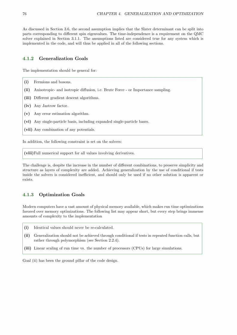
76 CHAPTER 4. GENERALIZATION AND OPTIMIZATION
As discussed in Section 3.6, the second assumption implies that the Slater determinant can be split intoparts corresponding to different spin eigenvalues. The time-independence is a requirement on the QMCsolver explained in Section 3.1.1. The assumptions listed are considered true for any system which isimplemented in the code, and will thus be applied in all of the following sections.
4.1.2 Generalization Goals
The implementation should be general for:
(i) Fermions and bosons.
(ii) Anisotropic- and isotropic diffusion, i.e. Brute Force - or Importance sampling.
(iii) Different gradient descent algorithms.
(iv) Any Jastrow factor.
(v) Any error estimation algorithm.
(vi) Any single-particle basis, including expanded single-particle bases.
(vii) Any combination of any potentials.
In addition, the following constraint is set on the solvers:
(viii)Full numerical support for all values involving derivatives.
The challenge is, despite the increase in the number of different combinations, to preserve simplicity andstructure as layers of complexity are added. Achieving generalization by the use of conditional if testsinside the solvers is considered inefficient, and should only be used if no other solution is apparent orexists.
4.1.3 Optimization Goals
Modern computers have a vast amount of physical memory available, which makes run time optimizationsfavored over memory optimizations. The following list may appear short, but every step brings immenseamounts of complexity to the implementation
(i) Identical values should never be re-calculated.
(ii) Generalization should not be achieved through conditional if tests in repeated function calls, butrather through polymorphism (see Section 2.2.4).
(iii) Linear scaling of run time vs. the number of processors (CPUs) for large simulations.
Goal (ii) has been the ground pillar of the code design.

4.2. SPECIFICS REGARDING GENERALIZATION 77
4.2 Specifics Regarding Generalization
This section will introduce how object orientation is used to achieve the goals regarding generalizationof the code. Several examples are discussed, however, for more details regarding the implementation ofmethods, see the code in Ref. [9].
4.2.1 Generalization Goals (i)-(vii)
As discussed in Section 3.6.1, the mathematical difference between fermions and bosons (of importanceto QMC) is how the many-body wave functions are constructed from the single-particle bases. In thecase of fermions, the expression is given in terms of a Slater determinant which, due to the fact that theHamiltonian is spin-independent, can be split into two parts corresponding to spin up and spin down.On the other hand, for bosons, it is simply the product of all states due to the fact that they are allassumed to occupy the same orbital. This is demonstrated in the following code example, where the wavefunctions of fermionic and bosonic systems are evaluated:
1 double Fermions :: get_spatial_wf(const Walker* walker) {
2 using namespace arma;
3
4 //Spin up times Spin down (determinants)
5 return det(walker ->phi(span(0, n2 - 1), span())) * det(walker ->phi(span(n2, n_p - 1),
span()));
6 }
7
8 double Bosons :: get_spatial_wf(const Walker* walker) {
9
10 double wf = 1;
11
12 //Using the phi matrix as a vector in the case of bosons.
13 // Assuming all particles to occupy the same single -particle state (neglecting
permutations).
14 for (int i = 0; i < n_p; i++){
15 wf *= walker ->phi(i);
16 }
17
18 return wf;
19 }
Listing 4.1: The implementation of the evaluation of fermionic and bosonic wave functions. Line 5: Thefermion class accesses the walker’s single-particle state matrix and returns the determinant of the firsthalf (spin up) times the determinant of the second half (spin down). Line 14-16: The boson class simplycalculates the product of all the single-particle states.
Overloaded pure virtual methods for fermions and bosons exist for all of the methods which involvesevaluating the many-body wave function, for example the spatial ratio and the sum of Laplacians. Whenthe QMC solver asks the System* object for a spatial ratio, depending on whether fermions or bosons areloaded run-time, the fermion or boson spatial ratio is evaluated.
It is apparent that this way of implementing the system class takes care of optimization goal (ii) in Section4.1.3 regarding no use of conditional if tests to determine the nature of the system.
A similar polymorphic splitting is introduced in the following classes:
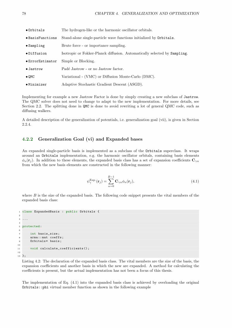
78 CHAPTER 4. GENERALIZATION AND OPTIMIZATION
• Orbitals The hydrogen-like or the harmonic oscillator orbitals.
• BasisFunctions Stand-alone single-particle wave functions initialized by Orbitals.
• Sampling Brute force - or importance sampling.
• Diffusion Isotropic or Fokker-Planck diffusion. Automatically selected by Sampling.
• ErrorEstimator Simple or Blocking.
• Jastrow Pade Jastrow - or no Jastrow factor.
• QMC Variational - (VMC) or Diffusion Monte-Carlo (DMC).
• Minimizer Adaptive Stochastic Gradient Descent (ASGD).
Implementing for example a new Jastrow Factor is done by simply creating a new subclass of Jastrow.The QMC solver does not need to change to adapt to the new implementation. For more details, seeSection 2.2. The splitting done in QMC is done to avoid rewriting a lot of general QMC code, such asdiffusing walkers.
A detailed description of the generalization of potentials, i.e. generalization goal (vii), is given in Section2.2.4.
4.2.2 Generalization Goal (vi) and Expanded bases
An expanded single-particle basis is implemented as a subclass of the Orbitals superclass. It wrapsaround an Orbitals implementation, e.g. the harmonic oscillator orbitals, containing basis elementsφα(rj). In addition to these elements, the expanded basis class has a set of expansion coefficients Cγα
from which the new basis elements are constructed in the following manner:
ψExp.γ (rj) =
B−1∑α=0
Cγαφα(rj), (4.1)
where B is the size of the expanded basis. The following code snippet presents the vital members of theexpanded basis class:
1 class ExpandedBasis : public Orbitals {
2
3 ...
4
5 protected:
6
7 int basis_size;
8 arma::mat coeffs;
9 Orbitals* basis;
10
11 void calculate_coefficients ();
12
13 };
Listing 4.2: The declaration of the expanded basis class. The vital members are the size of the basis, theexpansion coefficients and another basis in which the new are expanded. A method for calculating thecoefficients is present, but the actual implementation has not been a focus of this thesis.
The implementation of Eq. (4.1) into the expanded basis class is achieved by overloading the originalOrbitals::phi virtual member function as shown in the following example
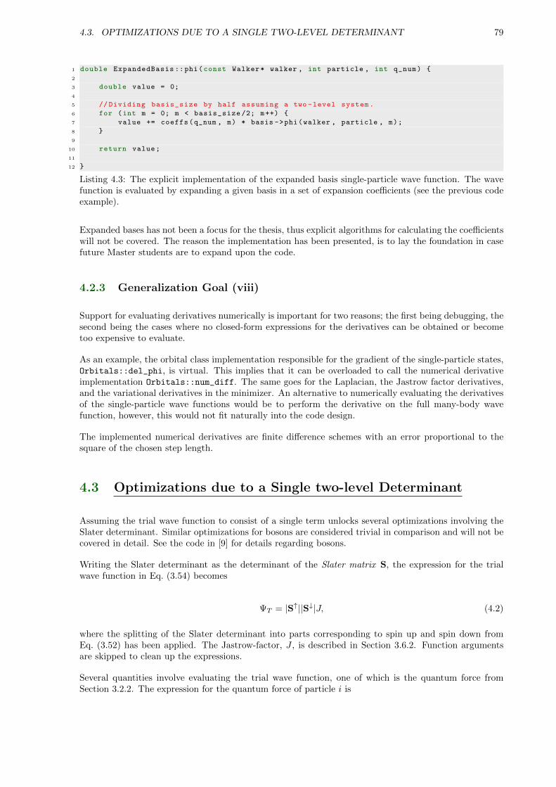
4.3. OPTIMIZATIONS DUE TO A SINGLE TWO-LEVEL DETERMINANT 79
1 double ExpandedBasis ::phi(const Walker* walker , int particle , int q_num) {
2
3 double value = 0;
4
5 // Dividing basis_size by half assuming a two -level system.
6 for (int m = 0; m < basis_size /2; m++) {
7 value += coeffs(q_num , m) * basis ->phi(walker , particle , m);
8 }
9
10 return value;
11
12 }
Listing 4.3: The explicit implementation of the expanded basis single-particle wave function. The wavefunction is evaluated by expanding a given basis in a set of expansion coefficients (see the previous codeexample).
Expanded bases has not been a focus for the thesis, thus explicit algorithms for calculating the coefficientswill not be covered. The reason the implementation has been presented, is to lay the foundation in casefuture Master students are to expand upon the code.
4.2.3 Generalization Goal (viii)
Support for evaluating derivatives numerically is important for two reasons; the first being debugging, thesecond being the cases where no closed-form expressions for the derivatives can be obtained or becometoo expensive to evaluate.
As an example, the orbital class implementation responsible for the gradient of the single-particle states,Orbitals::del_phi, is virtual. This implies that it can be overloaded to call the numerical derivativeimplementation Orbitals::num_diff. The same goes for the Laplacian, the Jastrow factor derivatives,and the variational derivatives in the minimizer. An alternative to numerically evaluating the derivativesof the single-particle wave functions would be to perform the derivative on the full many-body wavefunction, however, this would not fit naturally into the code design.
The implemented numerical derivatives are finite difference schemes with an error proportional to thesquare of the chosen step length.
4.3 Optimizations due to a Single two-level Determinant
Assuming the trial wave function to consist of a single term unlocks several optimizations involving theSlater determinant. Similar optimizations for bosons are considered trivial in comparison and will not becovered in detail. See the code in [9] for details regarding bosons.
Writing the Slater determinant as the determinant of the Slater matrix S, the expression for the trialwave function in Eq. (3.54) becomes
ΨT = |S↑||S↓|J, (4.2)
where the splitting of the Slater determinant into parts corresponding to spin up and spin down fromEq. (3.52) has been applied. The Jastrow-factor, J , is described in Section 3.6.2. Function argumentsare skipped to clean up the expressions.
Several quantities involve evaluating the trial wave function, one of which is the quantum force fromSection 3.2.2. The expression for the quantum force of particle i is
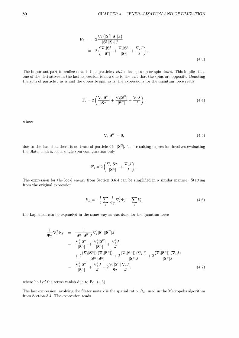
80 CHAPTER 4. GENERALIZATION AND OPTIMIZATION
Fi = 2∇i(|S↑||S↓|J
)|S↑||S↓|J
= 2
(∇i|S↑||S↑|
+∇i|S↓||S↓|
+∇iJJ
).
(4.3)
The important part to realize now, is that particle i either has spin up or spin down. This implies thatone of the derivatives in the last expression is zero due to the fact that the spins are opposite. Denotingthe spin of particle i as α and the opposite spin as α, the expressions for the quantum force reads
Fi = 2
(∇i|Sα||Sα|
+∇i|Sα||Sα|
+∇iJJ
), (4.4)
where
∇i|Sα| = 0, (4.5)
due to the fact that there is no trace of particle i in |Sα|. The resulting expression involves evaluatingthe Slater matrix for a single spin configuration only
Fi = 2
(∇i|Sα||Sα|
+∇iJJ
).
The expression for the local energy from Section 3.6.4 can be simplified in a similar manner. Startingfrom the original expression
EL = −1
2
∑i
1
ΨT∇2iΨT +
∑i
Vi, (4.6)
the Laplacian can be expanded in the same way as was done for the quantum force
1
ΨT∇2iΨT =
1
|Sα||Sα|J∇2i |Sα||Sα|J
=∇2i |Sα||Sα|
+∇2i |Sα||Sα|
+∇2iJ
J
+ 2(∇i|Sα|)
(∇i|Sα|
)|Sα||Sα|
+ 2(∇i|Sα|) (∇iJ)
|Sα|J+ 2
(∇i|Sα|
)(∇iJ)
|Sα|J
=∇2i |Sα||Sα|
+∇2iJ
J+ 2∇i|Sα||Sα|
∇iJJ
, (4.7)
where half of the terms vanish due to Eq. (4.5).
The last expression involving the Slater matrix is the spatial ratio, Rψ, used in the Metropolis algorithmfrom Section 3.4. The expression reads
4.4. OPTIMIZATIONS DUE TO SINGLE-PARTICLE MOVES 81
Rψ =ΨnewT
ΨoldT
=|S↑|new|S↓|newJnew
|S↑|old|S↓|oldJold, (4.8)
(4.9)
where the old and new superscript denotes the wave function prior to and after moving one particle,respectively. Let again i be the currently moved particle with spin α. As discussed previously, the partof the trial wave function representing the opposite spin of α, |Sα|, is independent of particle i. Thisimplies that moving particle i does not change the value of |Sα|, that is
|Sα|new = |Sα|old. (4.10)
Inserting this into Eq. (4.8) in addition to the spin parameters α and α gives
Rψ =|Sα|new
|Sα|old︸ ︷︷ ︸1
|Sα|new
|Sα|old
Jnew
Jold=|Sα|new
|Sα|old
Jnew
Jold. (4.11)
From the expressions deduced in this section it is clear that the dimensionality of the calculations is halvedby splitting the Slater determinant into two parts. Calculating the determinant of an N × N matrixcosts O(N2) floating point operations (flops), which yields a speedup of four times when estimating thedeterminants.
4.4 Optimizations due to Single-particle Moves
Moving one particle at the time implies that only a single row in the Slater determinant from Eq. (3.47)will be changed between the calculations. Changing a single row implies that many co-factors remainunchanged. Since all of the expressions deduced in the previous section contain ratios of the spatial wavefunctions, expressing these determinants in terms of their co-factors should reveal a cancellation of terms.
Expressing the cancellation mathematically presents the possibility to optimize the calculations by im-plementing only the parts which do not cancel.
In the previous section it became apparent that only the determinant whose spin level matches that ofthe moved particle needs to be calculated explicitly. In the following sections, the spin indication on theSlater matrix |Sα| will be skipped in order to clean up the equations.
4.4.1 Optimizing the Slater determinant ratio
The inverse of the Slater matrix introduced in the previous section is given in terms of its adjugate bythe following relation [36]
S−1 =1
|S|adjS.
82 CHAPTER 4. GENERALIZATION AND OPTIMIZATION
The adjugate of a matrix is the transpose of the cofactor matrix C, that is
S−1 =CT
|S|, (4.12)
S−1ij =
Cji
|S|. (4.13)
Moreover, the determinant can be expressed as a cofactor expansion around row j (Kramer’s rule) [36]
|S| =∑i
SjiCji, (4.14)
where
Sji = φi(rj). (4.15)
The spatial part of the Rψ ratio is obtained by inserting Eq. (4.14) into Eq. (4.11)
RS =
∑i S
newji Cnew
ji∑i S
oldji Cold
ji
. (4.16)
Let j represent the moved particle. The j’th column of the cofactor matrix is unchanged when the particlemoves (column j depends on every column but its own). In other words
Cnewji = Cold
ji = (Soldij )−1|Sold|, (4.17)
where the inverse relation of Eq. (4.13) has been used. Inserting this into Eq. (4.16) yields
RS =|Sold||Sold|
∑i S
newji (Sold
ij )−1∑i S
oldji (Sold
ij )−1
=
∑i S
newji (Sold
ij )−1
Ijj.
The diagonal element of the identity matrix is by definition unity. Inserting this fact combined with therelation from Eq. (4.15), an optimized expression for the ratio is obtained:
RS =∑i
φi(rnewj )(Sold
ij )−1, (4.18)
where j is the currently moved particle. The sum over i spans the Slater matrix whose spin value matchesthat of particle j, i.e either S↑ or S↓, i.e. Sα introduced in the previous section.
Similar reductions can be applied to all the Slater ratio expressions from the previous section [21,26]:
4.4. OPTIMIZATIONS DUE TO SINGLE-PARTICLE MOVES 83
∇i|S||S|
=∑k
∇iφk(rnewi )(Snew
ki )−1, (4.19)
∇2i |S||S|
=∑k
∇2iφk(rnew
i )(Snewki )−1, (4.20)
where the sum k spans the Slater matrix whose spin values match that of the moved particle.
Closed form expressions for the derivatives and Laplacians of the single-particle wave functions can beimplemented in order to avoid expensive numerical calculations. See Appendices D, E and F for atabulation of closed form expressions used in this Thesis. Appendix C presents an efficient strategy forobtaining these expressions.
4.4.2 Optimizing the inverse Slater matrix
One might question the efficiency of calculating inverse matrices compared to brute force estimationof the determinants. The efficiency of the inverse becomes apparent, as with the ratio in Eq. (4.18),by co-factor expanding the expression; an updating algorithm which dramatically decreases the cost ofcalculating the inverse of the new Slater matrix can be implemented.
Let i denote the currently moved particle. The new inverse is given in terms of the previous by thefollowing expression [21,26]
Iij =∑l
Snewil (Sold
lj )−1, (4.21)
(Snewkj )−1 = (Sold
kj )−1 − 1
RS(Soldji )−1Iij j 6= i, (4.22)
(Snewki )−1 =
1
RS(Soldki )−1 else. (4.23)
This reduces the cost of calculating the inverse by an order of magnitude down to O(N2) flops.
Further optimization can be achieved by calculating the I vector for particle i prior to performing the loopover k and j. Again, this loop should only update the inverse Slater matrix whose spin value correspondto that of the moved particle.
4.4.3 Optimizing the Pade Jastrow factor Ratio
Such as was done with the Green’s function ratio in Eq. (3.36), the ratio between two Jastrow factors arebest expressed in terms of the logarithm
logJnew
Jold=
N∑k<j=1
[akjr
newkj
1 + βrnewkj
−akjr
oldkj
1 + βroldkj
](4.24)
≡N∑
k<j=1
[gnewkj − gold
kj
]. (4.25)
84 CHAPTER 4. GENERALIZATION AND OPTIMIZATION
The relative distances rkj behave much like the cofactors in Section 4.4.1: Changing ri changes only rij ,that is
rnewkj = rold
kj k 6= i, (4.26)
which inserted into Eq. (4.25) yields
logJnew
Jold=
∑k<j 6=i
[goldkj − gold
kj
]︸ ︷︷ ︸0
+
N∑j=1
[gnewij − gold
ij
]
=
N∑j=1
aij
(rnewij
1 + βrnewij
−roldij
1 + βroldij
). (4.27)
Exponentiating both sides reveals the final optimized ratio
Jnew
Jold= exp
N∑j=1
aij
(rnewij
1 + βrnewij
−roldij
1 + βroldij
) , (4.28)
where i denotes the currently moved particle.
4.5 Optimizing the Pade Jastrow Derivative Ratios
The shape of the Pade Jastrow factor is general in the sense that it is independent of the system at hand.Calculating closed form expressions for the derivatives can then be done once and for all.
Closed form expressions are not only very efficient compared to a numerical evaluation, but also exactto machine precision. These facts render closed form expressions of high interest to any Monte-Carloimplementation.
4.5.1 The Gradient
Using the notation of Eq. (4.25), the x-component of the Pade Jastrow gradient ratio for particle i is
1
J
∂J
∂xi=
1∏k<l exp gkl
∂
∂xi
∏k<l
exp gkl. (4.29)
Using the product rule, the above product will be transformed into a sum, where only the terms whichhas k or l equal to i survive the differentiation. In addition, the terms independent of i will cancel thecorresponding terms in the denominator. Performing this calculation yields
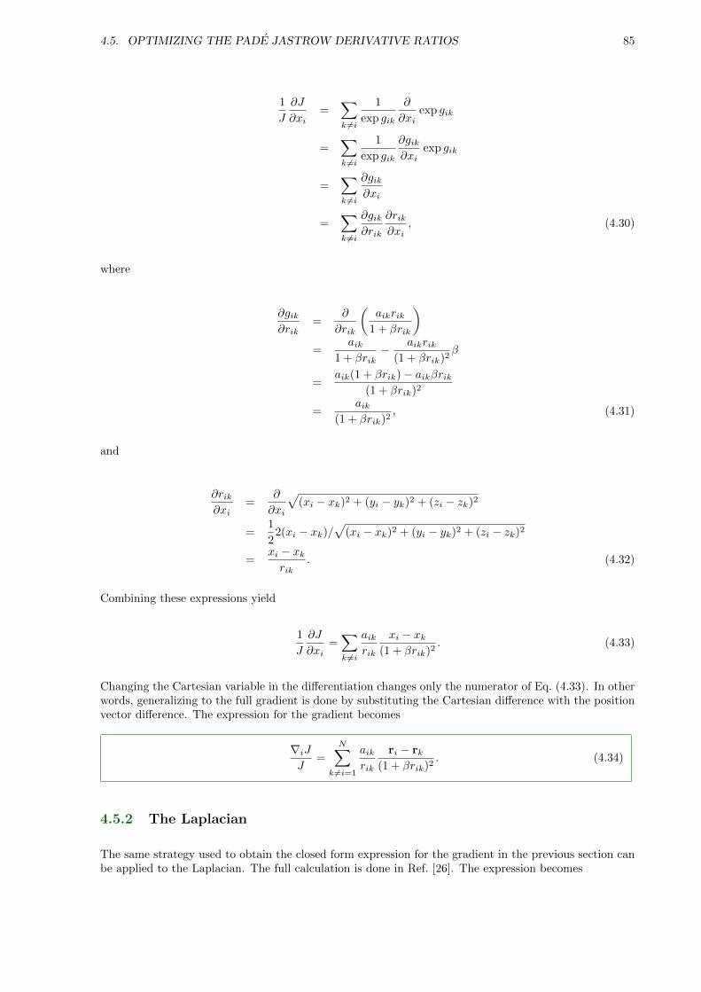
4.5. OPTIMIZING THE PADE JASTROW DERIVATIVE RATIOS 85
1
J
∂J
∂xi=
∑k 6=i
1
exp gik
∂
∂xiexp gik
=∑k 6=i
1
exp gik
∂gik∂xi
exp gik
=∑k 6=i
∂gik∂xi
=∑k 6=i
∂gik∂rik
∂rik∂xi
, (4.30)
where
∂gik∂rik
=∂
∂rik
(aikrik
1 + βrik
)=
aik1 + βrik
− aikrik(1 + βrik)2
β
=aik(1 + βrik)− aikβrik
(1 + βrik)2
=aik
(1 + βrik)2, (4.31)
and
∂rik∂xi
=∂
∂xi
√(xi − xk)2 + (yi − yk)2 + (zi − zk)2
=1
22(xi − xk)/
√(xi − xk)2 + (yi − yk)2 + (zi − zk)2
=xi − xkrik
. (4.32)
Combining these expressions yield
1
J
∂J
∂xi=∑k 6=i
aikrik
xi − xk(1 + βrik)2
. (4.33)
Changing the Cartesian variable in the differentiation changes only the numerator of Eq. (4.33). In otherwords, generalizing to the full gradient is done by substituting the Cartesian difference with the positionvector difference. The expression for the gradient becomes
∇iJJ
=
N∑k 6=i=1
aikrik
ri − rk(1 + βrik)2
. (4.34)
4.5.2 The Laplacian
The same strategy used to obtain the closed form expression for the gradient in the previous section canbe applied to the Laplacian. The full calculation is done in Ref. [26]. The expression becomes
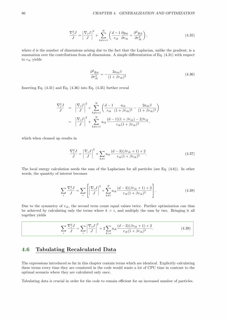
86 CHAPTER 4. GENERALIZATION AND OPTIMIZATION
∇2iJ
J=
∣∣∣∣∇iJJ∣∣∣∣2 +
N∑k 6=i=1
(d− 1
rik
∂gik∂rik
+∂2gik∂r2ik
), (4.35)
where d is the number of dimensions arising due to the fact that the Laplacian, unlike the gradient, is asummation over the contributions from all dimensions. A simple differentiation of Eq. (4.31) with respectto rik yields
∂2gik∂r2ik
= − 2aikβ
(1 + βrik)3(4.36)
Inserting Eq. (4.31) and Eq. (4.36) into Eq. (4.35) further reveal
∇2iJ
J=
∣∣∣∣∇iJJ∣∣∣∣2 +
N∑k 6=i=1
(d− 1
rik
aik(1 + βrik)2
− 2aikβ
(1 + βrik)3
)
=
∣∣∣∣∇iJJ∣∣∣∣2 +
N∑k 6=i=1
aik(d− 1)(1 + βrik)− 2βrik
rik(1 + βrik)3,
which when cleaned up results in
∇2iJ
J=
∣∣∣∣∇iJJ∣∣∣∣2 +
∑k 6=i
aik(d− 3)(βrik + 1) + 2
rik(1 + βrik)3. (4.37)
The local energy calculation needs the sum of the Laplacians for all particles (see Eq. (4.6)). In otherwords, the quantity of interest becomes
∑i
∇2iJ
J=∑i
∣∣∣∣∇iJJ∣∣∣∣2 +
N∑k 6=i
aik(d− 3)(βrik + 1) + 2
rik(1 + βrik)3
. (4.38)
Due to the symmetry of rik, the second term count equal values twice. Further optimization can thusbe achieved by calculating only the terms where k > i, and multiply the sum by two. Bringing it alltogether yields
∑i
∇2iJ
J=∑i
∣∣∣∣∇iJJ∣∣∣∣2 + 2
∑k>i
aik(d− 3)(βrik + 1) + 2
rik(1 + βrik)3. (4.39)
4.6 Tabulating Recalculated Data
The expressions introduced so far in this chapter contain terms which are identical. Explicitly calculatingthese terms every time they are countered in the code would waste a lot of CPU time in contrast to theoptimal scenario where they are calculated only once.
Tabulating data is crucial in order for the code to remain efficient for an increased number of particles.
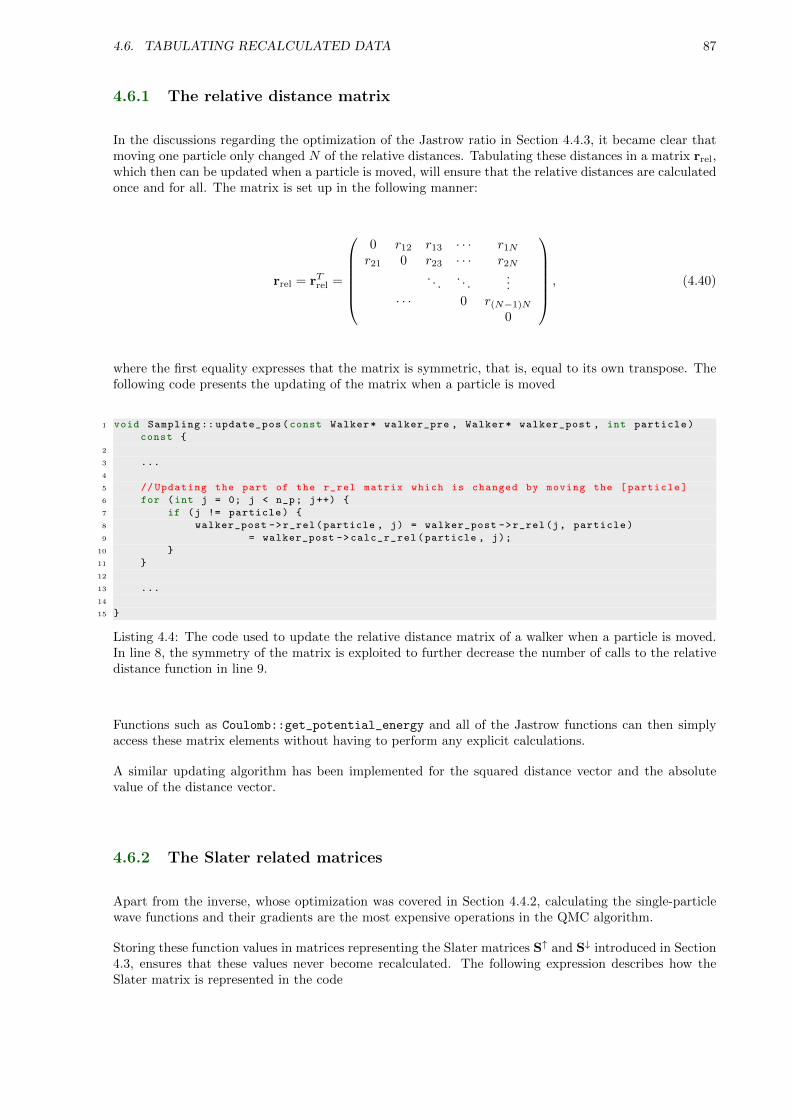
4.6. TABULATING RECALCULATED DATA 87
4.6.1 The relative distance matrix
In the discussions regarding the optimization of the Jastrow ratio in Section 4.4.3, it became clear thatmoving one particle only changed N of the relative distances. Tabulating these distances in a matrix rrel,which then can be updated when a particle is moved, will ensure that the relative distances are calculatedonce and for all. The matrix is set up in the following manner:
rrel = rTrel =
0 r12 r13 · · · r1N
r21 0 r23 · · · r2N
. . .. . .
...· · · 0 r(N−1)N
0
, (4.40)
where the first equality expresses that the matrix is symmetric, that is, equal to its own transpose. Thefollowing code presents the updating of the matrix when a particle is moved
1 void Sampling :: update_pos(const Walker* walker_pre , Walker* walker_post , int particle)
const {
2
3 ...
4
5 // Updating the part of the r_rel matrix which is changed by moving the [particle]
6 for (int j = 0; j < n_p; j++) {
7 if (j != particle) {
8 walker_post ->r_rel(particle , j) = walker_post ->r_rel(j, particle)
9 = walker_post ->calc_r_rel(particle , j);
10 }
11 }
12
13 ...
14
15 }
Listing 4.4: The code used to update the relative distance matrix of a walker when a particle is moved.In line 8, the symmetry of the matrix is exploited to further decrease the number of calls to the relativedistance function in line 9.
Functions such as Coulomb::get_potential_energy and all of the Jastrow functions can then simplyaccess these matrix elements without having to perform any explicit calculations.
A similar updating algorithm has been implemented for the squared distance vector and the absolutevalue of the distance vector.
4.6.2 The Slater related matrices
Apart from the inverse, whose optimization was covered in Section 4.4.2, calculating the single-particlewave functions and their gradients are the most expensive operations in the QMC algorithm.
Storing these function values in matrices representing the Slater matrices S↑ and S↓ introduced in Section4.3, ensures that these values never become recalculated. The following expression describes how theSlater matrix is represented in the code
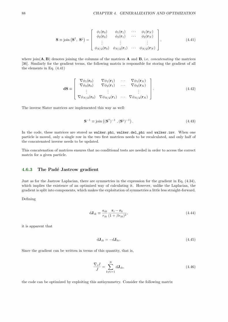
88 CHAPTER 4. GENERALIZATION AND OPTIMIZATION
S ≡ join(S↑, S↓
)=
φ1(r0) φ1(r1) · · · φ1(rN )φ2(r0) φ2(r1) · · · φ2(rN )
......
...φN/2(r0) φN/2(r1) · · · φN/2(rN )
, (4.41)
where join(A,B) denotes joining the columns of the matrices A and B, i.e. concatenating the matrices[36]. Similarly for the gradient terms, the following matrix is responsible for storing the gradient of allthe elements in Eq. (4.41)
dS ≡
∇φ1(r0) ∇φ1(r1) · · · ∇φ1(rN )∇φ2(r0) ∇φ2(r1) · · · ∇φ2(rN )
......
...∇φN/2(r0) ∇φN/2(r1) · · · ∇φN/2(rN )
. (4.42)
The inverse Slater matrices are implemented this way as well:
S−1 ≡ join((S↑)−1 , (S↓)−1
). (4.43)
In the code, these matrices are stored as walker.phi, walker.del_phi and walker.inv. When oneparticle is moved, only a single row in the two first matrices needs to be recalculated, and only half ofthe concatenated inverse needs to be updated.
This concatenation of matrices ensures that no conditional tests are needed in order to access the correctmatrix for a given particle.
4.6.3 The Pade Jastrow gradient
Just as for the Jastrow Laplacian, there are symmetries in the expression for the gradient in Eq. (4.34),which implies the existence of an optimized way of calculating it. However, unlike the Laplacian, thegradient is split into components, which makes the exploitation of symmetries a little less straight-forward.
Defining
dJik ≡aikrik
ri − rk(1 + βrik)2
, (4.44)
it is apparent that
dJik = −dJki. (4.45)
Since the gradient can be written in terms of this quantity, that is,
∇iJJ
=
N∑k 6=i=1
dJik, (4.46)
the code can be optimized by exploiting this antisymmetry. Consider the following matrix
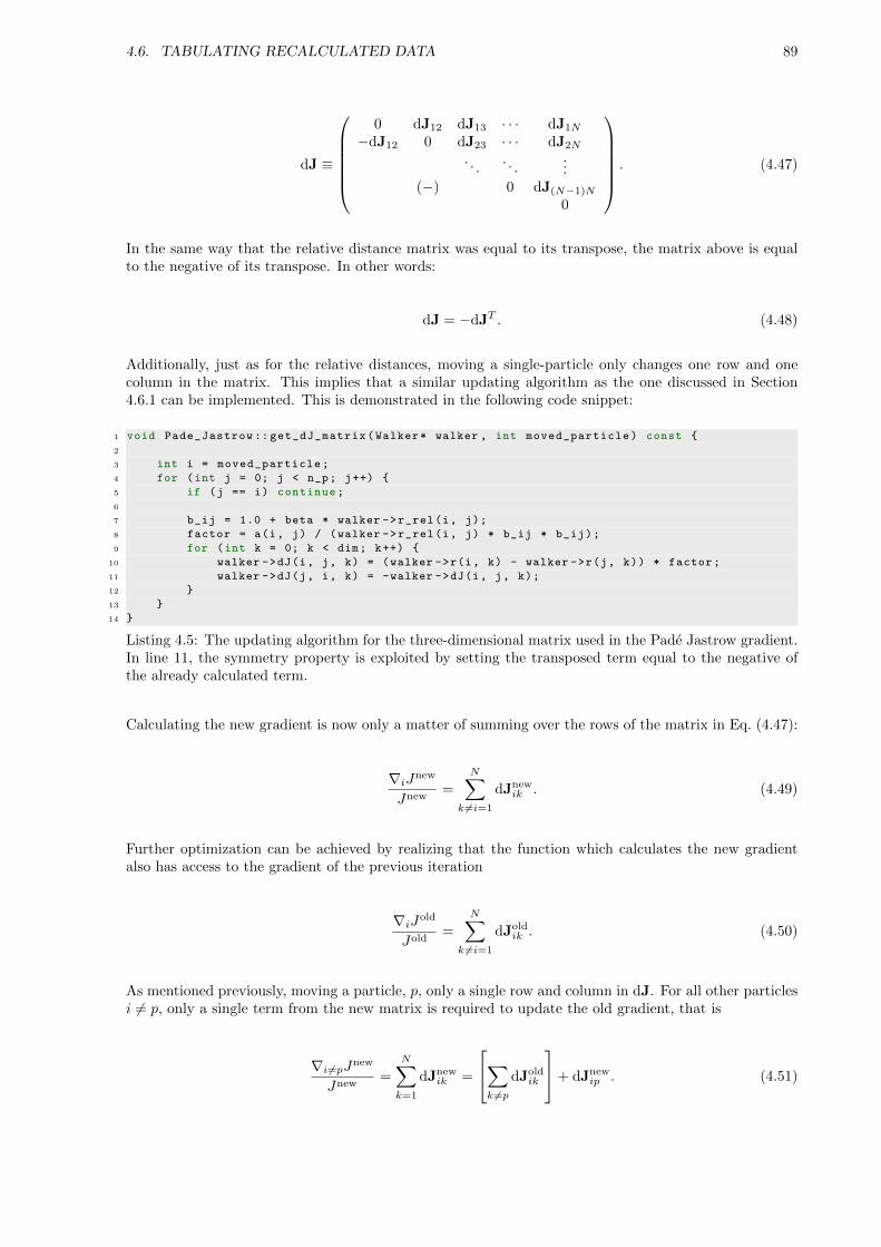
4.6. TABULATING RECALCULATED DATA 89
dJ ≡
0 dJ12 dJ13 · · · dJ1N
−dJ12 0 dJ23 · · · dJ2N
. . .. . .
...(−) 0 dJ(N−1)N
0
. (4.47)
In the same way that the relative distance matrix was equal to its transpose, the matrix above is equalto the negative of its transpose. In other words:
dJ = −dJT . (4.48)
Additionally, just as for the relative distances, moving a single-particle only changes one row and onecolumn in the matrix. This implies that a similar updating algorithm as the one discussed in Section4.6.1 can be implemented. This is demonstrated in the following code snippet:
1 void Pade_Jastrow :: get_dJ_matrix(Walker* walker , int moved_particle) const {
2
3 int i = moved_particle;
4 for (int j = 0; j < n_p; j++) {
5 if (j == i) continue;
6
7 b_ij = 1.0 + beta * walker ->r_rel(i, j);
8 factor = a(i, j) / (walker ->r_rel(i, j) * b_ij * b_ij);
9 for (int k = 0; k < dim; k++) {
10 walker ->dJ(i, j, k) = (walker ->r(i, k) - walker ->r(j, k)) * factor;
11 walker ->dJ(j, i, k) = -walker ->dJ(i, j, k);
12 }
13 }
14 }
Listing 4.5: The updating algorithm for the three-dimensional matrix used in the Pade Jastrow gradient.In line 11, the symmetry property is exploited by setting the transposed term equal to the negative ofthe already calculated term.
Calculating the new gradient is now only a matter of summing over the rows of the matrix in Eq. (4.47):
∇iJnew
Jnew=
N∑k 6=i=1
dJnewik . (4.49)
Further optimization can be achieved by realizing that the function which calculates the new gradientalso has access to the gradient of the previous iteration
∇iJold
Jold=
N∑k 6=i=1
dJoldik . (4.50)
As mentioned previously, moving a particle, p, only a single row and column in dJ. For all other particlesi 6= p, only a single term from the new matrix is required to update the old gradient, that is
∇i 6=pJnew
Jnew=
N∑k=1
dJnewik =
∑k 6=p
dJoldik
+ dJnewip . (4.51)
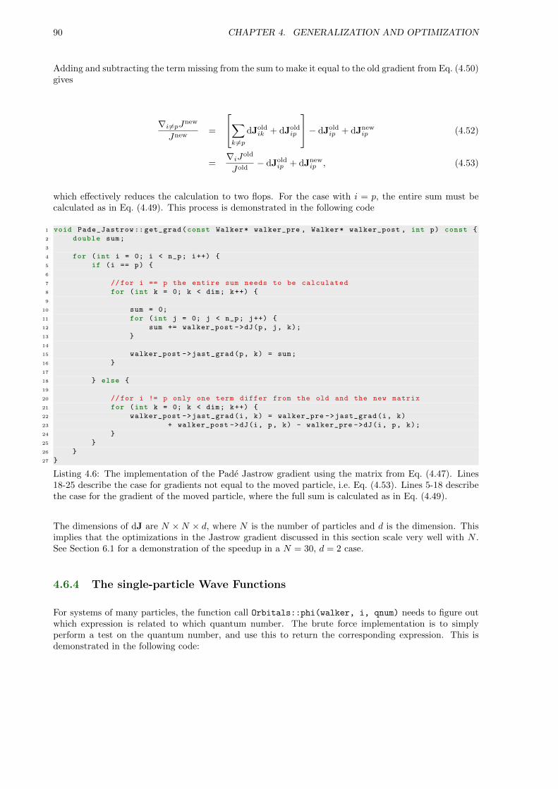
90 CHAPTER 4. GENERALIZATION AND OPTIMIZATION
Adding and subtracting the term missing from the sum to make it equal to the old gradient from Eq. (4.50)gives
∇i 6=pJnew
Jnew=
∑k 6=p
dJoldik + dJold
ip
− dJoldip + dJnew
ip (4.52)
=∇iJold
Jold− dJold
ip + dJnewip , (4.53)
which effectively reduces the calculation to two flops. For the case with i = p, the entire sum must becalculated as in Eq. (4.49). This process is demonstrated in the following code
1 void Pade_Jastrow :: get_grad(const Walker* walker_pre , Walker* walker_post , int p) const {
2 double sum;
3
4 for (int i = 0; i < n_p; i++) {
5 if (i == p) {
6
7 //for i == p the entire sum needs to be calculated
8 for (int k = 0; k < dim; k++) {
9
10 sum = 0;
11 for (int j = 0; j < n_p; j++) {
12 sum += walker_post ->dJ(p, j, k);
13 }
14
15 walker_post ->jast_grad(p, k) = sum;
16 }
17
18 } else {
19
20 //for i != p only one term differ from the old and the new matrix
21 for (int k = 0; k < dim; k++) {
22 walker_post ->jast_grad(i, k) = walker_pre ->jast_grad(i, k)
23 + walker_post ->dJ(i, p, k) - walker_pre ->dJ(i, p, k);
24 }
25 }
26 }
27 }
Listing 4.6: The implementation of the Pade Jastrow gradient using the matrix from Eq. (4.47). Lines18-25 describe the case for gradients not equal to the moved particle, i.e. Eq. (4.53). Lines 5-18 describethe case for the gradient of the moved particle, where the full sum is calculated as in Eq. (4.49).
The dimensions of dJ are N ×N × d, where N is the number of particles and d is the dimension. Thisimplies that the optimizations in the Jastrow gradient discussed in this section scale very well with N .See Section 6.1 for a demonstration of the speedup in a N = 30, d = 2 case.
4.6.4 The single-particle Wave Functions
For systems of many particles, the function call Orbitals::phi(walker, i, qnum) needs to figure outwhich expression is related to which quantum number. The brute force implementation is to simplyperform a test on the quantum number, and use this to return the corresponding expression. This isdemonstrated in the following code:
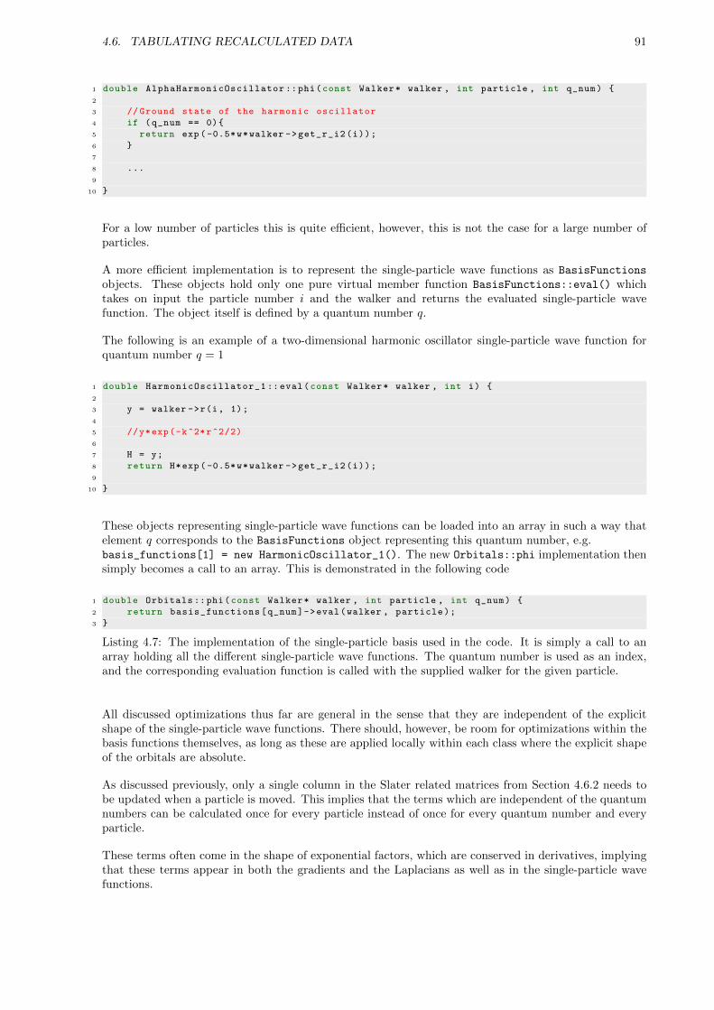
4.6. TABULATING RECALCULATED DATA 91
1 double AlphaHarmonicOscillator ::phi(const Walker* walker , int particle , int q_num) {
2
3 // Ground state of the harmonic oscillator
4 if (q_num == 0){
5 return exp(-0.5*w*walker ->get_r_i2(i));
6 }
7
8 ...
9
10 }
For a low number of particles this is quite efficient, however, this is not the case for a large number ofparticles.
A more efficient implementation is to represent the single-particle wave functions as BasisFunctions
objects. These objects hold only one pure virtual member function BasisFunctions::eval() whichtakes on input the particle number i and the walker and returns the evaluated single-particle wavefunction. The object itself is defined by a quantum number q.
The following is an example of a two-dimensional harmonic oscillator single-particle wave function forquantum number q = 1
1 double HarmonicOscillator_1 ::eval(const Walker* walker , int i) {
2
3 y = walker ->r(i, 1);
4
5 //y*exp(-k^2*r^2/2)
6
7 H = y;
8 return H*exp( -0.5*w*walker ->get_r_i2(i));
9
10 }
These objects representing single-particle wave functions can be loaded into an array in such a way thatelement q corresponds to the BasisFunctions object representing this quantum number, e.g.basis_functions[1] = new HarmonicOscillator_1(). The new Orbitals::phi implementation thensimply becomes a call to an array. This is demonstrated in the following code
1 double Orbitals ::phi(const Walker* walker , int particle , int q_num) {
2 return basis_functions[q_num]->eval(walker , particle);
3 }
Listing 4.7: The implementation of the single-particle basis used in the code. It is simply a call to anarray holding all the different single-particle wave functions. The quantum number is used as an index,and the corresponding evaluation function is called with the supplied walker for the given particle.
All discussed optimizations thus far are general in the sense that they are independent of the explicitshape of the single-particle wave functions. There should, however, be room for optimizations within thebasis functions themselves, as long as these are applied locally within each class where the explicit shapeof the orbitals are absolute.
As discussed previously, only a single column in the Slater related matrices from Section 4.6.2 needs tobe updated when a particle is moved. This implies that the terms which are independent of the quantumnumbers can be calculated once for every particle instead of once for every quantum number and everyparticle.
These terms often come in the shape of exponential factors, which are conserved in derivatives, implyingthat these terms appear in both the gradients and the Laplacians as well as in the single-particle wavefunctions.
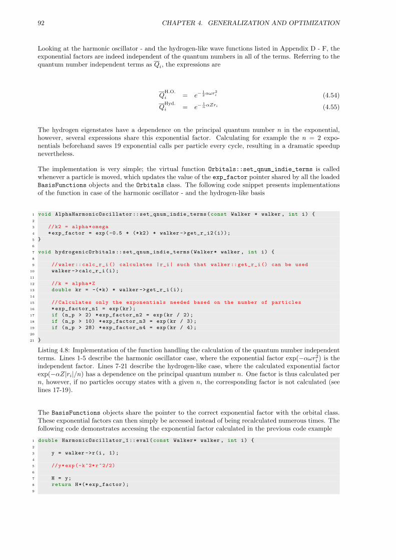
92 CHAPTER 4. GENERALIZATION AND OPTIMIZATION
Looking at the harmonic oscillator - and the hydrogen-like wave functions listed in Appendix D - F, theexponential factors are indeed independent of the quantum numbers in all of the terms. Referring to thequantum number independent terms as Qi, the expressions are
QH.O.
i = e−12αωr
2i (4.54)
QHyd.
i = e−1nαZri (4.55)
The hydrogen eigenstates have a dependence on the principal quantum number n in the exponential,however, several expressions share this exponential factor. Calculating for example the n = 2 expo-nentials beforehand saves 19 exponential calls per particle every cycle, resulting in a dramatic speedupnevertheless.
The implementation is very simple; the virtual function Orbitals::set_qnum_indie_terms is calledwhenever a particle is moved, which updates the value of the exp_factor pointer shared by all the loadedBasisFunctions objects and the Orbitals class. The following code snippet presents implementationsof the function in case of the harmonic oscillator - and the hydrogen-like basis
1 void AlphaHarmonicOscillator :: set_qnum_indie_terms(const Walker * walker , int i) {
2
3 //k2 = alpha*omega
4 *exp_factor = exp(-0.5 * (*k2) * walker ->get_r_i2(i));
5 }
6
7 void hydrogenicOrbitals :: set_qnum_indie_terms(Walker* walker , int i) {
8
9 //waler:: calc_r_i () calculates |r_i| such that walker :: get_r_i () can be used
10 walker ->calc_r_i(i);
11
12 //k = alpha*Z
13 double kr = -(*k) * walker ->get_r_i(i);
14
15 // Calculates only the exponentials needed based on the number of particles
16 *exp_factor_n1 = exp(kr);
17 if (n_p > 2) *exp_factor_n2 = exp(kr / 2);
18 if (n_p > 10) *exp_factor_n3 = exp(kr / 3);
19 if (n_p > 28) *exp_factor_n4 = exp(kr / 4);
20
21 }
Listing 4.8: Implementation of the function handling the calculation of the quantum number independentterms. Lines 1-5 describe the harmonic oscillator case, where the exponential factor exp(−αωr2
i ) is theindependent factor. Lines 7-21 describe the hydrogen-like case, where the calculated exponential factorexp(−αZ|ri|/n) has a dependence on the principal quantum number n. One factor is thus calculated pern, however, if no particles occupy states with a given n, the corresponding factor is not calculated (seelines 17-19).
The BasisFunctions objects share the pointer to the correct exponential factor with the orbital class.These exponential factors can then simply be accessed instead of being recalculated numerous times. Thefollowing code demonstrates accessing the exponential factor calculated in the previous code example
1 double HarmonicOscillator_1 ::eval(const Walker* walker , int i) {
2
3 y = walker ->r(i, 1);
4
5 //y*exp(-k^2*r^2/2)
6
7 H = y;
8 return H*(* exp_factor);
9
4.7. CPU CACHE OPTIMIZATION 93
10 }
Listing 4.9: The implementation of a single-particle wave function. The pointer to the previouslycalculated exponential factor is simply accessed in line 8.
For two-dimensional quantum dots, 112 BasisFunctions objects are needed for a 56-particle simulation.Applying the currently discussed optimization reduces the number of exponential calls needed to calculateevery wave function from 112 to 1, which for an average DMC calculation results in 6 · 1011 savedexponential calls. Generally, the number of exponential calls are reduced by a factor N
2 (N + 1), whereN is the number of particles.
4.7 CPU Cache Optimization
The CPU cache is a limited amount of memory directly connected to the CPU, designed to reduce theaverage time to access memory. Simply speaking, standard memory is slower than the CPU cache, asbits have to travel through the motherboard before it can be fed to the CPU (a so called bus).
Which values are held in the CPU cache is controlled by the compiler, however, if programmed poorly,the compiler will not be able to handle the cache storage optimally. Optimization tools such as O3 exist inorder to work around this, however, keeping the cache in mind from the beginning of the coding processmay result in a much faster code. In the case of the QMC code, the most optimal use of the cache wouldbe to have all the active walkers in the cache at all times.
The memory is sent to the cache as arrays, which means that storing walker data sequentially in memoryis the way to go in order to make take full use of the processor cache. If objects are declared as pointers,which is the case for matrices of general sizes, the memory layout is uncontrollable, that is, it is not giventhat matrices which are declared sequentially will end up sequentially in the memory. This fact rendersa QMC solver for a general number of particles hard to optimize with respect to the cache.

94
5
Modelled Systems
The systems modelled in this thesis are exclusively systems which have closed form solutions when theelectron-electron interaction is removed, i.e. in the non-interacting case. As discussed in Section 3.6,these closed form solutions are used to construct an optimal trial wave function in the form of a singleSlater determinant. Without such an optimal basis, a single Slater determinant is not sufficient inQuantum Monte-Carlo (QMC) simulations. It is therefore not random that the focus of this thesis hasbeen on various kinds of quantum dots and atomic systems, resembling the analytically solvable harmonicoscillator and the hydrogen atom, respectively.
In this chapter atomic units will be used, that is, ~ = e = me = 4πε0 = 1, where me and e0 is the electronmass and vacuum permittivity, respectively.
5.1 Atomic Systems
Atomic systems are described as a number of electrons surrounding oppositely charged nuclei. As anapproximation, the position of the nucleus is fixed. Due to the fact that the mass of the core is severalorders of magnitude larger than the mass of the electrons, this serves as a very good approximation. Inliterature this is referred to as the Born-Oppenheimer Approximation [27].
5.1.1 The Single-particle Basis
The single-particle basis used to construct the trial wave functions for atomic systems originates fromthe closed form solutions for the hydrogen atom, i.e. one electron surrounding a single nucleus.
Given a nucleus with charge Z, the external potential between the electron and the core is
vext(r) = −Zr, (5.1)
which results in the following single-particle Hamiltonian:
h0(r) = −1
2∇2 − Z
r. (5.2)
95

96 CHAPTER 5. MODELLED SYSTEMS
Figure 5.1: The one-dimensional version of the single-particle potential of hydrogen from Eq. (5.1). Thepotential is spherically symmetric for three dimensions and can be visualized by rotating the figure aroundall axes. The potential has a strong singularity at the origin, which originates from the fact that thenucleus (located at the origin) and the electrons have opposite charge, that is, they feel an attractiveforce.
The external potential is displayed in Figure 5.1. The strong singularity in the center is a result of thestrong attraction between the electron and the oppositely charged proton. The eigenfunctions of theHamiltonian are [17]
φnlm(r, θ, φ;Z) ∝ rle−Zr/n[L2l+1n−l−1
(2r
nZ
)]Y ml (θ, φ), (5.3)
where Lpq−p(x) are the associated Laguerre polynomials and Y ml (θ, φ) are the spherical harmonics. Thespherical harmonics are related to the associated Legendre functions Pml in the following manner:
Y ml (θ, φ) ∝ Pml (cos θ)eimφ, (5.4)
In the current model, the principal quantum number n together with Z control the energy level of theatom,
E(n;Z) = − Z2
2n2, (5.5)
which implies that the energy levels are degenerate for all combinations of l and m. For a given value ofn, the allowed levels of the azimuthal quantum number l and the magnetic quantum number m are
n = 1, 2, ...
l = 0, 1, ... , n− 1.
m = −l,−l + 1, ... , l − 1, l.

5.1. ATOMIC SYSTEMS 97
Different values for l and m for a given n define the shell structure of the hydrogen atom.
A problem with the single-particle basis of hydrogen is the complex terms in Eq. (5.4), i.e. the sphericalharmonics. The introduction of the solid harmonics Sml (r, θ, φ) allows for using real-valued eigenfunctionsin the QMC simulations. The solid harmonics are related to the spherical harmonics through [37]
Sml (r, θ, φ) ∝ rl[Y ml (θ, φ) + (−1)mY −ml (θ, φ)
](5.6)
∝ rlP |m|l (cos θ)
{cosmφ m ≥ 0
sin |m|φ m < 0, (5.7)
which results in the following real eigenfunctions
φnlm(r, θ, φ; k) ∝ e−kr/n[L2l+1n−l−1
(2r
nk
)]Sml (r, θ, φ) ≡ φH
nlm(r), (5.8)
where k = αZ is a scaled charge with α as a variational parameter chosen by the methods described inSection 3.6.3.
One should also keep in mind that the hydrogen-like wave functions yield only bound states. For atomswhere the least bound electrons are weakly bound, a coupling to states in the continuum may be necessary.In quantum chemistry calculations, so-called Slater orbitals are used routinely in order to account for thisdeficiency [38]. In this thesis however, the aim has been to use the given basis without tailoring it to aspecific system. This opens up the possibility to test the reliability of the basis without any fine tuning.
A set of quantum numbers nlm is mapped to a single index i. A listing of all the single-particle wavefunctions and their closed form derivatives are given in Appendix F.
5.1.2 Atoms
An atom is described as N electrons surrounding a fixed nucleus of charge Z = N . The Hamiltonianconsists of N single-particle hydrogen Hamiltonians in addition to the Coulomb interaction, which resultsin
HAtoms(r) =
N∑i=1
h0(ri) +∑i<j
1
rij(5.9)
=
N∑i=1
[−1
2∇2i −
Z
ri
]+∑i<j
1
rij, (5.10)
where rij = |ri−rj |. Excluding the Coulomb term, the Hamiltonian can be decoupled into single-particleterms with a total ground state energy
E0 = −Z2
2
N∑i=1
1
n2i
. (5.11)
The Slater determinant is set up to fill the N lowest lying states, that is, the N states with lowest nwithout breaking the Pauli principle, using the single-particle orbitals from Eq. (5.8). The degeneracy oflevel n in an atom is given by the following expression:
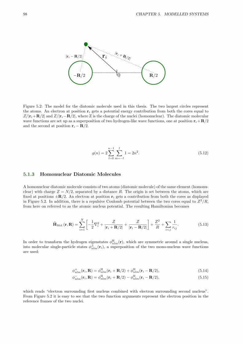
98 CHAPTER 5. MODELLED SYSTEMS
Figure 5.2: The model for the diatomic molecule used in this thesis. The two largest circles representthe atoms. An electron at position ri gets a potential energy contribution from both the cores equal toZ/|ri+R/2| and Z/|ri−R/2|, where Z is the charge of the nuclei (homonuclear). The diatomic molecularwave functions are set up as a superposition of two hydrogen-like wave functions, one at position ri+R/2and the second at position ri −R/2.
g(n) = 2
n−1∑l=0
l∑m=−l
1 = 2n2. (5.12)
5.1.3 Homonuclear Diatomic Molecules
A homonuclear diatomic molecule consists of two atoms (diatomic molecule) of the same element (homonu-clear) with charge Z = N/2, separated by a distance R. The origin is set between the atoms, which arefixed at positions ±R/2. An electron at position ri gets a contribution from both the cores as displayedin Figure 5.2. In addition, there is a repulsive Coulomb potential between the two cores equal to Z2/R,from here on referred to as the atomic nucleus potential. The resulting Hamiltonian becomes
HMol.(r,R) =
N∑i=1
[−1
2∇2i +
Z
|ri + R/2|+
Z
|ri −R/2|
]+Z2
R+∑i<j
1
rij. (5.13)
In order to transform the hydrogen eigenstates φHnlm(r), which are symmetric around a single nucleus,
into molecular single-particle states φ±nlm(ri), a superposition of the two mono-nucleus wave functionsare used:
φ+nlm(ri,R) = φH
nlm(ri + R/2) + φHnlm(ri −R/2), (5.14)
φ−nlm(ri,R) = φHnlm(ri + R/2)− φH
nlm(ri −R/2), (5.15)
which reads “electron surrounding first nucleus combined with electron surrounding second nucleus”.From Figure 5.2 it is easy to see that the two function arguments represent the electron position in thereference frames of the two nuclei.
5.2. QUANTUM DOTS 99
As seen from the equations above, there are necessarily two ways of doing this superposition: Addingand subtracting the states. It is easy to show that
⟨φ−n′l′m′ |φ+
nlm
⟩= 0, (5.16)
which implies that these states form an expanded complete set of single-particle states for the molecularsystem, resulting in a four-fold degeneracy in each set of quantum numbers nlm. It is necessary to useboth the positive and negative states in order to fit e.g. four electrons into n = 0 for the case of thelithium molecule (N = 6). Using only the positive or only the negative states would result in a singularSlater determinant.
Using R = (Rx, Ry, Rz) as the vector separating the atoms, j = (0, 1, 0) as the unit vector in the y-direction, ri = (xi, yi, zi) as the electron position, and the chain rule of derivation, the gradient in thej-direction becomes
j · ∇iφ±nlm(ri,R) =∂(yi +Ry/2)
∂yi︸ ︷︷ ︸1
∂φHnlm(ri + R/2)
∂(yi +Ry/2)
± ∂(yi −Ry/2)
∂yi︸ ︷︷ ︸1
∂φHnlm(ri −R/2)
∂(yi −Ry/2)
=∂φH
nlm(ri + R/2)
∂(yi +Ry/2)± ∂φH
nlm(ri −R/2)
∂(yi −Ry/2)
=∂φH
nlm(R+i )
∂Y +i
±∂φH
nlm(R−i )
∂Y −i, (5.17)
where R±i = ri ± R/2 = (X±i , Y±i , Z
±i ) represents the electron position in the reference frame of the
two nuclei. Equation (5.17) demonstrates that the closed form expressions used in simulations of singleatoms can be reused in the case of diatomic molecules. In other words, the functions in Appendix F cansimply be called with R±i instead of ri and then be either subtracted or added. This result holds for theLaplacian as well.
The non-interacting energy is equal to that of the regular atoms in the limit R→∞, however, now witha four-fold degeneracy and a charge equal to N/2. This four-foulding also implies that the degeneracy oflevel n becomes g(n) = 4n2.
5.2 Quantum Dots
Quantum dots are electrons confined within a potential well. This potential well can be broadened andnarrowed in such a way that the material properties of the quantum dot can be tuned to desired values.Such manufactured quantum dots have practical applications in for example solar cells [39], lasers [40],medical imaging [41], and quantum computing [42], however, the focus on quantum dots in this thesishas been purely academic.
Understanding the physics behind strongly and weakly confined electrons are of great importance whenit comes to understanding many-body theory in general. The purpose of studying quantum dots from anacademic point of view is to investigate the behavior of the system a function of the level of confinementand the number of electrons.
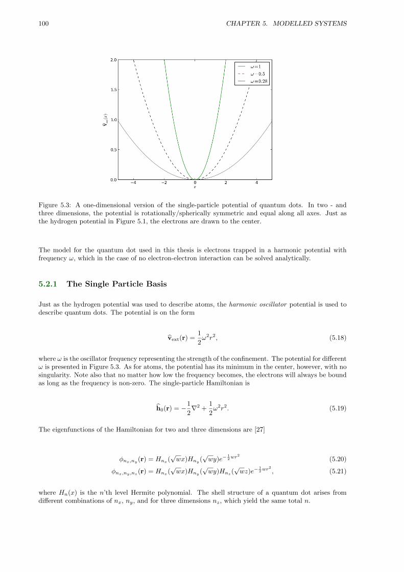
100 CHAPTER 5. MODELLED SYSTEMS
Figure 5.3: A one-dimensional version of the single-particle potential of quantum dots. In two - andthree dimensions, the potential is rotationally/spherically symmetric and equal along all axes. Just asthe hydrogen potential in Figure 5.1, the electrons are drawn to the center.
The model for the quantum dot used in this thesis is electrons trapped in a harmonic potential withfrequency ω, which in the case of no electron-electron interaction can be solved analytically.
5.2.1 The Single Particle Basis
Just as the hydrogen potential was used to describe atoms, the harmonic oscillator potential is used todescribe quantum dots. The potential is on the form
vext(r) =1
2ω2r2, (5.18)
where ω is the oscillator frequency representing the strength of the confinement. The potential for differentω is presented in Figure 5.3. As for atoms, the potential has its minimum in the center, however, with nosingularity. Note also that no matter how low the frequency becomes, the electrons will always be boundas long as the frequency is non-zero. The single-particle Hamiltonian is
h0(r) = −1
2∇2 +
1
2ω2r2. (5.19)
The eigenfunctions of the Hamiltonian for two and three dimensions are [27]
φnx,ny (r) = Hnx(√wx)Hny (
√wy)e−
12wr
2
(5.20)
φnx,ny,nz(r) = Hnx
(√wx)Hny
(√wy)Hnz
(√wz)e−
12wr
2
, (5.21)
where Hn(x) is the n’th level Hermite polynomial. The shell structure of a quantum dot arises fromdifferent combinations of nx, ny, and for three dimensions nz, which yield the same total n.
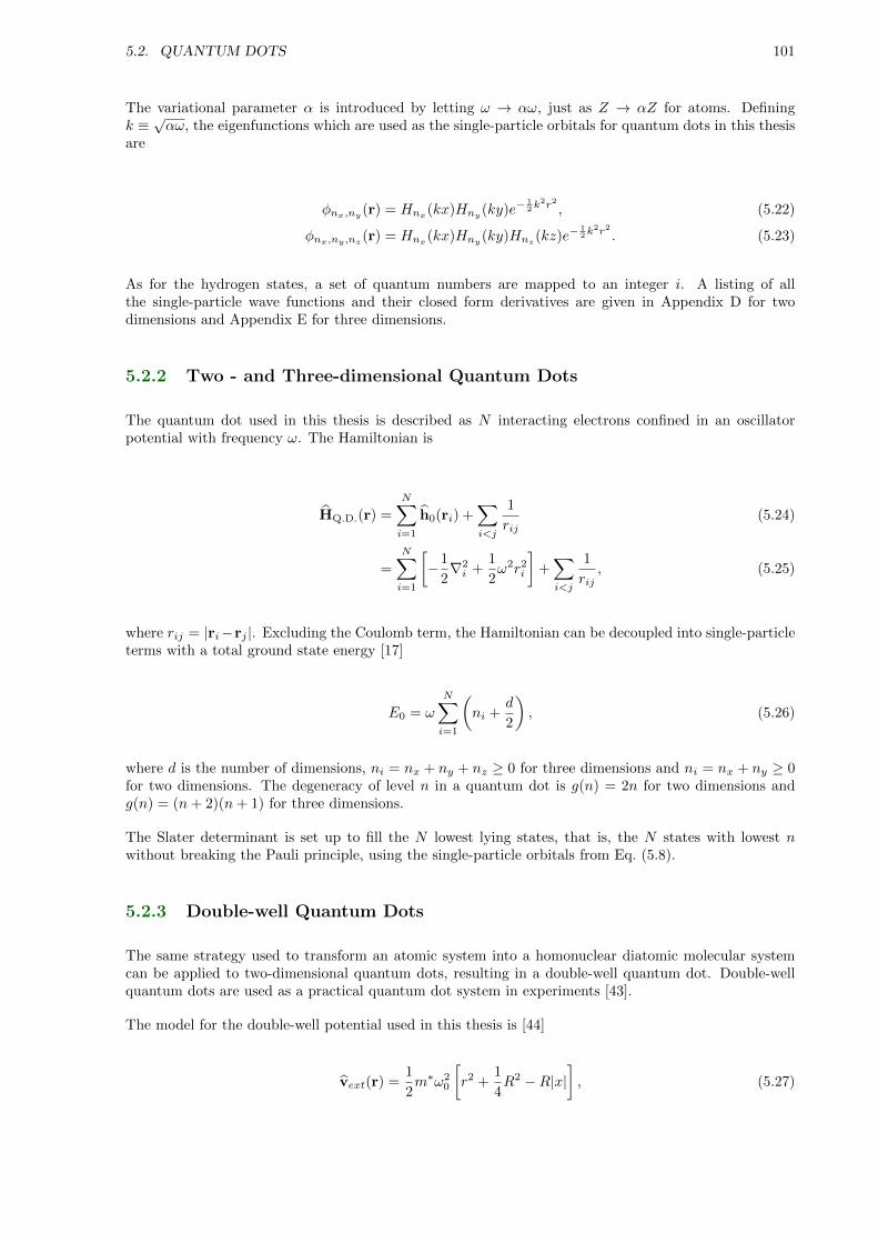
5.2. QUANTUM DOTS 101
The variational parameter α is introduced by letting ω → αω, just as Z → αZ for atoms. Definingk ≡√αω, the eigenfunctions which are used as the single-particle orbitals for quantum dots in this thesis
are
φnx,ny(r) = Hnx
(kx)Hny(ky)e−
12k
2r2 , (5.22)
φnx,ny,nz (r) = Hnx(kx)Hny (ky)Hnz (kz)e−12k
2r2 . (5.23)
As for the hydrogen states, a set of quantum numbers are mapped to an integer i. A listing of allthe single-particle wave functions and their closed form derivatives are given in Appendix D for twodimensions and Appendix E for three dimensions.
5.2.2 Two - and Three-dimensional Quantum Dots
The quantum dot used in this thesis is described as N interacting electrons confined in an oscillatorpotential with frequency ω. The Hamiltonian is
HQ.D.(r) =
N∑i=1
h0(ri) +∑i<j
1
rij(5.24)
=
N∑i=1
[−1
2∇2i +
1
2ω2r2
i
]+∑i<j
1
rij, (5.25)
where rij = |ri−rj |. Excluding the Coulomb term, the Hamiltonian can be decoupled into single-particleterms with a total ground state energy [17]
E0 = ω
N∑i=1
(ni +
d
2
), (5.26)
where d is the number of dimensions, ni = nx + ny + nz ≥ 0 for three dimensions and ni = nx + ny ≥ 0for two dimensions. The degeneracy of level n in a quantum dot is g(n) = 2n for two dimensions andg(n) = (n+ 2)(n+ 1) for three dimensions.
The Slater determinant is set up to fill the N lowest lying states, that is, the N states with lowest nwithout breaking the Pauli principle, using the single-particle orbitals from Eq. (5.8).
5.2.3 Double-well Quantum Dots
The same strategy used to transform an atomic system into a homonuclear diatomic molecular systemcan be applied to two-dimensional quantum dots, resulting in a double-well quantum dot. Double-wellquantum dots are used as a practical quantum dot system in experiments [43].
The model for the double-well potential used in this thesis is [44]
vext(r) =1
2m∗ω2
0
[r2 +
1
4R2 −R|x|
], (5.27)
102 CHAPTER 5. MODELLED SYSTEMS
Figure 5.4: The external potential for a double-well quantum dot from Eq. (5.27)with R = 2 and m∗ω2
0 = 1, where R is the distance between the well centers and m∗ and ω0 arematerial constants.
where R is the distance between the wells, m∗ is a material parameter and ω0 is the confinement strength.For simplicity, the wells are separated in the x-direction. The potential is presented in Figure 5.4.
The full Hamiltonian becomes
HQDDW(r,R) =
N∑i=1
(− 1
2m∗∇2i +
1
2m∗ω2
0
[r2 +
1
4R2 −R|xi|
])+∑i<j
1
rij, (5.28)
which can be simplified to fit the standard form of the previous Hamiltonians by letting ri →√m∗ri.
Applying this transformation of coordinates yields
HQDDW(r,R)→ HQDDW(√m∗r,
√m∗R) (5.29)
=
N∑i=1
(−1
2∇2i +
1
2ω2
0
[r2 +
1
4R2 −R|xi|
])+√m∗∑i<j
1
rij. (5.30)
The eigenstates are, as for the homonuclear diatomic molecules in Eq. (5.14) and (5.15), given as positiveand negative superpositions of the standard harmonic oscillator eigenstates. As shown for molecules inEq. (5.17), the closed form expressions for the single-well quantum dot can be reused in the case of adouble-well quantum dot.
The degeneracy of the n’th level is g(n) = 4n. The non-interacting single-particle energies are identicalto those of the single-well in the limit R→∞, that is, in the case of two decoupled potential wells.

Part II
Results
103

6
Results
The results were produced using atomic units, i.e ~ = e = me = 4πε0 = 1, where me and e0 is the electronmass and vacuum permittivity, respectively. This implies that all listed energies are given in Hartrees,i.e. scaled with ~2/mea
20, and all lengths are given in Bohr radii, i.e. scaled with a0 = 4πε0~2/mee
2.
6.1 Optimization Results
The optimization results listed in this section are estimated using a 30-particle two-dimensional quantumdot as reference system.
Profiling the code revealed that ∼ 99% of the run time was spent diffusing the particles, that is, spentin the function QMC::diffuse_walker. Variational Monte-Carlo (VMC), Diffusion Monte-Carlo (DMC),and Adaptive Stochastic Gradient Descent (ASGD) all rely heavily on the diffusion of particles, hencethe parts of the code which do not involve diffusion walkers were neglected in the optimization process;it is a waste of time to optimize something which accounts for less than one percent of the run time.
The profiling tool of choice was KCacheGrind, which is available for free at the Ubuntu Software Center.KCacheGrind lists relative time spent in functions graphically in blocks whose sizes are proportional tothe time spent inside the functions, much like standard hard drive listing software does with files and filesizes.
Optimizations discussed in Chapter 4 which are not mentioned in the following sections were consideredstandard implementations, and were thus implemented prior to the optimization process.
Storing the Slater matrix
This optimization is described in detail in Section 4.6.2. In addition to storing the Slater matrix, thecalculation of I from the inverse updating algorithm in Eq. (4.22) was taken outside of the main loops.
The percentages listed in the following table represent the ratio between the total time spent inside thegiven function and the total run time.
105

106 CHAPTER 6. RESULTS
Orbitals::phi
Relative run time used prior to optimization 80.88%Relative run time used after optimization 8.2%Relative function speedup 9.86
The speedup comes not as a result of optimizations within the function itself, but rather as a result offar less calls to the function. If I was calculated outside of the main loops in the first place, the speedupwould be far less significant.
Optimized Jastrow gradient
The optimization described in this section is discussed in detail in Section 4.6.3.
The percentages listed in the following table represent the ratio between the total time spent inside thegiven functions and the total run time.
Jastrow::get_grad & Jastrow::calc_dJ
Relative run time used prior to optimization 40%Relative run time used after optimization 5.24%Relative function speedup 7.63
Exploiting the symmetries of the Pade Jastrow gradient, in addition to calculating the new gradient basedon the old, are in other words extremely efficient. Keep in mind that these results are for a high numberof particles. For two particles, this optimization would not matter at all.
Storing the orbital derivatives
This optimization is covered in detail in Section 4.6.2. Much like for the Slater matrix, the optimizationin this case comes from the fact that the function itself is called fewer times, rather than being faster.
The percentages listed in the following table represent the ratio between the total time spent inside thegiven function and the total run time.
Orbitals.dell_phi
Relative run time used prior to optimization 56.27%Relative run time used after optimization 7.31%Relative function speedup 7.70
Storing quantum number independent terms
This optimization is covered in detail in Section 4.6.4. The result of the optimization is a reduction inthe number of exponential function calls, which means a more efficient calculation of single-paticle states,their gradients and Laplacians.
The percentages listed in the following table represent the ratio between the total time spent inside thegiven functions and the total run time.
Orbitals::phi & Orbitals::dell_phi
Relative run time used prior to optimization 5.85%Relative run time used after optimization 0.13%Relative function speedup 45
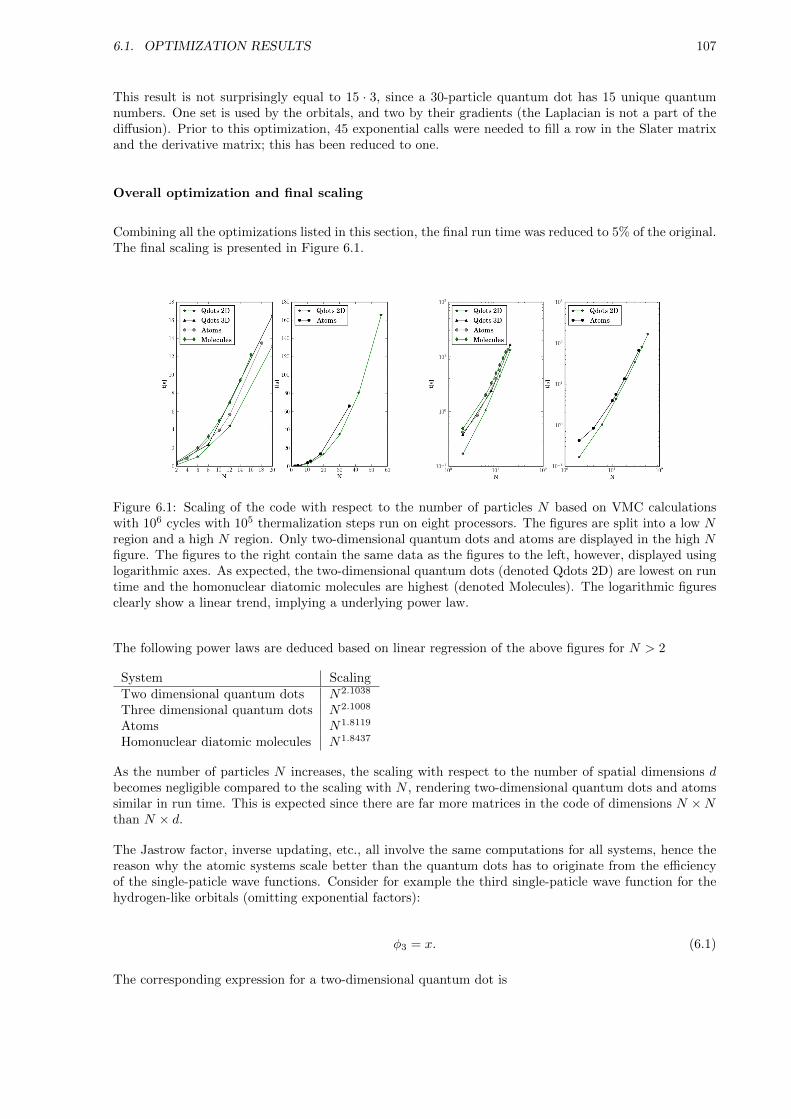
6.1. OPTIMIZATION RESULTS 107
This result is not surprisingly equal to 15 · 3, since a 30-particle quantum dot has 15 unique quantumnumbers. One set is used by the orbitals, and two by their gradients (the Laplacian is not a part of thediffusion). Prior to this optimization, 45 exponential calls were needed to fill a row in the Slater matrixand the derivative matrix; this has been reduced to one.
Overall optimization and final scaling
Combining all the optimizations listed in this section, the final run time was reduced to 5% of the original.The final scaling is presented in Figure 6.1.
Figure 6.1: Scaling of the code with respect to the number of particles N based on VMC calculationswith 106 cycles with 105 thermalization steps run on eight processors. The figures are split into a low Nregion and a high N region. Only two-dimensional quantum dots and atoms are displayed in the high Nfigure. The figures to the right contain the same data as the figures to the left, however, displayed usinglogarithmic axes. As expected, the two-dimensional quantum dots (denoted Qdots 2D) are lowest on runtime and the homonuclear diatomic molecules are highest (denoted Molecules). The logarithmic figuresclearly show a linear trend, implying a underlying power law.
The following power laws are deduced based on linear regression of the above figures for N > 2
System ScalingTwo dimensional quantum dots N2.1038
Three dimensional quantum dots N2.1008
Atoms N1.8119
Homonuclear diatomic molecules N1.8437
As the number of particles N increases, the scaling with respect to the number of spatial dimensions dbecomes negligible compared to the scaling with N , rendering two-dimensional quantum dots and atomssimilar in run time. This is expected since there are far more matrices in the code of dimensions N ×Nthan N × d.
The Jastrow factor, inverse updating, etc., all involve the same computations for all systems, hence thereason why the atomic systems scale better than the quantum dots has to originate from the efficiencyof the single-paticle wave functions. Consider for example the third single-paticle wave function for thehydrogen-like orbitals (omitting exponential factors):
φ3 = x. (6.1)
The corresponding expression for a two-dimensional quantum dot is

108 CHAPTER 6. RESULTS
φ3 = 2k2y2 − 1. (6.2)
It is obvious that the orbital for quantum dots contains a higher computational cost for the processorthan the one for atoms. Comparing the expressions listed for quantum dots in Appendix E and AppendixD with those for atoms in Appendix F, it is apparent that this trend is consistent.
The fact that the difference in the cost of the single-paticle wave functions govern the scaling demonstratesthe efficiency in the general framework. Moreover, having the molecular system scaling almost identicallyto the atomic one demonstrates the efficiency of the system’s implementation.
Both Variational Monte-Carlo and Adaptive Stochastic Gradient Descent scale linearly with the numberof processors, due to the fact that the processes do not require any communication besides adding thefinal results. Diffusion Monte-Carlo, on the other hand, is parallelized by spreading the original walkerpopulation across multiple nodes. Depending on whether some nodes have more deaths or newbornsthan others, there is a high communication cost. What is seen in practice, however, is that as long as theaverage number of walkers per node does not go below ∼ 250, the scaling is approximately linear.
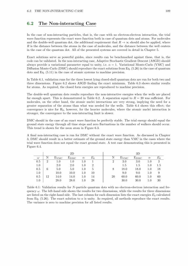
6.2. THE NON-INTERACTING CASE 109
6.2 The Non-interacting Case
In the case of non-interacting particles, that is, the case with no electron-electron interaction, the trialwave function represents the exact wave function both in case of quantum dots and atoms. For moleculesand the double-well quantum dot, the additional requirement that R→∞ should also be applied, whereR is the distance between the atoms in the case of molecules, and the distance between the well centersin the case of the quantum dot. All of the presented systems are covered in detail in Chapter 5.
Exact solutions serve as powerful guides, since results can be benchmarked against these, that is, thecode can be validated. In the non-interacting case, Adaptive Stochastic Gradient Descent (ASGD) shouldalways provide a variational parameter equal to unity, i.e. α = 1. Variational Monte-Carlo (VMC) andDiffusion Monte-Carlo (DMC) should reproduce the exact solutions from Eq. (5.26) in the case of quantumdots and Eq. (5.11) in the case of atomic systems to machine precision.
In Table 6.1, validation runs for the three lowest lying closed-shell quantum dots are run for both two andthree dimensions. Figure 6.2 shows ASGD finding the exact minimum. Table 6.3 shows similar resultsfor atoms. As required, the closed form energies are reproduced to machine precision.
The double-well quantum dots results reproduce the non-interactive energies when the wells are placedfar enough apart. This is demonstrated in Table 6.2. A separation equal to R = 20 was sufficient. Formolecules, on the other hand, the atomic nuclei interactions are very strong, implying the need for agreater separation of the atoms than what was needed for the wells. Table 6.4 shows this effect; theconvergence is nice for H2, however, for the heavier molecules, where the atomic nuclei interaction isstronger, the convergence to the non-interacting limit is slower.
DMC should in the case of an exact wave function be perfectly stable. The trial energy should equal theground state energy through all time steps and zero fluctuations in the number of walkers should occur.This trend is shown for the neon atom in Figure 6.3.
A final non-interacting case is run for DMC without the exact wave function. As discussed in Chapter3, DMC should result in a better estimate of the ground state energy than VMC in the cases where thetrial wave function does not equal the exact ground state. A test case demonstrating this is presented inFigure 6.4.
2D 3Dω N EVMC EDMC α E0 N EVMC EDMC α E0
0.5 2 1.0 1.0 1.0 1 2 3.0 3.0 1.0 31.0 2.0 2.0 1.0 2 1.5 1.5 1.0 1.50.5 6 5.0 5.0 1.0 5 8 18.0 18.0 1.0 181.0 10.0 10.0 1.0 10 9.0 9.0 1.0 90.5 12 14.0 14.0 1.0 14 20 60.0 60.0 1.0 601.0 28.0 28.0 1.0 28 30.0 30.0 1.0 30
Table 6.1: Validation results for N -particle quantum dots with no electron-electron interaction and fre-quency ω. The left-hand side shows the results for two dimensions, while the results for three dimensionsare listed on the right-hand side. The last column for each dimension lists the exact energies E0 calculatedfrom Eq. (5.26). The exact solution to α is unity. As required, all methods reproduce the exact results.The variance is zero to machine precision for all listed results.
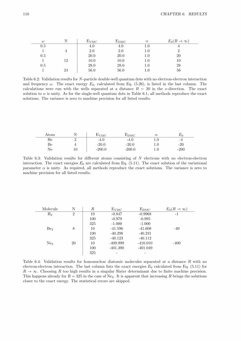
110 CHAPTER 6. RESULTS
ω N EVMC EDMC α E0(R→∞)0.5 4.0 4.0 1.0 41 4 2.0 2.0 1.0 2
0.5 20.0 20.0 1.0 201 12 10.0 10.0 1.0 10
0.5 28.0 28.0 1.0 281 24 56.0 56.0 1.0 56
Table 6.2: Validation results forN -particle double-well quantum dots with no electron-electron interactionand frequency ω. The exact energy E0, calculated from Eq. (5.26), is listed in the last column. Thecalculations were run with the wells separated at a distance R = 20 in the x-direction. The exactsolution to α is unity. As for the single-well quantum dots in Table 6.1, all methods reproduce the exactsolutions. The variance is zero to machine precision for all listed results.
Atom N EVMC EDMC α E0
He 2 -4.0 -4.0 1.0 -4Be 4 -20.0 -20.0 1.0 -20Ne 10 -200.0 -200.0 1.0 -200
Table 6.3: Validation results for different atoms consisting of N electrons with no electron-electroninteraction. The exact energies E0 are calculated from Eq. (5.11). The exact solution of the variationalparameter α is unity. As required, all methods reproduce the exact solutions. The variance is zero tomachine precision for all listed results.
Molecule N R EVMC EDMC E0(R→∞)H2 2 10 -0.847 -0.9968 -1
100 -0.979 -0.995325 -1.000 -1.000
Be2 8 10 -41.596 -41.608 -40100 -40.298 -40.231325 -40.123 -40.112
Ne2 20 10 -409.999 -410.010 -400100 -401.390 -401.049325 - -
Table 6.4: Validation results for homonuclear diatomic molecules separated at a distance R with noelectron-electron interaction. The last column lists the exact energies E0 calculated from Eq. (5.11) forR → ∞. Choosing R too high results in a singular Slater determinant due to finite machine precision.This happens already for R = 325 in the case of Ne2. It is apparent that increasing R brings the solutionscloser to the exact energy. The statistical errors are skipped.
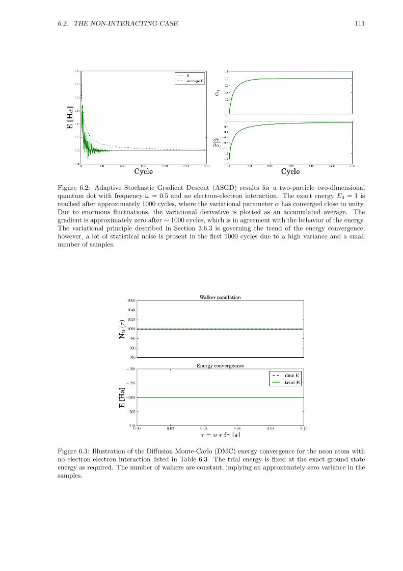
6.2. THE NON-INTERACTING CASE 111
Figure 6.2: Adaptive Stochastic Gradient Descent (ASGD) results for a two-particle two-dimensionalquantum dot with frequency ω = 0.5 and no electron-electron interaction. The exact energy E0 = 1 isreached after approximately 1000 cycles, where the variational parameter α has converged close to unity.Due to enormous fluctuations, the variational derivative is plotted as an accumulated average. Thegradient is approximately zero after ∼ 1000 cycles, which is in agreement with the behavior of the energy.The variational principle described in Section 3.6.3 is governing the trend of the energy convergence,however, a lot of statistical noise is present in the first 1000 cycles due to a high variance and a smallnumber of samples.
Figure 6.3: Illustration of the Diffusion Monte-Carlo (DMC) energy convergence for the neon atom withno electron-electron interaction listed in Table 6.3. The trial energy is fixed at the exact ground stateenergy as required. The number of walkers are constant, implying an approximately zero variance in thesamples.
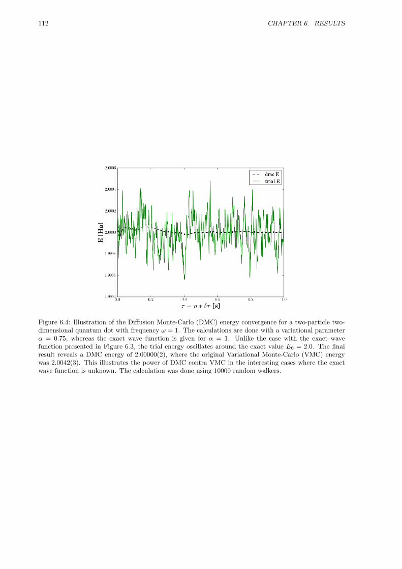
112 CHAPTER 6. RESULTS
Figure 6.4: Illustration of the Diffusion Monte-Carlo (DMC) energy convergence for a two-particle two-dimensional quantum dot with frequency ω = 1. The calculations are done with a variational parameterα = 0.75, whereas the exact wave function is given for α = 1. Unlike the case with the exact wavefunction presented in Figure 6.3, the trial energy oscillates around the exact value E0 = 2.0. The finalresult reveals a DMC energy of 2.00000(2), where the original Variational Monte-Carlo (VMC) energywas 2.0042(3). This illustrates the power of DMC contra VMC in the interesting cases where the exactwave function is unknown. The calculation was done using 10000 random walkers.
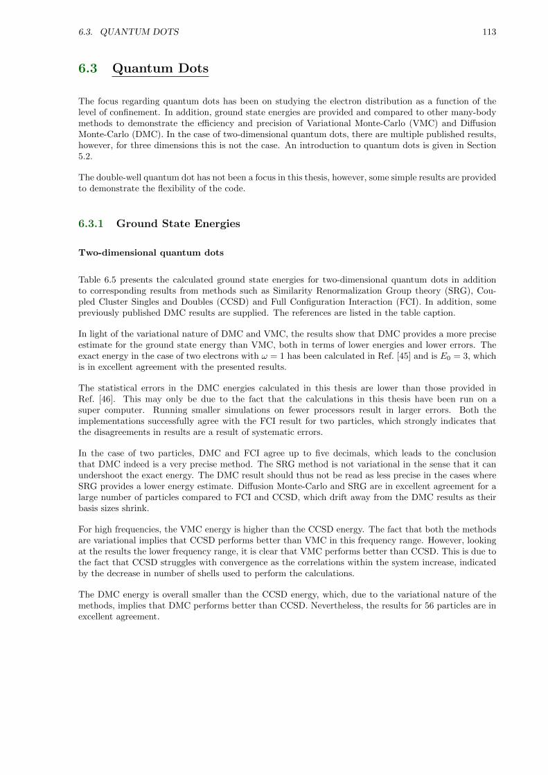
6.3. QUANTUM DOTS 113
6.3 Quantum Dots
The focus regarding quantum dots has been on studying the electron distribution as a function of thelevel of confinement. In addition, ground state energies are provided and compared to other many-bodymethods to demonstrate the efficiency and precision of Variational Monte-Carlo (VMC) and DiffusionMonte-Carlo (DMC). In the case of two-dimensional quantum dots, there are multiple published results,however, for three dimensions this is not the case. An introduction to quantum dots is given in Section5.2.
The double-well quantum dot has not been a focus in this thesis, however, some simple results are providedto demonstrate the flexibility of the code.
6.3.1 Ground State Energies
Two-dimensional quantum dots
Table 6.5 presents the calculated ground state energies for two-dimensional quantum dots in additionto corresponding results from methods such as Similarity Renormalization Group theory (SRG), Cou-pled Cluster Singles and Doubles (CCSD) and Full Configuration Interaction (FCI). In addition, somepreviously published DMC results are supplied. The references are listed in the table caption.
In light of the variational nature of DMC and VMC, the results show that DMC provides a more preciseestimate for the ground state energy than VMC, both in terms of lower energies and lower errors. Theexact energy in the case of two electrons with ω = 1 has been calculated in Ref. [45] and is E0 = 3, whichis in excellent agreement with the presented results.
The statistical errors in the DMC energies calculated in this thesis are lower than those provided inRef. [46]. This may only be due to the fact that the calculations in this thesis have been run on asuper computer. Running smaller simulations on fewer processors result in larger errors. Both theimplementations successfully agree with the FCI result for two particles, which strongly indicates thatthe disagreements in results are a result of systematic errors.
In the case of two particles, DMC and FCI agree up to five decimals, which leads to the conclusionthat DMC indeed is a very precise method. The SRG method is not variational in the sense that it canundershoot the exact energy. The DMC result should thus not be read as less precise in the cases whereSRG provides a lower energy estimate. Diffusion Monte-Carlo and SRG are in excellent agreement for alarge number of particles compared to FCI and CCSD, which drift away from the DMC results as theirbasis sizes shrink.
For high frequencies, the VMC energy is higher than the CCSD energy. The fact that both the methodsare variational implies that CCSD performs better than VMC in this frequency range. However, lookingat the results the lower frequency range, it is clear that VMC performs better than CCSD. This is due tothe fact that CCSD struggles with convergence as the correlations within the system increase, indicatedby the decrease in number of shells used to perform the calculations.
The DMC energy is overall smaller than the CCSD energy, which, due to the variational nature of themethods, implies that DMC performs better than CCSD. Nevertheless, the results for 56 particles are inexcellent agreement.
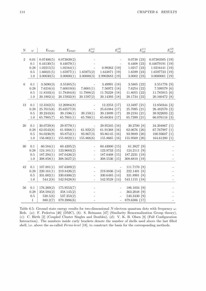
114 CHAPTER 6. RESULTS
N ω EVMC EDMC E(a)ref E
(b)ref E
(c)ref E
(d)ref
2 0.01 0.07406(5) 0.073839(2) - - 0.0738 {23} 0.07383505 {19}0.1 0.44130(5) 0.44079(1) - - 0.4408 {23} 0.44079191 {19}0.28 1.02215(5) 1.02164(1) - 0.99263 {19} 1.0217 {23} 1.0216441 {19}0.5 1.66021(5) 1.65977(1) 1.65975(2) 1.643871 {19} 1.6599 {23} 1.6597723 {19}1.0 3.00030(5) 3.00000(1) 3.00000(3) 2.9902683 {19} 3.0002 {23} 3.0000001 {19}
6 0.1 3.5690(3) 3.55385(5) - 3.49991 {18} 3.5805 {22} 3.551776 {9}0.28 7.6216(4) 7.60019(6) 7.6001(1) 7.56972 {18} 7.6254 {22} 7.599579 {6}0.5 11.8103(4) 11.78484(6) 11.7888(2) 11.76228 {18} 11.8055 {22} 11.785915 {6}1.0 20.1902(4) 20.15932(8) 20.1597(2) 20.14393 {18} 20.1734 {22} 20.160472 {8}
12 0.1 12.3162(5) 12.26984(8) - 12.2253 {17} 12.3497 {21} 12.850344 {3}0.28 25.7015(6) 25.63577(9) - 25.61084 {17} 25.7095 {21} 26.482570 {2}0.5 39.2343(6) 39.1596(1) 39.159(1) 39.13899 {17} 39.2194 {21} 39.922693 {2}1.0 65.7905(7) 65.7001(1) 65.700(1) 65.68304 {17} 65.7399 {21} 66.076116 {3}
20 0.1 30.0729(8) 29.9779(1) - 29.95345 {16} 30.2700 {8} 34.204867 {1}0.28 62.0543(8) 61.9268(1) 61.922(2) 61.91368 {16} 62.0676 {20} 67.767987 {1}0.5 94.0236(9) 93.8752(1) 93.867(3) 93.86145 {16} 93.9889 {20} 100.93607 {1}1.0 156.062(1) 155.8822(1) 155.868(6) 155.8665 {16} 155.9569 {20} 164.61280 {1}
30 0.1 60.584(1) 60.4205(2) - 60.43000 {15} 61.3827 {9} -0.28 124.181(1) 123.9683(2) - 123.9733 {15} 124.2111 {9} -0.5 187.294(1) 187.0426(2) - 187.0408 {15} 187.2231 {19} -1.0 308.858(1) 308.5627(2) - 308.5536 {15} 308.6810 {19} -
42 0.1 107.881(1) 107.6389(2) - - 111.7170 {8} -0.28 220.161(1) 219.8426(2) - 219.8836 {14} 222.1401 {8} -0.5 331.002(1) 330.6306(2) - 330.6485 {14} 331.8901 {8} -1.0 544.2(8) 542.9428(8) - 542.9528 {14} 543.1155 {18} -
56 0.1 176.269(2) 175.9553(7) - - 186.1034 {9} -0.28 358.594(2) 358.145(2) - - 363.2048 {9} -0.5 538.5(6) 537.353(2) - - 540.3430 {9} -1 880.2(7) 879.3986(6) - - 879.6386 {17} -
Table 6.5: Ground state energy results for two-dimensional N -electron quantum dots with frequency ω.Refs. (a): F. Pederiva [46] (DMC), (b): S. Reimann [47] (Similarity Renormalization Group theory),(c): C. Hirth [2] (Coupled Cluster Singles and Doubles), (d): V. K. B. Olsen [8] (Full ConfigurationInteraction). The numbers inside curly brackets denote the number of shells used above the last filledshell, i.e. above the so-called Fermi-level [18], to construct the basis for the corresponding methods.
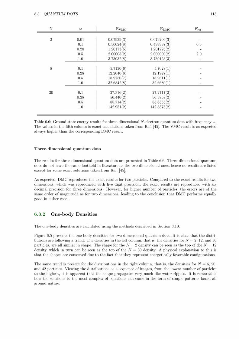
6.3. QUANTUM DOTS 115
N ω EVMC EDMC Eref
2 0.01 0.07939(3) 0.079206(3) -0.1 0.50024(8) 0.499997(3) 0.50.28 1.20173(5) 1.201725(2) -0.5 2.00005(2) 2.000000(2) 2.01.0 3.73032(8) 3.730123(3) -
8 0.1 5.7130(6) 5.7028(1) -0.28 12.2040(8) 12.1927(1) -0.5 18.9750(7) 18.9611(1) -1.0 32.6842(8) 32.6680(1) -
20 0.1 27.316(2) 27.2717(2) -0.28 56.440(2) 56.3868(2) -0.5 85.714(2) 85.6555(2) -1.0 142.951(2) 142.8875(2) -
Table 6.6: Ground state energy results for three-dimensional N -electron quantum dots with frequency ω.The values in the fifth column is exact calculations taken from Ref. [45]. The VMC result is as expectedalways higher than the corresponding DMC result.
Three-dimensional quantum dots
The results for three-dimensional quantum dots are presented in Table 6.6. Three-dimensional quantumdots do not have the same foothold in literature as the two-dimensional ones, hence no results are listedexcept for some exact solutions taken from Ref. [45].
As expected, DMC reproduces the exact results for two particles. Compared to the exact results for twodimensions, which was reproduced with five digit precision, the exact results are reproduced with sixdecimal precision for three dimensions. However, for higher number of particles, the errors are of thesame order of magnitude as for two dimensions, leading to the conclusion that DMC performs equallygood in either case.
6.3.2 One-body Densities
The one-body densities are calculated using the methods described in Section 3.10.
Figure 6.5 presents the one-body densities for two-dimensional quantum dots. It is clear that the distri-butions are following a trend: The densities in the left column, that is, the densities for N = 2, 12, and 30particles, are all similar in shape. The shape for the N = 2 density can be seen as the top of the N = 12density, which in turn can be seen as the top of the N = 30 density. A physical explanation to this isthat the shapes are conserved due to the fact that they represent energetically favorable configurations.
The same trend is present for the distributions in the right column, that is, the densities for N = 6, 20,and 42 particles. Viewing the distributions as a sequence of images, from the lowest number of particlesto the highest, it is apparent that the shape propagates very much like water ripples. It is remarkablehow the solutions to the most complex of equations can come in the form of simple patterns found allaround nature.
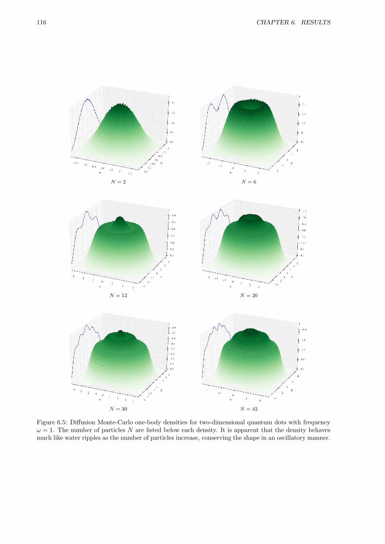
116 CHAPTER 6. RESULTS
N = 2 N = 6
N = 12 N = 20
N = 30 N = 42
Figure 6.5: Diffusion Monte-Carlo one-body densities for two-dimensional quantum dots with frequencyω = 1. The number of particles N are listed below each density. It is apparent that the density behavesmuch like water ripples as the number of particles increase, conserving the shape in an oscillatory manner.
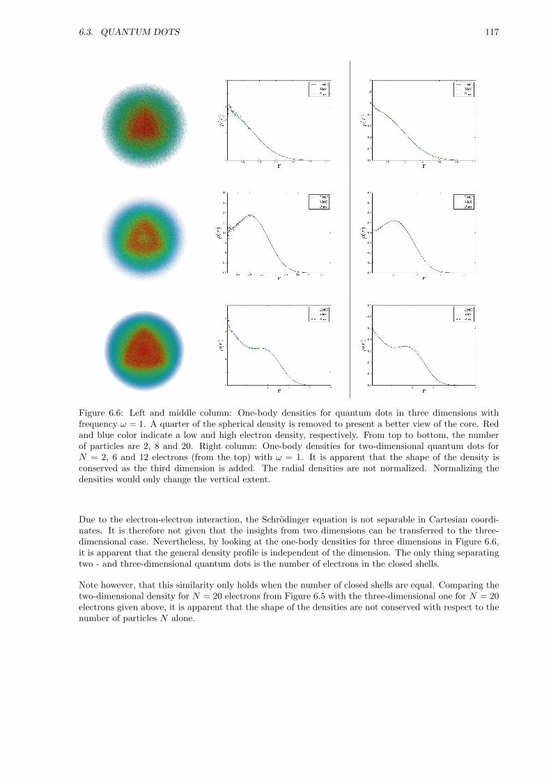
6.3. QUANTUM DOTS 117
Figure 6.6: Left and middle column: One-body densities for quantum dots in three dimensions withfrequency ω = 1. A quarter of the spherical density is removed to present a better view of the core. Redand blue color indicate a low and high electron density, respectively. From top to bottom, the numberof particles are 2, 8 and 20. Right column: One-body densities for two-dimensional quantum dots forN = 2, 6 and 12 electrons (from the top) with ω = 1. It is apparent that the shape of the density isconserved as the third dimension is added. The radial densities are not normalized. Normalizing thedensities would only change the vertical extent.
Due to the electron-electron interaction, the Schrodinger equation is not separable in Cartesian coordi-nates. It is therefore not given that the insights from two dimensions can be transferred to the three-dimensional case. Nevertheless, by looking at the one-body densities for three dimensions in Figure 6.6,it is apparent that the general density profile is independent of the dimension. The only thing separatingtwo - and three-dimensional quantum dots is the number of electrons in the closed shells.
Note however, that this similarity only holds when the number of closed shells are equal. Comparing thetwo-dimensional density for N = 20 electrons from Figure 6.5 with the three-dimensional one for N = 20electrons given above, it is apparent that the shape of the densities are not conserved with respect to thenumber of particles N alone.
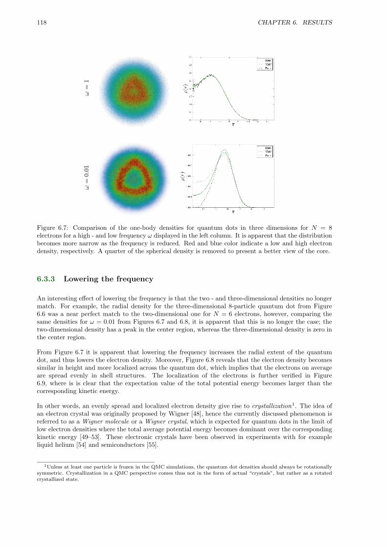
118 CHAPTER 6. RESULTS
ω=
1ω
=0.
01
Figure 6.7: Comparison of the one-body densities for quantum dots in three dimensions for N = 8electrons for a high - and low frequency ω displayed in the left column. It is apparent that the distributionbecomes more narrow as the frequency is reduced. Red and blue color indicate a low and high electrondensity, respectively. A quarter of the spherical density is removed to present a better view of the core.
6.3.3 Lowering the frequency
An interesting effect of lowering the frequency is that the two - and three-dimensional densities no longermatch. For example, the radial density for the three-dimensional 8-particle quantum dot from Figure6.6 was a near perfect match to the two-dimensional one for N = 6 electrons, however, comparing thesame densities for ω = 0.01 from Figures 6.7 and 6.8, it is apparent that this is no longer the case; thetwo-dimensional density has a peak in the center region, whereas the three-dimensional density is zero inthe center region.
From Figure 6.7 it is apparent that lowering the frequency increases the radial extent of the quantumdot, and thus lowers the electron density. Moreover, Figure 6.8 reveals that the electron density becomessimilar in height and more localized across the quantum dot, which implies that the electrons on averageare spread evenly in shell structures. The localization of the electrons is further verified in Figure6.9, where is is clear that the expectation value of the total potential energy becomes larger than thecorresponding kinetic energy.
In other words, an evenly spread and localized electron density give rise to crystallization1. The idea ofan electron crystal was originally proposed by Wigner [48], hence the currently discussed phenomenon isreferred to as a Wigner molecule or a Wigner crystal, which is expected for quantum dots in the limit oflow electron densities where the total average potential energy becomes dominant over the correspondingkinetic energy [49–53]. These electronic crystals have been observed in experiments with for exampleliquid helium [54] and semiconductors [55].
1Unless at least one particle is frozen in the QMC simulations, the quantum dot densities should always be rotationallysymmetric. Crystallization in a QMC perspective comes thus not in the form of actual “crystals”, but rather as a rotatedcrystallized state.
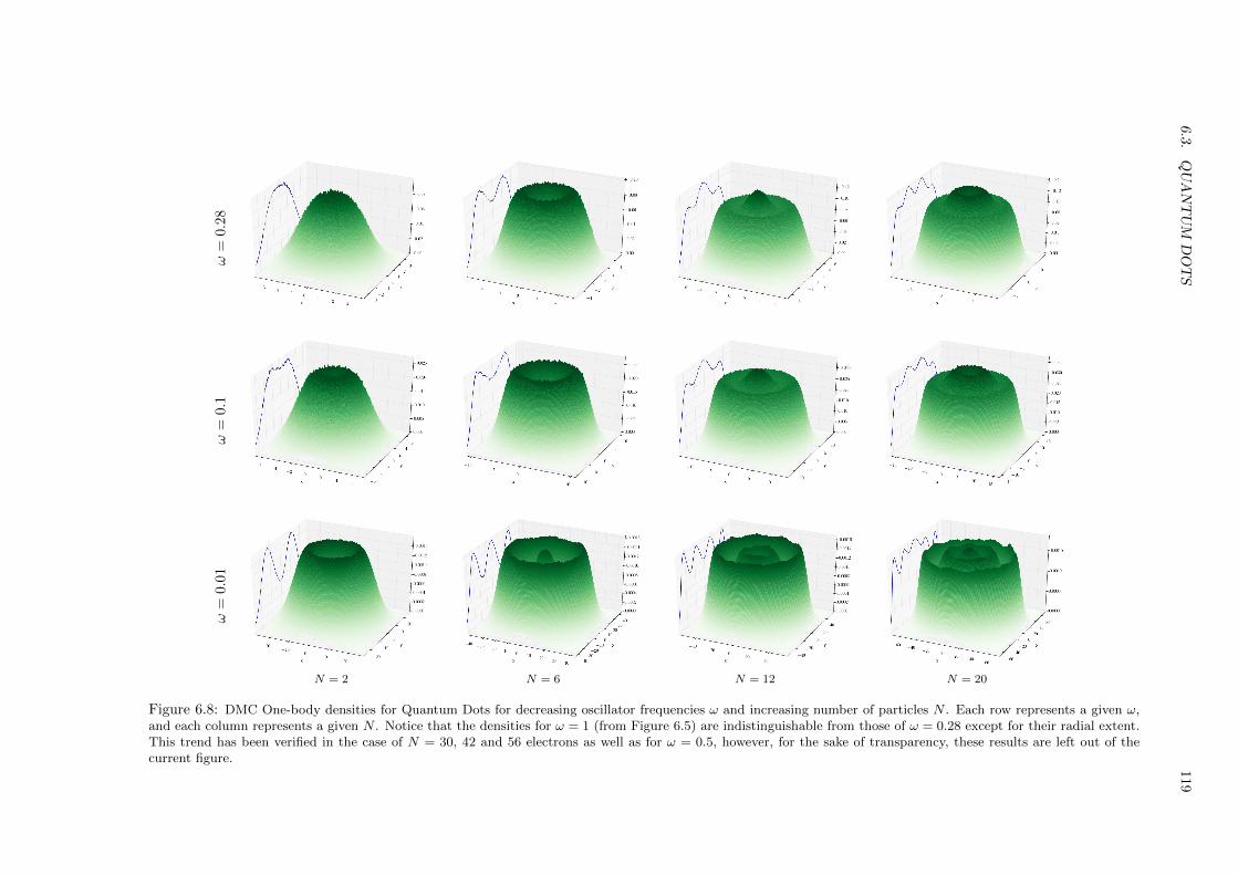
6.3.
QU
AN
TU
MD
OT
S119
ω=
0.28
ω=
0.1
ω=
0.01
N = 2 N = 6 N = 12 N = 20
Figure 6.8: DMC One-body densities for Quantum Dots for decreasing oscillator frequencies ω and increasing number of particles N . Each row represents a given ω,and each column represents a given N . Notice that the densities for ω = 1 (from Figure 6.5) are indistinguishable from those of ω = 0.28 except for their radial extent.This trend has been verified in the case of N = 30, 42 and 56 electrons as well as for ω = 0.5, however, for the sake of transparency, these results are left out of thecurrent figure.
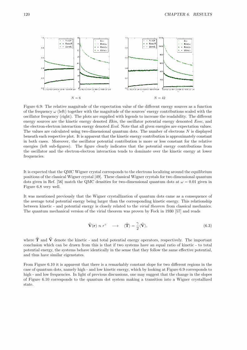
120 CHAPTER 6. RESULTS
N = 6 N = 42
Figure 6.9: The relative magnitude of the expectation value of the different energy sources as a functionof the frequency ω (left) together with the magnitude of the sources’ energy contributions scaled with theoscillator frequency (right). The plots are supplied with legends to increase the readability. The differentenergy sources are the kinetic energy denoted Ekin, the oscillator potential energy denonted Eosc, andthe electron-electron interaction energy denoted Ecol. Note that all given energies are expectation values.The values are calculated using two-dimensional quantum dots. The number of electrons N is displayedbeneath each respective plot. It is apparent that the kinetic energy contribution is approximately constantin both cases. Moreover, the oscillator potential contribution is more or less constant for the relativeenergies (left sub-figures). The figure clearly indicates that the potential energy contributions fromthe oscillator and the electron-electron interaction tends to dominate over the kinetic energy at lowerfrequencies.
It is expected that the QMC Wigner crystal corresponds to the electrons localizing around the equilibriumpositions of the classical Wigner crystal [49]. These classical Wigner crystals for two dimensional quantumdots given in Ref. [56] match the QMC densities for two-dimensional quantum dots at ω = 0.01 given inFigure 6.8 very well.
It was mentioned previously that the Wigner crystallization of quantum dots came as a consequence ofthe average total potential energy being larger than the corresponding kinetic energy. This relationshipbetween kinetic - and potential energy is closely related to the virial theorem from classical mechanics.The quantum mechanical version of the virial theorem was proven by Fock in 1930 [57] and reads
V(r) ∝ rγ −→ 〈T〉 =γ
2〈V〉, (6.3)
where T and V denote the kinetic - and total potential energy operators, respectively. The importantconclusion which can be drawn from this is that if two systems have an equal ratio of kinetic - to totalpotential energy, the systems behave identically in the sense that they follow the same effective potential,and thus have similar eigenstates.
From Figure 6.10 it is apparent that there is a remarkably constant slope for two different regions in thecase of quantum dots, namely high - and low kinetic energy, which by looking at Figure 6.9 corresponds tohigh - and low frequencies. In light of previous discussions, one may suggest that the change in the slopesof Figure 6.10 corresponds to the quantum dot system making a transition into a Wigner crystallizedstate.
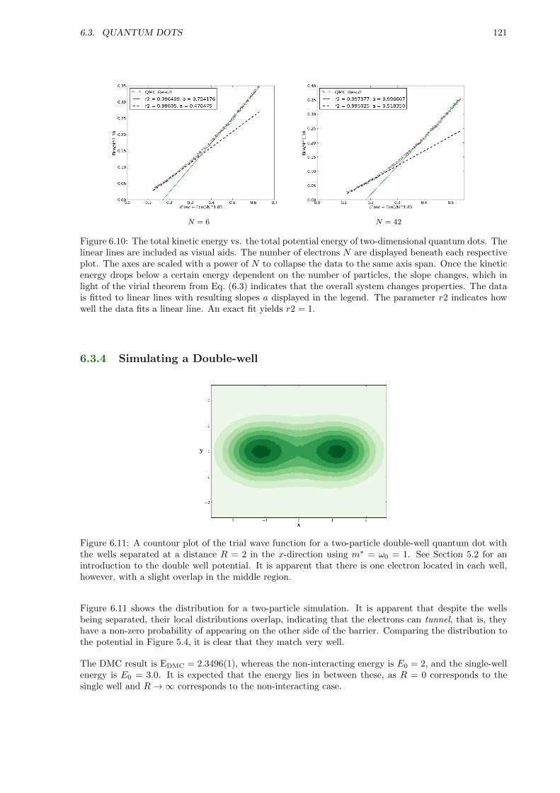
6.3. QUANTUM DOTS 121
N = 6 N = 42
Figure 6.10: The total kinetic energy vs. the total potential energy of two-dimensional quantum dots. Thelinear lines are included as visual aids. The number of electrons N are displayed beneath each respectiveplot. The axes are scaled with a power of N to collapse the data to the same axis span. Once the kineticenergy drops below a certain energy dependent on the number of particles, the slope changes, which inlight of the virial theorem from Eq. (6.3) indicates that the overall system changes properties. The datais fitted to linear lines with resulting slopes a displayed in the legend. The parameter r2 indicates howwell the data fits a linear line. An exact fit yields r2 = 1.
6.3.4 Simulating a Double-well
Figure 6.11: A countour plot of the trial wave function for a two-particle double-well quantum dot withthe wells separated at a distance R = 2 in the x-direction using m∗ = ω0 = 1. See Section 5.2 for anintroduction to the double well potential. It is apparent that there is one electron located in each well,however, with a slight overlap in the middle region.
Figure 6.11 shows the distribution for a two-particle simulation. It is apparent that despite the wellsbeing separated, their local distributions overlap, indicating that the electrons can tunnel, that is, theyhave a non-zero probability of appearing on the other side of the barrier. Comparing the distribution tothe potential in Figure 5.4, it is clear that they match very well.
The DMC result is EDMC = 2.3496(1), whereas the non-interacting energy is E0 = 2, and the single-wellenergy is E0 = 3.0. It is expected that the energy lies in between these, as R = 0 corresponds to thesingle well and R→∞ corresponds to the non-interacting case.
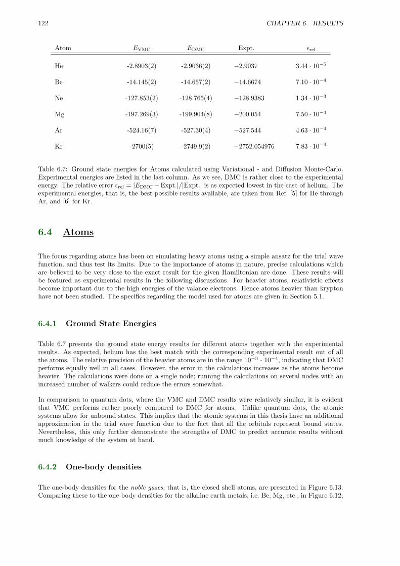
122 CHAPTER 6. RESULTS
Atom EVMC EDMC Expt. εrel
He -2.8903(2) -2.9036(2) −2.9037 3.44 · 10−5
Be -14.145(2) -14.657(2) −14.6674 7.10 · 10−4
Ne -127.853(2) -128.765(4) −128.9383 1.34 · 10−3
Mg -197.269(3) -199.904(8) −200.054 7.50 · 10−4
Ar -524.16(7) -527.30(4) −527.544 4.63 · 10−4
Kr -2700(5) -2749.9(2) −2752.054976 7.83 · 10−4
Table 6.7: Ground state energies for Atoms calculated using Variational - and Diffusion Monte-Carlo.Experimental energies are listed in the last column. As we see, DMC is rather close to the experimentalenergy. The relative error εrel = |EDMC−Expt.|/|Expt.| is as expected lowest in the case of helium. Theexperimental energies, that is, the best possible results available, are taken from Ref. [5] for He throughAr, and [6] for Kr.
6.4 Atoms
The focus regarding atoms has been on simulating heavy atoms using a simple ansatz for the trial wavefunction, and thus test its limits. Due to the importance of atoms in nature, precise calculations whichare believed to be very close to the exact result for the given Hamiltonian are done. These results willbe featured as experimental results in the following discussions. For heavier atoms, relativistic effectsbecome important due to the high energies of the valance electrons. Hence atoms heavier than kryptonhave not been studied. The specifics regarding the model used for atoms are given in Section 5.1.
6.4.1 Ground State Energies
Table 6.7 presents the ground state energy results for different atoms together with the experimentalresults. As expected, helium has the best match with the corresponding experimental result out of allthe atoms. The relative precision of the heavier atoms are in the range 10−3 - 10−4, indicating that DMCperforms equally well in all cases. However, the error in the calculations increases as the atoms becomeheavier. The calculations were done on a single node; running the calculations on several nodes with anincreased number of walkers could reduce the errors somewhat.
In comparison to quantum dots, where the VMC and DMC results were relatively similar, it is evidentthat VMC performs rather poorly compared to DMC for atoms. Unlike quantum dots, the atomicsystems allow for unbound states. This implies that the atomic systems in this thesis have an additionalapproximation in the trial wave function due to the fact that all the orbitals represent bound states.Nevertheless, this only further demonstrate the strengths of DMC to predict accurate results withoutmuch knowledge of the system at hand.
6.4.2 One-body densities
The one-body densities for the noble gases, that is, the closed shell atoms, are presented in Figure 6.13.Comparing these to the one-body densities for the alkaline earth metals, i.e. Be, Mg, etc., in Figure 6.12,
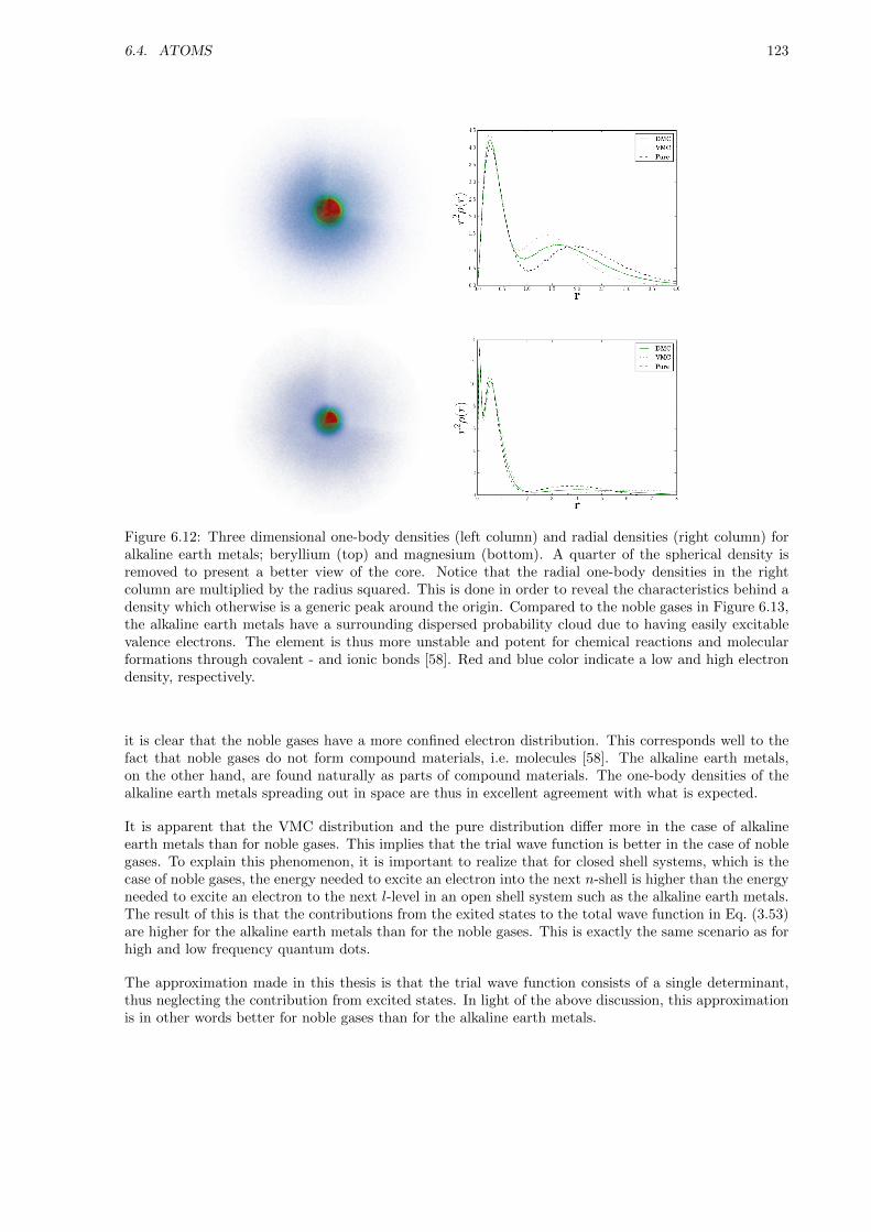
6.4. ATOMS 123
Figure 6.12: Three dimensional one-body densities (left column) and radial densities (right column) foralkaline earth metals; beryllium (top) and magnesium (bottom). A quarter of the spherical density isremoved to present a better view of the core. Notice that the radial one-body densities in the rightcolumn are multiplied by the radius squared. This is done in order to reveal the characteristics behind adensity which otherwise is a generic peak around the origin. Compared to the noble gases in Figure 6.13,the alkaline earth metals have a surrounding dispersed probability cloud due to having easily excitablevalence electrons. The element is thus more unstable and potent for chemical reactions and molecularformations through covalent - and ionic bonds [58]. Red and blue color indicate a low and high electrondensity, respectively.
it is clear that the noble gases have a more confined electron distribution. This corresponds well to thefact that noble gases do not form compound materials, i.e. molecules [58]. The alkaline earth metals,on the other hand, are found naturally as parts of compound materials. The one-body densities of thealkaline earth metals spreading out in space are thus in excellent agreement with what is expected.
It is apparent that the VMC distribution and the pure distribution differ more in the case of alkalineearth metals than for noble gases. This implies that the trial wave function is better in the case of noblegases. To explain this phenomenon, it is important to realize that for closed shell systems, which is thecase of noble gases, the energy needed to excite an electron into the next n-shell is higher than the energyneeded to excite an electron to the next l-level in an open shell system such as the alkaline earth metals.The result of this is that the contributions from the exited states to the total wave function in Eq. (3.53)are higher for the alkaline earth metals than for the noble gases. This is exactly the same scenario as forhigh and low frequency quantum dots.
The approximation made in this thesis is that the trial wave function consists of a single determinant,thus neglecting the contribution from excited states. In light of the above discussion, this approximationis in other words better for noble gases than for the alkaline earth metals.
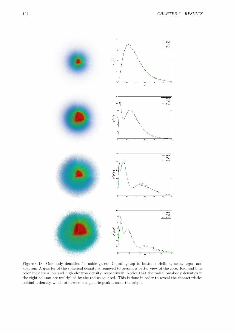
124 CHAPTER 6. RESULTS
Figure 6.13: One-body densities for noble gases. Counting top to bottom: Helium, neon, argon andkrypton. A quarter of the spherical density is removed to present a better view of the core. Red and bluecolor indicate a low and high electron density, respectively. Notice that the radial one-body densities inthe right column are multiplied by the radius squared. This is done in order to reveal the characteristicsbehind a density which otherwise is a generic peak around the origin.

6.5. HOMONUCLEAR DIATOMIC MOLECULES 125
Molecule R EVMC EDMC Expt. εrel
H2 1.4 -1.1551(3) -1.1745(3) −1.1746 8.51 · 10−5
Li2 5.051 -14.743(3) -14.988(2) −14.99544 4.96 · 10−4
Be2 4.63 -28.666(5) -29.301(5) −29.33854(5) 1.28 · 10−3
B2 3.005 -47.746(7) -49.155(5) −49.4184 5.33 · 10−3
C2 2.3481 -72.590(8) -74.95(1) −75.923(5) 1.28 · 10−2
N2 2.068 -102.78(1) -106.05(2) −109.5423 3.19 · 10−2
O2 2.282 -143.97(2) -148.53(2) −150.3268 1.2 · 10−2
Table 6.8: Ground state energies for homonuclear diatomic molecules calculated using VMC and DMC.The distance between the atoms R are taken from Ref. [3] for H2 and from Ref. [30] for Li2 to O2. Theexperimental energies, that is, the best possible results available, are taken from Ref. [3] for H2 and fromRef. [4] for Li2 to O2. As expected DMC is closer to the experimental energy than VMC. Moreover, therelative error εrel = |EDMC − Expt.|/|Expt.| is as expected lowest in the case of H2, and increases withatomic number.
6.5 Homonuclear Diatomic Molecules
The focus regarding homonuclear diatomic molecules, from here on referred to as molecules, has beensimilar to the focus on atoms, with the exception of parameterizing atomic force fields which can beapplied in molecular dynamics simulations. The implementation of molecular systems was achieved byadding ∼ 200 lines of code. This fact by itself represents a successful result regarding the code structure.As for atoms, the optimal calculations are referred to as experimental results. Details regarding thetransformation from atomic to molecular systems are given in Section 5.1.3.
6.5.1 Ground State Energies
Table 6.8 lists the VMC and DMC results with the corresponding experimental energies for H2 throughO2. As expected, the two-particle result is very close to the experimental value with the same precisionas the result for the helium atom in Table 6.7. The relative error from the experimental energy increaseswith atomic number, and is far higher than the errors in the case of pure atoms. This comes as a resultof the trial wave function being less optimal due to the fact that it does not account for the atomic nucleiinteraction term in the molecular Hamiltonian. Nevertheless, taking the simple nature of the trial wavefunction into consideration, the calculated energies are satisfyingly close to the experimental ones.
As with atoms, the energies were calculated on a single node, resulting in a rather big statistical errorin DMC. Doing the calculations on a supercomputer with an increase in the number of walkers shoulddecrease the errors.
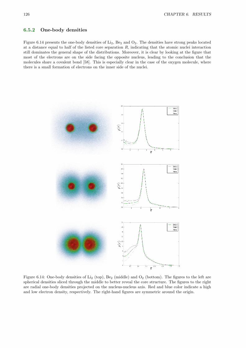
126 CHAPTER 6. RESULTS
6.5.2 One-body densities
Figure 6.14 presents the one-body densities of Li2, Be2 and O2. The densities have strong peaks locatedat a distance equal to half of the listed core separation R, indicating that the atomic nuclei interactionstill dominates the general shape of the distributions. Moreover, it is clear by looking at the figure thatmost of the electrons are on the side facing the opposite nucleus, leading to the conclusion that themolecules share a covalent bond [58]. This is especially clear in the case of the oxygen molecule, wherethere is a small formation of electrons on the inner side of the nuclei.
Figure 6.14: One-body densities of Li2 (top), Be2 (middle) and O2 (bottom). The figures to the left arespherical densities sliced through the middle to better reveal the core structure. The figures to the rightare radial one-body densities projected on the nucleus-nucleus axis. Red and blue color indicate a highand low electron density, respectively. The right-hand figures are symmetric around the origin.
6.5. HOMONUCLEAR DIATOMIC MOLECULES 127
6.5.3 Parameterizing Force Fields
In molecular dynamics, it is custom to use the Lennard Jones 12-6 potential as an ansatz to the interactionbetween pairs of atoms [10,11]
V (R) = 4ε
(( σR
)12
−( σR
)6), (6.4)
where ε and σ are parameters which can be fit to a given system.
However, the force field can be parameterized in greater detail using QMC calculations, resulting in amore precise molecular dynamics simulation [7]. The quantity of interest is the force, that is, the gradientof the potential. The classical potential in molecular dynamics does not correspond to the potential inthe Schrodinger equation, due to the fact that the kinetic energy contribution from the electrons is notcounted as part of the total kinetic energy in the molecular dynamics simulation. Hence it is the totalenergy of the Schrodinger equation which corresponds to the potential energy in molecular dynamics. Inthe case of diatomic molecules this means that
FMD =d〈E〉dR
. (6.5)
Expressions for this derivative can be obtained in ab-initio methods by using the Hellmann-Feynmantheorem [7]. However, the derivative can be approximated by the slope of the energy in Figure 6.15. Thefigure shows that there are clear similarities between the widely used Lennard-Jones 12-6 potential andthe results of QMC calculations done in this thesis, leading to the conclusion that the current state ofthe code can in fact produce approximations to atomic force fields for use in molecular dynamics.
For more complicated molecules, modelling the force using a single parameter R does not serve as a goodapproximation. However, the force can be found as a function of several angles, radii, etc., which in turncan be used to parameterize a more complicated molecular dynamics potential. An example of such apotential is the ReaxFF potential for hydrocarbons [59].

128 CHAPTER 6. RESULTS
(a) H2 (b) Li2
Figure 6.15: Top figures: The distance between the atoms R vs. the potential and total energy calculatedusing QMC. To the left: H2. To the right: Li2. It is evident that there exists a well-defined energyminimum in the case of hydrogen. For lithium this is not the case, which is expected since lithiumdoes not appear naturally in a diatomic gas phase, but rather as an ionic compound in other molecules[58]. Bottom figure: The general shape of the Lennard-Jones potential commonly used in moleculardynamics simulations as an approximation to the potential between atoms. The top figures clearlyresemble the Lennard-Jones 12-6 potential, leading to the conclusion that QMC calculations can be usedto parameterize a more realistic potential.
(c) The Lennard-Jones 12-6 potential with σ = ε = 1.
7
Conclusions
The focus of this thesis was to develop an efficient and general Quantum Monte-Carlo (QMC) solverwhich could simulate various systems with a large number of particles. This was achieved by usingobject oriented C++, resulting in ∼ 15000 lines of code. The code was redesigned a total of four times.The final structure was carefully planned in advance of the coding process. The linear algebra libraryArmadillo [60] was used in order to have a structured and easy code regarding all the matrices relatedto the walkers and the system in general.
It became apparent that in order to maintain efficiency for a high number of particles, closed formexpressions for the single-particle wave function derivatives were necessary. For two-dimensional quantumdots, 112 of these expressions were needed to simulate the 56-particle system. Needless to say, this processhad to be automated. This was achieved by using SymPy, an open source symbolic algebra package forPython, wrapped in a script which generated all the C++ necessary code within seconds. This task isdescribed in detail in Appendix C. A total of 252 expressions were generated.
As the solver became more and more flexible, the dire need of a control script arose. Hence the currentstate of the code is 100% controlled by a Python script. The script translates configuration files toinstructions which are fed to the pre-compiled C++ program. In addition, the script sets up the properenvironment for the simulation, that is, it makes sure the simulation output is stored in a folder stampedwith the current date and time, as well as with a supplied name tag. All in all, this made it possible torun an immense amount of different simulations without loosing track of the data.
In order to handle the increase in data, a script which automatically converted the output files to Latextables were written. However, this would not uncover whether or not the simulations had converged. Anadditional script was thus written, which made the process of visualizing immense amounts of data verysimple. Moreover, the data could be analyzed real-time, which meant that failing simulations could bedetected and aborted before they were complete, saving a lot of time. Expanding the script to handlenew output files was by design unproblematic. This script is covered in high detail in Appendix B.
Several Master projects over the years have involved QMC simulations of some sort, like VariationalMonte-Carlo (VMC) calculations of two-dimensional quantum dots up to 42 particles [28], and VMCcalculations of atoms up to Silicon (14 particles) [61]. In this thesis, the step was taken to full DiffusionMonte-Carlo (DMC) studies of both systems, adding three-dimensional - and double-well quantum dotsin addition to homonuclear diatomic molecules. Additionally, the simulation sizes were increased to 56electrons and krypton (36 particles) for two-dimensional quantum dots and atoms, respectively.
The optimization of the code was done by profiling the code, focusing on the parts which took the mosttime. Due to the general structure of the code, the function responsible for diffusing the particles wasresponsible for almost all of the run time. This function is at the core of Adaptive Stochastic Gradient
129
130 CHAPTER 7. CONCLUSIONS
Descent (ASGD), VMC and DMC. In other words, the task of optimization the full code decreased downto the task of optimizing this specific function. By optimizing one part of the diffusion process at thetime, the final run time was successfully reduced to 5% of the original.
Having successfully implemented five different systems demonstrates the code’s generality. The implemen-tation of molecules and the double-well was done by adding no more than 200 lines of code. Additionally,implementing three-dimensional quantum dots was done in an afternoon. Overall the code has lived upto every single one of the initial aims, with the exception of simulating bosons. Studying new fermionicsystems were considered more interesting, hence specific implementations for bosons were abandoned.
For quantum dots, both VMC and DMC perform very well. The results from Full Configuration Inter-action [8] for two particles, which are believed to be very close to the exact solution, are reproducedto five digits using DMC, with the VMC result being a little higher (2-3 digits). For atomic systems,the difference in results in VMC and DMC increase. This is expected since the trial wave function doesnot include the unbound states of the atoms. Nevertheless, DMC performs very well, reproducing theexperimental results for two particles with an error at the level of 10−4. For heavier atoms, the errorincreases somewhat, however, taking into consideration the simple trial wave function, the results areremarkably good.
Moreover, it was found that the radial distributions of two - and three-dimensional quantum dots with thesame number of closed shells were remarkably similar. This, however, is only the case at high frequencies.For lower frequencies, both systems were found to transition into Wigner crystallized states, however, thedistributions were no longer similar. This breaking of symmetry is an extremely interesting phenomenon,which can be studied in greater detail in order to say something general about how the number of spatialdimensions affect systems of confined electrons. The Wigner crystallization is covered in high detail inthe literature [49–53], however, a new approach using the virial theorem was investigated in order todescribe the transition.
It is clear that the energy of H2 graphed as a function of the core separation resembles the Lennard-Jones12-6 potential. This demonstrates that the code can be used to parameterize potential energies for use inmolecular dynamics simulations, however, to produce realistic potentials, support for more complicatedmolecules must be implemented.
Prospects and future work
Shortly after handing in this thesis, I will focus my effort on studying the relationship between two - andthree-dimensional quantum dots in higher detail. The goal is to publish my findings, and possibly saysomething general regarding how the number of dimensions affect a system of confined electrons.
Additionally, the double-well quantum dot will be studied in higher detail using realistic values for theparameters. These results can then be benchmarked with the results of Sigve Bøe Skattum and hisMulti-configuration Time Dependent Hartree-Fock solver [19].
My supervisor and I will at the same time work with implementing a momentum space version of QMC.This has the potential of describing nuclear interactions in great detail [62].
I will continue my academic career as a PhD student in the field of multi-scale physics. The transitionfrom QMC to molecular dynamics will thus be of high interest. The plan is to expand the code to generalmolecules. However, in order to maintain a reasonable precision, the single-particle wave functionsneed to be optimized. Hence implementing a Hartree-Fock solver [18] or using a Coupled Cluster wavefunction [63] will be prioritized.

Appendices
131

A
Dirac Notation
Calculations involving sums over inner products of orthogonal states are common in Quantum Mechanics.This due to the fact that eigenfunctions of Hermitian operators, which is the kind of operators whichrepresent observables [17], are necessarily orthogonal [31]. These inner-products will in many casesresult in either zero or one, i.e. the Kronecker-delta function δij ; explicitly calculating the integrals isunnecessary.
Dirac notation is a notation in which quantum states are represented as abstract components of a Hilbertspace, i.e. an inner product space. This implies that the inner-product between two states are representedby these states alone, without the integral over a specific basis, which makes derivations a lot cleaner andgeneral in the sense that no specific basis is needed.
Extracting the abstract state from a wave function is done by realizing that the wave function can bewritten as the inner product between the position basis eigenstates |x〉 and the abstract quantum state|ψ〉
ψ(x) = 〈r, ψ〉 ≡ 〈x|ψ〉 = 〈x| × |ψ〉 .
The notation is designed to be simple. The right hand side of the inner product is called a ket, while theleft hand side is called a bra. Combining both of them leaves you with an inner product bracket, henceDirac notation is commonly referred to as bra-ket notation.
To demonstrate the simplicity introduced with this notation, imagine a coupled two-level spin- 12 system
in the following state
|χ〉 = N[|↑↓〉 − i |↓↑〉
](A.1)
〈χ| = N[〈↑↓|+ i 〈↓↑|
](A.2)
Using the fact that both the |χ〉 state and the two-level spin states should be orthonormal, the normal-ization factor can be calculated without explicitly setting up any integrals
133
134 APPENDIX A. DIRAC NOTATION
〈χ|χ〉 = N2[〈↑↓|+ i 〈↓↑|
][|↑↓〉 − i |↓↑〉
]= N2
[〈↑↓ | ↑↓〉+ i 〈↓↑ | ↑↓〉 − i 〈↑↓ | ↓↑〉+ 〈↓↑ | ↓↑〉
]= N2
[1 + 0− 0 + 1
]= 2N2
= 1,
This implies the trivial solution N = 1/√
2. With this powerful notation at hand, important propertiessuch as the completeness relation of a set of states can be shown. A standard strategy is to start byexpanding one state |φ〉 in a complete set of different states |ψi〉:
|φ〉 =∑i
ci |ψi〉
〈ψk|φ〉 =∑i
ci 〈ψk|ψi〉︸ ︷︷ ︸δik
= ck
|φ〉 =∑i
〈ψi|φ〉 |ψi〉
=
[∑i
|ψi〉 〈ψi|
]|φ〉
which implies that
∑i
|ψi〉 〈ψi| = 1 (A.3)
for any complete set of orthonormal states |ψi〉. Calculating the corresponding identity for a continuousbasis like e.g. the position basis yields
∫|ψ(x)|2dx = 1 (A.4)∫|ψ(x)|2dx =
∫ψ∗(x)ψ(x)dx
=
∫〈ψ|x〉 〈x|ψ〉dx
= 〈ψ|[ ∫|x〉 〈x| dx
]|ψ〉 . (A.5)
Combining eq. A.4 and eq. A.5 with the fact that 〈ψ|ψ〉 = 1 yields the identity
∫|x〉 〈x| dx = 1. (A.6)
Looking back at the introductory example, this identity is exactly what is extracted when a wave functionis described as an inner product instead of an explicit function.
B
DCViz: Visualization of Data
With a code framework increasing in complexity comes an increasing need for tools to ease the interfacebetween the code and the developer(s). In computational science, a must-have tool is a tool for efficientvisualization of data; there is only so much information a single number can hold. To supplement theQMC code, a visualization tool named DCViz (Dynamic Column data Visualizer) has been developed.
The tool is written in Python, designed to plot data stored in columns. The tool is not designed explicitlyfor the QMC framework, and has been successfully applied to codes by several Master students at thetime of this thesis. The plot library used is Matplotlib [64] with a graphical user interface coded usingPySide [65]. The data can be plotted dynamically at a specified interval, and designed to be run parallelto the main application, e.g. DMC.
DCViz is available at https://github.com/jorgehog/DCViz
B.1 Basic Usage
The application is centered around the mainloop() function, which handles the extraction of data, thefigures and so on. The virtual function plot() is where the user specifies how the data is transformed intospecified figures by creating a subclass which overloads it. The superclass handles everything from safereading from dynamically changing files, efficient and safe re-plotting of data, etc. automatically. Thetool is designed to be simple to use by having a minimalistic interface for implementing new visualizationclasses. The only necessary members to specify in a new implementation is described in the first threesections, from where the remaining sections will cover additional support.
The figure map
Represented by the member variable figMap, the figure map is where the user specifies the figure setup,that is, the names of the main-figures and their sub-figures. Consider the following figure map:
1 figMap = {"mainFig1": ["subFig1", "subFig2"], "mainFig2": []}
This would cause DCViz to create two main-figures self.mainFig1 and self.mainFig2, which can beaccessed in the plot function. Moreover, the first main-figure will contain two sub-figures accessiblethrough self.subFig1 and self.subFig2. These sub-figures will be stacked vertically if not stack="H"is specified, in which they will be stacked horizontally.
135
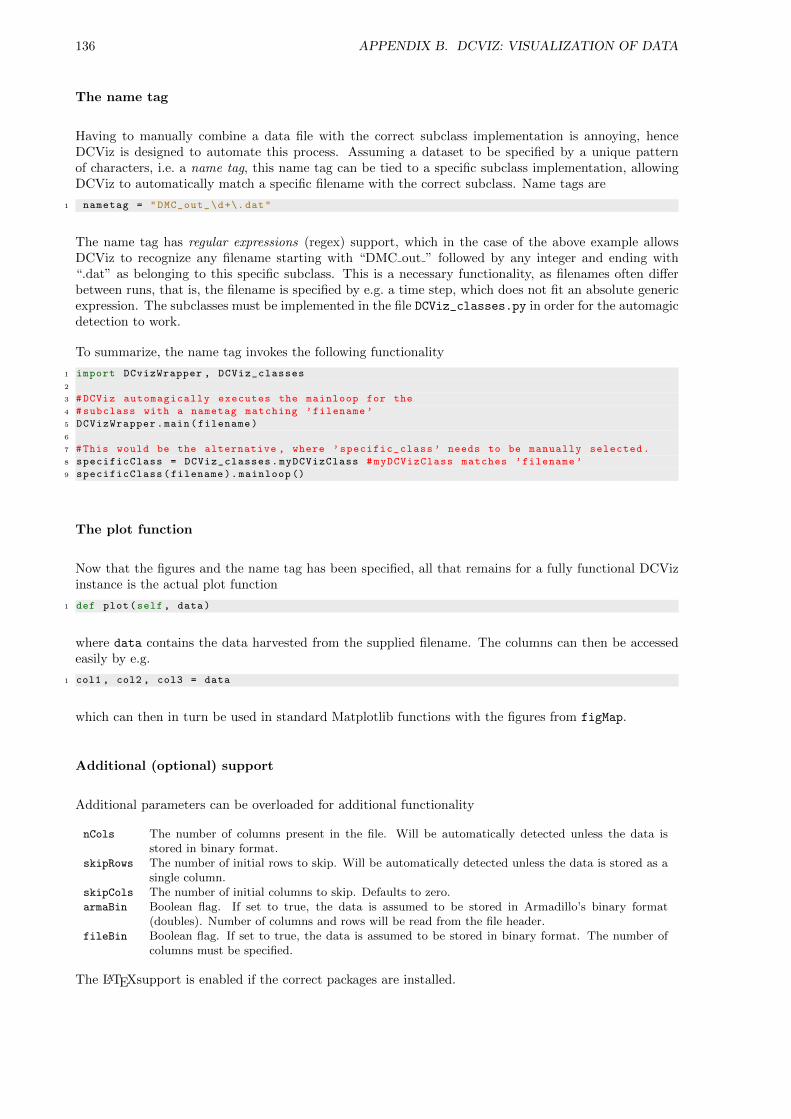
136 APPENDIX B. DCVIZ: VISUALIZATION OF DATA
The name tag
Having to manually combine a data file with the correct subclass implementation is annoying, henceDCViz is designed to automate this process. Assuming a dataset to be specified by a unique patternof characters, i.e. a name tag, this name tag can be tied to a specific subclass implementation, allowingDCViz to automatically match a specific filename with the correct subclass. Name tags are
1 nametag = "DMC_out_\d+\.dat"
The name tag has regular expressions (regex) support, which in the case of the above example allowsDCViz to recognize any filename starting with “DMC out ” followed by any integer and ending with“.dat” as belonging to this specific subclass. This is a necessary functionality, as filenames often differbetween runs, that is, the filename is specified by e.g. a time step, which does not fit an absolute genericexpression. The subclasses must be implemented in the file DCViz_classes.py in order for the automagicdetection to work.
To summarize, the name tag invokes the following functionality
1 import DCvizWrapper , DCViz_classes
2
3 #DCViz automagically executes the mainloop for the
4 #subclass with a nametag matching ’filename ’
5 DCVizWrapper.main(filename)
6
7 #This would be the alternative , where ’specific_class ’ needs to be manually selected.
8 specificClass = DCViz_classes.myDCVizClass #myDCVizClass matches ’filename ’
9 specificClass(filename).mainloop ()
The plot function
Now that the figures and the name tag has been specified, all that remains for a fully functional DCVizinstance is the actual plot function
1 def plot(self, data)
where data contains the data harvested from the supplied filename. The columns can then be accessedeasily by e.g.
1 col1 , col2 , col3 = data
which can then in turn be used in standard Matplotlib functions with the figures from figMap.
Additional (optional) support
Additional parameters can be overloaded for additional functionality
nCols The number of columns present in the file. Will be automatically detected unless the data isstored in binary format.
skipRows The number of initial rows to skip. Will be automatically detected unless the data is stored as asingle column.
skipCols The number of initial columns to skip. Defaults to zero.armaBin Boolean flag. If set to true, the data is assumed to be stored in Armadillo’s binary format
(doubles). Number of columns and rows will be read from the file header.fileBin Boolean flag. If set to true, the data is assumed to be stored in binary format. The number of
columns must be specified.
The LATEXsupport is enabled if the correct packages are installed.

B.1. BASIC USAGE 137
An example
1 #DCViz_classes.py
2
3 from DCViz_sup import DCVizPlotter #Import the superclass
4
5 class myTestClass(DCVizPlotter): #Create a new subclass
6 nametag = ’testcase\d\.dat’ #filename with regex support
7
8 #1 figure with 1 subfigure
9 figMap = {’fig1’: [’subfig1 ’]}
10
11 #skip first row (must be supplied since the data is 1D).
12 skipRows = 1
13
14 def plot(self, data):
15 column1 = data [0]
16
17 self.subfig1.set_title(’I have $\LaTeX$ support!’)
18
19 self.subfig1.set_ylim ([-1,1])
20
21 self.subfig1.plot(column1)
22
23 #exit function
Families
A specific implementation can be flagged as belonging to a family of similar files, that is, files in the samedirectory matching the same name tag. Flagging a specific DCViz subclass as a family is achieved bysetting the class member variable isFamilyMember to true. When a family class is initialized with a file,DCViz scans the file’s folder for additional matches to this specific class. If several matches are found,all of these are loaded into the data object given as input to the plot function. In this case data[i]
contains the column data of file i.
To keep track of which file a given data-set was loaded from, a list self.familyFileNames is created,where element i is the filename corresponding to data[i]. To demonstrate this, consider the followingexample
1 isFamilyMember = True
2 def plot(self, data)
3
4 file1 , file2 = data
5 fileName1 , fileName2 = self.familyFileNames
6
7 col1_1 , col_2_1 = file1
8 col1_2 , col_2_2 = file2
9 #...
A class member string familyName can be overridden to display a more general name in the auto-detectionfeedback.
Families are an important functionality in the cases where the necessary data is spread across several files.For instance, in the QMC library, the radial distributions of both VMC and DMC are needed in order togenerate the plots shown in Figure 6.6 of the results chapter. These results may be generated in separateruns, which implies that they either needs to be loaded as a family, or be concatenated beforehand.Which dataset belongs to VMC and DMC can be extracted from the list of family file names.
All the previous mentioned functionality is available for families.

138 APPENDIX B. DCVIZ: VISUALIZATION OF DATA
Family example
1 #DCViz_classes.py
2
3 from DCViz_sup import DCVizPlotter
4
5 class myTestClassFamily(DCVizPlotter):
6 nametag = ’testcaseFamily\d\.dat’ #filename with regex support
7
8 #1 figure with 3 subfigures
9 figMap = {’fig1’: [’subfig1 ’, ’subfig2 ’, ’subfig3 ’]}
10
11 #skip first row of each data file.
12 skipRows = 1
13
14 #Using this flag will read all the files matching the nametag
15 #(in the same folder .) and make them aviable in the data arg
16 isFamilyMember = True
17 familyName = "testcase"
18
19 def plot(self, data):
20
21 mainFig = self.fig1
22 mainFig.suptitle(’I have $\LaTeX$ support!’)
23 subfigs = [self.subfig1 , self.subfig2 , self.subfig3]
24
25 #Notice that fileData.data is plotted (the numpy matrix of the columns)
26 #and not fileData alone , as fileData is a ’dataGenerator ’ instance
27 #used to speed up file reading. Alternatively , data [:] could be sent
28 for subfig , fileData in zip(subfigs , data):
29 subfig.plot(fileData.data)
30 subfig.set_ylim ([-1,1])
loading e.g. testcaseFamily0.dat would automatically load testcaseFamily1.dat etc. as well.
Dynamic mode
Dynamic mode in DCViz is enabled on construction of the object
1 DCVizObj = myDCVizClass(filename , dynamic=True)
2 DCVizObj.mainloop ()
This flag lets the mainloop know that it should not stop after the initial plot is generated, but rather keepon reading and plotting the file(s) until the user ends the loop with either a keyboard-interrupt (whichis caught and safely handled), or in the case of using the GUI, with the stop button.
In order to make this functionality more CPU-friendly, a delay parameter can be adjusted to specify apause period in between re-plotting.
Saving figures to file
The generated figures can be saved to file by passing a flag to the constructor
1 DCVizObj = myDCVizClass(filename , toFile=True)
2 DCVizObj.mainloop ()
In this case, dynamic mode is disabled and the figures will not be drawn on screen, but rather saved ina subfolder of the supplied filename’s folder called DCViz_out.
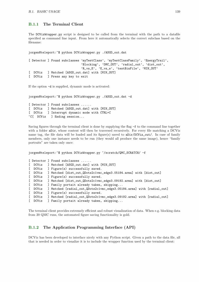
B.1. BASIC USAGE 139
B.1.1 The Terminal Client
The DCVizWrapper.py script is designed to be called from the terminal with the path to a datafilespecified as command line input. From here it automatically selects the correct subclass based on thefilename:
jorgen@teleport:~$ python DCVizWrapper.py ./ASGD_out.dat
[ Detector ] Found subclasses ’myTestClass’, ’myTestClassFamily’, ’EnergyTrail’,
’Blocking’, ’DMC_OUT’, ’radial_out’, ’dist_out’,
’R_vs_E’, ’E_vs_w’, ’testBinFile’, ’MIN_OUT’
[ DCViz ] Matched [ASGD_out.dat] with [MIN_OUT]
[ DCViz ] Press any key to exit
If the option -d is supplied, dynamic mode is activated:
jorgen@teleport:~$ python DCVizWrapper.py ./ASGD_out.dat -d
[ Detector ] Found subclasses ......
[ DCViz ] Matched [ASGD_out.dat] with [MIN_OUT]
[ DCViz ] Interrupt dynamic mode with CTRL+C
^C[ DCViz ] Ending session...
Saving figures through the terminal client is done by supplying the flag -f to the command line togetherwith a folder aDir, whose content will then be traversed recursively. For every file matching a DCVizname tag, the file data will be loaded and its figure(s) saved to aDir/DCViz_out/. In case of familymembers, only one instance needs to be run (they would all produce the same image), hence “familyportraits” are taken only once:
jorgen@teleport:~$ python DCVizWrapper.py ~/scratch/QMC_SCRATCH/ -f
[ Detector ] Found subclasses ......
[ DCViz ] Matched [ASGD_out.dat] with [MIN_OUT]
[ DCViz ] Figure(s) successfully saved.
[ DCViz ] Matched [dist_out_QDots2c1vmc_edge3.05184.arma] with [dist_out]
[ DCViz ] Figure(s) successfully saved.
[ DCViz ] Matched [dist_out_QDots2c1vmc_edge3.09192.arma] with [dist_out]
[ DCViz ] Family portait already taken, skipping...
[ DCViz ] Matched [radial_out_QDots2c1vmc_edge3.05184.arma] with [radial_out]
[ DCViz ] Figure(s) successfully saved.
[ DCViz ] Matched [radial_out_QDots2c1vmc_edge3.09192.arma] with [radial_out]
[ DCViz ] Family portait already taken, skipping...
The terminal client provides extremely efficient and robust visualization of data. When e.g. blocking datafrom 20 QMC runs, the automated figure saving functionality is gold.
B.1.2 The Application Programming Interface (API)
DCViz has been developed to interface nicely with any Python script. Given a path to the data file, allthat is needed in order to visualize it is to include the wrapper function used by the terminal client:
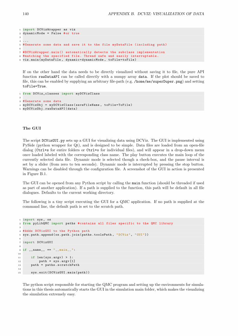
140 APPENDIX B. DCVIZ: VISUALIZATION OF DATA
1 import DCVizWrapper as viz
2 dynamicMode = False #or true
3
4 ...
5 #Generate some data and save it to the file myDataFile (including path)
6
7 #DCVizWrapper.main() automatically detects the subclass implementation
8 #matching the specified file. Thread safe and easily interruptable.
9 viz.main(myDataFile , dynamic=dynamicMode , toFile=toFile)
If on the other hand the data needs to be directly visualized without saving it to file, the pure APIfunction rawDataAPI can be called directly with a numpy array data. If the plot should be saved tofile, this can be enabled by supplying an arbitrary file-path (e.g. /home/me/superDuper.png) and settingtoFile=True.
1 from DCViz_classes import myDCVizClass
2
3 #Generate some data
4 myDCVizObj = myDCVizClass(saveFileName , toFile=ToFile)
5 myDCVizObj.rawDataAPI(data)
The GUI
The script DCVizGUI.py sets up a GUI for visualizing data using DCViz. The GUI is implemented usingPySide (python wrapper for Qt), and is designed to be simple. Data files are loaded from an open-filedialog (Ctrl+s for entire folders or Ctrl+o for individual files), and will appear in a drop-down menuonce loaded labeled with the corresponding class name. The play button executes the main loop of thecurrently selected data file. Dynamic mode is selected though a check-box, and the pause interval isset by a slider (from zero to ten seconds). Dynamic mode is interrupted by pressing the stop button.Warnings can be disabled through the configuration file. A screenshot of the GUI in action is presentedin Figure B.1.
The GUI can be opened from any Python script by calling the main function (should be threaded if usedas part of another application). If a path is supplied to the function, this path will be default in all filedialogues. Defaults to the current working directory.
The following is a tiny script executing the GUI for a QMC application. If no path is supplied at thecommand line, the default path is set to the scratch path.
1 import sys , os
2 from pyLibQMC import paths #contains all files specific to the QMC library
3
4 #Adds DCVizGUI to the Python path
5 sys.path.append(os.path.join(paths.toolsPath , "DCViz", "GUI"))
6
7 import DCVizGUI
8
9 if __name__ == "__main__":
10
11 if len(sys.argv) > 1:
12 path = sys.argv [1]
13 path = paths.scratchPath
14
15 sys.exit(DCVizGUI.main(path))
The python script responsible for starting the QMC program and setting up the environments for simula-tions in this thesis automatically starts the GUI in the simulation main folder, which makes the visualizingthe simulation extremely easy.

B.1. BASIC USAGE 141
Figure B.1: Two consequent screen shots of the GUI. The first (top) is taken directly after the detectoris finished loading files into the drop-down menu. The second is taken directly after the job is started.
Alternatively, DCVizGUI.py can be executed directly from the terminal with an optional default path asfirst command line argument.
The following is the terminal feedback supplied from opening the GUI
.../DCViz/GUI$ python DCVizGUI.py
[ Detector ]: Found subclasses ’myTestClass’, ’myTestClassFamily’, ’EnergyTrail’,
’Blocking’, ’DMC_OUT’, ’radial_out’, ’dist_out’, ’testBinFile’, ’MIN_OUT’
[ GUI ]: Data reset.
Selecting a folder from the open-folder dialog initializes the detector on all file content
[ Detector ]: matched [ DMC_out.dat ] with [ DMC_OUT ]
[ Detector ]: matched [ ASGD_out.dat ] with [ MIN_OUT ]
[ Detector ]: matched [blocking_DMC_out.dat] with [ Blocking ]
[ Detector ]: ’blocking_MIN_out0_RAWDATA.arma’ does not match any DCViz class
[ Detector ]: ’blocking_DMC_out_RAWDATA.arma’ does not match any DCViz class
[ Detector ]: matched [blocking_VMC_out.dat] with [ Blocking ]
Executing a specific file selected from the drop-down menu starts a threaded job, hence several non-dynamic jobs can be ran at once. The limit is set to one dynamic job pr. application due to the highCPU cost (in case of a low pause timer).
The terminal output can be silenced through to configuration file to not interfere with the standardoutput of an application. Alternatively, the GUI thread can redirect its standard output to file.

142
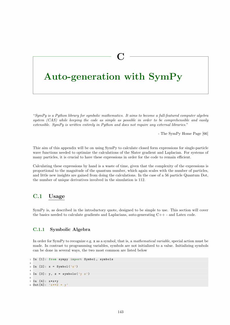
C
Auto-generation with SymPy
“SymPy is a Python library for symbolic mathematics. It aims to become a full-featured computer algebrasystem (CAS) while keeping the code as simple as possible in order to be comprehensible and easilyextensible. SymPy is written entirely in Python and does not require any external libraries.”
- The SymPy Home Page [66]
Thie aim of this appendix will be on using SymPy to calculate closed form expressions for single-particlewave functions needed to optimize the calculations of the Slater gradient and Laplacian. For systems ofmany particles, it is crucial to have these expressions in order for the code to remain efficient.
Calculating these expressions by hand is a waste of time, given that the complexity of the expressions isproportional to the magnitude of the quantum number, which again scales with the number of particles,and little new insights are gained from doing the calculations. In the case of a 56 particle Quantum Dot,the number of unique derivatives involved in the simulation is 112.
C.1 Usage
SymPy is, as described in the introductory quote, designed to be simple to use. This section will coverthe basics needed to calculate gradients and Laplacians, auto-generating C++ - and Latex code.
C.1.1 Symbolic Algebra
In order for SymPy to recognize e.g. x as a symbol, that is, a mathematical variable, special action must bemade. In contrast to programming variables, symbols are not initialized to a value. Initializing symbolscan be done in several ways, the two most common are listed below
1 In [1]: from sympy import Symbol , symbols
2
3 In [2]: x = Symbol(’x’)
4
5 In [3]: y, z = symbols(’y z’)
6
7 In [4]: x*x+y
8 Out [4]: ’x**2 + y’
143
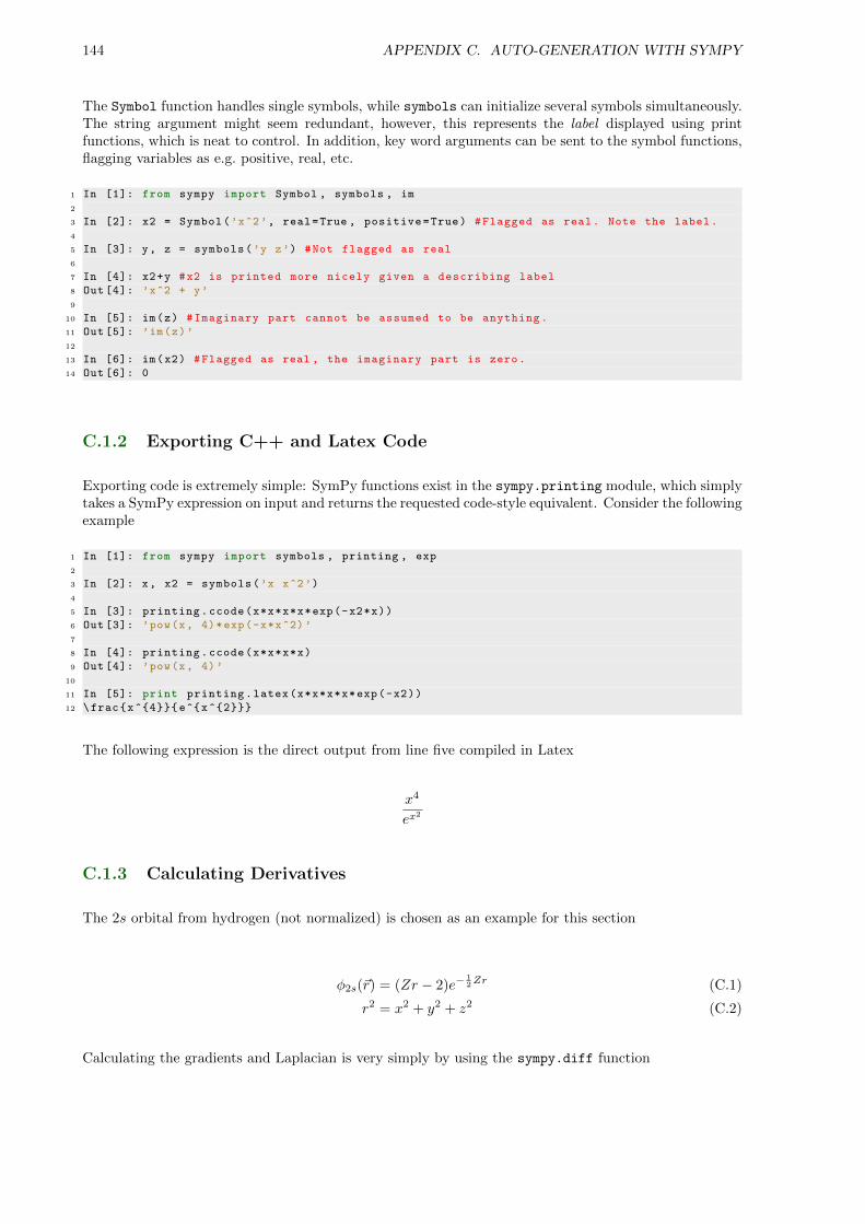
144 APPENDIX C. AUTO-GENERATION WITH SYMPY
The Symbol function handles single symbols, while symbols can initialize several symbols simultaneously.The string argument might seem redundant, however, this represents the label displayed using printfunctions, which is neat to control. In addition, key word arguments can be sent to the symbol functions,flagging variables as e.g. positive, real, etc.
1 In [1]: from sympy import Symbol , symbols , im
2
3 In [2]: x2 = Symbol(’x^2’, real=True , positive=True) #Flagged as real. Note the label.
4
5 In [3]: y, z = symbols(’y z’) #Not flagged as real
6
7 In [4]: x2+y #x2 is printed more nicely given a describing label
8 Out [4]: ’x^2 + y’
9
10 In [5]: im(z) #Imaginary part cannot be assumed to be anything.
11 Out [5]: ’im(z)’
12
13 In [6]: im(x2) #Flagged as real , the imaginary part is zero.
14 Out [6]: 0
C.1.2 Exporting C++ and Latex Code
Exporting code is extremely simple: SymPy functions exist in the sympy.printing module, which simplytakes a SymPy expression on input and returns the requested code-style equivalent. Consider the followingexample
1 In [1]: from sympy import symbols , printing , exp
2
3 In [2]: x, x2 = symbols(’x x^2’)
4
5 In [3]: printing.ccode(x*x*x*x*exp(-x2*x))
6 Out [3]: ’pow(x, 4)*exp(-x*x^2)’
7
8 In [4]: printing.ccode(x*x*x*x)
9 Out [4]: ’pow(x, 4)’
10
11 In [5]: print printing.latex(x*x*x*x*exp(-x2))
12 \frac{x^{4}}{e^{x^{2}}}
The following expression is the direct output from line five compiled in Latex
x4
ex2
C.1.3 Calculating Derivatives
The 2s orbital from hydrogen (not normalized) is chosen as an example for this section
φ2s(~r) = (Zr − 2)e−12Zr (C.1)
r2 = x2 + y2 + z2 (C.2)
Calculating the gradients and Laplacian is very simply by using the sympy.diff function
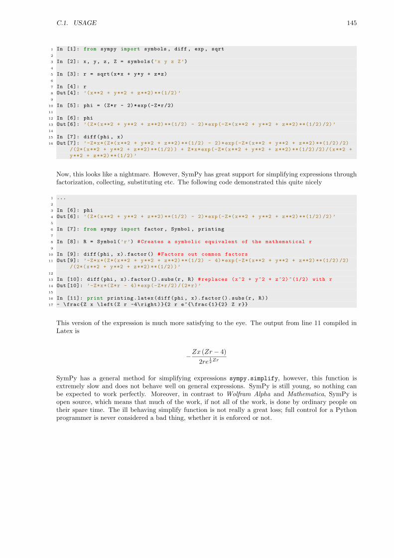
C.1. USAGE 145
1 In [1]: from sympy import symbols , diff , exp , sqrt
2
3 In [2]: x, y, z, Z = symbols(’x y z Z’)
4
5 In [3]: r = sqrt(x*x + y*y + z*z)
6
7 In [4]: r
8 Out [4]: ’(x**2 + y**2 + z**2) **(1/2) ’
9
10 In [5]: phi = (Z*r - 2)*exp(-Z*r/2)
11
12 In [6]: phi
13 Out [6]: ’(Z*(x**2 + y**2 + z**2) **(1/2) - 2)*exp(-Z*(x**2 + y**2 + z**2) **(1/2) /2)’
14
15 In [7]: diff(phi , x)
16 Out [7]: ’-Z*x*(Z*(x**2 + y**2 + z**2) **(1/2) - 2)*exp(-Z*(x**2 + y**2 + z**2) **(1/2) /2)
/(2*(x**2 + y**2 + z**2) **(1/2)) + Z*x*exp(-Z*(x**2 + y**2 + z**2) **(1/2) /2)/(x**2 +
y**2 + z**2) **(1/2) ’
Now, this looks like a nightmare. However, SymPy has great support for simplifying expressions throughfactorization, collecting, substituting etc. The following code demonstrated this quite nicely
1 ...
2
3 In [6]: phi
4 Out [6]: ’(Z*(x**2 + y**2 + z**2) **(1/2) - 2)*exp(-Z*(x**2 + y**2 + z**2) **(1/2) /2)’
5
6 In [7]: from sympy import factor , Symbol , printing
7
8 In [8]: R = Symbol(’r’) #Creates a symbolic equivalent of the mathematical r
9
10 In [9]: diff(phi , x).factor () #Factors out common factors
11 Out [9]: ’-Z*x*(Z*(x**2 + y**2 + z**2) **(1/2) - 4)*exp(-Z*(x**2 + y**2 + z**2) **(1/2) /2)
/(2*(x**2 + y**2 + z**2) **(1/2))’
12
13 In [10]: diff(phi , x).factor ().subs(r, R) #replaces (x^2 + y^2 + z^2) ^(1/2) with r
14 Out [10]: ’-Z*x*(Z*r - 4)*exp(-Z*r/2) /(2*r)’
15
16 In [11]: print printing.latex(diff(phi , x).factor ().subs(r, R))
17 - \frac{Z x \left(Z r -4\right)}{2 r e^{\ frac {1}{2} Z r}}
This version of the expression is much more satisfying to the eye. The output from line 11 compiled inLatex is
−Zx (Zr − 4)
2re12Zr
SymPy has a general method for simplifying expressions sympy.simplify, however, this function isextremely slow and does not behave well on general expressions. SymPy is still young, so nothing canbe expected to work perfectly. Moreover, in contrast to Wolfram Alpha and Mathematica, SymPy isopen source, which means that much of the work, if not all of the work, is done by ordinary people ontheir spare time. The ill behaving simplify function is not really a great loss; full control for a Pythonprogrammer is never considered a bad thing, whether it is enforced or not.

146 APPENDIX C. AUTO-GENERATION WITH SYMPY
Estimating the Laplacian is just a matter of summing double derivatives
1 ...
2
3 In [12]: (diff(diff(phi , x), x) +
4 ....: diff(diff(phi , y), y) +
5 ....: diff(diff(phi , z), z)).factor ().subs(r, R)
6 Out [12]: ’Z*(Z**2*x**2 + Z**2*y**2 + Z**2*z**2 - 10*Z*r + 16)*exp(-Z*r/2) /(4*r)’
7
8 In [13]: (diff(diff(phi , x), x) + #Not quite satisfying.
9 ....: diff(diff(phi , y), y) + #Let’s collect the ’Z’ terms.
10 ....: diff(diff(phi , z), z)).factor ().collect(Z).subs(r, R)
11 Out [13]: ’Z*(Z**2*(x**2 + y**2 + z**2) - 10*Z*r + 16)*exp(-Z*r/2) /(4*r)’
12
13 In [14]: (diff(diff(phi , x), x) + #Still not satisfying.
14 ....: diff(diff(phi , y), y) + #The r^2 terms needs to be substituted as well.
15 ....: diff(diff(phi , z), z)).factor ().collect(Z).subs(r, R).subs(r**2, R**2)
16 Out [14]: ’Z*(Z**2*r**2 - 10*Z*r + 16)*exp(-Z*r/2) /(4*r)’
17
18 In [15]: (diff(diff(phi , x), x) + #Let’s try to factorize once more.
19 ....: diff(diff(phi , y), y) +
20 ....: diff(diff(phi , z), z)).factor ().collect(Z).subs(r, R).subs(r**2, R**2).factor ()
21 Out [15]: ’Z*(Z*r - 8)*(Z*r - 2)*exp(-Z*r/2) /(4*r)’
Getting the right factorization may come across as tricky, but with minimal training this poses no realproblems.
C.2 Using the auto-generation Script
The superclass orbitalsGenerator aims to serve as an interface with the QMC C++ BasisFunctions
class, automatically generating the C++ code containing all the implementations of the derivatives forthe given single-particle states. The single-particle states are implemented in the generator by subclassesoverloading system specific virtual functions which will be described in the following sections.
C.2.1 Generating Latex code
The following methods are user-implemented functions used to calculate the expressions which are in turnautomagically converted to Latex code. Once they are implemented, the following code can be executedin order to create the latex output
1 orbitalSet = HO_3D.HOOrbitals3D(N=40) #Creating a 3D harm. osc. object
2 orbitalSet.closedFormify ()
3 orbitalSet.TeXToFile(outPath)
The constructor
The superclass constructor takes on input the maximum number of particles for which expressions shouldbe generated and the name of the orbital set, e.g. hydrogenic. Calling a superclass constructor from asubclass constructor is done in the following way
1 class hydrogenicOrbitals(orbitalGenerator):
2
3 def __init__(self, N):
4
5 super(hydrogenicOrbitals , self).__init__(N, "hydrogenic")
6 #...
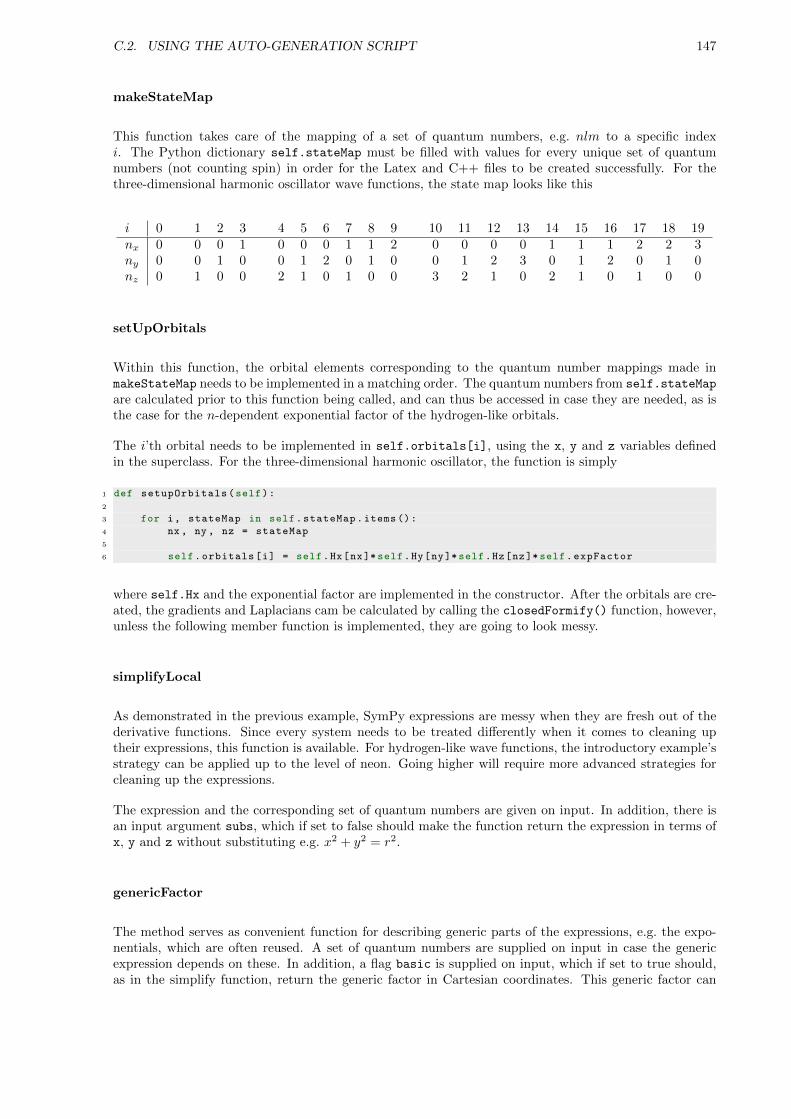
C.2. USING THE AUTO-GENERATION SCRIPT 147
makeStateMap
This function takes care of the mapping of a set of quantum numbers, e.g. nlm to a specific indexi. The Python dictionary self.stateMap must be filled with values for every unique set of quantumnumbers (not counting spin) in order for the Latex and C++ files to be created successfully. For thethree-dimensional harmonic oscillator wave functions, the state map looks like this
i 0 1 2 3 4 5 6 7 8 9 10 11 12 13 14 15 16 17 18 19nx 0 0 0 1 0 0 0 1 1 2 0 0 0 0 1 1 1 2 2 3ny 0 0 1 0 0 1 2 0 1 0 0 1 2 3 0 1 2 0 1 0nz 0 1 0 0 2 1 0 1 0 0 3 2 1 0 2 1 0 1 0 0
setUpOrbitals
Within this function, the orbital elements corresponding to the quantum number mappings made inmakeStateMap needs to be implemented in a matching order. The quantum numbers from self.stateMap
are calculated prior to this function being called, and can thus be accessed in case they are needed, as isthe case for the n-dependent exponential factor of the hydrogen-like orbitals.
The i’th orbital needs to be implemented in self.orbitals[i], using the x, y and z variables definedin the superclass. For the three-dimensional harmonic oscillator, the function is simply
1 def setupOrbitals(self):
2
3 for i, stateMap in self.stateMap.items():
4 nx, ny , nz = stateMap
5
6 self.orbitals[i] = self.Hx[nx]*self.Hy[ny]*self.Hz[nz]*self.expFactor
where self.Hx and the exponential factor are implemented in the constructor. After the orbitals are cre-ated, the gradients and Laplacians cam be calculated by calling the closedFormify() function, however,unless the following member function is implemented, they are going to look messy.
simplifyLocal
As demonstrated in the previous example, SymPy expressions are messy when they are fresh out of thederivative functions. Since every system needs to be treated differently when it comes to cleaning uptheir expressions, this function is available. For hydrogen-like wave functions, the introductory example’sstrategy can be applied up to the level of neon. Going higher will require more advanced strategies forcleaning up the expressions.
The expression and the corresponding set of quantum numbers are given on input. In addition, there isan input argument subs, which if set to false should make the function return the expression in terms ofx, y and z without substituting e.g. x2 + y2 = r2.
genericFactor
The method serves as convenient function for describing generic parts of the expressions, e.g. the expo-nentials, which are often reused. A set of quantum numbers are supplied on input in case the genericexpression depends on these. In addition, a flag basic is supplied on input, which if set to true should,as in the simplify function, return the generic factor in Cartesian coordinates. This generic factor can
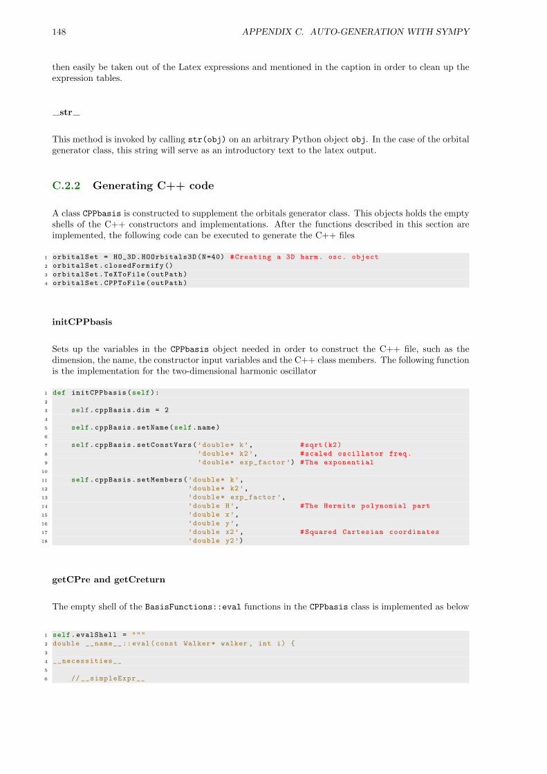
148 APPENDIX C. AUTO-GENERATION WITH SYMPY
then easily be taken out of the Latex expressions and mentioned in the caption in order to clean up theexpression tables.
str
This method is invoked by calling str(obj) on an arbitrary Python object obj. In the case of the orbitalgenerator class, this string will serve as an introductory text to the latex output.
C.2.2 Generating C++ code
A class CPPbasis is constructed to supplement the orbitals generator class. This objects holds the emptyshells of the C++ constructors and implementations. After the functions described in this section areimplemented, the following code can be executed to generate the C++ files
1 orbitalSet = HO_3D.HOOrbitals3D(N=40) #Creating a 3D harm. osc. object
2 orbitalSet.closedFormify ()
3 orbitalSet.TeXToFile(outPath)
4 orbitalSet.CPPToFile(outPath)
initCPPbasis
Sets up the variables in the CPPbasis object needed in order to construct the C++ file, such as thedimension, the name, the constructor input variables and the C++ class members. The following functionis the implementation for the two-dimensional harmonic oscillator
1 def initCPPbasis(self):
2
3 self.cppBasis.dim = 2
4
5 self.cppBasis.setName(self.name)
6
7 self.cppBasis.setConstVars(’double* k’, #sqrt(k2)
8 ’double* k2’, #scaled oscillator freq.
9 ’double* exp_factor ’) #The exponential
10
11 self.cppBasis.setMembers(’double* k’,
12 ’double* k2’,
13 ’double* exp_factor ’,
14 ’double H’, #The Hermite polynomial part
15 ’double x’,
16 ’double y’,
17 ’double x2’, #Squared Cartesian coordinates
18 ’double y2’)
getCPre and getCreturn
The empty shell of the BasisFunctions::eval functions in the CPPbasis class is implemented as below
1 self.evalShell = """
2 double __name__ ::eval(const Walker* walker , int i) {
3
4 __necessities__
5
6 // __simpleExpr__

C.2. USING THE AUTO-GENERATION SCRIPT 149
7
8 __preCalc__
9 return __return__
10
11 }
12 """
where __preCalc__ is a generated C++ expression returned from getCpre(), and __return__ is thereturned C++ expression from getCreturn(). The commented __simpleExpr__ will be replaced by theexpression in nicely formatted SymPy output code. __necessities__ is automatically detected by thescript, and represents the Cartesian variable expressions needed by the expressions.
The functions take a SymPy generated expression on input, i.e. an orbital, gradient or Laplacian, andthe corresponding index of the expression i. The reason these functions are split into a precalculationand a return expression is purely cosmetic. Consider the following example output for the hydrogen-likewave functions:
1 double dell_hydrogenic_9_y ::eval(const Walker* walker , int i) {
2
3 y = walker ->r(i, 1);
4 z = walker ->r(i, 2);
5
6 z2 = z*z;
7
8 //-y*(k*(-r^2 + 3*z^2) + 6*r)*exp(-k*r/3) /(3*r)
9
10 psi = -y*((*k)*(-walker ->get_r_i2(i) + 3*z2) + 6*walker ->get_r_i(i))/(3* walker ->
get_r_i(i));
11 return psi*(* exp_factor);
12
13 }
The *exp_factor is the precalculated n = 3 exponential which is then simply multiplied by the non-exponential terms before being returned. The commented line is a clean version of the full expression.The required Cartesian components are retrieved prior to the evaluation.
The full implementation of getCpre() and getCreturn() for the hydrogen-like wave functions are givenbelow
1 def getCReturn(self, expr , i):
2 return "psi*(* exp_factor);"
3
4 def getCPre(self, expr , i):
5 qNums = self.stateMap[i]
6 return " psi = %s;" % printing.ccode(expr/self.genericFactor(qNums))
makeOrbConstArg
Loading the generated BasisFunctions objects into the Orbitals object in the QMC code is rathera dull job, and is not designed to be done manually. The function makeOrbConstArg is designed toautomate this process. This is best demonstrated by an example: Consider the following constructor ofthe hydrogen-like wave function’s orbital class
1 basis_functions [0] = new hydrogenic_0(k, k2, exp_factor_n1);
2 basis_functions [1] = new hydrogenic_1(k, k2, exp_factor_n2);
3 //...
4 basis_functions [5] = new hydrogenic_5(k, k2, exp_factor_n3);
5 //..

150 APPENDIX C. AUTO-GENERATION WITH SYMPY
6 basis_functions [14] = new hydrogenic_14(k, k2, exp_factor_n4);
7 //..
8 basis_functions [17] = new hydrogenic_17(k, k2, exp_factor_n4);
where exp_factor_nk represents exp(−Zr/k), which is saved as a pointer reference for reasons explainedin Section 4.6.4. The same procedure is applied to the gradients and the Laplacians as well, leaving atotal of 90 sequential initializations. Everything needed in order to auto-generate the code is the followingimplementation
1 def makeOrbConstArgs(self, args , i):
2 n = self.stateMap[i][0]
3 args = args.replace(’exp_factor ’, ’exp_fa -ctor_n%d’ % n)
4 return args
which ensures that the input arguments to e.g. element 1 is (k, k2, exp_factor_n2), since the single-particle orbital self.phi[1] has a principle quantum number n = 2. The input argument args is thedefault constructor arguments set up the the initCPPbasis, and is in the case of hydrogen-like wavefunctions (k, k2, exp_factor).
The tables listed in Appendix D, E and F are all generated within seconds using this framework. Thegenerated C++ code for these span 8975 lines not counting blank ones.
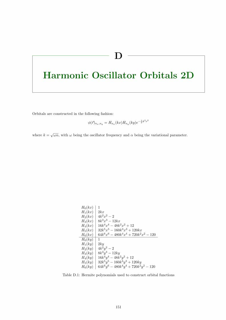
D
Harmonic Oscillator Orbitals 2D
Orbitals are constructed in the following fashion:
φ(~r)nx,ny= Hnx
(kx)Hny(ky)e−
12k
2r2
where k =√ωα, with ω being the oscillator frequency and α being the variational parameter.
H0(kx) 1H1(kx) 2kxH2(kx) 4k2x2 − 2H3(kx) 8k3x3 − 12kxH4(kx) 16k4x4 − 48k2x2 + 12H5(kx) 32k5x5 − 160k3x3 + 120kxH6(kx) 64k6x6 − 480k4x4 + 720k2x2 − 120H0(ky) 1H1(ky) 2kyH2(ky) 4k2y2 − 2H3(ky) 8k3y3 − 12kyH4(ky) 16k4y4 − 48k2y2 + 12H5(ky) 32k5y5 − 160k3y3 + 120kyH6(ky) 64k6y6 − 480k4y4 + 720k2y2 − 120
Table D.1: Hermite polynomials used to construct orbital functions
151
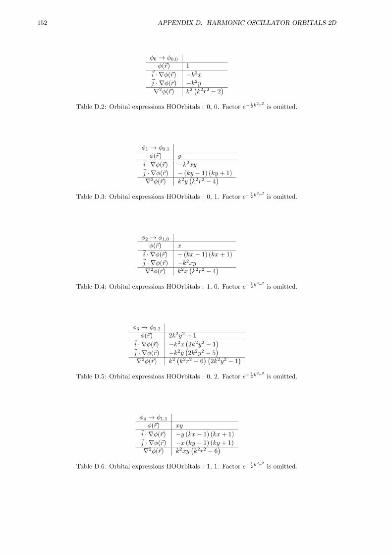
152 APPENDIX D. HARMONIC OSCILLATOR ORBITALS 2D
φ0 → φ0,0
φ(~r) 1~i · ∇φ(~r) −k2x~j · ∇φ(~r) −k2y
∇2φ(~r) k2(k2r2 − 2
)Table D.2: Orbital expressions HOOrbitals : 0, 0. Factor e−
12k
2r2 is omitted.
φ1 → φ0,1
φ(~r) y~i · ∇φ(~r) −k2xy~j · ∇φ(~r) − (ky − 1) (ky + 1)
∇2φ(~r) k2y(k2r2 − 4
)Table D.3: Orbital expressions HOOrbitals : 0, 1. Factor e−
12k
2r2 is omitted.
φ2 → φ1,0
φ(~r) x~i · ∇φ(~r) − (kx− 1) (kx+ 1)~j · ∇φ(~r) −k2xy
∇2φ(~r) k2x(k2r2 − 4
)Table D.4: Orbital expressions HOOrbitals : 1, 0. Factor e−
12k
2r2 is omitted.
φ3 → φ0,2
φ(~r) 2k2y2 − 1~i · ∇φ(~r) −k2x
(2k2y2 − 1
)~j · ∇φ(~r) −k2y
(2k2y2 − 5
)∇2φ(~r) k2
(k2r2 − 6
) (2k2y2 − 1
)Table D.5: Orbital expressions HOOrbitals : 0, 2. Factor e−
12k
2r2 is omitted.
φ4 → φ1,1
φ(~r) xy~i · ∇φ(~r) −y (kx− 1) (kx+ 1)~j · ∇φ(~r) −x (ky − 1) (ky + 1)
∇2φ(~r) k2xy(k2r2 − 6
)Table D.6: Orbital expressions HOOrbitals : 1, 1. Factor e−
12k
2r2 is omitted.
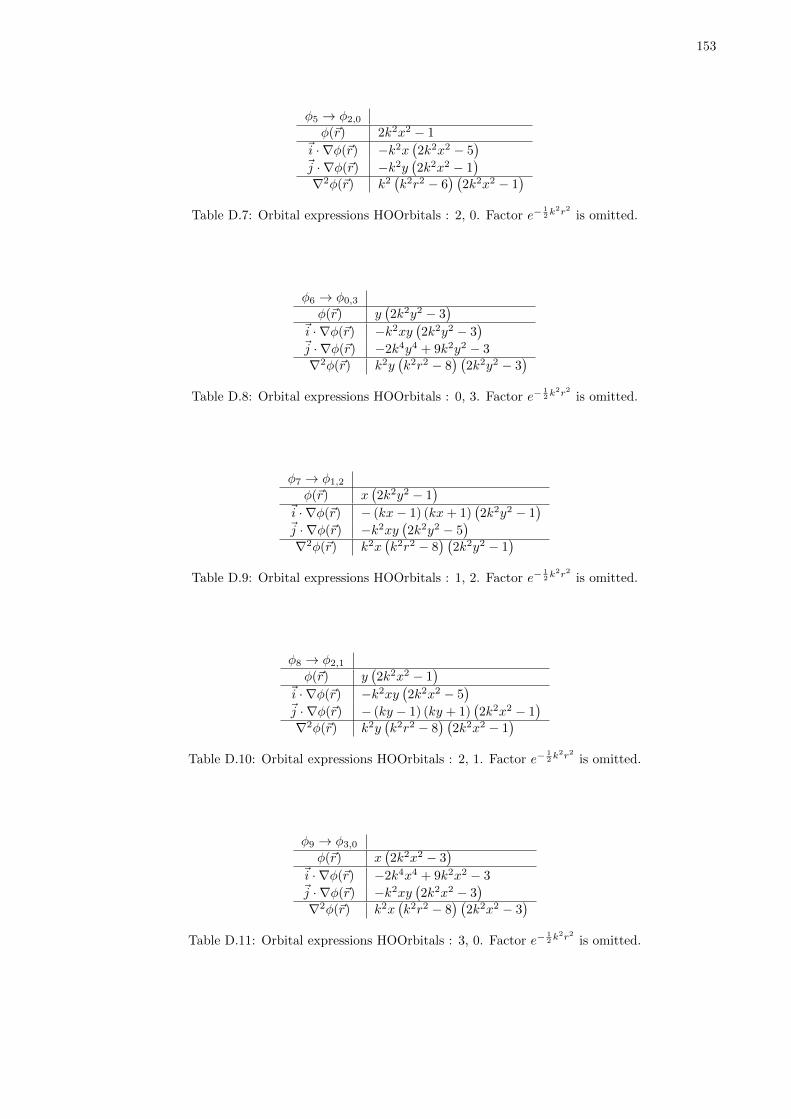
153
φ5 → φ2,0
φ(~r) 2k2x2 − 1~i · ∇φ(~r) −k2x
(2k2x2 − 5
)~j · ∇φ(~r) −k2y
(2k2x2 − 1
)∇2φ(~r) k2
(k2r2 − 6
) (2k2x2 − 1
)Table D.7: Orbital expressions HOOrbitals : 2, 0. Factor e−
12k
2r2 is omitted.
φ6 → φ0,3
φ(~r) y(2k2y2 − 3
)~i · ∇φ(~r) −k2xy
(2k2y2 − 3
)~j · ∇φ(~r) −2k4y4 + 9k2y2 − 3
∇2φ(~r) k2y(k2r2 − 8
) (2k2y2 − 3
)Table D.8: Orbital expressions HOOrbitals : 0, 3. Factor e−
12k
2r2 is omitted.
φ7 → φ1,2
φ(~r) x(2k2y2 − 1
)~i · ∇φ(~r) − (kx− 1) (kx+ 1)
(2k2y2 − 1
)~j · ∇φ(~r) −k2xy
(2k2y2 − 5
)∇2φ(~r) k2x
(k2r2 − 8
) (2k2y2 − 1
)Table D.9: Orbital expressions HOOrbitals : 1, 2. Factor e−
12k
2r2 is omitted.
φ8 → φ2,1
φ(~r) y(2k2x2 − 1
)~i · ∇φ(~r) −k2xy
(2k2x2 − 5
)~j · ∇φ(~r) − (ky − 1) (ky + 1)
(2k2x2 − 1
)∇2φ(~r) k2y
(k2r2 − 8
) (2k2x2 − 1
)Table D.10: Orbital expressions HOOrbitals : 2, 1. Factor e−
12k
2r2 is omitted.
φ9 → φ3,0
φ(~r) x(2k2x2 − 3
)~i · ∇φ(~r) −2k4x4 + 9k2x2 − 3~j · ∇φ(~r) −k2xy
(2k2x2 − 3
)∇2φ(~r) k2x
(k2r2 − 8
) (2k2x2 − 3
)Table D.11: Orbital expressions HOOrbitals : 3, 0. Factor e−
12k
2r2 is omitted.
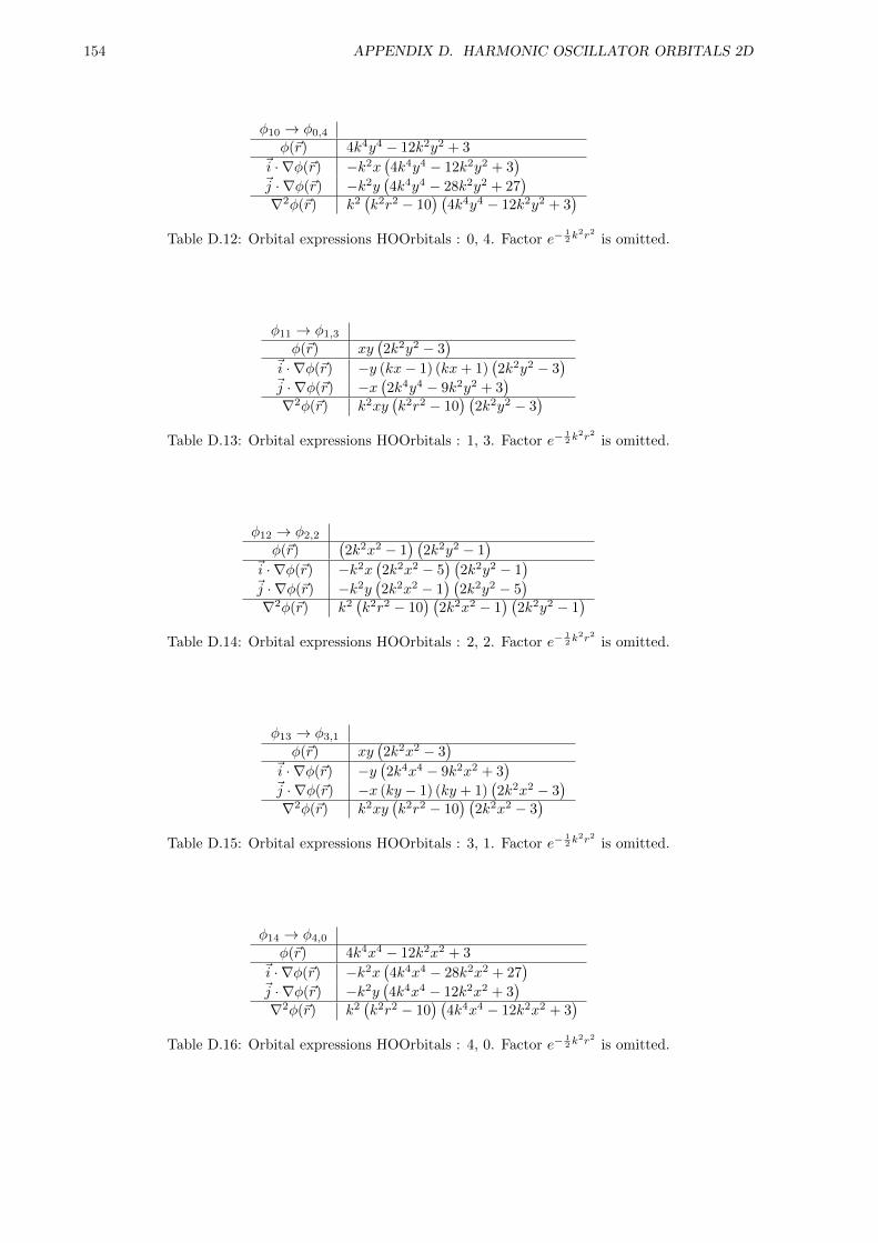
154 APPENDIX D. HARMONIC OSCILLATOR ORBITALS 2D
φ10 → φ0,4
φ(~r) 4k4y4 − 12k2y2 + 3~i · ∇φ(~r) −k2x
(4k4y4 − 12k2y2 + 3
)~j · ∇φ(~r) −k2y
(4k4y4 − 28k2y2 + 27
)∇2φ(~r) k2
(k2r2 − 10
) (4k4y4 − 12k2y2 + 3
)Table D.12: Orbital expressions HOOrbitals : 0, 4. Factor e−
12k
2r2 is omitted.
φ11 → φ1,3
φ(~r) xy(2k2y2 − 3
)~i · ∇φ(~r) −y (kx− 1) (kx+ 1)
(2k2y2 − 3
)~j · ∇φ(~r) −x
(2k4y4 − 9k2y2 + 3
)∇2φ(~r) k2xy
(k2r2 − 10
) (2k2y2 − 3
)Table D.13: Orbital expressions HOOrbitals : 1, 3. Factor e−
12k
2r2 is omitted.
φ12 → φ2,2
φ(~r)(2k2x2 − 1
) (2k2y2 − 1
)~i · ∇φ(~r) −k2x
(2k2x2 − 5
) (2k2y2 − 1
)~j · ∇φ(~r) −k2y
(2k2x2 − 1
) (2k2y2 − 5
)∇2φ(~r) k2
(k2r2 − 10
) (2k2x2 − 1
) (2k2y2 − 1
)Table D.14: Orbital expressions HOOrbitals : 2, 2. Factor e−
12k
2r2 is omitted.
φ13 → φ3,1
φ(~r) xy(2k2x2 − 3
)~i · ∇φ(~r) −y
(2k4x4 − 9k2x2 + 3
)~j · ∇φ(~r) −x (ky − 1) (ky + 1)
(2k2x2 − 3
)∇2φ(~r) k2xy
(k2r2 − 10
) (2k2x2 − 3
)Table D.15: Orbital expressions HOOrbitals : 3, 1. Factor e−
12k
2r2 is omitted.
φ14 → φ4,0
φ(~r) 4k4x4 − 12k2x2 + 3~i · ∇φ(~r) −k2x
(4k4x4 − 28k2x2 + 27
)~j · ∇φ(~r) −k2y
(4k4x4 − 12k2x2 + 3
)∇2φ(~r) k2
(k2r2 − 10
) (4k4x4 − 12k2x2 + 3
)Table D.16: Orbital expressions HOOrbitals : 4, 0. Factor e−
12k
2r2 is omitted.
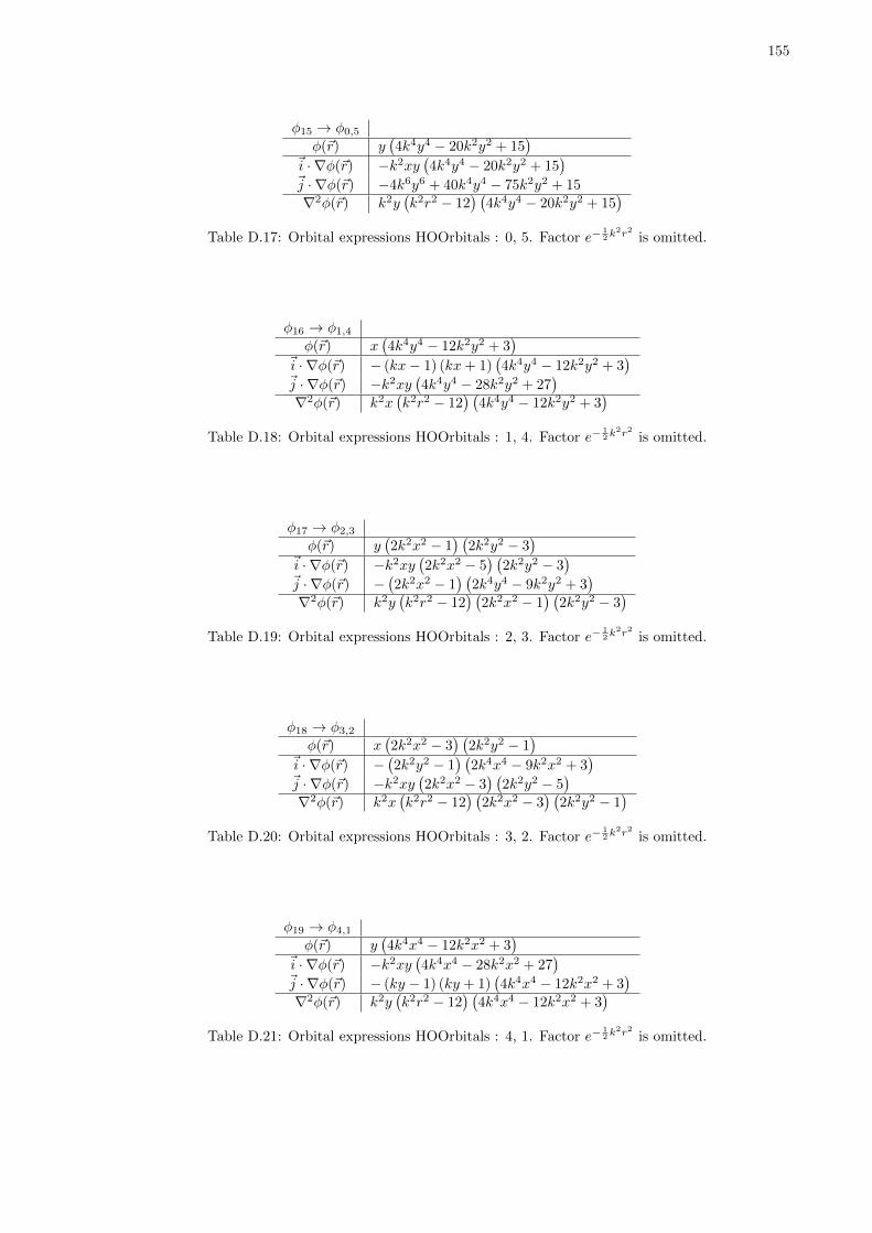
155
φ15 → φ0,5
φ(~r) y(4k4y4 − 20k2y2 + 15
)~i · ∇φ(~r) −k2xy
(4k4y4 − 20k2y2 + 15
)~j · ∇φ(~r) −4k6y6 + 40k4y4 − 75k2y2 + 15
∇2φ(~r) k2y(k2r2 − 12
) (4k4y4 − 20k2y2 + 15
)Table D.17: Orbital expressions HOOrbitals : 0, 5. Factor e−
12k
2r2 is omitted.
φ16 → φ1,4
φ(~r) x(4k4y4 − 12k2y2 + 3
)~i · ∇φ(~r) − (kx− 1) (kx+ 1)
(4k4y4 − 12k2y2 + 3
)~j · ∇φ(~r) −k2xy
(4k4y4 − 28k2y2 + 27
)∇2φ(~r) k2x
(k2r2 − 12
) (4k4y4 − 12k2y2 + 3
)Table D.18: Orbital expressions HOOrbitals : 1, 4. Factor e−
12k
2r2 is omitted.
φ17 → φ2,3
φ(~r) y(2k2x2 − 1
) (2k2y2 − 3
)~i · ∇φ(~r) −k2xy
(2k2x2 − 5
) (2k2y2 − 3
)~j · ∇φ(~r) −
(2k2x2 − 1
) (2k4y4 − 9k2y2 + 3
)∇2φ(~r) k2y
(k2r2 − 12
) (2k2x2 − 1
) (2k2y2 − 3
)Table D.19: Orbital expressions HOOrbitals : 2, 3. Factor e−
12k
2r2 is omitted.
φ18 → φ3,2
φ(~r) x(2k2x2 − 3
) (2k2y2 − 1
)~i · ∇φ(~r) −
(2k2y2 − 1
) (2k4x4 − 9k2x2 + 3
)~j · ∇φ(~r) −k2xy
(2k2x2 − 3
) (2k2y2 − 5
)∇2φ(~r) k2x
(k2r2 − 12
) (2k2x2 − 3
) (2k2y2 − 1
)Table D.20: Orbital expressions HOOrbitals : 3, 2. Factor e−
12k
2r2 is omitted.
φ19 → φ4,1
φ(~r) y(4k4x4 − 12k2x2 + 3
)~i · ∇φ(~r) −k2xy
(4k4x4 − 28k2x2 + 27
)~j · ∇φ(~r) − (ky − 1) (ky + 1)
(4k4x4 − 12k2x2 + 3
)∇2φ(~r) k2y
(k2r2 − 12
) (4k4x4 − 12k2x2 + 3
)Table D.21: Orbital expressions HOOrbitals : 4, 1. Factor e−
12k
2r2 is omitted.
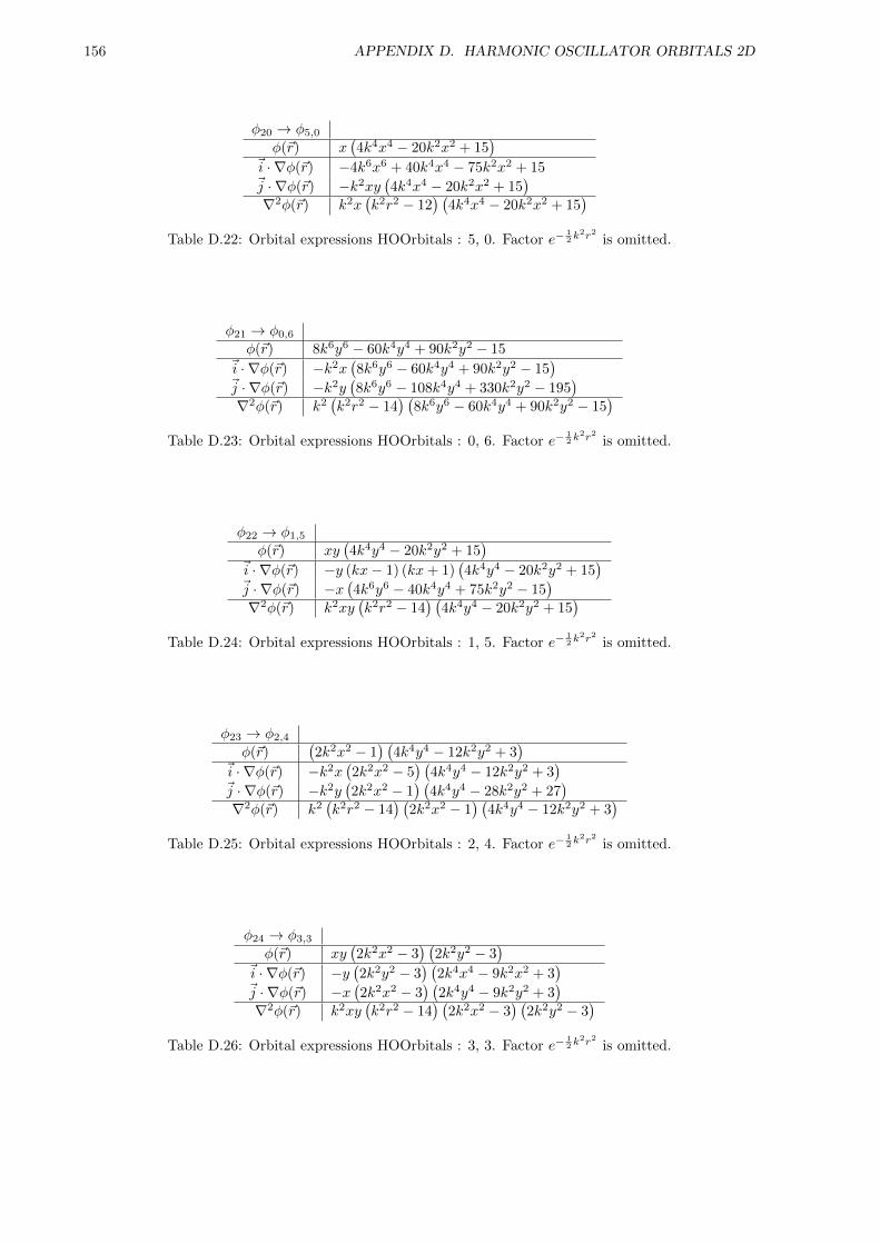
156 APPENDIX D. HARMONIC OSCILLATOR ORBITALS 2D
φ20 → φ5,0
φ(~r) x(4k4x4 − 20k2x2 + 15
)~i · ∇φ(~r) −4k6x6 + 40k4x4 − 75k2x2 + 15~j · ∇φ(~r) −k2xy
(4k4x4 − 20k2x2 + 15
)∇2φ(~r) k2x
(k2r2 − 12
) (4k4x4 − 20k2x2 + 15
)Table D.22: Orbital expressions HOOrbitals : 5, 0. Factor e−
12k
2r2 is omitted.
φ21 → φ0,6
φ(~r) 8k6y6 − 60k4y4 + 90k2y2 − 15~i · ∇φ(~r) −k2x
(8k6y6 − 60k4y4 + 90k2y2 − 15
)~j · ∇φ(~r) −k2y
(8k6y6 − 108k4y4 + 330k2y2 − 195
)∇2φ(~r) k2
(k2r2 − 14
) (8k6y6 − 60k4y4 + 90k2y2 − 15
)Table D.23: Orbital expressions HOOrbitals : 0, 6. Factor e−
12k
2r2 is omitted.
φ22 → φ1,5
φ(~r) xy(4k4y4 − 20k2y2 + 15
)~i · ∇φ(~r) −y (kx− 1) (kx+ 1)
(4k4y4 − 20k2y2 + 15
)~j · ∇φ(~r) −x
(4k6y6 − 40k4y4 + 75k2y2 − 15
)∇2φ(~r) k2xy
(k2r2 − 14
) (4k4y4 − 20k2y2 + 15
)Table D.24: Orbital expressions HOOrbitals : 1, 5. Factor e−
12k
2r2 is omitted.
φ23 → φ2,4
φ(~r)(2k2x2 − 1
) (4k4y4 − 12k2y2 + 3
)~i · ∇φ(~r) −k2x
(2k2x2 − 5
) (4k4y4 − 12k2y2 + 3
)~j · ∇φ(~r) −k2y
(2k2x2 − 1
) (4k4y4 − 28k2y2 + 27
)∇2φ(~r) k2
(k2r2 − 14
) (2k2x2 − 1
) (4k4y4 − 12k2y2 + 3
)Table D.25: Orbital expressions HOOrbitals : 2, 4. Factor e−
12k
2r2 is omitted.
φ24 → φ3,3
φ(~r) xy(2k2x2 − 3
) (2k2y2 − 3
)~i · ∇φ(~r) −y
(2k2y2 − 3
) (2k4x4 − 9k2x2 + 3
)~j · ∇φ(~r) −x
(2k2x2 − 3
) (2k4y4 − 9k2y2 + 3
)∇2φ(~r) k2xy
(k2r2 − 14
) (2k2x2 − 3
) (2k2y2 − 3
)Table D.26: Orbital expressions HOOrbitals : 3, 3. Factor e−
12k
2r2 is omitted.
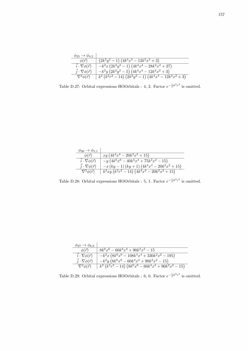
157
φ25 → φ4,2
φ(~r)(2k2y2 − 1
) (4k4x4 − 12k2x2 + 3
)~i · ∇φ(~r) −k2x
(2k2y2 − 1
) (4k4x4 − 28k2x2 + 27
)~j · ∇φ(~r) −k2y
(2k2y2 − 5
) (4k4x4 − 12k2x2 + 3
)∇2φ(~r) k2
(k2r2 − 14
) (2k2y2 − 1
) (4k4x4 − 12k2x2 + 3
)Table D.27: Orbital expressions HOOrbitals : 4, 2. Factor e−
12k
2r2 is omitted.
φ26 → φ5,1
φ(~r) xy(4k4x4 − 20k2x2 + 15
)~i · ∇φ(~r) −y
(4k6x6 − 40k4x4 + 75k2x2 − 15
)~j · ∇φ(~r) −x (ky − 1) (ky + 1)
(4k4x4 − 20k2x2 + 15
)∇2φ(~r) k2xy
(k2r2 − 14
) (4k4x4 − 20k2x2 + 15
)Table D.28: Orbital expressions HOOrbitals : 5, 1. Factor e−
12k
2r2 is omitted.
φ27 → φ6,0
φ(~r) 8k6x6 − 60k4x4 + 90k2x2 − 15~i · ∇φ(~r) −k2x
(8k6x6 − 108k4x4 + 330k2x2 − 195
)~j · ∇φ(~r) −k2y
(8k6x6 − 60k4x4 + 90k2x2 − 15
)∇2φ(~r) k2
(k2r2 − 14
) (8k6x6 − 60k4x4 + 90k2x2 − 15
)Table D.29: Orbital expressions HOOrbitals : 6, 0. Factor e−
12k
2r2 is omitted.

158

E
Harmonic Oscillator Orbitals 3D
Orbitals are constructed in the following fashion:
φ(~r)nx,ny,nz= Hnx
(kx)Hny(ky)Hnz
(kz)e−12k
2r2
where k =√ωα, with ω being the oscillator frequency and α being the variational parameter.
H0(kx) 1H1(kx) 2kxH2(kx) 4k2x2 − 2H3(kx) 8k3x3 − 12kxH0(ky) 1H1(ky) 2kyH2(ky) 4k2y2 − 2H3(ky) 8k3y3 − 12kyH0(kz) 1H1(kz) 2kzH2(kz) 4k2z2 − 2H3(kz) 8k3z3 − 12kz
Table E.1: Hermite polynomials used to construct orbital functions
159
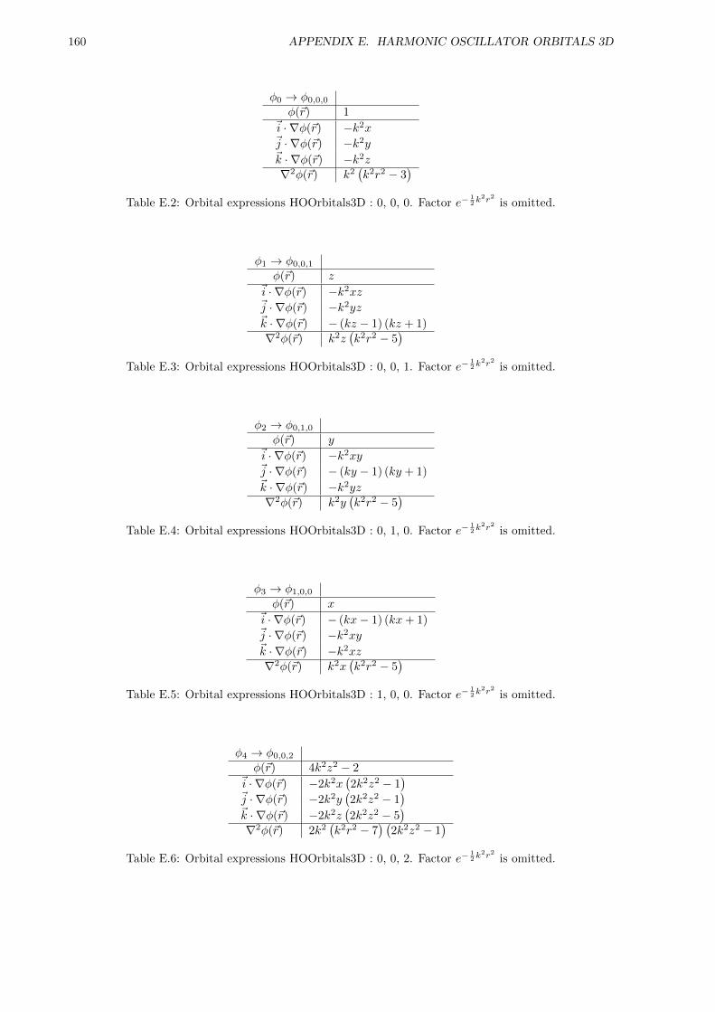
160 APPENDIX E. HARMONIC OSCILLATOR ORBITALS 3D
φ0 → φ0,0,0
φ(~r) 1~i · ∇φ(~r) −k2x~j · ∇φ(~r) −k2y~k · ∇φ(~r) −k2z
∇2φ(~r) k2(k2r2 − 3
)Table E.2: Orbital expressions HOOrbitals3D : 0, 0, 0. Factor e−
12k
2r2 is omitted.
φ1 → φ0,0,1
φ(~r) z~i · ∇φ(~r) −k2xz~j · ∇φ(~r) −k2yz~k · ∇φ(~r) − (kz − 1) (kz + 1)
∇2φ(~r) k2z(k2r2 − 5
)Table E.3: Orbital expressions HOOrbitals3D : 0, 0, 1. Factor e−
12k
2r2 is omitted.
φ2 → φ0,1,0
φ(~r) y~i · ∇φ(~r) −k2xy~j · ∇φ(~r) − (ky − 1) (ky + 1)~k · ∇φ(~r) −k2yz
∇2φ(~r) k2y(k2r2 − 5
)Table E.4: Orbital expressions HOOrbitals3D : 0, 1, 0. Factor e−
12k
2r2 is omitted.
φ3 → φ1,0,0
φ(~r) x~i · ∇φ(~r) − (kx− 1) (kx+ 1)~j · ∇φ(~r) −k2xy~k · ∇φ(~r) −k2xz
∇2φ(~r) k2x(k2r2 − 5
)Table E.5: Orbital expressions HOOrbitals3D : 1, 0, 0. Factor e−
12k
2r2 is omitted.
φ4 → φ0,0,2
φ(~r) 4k2z2 − 2~i · ∇φ(~r) −2k2x
(2k2z2 − 1
)~j · ∇φ(~r) −2k2y
(2k2z2 − 1
)~k · ∇φ(~r) −2k2z
(2k2z2 − 5
)∇2φ(~r) 2k2
(k2r2 − 7
) (2k2z2 − 1
)Table E.6: Orbital expressions HOOrbitals3D : 0, 0, 2. Factor e−
12k
2r2 is omitted.
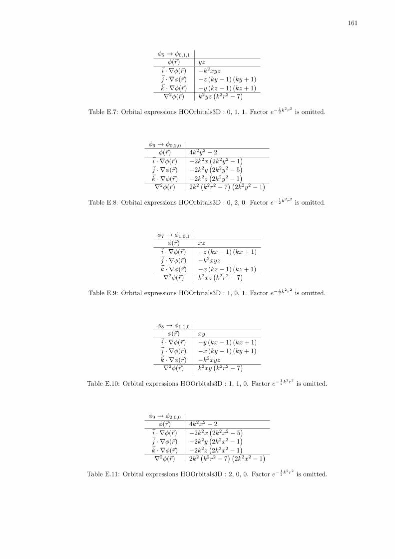
161
φ5 → φ0,1,1
φ(~r) yz~i · ∇φ(~r) −k2xyz~j · ∇φ(~r) −z (ky − 1) (ky + 1)~k · ∇φ(~r) −y (kz − 1) (kz + 1)
∇2φ(~r) k2yz(k2r2 − 7
)Table E.7: Orbital expressions HOOrbitals3D : 0, 1, 1. Factor e−
12k
2r2 is omitted.
φ6 → φ0,2,0
φ(~r) 4k2y2 − 2~i · ∇φ(~r) −2k2x
(2k2y2 − 1
)~j · ∇φ(~r) −2k2y
(2k2y2 − 5
)~k · ∇φ(~r) −2k2z
(2k2y2 − 1
)∇2φ(~r) 2k2
(k2r2 − 7
) (2k2y2 − 1
)Table E.8: Orbital expressions HOOrbitals3D : 0, 2, 0. Factor e−
12k
2r2 is omitted.
φ7 → φ1,0,1
φ(~r) xz~i · ∇φ(~r) −z (kx− 1) (kx+ 1)~j · ∇φ(~r) −k2xyz~k · ∇φ(~r) −x (kz − 1) (kz + 1)
∇2φ(~r) k2xz(k2r2 − 7
)Table E.9: Orbital expressions HOOrbitals3D : 1, 0, 1. Factor e−
12k
2r2 is omitted.
φ8 → φ1,1,0
φ(~r) xy~i · ∇φ(~r) −y (kx− 1) (kx+ 1)~j · ∇φ(~r) −x (ky − 1) (ky + 1)~k · ∇φ(~r) −k2xyz
∇2φ(~r) k2xy(k2r2 − 7
)Table E.10: Orbital expressions HOOrbitals3D : 1, 1, 0. Factor e−
12k
2r2 is omitted.
φ9 → φ2,0,0
φ(~r) 4k2x2 − 2~i · ∇φ(~r) −2k2x
(2k2x2 − 5
)~j · ∇φ(~r) −2k2y
(2k2x2 − 1
)~k · ∇φ(~r) −2k2z
(2k2x2 − 1
)∇2φ(~r) 2k2
(k2r2 − 7
) (2k2x2 − 1
)Table E.11: Orbital expressions HOOrbitals3D : 2, 0, 0. Factor e−
12k
2r2 is omitted.
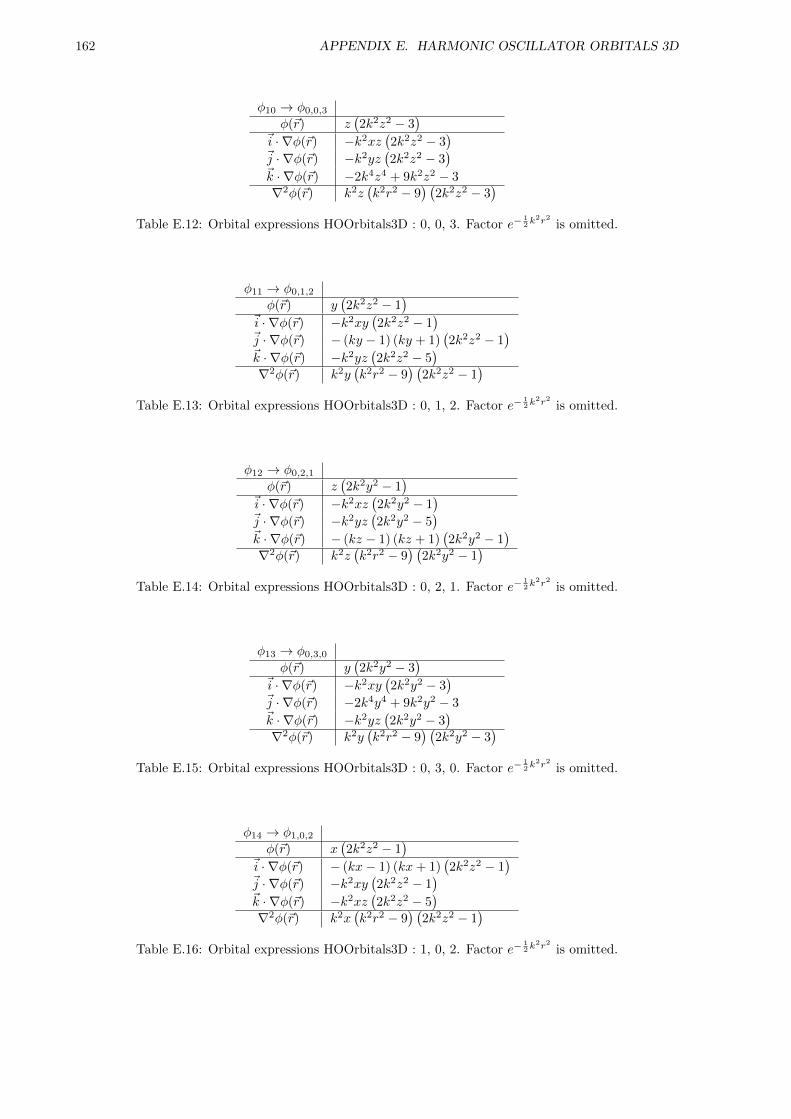
162 APPENDIX E. HARMONIC OSCILLATOR ORBITALS 3D
φ10 → φ0,0,3
φ(~r) z(2k2z2 − 3
)~i · ∇φ(~r) −k2xz
(2k2z2 − 3
)~j · ∇φ(~r) −k2yz
(2k2z2 − 3
)~k · ∇φ(~r) −2k4z4 + 9k2z2 − 3
∇2φ(~r) k2z(k2r2 − 9
) (2k2z2 − 3
)Table E.12: Orbital expressions HOOrbitals3D : 0, 0, 3. Factor e−
12k
2r2 is omitted.
φ11 → φ0,1,2
φ(~r) y(2k2z2 − 1
)~i · ∇φ(~r) −k2xy
(2k2z2 − 1
)~j · ∇φ(~r) − (ky − 1) (ky + 1)
(2k2z2 − 1
)~k · ∇φ(~r) −k2yz
(2k2z2 − 5
)∇2φ(~r) k2y
(k2r2 − 9
) (2k2z2 − 1
)Table E.13: Orbital expressions HOOrbitals3D : 0, 1, 2. Factor e−
12k
2r2 is omitted.
φ12 → φ0,2,1
φ(~r) z(2k2y2 − 1
)~i · ∇φ(~r) −k2xz
(2k2y2 − 1
)~j · ∇φ(~r) −k2yz
(2k2y2 − 5
)~k · ∇φ(~r) − (kz − 1) (kz + 1)
(2k2y2 − 1
)∇2φ(~r) k2z
(k2r2 − 9
) (2k2y2 − 1
)Table E.14: Orbital expressions HOOrbitals3D : 0, 2, 1. Factor e−
12k
2r2 is omitted.
φ13 → φ0,3,0
φ(~r) y(2k2y2 − 3
)~i · ∇φ(~r) −k2xy
(2k2y2 − 3
)~j · ∇φ(~r) −2k4y4 + 9k2y2 − 3~k · ∇φ(~r) −k2yz
(2k2y2 − 3
)∇2φ(~r) k2y
(k2r2 − 9
) (2k2y2 − 3
)Table E.15: Orbital expressions HOOrbitals3D : 0, 3, 0. Factor e−
12k
2r2 is omitted.
φ14 → φ1,0,2
φ(~r) x(2k2z2 − 1
)~i · ∇φ(~r) − (kx− 1) (kx+ 1)
(2k2z2 − 1
)~j · ∇φ(~r) −k2xy
(2k2z2 − 1
)~k · ∇φ(~r) −k2xz
(2k2z2 − 5
)∇2φ(~r) k2x
(k2r2 − 9
) (2k2z2 − 1
)Table E.16: Orbital expressions HOOrbitals3D : 1, 0, 2. Factor e−
12k
2r2 is omitted.
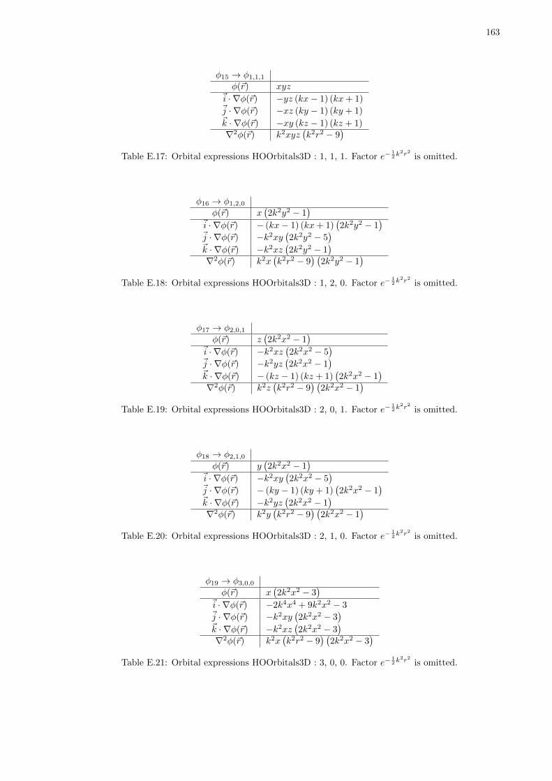
163
φ15 → φ1,1,1
φ(~r) xyz~i · ∇φ(~r) −yz (kx− 1) (kx+ 1)~j · ∇φ(~r) −xz (ky − 1) (ky + 1)~k · ∇φ(~r) −xy (kz − 1) (kz + 1)
∇2φ(~r) k2xyz(k2r2 − 9
)Table E.17: Orbital expressions HOOrbitals3D : 1, 1, 1. Factor e−
12k
2r2 is omitted.
φ16 → φ1,2,0
φ(~r) x(2k2y2 − 1
)~i · ∇φ(~r) − (kx− 1) (kx+ 1)
(2k2y2 − 1
)~j · ∇φ(~r) −k2xy
(2k2y2 − 5
)~k · ∇φ(~r) −k2xz
(2k2y2 − 1
)∇2φ(~r) k2x
(k2r2 − 9
) (2k2y2 − 1
)Table E.18: Orbital expressions HOOrbitals3D : 1, 2, 0. Factor e−
12k
2r2 is omitted.
φ17 → φ2,0,1
φ(~r) z(2k2x2 − 1
)~i · ∇φ(~r) −k2xz
(2k2x2 − 5
)~j · ∇φ(~r) −k2yz
(2k2x2 − 1
)~k · ∇φ(~r) − (kz − 1) (kz + 1)
(2k2x2 − 1
)∇2φ(~r) k2z
(k2r2 − 9
) (2k2x2 − 1
)Table E.19: Orbital expressions HOOrbitals3D : 2, 0, 1. Factor e−
12k
2r2 is omitted.
φ18 → φ2,1,0
φ(~r) y(2k2x2 − 1
)~i · ∇φ(~r) −k2xy
(2k2x2 − 5
)~j · ∇φ(~r) − (ky − 1) (ky + 1)
(2k2x2 − 1
)~k · ∇φ(~r) −k2yz
(2k2x2 − 1
)∇2φ(~r) k2y
(k2r2 − 9
) (2k2x2 − 1
)Table E.20: Orbital expressions HOOrbitals3D : 2, 1, 0. Factor e−
12k
2r2 is omitted.
φ19 → φ3,0,0
φ(~r) x(2k2x2 − 3
)~i · ∇φ(~r) −2k4x4 + 9k2x2 − 3~j · ∇φ(~r) −k2xy
(2k2x2 − 3
)~k · ∇φ(~r) −k2xz
(2k2x2 − 3
)∇2φ(~r) k2x
(k2r2 − 9
) (2k2x2 − 3
)Table E.21: Orbital expressions HOOrbitals3D : 3, 0, 0. Factor e−
12k
2r2 is omitted.

164
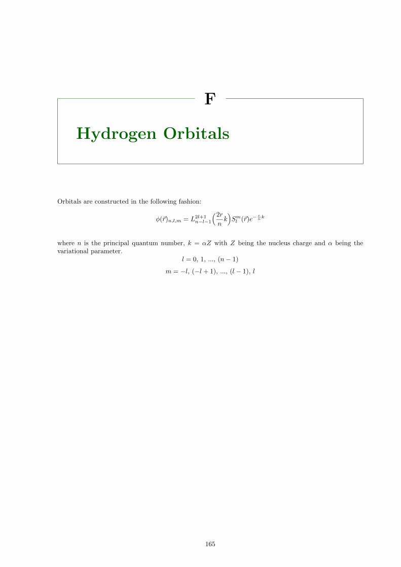
F
Hydrogen Orbitals
Orbitals are constructed in the following fashion:
φ(~r)n,l,m = L2l+1n−l−1
(2r
nk)Sml (~r)e−
rnk
where n is the principal quantum number, k = αZ with Z being the nucleus charge and α being thevariational parameter.
l = 0, 1, ..., (n− 1)
m = −l, (−l + 1), ..., (l − 1), l
165
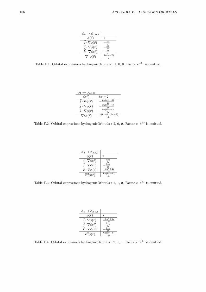
166 APPENDIX F. HYDROGEN ORBITALS
φ0 → φ1,0,0
φ(~r) 1~i · ∇φ(~r) −kxr~j · ∇φ(~r) −kyr~k · ∇φ(~r) −kzr∇2φ(~r) k(kr−2)
r
Table F.1: Orbital expressions hydrogenicOrbitals : 1, 0, 0. Factor e−kr is omitted.
φ1 → φ2,0,0
φ(~r) kr − 2~i · ∇φ(~r) −kx(kr−4)
2r~j · ∇φ(~r) −ky(kr−4)
2r~k · ∇φ(~r) −kz(kr−4)
2r
∇2φ(~r) k(kr−8)(kr−2)4r
Table F.2: Orbital expressions hydrogenicOrbitals : 2, 0, 0. Factor e−12kr is omitted.
φ2 → φ2,1,0
φ(~r) z~i · ∇φ(~r) −kxz2r~j · ∇φ(~r) −kyz2r~k · ∇φ(~r) −kz2+2r
2r
∇2φ(~r) kz(kr−8)4r
Table F.3: Orbital expressions hydrogenicOrbitals : 2, 1, 0. Factor e−12kr is omitted.
φ3 → φ2,1,1
φ(~r) x~i · ∇φ(~r) −kx2+2r
2r~j · ∇φ(~r) −kxy2r~k · ∇φ(~r) −kxz2r
∇2φ(~r) kx(kr−8)4r
Table F.4: Orbital expressions hydrogenicOrbitals : 2, 1, 1. Factor e−12kr is omitted.
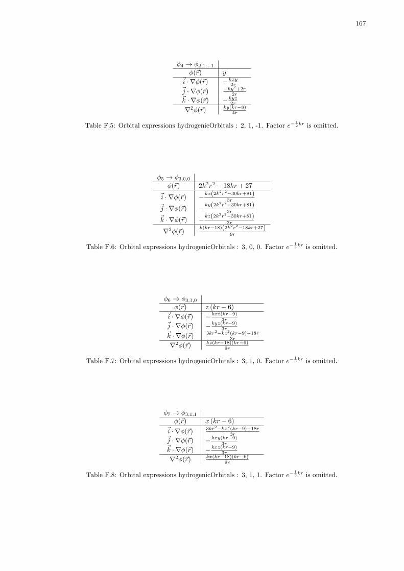
167
φ4 → φ2,1,−1
φ(~r) y~i · ∇φ(~r) −kxy2r~j · ∇φ(~r) −ky2+2r
2r~k · ∇φ(~r) −kyz2r
∇2φ(~r) ky(kr−8)4r
Table F.5: Orbital expressions hydrogenicOrbitals : 2, 1, -1. Factor e−12kr is omitted.
φ5 → φ3,0,0
φ(~r) 2k2r2 − 18kr + 27
~i · ∇φ(~r) −kx(2k2r2−30kr+81)3r
~j · ∇φ(~r) −ky(2k2r2−30kr+81)3r
~k · ∇φ(~r) −kz(2k2r2−30kr+81)3r
∇2φ(~r)k(kr−18)(2k2r2−18kr+27)
9r
Table F.6: Orbital expressions hydrogenicOrbitals : 3, 0, 0. Factor e−13kr is omitted.
φ6 → φ3,1,0
φ(~r) z (kr − 6)~i · ∇φ(~r) −kxz(kr−9)
3r~j · ∇φ(~r) −kyz(kr−9)
3r~k · ∇φ(~r) 3kr2−kz2(kr−9)−18r
3r
∇2φ(~r) kz(kr−18)(kr−6)9r
Table F.7: Orbital expressions hydrogenicOrbitals : 3, 1, 0. Factor e−13kr is omitted.
φ7 → φ3,1,1
φ(~r) x (kr − 6)
~i · ∇φ(~r) 3kr2−kx2(kr−9)−18r3r
~j · ∇φ(~r) −kxy(kr−9)3r
~k · ∇φ(~r) −kxz(kr−9)3r
∇2φ(~r) kx(kr−18)(kr−6)9r
Table F.8: Orbital expressions hydrogenicOrbitals : 3, 1, 1. Factor e−13kr is omitted.
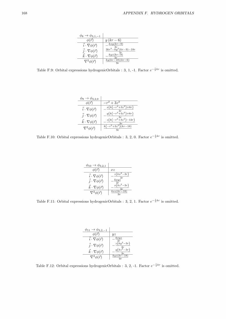
168 APPENDIX F. HYDROGEN ORBITALS
φ8 → φ3,1,−1
φ(~r) y (kr − 6)~i · ∇φ(~r) −kxy(kr−9)
3r
~j · ∇φ(~r) 3kr2−ky2(kr−9)−18r3r
~k · ∇φ(~r) −kyz(kr−9)3r
∇2φ(~r) ky(kr−18)(kr−6)9r
Table F.9: Orbital expressions hydrogenicOrbitals : 3, 1, -1. Factor e−13kr is omitted.
φ9 → φ3,2,0
φ(~r) −r2 + 3z2
~i · ∇φ(~r) −x(k(−r2+3z2)+6r)3r
~j · ∇φ(~r) −y(k(−r2+3z2)+6r)
3r
~k · ∇φ(~r) − z(k(−r2+3z2)−12r)
3r
∇2φ(~r)k(−r2+3z2)(kr−18)
9r
Table F.10: Orbital expressions hydrogenicOrbitals : 3, 2, 0. Factor e−13kr is omitted.
φ10 → φ3,2,1
φ(~r) xz
~i · ∇φ(~r) − z(kx2−3r)3r
~j · ∇φ(~r) −kxyz3r
~k · ∇φ(~r) −x(kz2−3r)3r
∇2φ(~r) kxz(kr−18)9r
Table F.11: Orbital expressions hydrogenicOrbitals : 3, 2, 1. Factor e−13kr is omitted.
φ11 → φ3,2,−1
φ(~r) yz~i · ∇φ(~r) −kxyz3r
~j · ∇φ(~r) − z(ky2−3r)3r
~k · ∇φ(~r) −y(kz2−3r)3r
∇2φ(~r) kyz(kr−18)9r
Table F.12: Orbital expressions hydrogenicOrbitals : 3, 2, -1. Factor e−13kr is omitted.
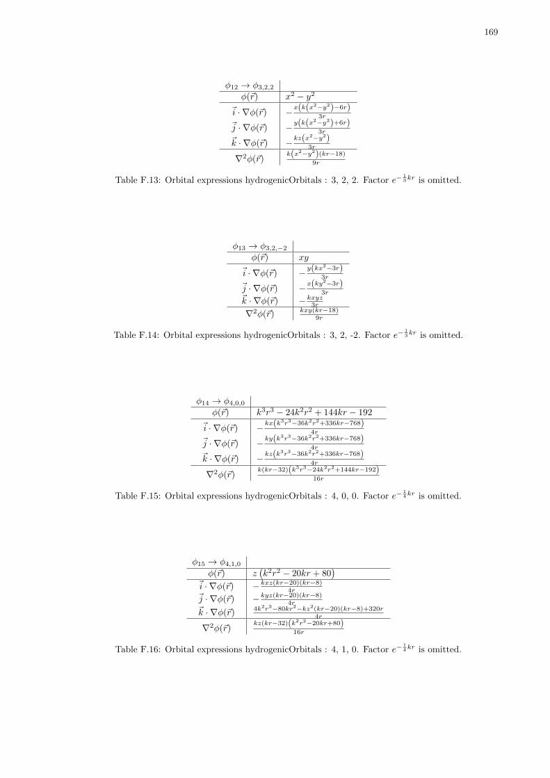
169
φ12 → φ3,2,2
φ(~r) x2 − y2
~i · ∇φ(~r) −x(k(x2−y2)−6r)
3r
~j · ∇φ(~r) −y(k(x2−y2)+6r)
3r
~k · ∇φ(~r) −kz(x2−y2)3r
∇2φ(~r)k(x2−y2)(kr−18)
9r
Table F.13: Orbital expressions hydrogenicOrbitals : 3, 2, 2. Factor e−13kr is omitted.
φ13 → φ3,2,−2
φ(~r) xy
~i · ∇φ(~r) −y(kx2−3r)3r
~j · ∇φ(~r) −x(ky2−3r)3r
~k · ∇φ(~r) −kxyz3r
∇2φ(~r) kxy(kr−18)9r
Table F.14: Orbital expressions hydrogenicOrbitals : 3, 2, -2. Factor e−13kr is omitted.
φ14 → φ4,0,0
φ(~r) k3r3 − 24k2r2 + 144kr − 192
~i · ∇φ(~r) −kx(k3r3−36k2r2+336kr−768)
4r
~j · ∇φ(~r) −ky(k3r3−36k2r2+336kr−768)
4r
~k · ∇φ(~r) −kz(k3r3−36k2r2+336kr−768)
4r
∇2φ(~r)k(kr−32)(k3r3−24k2r2+144kr−192)
16r
Table F.15: Orbital expressions hydrogenicOrbitals : 4, 0, 0. Factor e−14kr is omitted.
φ15 → φ4,1,0
φ(~r) z(k2r2 − 20kr + 80
)~i · ∇φ(~r) −kxz(kr−20)(kr−8)
4r~j · ∇φ(~r) −kyz(kr−20)(kr−8)
4r~k · ∇φ(~r) 4k2r3−80kr2−kz2(kr−20)(kr−8)+320r
4r
∇2φ(~r)kz(kr−32)(k2r2−20kr+80)
16r
Table F.16: Orbital expressions hydrogenicOrbitals : 4, 1, 0. Factor e−14kr is omitted.

170 APPENDIX F. HYDROGEN ORBITALS
φ16 → φ4,1,1
φ(~r) x(k2r2 − 20kr + 80
)~i · ∇φ(~r) 4k2r3−80kr2−kx2(kr−20)(kr−8)+320r
4r~j · ∇φ(~r) −kxy(kr−20)(kr−8)
4r~k · ∇φ(~r) −kxz(kr−20)(kr−8)
4r
∇2φ(~r)kx(kr−32)(k2r2−20kr+80)
16r
Table F.17: Orbital expressions hydrogenicOrbitals : 4, 1, 1. Factor e−14kr is omitted.
φ17 → φ4,1,−1
φ(~r) y(k2r2 − 20kr + 80
)~i · ∇φ(~r) −kxy(kr−20)(kr−8)
4r
~j · ∇φ(~r) 4k2r3−80kr2−ky2(kr−20)(kr−8)+320r4r
~k · ∇φ(~r) −kyz(kr−20)(kr−8)4r
∇2φ(~r)ky(kr−32)(k2r2−20kr+80)
16r
Table F.18: Orbital expressions hydrogenicOrbitals : 4, 1, -1. Factor e−14kr is omitted.
Bibliography
[1] S. Reimann, J. Høgberget, M. Hjorth-Jensen, and S. K. Bogner.In-medium similarity renormalization group approach studies ofquantum dots. In preparation, 2013.
[2] Christoffer Hirth. Studies of quantum dots: Ab initio coupled-cluster analysis using OpenCL and GPU programming. Master’sthesis, University of Oslo, 2012.
[3] Moskowitz Kalos. A new Look at Correlations in Atomic andMolecular Systems. Application of Fermion Monte Carlo Varia-tional Method. Int. J. Quant. Chem., XX:1107, 1981.
[4] S. Datta, S. A. Alexander, and R. L. Coldwell. Properties ofselected diatomics using variational Monte Carlo methods. J.Chem. Phys., 120:3642, 2004.
[5] Matthias Degroote. Faddeev random phase approximation ap-plied to molecules. Eur. Phys. J. ST, 218:1, 2013.
[6] Harry Partridge. Near Hartree–Fock quality GTO basis sets forthe first- and third-row atoms. J. Chem. Phys., 90:1043, 1989.
[7] A Badinski, P D Haynes, J R Trail, and R J Needs. Methodsfor calculating forces within quantum Monte Carlo simulations.J. Phys.: Condens. Matter, 22:074202, 2010.
[8] Veronica K. B. Olsen. Full Configuration Interaction Simulationof Quantum Dots. Master’s thesis, University of Oslo, 2012.
[9] Jørgen Høgberget. Git Repository: LibBorealis, 2013.http://www.github.com/jorgehog/QMC2.
[10] Murat Barisik and Ali Beskok. Equilibrium molecular dynam-ics studies on nanoscale-confined fluids. Microfluid Nanofluid,11(3):269, September 2011.
[11] Karl P. Travis and Keith E. Gubbins. Poiseuille flow of Lennard-Jones fluids in narrow slit pores. J. Chem. Phys, 112:1984, 2000.
[12] Charles J. Murray. The SUPERMEN. New York: Wiley, 1997.
[13] Hans Petter Langtangen. Python Scripting for ComputationalScience. Springer, 3rd edition, 2008.
171
172 BIBLIOGRAPHY
[14] Mark Lutz. Programming Python - powerful object-oriented pro-gramming. O’Reilly, 3rd edition, 2006.
[15] Hans Petter Langtangen. A primer on scientific programmingwith Python. Springer, Berlin; Heidelberg; New York, 2011.
[16] Gerard O’Regan. A Brief History of Computing, Second Edition.Springer, 2012.
[17] David Griffiths. Introduction to Quantum Mechanics. Pearson,2nd edition edition, 2005.
[18] I. Shavitt and R. J. Bartlett. Many-Body Methods in Chemistryand Physics. Cambridge University Press, Cambridge, 2009.
[19] Sigve B. Skattum. Time Evolution of Quantum Dots. Master’sthesis, University of Oslo, 2013.
[20] J. J. Mares et al. Periodic reactions and quantum diffusion.http://www.fzu.cz/ sestak/yyx/periodic%20reactions.pdf.
[21] B.L. Hammond, Jr. W. A. Lester, and P. J. Reynolds. MonteCarlo Methods in Ab Initio Quantum Chemistry. World Scien-tific Publishing Co., 1994.
[22] C. W Gardiner. Handbook of stochastic methods for physics,chemistry, and the natural sciences. Springer-Verlag, Berlin, 3rdedition, 2004.
[23] H. Risken and H. Haken. The Fokker-Planck Equation: Methodsof Solution and Applications Second Edition. Springer, 1989.
[24] W. T Coffey, Y. P Kalmykov, and J. T Waldron. The LangevinEquation: With Applications to Stochastic Problems in Physics,Chemistry, and Electrical Engineering. . World Scientific, Sin-gapore, 2004.
[25] C.P. Robert and G. Casella. Monte Carlo Statistical Methods.Springer Verlag, 2004.
[26] Morten Hjorth-Jensen. Computational Physics. 2010.
[27] J. J. Sakurai. Modern Quantum Mechanics. Addison-Wesley,New York, Revised ed edition, 1994.
[28] Lars Eivind Lervag. VMC Calculations of Two-dimensionalQuantum Dots. Master’s thesis, University of Oslo, 2010.
[29] Daniel Andres Nissenbaum. The stochastic gradient approxima-tion: an application to li nanoclusters. PhD thesis, NortheasternUniversity, 2008.
[30] Claudia Filippi and C. J. Umrigar. Multiconfiguration wavefunction for quantum Monte Carlo calculations of first-row di-atomic molecules. J. Chem. Phys, 105:213, July 1996.
[31] G.H. Golub and C.F. Van Loan. Matrix computations, volume 3.Johns Hopkins Univ Press, 1996.
[32] A. Harju, B. Barbiellini, S. Siljamaki, R. M. Nieminen,and G. Ortiz. Stochastic Gradient Approximation: AnEfficient Method to Optimize Many-Body Wave Functions.Phys. Rev. Lett., page 1173, August 1997.
BIBLIOGRAPHY 173
[33] Stefan Klein, Josien P. W. Pluim, Marius Staring, and Max A.Viergever. Adaptive Stochastic Gradient Descent Optimisationfor Image Registration. Int. J. Comput. Vision, page 227, 2009.
[34] Jon Magne Leinaas. Non-Relativistic Quantum Mechanics. lec-ture notes FYS4110.
[35] H. Flyvbjerg and H. G. Petersen. Error estimates on averagesof correlated data. J. Chem. Phys, 91:461, 1989.
[36] David C. Lay. Linear Algebra and its Applications. Pearson, 4edition, 2012.
[37] Jaime Fernandez Rico, Rafael Lopez, Ignacio Ema, andGuillermo Ramırez. Translation of real solid spherical harmon-ics. Int. J. Quant. Chem., 113:1544, 2013.
[38] T. Helgaker, P. Jørgensen, and J. Olsen. Molecular Electronic-Structure Theory. Wiley, Chichester, 2000.
[39] A. Kongkanand, K. Tvrdy, K. Takechi, M. Kuno, and P. V.Kamat. Quantum dot solar cells. Tuning photoresponse throughsize and shape control of CdSe-TiO2 architecture. J. Am. Chem.Soc., 130:4007, March 2008.
[40] G. Park, O.B. Shchekin, D.L. Huffaker, and D.G. Deppe. Low-threshold oxide-confined 1.3- micrometer quantum-dot laser.IEEE Photon. Technol. Lett., 12:230, 2000.
[41] E.T. Ben-Ari. Nanoscale quantum dots hold promise for cancerapplications. J. Natl. Cancer Inst., 90:502, 2003.
[42] D. Loss and D. P. Vincenzo. Quantum computation with quan-tum dots. Phys. Rev. A, 57:120, 1998.
[43] R. V. Shenoi, J. Hou, Y. Sharma, J. Shao, T. E. Vandervelde,and S. Krishna. Low strain quantum dots in a double well in-frared detector. pages 708207–708207–6, 2008.
[44] Yang Min Wang. Coupled-Cluster Studies of Double QuantumDots. Master’s thesis, University of Oslo, 2011.
[45] M. Taut. Two electrons in an external oscillator potential:Particular analytic solutions of a Coulomb correlation problem.Phys. Rev. A, 48:3561, Nov 1993.
[46] M. Pedersen Lohne, G. Hagen, M. Hjorth-Jensen, S. Kvaal, andF. Pederiva. Ab initio computation of the energies of circularquantum dots. Phys. Rev. B, 84:115302, Sep 2011.
[47] Sarah Reimann. Quantum-mechanical systems in traps and Sim-ilarity Renormalization Group theory. Master’s thesis, Univer-sity of Oslo, 2013.
[48] E. Wigner. On the Interaction of Electrons in Metals. Phys.Rev., 46:1002, Dec 1934.
[49] F Cavaliere, U De Giovannini, M Sassetti, and B Kramer. Trans-port properties of quantum dots in the Wigner molecule regime.New J. Phys., 11:123004, 2009.
174 BIBLIOGRAPHY
[50] Lang Zeng, W. Geist, W. Y. Ruan, C. J. Umrigar, and M. Y.Chou. Path to Wigner localization in circular quantum dots.Phys. Rev. B, 79:235334, Jun 2009.
[51] Constantine Yannouleas and Uzi Landman. Symmetry breakingand Wigner molecules in few-electron quantum dots. phys. stat.sol. (a), 203:1160, 2006.
[52] S.A. Mikhailova and K. Ziegler. Floating Wigner molecules andpossible phase transitions in quantum dots. Eur. Phys. J. B,28:117, 2002.
[53] N. Akman and M. Tomak. The Wigner molecule in a 2D quan-tum dot. physica e., 4:277, 1999.
[54] C. C. Grimes and G. Adams. Evidence for a Liquid-to-CrystalPhase Transition in a Classical, Two-Dimensional Sheet of Elec-trons. Phys. Rev. Lett., 42:795, Mar 1979.
[55] Jongsoo Yoon, C. C. Li, D. Shahar, D. C. Tsui, and M. Shayegan.Wigner Crystallization and Metal-Insulator Transition of Two-Dimensional Holes in GaAs at B = 0. Phys. Rev. Lett., 82:1744,Feb 1999.
[56] F. Bolton and U. Rossler. Classical model of a Wigner crystal ina quantum dot. Superlattices and Microstructures, 13:139, 1993.
[57] V Fock. Bemerkung zum Virialsatz. Z. Phys., 63:855, November1930.
[58] H. D. Young, R.A. Freedman, and L.A. Ford. Sears and Zeman-sky’s University Physics. Pearson, Addison-Wesley, 12 edition,2008.
[59] Adri C. T. van Duin, Siddharth Dasgupta, Francois Lorant, andWilliam A. Goddard. ReaxFF: A Reactive Force Field for Hy-drocarbons. J. Phys. Chem. A, 105:9396, 2001.
[60] Conrad Sanderson. Armadillo: An Open Source C++ LinearAlgebra Library for Fast Prototyping and Computationally In-tensive Experiments. Technical report, NICTA, 2010.
[61] Havard Sandsdalen. Variational Monte Carlo studies of Atoms.Master’s thesis, University of Oslo, 2010.
[62] Aurel Bulgac and Michael McNeil Forbes. Use of the discretevariable representation basis in nuclear physics. Phys. Rev. C,87:051301, May 2013.
[63] A. Roggero, F. Pederiva, and A. Mukherjee. Quantum MonteCarlo with Coupled-Cluster wave functions. arXiv:1304.1549[nucl-th].
[64] Matplotlib website, May 2013. http://matplotlib.org.
[65] PySide website, May 2013.qt-project.org/wiki/Category:LanguageBindings::PySide.
[66] SymPy website, May 2013. http://sympy.org.