HAL Id: hal-00770220https://hal.archives-ouvertes.fr/hal-00770220v1

Submitted on 4 Jan 2013 (v1), last revised 1 Jul 2015 (v3)

HAL is a multi-disciplinary open accessarchive for the deposit and dissemination of sci-entific research documents, whether they are pub-lished or not. The documents may come fromteaching and research institutions in France orabroad, or from public or private research centers.

L’archive ouverte pluridisciplinaire HAL, estdestinée au dépôt et à la diffusion de documentsscientifiques de niveau recherche, publiés ou non,émanant des établissements d’enseignement et derecherche français ou étrangers, des laboratoirespublics ou privés.

QUANTUM MECHANICS REVISITEDJean Claude Dutailly

To cite this version:

Jean Claude Dutailly. QUANTUM MECHANICS REVISITED. 65 pages. 2013. <hal-00770220v1>

Quantum Mechanics Revisited

Jean Claude DutaillyParis (France)

January 4, 2013

Abstract

From a general study of the relations between models, meaning the

variables with their mathematical properties, and the measures they rep-

resent, a new formalism is developed, which covers the scope of Quantum

Mechanics. In the paper we prove that the states of a system can be rep-

resented in a Hilbert space, that a self-adjoint operator is associated to

any observable, that the result of a measure must be the eigen value of the

operator and appear with the usual probability. Furthermore an equiva-

lent of the Wigner’s theorem holds, which leads to the demonstration of

the Schrodinger equation, still valid in the General Relativity context.

These results are based on general assumptions, which do not involve

any hypothesis about determinism, the role of the observer or others usu-

ally debated.

The formalism presented sustains the usual ”axioms” of Quantum Me-

chanics, but open new developments, notably by considering localized

variables, functions and sections on vector bundles and their jet exten-

sions..

After almost a century the interpretation of quantum mechanics stays alargely open subject. If, for most of the workers who use it everyday, this is nota matter of concern, the unending flow of papers on this topic shows that, forsome people at least, this is an issue. Rightly so, because, whatever one’s philo-sophical belief, one cannot feel comfortable with a successful scientific theorywhich, according to some of the most authorized voices in physics, is beyond ourunderstanding. And a scientist cannot truly be convinced by the usual argument: ”It works, so we have to accept it”. The capability to provide experimentalyverifiable predictions is not the only criterium for a scientific theory. A ”blackbox” in the ”cloud” which answers rightly to our questions is not a scientifictheory, if we have no knowledge of the basis upon which it has been designed. Ascientific theory should provide a set of concepts and a formalism which can beeasily and indisputably understood and used by the workers in the field. Andthis leads to look for a theory which helps us to describe, understand and as faras it is possible, explain, the world we live in.

It would be preposterous to try to refute of simply to interfere in the fiercedebate which has involved the greatest scientists of the past century. So, let us

1

say that I step aside the philosophical debate, even if, for the sake of clarity, Ineed to say that I side with a realist interpretation of physics, meaning that thereis a physical reality which exists independantly of our beliefs or ”conscience”.My focus is more limited. From a realist point of view, a theory itself canbe seen as an object of its own. A physical theory is a construct, in whichsome phenomena are singled out, are given a representation in some formalsystem, with the double purpose to explain why and how the real world works,and to make predictions. The validation of a theory comes from a process ofrational and objective experimentation in which the predictions are confrontedwith the measures, taken as they are, but always interpreted in the format ofthe representation of the theory. So, between the big discourse about physicallaws, which identifies atoms, fields, forces,... and the brute collect of data thereis an intermediary step in which the concepts and the data are formated in orderto be usable. And this format, even if it is hidden from the view of the largepublic because its understanding requires specialized knowledge, plays a centralrole in the acceptance and usage of a theory. This step is what I call a model,based upon some general concepts, but translated in a workable formal system.The most illuminating model is the atomic representation used in chemistry. Aset of symbols such as :

H2 +12O2 → H2O + 286kJ/Mol

tells us almost everything which is useful to understand and work with chem-ical experiments.

The analysis of formal systems is most advanced in mathematics, wheremathematical logic has helped to understand (and correct) the consistency andformalization of the theory of sets or arithmetic.

In physics the formal system relies almost exclusively on mathematics, wherephysical objects and their properties are represented by mathematical objectswith their corresponding properties. And it is clear that progres in physics hasbeen closely related to the advances in mathematics, which provide a largercollection of representation. Classical mechanics could not have been devel-opped without the derivative and integral calculus, General Relativity withoutthe concept of manifolds, and the Standard Model without the support of therepresentation of groups.

So where do we stand in Quantum Physics ? The question is a bit muddled,as any student discovers in the many ”introductory books” on the subject, bya constant mixing of physical experiments and formal systems, where it is notalways easy to understand if the formal system validates the experiments or theconverse. So he can be told that the position and the momentum of a particlecannot be simultaneously measured because their operators do not commute,but if he asks why it is not so at a macroscopic level, he faces a long explanationwhich sums up usually to ”this is the quantum world”, understand the magickingdom.

Actually, ”Quantum Physics” encompasses several theories, with three dis-tinct areas :

i) The duality matter / wave : the indisputable fact that particles can behave

2

like fields which propagate, and conversely force fields can behave like pointwiseparticles. This departure from the classical ”picture” (say Newtonian mechanicsand Maxwell’s electromagnetism) requires a new formalism, that is certainly wellrendered by the ”quantum mechanics” proper, but goes far beyond. The string,brane, or quantum loop theories illustrate the need for a new model for theworld of particles. The ”spin” of a particle is a phenomenon which requiressimilarly a new theoretical foundation (probably linked to the first one).

ii) The ”quantum mechanics” (QM) which is presented in all the books onthe subject (such as summarized by Weinberg) as a set of ”axioms” :

- Physical states of a system are represented by vectors in a Hilbert space,defined up to a complex number (a ray in a projective Hilbert space)

- Observables are represented by hermitian operators- The only values that can be observed for an operator are one of its eigen

values λk corresponding to the eigen vector ψk- The probability to observe λk if the system is in the state ψ is proportional

to |〈ψ, ψk〉|2- If two systems with Hilbert space H1, H2 interact, the states of the total

system are represented in H1 ⊗H2

- The Schrodinger equationiii) The ”Quantum theory of fields” (QTF) which is broadly an adaptated

application of the previous theories to interacting particles, and is summarizedin the standard model.

These three aspects are entangled, for historical, practical and pedagogicalreasons, but are distinct. Whatever their success as a predictive tool, QM andQTM cannot alone explain the duality matter / field, and the fact that the basicaxioms of QM should apply to any system is still a matter of puzzlement.

In this paper I will focus on Quantum Mechanics proper, that is the set ofaxioms which sustain the models developped for studying the atomic and sub-atomic world. My purpose is to look for a logical and physical basis for theseaxioms. So I will stay on the most general level of physics, meaning a ”system”which could be any object of the study of a physicist.

It is clear that, in its common and usually practiced form, Quantum Mechan-ics is not fully satisfying for any soul in quest of mathematical correctedness.In order to improve the formal side of Quantum Mechanics, most, if not allthe studies, have followed the path of an algebraic construct, whether in thegeneral picture (Bratelli, Araki and others) or in the quantum theory of fields(Halvorson and others). In this framework the focus is moved from the Hilbertspace to the set of observables, and indeed a system is itself defined throughthe algebra of its observables. This provides a more comfortable backgroundto develop a mathematical theory, notably with respect to the always sensitiveissues of continuity, and many results that are certainly useful. But this ap-proach has a foundamental drawback : it leads further from an understandingof the physical foundations of the theory itself. To tell that a system should berepresented by a von Neumann algebra does not explain more than why a stateshould be represented in a Hilbert space at the beginning. The sophistication of

3

the mathematical wrapping does not improve the understanding of the founda-tions of Quantum Mechanics : in both cases the axioms are just that, they aregranted. And actually they are more muddled. There is no use to repeat that”the experiments validate the theory” : as long as the theory does not tell uswhy and how (other than through a philosophical discourse) it does not workat a macroscopic scale, it is not validated, indeed it is invalidated daily.

The approach in this paper is, in some ways, the opposite. We will focuson the interaction between measures and formal representations of a system.And to do so we will stick mainly to the common presentation of QuantumMechanics, which, besides its formal imperfections (which are not my concern),is closer to the physics as it is done every day. We will just try to understandwhat lies besides the narrative which begins with something like ”Let be asystem,...” and later goes on by ”let be X,Y, Z the fields,...”. As this is theuniversal presentation of any physical experiment, it should deserve more thana putative glance. And from the study of the relations between experiments andformal physical theory, in the most general context, we will prove the following:

- the state of a system can be represented in an affine Hilbert space- if two systems interact it is possible to represent the states in the tensor

product of the Hilbert spaces- to each observable is associated a self-adjoint operator- the results which can be obtained through an observable belong to the

vector space of its operator, and they appear with a probability |〈ψ, ψk〉|2- an analog to the Wigner’s theorem holds for any gauge transformations

between observers- the Schrodinger equation holds in the General Relativity context, and the

presence of a universal constant such as ~ is necessary

Many theorems will be used in this paper. They concern a broad range ofmathematical topics. So it is convenient to refer these theorems to a compendiumof mathematics, that I have published recently. They are cited as (JCD Th.XXX).

1 DEFINITIONS

It is necessary to introduce some definitions to set the picture in which we willwork.

The process of measure, meaning of going from a physical system to a anunderstanding of the results, comprises several steps.

SystemMeasure→ Data

Assignation→ ModelInterpretation→ Formal theory

4

1.1 System

Many statements in physics start with the word ”system”. Its ubiquituousnessrequires some precisions.

A physical system is a delimited area of the universe, including all the phys-ical objects that it comprises. A physical system changes with the time. Weassume that it can be observed at different times (not necessarily continuously),so that its identity is preserved : this is always the same system that is observed(with possibly all the alterations that can occur within). Moreover the measuresalways occur at some time : its evolution is followed by a sequence of measures.The measures can be related to a phenomenon or to its evolution, but in anycase it is always assumed that they are done at a given time.

1.2 Model

To describe the system the physicist uses a model : this is a finite set of quanti-ties - the variables - related to identified physical phenomena occuring in thesystem, which could be measured. So a physical model relies on a choice : itdoes no include everything, the choice may be relevant or not.

The variables are the crux of the picture. In one hand they define the framewhich is used to collect and organize the data, on the other hand they aremathematical objects with a precise definition in some formal theory.

The purpose of the model may be to know the initial data prior to an experi-ment (in this case no relation is assumed between the variables), or to check thevalidity of the forecasts of some theory. In this case the variables are supposedto be linked, but the outcome of the measures is taken as it is, meaning thattheir analysis with regard to the theory (checking that the assumed relationshold) is another phase which is not in the scope of the present paper. Here wefocus on the relation between variables and measures and the variables can beconsidered as independant.

The model of a system may or not include the external actions on the system: this is up to the physicist who defines the system, and if they are includedthey are variables of the model, subject to possible measurements.

Data, coming from measures, are assigned to each variable. It is assumedthat there is no ”intermediary variables”, meaning a variable the value of whichis computed from other variables, as they would be useless in this framework.

If the measures are related to the change of some phenomenon the variablesare the rate of change at a given time (the value of their derivative).

The measures are supposed to be possible, in the meaning that they arerelated to observable phenomena and their outcomes are real figures.

A configuration of the system is the set of all the measures that can bepossibly obtained with a model, even if all these measures are not usually made.

5

1.3 Variables

Each variable of the model is described in some formal system, and we assumethat it is represented by some mathematical object having precise properties(such as tensoriality, regularity,...). So they are maps which acquire a definitevalue (meaning real figures) for a configuration of the system. A configurationis a (huge) set of raw data, and a state of the system is the organized set of thesevalues, where the figures have been assigned to their respective mathematicalobjects.

The number of variables is finite, say N. So we have a family (Ξn)Nn=1 of

variables, attached to a family of procedures (ϕn)Nn=1 , which are designed to

assign to the variables the values of the measures of any configuration.The variables of the model can be sorted according to their range and their

domain.Range : Some variable can take only a finite set of values. Other variables

can take continuous values, either as scalars or as components of some tensorialmathematical objects.

Domain : Some variables are related to the whole of the system or to specificobjects singled out in the system. Others are localized, meaning that theirdomain is an uncountable set of points, and so they are represented by functions.In particular this happens whenever :

- a force field is involved : by definition its extension is all over the spatialarea of the system, so the possible measures cover the value of the field at eachpoint

- particles (or whatever objects which are deemed localized) are involved,which are either indistinguishable, or can be subjected to a transformation whichis deemed significant. Then the measures should include some procedure tellingwhich kind of particle is present at each location

1.4 Assignation

Whenever a variable is a function the assignation process comprises two steps :the collection of the data, and the estimation of the function from these data,usually by some statistical method from a sample of data. However the size ofthe sample is not limited a priori and the effective value of the variable could bemeasured in any point. If some precise specification is assumed for the function,say that it depends on a finite number of parameters, these parameters are thevariables, but then the specification is deemed pertinent (it is not checked in themodel). In the other cases the specification is limited to the appartenance tosome family of functions, chosen usualy with regards to its regularity (such ascontinuity). The description of the function by some parameters is then donein another step. The meaning of the representation is that the observed valueshould be consistent with the choice of the function. If a field is supposed to beconstant in the area of the system then its measure shall always give the sameresult whatever the location of the measure.

6

In the following we assume that the variables are either discrete variables,taking a finite number of values, or ”continuous” variables that can be repre-sented as vectors of a vector space, possibly infinite dimensional. The latterclass includes variables (defined for single objects or the system) or functionswith values in a vector space.

Functions which take discrete values may enter this picture, if it is assumed(in accordance with the usual experimental process) that a continuous functionis first measured, then adjusted to a family of step functions (with constantvalue on some domain). Then they are considered here as continuously valuedfunctions.

1.5 States

A state of the system is described in the model by a finite set of variables,discrete or continuous, and a finite set of functions which represent the variableswhose output is an infinite number of measures. By the assignation process thephysicist goes from a configuration (the set of raw measures) to a state (anorganized set of mathematical objects which have precise values).

The picture is very similar to any model of statistical mechanics with aninfinite number of ”degrees of freedom”. The difference here is that we do notinvolve any lagrangian or similar law linking the measures. In quantum me-chanics it is usual to introduce a ”wave function” ψ (x) to represent a particle.Without entering the debate about the quantity that could be measured, in themodel it should appear as a function ψ with the proper mathematical charac-teristics, so belonging to an infinite dimensional space of functions.

1.6 Example

The system is composed of a particle with its position q in some region Ω andmomentum p, spin component s, in a force field F.

The set of configurations M is all the conceivable measures of s (say aninteger), q and p (say the components of 3 vectors in some frame), F (thecomponents of a vector at each point of Ω). So M is a (huge) set of figures, asmall part of which is effectively known (but any measure could theoretically bedone).

The set of states E0 is a subset of the product of two vector spaces (one foreach value of s) such as : R3 ×R3 ×Cb

(Ω;R3

)where Cb

(Ω;R3

)is the space of

bounded functions on Ω valued in R3.It is clear that the association between a measure (made by some complicated

procedure ϕ) and a variable is founded on a formal model, which brings someorder in M.

7

2 HILBERT SPACE

In this first section we will prove that the state of the system can be representedin a Hilbert affine space. The system is studied from a static point of view (thereis no evolution involved).

2.1 The Hilbert space of states

We need to distinguish discrete and continuous variables. In a first step weassume that there is no ”discrete” variables.

2.1.1 First proposition without discrete variables

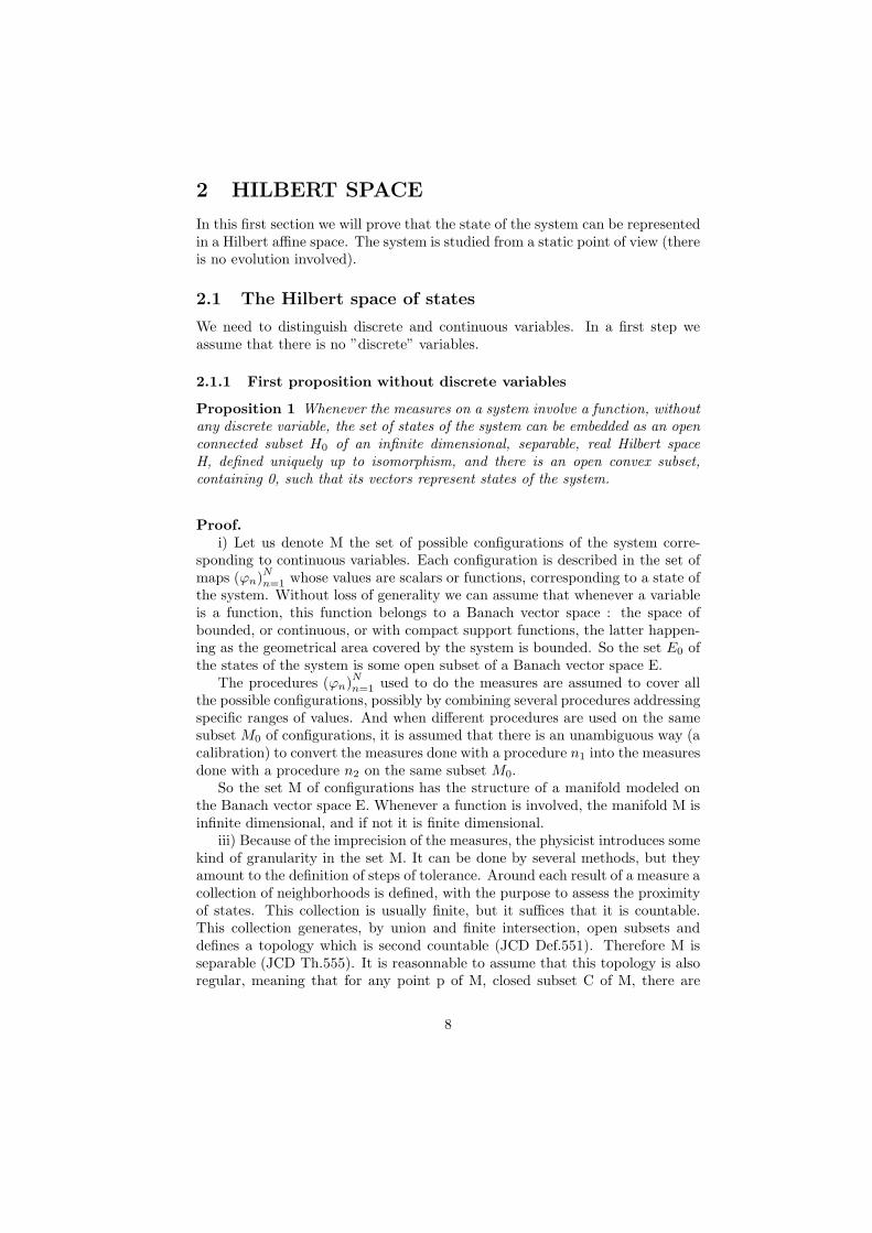
Proposition 1 Whenever the measures on a system involve a function, withoutany discrete variable, the set of states of the system can be embedded as an openconnected subset H0 of an infinite dimensional, separable, real Hilbert spaceH, defined uniquely up to isomorphism, and there is an open convex subset,containing 0, such that its vectors represent states of the system.

Proof.i) Let us denote M the set of possible configurations of the system corre-

sponding to continuous variables. Each configuration is described in the set ofmaps (ϕn)

Nn=1 whose values are scalars or functions, corresponding to a state of

the system. Without loss of generality we can assume that whenever a variableis a function, this function belongs to a Banach vector space : the space ofbounded, or continuous, or with compact support functions, the latter happen-ing as the geometrical area covered by the system is bounded. So the set E0 ofthe states of the system is some open subset of a Banach vector space E.

The procedures (ϕn)Nn=1 used to do the measures are assumed to cover all

the possible configurations, possibly by combining several procedures addressingspecific ranges of values. And when different procedures are used on the samesubset M0 of configurations, it is assumed that there is an unambiguous way (acalibration) to convert the measures done with a procedure n1 into the measuresdone with a procedure n2 on the same subset M0.

So the set M of configurations has the structure of a manifold modeled onthe Banach vector space E. Whenever a function is involved, the manifold M isinfinite dimensional, and if not it is finite dimensional.

iii) Because of the imprecision of the measures, the physicist introduces somekind of granularity in the set M. It can be done by several methods, but theyamount to the definition of steps of tolerance. Around each result of a measure acollection of neighborhoods is defined, with the purpose to assess the proximityof states. This collection is usually finite, but it suffices that it is countable.This collection generates, by union and finite intersection, open subsets anddefines a topology which is second countable (JCD Def.551). Therefore M isseparable (JCD Th.555). It is reasonnable to assume that this topology is alsoregular, meaning that for any point p of M, closed subset C of M, there are

8

open subsets O,O’ such that : p ∈ O,C ⊂ O′, O∩O′ = ∅ (JCD Def.556). Beingseparable and regular M is also metrizable (JCD Th.585). Because the number

of charts (ϕn)Nn=1 is finite E is also separable.

iv) From there the Henderson theorem states that, if M is infinite dimen-sional, it can be embedded as an open subset H0 of an infinite dimensionalseparable real Hilbert space H, defined uniquely up to isomorphism. There is acountable, locally finite, simplicial complex K such that M is homeomorphic to[K]×H . Moreover this structure is smooth and the set H−H0 is isomorphic toH, ∂H0 is homeomorphic to H0 and H0 (Henderson, JCD Th.1324). So H−H0

is connected and its complement H0 is also connected. If M is finite dimensional,say N, it can be embedded in RN which is a finite dimensional Hilbert space.And we come back to the classical picture of statistical mechanics with a finitedimensional configuration space.

v) Let us denote 〈〉 the scalar product on H (this is a bilinear symmetricpositive definite form) and ‖‖ the associated norm. The map : H0 → R :: 〈u, u〉is bounded from below and continuous, so it has a minimum u0 in H0 thatwe call a ”ground state”. By translation of H0 with u0 we can assume that 0belongs to H0. There is a largest convex subset of H which contains H0, definedas the intersection of all the convex subset contained in H0. Its interior is anopen convex subset C. It is not empty : because 0 belongs to H0 which is openin H, there is an open ball B0 = (0, r) contained in H0.

2.1.2 Complex structure

Proposition 2 The set H can be endowed with the structure of a complexHilbert space

The Hilbert space H has the structure of a real vector space. Any infinitedimensional real vector space admits, on the same set, a complex structure (JCDTh.313) J ∈ L (H ;H) : J2 = −IdH which, combined with the scalar product,can define a hermitian, definite positive sesquilinear form γ (u, v) on H, makingit a complex Hilbert space.

Proof.H has a countable hilbertian basis (εα)α∈N

because it is separable.Define :J (ε2α) = ε2α+1; J (ε2α+1) = −ε2α∀ψ ∈ H : iψ = J (ψ)So : i (ε2α) = ε2α+1; i (ε2α+1) = −ε2αThe bases ε2α or ε2α+1 are complex bases of H :ψ =

∑α ψ

2αε2α+ψ2α+1ε2α+1 =

∑α

(ψ2α − iψ2α+1

)ε2α =

∑α

(−iψ2α + ψ2α+1

)ε2α+1

‖ψ‖2 =∑

α

∣∣ψ2α − iψ2α+1∣∣2 =

∑α

∣∣ψ2α∣∣2+∣∣ψ2α+1

∣∣2+i(−ψ2α

ψ2α+1 + ψ2αψ2α+1

)

=∑

α

∣∣ψ2α∣∣2 +

∣∣ψ2α+1∣∣2 + i

(−ψ2αψ2α+1 + ψ2αψ2α+1

)

Thus ε2α is a hilbertian complex basis

9

H has a structure of complex vector space that we denote HC

The map : T : H → HC : T (ψ) =∑

α

(ψ2α − iψ2α+1

)ε2α is linear and

continuousThe map : T : H → HC : T (ψ) =

∑α

(ψ2α + iψ2α+1

)ε2α is antilinear and

continuousDefine : γ (ψ, ψ′) = g

(T (ψ) , T (ψ′)

)

γ is sesquilinearγ (ψ, ψ′) = g

(∑α

(ψ2α + iψ2α+1

)ε2α,

∑α

(ψ′2α − iψ′2α+1

)ε2α)

=∑

α

(ψ2α + iψ2α+1

) (ψ′2α − iψ′2α+1

)

=∑

α ψ2αψ′2α + ψ2α+1ψ′2α+1 + i

(ψ2α+1ψ′2α − ψ2αψ′2α+1

)

γ (ψ, ψ) = 0 ⇒ g (ψ, ψ) = 0 ⇒ ψ = 0Thus γ is definite positive

This does not impact the measures which are always supposed to be real.The complex structure is more a convenience, for mathematical purposes, thana physical requirement.

2.1.3 Second proposition including discrete variables

Proposition 3 Whenever the measures on a system involve a function, anddiscrete variables taking d values, the set of states of the system can be embeddedas d open connected subsets Hκ of an affine space, modelled on an infinitedimensional, separable, real Hilbert space H, defined uniquely up to isomorphism.

Proof.i) Now we assume that there are n discrete variables (Dk)

nk=1 and dk possible

values for each. Denoting these values by consecutive integers : 1,2,..dk thepossible configurations of the system are any combination i1, i2, .., in , ik ∈1, 2, .., dk that is a total of d=d1 × d2 × ... × dn different states. So we canconsider a single discrete variable D taking the values κ = 1, 2...d

ii) It will be convenient to represent D as a vector in Cd each value of Dbeing represented as a vector of the canonical basis of Cd.

iii) By definition the system is in one of the configurations given by the valueκ of the variable D, and the value of the other measures, which are common.Within each of these discrete configurations the previous result holds : the con-tinuous variables are represented by a vector ψ belonging to an open, connected,subset Hκ of the same Hilbert space H.

As above we translate Hκ such that the minimum of 〈u, u〉 is 0.By the Zorn lemna we can pick up any d vectors (υk)

dk=1 orthonormal to

represent the values of D by a vector ψd ∈ H .iv) We can identify a state of the system as a couple (ψd, ψ) of vectors of

H. It is convenient to define on the set (ψd, ψ) the structure of affine space Hmodelled on the Hilbert space H:

Define the map : −→ : (H ×H)× (H ×H) → H ::−−−−−−−−−−→(u, ψ) , (u′, ψ′) = ψ′ − ψ

It meets the required properties :

10

−−−−−−−−−−−−→(u1, ψ1) , (u2, ψ2) +

−−−−−−−−−−−−→(u2, ψ2) , (u3, ψ3) +

−−−−−−−−−−−−→(u3, ψ3) , (u1, ψ1) = ψ2 − ψ1 + ψ3 −

ψ2 + ψ1 − ψ3 = 0For (u, ψ) fixed, the map : τ : H → H :: τ (v) = (u, ψ + v) is a bijection.With this structure the ground states corresponding to D = κ are repre-

sented by a point Gκ with first coordinate ψd = υκ and the set of states (υκ, Hκ)

is an open subset Hκ in the hyperplane (Gκ , Hκ) .We have a collection of d

open, connected, subsets Hκ of the affine space H modelled on the Hilbert spaceH.

It is clear that this construct is quite artificial, and that many parametersare our choice. However this is a convenient representation, notably to define”subrepresentations” (related to a part of the discrete variables) and the scalarproduct of the vectors of two ground states 〈ψd, ψ′

d〉. And it fits well withthe representation used for the continuous variables. Moreover we keep theimportant property that Hκ is an open subset of the affine Hilbert space.

2.1.4 Structures involved and notations

For each non discrete measure Ξn the results belong to an open subset E0 of aBanach vector space En and E=⊕Nn=1En.

An atlas of the manifold M is given by an open cover (Oa)a∈A of M, anda collection of maps (Φa)a∈A : Φa : Oa → E where Φa = (ϕan) is a set ofmeasuring maps. The sets : Ea = Φa (Oa) are open subsets of the Banachvector space E.

The embedding of M is the diffeomorphism : ı :M → H0 ⊂ H . So the map: πa : Oa → H :: ψ = πa (xa) = ı Φ−1

a (xa) is a diffeomorphism.

M → Φ→→ E0

↓↓ ı↓H0

The manifold M has a the structure of of a smooth Hilbert manifold, sothere is an atlas such that the maps Φa, ı are smooth.

Another set of procedures(ϕ′p

)Pp=1

induces on Mκ an atlas(E, (O′

b,Φ′b)b∈B

)

which is compatible with the atlas(E, (Oa,Φa)a∈A

), and thus defines the same

structure of manifold, if and only if : ∀ (a, b) ∈ A × B,Oa ∩ O′b 6= ∅ the map

Φ′b Φ−1

a is a diffeomorphism on E′b ∩Ea. Then Hκ, H

′κ are diffeomorphic, and

H,H’ can be identified.Because ı is a diffeomorphism, a measure Ξn can be seen as a map : Ξn :

H0 → En (with the awareness that Ξn is formally defined by different, com-patible, charts, on an open cover). So in the following a chart X will be seen

as a map : X : H0 → E and the subset H0 of the affine Hilbert space H willbe called the set of states of the system. When a variable is a function, the

11

value Ξn (ψ) is a function belonging to the family of functions En with domainin some set.

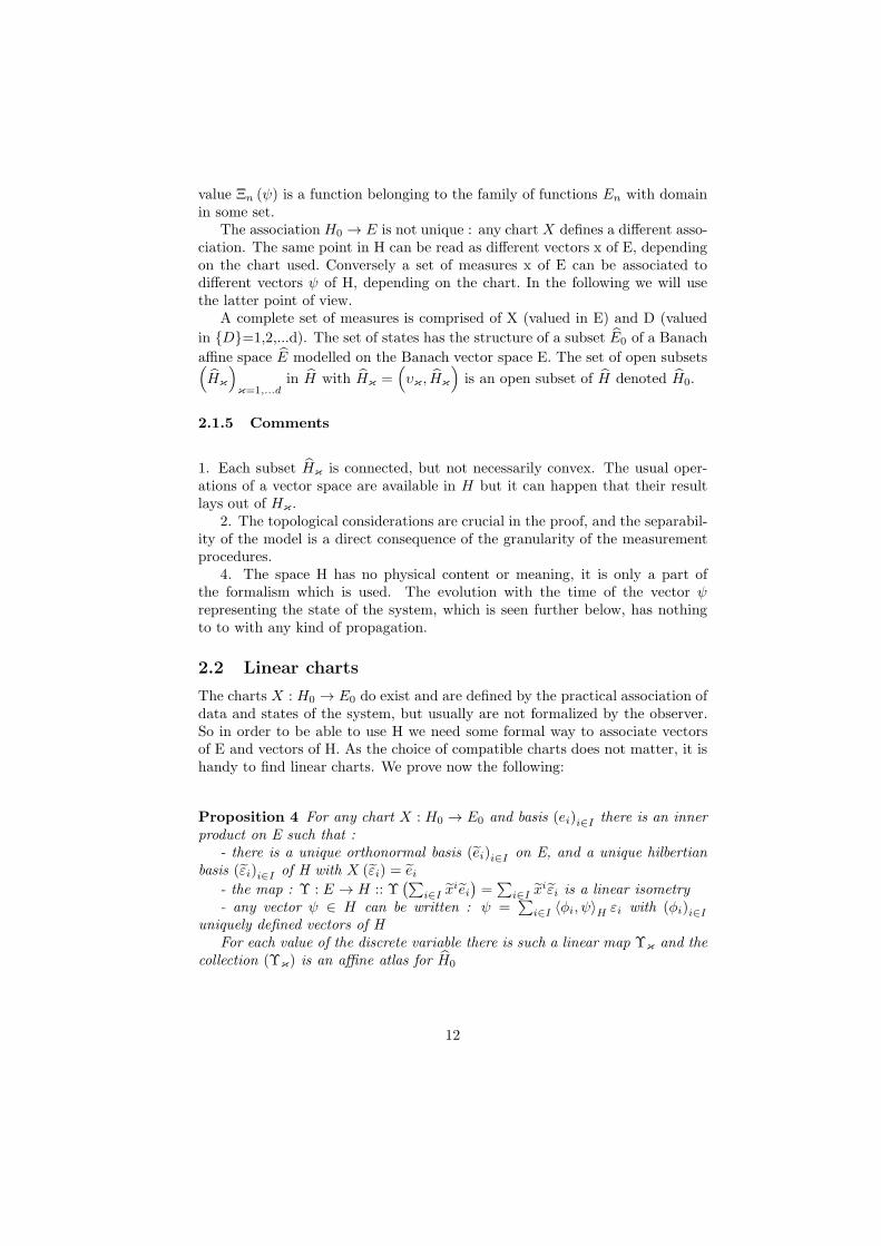
The association H0 → E is not unique : any chart X defines a different asso-ciation. The same point in H can be read as different vectors x of E, dependingon the chart used. Conversely a set of measures x of E can be associated todifferent vectors ψ of H, depending on the chart. In the following we will usethe latter point of view.

A complete set of measures is comprised of X (valued in E) and D (valued

in D=1,2,...d). The set of states has the structure of a subset E0 of a Banach

affine space E modelled on the Banach vector space E. The set of open subsets(Hκ

)κ=1,...d

in H with Hκ =(υκ, Hκ

)is an open subset of H denoted H0.

2.1.5 Comments

1. Each subset Hκ is connected, but not necessarily convex. The usual oper-ations of a vector space are available in H but it can happen that their resultlays out of Hκ .

2. The topological considerations are crucial in the proof, and the separabil-ity of the model is a direct consequence of the granularity of the measurementprocedures.

4. The space H has no physical content or meaning, it is only a part ofthe formalism which is used. The evolution with the time of the vector ψrepresenting the state of the system, which is seen further below, has nothingto to with any kind of propagation.

2.2 Linear charts

The charts X : H0 → E0 do exist and are defined by the practical association ofdata and states of the system, but usually are not formalized by the observer.So in order to be able to use H we need some formal way to associate vectorsof E and vectors of H. As the choice of compatible charts does not matter, it ishandy to find linear charts. We prove now the following:

Proposition 4 For any chart X : H0 → E0 and basis (ei)i∈I there is an innerproduct on E such that :

- there is a unique orthonormal basis (ei)i∈I on E, and a unique hilbertianbasis (εi)i∈I of H with X (εi) = ei

- the map : Υ : E → H :: Υ(∑

i∈I xiei)=∑

i∈I xiεi is a linear isometry

- any vector ψ ∈ H can be written : ψ =∑i∈I 〈φi, ψ〉H εi with (φi)i∈I

uniquely defined vectors of HFor each value of the discrete variable there is such a linear map Υκ and the

collection (Υκ) is an affine atlas for H0

12

We will use the following result (see Neeb p.60,61 and JCD Def.1155 formore) :

If F is a Hilbert space of functions : F ⊂ CE with domain any set and valuedin C or R such that the evaluation maps : ∀x ∈ E : Fx : F → C :: Fx (f) = f (x)

are continuous, then Fx ∈ F ′ (the dual of F) and has an associated vector :

Fx ∈ F : 〈Fx, f〉 = Fx (f) = f (x) and the function : K : E × E → C ::

K(x, y) = 〈Fx, Fy〉 = Fx (Fy) = Fy (x) is a positive kernel, in the meaningthat for any finite subsets (xp, yp)

np=1 the nxn matrix [K(xp, yp)] is hermitian,

positive semi-definite and |K (x, y)| ≤ K (x, x)K(y, y)Moreover if K is a positive kernel on E and X is any map : X : H → E on

any set H, then X∗K (ψ, ψ′) = K (X (ψ) , X (ψ′)) is still a positive kernel.

Proof.At first we consider the continuous variables, for a fixed value of the discrete

variables.i) The Hilbert space H has a positive definite kernel : P : H × H → C ::

P (ψ1, ψ2) = 〈ψ1, ψ2〉 . Thus, for any chart X, the function : K : Mκ ×Mκ →C :: K (X (ψ1) , X (ψ2)) = P (ψ1, ψ2) = 〈ψ1, ψ2〉 is positive definite on M, andwe have a triple (M,X−1, H) . Its canonical realization is the Hilbert space HK

of functions Kx : M → C :: Kx (y) = K (x, y) where x, y ∈ M which has forscalar product : 〈Kx,Ky〉HK

= K (x, y) =⟨X−1 (x) , X−1 (y)

⟩H

So : ∀ψx, ψy ∈ H : KX(ψx) (X (ψy)) = K (X (ψx) , X (ψy)) = 〈ψx, ψy〉 =⟨KX(ψx),KX(ψy)

⟩HK

ii) Let (ei)i∈I be any usual basis of the vector space E (so only a finitenumber of components are non null), and assuming that the vectors ei ∈ M,denote εi = X−1 (ei) ∈ H . K is definite positive and hermitian, so Kei (ej) =〈εi, εj〉 = Kij defines a positive definite hermitian sesquilinear form on E :

〈x, y〉E =∑ij∈I Kijx

iyj =∑ij∈I x

iyjK (ei, ej) =⟨∑

i∈I xiεi,∑

j∈I yjεj

⟩H

The vectors εi are linearly independant, because the determinant det [〈εi, εj〉]i,j∈Jis non null for any finite subset J of I.

Let H1 = Span (εi)i∈I be the closure of the vector subspace of H generatedby the family (εi)i∈I . This is a closed vector subspace of H, thus a Hilbert space.

By the Ehrardt-Schmidt procedure it is always possible to define an or-thonormal basis (εi)i∈I of H1 with εi = Lεi ∈ H1 defined up to a unitarytransformation U : U*U=Id : 〈Uεi, U εj〉 = 〈εi, U∗Uεj〉 = 〈εi, εj〉 .The subsetH0 contains a convex subset C of 0, thus we can assume that εi ∈ H0 and thereis ei = X (εi) which is an orthonormal basis ei = Lei of E. A vector X ∈ Ehas for coordinates in this new basis : X =

∑i∈I x

iei =∑

i∈I xiei where only

a finite number of components xi is non null.We have the following diagram :

eiX−1

→ εiL→ εi

X→ eiL−1

→ ei

X−1 L X = L

13

L, L are related :

〈ei, ej〉E = δij =([L]

∗[K] [L]

)ij

〈εi, εj〉H = δij =([L]∗

[K][L])i

j

So there is a unitary map U such that :[L]= [L] [U ] :

[U ] = [L]−1[L]⇒ [U ]

∗[U ] =

[L]∗ [

L−1]∗

[L]−1[L]

=[L]∗ [

L−1]∗ (

[L]∗ [K] [L])[L]−1

[L]=[L]∗

[K][L]= I

and it is possibe to choose (εi)i∈I such that[L]= [L] .

Then [K] = [L]∗−1

[L]−1 ⇔ [K]

−1= [L] [L]

∗

iii) The map : π : ℓ2 (I) → H1 :: πI (y) =∑i∈I y

iεi is an isomorphism ofHilbert spaces and :∀ψ ∈ H1 : ψ =

∑i∈I 〈εi, ψ〉H εi (JCD Th.1084).

Define the map : π : E → RI0 :: π(∑

i∈I xiei)=(xi)i∈I where RI0 is the

subset of the set of maps I → R such that only a finite number of componentsis non zero. It is bijective.

RI0 ⊂ ℓ2 (I) so the map : Υ = π π : E → H1 :: Υ(∑

i∈I xiei)=∑i∈I x

iεiis well defined. It is linear, injective, continuous with norm 1 with respect tothe norm induced on E by K. It preserves the scalar product :⟨∑

i∈I xiei,

∑i∈I y

iei⟩E=∑

ij∈I xiyj 〈ei, ej〉E

=∑

ij∈I xiyj 〈εi, εj〉H =

⟨Υ(∑

i∈I xiei),Υ(∑

i∈I yiei)⟩H

Thus ∀X ∈ E : xi = 〈εi,Υ(x)〉HMoreover Υ (ej) = εj :

Υ (ej) = Υ(∑

i∈I(L−1

)ijei

)=∑

i∈I(L−1

)ijεi =

∑ik∈I

(L−1

)ijLki εk =

∑k∈I

([L] [L−1

])kjεk = εj

iv) Let p be the orthogonal projection ofH on H1: ‖ψ − p (ψ)‖ = minu∈H1‖ψ − u‖

Then : ψ = p (ψ) + o (ψ) where o (ψ) ∈ H⊥1 is the orthogonal complement

of H1 :

〈εi, p (ψ) + o (ψ)〉 =⟨εi,∑

j∈I 〈εj, ψ〉H εj + o (ψ)⟩

=∑

j∈I 〈εj , ψ〉H 〈εi, εj〉+ 〈εi, o (ψ)〉 = 〈εi, ψ〉H + 〈εi, o (ψ)〉 = 〈εi, ψ〉HThere is a convex subset C of H containing 0 which is contained in H0.

There is r>0 such that : ∀ψ ∈ H : ‖ψ‖ < r ⇒ ψ ∈ H0 and as ‖ψ‖2 =

‖p (ψ)‖2 + ‖o (ψ)‖2 we have p (ψ) , o (ψ) ∈ H0.Then :∀i ∈ I : 〈εi, o (ψ)〉H = K (ei, X (o (ψ))) = 0 ⇒ X (o (ψ)) = 0 ⇒ o (ψ) = 0Thus H1 is dense in H and as it is closed H=H1 , the map Υ is an isometry

and ∀ψ ∈ H : ψ = p (ψ) ∈ H1. The basis (εi)i∈I is a hilbertian basis of H. Any

vector ψ ∈ H can be written : ψ =∑i∈I 〈εi, ψ〉H εi and

∑i∈I |〈εi, ψ〉H |2 <∞

v) For any j∈ I :

〈εi, ψ〉H εi = 〈L (εi) , ψ〉H L (εi) =∑

,jk∈I([L] [L]

∗)jk〈εj , ψ〉H εk

=∑

jk∈I

([K]−1

)jk〈εi, ψ〉H εk =

∑jk∈I

⟨([K]−1

)kjεj , ψ

⟩

H

εk

14

with [K]−1

= [L] [L]∗and [K]

∗= [K]

Let us denote : φi =∑i∈I

([K]

−1)ijεj then any vector ψ ∈ H can be

written : ψ =∑

i∈I 〈εi, ψ〉H εi =∑

i∈I 〈φi, ψ〉H εi and the series is absolutelyconvergent.

So ∀x ∈ E : Υ(∑

i∈I xiei)=∑

i∈I xiεi with x

i = 〈φi, ψ〉H .vi) The chart Υ−1 : H → E is compatible with X because X Υ : E → E ::

X Υ(∑

i∈I xiei)= X

(∑i∈I x

iεi)= X

(∑i∈I x

iεi)is a diffeomorphism.

vii) This procedure holds for any subsetHκ . D is, by construction, a bijective

map with the ground states D (Gκ) thus we have a collection (Υκ)dκ=1 of affine

maps for H0.

2.2.1 Additional results

We have additional results which are used in the following.1. For any vector of E : x =

∑i∈I x

iei where only a finite number ofcomponents xi is non null. So the series x =

∑i∈I x

iei is absolutely convergent

in the Banach space E, and because Υ is linear the series Υ(∑

i∈I xiei)=∑

i∈I xiεi is absolutely convergent in H. Conversely for any summable series∑

i∈I xiεi in H, that is :

∃ψ ∈ H : ∀ε > 0, ∃J ⊂ I, card(J) <∞, ∀K ⊂ J :∥∥∑

i∈K xiεi − ψ

∥∥ < εthe series

∑i∈I x

iei is summable in E, because ‖Υ‖ = 1 and as I is countable,both series are absolutely convergent in E (JCD Th.954)

2. We have the relations : 〈φj , εk〉 = δjk because :

〈φj , εk〉 =⟨∑

i∈I

([K]

−1)jiεi, εk

⟩=∑

i∈I

([K]

−1)ij〈εi, εk〉

=∑

i∈I

([K]−1

)ij[K]ik = δjk

2.2.2 Comments

These linear charts are crucial in the following of the paper. Some commentsare useful.

1. The structure of manifold M of the set of ”raw data” is hidden to theobserver. The chart X : H → E does exist formally, but is not known tothe observer. As for any manifold, any chart can be used to identify a pointof M. The choice of a linear chart sums up to associate to a set of measuresx =

∑i∈I x

iei a state : ψ = Υ(x) =∑i∈I x

iεi . The map Υ is uniquely definedby the chart X and the basis (ei)i∈I and ψ is uniquely defined by xi = 〈φi, ψ〉 .Of course the states ψ1 = X−1 (x) and ψ2 = Υ(x) are not the same (exceptfor x = ei) , but Υ respects the structure of manifold, through the associations

εi = X−1 (ei) and εi =∑

i,j∈I [L]ji εj which are characteristic of M.

2. The linear chart is built through an association between components ofvectors in coordinated bases in E and H. Once a basis has been decided in E,

15

the key values are the components xi , which appear both in the measurementprocess and the identification of the states in H.

The relations which occur in a change of basis are seen in the next section.3. Using the linear chart, to each vector υk is associated a vector vk =

Υ−1 (υk) ∈ E thus the condition ψd ∈ (υk)dk=1 reads Xd = Υ−1 (ψd) ∈ (vk)

dk=1

2.3 Product of systems

2.3.1 Decomposition of the Hilbert space

Proposition 5 If the model is comprised of N continuous variables (Ξk)Nk=1 ,

each belonging to a Banach vector space Ek, then the real Hilbert space H ofstates of the system is the Hilbert sum of N Hilbert space H = ⊕Nk=1Hk and anyvector ψ representing a state of the system is uniquely the sum of N vectors ψk,each image of the value of one variable Ξk in the state ψ

Proof.

By definition E =

N∏

k=1

Ek .The set E0k = 0, .., Ek, ...0 ⊂ E is a vector

subspace of E. A basis of E0k is a subfamily (ei)i∈Ik of a basis (ei)i∈I of E. E0

k

has for image by the continuous linear map Υ a closed vector subspace Hk of

H. Any vector x of E reads : x ∈N∏

k=1

Ek : x =∑N

k=1

∑i∈Ik x

iei and it has for

image by Υ : ψ = Υ(x) =∑N

k=1

∑i∈Ik x

iεi =∑Nk=1 ψk with ψk ∈ Hk .This

decomposition of Υ (x) is unique.Conversely, the family (ei)i∈Ik has for image by Υ the set (εi)i∈Ik which are

linearly independant vectors of Hk.It is always possible to build an orthonormalbasis (εi)i∈Ik from these vectors as done previously. Hk is a closed subspace of

H, so it is a Hilbert space. The map : πk : ℓ2 (Ik) → Hk :: πk (x) =∑

i∈Ik xiεi

is an isomorphism of Hilbert spaces and :∀ψ ∈ Hk : ψ =∑

i∈Ik 〈εi, ψ〉H εi.The vector subspaces Hk are orthogonal : Υ is an isometry, and∀ψk ∈ Hk, ψl ∈ Hl, k 6= l : 〈ψk, ψl〉H =

⟨Υ−1 (ψk) ,Υ

−1 (ψl)⟩E= 0

Any vector ψ ∈ H reads : ψ =∑Nk=1 πk (ψ) with the orthogonal projection

πk : H → Hk :: πk (ψ) =∑

i∈Ik 〈εi, ψ〉H εi so H is the Hilbert sum of the Hk

As a consequence the definite positive kernel of (E,Υ) decomposes as :

K ((Ξ1, ...ΞN ) , (Ξ′1, ...Ξ

′N )) =

∑Nk=1Kk (Ξk,Ξ

′k) =

∑Nk=1 〈Υ(Ξk) ,Υ(Ξ′

k)〉HThis decomposition comes handy when we have to ”translate” relations be-

tween variables into relations between vector states, notably it they are linear.But it requires that we keep the real Hilbert space structure.

2.3.2 Interacting systems

Position of the problemIn the general assumptions above the system is not necessarily isolated. If

16

there is an action of the ”outside” onto the system, this action must be accountedfor among the variables : it is subject to measures and has no special status.

If there are two systems S1,S2 which interact with each other, then one canconsider the two systems together, that is the product S1 × S2 of the models.We keep all the variables as they were, the manifold of the configuration is theproduct of the manifolds, we have a new Hilbert space, which can be identifiedto the Hilbert sum of the previous spaces, according to the result above.

However to account for the interactions, in each model of S1, S2 we need tointroduce the variables Z1, Z2 which account for the external action. It seemslogical to drop these variables, and to consider a model of the interacting systemsthat we denote S1+2 by keeping only the variables which are specific to eachsystem. We have the following diagram :

p S1 q p S2 q

X1 Z1 X2 Z2

E1 × EZ1 E2 × EZ2

H1 ⊕ HZ1 H2 ⊕ HZ2

ψ1 ψZ1 ψ2 ψZ2

p S1+2 q

X1 X2

E1 × E2

H’1 ⊕ H’2ψ′1 ψ′

2

The vector spaces E1, E2 for the definition of the variables X1, X2 specificto each system do not change. In each case the vector space to consider is theproduct : E1 × EZ1, E2 × EZ2, E1 × E2.

Using a linear map it is possible to split the vectors representing the states :H1 = Υ1 (E1 × 0) , HZ1 = Υ1 (0 × EZ1) ,H2 = Υ2 (E2 × 0) , HZ2 = Υ2 (0 × EZ2) ,H ′

1 = Υ1+2 (E1 × 0) , H ′2 = Υ1+2 (0 × E2)

This model is just the projection of S1 × S2 on E1 × E2. This always canbe done, however it is clear that we miss some important features, meaning theinteractions. So we could change the model in order to regain the informationthat we lost.

PropositionLet us denote S′

1+2 this new model. Its variable will be denoted Y, valued in aBanach vector space E’ with basis (e′i)i∈I′ . There will be another Hilbert spaceH’, and a linear map Υ′ : E′ → H ′ similarly defined. As we have the choice ofthe model, we will impose some properties to Y and E’.

a) The variables X1, X2 can be deduced from the value of Y : there must bea bilinear bijective map : Φ : E1 × E2 → E′

17

b) Φ must be such that whenever the systems S1, S2 are in the states ψ1, ψ2

then S′1+2 is in the state ψ′ and

Υ′−1 (ψ′) = Φ(Υ−1

1 (ψ1) ,Υ−12 (ψ2)

)

c) The positive kernel is a defining feature of the models, so we want apositive kernel K’ of (E′,Υ′) such that :

∀X1, X′1 ∈ E1, ∀X2, X

′2 ∈ E1 :

K ′ (Φ (X1, X2) ,Φ (X ′1, X

′2)) = K1 (X1, X

′1)×K2 (X2, X

′2)

We will prove the following :

Proposition 6 Whenever two systems S1, S2 interacts, there is a model S′1+2,

encompassing the two systems and meeting the conditions a,b,c above. It isobtained by taking the tensor product of the variables specific to S1, S2 Then theHilbert space of S′

1+2 is the tensorial product of the Hilbert spaces associated toeach system.

Proof.The map : ϕ : H1 × H2 → H ′ :: ϕ (ψ1, ψ2) = Φ

(Υ−1

1 (ψ1) ,Υ−12 (ψ2)

)is

bilinear. So, by the universal property of the tensorial product, there is a uniquemap ϕ : H1 ⊗H2 → H ′ such that : ϕ = ϕ ı where ı : H1 ×H2 → H1 ⊗H2 isthe tensorial product.

The condition iii) reads :〈Υ1 (X1) ,Υ1 (X

′1)〉H1

× 〈Υ2 (X2) ,Υ2 (X′2)〉H2

= 〈(Υ′ Φ (Υ1 (X1) ,Υ2 (X2)) ,Υ′ Φ (Υ1 (X

′1) ,Υ2 (X

′2)))〉H′

〈ψ1, ψ′1〉H1

×〈ψ2, ψ′2〉H2

= 〈ϕ (ψ1, ψ2) , ϕ (ψ′1, ψ

′2)〉H′ = 〈ϕ (ψ1 ⊗ ψ2) , ϕ (ψ′

1 ⊗ ψ′2)〉H′

The scalar products on H1, H2 extend in a scalar product on H1 ⊗ H2,endowing the latter with the structure of a Hilbert space with :

〈(ψ1 ⊗ ψ2) , (ψ′1 ⊗ ψ′

2)〉H1⊗H2= 〈ψ1, ψ

′1〉H1

〈ψ2, ψ′2〉H2

and then the reproducing kernel is the product of the reproducing kernels(JCD Th.1163).

So we must have : 〈ϕ (ψ1 ⊗ ψ2) , ϕ (ψ′1 ⊗ ψ′

2)〉H′ = 〈ψ1 ⊗ ψ2, ψ′1 ⊗ ψ′

2〉H1⊗H2

and ϕ must be an isometry : H1 ⊗H2 → H ′

So the simplest solution is to take H ′ = H1 ⊗H2 and then E′ = E1 ⊗ E2.However this solution is not unique, and indeed makes sense only if the systemsare defined by similar variables.

This proposition extends obviously for any discrete variable, thus it holdsfor any model.

3 OPERATORS

3.1 Main results

The vector space E is infinite dimensional, so an effective physical measureis a finite set of figures. And, to be consistent with the model, we define a

18

primary observable as any finite set of coordinates for a point representing astate in the affine space E0. And we distinguish continuous and discrete primaryobservables.

3.1.1 Continuous primary observables

At first we consider the case without any discrete variable. A primary observableY is a map : Y : E → E :: Y (x) =

∑j∈J x

jej where J is a finite subset of Iexpressed in some basis (ei)i∈I of E.

Main result

Proposition 7 To any physical continuous primary observable Y on the systemis associated uniquely a hermitian operator Y on H : Y = Υ Y Υ−1 with alinear chart Υ of H, such that the measure of Y, if the system is in the stateψ ∈ H0 , is Y (x) =

∑j∈J 〈φj , ψ〉 ej . Moreover Y is a compact, Hilbert-Schmidt

operator and∥∥∥YJ

∥∥∥ = 1.

We use the notations and definitions of the previous section.Proof.

i) Given any chart X and basis (ei)i∈I of E we can define a basis (εi)i∈I ofH, and the bijective, linear, maps :

π : E → RI0 :: π(∑

i∈I xiei)=(xi)i∈I where RI0 is the subset of the set of

maps I → R such that only a finite number of components is non zero.π : H → ℓ2 (I) :: π

(∑i∈I ψ

iεi)=(ψi)i∈I and ψi =

⟨φi, ψ

⟩

The linear chart Υ = π−1 π :: E → H is such that to the configuration Xis associated the state ψ with xi =

⟨φi, ψ

⟩= ψi

ii) A primary continuous observable is the selection of a finite number ofcomponents of I : YJ (X) =

∑j∈J x

jej where J is a finite subset of I.

Let us denote the map : τJ : RI0 → RI0 :: τJ

((xi)i∈I

)=(yi)i∈I where

yi = xi if i ∈ J and yi = 0 otherwise.So : YJ = π−1 τJ πiii) To the observable YJ on E we associate the operator YJ on H :

YJ = π−1 τJ π :: H → H :: YJ(∑

i∈I ψiεi)=∑

i∈J ψiεi

which reads :YJ =

(π−1 π

)(π−1 τJ π

)(π−1 π

)= Υ YJ Υ−1

EY

→→→ EJ↓ Υ ↓ Υ

H → Y→→ HJ

where EJ = Span (ei)i∈J , HJ = Υ(EJ)

19

So : YJ (ψ) =∑

j∈J 〈φj , ψ〉 εj with φj =∑i∈I

([K]−1

)ijεi and x

i =⟨φi, ψ

⟩=

ψi

This is a linear, continuous, operator. YJ depends uniquely of the basis(ei)i∈J chosen to define YJ .

YJ is a projection Y 2J = YJ and YJ is also a projection : , Y 2

J = Υ YJ Υ−1 Υ YJ Υ−1 = YJ on the vector subspace HJ .

Thus :Y 2J (ψ) =

∑j∈J

⟨φj ,∑

i∈J 〈φi, ψ〉 εi⟩εj =

∑i,j∈J 〈φi, ψ〉 〈φj , εi〉 εj =

∑j∈J 〈φj , ψ〉 εj

ii) Its adjoint Y ∗J is such that : ∀ψ, ψ′ ∈ H :

⟨YJψ, ψ

′⟩=⟨ψ, Y ∗

J ψ′⟩

A short computation gives : Y ∗J (ψ) =

∑j∈J 〈εj , ψ〉φj

Thus YJ is hermitian iff :∀ψ ∈ H :∑j∈J 〈εj , ψ〉φj =

∑j∈J 〈φj , ψ〉 εj

Expressed with respect to the independant vectors εi with [K ′] = [K]−1 and[K] = [K]

∗

YJ (ψ) =∑

j∈J∑

i∈I [K′]i

j 〈εi, ψ〉 εj =∑

j∈J∑

i∈I [K′]ji 〈εi, ψ〉 εj

Y ∗J (ψ) =

∑j∈J

∑i∈I [K

′]ij 〈εj , ψ〉 εiIf we take two vectors ψ = εp, ψ

′ = εq :

YJ (εp) =∑

j∈J

(∑i∈I [K

′]ji [K]ip

)εj =

∑j∈J δ

pj εj

Y ∗J (εp) =

∑j∈J

(∑i∈I [K

′]ij [K]jp

)εi⟨

YJεp, εq

⟩=∑

j∈J δpj 〈εj , εq〉 =

∑j∈J δ

pj [K]

jq⟨

εp, Y∗J εq

⟩=∑j∈J

(∑i∈I [K

′]ij [K]jp

)〈εp, εi〉

=∑

j∈J

(∑i∈I [K]pi [K

′]ij

)[K]jp =

∑j∈J δ

pj [K]jq

Thus YJ is hermitian on H.iii) Moreover YJ has a finite rank because YJ has a finite rank, thus YJ is a

compact operator.YJ is a Hilbert-Schmidt operator if J is a finite subset : take the Hilbertian

basis εi in H:∑

i∈I

∥∥∥YJ (εi)∥∥∥2

=∑ij∈J |〈φj , εi〉|

2 ‖εj‖2 =∑j∈J ‖φj‖

2 ‖εj‖2 <∞Because YJ is a projection, it has two eigen values : 1 and 0. The eigen space

corresponding to 1 is the vector subspace HJ generated by (εi)i∈J . Because it isa compact hermitian operator the eigen spaces corresponding to the eigen value0 is orthogonal to HJ . This is the orthogonal complement to the vector subspaceφJ generated by (φi)i∈J thus φJ = HJ and YJ is the orthogonal projection on

HJ and∥∥∥YJ

∥∥∥ = 1.

YJ is a trace class operator if J is a finite subset, with trace dimHJ∑i∈I

⟨Y (εi) , εi

⟩=∑ij∈J 〈φj , εi〉 〈εj , εi〉 =

∑ij∈J φ

ijεij

=∑

j∈J 〈φj , εj〉 =∑j∈J

∑k∈I [K

′]k

j 〈εk, εj〉=∑

j∈J∑

k∈I [K′]jk [K]

kj =

∑j∈J δjj = dimHJ

20

iv) Any vector of H can be written ψ =∑

i∈I ψiεi and the vectors εi ∈ H0.

Thus the image YJ (ψ) =∑

j∈J ψjεj ∈ HJ ⊂ H0 if ψ ∈ H0 and the operators

are well defined as maps : H0 → HJ .

Further properties of continuous observables1. As any vector ψ ∈ H can be written : ψ =

∑i∈I 〈φi, ψ〉 εi the series :

YJ (ψ) =∑

i∈J 〈φi, ψ〉 εi is still convergent for any subset J of I, even infiniteand we denote HJ the closure of Span(εj , j ∈ J). In the following we will precisewhen J is finite.

2. Any primary observable can be written : YJ (ψ) =∑

j∈J φj (ψ) εj where

φj ∈ E′ is the 1-form associated to φj such that φj (ψ) ∈ R

3. As εj =[L−1

]ijεi, φj =

∑i∈I

([K]

−1)ijεi =

∑i∈I

([K]

−1)ij

[L−1

]kiεk =

∑k∈I

([L]

∗)kjεk with [K]

−1= [L] [L]

∗

YJ (ψ) =∑

j∈J,kl∈I

⟨([L]

∗)kjεk, ψ

⟩ [L−1

]ljεl =

∑j∈J,kl∈I ([L])

jk

[L−1

]lj〈εk, ψ〉 εl

So : YJ (ψ) =∑

kl∈I Akl 〈εk, ψ〉 εl where Akl =

∑j∈J

[L−1

]lj[L]

jk∥∥∥YJ (ψ)

∥∥∥2

=∑

kl∈I∣∣Akl

∣∣2∣∣∣ψk∣∣∣2

≤∑k∈I

∣∣∣ψk∣∣∣2

3.1.2 Discrete primary observables

Main result

Proposition 8 To any primary observable DJ on the discrete variables is as-sociated a continuous, hermitian operator DJ in the Hilbert space H wich reads: DJ (ψd) =

∑dm=1 〈ϑm, ψd〉 υm with (υk)

dk=1 an orthonormal family of vectors

of H and (ϑk)dk=1 vectors of H which are linearly independant iff the observable

involves all the discrete variables. DJ (ψd) corresponds to a unique point in the

affine space H belonging to H0 iff all the discrete variables are involved.

Proof.i) Using the notations of the first section, we have n discrete variables

(Dk)nk=1 taking their values in 1, 2, ..., dk which have been synthetized in the

single discrete variable D taking its values in 1, 2, ..., d and represented by

one the vectors of a basis (eκ)dκ=1 of Cd . The value

−→D = eκ corresponds to

some combination (i1, i2, .., in) , ik ∈ 1, .., dk of each the Dk. A reduced ob-servable DJ is a set of discrete variables (Dk)k∈J . It takes its values in a subset(iα1

, iα2, .., iαn

) , αk ∈ 1, ..n of the values of D, values which are labelled 1,2,..s.To a given value κJ of DJ correspond several values of D.

Let us denote : Aji = 1 if D = i ⇒ DJ = j and Aji = 0 otherwise. Thes × d matrix [A] has rank s (the states measured by DJ are all distinct) andhas exactly one 1 in each column. The measure of DJ can be represented as

21

a projection of the same vector−→D on a smaller orthogonal basis (κk)

sk=1of C

d

built from (eκ)dκ=1 :

l=1...s : κj =∑d

κ=1 [A]jκeκ and [A] [A]

t= Is×s

Similarly in H the vector ψd representing a state of the system is projectedon a smaller basis (k)

sk=1, built from (υk)

dk=1 : l=1...s : j =

∑dk=1 [A]

jk υk

ii) The operator becomes : DJ : H → H :: DJ (ψd) =∑s

j=1 〈j , ψd〉 j. Itreads :

DJ (ψd) =∑s

j=1 〈j , ψd〉 j =∑s

j=1

⟨∑dk=1 [A]

jk υk, ψd

⟩(∑dl=1 [A]

jl υl

)

=∑s

j=1

∑dk,l=1 [A]

jk [A

t]lj 〈υk, ψd〉 υl

=∑d

k,l=1

([A]t [A]

)lk〈υk, ψd〉 υl =

∑dl=1 〈ϑl, ψd〉 υl

DJ (ψd) =∑d

j=1 〈ϑj , ψd〉 υj with ϑj =∑d

k=1

([A]

t[A])jkυk

By permutation of the columns the matrix [A] can be put in the form [AJ ]of exactly d/s copies of the unit s × s matrix, which can be written : [AJ ] =[P ] [A] ⇔ [A] = [P ]

t[AJ ] where [P ] is a permutation matrix. So [A]

t[A] =(

[AJ ]t[P ])[P ]

t[AJ ] = [AJ ]

t[AJ ] is a d x d matrix, of rank s, made of copies of

the unit sxs matrix I and its main diagonal has 1 for elements. So the vectors(ϑj)

dj=1 are actuallly d/s copies of the collection of s vectors ϑj .

They are orthonormal : 〈ϑi, ϑj〉 =⟨∑d

k=1

([A]

t[A])ikυk,∑dk=1

([A]

t[A])jkυk

⟩

=∑d

k=1

([A]

t[A])ik

([A]

t[A])jk=([A]

t[A] [A]

t[A])ij=([A]

t[A])ij= δij

The value for ψd = υκ is :DJ (ψd) =

∑sj=1 〈j, υκ〉 j =

∑sj=1 [A]

jκj and only one coefficient [A]

jκis

non zero.iii) DJ is linear, thus continuous and hermitian.

Indeed its adjoint(DJ

)∗is such that :

⟨DJ (ψd) , ψ

′d

⟩=⟨ψd,(DJ

)∗ψ′d

⟩

that is :[(DJ

)∗]=[DJ

]∗=([A]

t[A])∗

=([A]

t[A])t

= [A]t[A] because

[A] is real.It is a projection on the vector subspace spanned by (k)

sk=1

DJ (k) =∑s

j=1 〈j , k〉 j = k

D2J (ψd) = DJ

(∑sj=1 〈j, ψd〉 j

)=∑s

j=1 〈j , ψd〉 DJ (j) = DJ (ψd)

Examplewith D1 = 1, 2 , D2 = 1, 2, 3 restricted to D2

υ1 ↔ (1, 1) , υ2 ↔ (1, 2) , υ3 ↔ (1, 3) , υ4 ↔ (2, 1) , υ5 ↔ (2, 2) , υ6 ↔ (2, 3) ,1 = (υ1 + υ4) , 1 = (υ2 + υ5) , 3 = (υ3 + υ6)

22

A =

1 0 0 1 0 00 1 0 0 1 00 0 1 0 0 1

[A]t[A] =

1 0 00 1 00 0 11 0 00 1 00 0 1

1 0 0 1 0 00 1 0 0 1 00 0 1 0 0 1

=

1 0 0 1 0 00 1 0 0 1 00 0 1 0 0 11 0 0 1 0 00 1 0 0 1 00 0 1 0 0 1

[A] [A]t=

1 0 0 1 0 00 1 0 0 1 00 0 1 0 0 1

1 0 00 1 00 0 10 0 00 0 00 0 0

=

1 0 00 1 00 0 1

Further properties of the discrete operators1. As a point in the set of states is defined by a couple of vectors (ψd, ψ) a

primary observable (DJ , YJ′) gives a couple of maps(DJ , YJ′

)on HxH and the

image of a point in the affine space H is a point in H.2. The operator is a projection, its eigen values are (0,1) and the vector

subspace spanned by (k)sk=1 corresponds to the eigen value 1.

3. The operators associated to different discrete observables commute :

DJ DJ′ (ψd) =∑d

m=1

⟨ϑm,

∑dp=1

⟨ϑ′p, ψd

⟩υp

⟩υm

=∑d

m=1

∑dp=1

⟨ϑ′p, ψd

⟩〈ϑm, υp〉 υm

=∑d

m=1

∑dp=1

⟨∑dl=1

([A′]t [A′]

)plυl, ψd

⟩⟨∑dk=1

([A]

t[A])mkυk, υp

⟩υm

=∑d

m=1

∑dp=1

∑dl=1

([A′]t [A′]

)pl

∑dk=1

([A]

t[A])mk〈υl, ψd〉 〈υk, υp〉 υm

=∑d

m=1

∑dk,l=1

([A]

t[A])mk

([A′]t [A′]

)kl〈υl, ψd〉 υm

=∑d

l,m=1

([AJ ]

t [AJ ] [A′J ]t[A′J ])ml〈υl, ψd〉 υm

The product of matrices comprised of unit submatrices commute :[AJ ]

t[AJ ] [A

′J ]t[A′J ] = [A′

J ]t[A′J ] [AJ ]

t[AJ ]

So DJ1 DJ2

= DJ2 DJ1

However the result is not necessarily an operator of the kind DJ for some J.

3.2 Secondary continuous observables

From primary continuous observables, which are the just basic measures thatcan be done on the system, we can define secondary observables, which arevariables defined through the combination of primary observables.

23

3.2.1 Algebra of primary continuous observables

The simplest combination of primary observables is through an algebra, meaningby linear combination and composition of primary observables.

Proposition 9 The operators associated to the projection of each vector ei ofa basis of E are a set of orthogonal operators, and are the generators of acommutative C*-subalgebra A of L(H ;H) and a Hilbert space.

Proof.i) For each j∈ I we have the primary operator : Yj (ψ) = φj (ψ) εj =

〈φj , ψ〉 εj with φj the 1-form associated to φj

Yj =∑

kl∈I Akl εk ⊗ εl where A

kl =[L−1

]lj[L]

jk

This is the projection of ψ on the vector εj of the (non hilbertian) basis(εj)j∈I .

The primary operators(Yj

)j∈I

are mutually orthogonal :

Yj Yk (ψ) = 〈φk, ψ〉 〈φj , εk〉 εj = 〈φk, ψ〉∑

i∈I[K−1

]ji[K]

ik εj = δjkYj (ψ)

Any primary observable can be written :YJ (ψ) =

∑j∈J Yj (ψ) and

∑j∈I Yj (ψ) = ψ

YJ1 YJ2

= YJ1∩J2= YJ2

YJ1

YJ1∪J2= YJ1

+ YJ2− YJ1∩J2

= YJ1+ YJ2

− YJ1 YJ2

Notice that⟨Yj1ψ, Yj2ψ

⟩6= 0 usually :

⟨Yj1ψ, Yj2ψ

⟩=⟨ψj1εj1,ψ

j2εj2,⟩= [K]

j1j2ψj1ψj2

ii) Denote Y0 = I where I is the identity on H and I0 = I ∪ 0For any family

(ui)i∈I0 ∈ CI0 ,maxi∈I0

∣∣ui∣∣ < ∞ the endomorphism : Y =

∑i∈I0 u

iYi is well defined and ‖Y ‖ = supi∈I0∣∣ui∣∣

Define A as the set of endomorphismsA =Y =

∑i∈I0 u

iYi,(ui)i∈I0 ∈ ℓ2 (I0)

A has the structure of a commutative C*-subalgebra of L(H ;H) with com-position as internal operation :(∑

i∈I0 uiYi

)(∑

i∈I0 viYi

)=∑i∈I0 u

iviYi

A has the structure of a Hilbert space with the scalar product : 〈Y1, Y2〉A =∑i∈I0 u

i1ui2 and

(Yi

)i∈I0

is a Hilbertian basis.

Moreover :1. The adjoint of Y =

∑i∈I u

iYi is Y∗ =

∑i∈I u

iYi and the elements of A

are normal : Y Y ∗ =∑

i∈I0∣∣ui∣∣2 Yi

Any element of A is compact, because it is the limit of the sequence of finiterank maps Yi

It is Hilbert-Schmidt because the space of Hilbert-Schmidt operators is aHilbert space.

24

The eigen values and eigen vectors of Y =∑i∈I u

iYi are(ui, εi

)i∈I

The eigen values and eigen vectors of (Y Y ∗)1/2 =∑

i∈I∣∣ui∣∣ Yi are

(∣∣ui∣∣ , εi

)i∈I .

If they are summable∑i∈I∣∣ui∣∣ <∞ then Y is trace-class (JCD Th.1115).

2. Each vector ψ ∈ H defines the continuous linear functional on A :

ϕψ : A→ C :: ϕψ (Y ) = 〈Y ψ, ψ〉 =⟨∑

i∈I uiYi(∑

k∈I ψkεk),∑j∈I ψ

jεj

⟩=

∑i,j∈I u

iψi[K]

ij ψ

j = [uψ]∗[K] [ψ]

ϕψ is hermitian(ϕψ (Y ∗) = ϕψ (Y )

)and positive (ϕψ (Y Y ∗) ≥ 0) .

Such linear functionals are called ”states” in the usual algebraic formulationof QM.

3. To the operator Y =∑i∈I0 u

iYi where(ui)i∈I0 ∈ R

I00 (only a finite

number of coefficients is non zero), is associated the observable on E : Y =∑i∈I0 u

iYi which is valued in a finite dimensional subspace of E.

3.2.2 Secondary continuous observables on H

We can go further, but we need two general lemna.

Lemma 10 There is a bijective correspondance between the projections on aHilbert space H, meaning the operators

P ∈ L (H ;H) : P 2 = P, P = P ∗

and the closed vector subspaces HP of H. And P is the orthogonal projectionon HP

Proof.i) If P is a projection, it has the eigen values 0,1 with eigen vector spaces

H0, H1. They are closed as preimage of 0 by the continuous maps : Pψ =0, (P − Id)ψ = 0

Thus : H = H0 ⊕H1

Take ψ ∈ H : ψ = ψ0 + ψ1

〈P (ψ0 + iψ1) , ψ0 + ψ1〉 = 〈iψ1, ψ0 + ψ1〉 = −i 〈ψ1, ψ0〉 − i 〈ψ1, ψ1〉〈ψ0 + iψ1, P (ψ0 + ψ1)〉 = 〈ψ0 + iψ1, ψ1〉 = 〈ψ0, ψ1〉 − i 〈ψ1, ψ1〉P = P ∗ ⇒ −i 〈ψ1, ψ0〉 = 〈ψ0, ψ1〉〈P (ψ0 − iψ1) , ψ0 + ψ1〉 = 〈−iψ1, ψ0 + ψ1〉 = i 〈ψ1, ψ0〉+ i 〈ψ1, ψ1〉〈ψ0 − iψ1, P (ψ0 + ψ1)〉 = 〈ψ0 − iψ1, ψ1〉 = 〈ψ0, ψ1〉+ i 〈ψ1, ψ1〉P = P ∗ ⇒ i 〈ψ1, ψ0〉 = 〈ψ0, ψ1〉〈ψ0, ψ1〉 = 0 so H0, H1 are orthogonalP has norm 1 thus ∀u ∈ H1 : ‖P (ψ − u)‖ ≤ ‖ψ − u‖ ⇔ ‖ψ1 − u‖ ≤ ‖ψ − u‖

and minu∈H1‖ψ − u‖ = ‖ψ1 − u‖

So P is the orthogonal projection on H1 and is necessarily unique.ii) Conversely any orthogonal projection P on a closed vector space meets

the properties : continuity, and P 2 = P, P = P ∗

25

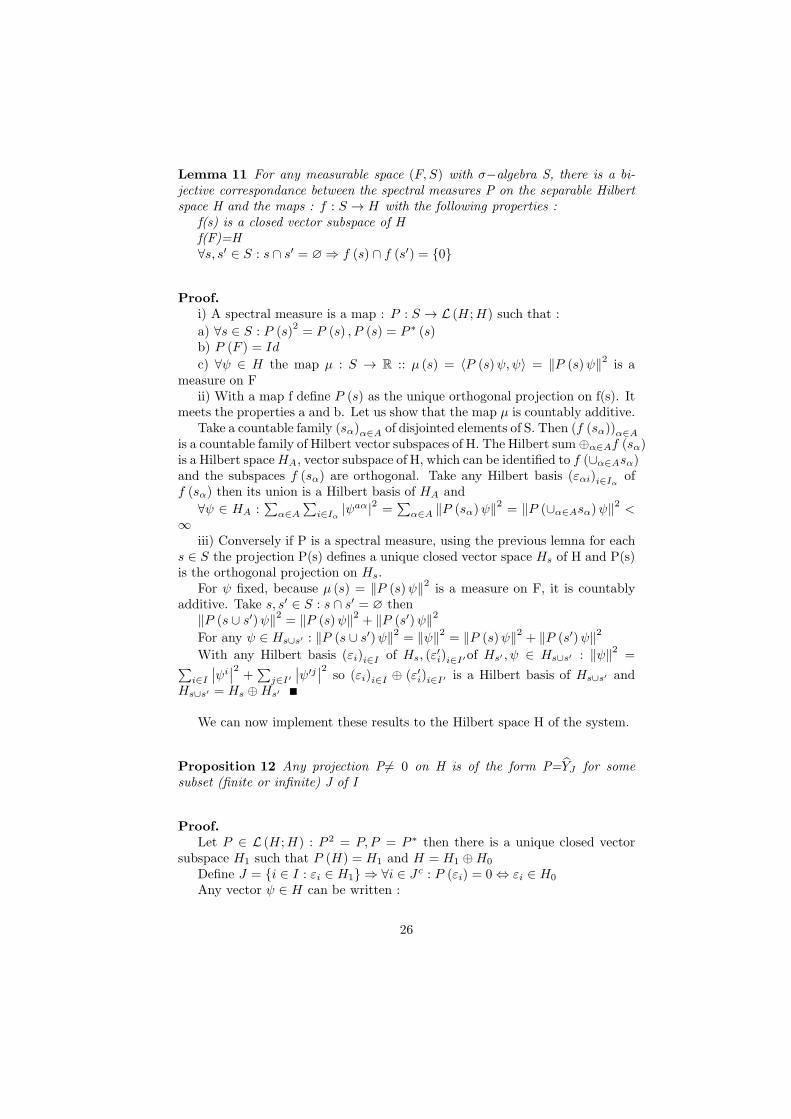
Lemma 11 For any measurable space (F, S) with σ−algebra S, there is a bi-jective correspondance between the spectral measures P on the separable Hilbertspace H and the maps : f : S → H with the following properties :

f(s) is a closed vector subspace of Hf(F)=H∀s, s′ ∈ S : s ∩ s′ = ∅ ⇒ f (s) ∩ f (s′) = 0

Proof.i) A spectral measure is a map : P : S → L (H ;H) such that :

a) ∀s ∈ S : P (s)2= P (s) , P (s) = P ∗ (s)

b) P (F ) = Id

c) ∀ψ ∈ H the map µ : S → R :: µ (s) = 〈P (s)ψ, ψ〉 = ‖P (s)ψ‖2 is ameasure on F

ii) With a map f define P (s) as the unique orthogonal projection on f(s). Itmeets the properties a and b. Let us show that the map µ is countably additive.

Take a countable family (sα)α∈A of disjointed elements of S. Then (f (sα))α∈Ais a countable family of Hilbert vector subspaces of H. The Hilbert sum⊕α∈Af (sα)is a Hilbert spaceHA, vector subspace of H, which can be identified to f (∪α∈Asα)and the subspaces f (sα) are orthogonal. Take any Hilbert basis (εαi)i∈Iα off (sα) then its union is a Hilbert basis of HA and

∀ψ ∈ HA :∑α∈A

∑i∈Iα |ψaα|2 =

∑α∈A ‖P (sα)ψ‖2 = ‖P (∪α∈Asα)ψ‖2 <

∞iii) Conversely if P is a spectral measure, using the previous lemna for each

s ∈ S the projection P(s) defines a unique closed vector space Hs of H and P(s)is the orthogonal projection on Hs.

For ψ fixed, because µ (s) = ‖P (s)ψ‖2 is a measure on F, it is countablyadditive. Take s, s′ ∈ S : s ∩ s′ = ∅ then

‖P (s ∪ s′)ψ‖2 = ‖P (s)ψ‖2 + ‖P (s′)ψ‖2For any ψ ∈ Hs∪s′ : ‖P (s ∪ s′)ψ‖2 = ‖ψ‖2 = ‖P (s)ψ‖2 + ‖P (s′)ψ‖2With any Hilbert basis (εi)i∈I of Hs, (ε

′i)i∈I′of Hs′ , ψ ∈ Hs∪s′ : ‖ψ‖2 =

∑i∈I∣∣ψi∣∣2 +

∑j∈I′

∣∣ψ′j∣∣2 so (εi)i∈I ⊕ (ε′i)i∈I′ is a Hilbert basis of Hs∪s′ andHs∪s′ = Hs ⊕Hs′

We can now implement these results to the Hilbert space H of the system.

Proposition 12 Any projection P6= 0 on H is of the form P=YJ for somesubset (finite or infinite) J of I

Proof.Let P ∈ L (H ;H) : P 2 = P, P = P ∗ then there is a unique closed vector

subspace H1 such that P (H) = H1 and H = H1 ⊕H0

Define J = i ∈ I : εi ∈ H1 ⇒ ∀i ∈ Jc : P (εi) = 0 ⇔ εi ∈ H0

Any vector ψ ∈ H can be written :

26

ψ =∑

i∈I 〈φi, ψ〉H εi ⇒ P (ψ) =∑i∈J 〈φi, ψ〉H εi = YJ (ψ)

Notice that H1 can be infinite dimensional.

Proposition 13 For any measured space (F, S) with σ−algebra S, there is abijective correspondance between the spectral measures P on the Hilbert space Hand the maps : χ : S → 2I such that χ (F ) = I and ∀s, s′ ∈ S : s ∩ s′ = ∅ ⇒χ (s) ∩ χ (s′) = ∅. The spectral measure is then P (s) = Yχ(s)

Proof.i) Let P be a spectral measure. Then there is a map : f : S → H such thatf(s) is a closed vector subspace of Hf(F)=H∀s, s′ ∈ S : s ∩ s′ = ∅ ⇒ f (s) ∩ f (s′) = 0For s fixed, P(s) is a projection so ∃χ (s) ⊂ I : P (s) = Yχ(s) and f(s)=Yχ(s) (H)

P (F ) = Id = YI ⇔ χ (F ) = I∀s, s′ ∈ S : s ∩ s′ = ∅ ⇒f (s) ∩ f (s′) = 0 ⇔ Yχ(s) (H) ∩ Yχ(s′) (H) = 0 ⇔ χ (s) ∩ χ (s′) = ∅

ii) Conversely, to any map χ : S → 2I let us associate the map :

f (s) = Yχ(s) (H)

This is a closed vector subspace of H, f(F)=YI (H) = H,

∀s, s′ ∈ S : s ∩ s′ = ∅ ⇒ f (s) ∩ f (s′) = Yχ(s) (H) ∩ Yχ(s′) (H) = 0

As a consequence for any fixed ψ ∈ H, ‖ψ‖ = 1, the function µ : S → R ::

µ (s) =⟨Yχ(s)ψ, ψ

⟩=∥∥∥Yχ(s)ψ

∥∥∥2

is a probability law on (F,S). Which implies

that : ∀s, s′ ∈ S : s ∩ s′ = ∅ :∥∥∥Yχ(s+s′)ψ

∥∥∥2

=∥∥∥Yχ(s)ψ

∥∥∥2

+∥∥∥Yχ(s′)ψ

∥∥∥2

From there we have the following results :

Theorem 14 For any measured space (F, S) with σ−algebra S, any map : χ :S → 2I and bounded measurable function f : F → R , the spectral integral:∫F f (ξ) Yχ(ξ) defines a continuous operator on H. Moreover for any map χ

this procedure gives a representation of the C*algebra of the bounded measurablefunctions Cb (F ;R) and its image is a C*subalgebra of L(H ;H) .

This is an application of standard theorems on spectral measures (JCD Th1192, 1197):

The spectral integral is such that there is an operator denoted ϕ =∫Ff (ξ) Yχ(ξ)

with :∀ψ, ψ′ ∈ H : 〈ϕ (ψ) , ψ′〉 =

∫Ff (ξ)

⟨Yχ(ξ) (ψ) , ψ

′⟩

To this operator one can associate the secondary observable on E :

27

Φ : E → E :: Φ = Υ−1 ϕ ΥΦ(x) =

∫F f (ξ)Yχ(ξ) (x) =

∫F f (ξ)

(∑j∈χ(ξ) x

jej

)∈ L (E;E)

Theorem 15 For any continuous normal operator ϕ on H, there is a map :χ : Sp(f) → 2I such that : ϕ =

∫Sp(f)

sYχ(s) where Sp(f) is the spectrum of f.

If ϕ has finite range then it belongs to the algebra A (see previous subsection).

Proof.i) The first part is the direct application of a classic of spectral analysis

(JCD Th.1197). ϕ has a spectral resolution and so there is a map χ with theproperties above.

ii) If ϕ has a finite range it is necessarily compact, and χ (s) must be a finitesubset of I. By the Riesz theorem (JCD Th.1106) the spectrum of ϕ is eitherfinite or is a countable sequence converging to 0, contained in disc of radius‖ϕ‖ and is identical to the set (λn)n∈N

of its eigen values (JCD Th.973). Foreach eigen value λ (except possibly 0), the eigen spaces Hλ are orthogonal fordistinct eigen values.

Thus :as ϕ has finite range the set (λn)

Nn=1 of its distinct eigen values is finite

Jn = χ (λn) ⊂ I

Hn = Yχ(λn) (H) = HJn

for n 6= n′ : Jn 6= Jn′

For each distinct eigen value λn let (ψnm)Nn

m=1 be an orthonormal basis ofHn. Then ϕ reads :

ϕ (ψ) =∑N

n=1 λn∑Nn

m=1 〈ψnm, ψ〉ψnm and also : ϕ =∑Nn=1 λnYJn

whereJn = χ (λn) .

So ϕ ∈ A and for each n the eigen vectors ψnm are a linear combination ofthe (εj)j∈Jn

To ϕ one can associate the observable : Φ : E → E :: Φ = Υ−1 ϕ ΥΦ(x) =

∑Nn=1 λnYχ(λn) (x)

As seen above, the operator is self adjoint iff the eigen values are real, thatis if Φ takes real values.

The probability law on the set of eigen values reads, for a vector ψ ∈H, ‖ψ‖ = 1 fixed :

µn =⟨YJn

(ψ) , ψ⟩=∥∥∥YJn

ψ∥∥∥2

=∑Nn

m=1 |〈ψnm, ψ〉|2

3.2.3 Product of observables

1. Secondary observables such as Φ (x) =∑Nn=1 λnYχ(λn) (x) or

∫F f (ξ)Yχ(ξ)

can be formally defined, but we need to precise how their value can be measured.This can be conceived in two ways :

- either one proceeds at first to the measure of the primary observables andthen to the computation according to the previous formulas

28

- or, because the result is still a vector of E, their value is measured throughanother primary observable. This procedure is then modeled as the composition: YJ Φ which translates as YJ ϕ for some finite subset J of I.

The second options seems the more logical, and anyway the only practicalwhenever the secondary observable is defined through a continuous spectrum.

The product gives :YJ ϕ =

∑Nn=1 λnYχ(λn)∩J in the first case and the subsets χ (λn) ∩ J are

disjointedYJ ϕ =

∫Ff (ξ)Yχ(ξ)∩J in the second case

So, in both cases, it sums up actually to restrict the scope of χ (λn) , χ (ξ)to finite subsets.

In the first case the finite collection of finite disjointed sets (χ (λn))Nn=1 is a

finite subset Jϕ of I. To make sense the measure by YJ should encompass onlythe indices in Jϕ and this is possible. Then the result is just ϕ.

2. The product of two secondary observables has no clear meaning in thispicture, and it is not necessary to define the observables on the system. So itdoes not play a significant role in the following.

3.2.4 Scalar functions

In the previous cases the secondary observables are continuous variables whichare either scalars or tensors defined over the whole of the system, or localizedmaps. In particular Φ (x) can be the Fourier transform of a map on E.

One can also consider continuous maps : λ : E → R meaning belongingto the dual E’ of E. They induce a map in H : λ = λ Υ−1 ∈ H ′ which isrepresented by a vector φ ∈ H : λ (ψ) = 〈φ, ψ〉 = λ Υ−1 (ψ) .

As a special case one can consider the vectors (υk)Nk=1 of H, which are an

arbitrary family of orthonormal vectors. They can always be chosen such that: 〈υk, ψ〉 = λk Υ−1 (ψ) = λk (X (ψ)) which can be useful if the variables aresubject to a constraint expressed by an integral.

3.3 Probability

3.3.1 Preliminaries

The formalism developped so far is strictly determinist : to any set of measures(a configuration) corresponds a unique point in the Hilbert affine space. Howeverthere is a natural physical probabilist interpretation of some results. But itis necessary at first to make the distinction between formal probability andphysical probability.

A probability law is, in mathematics, a positive measure P on some mea-surable space (F,S) such that P(S)=1. So, for any spectral measure P on a

measurable space (F,S) and vector ψ ∈ H, the map : µ : S → R :: ‖P (s)ψ‖2 isformally a probability law, meaning that it is positive, countably additive and

29

µ (F ) = 1. But these properties are not in any way related to a physical event,which could or not occur and could be reasonably governed by a probability.

Probability in physics may appear either because the model introduces ran-dom variables (the physical phenomenon being determinist or not) or throughthe process of measures itself. In our picture the second case is explicit. Theprecision of the measures is involved in two ways :

- by the uncertainty of any measure, which is controled by a protocol inorder to validate the results

- by the fact that we estimate functions from a finite set of dataIn our picture the knowledge of the state represented by (ψd, ψ) can be seen

as the purpose of the measures. If we knew the values of all the variables,we would know precisely the state. But these variables are functions, definedby infinitely many parameters, which are the components (xi)i∈I .Moreover,usually the basis (ei)i∈I and the indices i are not known by the physicist : weknow that they exist from their mathematical definition, but the functions areestimated by statistical methods from one batch of finite measures. For instancethe simplest way to estimate a function is to use a linear interpolation from asample of points. To do so, one does not need to know the basis, but actually theprocedure is legitimate because this basis does exist. Because the estimationsuse controled statistical methods, the uncertainty on the estimates is known. Itdepends on the nature of the variables which are measured, and on the numberof measures which are done.

3.3.2 Main result

Proposition 16 When the measure of the continuous variables is done accord-ing to a precision protocol, any measure of a state ψ ∈ H of the system has theprobability ν (J) of belonging to YJ (H) . ν is a physical probability law on the

measurable space (I,2I) and if ‖ψ‖ = 1 then∥∥∥YJ (ψ)

∥∥∥2

= ν (J) = Pr (ψ ∈ HJ)

Proof.i) To estimate the configuration X =

∑i∈I y

iei one uses a batch of datawhich can be summarized as the primary observable : YJ =

∑i∈J y

iei for afinite set J of I. Let us denote EJ the vector subspace generated by (ei)i∈J andσ (EJ ) its Borel σ−algebra. The uncertainty on the measure of X is : oJ (Y ) =∑i∈Jc yiei which can take any value in EJc . Because the estimation is done

using controlled statistical methods, some rules are implemented to quantify theuncertainty of the measure. We assume that the protocol used is such that :

a) For any finite subset J of I, there is a positive, finite, measure µJ onthe Borel σ−algebra of EJc such that the probability Pr (X − YJ (X) ∈ J) isµJ (J) , with µJ (EJc) = 1.

b) This measure does not depend of the order of the indices in the collectionJ

30

c) For any finite subsets J,K of I, J ∈ σ (EJc) :µJ∪K (Jc ∪ EKc) = µJ (Jc)Then by the Kolomogorov theorem (JCD Th.816) the collection of measures

µJ can be uniquely extended to a measure µ on E such that µ (J) = µJ (J) .And µ (E) = 1.

ii) This measure has for image in the Hilbert space H by the linear mapΥ a finite, positive, measure µ on the Borel σ−algebra σH of H such that theprobability that o (ψ) = ψ − YJ (ψ) ∈ is given by µ () . And µ (H) = 1.

Let us denoteHJ = YJ (H) and ν (J) = 1−µ (HJ) . The set 2I is a σ−algebra

of I and ν (J) is a finite, positive measure on (I,2I).The physicist can see (meaning measure) only states belonging to the vector

subspaces HJ , so one can interpret the previous probability the other wayaround. Whatever the state of the system, the probability that the result of themeasure belongs to HJ is ν (J) . The probability increases with J and is 1 if J=I,but the measure is not necessarily absolutely continuous, so the probability forJ=j is not necessarily null. As one can access only to the states belonging toHJ , for J finite, for all that matters, ν (J) can be interpreted as the probabilitythat ψ belongs to HJ .

iii) Take any fixed vector ψ ∈ H, ‖ψ‖ = 1 then : 0 ≤∥∥∥YJ (ψ)

∥∥∥2

≤ 1. It is 0

if ψ ∈ HJc and 1 if ψ ∈ HJ .∥∥∥YJ (ψ)∥∥∥2

can be seen as a random variable, the value of which is the product

of the value of ‖ψ‖2 if ψ ∈ HJ by the probability that ψ ∈ HJ

Thus :∥∥∥YJ (ψ)

∥∥∥2

= ν (J) and one can write :∥∥∥YJ (ψ)

∥∥∥2

= ν (J) =

Pr (ψ ∈ HJ )

Comments1. Let us take a single continuous variable x, which takes its values in R. It is

clear that any physical measure will at best give a rational number Y (x) ∈ Q upto some scale. There are only countably many rational numbers for unacount-ably many real scalars. So the probability to get Y (x) ∈ Q should be zero.The simple fact of the measure gives an incommensurable weigth to rationalnumbers, implying that each of them has some small, but non null, probabilityto appear. In this case I can be assimilated to Q , the subsets J are any finitecollection of rational numbers.

2. The experimental proof of some theoretical statements can be deceptive.If a physicist states ”the ratio of the circumference of a circle to the lengthof the diameter is a rational number”, he certainly can provide very accuratemeasures to sustain its statement. But it stays false.

3. Measures on infinite dimensional vector spaces are a delicate topic, butthere are sensible solutions, which meet the necessary condition for a probabilitylaw : they can be finite (see Gill).

One can now extend this result to spectral measures and secondary observ-ables.

31

3.3.3 Measure of an observable

Proposition 17 For any spectral measure P on a measurable space (F,S), val-

ued in L(H;H) the induced formal probability law : µ (s) = ‖P (s) (ψ)‖2 can beinterpreted as µ (s) is the probability that the physical measure of ψ ∈ H, ‖ψ‖ = 1belongs to P(s)(H) .

Proof.Let P be a spectral measure on a measurable space (F,S), valued in L(H;H).

We know from the previous results that there is a map : χ : S → 2I such thatχ (F ) = I, ∀s, s′ ∈ S, s ∩ s′ = ∅ ⇒ χ (s) ∩ χ (s′) = ∅ and P (s) = Yχ(s).

For any ψ ∈ H, ‖ψ‖ = 1 the formal probability law is : µ (s) = ‖P (s) (ψ)‖2 =∥∥∥Yχ(s) (ψ)∥∥∥2

= Pr(ψ ∈ Hχ(s)

)

So it is legitimate to write : µ (s) = ν (χ (s)) = Pr(ψ ∈ Hχ(s)

)and this has

a physical meaning.

Proposition 18 The measure of any secondary observable is necessarily equalto λnψn where λn is one of the eigen-values of the associated operator ϕ andψn a vector of the eigen space. The probability that the eigen-value λn is pickedup when the system is in the state ψ ∈ H, ‖ψ‖ = 1 is equal to

∑Nn

m=1 |〈ψnm, ψ〉|2

where ψnm are an orthonormal basis of the eigen-vector subspace associated toλn

Proof.Let Φ be a secondary observable. According to our general assumptions and

previous results, the associated operator is a compact operator which reads (seenotations above) :

ϕ (ψ) =∑N

n=1 λn∑Nn

m=1 〈ψnm, ψ〉ψnm and also : ϕ =∑Nn=1 λnYJn

wherethe subsets Jn are finite and disjointed

The induced probability law on the set of eigen values reads, for a vectorψ ∈ H, ‖ψ‖ = 1 fixed :

νn =⟨YJn

(ψ) , ψ⟩=∥∥∥YJn

ψ∥∥∥2

=∑Nn

m=1 |〈ψnm, ψ〉|2

This probability law can be interpreted as the probability that the actualmeasure of ϕ provides a result ϕ (ψ) in the vector subspaceHn which is the eigenspace associated to λn, and the probability that this result shows if ‖ψ‖ = 1 is∥∥∥YJn

ψ∥∥∥2

=∑Nn

m=1 |〈ψnm, ψ〉|2

Then the result of the measure of ϕ is :ϕ (ψ) =

∑Nn=1 λnYχ(λn) (ψ) =

∑Nn=1 λn

∑j∈χ(λn)

〈φj , ψ〉 εj = λnψn whereψn ∈ Hn

32

3.3.4 Discrete observables

In our definition of discrete observables we have not assumed anything likea topology on the set of measures. And indeed the distinction between theconfigurations described by D should not be blurred. Thus, in the very generalframework that has been adopted here, we cannot go further.

4 THE WIGNER’ S THEOREM

4.1 Principles

4.1.1 The observer

The measures are done by an observer. Without engaging the issue of theinteraction observer / physical system, the main characteristic of the observer isthat he or she has ”free will”, meaning that this is the operator who implementsthe experiment (deciding when to procede to some actions), who chooses theunits of measures, and anything which is relevant to these measures such as theframes for localized data. What we sum up by saying that the operator has the”freedom of gauge”. And this freedom is not encumbered by what happens inthe physical system.

So the question arises of what happens when two different observers of thesame system, using similar models (the variables have the same mathematicalproperties) and similar procedures, compare their data and their estimation ofthe state of the system.

4.1.2 Symmetries

This question is linked to the symmetries. As it is an ubiquituous word inphysics, for the sake of clearty, it needs some precisions. When the definitionof a variable is linked to some frame (mathematically and in the measurementprocedure), any change of frame should entail a change of the measured value,according to precise, known, rules depending of its mathematical specification: this has nothing to do with some ”jump” of a state, only to do with theconversion of data. And the validity of the specification can be checked throughthe comparison of the measures done by two observers. In this case we saythat the measures are equivariant : the figures change according to the samemathematical rules as the corresponding variables.

However it can happen that two observers, using different frames, get thesame figures. Usually this phenomenon is met for some classes of observers, orgauge transformations. In this case we say that the system shows a symmetry,which is characterized by the class of gauge transformations for which it is seen.For instance a solid body has an axial symmetry if observers rotating arounda precise axis get the same measures. A symmetry can be dealt with in two

33

ways. Either it is assumed in the model (from some theoretical assumptions orfrom accounting for some particularities of the physical system) and then thevariables are defined accordingly. Or the specifications of the variables are moregeneral, and the symmetry is then a result of the experiment, to be used latterin some theory. But in both cases it can be checked through the measures.

So equivariance and symmetries are two faces of the same feature. Theyinvolve the mathematical properties of the variable which has been chosen torepresent a physical phenomenon. So far the unique property required for thecontinuous variable is that they can be represented in a vector space (E). Forequivariance it is necessary to use an additional information : the way a variablebehave under a gauge transformation, which is initiated by the observer. Andequivariance arises if and only if there is some preexistent rule between themeasures, thus these rules can be considered as a part of the model.

In this section we will consider equivariance : two observers measure theconfiguration of the system, using the same model, meaning the same variableswith identical mathematical properties, similar measurement procedures butwith different frames. For the same state of the system they get two different setof measures X,X’, which are related by some mathematical law X’=U(X) whichis defined by the mathematical rules that relate the frames. So U is assumed toexist and the issue is to see what happens at the level of the Hilbert space. Thismap U is directly related to the model, meaning the mathematical descriptionof the variables, but it can also be checked and measured, by proceding toexperiments using different frames.

In our picture the relation between the measures and the vector in the Hilbertspace relies on the basis which is used, so it can be considered from two, equiva-lent, points of view : these measures correspond to the same state, representedin two different bases, or they correspond to two different states, represented inthe same basis. We will adopt the second point of view.

4.2 Theorem

Proposition 19 If two observers observe the same system, using the samemodel, their respective space of representation is the same affine Hilbert space,they assign to the same configuration two states which are related by a unitarymap in H ×H :

ψ′d = Ud (ψd) , ψ

′ = U (ψ)

The operators DJ , YJ , D′J , Y

′J associated to the same primary observables

DJ , YJ , D′J ,,Y

′J and acting on the vectors (ψd,ψ) , (ψ

′d, ψ

′) are related by unitary

linear maps Ud, U ∈ L (H ;H): D′J = Ud DJ U∗

d , Y′J = U YJ U∗

Continuous variablesProof.i) A change of frame for continuous variables may happen in two, non ex-

clusive, cases :

34

- a variable Ξ is tensorial and its components are described in a basis, andthe change of gauge is a change of basis. So it impacts the basis (ei)i∈I of E itself

: a vector V is measured in two different bases as : V =∑vkek =

∑v′ke′k.

By reporting the components v′k on the base ek we get a different vector :V ′ =

∑v′kek which is related to V by a linear map : V ′ = U (V ) . Knowing

the rules for the change of basis one can say that V and V’ give equivalentdescriptions of the vector.

- a variable is a localized map Ξ (ξ) from Rm to a vector space F and belongsto some space of maps E⊂ C (Rm;F ) . The change of gauge is applied to theparameters ξ ∈ Rm used for the localization. So we assume that there is a map :ξ′ = u (ξ) . Then the change of gauge impacts the arguments ξ of the map, butthe maps Ξ,Ξ′ can still be represented in the same space E of maps and thereis no change to the basis (ei)i∈I of E. And we assume that there is some map Usuch that : Ξ′ = U (Ξ) : ∀ξ : Ξ′ (ξ′) = Ξ′ (u (ξ)) = Ξ (ξ) ⇔ Ξ′ = Ξu−1 = U (Ξ)

IdF → → → F↑ ↑

Ξ ↑ ↑ Ξ′

↑ u ↑Rm → → → Rm

ii) We assume that the two observers use the same model, with the sameproperties of the variables, represented in a vector space E. So the manifoldand the Hilbert space are the same. They observe the same physical systemat a given time. From their measures and the estimation process they get twovectors Ξ =

∑i∈I x

iei,Ξ′ =

∑i∈I x

′iei expressed in the same basis (ei)i∈I ofE. And there is some mathematical law to convert the vector Ξ’=U(Ξ), notnecessarily linear.

On the other hand each vector Ξ represents a state ψ through some chart X: Ξ = X (ψ)

We say that the two vectors are equivalent if they represent the same physicalstate of the system :

Ξ′ = X (ψ) = U (Ξ) = U (X (ψ))Then, for any states ψ1, ψ2 :〈X (ψ1) , X (ψ2)〉E = 〈U (X (ψ1)) , U (X (ψ2))〉E = 〈ψ1, ψ2〉Hiii) If we choose the linear map Υ associated to a basis (ei)i∈I of E, we

associate the vector ψ = Υ(X) to X and ψ′ = Υ(U (X)) to the configurationsX and U(X).

Define the map : U : H → H :: U = Υ U Υ−1 so U (Υ (X)) = Υ (U (X))⟨U (Υ (X1)) , U (Υ (X2))

⟩H

= 〈Υ(U (X1)) ,Υ(U (X2))〉H= 〈U (X1) , U (X2)〉E = 〈X1, X2〉EU is defined for any vector of E, so for the orthogonal basis (ei)i∈I of E.

Define : U (Υ (ei)) = Υ (U (ei)) = U (εi) = ε′iThe set of vectors (ε′i)i∈I is a hilbertian basis of H:

35

⟨U (Υ (ei)) , U (Υ (ej))

⟩H

= 〈U (X1) , U (X2)〉E = 〈ei, ej〉E = δij =⟨ε′i, ε

′j

⟩H

So we can write :∀ψ ∈ H : ψ =

∑i∈I ψ

iεi, U (ψ) =∑

i∈I ψ′iε′i

and : ψi = 〈εi, ψ〉 =⟨U (εi) , U (ψ)

⟩=⟨ε′i,∑

j∈I ψ′j ε′j

⟩= ψ′i

Thus the map U reads : U : H → H :: U(∑

i∈I ψiεi)=∑i∈I ψ

iε′i

It is linear, continuous and unitary :⟨U (ψ1) , U (ψ2)

⟩= 〈ψ1, ψ2〉 and U is

invertible

Expressed in the Hilbert basis εi its matrix is : U (εi) = ε′i =∑j∈I

[U]jiεj

iv) Conversely the map U = Υ−1 U Υ between the vectors X,X’=U(X)is necessarily linear and unitary with respect to the scalar product on E. If we

denote e′i = Υ−1 (ε′i) =∑

j∈I

[U]jiej one can see that the change of gauge is

indeed a change of basis. It reads in the orthonormal basis (ei)i∈I :

X ′ = U (X) = Υ−1 U Υ(∑

i∈I xiei)=∑

i∈I xie′i =

∑i∈I x

′ieiand in the basis (ei)i∈I with e′i = U (ei) =

∑j∈I [U ]

ji ej

X ′ = U (X) =∑i∈I x

ie′i =∑i∈I x

′ieiWe have :x′i =

∑k∈I [U ]

ik x

k

⟨e′i, e

′j

⟩E= 〈ei, ej〉E = [K]ij

iv) Primary observables are defined by the choice of a finite subset J of I. Tomake sense, the comparison between measures done by the two observers mustinvolve the same primary observable.

To the observable YJ (X) =∑

j∈J xjej corresponds the vector U (YJ (X)) =∑

j∈J xje′j =

∑j∈J x

′jej so the operator Y ′J acting on X’ is :

Y ′J (X

′) = U YJ (X) = U YJ U−1 (X ′)

Similarly the associated operator on H is : Y ′J = U YJ U∗ acting on

ψ′ = U (ψ)

YJ = Υ YJ Υ−1

Y ′J = Υ U YJ U−1 Υ−1 = Υ U Υ−1 Υ YJ Υ−1 Υ U−1 Υ−1

= U YJ U∗

And the value which is measured is :YJ (ψ) =

∑j∈J 〈φj , ψ〉 εj with 〈φj , ψ〉 = xj

Y ′J (ψ

′) =∑

j∈J

⟨φj , U

∗ (ψ′)⟩U (εj) =

∑j∈J

⟨φj , U U

∗ (ψ′)⟩εj =

∑j∈J 〈φj , ψ′〉 εj =∑

j∈J 〈φj , ψ〉 ε′jΥ−1

(Y ′J (ψ

′))=∑

j∈J 〈φj , ψ′〉 ej =∑j∈J 〈φj , ψ〉 e′j =

∑j∈J x

je′j =∑j∈J x

′jej

So : x′j = 〈φj , ψ′〉

Discrete variablesProof.i) The models are identical, the Hilbert affine space H is the same. As

〈Uu,Uu〉 = 〈u, u〉 the ground states are the same. The vectors (υk)dk=1 are

36

arbitrary, but the only thing which matters here is their labelling. The secondobserver can change the labelling of the states by a permutation of the d points.A permutation is an element of the symmetric group S (d) , which is representedin the vector space H by an unitary isomorphism. So there is a unitary mapUd such that : υ′i =

∑dj=1 [Ud]

ji υj with the d× d unitary matrix [Ud] . A given

configuration of the system is represented by the same vector in H and, reportedin the same basis with the same labelling, by two vectors ψd, ψ

′d which are such

that : ψ′d = Ud (ψd) .

ii) If the observers measure a primary discrete variable, the comparisonmakes sense only if the two observers measure the same primary observable.The only difference which can occur is related to the labelling of the stateswhich are measured. So they use a primary variable with s positions, andvectors : (j)

sj=1 ,

(′j)sj=1

which are related by the same permutation matrix

[Ud] : ′j = Ud (j)

The operators are :DJ (ψd) =

∑sj=1 〈j , ψd〉 j

D′J (ψ

′d) =

∑sj=1

⟨′j , ψ

′d

⟩′j =

∑sj=1 〈Ud (j) , ψ′

d〉Ud (j)= Ud

(∑sj=1 〈Ud (j) , ψ′

d〉 j)= Ud

(∑sj=1 〈j , U∗

d (ψ′d)〉 j

)

Which reads :D′J (ψ

′d) = U

(DJ (U

∗d (ψ

′d)))

D′J = Ud DJ U∗

d

Comments1. The observers may measure some of the variables only. The result holds

in this case for these variables, with the obvious adjustment on U. The keycondition is always that the physical measures must be related.

2. The primary observables YJ commute, so, for the same value of U , theoperators Y ′

J commute. But this is not usually the case for YJ , Y′J .

4.3 Application to groups of transformations

4.3.1 General principle

1. The most important application of the Wigner’s theorem is when the mea-sures by the two observers are deduced from each other by the action of a groupG.

Then there is a map : U : G → L (E;E) :: Xg (ψ) = U (g) (X1 (ψ)) where1 is the unit in G, Xg (ψ) , X1 (ψ) are the measures done by two observerswhose frames are deduced by a transformation labeled by G. U is a unitarylinear map, as above. And similarly for discrete variables. If moreover U issuch that : U (g · g′) = U (g) U (g′) ;U (1) = Id meaning that (E,U) is aunitary representation of the group G, then we have also a unitary representation(H, U

)of the group G.

37

But it does not entail any consequence for the composition of observables: the observers must choose one of the available frames, which can themselvesbe the composed of frames (by G) but, once the choice has been made, themeasures are done by using a definite frame. There is no clear meaning, in thispicture, to the composition of observables such that Y (g′) Y (g) .

2. If the map U is continuous and G is an abelian, locally compact, topo-logical group, and the map U : G→ L (H ;H) is continuous, there is a spectral

measure P on the Pontryagin’s dual of G, meaning the set G = C0 (G;T ) ofcontinuous maps τ from G to the set T of complex numbers of module 1, suchthat U (g) = P (τ (g)) . Accounting for previous results, that means that there

is a map : χ : σG → 2I on the σ−algebra of G such that : P (s) = Yχ(s)and

U =∫G exp iτ (g) Yχτ(g). Moreover an operator on H commutes with U if and

only if it commutes with each Yχ(s) (JCD Th.1859).

3. If the map : U : G → L (H ;H) is continuous, then it has a deriva-

tive and(H, U ′ (1)

)is a representation of the Lie algebra T1G and ∀κ ∈ T1G :

U (expκ) = exp U ′ (1)κ where the first exponential is taken on T1G and the sec-

ond on L(H;H). Moreover U ′ (1)κ is anti-hermitian :(U ′ (1)κ

)∗= −

(U ′ (1)κ

)

and(H, U ′ (1)

)is a representation of the universal envelopping algebra of T1G.

(JCD Th.1817, 1822, 1828).4. Any topological group G endowed with a Haar measure has at least a

unitary representation (the left or the right regular representation, acting on thearguments) on a Hilbert space of functions. These representations are usuallyinfinite dimensional, but may be finite dimensional on the spaces of polynomials.They provide common specifications for the Hilbert space H itself in QuantumPhysics. Notice that the goup of displacements in an affine space has no Haarmeasure.

4.3.2 One parameter groups of transformation

1. If the gauge transformations U are continuous functions of a real scalar θsuch that : U (θ + θ′) = U (θ) U (θ′) , U (0) = Id then they constitute a oneparameter : semi-group if θ ≥ 0, group if θ ∈ R .As E is a Banach vector space,these groups, which are abelian, have some important properties (JCD p.244,284).

If limθ→0 ‖U (θ)− Id‖ = 0 then the (semi) group is uniformly continuous and: a semi-group can be extended in a group, there is an infinitesimal generatorS∈ L (E;E) such that : dU

dθ = S U(θ) ⇔ U (θ) = exp θS with the exponentialof operators on a Banach space.

The associated operator U in H is also a (semi) group of operators, it is

unitary, and there is an operator S ∈ L (H ;H) such that : dUdθ = −iS U (θ) . S

is a linear map, defined on some subset D of the Hilbert space H which can be

defined as : D=ψ ∈ H : supθ∈R

∥∥∥ 1θ

(U (θ)− Id

)ψ∥∥∥ <∞

and H is a bounded

38

operator if limθ→0

∥∥∥U (θ)− Id∥∥∥ = 0.

As it is easy to check, by differentiation of⟨U (θ)ψ, U (θ)ψ′

⟩, the operator

iS is self-adjoint.2. Whenever U depends of some Lie group G, any element κ of the Lie

algebra T1G is the infinitesimal generator of the one parameter group of trans-formations : U : R → L (E;E) :: U (exp θκ)

Then, if the continuity conditions above are met, there is an infinitesimalgenerator S depending on κ :

dUdθ |θ=0 = dU

dg |g=1

(d exp θκdθ |θ=0

)= −iSκ = U ′ (1G) κ

And conversely each value of κ defines a family of gauge transformationswith one degree of freedom.

3. For the vector representing the state :

ψ (θ) = U (θ)ψ (0) ⇒ dψdθ = −iS (ψ (θ))

For the observables we have similarly :YJ (θ) = U (θ) YJ (0) U (−θ)dYJ

dθ = −iS U (θ) YJ (0) U (−θ) + iU (θ) YJ (0) S U (−θ) = −iS YJ (θ) + iYJ (θ) S = i

[YJ (θ) , S

]

because S, U (θ) commute.4. As said previously the map U shall be considered as part of the model,

as it is directly related to the definition of the variables. Moreover it is also anobservable which can be subject to measures. But, as U is unitary, it cannot beself adjoint or trace class.

The status of S is less obvious. It is computed from other observables, andthe validity of the rules upon which they rely can be checked this way. However,using the relations above, it may be possible to identify some variables, witha clear physical meaning, which can be measured, and thus to use them in amodel. This is the case for the translations and rotations in space which areseen below.

4.3.3 Symmetries

1. A system is symmetric with respect to a transformation represented by Uif, for two observers X,X’ such that X’=U(X), the value of the observables areequal : YJ (X) = Y ′

J (X′) ⇔∑

j∈J xjej =

∑j∈J x

′jej

Then, because 〈φj , ψ〉 = xj , 〈φj , ψ′〉 = x′j we have : YJ (ψ) = Y ′J (ψ

′) = UYJ U∗ (ψ′) and conversely.

2. If the transformation is the continuous representation of some unitarygroup then the one dimensional symmetries are defined by an element κ of theLie algebra : ∀θ ∈ R : U (exp θκ)ψ (0) = ψ (0) . The corresponding states must

be eigen vectors of U (exp θκ) and they must belong to the kernel of Sκ :

U ′ (1G)κ (ψ (0)) = 0.3. A symmetry can be seen for an observable only. Which means that :

39

∀ψ ∈ H, ∀θ ∈ R : YJ (θ) (ψ) = U (θ) YJ (0) U (θ)∗(ψ) = YJ (0) (ψ) ⇔

U (θ) YJ (0) = YJ (0) U (θ) ⇔[YJ (0) , U (θ)

]= 0

4.3.4 The units issue

The observers have the choice of their units. If two observers 1,2 use unitsfor an observable xj such that : x′j = kxj then we must have : 〈x1, x2〉E =

〈x′1, x′2〉E = 〈ψ1, ψ2〉H = 〈Ux1, Ux2〉E = |k|2 〈x1, x2〉E ⇒ k = ±1. It impliesthat the observables must be dimensionless quantities. This is in agreementwith the elementary rule that any formal theory should not depend on the unitswhich are used. But has some important consequences as will be seen.

4.4 Fiber bundle extension

Our picture opens the way to an extension which could be very helpful, as itaddresses a common class of models of theoretical physics.

4.4.1 Basic model

1. One large class of models has for variables sections of a vector bundle. Asany vector bundle can be associated to some principal bundle, there is no lossof generality to use the following general model :

M is a manifoldP(M,G, π) is a principal bundle with base M, fiber group G and projection

π, with trivialization p = ϕ (m, g) (we will always assume that the bundle istrivial in the bounded area covered by a system)

(V,r) is a finite dimensional representation of the group G, and (κi)pi=1 a

basis of VF [V, r] is the associated vector bundle, with holonomic basis κi (m) associ-

ated to the couple (ϕ (m, 1) ,κi) ∼(ϕ(m, g−1

), r (g)κi

)

G and V can be the direct product of similar structures.The continuous variables are assumed to be a section X belonging to some

vector space E⊂ X (F ) of sections on F. The set of sections of a vector bundlehas a structure of vector space, with fiberwise operations, which is infinite di-mensional, thus it fits well in our picture. It can be the Banach space X∞c (F )of smooth compactly supported sections (as the area covered by the system isbounded, one may assume that the variables are null out of a compact sub-set of M). Notice that a basis (ei)i∈I of X (F ) is a basis of a vector space ofmaps.Thus x (m) =

∑i∈I x

iei (m) where the components xi are constant, nullbut for a finite number, and ei (m) are sections in X (E) .

2. We can apply the previous results. There is a scalar product on E, anassociated Hilbert space H, and each section of X (F ) is represented by a vectorψ. To each section ei is associated the vector εi . We know of such structuresof Hilbert space on set of sections, the most usual being E=L2 (M,µ, F ) with

40

a Radon measure µ on M (JCD Th.2171). But we have proven that there isnecessarily such a structure for (almost) any physical model.

3. Any primary observable can be written as Yj (X) = xjej so is associatedto the dual map ej . And similarly on H the observable is associated to the vectorφj which is the vector associated to the 1-form : εj : H → C :: εj (ψ) = 〈φj , ψ〉

The theory of distributions (or generalized functions) can be extended tosections of vector bundles (JCD p.670). Such a distribution acts on X∞c (F )globally (they are not necessarily defined by operations fiberwise). Any distri-bution λ ∈ X∞c (F )

′defines a scalar continuous observable, to which is associ-

ated the operator on H : λ (ψ) = λ(Υ−1 (ψ)

)which belongs to the dual of H,

and so there is an associated vector φλ ∈ H : λ (ψ) = λ(Υ−1 (ψ)

)= 〈φλ, ψ〉 .

4. As we assume that we stay inside the domain of definition of one chart ofP, the variable Y∈ X (F ) is defined by a map : y :M → V in a vector space SVof maps. Similarly a section Z∈ X (P ) of P is defined by a map : z : M → Gbelonging to a space of maps SP (which, usually, is not a vector space).

5. The definition of secondary continuous observable proceeds along thesame line as seen previously.

4.4.2 Discrete variables

1. A discrete variable can be seen as a function D taking discrete values 1,2,...dover M. Thus it can be modelled as a partition of M in d disjointed subsets Mk

where D = k and the associated vector as: ψd (m) =∑d

k=1 1Mk(m) υk ∈ H

with the characteristic function of Mk.2. This model is necessarily discontinuous, which raises many issues, both

physical and mathematical. It could be possible to replace the discrete variableby a function taking its values in R , the splitting in d segments being thenpart of the estimation process (similar to the use of filters on the signal x(m)).However the structure of vector space would not be formally preserved for suchcontinuous variable.

4.4.3 The r jet extension

1. Many usual models involve derivatives of variables. In our picture each deriva-tive is treated independantly. When the variables are sections of a vector bundleone can use the jet formalism. To any vector bundle F one can associate its r jetextension JrF which is a vector bundle on the same manifold. A section of JrFis given by a map : M →

(∑pi=1 Z

iα1...αs

(m)κi (m) , αk = 1... dimM, s = 0...r)

where the coefficients Ziα1...αsare symmetric in the lower indices. Notice that

they are independant, so X (JrF ) ∼ X (F )N

: it is isomorphic to the product ofN (depending on the dimensions and r) spaces of sections on F.

2. A system described in JrF gives rise to a Hilbert space Hr which can beseen as the (finite) direct sum of Hilbert spaces :

Hr = ⊕rs=0 ⊕1≤α1...≤αs≤dimM Hα1...αr.

41

If (ei)i∈I is a basis of X (F ) , a basis of X (JrF ) reads(eα1...αs

i , 1 ≤ .. ≤ αk ≤ ... ≤ dimM, s = 0...r)i∈Iand the associated hilbertian basis of Hr :(εα1...αs

i , 1 ≤ .. ≤ αk ≤ ... ≤ dimM, s = 0...r)i∈IA vector of Hr reads :ψr =

∑rs=0

∑1≤α1...αs≤dimM1 ψα1...αr

where ψα1...αr=∑

i∈I ψiα1...αr

εα1...αs

i

3. Each section on F induces, by derivation, a section on JrF. The map,denoted Jr is linear and continuous (but neither injective nor surjective). So

there is a linear continuous map : Jr : H → Hr and, with obvious notations,we have the following commuting diagram :

X (F ) →Jr

→→ X (JrF )Υ ↓ ↓ Υr

H →Jr

→→→ Hr

Jr Υ = Υr Jr ⇔ Jr = Υr Jr Υ−1

4. If we consider the derivatives with respect to a specific variable α, theirvalues JrαF are a vector subspace of JrF and the map : πrα : JrF → JrαF is aprojection. So, this is a primary observable, and there is an associated operator: πrα ∈ L (Hr;Hr) such that :

πrα = Υr πrk Υ−1r

Υr (πrα (J

rX)) = πrα (Υr (JrX))

πrα is linear and self-adjoint. So πrα Jr = Υr πrα Jr Υ−1 is linear.5. These considerations extend to any linear differential operator :D : X (JrF ) → X (F ) which gives rise to a self-adjoint operator

D : Hr → H :: D = Υ D Υ−1r . In particular if there is a first order

linear connection on F (induced by a principal connection on P) with covariantderivative :

∇Y =∑dimMα=1

∑pij=1

(∂αy

i + Γiαjyj)dξα ⊗ κi (m) , with κi a basis of T1G,

for any α ∈ 1... dimM we can consider the associated operator :

∇α : H → H :: ∇α = Υ ∇α Υ−1

6. The principle of least action states that for any system there is some realfunction which is stationary. It is usually specified with a lagrangian, but it canbe formulated more generally as a distribution Λ acting on the r jet prolongationof a section representing the system. To such a distribution is associated a vector

φr ∈ Hr and the principle of least action reads :⟨φr, J

rψ⟩Hr

= 0 which is a

linear equation.7. If the variables of the system are assumed to satisfy some partial differ-

ential equations, which is defined as a closed subbundle of JrF, it sums up totake a restriction to a vector subspace of E, and to closed vector subspaces ofH,Hr.

42

4.4.4 Gauge transformations

In this model we have two possible gauge transformations :- a change of local frame : we go from p1 = ϕ (m, 1) to z = ϕ (m, g (m))

where g(m) can varies with m- a change of chart on M : M is a finite dimensional manifold, and can be

described in any compatible atlas

Change of frame1. The structure of associated vector bundle brings a natural gauge trans-

formation : the observer of reference uses the frame : p1 = ϕ (m, 1) and anyother observer the frame : z = ϕ (m, g (m)) defined by a section Z∈ X (P ) ofthe principal bundle. So we have two measures of the variable Y and an actionof Z∈ X (P ) on Y∈ X (F ) defined fiberwise.

There is an obvious structure of an infinite dimensional topological group onX (P ) by defining the operations fiberwise. The action reads :

U : X (P )× X (F ) → X (F ) :: U (Z) (X) (m) =(ϕ(m, g−1 (m)

), r (g (m))x

)

Clearly the measures on X and U (Z) (X) are equivalent so U is unitarywith respect to the scalar product on X (F ) and there is an associated unitaryoperator :

U (Z) : H → H :: U (Z) = ΥU (Z)Υ−1 so U (Z) (Υ (X)) = Υ (U (Z) (X))It sums up to an action of maps M → G on maps M → VU : SP × SV → SV :: U (Z) (x) (m) = r (g (m))x (m)2. The infinitesimal generators of one parameter group of gauge transforma-

tions are given by sections of the associated vector bundle P[T1G,Ad]. Fiberwisethe action reads :

U (θ) (X) (m) = (ϕ (m, exp (−θκ (m))) , r (exp (θκ (m))) y) with κ (m) ∈ T1G.The previous results apply and, if the action is continuous, for any section

K∈ X (P [T1G,Ad]) there is a map S(K) ∈ L (X (F ) ;X (F )) such that :dU(θ)dθ = S (K) U(θ) ⇔ U (θ) = exp θS (K)

and a self-adjoint operator S (K) ∈ L (H ;H) such that : dU(θ)dθ = S (K)

U(θ)Fiberwise we have : dy

dθ = r′ (1)κ (m) (y) with r′ (1)κ (m) ∈ L (V ;V )A section K is the generator of a ”Noether current”, so to any such current

is associated a self-adjoint operator S (K) ∈ L (H ;H)3. If the physical phenomenon represented by the section X is symmetric,

meaning that : U (Z) (X) = X for some section Z generated by a one parametergroup of gauge transformations then :

∀θ : U (Z (θ)) (ψ) = ψ

ψ is an eigen vector of the unitary operator U (Z (θ))Then it makes sense to introduce this specific section Z as an additional

variable in the model, the state of the system is represented by a pair (ψY , ψZ)and we have the relation : ψY ∈ ker r′ (1)ψZ

43

Change of chartThe model is purely geometric : m and X do not depend on the chart used

for M. As above we can assume that the area covered by the system lies in thesame open of M, so we can consider one chart ϕ, ϕ′ for each atlas, defined onthe same space Rn and the change of charts reads : ϕ (m) = ξ, ϕ′ (m) = ξ′ withξ′ = ϕ′ ϕ−1 (ξ) = u (ξ)

The sections Ξ (ξ) ,Ξ′ (ξ′)) = Ξ (u (ξ)) can be represented in the same spaceE of maps , and there is a unitary operator U on E such that Ξ′ = U (Ξ) . It sumsup, by using the same basis (ei)i∈I of E, which are maps ei : M → E to define

Ξ′ by coordinates x′i = U(xi)and the change of chart is global : x′i, xi are

constant scalar and U does not depend on m. Indeed a chart is a map definedover a large domain, and the chart itself does not depend on the point of themanifold. The associated operator U on the Hilbert space H is unitary, and thechange of charts sums up to a global isometry. Moreover the unitary operatorsU,U cannot be easily deduced from u. So, usualy, the necessary conditionsentailed by a change of chart do not bring much.

5 THE EVOLUTION OF THE SYSTEM

Most physical models involve localized data. The coordinates are measuredwith respect to some frame, which can be changed according to a group ofspatial transformations. The Wigner’s theorem deals with this kind of issue.However, in physics spatial and time transformations can be related. So far wehave considered the system ”at a given time”. To study the evolution of thesystem we need to introduce additional assumptions about the geometry of theuniverse, meaning the model which relates the spatial coordinates and the timecoordinate to label the events which are observed. The three basic models are :

- the galilean model of classical physics : the time and the spatial coordinatesare not related, and there is a unique universal time for all the observers

- the model of Special Relativity : the universe is modelled as an affine 4dimensional space, endowed with a lorentzian metric.

- the model of General Relativity : the universe is a four dimensional mani-fold endowed with a lorentzian metric.

The model which is chosen defines the ”gauge transformations” upon whichone goes from one observer to the other, both in space and in time. But thedefinition of a physical system itself depends also on this choice.

Let us first consider the classical case.

44

5.1 Galilean geometry

5.1.1 The geometry

We are so used to the common geometry that some of its features seem obvious,but they are not.

In the Galilean picture the key features of the geometry of the universeare the separation of time and space, and the isotropy of space. So it canbe modelled as the product of a 3 dimensional affine euclidean space S by R.S is a manifold, with charts defined by frames comprised of an origin and 3orthonormal vectors and the holomic bases are the same at any point. Itstangent vector space, where live all physical quantities described as vectors ortensors, is thus a 3 dimensional euclidean vector space, localized at some pointof S. The observer located at m uses an orthonormal basis B which is deducedfrom the holonomic basis by some rotation R ∈ SO (3) .

Physically the measures of length can be done by surveying. Formally, be-cause S is an affine euclidean space, the isometries belong to the group of dis-placements, semi-product of the group of translations in R3 by the group SO(3).If there is a vector V, expressed in the holonomic basis, located at p, then foran observer A1 in m1 with frame B1 there is a displacement which goes fromp to A1 and brings the vector V in the frame of A1. The ”position” of p withrespect to A1 is given by the translation p-m1 . And for two observers A1, A2

there is a displacement to go from the position of p and components of V asread by A1, A2.

All this is a bit pedantic, but these precisions will be useful.

5.1.2 Schrodinger and Heisenberg pictures

Because there is a universal time, the follow up of the system can be conceivedfrom two, equivalent, points of view.

1. In the Schrodinger picture there is only one set of configurations of thesystem, covering the whole evolution of the system. The time is considered asa parameter for the location of the measures, all variables depend on the time.Thus the time is not an observable (it does not have a precise value over thewhole evolution).

A continuous variable X reads : X =∑

i∈I xiei ∈ E where xi are constant

and E is a space of maps (depending on time).A state, representing the whole evolution of the system, is a vector in the

Hilbert space H.Similarly observables are maps YJ : E → EJ and their associated operators

: YJ : H → HJ

2. In the Heisenberg picture the system is considered at different times :there is a sequence of states indexed by the time.

A continuous variable X reads at t : X (t) =∑

i∈I′ xie′i ∈ E′ where xi are

constant and E’ is a space of maps (which do not depend on time but maydepend on other parameters).

45

The state at the time t is a vector ψ (t) in the Hilbert space H’, which is thesame for all t as the model does not change.

Similarly observables are maps Y ′J (t) : E

′ → E′J and their associated oper-

ators : Y ′J (t) : H

′ → H ′J

The time is an observable (it can be measured), a real scalar t.Both models are legitimate : they are based on different choice of the vari-

ables. But of course the measures are done at precise times. We have similardefinitions for discrete variables, however, by nature, their evolution is not con-tinuous.

3. If the system is not isolated and there is some action of the ”outside”on the system, this action must be incorporated in the model, described by avariable which is a function subject to measurements.

4. One goes from the Schrodinger picture to the Heisenberg picture by anevaluation map :

E (t) : E → E′ :: E (t) (X) = X (t)and similarly in the Hilbert spaces :E (t) : H → H ′ :: E (t) (ψ) = ψ (t)These maps are linear and we assume that they are continuous morphisms.The previous formalism can be simplified. We can consider the vectors of

the basis (ei)i∈I as functions of t, so that :

E (t) (X) = E (t)(∑

i∈I xiei)=∑i∈I x

iE (t) (ei) =∑i∈I x

iei (t)The components xi are constant and E=E’Then H=H’ and for each value of t there is an associated basis (εi (t))i∈I of

H and a vector representing a state has constant components in H.5. Conversely one goes from the Heisenberg picture to the Schrodinger pic-

ture by estimating functions depending of time by a procedure, such as samplingwith different frequencies, and usually it involves statistical methods. This pointis seen below.

5.1.3 Time evolution

We will prove the following :

Proposition 20 The evolution of a system is described by a map : (ψd, ψ) :

R → H and there are self-adjoint operator Ud,U such that : ψd (t) = Ud (t)ψd (0) , ψ (t) =

U (t)ψ (0) . Moreover for the continuous variables : U (θ) = exp(

1i~ tH

)where

~ is some universal constant and H an anti-hermitian operator.

We will proceed in two steps, using first the Schrodinger picture, then theHeisenberg picture.

The Schrodinger pictureProof.i) The galilean model is particular in that the ”time dimension” is modelled

as an affine space, isomorphic to R. Thus observers are related by an affine

46

transformation : t2 = at1 + θ depending on the choice of the origin of time θand the unit of time a. And because the observables must be dimensionless theonly transformations are the translations.

ii) Let us define a fixed observer with time t, which takes measures on thesystem and its evolution. He measures some X0 (ψ) ∈ E0 for a given stateψ of the system. Any other observer using a time t′ = t + θ with a fixedθ ∈ R measures Xθ (ψ) for the same system, and there is a unitary map : U (θ)such that : Xθ (ψ) = U (θ)X0 (ψ). Which is interpreted as the first observersees a state ψ0, the second observer a state ψθ and there is a unitary operatorU (θ) ∈ L (H ;H) such that : ψθ = U (θ)ψ0. Moreover :

∀θ, θ′ ∈ R : ψθ+θ′ = U (θ)(U (θ′)ψ0

)and U (0) = Id

We have the same result for the discrete variables D.iii) So we have a one parameter group on a Hilbert space. If, ∀ψ ∈ H the map

R → L (H ;H) :: U (θ)ψ is continuous, then U is differentiable with respect toθ and the group has an infinitesimal generator, that we will denote H to followthe custom (there is no risk of confusion with the Hilbert space H), such that :

i dUdθ |θ=0 (ψ) = Hψ and U (θ) = exp (−iθH).

Which reads : ψθ = exp (−iθH)ψ0 ⇒ i dψdθ |θ0 = Hψθ0 .One can assume that the one parameter group is continuous for the contin-

uous variable, however there is no general justification to keep this assumptionfor the discrete variables. Indeed the continuity in this case is equivalent to thestationarity (they are constant). Notice there is a unitary map at each θ, butthis map is not continuously defined.

iv) The operators YJ (θ) = U (θ)YJ (0)U (θ)∗associated to the observables

are differentiable with respect to θ :ddθ YJ (θ) = i

[YJ (θ) , H

]

The group of gauge transformations is abelian. The operators YJ (t+ θ) , YJ (θ)

commute. The operators H and U commute, by the properties of the exponen-tial.

The Heisenberg pictureProof.i) We go from the Schrodinger picture to the Heisenberg picture by the

evaluation map :E (t) : E → E :: E (t) (X) = X (t)The action of the translations in time reads :E (t) (U (θ)X) = X (t+ θ) = E (t+ θ) (X) ⇔ E (t) U (θ) = E (t+ θ) =

E (θ) U (t)It reads in components :U (θ)X =

∑i∈I [U (θ)]ij x

jei

E (t+ θ)X =∑

i∈I xjei (t+ θ) =

∑i∈I [U (t)]

ij x

jei (θ)

With θ = 0 : E (t)X =∑

i∈I xjei (t) =

∑i∈I [U (t)]

ij x

jei (0) = U (t) E (0)Xthat is : E (t) = U (t) E (0)

47

Similarly the evaluation map E (t) = U (t) E (0) .ii) The previous equations read :ψ (t) = exp (−itH)ψ (0)i dψdt |t0 = Hψ (t0)iii) As said previously the observables should be unitless, as it is obvious in

the exponential : U (t) = exp (−itH) . But if t is incorporated as a parameter,we need some constant to absorb the unit. This constant does not depend onthe system but only on the units which are used. So we see the necessity of theuniversal constant ~ in the previous expressions, and we have the usual relationsof Quantum Mechanics:

U (t) = exp(

1i~Ht

)

dUdθ |θ=t = 1

i~HU (t) = 1i~ U (t)H

iℏdψdt = Hψ (t)ddθ YJ (θ) |θ=t = − 1

i~

[H, YJ (0)

]

Stationary statesA state is stationary if it is symmetric with respect to the time t. Thus :ψ (t) = exp (−itH)ψ (0) = ψ (0) ⇔ ψ (0) ∈ kerH

An observable YJ is stationay if YJ (t) = YJ (0) ⇔[H, YJ (0)

]= 0

Probability and evolution of the systemOne goes from the Heisenberg picture to the Schrodinger picture by estimat-

ing functions depending of time from samples of data at different times by aprocedure which involves statistical methods. This procedure introduces uncer-tainty on the result of the measure, depending notably on the frequency of thesampling, in a way similar to any other measure.

Proposition 21 In the Schrodinger picture, there is physical probability ν (J) =∥∥∥YJ (ψ)∥∥∥2

for any state ‖ψ‖ = 1 that the trajectory of the states belong to the

vector subspace HJ . And the same probabilty holds for the associated trajectoriesas measured by an observer.

There is a probability ‖P (t) (ψ (t))‖2 that ψ (t) ∈ P (s) (H) where P is thespectral resolution of the operator H.

Proof.i) The uncertainty comes from the measure at any given time : any measure

of X (t) =∑

i∈I xiei (t) belongs to some vector subspace EJ , with J a finite

subset of I. It comes also from the fact that the map X : R → E is estimatedfrom a finite sample of measures at different times. If we stay in the Schrodingerpicture, both fall under the scope of the previous theorem : any measure of astate ψ ∈ H of the system has the probability ν (J) of belonging to YJ (H) . νis a physical probability law on the measurable space (I,2I) and if ‖ψ‖ = 1 then

48

∥∥∥YJ (ψ)∥∥∥2

= ν (J) = Pr (ψ ∈ HJ) . The probability is related to full trajectories,

not points on the trajectory.ii) (H,U) is a unitary representation of the abelian group (R,+), if the

map U : R → L (H ;H) is continuous there is a unique spectral measure P

on the Borel σ−algebra σR of R such that : U (t) =∫Rexp (its)P (s) (JCD

Th.1859,1851). Thus, using the proposition 17, the induced formal probability

law : µ (s) = ‖P (s) (ψ (t))‖2 can be interpreted as µ (s) is the probability thatthe physical measure of ψ (t) ∈ H ′, ‖ψ (t)‖ = 1 belongs to P(s)(H) .

iii) If U is continuous, it is smooth, and the function of t :⟨U (t)ψ, ψ

⟩=

∫Rexp (its) 〈P (s)ψ, ψ〉 is differentiable with respect to t and :

⟨ddt U (t) |t=t0ψ, ψ

⟩=

∫Ris exp (it0s) 〈P (s)ψ, ψ〉 . For t0 = 0 : it gives 〈−iHψ, ψ〉 = i

∫Rs 〈P (s)ψ, ψ〉 ⇔

H =∫RsP (s)

So the spectral measure P is the spectral resolution of the operator H,P (R) = Id and H =

∫RtP (t) ,so H can be seen as the observable associated to

the time t.

5.1.4 Spatial transformations

To study spatial transformations one can adopt either the Schrodinger point ofview, then the spatial transformations are fixed over the whole evolution of thesystem, or the Heisenberg point of view, and letting the parameters vary withthe time. The second is used to study the movement of a rigid body, and givesthe classical relations of kinematic. The first is more interesting in our picture.

Framework1. The choice of a chart for the manifold S is just the choice of an origin O

and an orthonormal basis (ǫα)3α=1 . It is arbitray and will not play any role in

the model. Let us consider a first observer 1, whose frame can be assimilated

to(O, (ǫα)

3α=1

)and a second observer 2 which is located at p and uses a basis

deduced from (ǫα)3α=1 by a rotation R ∈ SO (3) .

A displacement is defined as a couple of a translation represented by a vectorτ ∈ R3 and a rotation g ∈ SO(3), with

product : (g, τ)× (g′, τ ′) = (gg′, g (τ ′) + τ)

and inverse (g, τ)−1

=(g−1,−g−1 (τ)

)

2. The main kind of variables which can be considered are :- the location of an event (such as the position of a singled out particle) :

it is represented by a vector in R3 and the relation between the variables asobserved by 1 and 2 is : X2 = R (X1) + p with the displacement (R, p)

- a vector defined over the system : it is represented by a vector V in R3 andthe relation between the variables as observed by 1 and 2 is : V2 = R (V1) withthe rotation R

- a localized vector, represented by a map : Y : R3 → F where F is somevector space, belonging to a vector space of maps E. The relation between the

49

variables as observed by 1 and 2 is : Y2 (ξ2) = Y1 (ξ1) where ξ2 = R (ξ1) + pAs we are in the Schrodinger picture each variable is a function of the time t,

thus we have an infinite dimensional model and we can implement the previousresults. R and p are defined globally, so they are constant, but we can considerdifferent families of observers, each one corresponding to an element of the Liealgebra.

We can distinguish vectors ψX , ψV , ψY corresponding to each kind of vari-ables, which take value in the vector subspaces HX , HV , HY image of H by theoperators associated to the observables. Notice that, because all the variablesare functions, all these subspaces are infinite dimensional.

We have the action of the group of displacements on the system, and there areunitary operators U and U , that we can break down in operators acting on the re-

spective vector subspaces. So we can consider(HX , UX

),(HV , UV

),(HY , UY

)

as distinct infinite dimensional representations of the goup of displacements orthe group of rotations.

We get a representation of the group of displacement by the product of arepresentation of the group of rotation, and a representation of the group oftranslations, following the rules above. Thus it is useful to consider separatelythe action of each group on the different kind of variables. We assume that thespatial transformations are continuous, then they are smooth.

Spatial rotations1. A variable V is a map V:R → R3 which reads : V =

∑i∈I v

iei where νi

are constant and the ei are a basis of some space of maps. For a given observer2 the rotation R is constant, so RV =

∑i,j∈I [U (R)]

ij v

jei and in the Hilbert

space H we have : U (R)ψ =∑i,j∈I [U (R)]

ij v

jεi.2. SO(3) is a compact Lie group, thus any continuous unitary representation

is reducible in the direct sum of orthogonal finite dimensional irreducible unitaryrepresentations. So there is a family (Hα)α∈A of orthogonal, finite dimensional

vector subspaces of H which are invariant by U (R) and such that : H = ⊕αHα.

Each family can be labelled by its character Tr(U (R)

), these characaters are

those of the maximum taurus of SO(3), which is given by the diagonal matriceswith elements exp iθ, thus one can label the family by the components of theaxis of rotation r of R : H = ⊕rHr and on Hr the operator U is U (expκr)where κr is the element of so(3) with components κr. Because H is separablethere can be at most countably many such subspace Hr and values of r.

3. Each vector subspace Hr corresponds to the states which are symmetricby a rotation of axis r. And if the system has such a symmetry, then H (at leastits partHV ) is necessarily finite dimensional and V reads : V =

∑ni=1 v

iei. Then

there is a finite probability given by ‖〈ψ, εi〉‖2 to observe one of the ”modes” ofrotations ei.

Translations1. A variable X is a map X:R → R3 which reads : X =

∑i∈I x

iei where

50

xi are constant and the ei are a basis of some space E of maps. For a givenobserver 2 the translation P is constant, so:

(PX) (t) =∑

i∈I xiei (t) + p =

∑i,j∈I [U (p)]ij x

jei (t)

and in the Hilbert space H we have : U (p)ψ =∑i,j∈I [U (p)]

ij x

jεi2. Translations are not a compact group, but this is an abelian group. Its uni-

tary representations are given by spectral integrals : U (p) =∫R3 (exp i 〈λ, p〉)P (λ)

where P (λ) is a spectral measure on R3 and 〈λ, p〉 the common scalar product.Thus we have :ψ (p) = U (p)ψ (0) with U (p) =

∫R3 (exp i 〈λ, p〉)P (λ) ∈ L (H ;H)

and P (λ) = Xχ(λ) where χ (λ) belongs to 2I .

‖P (λ) (ψ)‖2 can be interpreted as the probability that the physical measureof ψ ∈ H, ‖ψ‖ = 1 belongs to P(λ)(H) . So there is a family of trajectories, eachwith some probability to be observed, and these trajectories are continuous ornot according to the choice of E. If the trajectories are supposed to be smooth,the observed trajectories are smooth.

3. A one parameter group would be : U (θp) =∫R3 (exp i 〈λ, θp〉)P (λ) for

some fixed value of p, and a symmetry would imply :∀θ : (P (θ)X) (t) = X (t) + P (θ) = X (t) so there is no symmetry is P 6=0.

Local variable1. A local variable Y is a map : Y : S × T → F :: Y (ξ, t) valued is some

vector space F. It reads : Y =∑i∈I y

iei where yi are constant and ei is a basis

of some vector space E of maps : S × R → F.A spatial transformation is Y2 (ξ2, t) = Y1 (ξ1, t) where ξ2 = R (ξ1) + P and

R,P are constant. There is a unitary map U such that :Y2 = (UY1) =

∑i,j∈I [U ]

ij y

jei

and (H,U) is a unitary representation of the group of displacements:

U (R,P ) U (R,P ) = U (RR′, R (P ′) + P )

U (R,P )−1

= U(R−1,−R−1 (P )

)= U (R,P )

∗

The group of rotations on one hand, the group of translations on the otherhand, are both subgroup of the group of displacements and the restriction of Uon each subgroup is a representation.

So there are invariant subspacesHr by rotation such that :(Hr, U (expκr, 0)

)

is an irreducible representation of SO(3) and a spectral measure P (λ) on R3

such that U (1, p) =∫R3 (exp i 〈λ, p〉)P (λ)

U (R,P ) = U (1, P ) U (R, 0) =∫R3 (exp i 〈λ, p〉)P (λ) U (R, 0)

2. The symmetries are deduced directly by differentiation of the equationX ([exp θκ] ξ + θp, t) = X (ξ, t).

5.2 Relativist Geometry

Relativity introduces a dramatic change in the definition of a system and ofphysical models. Because time and space coordinates are linked, it is no longer

51

possible to describe the evolution of a system independantly of its spatial ex-tension. Further more, as we have required that a system stays in a preciselydefined, and bounded, area, the definition of the system itself cannot be inde-pendant from the observer.

5.2.1 The relativist model

Reminder of the principles of relativist geometryIt is more illuminating, and not much difficult, to deal with the geometry of

General Relativity. It is based on four basic assumptions :i) The universe (meaning the ”container” of everything) is a four dimensional

manifoldii) There is a lorentzian metric represented by a symmetric bicovariant tensor

g, that we will take with the signature - + + +. The existence of such metricsplits the vector space tangent at each point according to the sign of g(u,u)(with this signature the time like vectors have g(u,u)<0 and the space likevectors g(u,u)>0), and the subset of time like vectors into two disconnectedcomponents (future and past oriented vectors).

iii) All material bodies travel along a ”world line”, future oriented, parametrizedby their proper time. The ”proper time” τ of an observer M (as measured bya clock) is such that g

(dMdτ ,

dMdτ

)= −c2 with the ”speed of light” c. Similarly

it is assumed that the field forces propagate, as the electromagnetic field, alongtrajectories such that g(u,u)=0 (the ”light cone”).

iv) There is a linear metric connection which transports orthonormal framesas orthonormal frames

Because space and time are linked, any physical measure of length is based onelectromagnetic signals, which implies additional assumptions about the speedand trajectories of such signals. In Special Relativity the isometries are stillaffine maps, and so the study relies on the group of dispacements in Minkovskispace (the ”Poincare group”), in a way similar as the Galilean geometry. InGeneral Relativity this is no longer the case and we must use a more elaborateframework.

Network of framesThe definition of a physical system goes in pair with that of a network of

privileged observers. A system is still a delimited region of the universe (so herecosmology is excluded) but, because there is no longer a universal time, theevolution of the system (and indeed the definition of the physical system itself)must be related to a family of observers : at each time the spatial extension ofthe system must be defined. The method is to build a network of frames, inwhich the events can be consistently measured. This network is a local ”gaussianchart” of the manifold.

The starting point is a connected space-like hypersurface (its normal are timelike) S(0). It represents the ”present” of an observer at its proper time t=0. Thechoice of this hypersurface is arbitrary and crucial, because it defines completely

52

the system. The metric induced over S(0) is riemannian, so it is possible todefine by classical means (such as the ”radar” coordinates of Einstein) a systemof coordinates and 3 dimensional orthogonal frames.

Over each point x of S(0) there is a unique unitary, time like, future orientedvector n(x) normal to S(0). This vector is ”virtual” for an observer locatedat x, but it defines the tangent to its own world line and the 4th vector of itsorthonormal basis. We assume that there is a linear connection on M, so thatit defines geodesics : in a neighborhood of x there is a unique geodesic tangentto n(x). The observer can stay on the geodesic by checking that there is nochange in the inertial forces. He can similarly transport the frame from x alongthis world line. So we can define a family of geodesics γ (x, t) tangent to n(x)and a vector field n in the future of S(0), which is the infinitesimal generatorof diffeomorphisms which maps S(0) to a hypersurface S(t) for each t ≥ 0 .Onecan prove that the vector field n is orthonormal to each S(t).

In any region of the universe with no singularity this construct is alwayspossible (but certainly not at a cosmological scale because there is always somepoint where the geodesics cross or vanish). The system is then defined as thearea enclosed in a region Ω generated by some open bounded domain of S(0).Each slice of Ω intersecting S(t) is considered by the observer as the system atthe time t. We see that the choice of another hypersurface S(0) defines anothersystem. Geometrically Ω is a 4 dimensional manifold and a trivial fiber bundlewith base R with trivialization : m = Φn (x, t) where Φn is the flow of the vectorfield n and x a point of S(0).

Spatial coordinates in S(0) can be established by any conventional methodand transported along the vector field n which are geodesics. Notice that eventsoccuring on S(t) cannot be reported live to the observer, but can be reportedwith a known delay. A bundle of orthonormal bases is built in each point, in aconsistent manner, defining a principal bundle structure on M.

A particle which is located at some point x of S(0) (it enters the systemat t=0) follows its own world line µ (τ). Because M is a fiber bundle, for eachpoint µ (τ) of its world line there is a unique time t=π (µ (τ)) (consistent withthe time of the observer). The 4 velocity u= dµ

dτ of the particle is a futureoriented, time like vector, which is projected on the base R as a positive scalarπ′ (µ (τ))u = dt

dτ > 0. So the map t (τ) is injective : at any time t the particle isin a unique hypersurface S(t), and a particle which enters the system stays inthe system (if Ω is ”spatially” large enough).

This construct seems a bit abstract, but it is very similar to the one used inthe Global Positioning System (see Ashby) which accounts for General Relativ-ity.

The physical modelThe geometry impacts the description of the system, and so the list and

properties of variables associated to measures which compose the model, in twoways.

53

All the variables depend at least of the time, and because time is linkedwith the space coordinates, they must be some functions of the coordinates ofa point m, expressed in some frame. So they are sections of vector bundles(or their jet extensions) with base the 4 dimensional manifold M modelling thegeometry of the universe. The continuous variables can be considered as sectionof a common vector bundle E, belonging to some vector subspace of X (E).As such they are subject to a change of chart of M. These vector bundles canbe associated to the principal bundle P of orthonormal frames on M, with itsmetric, and then they are also subject to a change of gauge in P. Or they canbe associated to other principal bundles (but still with the base M), and thenthey are subject to change of gauge in these principal bundles.

The general results seen previously apply. In particular :i) To any configuration is associated a state of the system, represented by a

unique vector ψ of a Hilbert space H.ii) There is an inner product on the space X (E) and isometries Υ : X (E) →

H.iii) Any continuous primary observable YJ , which would be usually some vari-

able Ξk, is associated to an operator on H such that : YJ (ψ) =∑

j∈J 〈φj , ψ〉 ejwhich implies that the section YJ is a linear function of ψ.

iv) Whenever the measures done by two observers, using different frames pover M, are related by a unitary map : X2 = UX1 then the vectors representingthe states are similarly related by ψ2 = Uψ1

5.2.2 Translation in time

We use the chart defined above. The definition of the system itself is linked tothe definition of the network of observers. Any change of the hypersurface S(0)or of the boundary of Ω would change the area covered by the system, and thephysical objects which are contained within. When S(0) has been chosen, theonly freedoms of gauge which are left are the choice of the orthonormal basis ateach point x of S(0) and the translation of time.

We will prove the following :

Proposition 22 The evolution of a system is described by a map : ψ : R → Hand there is a self-adjoint operator H, a universal constant ~ such that : ψ (t) =

U (t)ψ (0) where U (θ) = exp(

1i~ tH

).

So the results of the Galilean Geometry still hold in the General Relativitypicture.Proof.

Indeed the chart is defined by : m=Φn (x, t) with Φn (x, 0) = x ∈ S (0) .Let us define the chart : m=Φn (x, t− θ) with Φn (x, θ) = x ∈ S (0) . It

defines the same manifold. Moreover the flow of n is a one parameter group ofdiffeomorphism : Φn (x, t+ t′) = Φn (Φn (x, t) , t

′) ,Φn (x, 0) = x

54

This change of gauge has no impact on the holonomic bases which can bededuced from the chart (the 4th vector is still n). The variable X is expressedwith regard to the coordinates (x,t).

Let us define the map : U (θ) : X (E) → X (E) :: U (θ) (X) (x, t) = X (x, t− θ)U (θ) (X) = X (θ) is the variable for an observer which would used a trans-

lated time coordinate. And :U (θ + θ′) = U (θ) U (θ′) , U (0) = IdU (θ) defines a one parameter group of transformations on the Banach vector

space X (E) . It has an infinitesimal generator.The Wigner’s theorem can be applied : U must be unitary and the associated

operator U on H is also unitary. The previous results for the Galilean geometrystill hold. The fundamental relations of Quantum Mechanics are valid in thispicture.

The state of the system at a given time is associated to the configuration onthe hypersurface S(t). Of course this result is valid only for the kind of chartwhich has been defined, but it seems to be the only one that can be implementedfor measurements.

5.2.3 Change of spatial frames

The study of gauge transformations will proceed along the lines given for generalfiber bundles. But it is useful to give some additional precisions about thegeometry of General Relativity.

Further on the geometric model of the universeThe usual model of General Relativity is a four dimensional manifold M en-

dowed with a lorentzian metric g. Then the connection is taken as the onlymetric, torsionless connection, which is the Levy-Civita connection.

However this model is neither the most general, nor always the most conve-nient (at least outside cosmology) which meets the required criteria :

a) we need a four dimensional vector bundle F over M (which represents thelocal Minkovski space time)

b) endowed with a lorentzian scalar productc) and a linear connection on F, which preserves the metricd) M must be ”time orientable”As any vector bundle can be considered as an associated vector bundle, one

can consider first a principal bundle P over M, with a group G which preservesthe lorentzian scalar product. Second a unitary representation (R4,r) of G, andthird a principal connection on P.

Then F is the associated vector bundle P[R4, r

], it is endowed with an

adequate scalar product, and the metric g on M is deduced as a by-product.Moreover any principal connection preserves the scalar product, and the condi-tion to be torsionfree is optional. Besides, the condition d) is easily translatedby requiring that G is restricted to its connected component of the identity. TheEinstein equations can then be easily deduced the usual way by a lagrangian

55

method. The topological obstruction lies on the existence of the principal bun-dle, in the same terms as the existence of a pseudo-riemannian manifold (M,g).The other constructions are always possible.

This model is ”more geometric”, as it emphasizes the role of the frames. Itis also more convenient for any gauge theory, and for our purpose here.

In this picture the choice of the group G is more open. The most generalgroup which preserves the Lorentz metric is the Spin group (either Spin(3,1) orSpin(1,3), which are isomorphic). Then the only choice for the representationis (R4,Ad) where the map :

Ad :Spin((3, 1)×Cl(3, 1) → Cl(3, 1) :: Adsu = s · u · s−1 is defined throughthe Clifford product · and gives for u ∈ R4 : Adsu = h(s)u with h(s) the elementof SO(3,1) associated to each s and -s.

This model offers additional interesting features (JCD th. 2010, 2101, 2103,2385):

a) F is a spin bundle : at each point m the pair (F(m),g(m)) is endowedwith the structure of a Clifford algebra Cl(m) isomorphic to Cl(3,1) and for anyrepresentation (V,r) of the Clifford algebra Cl(3,1), there are a vector bundleE=P[V,r] and an action R(m) of Cl(m) on E(m) which makes of (E(m),R(m))a representation of Cl(3,1) equivalent to (V,r)

b) the principal connection on P induces a linear connection on E, and theconnections on E and F are related (this is a Clifford connection)

c) the principal connection on P induces a Dirac-like differential operatorD : J1E → E

Rotations1. In this picture rotations are represented in the principal bundle, and their

action on any tensorial bundle built from F goes through the map Ad (withessentally the same effects as usual). The application of the Wigner’s theoremfollows the same lines as indicated previously for vector bundles.

The observer of reference uses the frame : p1 = ϕ (m, 1) and any otherobserver the frame : z = ϕ (m, g (m)) defined by a section Z∈ X (P ) of theprincipal bundle.

There is an action of the group X (P ) of sections over P on the space X (E) ofsections Y of any associated vector bundle E=P[V, r] over P defined fiberwise:

U : X (P )× X (E) → X (E) :: U (Z) (Y ) (m) =(ϕ(m, g−1 (m)

), r (g (m)) y

)

so U is unitary with respect to the scalar product on X (E) and there is anassociated unitary operator :

U (Z) : H → H :: U (Z) = ΥU (Z)Υ−1 so U (Z) (Υ (Y )) = Υ (U (Z) (Y ))If we restrict Z to global gauge transformations, meaning that g(m) does not

depend on M, then (H,U ) is a unitary representation of Spin(3,1), isomorphicto SL(C,2).

2. The infinitesimal generators of one parameter group of gauge transforma-tions are given by sections of the associated vector bundle P[so(3, 1), Ad]. Fiber-wise the action reads : U (θ) (Y ) (m) = (ϕ (m, exp (−θκ (m))) , r (exp (θκ (m))) y)with κ (m) ∈ so(3, 1).

56

The previous results apply and, if the action is continuous, for any sec-tion K∈ X (P [T1G,Ad]) there is a map S(K) ∈ L (X (E) ;X (E)) such that

: dU(θ)dθ = S (K) U(θ) ⇔ U (θ) = exp θS (K) and a self-adjoint operator

iS (K) ∈ L (H ;H) such that : dU(θ)dθ = iS (K) U(θ)

Fiberwise we have : dydθ = r′ (1)κ (m) (y) with r′ (1)κ (m) ∈ L (V ;V )

3. With the vector bundle F = P[R4,Ad

]we have the rules for a change

of orthonormal frames. In its standard representation, any matrix of SO(3,1)takes the form (JCD p.474) :

[A] =

[cosh

√wtw wt sinh

√wtw√

wtw

w sinh√wtw√

wtwI3 +

cosh√wtw−1

wtw wwt

][1 00 R

]where w is a 3 vector and

R a 3x3 matrix of SO(3)

If (∂α (m))3α=0 is a holonomic basis of F at m, the vector labelled 0 of the basisof the second observer is oriented as its 4 velocity, which has for components in

the basis ∂α : cu0 =1√

1−‖ vc‖2

[cv

]where v is the spatial speed of the the second

observer measured by the first observer.

The first column of [A] is u0 so : cosh√wtw = 1√

1−‖w‖2;w sinh

√wtw√

wtw=

w 1√1−‖w‖2

which leads to the classical formula with w = v‖v‖ arg tanh

∥∥vc

∥∥:

[A] =

I3 +

(1√

1− ‖v‖2

c2

− 1

)vvt

‖v‖2

vc√

1− ‖v‖2

c2

vt

c√1− ‖v‖2

c2

1√1− ‖v‖2

c2

[R 00 1

]

Moreover [A] = (exp p)

[R 00 1

]with the 4x4 matrices p =

[0 wt

w 0

]and

[R] = exp [j (r)] were r is a 3 vector, which are the components of the axis ofspatial rotation represented by R. The components of w and r fully define anelement of the Lie algebra so(3,1).

Notice that the derivative with respect to the time, in the gaussian chart, ofany section X of F can be identified with the covariant derivative ∇nX . As aconsequence of our assumptions about the chart, we have : ∇nX = dx

dt . Thus forthe vectors of the basis of the second observer we have the derivatives (expressed

in ∂α):du0

dt ,(∑3

j=1d[R]j

i

dt ∂j

)3i=1

4. Now let us take as system an observer who travels along his worldline in our gaussian chart. Its location at each time t (for the network) is :m (t) = Φn (x (t) , t) and x(t) is followed in some chart on S(0) by 3 coordi-

nates (ξα (t))3α=1 . Moreover his spatial speed is represented by the vector with

components :(dξα

dt (t))3α=1

≡ v (t)

The two vectors v(t), r(t) are measurable and so we can take as variables inthe model two maps : V,R : R → R3 . A state of the system (that is two maps

57

V,R) is identified with a vector ψ of a Hilbert space. Using the linear map Υthis vector can be considered as a couple (ψv, ψr) ∈ H × H. So we can applythe Schrodinger equation, and we have the two relations :

iℏdψv

dt = Hψv (t)

iℏdψr

dt = Jψr (t)with two anti self adjoint operators H, J.If the maps V,R belong to the Hilbert space L2

(R, dξ,R3

)this space is

isomorphic to H, and (ψv, ψs) can be seen as maps ψ (ξ, t) , meaning as scalarfields over M.

5. Other examples can be developped, using the connection over M and theClifford algebra structure, but it would be out of the scope of this paper.

6 CORRESPONDANCE WITHQUANTUM ME-

CHANICS

The previous definitions and theorems constitute the framework of a new formalsystem, which can be developped and extended to many areas of theoreticalphysics. It can be implemented in a broad range of topics, most probably for allthe usual problems which are considered by Quantum Mechanics, so its resultsshall stand for these problems as well. This is not a matter of philosophicalpoint of view : whenever the conditions listed above are met, and they are quitegeneral and should be easily statisfied, the theorems follow by a mathematicaldemonstration. The picture that we have drawn shares many common featureswith Quantum Mechanics, but not all of them. The issue is not here to say ifQM is right or wrong, but, from the discrepancies with proven results, see whatare the additional assumptions that are implicit in the models used in QM. Asall these models are related to the atomic and subatomic world, it can shed alight on what should be the proper adjustments to be done to the representationof classical physics to account for the phenomenon encountered at this scale.

6.1 The axioms of Quantum Mechanics

Quantum mechanics relies on a few general ”axioms”, which are presented moreor less in the same words in any book on the subject :

a) The states of a physical system can be represented by ”rays” in a complexHilbert space H. Rays meaning that two vectors which differ by the product bya complex number of module 1 shall be considered as representing the samestate.

b) To any physical measure Φ, called an observable, that can be done on thesystem, is associated a continuous, linear, self-adjoint operator ϕ on H.

c) Whenever the associated operator ϕ is compact, the result of any physicalmeasure is one of the eigen-values λ of ϕ.

d) After the measure the system is in the state represented by the corre-sponding eigen vector ψλ

58

e) The probability that the measure is λ is equal to |〈ψλ, ψ〉|2 (with normal-ized eigen vectors)

f) If a system is in a state represented by a normalized vector ψ , and an

experiment is done to test whether it is in one of the states (ψn)Nn=1 which

constitutes an orthonormal set of vectors, then the probability of finding thesystem in the state ψn is |〈ψn, ψ〉|2 .

g) When two systems interacts, the vectors representing the states belongto the tensorial product of the Hilbert states.

There are some complications to these axioms to account for the possibilitythat the operators could be continuous on a dense subspace of H only. They arenot relevant here.

As I said in the introduction, I will not use the more elaborate formalisationsof QM using C*-algebras. They are essentially mathematical developments fromthe axioms listed above, without any additional hint at their physical signifi-cance. Moreover they are based upon a general assumption - that a physicalsystem is defined by the set of its observables - that I do not see as pertinent, atleast as far as we do not have a better understanding of the physical meaningof these observables.

6.2 Representation of states by vectors of a Hilbert space

The axioms a and g above are met in our picture, with some differences.

6.2.1 Rays

The demonstration on linear maps shows that in our picture the crucial elementis the positive kernel K. If we define εi = eiθX−1 (ei) we would still have a linearmap, with ψ = eiθΥ(x) . So, the vector ψ associated to a configuration x can beseen as defined up to a complex number of module 1. However the initial chartX actually defines a bijective correspondance between potential states ψ andpossible observations x, and, as the choice of a linear chart is arbitrary, thereis no need to be uncumbered by rays. Similarly the Hilbert space H is alwaysdefined up to an isometry.

6.2.2 Super-selection rules

In Quantum Mechanics some states of a system cannot be achieved (througha preparation for instance) as a combination of other states, and thus ”super-selection rules” are required to sort out these specific states. Here there is asimple explanation : because the set H0 is not the whole of H it can happen thata linear combination of states is not inside H0. The remedy is to enlarge themodel to account for other physical phenomena, if it appears that these stateshave a physical meaning.

59

6.2.3 Tensorial product of Hilbert spaces

We have seen that it is possible to replace two separate models of interactingsystems by a single model using the tensorial product of the variables, and thusof the Hilbert spaces. It is clear that this solution is efficient, but it is notmandatory. In our picture the physicist has always the choice of the model.However any ”reasonable” model should be based upon the tensor product.

6.2.4 Local vs global theory

There is a fierce debate about the issue of locality in physics, mainly related tothe ”entanglement” of states for interacting particles. It should be clear that theformal system that we have built is global : more so, it is its main asset. Whilemost of the physical theories are local, with the tools which have been presentedwe can deal with variables which are global, and get some strong results withoutmany assumptions regarding the local laws. This is certainly also the case forQuantum Mechanics and one of the reasons for its success. However the classicinterpretation of QM knows only local variables, and thus the need to resortto product of systems, and objects as complicated as the Hopf spaces. If anymodel involving a great number of interacting particles would probably alwaysbe a difficult subject, one can hope that the formalism presented here couldhelp. However the key issue stays to find the right model to account for the dualbehaviour of particles.

6.2.5 Mixed states

In QM there is a distinction between ”pure states”, which correspond to ac-tual measures, and ”mixed states” which are linear combination of pure states,usually not actually observed. There has been a great effort to give a physicalmeaning to these mixed states.

In our picture such ”mixed states” can appear :- for discrete observables, which are measured using ”reduced observables”

: they give a point which is outside of the affine spaces Hκ

- for tensor products : the only tensors which are actually measured aregiven by a couple of vectors, and so are separable tensors

However the distinction mixed states / pure states does not play any role.

Indeed the set of states is usually not all the affine space H0. The choice ofvariables is up to the physicist, they define the model and any result shall beseen in this picture. If the physicist drops part of his model, or introducestensors, the model is changed, this does not impact the system itself, only thedata which can obtained or their assignation to a mathematical construct.

6.2.6 Wigner’s theorem

In the genuine Wigner’s theorem of QM (see Weinberg for a demonstration) themap U can be linear and unitary, or antilinear and antiunitary. But if U dependscontinuously on a parameter then it must be unitary. In our picture we do not

60

have the choice. Anyway, by far, the most usual case is the former. Moreover,because the space of states is a projective space in Quantum Mechanics, U isdefined up to a scalar of module 1.

6.3 Operators and observables

The comparison with QM is not easy, as there is no clear definition of theobservables in QM. Strictly speaking they are scalars quantities (or componentsof vectors) which represent measures which can be done on the system. Morecommonly it is assumed that an observable is associated to any self-adjointoperator.

The scope of observables in our picture is much larger, and more precise. Wehave seen that there is a self-adjoint operator associated to any physical measure(a primary observable). It is continuous and compact. And it is possible to definesecondary observables, which are not necessarily self-adjoint, but constitute aC*-algebra.

So the axioms b,c and e are met.

6.3.1 Operators with continuous spectrum

In our picture an observable shall be physically measurable, so by definition itis compact and it has a spectrum comprised of eigen values (except possibly 0)which are isolated points.

In QM an observable can be non compact, but it still has a spectral resolution:ϕ =∫Sp(ϕ) sP and its spectrum Sp(ϕ) is a compact of R bounded by ‖ϕ‖ . The eigenvectors are identified with the eigen spaces of P(s) for the eigen value 1, meaningthe subspaces P (s) (H). The physical interpretation is that the correspondingvariable is a random variable (such as the position of a particle).

In our picture a secondary observable such as ϕ =∫Sp(ϕ) sYχ(s) with an

infinite spectrum has still a physical meaning. The set of indices I has the car-dinality of N thus 2I has the cardinality of R, so the definition of the map :χ : Sp (ϕ) → 2I has still a determinist physical meaning (it can be injective).Actually these cases correspond to variables which are functions, that QM can-not handle, but enter fully in our picture. An example isH =

∫RsP (s) . Another

is the position of a particle : the probability is not related to the position ofthe particle at a given time but to its trajectory as a whole. The discrepancybetween the value of the variable and its estimate, due to the finite numberof measures, is at the heart of the introduction of probability in our picture,whereas Quantum Mechanics puts the probability in the physical reality itself.

6.3.2 Axiom d (state after a measure)

This axioms is usually understood as ”when any measure is done afterwards, itgives the result that the system in the state ψn”.

61

In our picture the process of measure has no impact on the state of thesystem, which is fully determined before and after the measure, and stays thesame.

Whenever a primary observable is measured, one always get the same resultin the same process.

The product of secondary observables has no clear meaning in our picture.However the product of a secondary and a primary observable gives the sameresult.

6.3.3 Compatible and commuting observables

In our picture the primary observables and the secondary compact observablescover all the range of measures that can be done simultaneously, in ”one batch”.and the associated operators commute.

In Quantum Mechanics it is postulated that the observables whose operatorsdo not commute cannot be measured simultaneously.

The difference stems from that, in Quantum Mechanics, the list of possibleobservables is not given explicitely (and indeed, in the C*-algebra formalism,this is the system itself which is supposed to be defined through the operators),so the only way to define simultaneous measures is through the composition ofoperators, supposing to represent successive physical measurements. In our pic-ture the variables and their properties are the model, they are listed explicitelyand the question of simultaneous measures can be dealt with directly, and theassociated operators commute. But the product of observables itself has not aclear meaning (except possibly the assignation of values to some variables fromthe result of a previous set of measures) and this operation is not necessary toaddress all the cases.

Any variable can be added to a model, but it is always assumed that thevalue of these variables can be measured (or estimated through an assignationprocess). It would be useless to add a variable whose value is supposed to becomputed from the value of the others. Thus, if it is added, it means that thepurpose is to check the relation from the output of the measures, then this is avariable as the others, simultaneously measurable, and the associated operatorcommute.

For instance the position and the momentum of an object are both observ-ables and can be measured simultaneously at the macroscopic level and theiroperators commute in our picture. In Quantum Physics the equivalent vari-ables for a particle are defined either by the translation operator or a Fouriertransform, and it is common to say that the position and momentum cannotbe simultaneously measured because their operators do not commute. Actuallythe key issue is that the macroscopic model does not hold any more at somescale, and thus it does not make sense to use the same variables to representa physical reality which needs other tools. Indeed it is simpler, and has morephysical sense, to tell that the position and momentum of a particle which canbehave like a wave cannot be defined as it is done for a macroscopic object,than to invoke some axiomatic rule to justify this fact.

62

6.3.4 Probability

The last axiom left is f : the issue of the ”transition probability” from one stateto another.

It is sometimes treated as a consequence of the other, by considering theoperator : ϕ (ψ) =

∑Nn=1 〈ψn, ψ〉ψn. It is compact, self-adjoint, but it has only

the eigen values 0 and 1, and the axioms cannot tell why one of the vectorψn belonging to the same eigen space, should be preferred. If these states wererelated to discrete observables, similarly there is no obvious reasoning to sustainthis axiom.

Actually there is an interpretation in our picture, at least for continuous vari-ables. The only tests that can be made are if ψ belongs to some vector subspaceHJ generated by the finite family (εj)j∈J . So the axiom can be reformulated asfollows :

Proposition 23 If the system is in a state ψ ∈ H, ‖ψ‖ = 1 and a first measureof the primary observable has shown that ψ ∈ HJ then the probability that it

belongs to HJ′ for any subset J’⊂ J is∥∥∥YJ′ (ψ)

∥∥∥2

Proof. The probability that ψ ∈ HK for any susbset K⊂ I is∥∥∥YK (ψ)

∥∥∥2

. The

probability that ψ ∈ HJ′ knowing that ψ ∈ HJ is :

Pr (ψ ∈ HJ′ |ψ ∈ HJ ) = Pr(ψ∈HJ′∧ψ∈HJ )Pr(ψ∈HJ′ |ψ∈HJ )

= Pr(ψ∈HJ′ )Pr(ψ∈HJ′ |ψ∈HJ )

=‖YJ′ (ψ)‖2

‖YJ (ψ)‖2 =∥∥∥YJ′ (ψ)

∥∥∥2

because YJ′ (ψ) = ψ and ‖ψ‖ = 1

6.4 The scale issue

The fact that Quantum Mechanics does not apply at a macroscopic level is oneof its major issues. What can we say about the results which are presented inthis paper ?

First it is necessary to remind that these results address physical models,not systems. No assumption has been made about the nature of the system,so they should hold whatever the scale, as far as the model meets the preciseconditions specified in the first section.

The critical condition is about the number of ”degrees of freedom”, whichmust be infinite. And here this not the complexity of the system, or the numberof its components which matters, but the kind of variables that the physicistchoose to represent the system. If the model does not involves any map, we goback to the traditional framework of Statistical Mechanics, which offers manytools which are similar. Thus models, dealing with macroscopic phenomenaand represented with variables in infinite dimensional vector spaces, for instanceproblems involving field, would fall in the scope of this paper. However in the

63

most usual cases the Hilbert spaces appear logically in the course of the methodsof functional analysis which are used.

Meanwhile the ”Quantum scale” requiers this kind of model, because of theduality particules / fields (and anyway the problems considered usually involveforce fields). It is clear that the success of QM stems from its efficiency to dealwith such issues.

Our theorems about probability holds at the macroscopic scale. But theyacquire a real physical significance when one faces the problem of estimating afunction from a sample of measures.

At the other end of the scale the present formalism does not stand for modelsin cosmology. Indeed this topic should require an entirely new set of concepts.

7 CONCLUSION

In this paper I have set up the framework for a new formal calculation, whichis general, quite simple to use, and is open to many developments, such as forvector bundles and their jet prolongations. Moreover, because each theorem isproven under clear conditions, it is easy and safe to implement.

It validates the general axioms of Quantum Mechanics, and in many wayit is an answer to many questions which have been debated. The frameworkis more general as in QM, but the methods are close, and so should not be adramatic change for the workers in the field who would want to use it.

As said in the introduction, no assumption has been done in regard to thedeterminism, the nature of the world, or other philosophical issues. So they stayas they should : a matter of personal belief.

The Quantum World raises many problems, which are far from solved. Ithink that the main topic is still the pertinent model to account for the dualityparticules / fields. It has been muddled for too long by the enigma of the Quan-tum Mechanics. As we can see axioms cannot replace a clear representation ofthe subatomic world.

1

1jc.dutailly@free.fr

64

BIBLIOGRAPHY

H.Araki Mathematical theory of quantum fields Oxford Science Publications(2000)

N.Ashby Relativity in the Global Positioning system Living reviews in rela-tivity 6, (2003),1

O.Bratelli, D.W.Robinson Operators algebras and quantum statistical me-chanics Springer (2002)

J.C.Dutailly Mathematics for theoretical physics arXiv:1209-5665v1 [math-ph] 25 sept 2012

Tepper L.Gill, G.R.Pantsulaia, W.W.Zachary Constructive analysis in in-finitely many variables arXiv 1206-1764v2 [math-FA] 26 june 2012

H.Halvorson Algebraic quantum fields theory arXiv:math-ph/0602036v1 14feb 2006

D.W.Henderson Infinite dimensional manifolds are open subsets of Hilbertspaces (1969) Internet paper

E.T.Jaynes Where do we stand on maximum entropy ? Paper for a MITconference (1978)

F.Laloe Comprenons-nous vraiment la mecanique quantique ? CNRS Edi-tions (2011)

K.Popper Quantum theory and the schism in physics Routledge (1982)S.Weinberg The quantum theory of fields Cambridge University Press (1995)

65