1

QUANTUM MECHANICS(PHYS4010) LECTURE NOTES

Lecture notes based on a course given by Roman Koniuk.The course begins with a formal introduction into quantum mechanics and then

moves to solving different quantum systems and entanglement

York University, 2011

Presented by: ROMAN KONIUK

LATEXNotes by: JEFF ASAF DROR

2011

YORK UNIVERSITY

2

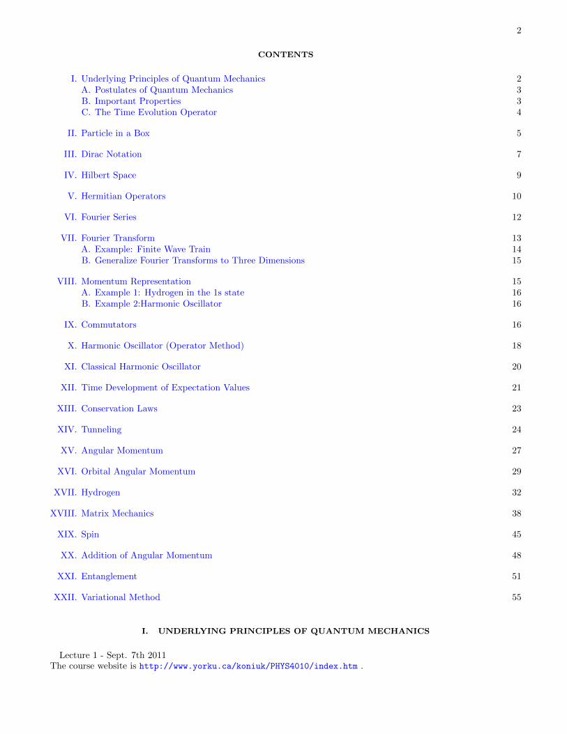
CONTENTS

I. Underlying Principles of Quantum Mechanics 2A. Postulates of Quantum Mechanics 3B. Important Properties 3C. The Time Evolution Operator 4

II. Particle in a Box 5

III. Dirac Notation 7

IV. Hilbert Space 9

V. Hermitian Operators 10

VI. Fourier Series 12

VII. Fourier Transform 13A. Example: Finite Wave Train 14B. Generalize Fourier Transforms to Three Dimensions 15

VIII. Momentum Representation 15A. Example 1: Hydrogen in the 1s state 16B. Example 2:Harmonic Oscillator 16

IX. Commutators 16

X. Harmonic Oscillator (Operator Method) 18

XI. Classical Harmonic Oscillator 20

XII. Time Development of Expectation Values 21

XIII. Conservation Laws 23

XIV. Tunneling 24

XV. Angular Momentum 27

XVI. Orbital Angular Momentum 29

XVII. Hydrogen 32

XVIII. Matrix Mechanics 38

XIX. Spin 45

XX. Addition of Angular Momentum 48

XXI. Entanglement 51

XXII. Variational Method 55

I. UNDERLYING PRINCIPLES OF QUANTUM MECHANICS

Lecture 1 - Sept. 7th 2011The course website is http://www.yorku.ca/koniuk/PHYS4010/index.htm .

3

A. Postulates of Quantum Mechanics

1. To every observable there corresponds an operator. For example to the observable A(e.g. energy,momentum,

position, etc.) there corresponds an operator A. Every measurement of A gives a value, a, s.t. a is an eigenvalue

of the operator A. i.e. for an eigenfunction of A, φ, Aφ = aφ.

2. Measurement of observable A yields the value a, and then leaves the state in the state φa. i.e.

Aφa = aφa

3. All possible information is contained in the wavefunction, Ψ(r, t).

4. Ψ developes in time according to the Schrodinger wave equation (SWE)

i~∂Ψ(r, t)

∂t= HΨ(r, t) (I.1)

B. Important Properties

The average value (expectation value) of an observable C at time t is given by

〈C〉 (t) =

∫Ψ∗(r, t)CΨ(r, t)dr (I.2)

Experimentally this would be done by preparing an ensemble of identical initial states Ψ(r, 0) and measure C at timet. This will generate a set of values, c1, c2, c3, ..., cN (where N is the number of measurements)

〈C〉 =1

N

N∑i=1

ci (I.3)

We can also interpret this as

〈C〉 =∑i

ciP (ci) (I.4)

The uncertainty (or standard deviation) in c is given by ∆c:

∆c =

√〈c2〉 − 〈c〉2 (I.5)

The modulus of Ψ is given by

Ψ∗(r, t)Ψ(r, t) = |Ψ(r, t)|2 (I.6)

|Ψ|2dx =

probability to findparticle at point x︷ ︸︸ ︷

P (x)dx (I.7)

The normalization condition is: ∫ ∞−∞

P (x)dx = 1 (I.8)

Lecture 2 - Sept. 9th 2011

4

C. The Time Evolution Operator

Suppose H doesn’t depend on time. (i.e. H = ˆH(r). Assume Ψ(r, t) = φ(r)T (t)) Plugging this result into theSWE:

i~∂(φT )

∂t= HφT (I.9)

i~φ∂T

∂t= THφ (I.10)

Divide both sides by ψ:

f︷ ︸︸ ︷i~

1

T

∂T

∂t=

g︷ ︸︸ ︷1

φHφ (I.11)

Thus f(t) = g(r) (regardless of t and r) The only way this can be true is if f(t) = g(r) = E where E is some constant.This generates two equations

i~∂T

∂t= ET (I.12)

and

Hφ = Eφ (I.13)

Notice that equation I.13 contains all the physics of the problem while the time equation contains no physics (doesnot contain the Hamiltonian). Equation I.12 can be solved by:

T (t) = e−iEt/~ (I.14)

Thus if the problem is seperable then the time dependance is always given by the above equation. All this term doesis changes the phase of the wavefunction (shifts the magnitude of the wavefunction from the real and complex partof the wavefunction). This time dependence is often referred to as trivial time dependence.

Equation I.13 is an eigenvalue problem. E is the eigenvalue and φ is the eigenfunction of the operator H. Thereare typically infinitely many solutions:

Hφn = Enφn (I.15)

With

Ψn(r, t) = φn(r)T (t) (I.16)

Ψn(r, t) = φn(r)e−iEnt/~ (I.17)

The probability density can depend on time if we don’t have an eigenfunction.The initial value problem: If we know the Ψ(r, 0) then we can determine Ψ for all time (i.e. Ψ(r, t))

i~∂Ψ

∂t= HΨ (I.18)

⇒ ∂Ψ

∂t=−i~HΨ (I.19)

⇒ ∂Ψ

∂t+ i

H

~ψ = 0 (I.20)

⇒ ∂

∂t

(exp(itHf/~)Ψ(r, t)

)= 0 (I.21)

Note: For this to be true we have to assume that H = H(r)Comments:

5

1. Notice that in the factor exp( itH~ ), H is an operator (could be a matrix). This can be understood by the realdefinition of the exponential function (a power series expansion):

exp(itH/~) = 1 +itH

~+

(itH)2

~22!+ ... (I.22)

This operator is defined as:

U−1 ≡ exp

(itH

~

)(I.23)

Lets carry on with our solution: ∫ t′

0

∂

∂t

(exp(itHf/~)Ψ(r, t)

)dt =

∫ t′

0

0dt (I.24)

By the fundamental theorem of calculus:

exp(it′Hf/~)Ψ(r, t′)− exp(0)Ψ(r, 0) = 0 (I.25)

You are free to change the dummy variable t′ to t and multiplying by U :

Ψ(r, t′) = exp(−it′Hf/~)Ψ(r, 0) (I.26)

The operator U is called the time evolution operator.Note that this is true for any state. Now suppose the initial state is an eigenstate (also called stationary states)

of H. Hence:

Ψ(r, 0) = φn(r) (I.27)

⇒ Ψ(r, t) = Uφn(r) (I.28)

= exp(−iHt/~)φn(r) (I.29)

= exp(−iEnt/~)φn(r) (I.30)

Hence in this special case the time ordering operator is just the trivial phase found earlier.

Lecture 3

II. PARTICLE IN A BOX

Step 1:Write down the potential

V (x) =

V = 0 0 < x < a

V (x) =∞ x ≤ 0, x ≥ a(II.1)

Step 2:Write down the S.E.

− ~2

2m

∂2

∂x2Ψ + V (x)Ψ = i~

∂Ψ

∂t(II.2)

The time portion is given by (assuming a separable solution)

T (t) = exp(−iEt/~) (II.3)

6

Thus the time independent problem is now given by

− ~2

2m

∂2

∂x2φ(x) + V (x)φ(x) = Eφ(x) (II.4)

Step 3:Outside the box the solution is trivial. It is zero.Inside the box the equation is given by

∂2

∂x2φ(x) = −k2φ(x) (II.5)

Where k is given by

k2 =2mE

~2(II.6)

The solution is given by

φ(x) = A sin(kx) +B cos(kx) (II.7)

Step 4:Check the boundary conditions

φ(0) = 0 = B (II.8)

φ(a) = 0 = Asin(ka) (II.9)

(II.10)

Hence we have the trivial solution (no particle) unless

ka = nπ ( n is an integer) (II.11)√2mE

~2a = nπ (II.12)

⇒ En =(nπa

)2 ~2

2m(II.13)

Hence E developed an index and energy quantization came out. Note that k also has an index:

kn =nπ

aThe wave-number is also quantized (II.14)

φn(x) = A sin(nπx

a

)(II.15)

Note the energy levels rise rapidly they go as n2. Note we were dealing with a homogeneous differential equation andhence isn’t fixed yet. This can be done using the normalization condition:

(II.16)∫ ∞−∞|φn|2dx =

∫ a

0

A2 sin2(nπx

a

)dx (II.17)

A2 a

2= 1 (II.18)

Hence

A =

√2

a(II.19)

Notice that the normalization constant is independent of the particular quantum number n.Therefore

φn(x) =

√2

asin(nπx

a

), En =

n2~2π2

2ma2(II.20)

7

Since the energy increases with decreasing a it means that quantum mechanics opposes this motion. This can bethought of as a quantum mechanical pressure on the outside of the box.Note that n can equal any integer

n = 1, 2, ... ( Infinity many bound states) (II.21)

Note the dimensions of φ are 1/√L and the dimensions of the P (the probability density) is 1/L. The energy levels

FIG. 1. The Wavefunctions of the Square Well and Their Corresponding Probability Densities

as well as the corresponding wavefunctions are shown in figure 1. Typically there are as many quantum numbers asdimensions of the problem.

Def 1. In any problem as ~→ 0 we recover classical physics. Equivalently we can recover classical physics as E →∞.

In our problem as E becomes large we should recover the classical distribution. The classical distribution is givenby

P (x) =

1/a 0 < x < a

0 x ≤ 0, x ≥ a(II.22)

In the limit of large E, we have a highly oscillating function from 0 to 2/a. For any experiment that tries to measurehow likely it is we will get to any finite region it will be 1/a.Assignment: Demonstrate by direct substitution that the first 5 eigenfunctions of the 1d well are indeed eigenfunctionsof the potential. Plot the first 5 eigenfunctions as well as the first 5 probability distributions. Due date: Wednesday.

Lecture 4 (September 14th, 2011)Note: Assignment 2 is up.

III. DIRAC NOTATION

The Dirac notation is a more abstract notation then was used up till now though it is more powerful. There is acorresponding notation in geometry referred to as coordinate free notation. The idea is a vector has a meaning beforea coordinate system is assigned to it. Similarly in quantum mechanics we have states which are independent of aparticular representation.A state labeled by a quantum number α is denoted by a “ket”. The symbol for the ket of α

|α〉 (III.1)

In the spatial representation the state |α〉 is given by Ψα(x). For example

〈α|β〉 =

∫ ∞−∞

ψ∗β(x)ψa(x)dx (III.2)

8

Note that this is analogous to

A ·B (III.3)

The analogy is even more evident by writing the integral as

lim∆xi→0N→∞

N∑i=1

ψ∗β(xi)ψα(xi)∆x (III.4)

Thus the wavefunctions are infinite dimension vectors. In coordinate free notation equation III.2 is given by

〈β|α〉 (III.5)

The “thing you dot kets with” is called a bra:

〈β| (III.6)

Bras and kets obey the following rules (a is some constant)

〈β|aα〉 = a 〈β|α〉 (III.7)

〈aβ|α〉 = a∗ 〈β|α〉 (III.8)

〈β|α〉∗ = 〈α|β〉 (III.9)

〈α|+ 〈β| = 〈α+ β| (III.10)

The state |x′〉 is an eigenstate of the position operator x.

x |x′〉 =

eigenvalue︷︸︸︷x′ |x′〉 (III.11)

〈x′|x〉 = δ(x′ − x) The Dirac Delta Function (III.12)

This makes sense since this expression reads what is the amplitude that a state |x′〉 coincides with the state |x|. Thesetwo states are distinctly different unless x = x′. The overlap of a position with the state α is

〈x′|α〉 = ψα(x′) (III.13)

This expression can be read as what is the amplitude that a state α is at x. Suppose you have a complete set of stateslabeled by integers (an orthonormal set): ∑

n

|n〉 〈n| = I (III.14)

To see that this is truly the identity:

I |m〉 =∑n

|n〉 〈n|m〉 (III.15)

=∑n

|n〉 δnm (III.16)

= |m〉 (III.17)

Lecture 5: September 16, 2011Notes for the assignment:

〈x〉 =

∫P (x, t)xdx (III.18)

P (x, t) = Ψ∗(x, t)Ψ(x, t) (III.19)

9

Ψ(x, t) =1√2

(φ1(x)e−iω1t + φ2(x)e−iω2t

)(III.20)

E1 = ~ω1 =~2π2

2ma2(III.21)

Continuing with the lecture

〈x|α〉 = ψα(x) (III.22)

〈β|x〉 = ψβ(x)∗ (III.23)

|α〉 = ket, ”vector” (III.24)

〈β| = bra, ”dual vector” (III.25)

Dual vectors are the objects that come from the scalar product with kets.

〈α|β〉 =

∫ψ∗α(x)ψβ(x)dx (III.26)

Aside (Cultural):The place where these are completely different objects are in differential geometry (general relativity).The objects dual to vectors are called one-forms. Maxwell’s equals can be written in differential geometry languageas:

dF = 0 (III.27)

d ∗ F = J (III.28)

IV. HILBERT SPACE

Recall Cartesian 3-space. We have vectors:

v = (vx, vy, vz) (IV.1)

v = exvx + eyvy + ezvz (IV.2)

We say that (ex, ey, ez) form a basis that spans the vector space. In other words we can build any vector in the vectorspace by a linear combination of the basis vectors.Inner Product:

v · u = vxux + vyuy + vzuz (IV.3)

Length:√v · u = |v| (IV.4)

1. The Hilbert space(H) is analogous to this space.The space is linear

For a constant ”a” aφ is also in the Hilbert space

If ψ and φ are in H then so is ψ + φ.

2. There is an inner product

〈α|β〉 =

∫ψ∗α(x)ψβ(x)dx (IV.5)

3. Any element of H has a ”length”

〈α|α〉 = ||α||2 (IV.6)

4. H is complete: Every Cauchy sequence of functions (or states) in H converges to an element in H.i.e. H contains the limit points)To understand this definition we need to define the Cauchy sequence:

10

Def 2. Cauchy Sequence: A sequence that as we go on in the sequence the difference gets smaller and smallerbetween neighboring number.

Mathematically, given the sequence xi any ε for some i:

|xi+1 − xi| ≤ ε (IV.7)

A Cauchy sequence can converge to a number that is not rational (the limit point can be outside the set). Wesay the irrationals complete the rationals.

Lecture 6: September 19, 2011A quick summary of the different notations is given bellow

3-D Representation Bro-ket

v · v = 0∫ψ∗α(x)ψβ(x)dx = 0 〈α|β〉 = 0

(e1, e2, e3) (ψ1, ψ2, ..., ) (|1〉 , |2〉 , |3〉 , ...)v =

∑i aiei φ(x) =

∑n anφn(x) |α〉 =

∑n an |n〉

ei · ej = δi,j∫φ∗n(x)φm(x)dx = δn,m 〈n|m〉 = δn,m

en · v = an∫φ∗n(x)ψα(x)dx = an 〈n|α〉 = an

|α〉 =∑m

am |m〉 (IV.8)

〈n|α〉 =∑m

〈n |am|m〉 (IV.9)

=∑m

am 〈n|m〉 (IV.10)

=∑m

amδn,m (IV.11)

= an (IV.12)

Word of warning: Sometimes we choose basis sets in H that are labeled by a continuous valued label. An example ofthis is the wave number: |k〉. This can be used as:

〈x|k〉 = eikx (IV.13)⟨k|∫x

|x| 〈x| k⟩dx =

∫ ∞−∞

(1)dx =∞ (IV.14)

The reason the overlap is infinity is because the plane waves are non-normalizable.

V. HERMITIAN OPERATORS

Consider the operator A such that A |α〉 is also in H and⟨β|A|α

⟩. If there is another operator designated by A†

such that ⟨A†β|α

⟩=⟨β|Aα

⟩(V.1)

Then we say that A† is the Hermitian adjoint of A (It does not mean that A is hermitian).

Simplest possible operator A = a (where a is some number)⟨a†β|α

⟩= 〈β|aα〉 = a 〈β|α〉 = 〈a∗β|α〉 (V.2)

Hence a† = a∗. i.e. the hermitian adjoint of a complex number is its complex conjugate.Consider the operator D = ∂

∂x . ⟨β|Dα

⟩=

∫ ∞−∞

dxψ∗β(x)∂

∂xψα(x) (V.3)

11

By integration by parts:

=

:

0ψ∗β(x)ψβ(x)

∣∣∣∣∞−∞−∫ ∞−∞

dx

(∂

∂xψ∗β(x)

)ψα(x) (V.4)

The surface terms cancel due to normalization condition. Hence

D† = −D (V.5)

In the special case where

A† = A (V.6)

we say the operators are Hermitian.

Lecture 7 - Sept 21, 20111 Recall ∂∂x is not Hermitian, but

(∂∂x

)†= − ∂

∂x .Consider

A |n〉 = an |n〉 (V.7)

Then ⟨n∣∣∣A∣∣∣n⟩ = 〈n |an|n〉 (V.8)

= an 〈n|n〉 (V.9)

(V.10)

But if A is Hermitian then ⟨An|n

⟩= 〈ann|n〉 (V.11)

= a∗n 〈n|n〉 (V.12)

Hence an = a∗n (an is real). Consider now ⟨m∣∣∣A∣∣∣n⟩ = 〈m |an|n〉 (V.13)

= an 〈m|n〉 (V.14)

But ⟨m∣∣∣A∣∣∣n⟩ =

⟨A†m|n

⟩(V.15)

=⟨Am|n

⟩(V.16)

= 〈amm|n〉 (V.17)

= a∗m 〈m|n〉 = am 〈m|n〉 (V.18)

Therefore

(an − am) 〈m|n〉 = 0 (V.19)

If an 6= am then

〈m|n〉 (V.20)

Therefore eigenstate of Hermitian operators are orthogonal.

12

VI. FOURIER SERIES

Suppose f(x) is periodic with period 2. i.e. For some a and all n:

f(x+ na) = f(x) (VI.1)

Then we can write

f(x) =

a02 +

∑∞n=1 an cos(nx) for odd f∑∞

n=1 bn sin(nπx) for odd f(VI.2)

Where for all n:

an =

∫ 2

0

f(t) cos(nπt)dt bn =

∫ 2

0

f(t) sin(nπt)dt (VI.3)

Exercise: Prove that any function can be written as a Fourier expansionFor any interval -L to L for a general periodic function:

f(x) =a0

2+

∞∑n=1

(an cos

(nπxL

)+ bn sin

(nπxL

))(VI.4)

Where

an =1

L

∫ L

−Lf(t) cos

(nπt

L

)dt (VI.5)

bn =1

L

∫ L

−Lf(t) sin

(nπt

L

)dt (VI.6)

For an example consider the square wave:

f(x) =

0 − π < x < 0

1 0 < x < π(VI.7)

a0 = 1 (VI.8)

an =1

π

∫ π

0

cos (nt) dt = 0 It is an odd function shifted upwards (VI.9)

bn =1

π

∫ π

0

sin (nt) dt (VI.10)

=1

π

(1

n− cosnπ

n

)(VI.11)

=1

nπ(1− (−1)n) (VI.12)

Therefore

bn =

2nπ odd n

0 even n(VI.13)

f(x) =1

2+

2

π

(sinx+

sin 3x

3+ ...

)(VI.14)

The orthogonality statement∫ 2π

0

sin (mx) sin (nx) = πδnm Unless m = n = 0 (VI.15)∫ 2π

0

cos (mx) cos (nx) = πδnm (VI.16)∫ 2π

0

sin (mx) cos (nx) = πδnm = 0 Unless m = n = 2π (VI.17)

13

VII. FOURIER TRANSFORM

Lecture 8 - September 23rd, 2011The Fourier series of a function f is given by

f(x) =a0

2+

∞∑n=1

an cos(nπxL

)+ bn sin

(nπxL

)(VII.1)

Where

an =1

L

∫ L

−Lf(t) cos

(nπt

l

)dt (VII.2)

bn =1

L

∫ L

−Lf(t) sin

(nπt

L

)dt (VII.3)

Explicitly:

f(x) =1

2Lf(t)dt+

1

Lcos(πnxL

)∫ L

−Lf(t) cos

(nπt

L

)dt+

1

L

∞∑n=

sin(nπxL

)∫ ∞−L

f(t) sin

(nπt

L

)dt (VII.4)

=1

2L

∫ L

−Lf(t)dt+

1

L

∞∑n=

∫ L

−Lf(t) cos

(nπL

(t− x))dt (VII.5)

Now let L→∞ (non-periodic function). Set

nπ

L= ω (VII.6)

This is equivalent to making the spacing between neighboring ω’s (∆ω = πL ) goes to 0. i.e. ω is continuous. In this

limit:

f(x) =1

π

∞∑n=1

∆ω

∫ ∞−∞

f(t) cos (ω (t− x)) dt (VII.7)

Notice the first integral went to zero due to the 1L dependence and no infinite summation over n. 1

π

∑∞n=1 ∆ω is just

the definition of an integral. Thus

f(x) =1

π

∫ ∞0

dω

∫ ∞−∞

f(t) cos (ω (t− x)) dt (VII.8)

Notice that in the integrand we have an even function of ω. Therefore we can divide by 2 and change the ω integralto:

f(x) =1

2π

∫ ∞−∞

dω

∫ ∞−∞

f(t) cos (ω (t− x)) dt (VII.9)

Now notice that the limits are symmetric so we can add an odd function of ω in the integrand (it will just go to zeroanyways)

f(x) =1

2π

∫ ∞−∞

dω

∫ ∞−∞

f(t) cos (ω (t− x)) + if(t) sin (ω (t− x)) dt (VII.10)

=1

2π

∫ ∞−∞

dω

∫ ∞−∞

f(t)e−iω(t−x)dt (VII.11)

=1

2π

F−1(x)︷ ︸︸ ︷∫ ∞−∞

eiωxdω

F(ω)︷ ︸︸ ︷∫ ∞−∞

f(t)e−iωtdt (VII.12)

Each of these F are transformations on the function f(t). Whatever the first one does, the second one undoes. F iscalled the Fourier transform of f(t). F−1(x) is the inverse Fourier transform of g(ω).

f(t)F−→ g(ω) f(t)

F−1

←−−− g(ω) (VII.13)

g(ω) is analogous to an.

14

Lecture 9 - Sept 30th, 2011Make up lecture Tuesday 2:30 pm.Recall:

f(x) =

∫ ∞−∞

f(t)

(1

2π

∫ ∞−∞

ei(t−x)ωdω

)dt (VII.14)

Definitions:

g(ω) =1√2π

∫ ∞−∞

f(t)e−iωtdt (VII.15)

We say that g(ω) is the Fourier transform of the function f (t). The function

f(t) =1√2π

∫ ∞−∞

g(ω)eiωtdω (VII.16)

is called the inverse Fourier transform.

A. Example: Finite Wave Train

f(t) =

sinω0t |t| < Nπ

ω0

0 |t| Nπω0

(VII.17)

The reason it is Nπω0

is because sinω0t→ sin(ωNπω0

)= 0. Note that this is an odd function. Remember that

eiωt = cosωt+ i sinωt (VII.18)

Since f(t) has a particular parity (i.e. is either odd or even) then only one cos or sin survive. The Fourier transformcan be split into two integrals:

gs(ω) =

√2

π

∫ ∞0

f(t) sinωtdt Fourier-Sin Transform (VII.19)

gc(ω) =

√2

π

∫ ∞0

f(t) cosωtdt Fourier-Cos Transform (VII.20)

Since we have an odd function we only have to do the sin integral:

gs(ω) =

√2

π

∫ Nπ/ω0

0

sinω0t sinωtdt (VII.21)

=

√2

π

∫ Nπ/ω0

0

1

2(cos (ω0 − ω) t− cos (ω + ω0)) dt (VII.22)

=1√2π

(sin ((ω0 − ω)Nπ/ω0)

ω0 − ω− sin ((ω0 + ω)Nπ/ω0)

ω0 + ω

)(VII.23)

Consider the case in which ω 1. Further lets focus on the region where ω ∼ ω0. This allows us to concentrate onthe first term.

gsω ∼1√2π

sin (ω0 − ω)Nπ/ω0

ω0 − ω(VII.24)

Taking the limit as ω0 → ω

limx→0

gs(ω) =1√2π

Nπ

ω0(VII.25)

15

At what values does gs(ω) vanish?

sin

((ω0 − ω)

Nπ

ω0

)= 0 (VII.26)

⇒ (ω0 − ω)Nπ

ω0= nπ (VII.27)

⇒ω0 − ω =nω0

N= ∆ω (VII.28)

Thus the distance between nodes (node spacing) is ω0/N . The width of the main peak is given by 2ω0/N . The

Lecture 10 - Oct 3rd, 2011Test 1: Nov 2ndTest 2: Nov. 21st

B. Generalize Fourier Transforms to Three Dimensions

Recall the 1d definition

g(k) =1√2π

∫ ∞−∞

f(x)e−ikxdx (VII.29)

The three dimensional analog is

g(k) =

(1√2π

)3 ∫ ∞−∞

∫ ∞−∞

∫ ∞−∞

f(x, y, z)e−ik·xdxdydz (VII.30)

VIII. MOMENTUM REPRESENTATION

〈x|α〉 = ψα(x) (VIII.1)

This is equal to probability amplitude to find a particle at position x for the state |α〉. Analogously,

〈p|α〉 = φα(p) (VIII.2)

is the probability amplitude to find a particle with momentum p for the state |α〉. The functions ψα(x) and φα(p)are Fourier transforms of one another

ψα(x)FT−−→ φα(p) (VIII.3)

The probability density in momentum (p) space is given by

Pα(p) = φ∗αφα(p) (VIII.4)

The dimensionless quantity that represents the probability of finding the particle with momentum between p andp+ dp is:

Pα(p)dp (VIII.5)

In three dimensions:

φα(p) =1

(2π~)3/2

∫ ∫ ∫ψα(r)ei(r·p)/~dr (VIII.6)

16

A. Example 1: Hydrogen in the 1s state

ψ1s(r) =

(1

πa30

)1/2

e−r/a0 (VIII.7)

Where a0 = ~2

me2 is the Bohr radius. Notice that the wave function is spherically symmetrical. Note if we want tofind the probability of finding the electron between radius r and r + dr is

ψ∗1s(r)ψ1s(r)r2dr (VIII.8)

The probability density is the greatest at the origin. However the radius of a spherical shell around the origin is sosmall that the probability to find an electron at that radius is zero. The most likely radius to find the electron is a0.However the most likely place to find the electron is the origin since that is where there are the highest density.The Fourier transform of this functions turns out to be (not proven)

φ1s(p) =23/2

π

a3/20 ~5/2

(a2op

2 + ~2)2 (VIII.9)

Notice the Fourier transforms are really different functions. The expectation value of position is given by

〈x〉 =

∫ ∞−∞

ψ∗(x)xψ(x)dx (VIII.10)

There are two ways to find the expectation value of momentum:

〈p〉 =

∫ ∞−∞

ψ∗(x)~i

∂

∂xψ(x)dx (VIII.11)

=

∫ ∞−∞

φ∗(p)pφ(p)dp (VIII.12)

B. Example 2:Harmonic Oscillator

The representations of the harmonic oscillator (ground?) state in position and momentum space are given by

ψ(x) ∝ e−(√mk/(2~))x2

(VIII.13)

φ(p) ∝ e−1

2~√

mkp2

(VIII.14)

Notice the functional forms are the same but one gets narrower as the other gets wider with α.

Lecture 11 - October 5th, 2011Makelectures delayed to October 25, and November 1st

IX. COMMUTATORS

[A, B

]= AB − BA (IX.1)

If[A, B

]= 0 we say the operators commute.

[x, p] =

[x,

~i

∂

∂x

](IX.2)

=~i

(x∂

∂x−(∂

∂x+

~ix∂

∂x

))= i~ (IX.3)

17

If[A, B

]= 0 then one can find simultaneous eigenfunctions of A and B. I.e.

Aψ = λψ (IX.4)

Bψ = λ′ψ (IX.5)

If[A, B

]6= 0 then one cannot find simultaneous eigenfunctions.

The expectation value of the distance from the average value is given by

∆2A ≡

⟨(A−

⟨A⟩)2

⟩(IX.6)

This value is referring the uncertainty. To avoid confusion lets expand this definition:⟨(A−

⟨A⟩)2

⟩=⟨A2 − 2A

⟨A⟩

+ A2⟩

(IX.7)

=⟨A2⟩− 2

⟨A⟩2

+⟨A2⟩

(IX.8)

=⟨A2⟩−⟨A⟩2

(IX.9)

Remember its implied that there is some state α at either end. i.e.

∆2A =

⟨α∣∣∣(A− ⟨A⟩)(A− ⟨A⟩)∣∣∣α⟩ (IX.10)

=⟨(A−

⟨A⟩)

α∣∣∣(A− ⟨A⟩)∣∣∣α⟩ (IX.11)

Call this term 〈f |f〉 where

|f〉 ≡(A−

⟨A⟩)|α〉 (IX.12)

likewise

∆2B = 〈g|g〉 (IX.13)

Where |g〉 =(B −

⟨B⟩)|α〉. But recall from mathematics the Schwarz inequality says:

〈f |f〉 〈g|g〉 ≥ |〈f |g〉|2 (IX.14)

Therefore

∆2A∆2

β = 〈f |f〉 〈g|g〉 ≥ |〈f |g〉|2 (IX.15)

remember that in general 〈f |g〉 is in general a complex number. Lets call this number z. Then

|z|2 = (<z)2+ (=z)2 ≥ (=z)2

=

(z − z∗

2i

)2

(IX.16)

Thus

∆2A∆2

B ≥(

1

2i[〈f |g〉 − 〈g|f〉]

)2

(IX.17)

Consider

〈f |g〉 =⟨(A−

⟨A⟩)(

B −⟨B⟩)⟩

(IX.18)

=⟨AB −

⟨A⟩B − A

⟨B⟩

+⟨A⟩⟨

B⟩⟩

(IX.19)

=⟨AB⟩−⟨A⟩⟨

B⟩

(IX.20)

18

〈g|f〉 =⟨BA⟩−⟨B⟩⟨

A⟩

(IX.21)

〈f |g〉 − 〈g|f〉 =⟨AB⟩−⟨BA⟩

(IX.22)

=⟨AB − BA

⟩(IX.23)

=⟨[A, B

]⟩(IX.24)

Hence

∆2A∆2

β ≥(

1

2i

⟨[A, B

]⟩)2

(IX.25)

Example:

[x, p] = i~ (IX.26)

For momentum and position then:

∆2x∆2

p ≥(i~2i

)2

(IX.27)

Equivalently:

∆2x∆2

p ≥~2

4(IX.28)

∆x∆p ≥~2

(IX.29)

When none commuting operators correspond to observables, we can them incompatible observables.

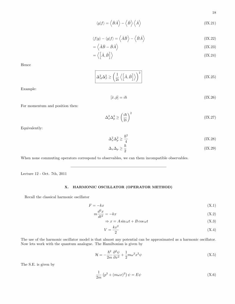
Lecture 12 - Oct. 7th, 2011

X. HARMONIC OSCILLATOR (OPERATOR METHOD)

Recall the classical harmonic oscillator

F = −kx (X.1)

md2x

dt2= −kx (X.2)

⇒ x = A sinωt+B cosωt (X.3)

V =kx2

2(X.4)

The use of the harmonic oscillator model is that almost any potential can be approximated as a harmonic oscillator.Now lets work with the quantum analogue. The Hamiltonian is given by

H = − ~2

2m

∂2ψ

∂x2+

1

2mω2x2ψ (X.5)

The S.E. is given by

1

2m

(p2 + (mωx)2

)ψ = Eψ (X.6)

19

The key idea is to factor the operator p2 + (mωx)2 . Consider if we were factoring two numbers u and v:

u2 + v2 = (iu+ v) (−iu+ v) (X.7)

Lets define

a− ≡1√

2~mω(ip+mωx) ; a+ ≡

1√2~mω

(−ip+mωx) (X.8)

Now if everything commuted then we would have H = a−a+ . However this is not the case as shown below:

a−a+ =1

2~mω(ip+mωx) (−ip+mωx) (X.9)

=1

2~mω(p2 +m2ω2x2 + imω (px− xp)

)(X.10)

=1

2~mω(p2 +m2ω2x2 − imωi~

)(X.11)

=1

~ωH+

1

2(X.12)

In the future we require a+a− so we may as well calculate it here:

a+a− =1

2~mω(−ip+mωx) (ip+mωx) (X.13)

=1

2~mω(p2 +m2ω2x2 − imω (px− xp)

)(X.14)

=1

~ω

(H− 1

2iω (i~)

)(X.15)

=

(1

~ωH− 1

2

)(X.16)

Rearranging gives

H = ~ω(a+a− +

1

2

)(X.17)

The commutator of a+, a− is

[a+, a−] =

(1

~ωH− 1

2

)−(

1

~ωH+

1

2

)(X.18)

= −1 (X.19)

Hence

Hψ = Eψ (X.20)

~ω(a+a− +

1

2

)ψ = Eψ (X.21)

Now suppose that we take

H (a+ψn) =

(a+a− +

1

2

)a+ψn (X.22)

= ~ωa+

(1

~ωH+ 1

)ψn (X.23)

= ~ωa+

(En~ω

+ 1

)ψn (X.24)

= (E + ~ω) a+ψn (X.25)

20

Hence the energy of the state acted on or “raised” by a+ is increased by a factor of ~ω.Now if we apply a− continuously to some state ψ then at one point you will get the state with no particle there at all(zero)

a−ψo = 0 (X.26)

Hence

1√2~mω

(ip+mωx)ψ0 = 0 (X.27)

~∂ψ

∂x+mωxψ = 0 (X.28)

∂ψ

∂x= −mω

~xψ (X.29)

ψ = e−mω2~ x2

(X.30)

XI. CLASSICAL HARMONIC OSCILLATOR

F = ma (XI.1)

−kx = ma (XI.2)

md2x

dt2+ kx = 0 (XI.3)

d2x

dt2+ ω2

ox = 0 (XI.4)

x(t) = A cosωot (XI.5)

E(t) =1

2mx2(t) +

1

2kx2(t) (XI.6)

Plugging the solution into the energy gives

E(t) =1

2mA2ω2

o sin2 ωot+1

2kA2 cos2 ωot (XI.7)

=1

2kA2 (XI.8)

Alternatively we can write

1

2mx2 +

1

2kx2 =

1

2kA2 (XI.9)

x = ωo√A2 − x2 (XI.10)

The probability to be between x and dx is

P (x)dx =dt

T/2(XI.11)

21

Where T is the period of oscillation. The period is given by T = 2πωo

. Thus:

P (x)dx =dt

T/2(XI.12)

=2ωodt

2π(XI.13)

=2ωo2π

dx

x(XI.14)

=2ωo2π

dx

ωo√A2 − x2

(XI.15)

=dx

π√A2 − x2

(XI.16)

The probability of finding the particle everywhere should be 1. Hence:

=

∫ A

−AP (x)dx (XI.17)

=

∫ A

−A

1

π

dx√A2 − x2

= 1 (XI.18)

Let x = Ay, dx = Ady.

=

∫ A

−A

A

π

dy√A2 −A2y2

(XI.19)

=

∫ A

−A

1

π

dy√12 − y2

(XI.20)

= 1 (XI.21)

Note that the probability density is infinite at x = A, however its not a problem since the probability is finite (as itmust be since our probability density is normalized)

XII. TIME DEVELOPMENT OF EXPECTATION VALUES

Consider ⟨A⟩

(XII.1)

In the x-representation for example we integrate this over all positions x. Hence the expectation value isn’t a functionof x. In other words:

d⟨A⟩

dt=∂⟨A⟩

∂t(XII.2)

∂⟨A⟩

∂t=

∂

∂t

∫ ∞−∞

ψ∗α(x)Aψα(x)dx (XII.3)

=

∫ ∞−∞

∂

∂t

(ψ∗α(x)Aψα

)dx (XII.4)

=

∫ ∞−∞

∂ψ∗α(x)

∂tAψα(x) + ψ∗α(x)

∂A

∂tψα(x) + ψ∗α(x)A

∂ψα(x)

∂tdx (XII.5)

Now the Schrodinger equation says that:

i~∂ψ

∂t= Hψ; −~∂ψ

∗

∂t= Hψ∗ (XII.6)

22

Thus ∫ ∞−∞

∂ψ∗Aψ

∂tdx =

∫ ∞−∞

i

~

(Hψ∗Aψ − ψ∗AHψ +

h

iψ∗∂A

∂tψ

)dx (XII.7)

Using representation free notation:

d⟨A⟩

dt=i

~

(⟨Hα|Aα

⟩−⟨α|AH|α

⟩+h

i

⟨α

∣∣∣∣∣∂A∂t∣∣∣∣∣α⟩)

(XII.8)

But the Hamiltonian is Hermitian. Hence

d 〈A〉dt

=i

~

⟨[H, A

]⟩+

⟨∂A

∂t

⟩(XII.9)

In most cases ∂A∂t = 0. In other words we’re mostly interested in operators that don’t have explicit time dependence.

In this case

d⟨A⟩

dt=i

~

⟨[H, A

]⟩(XII.10)

If[H, A

]= 0, then dA

dt = 0 . Therefore if A commutes with the Hamiltonian then⟨A⟩

is a constant of motion. As

an example consider the free case of V = 0. Then:[p, H

]= 0; H =

p2

2m(XII.11)

Hence momentum is conserved.Now consider the non free case:

H =p2

2m+ V (XII.12)

d 〈x〉dt

=i

~〈[H,x]〉 =

i

~

⟨[p2

2m+ V, x

]⟩(XII.13)

But V will certainly commute with x since V contains no derivatives but is just a function of x. Hence:

d 〈x〉dt

=i

~

⟨[p2

2m,x

]⟩(XII.14)

=i

2m~⟨[p2, x

]⟩(XII.15)

=i

2m~

⟨ppx− xpp

0︷ ︸︸ ︷−pxp+ pxp

⟩(XII.16)

=i

2m~〈p [p, x] + [p, x] p〉 (XII.17)

=i

2m~〈−i~p− i~p〉 (XII.18)

=i

2m~〈−i~p− i~p〉 (XII.19)

=〈p〉m

(XII.20)

This is an example of Ehrnfest’s principle which says that classical physics emerges as an average of quantum proba-bilities. Next consider [

H, p]

= [V, p] (XII.21)

= i~∂V

∂x(XII.22)

23

but

d 〈p〉dt

=i

~

⟨[H, p

]⟩(XII.23)

d 〈p〉dt

= −⟨∂V

∂x

⟩(XII.24)

This is Newton’s second law!

XIII. CONSERVATION LAWS

• In classical physics one can show that the invariance of physics under time translations leads to energy conser-vation.

• In a previous lecture we have derived the time evolution operator:

U = exp

(−iHt~

); U† = U−1 (XIII.1)

Consider the expectation value of a time evolved state α:

〈Uα |H|Uα〉 =⟨α∣∣U†HU ∣∣α⟩ (XIII.2)

Note that

U = exp (−iHt/~) = 1− iHt~

+

(−iHt~

)21

2+ ... (XIII.3)

Hence U commutes with H. Thus

〈Uα |H|Uα〉 = 〈α |H|α〉 (XIII.4)

So the expectation values of H is constant. In other words

d 〈E〉dt

= 0 (XIII.5)

This conservation of the energy. This can also be shown by the formula derived in the previous section for theexpectation value of an operator.

Consider any old function:

f (x+ ξ) = f(x) + f ′(x) (ξ) +1

2!f ′′(x)

(ξ2)

+ ... (XIII.6)

= exp

(ξ∂

∂x

)f(x) (XIII.7)

Consider the operator we just derived:

T ≡ exp

(ξ∂

∂x

)= exp

(i

~ξ~i

∂

∂x

)(XIII.8)

= exp

(i

~ξp

)(XIII.9)

Comparing with the time evolution operator we infer that this is the spatial translation operator. Alternatively bylooking at the definition you can see that when you let the operator act on some function f(x) and it brings you tothe function f(x+ ξ).

For the free Hamiltonian H = p2

2m , [T, H

]= 0 (XIII.10)

24

Therefore ⟨dp

dt

⟩= 0 (XIII.11)

Thus invariance under spatial transformation gives us momentum conservation.Now consider rotations:

f(φ) = f(φ+ ∆φ) (XIII.12)

= exp

(i

~∆φ

~i

∂

∂φ

)f(φ) (XIII.13)

= exp

(i

~∆φLz

)(XIII.14)

Define this operator as

R(∆φ) = exp

(i

~∆φLz

)(XIII.15)

This operator rotates the function by an amount ∆φ. If the rotation operator commutes with the Hamiltonian thenangular momentum will be conserved. i.e.

[Lz, H] = 0⇒ d 〈Lz〉dt

= 0 (XIII.16)

Next consider the parity operator (P).

Pf(x) = f(−x) (XIII.17)

If f(x) = f(−x) then we say f(x) even. If f(x) = −f(−x) then we say that f(x) is odd. For even f the eigenvalue ofP is 1 if f is odd then the eigenvalue of P is −1. If

[P, H] = 0⇒ d 〈P〉dt

= 0 (XIII.18)

Weak interactions violate parity conservation.

Lecture 15: October 21st, 2011

XIV. TUNNELING

Test 1: November 1Make up lecture is in room HNE on Nov. 1st, Nov 8thConsider the potential

V =

x < −a V = 0

−a < x < a V = Vo

x > a V = 0

(XIV.1)

Consider particles coming from the left

−~2

2m

d2ψ

dx2+ V ψ = Eψ (XIV.2)

For x < a:

−~2

2m

d2ψ

dx2= Eψ (XIV.3)

25

ψ =

Particles from left︷ ︸︸ ︷Aeik1x +

Particles from right︷ ︸︸ ︷Be−ik1x ; E =

~2k21

2m(XIV.4)

We keep both terms because particles may reflect back off the barrier.In the region −a < x < a:

−~2

2m

d2ψ

dx2+ Voψ = Eψ (XIV.5)

Bring the potential to the other side we have the same equation we have before with a new k:

ψ =

Particles from left︷ ︸︸ ︷Ceik2x +

Particles from right︷ ︸︸ ︷De−ik2x (XIV.6)

Where k2 = 2m~2 (E − Vo).

In x > a:

−~2

2m

d2ψ

dx2ψ = Eψ (XIV.7)

ψ =

Particles from left︷ ︸︸ ︷Geik1x +

Particles from right︷ ︸︸ ︷Ge−ik1x ; E =

~2k21

2m(XIV.8)

But here we can’t have any left movers, thus

ψ =

Particles from left︷ ︸︸ ︷Feik1x ; E =

~2k21

2m(XIV.9)

In this situation we can choose the energy E and |A|2. E corresponds to the energy of the particles and |A|2 correspondsto how many particles per second are incoming. B,C,D, and F are output that we get from the boundary conditions.We require continuity of the wavefunction as well as first derivative in order to have continuity of the second derivative(for S.E.).The boundary conditions are (where the points where the S.E. was solved now correspond to the labels, I,II, and III):

ψI(−a) = ψII(−a) (XIV.10)

ψ′I(−a) = ψ′II(−a) (XIV.11)

ψII(a) = ψIII(a) (XIV.12)

ψ′II(a) = ψ′III(a) (XIV.13)

All we really care to know is the transmission and reflection coefficients so we may as well set A = 1. If A = 1 thenwe know that

1 = |B|2 + |F |2 (XIV.14)

The boundary conditions tell us that

e−ik1a +Beika = Ce−k2a +Deik2a (XIV.15)

ik1

(e−k1a −Beik1a

)= ik2

(Ce−k2a −Deik2a

)(XIV.16)

Ceik2a +De−ik2a = Feik1a (XIV.17)

ik2

(Ceik2a +De−ik2a

)= ik1Fe

ik1a (XIV.18)

These equations can be solved using Mathematica. Switching to dimensionless variables: Define y = E/Vo and

η = 8ma2Vo

~2 the transmission coefficient comes out to

T =1

sinh2(√

1−y)4(1−y)y + 1

(XIV.19)

The points where the transmission is one are called transmission resonances. The transmission function in differentregimes is shown in figure 2.

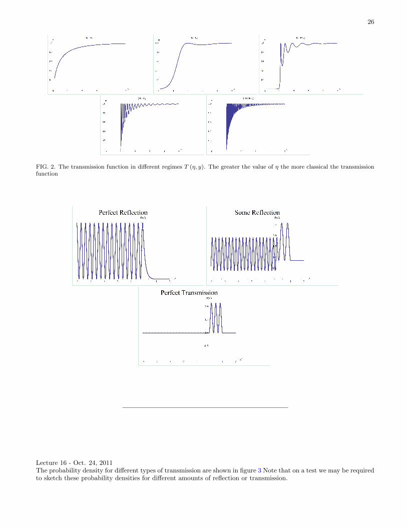
26

FIG. 2. The transmission function in different regimes T (η, y). The greater the value of η the more classical the transmissionfunction

Lecture 16 - Oct. 24, 2011The probability density for different types of transmission are shown in figure 3 Note that on a test we may be requiredto sketch these probability densities for different amounts of reflection or transmission.

27

XV. ANGULAR MOMENTUM

Classically:

L = r× p (XV.1)

= det

x y z

x y z

px py pz

(XV.2)

= x (ypz − ypy) + y (zpx − xpz) + z (xpy − ypx) (XV.3)

(XV.4)

Quantumly:

Lx = yh

i

∂

∂z− z ~

i

∂

∂y(XV.5)

The 3d operator angular momentum operator can be written

L =~ir×∇ (XV.6)

In order to find the following commutator makes use the the commutator:

[px, f(x)] = (pxf(x)) + fpx − fpx (XV.7)

= pxf(x) (XV.8)

[Lx, Ly] = LxLy − LyLx (XV.9)

= (ypz − zpy) (zpx − xpz)− (zpx − xpz) (ypz − zpy) (XV.10)

=~iypx −

~ixpy (XV.11)

=~i

(−Lz) (XV.12)

= i~Lz (XV.13)

Exercise: Do this . The commutators can be summarized by the following

[Li, Lj ] = i~εijkLk (XV.14)

Where the symbol εijk is called the Levi-Cevita and is defined as

εijk ≡

1 ijk cyclic

−1 ijk anti-cyclic

0 otherwise

(XV.15)

Lecture 17 - October 26th, 2011

L2 = L2x + L2

y + L2z (XV.16)

Using this it is straightforward to show that [Lx, L

2]

= 0 (XV.17)[Ly, L

2]

= 0 (XV.18)[Lz, L

2]

= 0 (XV.19)

28

We can pick a component (typically we pick Lz) and find simultaneous eigenfunctions of Lz, L2.

Note on notation: L is used for orbital angular momentum while S is used for spin angular momentum (intrinsic). Jis used for total angular momentum e.g. L + S, L1 + L2. No matter what the type of angular momentum we aredealing with is, L, J, or S the commutation relations are identical. e.g.

[Jx, Jy] = ~Jz (XV.20)

Define the ladder operators as:

J+ = Jx + iJy (XV.21)

J− = Jx − iJy = J†+ (XV.22)

List of commutation relations:

[Jz, J+] = ~J+ (XV.23)

[Jz, J−] = −~J− (XV.24)[J2, J+

]= 0 (XV.25)[

J2, J−]

= 0 (XV.26)

Further we can show that

J2 = J∓J± + J2z ± ~Jz (XV.27)

[J+, J−] = 2~Jz (XV.28)

Let

Jz |m〉 = m~ |m〉 (XV.29)

Consider

Jz (J+φm) = (~J+ + J+Jz)φm (XV.30)

= ~J+ + J+m~φm (XV.31)

= J+ (m+ 1) ~J+φm (XV.32)

Thus the state J+φm is an eigenfunction of Jz with the eigenvalue ~ (m+ 1). Thus J+ is called a raising or ladderoperator.

J+φm ∝ φm+1 (XV.33)

J−φm ∝ φm−1 (XV.34)

Now [J2, Jz

]= 0 (XV.35)

Therefore

J2φm = ~2K2φm (XV.36)

Where K is some value (not yet known). Consider

J+J2φm = J+~2K2φm (XV.37)

= ~2K2J+φm (XV.38)

∝ ~2K2φm+1 (XV.39)

J+φm has the same eigenvalue as J2. ⟨J2⟩

= ~K2 =⟨J2x

⟩+⟨J2y

⟩+⟨J2z

⟩(XV.40)

=⟨J2x

⟩+⟨J2y

⟩+ ~2m2 (XV.41)

(XV.42)

29

Now⟨J2x

⟩and

⟨J2y

⟩are positive definite quantities. The proof of this is shown below. Here |α〉 is some state in the

Jz basis and |α〉 is some state in the i basis, J ′i is the operator is the diagonalized basis and U is the matrix thatdiagonalizes Jx. ⟨

J2i

⟩= 〈α| J2

i |α〉 (XV.43)

= 〈α|U†UJiU†UJiU†U |α〉 (XV.44)

= 〈α′| J ′2i |α′〉 (XV.45)

= j2i (XV.46)

Where here ji is the eigenvalue of Ji. Thus⟨J2x

⟩and

⟨J2y

⟩are positive definite which means that

~2K2 ≥ ~2m2 (XV.47)

and hence

|K| ≥ |m| (XV.48)

This means that a given sequence of m’s must lie between |K| and − |K|. Therefore

J+ |mmax〉 = 0 (XV.49)

J− |mmin〉 = 0 (XV.50)

J2 |mmax〉 =(J2x + J2

y + J2z

)|mmax〉 (XV.51)

=

((J+ + J−

2

)2

+

(J+ − J−

2i

)2

+ J2z

)|mmax〉 (XV.52)

=1

4(J+J− + J−J+ + J+J− + J−J+) |mmax〉 (XV.53)

=1

2

((J+J− + J−J+ + 2J2

z

)|mmax〉

)(XV.54)

~2K2 |mmax〉 =(~Jz + J2

z

)|mmax〉 (XV.55)

Similarly

~2K2 = ~2mmin (mmin − 1) (XV.56)

Solving these equations says that

mmax = −mmin (XV.57)

or

mmin = mmax + 1 (XV.58)

We can throw out the second solution on physical grounds (we can’t have a maximum m be smaller then the minimumm).

Therefore if mmax = j (define j this way) then mmin = −j and therefore

m = (−j,−j + 1, ..., j − 1, j) (XV.59)

J2 |m〉 = ~2j (j + 1) |m〉 (XV.60)

XVI. ORBITAL ANGULAR MOMENTUM

Now lets specialize to eigenfunctions of orbital angular momentum.

L2φlm = ~2l (l + 1)φlm (XVI.1)

Lzφlm = m~φlm (XVI.2)

30

We want explicit constructions of φlm. Recall:

Lz =~i

(x∂

∂y− y ∂

∂x

)(XVI.3)

We could proceed in this way but its more natural to move to spherical coordinates. The coordinate system is shownin figure 3 Exercise: Transform Lz into spherical coordinates. This can be found by finding the transformation from

x

y

z

theta

phi

FIG. 3. The spherical coordinate system

x

y

z

→ r

θ

φ

(XVI.4)

and then taking the inverse of the transformation. This gives the following

∂

∂y= (sin θ sinφ)

∂

∂r+

(sin θ sinφ

r

)∂

∂θ+

(cos θ

r sin θ

)∂

∂φ(XVI.5)

∂

∂x= (sin θ cosφ)

∂

∂r+

(cos θ cosφ

r

)∂

∂θ−(

sinφ

r sin θ

)∂

∂φ(XVI.6)

By substitution (ideally blended with astute observations)

Lz =~i

(0∂

∂r+ 0

∂

∂θ+r sin θ cosφωφ

r sin θ+r sin θ sinφ sinφ

r sin θ

∂

∂θ

)(XVI.7)

=~i

∂

∂θ(XVI.8)

The other operators are not as compact

Ly = i~(− cosφ

∂

∂θ+ cotφ sinφ

∂

∂φ

)(XVI.9)

Lx = i~(

sinφ∂

∂θ+ cot θ cosφ

∂

∂φ

)(XVI.10)

L2 = L2x + J2

y + J2z (XVI.11)

= −~2

(1

sin θ

∂

∂θ

(sin θ

∂

∂θ

)+

1

sin2 θ

∂2

∂φ2

)(XVI.12)

31

L2φlm = ~2l (l + 1)φlm (XVI.13)

Lzφlm = m~φlm (XVI.14)

The solutions to the differential equation is

φlm (θ, φ) = Ylm (θ, φ) (XVI.15)

The spherical harmonics are properly normalized:∫|Ylm (θ, φ)|2 dΩ = 1 (XVI.16)

LzYlm (θ, φ) = m~Ylm (θ, φ) (XVI.17)

⇒ Ylm (θ, φ) ∝ eimφ (XVI.18)

Singlevaluedness of these solutions forces

eimφ = eimφ+im2π (XVI.19)

Hence

e2imπ = 1 (XVI.20)

In other words m ∈ Z. In order to keep the φ component normalized we require that the φ component is

1√2πeimφ (XVI.21)

Now subbing into the spherical harmonics says that

Ylm (θ, φ) =eimφΘ(θ)√

2π(XVI.22)

Plugging this into

L2Ylm = ~2l (l + 1)Ylm (XVI.23)

⇒ 1

sin θ

(d

dθ

(sin θ

dΘ(θ)

dθ

))+

(l(l + 1)− m2

sin2 θ

)Θ(θ) = 0 (XVI.24)

This is an ugly differential equation. Define

µ = cos θ (XVI.25)

Θ(θ)lm = Pml (µ) (XVI.26)

Where these are the associated Legendre Polynomials.

Pml (µ) = (−1)m(1− µ2

)m/2 dm

dµmPl(µ) (XVI.27)

Where Pl(µ) are the Legendre Polynomials defined as

Pl(µ) =1

2ll!

dl

dµl(µ2 − 1

)l(XVI.28)

The first few Legendre Polynomials are

Po(µ) = 1 (XVI.29)

P1(µ) = µ (XVI.30)

P2(µ) =1

8

d2

dµ2

(µ4 − 2µ2 + 1

)=

3µ2 − 1

2(XVI.31)

32

-1 1

P0

P1

P2

The first few Associated Legendre Polynomials are

P00(µ) = 1 = 1 (XVI.32)

P10(µ) = µ = cos θ (XVI.33)

P11(µ) = −√

1− µ2 = − sin θ (XVI.34)

Putting this all together we can write the spherical harmonics.

Ylm(θ, φ) (XVI.35)

with

L2Ylm = ~2l (l + 1)Ylm; LzYlm = m~ (XVI.36)

Ylm(θ, φ) =

(2l + 1

4π

(l −m)!

(l +m)!

)1/2

Plm (cos θ) eimφ (XVI.37)

The spherical harmonics are orthonormal:∫Y ∗lm (θ, φ)Yl′,m′ (θ, φ) dΩ = δm,m′δl,l′ (XVI.38)

Due to the phase we have

Yl,−m = (−1)mY ∗lm (XVI.39)

The first few are tabulated below

Y0,0 = 1√4π

Y1,1 = − 12

(3

2π

)1/2sin θeiφ

Y1,0 = 12

(3π

)1/2cos θ

Y1,−1 = 12

(3π

)1/2sin θe−iφ

In order to plot these we can plot |Ylm| and set |Ylm| = r. In other words the distance from the origin beginlarge implies that the function is large (note this is only for plotting purposes). Its important to note there is no φdependence. So the plot is independent of the angle in the x,y plane.

XVII. HYDROGEN

H = − ~2

2m∇2 − 1

4πεo

q2Z

r(XVII.1)

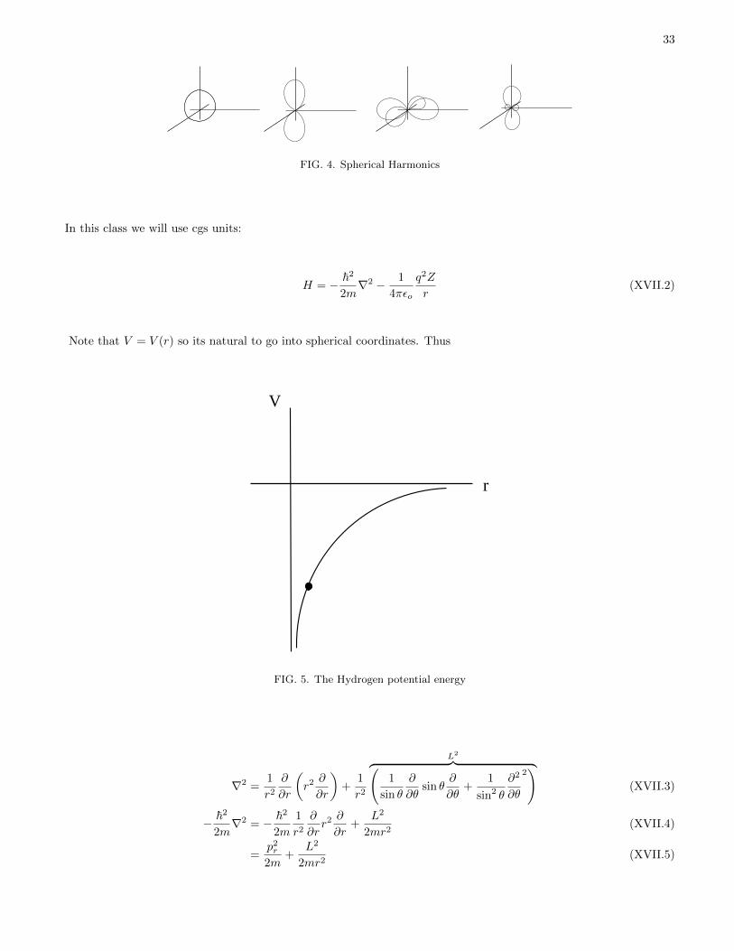
33

FIG. 4. Spherical Harmonics

In this class we will use cgs units:

H = − ~2

2m∇2 − 1

4πεo

q2Z

r(XVII.2)

Note that V = V (r) so its natural to go into spherical coordinates. Thus

V

r

FIG. 5. The Hydrogen potential energy

∇2 =1

r2

∂

∂r

(r2 ∂

∂r

)+

1

r2

L2︷ ︸︸ ︷(1

sin θ

∂

∂θsin θ

∂

∂θ+

1

sin2 θ

∂2

∂θ

2)

(XVII.3)

− ~2

2m∇2 = − ~2

2m

1

r2

∂

∂rr2 ∂

∂r+

L2

2mr2(XVII.4)

=p2r

2m+

L2

2mr2(XVII.5)

34

Theorem: The ground state of a system has the full symmetry of the problem.This lovely coincidence that L2 showed up was of course not actually a coincidence.

L2 = (r× p)2

(XVII.6)

= r2p2 − (r · p)2

(XVII.7)

r2p2 = (r · p)2

+ L2 (XVII.8)

p2

2m=

(r · p)2

r2+ L2r2 (XVII.9)

= (r · p)2

+L

2mr2(XVII.10)

=p2r

2m+

L2

2mr2(XVII.11)

Thus (p2r

2m+

L2

2mr2− Ze2

r

)ψ (r, θ, φ) = Eψ (r, θ, φ) (XVII.12)

Using the relation[L2, H

]= 0 (easy to see by looking at the Hamiltonian term by term), we know that they share

eigenfunctions. Hence

ψ (r, θ, φ) = R(r)Ylm (θ, φ) (XVII.13)

Note it is always the case that if V = V (r) then ψ = R(r)Ylm(θ, φ).

Lecture 18 - November 1st, 2011Recall (switched to MKS)(

− ~2

2m

1

r2

∂

∂r

(r2 ∂

∂r

)+

L2

2mr2− Ze2

4πεor

)ψ (r, θ, φ) = Eψ (r, θ, φ) (XVII.14)

Since we have a central potential (i.e. V = V (r)) we can write ψ(r) = R(r)Ylm (θ, φ)

[H,L2

]= 0⇒

Hψ = Eψ

L2ψ = ~2l (l + 1)ψ(XVII.15)

Plugging in ψ(r) = R(r)Ylm (θ, φ) into our equation.(− ~2

2m

1

r2

∂

∂r

(r2 ∂

∂r

)+l (l + 1)

2mr2− Ze2

4πεor

)R(r) = ER(r) (XVII.16)

Note we have reduced a 3D problem to 1D. Introduce a new function U(r) ≡ rR(r) to simplify the differentialequation. This gives (

− ~2

2m

d2

dr2+

~2l (l + 1)

2mr2− e2

4πεo

1

r

)U(r) = EU(r) (XVII.17)

The nice thing about this equation is that this looks just like 1D quantum mechanics in the variable r, but thepotential term is an effective potential given by

Veff (r) =~2l (l + 1)

2mr2− e2

4πεor(XVII.18)

Note that when l = 0 The potential is just the Coloumb potential. The effective potential is shown in figure 6 Whatis the natural scale for this problem? We can build the scale from the constants in the problem:

[m]α

[~]β

[e2

4πεo

]γ= L (XVII.19)

[M ]α

[ML2

T

]β [ML3

T 2

]γ= L (XVII.20)

35

Coloumb

Angular momentum

Centrifugal Barrier

FIG. 6. The Effective potential of Hydrogen

So we know that

α+ β + γ = 0 (XVII.21)

−β − 2γ = 0 (XVII.22)

2β + 2γ = 1 (XVII.23)

The solution of this set of equations is

α = −1 (XVII.24)

β = 2 (XVII.25)

γ = −1 (XVII.26)

Thus

[L] =4πεo~2

me2= 0.53× 10−10m ≡ ao (XVII.27)

Note that with little work we already know the natural scale for atomic systems (A).Its also convenient to introduce

κ ≡√−2mE

~; ρ ≡ κr; ρo =

2

aoκ(XVII.28)

With these changes we get

d2v

dρ2=

(1− ρo

ρ+l (l + 1)

ρ2

)v (XVII.29)

Consider ρ→∞.

d2v

dρ2= v (XVII.30)

⇒ u(ρ) = Ae−ρ +Beρ (XVII.31)

36

B must be zero due to normalization requirements. Now consider ρ→ 0:

d2v

dρ2=l (l + 1)

ρ2v (XVII.32)

u(ρ) = Cρl+1 +Dρ−l (XVII.33)

Where for normalization we require D = 0. Substitute u(ρ) = ρl+1e−lv(ρ) into the radial equation

ρd2v

dρ2+ 2 (l + 1− ρ)

dv

dρ+ (lo − 2 (l + 1)) v = 0 (XVII.34)

Frobenius method gives that the result is the associated Laguerre polynomials.

Lpq−p(x) ≡ (−1)p ( d

dx

)pLq(x)

Lq ≡ ex(ddx

)q(e−xxq)

L0 = 1

L1 = 1− xL2 = x2 − 4x+ 2

L00 = 1

L01 = −x+ 1

L02 = x2 − 4x+ 2

Reassemble our radial wavefunctions:

Rnl =1

rρl+1e−ρL2l+1

n−l−1(2π) (XVII.35)

Where κ = 1aon

, ρ = raon

. The energies are

En =E1

n2(XVII.36)

Where

E1 = −1

2mc2α2; α ≡ e2

4πεo~c≈ 1

137(XVII.37)

α is called the fine structure constant. It is a measure of the electromagnetic interaction.

November 7th, 2011The radial equation is (

− ~2

2m

1

r2

∂

∂r

(r2 ∂

∂r

)+ ~2 l (l + 1)

2mr2− e2

4πεo

1

r

)R(r) = ER(r) (XVII.38)

Notice that the only place were we have l dependence is in the middle term. Also notice that there is no m dependencein the Schrodinger equation. This reflects the fact that our problem is rotationally invariant. mmeasures the projectionof l into the z axis and our choice of z is arbitrary. We can break this rotational symmetry (by for example adding amagnetic field) in this case the energy would depend on m. Note there has been a change in notation (at least withhis online notes):

ρ ≡ 2κr; ao =4πεo~2

me2= 0.53A; κ =

√−2mE

~(XVII.39)

The new differential equation is

d2u

dρ2=

(1

4− n

ρ+l(l + 1)

ρ2

)(XVII.40)

37

Where n = 1aoκ

. The result is

u(ρ) = ρl+1e−ρ/2u(ρ) (XVII.41)

Using the Frobenius method we find that we don’t have well behaved solutions unless the series Frobenius seriesterminates. The ones that are finite are the Laguerre polynomials. They occur when n is an integer. Now we canfind the radial term:

Rnl(ρ) = ρle−ρ/2L2l+1n+l (ρ) (XVII.42)

Notice that the Rnl(ρ) depends on n and l and we call n the principle quantum number.

En = −1

2

mc2α2

n2; α ≡ e2

4πεo~c≈ 1

137(XVII.43)

Notice the eigenvalues don’t have any angular dependence! Thus two very different eigenfunctions

R20 =

(1

2ao

)3/2(2− r

ao

)e−r/2ao (XVII.44)

R21 =

(1

2ao

)3/21√3

(r

ao

)e−r/2ao (XVII.45)

have the same eigenvalues! This mysterious degeneracy in the eigenvalues is due to a hidden symmetry in the problem.

R10

R20

R21

FIG. 7. The Radial terms of the Hydrogen wavefunction

ψnlm(r) = Rnl(r)Ylm(φ, θ) (XVII.46)

∫ψ∗n′l′m′ψnlmr

2 sin θdrdθdφ = δn′nδl′lδm′m (XVII.47)

38

The radial probability distribution is

P (r) = r2R2nl(r) (XVII.48)

For the state 1s state:

P1,0(r) = r2R210(r) (XVII.49)

To find the maximum we take the derivative and set it to zero:

dP10

dr= 0 (XVII.50)

2re2rao − 2

aoe−2r/ao = 0 (XVII.51)(

r − r2

ao

)e−2r/ao = 0 (XVII.52)

This is zero at r = 0, r =∞, r = ao. It is a minima at ∞ and 0. It is a maximum at ao.

〈r〉 =

∫R10(r)rR10(r)r2dr (XVII.53)

=

∫ ∞0

P10rdr (XVII.54)

Where P10(r) is the radial probability distribution.

〈r〉 =

∫ ∞o

4

a3o

r2e−2r/aordr (XVII.55)

Define x = 2r/ao → dx = 2dr/ao

〈r〉 =

∫ ∞o

ao4x3e−xdx (XVII.56)

=ao4

3! (XVII.57)

=3ao2

(XVII.58)

Another interesting quantity is

〈r〉 = 〈x〉 x+ 〈y〉 y + 〈z〉 y (XVII.59)

= 0 (XVII.60)

This must be zero since we have reflection symmetry. This is true for all Hydrogen eigenstates (but not for the linearcombinations)

Lecture 19 - November 19th, 2011

XVIII. MATRIX MECHANICS

Consider some basis set

B1 = (φ1, φ2, ..., .φn) (XVIII.1)

We have already encountered some basis sets (√2

asin(nπy

a

))(XVIII.2)(

AnHn(ξ)e−ξ2/2)

(XVIII.3)

(Rnl(r)Ylm(φ, θ)) (XVIII.4)

39

Recall in Dirac notation

|α〉 =∑n

|n〉 〈n|α〉 (XVIII.5)

〈n|α〉 = an (XVIII.6)

|α〉 =∑n

an |n〉 (XVIII.7)

Knowing what basis B and all the an is equivalent to knowing |α〉.Consider an operator F (arbitrary). Let

F |α′〉 = |α〉 (XVIII.8)

Now lets construct 〈q|α〉. Where |q〉 is some basis state.

〈q|α〉 = |q |F |α′〉 (XVIII.9)

=∑n

〈q |F |n〉 〈n|α′〉 (XVIII.10)

aq =∑n

Fqna′n (XVIII.11)

Where we have defined

Fqn ≡ 〈q |F |n〉 (XVIII.12)

=

∫φ∗qFφndr (XVIII.13)

We call Fqn a matrix element.

aq =∑n

Fqna′n (XVIII.14)

a1

a2

...

=

F11 F12 ...

F21 F22 ......

......

a′1a′2...

(XVIII.15)

We also call Fqn the matrix representation of the operator F.Consider

G |n〉 = gn |n〉 (XVIII.16)

This is an eigenvalue equation.

G =

g1 0 0

0 g2 0

0 0. . .

(XVIII.17)

The eigenfunctions are just

|n〉 =

0...

0

1

0...

0

(XVIII.18)

Recall some matrix properties

40

1. Matrix multiplication:

(AB)nq =∑p

AnpBpq (XVIII.19)

2. Inverse:

A−1A = I (XVIII.20)

A−1 =1

detAAadj ; Aadj = ATcofactor; Acof = (−1)

i+jMij (XVIII.21)

3. Determinant:

det(A) =∑σ∈Sn

sgn(σ)

n∏i=1

Ai,σ(n) (XVIII.22)

Where σ is the particular permutation. Sn is the set of permutations. sgn(σ) = +1,−1 depending on if we havean even or odd permutation.

4. Symmetry: If

AT = A (XVIII.23)

Then A is symmetric. If

AT = −A (XVIII.24)

Then A is antisymmetric.

5. Trace:

Tr (A) =∑n

Ann (XVIII.25)

6. Hermitian Adjoint:

A† = A∗T (XVIII.26)

A†qn = A∗nq (XVIII.27)

For Hermitian operators:

A† = A (XVIII.28)

The proof of Hermitian operators corresponding to real numbers in terms of matrices is straightforward. It alsoshows that Hermitian operators correspond to Hermitian matrices. Exercise try this!

7. Unitary:

U† = U−1 (XVIII.29)

We have seen one unitary operator already. The time evolution

e−iHt/~ (XVIII.30)

The importance of unitary operators is that they maintain inner products.

〈β′|α′〉 = 〈Uβ|Uα〉 (XVIII.31)

=⟨β∣∣U†U ∣∣α⟩ (XVIII.32)

= 〈βα〉 (XVIII.33)

41

How operators transform?

F |α〉 = |β〉 (XVIII.34)

FU−1 |α′〉 = U−1 |β′〉 (XVIII.35)

UFU−1 |α′〉 = UU−1 |β′〉 (XVIII.36)

F ′ |α′〉 = |β′〉 (XVIII.37)

Hence

F ′ = UFU−1 (XVIII.38)

Lecture 22 - November 11, 2011Recall the harmonic oscillator

H = − ~2

2m

∂2

∂x2+

1

2mωoc

2 (XVIII.39)

B = e−ξ2/2 (AoHo(ξ), A1H1(ξ), ...) (XVIII.40)

Where ξ2 = β2x2, β2 = mωo

~ . Another way to denote the basis is

B = (|0〉 , |1〉 , |2〉 , ...) (XVIII.41)

The action of the Hamiltonian

H |n〉 =

(n+

1

2

)~ωo |n〉 (XVIII.42)

In this basis the Hamiltonian:

H =

12~ωo 0 ...

0 32~ωo 0

... 0. . .

(XVIII.43)

Since we are in the eigenbasis We see that H is diagonal. Now consider

xmn = 〈m|x |n| (XVIII.44)

We can evaluate these matrix elements:

xmn =

∫AmHm(ξ)xAnHn(ξ)dx (XVIII.45)

However alternatively we can be clever and use ladder operators.

a+ =1√

2~mω(−ip+mωx) (XVIII.46)

a− =1√

2~mω(ip+mωx) (XVIII.47)

a+ |n〉 = (n+ 1)1/2 |n+ 1〉 (XVIII.48)

a− |n〉 =(n1/2

)|n− 1〉 (XVIII.49)

42

We can write the x operator as

x =1√2

1

β(a− + a+) (XVIII.50)

What is the a+ matrix?

(a+)mn = 〈m| a+ |n〉 (XVIII.51)

= 〈m| (n+ 1)1/2 |n〉 (XVIII.52)

= (n+ 1)1/2 〈m|n+ 1〉 (XVIII.53)

= (n+ 1)1/2

δm,n+1 (XVIII.54)

(a−)mn = n1/2δm,n−1 (XVIII.55)

Now we can construct the x

x =1√2

1

β

0 1 0 0 ...

1 0√

2 0 0

0√

2 0√

3 0

0 0√

3. . .

. . ....

......

. . .. . .

(XVIII.56)

This is a tridiagonal matrix.For bonus marks: Find the eigenvectors of this matrix numerically using Mathematica.What is a+a−

a+a− =

0 0 0 ...

0 1 0 ...

0 0 2. . .

......

. . .. . .

(XVIII.57)

This is simply the number operator. Thus we can write

H = ~ωo(N +

1

2

)(XVIII.58)

Angular momentum: [L2, Lz

]= 0 (XVIII.59)

L2 |lm〉 = ~2l (l + 1) |lm〉 (XVIII.60)

Lz |lm〉 = m~ |lm〉 (XVIII.61)

L2 = ~2

0 0 0 0 0 0

0 2 0 0 0 0

0 0 2 0 0 0

0 0 0 2 0 0

0 0 0 0 6 0

0 0 0 0 0. . .

(XVIII.62)

43

Lz = ~2

0 0 0 0 0 0

0 1 0 0 0 0

0 0 0 0 0 0

0 0 0 −1 0 0

0 0 0 0 2 0

0 0 0 0 0. . .

(XVIII.63)

L+ = Lx + iLy (XVIII.64)

L− = Lx − iLy (XVIII.65)

L± |l,m〉 = ((l ∓m) (l ±m+ 1))1/2 |l,m± 1〉 (XVIII.66)

〈l,m|L± |l′m′〉 = (l′ ∓m′) (l′ ±m′ + 1)1/2 ~δll′δn,m′±1 (XVIII.67)

Let’s look at the l = 1 subspace:

L2 = ~2

2 0 0

0 2 0

0 0 2

(XVIII.68)

Lx =~√2

0 1 0

1 0 1

0 1 0

(XVIII.69)

Lx =~√2

−i 0

i 0 −i0 i 0

(XVIII.70)

Lz = ~

1 0 0

0 0 0

0 0 −1

(XVIII.71)

The eigenvectors of Lz are

|l = 1,m = 1〉 =

1

0

0

; |l = 1,m = 0〉 =

0

1

0

; |l = 1,m = −1〉 =

0

0

1

(XVIII.72)

Lecture 23 - November 14th, 2011On the test:

• Tunneling

• Angular momentum

• Hydrogen

44

The eigenvalues of L2 are 2~2 (the same for all m). To diagonalize Lx is to

Lxv = λv (XVIII.73)

(Lx − λ) v = 0 (XVIII.74)

One solution is the trivial solution v = 0, but this isn’t interesting. To get interesting solutions:

det (Lx − λ) (XVIII.75)

det

−λ ~√

20

~√2−λ ~√

2

0 ~√2−λ

= 0− λ(λ2 − ~2/2

)+ λ~2/2 = 0 (XVIII.76)

This gives eigenvalues are 0,±~. To get eigenvectors plug λ’s back in. Plugging in λ = ~:−~ ~√

20

~√2−~ ~√

2

0 ~√2−~

v1

v2

v3

= 0 (XVIII.77)

~

−1 1√

20

1√2−1 1√

2

0 1√2−1

v1

v2

v3

= 0 (XVIII.78)

Solving the systems gives the following eigenvalues:

λ = ~1

2→

1√2

1

(XVIII.79)

λ = 0→ 1√2

1

0

−1

(XVIII.80)

λ = −~→ 1

2

1

−√

2

1

(XVIII.81)

The transformation is a Unitary Matrix (as expected):

U =1

2

1√

2 1√2 0 −

√2

1 −√

2 1

(XVIII.82)

In order to diagonalize Lx:

ULxU−1 =

1

2

1√

2 1√2 0 −

√2

1 −√

2 1

~√2

0 1 0

1 0 1

0 1 0

1

2

1√

2 1√2 0 −

√2

1 −√

2 1

(XVIII.83)

= ~

1 0 0

0 0 0

0 0 −1

(XVIII.84)

45

In terms of spherical harmonics what are the eigenvectors? Thus the eigenvector for λ = ~:

1

2

1√2

1

→ 1

2=(Y1,1(φ, θ) +

√2Y1,0(φ, θ) + Y1,−1(φ, θ)

)(XVIII.85)

=1

4

√3

2π

(sin θe−iφ + 2 cos θ + sin θeiφ

)(XVIII.86)

=1

2

√3

2π(cos θ +−i sin θ sinφ) (XVIII.87)

P (φ, θ) =1

4

3

2π

(cos2 θ + sin2 θ sin2 φ

)sin θ (XVIII.88)

∫P (φ, θ)dθdφ = 1 (XVIII.89)

Notice that since these aren’t eigenfunctions of z we know longer have rotational symmetry of φ! Now we can check

whether this truly is an eigenfunction of Lx = i~(

sinφ ∂∂θ + cos θ cosφ ∂

∂φ

). Notice that finding the eigenfunction of

this operator is very difficult without the matrix formulation.

Lx |1, 1〉x = ~ |1, 1〉x (XVIII.90)

Note that these are m = 1 eigenfunctions in the x basis.

XIX. SPIN

Spin is the intrinsic angular momentum of a particle. There is no coordinate representation for spin since it doesn’texist in real space. We will construct the matrix representation. We still expect the angular momentum commutationrelations to hold. For example

[Sx, Sy] = i~Sz; (XIX.1)

or more generally we expect

[Si, Sj ] = i~εijkSk (XIX.2)

We can define

S+ = Sx + iSy; S− = Sx − iSy (XIX.3)

We expect S2 = S2x + S2

y + S2z to obey

S2 |s,ms〉 = s (s+ 1) ~2 |s,ms〉 (XIX.4)

Sz |s,ms〉 = ms |s,ms〉 (XIX.5)

(XIX.6)

Where ms = (−s,−s+ 1, ..., s− 1, s). Pions, mesons, etc all carry s = 0. Electrons, protons, neutrons, neutrinos, etc.all carry s = 1

2 . The force carriers such as photons, W and Z bosons, gluons, carry s = 1. The graviton (if it exists)carries s = 2. We will focus on spin half objects since all stable matter is mostly made up of spin half particles.

S2 |12,

1

2〉 =

1

2

3

2~2 |1

2,

1

2〉 (XIX.7)

Sz |1

2,

1

2〉 =

1

2~ |1

2,

1

2〉 (XIX.8)

46

Recall

L± |l,m〉 = ~ (l (l + 1)−m (m± 1))1/2 |l,m± 1〉 (XIX.9)

S− |1

2,

1

2〉 =

(1

2

(1

2+ 1

)− 1

2

(1

2− 1

))1/2

(XIX.10)

= ~ |12,−1

2〉 (XIX.11)

S+ |1

2,

1

2〉 = 0 (XIX.12)

S2 |12,−1

2〉 =

3

4~2 |1

2,−1

2〉 (XIX.13)

Sz |1

2,−1

2〉 = −1

2~ |1

2,−1

2〉 (XIX.14)

S+ |1

2,−1

2〉 = ~ |1

2,

1

2〉 (XIX.15)

S− |1

2,−1

2〉 = 0 (XIX.16)

Lets denote |↑〉 → |α〉, |↓〉 → |β〉.

S+ |α〉 = 0 (XIX.17)

S− |α〉 = ~ |β〉 (XIX.18)

S+ |β〉 = ~ |α〉 (XIX.19)

S− |β〉 = 0 (XIX.20)

S± = Sx ± iSy (XIX.21)

Sx |α〉 =~2|β〉 (XIX.22)

Sy |α〉 = i~2|β〉 (XIX.23)

Sz |α〉 =~2|α〉 (XIX.24)

Sx |β〉 =~2|α〉 (XIX.25)

Sy |β〉 = −i~2|α〉 (XIX.26)

Sz |β〉 =−~2|β〉 (XIX.27)

To construct the Sx matrix:

Sx =

(〈α|Sx〉α 〈α|Sx〉β〈β|Sx〉α 〈β|Sx〉β

)(XIX.28)

~2

(0 1

1 0

)(XIX.29)

Sy =~2

(0 −ii 0

)(XIX.30)

Sz =~2

(1 0

0 −1

)(XIX.31)

47

|α〉 →

(1

0

); |β〉 →

(0

1

)(XIX.32)

We can write S = ~2σ. Where

σ = (σx, σy, σz) (XIX.33)

S2 = S2x + S2

y + S2z (XIX.34)

= ~2

(1

2+ 1

)1

2

(1 0

0 1

)(XIX.35)

= ~2 3

4

(1 0

0 1

)(XIX.36)

Hence any two component vector is an eigenstate of S2. Note that these spinors are not a vector in the sence of R3

or R2. Of course its a vector in Hilbert space. The geometrical meaning is not a 2D or 3D geometrical vector but itsa new geometric object called a spinor. Geometrically there are scalars, vectors, and tensors. Spinors fit in betweenscalars and vectors. Under rotations spinors do not behave trasnform like vectors but like spinors.

SxSy + SySx =~2

4

((0 1

1 0

)(0 −ii 0

)+

(0 −ii 0

)(0 1

1 0

))(XIX.37)

= 0 (XIX.38)

Doing this for all directions:

Sx, Sy = 0 (XIX.39)

Where , is the anticommutator. This relation implies the Pauli-Exclusion principle.Spin has many important consequences. The electron is charge. Can think of electron as a spinning ball of charge

(though this is a very incorrect picture). Thus we have a current loop and hence a magnet. The electron has amagnetic moment. The potential associated with this magnetic moment is

V = −µ ·B (XIX.40)

Where

µ =e

mcS (XIX.41)

Lecture 25- November 16, 2011There was a small change in the notes:

U =1

2

1√

2 1

−√

2 0√

2

1 −√

2 1

(XIX.42)

If you compare this with Ly you can see that

U = I + iLy − L2y (XIX.43)

But

eiθLy = I + i sin θLy + cos θL2y − L2

y (XIX.44)

is the rotation operator for rotations. If θ = π2 then this is just the U !. This makes sence since the matrix that

diagonalizes Lx can be interpreted as a rotation about the y axis.

48

XX. ADDITION OF ANGULAR MOMENTUM

ExamplesAn electron with both orbital and spin angular momentum:

J = L + S (XX.1)

Two electron system (e.g. Helium):

J = S1 + S2 (XX.2)

We will now consider two electrons:

J2 = (S1 + S2)2

(XX.3)

Where the subscript denotes which electron we are talking about.

[S1, S2] = 0 (XX.4)

Since the operators act on completely different spaces.

J2 = S21 + S2

2 + 2S1 · S2 (XX.5)

but

(S1 + S2)2

= S21 + S2

2 + 2S1 · S2 (XX.6)

Which implies that

2S1 · S2 = S+,1S−,2 + S−,1S+,2 + 2Sz,1Sz,2 (XX.7)

Hence

J2 = S21 + S2

2 + S+,1S−,2 + S−,1S+,2 + 2Sz,1Sz,2 (XX.8)

S+ = ~

(0 1

0 0

); S− = ~

(0 0

1 0

)(XX.9)

Hence

S+ |↑〉 = 0; S− |↑〉 = ~ |↓〉 (XX.10)

S+ |↓〉 = ~ |↑〉 ; S− |↓〉 = 0 (XX.11)

J2 |↑↑〉 = S21 + S2

2 + S+,1S−,2 + S−,1S+,2 + 2Sz,1Sz,2 |↑↑〉 (XX.12)

=3

4~2 |↑↑〉+

3

4~2 |↑↑〉+

~2

2|↑↑〉 (XX.13)

= 2~2 |↑↑〉 (XX.14)

= J (J + J) ; Where J = 1 (XX.15)

J2 |↑↓〉 = S21 + S2

2 + S+,1S−,2 + S−,1S+,2 + 2Sz,1Sz,2 |↑↓〉 (XX.16)

=

(3

4~2 +

3

4~2

)|↑↓〉+ 0 + ~2 |↓↑〉 − ~2

2|↑↓〉 (XX.17)

= ~2 (|↑↓〉+ |↓↑〉) (XX.18)

This is not an eigenfunction of J2. By symmetry of electrons 1 and 2 we know that

J2 |↑↓〉 = ~2 (|↑↓〉+ |↓↑〉) (XX.19)

49

but adding the two results above:

J2 (|↑↓〉+ |↓↑〉) = 2~2 (|↑↓〉+ |↓↑〉) (XX.20)

We can also subtract them

J2 (|↑↓〉 − |↓↑〉) = 0 (XX.21)

J2 |↓↓〉 = 2~2 |↓↓〉 (XX.22)

This gives us the spin singlet and the spin triplet states. Thus electrons in Helium can be in both spin singlet andspin singlet.Exercise: take L = 1 and S = 1

2 and find the eigenfunctions of J = L+ S. Also try S1 + S2 + S3.

In general if we do

J = L1 + L2 (XX.23)

|l1l2, jm〉 =

l1∑m1=−l1

l2∑m2=−l2

|l1m1〉 |l2m2〉 〈l1m1, l2m2|jm〉 (XX.24)

Jz |↑↑〉 =(S1z + S2

z

)(XX.25)

=

(~2

+~2

)|↑↑〉 (XX.26)

(XX.27)

J2 |↑↑〉 = 1(2)~2 |↑↑〉 (XX.28)

The spin triplet is formed by J = 1:

|↑↑〉 (XX.29)

1√2

(|↑↓〉+ |↓↑〉) (XX.30)

|↓↓〉 (XX.31)

The spin singlet is formed by J = 0:

1√2

(|↑↓〉 − |↓↑〉) (XX.32)

Jz

(1√2

(|↑↓〉+ |↓↑〉))

=(S1z + S2

z

) 1√2

(|↑↓〉+ |↓↑〉) (XX.33)

=1√2

(~2|↑↓〉 − ~

2|↓↑〉 − ~

2|↑↓〉+

~2|↓↑〉

)(XX.34)

= 0 (XX.35)

The spin states are orthonormal:

〈↑ | ↑〉 = 1 (XX.36)

〈↓ | ↓〉 = 1 (XX.37)

〈↑ | ↓〉 = 0 (XX.38)

〈↓ | ↑〉 (XX.39)

50

Lets find the matrix U that diagonalizes the Sx = ~2

(0 1

1 0

)matrix.

det

(−λ ~

2~2 −λ

)= 0⇒ λ = ±~

2(XX.40)

~2

(−1 1

1 −1

)(1

1

)= 0 (XX.41)

Hence the eigenvector is (after normalization)

1√2

(1

1

)(XX.42)

The other eigenvector (easy to check) is

1√2

(1

−1

)(XX.43)

Thus the transformation matrix is

U† =1√2

(1 −1

1 1

)= U−1 (XX.44)

Here we are changing the quantization axis from z to x. So the rotation matrix is (rotation about the y axis)

eiθSy/~ = 1 +iθσy

2+

(iθ)2

4

σ2y

2+

(iθ)3

23

σ3y

6... (XX.45)

But the squares the Pauli spin matrices are 1!. Thus

eiθSy/~ = 1 +iθσy

2− θ2

4

1

2− θ3σy

23

1

6+ ... (XX.46)

= cos (θ/2) + i sin (θ/2)σy (XX.47)

=

(cos (θ/2) sin (θ/2)

− sin (θ/2) cos (θ/2)

)(XX.48)

For θ = π/2:

eiπSy/2~ =1√2

(1 1

−1 1

)(XX.49)

Notice that for θ = 2π

U(θ = 2π) =

(−1 0

0 −1

)(XX.50)

Thus when we rotate by 2π we don’t get the identity!We can split the eigenstates of Sx into eigenstates of Sz:

1√2

(1

1

)=

1√2

(|↑〉+ |↓〉) (XX.51)

One notation for this vector is

|→〉 =1√2

(|↑〉+ |↓〉) (XX.52)

Lecture 26 - November 23rd, 2011

51

XXI. ENTANGLEMENT

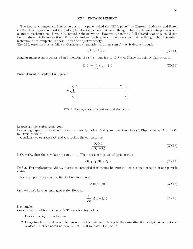
The idea of entanglement first came out in the paper called the “EPR paper” by Einstein, Podolsky, and Rosen(1935). This paper discussed the philosophy of entanglement but never thought that the different interpretations ofquantum mechanics could really be proved right or wrong. However a paper by Bell showed that they could andBell produced Bell’s inequalities. Einstein’s problem with quantum mechanics ws that he thought that “Quantummehanics is not complete, it doesn’t describe objective reality”.The EPR experiment is as follows. Consider a π0 particle which has spin J = 0. It decays through

π0 → e+ + e− (XXI.1)

Angular momentum is conserved and therefore the e+, e− pair has total J = 0. Hence the spin configuration is

|0, 0〉 =1√2

(↑↓ − ↓↑) (XXI.2)

Entanglement is displayed in figure 8

e+e-zz

zx x

50%

xx

FIG. 8. Entanglement of a positron and elecron pair

Lecture 27 -November 25th, 2011Interesting paper: “Is the moon there when nobody looks? Reality and quantum theory”, Physics Today, April 1985,by David Mermin.

Consider two operators O1 and O2. Define the correlator as

〈O1O2〉√〈O2

1〉 〈O22〉

(XXI.3)

If O1 = O2, then the correlator is equal to 1. The most common use of correlators is

〈O(x1, t1)O(x1, t2)〉 (XXI.4)

Def 3. Entanglement: We say a state is entangled if it cannot be written a as a simple product of one particlestates.

For example: If we could write the Helium atom as

ψ1(x)ψ2(x) (XXI.5)

then we don’t have an entangled state. However

1√2

(|↑↓〉 − |↓↑〉) (XXI.6)

is entangled.Consider a box with a button on it There a few key points

1. Brick stops light from flashing

2. Everytime both random number generators has pointers pointing in the same direction we get perfect anticor-relation. In order words we have GR or RG if we have 11,22, or 33.

52

G RG R

1

2 3

3 Switch Positions2 Lights

L R

1

2 3

FIG. 9. Entanglement figure

3. There are four possible outcomes

4. If one pays attention to the point directions then half the time we have GG or RR and half the time we haveGR and RG

Classical point of view says that particles have genes. In order for the paricles to have perfect anticorrelation werequire the particles 1 and 2 have the following gene table.

Particle one genes Particle two genes

123 123

GGG RRR

GGR RRG

GRG RGR

RGG GRR

RRG GGR

RGR GRG

GRR RGG

RRR GGG

Consider the GGR -RRG row. There are 9 possible pointer settings:

11, 12, 21, 22, 33

13, 23, 31, 32

The top row gives anti-correlation while the bottom row gives the same colours. For this gene the probably is 5/9 foranti-correlation. The row that we analyzed is the same form as all the rows but the first and law ones. On row 1 androw 8 we get perfect anti-correlation. Therefore identical results for 6 of the 8 rows (genes) and perfect anti-correlationfor the other two rows.

The classical conclusion is that if we pay no attention to pointer positions we will get anti-correlation with aprobabilty greater then 5/9. This is the simplest way to state Bell’s inequality. The experiment violates Bell’sinequality. This refutes the EPR claim of the existence of an element of physical reality.

The EPR reality criteria is:“If without in any way disturbing the system we can predict with certainty the value ofa physical quantity then there exists an element of physical reality corresponding to this physical quantity.”Recall

π0 → χ =1√2

(|↑↓〉 − |↓↑〉) (XXI.7)

53

Recall that

J2χ = 0χ (XXI.8)

We want to know that correlator:

〈χ|Sz1Sz2 |χ〉 (XXI.9)

First lets do the simpler correlator

Sz1Sz2 |↑↓〉 = −~2 1

2

1

2|↑↓〉 (XXI.10)

Sz1Sz2 |↓↑〉 = −~2

4|↓↑〉 (XXI.11)

Now

Sz1Sz2χ = −~2

4(XXI.12)

We can finally compute the normalized correlator:

〈χ|Sz1Sz2 |χ〉√〈χ| (Sz1 )

2 |χ〉 〈χ| (Sz2 )2 |χ〉

= −1 (XXI.13)

This tells you that the spins in this state are perfectly anti-correlated. Now consider the operators in the x direction

〈χ|Sx1Sx2 |χ〉√〈χ| (Sx1 )

2 |χ〉 〈χ| (Sx2 )2 |χ〉

(XXI.14)

To get this correlator we need

Sx1Sx2 |↑↓〉 =

~2

4|↓↑〉 (XXI.15)

Sx1Sx2 |↑↓〉 =

~2

4|↓↑〉 (XXI.16)

Sx1Sx2 |↓↑〉 =

~2

4|↑↓〉 (XXI.17)

Sx1Sx2χ = −~2

4χ (XXI.18)

Thus

〈χ|Sx1Sx2 |χ〉√〈χ| (Sx1 )

2 |χ〉 〈χ| (Sx2 )2 |χ〉

= −1 (XXI.19)

The same is true for the Sy1Sy2 we have perfect anti-correlation.

C (Sx1Sz2 ) |↑↓〉 = (Sx1 ↑) (Sz2 ) (XXI.20)

=~2

(0 1

1 0

)(1

0

)~2

(1 0

0 −1

)(0

1

)(XXI.21)

= −~2

4|↓↓〉 (XXI.22)

Similarly

Sx1Sz2 |↓↑〉 =

~2

4|↑↑〉 (XXI.23)

54

Sx1Sz2χ = −~2

4

1√2

(↓↓ + ↑↑) (XXI.24)

|χ|Sx1Sz2 |χ〉 = 0 (XXI.25)

Hence there is no correlation.

Lecture 28 - November 30th, 2011Recall the EPR experiment:

π0 → e+ + e− (XXI.26)

The results were

1. If the spin measurements are on the same axis then perfect anti-correlation

2. If you don’t pay attention to which axis then no-corelation

Classical thinking:If you construct gene tables to satisfy the first condition then the second condition will produce correlation.Quantum thinking :

π0 → 1√2

(↑↓ − ↓↑) ≡ χ; J = 0, Jz = 0 (XXI.27)

The three pointers in the experiment are actually the directions in which we are actually meauring the spin: The

vectors are (n1 = ez, n2 =√

32 ex −

12 ez, n3 = −

√3

2 ex −12 ez). Recall the definition of S

S =~2σ (XXI.28)

Where σ1 is the spin matrix corresponding to particle 1. To find the correlator we first find the relations:

Sz1Sz2 ↑↓=

−~2

4↑↓ (XXI.29)

The correlator of S1 · n1S2 · n1 (without normalization) is

〈χ|S1 · n1S2 · n1 |χ〉 = 〈χ|Sz1Sz2 |χ〉 (XXI.30)

= −1 (XXI.31)

Now lets calculate

〈χ| (S1 · n2) (S2 · n2) |χ〉 = 〈χ|

(√3

2Sx1 −

1

2Sz1

)(√3

2Sx2 −

1

2Sz2

)|χ〉 (XXI.32)

= 〈χ| 34Sx1S

x2 +

1

4Sz1S

z2 −√

3

4Sz1S

x2 −√

3

4Sx1S

z2 |χ〉 (XXI.33)

Define this operator in the bracket as O.

Sx =~2

(0 1

1 0

)(XXI.34)

Sx ↑ =~2

(0 1

1 0

)(1

0

)(XXI.35)

~2

(0

1

)(XXI.36)

55

Sx ↓ = − ↑ (XXI.37)

O ↑↓ =~2

4

(3

4↓↑ −1

4↑↓ −

√3

4↑↑ +

√3

4↓↓

)(XXI.38)

O ↓↑ =~2

4

(3

4↑↓ −1

4↓↑ +

√3

4↓↓ −

√3

4↑↑

)(XXI.39)

Finally

Oχ = O 1√2

(↑↓ − ↓↑) (XXI.40)

= −~2

4χ (XXI.41)

Thus these are perfectly anti-correlated.If we don’t pay any attention to the spin then we should get zero for the following: (i 6= j)∑

i,j

〈χ|S1 · niS2 · nj |χ〉 = 〈χ|∑i

S1 · ni∑j

S2 · nj |χ〉 (XXI.42)

= 〈χ|S1 ·

(∑i

ni

)S2 ·

∑j

nj

|χ〉 (XXI.43)

= 0 (XXI.44)

Since the vector sum over all the three vectors is trivially zero. To summarize: Bell’s inequality follows from classicalthinking. Bell’s inequality is violated by experiment and quantum mechanics. Bell’s inequality is a statistical state-ment. In other words you have to do many measurements and sum the results. This is the way things stood untilGHZ came along (Greenburger, Horne, and Zolnger) and they proposed an experiment and carried it out which isnot a statistical experiment (one-shot experiment). In this experiment 100% of the time quantum mechanics predictsone thing and classical mechanics predicts another. You are responsible for this experiment for the exam.We have solved most of the exactly solvable problems in quantum mechanics but we have approximation schemes forthe others.

• Time-dependant perturbation theory

• Time-independant perturbation thoery

• Degenerate perturbation theory

• WKB approximation

• Variational method

Lecture 29 - December 1st, 2011

XXII. VARIATIONAL METHOD

This is an approximation technique. If |α〉 is some trial state to the equation:

Hψ = Eψ (XXII.1)

56

Then we consider

〈α |H|α〉 (XXII.2)

As an apprimation to the energy. To get the trial state we make an educated guess. There is no way we’ll get theexact solution. If we minimize

〈α|H |α〉 (XXII.3)

this quantity with respect to a parameter then we assured of getting as closed as possilbe the exact solution. Mathe-matically:

d 〈α|H |α〉da

= 0 (XXII.4)

For some parameter a is the best possible solution. We call a a variational parameter and we use it to parametrizeour wavefunction. e.g. ψ(x, a). Why does it work? This works because

|α〉 =∑n

an |n〉 (XXII.5)

〈α|H |α〉 =∑n,n′

ana∗n′ 〈n′|H |n〉 (XXII.6)

but since this is an exact solution H |n〉 = En |n〉

〈α |H|α〉 =∑n,n′

a∗nan′Enδn,n′ =∑n

|an|2En (XXII.7)

≥ Eo∑n

|an|2 (XXII.8)

≥ Eo (XXII.9)

Mimizing the energy is maximizing ao. As an example consider Hydrogen− ~2

2m

(1

r

d2r

dr2

)+

1

2m

L2

r2− Ze2

r

ψ(r, φ, θ) = Eψ(r, φ, θ) (XXII.10)

Because the problem has rotational symmetry we know that ψ(r, φ, θ) = R(r)Ylm(φ, θ). Subsituting in we will get

H = − ~2

2m

(1

r

d2r

dr2

)+

~2

2mr2l (l + 1)− Ze2

r(XXII.11)

We will discuss l = 0. Thus

H = − ~2

2m

(1

r

d2r

dr2

)− Ze2

r(XXII.12)

Our trial solution is R(r) = 2(

1a

)3/2e−r/a, where a is the variational parameter (not ao). This is silly since we know

that R(r) above contains within it the exact solution. Note once we decide we want to try an exponential solution weare essentially forced to this form by dimensions and normalization (even the 2!). First lets find this (define γ in thisway).

HR(r) =

(− ~2

2m

(1

4

d2r

dr2

)− Ze2

r

)γe−r/a (XXII.13)

= γ

(− ~2

2m

(− 2

ar+

1

a2

)− Z e

2

r

)e−r/a (XXII.14)

〈a|H |a〉 =

∫ ∞o

γ2r2dr

(− ~2

2m

(− 2

ar+

1

a2

)− Z e

2

r

)e−r/a (XXII.15)

=4

a3

∫ ∞0

((~2

ma− Z e

2

r

)re−r/a − ~2

2ma2r2e−r/a

)dr (XXII.16)

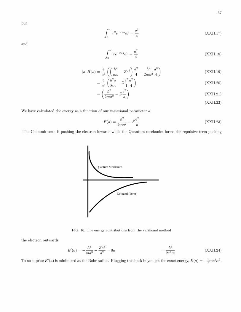
57

but ∫ ∞0

r2e−r/adr =a3

4(XXII.17)

and ∫ ∞0

re−r/adr =a2

4(XXII.18)

〈a|H |a〉 =4

a3

((~2

ma− Ze2

)a2

4− ~2

2ma2

a3

4

)(XXII.19)

=4

a3

(~2a

8m− Z e

2

1

a2

4

)(XXII.20)

=

(~2

2ma2− Z e

2

a

)(XXII.21)

(XXII.22)

We have calculated the energy as a function of our variational parameter a.

E(a) =~2

2ma2− Z e

2

a(XXII.23)

The Coloumb term is pushing the electron inwards while the Quantum mechanics forms the repulsive term pushing

Coloumb Term

Quantum Mechanics

FIG. 10. The energy contributions from the varitional method

the electron outwards.

E′(a) = − ~2

ma3+Ze2

a2= 0a =

~2

2e2m(XXII.24)

To no suprise E′(a) is minimized at the Bohr radius. Plugging this back in you get the exact energy, E(a) = − 12mc

2α2.