Quantum mechanics from symmetry and statistical

modelling.

Inge S. Helland∗

Department of MathematicsUniversity of Oslo.

Abstract

A version of quantum theory is derived from a set of plausible assumptionsrelated to the following general setting: For a given system there is a set ofexperiments that can be performed, and for each such experiment an ordinarystatistical model is defined. The parameters of the single experiments are func-tions of a hyperparameter, which defines the state of the system. There is asymmetry group acting on the hyperparameters, and for the induced action onthe parameters of the single experiment a simple consistency property is as-sumed, called permissibility of the parametric function. The other assumptionsneeded are rather weak. The derivation relies partly on quantum logic, partlyon a group representation of the hyperparameter group, where the invariantspaces are shown to be in 1-1 correspondence with the equivalence classes ofpermissible parametric functions. Planck’s constant only plays a role connectedto generators of unitary group representations.

Keywords: Permissible parameters; quantum logic; quantum theory; statistical mod-els; symmetry.

∗University of Oslo, Department of Mathematics, P.O.Box 1053 Blindern, N-0316 Oslo, Norway.E-mail: ingeh@math.uio.no

1

1 Introduction.

The two great revolutions in physics at the beginning of this century - relativityand quantum mechanics - still influence nearly all aspects of theoretical physics.Similar as they may be, both in their impact on modern science and in the way theyin their time turned conventional ideas upside down, there are also of course greatdifferences - both in origin, appearance and type of content. Relativity theory wasfounded by one man, Einstein, while the ideas of quantum theory developed overtime through the work of many people, most notably Planck, Bohr, Schrodinger,Heisenberg, Pauli and Dirac. An equally important - and perhaps related - aspect,is the following: Relativity theory can be developed logically from a few intuitivelyclear, nearly obvious, concepts and axioms, essentially only constancy of the speedof light and invariance of physical laws under change of coordinate system, whilequantum theory still has a rather awkward foundation in its abstract concepts forstates and observables.

During the years, several attempts of a deeper foundation of quantum theoryhave been made; some of these we will return to later. Although there is far from auniversal agreement on the foundation, today’s physicists, both theoretical and ex-perimental, have developed a clear intuition directly connected to states of a systemas rays in a complex Hilbert space and observables as selfadjoint operators in thesame space. The theory has had success in very many fields - some claim that quan-tum theory is the most successfull physical theory ever advanced, but it has also metproblems: Difficulties with defining the border between object and observer in vonNeuman’s quantum measurement theory; difficulties with interpretations requiringmany worlds or action at a distance; infinities in quantum field theory requiring com-plicated renormalization programs; difficulties in reconciling the theory with generalrelativity and so on. We will of course not try to attack all these problems here.What we will assert, though, is that the fact that such difficulties occur, does makeit legitimate to look at the foundation of the theory with fresh eyes again. One wayto do this, is to try to find a foundation which is in accordance with common sense.Another way is to compare it with another, apparently unrelated, theoretical area.In this paper we will try to combine both these lines of attack.

A vital clue is the role of probability in quantum theory. In the beginning, thiswas an aspect that overshadowed all other difficulties in the theory, and that madeleading physicists - first of them Einstein himself - sceptical: The new physical lawswere then and are still claimed to be probabilistic by necessity. Still some people arelooking at hidden variable theories in attempts to avoid the fact that the fundamentallaws of nature are stochastic, but after the experiments of Aspect et al. (1982) andother overwhelming evidence, most scientists seem to accept stochasticity of natureas an established fact.

2

At the same time, statistical science has developed methodology that has foundapplications in an increasing number of empirical sciences, methodology largely basedupon stochastic modelling. With this background, the obvious, but apparently verydifficult question then is: Why has there been virtually no scientific contact betweenphysicists and statisticians throughout this century? This lack of contact is in factvery striking. At the same time as Dirac was developing a foundation for relativis-tic quantum theory in Cambridge in England, R.A. Fisher completely independentlydeveloped the foundation of statistical inference theory based upon probability mod-els in Rothamsted and London. While modern quantum field theory was developedby Feynman in Princeton and Schwinger in Harvard, J. Neyman and coworkers laythe foundation of modern statistical inference theory in Berkeley. One of the fewearly contacts that I know of is Feynman’s (1951) Berkeley Symposium paper onthe interpretation of probabilities in quantum mechanics. Today, quantum theorysometimes has its own session at large international statistical conferences, but thelanguage spoken there is of a nature which is difficult to understand for ordinarystatisticians. Meyer’s (1993) book on non-commutative probability theory may beseen as an attempt to make a synthesis of the two worlds, but this book does notaddress the foundation question if we seek a foundation related to common sense. Itis also becoming increasingly apparent that there are similarities between advancedprobability theory and quantum theory, but these similarities seem to be mostly atthe formal level.

The lack of a common ground for modern physics and statistics is even moresurprising when we know that the outcome of any single experiment with fixedexperimental arrangement can always be described by ordinary probability models,also in the world of particle physics. It is in cases where several arrangements arepossible, as when one has the choice between measuring position and momentum of aparticle, that quantum mechanics gives results which cannot be reached by ordinaryprobability theory. In addition, quantum theory gives definite rules for computingprobabilities, also in cases where the ordinary probability concept can be used inprinciple.

We will formulate below an extended experimental setting, which includes thepossible decisions which must be made before the experiment itself is carried out, atleast before the final inference is made. We will look at the situation where strongsymmetries exist both within the single experiments and in the wider experimentalsetting between the single experiments. This, together with other reasonable as-sumptions, will lead to probability models of the type found in ordinary quantummechanics.

The physical implications of this theory, at least in its non-relativistic variant arenot expected to differ considerably from existing quantum theory. Questions relatedto mathematical equivalence will be discussed later. An interesting further challenge

3

may be the question of finding a corresponding relativistic theory. This issue will notbe pursued here, but in light of the importance of symmetry groups in high energyphysics, it seems very plausible that it should be possible to develop the approachin this direction, too. A brief discussion on this will be given in the last section.

Our aim is to write the paper in such a way that the principal ideas can be ap-preciated both by theoretical physisists, mathematicians and statisticians. Technicaldetails at several points are unavoidable, however. Also, even though we will try tobe fairly precise, at least in the main results, there may still be room for improve-ment in mathematical rigor. What we feel are the most important assumptions, arestated explicitly. Minor technical assumptions are stated in the text.

The discussion of this paper is continued in Helland (1999), where we among otherthings give a more explicit construction of the basic Hilbert space, a constructionwhich is independent of the apparatus of quantum logic.

2 Experimental setting.

The common statistical framework for analyzing an experiment is a sample space X ,listing the possible experimental outcomes, a fixed σ-algebra (Boolean algebra) Fof subsets of X , and a class {Pθ; θ ∈ Θ} of probability measures on the measurablespace (X ,F). The parameter θ - or a function of this parameter - is ordinarily theunknown quantity which the statistician aims at saying something about using theoutcome of the experiment. A fixed θ, or alternatively, a probability distributionexpressing prior knowledge about θ, may also be related to the phycisist’s concept of‘state’. A simple purpose of a statistical experiment might be to estimate θ, whichformally means to select a function θ on the sample space X such that θ(x) is areasonable estimate of θ when the observation x is given. There is a considerableliterature on statistical inference; three good and thorough books with differentperspectives are Berger (1985), Lehmann (1983) and Cox and Hinkley (1974). Bothat the more specialized and at the more elementary level there are very many books,of course. An important point is that intuition related to statistical methodology inthis ordinary sense has been developed in a large number of empirical sciences, alsoin parts of experimental physics.

A very general approach to statistics assumes a decision theoretical framework:First, a space D of possible decisions is defined, given the experimental outcome; forinstance, D can consist of different estimators of θ. Then a loss function L(θ, d(·)) isspecified, giving the loss by taking the decision d when the true parameter is θ. Thechoice of decision is typically done by minimizing the expected loss. By restrictingthe class of decision functions so that they posess invariance properties, or so that

4

estimators have the correct expectation, this can often be done uniformly over theunknown parameter. Another possible course - gaining increasing popularity - isto assume a prior probability distribution over the parameter space, and then baseinference on the corresponding posterior distribution, given the data. This is calledthe Bayesian approach.

Essential for what follows, is that we will extend the traditional statistical frame-work to include possible actions taken by an experimenter before or during a givenexperiment. The most important actions for our purposes are those that label thewhole experiment, and thus allows different experiments to be done in the samesituation. However, we will also allow actions that change the class of probabilitymeasures, the space of decisions and/ or the loss function.

Thus we start with a space A of possible actions, and for each a ∈ A we havean experiment Ea, consisting of a probability model (Xa,Fa, {P aθ ; θ ∈ Θa}), andpossibly a loss function La(·, ·) and a space Da of potential decisions. In macroscopicexperiments such actions are in fact very common. They are not usually explicitlytaken into account in the statistical analysis, but are taken as fixed once and for all,an attitude which is fairly obvious in some cases, but absolutely can be discussed inother cases. In fact, more can be said, also in the ordinary statistical setting, for acloser link between the experimental design phase (choosing a) and the statisticalanalysis phase. A partial list of possibilities for choosing a include:

(a) Choice between a number of essentially different experiments that are possibleto perform in a given situation.

(b) Choice of target population, and way to select experimental units, includingchoice of randomization. Choice of conditioning in models is related to these issues.

(c) Choice of treatments. Here are many variants: There are lots of examples ofmedical treatments which are mutually exclusive. In factorial experiments the choiceof factors and the levels of these are important issues.

(d) A choice between different statistical models; for instance, one may want toreduce the number of parameters if the model is to complicated to give firm decisions.In fact, this is permissible under certain conditions.

One main purpose of this paper will be to explore the relationship between macro-scopic statistical modelling and the microscopic modelling we find in the quantummechanical world. In the latter one definitively has the choice between performingdifferent experiments, say, measuring position or moment or measuring spin in differ-ent directions. The quantum mechanical state of a particle or a particle system canbe used to predict the outcome of any given of these experiments, once the choice ismade. In this way one might say that the quantum mechanical state vector containsthe simultaneous model of a large set of possible statistical experiments Ea(a ∈ A).A major reason why this is possible, is that the situation contains a high degree of

5

symmetry. To study the connection between quantum mechanics and statistics moredirectly, it turns out, however, to be useful first to consider a simpler representationthan the ordinary Hilbert space representation of quantum mechanics.

3 The lattice approach to quantum theory.

Mathematically, a σ-lattice is defined as a partially ordered set L such that the infi-mum and supremum (with respect to the given ordering) of every countable subsetexist and belong to L. In this section we will summarize the approach to quantummechanics taking lattices of propositions as points of departure. These can be lookedupon as generalizations of the σ-algebras of classical probability, where the propo-sitions are subsets of a given space X , ordered by set inclusion; the term Booleanalgebra is sometimes used for the same concept. For Boolean algebras, the par-tial ordering corresponds to set inclusion, and infimum and supremum correspondsto intersection and union, respectively. In the following we will mainly consider(complete) lattices, where the infimum and supremum of all subsets, not only thecountable ones, exist.

The lattice approach to quantum mechanics consists of formulating a number ofaxioms for a lattice which is weaker than the set of axioms needed to define a Booleanalgebra, just sufficiently weak that they are satisfied by the set of projections in aHilbert space, which are the entities that represent propositions in conventionalquantum mechanics. We will follow largely Beltrametti and Cassinelli (1981) inpresenting these axioms. It is relatively easy to prove that the axioms below actuallyare satisfied by Hilbert space projections, much more difficult to show that theaxioms by necessity imply that the lattice has a Hilbert space representation. Weproceed with the necessary definitions; in the next section we will try to relate thesedefinitions to sets of potential experiments as formulated above.

We have already defined a lattice L as a set of propositions {P} with a partialordering ≤ such that the supremum

∨i Pi exists and belongs to L when all the Pi

belong to L, similarly for infimum. (∨i Pi is defined as a proposition P such that

Pi ≤ P for all Pi, and such that Pi ≤ P0 for all Pi implies P ≤ P0. It is easy to showthat the supremum, if it exists, is unique if the lattice is assumed to have the propertythat P1 ≤ P2 and P2 ≤ P1 implies P1 = P2. Infimum is defined correspondingly.)

It follows that L contains the infimum of all propositions, denoted 0, and thesupremum of all propositions, denoted 1.

What corresponds to the complement in a Boolean algebra, is here denoted byorthocomplement. An orthocomplementation in a lattice L is a mapping P → P⊥ of

6

L onto itself such that (i) P⊥⊥ = P, (ii) P1 ≤ P2 implies P⊥2 ≤ P⊥

1 , (iii) P ∧P⊥ = 0and (iv) P ∨ P⊥ = 1. It is easy to see that De Morgan’s laws follow from (ii):

(∨Pi)⊥ =

∧P⊥i , (

∧Pi)⊥ =

∨P⊥i .

Two propositions P1 and P2 are said to be disjoint or orthogonal, written P1 ⊥ P2

when P1 ≤ P⊥2 (or, equivalently, when P2 ≤ P⊥

1 ). A subset of L formed by pairwisedisjoint elements is simply called a disjoint subset. The lattice L is called separableif every disjoint subset of L is at most countable.

If P1 ≤ P2, we will write P2 − P1 for P2 ∧ P⊥1 . It is clear that we then have

P2 − P1 ⊥ P1. A lattice L is called orthomodular if P1 ≤ P2 implies P2 = P1 ∨(P2−P1). One other way to put this, is that the distributive laws hold for the triple(P1,P2,P⊥

1 ) when P1 ≤ P2.A much stronger requirement is that the distributive laws should hold for all

triples:

P1 ∨ (P2 ∧ P3) = (P1 ∨ P2) ∧ (P1 ∨ P3), P1 ∧ (P2 ∨ P3) = (P1 ∧ P2) ∨ (P1 ∧ P3).

An orthocomplemented distributive lattice is in general a Boolean algebra, and canalways be realized as an algebra of subsets of a fixed set.

The lattices of quantum mechanics are orthocomplemented, but nondistributive;they only satisfy the weaker requirement of being orthomodular. Much of the pio-neering work in the lattice approach to quantum mechanics is due to Mackey (1963).Two books on orthomodular lattices are Beran (1985) and Kalmbach (1983). Thisrepresents an approach to quantum mechanics that in some sense is more primitivethan most other approaches, but there are still concepts here, like the lattice prop-erty or orthomodularity, which are difficult to get an intuitive relation to. Our aimhere will be to try to understand these concepts to some extent in terms of ordi-nary statistical models for a set of potential experiments and in terms of symmetryproperties.

In addition to orthomodularity, two further properties are required by Beltram-etti and Cassinelli (1981): The lattices are assumed to be atomic and to have thecovering property.

A nonzero element P0 of L is called an atom if 0 ≤ P ≤ P0 implies P = 0 orP = P0. The lattice L is called atomic if there always for P 6= 0 exists an atom P0

such that P0 ≤ P. It can be shown that if L is an orthomodular, atomic lattice,then every element of L is the union of the atoms that it contains. If the lattice isseparable, this union is at most countable.

We say that L has the covering property if for every P1 in L and every atom P0

such that P1 ∧ P0 = 0, we have that P1 ≤ P2 ≤ P1 ∨ P0 implies either P2 = P1 orP2 = P1 ∨ P0.

7

In total, the kind of propositional structure which is promoted in Beltramettiand Cassinelli (1981) as a basis for quantum mechanics is an orthocomplemented,orthomodular, separable lattice which is atomic and has the covering property. Allthese requirements are proved to hold for the lattice of projection operators in aseparable Hilbert space, or equivalently, the lattice of all closed subspaces of theHilbert space.

One can also prove results in the opposite direction, though this is much moredifficult: If the given requirements hold for some lattice, then one can constructan isomorphic Hilbert space in the sense that the projections upon subspaces ofthis Hilbert space are in one-to-one correspondence with the propositions of thelattice, with corresponding ordering. The proof of this last result is only hinted atin Beltrametti and Cassinelli (1981); more details are given in Piron (1976) and inMaeda and Maeda (1970). Related results can also be found in Varadarajan (1985).One problem is to convince oneself that the complex number field is the natural tochoose as a basis for the Hilbert space: One can also construct representations basedon the real or quaternion number field.

Finally, the concept of state in Quantum mechanics can be defined as a probabil-ity measure on the propositions of a lattice. In the Hilbert space representation thefamous theorem of Gleason says that all states can be represented by density opera-tors ρ (positive operators with trace tr(ρ) = 1) in the sense that the expectation ofevery observator, represented by a selfadjoint operator A, is given by

tr(Aρ).

As is wellknown from probability theory, the set of expectations for all variablesdetermines the set of probability distributions for all variables.

4 A set of potential statistical experiments.

Let us start by turning to a completely different situation where the concept of‘state’ is also being used. Consider a medical patient. One way to make precisewhat is meant by the state of this patient is to contemplate the potential resultsof all possible tests that the patient can be exposed to, where the word ‘test’ isused in a very wide sense, possibly including treatments or parts of treatments.Thus in a concrete setting like this we can imagine a large number of potentialexperiments, some possibly mutually exclusive, and let the state be defined abstractlyas the totality of probability distributions of results from these experiments, or someparameter determining all these probability distributions. A similar concept can be

8

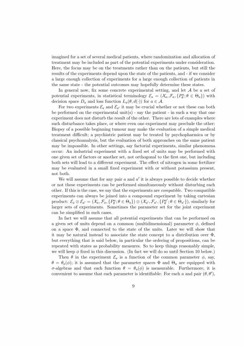
imagined for a set of several medical patients, where randomization and allocation oftreatment may be included as part of the potential experiments under consideration.Here, the focus may be on the treatments rather than on the patients, but still theresults of the experiments depend upon the state of the patients, and - if we considera large enough collection of experiments for a large enough collection of patients inthe same state - the potential outcomes may hopefully determine these states.

In general now, fix some concrete experimental setting, and let A be a set ofpotential experiments, in statistical terminology Ea = (Xa,Fa, {P aθ ; θ ∈ Θa}) withdecision space Da and loss function La(θ, d(·)) for a ∈ A.

For two experiments Ea and Ea′ it may be crucial whether or not these can bothbe performed on the experimental unit(s) - say the patient - in such a way that oneexperiment does not disturb the result of the other. There are lots of examples wheresuch disturbance takes place, or where even one experiment may preclude the other:Biopsy of a possible beginning tumour may make the evaluation of a simple medicaltreatment difficult; a psychiatric patient may be treated by psychopharmica or byclassical psychoanalysis, but the evaluation of both approaches on the same patientmay be impossible. In other settings, say factorial experiments, similar phenomenaoccur: An industrial experiment with a fixed set of units may be performed withone given set of factors or another set, not orthogonal to the first one, but includingboth sets will lead to a different experiment. The effect of nitrogen in some fertilizermay be evaluated in a small fixed experiment with or without potassium present,not both.

We will assume that for any pair a and a′ it is always possible to decide whetheror not these experiments can be performed simultaneously without disturbing eachother. If this is the case, we say that the experiments are compatible. Two compatibleexperiments can always be joined into a compound experiment by taking cartesianproduct: Ea ⊗ Ea′ = (Xa,Fa, {P aθ ; θ ∈ Θa}) ⊗ (Xa′ ,Fa′ , {P a′θ ; θ ∈ Θa′}), similarly forlarger sets of experiments. Sometimes the parameter set for the joint experimentcan be simplified in such cases.

In fact we will assume that all potential experiments that can be performed ona given set of units depend on a common (multidimensional) parameter φ, definedon a space Φ, and connected to the state of the units. Later we will show thatit may be natural instead to associate the state concept to a distribution over Φ,but everything that is said below, in particular the ordering of propositions, can berepeated with states as probability measures. So to keep things reasonably simple,we will keep φ fixed in this discussion. (In fact we will do so until Section 10 below.)

Then θ in the experiment Ea is a function of the common parameter φ, say,θ = θa(φ); it is assumed that the parameter spaces Φ and Θa are equipped withσ-algebras and that each function θ = θa(φ) is measurable. Furthermore, it isconvenient to assume that each parameter is identifiable: For each a and pair (θ, θ′),

9

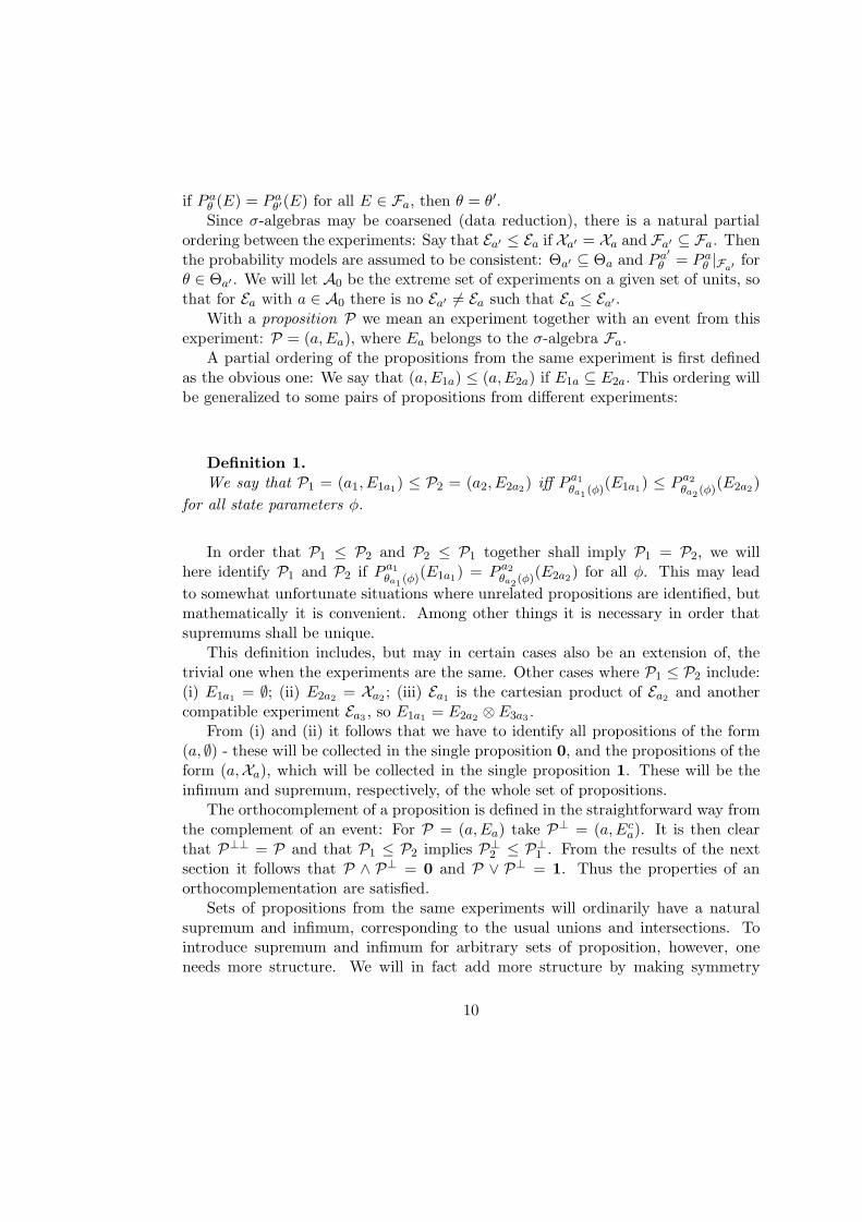
if P aθ (E) = P aθ′(E) for all E ∈ Fa, then θ = θ′.Since σ-algebras may be coarsened (data reduction), there is a natural partial

ordering between the experiments: Say that Ea′ ≤ Ea if Xa′ = Xa and Fa′ ⊆ Fa. Thenthe probability models are assumed to be consistent: Θa′ ⊆ Θa and P a

′θ = P aθ |Fa′ for

θ ∈ Θa′ . We will let A0 be the extreme set of experiments on a given set of units, sothat for Ea with a ∈ A0 there is no Ea′ 6= Ea such that Ea ≤ Ea′ .

With a proposition P we mean an experiment together with an event from thisexperiment: P = (a,Ea), where Ea belongs to the σ-algebra Fa.

A partial ordering of the propositions from the same experiment is first definedas the obvious one: We say that (a,E1a) ≤ (a,E2a) if E1a ⊆ E2a. This ordering willbe generalized to some pairs of propositions from different experiments:

Definition 1.We say that P1 = (a1, E1a1) ≤ P2 = (a2, E2a2) iff P a1θa1 (φ)(E1a1) ≤ P a2θa2 (φ)(E2a2)

for all state parameters φ.

In order that P1 ≤ P2 and P2 ≤ P1 together shall imply P1 = P2, we willhere identify P1 and P2 if P a1θa1 (φ)(E1a1) = P a2θa2(φ)(E2a2) for all φ. This may leadto somewhat unfortunate situations where unrelated propositions are identified, butmathematically it is convenient. Among other things it is necessary in order thatsupremums shall be unique.

This definition includes, but may in certain cases also be an extension of, thetrivial one when the experiments are the same. Other cases where P1 ≤ P2 include:(i) E1a1 = ∅; (ii) E2a2 = Xa2 ; (iii) Ea1 is the cartesian product of Ea2 and anothercompatible experiment Ea3 , so E1a1 = E2a2 ⊗ E3a3 .

From (i) and (ii) it follows that we have to identify all propositions of the form(a, ∅) - these will be collected in the single proposition 0, and the propositions of theform (a,Xa), which will be collected in the single proposition 1. These will be theinfimum and supremum, respectively, of the whole set of propositions.

The orthocomplement of a proposition is defined in the straightforward way fromthe complement of an event: For P = (a,Ea) take P⊥ = (a,Eca). It is then clearthat P⊥⊥ = P and that P1 ≤ P2 implies P⊥

2 ≤ P⊥1 . From the results of the next

section it follows that P ∧ P⊥ = 0 and P ∨ P⊥ = 1. Thus the properties of anorthocomplementation are satisfied.

Sets of propositions from the same experiments will ordinarily have a naturalsupremum and infimum, corresponding to the usual unions and intersections. Tointroduce supremum and infimum for arbitrary sets of proposition, however, oneneeds more structure. We will in fact add more structure by making symmetry

10

assumptions. But first we will show that the simple structure of sets of experimentsunder weak extra assumptions implies that the set of propositions always will be anorthocomplemented, orthomodular poset.

5 Orthomodular propositions from experiments.

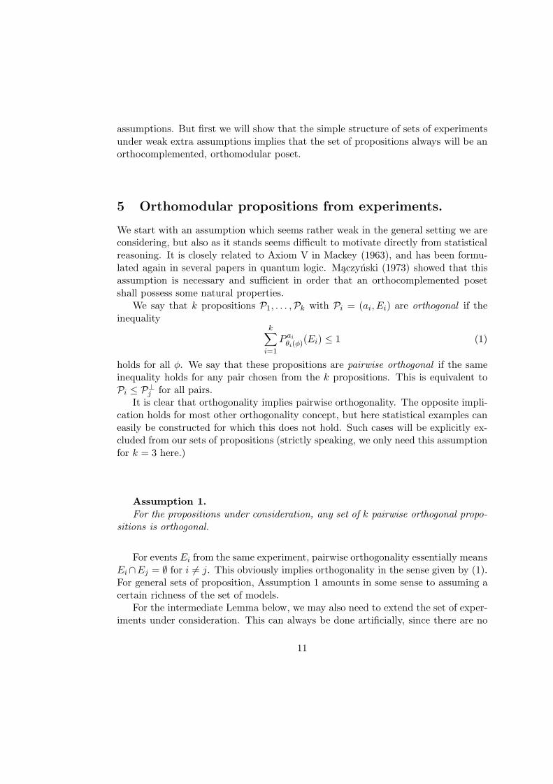
We start with an assumption which seems rather weak in the general setting we areconsidering, but also as it stands seems difficult to motivate directly from statisticalreasoning. It is closely related to Axiom V in Mackey (1963), and has been formu-lated again in several papers in quantum logic. Maczynski (1973) showed that thisassumption is necessary and sufficient in order that an orthocomplemented posetshall possess some natural properties.

We say that k propositions P1, . . . ,Pk with Pi = (ai, Ei) are orthogonal if theinequality

k∑i=1

P ai

θi(φ)(Ei) ≤ 1 (1)

holds for all φ. We say that these propositions are pairwise orthogonal if the sameinequality holds for any pair chosen from the k propositions. This is equivalent toPi ≤ P⊥

j for all pairs.It is clear that orthogonality implies pairwise orthogonality. The opposite impli-

cation holds for most other orthogonality concept, but here statistical examples caneasily be constructed for which this does not hold. Such cases will be explicitly ex-cluded from our sets of propositions (strictly speaking, we only need this assumptionfor k = 3 here.)

Assumption 1.For the propositions under consideration, any set of k pairwise orthogonal propo-

sitions is orthogonal.

For events Ei from the same experiment, pairwise orthogonality essentially meansEi∩Ej = ∅ for i 6= j. This obviously implies orthogonality in the sense given by (1).For general sets of proposition, Assumption 1 amounts in some sense to assuming acertain richness of the set of models.

For the intermediate Lemma below, we may also need to extend the set of exper-iments under consideration. This can always be done artificially, since there are no

11

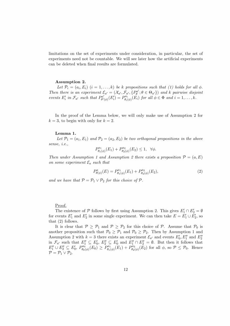
limitations on the set of experiments under consideration, in particular, the set ofexperiments need not be countable. We will see later how the artificial experimentscan be deleted when final results are formulated.

Assumption 2.Let Pi = (ai, Ei) (i = 1, . . . , k) be k propositions such that (1) holds for all φ.

Then there is an experiment Ea′ = (Xa′ ,Fa′ , {P a′θ ; θ ∈ Θa′}) and k pairwise disjointevents E′

i in Fa′ such that P a′

θ′(φ)(E′i) = P ai

θi(φ)(Ei) for all φ ∈ Φ and i = 1, . . . , k.

In the proof of the Lemma below, we will only make use of Assumption 2 fork = 3, to begin with only for k = 2.

Lemma 1.Let P1 = (a1, E1) and P2 = (a2, E2) be two orthogonal propositions in the above

sense, i.e.,P a1θ1(φ)(E1) + P a2θ2(φ)(E2) ≤ 1, ∀φ.

Then under Assumption 1 and Assumption 2 there exists a proposition P = (a,E)on some experiment Ea such that

P aθ(φ)(E) = P a1θ1(φ)(E1) + P a2θ2(φ)(E2), (2)

and we have that P = P1 ∨ P2 for this choice of P.

Proof.The existence of P follows by first using Assumption 2. This gives E′

1 ∩ E′2 = ∅

for events E′1 and E′

2 in some single experiment. We can then take E = E′1 ∪E′

2, sothat (2) follows.

It is clear that P ≥ P1 and P ≥ P2 for this choice of P. Assume that P0 isanother proposition such that P0 ≥ P1 and P0 ≥ P2. Then by Assumption 1 andAssumption 2 with k = 3 there exists an experiment Ea′ and events E′

0, E′′1 and E′′

2

in Fa′ such that E′′1 ⊆ E′

0, E′′2 ⊆ E′

0 and E′′1 ∩ E′′

2 = ∅. But then it follows thatE′′

1 ∪ E′′2 ⊆ E′

0, Pa0θ0(φ)(E0) ≥ P a1θ1(φ)(E1) + P a2θ2(φ)(E2) for all φ, so P ≤ P0. Hence

P = P1 ∨ P2.

12

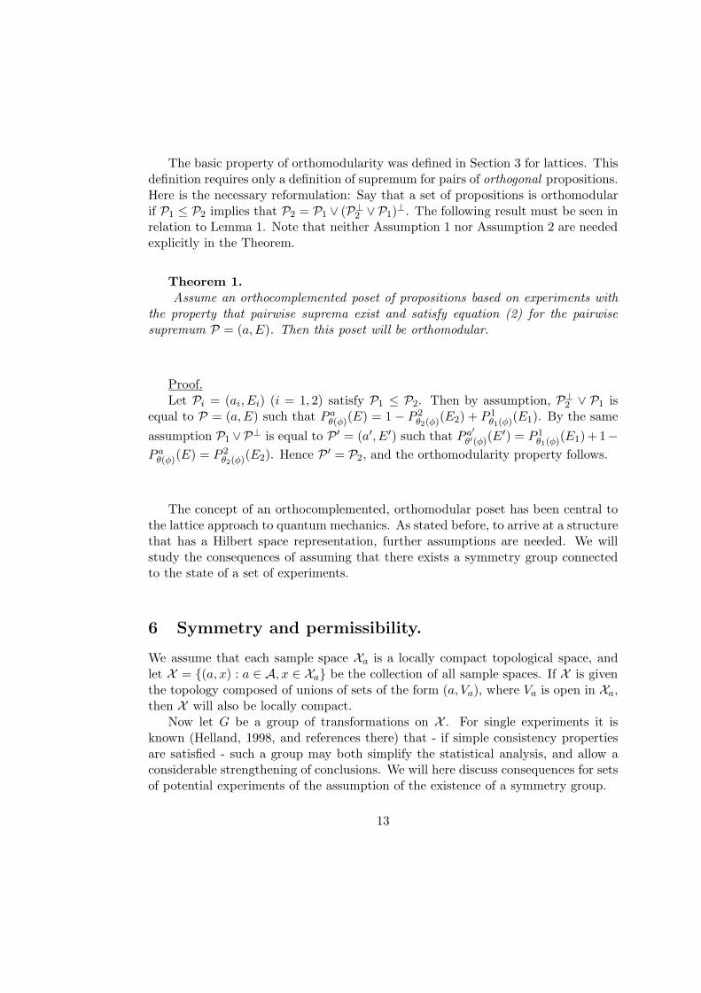
The basic property of orthomodularity was defined in Section 3 for lattices. Thisdefinition requires only a definition of supremum for pairs of orthogonal propositions.Here is the necessary reformulation: Say that a set of propositions is orthomodularif P1 ≤ P2 implies that P2 = P1 ∨ (P⊥

2 ∨P1)⊥. The following result must be seen inrelation to Lemma 1. Note that neither Assumption 1 nor Assumption 2 are neededexplicitly in the Theorem.

Theorem 1.Assume an orthocomplemented poset of propositions based on experiments with

the property that pairwise suprema exist and satisfy equation (2) for the pairwisesupremum P = (a,E). Then this poset will be orthomodular.

Proof.Let Pi = (ai, Ei) (i = 1, 2) satisfy P1 ≤ P2. Then by assumption, P⊥

2 ∨ P1 isequal to P = (a,E) such that P aθ(φ)(E) = 1− P 2

θ2(φ)(E2) + P 1θ1(φ)(E1). By the same

assumption P1 ∨P⊥ is equal to P ′ = (a′, E′) such that P a′

θ′(φ)(E′) = P 1

θ1(φ)(E1)+ 1−P aθ(φ)(E) = P 2

θ2(φ)(E2). Hence P ′ = P2, and the orthomodularity property follows.

The concept of an orthocomplemented, orthomodular poset has been central tothe lattice approach to quantum mechanics. As stated before, to arrive at a structurethat has a Hilbert space representation, further assumptions are needed. We willstudy the consequences of assuming that there exists a symmetry group connectedto the state of a set of experiments.

6 Symmetry and permissibility.

We assume that each sample space Xa is a locally compact topological space, andlet X = {(a, x) : a ∈ A, x ∈ Xa} be the collection of all sample spaces. If X is giventhe topology composed of unions of sets of the form (a, Va), where Va is open in Xa,then X will also be locally compact.

Now let G be a group of transformations on X . For single experiments it isknown (Helland, 1998, and references there) that - if simple consistency propertiesare satisfied - such a group may both simplify the statistical analysis, and allow aconsiderable strengthening of conclusions. We will here discuss consequences for setsof potential experiments of the assumption of the existence of a symmetry group.

13

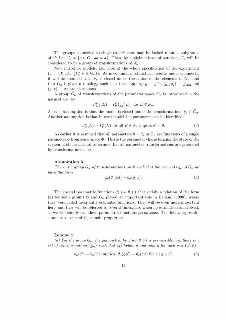
The groups connected to single experiments may be looked upon as subgroupsof G: Let Ga = {g ∈ G : ga = a}. Then, by a slight misuse of notation, Ga will beconsidered to be a group of transformations of Xa.

Now introduce models, i.e., look at the whole specification of the experimentEa = (Xa,Fa, {P aθ ; θ ∈ Θa}). As is common in statistical models under symmerty,it will be assumed that Fa is closed under the action of the elements of Ga, andthat Ga is given a topology such that the mappings g → g−1, (g1, g2) → g1g2 and(g, x) → gx are continuous.

A group Ga of transformations of the parameter space Θa is introduced in thenatural way by

P agaθ(E) = P aθ (g−1a E) for E ∈ Fa.

A basic assumption is that the model is closed under the transformations ga ∈ Ga.Another assumption is that in each model the parameter can be identified:

P aθ′(E) = P aθ (E) for all E ∈ Fa implies θ′ = θ. (3)

As earlier it is assumed that all parameters θ = θa in Θa are functions of a singleparameter φ from some space Φ. This is the parameter characterizing the state of thesystem, and it is natural to assume that all parameter transformations are generatedby transformations of φ.

Assumption 3.There is a group Ga of transformations on Φ such that the elements ga of Ga all

have the formga(θa(φ)) = θa(gaφ). (4)

The special parametric functions θ(·) = θa(·) that satisfy a relation of the form(4) for some groups G and Ga played an important role in Helland (1998), wherethey were called invariantly estimable functions. They will be even more importanthere, and they will be referred to several times, also when no estimation is involved,so we will simply call these parametric functions permissible. The following resultssummarize some of their main properties:

Lemma 2.(a) For the group Ga, the parametric function θa(·) is permissible, i.e, there is a

set of transformations {ga} such that (4) holds, if and only if for each pair (φ′, φ)

θa(φ′) = θa(φ) implies θa(gφ′) = θa(gφ) for all g ∈ G. (5)

14

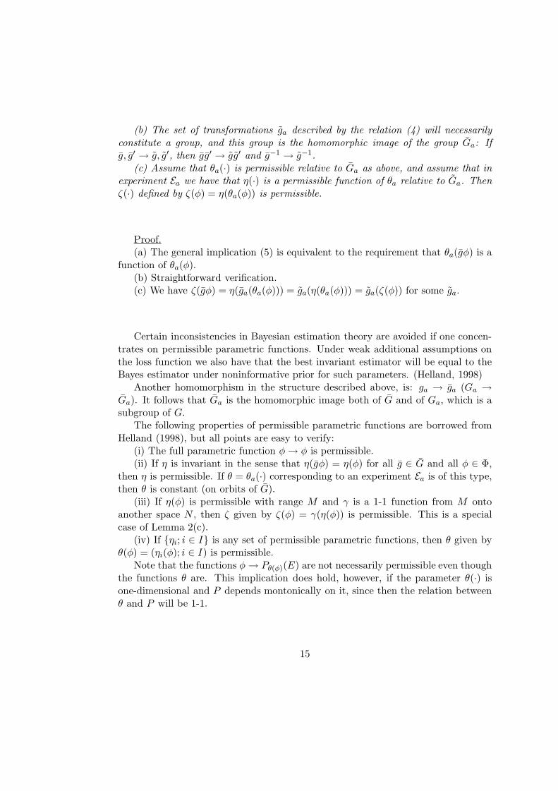
(b) The set of transformations ga described by the relation (4) will necessarilyconstitute a group, and this group is the homomorphic image of the group Ga: Ifg, g′ → g, g′, then gg′ → gg′ and g−1 → g−1.

(c) Assume that θa(·) is permissible relative to Ga as above, and assume that inexperiment Ea we have that η(·) is a permissible function of θa relative to Ga. Thenζ(·) defined by ζ(φ) = η(θa(φ)) is permissible.

Proof.(a) The general implication (5) is equivalent to the requirement that θa(gφ) is a

function of θa(φ).(b) Straightforward verification.(c) We have ζ(gφ) = η(ga(θa(φ))) = ga(η(θa(φ))) = ga(ζ(φ)) for some ga.

Certain inconsistencies in Bayesian estimation theory are avoided if one concen-trates on permissible parametric functions. Under weak additional assumptions onthe loss function we also have that the best invariant estimator will be equal to theBayes estimator under noninformative prior for such parameters. (Helland, 1998)

Another homomorphism in the structure described above, is: ga → ga (Ga →Ga). It follows that Ga is the homomorphic image both of G and of Ga, which is asubgroup of G.

The following properties of permissible parametric functions are borrowed fromHelland (1998), but all points are easy to verify:

(i) The full parametric function φ→ φ is permissible.(ii) If η is invariant in the sense that η(gφ) = η(φ) for all g ∈ G and all φ ∈ Φ,

then η is permissible. If θ = θa(·) corresponding to an experiment Ea is of this type,then θ is constant (on orbits of G).

(iii) If η(φ) is permissible with range M and γ is a 1-1 function from M ontoanother space N , then ζ given by ζ(φ) = γ(η(φ)) is permissible. This is a specialcase of Lemma 2(c).

(iv) If {ηi; i ∈ I} is any set of permissible parametric functions, then θ given byθ(φ) = (ηi(φ); i ∈ I) is permissible.

Note that the functions φ→ Pθ(φ)(E) are not necessarily permissible even thoughthe functions θ are. This implication does hold, however, if the parameter θ(·) isone-dimensional and P depends montonically on it, since then the relation betweenθ and P will be 1-1.

15

7 Group representation related to the parameter space.

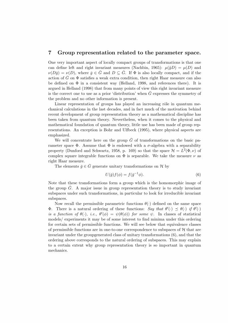
One very important aspect of locally compact groups of transformations is that onecan define left and right invariant measures (Nachbin, 1965): µ(gD) = µ(D) andν(Dg) = ν(D), where g ∈ G and D ⊆ G. If Φ is also locally compact, and if theaction of G on Φ satisfies a weak extra condition, then right Haar measure can alsobe defined on Φ in a consistent way (Helland, 1998, and references there). It isargued in Helland (1998) that from many points of view this right invariant measureis the correct one to use as a prior ‘distribution’ when G expresses the symmetry ofthe problem and no other information is present.

Linear representation of groups has played an increasing role in quantum me-chanical calculations in the last decades, and in fact much of the motivation behindrecent development of group representation theory as a mathematical discipline hasbeen taken from quantum theory. Nevertheless, when it comes to the physical andmathematical foundation of quantum theory, little use has been made of group rep-resentations. An exception is Bohr and Ulfbeck (1995), where physical aspects areemphasized.

We will concentrate here on the group G of transformations on the basic pa-rameter space Φ. Assume that Φ is endowed with a σ-algebra with a separabilityproperty (Dunford and Schwartz, 1958, p. 169) so that the space H = L2(Φ, ν) ofcomplex square integrable functions on Φ is separable. We take the measure ν asright Haar measure.

The elements g ∈ G generate unitary transformations on H by

U(g)f(φ) = f(g−1φ). (6)

Note that these transformations form a group which is the homomorphic image ofthe group G. A major issue in group representation theory is to study invariantsubspaces under such transformations, in particular to look for irreducible invariantsubspaces.

Now recall the permissible parametric functions θ(·) defined on the same spaceΦ. There is a natural ordering of these functions: Say that θ′(·) � θ(·) if θ′(·)is a function of θ(·), i.e., θ′(φ) = ψ(θ(φ)) for some ψ. In classes of statisticalmodels/ experiments it may be of some interest to find minima under this orderingfor certain sets of permissible functions. We will see below that equivalence classesof permissible functions are in one-to-one correspondence to subspaces of H that areinvariant under the groupgenerated class of unitary transformations (6), and that theordering above corresponds to the natural ordering of subspaces. This may explainto a certain extent why group representation theory is so important in quantummechanics.

16

Theorem 2.(a) Consider a fixed permissible function θ(·). The set of functions f of the form

f(φ) = f0(θ(φ)) constitutes a closed linear subspace of H which is invariant underthe transformations U(g).

(b) If θ1 is a permissible function and θ1 � θ, then the subspace corresponding toθ1 is contained in the subspace corresponding to θ. Conversely, if V1 corresponds toθ1, V to θ, and V1 is a subspace of V , then θ1(·) � θ(·).

(c) Say that two permissible parametric functions θ(·) and θ′(·) are equivalent ifthey are 1-1 functions of each other. Then the set of equivalence classes of permis-sible functions is in 1-1 correspondence with the subset of invariant subspaces of Hdescribed in (a).

Proof.(a) It is clear that the space is closed under linear combinations, and also under

infinite sums that converge in L2-norm, so the space is closed. If f belongs to thesubspace, then

U(g)f(φ) = f(g−1φ) = f0(g−1(θ(φ)))

is also in the subspace.(b) Obvious.(c) From (b) the invariant subsets of equivalent permissible functions must be

contained in each other.

For the use of group representation in physics, see for instance Hamermesh (1962);a reference to the more general theory is Barut and Raczka (1977).

In later developments we will need further properties of the Hilbert space H andthose closed subspaces V of H that are defined by permissible parametric functions.Here is the kind of results that are needed.

Lemma 3.(a) Under weak regularity conditions the parameter group Ga of experiment Ea

will be locally compact and have a right Haar measure νa. Let f(·) be a given functionon Φ. Then there is a unique (almost everywhere with respect to νa) function fa(θ)such that for all functions c(·) of θ we have∫

c(θa(φ))f(φ)ν(dφ) =∫c(θ)fa(θ)νa(dθ). (7)

17

(b) Let V1 ⊂ Va ⊂ H, where V1 corresponds to the permissible function θ1(·) andVa to θa(·). Let f1 and fa be the corresponding functions defined in (a). Then, forall c1(·) ∫

c1(θ1)f1(θ1)ν1(dθ1) =∫c1(θ1(θ))fa(θ)νa(dθ). (8)

(c) For all functions g on Θa we have∫|f(φ)− fa(θa(φ))|2ν(dφ) ≤

∫|f(φ)− g(θa(φ))|2ν(dφ). (9)

Equality holds here if and only if g(θ) = fa(θ) almost everywhere with respect to themeasure νa.

Proof.(a) We know that G is locally compact, and that Ga is the homomorphic image of

G. Assuming that the function describing the homomorphism is continuous, Ga willinherit the topology from G, and then be locally compact. The measure f(φ)ν(dφ)will be absolutely continuous with respect to νa(dθ); let fa(θ) be the Radon-Nikodymderivative.

(b) This follows from well-known properties of Radon-Nikodym derivatives.(c) By using (7) on c(θ) = g(θ)− fa(θ), we find∫|f(φ)− g(θa(φ))|2ν(dφ)−

∫|f(φ)− fa(θa(φ))|2ν(dφ) =

∫|g(θ)− fa(θ)|2νa(dθ).

Equations (7) and (9) show that the function fa(θ(φ)) may be regarded as theprojection of f(φ) on the space determined by the permissible function θ(·), and (8)shows that this projection functions as it should under iteration. This appears tobe the start of a state vector approach to quantum mechanics based on a Hilbertspace representation of G. We will come back to this approach later, but first wewill return to the lattice approach, which leads to a (complementary) Hilbert spacerepresentation of propositions.

8 Lattice property and Hilbert space.

From Assumption 3 it is clear that the parameters θ connected to each single ex-periment are permissible functions of the basic (hyper-) parameter φ. An important

18

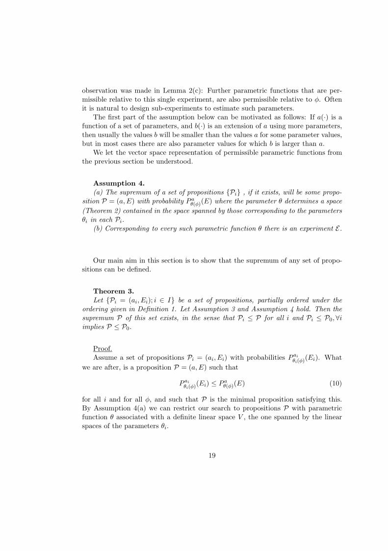
observation was made in Lemma 2(c): Further parametric functions that are per-missible relative to this single experiment, are also permissible relative to φ. Oftenit is natural to design sub-experiments to estimate such parameters.

The first part of the assumption below can be motivated as follows: If a(·) is afunction of a set of parameters, and b(·) is an extension of a using more parameters,then usually the values b will be smaller than the values a for some parameter values,but in most cases there are also parameter values for which b is larger than a.

We let the vector space representation of permissible parametric functions fromthe previous section be understood.

Assumption 4.(a) The supremum of a set of propositions {Pi} , if it exists, will be some propo-

sition P = (a,E) with probability P aθ(φ)(E) where the parameter θ determines a space(Theorem 2) contained in the space spanned by those corresponding to the parametersθi in each Pi.

(b) Corresponding to every such parametric function θ there is an experiment E.

Our main aim in this section is to show that the supremum of any set of propo-sitions can be defined.

Theorem 3.Let {Pi = (ai, Ei); i ∈ I} be a set of propositions, partially ordered under the

ordering given in Definition 1. Let Assumption 3 and Assumption 4 hold. Then thesupremum P of this set exists, in the sense that Pi ≤ P for all i and Pi ≤ P0,∀iimplies P ≤ P0.

Proof.Assume a set of propositions Pi = (ai, Ei) with probabilities P ai

θi(φ)(Ei). Whatwe are after, is a proposition P = (a,E) such that

P ai

θi(φ)(Ei) ≤ P aθ(φ)(E) (10)

for all i and for all φ, and such that P is the minimal proposition satisfying this.By Assumption 4(a) we can restrict our search to propositions P with parametricfunction θ associated with a definite linear space V , the one spanned by the linearspaces of the parameters θi.

19

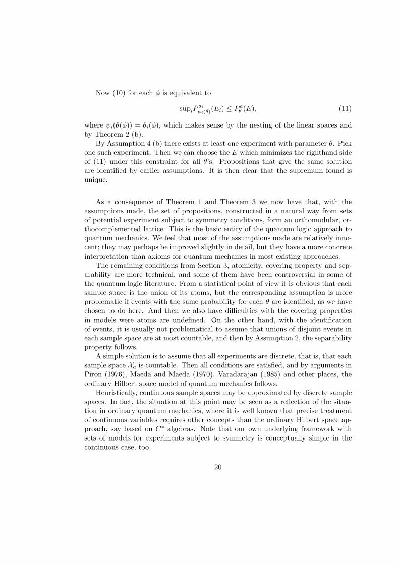
Now (10) for each φ is equivalent to

supiPai

ψi(θ)(Ei) ≤ P aθ (E), (11)

where ψi(θ(φ)) = θi(φ), which makes sense by the nesting of the linear spaces andby Theorem 2 (b).

By Assumption 4 (b) there exists at least one experiment with parameter θ. Pickone such experiment. Then we can choose the E which minimizes the righthand sideof (11) under this constraint for all θ’s. Propositions that give the same solutionare identified by earlier assumptions. It is then clear that the supremum found isunique.

As a consequence of Theorem 1 and Theorem 3 we now have that, with theassumptions made, the set of propositions, constructed in a natural way from setsof potential experiment subject to symmetry conditions, form an orthomodular, or-thocomplemented lattice. This is the basic entity of the quantum logic approach toquantum mechanics. We feel that most of the assumptions made are relatively inno-cent; they may perhaps be improved slightly in detail, but they have a more concreteinterpretation than axioms for quantum mechanics in most existing approaches.

The remaining conditions from Section 3, atomicity, covering property and sep-arability are more technical, and some of them have been controversial in some ofthe quantum logic literature. From a statistical point of view it is obvious that eachsample space is the union of its atoms, but the corresponding assumption is moreproblematic if events with the same probability for each θ are identified, as we havechosen to do here. And then we also have difficulties with the covering propertiesin models were atoms are undefined. On the other hand, with the identificationof events, it is usually not problematical to assume that unions of disjoint events ineach sample space are at most countable, and then by Assumption 2, the separabilityproperty follows.

A simple solution is to assume that all experiments are discrete, that is, that eachsample space Xa is countable. Then all conditions are satisfied, and by arguments inPiron (1976), Maeda and Maeda (1970), Varadarajan (1985) and other places, theordinary Hilbert space model of quantum mechanics follows.

Heuristically, continuous sample spaces may be approximated by discrete samplespaces. In fact, the situation at this point may be seen as a reflection of the situa-tion in ordinary quantum mechanics, where it is well known that precise treatmentof continuous variables requires other concepts than the ordinary Hilbert space ap-proach, say based on C∗ algebras. Note that our own underlying framework withsets of models for experiments subject to symmetry is conceptually simple in thecontinuous case, too.

20

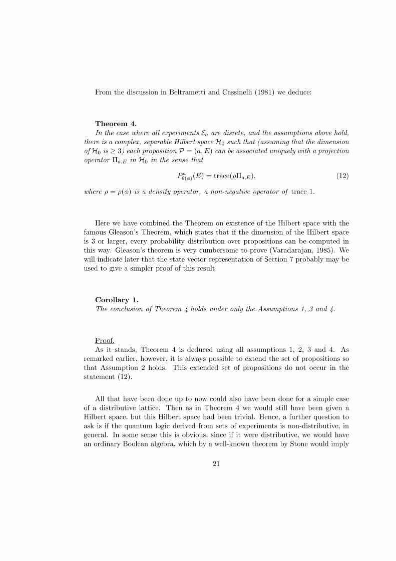
From the discussion in Beltrametti and Cassinelli (1981) we deduce:

Theorem 4.In the case where all experiments Ea are disrete, and the assumptions above hold,

there is a complex, separable Hilbert space H0 such that (assuming that the dimensionof H0 is ≥ 3) each proposition P = (a,E) can be associated uniquely with a projectionoperator Πa,E in H0 in the sense that

P aθ(φ)(E) = trace(ρΠa,E), (12)

where ρ = ρ(φ) is a density operator, a non-negative operator of trace 1.

Here we have combined the Theorem on existence of the Hilbert space with thefamous Gleason’s Theorem, which states that if the dimension of the Hilbert spaceis 3 or larger, every probability distribution over propositions can be computed inthis way. Gleason’s theorem is very cumbersome to prove (Varadarajan, 1985). Wewill indicate later that the state vector representation of Section 7 probably may beused to give a simpler proof of this result.

Corollary 1.The conclusion of Theorem 4 holds under only the Assumptions 1, 3 and 4.

Proof.As it stands, Theorem 4 is deduced using all assumptions 1, 2, 3 and 4. As

remarked earlier, however, it is always possible to extend the set of propositions sothat Assumption 2 holds. This extended set of propositions do not occur in thestatement (12).

All that have been done up to now could also have been done for a simple caseof a distributive lattice. Then as in Theorem 4 we would still have been given aHilbert space, but this Hilbert space had been trivial. Hence, a further question toask is if the quantum logic derived from sets of experiments is non-distributive, ingeneral. In some sense this is obvious, since if it were distributive, we would havean ordinary Boolean algebra, which by a well-known theorem by Stone would imply

21

that everything could be represented as one single experiment. Here is a simpleexample of non-distributivity. More complicated examples can be constructed fromthis.

Example 1.Look at two experiments Ea = (X ,F , {Pθ}) and Eb = (Y,G, {Qψ}). Let A,B ∈ F ,

A,B 6= X , but A ∪ B = X , and let C ∈ G, C 6= ∅. Assume that the twoexperiments are unrelated in the sense that θ and ψ depend on the common pa-rameter φ in disjoint parts of its range Φ. Also assume that Pθ(A) = Pθ(B) =Qψ(C) = 0 in the areas where these are independent of the parameters. Then(a,Ac) ∨ (b, Cc) is some proposition (e,D) whose probability for all φ should dom-inate max(Pθ(φ)(Ac), Qψ(φ)(Cc)). But, from the assumptions made, this maximummust be 1 for all φ. Hence (a,Ac) ∨ (b, Cc) = 1, so (a,A) ∧ (b, C) = 0. Similarly,(a,B) ∧ (b, C) = 0, so ((a,A) ∧ (b, C)) ∨ ((a,B) ∧ (b, C)) = 0. On the other hand,((a,A) ∨ (a,B)) ∧ (b, C) = (a,A ∪ B) ∧ (b, C) = 1 ∧ (b, C) = (b, C). So these threeevents do not satisfy the distributive law.

Finally, one can ask if the quantum logic derived from sets of potential experimentis wide enough to cover everything that is of interest in quantum mechanics. Ofcourse, it is very ambitious to try to give an answer to such a question, but it is anencouraging thought that virtually every attempt that can be made to verify anytheory on the quantum level has to be based on experiments. Hence it seems verydifficult to trancend beyond this frame. (However, this argument does perhaps nothold for quantum cosmology.)

9 Observables.

In Section 7 we introduced a group representation of the transformation group Gin the parameter space, and looked at some concrete interpretations of that rep-resentation in Theorem 2. The Hilbert space of Theorem 4 can in some sense beregarded as the corresponding representation of the sample space group G. Eventhough the consequences of this latter representation are discussed in all books inquantum mechanics, we will come with some remarks on it here.

Since we have assumed that all sample spaces Xa are discrete (this is not necessaryfor our basic model, but convenient for the Hilbert space representation), we mightas well assume that Xa = {1, 2, . . .} for each a. The σ-algebra is then the obvious one,

22

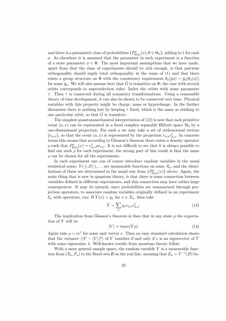
and there is a parametric class of probabilities {P aθ(φ)(x); θ ∈ Θa}, adding to 1 for eacha. As elsewhere it is assumed that the parameter in each experiment is a functionof a state parameter φ ∈ Φ. The most important assumptions that we have made,apart from that the class of experiments should be rich enough, is that pairwiseorthogonality should imply total orthogonality in the sense of (1) and that thereexists a group structure on Φ with the consistency requirement θa(gφ) = ga(θa(φ))for some ga. We will also assume here that G is transitive on Φ; the case with severalorbits corresponds to superselection rules: Index the orbits with some parameterτ . Then τ is conserved during all symmetry transformations. Using a reasonabletheory of time development, it can also be shown to be conserved over time. Physicalvariables with this property might be charge, mass or hypercharge. In the furtherdiscussion there is nothing lost by keeping τ fixed, which is the same as sticking toone particular orbit, so that G is transitive.

The simplest quantummechanical interpretation of (12) is now that each primitiveevent (a, x) can be represented in a fixed complex separable Hilbert space H0 by aone-dimensional projection: For each a we may take a set of orthonormal vectors{ea,x}, so that the event (a, x) is represented by the projection ea,xe

†a,x. In concrete

terms this means that according to Gleason’s theorem there exists a density operatorρ such that P aθ(φ)(x) = e†a,xρea,x. It is not difficult to see that it is always possible tofind one such ρ for each experiment; the strong part of this result is that the sameρ can be chosen for all the experiments.

In each experiment one can of course introduce random variables in the usualstatistical sense: Y (·), Z(·), . . . are measurable functions on some Xa, and the distri-butions of these are determined in the usual way from {P aθ(φ)(x)} above. Again, themain thing that is new in quantum theory, is that there is some connection betweenvariables defined in different experiments, and this connection may have rather largeconsequences. It may be natural, since probabilities are summarized through pro-jection operators, to associate random variables originally defined in an experimentEa with operators, too: If Y (x) = yx for x ∈ Xa, then take

Y =∑x

yxea,xe†a,x. (13)

The implication from Gleason’s theorem is then that in any state ρ the expecta-tion of Y will be

〈Y 〉 = trace(Y ρ). (14)

Again take ρ = ee† for some unit vector e. Then an easy standard calculation showsthat the variance 〈(Y − 〈Y 〉)2〉 of Y vanishes if and only if e is an eigenvector of Ywith some eigenvalue λ. Well-known results from quantum theory follow.

With a more general sample space, the random variable Y is a measurable func-tion from (Xa,Fa) to the Borel sets B on the real line, meaning that Ea = Y −1(B) be-

23

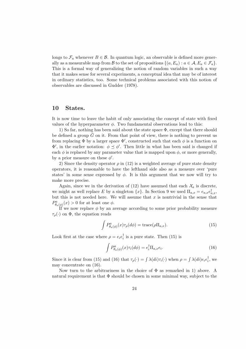
longs to Fa whenever B ∈ B. In quantum logic, an observable is defined more gener-ally as a measurable map from B to the set of propositions {(a,Ea) : a ∈ A, Ea ∈ Fa}.This is a formal way of generalizing the notion of random variables in such a waythat it makes sense for several experiments, a conceptual idea that may be of interestin ordinary statistics, too. Some technical problems associated with this notion ofobservables are discussed in Gudder (1978).

10 States.

It is now time to leave the habit of only associating the concept of state with fixedvalues of the hyperparameter φ. Two fundamental observations lead to this:

1) So far, nothing has been said about the state space Φ, except that there shouldbe defined a group G on it. From that point of view, there is nothing to prevent usfrom replacing Φ by a larger space Φ′, constructed such that each φ is a function onΦ′, in the earlier notation: φ � φ′. Then little in what has been said is changed ifeach φ is replaced by any parameter value that is mapped upon φ, or more generally,by a prior measure on these φ′.

2) Since the density operator ρ in (12) is a weighted average of pure state densityoperators, it is reasonable to have the lefthand side also as a measure over ‘purestates’ in some sense expressed by φ. It is this argument that we now will try tomake more precise.

Again, since we in the derivation of (12) have assumed that each Xa is discrete,we might as well replace E by a singleton {x}. In Section 9 we used Πa,x = ea,xe

†a,x,

but this is not needed here. We will assume that x is nontrivial in the sense thatP aθa(φ)(x) > 0 for at least one φ.

If we now replace φ by an average according to some prior probability measureτρ(·) on Φ, the equation reads∫

P aθa(φ)(x)τρ(dφ) = trace(ρΠa,x). (15)

Look first at the case where ρ = eie†i is a pure state. Then (15) is∫

P aθa(φ)(x)τi(dφ) = e†iΠa,xei. (16)

Since it is clear from (15) and (16) that τρ(·) =∫λ(di)τi(·) when ρ =

∫λ(di)eie

†i , we

may concentrate on (16).Now turn to the arbitrariness in the choice of Φ as remarked in 1) above. A

natural requirement is that Φ should be chosen in some minimal way, subject to the

24

requirement that it should serve as a hyperparameter space for all the experimentsin questions. In fact the concept of minimality can be made completely precise wehave the ordering � of parametric functions.

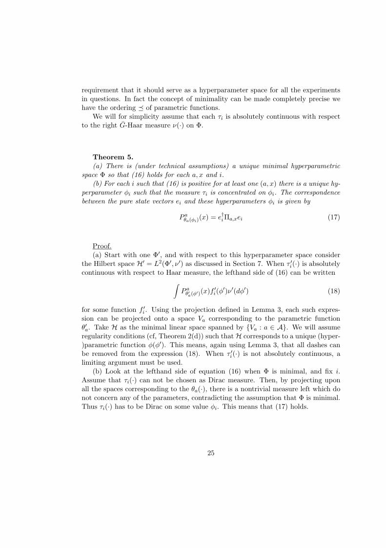
We will for simplicity assume that each τi is absolutely continuous with respectto the right G-Haar measure ν(·) on Φ.

Theorem 5.(a) There is (under technical assumptions) a unique minimal hyperparametric

space Φ so that (16) holds for each a, x and i.(b) For each i such that (16) is positive for at least one (a, x) there is a unique hy-

perparameter φi such that the measure τi is concentrated on φi. The correspondencebetween the pure state vectors ei and these hyperparameters φi is given by

P aθa(φi)(x) = e†iΠa,xei (17)

Proof.(a) Start with one Φ′, and with respect to this hyperparameter space consider

the Hilbert space H′ = L2(Φ′, ν ′) as discussed in Section 7. When τ ′i(·) is absolutelycontinuous with respect to Haar measure, the lefthand side of (16) can be written∫

P aθ′a(φ′)(x)f′i(φ

′)ν ′(dφ′) (18)

for some function f ′i . Using the projection defined in Lemma 3, each such expres-sion can be projected onto a space Va corresponding to the parametric functionθ′a. Take H as the minimal linear space spanned by {Va : a ∈ A}. We will assumeregularity conditions (cf, Theorem 2(d)) such that H corresponds to a unique (hyper-)parametric function φ(φ′). This means, again using Lemma 3, that all dashes canbe removed from the expression (18). When τ ′i(·) is not absolutely continuous, alimiting argument must be used.

(b) Look at the lefthand side of equation (16) when Φ is minimal, and fix i.Assume that τi(·) can not be chosen as Dirac measure. Then, by projecting uponall the spaces corresponding to the θa(·), there is a nontrivial measure left which donot concern any of the parameters, contradicting the assumption that Φ is minimal.Thus τi(·) has to be Dirac on some value φi. This means that (17) holds.

25

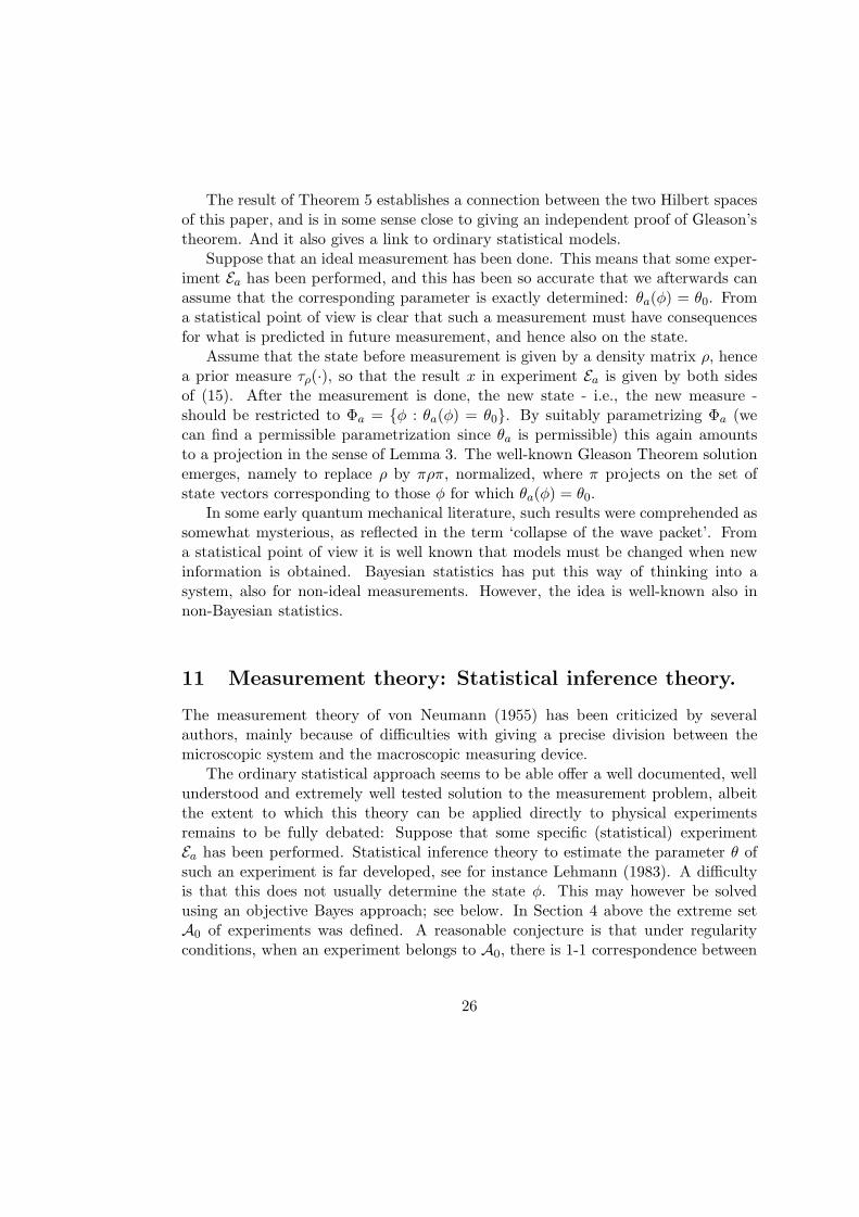
The result of Theorem 5 establishes a connection between the two Hilbert spacesof this paper, and is in some sense close to giving an independent proof of Gleason’stheorem. And it also gives a link to ordinary statistical models.

Suppose that an ideal measurement has been done. This means that some exper-iment Ea has been performed, and this has been so accurate that we afterwards canassume that the corresponding parameter is exactly determined: θa(φ) = θ0. Froma statistical point of view is clear that such a measurement must have consequencesfor what is predicted in future measurement, and hence also on the state.

Assume that the state before measurement is given by a density matrix ρ, hencea prior measure τρ(·), so that the result x in experiment Ea is given by both sidesof (15). After the measurement is done, the new state - i.e., the new measure -should be restricted to Φa = {φ : θa(φ) = θ0}. By suitably parametrizing Φa (wecan find a permissible parametrization since θa is permissible) this again amountsto a projection in the sense of Lemma 3. The well-known Gleason Theorem solutionemerges, namely to replace ρ by πρπ, normalized, where π projects on the set ofstate vectors corresponding to those φ for which θa(φ) = θ0.

In some early quantum mechanical literature, such results were comprehended assomewhat mysterious, as reflected in the term ‘collapse of the wave packet’. Froma statistical point of view it is well known that models must be changed when newinformation is obtained. Bayesian statistics has put this way of thinking into asystem, also for non-ideal measurements. However, the idea is well-known also innon-Bayesian statistics.

11 Measurement theory: Statistical inference theory.

The measurement theory of von Neumann (1955) has been criticized by severalauthors, mainly because of difficulties with giving a precise division between themicroscopic system and the macroscopic measuring device.

The ordinary statistical approach seems to be able offer a well documented, wellunderstood and extremely well tested solution to the measurement problem, albeitthe extent to which this theory can be applied directly to physical experimentsremains to be fully debated: Suppose that some specific (statistical) experimentEa has been performed. Statistical inference theory to estimate the parameter θ ofsuch an experiment is far developed, see for instance Lehmann (1983). A difficultyis that this does not usually determine the state φ. This may however be solvedusing an objective Bayes approach; see below. In Section 4 above the extreme setA0 of experiments was defined. A reasonable conjecture is that under regularityconditions, when an experiment belongs to A0, there is 1-1 correspondence between

26

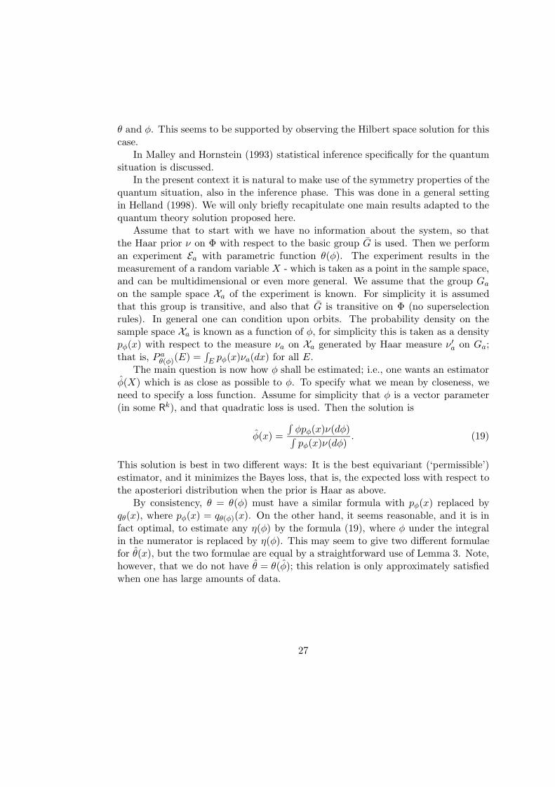
θ and φ. This seems to be supported by observing the Hilbert space solution for thiscase.

In Malley and Hornstein (1993) statistical inference specifically for the quantumsituation is discussed.

In the present context it is natural to make use of the symmetry properties of thequantum situation, also in the inference phase. This was done in a general settingin Helland (1998). We will only briefly recapitulate one main results adapted to thequantum theory solution proposed here.

Assume that to start with we have no information about the system, so thatthe Haar prior ν on Φ with respect to the basic group G is used. Then we performan experiment Ea with parametric function θ(φ). The experiment results in themeasurement of a random variable X - which is taken as a point in the sample space,and can be multidimensional or even more general. We assume that the group Gaon the sample space Xa of the experiment is known. For simplicity it is assumedthat this group is transitive, and also that G is transitive on Φ (no superselectionrules). In general one can condition upon orbits. The probability density on thesample space Xa is known as a function of φ, for simplicity this is taken as a densitypφ(x) with respect to the measure νa on Xa generated by Haar measure ν ′a on Ga;that is, P aθ(φ)(E) =

∫E pφ(x)νa(dx) for all E.

The main question is now how φ shall be estimated; i.e., one wants an estimatorφ(X) which is as close as possible to φ. To specify what we mean by closeness, weneed to specify a loss function. Assume for simplicity that φ is a vector parameter(in some Rk), and that quadratic loss is used. Then the solution is

φ(x) =∫φpφ(x)ν(dφ)∫pφ(x)ν(dφ)

. (19)

This solution is best in two different ways: It is the best equivariant (‘permissible’)estimator, and it minimizes the Bayes loss, that is, the expected loss with respect tothe aposteriori distribution when the prior is Haar as above.

By consistency, θ = θ(φ) must have a similar formula with pφ(x) replaced byqθ(x), where pφ(x) = qθ(φ)(x). On the other hand, it seems reasonable, and it is infact optimal, to estimate any η(φ) by the formula (19), where φ under the integralin the numerator is replaced by η(φ). This may seem to give two different formulaefor θ(x), but the two formulae are equal by a straightforward use of Lemma 3. Note,however, that we do not have θ = θ(φ); this relation is only approximately satisfiedwhen one has large amounts of data.

27

12 Time evolution and the role of Planck’s constant.

So far the description has been static; we will now try briefly to take time develop-ment into account. The point of departure is that we have defined the state of thesystem as some parameter φ in some space Φ. In practice this state can develop withtime in many different ways. A simple and physically plausible assumption is thatthere is a continuous group K acting on Φ such that φ after time t changes to ktφ,where kt ∈ K.

In Section 7 we discussed a unitary representation of the symmetry group G ofΦ on a Hilbert space H. Assume that one can find a unitary representation of Kalso on H. Since K is a continuous group, a well-known theorem by Stone impliesthat the representation then must be of the form

U(t) = eiAt

for some selfadjoint operator A, perhaps after rescaling time. As is demonstrated inseveral books, taking A = −H/h here, where h is Planck’s constant and H is theHamiltonian, leads to the Schrodinger equation.

This is the first time that Planck’s constant appears in this paper, a rather signif-icant observation. Everything that has been said on stochastical models, and mostof what we have said about symmetry, apply also to large-scale problems. Planck’sconstant appears only when we meet the following fact, most recently commented onby Alfsen and Schultz (1998): Physical variables play a dual role, as observables andas generators of transformation groups. It is when observators are used as generatorsof groups the proportionality constant h occurs. One example is the Hamiltonianand the Schrodinger equation, another example is the translation group in some di-rection, say the x-axis, whose unitary representation is of the form exp(ipx/h), withpx being the momentum in the x-direction.

13 A large scale example.

Most socalled paradoxes of quantum mechanics seem to disappear in the statisticalsetting described here. Take the Einstein-Podolsky-Rosen paradox for example (inthe form proposed by David Bohm): A composite particle with spin 0 disintegratesinto two single particles, whose spin components in any direction then necessarilyadd to 0, hence are opposite. Sometimes the fact that an observation of one parti-cle implies the knowledge of the spin component of the other particle in the samedirection, is taken as some action at a distance. One point is that the observer of

28

the first particle is free to choose the direction in which he wants to measure. In thelanguage of the present paper this observer chooses one particular experiment. Noparadox appears when we have a statistical interpretation of experiments in mind.

The following macroscopic example seems to be fairly similar: An organizer Osends two envelopes I and II to each of two persons A and B, situated at differentplaces. In envelope I he has the choice between a red card or a black card; eitherred to A or black to B or the opposite. In envelope II he has the choice betweena card with the letter 1 or a card with the letter 2; either 1 to A and 2 to B orthe opposite. Now O for simplicity chooses to have probability 1/2 for red to A inenvelope I, and he also chooses probability 1/2 for 1 to A in envelope II. However,he may insist that there should be some correlation γ between the two envelopes toA, for instance defined by

P (red, 1) =14(1 + γ),

where −1 ≤ γ ≤ 1. Correlation at B, defined in the same way, will then necessarilyalso be γ.

The initial state of the system is then determined, since we know the probabilitydistribution of any experiment that A and B could choose to do. To make completelyconcrete that some randomness is involved, one can imagine several independentpairs (A1, B1), . . . , (An, Bn), all in the same state, that is, under the same jointprobability distribution generated by O.

Imagine now that the following happens: A is given the order that he shouldopen one and only one envelope. Once he has opened one envelope, the other oneis destroyed (by some mechanism which is irrelevant here). A is therefore giventhe choice between two noncompatible experiment, exactly the situation discussedin this paper. If he opens envelope I and finds a red card, he can make one set ofpredictions concerning the content of B’s two envelopes; if he opens envelope II andsees the number 2, he can make another set of predictions, etc.. The situation is atleast in some sense similar to the EPR-experiment. There is no action at a distance,only predictions conditioned on different information.

As the experiment is described above, however, the well known inequalities of Bell(1966) will always be satisfied, since the knowledge posessed by O can be regardedas a hidden variable. But the example can be extended in several directions, thuspossibly making it more equal to its quantummechanical counterparts.

The following concept is of interest in general, and specifically in this example:Pick a set A1 of potential experiments. Then the set {(a, θa) : a ∈ A1} may be calledpermissible if there is a group G1 on A1 such that (i) g1a ∈ A1 whenever a ∈ A1 andg1 ∈ G1, and (ii) (g1a, θg1a(gφ)) is a function of (a, θa(φ)) for all choices of g1, g. Thisis equivalent to permissibility of the parameter in a compound experiment, where φis augmented by the ‘parameter’ a, and the group of this new φ is given by {(g1, g)}.

29

In the present example, the 3 transformations corresponding to Pθ(r) → Pθ(b)(envelope I), Pθ(1) → Pθ(2) (envelope II) and I → II (change envolope) constitutesuch a structure. The smallest homomorphic image of S4 (the permutation group of4 elements) which supports this structure, is S3, which is noncommutative and hasan interesting 2-dimensional irreducible representation.

Several concepts of this paper may be illustrated on this simple example, ifnecessary by using the structure just described. Alternatively, the example couldhave been made more complicated to start with, so that each experiment supported agroup with a nontrivial irreducible representation. These (not quite trivial) exerciseswill be left to the interested reader. One extension will be discussed in Helland(1999).

14 Discussion.

Throughout this paper we have stated some assumptions; in addition there are sev-eral implicit assumptions of more technical/ mathematical type. Though most ofthese assumptions are rather plausible, we are not completely sure that all of themwill be satisfied in all details in a future hypothetical theory. Their main functionhere have been to pave the way to ordinary quantum mechanics from what is ourbasic framework: Set of models for experiments with a common state space, subjectto some symmetry group.

Our conceptual framework works both for continuous and for discrete variables,and, apart from the discussion of time evolution, there is not much non-relativisticabout it. A very interesting - but probably not trivial - question is therefore towhat extent it can be developed further in a relativistic setting, perhaps even withthe kind of symmetry groups that are natural to think of in the contexts of generalrelativity.

Of some interest in this connection are the views expressed by Dirac (1978):He wanted relativistic quantum mechanics to take another direction, and explicitlymentioned group representations of the Poincare group as a clue to this direction.

In the same paper, Paul Dirac expressed the following opinion: ‘One should keepthe need for a sound mathematical basis dominating one’s search for a new theory,Any physical or philosophical idea that one has must be adjusted to the mathematics.Not the other way around.’

I strongly agree with Dirac that any fundamental physical theory should have asound mathematical basis. In fact, much of the motivation behind the present paperhas been to find just that. However, every mathematical theory building must bebased on a set of axioms. It may well be that the axioms found by mathematicians

30

using aesthetic or quasi-logical criteria are among the right ones to serve as a basisfor a physical theory, but these criteria alone often leaves one with too much arbi-trariness. In fact, and unfortunately, much formalistic theory has been the resultof only taking such points of departure. To find the basis for a new theory, onemust endeavor to look in all directions, draw upon all sources whether they relateto common sense, experience, mathematics, philosophy or large scale physics.

This implies extremely difficult requirements on the developer of theories, andintuitive reasoning and even imprecise arguments seem to be unavoidable at inter-mediate stages of the development. Having said that, however, at the final stagemathematical rigor should be imperative.

It can be inferred from the ideas of this paper that much of what has beensaid about modelling in microcosmos also can be transferred to macrocosmos. Infact, large scale examples showing quantum mechanical behavior has recently beendemonstrated in the physical literature (Aerts, 1996). As indicated above: Severalexamples of this type can be constructed.

Having stressed the similarities between models of quantum theory and those ofstatistics in this paper, it should also of course be underlined that there are basicdifferences. In statistics the parameters are always regarded as unknown and subjectto inference; in quantum physics the states/ parameters can often be regarded asknown. Also, the rich set of symmetries that is typical for all applications of quantumtheory, seldom find their counterpart, at least not to a similar degree, in large scalestatistics.

Nevertheless, even though it is not a main issue here, it should be mentioned thatsome of the ideas behind this paper also seem to have impact also for issues discussedin ordinary statistical science. The question of how to condition statistical modelsgives another meaning to the label ‘a’ in Ea = (Xa,Fa, {P aθ ; θ ∈ Θa}) (Helland,1995, and references there). The link between this issue and quantum mechanicswas suggested already by Barndorff-Nielsen (1995).

In this paper, and in most statistical papers, a mathematical structure like Eaabove is connected to a real, physical or otherwise, experiment. But in addition,since {P aθ } is included in the structure, it can be used to denote different models forthe same real experiment. This idea together with the symmetry discussion of thepresent paper can in fact be used to discuss model reduction in statistics. We hopeto develop these ideas further elsewhere.

31

References.

Aerts, S. (1996). Conditional probabilities with a quantal and a Kolmogorovianlimit. Int. J. Theoret. Phys. 35, 2245-2261.

Alfsen, E.M. and F.W. Schultz (1998). Orientation in operator algebras. Proc.Natl. Acad. Sci. USA 95, 6596-6601.

Aspect, A., J. Dalibard and G. Roger (1982). Experimental test of Bell inequal-ities using time-varying analysers. Phys. Rev. Lett. 49, 1804ff.

Barndorff-Nielsen, O.E. (1995). Diversity of evidence and Birnbaum’s theorem.Scand. J. Statist. 22, 513-522.

Barut, A.O. and R. Raczka (1977). Theory of Group Representations and Appli-cations. Polish Scientific Publishers, Warszawa.

Bell, J.S. (1966) On the problem of hidden variables in quantum mechanics. Rev.Mod. Phys. 38, 447-452.

Beltrametti, E.G. and G. Cassinelli (1981). The Logic of Quantum Mechanics.Addison-Wesley, London.

Beran, L. (1985). Orthomodular Lattices. Algebraic Approach. D. Reidel Pub-lishing Company, Dordrecht.

Berger, J. O. (1985). Statistical Decision Theory and Bayesian Analysis. Springer-Verlag, New York.

Bohr, A. and O. Ulfbeck (1995). Primary manifestation of symmetry. Origin ofquantal indeterminacy. Reviews of Modern Physics 67, 1-35.

Cox, D.R. and D.V. Hinkley (1974). Theoretical Statistics. Chapman and Hall,London.

Dirac, P.A.M. (1978). The mathematical foundations of quantum theory. In:Marlow, A.R. [Ed.] Mathematical Foundations of Quantum Theory. Academic Press,New York.

Dunford, N. and J.T. Schwartz (1958). Linear Operators. Part I: General The-ory. Interscience Publishers, New York.

Feynman, R.P. (1951). The concept of probability in quantum mechanics. Sec-ond Berkeley Symposium on Mathematical Statistixs and probability. University ofCalifornia Press, Berkeley, California.

Gudder, S.P. (1978). Some unsolved problems in quantum logic. In: Marlow,A.R. [Ed.] Mathematical Foundations of Quantum Theory. Academic Press, NewYork.

Hamermesh, M. (1962). Group Theory and its Applications to Physical Problems.Addison-Wesley, Reading, Massachusetts.

Helland, I.S. (1995). Simple counterexamples against the conditionality principle.Amer. Statist. 49, 351-356. Correction/ discussion: Amer. Statist. 50, 382-386.

32

Helland, I.S. (1998). Statistical inference under a fixed symmetry group. Sta-tistical Research Report No. 7, Department of Mathematics, University of Oslo.

Helland, I.S. (1999). Relation between quantum theory and symmetry structuresin a parameter space for statistical experiments. Preprint.

Kalmbach, G. (1983). Orthomodular Lattices. Academic Press, London.Lehmann, E.L. (1983). Theory of Point Estimation. Springer-Verlag, New York.Mackey, G.W. (1963). The Mathematical Foundations of Quantum Mechanics.

W.A. Benjamin, New York.Maczynski, M.J. (1973). The orthogonality postulate in axiomatic quantum me-

chanics. Int. Journ. Theor. Physics 8, 353-360.Maeda, F. and S. Maeda (1970). Theory of Symmetric Lattices. Springer-Verlag,

Berlin.Malley, J.D. and J. Hornstein (1993). Quantum statistical inference. Statistical

Science 8, 433-457.Meyer, P.-A. (1993). Quantum Probability for Probabilists. Springer-Verlag,

Berlin.Nachbin, L. (1965). The Haar Integral, Van Nostrand, Princeton, N.J.von Neumann, J. (1955). Mathematical Foundations of Quantum Mechanics.

Princeton University Press, Princeton.Piron, C. (1976). Foundation of Quantum Physics. W.A. Benjamin. Inc., Lon-

don.Varadarajan, V.S. (1985). Geometry of Quantum Theory. Springer, New York.

33