Quantum Informationwith

Continuous Variables

Klaus Mølmer

University of Aarhus, Denmark

Supported by the European Union and

The US Office of Naval Reseach

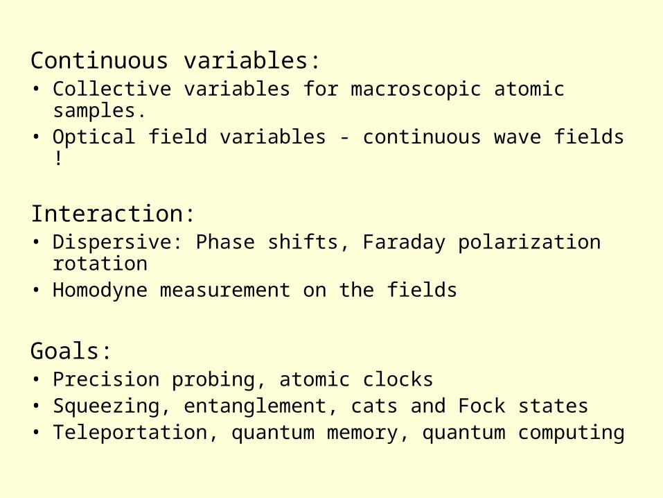
Continuous variables:• Collective variables for macroscopic atomic samples.• Optical field variables - continuous wave fields !

Interaction:• Dispersive: Phase shifts, Faraday polarization rotation• Homodyne measurement on the fields

Goals:• Precision probing, atomic clocks• Squeezing, entanglement, cats and Fock states• Teleportation, quantum memory, quantum computing

Outline

• Continuous variable physical systems• Gaussian state formalism• Three applications:

– Squeezing and entanglement– Magnetometry – Photons from fields

• Outlook

Continuous variables for two-level atoms

• Many atoms in (|↑>+|↓>)/√2 <Jx>=Nat/2,

<Jy>=<Jz>=0

Var(Jy)Var(Jz) = |<Jx>|2/4 binomial noise

(M.U.S.).

let pat = Jz/√<Jx>, xat = Jy/ /√<Jx>, [xat,pat]=i

harmonic oscillator degrees of freedom.

”Ground state” is Gaussian in xat,pa

Also without 100 % optical pumping!

|↓>|↑>

Normally,

ρ1 atom is quantum.

Here, collective

pat, xat, are our

Quantum Variables !

Continuous variables for polarized light

x-polarized light has <Sx> = Nph/2, <Sy> = <Sz> = 0.

let pph = Sz/√<Sx>, xph = Sy/ /√<Sx>, [xph,pph]=i

harmonic oscillator ground state, Gaussian in xph,pph

Interaction• Dispersive atom-light interaction:

σ+ (σ-) light is phase shifted by |↑> (|↓>) atoms

Faraday polarization rotation, proportional to <Jz>

Hint = g SzJz = к pat pph

|↓>|↑>

Update of atomic state due to interaction with a light pulse

Hint = g SzJz = к pph pat

pph unchanged

xph xph + к t pat

xph is measured:

we learn about pat, we ”unlearn” about xat

pat unchanged

xat xat + к t pph

Gaussian states

State characterized by• vector of (x’s and p’s) with mean values m• γ = matrix of covariances, γij= 2<(yi-mi)(yj-mj)>

P(y) = N exp(-(y-m)T γ-1 (y-m))

Gaussian states (m and γ) transform under xx, xp and pp interactions (linear optics, squeezing), decay and losses.

Gaussian states (m and γ) transform under measurements of x’s and p’s (Stern-Gerlach and homodyne detection).

Quantum case:

Heisenberg uncertainty limit on γ

Update of Gaussian atomic state due to interaction with a light pulse

)0

0(

IA

)0

0´´(

IA

)´

(FFA

AFA

Loss of light:

γph(1-ε)γph +ε II

Atomic decay:

γat(1-ηΔt)γat +2(ηΔt) II

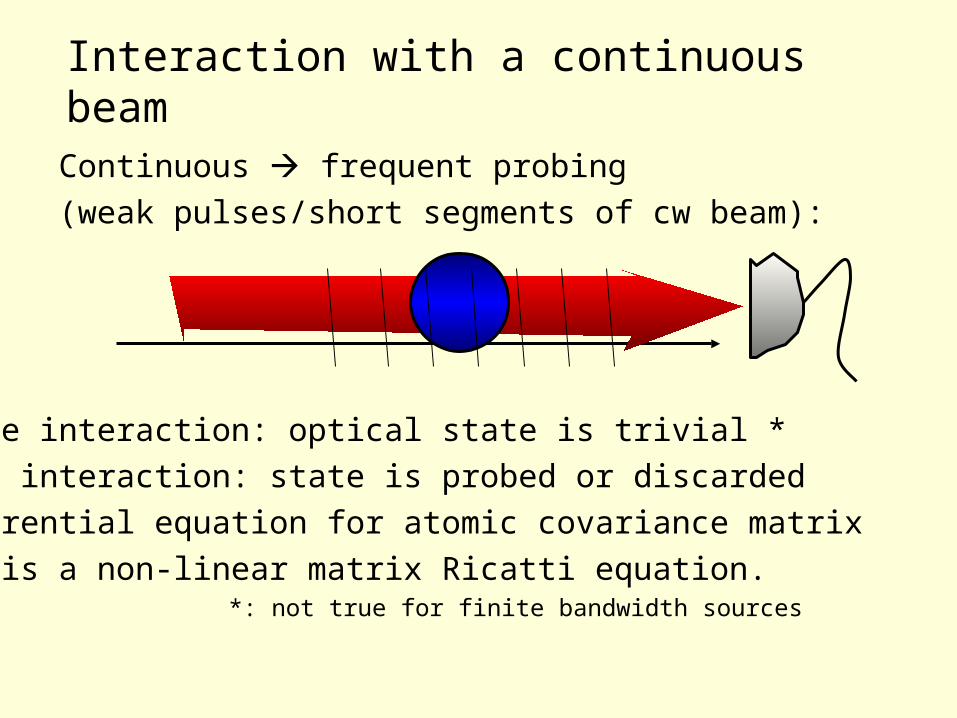
Interaction with a continuous beam

Continuous frequent probing

(weak pulses/short segments of cw beam):

Before interaction: optical state is trivial *

After interaction: state is probed or discarded

Differential equation for atomic covariance matrix

This is a non-linear matrix Ricatti equation.*: not true for finite bandwidth sources

Application 1:

Squeezing and Entanglement

Atomic spin squeezing due to optical probingL. B. Madsen and K.M., Phys. Rev. A 70, 052324 (2004)

For the simple atom-light example (binomial distribution):

)22/(1)()(2)( 222 tpVarpVarpVardt

datatat

Entanglement of two gases by optical probing : Duan, Cirac, Zoller, Polzik

Measure (x1+x2) and (p1-p2)

Entanglement and The Swineherd (Hans Christian Andersen 1805-1875)

” … when one put a finger into the steam rising from the pot, one could at once smell what meals they were preparing on every fire in the whole town”

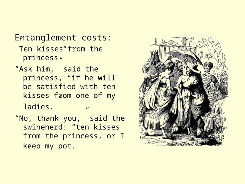
Entanglement costs:”Ten kisses from the princess”

“Ask him,” said the princess, “if he will be satisfied with ten kisses from one of my

ladies.” “No, thank you,” said the

swineherd: “ten kisses from the princess, or I keep my pot.”

How much entanglement can be generated over a lossy optical transmission lines ?

Ans.: ”Any amount, with use of repeaters and distillation.”

What is the best possible entanglement, obtained with Gaussian operations ? (Distillation forbidden).

Does the no-distillation theorem put an ultimate limit to the entanglement that we can squeeze into a single pair of distant oscillator-like systems ?

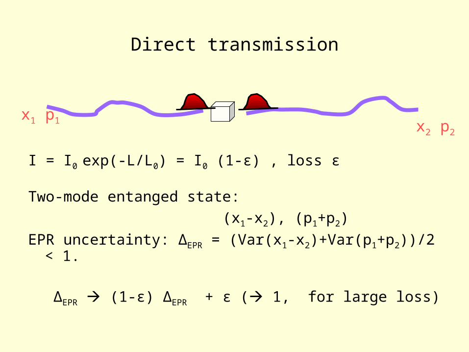
Direct transmission

I = I0 exp(-L/L0) = I0 (1-ε) , loss ε

Two-mode entanged state:

(x1-x2), (p1+p2)

EPR uncertainty: ΔEPR = (Var(x1-x2)+Var(p1+p2))/2 < 1.

ΔEPR (1-ε) ΔEPR + ε ( 1, for large loss)

x1 p1 x2 p2

Entanglement of two gases, GEoF

Polarisation rotation

Polarisation rotation

loss

Does the read-outteach us moreabout gas 1 or 2 ?

Faraday rotation with x-polarized beamH = κ1p p1 + κ2p’ p2

= κ√(1-ε) p’ (p1+p2) - κ√ε pvacp1

Atomic entanglement by probing is a bad idea !

Transmitted beams

Optically probed atoms

Finite optical squeezing

NOT

A most surprising result:Lars B. Madsen and K.M., to be published

Finite entanglement, N=1/3 for arbitrary loss:

Teleportation fidelity, F = 1/(1+N) = 75 %

for unknown coherent state.

Probed atoms (symmetric)

Infinitely squeezed light Probed atoms (one way)

with squeezed light

with anti-squeezed light

squeezing: 0.1, 10

Application 2:

Quantum Metrology

Metrology with a quantum probe

Quantum system

observer

Classical quantity

A side remark

For a quantum physicist, it is natural to think of the time evolution of the state as dynamical evolution of the physical state of the system, e.g., as the wave function is getting narrow, ”the particle localizes physically”.

According to the Copenhagen interpretation, however, the wave function/density matrix/Wigner function is not the state of the system, but rather a representation of our knowledge about the system. When we measure, we learn something.

Complete* relationship with classical theory for the estimation of a gaussian variable under noisy measurements (Riccati).

(*: but recall commutators and Heisenberg’s uncertainty relation)

Probing of a classical magnetic field (K.M & L. B. Madsen,Phys. Rev. A 70, 052102 (2004) )

P(random signal | B) P(B | signal)

Our SIMPLE approach: Treat atoms AND light AND B field by a joint Gaussian probabilityCovariance matrix for (B,xat,pat,xph,pph).Analytical solution (no noise):

Long times: ΔB~ 1/(Nat t3/2) • Independent of ΔB0

• not as 1/√Nat ,1/√t

Estimate a time dependent (noisy) magnetic fieldVivi Petersen and K.M. to be published

Noisy field

Estimator (mean of Gaussian)

Correct estimator for the current value of B(t) !(See also Mabuchi et al.)

”Gaussian hindsight”

Noisy field

Estimator (mean of Gaussian)

1. 0.02 ms delay, minimizes

2. Temporal convolution

3. Gaussian distribution for (B(t1),B(t2),.. B(tn)

measurements now, update the past.

Noisy field

Estimator (mean of Gaussian)

”Get wiser in 0.02 msec”

”If I knew then, what I know now”

Application 3:

Leaving the Gaussian states

Photons from fields.

Leaving the Gaussian states

Gaussian states do not encode qubits

(two coherent states may be almost orthogonal,

but their superposition is not a Gaussian)

Gaussian states cannot be distilled (purified)

Photons from fields

Field or photon description of light?Single mode: state and operator pictures equivalent.

Continuous beams, multi-mode:

Expansion on number states practically impossible.

Field picture useful: mean values, correlation functions.

Conditioned dynamics, collapses in Heisenberg picture?

From many to two modes:

OPO output:

Chose trigger and output modes:

Wigner function of four real variables:

(Gaussian, prior to click)

Click event (photodetection theory):

ρ a1ρa1+

Wigner function transformation:

and then trace over mode 1

Gaussian

Gaussian times a poynomial

Results:(K.M., quant-pt/0602202, today)

Weak OPO

n=1 Fock state

Strong OPO

Schrödinger kitten

75 % detection

Experiments (Grangier group) J. Wenger et al, PRL 92, 153601 (2004):

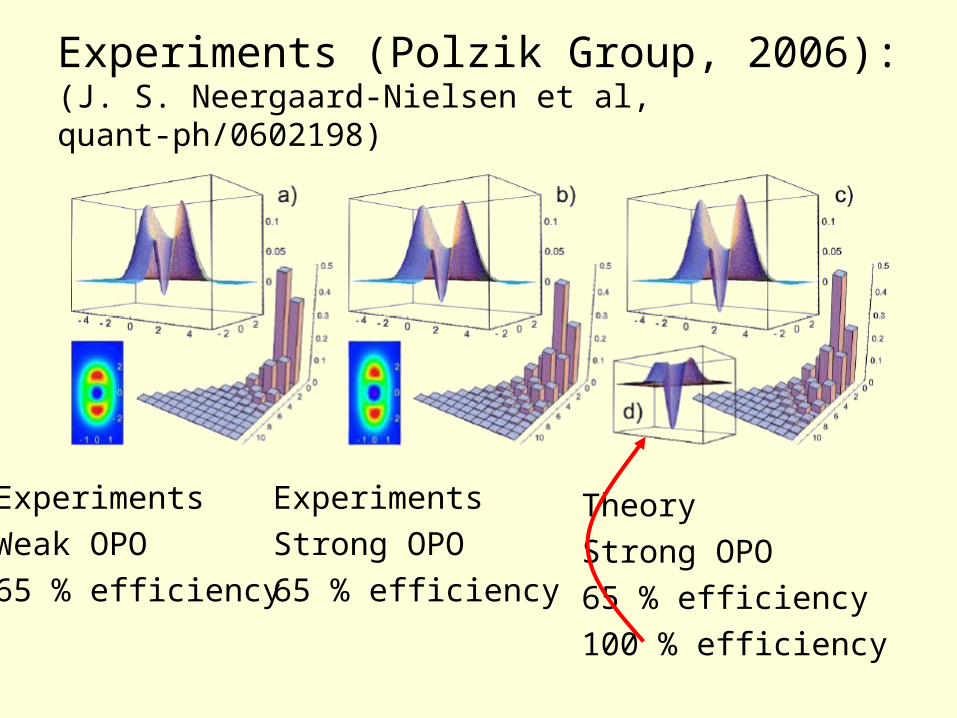
Experiments (Polzik Group, 2006):(J. S. Neergaard-Nielsen et al, quant-ph/0602198)

Experiments

Strong OPO

65 % efficiency

Experiments

Weak OPO

65 % efficiency

Theory

Strong OPO

65 % efficiency

100 % efficiency

Conclusion/outlook,

• Many atoms and many photons are ”easy experiments” (classical fields, homodyne detection)

• Many atoms and many photons is ”easy theory” (readily generalized at low cost to more samples/fields)

• Gaussian states: squeezing, entanglement, … and also: finite bandwidth sources, finite bandwidth detection

• Gaussian states unify quantum and classical variables: classical B-field + atoms + light probe

other observables: interferometry, … .• First step to non-Gaussian states, discrete qubits,

Schrödinger Cats, … .