Quantum Information Chapter 10. Quantum Shannon … · Quantum Information Chapter 10. Quantum...
119
Quantum Information Chapter 10. Quantum Shannon Theory John Preskill Institute for Quantum Information and Matter California Institute of Technology Updated June 2016 For further updates and additional chapters, see: http://www.theory.caltech.edu/people/preskill/ph219/ Please send corrections to [email protected]
Transcript of Quantum Information Chapter 10. Quantum Shannon … · Quantum Information Chapter 10. Quantum...

Quantum Information
Chapter 10. Quantum Shannon Theory
John PreskillInstitute for Quantum Information and Matter
California Institute of Technology
Updated June 2016
For further updates and additional chapters, see:http://www.theory.caltech.edu/people/preskill/ph219/
Please send corrections to [email protected]

Contents
10 Quantum Shannon Theory 110.1 Shannon for Dummies 2
10.1.1 Shannon entropy and data compression 210.1.2 Joint typicality, conditional entropy, and mutual infor-
mation 610.1.3 Distributed source coding 810.1.4 The noisy channel coding theorem 9
10.2 Von Neumann Entropy 1610.2.1 Mathematical properties of H(ρ) 1810.2.2 Mixing, measurement, and entropy 2010.2.3 Strong subadditivity 2110.2.4 Monotonicity of mutual information 2310.2.5 Entropy and thermodynamics 2410.2.6 Bekenstein’s entropy bound. 2610.2.7 Entropic uncertainty relations 27
10.3 Quantum Source Coding 3010.3.1 Quantum compression: an example 3110.3.2 Schumacher compression in general 34
10.4 Entanglement Concentration and Dilution 3810.5 Quantifying Mixed-State Entanglement 45
10.5.1 Asymptotic irreversibility under LOCC 4510.5.2 Squashed entanglement 4710.5.3 Entanglement monogamy 48
10.6 Accessible Information 5010.6.1 How much can we learn from a measurement? 5010.6.2 Holevo bound 5110.6.3 Monotonicity of Holevo χ 5310.6.4 Improved distinguishability through coding: an example 5410.6.5 Classical capacity of a quantum channel 58
ii

Contents iii
10.6.6 Entanglement-breaking channels 6210.7 Quantum Channel Capacities and Decoupling 63
10.7.1 Coherent information and the quantum channel capacity 6310.7.2 The decoupling principle 6610.7.3 Degradable channels 69
10.8 Quantum Protocols 7110.8.1 Father: Entanglement-assisted quantum communication 7110.8.2 Mother: Quantum state transfer 7410.8.3 Operational meaning of strong subadditivity 7810.8.4 Negative conditional entropy in thermodynamics 79
10.9 The Decoupling Inequality 8110.9.1 Proof of the decoupling inequality 8310.9.2 Proof of the mother inequality 8510.9.3 Proof of the father inequality 8710.9.4 Quantum channel capacity revisited 8910.9.5 Black holes as mirrors 90
10.10 Summary 9310.11 Bibliographical Notes 9610.12 Exercises 97
References 112
This article forms one chapter of Quantum Information which will be firstpublished by Cambridge University Press.
c© in the Work, John Preskill, 2016
NB: The copy of the Work, as displayed on this website, is a draft, pre-publication copy only. The final, published version of the Work can bepurchased through Cambridge University Press and other standard distri-bution channels. This draft copy is made available for personal use onlyand must not be sold or re-distributed.
iv

Preface
This is the 10th and final chapter of my book Quantum Information,based on the course I have been teaching at Caltech since 1997. An earlyversion of this chapter (originally Chapter 5) has been available on thecourse website since 1998, but this version is substantially revised andexpanded.
The level of detail is uneven, as I’ve aimed to provide a gentle introduc-tion, but I’ve also tried to avoid statements that are incorrect or obscure.Generally speaking, I chose to include topics that are both useful to knowand relatively easy to explain; I had to leave out a lot of good stuff, buton the other hand the chapter is already quite long.
My version of Quantum Shannon Theory is no substitute for the morecareful treatment in Wilde’s book [1], but it may be more suitable forbeginners. This chapter contains occasional references to earlier chaptersin my book, but I hope it will be intelligible when read independently ofother chapters, including the chapter on quantum error-correcting codes.
This is a working draft of Chapter 10, which I will continue to update.See the URL on the title page for further updates and drafts of otherchapters. Please send an email to [email protected] if you notice errors.
Eventually, the complete book will be published by Cambridge Univer-sity Press. I hesitate to predict the publication date — they have beenfar too patient with me.
v

10Quantum Shannon Theory
Quantum information science is a synthesis of three great themes of 20thcentury thought: quantum physics, computer science, and informationtheory. Up until now, we have given short shrift to the information theoryside of this trio, an oversight now to be remedied.
A suitable name for this chapter might have been Quantum InformationTheory, but I prefer for that term to have a broader meaning, encompass-ing much that has already been presented in this book. Instead I call itQuantum Shannon Theory, to emphasize that we will mostly be occupiedwith generalizing and applying Claude Shannon’s great (classical) con-tributions to a quantum setting. Quantum Shannon theory has severalmajor thrusts:
1. Compressing quantum information.
2. Transmitting classical and quantum information through noisyquantum channels.
3. Quantifying, characterizing, transforming, and using quantum en-tanglement.
A recurring theme unites these topics — the properties, interpretation,and applications of Von Neumann entropy.
My goal is to introduce some of the main ideas and tools of quantumShannon theory, but there is a lot we won’t cover. For example, wewill mostly consider information theory in an asymptotic setting, wherethe same quantum channel or state is used arbitrarily many times, thusfocusing on issues of principle rather than more practical questions aboutdevising efficient protocols.
1

2 10 Quantum Shannon Theory
10.1 Shannon for Dummies
Before we can understand Von Neumann entropy and its relevance toquantum information, we should discuss Shannon entropy and its rele-vance to classical information.
Claude Shannon established the two core results of classical informationtheory in his landmark 1948 paper. The two central problems that hesolved were:
1. How much can a message be compressed; i.e., how redundant isthe information? This question is answered by the “source codingtheorem,” also called the “noiseless coding theorem.”
2. At what rate can we communicate reliably over a noisy channel;i.e., how much redundancy must be incorporated into a messageto protect against errors? This question is answered by the “noisychannel coding theorem.”
Both questions concern redundancy – how unexpected is the next letterof the message, on the average. One of Shannon’s key insights was thatentropy provides a suitable way to quantify redundancy.
I call this section “Shannon for Dummies” because I will try to explainShannon’s ideas quickly, minimizing distracting details. That way, I cancompress classical information theory to about 14 pages.
10.1.1 Shannon entropy and data compression
A message is a string of letters, where each letter is chosen from an alpha-bet of k possible letters. We’ll consider an idealized setting in which themessage is produced by an “information source” which picks each letterby sampling from a probability distribution
X := x, p(x); (10.1)
that is, the letter has the value
x ∈ 0, 1, 2, . . . k−1 (10.2)
with probability p(x). If the source emits an n-letter message the partic-ular string x = x1x2 . . . xn occurs with probability
p(x1x2 . . . xn) =n∏i=1
p(xi). (10.3)
Since the letters are statistically independent, and each is produced byconsulting the same probability distribution X, we say that the letters

10.1 Shannon for Dummies 3
are independent and identically distributed, abbreviated i.i.d. We’ll useXn to denote the ensemble of n-letter messages in which each letter isgenerated independently by sampling from X, and ~x = (x1x2 . . . xn) todenote a string of bits.
Now consider long n-letter messages, n 1. We ask: is it possible tocompress the message to a shorter string of letters that conveys essen-tially the same information? The answer is: Yes, it’s possible, unless thedistribution X is uniformly random.
If the alphabet is binary, then each letter is either 0 with probability1 − p or 1 with probability p, where 0 ≤ p ≤ 1. For n very large, thelaw of large numbers tells us that typical strings will contain about n(1−p) 0’s and about np 1’s. The number of distinct strings of this form is oforder the binomial coefficient
(nnp
), and from the Stirling approximation
log n! = n log n− n+O(log n) we obtain
log(n
np
)= log
(n!
(np)! (n(1− p))!
)≈ n log n− n− (np log np− np+ n(1− p) log n(1− p)− n(1− p))= nH(p), (10.4)
whereH(p) = −p log p− (1− p) log(1− p) (10.5)
is the entropy function.In this derivation we used the Stirling approximation in the appropriate
form for natural logarithms. But from now on we will prefer to use log-arithms with base 2, which is more convenient for expressing a quantityof information in bits; thus if no base is indicated, it will be understoodthat the base is 2 unless otherwise stated. Adopting this convention inthe expression for H(p), the number of typical strings is of order 2nH(p).
To convey essentially all the information carried by a string of n bits,it suffices to choose a block code that assigns a nonnegative integer toeach of the typical strings. This block code needs to distinguish about2nH(p) messages (all occurring with nearly equal a priori probability), sowe may specify any one of the messages using a binary string with lengthonly slightly longer than nH(p). Since 0 ≤ H(p) ≤ 1 for 0 ≤ p ≤ 1, andH(p) = 1 only for p = 1
2 , the block code shortens the message for anyp 6= 1
2 (whenever 0 and 1 are not equally probable). This is Shannon’sresult. The key idea is that we do not need a codeword for every sequenceof letters, only for the typical sequences. The probability that the actualmessage is atypical becomes negligible asymptotically, i.e., in the limitn→∞.

4 10 Quantum Shannon Theory
Similar reasoning applies to the case where X samples from a k-letteralphabet. In a string of n letters, x typically occurs about np(x) times,and the number of typical strings is of order
n!Qx (np(x))!
' 2−nH(X), (10.6)
where we have again invoked the Stirling approximation and now
H(X) = −∑x
p(x) log2 p(x). (10.7)
is the Shannon entropy (or simply entropy) of the ensembleX = x, p(x).Adopting a block code that assigns integers to the typical sequences, theinformation in a string of n letters can be compressed to about nH(X)bits. In this sense a letter x chosen from the ensemble carries, on theaverage, H(X) bits of information.
It is useful to restate this reasoning more carefully using the stronglaw of large numbers, which asserts that a sample average for a randomvariable almost certainly converges to its expected value in the limit ofmany trials. If we sample from the distribution Y = y, p(y) n times,let yi, i ∈ 1, 2, . . . , n denote the ith sample, and let
µ[Y ] = 〈y〉 =∑y
y p(y) (10.8)
denote the expected value of y. Then for any positive ε and δ there is apositive integer N such that∣∣∣∣∣ 1n
n∑i=1
yi − µ[Y ]
∣∣∣∣∣ ≤ δ (10.9)
with probability at least 1−ε for all n ≥ N . We can apply this statementto the random variable log2 p(x). Let us say that a sequence of n lettersis δ-typical if
H(X)− δ ≤ − 1n
log2 p(x1x2 . . . xn) ≤ H(X) + δ; (10.10)
then the strong law of large numbers says that for any ε, δ > 0 and nsufficiently large, an n-letter sequence will be δ-typical with probability≥ 1− ε.
Since each δ-typical n-letter sequence ~x occurs with probability p(~x)satisfying
pmin = 2−n(H+δ) ≤ p(~x) ≤ 2−n(H−δ) = pmax, (10.11)

10.1 Shannon for Dummies 5
we may infer upper and lower bounds on the numberNtyp(ε, δ, n) of typicalsequences:
Ntyp pmin ≤∑
typical x
p(x) ≤ 1, Ntyp pmax ≥∑
typical x
p(x) ≥ 1−ε, (10.12)
implies2n(H+δ) ≥ Ntyp(ε, δ, n) ≥ (1− ε)2n(H−δ). (10.13)
Therefore, we can encode all typical sequences using a block code withlength n(H + δ) bits. That way, any message emitted by the source canbe compressed and decoded successfully as long as the message is typical;the compression procedure achieves a success probability psuccess ≥ 1− ε,no matter how the atypical sequences are decoded.
What if we try to compress the message even further, say to H(X)− δ′bits per letter, where δ′ is a constant independent of the message lengthn? Then we’ll run into trouble, because there won’t be enough codewordsto cover all the typical messages, and we won’t be able to decode thecompressed message with negligible probability of error. The probabilitypsuccess of successfully decoding the message will be bounded above by
psuccess ≤ 2n(H−δ′)2−n(H−δ) + ε = 2−n(δ′−δ) + ε; (10.14)
we can correctly decode only 2n(H−δ′) typical messages, each occurringwith probability no higher than 2−n(H−δ); we add ε, an upper boundon the probability of an atypical message, allowing optimistically for thepossibility that we somehow manage to decode the atypical messages cor-rectly. Since we may choose ε and δ as small as we please, this successprobability becomes small as n→∞, if δ′ is a positive constant.
The number of bits per letter encoding the compressed message is calledthe rate of the compression code, and we say a rate R is achievable asymp-totically (as n → ∞) if there is a sequence of codes with rate at least Rand error probability approaching zero in the limit of large n. To sum-marize our conclusion, we have found that
Compression Rate = H(X) + o(1) is achievable,Compression Rate = H(X)− Ω(1) is not achievable, (10.15)
where o(1) denotes a positive quantity which may be chosen as small aswe please, and Ω(1) denotes a positive constant. This is Shannon’s sourcecoding theorem.
We have not discussed at all the details of the compression code. Wemight imagine a huge lookup table which assigns a unique codeword toeach message and vice versa, but because such a table has size exponen-tial in n it is quite impractical for compressing and decompressing long

6 10 Quantum Shannon Theory
messages. It is fascinating to study how to make the coding and decodingefficient while preserving a near optimal rate of compression, and quiteimportant, too, if we really want to compress something. But this prac-tical aspect of classical compression theory is beyond the scope of thisbook.
10.1.2 Joint typicality, conditional entropy, and mutual information
The Shannon entropy quantifies my ignorance per letter about the outputof an information source. If the source X produces an n-letter message,then n(H(X) + o(1)) bits suffice to convey the content of the message,while n(H(X)− Ω(1)) bits do not suffice.
Two information sources X and Y can be correlated. Lettersdrawn from the sources are governed by a joint distribution XY =(x, y), p(x, y), in which a pair of letters (x, y) appears with probabilityp(x, y). The sources are independent if p(x, y) = p(x)p(y), but correlatedotherwise. If XY is a joint distribution, we use X to denote the marginaldistribution, defined as
X =
x, p(x) =
∑y
p(x, y)
, (10.16)
and similarly for Y . If X and Y are correlated, then by reading a messagegenerated by Y n I reduce my ignorance about a message generated by Xn,which should make it possible to compress the output of X further thanif I did not have access to Y .
To make this idea more precise, we use the concept of jointly typi-cal sequences. Sampling from the distribution XnY n, that is, samplingn times from the joint distribution XY , produces a message (~x, ~y) =(x1x2 . . . xn, y1y2 . . . yn) with probability
p(~x, ~y) = p(x1, y1)p(x2, y2) . . . p(xn, yn). (10.17)
Let us say that (~x, ~y) drawn from XnY n is jointly δ-typical if
2−n(H(X)+δ) ≤ p(~x) ≤ 2−n(H(X)−δ),
2−n(H(Y )+δ) ≤ p(~y) ≤ 2−n(H(Y )−δ),
2−n(H(XY )+δ) ≤ p(~x, ~y) ≤ 2−n(H(XY )−δ). (10.18)
Then, applying the strong law of large numbers simultaneously to thethree distributions Xn, Y n, and XnY n, we infer that for ε, δ > 0 andn sufficiently large, a sequence drawn from XnY n will be δ-typical with

10.1 Shannon for Dummies 7
probability ≥ 1−ε. Using Bayes’ rule, we can then obtain upper and lowerbounds on the conditional probability p(~x|~y) for jointly typical sequences:
p(~x|~y) =p(~x, ~y)p(~y)
≥ 2−n(H(XY )+δ)
2−n(H(Y )−δ) = 2−n(H(X|Y )+2δ),
p(~x|~y) =p(~x, ~y)p(~y)
≤ 2−n(H(XY )−δ)
2−n(H(Y )+δ)= 2−n(H(X|Y )−2δ). (10.19)
Here we have introduced the quantity
H(X|Y ) = H(XY )−H(Y ) = 〈− log p(x, y) + log p(y)〉 = 〈− log p(x|y)〉,(10.20)
which is called the conditional entropy of X given Y .The conditional entropy quantifies my remaining ignorance about x
once I know y. From eq.(10.19) we see that if (~x, ~y) is jointly typical(as is the case with high probability for n large), then the number ofpossible values for ~x compatible with the known value of ~y is no morethan 2n(H(X|Y )+2δ); hence we can convey ~x with a high success probabilityusing only H(X|Y ) + o(1) bits per letter. On the other hand we can’tdo much better, because if we use only 2n(H(X|Y )−δ′) codewords, we arelimited to conveying reliably no more than a fraction 2−n(δ′−2δ) of allthe jointly typical messages. To summarize, H(X|Y ) is the number ofadditional bits per letter needed to specify both ~x and ~y once ~y is known.Similarly, H(Y |X) is the number of additional bits per letter needed tospecify both ~x and ~y when ~x is known.
The information about X that I gain when I learn Y is quantified byhow much the number of bits per letter needed to specify X is reducedwhen Y is known. Thus is
I(X;Y ) ≡ H(X)−H(X|Y )= H(X) +H(Y )−H(XY )= H(Y )−H(Y |X), (10.21)
which is called the mutual information. The mutual information I(X;Y )quantifies how X and Y are correlated, and is symmetric under inter-change of X and Y : I find out as much about X by learning Y as about Yby learning X. Learning Y never reduces my knowledge of X, so I(X;Y )is obviously nonnegative, and indeed the inequality H(X) ≥ H(X|Y ) ≥ 0follows easily from the convexity of the log function.
Of course, if X and Y are completely uncorrelated, we have p(x, y) =p(x)p(y), and
I(X;Y ) ≡⟨
logp(x, y)p(x)p(y)
⟩= 0; (10.22)

8 10 Quantum Shannon Theory
we don’t find out anything aboutX by learning Y if there is no correlationbetween X and Y .
10.1.3 Distributed source coding
To sharpen our understanding of the operational meaning of conditionalentropy, consider this situation: Suppose that the joint distribution XYis sampled n times, where Alice receives the n-letter message ~x and Bobreceives the n-letter message ~y. Now Alice is to send a message to Bobwhich will enable Bob to determine ~x with high success probability, andAlice wants to send as few bits to Bob as possible. This task is harderthan in the scenario considered in §10.1.2, where we assumed that theencoder and the decoder share full knowledge of ~y, and can choose theircode for compressing ~x accordingly. It turns out, though, that even inthis more challenging setting Alice can compress the message she sends toBob down to n (H(X|Y ) + o(1)) bits, using a method called Slepian-Wolfcoding.
Before receiving (~x, ~y), Alice and Bob agree to sort all the possible n-letter messages that Alice might receive into 2nR possible bins of equalsize, where the choice of bins is known to both Alice and Bob. When Alicereceives ~x, she sends nR bits to Bob, identifying the bin that contains ~x.After Bob receives this message, he knows both ~y and the bin containing~x. If there is a unique message in that bin which is jointly typical with~y, Bob decodes accordingly. Otherwise, he decodes arbitrarily. This pro-cedure can fail either because ~x and ~y are not jointly typical, or becausethere is more than one message in the bin which is jointly typical with ~x.Otherwise, Bob is sure to decode correctly.
Since ~x and ~y are jointly typical with high probability, the compressionscheme works if it is unlikely for a bin to contain an incorrect messagewhich is jointly typical with ~y. If ~y is typical, what can we say aboutthe number Ntyp|~y of messages ~x that are jointly typical with ~y? Usingeq.(10.19), we have
1 ≥∑
typical ~x|~y
p(~x|~y) ≥ Ntyp|~y 2−n(H(X|Y )+2δ), (10.23)
and thusNtyp|~y ≤ 2n(H(X|Y )+2δ). (10.24)
Now, to estimate the probability of a decoding error, we need to specifyhow the bins are chosen. Let’s assume the bins are chosen uniformly atrandom, or equivalently, let’s consider averaging uniformly over all codesthat divide the length-n strings into 2nR bins of equal size. Then the
10.1 Shannon for Dummies 9
probability that a particular bin contains a message jointly typical witha specified ~y purely by accident is bounded above by
2−nRNtyp|~y ≥ 2−n(R−H(X|Y )−2δ). (10.25)
We conclude that if Alice sends R bits to Bob per each letter of themessage x, where
R = H(X|Y ) + o(1), (10.26)
then the probability of a decoding error vanishes in the limit n→∞, atleast when we average over uniformly all codes. Surely, then, there mustexist a particular sequence of codes Alice and Bob can use to achieve therate R = H(X|Y ) + o(1), as we wanted to show.
In this scenario, Alice and Bob jointly know (x, y), but initially neitherAlice nor Bob has access to all their shared information. The goal isto merge all the information on Bob’s side with minimal communicationfrom Alice to Bob, and we have found that H(X|Y ) + o(1) bits of com-munication per letter suffice for this purpose. Similarly, the informationcan be merged on Alice’s side using H(Y |X)+o(1) bits of communicationper letter from Bob to Alice.
10.1.4 The noisy channel coding theorem
Suppose Alice wants to send a message to Bob, but the communicationchannel linking Alice and Bob is noisy. Each time they use the channel,Bob receives the letter y with probability p(y|x) if Alice sends the letterx. Using the channel n 1 times, Alice hopes to transmit a long messageto Bob.
Alice and Bob realize that to communicate reliably despite the noisethey should use some kind of code. For example, Alice might try sendingthe same bit k times, with Bob using a majority vote of the k noisy bitshe receives to decode what Alice sent. One wonders: for a given channel,is it possible to ensure perfect transmission asymptotically, i.e., in thelimit where the number of channel uses n → ∞? And what can be saidabout the rate of the code; that is, how many bits must be sent per letterof the transmitted message?
Shannon answered these questions. He showed that any channel canbe used for perfectly reliable communication at an asymptotic nonzerorate, as long as there is some correlation between the channel’s input andits output. Furthermore, he found a useful formula for the optimal ratethat can be achieved. These results are the content of the noisy channelcoding theorem.

10 10 Quantum Shannon Theory
Capacity of the binary symmetric channel. To be concrete, suppose weuse the binary alphabet 0, 1, and the binary symmetric channel; thischannel acts on each bit independently, flipping its value with probabilityp, and leaving it intact with probability 1 − p. Thus the conditionalprobabilities characterizing the channel are
p(0|0) = 1− p, p(0|1) = p,p(1|0) = p, p(1|1) = 1− p.
(10.27)
We want to construct a family of codes with increasing block size n,such that the probability of a decoding error goes to zero as n → ∞.For each n, the code contains 2k codewords among the 2n possible stringsof length n. The rate R of the code, the number of encoded data bitstransmitted per physical bit carried by the channel, is
R =k
n. (10.28)
To protect against errors, we should choose the code so that the code-words are as “far apart” as possible. For given values of n and k, wewant to maximize the number of bits that must be flipped to change onecodeword to another, the Hamming distance between the two codewords.For any n-bit input message, we expect about np of the bits to flip — theinput diffuses into one of about 2nH(p) typical output strings, occupyingan “error sphere” of “Hamming radius” np about the input string. Todecode reliably, we want to choose our input codewords so that the errorspheres of two different codewords do not overlap substantially. Oth-erwise, two different inputs will sometimes yield the same output, anddecoding errors will inevitably occur. To avoid such decoding ambigui-ties, the total number of strings contained in all 2k = 2nR error spheresshould not exceed the total number 2n of bits in the output message; wetherefore require
2nH(p)2nR ≤ 2n (10.29)
orR ≤ 1−H(p) := C(p). (10.30)
If transmission is highly reliable, we cannot expect the rate of the code toexceed C(p). But is the rate R = C(p) actually achievable asymptotically?
In fact transmission with R = C − o(1) and negligible decoding errorprobability is possible. Perhaps Shannon’s most ingenious idea was thatthis rate can be achieved by an average over “random codes.” Thoughchoosing a code at random does not seem like a clever strategy, rathersurprisingly it turns out that random coding achieves as high a rate asany other coding scheme in the limit n→∞. Since C is the optimal rate

10.1 Shannon for Dummies 11
for reliable transmission of data over the noisy channel it is called thechannel capacity.
Suppose that X is the uniformly random ensemble for a single bit (ei-ther 0 with p = 1
2 or 1 with p = 12), and that we sample from Xn a total
of 2nR times to generate 2nR “random codewords.” The resulting codeis known by both Alice and Bob. To send nR bits of information, Alicechooses one of the codewords and sends it to Bob by using the channel ntimes. To decode the n-bit message he receives, Bob draws a “Hammingsphere” with “radius” slightly large than np, containing
2n(H(p)+δ) (10.31)
strings. If this sphere contains a unique codeword, Bob decodes the mes-sage accordingly. If the sphere contains more than one codeword, or nocodewords, Bob decodes arbitrarily.
How likely is a decoding error? For any positive δ, Bob’s decodingsphere is large enough that it is very likely to contain the codeword sentby Alice when n is sufficiently large. Therefore, we need only worry thatthe sphere might contain another codeword just by accident. Since thereare altogether 2n possible strings, Bob’s sphere contains a fraction
f =2n(H(p)+δ)
2n= 2−n(C(p)−δ), (10.32)
of all the strings. Because the codewords are uniformly random, theprobability that Bob’s sphere contains any particular codeword aside fromthe one sent by Alice is f , and the probability that the sphere containsany one of the 2nR − 1 invalid codewords is no more than
2nRf = 2−n(C(p)−R−δ). (10.33)
Since δ may be as small as we please, we may choose R = C(p)−c where cis any positive constant, and the decoding error probability will approachzero as n→∞.
When we speak of codes chosen at random, we really mean that weare averaging over many possible codes. The argument so far has shownthat the average probability of error is small, where we average over thechoice of random code, and for each specified code we also average overall codewords. It follows that there must be a particular sequence ofcodes such that the average probability of error (when we average overthe codewords) vanishes in the limit n → ∞. We would like a strongerresult – that the probability of error is small for every codeword.
To establish the stronger result, let pi denote the probability of a de-coding error when codeword i is sent. For any positive ε and sufficiently

12 10 Quantum Shannon Theory
large n, we have demonstrated the existence of a code such that
12nR
2nR∑i=1
pi ≤ ε. (10.34)
Let N2ε denote the number of codewords with pi ≥ 2ε. Then we inferthat
12nR
(N2ε)2ε ≤ ε or N2ε ≤ 2nR−1; (10.35)
we see that we can throw away at most half of the codewords, to achievepi ≤ 2ε for every codeword. The new code we have constructed has
Rate = R− 1n, (10.36)
which approaches R as n → ∞. We have seen, then, that the rate R =C(p) − o(1) is asymptotically achievable with negligible probability oferror, where C(p) = 1−H(p).
Mutual information as an achievable rate. Now consider how to applythis random coding argument to more general alphabets and channels.The channel is characterized by p(y|x), the conditional probability thatthe letter y is received when the letter x is sent. We fix an ensemble X =x, p(x) for the input letters, and generate the codewords for a length-ncode with rate R by sampling 2nR times from the distribution Xn; thecode is known by both the sender Alice and the receiver Bob. To conveyan encoded nR-bit message, one of the 2nR n-letter codewords is selectedand sent by using the channel n times. The channel acts independently onthe n letters, governed by the same conditional probability distributionp(y|x) each time it is used. The input ensemble X, together with theconditional probability characterizing the channel, determines the jointensemble XY for each letter sent, and therefore the joint ensemble XnY n
for the n uses of the channel.To define a decoding procedure, we use the notion of joint typicality
introduced in §10.1.2. When Bob receives the n-letter output message~y, he determines whether there is an n-letter input codeword ~x jointlytypical with ~y. If such ~x exists and is unique, Bob decodes accordingly. Ifthere is no ~x jointly typical with ~y, or more than one such ~x, Bob decodesarbitrarily.
How likely is a decoding error? For any positive ε and δ, the (~x, ~y)drawn from XnY n is jointly δ-typical with probability at least 1− ε if nis sufficiently large. Therefore, we need only worry that there might morethan one codeword jointly typical with ~y.

10.1 Shannon for Dummies 13
Suppose that Alice samples Xn to generate a codeword ~x, which shesends to Bob using the channel n times. Then Alice samples Xn a secondtime, producing another codeword ~x′. With probability close to one, both~y and ~x′ are δ-typical. But what is the probability that ~x′ is jointly δ-typical with ~y?
Because the samples are independent, the probability of drawing thesetwo codewords factorizes as p(~x′, ~x) = p(~x′)p(~x), and likewise the channeloutput ~y when the first codeword is sent is independent of the secondchannel input ~x′, so p(~x′, ~y) = p(~x′)p(~y). From eq.(10.18) we obtain anupper bound on the number Nj.t. of jointly δ-typical (~x, ~y):
1 ≥∑
j.t. (~x,~y)
p(~x, ~y) ≥ Nj.t. 2−n(H(XY )+δ) =⇒ Nj.t. ≤ 2n(H(XY )+δ).
(10.37)
We also know that each δ-typical ~x′ occurs with probability p(~x′) ≤2−n(H(X)−δ) and that each δ-typical ~y occurs with probability p(~y) ≤2−n(H(Y )−δ). Therefore, the probability that ~x′ and ~y are jointly δ-typicalis bounded above by∑
j.t. (~x′,~y)
p(~x′)p(~y) ≤ Nj.t. 2−n(H(X)−δ)2−n(H(Y )−δ)
≤ 2n(H(XY )+δ)2−n(H(X)−δ)2−n(H(Y )−δ)
= 2−n(I(X;Y )−3δ). (10.38)
If there are 2nR codewords, all generated independently by sampling Xn,then the probability that any other codeword besides ~x is jointly typicalwith ~y is bounded above by
2nR2−n(I(X;Y )−3δ) = 2n(R−I(X;Y )+3δ). (10.39)
Since ε and δ are as small as we please, we may choose R = I(X;Y )− c,where c is any positive constant, and the decoding error probability willapproach zero as n→∞.
So far we have shown that the error probability is small when we av-erage over codes and over codewords. To complete the argument we usethe same reasoning as in our discussion of the capacity of the binary sym-metric channel. There must exist a particular sequence of code with zeroerror probability in the limit n → ∞, when we average over codewords.And by pruning the codewords, reducing the rate by a negligible amount,we can ensure that the error probability is small for every codeword. Weconclude that the rate
R = I(X;Y )− o(1) (10.40)

14 10 Quantum Shannon Theory
is asymptotically achievable with negligible probability of error. Thisresult provides a concrete operational interpretation for the mutual in-formation I(X;Y ); it is the information per letter we can transmit overthe channel, supporting the heuristic claim that I(X;Y ) quantifies theinformation we gain about X when we have access to Y .
The mutual information I(X;Y ) depends not only on the channel’sconditional probability p(y|x) but also on the a priori probability p(x)defining the codeword ensemble X. The achievability argument for ran-dom coding applies for any choice of X, so we have demonstrated thaterrorless transmission over the noisy channel is possible for any rate Rstrictly less than
C := maxX
I(X;Y ). (10.41)
This quantity C is called the channel capacity; it depends only on theconditional probabilities p(y|x) that define the channel.
Upper bound on the capacity. We have now shown that any rate R < C isachievable, but canR exceed C with the error probability still approaching0 for large n? To see that a rate for errorless transmission exceeding C isnot possible, we reason as follows.
Consider any code with 2nR codewords, and consider the uniform en-semble on the codewords, denoted Xn, in which each codeword occurswith probability 2−nR. Evidently, then,
H(Xn) = nR. (10.42)
Sending the codewords through n uses of the channel we obtain an en-semble Y n of output states, and a joint ensemble XnY n.
Because the channel acts on each letter independently, the conditionalprobability for n uses of the channel factorizes:
p(y1y2 · · · yn|x1x2 · · ·xn) = p(y1|x1)p(y2|x2) · · · p(yn|xn), (10.43)
and it follows that the conditional entropy satisfies
H(Y n|Xn) = 〈− log p(~y|~x)〉 =∑i
〈− log p(yi|xi)〉
=∑i
H(Yi|Xi), (10.44)
where Xi and Yi are the marginal probability distributions for the ithletter determined by our distribution on the codewords. Because Shannonentropy is subadditive, H(XY ) ≤ H(X) +H(Y ), we have
H(Y n) ≤∑i
H(Yi), (10.45)

10.1 Shannon for Dummies 15
and therefore
I(Y n; Xn) = H(Y n)−H(Y n|Xn)
≤∑i
(H(Yi)−H(Yi|Xi))
=∑i
I(Yi; Xi) ≤ nC. (10.46)
The mutual information of the messages sent and received is boundedabove by the sum of the mutual information per letter, and the mutualinformation for each letter is bounded above by the capacity, because Cis defined as the maximum of I(X;Y ) over all input ensembles.
Recalling the symmetry of mutual information, we have
I(Xn; Y n) = H(Xn)−H(Xn|Y n)
= nR−H(Xn|Y n) ≤ nC. (10.47)
Now, if we can decode reliably as n → ∞, this means that the inputcodeword is completely determined by the signal received, or that theconditional entropy of the input (per letter) must get small
1nH(Xn|Y n) → 0. (10.48)
If errorless transmission is possible, then, eq. (10.47) becomes
R ≤ C + o(1), (10.49)
in the limit n→∞. The asymptotic rate cannot exceed the capacity. InExercise 10.8, you will sharpen the statement eq.(10.48), showing that
1nH(Xn|Y n) ≤ 1
nH2(pe) + peR, (10.50)
where pe denotes the decoding error probability, and H2(pe) =−pe log2 pe − (1− pe) log2(1− pe) .
We have now seen that the capacity C is the highest achievable rateof communication through the noisy channel, where the probability oferror goes to zero as the number of letters in the message goes to infinity.This is Shannon’s noisy channel coding theorem. What is particularlyremarkable is that, although the capacity is achieved by messages that aremany letters in length, we have obtained a single-letter formula for thecapacity, expressed in terms of the optimal mutual information I(X;Y )for just a single use of the channel.
The method we used to show that R = C−o(1) is achievable, averagingover random codes, is not constructive. Since a random code has no

16 10 Quantum Shannon Theory
structure or pattern, encoding and decoding are unwieldy, requiring anexponentially large code book. Nevertheless, the theorem is importantand useful, because it tells us what is achievable, and not achievable,in principle. Furthermore, since I(X;Y ) is a concave function of X =x, p(x) (with p(y|x) fixed), it has a unique local maximum, and Ccan often be computed (at least numerically) for channels of interest.Finding codes which can be efficiently encoded and decoded, and comeclose to achieving the capacity, is a very interesting pursuit, but beyondthe scope of our lightning introduction to Shannon theory.
10.2 Von Neumann Entropy
In classical information theory, we often consider a source that preparesmessages of n letters (n 1), where each letter is drawn independentlyfrom an ensemble X = x, p(x). We have seen that the Shannon entropyH(X) is the number of incompressible bits of information carried perletter (asymptotically as n→∞).
We may also be interested in correlations among messages. The cor-relations between two ensembles of letters X and Y are characterized byconditional probabilities p(y|x). We have seen that the mutual informa-tion
I(X;Y ) = H(X)−H(X|Y ) = H(Y )−H(Y |X), (10.51)
is the number of bits of information per letter about X that we canacquire by reading Y (or vice versa). If the p(y|x)’s characterize a noisychannel, then, I(X;Y ) is the amount of information per letter that canbe transmitted through the channel (given the a priori distribution X forthe channel inputs).
We would like to generalize these considerations to quantum informa-tion. We may imagine a source that prepares messages of n letters, butwhere each letter is chosen from an ensemble of quantum states. Thesignal alphabet consists of a set of quantum states ρ(x), each occurringwith a specified a priori probability p(x).
As we discussed at length in Chapter 2, the probability of any outcomeof any measurement of a letter chosen from this ensemble, if the observerhas no knowledge about which letter was prepared, can be completelycharacterized by the density operator
ρ =∑x
p(x)ρ(x); (10.52)
for a POVM E = Ea, the probability of outcome a is
Prob(a) = tr(Eaρ). (10.53)

10.2 Von Neumann Entropy 17
For this (or any) density operator, we may define the Von Neumann en-tropy
H(ρ) = −tr(ρ log ρ). (10.54)Of course, we may choose an orthonormal basis |a〉 that diagonalizes ρ,
ρ =∑a
λa|a〉〈a|; (10.55)
the vector of eigenvalues λ(ρ) is a probability distribution, and the VonNeumann entropy of ρ is just the Shannon entropy of this distribution,
H(ρ) = H(λ(ρ)). (10.56)
If ρA is the density operator of system A, we will sometimes use thenotation
H(A) := H(ρA). (10.57)Our convention is to denote quantum systems with A,B,C, . . . and clas-sical probability distributions with X,Y, Z, . . . .
In the case where the signal alphabet |ϕ(x)〉, p(x) consists of mutu-ally orthogonal pure states, the quantum source reduces to a classical one;all of the signal states can be perfectly distinguished, and H(ρ) = H(X),where X is the classical ensemble x, p(x). The quantum source is moreinteresting when the signal states ρ(x) are not mutually commuting.We will argue that the Von Neumann entropy quantifies the incompress-ible information content of the quantum source (in the case where thesignal states are pure) much as the Shannon entropy quantifies the infor-mation content of a classical source.
Indeed, we will find that Von Neumann entropy plays multiple roles.It quantifies not only the quantum information content per letter of thepure-state ensemble (the minimum number of qubits per letter needed toreliably encode the information) but also its classical information content(the maximum amount of information per letter—in bits, not qubits—that we can gain about the preparation by making the best possiblemeasurement). And we will see that Von Neumann information entersquantum information in yet other ways — for example, quantifying theentanglement of a bipartite pure state. Thus quantum information the-ory is largely concerned with the interpretation and uses of Von Neumannentropy, much as classical information theory is largely concerned withthe interpretation and uses of Shannon entropy.
In fact, the mathematical machinery we need to develop quantum in-formation theory is very similar to Shannon’s mathematics (typical se-quences, random coding, . . . ); so similar as to sometimes obscure thatthe conceptual context is really quite different. The central issue in quan-tum information theory is that nonorthogonal quantum states cannot beperfectly distinguished, a feature with no classical analog.

18 10 Quantum Shannon Theory
10.2.1 Mathematical properties of H(ρ)
There are a handful of properties of the Von Neumann entropy H(ρ)which are frequently useful, many of which are closely analogous to cor-responding properties of the Shannon entropy H(X). Proofs of some ofthese are Exercises 10.1, 10.2, 10.3.
1. Pure states. A pure state ρ = |ϕ〉〈ϕ| has H(ρ) = 0.
2. Unitary invariance. The entropy is unchanged by a unitarychange of basis,
H(UρU−1) = H(ρ), (10.58)
because H(ρ) depends only on the eigenvalues of ρ.
3. Maximum. If ρ has d nonvanishing eigenvalues, then
H(ρ) ≤ log d, (10.59)
with equality when all the nonzero eigenvalues are equal. The en-tropy is maximized when the quantum state is maximally mixed.
4. Concavity. For λ1, λ2, · · · , λn ≥ 0 and λ1 + λ2 + · · ·+ λn = 1,
H(λ1ρ1 + · · ·+ λnρn) ≥ λ1H(ρ1) + · · ·+ λnH(ρn). (10.60)
The Von Neumann entropy is larger if we are more ignorant abouthow the state was prepared. This property is a consequence of theconvexity of the log function.
5. Subadditivity. Consider a bipartite system AB in the state ρAB.Then
H(AB) ≤ H(A) +H(B) (10.61)
(where ρA = trB (ρAB) and ρB = trA (ρAB)), with equality forρAB = ρA⊗ρB. Thus, entropy is additive for uncorrelated systems,but otherwise the entropy of the whole is less than the sum of theentropy of the parts. This property is the quantum generalizationof subadditivity of Shannon entropy:
H(XY ) ≤ H(X) +H(Y ). (10.62)
6. Bipartite pure states. If the state ρAB of the bipartite systemAB is pure, then
H(A) = H(B), (10.63)
because ρA and ρB have the same nonzero eigenvalues.

10.2 Von Neumann Entropy 19
7. Quantum mutual information. As in the classical case, we de-fine the mutual information of two quantum systems as
I(A;B) = H(A) +H(B)−H(AB), (10.64)
which is nonnegative because of the subadditivity of Von Neumannentropy, and zero only for a product state ρAB = ρA ⊗ ρB.
8. Triangle inequality (Araki-Lieb inequality). For a bipartitesystem,
H(AB) ≥ |H(A)−H(B)|. (10.65)
To derive the triangle inequality, consider the tripartite pure state|ψ〉ABC which purifies ρAB = trC (|ψ〉〈ψ|). Since |ψ〉 is pure,H(A) = H(BC) and H(C) = H(AB); applying subadditivity toBC yields H(A) ≤ H(B) +H(C) = H(B) +H(AB). The same in-equality applies with A and B interchanged, from which we obtaineq.(10.65).
The triangle inequality contrasts sharply with the analogous property ofShannon entropy,
H(XY ) ≥ H(X),H(Y ). (10.66)
The Shannon entropy of just part of a classical bipartite system cannotbe greater than the Shannon entropy of the whole system. Not so for theVon Neumann entropy! For example, in the case of an entangled bipartitepure quantum state, we have H(A) = H(B) > 0, while H(AB) = 0. Theentropy of the global system vanishes because our ignorance is minimal— we know as much about AB as the laws of quantum physics will al-low. But we have incomplete knowledge of the parts A and B, with ourignorance quantified by H(A) = H(B). For a quantum system, but notfor a classical one, information can be encoded in the correlations amongthe parts of the system, yet be invisible when we look at the parts one ata time.
Equivalently, a property that holds classically but not quantumly is
H(X|Y ) = H(XY )−H(Y ) ≥ 0. (10.67)
The Shannon conditional entropy H(X|Y ) quantifies our remaining igno-rance about X when we know Y , and equals zero when knowing Y makesus certain about X. On the other hand, the Von Neumann conditionalentropy,
H(A|B) = H(AB)−H(B), (10.68)
can be negative; in particular we have H(A|B) = −H(A) = −H(B) < 0if ρAB is an entangled pure state. How can it make sense that “knowing”

20 10 Quantum Shannon Theory
the subsystem B makes us “more than certain” about the subsystem A?We’ll return to this intriguing question in §10.8.2.
When X and Y are perfectly correlated, then H(XY ) = H(X) =H(Y ); the conditional entropy is H(X|Y ) = H(Y |X) = 0 and the mutualinformation is I(X;Y ) = H(X). In contrast, for a bipartite pure state ofAB, the quantum state for which we may regard A and B as perfectlycorrelated, the mutual information is I(A;B) = 2H(A) = 2H(B). In thissense the quantum correlations are stronger than classical correlations.
10.2.2 Mixing, measurement, and entropy
The Shannon entropy also has a property called Schur concavity, whichmeans that if X = x, p(x) and Y = y, q(y) are two ensembles suchthat p ≺ q, then H(X) ≥ H(Y ). In fact, any function on probabilityvectors is Schur concave if it is invariant under permutations of its argu-ments and also concave in each argument. Recall that p ≺ q (q majorizesp) means that “p is at least as random as q” in the sense that p = Dq forsome doubly stochastic matrix D. Thus Schur concavity of H says thatan ensemble with more randomness has higher entropy.
The Von Neumann entropy H(ρ) of a density operator is the Shannonentropy of its vector of eigenvalues λ(ρ). Furthermore, we showed inExercise 2.6 that if the quantum state ensemble |ϕ(x)〉, p(x) realizes ρ,then p ≺ λ(ρ); therefore H(ρ) ≤ H(X), where equality holds only for anensemble of mutually orthogonal states. The decrease in entropy H(X)−H(ρ) quantifies how distinguishability is lost when we mix nonorthogonalpure states. As we will soon see, the amount of information we can gain bymeasuring ρ is no more than H(ρ) bits, so some of the information aboutwhich state was prepared has been irretrievably lost if H(ρ) < H(X).
If we perform an orthogonal measurement on ρ by projecting onto thebasis |y〉, then outcome y occurs with probability
q(y) = 〈y|ρ|y〉 =∑a
|〈y|a〉|2λa, where ρ =∑a
λa|a〉〈a| (10.69)
and |a〉 is the basis in which ρ is diagonal. Since Dya = |〈y|a〉|2 is adoubly stochastic matrix, q ≺ λ(ρ) and therefore H(Y ) ≥ H(ρ), whereequality holds only if the measurement is in the basis |a〉. Mathemati-cally, the conclusion is that for a nondiagonal and nonnegative Hermitianmatrix, the diagonal elements are more random than the eigenvalues.Speaking more physically, the outcome of an orthogonal measurement iseasiest to predict if we measure an observable which commutes with thedensity operator, and becomes less predictable if we measure in a differentbasis.

10.2 Von Neumann Entropy 21
This majorization property has a further consequence, which will beuseful for our discussion of quantum compression. Suppose that ρ is adensity operator of a d-dimensional system, with eigenvalues λ1 ≥ λ2 ≥· · · ≥ λd and that E′ =
∑d′
i=1 |ei〉〈ei| is a projector onto a subspace Λ ofdimension d′ ≤ d with orthonormal basis |ei〉. Then
tr(ρE′) =
d′∑i=1
〈ei|ρ|ei〉 ≤d′∑i=1
λi, (10.70)
where the inequality follows because the diagonal elements of ρ in thebasis |ei〉 are majorized by the eigenvalues of ρ. In other words, if weperform a two-outcome orthogonal measurement, projecting onto eitherΛ or its orthogonal complement Λ⊥, the probability of projecting onto Λis no larger than the sum of the d′ largest eigenvalues of ρ (the Ky Fandominance principle).
10.2.3 Strong subadditivity
In addition to the subadditivity property I(X;Y ) ≥ 0, correlations ofclassical random variables obey a further property called strong subaddi-tivity:
I(X;Y Z) ≥ I(X;Y ). (10.71)
This is the eminently reasonable statement that the correlations of Xwith Y Z are at least as strong as the correlations of X with Y alone.
There is another useful way to think about (classical) strong subaddi-tivity. Recalling the definition of mutual information we have
I(X;Y Z)− I(X;Y ) = −⟨
logp(x)p(y, z)p(x, y, z)
+ logp(x, y)p(x)p(y)
⟩= −
⟨log
p(x, y)p(y)
p(y, z)p(y)
p(y)p(x, y, z)
⟩= −
⟨log
p(x|y)p(z|y)p(x, z|y)
⟩=∑y
p(y)I(X;Z|y) ≥ 0.
(10.72)
For each fixed y, p(x, z|y) is a normalized probability distribution withnonnegative mutual information; hence I(X;Y Z) − I(X;Y ) is a convexcombination of nonnegative terms and therefore nonnegative. The quan-tity I(X;Z|Y ) := I(X;Y Z) − I(X;Y ) is called the conditional mutualinformation, because it quantifies how strongly X and Z are correlated
22 10 Quantum Shannon Theory
when Y is known; strong subadditivity can be restated as the nonnega-tivity of conditional mutual information,
I(X;Z|Y ) ≥ 0. (10.73)
One might ask under what conditions strong subadditivity is satisfiedas an equality; that is, when does the conditional mutual informationvanish? Since I(X;Z|Y ) is sum of nonnegative terms, each of these termsmust vanish if I(X;Z|Y ) = 0. Therefore for each y with p(y) > 0, wehave I(X;Z|y) = 0. The mutual information vanishes only for a productdistribution, therefore
p(x, z|y) = p(x|y)p(z|y) =⇒ p(x, y, z) = p(x|y)p(z|y)p(y). (10.74)
This means that the correlations between x and z arise solely from theirshared correlation with y, in which case we say that x and z are condi-tionally independent.
Correlations of quantum systems also obey strong subadditivity:
I(A;BC)− I(A;B) := I(A;C|B) ≥ 0. (10.75)
But while the proof is elementary in the classical case, in the quantumsetting strong subadditivity is a rather deep result with many importantconsequences. We will postpone the proof until §10.8.3, where we willbe able to justify the quantum statement by giving it a clear operationalmeaning. We’ll also see in Exercise 10.3 that strong subadditivity followseasily from another deep property, the monotonicity of relative entropy:
D(ρA‖σA) ≤ D(ρAB‖σAB), (10.76)
whereD(ρ‖σ) := tr ρ (log ρ− log σ) . (10.77)
The relative entropy of two density operators on a system AB cannot beless than the induced relative entropy on the subsystem A. Insofar as wecan regard the relative entropy as a measure of the “distance” betweendensity operators, monotonicity is the reasonable statement that quantumstates become no easier to distinguish when we look at the subsystem Athan when we look at the full system AB. It also follows (Exercise 10.3),that the action of a quantum channel N cannot increase relative entropy:
D(N (ρ)‖N (σ)) ≤ D(ρ‖σ) (10.78)
There are a few other ways of formulating strong subadditivity whichare helpful to keep in mind. By expressing the quantum mutual informa-tion in terms of the Von Neumann entropy we find
H(ABC) +H(B) ≤ H(AB) +H(BC). (10.79)

10.2 Von Neumann Entropy 23
While A,B,C are three disjoint quantum systems, we may view AB andBC as overlapping systems with intersection B and union ABC; thenstrong subadditivity says that the sum of the entropies of two overlappingsystems is at least as large as the sum of the entropies of their union andtheir intersection. In terms of conditional entropy, strong subadditivitybecomes
H(A|B) ≥ H(A|BC); (10.80)
loosely speaking, our ignorance about A when we know only B is nosmaller than our ignorance about A when we know both B and C, butwith the proviso that for quantum information “ignorance” can sometimesbe negative!
As in the classical case, it is instructive to consider the condition forequality in strong subadditivity. What does it mean for systems to havequantum conditional independence, I(A;C|B) = 0? It is easy to formulatea sufficient condition. Suppose that system B has a decomposition as adirect sum of tensor products of Hilbert spaces
HB =⊕j
HBj =⊕j
HBLj⊗HBR
j, (10.81)
and that the state of ABC has the block diagonal form
ρABC =⊕j
pj ρABLj⊗ ρBR
j C. (10.82)
In each block labeled by j the state is a tensor product, with conditionalmutual information
I(A;C|Bj) = I(A;BjC)− I(A;Bj) = I(A;BLj )− I(A;BL
j ) = 0;(10.83)
What is less obvious is that the converse is also true — any state withI(A;C|B) = 0 has a decomposition as in eq.(10.82). This is a useful fact,though we will not give the proof here.
10.2.4 Monotonicity of mutual information
Strong subadditivity implies another important property of quantum mu-tual information, its monotonicity — a quantum channel acting on systemB cannot increase the mutual information of A and B. To derive mono-tonicity, suppose that a quantum channel NB→B′
maps B to B′. Like anyquantum channel, N has an isometric extension, its Stinespring dilationUB→B′E , mapping B to B′ and a suitable environment system E. Since

24 10 Quantum Shannon Theory
the isometry U does not change the eigenvalues of the density operator,it preserves the entropy of B and of AB,
H(B) = H(B′E), H(AB) = H(AB′E), (10.84)
which implies
I(A;B) = H(A) +H(B)−H(AB)= H(A) +H(B′E)−H(ABE′) = I(A;B′E). (10.85)
From strong subadditivity, we obtain
I(A;B) = I(A;B′E) ≥ I(A,B′) (10.86)
the desired statement of monotonicity.
10.2.5 Entropy and thermodynamics
The concept of entropy first entered science through the study of thermo-dynamics, and the mathematical properties of entropy we have enumer-ated have many interesting thermodynamic implications. Here we willjust mention a few ways in which the nonnegativity and monotonicity ofquantum relative entropy relate to ideas encountered in thermodynamics.
There are two distinct ways to approach the foundations of quantumstatistical physics. In one, we consider the evolution of an isolated closedquantum system, but ask what we will observe if we have access to onlya portion of the full system. Even though the evolution of the full systemis unitary, the evolution of a subsystem is not, and the subsystem maybe accurately described by a thermal ensemble at late times. Informationwhich is initially encoded locally in an out-of-equilibrium state becomesencoded more and more nonlocally as the system evolves, eventually be-coming invisible to an observer confined to the subsystem.
In the other approach, we consider the evolution of an open system A,in contact with an unobserved environment E, and track the evolutionof A only. From a fundamental perspective this second approach may beregarded as a special case of the first, since AE is closed, with A as aprivileged subsystem. In practice, though, it is often more convenient todescribe the evolution of an open system using a master equation as inChapter 3, and to analyze evolution toward thermal equilibrium withoutexplicit reference to the environment.
Free energy and the second law. Tools of quantum Shannon theory canhelp us understand why the state of an open system with Hamiltonian H

10.2 Von Neumann Entropy 25
might be expected to be close to the thermal Gibbs state
ρβ =e−βH
tr (e−βH), (10.87)
where kT = β−1 is the temperature. Here let’s observe one noteworthyfeature of this state. For an arbitrary density operator ρ, consider its freeenergy
F (ρ) = E(ρ)− β−1S(ρ) (10.88)
where E(ρ) = 〈H〉ρ denotes the expectation value of the Hamiltonian inthis state; for this subsection we respect the conventions of thermodynam-ics by denoting Von Neumann entropy by S(ρ) rather than H(ρ) (lest Hbe confused with the Hamiltonian H), and by using natural logarithms.Expressing F (ρ) and the free energy F (ρβ) of the Gibbs state as
F (ρ) = tr (ρH)− β−1S(ρ) = β−1tr ρ (lnρ + βH) ,
F (ρβ) = −β−1 ln(tr e−βH
), (10.89)
we see that the relative entropy of ρ and ρβ is
D(ρ‖ρβ) = tr (ρ lnρ)− tr(ρ lnρβ
)= β
(F (ρ)− F (ρβ)
)≥ 0, (10.90)
with equality only for ρ = ρβ. The nonnegativity of relative entropyimplies that at a given temperature β−1, the Gibbs state ρβ has thelowest possible free energy. Our open system, in contact with a thermalreservoir at temperature β−1, will prefer the Gibbs state if it wishes tominimize its free energy.
What can we say about the approach to thermal equilibrium of an opensystem? We may anticipate that the joint unitary evolution of system andreservoir induces a quantum channel N acting on the system alone, andwe know that relative entropy is monotonic — if
N : ρ 7→ ρ′, N : σ 7→ σ′, (10.91)
then
D(ρ′‖σ′) ≤ D(ρ‖σ). (10.92)
Furthermore, if the Gibbs state is an equilibrium state, we expect thischannel to preserve the Gibbs state
N : ρβ 7→ ρβ; (10.93)

26 10 Quantum Shannon Theory
therefore,
D(ρ′‖ρβ) = β(F (ρ′)− F (ρβ)
)≤ β
(F (ρ)− F (ρβ)
)= D(ρ‖ρβ),
(10.94)
and hence
F (ρ′) ≤ F (ρ). (10.95)
Any channel that preserves the Gibbs state cannot increase the free en-ergy; instead, free energy of an out-of-equilibrium state is monotonicallydecreasing under open-state evolution. This statement is a version of thesecond law of thermodynamics.
10.2.6 Bekenstein’s entropy bound.
Similar ideas lead to Bekenstein’s bound on entropy in quantum fieldtheory. The field-theoretic details, though interesting, would lead us farafield. The gist is that Bekenstein proposed an inequality relating theenergy and the entropy in a bounded spatial region. This bound was mo-tivated by gravitational physics, but can be formulated without referenceto gravitation, and follows from properties of relative entropy.
A subtlety is that entropy of a region is infinite in quantum field theory,because of contributions coming from arbitrarily short-wavelength quan-tum fluctuations near the boundary of the region. Therefore we have tomake a subtraction to define a finite quantity. The natural way to do thisis to subtract away the entropy of the same region in the vacuum stateof the theory, as any finite energy state in a finite volume has the samestructure as the vacuum at very short distances. Although the vacuum isa pure state, it, and any other reasonable state, has a marginal state in afinite region which is highly mixed, because of entanglement between theregion and its complement.
For the purpose of our discussion here, we may designate any mixedstate ρ0 we choose supported in the bounded region as the “vacuum,”and define a corresponding “modular Hamiltonian” K by
ρ0 =e−K
tr (e−K). (10.96)
That is, we regard the state as the thermal mixed state of K, with thetemperature arbitrarily set to unity (which is just a normalization con-vention for K). Then by rewriting eq.(10.90) we see that, for any stateρ, D(ρ‖ρ0) ≥ 0 implies
S(ρ)− S(ρ0) ≤ tr (ρK)− tr (ρ0K) (10.97)

10.2 Von Neumann Entropy 27
The left-hand side, the entropy with vacuum entropy subtracted, is notlarger than the right-hand side, the (modular) energy with vacuum energysubtracted. This is one version of Bekenstein’s bound. Here K, which isdimensionless, can be loosely interpreted as ER, where E is the energycontained in the region and R is its linear size.
While the bound follows easily from nonnegativity of relative entropy,the subtle part of the argument is recognizing that the (suitably sub-tracted) expectation value of the modular Hamiltonian is a reasonableway to define ER. The detailed justification for this involves propertiesof relativistic quantum field theory that we won’t go into here. Suffice itto say that, because we constructed K by regarding the marginal stateof the vacuum as the Gibbs state associated with the Hamiltonian K,we expect K to be linear in the energy, and dimensional analysis thenrequires inclusion of the factor of R (in units with ~ = c = 1).
Bekenstein was led to conjecture such a bound by thinking about blackhole thermodynamics. Leaving out numerical factors, just to get a feelfor the orders of magnitude of things, the entropy of a black hole withcircumference ∼ R is S ∼ R2/G, and its mass (energy) is E ∼ R/G,where G is Newton’s gravitational constant; hence S ∼ ER for a blackhole. Bekenstein realized that unless S = O(ER) for arbitrary states andregions, we could throw extra stuff into the region, making a black holewith lower entropy than the initial state, thus violating the (generalized)second law of thermodynamics. Though black holes provided the motiva-tion, G drops out of the inequality, which holds even in nongravitationalrelativistic quantum field theories.
10.2.7 Entropic uncertainty relations
The uncertainty principle asserts that noncommuting observables can-not simultaneously have definite values. To translate this statement intomathematics, recall that a Hermitian observable A has spectral represen-tation
A =∑x
|x〉a(x)〈x| (10.98)
where |x〉 is the orthonormal basis of eigenvectors of A and a(x) isthe corresponding vector of eigenvalues; if A is measured in the state ρ,the outcome a(x) occurs with probability p(x) = 〈x|ρ|x〉. Thus A hasexpectation value tr(ρA) and variance
(∆A)2 = tr(ρA2
)− (trρA)2 . (10.99)

28 10 Quantum Shannon Theory
Using the Cauchy-Schwarz inequality, we can show that if A and B aretwo Hermitian observables and ρ = |ψ〉〈ψ| is a pure state, then
∆A∆B ≥ 12|〈ψ|[A,B]|ψ〉|. (10.100)
Eq.(10.100) is a useful statement of the uncertainty principle, but hasdrawbacks. It depends on the state |ψ〉 and for that reason does notfully capture the incompatibility of the two observables. Furthermore,the variance does not characterize very well the unpredictability of themeasurement outcomes; entropy would be a more informative measure.
In fact there are entropic uncertainty relations which do not suffer fromthese deficiencies. If we measure a state ρ by projecting onto the orthonor-mal basis |x〉, the outcomes define a classical ensemble
X = x, p(x) = 〈x|ρ|x〉; (10.101)
that is, a probability vector whose entries are the diagonal elements of ρin the x-basis. The Shannon entropy H(X) quantifies how uncertain weare about the outcome before we perform the measurement. If |z〉 isanother orthonormal basis, there is a corresponding classical ensemble Zdescribing the probability distribution of outcomes when we measure thesame state ρ in the z-basis. If the two bases are incompatible, there is atradeoff between our uncertainty about X and about Z, captured by theinequality
H(X) +H(Z) ≥ log(
1c
)+H(ρ), (10.102)
where
c = maxx,z
|〈x|z〉|2. (10.103)
The second term on the right-hand side, which vanishes if ρ is a purestate, reminds us that our uncertainty increases when the state is mixed.Like many good things in quantum information theory, this entropic un-certainty relation follows from the monotonicity of the quantum relativeentropy.
For each measurement there is a corresponding quantum channel, re-alized by performing the measurement and printing the outcome in aclassical register,
MX : ρ 7→∑x
|x〉〈x|ρ|x〉〈x| =: ρX ,
MZ : ρ 7→∑z
|z〉〈z|ρ|z〉〈z| =: ρZ . (10.104)

10.2 Von Neumann Entropy 29
The Shannon entropy of the measurement outcome distribution is alsothe Von Neumann entropy of the corresponding channel’s output state,
H(X) = H(ρX), H(Z) = H(ρZ); (10.105)
the entropy of this output state can be expressed in terms of the relativeentropy of input and output, and the entropy of the channel input, as in
H(X) = −trρX log ρX = −trρ log ρX = D(ρ‖ρX) +H(ρ). (10.106)
Using the monotonicity of relative entropy under the action of the chan-nel MZ , we have
D(ρ‖ρX) ≥ D(ρZ‖MZ(ρX)), (10.107)
where
D(ρZ‖MZ(ρX)) = −H(ρZ)− trρZ logMZ(ρX), (10.108)
and
MZ(ρX) =∑x,z
|z〉〈z|x〉〈x|ρ|x〉〈x|z〉〈z|. (10.109)
Writing
logMZ(ρX) =∑z
|z〉 log
(∑x
〈z|x〉〈x|ρ|x〉〈x|z〉
)〈z|, (10.110)
we see that
−trρZ logMZ(ρX) = −∑z
〈z|ρ|z〉 log
(∑x
〈z|x〉〈x|ρ|x〉〈x|z〉
).
(10.111)
Now, because − log(·) is a monotonically decreasing function, we have
− log
(∑x
〈z|x〉〈x|ρ|x〉〈x|z〉
)≥ − log
(maxx,z
|〈x|z〉|2∑x
〈x|ρ|x〉
)
= log(
1c
), (10.112)
and therefore
−trρZ logMZ(ρX) ≥ log(
1c
). (10.113)
30 10 Quantum Shannon Theory
Finally, putting together eq.(10.106), (10.107) (10.108), (10.113), we find
H(X)−H(ρ) = D(ρ‖ρX) ≥ D(ρZ‖MZ(ρX))
= −H(Z)− trρZ logMZ(ρX) ≥ −H(Z) + log(
1c
), (10.114)
which is equivalent to eq.(10.102).We say that two different bases |x〉, |z〉 for a d-dimensional Hilbert
space are mutually unbiased if for all x, z
|〈x|z〉|2 =1d; (10.115)
thus, if we measure any x-basis state |x〉 in the z-basis, all d outcomesare equally probable. For measurements in two mutually unbiased basesperformed on a pure state, the entropic uncertainty relation becomes
H(X) +H(Z) ≥ log d. (10.116)
Clearly this inequality is tight, as it is saturated by x-basis (or z-basis)states, for which H(X) = 0 and H(Z) = log d.
10.3 Quantum Source Coding
What is the quantum analog of Shannon’s source coding theorem?Let’s consider a long message consisting of n letters, where each letter
is a pure quantum state chosen by sampling from the ensemble
|ϕ(x)〉, p(x). (10.117)
If the states of this ensemble are mutually orthogonal, then the messagemight as well be classical; the interesting quantum case is where thestates are not orthogonal and therefore not perfectly distinguishable. Thedensity operator realized by this ensemble is
ρ =∑x
p(x)|ϕ(x)〉〈ϕ(x)|, (10.118)
and the entire n-letter message has the density operator
ρ⊗n = ρ⊗ · · · ⊗ ρ. (10.119)
How redundant is the quantum information in this message? We wouldlike to devise a quantum code allowing us to compress the message to asmaller Hilbert space, but without much compromising the fidelity of themessage. Perhaps we have a quantum memory device, and we know the

10.3 Quantum Source Coding 31
statistical properties of the recorded data; specifically, we know ρ. Wewant to conserve space on our (very expensive) quantum hard drive bycompressing the data.
The optimal compression that can be achieved was found by Schu-macher. As you might guess, the message can be compressed to a Hilbertspace H with
dimH = 2n(H(ρ)+o(1)) (10.120)
with negligible loss of fidelity as n → ∞, while errorless compression todimension 2n(H(ρ)−Ω(1)) is not possible. In this sense, the Von Neumannentropy is the number of qubits of quantum information carried per letterof the message. Compression is always possible unless ρ is maximallymixed, just as we can always compress a classical message unless theinformation source is uniformly random. This result provides a preciseoperational interpretation for Von Neumann entropy.
Once Shannon’s results are known and understood, the proof of Schu-macher’s compression theorem is not difficult, as the mathematical ideasneeded are very similar to those used by Shannon. But conceptuallyquantum compression is very different from its classical counterpart, asthe imperfect distinguishability of nonorthogonal quantum states is thecentral idea.
10.3.1 Quantum compression: an example
Before discussing Schumacher’s quantum compression protocol in full gen-erality, it is helpful to consider a simple example. Suppose that each letteris a single qubit drawn from the ensemble
| ↑z〉 =(
10
), p =
12, (10.121)
| ↑x〉 =
(1√2
1√2
), p =
12, (10.122)
so that the density operator of each letter is
ρ =12| ↑z〉〈↑z |+
12| ↑x〉〈↑x |
=12
(1 00 0
)+
12
(12
12
12
12
)=
(34
14
14
14
). (10.123)

32 10 Quantum Shannon Theory
As is obvious from symmetry, the eigenstates of ρ are qubits oriented upand down along the axis n = 1√
2(x+ z),
|0′〉 ≡ | ↑n〉 =(
cos π8
sin π8
),
|1′〉 ≡ | ↓n〉 =(
sin π8
− cos π8
); (10.124)
the eigenvalues are
λ(0′) =12
+1
2√
2= cos2
π
8,
λ(1′) =12− 1
2√
2= sin2 π
8; (10.125)
evidently λ(0′) + λ(1′) = 1 and λ(0′)λ(1′) = 18 = detρ. The eigenstate
|0′〉 has equal (and relatively large) overlap with both signal states
|〈0′| ↑z〉|2 = |〈0′| ↑x〉|2 = cos2π
8= .8535, (10.126)
while |1′〉 has equal (and relatively small) overlap with both,
|〈1′| ↑z〉|2 = |〈1′| ↑x〉|2 = sin2 π
8= .1465. (10.127)
Thus if we don’t know whether | ↑z〉 or | ↑x〉 was sent, the best guess wecan make is |ψ〉 = |0′〉. This guess has the maximal fidelity with ρ
F =12|〈↑z |ψ〉|2 +
12|〈↑x |ψ〉|2, (10.128)
among all possible single-qubit states |ψ〉 (F = .8535).Now imagine that Alice needs to send three letters to Bob, but she can
afford to send only two qubits. Still, she wants Bob to reconstruct herstate with the highest possible fidelity. She could send Bob two of herthree letters, and ask Bob to guess |0′〉 for the third. Then Bob receivestwo letters with perfect fidelity, and his guess has F = .8535 for thethird; hence F = .8535 overall. But is there a more clever procedure thatachieves higher fidelity?
Yes, there is. By diagonalizing ρ, we decomposed the Hilbert spaceof a single qubit into a “likely” one-dimensional subspace (spanned by|0′〉) and an “unlikely” one-dimensional subspace (spanned by |1′〉). In asimilar way we can decompose the Hilbert space of three qubits into likelyand unlikely subspaces. If |ψ〉 = |ψ1〉 ⊗ |ψ2〉 ⊗ |ψ3〉 is any signal state,
10.3 Quantum Source Coding 33
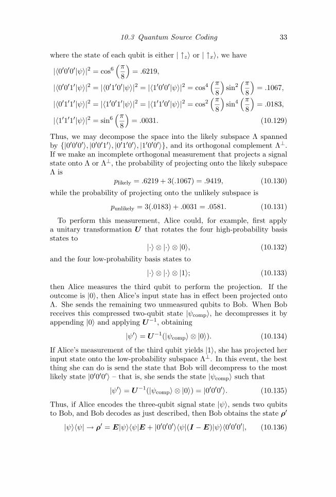
where the state of each qubit is either | ↑z〉 or | ↑x〉, we have
|〈0′0′0′|ψ〉|2 = cos6(π
8
)= .6219,
|〈0′0′1′|ψ〉|2 = |〈0′1′0′|ψ〉|2 = |〈1′0′0′|ψ〉|2 = cos4(π
8
)sin2
(π8
)= .1067,
|〈0′1′1′|ψ〉|2 = |〈1′0′1′|ψ〉|2 = |〈1′1′0′|ψ〉|2 = cos2(π
8
)sin4
(π8
)= .0183,
|〈1′1′1′|ψ〉|2 = sin6(π
8
)= .0031. (10.129)
Thus, we may decompose the space into the likely subspace Λ spannedby |0′0′0′〉, |0′0′1′〉, |0′1′0′〉, |1′0′0′〉, and its orthogonal complement Λ⊥.If we make an incomplete orthogonal measurement that projects a signalstate onto Λ or Λ⊥, the probability of projecting onto the likely subspaceΛ is
plikely = .6219 + 3(.1067) = .9419, (10.130)
while the probability of projecting onto the unlikely subspace is
punlikely = 3(.0183) + .0031 = .0581. (10.131)
To perform this measurement, Alice could, for example, first applya unitary transformation U that rotates the four high-probability basisstates to
|·〉 ⊗ |·〉 ⊗ |0〉, (10.132)
and the four low-probability basis states to
|·〉 ⊗ |·〉 ⊗ |1〉; (10.133)
then Alice measures the third qubit to perform the projection. If theoutcome is |0〉, then Alice’s input state has in effect been projected ontoΛ. She sends the remaining two unmeasured qubits to Bob. When Bobreceives this compressed two-qubit state |ψcomp〉, he decompresses it byappending |0〉 and applying U−1, obtaining
|ψ′〉 = U−1(|ψcomp〉 ⊗ |0〉). (10.134)
If Alice’s measurement of the third qubit yields |1〉, she has projected herinput state onto the low-probability subspace Λ⊥. In this event, the bestthing she can do is send the state that Bob will decompress to the mostlikely state |0′0′0′〉 – that is, she sends the state |ψcomp〉 such that
|ψ′〉 = U−1(|ψcomp〉 ⊗ |0〉) = |0′0′0′〉. (10.135)
Thus, if Alice encodes the three-qubit signal state |ψ〉, sends two qubitsto Bob, and Bob decodes as just described, then Bob obtains the state ρ′
|ψ〉〈ψ| → ρ′ = E|ψ〉〈ψ|E + |0′0′0′〉〈ψ|(I −E)|ψ〉〈0′0′0′|, (10.136)

34 10 Quantum Shannon Theory
where E is the projection onto Λ. The fidelity achieved by this procedureis
F = 〈ψ|ρ′|ψ〉 = (〈ψ|E|ψ〉)2 + (〈ψ|(I −E)|ψ〉)(〈ψ|0′0′0′〉)2
= (.9419)2 + (.0581)(.6219) = .9234. (10.137)
This is indeed better than the naive procedure of sending two of the threequbits each with perfect fidelity.
As we consider longer messages with more letters, the fidelity of thecompression improves, as long as we don’t try to compress too much.The Von-Neumann entropy of the one-qubit ensemble is
H(ρ) = H(cos2
π
8
)= .60088 . . . (10.138)
Therefore, according to Schumacher’s theorem, we can shorten a longmessage by the factor, say, .6009, and still achieve very good fidelity.
10.3.2 Schumacher compression in general
The key to Shannon’s noiseless coding theorem is that we can code thetypical sequences and ignore the rest, without much loss of fidelity. Toquantify the compressibility of quantum information, we promote thenotion of a typical sequence to that of a typical subspace. The key toSchumacher’s noiseless quantum coding theorem is that we can code thetypical subspace and ignore its orthogonal complement, without muchloss of fidelity.
We consider a message of n letters where each letter is a pure quantumstate drawn from the ensemble |ϕ(x)〉, p(x), so that the density operatorof a single letter is
ρ =∑x
p(x)|ϕ(x)〉〈ϕ(x)|. (10.139)
Since the letters are drawn independently, the density operator of theentire message is
ρ⊗n ≡ ρ⊗ · · · ⊗ ρ. (10.140)
We claim that, for n large, this density matrix has nearly all of its sup-port on a subspace of the full Hilbert space of the messages, where thedimension of this subspace asymptotically approaches 2nH(ρ).
This claim follows directly from the corresponding classical statement,for we may consider ρ to be realized by an ensemble of orthonormal purestates, its eigenstates, where the probability assigned to each eigenstateis the corresponding eigenvalue. In this basis our source of quantuminformation is effectively classical, producing messages which are tensor

10.3 Quantum Source Coding 35
products of ρ eigenstates, each with a probability given by the productof the corresponding eigenvalues. For a specified n and δ, define the δ-typical subspace Λ as the space spanned by the eigenvectors of ρ⊗n witheigenvalues λ satisfying
2−n(H−δ) ≥ λ ≥ 2−n(H+δ). (10.141)
Borrowing directly from Shannon’s argument, we infer that for any δ, ε >0 and n sufficiently large, the sum of the eigenvalues of ρ⊗n that obeythis condition satisfies
tr(ρ⊗nE) ≥ 1− ε, (10.142)
where E denotes the projection onto the typical subspace Λ, and thenumber dim(Λ) of such eigenvalues satisfies
2n(H+δ) ≥ dim(Λ) ≥ (1− ε)2n(H−δ). (10.143)
Our coding strategy is to send states in the typical subspace faithfully.We can make a measurement that projects the input message onto eitherΛ or Λ⊥; the outcome will be Λ with probability pΛ = tr(ρ⊗nE) ≥ 1− ε.In that event, the projected state is coded and sent. Asymptotically, theprobability of the other outcome becomes negligible, so it matters littlewhat we do in that case.
The coding of the projected state merely packages it so it can be carriedby a minimal number of qubits. For example, we apply a unitary changeof basis U that takes each state |ψtyp〉 in Λ to a state of the form
U |ψtyp〉 = |ψcomp〉 ⊗ |0rest〉, (10.144)
where |ψcomp〉 is a state of n(H + δ) qubits, and |0rest〉 denotes the state|0〉 ⊗ . . . ⊗ |0〉 of the remaining qubits. Alice sends |ψcomp〉 to Bob, whodecodes by appending |0rest〉 and applying U−1.
Suppose that|ϕ(~x)〉 = |ϕ(x1)〉 ⊗ . . .⊗ |ϕ(xn)〉, (10.145)
denotes any one of the n-letter pure state messages that might be sent.After coding, transmission, and decoding are carried out as just described,Bob has reconstructed a state
|ϕ(~x)〉〈ϕ(~x)| 7→ ρ′(~x) = E|ϕ(~x)〉〈ϕ(~x)|E+ ρJunk(~x)〈ϕ(~x)|(I −E)|ϕ(~x)〉, (10.146)
where ρJunk(~x) is the state we choose to send if the measurement yieldsthe outcome Λ⊥. What can we say about the fidelity of this procedure?

36 10 Quantum Shannon Theory
The fidelity varies from message to message, so we consider the fidelityaveraged over the ensemble of possible messages:
F =∑~x
p(~x)〈ϕ(~x)|ρ′(~x)|ϕ(~x)〉
=∑~x
p(~x)〈ϕ(~x)|E|ϕ(~x)〉〈ϕ(~x)|E|ϕ(~x)〉
+∑~x
p(~x)〈ϕ(~x)|ρJunk(~x)|ϕ(~x)〉〈ϕ(~x)|I −E|ϕ(~x)〉
≥∑~x
p(~x)〈ϕ(~x)|E|ϕ(~x)〉2, (10.147)
where the last inequality holds because the “Junk” term is nonnegative.Since any real number z satisfies
(z − 1)2 ≥ 0, or z2 ≥ 2z − 1, (10.148)
we have (setting z = 〈ϕ(~x)|E|ϕ(~x)〉)
〈ϕ(~x)|E|ϕ(~x)〉2 ≥ 2〈ϕ(~x)|E|ϕ(~x)〉 − 1, (10.149)
and hence
F ≥∑~x
p(~x)(2〈ϕ(~x)|E|ϕ(~x)〉 − 1)
= 2 tr(ρ⊗nE)− 1 ≥ 2(1− ε)− 1 = 1− 2ε. (10.150)
Since ε and δ can be as small as we please, we have shown that it ispossible to compress the message to n(H + o(1)) qubits, while achievingan average fidelity that becomes arbitrarily good as n gets large.
Is further compression possible? Let us suppose that Bob will decodethe message ρcomp(~x) that he receives by appending qubits and applyinga unitary transformation U−1, obtaining
ρ′(~x) = U−1(ρcomp(~x)⊗ |0〉〈0|)U (10.151)
(“unitary decoding”), and suppose that ρcomp(~x) has been compressedto n(H − δ′) qubits. Then, no matter how the input messages have beenencoded, the decoded messages are all contained in a subspace Λ′ of Bob’sHilbert space with dim(Λ′) = 2n(H−δ′).
If the input message is |ϕ(~x)〉, then the density operator reconstructedby Bob can be diagonalized as
ρ′(~x) =∑a~x
|a~x〉λa~x〈a~x|, (10.152)

10.3 Quantum Source Coding 37
where the |a~x〉’s are mutually orthogonal states in Λ′. The fidelity of thereconstructed message is
F (~x) = 〈ϕ(~x)|ρ′(~x)|ϕ(~x)〉
=∑a~x
λa~x〈ϕ(~x)|a~x〉〈a~x|ϕ(~x)〉
≤∑a~x
〈ϕ(~x)|a~x〉〈a~x|ϕ(~x)〉 ≤ 〈ϕ(~x)|E′|ϕ(~x)〉, (10.153)
where E′ denotes the orthogonal projection onto the subspace Λ′. Theaverage fidelity therefore obeys
F =∑~x
p(~x)F (~x) ≤∑~x
p(~x)〈ϕ(~x)|E′|ϕ(~x)〉 = tr(ρ⊗nE′). (10.154)
But, according to the Ky Fan dominance principle discussed in §10.2.2,since E′ projects onto a space of dimension 2n(H−δ′), tr(ρ⊗nE′) can beno larger than the sum of the 2n(H−δ′) largest eigenvalues of ρ⊗n. Theδ-typical eigenvalues of ρ⊗n are no smaller than 2−n(H−δ), so the sum ofthe 2n(H−δ′) largest eigenvalues can be bounded above:
tr(ρ⊗nE′) ≤ 2n(H−δ′)2−n(H−δ) + ε = 2−n(δ′−δ) + ε, (10.155)
where the + ε accounts for the contribution from the atypical eigenvalues.Since we may choose ε and δ as small as we please for sufficiently largen, we conclude that the average fidelity F gets small as n → ∞ if wecompress to H(ρ) − Ω(1) qubits per letter. We find, then, that H(ρ)qubits per letter is the optimal compression of the quantum informationthat can be achieved if we are to obtain good fidelity as n goes to infinity.This is Schumacher’s quantum source coding theorem.
The above argument applies to any conceivable encoding scheme, butonly to a restricted class of decoding schemes, unitary decodings. Theextension of the argument to general decoding schemes is sketched in§10.6.3. The conclusion is the same. The point is that n(H − δ) qubitsare too few to faithfully encode the typical subspace.
There is another useful way to think about Schumacher’s quantum com-pression protocol. Suppose that Alice’s density operator ρ⊗nA has a pu-rification |ψ〉RA which Alice shares with Robert. Alice wants to conveyher share of |ψ〉RA to Bob with high fidelity, sending as few qubits to Bobas possible. To accomplish this task, Alice can use the same procedureas described above, attempting to compress the state of A by projectingonto its typical subspace Λ. Alice’s projection succeeds with probability
P (E) = 〈ψ|I ⊗E|ψ〉 = tr(ρ⊗nE
)≥ 1− ε, (10.156)
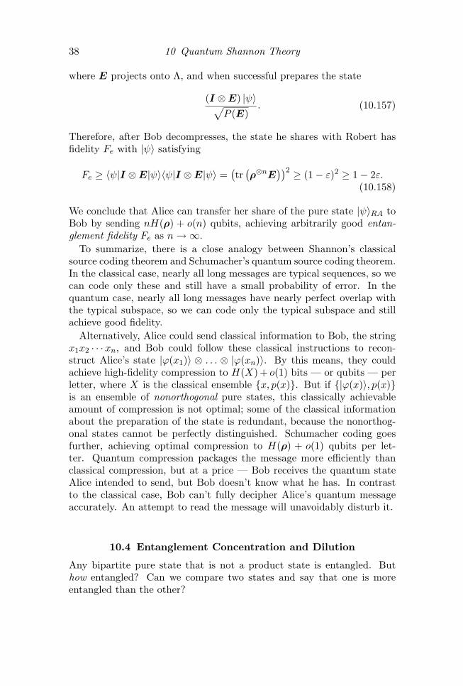
38 10 Quantum Shannon Theory
where E projects onto Λ, and when successful prepares the state
(I ⊗E) |ψ〉√P (E)
. (10.157)
Therefore, after Bob decompresses, the state he shares with Robert hasfidelity Fe with |ψ〉 satisfying
Fe ≥ 〈ψ|I ⊗E|ψ〉〈ψ|I ⊗E|ψ〉 =(tr(ρ⊗nE
))2 ≥ (1− ε)2 ≥ 1− 2ε.(10.158)
We conclude that Alice can transfer her share of the pure state |ψ〉RA toBob by sending nH(ρ) + o(n) qubits, achieving arbitrarily good entan-glement fidelity Fe as n→∞.
To summarize, there is a close analogy between Shannon’s classicalsource coding theorem and Schumacher’s quantum source coding theorem.In the classical case, nearly all long messages are typical sequences, so wecan code only these and still have a small probability of error. In thequantum case, nearly all long messages have nearly perfect overlap withthe typical subspace, so we can code only the typical subspace and stillachieve good fidelity.
Alternatively, Alice could send classical information to Bob, the stringx1x2 · · ·xn, and Bob could follow these classical instructions to recon-struct Alice’s state |ϕ(x1)〉 ⊗ . . . ⊗ |ϕ(xn)〉. By this means, they couldachieve high-fidelity compression to H(X) + o(1) bits — or qubits — perletter, where X is the classical ensemble x, p(x). But if |ϕ(x)〉, p(x)is an ensemble of nonorthogonal pure states, this classically achievableamount of compression is not optimal; some of the classical informationabout the preparation of the state is redundant, because the nonorthog-onal states cannot be perfectly distinguished. Schumacher coding goesfurther, achieving optimal compression to H(ρ) + o(1) qubits per let-ter. Quantum compression packages the message more efficiently thanclassical compression, but at a price — Bob receives the quantum stateAlice intended to send, but Bob doesn’t know what he has. In contrastto the classical case, Bob can’t fully decipher Alice’s quantum messageaccurately. An attempt to read the message will unavoidably disturb it.
10.4 Entanglement Concentration and Dilution
Any bipartite pure state that is not a product state is entangled. Buthow entangled? Can we compare two states and say that one is moreentangled than the other?

10.4 Entanglement Concentration and Dilution 39
For example, consider the two bipartite states
|φ+〉 =1√2(|00〉+ |11〉),
|ψ〉 =1√2|00〉+
12|11〉+
12|22〉. (10.159)
|φ+〉 is a maximally entangled state of two qubits, while |ψ〉 is a partiallyentangled state of two qutrits. Which is more entangled?
It is not immediately clear that the question has a meaningful answer.Why should it be possible to find an unambiguous way of ordering allbipartite pure states according to their degree of entanglement? Can wecompare a pair of qutrits with a pair of qubits any more than we cancompare apples and oranges?
A crucial feature of entanglement is that it cannot be created by localoperations and classical communication (LOCC). In particular, if Aliceand Bob share a bipartite pure state, its Schmidt number does not increaseif Alice or Bob performs a unitary transformation on her/his share ofthe state, nor if Alice or Bob measures her/his share, even if Alice andBob exchange classical messages about their actions and measurementoutcomes. Therefore, any quantitative measure of entanglement shouldhave the property that LOCC cannot increase it, and it should also vanishfor an unentangled product state. An obvious candidate is the Schmidtnumber, but on reflection it does not seem very satisfactory. Consider
|ψε〉 =√
1− 2|ε|2 |00〉+ ε|11〉+ ε|22〉, (10.160)
which has Schmidt number 3 for any |ε| > 0. Do we really want to saythat |ψε〉 is “more entangled” than |φ+〉? Entanglement, after all, can beregarded as a resource — we might plan to use it for teleportation, forexample — and it seems clear that |ψε〉 (for |ε| 1) is a less valuableresource than |φ+〉.
It turns out, though, that there is a natural and useful way to quantifythe entanglement of any bipartite pure state. To compare two states,we use LOCC to convert both states to a common currency that can becompared directly. The common currency is maximal entanglement, andthe amount of shared entanglement can be expressed in units of Bell pairs(maximally entangled two-qubit states), also called ebits of entanglement.
To quantify the entanglement of a particular bipartite pure state,|ψ〉AB, imagine preparing n identical copies of that state. Alice and Bobshare a large supply of maximally entangled Bell pairs. Using LOCC,they are to convert k Bell pairs (|φ+〉AB)⊗k) to n high-fidelity copies ofthe desired state (|ψ〉AB)⊗n). What is the minimum number kmin of Bellpairs with which they can perform this task?

40 10 Quantum Shannon Theory
To obtain a precise answer, we consider the asymptotic setting, requir-ing arbitrarily high-fidelity conversion in the limit of large n. We say thata rate R of conversion from |φ+〉 to |ψ〉 is asymptotically achievable if forany ε, δ > 0, there is an LOCC protocol with
k
n≤ R+ δ, (10.161)
which prepares the target state |ψ+〉⊗n with fidelity F ≥ 1−ε. We definethe entanglement cost EC of |ψ〉 as the infimum of achievable conversionrates:
EC(|ψ〉) := inf achievable rate for creating |ψ〉 from Bell pairs .(10.162)
Asymptotically, we can create many copies of |ψ〉 by consuming EC Bellpairs per copy.
Now imagine that n copies of |ψ〉AB are already shared by Alice andBob. Using LOCC, Alice and Bob are to convert (|ψ〉AB)⊗n back to thestandard currency: k′ Bell pairs |φ+〉⊗k′AB . What is the maximum numberk′max of Bell pairs they can extract from |ψ〉⊗nAB? In this case we say thata rate R′ of conversion from |ψ〉 to |φ+〉 is asymptotically achievable if forany ε, δ > 0, there is an LOCC protocol with
k′
n≥ R′ − δ, (10.163)
which prepares the target state |φ+〉⊗k′ with fidelity F ≥ 1−ε. We definethe distillable entanglement ED of |ψ〉 as the supremum of achievableconversion rates:
ED(|ψ〉) := sup achievable rate for distilling Bell pairs from |ψ〉 .(10.164)
Asymptotically, we can convert many copies of |ψ〉 to Bell pairs, obtainingED Bell pairs per copy of |ψ〉 consumed.
Since it is an in inviolable principle that LOCC cannot create entan-glement, it is certain that
ED(|ψ〉) ≤ EC(|ψ〉); (10.165)
otherwise Alice and Bob could increase their number of shared Bell pairsby converting them to copies of |ψ〉 and then back to Bell pairs. In factthe entanglement cost and distillable entanglement are equal for bipartitepure states. (The story is more complicated for bipartite mixed states;see §10.5.) Therefore, for pure states at least we may drop the subscript,using E(|ψ〉) to denote the entanglement of |ψ〉. We don’t need to dis-tinguish between entanglement cost and distillable entanglement because

10.4 Entanglement Concentration and Dilution 41
conversion of entanglement from one form to another is an asymptoticallyreversible process. E quantifies both what we have to pay in Bell pairs tocreate |ψ〉, and value of |ψ〉 in Bell pairs for performing tasks like quantumteleportation which consume entanglement.
But what is the value of E(|ψ〉AB)? Perhaps you can guess — it is
E(|ψ〉AB) = H(ρA) = H(ρB), (10.166)
the Von Neumann entropy of Alice’s density operator ρA (or equivalentlyBob’s density operator ρB). This is clearly the right answer in the casewhere |ψ〉AB is a product of k Bell pairs. In that case ρA (or ρB) is 1
2Ifor each qubit in Alice’s possession
ρA =(
12I
)⊗k, (10.167)
and
H(ρA) = k H
(12I
)= k. (10.168)
How do we see that E = H(ρA) is the right answer for any bipartite purestate?
Though it is perfectly fine to use Bell pairs as the common currencyfor comparing bipartite entangled states, in the asymptotic setting it issimpler and more natural to allow fractions of a Bell pair, which is whatwe’ll do here. That is, we’ll consider a maximally entangled state of two d-dimensional systems to be log2 d Bell pairs, even if d is not a power of two.So our goal will be to show that Alice and Bob can use LOCC to convertshared maximal entanglement of systems with dimension d = 2n(H(ρA)+δ)
into n copies of |ψ〉, for any positive δ and with arbitrarily good fidelityas n→∞, and conversely that Alice and Bob can use LOCC to convertn copies of |ψ〉 into a shared maximally entangled state of d-dimensionalsystems with arbitrarily good fidelity, where d = 2n(H(ρA)−δ). This sufficesto demonstrate that EC(|ψ〉) = ED(|ψ〉) = H(ρA).
First let’s see that if Alice and Bob share k = n(H(ρA) + δ) Bellpairs, then they can prepare |ψ〉⊗nAB with high fidelity using LOCC. Theyperform this task, called entanglement dilution, by combining quantumteleportation with Schumacher compression. To get started, Alice locallycreates n copies of |ψ〉AC , where A and C are systems she controls in herlaboratory. Next she wishes to teleport the Cn share of these copies toBob, but to minimize the consumption of Bell pairs, she should compressCn before teleporting it.
If A and C are d-dimensional, then the bipartite state |ψ〉AC can beexpressed in terms of its Schmidt basis as
|ψ〉AC =√p0 |00〉+
√p1 |11〉+ . . .+
√pd−1 |d−1, d−1〉, (10.169)

42 10 Quantum Shannon Theory
and n copies of the state can be expressed as
|ψ〉⊗nAC =d−1∑
x1,...,xn=0
√p(x1) . . . p(xn) |x1x2 . . . xn〉An ⊗ |x1x2 . . . xn〉Cn
=∑~x
√p(~x) |~x〉An ⊗ |~x〉Cn , (10.170)
where∑
~x p(~x) = 1. If Alice attempts to project onto the δ-typical sub-space of Cn, she succeeds with high probability
P =∑
δ−typical ~x
p(~x) ≥ 1− ε (10.171)
and when successful prepares the post-measurement state
|Ψ〉AnCn = P−1/2∑
δ−typical ~x
√p(~x) |~x〉An ⊗ |~x〉Cn , (10.172)
such that
〈Ψ|ψ⊗n〉 = P−1/2∑
δ−typical ~x
p(~x) =√P ≥
√1− ε. (10.173)
Since the typical subspace has dimension at most 2n(H(ρ)+δ), Alice canteleport the Cn half of |Ψ〉 to Bob with perfect fidelity using no more thann(H(ρ) + δ) Bell pairs shared by Alice and Bob. The teleportation usesLOCC: Alice’s entangled measurement, classical communication from Al-ice to Bob to convey the measurement outcome, and Bob’s unitary trans-formation conditioned on the outcome. Finally, after the teleportation,Bob decompresses, so that Alice and Bob share a state which has highfidelity with |ψ〉⊗nAB. This protocol demonstrates that the entanglementcost EC of |ψ〉 is not more than H(ρA).
Now consider the distillable entanglement ED. Suppose Alice and Bobshare the state |ψ〉⊗nAB. Since |ψ〉AB is, in general, a partially entangledstate, the entanglement that Alice and Bob share is in a diluted form.They wish to concentrate their shared entanglement, squeezing it downto the smallest possible Hilbert space; that is, they want to convert it tomaximally-entangled pairs. We will show that Alice and Bob can “distill”at least
k′ = n(H(ρA)− δ) (10.174)
Bell pairs from |ψ〉⊗nAB, with high likelihood of success.To illustrate the concentration of entanglement, imagine that Alice and
Bob have n copies of the two-qubit state |ψ〉, which is
|ψ(p)〉 =√
1− p |00〉+√p |11〉, (10.175)

10.4 Entanglement Concentration and Dilution 43
where 0 ≤ p ≤ 1, when expressed in its Schmidt basis. That is, Alice andBob share the state
|ψ(p)〉⊗n = (√
1− p |00〉+√p |11〉)⊗n. (10.176)
When we expand this state in the |0〉, |1〉 basis, we find 2n terms, ineach of which Alice and Bob hold exactly the same binary string of lengthn.
Now suppose Alice (or Bob) performs a local measurement on her (his)n qubits, measuring the total spin along the z-axis
σ(total)3 =
n∑i=1
σ(i)3 . (10.177)
Equivalently, the measurement determines the Hamming weight of Alice’sn qubits, the number of |1〉’s in Alice’s n-bit string; that is, the numberof spins pointing up.
In the expansion of |ψ(p)〉⊗n there are(nm
)terms in which Alice’s
string has Hamming weight m, each occurring with the same amplitude:(1− p)(n−m)/2 pm/2. Hence the probability that Alice’s measurement findsHamming weight m is
p(m) =(n
m
)(1− p)n−mpm. (10.178)
Furthermore, because Alice is careful not to acquire any additional infor-mation besides the Hamming weight when she conducts the measurement,by measuring the Hamming weight m she prepares a uniform superpo-sition of all
(nm
)strings with m up spins. Because Alice and Bob have
perfectly correlated strings, if Bob were to measure the Hamming weightof his qubits he would find the same outcome as Alice. Alternatively,Alice could report her outcome to Bob in a classical message, saving Bobthe trouble of doing the measurement himself. Thus, Alice and Bob sharea maximally entangled state
D∑i=1
|i〉A ⊗ |i〉B, (10.179)
where the sum runs over the D =(nm
)strings with Hamming weight m.
For n large the binomial distribution p(m) approaches a sharplypeaked function of m with mean µ = np and variance σ2 = np(1 − p).Hence the probability of a large deviation from the mean,
|m− np| = Ω(n), (10.180)

44 10 Quantum Shannon Theory
is p = exp (−Ω(n)). Using Stirling’s approximation, it then follows that
2n(H(p)−o(1)) ≤ D ≤ 2n(H(p)+o(1)). (10.181)
with probability approaching one as n → ∞, where H(p) = −p log2 p −(1 − p) log2(1 − p) is the entropy function. Thus with high probabilityAlice and Bob share a maximally entangled state of Hilbert spaces HA
and HB with dim(HA) = dim(HB) = D and log2D ≥ n(H(p) − δ). Inthis sense Alice and Bob can distill H(p)− δ Bell pairs per copy of |ψ〉AB.
Though the number m of up spins that Alice (or Bob) finds in her (his)measurement is typically close to np, it can fluctuate about this value.Sometimes Alice and Bob will be lucky, and then will manage to distillmore than H(p) Bell pairs per copy of |ψ(p)〉AB. But the probability ofdoing substantially better becomes negligible as n→∞.
The same idea applies to bipartite pure states in larger Hilbert spaces.If A and B are d-dimensional systems, then |ψ〉AB has the Schmidt de-composition
|ψ(X)〉AB =d−1∑i=0
√p(x) |x〉A ⊗ |x〉B, (10.182)
where X is the classical ensemble x, p(x), and H(ρA) = H(ρB) =H(X). The Schmidt decomposition of n copies of ψ〉 is
d−1∑x1,x2,...,xn=0
√p(x1)p(x2) . . . p(xn) |x1x2 . . . xn〉An ⊗ |x1x2 . . . xn〉Bn .
(10.183)Now Alice (or Bob) can measure the total number of |0〉’s, the totalnumber of |1〉’s, etc. in her (his) possession. If she finds m0|0〉’s, m1|1〉’s,etc., then her measurement prepares a maximally entangled state withSchmidt number
D(m0,m1, . . . ,md−1) =n!
m0!m1! . . .md−1!(10.184)
and this outcome occurs with probability
p(m) = D(m0,m1, . . . ,md−1)p(0)m0p(1)m1 . . . p(d−1)md−1 . (10.185)
For n large, Alice will typically findmx ≈ np(x), and again the probabilityof a large deviation is small, so that, from Stirling’s approximation
2n(H(X)−o(1)) ≤ D ≤ 2n(H(X)+o(1)) (10.186)
with high probability. Thus, asymptotically for n→∞, n(H(ρA)− o(1))high-fidelity Bell pairs can be distilled from n copies of |ψ〉, establishingthat ED(|ψ〉) ≥ H(ρA), and therefore ED(|ψ〉) = EC(|ψ〉) = E(|ψ〉).

10.5 Quantifying Mixed-State Entanglement 45
This entanglement concentration protocol uses local operations butdoes not require any classical communication. When Alice and Bob do thesame measurement they always get the same outcome, so there is no needfor them to communicate. Classical communication really is necessary,though, to perform entanglement dilution. The protocol we describedhere, based on teleportation, requires two bits of classical one-way com-munication per Bell pair consumed; in a more clever protocol this can bereduced to O(
√n) bits, but no further. Since the classical communica-
tion cost is sublinear in n, the number of bits of classical communicationneeded per copy of |ψ〉 becomes negligible in the limit n→∞.
10.5 Quantifying Mixed-State Entanglement
10.5.1 Asymptotic irreversibility under LOCC
The entanglement cost EC and the distillable entanglement ED are nat-ural and operationally meaningful ways to quantify entanglement. It’squite satisfying to find that, because entanglement dilution and concen-tration are asymptotically reversible for pure states, these two measures ofpure-state bipartite entanglement agree, and provide another operationalrole for the Von Neumann entropy of a marginal quantum state.
We can define EC and ED for bipartite mixed states just as we didfor pure states, but the story is more complicated — when we preparemany copies of a mixed state shared by Alice and Bob, the dilution of Bellpairs is not in general reversible, even asymptotically, and the distillableentanglement can be strictly less than the entanglement cost, though itcan never be larger. There are even bipartite mixed states with nonzeroentanglement cost and zero distillable entanglement, a phenomenon calledbound entanglement. This irreversibility is not shocking; any bipartiteoperation which maps many copies of the pure state |φ+〉AB to manycopies of the mixed state ρAB necessarily discards some information tothe environment, and we don’t normally expect a process that forgetsinformation to be reversible.
This separation between EC and ED raises the question, what is thepreferred way to quantify the amount of entanglement when two partiesshare a mixed quantum state? The answer is, it depends. Many differentmeasures of bipartite mixed-state entanglement have been proposed, eachwith its own distinctive advantages and disadvantages. Even though theydo not always agree, both EC and ED are certainly valid measures. Afurther distinction can be made between the rate ED1 at which entangle-ment can be distilled with one-way communication between the parties,and the rate ED with two-way communication. There are bipartite mixedstates for which ED > ED1, and even states for which ED is nonzero while

46 10 Quantum Shannon Theory
ED1 is zero. In contrast to the pure-state case, we don’t have nice formu-las for the values of the various entanglement measures, though there areuseful upper and lower bounds. We will derive a lower bound on ED1 in§10.8.2 (the hashing inequality).
There are certain properties that any reasonable measure of bipartitequantum entanglement should have. The most important is that it mustnot increase under local operations and classical communication, becausequantum entanglement cannot be created by LOCC alone. A functionon bipartite states that is nonincreasing under LOCC is called an en-tanglement monotone. Note that an entanglement monotone will also beinvariant under local unitary operations UAB = UA ⊗ UB, for if UAB canreduce the entanglement for any state, its inverse can increase entangle-ment.
A second important property is that a bipartite entanglement measuremust vanish for separable states. Recall from Chapter 4 that a bipartitemixed state is separable if it can be expressed as a convex combinationof product states,
ρAB =∑x
p(x) |α(x)〉〈α(x)|A ⊗ |β(x)〉〈β(x)|B. (10.187)
A separable state is not entangled, as it can be created using LOCC.Via classical communication, Alice and Bob can establish a shared sourceof randomness, the distribution X = x, p(x). Then they may jointlysample from X; if the outcome is x, Alice prepares |α(x)〉 while Bobprepares |β(x)〉.
A third desirable property for a bipartite entanglement measure is thatit should agree with E = EC = ED for bipartite pure states. Both theentanglement cost and the distillable entanglement respect all three ofthese properties.
We remark in passing that, despite the irreversibility of entanglementdilution under LOCC, there is a mathematically viable way to formulatea reversible theory of bipartite entanglement which applies even to mixedstates. In this formulation, we allow Alice and Bob to perform arbitrarybipartite operations that are incapable of creating entanglement; theseinclude LOCC as well as additional operations which cannot be realizedusing LOCC. In this framework, dilution and concentration of entan-glement become asymptotically reversible even for mixed states, and aunique measure of entanglement can be formulated characterizing the op-timal rate of conversion between copies of ρAB and Bell pairs using thesenon-entangling operations.
Irreversible bipartite entanglement theory under LOCC, and also thereversible theory under non-entangling bipartite operations, are both ex-amples of resource theories. In the resource theory framework, one or

10.5 Quantifying Mixed-State Entanglement 47
more parties are able to perform some restricted class of operations, andthey are capable of preparing a certain restricted class of states usingthese operations. In addition, the parties may also have access to re-source states, which are outside the class they can prepare on their own.Using their restricted operations, they can transform resource states fromone form to another, or consume resource states to perform operationsbeyond what they could achieve with their restricted operations alone.The name “resource state” conveys that such states are valuable becausethey may be consumed to do useful things.
In a two-party setting, where LOCC is allowed or more general non-entangling operations are allowed, bipartite entangled states may be re-garded as a valuable resource. Resource theory also applies if the allowedoperations are required to obey certain symmetries; then states breakingthis symmetry become a resource. In thermodynamics, states deviat-ing from thermal equilibrium are a resource. Entanglement theory, as aparticularly well developed resource theory, provides guidance and toolswhich are broadly applicable to many different interesting situations.
10.5.2 Squashed entanglement
As an example of an alternative bipartite entanglement measure, considerthe squashed entanglement Esq, defined by
Esq(ρAB) = inf
12I(A;B|C) : ρAB = trC (ρABC)
(10.188)
The squashed entanglement of ρAB is the greatest lower bound on thequantum conditional mutual information of all possible extensions of ρABto a tripartite state ρABC ; it can be shown to be an entanglement mono-tone. The locution “squashed” conveys that choosing an optimal condi-tioning system C squashes out the non-quantum correlations between Aand B.
For pure states the extension is superfluous, so that
Esq(|ψ〉AB) =12I(A;B) = H(A) = H(B) = E(|ψ〉AB). (10.189)
For a separable state, we may choose the extension
ρABC =∑x
p(x) |α(x)〉〈α(x)|A ⊗ |β(x)〉〈β(x)|B ⊗ |x〉〈x|C . (10.190)
where |x〉C is an orthonormal set; the state ρABC has the block-diagonalform eq.(10.82) and hence I(A;B|C) = 0. Conversely, if ρAB has anyextension ρABC with I(A;B|C) = 0, then ρABC has the form eq.(10.82)and therefore ρAB is separable.
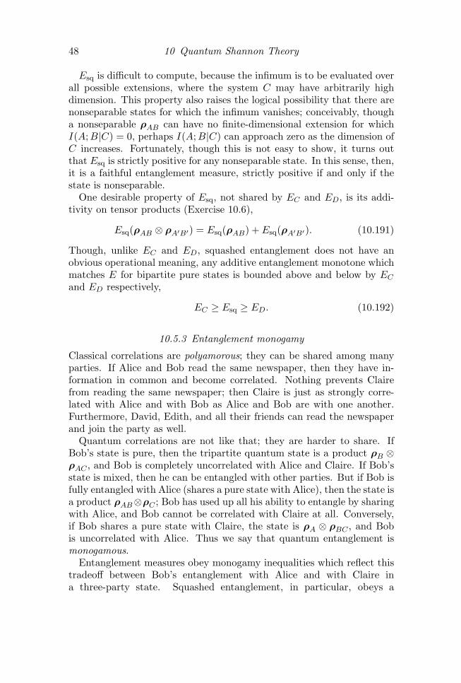
48 10 Quantum Shannon Theory
Esq is difficult to compute, because the infimum is to be evaluated overall possible extensions, where the system C may have arbitrarily highdimension. This property also raises the logical possibility that there arenonseparable states for which the infimum vanishes; conceivably, thougha nonseparable ρAB can have no finite-dimensional extension for whichI(A;B|C) = 0, perhaps I(A;B|C) can approach zero as the dimension ofC increases. Fortunately, though this is not easy to show, it turns outthat Esq is strictly positive for any nonseparable state. In this sense, then,it is a faithful entanglement measure, strictly positive if and only if thestate is nonseparable.
One desirable property of Esq, not shared by EC and ED, is its addi-tivity on tensor products (Exercise 10.6),
Esq(ρAB ⊗ ρA′B′) = Esq(ρAB) + Esq(ρA′B′). (10.191)
Though, unlike EC and ED, squashed entanglement does not have anobvious operational meaning, any additive entanglement monotone whichmatches E for bipartite pure states is bounded above and below by ECand ED respectively,
EC ≥ Esq ≥ ED. (10.192)
10.5.3 Entanglement monogamy
Classical correlations are polyamorous; they can be shared among manyparties. If Alice and Bob read the same newspaper, then they have in-formation in common and become correlated. Nothing prevents Clairefrom reading the same newspaper; then Claire is just as strongly corre-lated with Alice and with Bob as Alice and Bob are with one another.Furthermore, David, Edith, and all their friends can read the newspaperand join the party as well.
Quantum correlations are not like that; they are harder to share. IfBob’s state is pure, then the tripartite quantum state is a product ρB ⊗ρAC , and Bob is completely uncorrelated with Alice and Claire. If Bob’sstate is mixed, then he can be entangled with other parties. But if Bob isfully entangled with Alice (shares a pure state with Alice), then the state isa product ρAB⊗ρC ; Bob has used up all his ability to entangle by sharingwith Alice, and Bob cannot be correlated with Claire at all. Conversely,if Bob shares a pure state with Claire, the state is ρA ⊗ ρBC , and Bobis uncorrelated with Alice. Thus we say that quantum entanglement ismonogamous.
Entanglement measures obey monogamy inequalities which reflect thistradeoff between Bob’s entanglement with Alice and with Claire ina three-party state. Squashed entanglement, in particular, obeys a

10.5 Quantifying Mixed-State Entanglement 49
monogamy relation following easily from its definition, which was ourprimary motivation for introducing this quantity; we have
Esq(A;B) + Esq(A;C) ≤ Esq(A;BC). (10.193)
In particular, in the case of a pure tripartite state, Esq = H(A) is the(pure-state) entanglement shared between A and BC. The inequality issaturated if Alice’s system is divided into subsystems A1 and A2 suchthat the tripartite pure state is
|ψ〉ABC = |ψ1〉A1B ⊗ |ψ2〉A2C . (10.194)
In general, combining eq.(10.192) with eq.(10.193) yields
ED(A;B) + ED(A;C) ≤ EC(A;BC); (10.195)
loosely speaking, the entanglement cost EC(A;BC) imposes a ceiling onAlice’s ability to entangle with Bob and Claire individually, requiringher to trade in some distillable entanglement with Bob to increase herdistillable entanglement with Claire.
To prove the monogamy relation eq.(10.193), we note that mutual in-formation obeys a chain rule which is really just a restatement of thedefinition of conditional mutual information:
I(A;BC) = I(A;C) + I(A;B|C). (10.196)
A similar equation follows directly from the definition if we condition ona fourth system D,
I(A;BC|D) = I(A;C|D) + I(A;B|CD). (10.197)
Now, Esq(A;BC) is the infimum of I(A;BC|D) over all possible exten-sions of ρABC to ρABCD. But since ρABCD is also an extension of ρABand ρAC , we have
I(A;BC|D) ≥ Esq(A;C) + Esq(A;B) (10.198)
for any such extension. Taking the infimum over all ρABCD yieldseq.(10.193).
A further aspect of monogamy arises when we consider extending aquantum state to more parties. We say that the bipartite state ρAB of sys-tems A and B is k-extendable if there is a (k+1)-part state ρAB1...Bk
whosemarginal state on ABj matches ρAB for each j = 1, 2, . . . k, and such thatρAB1...Bk
is invariant under permutations of the k systems B1, B2 . . . Bk.Separable states are k-extendable for every k, and entangled pure statesare not even 2-extendable. Every entangled mixed state fails to be k-extendable for some finite k, and we may regard the maximal value kmax
for which such a symmetric extension exists as a rough measure of howentangled the state is — bipartite entangled states with larger and largerkmax are closer and closer to being separable.
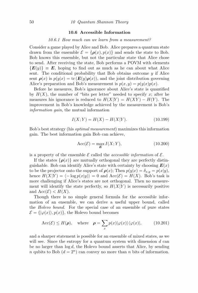
50 10 Quantum Shannon Theory
10.6 Accessible Information
10.6.1 How much can we learn from a measurement?
Consider a game played by Alice and Bob. Alice prepares a quantum statedrawn from the ensemble E = ρ(x), p(x) and sends the state to Bob.Bob knows this ensemble, but not the particular state that Alice choseto send. After receiving the state, Bob performs a POVM with elementsE(y) ≡ E, hoping to find out as much as he can about what Alicesent. The conditional probability that Bob obtains outcome y if Alicesent ρ(x) is p(y|x) = tr (E(y)ρ(x)), and the joint distribution governingAlice’s preparation and Bob’s measurement is p(x, y) = p(y|x)p(x).
Before he measures, Bob’s ignorance about Alice’s state is quantifiedby H(X), the number of “bits per letter” needed to specify x; after hemeasures his ignorance is reduced to H(X|Y ) = H(XY ) − H(Y ). Theimprovement in Bob’s knowledge achieved by the measurement is Bob’sinformation gain, the mutual information
I(X;Y ) = H(X)−H(X|Y ). (10.199)
Bob’s best strategy (his optimal measurement) maximizes this informationgain. The best information gain Bob can achieve,
Acc(E) = maxE
I(X;Y ), (10.200)
is a property of the ensemble E called the accessible information of E .If the states ρ(x) are mutually orthogonal they are perfectly distin-
guishable. Bob can identify Alice’s state with certainty by choosing E(x)to be the projector onto the support of ρ(x); Then p(y|x) = δx,y = p(x|y),hence H(X|Y ) = 〈− log p(x|y)〉 = 0 and Acc(E) = H(X). Bob’s task ismore challenging if Alice’s states are not orthogonal. Then no measure-ment will identify the state perfectly, so H(X|Y ) is necessarily positiveand Acc(E) < H(X).
Though there is no simple general formula for the accessible infor-mation of an ensemble, we can derive a useful upper bound, calledthe Holevo bound. For the special case of an ensemble of pure statesE = |ϕ(x)〉, p(x), the Holevo bound becomes
Acc(E) ≤ H(ρ), where ρ =∑x
p(x)|ϕ(x)〉〈ϕ(x)|, (10.201)
and a sharper statement is possible for an ensemble of mixed states, as wewill see. Since the entropy for a quantum system with dimension d canbe no larger than log d, the Holevo bound asserts that Alice, by sendingn qubits to Bob (d = 2n) can convey no more than n bits of information.

10.6 Accessible Information 51
This is true even if Bob performs a sophisticated collective measurementon all the qubits at once, rather than measuring them one at a time.
Therefore, if Alice wants to convey classical information to Bob bysending qubits, she can do no better than treating the qubits as thoughthey were classical, sending each qubit in one of the two orthogonal states|0〉, |1〉 to transmit one bit. This statement is not so obvious. Alicemight try to stuff more classical information into a single qubit by sendinga state chosen from a large alphabet of pure single-qubit signal states,distributed uniformly on the Bloch sphere. But the enlarged alphabet isto no avail, because as the number of possible signals increases the signalsalso become less distinguishable, and Bob is not able to extract the extrainformation Alice hoped to deposit in the qubit.
If we can send information more efficiently by using an alphabet ofmutually orthogonal states, why should we be interested in the accessibleinformation for an ensemble of non-orthogonal states? There are manypossible reasons. Perhaps Alice finds it easier to send signals, like co-herent states, which are imperfectly distinguishable rather than mutuallyorthogonal. Or perhaps Alice sends signals to Bob through a noisy chan-nel, so that signals which are orthogonal when they enter the channel areimperfectly distinguishable by the time they reach Bob.
The accessible information game also arises when an experimentalphysicist tries to measure an unknown classical force using a quantumsystem as a probe. For example, to measure the z-component of a mag-netic field, we may prepare a spin-1
2 particle pointing in the x-direction;the spin precesses for time t in the unknown field, producing an ensem-ble of possible final states (which will be an ensemble of mixed states ifthe initial preparation is imperfect, or if decoherence occurs during theexperiment). The more information we can gain about the final state ofthe spin, the more accurately we can determine the value of the magneticfield.
10.6.2 Holevo bound
Recall that quantum mutual information obeys monotonicity — if a quan-tum channel maps B to B′, then I(A;B) ≥ I(A;B′). We derive theHolevo bound by applying monotonicity of mutual information to the ac-cessible information game. We will suppose that Alice records her chosenstate in a classical register X and Bob likewise records his measurementoutcome in another register Y , so that Bob’s information gain is the mu-tual information I(X;Y ) of the two registers. After Alice’s preparation

52 10 Quantum Shannon Theory
of her system A, the joint state of XA is
ρXA =∑x
p(x)|x〉〈x| ⊗ ρ(x). (10.202)
Bob’s measurement is a quantum channel mapping A to AY according to
ρ(x) 7→∑y
M(y)ρ(x)M(y)† ⊗ |y〉〈y|, (10.203)
where M(y)†M(y) = E(y), yielding the state for XAY
ρ′XAY =∑x
p(x)|x〉〈x| ⊗M(y)ρ(x)M(y)† ⊗ |y〉〈y|. (10.204)
Now we haveI(X;Y )ρ′ ≤ I(X;AY )ρ′ ≤ I(X;A)ρ, (10.205)
where the subscript indicates the state in which the mutual informationis evaluated; the first inequality uses strong subadditivity in the state ρ′,and the second uses monotonicity under the channel mapping ρ to ρ′.
The quantity I(X;A) is an intrinsic property of the ensemble E ; itis denoted χ(E) and called the Holevo chi of the ensemble. We haveshown that however Bob chooses his measurement his information gain isbounded above by the Holevo chi; therefore,
Acc(E) ≤ χ(E) := I(X;A)ρ. (10.206)
This is the Holevo bound.Now let’s calculate I(X;A)ρ explicitly. We note that
H(XA) = −tr
(∑x
p(x)|x〉〈x| ⊗ ρ(x) log
(∑x′
p(x′)|x′〉〈x′| ⊗ ρ(x′)
))= −
∑x
tr p(x)ρ(x) (log p(x) + log ρ(x))
= H(X) +∑x
p(x)H(ρ(x)), (10.207)
and therefore
H(A|X) = H(XA)−H(X) =∑x
p(x)H(ρ(x)). (10.208)
Using I(X;A) = H(A)−H(A|X), we then find
χ(E) = I(X;A) = H(ρA)−∑x
p(x)H(ρA(x)) ≡ H(A)E − 〈H(A)〉E
(10.209)

10.6 Accessible Information 53
For an ensemble of pure states, χ is just the entropy of the density operatorarising from the ensemble, but for an ensemble E of mixed states it is astrictly smaller quantity – the difference between the entropyH(ρE) of theconvex sum of signal states and the convex sum 〈H〉E of the signal stateentropies; this difference is always nonnegative because of the concavityof the entropy function (or because mutual information is nonnegative).
10.6.3 Monotonicity of Holevo χ
Since Holevo χ is the mutual information I(X;A) of the classical registerX and the quantum system A, the monotonicity of mutual informationalso implies the monotonicity of χ. If N : A→ A′ is a quantum channel,then I(X;A′) ≤ I(X;A) and therefore
χ(E ′) ≤ χ(E), (10.210)
where
E = ρ(x)), p(x) and E ′ = ρ′(x) = N (ρ(x)), p(x). (10.211)
A channel cannot increase the Holevo χ of an ensemble.Its monotonicity provides a further indication that χ(E) is a useful
measure of the information encoded in an ensemble of quantum states;the decoherence described by a quantum channel can reduce this quantity,but never increases it. In contrast, the Von Neumann entropy may eitherincrease or decrease under the action of a channel. Mapping pure statesto mixed states can increase H, but a channel might instead map themixed states in an ensemble to a fixed pure state |0〉〈0|, decreasing Hand improving the purity of each signal state, but without improving thedistinguishability of the states.
We discussed the asymptotic limit H(ρ) on quantum compression perletter in §10.3.2. There we considered unitary decoding; invoking themonotonicity of Holevo χ clarifies why more general decoders cannot dobetter. Suppose we compress and decompress the ensemble E⊗n using anencoder Ne and a decoder Nd, where both maps are quantum channels:
E⊗n Ne−→ E(n) Nd−→ E ′(n) ≈ E⊗n (10.212)
The Holevo χ of the input pure-state product ensemble is additive,χ(E⊗n) = H(ρ⊗n) = nH(ρ), and χ of a d-dimensional system is no largerthan log2 d; therefore if the ensemble E(n) is compressed to q qubits perletter, then because of the monotonicity of χ the decompressed ensembleE ′(n) has Holevo chi per letter 1
nχ(E ′(n)) ≤ q. If the decompressed output

54 10 Quantum Shannon Theory
ensemble has high fidelity with the input ensemble, its χ per letter shouldnearly match the χ per letter of the input ensemble, hence
q ≥ 1nχ(E ′(n)) ≥ H(ρ)− δ (10.213)
for any positive δ and sufficiently large n. We conclude that high-fidelitycompression to fewer than H(ρ) qubits per letter is impossible asymptot-ically, even when the compression and decompression maps are arbitrarychannels.
10.6.4 Improved distinguishability through coding: an example
To better acquaint ourselves with the concept of accessible information,let’s consider a single-qubit example. Alice prepares one of the threepossible pure states
|ϕ1〉 = | ↑n1〉 =(
10
),
|ϕ2〉 = | ↑n2〉 =
(−1
2√3
2
),
|ϕ3〉 = | ↑n3〉 =
(−1
2
−√
32
); (10.214)
a spin-12 object points in one of three directions that are symmetrically
distributed in the xz-plane. Each state has a priori probability 13 . Evi-
dently, Alice’s signal states are nonorthogonal:
〈ϕ1|ϕ2〉 = 〈ϕ1|ϕ3〉 = 〈ϕ2|ϕ3〉 = −12. (10.215)
Bob’s task is to find out as much as he can about what Alice prepared bymaking a suitable measurement. The density matrix of Alice’s ensembleis
ρ =13(|ϕ1〉〈ϕ1|+ |ϕ2〉〈ϕ3|+ |ϕ3〉〈ϕ3|) =
12I, (10.216)
which has H(ρ) = 1. Therefore, the Holevo bound tells us that the mu-tual information of Alice’s preparation and Bob’s measurement outcomecannot exceed 1 bit.
In fact, though, the accessible information is considerably less than theone bit allowed by the Holevo bound. In this case, Alice’s ensemble hasenough symmetry that it is not hard to guess the optimal measurement.Bob may choose a POVM with three outcomes, where
Ea =23(I − |ϕa〉〈ϕa|), a = 1, 2, 3; (10.217)

10.6 Accessible Information 55
we see that
p(a|b) = 〈ϕb|Ea|ϕb〉 =
0 a = b,12 a 6= b.
(10.218)
The measurement outcome a excludes the possibility that Alice prepareda, but leaves equal a posteriori probabilities
(p = 1
2
)for the other two
states. Bob’s information gain is
I = H(X)−H(X|Y ) = log2 3− 1 = .58496. (10.219)
To show that this measurement is really optimal, we may appeal to avariation on a theorem of Davies, which assures us that an optimal POVMcan be chosen with three Ea’s that share the same three-fold symmetryas the three states in the input ensemble. This result restricts the possiblePOVM’s enough so that we can check that eq. (10.217) is optimal withan explicit calculation. Hence we have found that the ensemble E =|ϕa〉, pa = 1
3 has accessible information.
Acc(E) = log2
(32
)= .58496... (10.220)
The Holevo bound is not saturated.Now suppose that Alice has enough cash so that she can afford to send
two qubits to Bob, where again each qubit is drawn from the ensemble E .The obvious thing for Alice to do is prepare one of the nine states
|ϕa〉 ⊗ |ϕb〉, a, b = 1, 2, 3, (10.221)
each with pab = 1/9. Then Bob’s best strategy is to perform the POVMeq. (10.217) on each of the two qubits, achieving a mutual information of.58496 bits per qubit, as before.
But, determined to do better, Alice and Bob decide on a different strat-egy. Alice will prepare one of three two-qubit states
|Φa〉 = |ϕa〉 ⊗ |ϕa〉, a = 1, 2, 3, (10.222)
each occurring with a priori probability pa = 1/3. Considered one-qubitat a time, Alice’s choice is governed by the ensemble E , but now her twoqubits have (classical) correlations – both are prepared the same way.
The three |Φa〉’s are linearly independent, and so span a three-dimensional subspace of the four-dimensional two-qubit Hilbert space.In Exercise 10.4, you will show that the density operator
ρ =13
(3∑
a=1
|Φa〉〈Φa|
), (10.223)

56 10 Quantum Shannon Theory
has the nonzero eigenvalues 1/2, 1/4, 1/4, so that
H(ρ) = −12
log2
12− 2
(14
log2
14
)=
32. (10.224)
The Holevo bound requires that the accessible information per qubit is nomore than 3/4 bit, which is at least consistent with the possibility that wecan exceed the .58496 bits per qubit attained by the nine-state method.
Naively, it may seem that Alice won’t be able to convey as much clas-sical information to Bob, if she chooses to send one of only three possiblestates instead of nine. But on further reflection, this conclusion is notobvious. True, Alice has fewer signals to choose from, but the signals aremore distinguishable; we have
〈Φa|Φb〉 =14, a 6= b, (10.225)
instead of eq. (10.215). It is up to Bob to exploit this improved distin-guishability in his choice of measurement. In particular, Bob will findit advantageous to perform collective measurements on the two qubitsinstead of measuring them one at a time.
It is no longer obvious what Bob’s optimal measurement will be. ButBob can invoke a general procedure that, while not guaranteed optimal,is usually at least pretty good. We’ll call the POVM constructed by thisprocedure a “pretty good measurement” (or PGM).
Consider some collection of vectors |Φa〉 that are not assumed to be or-thogonal or normalized. We want to devise a POVM that can distinguishthese vectors reasonably well. Let us first construct
G =∑a
|Φa〉〈Φa|; (10.226)
This is a positive operator on the space spanned by the |Φa〉’s. Therefore,on that subspace, G has an inverse, G−1 and that inverse has a positivesquare root G−1/2. Now we define
Ea = G−1/2|Φa〉〈Φa|G−1/2, (10.227)
and we see that ∑a
Ea = G−1/2
(∑a
|Φa〉〈Φa|
)G−1/2
= G−1/2GG−1/2 = I, (10.228)
on the span of the |Φa〉’s. If necessary, we can augment these Ea’s withone more positive operator, the projection E0 onto the orthogonal com-plement of the span of the |Φa〉’s, and so construct a POVM. This POVMis the PGM associated with the vectors |Φa〉.
10.6 Accessible Information 57
In the special case where the |Φa〉’s are orthogonal,
|Φa〉 =√λa|φa〉, (10.229)
(where the |Φa〉’s are orthonormal), we have
Ea =∑a,b,c
(|φb〉λ−1/2b 〈φb|)(|φa〉λa〈φa|)(|φc〉λ−1/2
c 〈φc|)
= |φa〉〈φa|; (10.230)
this is the orthogonal measurement that perfectly distinguishes the |Φa〉’sand so clearly is optimal. If the |Φa〉’s are linearly independent but notorthogonal, then the PGM is again an orthogonal measurement (becausen one-dimensional operators in an n-dimensional space can constitute aPOVM only if mutually orthogonal — see Exercise 3.11), but in that casethe measurement may not be optimal.
In Exercise 10.4, you’ll construct the PGM for the vectors |Φa〉 in eq.(10.222), and you’ll show that
p(a|a) = 〈Φa|Ea|Φa〉 =13
(1 +
1√2
)2
= .971405
p(b|a) = 〈Φa|Eb|Φa〉 =16
(1− 1√
2
)2
= .0142977, (10.231)
(for b 6= a). It follows that the conditional entropy of the input is
H(X|Y ) = .215893, (10.232)
and since H(X) = log2 3 = 1.58496, the information gain is
I(X;Y ) = H(X)−H(X|Y ) = 1.36907, (10.233)
a mutual information of .684535 bits per qubit. Thus, the improved dis-tinguishability of Alice’s signals has indeed paid off – we have exceededthe .58496 bits that can be extracted from a single qubit. We still didn’tsaturate the Holevo bound (I ≤ 1.5 in this case), but we came a lot closerthan before.
This example, first described by Peres and Wootters, teaches someuseful lessons. First, Alice is able to convey more information to Bobby “pruning” her set of codewords. She is better off choosing amongfewer signals that are more distinguishable than more signals that areless distinguishable. An alphabet of three letters encodes more than analphabet of nine letters.
Second, Bob is able to read more of the information if he performs acollective measurement instead of measuring each qubit separately. Hisoptimal orthogonal measurement projects Alice’s signal onto a basis ofentangled states.
58 10 Quantum Shannon Theory
10.6.5 Classical capacity of a quantum channel
This example illustrates how coding and collective measurement can en-hance accessible information, but while using the code narrowed the gapbetween the accessible information and the Holevo chi of the ensemble,it did not close the gap completely. As is often the case in informationtheory, we can characterize the accessible information more precisely byconsidering an asymptotic i.i.d. setting. To be specific, we’ll consider thetask of sending classical information reliably through a noisy quantumchannel NA→B.
An ensemble of input signal states E = ρ(x), p(x) prepared by Al-ice is mapped by the channel to an ensemble of output signals E ′ =N (ρ(x)), p(x). If Bob measures the output his information gain
Acc(E ′) ≤ I(X;B) = χ(E ′). (10.234)
is bounded above by the Holevo chi of the output ensemble E ′. To conveyas much information through the channel as possible, Alice and Bob maychoose the input ensemble E that maximizes the Holevo chi of the outputensemble E ′. The maximum value
χ(N ) := maxE
χ(E ′) = maxE
I(X;B), (10.235)
of χ(E ′) is a property of the channel, which we will call the Holevo chi ofN .
As we’ve seen, Bob’s actual optimal information gain in this single-shotsetting may fall short of χ(E ′) in general. But instead of using the channeljust once, suppose that Alice and Bob use the channel n 1 times, whereAlice sends signal states chosen from a code, and Bob performs an optimalmeasurement to decode the signals he receives. Then an information gainof χ(N ) bits per letter really can be achieved asymptotically as n→∞.
Let’s denote Alice’s ensemble of encoded n-letter signal states by E(n),denote the ensemble of classical labels carried by the signals by Xn, anddenote Bob’s ensemble of measurement outcomes by Y n. Let’s say thatthe code has rate R if Alice may choose from among 2nR possible signalsto send. If classical information can be sent through the channel withrate R − o(1) such that Bob can decode the signal with negligible errorprobability as n→∞, then we say the rate R is achievable. The classicalcapacity C(N ) of the quantum channel NA→B is the supremum of allachievable rates.
Just as in our discussion of the capacity of a classical channel in §10.1.4,the conditional entropy per letter 1
nH(Xn|Y n)) approaches zero as n→∞

10.6 Accessible Information 59
if the error probability is asymptotically negligible; therefore
R ≤ 1n
(I(Xn; Y n) + o(1)
)≤ 1n
(maxE(n)
I(Xn;Bn) + o(1))
=1n
(χ(N⊗n) + o(1)
), (10.236)
where we obtain the first inequality as in eq.(10.47) and the second in-equality by invoking the Holevo bound, optimized over all possible n-letterinput ensembles. We therefore infer that
C(N ) ≤ limn→∞
1nχ(N⊗n) ; (10.237)
the classical capacity is bounded above by the asymptotic Holevo χ perletter of the product channel N⊗n.
In fact this upper bound is actually an achievable rate, and hence equalto the classical capacity C(N ). However, this formula for the classical ca-pacity is not very useful as it stands, because it requires that we optimizethe Holevo χ over message ensembles of arbitrary length; we say that theformula for capacity is regularized if, as in this case, it involves taking alimit in which the number of channel tends to infinity. It would be farpreferable to reduce our expression for C(N ) to a single-letter formulainvolving just one use of the channel. In the case of a classical chan-nel, the reduction of the regularized expression to a single-letter formulawas possible, because the conditional entropy for n uses of the channel isadditive as in eq.(10.44).
For quantum channels the situation is more complicated, as channelsare known to exist such that the Holevo χ is strictly superadditive:
χ (N1 ⊗N2) > χ (N1) + χ (N2) . (10.238)
Therefore, at least for some channels, we are stuck with the not-very-useful regularized formula for the classical capacity. But we can obtaina single-letter formula for the optimal achievable communication rate ifwe put a restriction on the code used by Alice and Bob. In general,Alice is entitled to choose input codewords which are entangled across themany uses of the channel, and when such entangled codes are permittedthe computation of the classical channel capacity may be difficult. Butsuppose we demand that all of Alice’s codewords are product states. Withthat proviso the Holevo chi becomes subadditive, and we may express theoptimal rate as
C1 (N ) = χ(N ). (10.239)
C1(N ) is called the product-state capacity of the channel.

60 10 Quantum Shannon Theory
Let’s verify the subadditivity of χ for product-state codes. The productchannel N⊗n maps product states to product states; hence if Alice’s inputsignals are product states then so are Bob’s output signals, and we canexpress Bob’s n-letter ensemble as
E(n) = ρ(x1)⊗ ρ(x2)⊗ · · · ⊗ ρ(xn), p(x1x2 . . . xn), (10.240)
which has Holevo χ
χ(E(n)) = I(Xn;Bn) = H(Bn)−H(Bn|Xn). (10.241)
While the Von Neumann entropy is subadditive,
H(Bn) =n∑i=1
H(Bi); (10.242)
the (negated) conditional entropy
−H(Bn|Xn) = −∑~x
p(~x) H (ρ(~x)) (10.243)
(see eq.(10.209)) is not subadditive in general. But for the product-stateensemble eq.(10.240), since the entropy of a product is additive, we have
H(Bn|Xn) =∑
x1,x2,...,xn
p(x1x2, . . . xn)
(n∑i=1
H (ρ(xi))
)
=n∑i=1
pi(xi)H(ρ(xi)) =n∑i=1
H(Bi|Xi) (10.244)
where xi = xi, pi(xi) is the marginal probability distribution for theith letter. Eq.(10.244) is a quantum analog of eq.(10.44), which holdsfor product-state ensembles but not in general for entangled ensembles.Combining eq.(10.241), (10.242), (10.244), we have
I(Xn;Bn) ≤n∑i=1
(H(Bi)−H(Bi|Xi)) =∑i
I(Xi;Bi) ≤ nχ(N ).
(10.245)
Therefore the Holevo χ of a channel is subadditive when restricted toproduct-state codewords, as we wanted to show.
We won’t give a careful argument here that C1(N ) is an asymptot-ically achievable rate using product-state codewords; we’ll just give arough sketch of the idea. We demonstrate achievability with a randomcoding argument similar to Shannon’s. Alice fixes an input ensemble

10.6 Accessible Information 61
E = ρ(x), p(x), and samples from the product ensemble E⊗n to gener-ate a codeword; that is, the codeword
ρ(~x) = ρ(x1)⊗ ρ(x2)⊗ · · · ⊗ ρ(xn) (10.246)
is selected with probability p(~x) = p(x1)p(x2) . . . p(xn). (In fact Aliceshould choose each ρ(~x) to be pure to optimize the communication rate.)This codeword is sent via n uses of the channel N , and Bob receives theproduct state
N⊗n (ρ(~x)) = N (ρ(x1))⊗N (ρ(x2))⊗ · · · ⊗ N (ρ(xn)). (10.247)
Averaged over codewords, the joint state of Alice’s classical register Xn
and Bob’s system Bn is
ρXnBn =∑~x
p(~x) |~x〉〈~x| ⊗ N⊗n(ρ(~x)). (10.248)
To decode, Bob performs a POVM designed to distinguish the code-words effectively; a variant of the pretty good measurement described in§10.6.4 does the job well enough. The state Bob receives is mostly sup-ported on a typical subspace with dimension 2n(H(B)+o(1)), and for eachtypical codeword that Alice sends, what Bob receives is mostly supportedon a much smaller typical subspace with dimension 2n(H(B|X)+o(1)). Thekey point is that ratio of these spaces is exponential in the mutual infor-mation of X and B:
2n(H(B|X)+o(1))
2n(H(B)−o(1)) = 2−n(I(X;B)−o(1)) (10.249)
Each of Bob’s POVM elements has support on the typical subspace arisingfrom a particular one of Alice’s codewords. The probability that anycodeword is mapped purely by accident to the decoding subspace of adifferent codeword is suppressed by the ratio eq.(10.249). Therefore, theprobability of a decoding error remains small even when there are 2nR
codewords to distinguish, for R = I(X;B)− o(1).We complete the argument with standard Shannonisms. Since the prob-
ability of decoding error is small when we average over codes, it must alsobe small, averaged over codewords, for a particular sequence of codes.Then by pruning half of the codewords, reducing the rate by a negligibleamount, we can ensure that the decoding errors are improbable for everycodeword in the code. Therefore I(X;B) is an achievable rate for clas-sical communication. Optimizing over all product-state input ensembles,we obtain eq.(10.239).
To turn this into an honest argument, we would need to specify Bob’sdecoding measurement more explicitly and do a careful error analysis.

62 10 Quantum Shannon Theory
This gets a bit technical, so we’ll skip the details. Somewhat surprisingly,though, it turns out to be easier to prove capacity theorems when quantumchannels are used for other tasks besides sending classical information.We’ll turn to that in §10.7.
10.6.6 Entanglement-breaking channels
Though Holevo chi is superadditive for some quantum channels, there areclasses of channels for which chi is additive, and for any such channelN the classical capacity is C = χ(N ) without any need for regulariza-tion. For example, consider entanglement-breaking channels. We say thatNA→B is entanglement breaking if for any input state ρRA, I ⊗N (ρRA)is a separable state on RA — the action of N on A always breaks itsentanglement with R. We claim that if N1 is entanglement breaking, andN2 is an arbitrary channel, then
χ (N1 ⊗N2) ≤ χ(N1) + χ(N2). (10.250)
To bound the chi of the product channel, consider an input ensemble
ρXA1A2=∑x
p(x) |x〉〈x| ⊗ ρ(x)A1A2 . (10.251)
Because N1 is entanglement breaking, ρ(x)A1A2 is mapped by the productchannel to a separable state:
N1 ⊗N2 : ρ(x)A1A2 7→∑y
p(y|x) σ(x, y)B1 ⊗ τ (x, y)B2 . (10.252)
Now χ(N1⊗N2) is the maximum of I(X;B1B2)ρ′ , evaluated in the state
ρ′XB1B2=∑x,y
p(x)p(y|x)|x〉〈x| ⊗ σ(x, y)B1 ⊗ τ (x, y)B2 (10.253)
which may be regarded as the marginal state (after tracing out Y ) of
ρ′XY B1B2=∑x,y
p(x, y)|x, y〉〈x, y| ⊗ σ(x, y)B1 ⊗ τ (x, y)B2 (10.254)
Because ρ′ becomes a product state when conditioned on (x, y), it satisfies
H(B1B2|XY ) = H(B1|XY ) +H(B2|XY ), (10.255)
and from the subadditivity and strong subadditivity of entropy we have
I(X;B1B2) ≤ I(XY ;B1B2) = H(B1B2)−H(B1B2|XY )≤ H(B1) +H(B2)−H(B1|XY )−H(B2|XY )= I(XY ;B1) + I(XY ;B2). (10.256)
10.7 Quantum Channel Capacities and Decoupling 63
The right-hand side is bounded above by χ(N1)+χ(N2), and maximizingthe left-hand side yields eq.(10.250).
An example of an entanglement-breaking channel is a classical-quantumchannel, also called a c-q channel, which acts according to
NA→B : ρA 7→∑x
〈x|ρA|x〉σ(x)B, (10.257)
where |x〉 is an orthonormal basis. In effect, the channel performs acomplete orthogonal measurement on the input state and then prepares anoutput state conditioned on the measurement outcome. The measurementbreaks the entanglement between system A and any other system withwhich it was initially entangled. Therefore, c-q channels are entanglementbreaking and have additive Holevo chi.
10.7 Quantum Channel Capacities and Decoupling
10.7.1 Coherent information and the quantum channel capacity
As we have already emphasized, it’s marvelous that the capacity for aclassical channel can be expressed in terms of the optimal correlationbetween input and output for a single use of the channel,
C := maxX
I(X;Y ). (10.258)
Another pleasing feature of this formula is its robustness. For example,the capacity does not increase if we allow the sender and receiver toshare randomness, or if we allow feedback from receiver to sender. Butfor quantum channels the story is more complicated. We’ve seen alreadythat no simple single-letter formula is known for the classical capacity of aquantum channel, if we allow entanglement among the channel inputs, andwe’ll soon see that the same is true for the quantum capacity. In addition,it turns out that entanglement shared between sender and receiver canboost the classical and quantum capacities of some channels, and so can“backward” communication from receiver to sender. There are a variety ofdifferent notions of capacity for quantum channels, all reasonably natural,and all with different achievable rates.
While Shannon’s theory of classical communication over noisy classicalchannels is pristine and elegant, the same cannot be said for the the-ory of communication over noisy quantum channels, at least not in itscurrent state. It’s still a work in progress. Perhaps some day anothergenius like Shannon will construct a beautiful theory of quantum capac-ities. For now, at least there are a lot of interesting things we can sayabout achievable rates. Furthermore, the tools that have been developed

64 10 Quantum Shannon Theory
to address questions about quantum capacities have other applicationsbeyond communication theory.
The most direct analog of the classical capacity of a classical channelis the quantum capacity of a quantum channel, unassisted by shared en-tanglement or feedback. The quantum channel NA→B is a TPCP mapfrom HA to HB, and Alice is to use the channel n times to convey aquantum state to Bob with high fidelity. She prepares her state |ψ〉 in acode subspace
H(n) ⊆ H⊗nA (10.259)
and sends it to Bob, who applies a decoding map, attempting to recover|ψ〉. The rate R of the code is the number of encoded qubits sent perchannel use,
R = log2 dim(H(n)
), (10.260)
We say that the rate R is achievable if there is a sequence of codes withincreasing n such that for any ε, δ > 0 and for sufficiently large n the rate isat least R−δ and Bob’s recovered state ρ has fidelity F = 〈ψ|ρ|ψ〉 ≥ 1−ε.The quantum channel capacity Q(N ) is the supremum of all achievablerates.
There is a regularized formula for Q(N ). To understand the formulawe first need to recall that any channel NA→B has an isometric Stine-spring dilation UA→BE where E is the channel’s “environment.” Further-more, any input density operator ρA has a purification; if we introducea reference system R, for any ρA there is a pure state ψRA such thatρA = trR (|ψ〉〈ψ|). (I will sometimes use ψ rather than the Dirac ket |ψ〉to denote a pure state vector, when the context makes the meaning clearand the ket notation seems unnecessarily cumbersome.) Applying thechannel’s dilation to ψRA, we obtain an output pure state φRBE , whichwe represent graphically as:
R
A U B
E
- -
-
We then define the one-shot quantum capacity of the channel N by
Q1(N ) := maxA
(−H(R|B)φRBE) . (10.261)

10.7 Quantum Channel Capacities and Decoupling 65
Here the maximum is taken over all possible input density operators ρA,and H(R|B) is the quantum conditional entropy
H(R|B) = H(RB)−H(B) = H(E)−H(B), (10.262)
where in the last equality we usedH(RB) = H(E) in a pure state ofRBE.The quantity−H(R|B) has such a pivotal role in quantum communicationtheory that it deserves to have its own special name. We call it thecoherent information from R to B and denote it
Ic(R〉B)φ = −H(R|B)φ = H(B)φ −H(E)φ. (10.263)
This quantity does not depend on how the purification φ of the densityoperator ρA is chosen; any one purification can be obtained from anyother by a unitary transformation acting on R alone, which does notalter H(B) or H(E). Indeed, since the expression H(B) − H(E) onlydepends on the marginal state of BE, for the purpose of computing thisquantity we could just as well consider the input to the channel to be themixed state ρA obtained from ψRA by tracing out the reference systemR.
For a classical channel, H(R|B) is always nonnegative and the coherentinformation is never positive. In the quantum setting, Ic(R〉B) is positiveif the reference system R is more strongly correlated with the channeloutput B than with the environment E. Indeed, an alternative way toexpress the coherent information is
Ic(R〉B) =12
(I(R;B)− I(R;E)) = H(B)−H(E), (10.264)
where we note that (because φRBE is pure)
I(R;B) = H(R) +H(B)−H(RB) = H(R) +H(B)−H(E),I(R;E) = H(R) +H(E)−H(RE) = H(R) +H(E)−H(B). (10.265)
Now we can state the regularized formula for the quantum channelcapacity — it is the optimal asymptotic coherent information per letter
Q(NA→B) = limn→∞
maxAn
1nIc(Rn〉Bn)φRnBnEn , (10.266)
where the input density operator ρAn is allowed to be entangled acrossthe n channel uses. If coherent information were subadditive, we couldreduce this expression to a single-letter quantity, the one-shot capacityQ1(N ). But, unfortunately, for some channels the coherent informationcan be superadditive, in which case the regularized formula is not veryinformative. At least we can say that Q1(N ) is an achievable rate, andtherefore a lower bound on the capacity.
66 10 Quantum Shannon Theory
10.7.2 The decoupling principle
Before we address achievability, let’s understand why eq.(10.266) is anupper bound on the capacity. First we note that the monotonicity ofmutual information implies a corresponding monotonicity property forthe coherent information. Suppose that the channel NA→B
1 is followed bya channel NB→C
2 . Because mutual information is monotonic we have
I(R;A) ≥ I(R;B) ≥ I(R;C), (10.267)
which can also be expressed as
H(R)−H(R|A) ≥ H(R)−H(R|B) ≥ H(R)−H(R|C), (10.268)
and hence
Ic(R〉A) ≥ Ic(R〉B) ≥ Ic(R〉C). (10.269)
A quantum channel cannot increase the coherent information, which hasbeen called the quantum data-processing inequality.
Suppose now that ρA is a quantum code state, and that the two chan-nels acting in succession are a noisy channel NA→B and the decodingmap DB→B applied by Bob to the channel output in order to recover thechannel input. Consider the action of the dilation UA→BE of N followedby the dilation V B→BB′
of D on the input purification ψRA, under theassumption that Bob is able to recover perfectly:
ψRAU−→ φRBE
V−→ ψRBB′E = ψRB ⊗ χB′E . (10.270)
If the decoding is perfect, then after decoding Bob holds in system B thepurification of the state of R, so that
H(R) = Ic(R〉A)ψ = Ic(R〉B)ψ. (10.271)
Since the initial and final states have the same coherent information, thequantum data processing inequality implies that the same must be truefor the intermediate state φRBE :
H(R) = Ic(R〉B) = H(B)−H(E)=⇒ H(B) = H(RE) = H(R) +H(E). (10.272)
Thus the state of RE is a product state. We have found that if Bob isable to recover perfectly from the action of the channel dilation UA→BE
on the pure state ψRA, then, in the resulting channel output pure stateφRBE , the marginal state ρRE must be the product ρR ⊗ ρE .

10.7 Quantum Channel Capacities and Decoupling 67
Conversely, suppose that ψRA is an entangled pure state, and Alicewishes to transfer the purification of R to Bob by sending it through thenoisy channel UA→BE . And suppose that in the resulting tripartite purestate φRBE , the marginal state of RE factorizes as ρRE = ρR⊗ρE . ThenB decomposes into subsystems B = B1B2 such that
φRBE = ψRB1 ⊗ χB2E . (10.273)
Now Bob can construct an isometric decoder V B1→B, which extracts thepurification of R into Bob’s preferred subsystem B. Since all purificationsof R differ by an isometry on Bob’s side, Bob can choose his decodingmap to output the state ψRB; then the input state of RA is successfullytransmitted to RB as desired. Furthermore, we may choose the initialstate to be a maximally entangled state ΦRA of the reference system withthe code space of a quantum code; if the marginal state of RE factorizesin the resulting output pure state φRBE , then by the relative state methodof Chapter 3 we conclude that any state in the code space can be sentthrough the channel and decoded with perfect fidelity by Bob.
We have found that purified quantum information transmitted throughthe noisy channel is exactly correctable if and only if the reference sys-tem is completely uncorrelated with the channel’s environment, or as wesometimes say, decoupled from the environment. This is the decouplingprinciple, a powerful notion underlying many of the key results in thetheory of quantum channels.
So far we have shown that exact correctability corresponds to exactdecoupling. But we can likewise see that approximate correctability cor-responds to approximate decoupling. Suppose for example that the stateof RE is close to a product state in the L1 norm:
‖ρRE − ρR ⊗ ρE‖1 ≤ ε. (10.274)
As we learned in Chapter 2, if two density operators are close togetherin this norm, that means they also have fidelity close to one and hencepurifications with a large overlap. Any purification of the product stateρR ⊗ ρE has the form
φRBE = ψRB1 ⊗ χB2E , (10.275)
and since all purifications of ρRE can be transformed to one another byan isometry acting on the purifying system B, there is a way to choosethe decomposition B = B1B2 such that
F (ρRE ,ρR ⊗ ρE) =∥∥∥〈φRBE |φRBE〉∥∥∥2
≥ 1− ‖ρRE − ρR ⊗ ρE‖1 ≥ 1− ε.
(10.276)

68 10 Quantum Shannon Theory
Furthermore, because fidelity is monotonic, both under tracing out E andunder the action of Bob’s decoding map, and because Bob can decodeφRBE perfectly, we conclude that
F(DB→B (ρRB) , ψRB
)≥ 1− ε (10.277)
if Bob chooses the proper decoding map D. Thus approximate decouplingin the L1 norm implies high-fidelity correctability. It is convenient to notethat the argument still works the same way if ρRE is ε-close in the L1
norm to ρR ⊗ ρE , where ρR is not necessarily trE (ρRE) and ρE is notnecessarily trR (ρRE). We’ll use this form of the argument in what follows.
On the other hand, if (approximate) decoupling fails, the fidelity ofBob’s decoded state will be seriously compromised. Suppose that in thestate φRBE we have
H(R) +H(E)−H(RE) = ε > 0. (10.278)
Then the coherent information of φ is
Ic(R〉B)φ = H(B)φ −H(E)φ = H(RE)φ −H(E)φ = H(R)φ − ε.(10.279)
By the quantum data processing inequality, we know that the coherentinformation of Bob’s decoded state ψRB is no larger; hence
Ic(R〉B)ψ = H(R)ψ −H(RB)ψ ≤ H(R)ψ − ε, (10.280)
and therefore
H(RB)ψ ≥ ε (10.281)
The deviation from perfect decoupling means that the decoded state ofRB has some residual entanglement with the environment E, and is there-fore impure.
Now we have the tools to derive an upper bound on the quantum chan-nel capacity Q(N ). For n channel uses, let ψ(n) be a maximally entangledstate of a reference system H(n)
R ⊆ H⊗nR with a code space H(n)
A ⊆ H⊗nA ,
where dim H(n)A = 2nR, so that
Ic(Rn〉An)ψ(n) = H(Rn)ψ(n) = nR. (10.282)
Now An is transmitted to Bn through(UA→BE
)⊗n, yielding the purestate φ(n) of RnBnEn. If Bob can decode with high fidelity, then hisdecoded state must have coherent information H(Rn)ψ(n) − o(n), and thequantum data processing inequality then implies that
Ic(Rn〉Bn)φ(n) = H(Rn)ψ(n) − o(n) = nR− o(n) (10.283)

10.7 Quantum Channel Capacities and Decoupling 69
and hence
R =1nIc(Rn〉Bn)φ(n) + o(1). (10.284)
Taking the limit n→∞ we see that the expression forQ(N ) in eq.(10.266)is an upper bound on the quantum channel capacity. In Exercise 10.9,you will sharpen the statement eq.(10.283), showing that
H(Rn)− Ic(Rn〉Bn) ≤ 2H2(ε) + 4εnR. (10.285)
To show that Q(N ) is an achievable rate, rather than just an upperbound, we will need to formulate a quantum version of Shannon’s randomcoding argument. Our strategy (see §10.9.3) will be to demonstrate theexistence of codes that achieve approximate decoupling of En from Rn.
10.7.3 Degradable channels
Though coherent information can be superadditive in some cases, thereare classes of channels for which the coherent information is additive, andtherefore the quantum channel capacity matches the single-shot capacity,for which there is a single-letter formula. One such class is the class ofdegradable channels.
To understand what a degradable channel is, we first need the concept ofa complementary channel. Any channel NA→B has a Stinespring dilationUA→BE , from which we obtain NA→B by tracing out the environmentE. Alternatively we obtain the channel NA→E
c complementary to NA→B
by tracing out B instead. Since we have the freedom to compose UA→BE
with an isometry V E→E without changing NA→B, the complementarychannel is defined only up to an isometry acting on E. This lack ofuniqueness need not trouble us, because the properties of interest for thecomplementary channel are invariant under such isometries.
We say that the channel NA→B is degradable if we can obtain its com-plementary channel by composing NA→B with a channel mapping B toE:
NA→Ec = T B→E NA→B. (10.286)
In this sense, when Alice sends a state through the channel, Bob, whoholds system B, receives a less noisy copy than Eve, who holds system E.
Now suppose that UA1→B1E11 and UA2→B2E2
2 are dilations of thedegradable channels N1 and N2. Alice introduces a reference system Rand prepares an input pure state ψRA1A2 , then sends the state to Bob viaN1 ⊗N2, preparing the output pure state φRB1B2E1E2 . We would like toevaluate the coherent information Ic(R〉B1B2)φ in this state.

70 10 Quantum Shannon Theory
The key point is that because both channels are degradable, there is aproduct channel T1 ⊗ T2 mapping B1B2 to E1E2, and the monotonicityof mutual information therefore implies
I(B1;B2) ≥ I(E1;E2). (10.287)
Therefore, the coherent information satisfies
Ic(R〉B1B2) = H(B1B2)−H(E1E2)= H(B1) +H(B2)− I(B1;B2)−H(E1)−H(E2) + I(E1;E2)≤ H(B1)−H(E1) +H(B2)−H(E2). (10.288)
These quantities are all evaluated in the state φRB1B2E1E2 . But noticethat for the evaluation of H(B1) − H(E1), the isometry UA2→B2E2
2 isirrelevant. This quantity is really the same as the coherent informationIc(RA2〉B1), where now we regard A2 as part of the reference system forthe input to channel N1. Similarly H(B2) − H(E2) = Ic(RA1〉B2), andtherefore,
Ic(R〉B1B2) ≤ Ic(RA2〉B1) + Ic(RA1〉B2) ≤ Q1(N1) +Q1(N2),(10.289)
where in the last inequality we use the definition of the one-shot capacityas coherent information maximized over all inputs. Since Q1(N1⊗N2) islikewise defined by maximizing the coherent information Ic(R〉B1B2), wefind that
Q1(N1 ⊗N2) ≤ Q1(N1) +Q1(N2) (10.290)
if N1 and N2 are degradable.The regularized formula for the capacity of N is
Q(N ) = limn→∞
1nQ1(N⊗n) ≤ Q1(N ), (10.291)
where the last inequality follows from eq.(10.290) assuming that N isdegradable. We’ll see that Q1(N ) is actually an achievable rate, andtherefore a single-letter formula for the quantum capacity of a degradablechannel.
As a concrete example of a degradable channel, consider the generalizeddephasing channel with dilation
UA→BE : |x〉A 7→ |x〉B ⊗ |αx〉E , (10.292)
where |x〉A, |x〉B are orthonormal bases for HA, HB respectively, andthe states |αx〉E of the environment are not necessarily orthogonal. The

10.8 Quantum Protocols 71
corresponding channel is
NA→B : ρ 7→∑x,x′
|x〉〈x|ρ|x′〉〈αx′ |αx〉〈x′|, (10.293)
which has the complementary channel
NA→Ec : ρ 7→
∑x
|αx〉〈x|ρ|x〉〈αx|. (10.294)
In the special case where the states |αx〉E = |x〉E are orthonormal, weobtain the completely dephasing channel
∆A→B : ρ 7→∑x
|x〉〈x|ρ|x〉〈x|, (10.295)
whose complement ∆A→E has the same form as ∆A→B. We can easilycheck that
NA→Ec = NC→E
c ∆B→C NA→B; (10.296)
therefore Nc ∆ degrades N to Nc. Thus N is degradable and Q(N ) =Q1(N ).
Further examples of degradable channels are discussed in Exercise10.11.
10.8 Quantum Protocols
Using the decoupling principle in an i.i.d. setting, we can prove achievablerates for two fundamental quantum protocols. These are fondly known asthe father and mother protocols, so named because each spawns a broodof interesting corollaries. We will formulate these protocols and discusssome of their “children” in this section, postponing the proofs until §10.9.
10.8.1 Father: Entanglement-assisted quantum communication
The father protocol is a scheme for entanglement-assisted quantum com-munication. Through many uses of a noisy quantum channel NA→B,this protocol sends quantum information with high fidelity from Alice toBob, while also consuming some previously prepared quantum entangle-ment shared by Alice and Bob. The task performed by the protocol issummarized by the father resource inequality⟨
NA→B : ρA⟩
+12I(R;E)[qq] ≥ 1
2I(R;B)[q → q], (10.297)

72 10 Quantum Shannon Theory
where the resources on the left-hand side can be used to achieve the re-sult on the right-hand side, in an asymptotic i.i.d. setting. That is, forany positive ε, the quantum channel N may be used n times to trans-mit n
2 I(R;B) − o(n) qubits with fidelity F ≥ 1 − ε, while consumingn2 I(R;E) + o(n) ebits of entanglement shared between sender and re-ceiver. These entropic quantities are evaluated in a tripartite pure stateφRBE , obtained by applying the Stinespring dilation UA→BE of NA→B
to the purification ψRA of the input density operator ρA. Eq.(10.297)means that for any input density operator ρA, there exists a coding pro-cedure that achieves the quantum communication at the specified rate byconsuming entanglement at the specified rate.
To remember the father resource inequality, it helps to keep in mindthat I(R;B) quantifies something good, the correlation with the referencesystem which survives transmission through the channel, while I(R;E)quantifies something bad, the correlation between the reference system Rand the channel’s environment E, which causes the transmitted informa-tion to decohere. The larger the good quantity I(R;B), the higher therate of quantum communication. The larger the bad quantity I(R;E),the more entanglement we need to consume to overcome the noise in thechannel. To remember the factor of 1
2 in front of I(R;B), consider thecase of a noiseless quantum channel, where ψRA is maximally entangled;in that case there is no environment,
φRB =1√d
d−1∑i=0
|i〉R ⊗ |i〉B, (10.298)
and 12I(R;B) = H(R) = H(B) = log2 d is just the number of qubits in
A. To remember the factor of 12 in front of I(R;E), consider the case of
a noiseless classical channel, where the quantum information completelydecoheres in a preferred basis; in that case
φRBE =1√d
d−1∑i=0
|i〉R ⊗ |i〉B ⊗ |i〉E , (10.299)
and I(R;B) = I(R;E) = H(R) = H(B) = log2 d. Then the fatherinequality merely says that we can teleport n
2 qubits by consuming n2
ebits and sending n classical bits.Before proving the father resource inequality, we will first discuss a few
of its interesting consequences.
Entanglement-assisted classical communication. Suppose Alice wants tosend classical information to Bob, rather than quantum information.Then we can use superdense coding to turn the quantum communication

10.8 Quantum Protocols 73
achieved by the father protocol into classical communication, at the costof consuming some additional entanglement. By invoking the superdensecoding resource inequality
SD : [q → q] + [qq] ≥ 2[c→ c] (10.300)
n2 I(R;B) times, and combining with the father resource inequality, weobtain I(R;B) bits of classical communication per use of the channelwhile consuming a number of ebits
12I(R;E) +
12I(R;B) = H(R) (10.301)
per channel use. Thus we obtain an achievable rate for entanglement-assisted classical communication through the noisy quantum channel:⟨
NA→B : ρA⟩
+H(R)[qq] ≥ I(R;B)[c→ c]. (10.302)
We may define the entanglement-assisted classical capacity CE(N ) as thesupremum over achievable rates of classical communication per channeluse, assuming that an unlimited amount of entanglement is available atno cost. Then the resource inequality eq.(10.302) implies
CE(N ) ≥ maxA
I(R;B). (10.303)
In this case there is a matching upper bound, so CE(N ) is really anequality, and hence a single-letter formula for the entanglement-assistedclassical capacity. Furthermore, eq.(10.302) tells us a rate of entangle-ment consumption which suffices to achieve the capacity. If we disregardthe cost of entanglement, the father protocol shows that a rate can beachieved for entanglement-assisted quantum communication which is halfthe entanglement-assisted classical capacity CE(N ) of the noisy channelN . That’s clearly true, since by consuming entanglement we can use tele-portation to convert n bits of classical communication into n/2 qubits ofquantum communication.
Quantum channel capacity. It may be that Alice wants to send quantuminformation to Bob, but Alice and Bob are not so fortunate as to havepre-existing entanglement at their disposal. They can still make use ofthe father protocol, if we are willing to loan them some entanglement,which they are later required to repay. In this case we say that theentanglement catalyzes the quantum communication. Entanglement isneeded to activate the process to begin with, but at the conclusion of theprocess no net entanglement has been consumed.
In this catalytic setting, Alice and Bob borrow 12I(R;E) ebits of entan-
glement per use of the channel to get started, execute the father protocol,
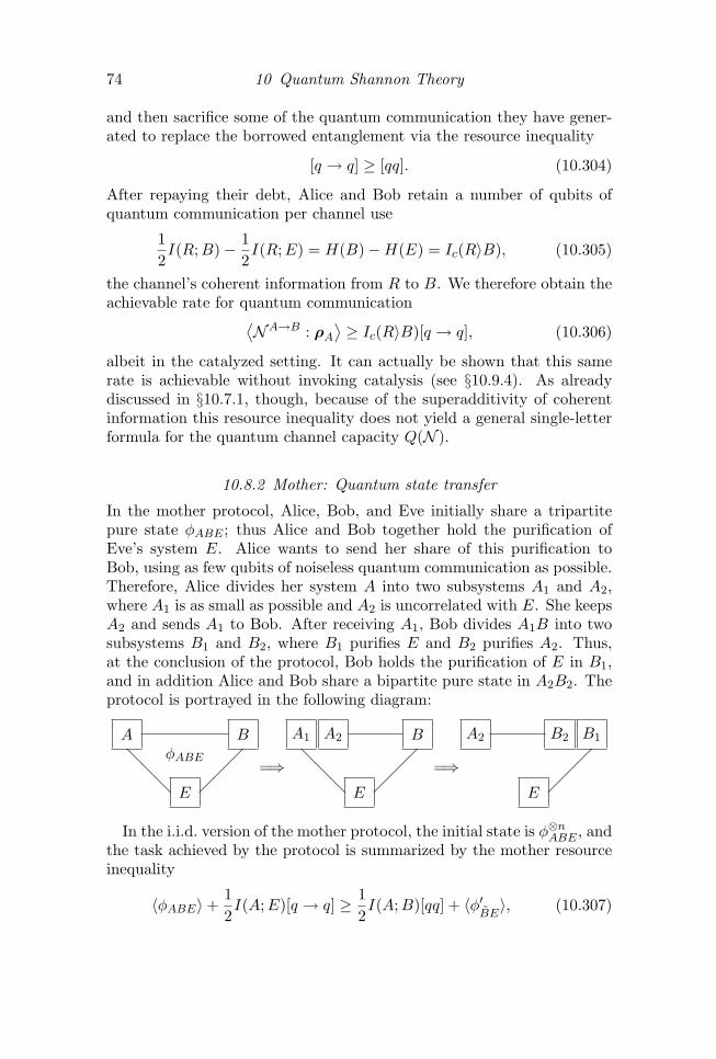
74 10 Quantum Shannon Theory
and then sacrifice some of the quantum communication they have gener-ated to replace the borrowed entanglement via the resource inequality
[q → q] ≥ [qq]. (10.304)
After repaying their debt, Alice and Bob retain a number of qubits ofquantum communication per channel use
12I(R;B)− 1
2I(R;E) = H(B)−H(E) = Ic(R〉B), (10.305)
the channel’s coherent information from R to B. We therefore obtain theachievable rate for quantum communication⟨
NA→B : ρA⟩≥ Ic(R〉B)[q → q], (10.306)
albeit in the catalyzed setting. It can actually be shown that this samerate is achievable without invoking catalysis (see §10.9.4). As alreadydiscussed in §10.7.1, though, because of the superadditivity of coherentinformation this resource inequality does not yield a general single-letterformula for the quantum channel capacity Q(N ).
10.8.2 Mother: Quantum state transfer
In the mother protocol, Alice, Bob, and Eve initially share a tripartitepure state φABE ; thus Alice and Bob together hold the purification ofEve’s system E. Alice wants to send her share of this purification toBob, using as few qubits of noiseless quantum communication as possible.Therefore, Alice divides her system A into two subsystems A1 and A2,where A1 is as small as possible and A2 is uncorrelated with E. She keepsA2 and sends A1 to Bob. After receiving A1, Bob divides A1B into twosubsystems B1 and B2, where B1 purifies E and B2 purifies A2. Thus,at the conclusion of the protocol, Bob holds the purification of E in B1,and in addition Alice and Bob share a bipartite pure state in A2B2. Theprotocol is portrayed in the following diagram:
A
E
B
@@
@
φABE=⇒
A1 A2
E
B
@@
@
=⇒
A2
E
B2 B1
In the i.i.d. version of the mother protocol, the initial state is φ⊗nABE , andthe task achieved by the protocol is summarized by the mother resourceinequality
〈φABE〉+12I(A;E)[q → q] ≥ 1
2I(A;B)[qq] + 〈φ′
BE〉, (10.307)

10.8 Quantum Protocols 75
where the resources on the left-hand side can be used to achieve theresult on the right-hand side, in an asymptotic i.i.d. setting, and theentropic quantities are evaluated in the state φABE . That is, if A(n)
1
denotes the state Alice sends and A(n)2 denotes the state she keeps, then
for any positive ε, the state of A(n)2 En is ε-close in the L1 norm to a
product state, where log∣∣∣A(n)
1
∣∣∣ = n2 I(A;E)+o(n), while A(n)
2 B(n)2 contains
n2 I(A;B)−o(n) shared ebits of entanglement. Eq.(10.307) means that forany input pure state φABE there is a way to choose the subsystem A
(n)2
of the specified dimension such that A(n)2 and En are nearly uncorrelated
and the specified amount of entanglement is harvested in A(n)2 B
(n)2 .
The mother protocol is in a sense dual to the father protocol. Whilethe father protocol consumes entanglement to achieve quantum commu-nication, the mother protocol consumes quantum communication andharvests entanglement. For the mother, I(A;B) quantifies the correla-tion between Alice and Bob at the beginning of the protocol (somethinggood), and I(A;E) quantifies the noise in the initial shared entanglement(something bad). The mother protocol can also be viewed as a quantumgeneralization of the Slepian-Wolf distributed compression protocol dis-cussed in §10.1.3. The mother protocol merges Alice’s and Bob’s sharesof the purification of E by sending Alice’s share to Bob, much as dis-tributed source coding merges the classical correlations shared by Aliceand Bob by sending Alice’s classical information to Bob. For this rea-son the mother protocol has been called the fully quantum Slepian-Wolfprotocol; the modifier “fully” will be clarified in §10.8.2, when we discussa variant on quantum state transfer in which classical communication isassumed to be freely available.
We may also view the mother protocol as a generalization of the en-tanglement concentration protocol discussed in §10.4, extending that dis-cussion in three ways:
1. The initial entangled state shared by Alice and Bob may be mixedrather than pure.
2. The communication from Alice to Bob is quantum rather than clas-sical.
3. The amount of communication that suffices to execute the protocolis quantified by the resource inequality.
Also note that if the state of AE is pure (uncorrelated with B), thenthe mother protocol reduces to Schumacher compression. In that case12I(A;E) = H(A), and the mother resource inequality states that the

76 10 Quantum Shannon Theory
purification of An can be transferred to Bob with high fidelity usingnH(A) + o(n) qubits of quantum communication.
Before proving the mother resource inequality, we will first discuss afew of its interesting consequences.
Hashing inequality. Suppose Alice and Bob wish to distill entanglementfrom many copies of the state φABE , using only local operations and clas-sical communication (LOCC). In the catalytic setting, they can borrowsome quantum communication, use the mother protocol to distill someshared entanglement, and then use classical communication and theirharvested entanglement to repay their debt via quantum teleportation.Using the teleportation resource inequality
TP : [qq] + 2[c→ c] ≥ [q → q] (10.308)
n2 I(A;E) times, and combining with the mother resource inequality, weobtain
〈φABE〉+ I(A;E)[c→ c] ≥ Ic(A〉B)[qq] + 〈φ′BE〉, (10.309)
since the net amount of distilled entanglement is 12I(A;B) per copy of
φ achieved by the mother minus the 12I(A;E) per copy consumed by
teleportation, and
12I(A;B)− 1
2I(A;E) = H(B)−H(E) = Ic(A〉B). (10.310)
Eq.(10.309) is the hashing inequality, which quantifies an achievable ratefor distilling ebits of entanglement shared by Alice and Bob from manycopies of a mixed state ρAB, using one-way classical communication, as-suming that Ic(A〉B) = −H(A|B) is positive. Furthermore, the hashinginequality tells us how much classical communication suffices for this pur-pose.
In the case where the state ρAB is pure, Ic(A〉B) = H(A)−H(AB) =H(A) and there is no environment E; thus we recover our earlier con-clusion about concentration of pure-state bipartite entanglement — thatH(A) Bell pairs can be extracted per copy, with a negligible classicalcommunication cost.
State merging. Suppose Alice and Bob share the purification of Eve’sstate, and Alice wants to transfer her share of the purification to Bob,where now unlimited classical communication from Alice to Bob is avail-able at no cost. In contrast to the mother protocol, Alice wants to achievethe transfer with as little one-way quantum communication as possible,even if she needs to send more bits in order to send fewer qubits.
10.8 Quantum Protocols 77
In the catalytic setting, Alice and Bob can borrow some quantum com-munication, perform the mother protocol, then use teleportation and theentanglement extracted by the mother protocol to repay some of the bor-rowed quantum communication. Combining teleportation of n
2 I(A;B)qubits with the mother resource inequality, we obtain
〈φABE〉+H(A|B)[q → q] + I(A;B)[c→ c] ≥ 〈φ′BE〉, (10.311)
using
12I(A;E)− 1
2I(A;B) = H(E)−H(B) = H(AB)−H(B) = H(A|B).
(10.312)
Eq.(10.311) is the state-merging inequality, expressing how much quantumand classical communication suffices to achieve the state transfer in ani.i.d. setting, assuming that H(A|B) is nonnegative.
Like the mother protocol, this state merging protocol can be viewed asa (partially) quantum version of the Slepian-Wolf protocol for mergingclassical correlations. In the classical setting, H(X|Y ) quantifies Bob’sremaining ignorance about Alice’s information X when Bob knows onlyY ; correspondingly, Alice can revealX to Bob by sendingH(X|Y ) bits perletter of X. Similarly, state merging provides an operational meaning tothe quantum conditional informationH(A|B), as the number of qubits percopy of φ that Alice sends to Bob to convey her share of the purification ofE, assuming classical communication is free. In this sense we may regardH(A|B) as a measure of Bob’s remaining “ignorance” about the sharedpurification of E when he holds only B.
Classically, H(X|Y ) is nonnegative, and zero if and only if Bob is al-ready certain about XY , but quantumly H(A|B) can be negative. Howcan Bob have “negative uncertainty” about the quantum state of AB?If H(A|B) < 0, or equivalently if I(A;E) < I(A;B), then the motherprotocol yields more quantum entanglement than the amount of quan-tum communication it consumes. Therefore, when H(A|B) is negative(i.e. Ic(A〉B) is positive), the mother resource inequality implies theHashing inequality, asserting that classical communication from Alice toBob not only achieves state transfer, but also distills −H(A|B) ebits ofentanglement per copy of φ. These distilled ebits can be deposited inthe entanglement bank, to be withdrawn as needed in future rounds ofstate merging, thus reducing the quantum communication cost of thosefuture rounds. Bob’s “negative uncertainty” today reduces the quantumcommunication cost of tasks to be performed tomorrow.

78 10 Quantum Shannon Theory
10.8.3 Operational meaning of strong subadditivity
The observation that H(A|B) is the quantum communication cost of statemerging allows us to formulate a simple operational proof of the strongsubadditivity of Von Neumann entropy, expressed in the form
H(A|BC) ≤ H(A|B), or −H(A|B) ≤ −H(A|BC). (10.313)
When H(A|B) is positive, eq.(10.313) is the obvious statement that it isno harder to merge Alice’s system with Bob’s if Bob holds C as well asB. When H(A|B) is negative, eq.(10.313) is the obvious statement thatAlice and Bob can distill no less entanglement using one-way classicalcommunication if Bob holds C as well as B.
To complete this argument, we need to know that H(A|B) is not onlyachievable but also that it is the optimal quantum communication costof state merging, and that −H(A|B) ebits is the optimal yield of hash-ing. The optimality follows from the principle that, for a bipartite purestate, k qubits of quantum communication cannot increase the sharedentanglement of AB by more than k ebits.
If H(A|B) is negative, consider cutting the system ABE into the twoparts AE and B, as in the following figure:
A
E
B
@@
@
@@
@@
@
@@
@@
@
=⇒
A2
E
B2 B1
@@
@@
@
@@
@@
@
In the hashing protocol, applied to n copies of φABE , the entanglementacross this cut at the beginning of the protocol is nH(B). By the end ofthe protocol En has decoupled from A
(n)2 and has entanglement nH(E)
with B(n)1 , ignoring o(n) corrections. If k ebits shared by Alice and Bob
are distilled, the final entanglement across the AE-B cut is
nH(E) + k ≤ nH(B) =⇒ k
n≤ H(B)−H(E) = −H(A|B). (10.314)
This inequality holds because LOCC cannot increase the entanglementacross the cut, and implies that no more than −H(A|B) ebits of en-tanglement per copy of φABE can be distilled in the hashing protocol,asymptotically.
On the other hand, if H(A|B) is positive, at the conclusion of statemerging B(n)
1 is entangled with En, and the entanglement across the AE-B cut is at least nH(E). To achieve this increase in entanglement, the

10.8 Quantum Protocols 79
number of qubits sent from Alice to Bob must be at least
k ≥ nH(E)− nH(B) =⇒ k
n≥ H(E)−H(B) = H(A|B) (10.315)
This inequality holds because the entanglement across the cut cannotincrease by more than the quantum communication across the cut, andimplies that at least H(A|B) qubits must be sent per copy of φABE toachieve state merging.
To summarize, we have proven strong subadditivity, not by the tradi-tional route of sophisticated matrix analysis, but via a less direct method.This proof is built on two cornerstones of quantum information theory —the decoupling principle and the theory of typical subspaces — which areessential ingredients in the proof of the mother resource inequality.
10.8.4 Negative conditional entropy in thermodynamics
As a further application of the decoupling mother resource inequality, wenow revisit Landauer’s Principle, developing another perspective on theimplications of negative quantum conditional entropy. Recall that erasureof a bit is a process which maps the bit to 0 irrespective of its initial value.This process is irreversible — knowing only the final state 0 after erasure,we cannot determine whether the initial state before erasure was 0 or 1.Irreversibility implies that erasure incurs an unavoidable thermodynamiccost. According to Landauer’s Principle, erasing a bit at temperature Trequires work no less than W = kT ln 2.
A specific erasure procedure is analyzed in Exercise 10.14. Suppose atwo-level quantum system has energy eigenstates |0〉, |1〉 with correspond-ing eigenvalues E0 and E1, where E = E1 − E0 ≥ 0. Initially the qubitis in an unknown mixture of these two states, and the energy splittingis E = 0. We erase the bit in three steps. In the first step, we bringthe bit into contact with a heat bath at temperature T > 0, and waitfor the bit to come to thermal equilibrium with the bath. In this stepthe bit “forgets” its initial value, but the bit is not yet erased becauseit has not been reset. In the second step, with the bit still in contactwith the bath, we turn on a control field which slowly increases E1 to avalue much larger than kT while maintaining thermal equilibrium all thewhile, thus resetting the bit to |0〉. In the third step, we isolate the bitfrom the bath and turn off the control field, so the two states of the bitbecome degenerate again. As shown in Exercise 10.14, work W = kT ln 2is required to execute step 2, with the energy dissipated as heat flowingfrom bit to bath.
We can also run the last two steps backward, increasing E1 while thebit is isolated from the bath, then decreasing E1 with the bit in contact

80 10 Quantum Shannon Theory
with the bath. This procedure maps the state |0〉 to the maximally mixedstate of the bit, extracting work W = kT ln 2 from the bath in the process.
Erasure is irreversible because the agent performing the erasure doesnot know the information being erased. (If a copy of the information werestored in her memory, survival of that copy would mean that the erasurehad not succeeded). From an information-theoretic perspective, the re-duction in the thermodynamic entropy of the erased bit, and hence thework required to perform the erasure, arises because erasure reduces theagent’s ignorance about the state of the bit, ignorance which is quantifiedby the Shannon entropy. But to be more precise, it is the conditional en-tropy of the system, given the state of the agent’s memory, which capturesthe agent’s ignorance before erasure and therefore also the thermodynamiccost of erasing. Thus the minimal work needed to erase system A shouldbe expressed as
W (A|O) = H(A|O)kT ln 2, (10.316)
where O is the memory of the observer who performs the erasure, andH(A|O) quantifies that observer’s ignorance about the state of A.
But what if A and O are quantum systems? We know that if A andO are entangled, then the conditional entropy H(A|O) can be negative.Does that mean we can erase A while extracting work rather than doingwork?
Yes, we can! Suppose for example that A and O are qubits and theirinitial state is maximally entangled. By controlling the contact betweenAO and the heat bath, the observer can extract work W = 2kT log 2while transforming AO to a maximally mixed state, using the same workextraction protocol as described above. Then she can do work W =kT log 2 to return A to the state |0〉. The net effect is to erase A whileextracting work W = kT log 2, satisfying the equality eq.(10.316).
To appreciate why this trick works, we should consider the joint stateof AO rather than the state of A alone. Although the marginal state of Ais mixed at the beginning of the protocol and pure at the end, the stateof AO is pure at the beginning and mixed at the end. Positive work isextracted by sacrificing the purity of AO.
To generalize this idea, let’s consider n 1 copies of the state ρAO ofsystem A and memory O. Our goal is to map the n copies of A to theerased state |000 . . . 0〉 while using or extracting the optimal amount ofwork. In fact, the optimal work per copy is given by eq.(10.316) in then→∞ limit.
To achieve this asymptotic work per copy, the observer first projectsAn onto its typical subspace, succeeding with probability 1 − o(1). Aunitary transformation then rotates the typical subspace to a subsystem
10.9 The Decoupling Inequality 81
A containing n(H(A) + o(1)) qubits, while erasing the complementaryqubits as in eq.(10.144). Now it only remains to erase A.
The mother resource inequality ensures that we may decompose A intosubsystems A1A2 such that A2 contains n
2 (I(A;O)− o(1)) qubits and isnearly maximally entangled with a subsystem of On. What is importantfor the erasure protocol is that we may identify a subsystem of AOn
containing n (I(A;O)− o(1)) qubits which is only distance o(1) away froma pure state. By controlling the contact between this subsystem and theheat bath, we may extract work W = n(I(A;O) − o(1))kT log 2 whiletransforming the subsystem to a maximally mixed state. We then proceedto erase A, expending work kT log |A| = n(H(A)+o(1))kT log 2. The network cost of the erasure, per copy of ρAO, is therefore
W = (H(A)− I(A;O) + o(1)) kT log 2 = (H(A|O) + o(1)) kT log 2,(10.317)
and the erasure succeeds with probability 1 − o(1). A notable feature ofthe protocol is that only the subsystem of On which is entangled with A2
is affected. Any correlation of the memory O with other systems remainsintact, and can be exploited in the future to reduce the cost of erasure ofthose other systems.
As does the state merging protocol, this erasure protocol provides anoperational interpretation of strong subadditivity. For positive H(A|O),H(A|O) ≥ H(A|OO′) means that it is no harder to erase A if the observerhas access to both O and O′ than if she has access to O alone. For negativeH(A|O), −H(A|OO′) ≥ −H(A|O) means that we can extract at least asmuch work from AOO′ as from its subsystem AO.
To carry out this protocol and extract the optimal amount of workwhile erasing A, we need to know which subsystem of On provides thepurification of A2. The decoupling argument ensures that this subsystemexists, but does not provide a constructive method for finding it, andtherefore no concrete protocol for erasing at optimal cost. This quandaryis characteristic of Shannon theory; for example, Shannon’s noisy channelcoding theorem ensures the existence of a code that achieves the channelcapacity, but does not provide any explicit code construction.
10.9 The Decoupling Inequality
Achievable rates for quantum protocols are derived by using randomcodes, much as in classical Shannon theory. But this similarity betweenclassical and quantum Shannon theory is superficial — at a deeper con-ceptual level, quantum protocols differ substantially from classical ones.Indeed, the decoupling principle underlies many of the key findings of

82 10 Quantum Shannon Theory
quantum Shannon theory, providing a unifying theme that ties togethermany different results. In particular, the mother and father resource in-equalities, and hence all their descendants enumerated above, follow froman inequality that specifies a sufficient condition for decoupling.
This decoupling inequality addresses the following question: Supposethat Alice and Eve share a quantum state σAE , where A is an n-qubitsystem. This state may be mixed, but in general A and E are correlated;that is, I(A;E) > 0. Now Alice starts discarding qubits one at a time,where each qubit is a randomly selected two-dimensional subsystem ofwhat Alice holds. Each time Alice discards a qubit, her correlation with Egrows weaker. How many qubits should she discard so that the subsystemshe retains has a negligible correlation with Eve’s system E?
To make the question precise, we need to formalize what it means todiscard a random qubit. More generally, suppose that A has dimension|A|, and Alice decomposes A into subsystems A1 and A2, then discards A1
and retains A2. We would like to consider many possible ways of choosingthe discarded system with specified dimension |A1|. Equivalently, we mayconsider a fixed decomposition A = A1A2, where we apply a unitarytransformation U to A before discarding A1. Then discarding a randomsubsystem with dimension |A1| is the same thing as applying a randomunitary U before discarding the fixed subsystem A1:
σAE@
@ E
A
UA1
A2
To analyze the consequences of discarding a random subsystem, then,we will need to be able to compute the expectation value of a functionf(U) when we average U uniformly over the group of unitary |A| × |A|matrices. We denote this expectation value as EU [f(U)]; to performcomputations we will only need to know that EU is suitably normalized,and is invariant under left or right multiplication by any constant unitarymatrix V :
EU [I] = 1, EU [f(U)] = EU [f(V U)] = EU [f(UV )] . (10.318)
These conditions uniquely define EU [f(U)], which is sometimes describedas the integral over the unitary group using the invariant measure or Haarmeasure on the group.
If we apply the unitary transformation U to A, and then discard A1,the marginal state of A2E is
σA2E(U) := trA1
((UA ⊗ IE) σAE
(U †A ⊗ IE
)). (10.319)
10.9 The Decoupling Inequality 83
The decoupling inequality expresses how close (in the L1 norm) σA2E isto a product state when we average over U :(
EU
[‖σA2E(U)− σmax
A2⊗ σE‖1
])2 ≤ |A2| · |E||A1|
tr(σ2AE
), (10.320)
where
σmaxA2
:=1|A2|
I (10.321)
denotes the maximally mixed state on A2, and σE is the marginal statetrAσAE .
This inequality has interesting consequences even in the case wherethere is no system E at all and σA is pure, where it becomes(
EU
[‖σA2(U)− σmax
A2‖1])2 ≤ |A2|
|A1|tr(σ2A
)=|A2||A1|
. (10.322)
Eq.(10.322) implies that, for a randomly chosen pure state of the bipartitesystem A = A1A2, where |A2|/|A1| 1, the density operator on A2 isvery nearly maximally mixed with high probability. One can likewiseshow that the expectation value of the entanglement entropy of A1A2 isvery close to the maximal value: E [H(A2)] ≥ log2 |A2|−|A2|/ (2|A1| ln 2).Thus, if for example A2 is 50 qubits and A1 is 100 qubits, the typicalentropy deviates from maximal by only about 2−50 ≈ 10−15.
10.9.1 Proof of the decoupling inequality
To prove the decoupling inequality, we will first bound the distance be-tween σA2E and a product state in the L2 norm, and then use the Cauchy-Schwarz inequality to obtain a bound on the L1 distance. Eq.(10.320)follows from
EU
[‖σA2E(U)− σmax
A2⊗ σE‖22
]≤ 1|A1|
tr(σ2AE
), (10.323)
combined with
(E [f ])2 ≤ E [f ]2 and ‖M‖21 ≤ d‖M‖22 (10.324)
(for nonnegative f), which implies
(E [‖ · ‖1])2 ≤ E[‖ · ‖21
]≤ |A2| · |E| · E
[‖ · ‖22
]. (10.325)
We also note that
‖σA2E − σmaxA2
⊗ σE‖22 = tr(σA2E − σmax
A2⊗ σE
)2= tr
(σ2A2E
)− 1|A2|
tr(σ2E
), (10.326)
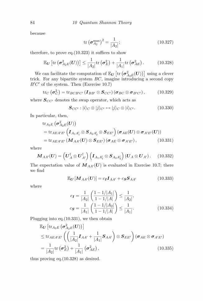
84 10 Quantum Shannon Theory
because
tr(σmaxA2
)2 =1|A2|
; (10.327)
therefore, to prove eq.(10.323) it suffices to show
EU
[tr(σ2A2E(U)
)]≤ 1|A2|
tr(σ2E
)+
1|A1|
tr(σ2AE
). (10.328)
We can facilitate the computation of EU
[tr(σ2A2E
(U))]
using a clevertrick. For any bipartite system BC, imagine introducing a second copyB′C ′ of the system. Then (Exercise 10.7)
trC(σ2C
)= trBCB′C′ (IBB′ ⊗ SCC′) (σBC ⊗ σB′C′) , (10.329)
where SCC′ denotes the swap operator, which acts as
SCC′ : |i〉C ⊗ |j〉C′ 7→ |j〉C ⊗ |i〉C′ . (10.330)
In particular, then,
trA2E
(σ2A2E(U)
)= trAEA′E′
(IA1A′1
⊗ SA2A′2⊗ SEE′
)(σAE(U)⊗ σA′E′(U))
= trAEA′E′ (MAA′(U)⊗ SEE′) (σAE ⊗ σA′E′) , (10.331)
where
MAA′(U) =(U †A ⊗U †
A′
)(IA1A′1
⊗ SA2A′2
)(UA ⊗UA′) . (10.332)
The expectation value of MAA′(U) is evaluated in Exercise 10.7; therewe find
EU [MAA′(U)] = cIIAA′ + cSSAA′ (10.333)
where
cI =1|A2|
(1− 1/|A1|1− 1/|A|
)≤ 1|A2|
,
cS =1|A1|
(1− 1/|A2|1− 1/|A|
)≤ 1|A1|
. (10.334)
Plugging into eq.(10.331), we then obtain
EU
[trA2E
(σ2A2E(U)
)]≤ trAEA′E′
((1|A2|
IAA′ +1|A1|
SAA′
)⊗ SEE′
)(σAE ⊗ σA′E′)
=1|A2|
tr(σ2E
)+
1|A1|
(σ2AE
), (10.335)
thus proving eq.(10.328) as desired.

10.9 The Decoupling Inequality 85
10.9.2 Proof of the mother inequality
The mother inequality eq.(10.307) follows from the decoupling inequalityeq.(10.320) in an i.i.d. setting. Suppose Alice, Bob, and Eve share thepure state φ⊗nABE . Then there are jointly typical subspaces of An, Bn, andEn, which we denote by A, B, E, such that∣∣A∣∣ = 2nH(A)+o(n),
∣∣B∣∣ = 2nH(B)+o(n),∣∣E∣∣ = 2nH(E)+o(n). (10.336)
Furthermore, the normalized pure state φ′ABE
obtained by projectingφ⊗nABE onto A ⊗ B ⊗ E deviates from φ⊗nABE by distance o(1) in the L1
norm.In order to transfer the purification of En to Bob, Alice first projects
An onto its typical subspace, succeeding with probability 1 − o(1), andcompresses the result. She then divides her compressed system A intotwo parts A1A2, and applies a random unitary to A before sending A1 toBob. Quantum state transfer is achieved if A2 decouples from E.
Because φ′ABE
is close to φ⊗nABE , we can analyze whether the protocolis successful by supposing the initial state is φ′
ABErather than φ⊗nABE .
According to the decoupling inequality(EU
[‖σA2E(U)− σmax
A2⊗ σE‖1
])2≤ |A| · |E|
|A1|2tr(σ2AE
)=
1|A1|2
2n(H(A)+H(E)+o(1)) tr(σ2AE
)=
1|A1|2
2n(H(A)+H(E)−H(B)+o(1));
(10.337)
here we have used properties of typical subspaces in the second line, aswell as the property that σAE and σB have the same nonzero eigenvalues,because φ′
ABEis pure.
Eq.(10.337) bounds the L1 distance of σA2E(U) from a product statewhen averaged over all unitaries, and therefore suffices to ensure the exis-tence of at least one unitary transformation U such that the L1 distanceis bounded above by the right-hand side. Therefore, by choosing thisU , Alice can decouple A2 from En to o(1) accuracy in the L1 norm bysending to Bob
log2 |A1| =n
2(H(A) +H(E)−H(B) + o(1)) =
n
2(I(A;E) + o(1))
(10.338)
qubits, randomly chosen from the (compressed) typical subspace of An.Alice retains nH(A)− n
2 I(A;E)− o(n) qubits of her compressed system,which are nearly maximally mixed and uncorrelated with En; hence atthe end of the protocol she shares with Bob this many qubit pairs, which

86 10 Quantum Shannon Theory
have high fidelity with a maximally entangled state. Since φABE is pure,and therefore H(A) = 1
2 (I(A;E)− I(A;B)), we conclude that Alice andBob distill n2 I(A;B)−o(n) ebits of entanglement, thus proving the motherresource inequality.
We can check that this conclusion is plausible using a crude countingargument. Disregarding the o(n) corrections in the exponent, the stateφ⊗nABE is nearly maximally mixed on a typical subspace of AnEn withdimension 2nH(AE), i.e. the marginal state on AE can be realized as anearly uniform ensemble of this many mutually orthogonal states. If A1
is randomly chosen and sufficiently small, we expect that, for each statein this ensemble, A1 is nearly maximally entangled with a subsystemof the much larger system A2E, and that the marginal states on A2Earising from different states in the AE ensemble have a small overlap.Therefore, we anticipate that tracing out A1 yields a state on A2E whichis nearly maximally mixed on a subspace with dimension |A1|2nH(AE).Approximate decoupling occurs when this state attains full rank on A2E,since in that case it is close to maximally mixed on A2E and thereforeclose to a product state on its support. The state transfer succeeds,therefore, provided
|A1|2nH(AE) ≈ |A2| · |E| =|A| · |E||A1|
≈ 2n(H(A)+H(E))
|A1|=⇒ |A1|2 ≈ 2nI(A;E), (10.339)
as in eq.(10.338).Our derivation of the mother resource inequality, based on random cod-
ing, does not exhibit any concrete protocol that achieves the claimed rate,nor does it guarantee the existence of any protocol in which the requiredquantum processing can be executed efficiently. Concerning the latterpoint, it is notable that our derivation of the decoupling inequality ap-plies not just to the expectation value averaged uniformly over the unitarygroup, but also to any average over unitary transformations which satisfieseq.(10.333). In fact, this identity is satisfied by a uniform average over theClifford group, which means that there is some Clifford transformationon A which achieves the rates specified in the mother resource inequality.Any Clifford transformation on n qubits can be reached by a circuit withO(n2) gates. Since it is also known that Schumacher compression can beachieved by a polynomial-time quantum computation, Alice’s encodingoperation can be carried out efficiently.
In fact, after compressing, Alice encodes the quantum information shesends to Bob using a stabilizer code (with Clifford encoder U), and Bob’stask, after receiving A1 is to correct the erasure of A2. Bob can replaceeach erased qubit by the standard state |0〉 , and then measure the code’s

10.9 The Decoupling Inequality 87
check operators. With high probability, there is a unique Pauli operatoracting on the erased qubits that restores Bob’s state to the code space, andthe recovery operation can be efficiently computed using linear algebra.Hence, Bob’s part of the mother protocol, like Alice’s, can be executedefficiently.
10.9.3 Proof of the father inequality
One-shot version. In the one-shot version of the father protocol, Alice andBob share a pair of maximally entangled systems A1B1, and in additionAlice holds input state ρA2
of system A2 which she wants to conveyto Bob. Alice encodes ρA2
by applying a unitary transformation V toA = A1A2, then sends A to Bob via the noisy quantum channel NA→B2 .Bob applies a decoding map DB1B2→A2 jointly to the channel output andhis half of the entangled state he shares with Alice, hoping to recoverAlice’s input state with high fidelity:
A1
B1
A2
@@
V A N B2
D A2
We would like to know how much shared entanglement suffices for Aliceand Bob to succeed.
This question can be answered using the decoupling inequality. Firstwe introduce a reference system R′ which is maximally entangled withA2; then Bob succeeds if his decoder can extract the purification of R′.Because the systems R′B1 and A1A1 are maximally entangled, the encod-ing unitary V acting on A1A2 can be replaced by its transpose V T actingon R′B1. We may also replace N by its Stinespring dilation UA1A2→B2E ,so that the extended output state φ of R′B1B2E is pure:
A1
B1
A2
R′
@@
@@
@@
V UB2
E
=@
@@
@
A1
B1
A2
R′
@@
@@
@@
V T
UB2
E

88 10 Quantum Shannon Theory
Finally we invoke the decoupling principle — if R′ and E decouple, thenR′ is purified by a subsystem of B1B2, which means that Bob can recoverρA2
with a suitable decoding map.If we consider V , and hence also V T , to be a random unitary, then
we may describe the situation this way: We have a tripartite pure stateφRB2E , where R = R′B1, and we would like to know whether the marginalstate of R′E is close to a product state when the random subsystemB1 is discarded from R. This is exactly the question addressed by thedecoupling inequality, which in this case may be expressed as(
EV
[‖σR′E(V )− σmax
R′ ⊗ σE‖1])2 ≤ |R| · |E|
|B1|2tr(σ2RE
), (10.340)
Eq.(10.340) asserts that the L1 distance from a product state is boundedabove when averaged uniformly over all unitary V ’s; therefore there mustbe some particular encoding unitary V that satisfies the same bound. Weconclude that near-perfect decoupling of R′E, and therefore high-fidelitydecoding of B2, is achievable provided that
|A1| = |B1| |R′| · |E| tr(σ2RE
)= |A2| · |E| tr
(σ2B2
), (10.341)
where to obtain the second equality we use the purity of φRB2E and recallthat the reference system R′ is maximally entangled with A2.
i.i.d. version. In the i.i.d. version of the father protocol, Alice andBob achieve high fidelity entanglement-assisted quantum communicationthrough n uses of the quantum channel NA→B. The code they use forthis purpose can be described in the following way: Consider an inputdensity operator ρA of system A, which is purified by a reference systemR. Sending the purified input state ψRA through UA→BE , the isometricdilation of NA→B, generates the tripartite pure state φRBE . Evidentlyapplying
(UA→BE
)⊗n to ψ⊗nRA produces φ⊗nRBE .But now suppose that before transmitting the state to Bob, Alice
projects An onto its typical subspace A, succeeding with probability1 − o(1) in preparing a state of AR that is nearly maximally entangled,where R is the typical subspace of Rn. Imagine dividing R into a ran-domly chosen subsystem B1 and its complementary subsystem R′; thenthere is a corresponding decomposition of A = A1A2 such that A1 is verynearly maximally entangled with B1 and A2 is very nearly maximallyentangled with R′.
If we interpret B1 as Bob’s half of an entangled state of A1B1 sharedwith Alice, this becomes the setting where the one-shot father protocolapplies, if we ignore the small deviation from maximal entanglement inA1B1 and R′A2. As for our analysis of the i.i.d. mother protocol, we apply

10.9 The Decoupling Inequality 89
the one-shot father inequality not to φ⊗nRBE , but rather to the nearby stateφ′RBE
, where B and E are the typical subspaces of Bn and En respec-tively. Applying eq.(10.340), and using properties of typical subspaces,we can bound the square of the L1 deviation of R′E from a product state,averaged over the choice of B1, by
|R| · |E||B1|2
tr(σ2B
)=
2n(H(R)+H(E)−H(B)+o(1))
|B1|2=
2n(I(R;E)+o(1))
|B1|2; (10.342)
hence the bound also applies for some particular way of choosing B1.This choice defines the code used by Alice and Bob in a protocol whichconsumes
log2 |B1| =n
2I(R;E) + o(n) (10.343)
ebits of entanglement, and conveys from Alice to Bob
nH(B)− n
2I(R;E)− o(n) =
n
2I(R;B)− o(n) (10.344)
high-fidelity qubits. This proves the father resource inequality.
10.9.4 Quantum channel capacity revisited
In §10.8.1 we showed that the coherent information is an achievable ratefor quantum communication over a noisy quantum channel. That deriva-tion, a corollary of the father resource inequality, applied to a catalyticsetting, in which shared entanglement between sender and receiver canbe borrowed and later repaid. It is useful to see that the same rate isachievable without catalysis, a result we can derive from an alternativeversion of the decoupling inequality.
This version applies to the setting depicted here:
ψRA@
@
R
A
V
U
|0〉R2
BE
A density operator ρA for system A, with purification ψRA, is transmit-ted through a channel NA→B which has the isometric dilation UA→BE .The reference system R has a decomposition into subsystems R1R2. Weapply a random unitary transformation V to R, then project R1 onto afixed vector |0〉R1 , and renormalize the resulting state. In effect, then weare projecting R onto a subspace with dimension |R2|, which purifies a

90 10 Quantum Shannon Theory
corresponding code subspace of A. This procedure prepares a normalizedpure state φR2BE , and a corresponding normalized marginal state σR2E
of R2E.If R2 decouples from E, then R2 is purified by a subsystem of B, which
means that the code subspace of A can be recovered by a decoder appliedto B. A sufficient condition for approximate decoupling can be derivedfrom the inequality(
EV
[‖σR2E(V )− σmax
R2⊗ σE‖1
])2 ≤ |R2| · |E| tr(σ2RE
). (10.345)
Eq.(10.345) resembles eq.(10.320) and can be derived by a similar method.Note that the right-hand side of eq.(10.345) is enhanced by a factor of|R1| relative to the right-hand side of eq.(10.320). This factor arises be-cause after projecting R1 onto the fixed state |0〉 we need to renormalizethe state by multiplying by |R1|, while on the other hand the projectionsuppresses the expected distance squared from a product state by a factor|R1|.
In the i.i.d. setting where the noisy channel is used n times, we considerφ⊗nRBE , and project onto the jointly typical subspaces R, B, E of Rn, Bn,En respectively, succeeding with high probability. We choose a code byprojecting R onto a random subspace with dimension |R2|. Then, theright-hand side of eq.(10.345) becomes
|R2| · 2n(H(E)−H(B)+o(1)), (10.346)
and since the inequality holds when we average uniformly over V , it surelyholds for some particular V . That unitary defines a code which achievesdecoupling and has the rate
1n
log2 |R2| = H(E)−H(B)− o(1) = Ic(R〉B)− o(1). (10.347)
Hence the coherent information is an achievable rate for high-fidelityquantum communication over the noisy channel.
10.9.5 Black holes as mirrors
As our final application of the decoupling inequality, we consider a highlyidealized model of black hole dynamics. Suppose that Alice holds a k-qubit system A which she wants to conceal from Bob. To be safe, shediscards her qubits by tossing them into a large black hole, where sheknows Bob will not dare to follow. The black hole B is an (n−k)-qubitsystem, which grows to n qubits after merging with A, where n is muchlarger than k.

10.9 The Decoupling Inequality 91
Black holes are not really completely black — they emit Hawking ra-diation. But qubits leak out of an evaporating black hole very slowly, ata rate per unit time which scales like n−1/2. Correspondingly, it takestime Θ(n3/2) for the black hole to radiate away a significant fraction ofits qubits. Because the black hole Hilbert space is so enormous, this isa very long time, about 1067 years for a solar mass black hole, for whichn ≈ 1078. Though Alice’s qubits might not remain secret forever, she iscontent knowing that they will be safe from Bob for 1067 years.
But in her haste, Alice fails to notice that her black hole is very, veryold. It has been evaporating for so long that it has already radiated awaymore than half of its qubits. Let’s assume that the joint state of the blackhole and its emitted radiation is pure, and furthermore that the radiationis a Haar-random subsystem of the full system.
Because the black hole B is so old, |B| is much smaller than the dimen-sion of the radiation subsystem; therefore, as in eq.(10.322), we expectthe state of B to be very nearly maximally mixed with high probability.We denote by RB the subsystem of the emitted radiation which purifiesB; thus the state of BRB is very nearly maximally entangled. We assumethat RB has been collected by Bob and is under his control.
To keep track of what happens to Alice’s k qubits, we suppose thather k-qubit system A is maximally entangled with a reference systemRA. After A enters the black hole, Bob waits for a while, until the k′-qubit system A′ is emitted in the black hole’s Hawking radiation. Afterretrieving A′, Bob hopes to recover the purification of RA by applying asuitable decoding map to A′RB. Can he succeed?
We’ve learned that Bob can succeed with high fidelity if the remainingblack hole system B′ decouples from Alice’s reference system RA. Let’ssuppose that the qubits emitted in the Hawking radiation are chosenrandomly; that is, A′ is a Haar-random k′-qubit subsystem of the n-qubitsystem AB, as depicted here:
@@
RA
B′A
Alice
U
@@
@@@
B
RB
A′
Bob
The double lines indicate the very large systems B and B′, and singlelines the smaller systems A and A′. Because the radiated qubits are

92 10 Quantum Shannon Theory
random, we can determine whether RAB′ decouples using the decouplinginequality, which for this case becomes
EU
[‖σB′RA
(U)− σmaxB′ ⊗ σRA
‖1]≤
√|ABRA||A′|2
tr(σ2ABRA
).
(10.348)
Because the state of ARA is pure, and B is maximally entangled withRB, we have tr
(σ2ABRA
)= 1/|B|, and therefore the Haar-averaged L1
distance of σB′RAfrom a product state is bounded above by√
|ARA||A′|2
=|A||A′|
. (10.349)
Thus, if Bob waits for only k′ = k + c qubits of Hawking radiation to beemitted after Alice tosses in her k qubits, Bob can decode her qubits withexcellent fidelity F ≥ 1− 2−c.
Alice made a serious mistake. Rather than waiting for Ω(n) qubits toemerge from the black hole, Bob can already decode Alice’s secret quitewell when he has collected just a few more than k qubits. And Bob isan excellent physicist, who knows enough about black hole dynamics toinfer the encoding unitary transformation U , information he uses to findthe right decoding map.
We could describe the conclusion, more prosaically, by saying thatthe random unitary U applied to AB encodes a good quantum error-correcting code, which achieves high-fidelity entanglement-assisted trans-mission of quantum information though an erasure channel with a higherasure probability. Of the n input qubits, only k′ randomly selectedqubits are received by Bob; the rest remain inside the black hole andhence are inaccessible. The input qubits, then, are erased with probabil-ity p = (n − k′)/n, while nearly error-free qubits are recovered from theinput qubits at a rate
R =k
n= 1− p− k′ − k
n; (10.350)
in the limit n→∞ with c = k′ − k fixed, this rate approaches 1− p, theentanglement-assisted quantum capacity of the erasure channel.
So far, we’ve assumed that the emitted system A′ is a randomly selectedsubsystem of AB. That won’t be true for a real black hole. However, it isbelieved that the internal dynamics of actually black holes mixes quantuminformation quite rapidly (the fast scrambling conjecture). For a blackhole with temperature T , it takes time of order ~/kT for each qubit to be

10.10 Summary 93
emitted in the Hawking radiation, and a time longer by only a factor oflog n for the dynamics to mix the black hole degrees of freedom sufficientlyfor our decoupling estimate to hold with reasonable accuracy. For a solarmass black hole, Alice’s qubits are revealed just a few milliseconds aftershe deposits them, much faster than the 1067 years she had hoped for!Because Bob holds the system RB which purifies B, and because he knowsthe right decoding map to apply to A′RB, the black hole behaves like aninformation mirror — Alice’s qubits bounce right back!
If Alice is more careful, she will dump her qubits into a young blackhole instead. If we assume that the initial black hole B is in a pure state,then σABRA
is also pure, and the Haar-averaged L1 distance of σB′RA
from a product state is bounded above by√|ABRA||A′|2
=2n+k
22k′=
12c
(10.351)
after
k′ =12(n+ k + c) (10.352)
qubits are emitted. In this case, Bob needs to wait a long time, until morethan half of the qubits in AB are radiated away. Once Bob has acquiredk + c more qubits than the number still residing in the black hole, heis empowered to decode Alice’s k qubits with fidelity F ≥ 1 − 2−c. Infact, there is nothing special about Alice’s subsystem A; by adjustinghis decoding map appropriately, Bob can decode any k qubits he choosesfrom among the n qubits in the initial black hole AB.
There is far more to learn about quantum information processing byblack holes, an active topic of current research (as of this writing in 2016),but we will not delve further into this fascinating topic here. We can beconfident, though, that the tools and concepts of quantum informationtheory discussed in this book will be helpful for addressing the manyunresolved mysteries of quantum gravity.
10.10 Summary
Shannon entropy and classical data compression. The Shannonentropy of an ensembleX = x, p(x) isH(X) ≡ 〈− log p(x)〉; it quantifiesthe compressibility of classical information. A message n letters long,where each letter is drawn independently from X, can be compressedto H(X) bits per letter (and no further), yet can still be decoded witharbitrarily good accuracy as n→∞.
Conditional entropy and information merging. The conditionalentropy H(X|Y ) = H(XY )−H(Y ) quantifies how much the information

94 10 Quantum Shannon Theory
source X can be compressed when Y is known. If n letters are drawnfrom XY , where Alice holds X and Bob holds Y , Alice can convey X toBob by sending H(X|Y ) bits per letter, asymptotically as n→∞.
Mutual information and classical channel capacity. The mutualinformation I(X;Y ) = H(X) +H(Y )−H(XY ) quantifies how informa-tion sources X and Y are correlated; when we learn the value of y weacquire (on the average) I(X;Y ) bits of information about x, and viceversa. The capacity of a memoryless noisy classical communication chan-nel is C = maxX I(X;Y ). This is the highest number of bits per letterthat can be transmitted through n uses of the channel, using the bestpossible code, with negligible error probability as n→∞.
Von Neumann entropy and quantum data compression. TheVon Neumann entropy of a density operator ρ is
H(ρ) = −trρ log ρ; (10.353)
it quantifies the compressibility of an ensemble of pure quantum states.A message n letters long, where each letter is drawn independently fromthe ensemble |ϕ(x)〉, p(x), can be compressed to H(ρ) qubits per letter(and no further) where ρ =
∑X p(x)|ϕ(x)〉〈ϕ(x)|, yet can still be decoded
with arbitrarily good fidelity as n→∞.Entanglement concentration and dilution. The entanglement E of
a bipartite pure state |ψ〉AB is E = H(ρA) where ρA = trB(|ψ〉〈ψ|). Withlocal operations and classical communication, we can prepare n copies of|ψ〉AB from nE Bell pairs (but not from fewer), and we can distill nE Bellpairs (but not more) from n copies of |ψ〉AB, asymptotically as n→∞.
Accessible information. The Holevo chi of an ensemble E =ρ(x), p(x) of quantum states is
χ(E) = H
(∑x
p(x)ρ(x)
)−∑x
p(x)H(ρ(x)). (10.354)
The accessible information of an ensemble E of quantum states is themaximal number of bits of information that can be acquired about thepreparation of the state (on the average) with the best possible measure-ment. The accessible information cannot exceed the Holevo chi of theensemble. The product-state capacity of a quantum channel N is
C1(N ) = maxE
χ(N (E)). (10.355)
This is the highest number of classical bits per letter that can be trans-mitted through n uses of the quantum channel, with negligible error prob-ability as n→∞, assuming that each codeword is a product state.

10.10 Summary 95
Decoupling and quantum communication. In a tripartite purestate φRBE , we say that systems R and E decouple if the marginal den-sity operator of RE is a product state, in which case R is purified bya subsystem of B. A quantum state transmitted through a noisy quan-tum channel NA→B (with isometric dilation UA→BE) can be accuratelydecoded if a reference system R which purifies channel’s input A nearlydecouples from the channel’s environment E.
Father and mother protocols. The father and mother resourceinequalities specify achievable rates for entanglement-assisted quantumcommunication and quantum state transfer, respectively. Both followfrom the decoupling inequality, which establishes a sufficient condition forapproximate decoupling in a tripartite mixed state. By combining the fa-ther and mother protocols with superdense coding and teleportation, wecan derive achievable rates for other protocols, including entanglement-assisted classical communication, quantum communication, entanglementdistillation, and quantum state merging.
Homage to Ben Schumacher:
Ben.He rocks.I rememberWhenHe showed me how to fitA qubitIn a small box.
I wonder how it feelsTo be compressed.And then to passA fidelity test.
Or does it feelAt all, and if it doesWould I squealOr be just as I was?
If not undoneI’d become as I’d begunAnd write a memorandumOn being random.Had it felt like a beltOf rum?
And might it be predictedThat I’d become addicted,

96 10 Quantum Shannon Theory
Longing for my sessionOf compression?
I’d crawlTo Ben again.And call,Put down your pen!Don’t stall!Make me small!
10.11 Bibliographical Notes
Cover and Thomas [2] is an excellent textbook on classical informationtheory. Shannon’s original paper [3] is still very much worth reading.
Nielsen and Chuang [4] provide a clear introduction to some aspectsof quantum Shannon theory. Wilde [1] is a more up-to-date and verythorough account.
Properties of entropy are reviewed in [5]. Strong subadditivity of VonNeumann entropy was proven by Lieb and Ruskai [6], and the conditionfor equality was derived by Hayden et al. [7]. The connection betweenseparability and majorization was pointed out by Nielsen and Kempe [8].
Bekenstein’s entropy bound was formulated in [9] and derived by Casini[10]. Entropic uncertainty relations are reviewed in [11], and I followtheir derivation. The original derivation, by Maassen and Uffink [12] usesdifferent methods.
Schumacher compression was first discussed in [13, 14], and Bennettet al. [15] devised protocols for entanglement concentration and dilution.Measures of mixed-state entanglement are reviewed in [16]. The reversibletheory of mixed-state entanglement was formulated by Brandao and Ple-nio [17]. Squashed entanglement was introduced by Christandl and Win-ter [18], and its monogamy discussed by Koashi and Winter [19]. Brandao,Christandl, and Yard [20] showed that squashed entanglement is positivefor any nonseparable bipartite state. Doherty, Parrilo, and Spedalieri [21]showed that every nonseparable bipartite state fails to be k-extendablefor some finite k.
The Holevo bound was derived in [22]. Peres-Wootters coding was dis-cussed in [23]. The product-state capacity formula was derived by Holevo[24] and by Schumacher and Westmoreland [25]. Hastings [26] showedthat Holevo chi can be superadditive. Horodecki, Shor, and Ruskai [27]introduced entanglement-breaking channels, and additivity of Holevo chifor these channels was shown by Shor [28].
Necessary and sufficient conditions for quantum error correction wereformulated in terms of the decoupling principle by Schumacher and

10.12 Exercises 97
Nielsen [29]; that (regularized) coherent information is an upper boundon quantum capacity was shown by Schumacher [30], Schumacher andNielsen [29], and Barnum et al. [31]. That coherent information is anachievable rate for quantum communication was conjectured by Lloyd[32] and by Schumacher [30], then proven by Shor [33] and by Devetak[34]. Devetak and Winter [35] showed it is also an achievable rate forentanglement distillation. The quantum Fano inequality was derived bySchumacher [30].
Approximate decoupling was analyzed by Schumacher and Westmore-land [36], and used to prove capacity theorems by Devetak [34], byHorodecki et al. [37], by Hayden et al. [38], and by Abeyesinghe etal. [39]. The entropy of Haar-random subsystems had been discussedearlier, by Lubkin [40], Lloyd and Pagels [41], and Page [42]. Devetak,Harrow, and Winter [43, 44] introduced the mother and father proto-cols and their descendants. Devatak and Shor [45] introduced degradablequantum channels and proved that coherent information is additive forthese channels. Bennett et al. [46, 47] found the single-letter formulafor entanglement-assisted classical capacity. Superadditivity of coherentinformation was discovered by Shor and Smolin [48] and by DiVincenzoet al. [49]. Smith and Yard [50] found extreme examples of superadditiv-ity, in which two zero-capacity channels have nonzero capacity when usedjointly. The achievable rate for state merging was derived by Horodecki etal. [37], and used by them to prove strong subadditivity of Von Neumannentropy.
Decoupling was applied to Landuaer’s principle by Renner et al. [51],and to black holes by Hayden and Preskill [52]. The fast scramblingconjecture was proposed by Sekino and Susskind [53].
10.12 Exercises
10.1 Positivity of quantum relative entropy
a) Show that lnx ≤ x − 1 for all positive real x, with equality iffx = 1.
b) The (classical) relative entropy of a probability distributionp(x) relative to q(x) is defined as
D(p ‖ q) ≡∑x
p(x) (log p(x)− log q(x)) . (10.356)
Show thatD(p ‖ q) ≥ 0 , (10.357)
with equality iff the probability distributions are identical.Hint: Apply the inequality from (a) to ln (q(x)/p(x)).

98 10 Quantum Shannon Theory
c) The quantum relative entropy of the density operator ρ withrespect to σ is defined as
D(ρ ‖ σ) = tr ρ (log ρ− log σ) . (10.358)
Let pi denote the eigenvalues of ρ and qa denote the eigen-values of σ. Show that
D(ρ ‖ σ) =∑i
pi
(log pi −
∑a
Dia log qa
), (10.359)
where Dia is a doubly stochastic matrix. Express Dia in termsof the eigenstates of ρ and σ. (A matrix is doubly stochastic ifits entries are nonnegative real numbers, where each row andeach column sums to one.)
d) Show that if Dia is doubly stochastic, then (for each i)
log
(∑a
Diaqa
)≥∑a
Dia log qa , (10.360)
with equality only if Dia = 1 for some a.e) Show that
D(ρ ‖ σ) ≥ D(p ‖ r) , (10.361)
where ri =∑
aDiaqa.f) Show that D(ρ ‖ σ) ≥ 0, with equality iff ρ = σ.
10.2 Properties of Von Neumann entropy
a) Use nonnegativity of quantum relative entropy to prove the sub-additivity of Von Neumann entropy
H(ρAB) ≤ H(ρA) +H(ρB), (10.362)
with equality iff ρAB = ρA ⊗ ρB. Hint: Consider the relativeentropy of ρAB and ρA ⊗ ρB.
b) Use subadditivity to prove the concavity of the Von Neumannentropy:
H(∑x
pxρx) ≥∑x
pxH(ρx) . (10.363)
Hint: Consider
ρAB =∑x
px (ρx)A ⊗ (|x〉〈x|)B , (10.364)
where the states |x〉B are mutually orthogonal.

10.12 Exercises 99
c) Use the condition
H(ρAB) = H(ρA) +H(ρB) iff ρAB = ρA ⊗ ρB (10.365)
to show that, if all px’s are nonzero,
H
(∑x
pxρx
)=∑x
pxH(ρx) (10.366)
iff all the ρx’s are identical.
10.3 Monotonicity of quantum relative entropy
Quantum relative entropy has a property called monotonicity:
D(ρA‖σA) ≤ D(ρAB‖σAB); (10.367)
The relative entropy of two density operators on a system AB can-not be less than the induced relative entropy on the subsystem A.
a) Use monotonicity of quantum relative entropy to prove thestrong subadditivity property of Von Neumann entropy. Hint:On a tripartite system ABC, consider the relative entropy ofρABC and ρA ⊗ ρBC .
b) Use monotonicity of quantum relative entropy to show that theaction of a quantum channel N cannot increase relative en-tropy:
D(N (ρ)‖N (σ) ≤ D(ρ‖σ), (10.368)
Hint: Recall that any quantum channel has an isometric dila-tion.
10.4 The Peres–Wootters POVM.
Consider the Peres–Wootters information source described in§10.6.4 of the lecture notes. It prepares one of the three states
|Φa〉 = |ϕa〉 ⊗ |ϕa〉, a = 1, 2, 3, (10.369)
each occurring with a priori probability 13 , where the |ϕa〉’s are
defined in eq.(10.214).
a) Express the density matrix
ρ =13
(∑a
|Φa〉〈Φa|
), (10.370)
in terms of the Bell basis of maximally entangled states|φ±〉, |ψ±〉, and compute H(ρ).

100 10 Quantum Shannon Theory
b) For the three vectors |Φa〉, a = 1, 2, 3, construct the “prettygood measurement” defined in eq.(10.227). (Again, expandthe |Φa〉’s in the Bell basis.) In this case, the PGM is anorthogonal measurement. Express the elements of the PGMbasis in terms of the Bell basis.
c) Compute the mutual information of the PGM outcome and thepreparation.
10.5 Separability and majorization
The hallmark of entanglement is that in an entangled state the wholeis less random than its parts. But in a separable state the correla-tions are essentially classical and so are expected to adhere to theclassical principle that the parts are less disordered than the whole.The objective of this problem is to make this expectation precise byshowing that if the bipartite (mixed) state ρAB is separable, then
λ(ρAB) ≺ λ(ρA) , λ(ρAB) ≺ λ(ρB) . (10.371)
Here λ(ρ) denotes the vector of eigenvalues of ρ, and ≺ denotesmajorization.A separable state can be realized as an ensemble of pure productstates, so that if ρAB is separable, it may be expressed as
ρAB =∑a
pa |ψa〉〈ψa| ⊗ |ϕa〉〈ϕa| . (10.372)
We can also diagonalize ρAB, expressing it as
ρAB =∑j
rj |ej〉〈ej | , (10.373)
where |ej〉 denotes an orthonormal basis for AB; then by the HJWtheorem, there is a unitary matrix V such that
√rj |ej〉 =
∑a
Vja√pa|ψa〉 ⊗ |ϕa〉 . (10.374)
Also note that ρA can be diagonalized, so that
ρA =∑a
pa|ψa〉〈ψa| =∑µ
sµ|fµ〉〈fµ| ; (10.375)
here |fµ〉 denotes an orthonormal basis for A, and by the HJWtheorem, there is a unitary matrix U such that
√pa|ψa〉 =
∑µ
Uaµ√sµ|fµ〉 . (10.376)
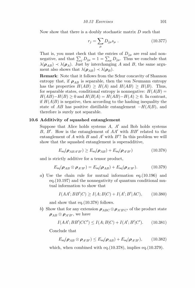
10.12 Exercises 101
Now show that there is a doubly stochastic matrix D such that
rj =∑µ
Djµsµ . (10.377)
That is, you must check that the entries of Djµ are real and non-negative, and that
∑j Djµ = 1 =
∑µDjµ. Thus we conclude that
λ(ρAB) ≺ λ(ρA). Just by interchanging A and B, the same argu-ment also shows that λ(ρAB) ≺ λ(ρB).Remark: Note that it follows from the Schur concavity of Shannonentropy that, if ρAB is separable, then the von Neumann entropyhas the properties H(AB) ≥ H(A) and H(AB) ≥ H(B). Thus,for separable states, conditional entropy is nonnegative: H(A|B) =H(AB)−H(B) ≥ 0 andH(B|A) = H(AB)−H(A) ≥ 0. In contrast,if H(A|B) is negative, then according to the hashing inequality thestate of AB has positive distillable entanglement −H(A|B), andtherefore is surely not separable.
10.6 Additivity of squashed entanglement
Suppose that Alice holds systems A, A′ and Bob holds systemsB, B′. How is the entanglement of AA′ with BB′ related to theentanglement of A with B and A′ with B′? In this problem we willshow that the squashed entanglement is superadditive,
Esq(ρABA′B′) ≥ Esq(ρAB) + Esq(ρA′B′) (10.378)
and is strictly additive for a tensor product,
Esq(ρAB ⊗ ρA′B′) = Esq(ρAB) + Esq(ρA′B′). (10.379)
a) Use the chain rule for mutual information eq.(10.196) andeq.(10.197) and the nonnegativity of quantum conditional mu-tual information to show that
I(AA′;BB′|C) ≥ I(A;B|C) + I(A′;B′|AC), (10.380)
and show that eq.(10.378) follows.b) Show that for any extension ρABC⊗ρA′B′C′ of the product state
ρAB ⊗ ρA′B′ , we have
I(AA′;BB′|CC ′) ≤ I(A;B|C) + I(A′;B′|C ′). (10.381)
Conclude that
Esq(ρAB ⊗ ρA′B′) ≤ Esq(ρAB) + Esq(ρA′B′), (10.382)
which, when combined with eq.(10.378), implies eq.(10.379).
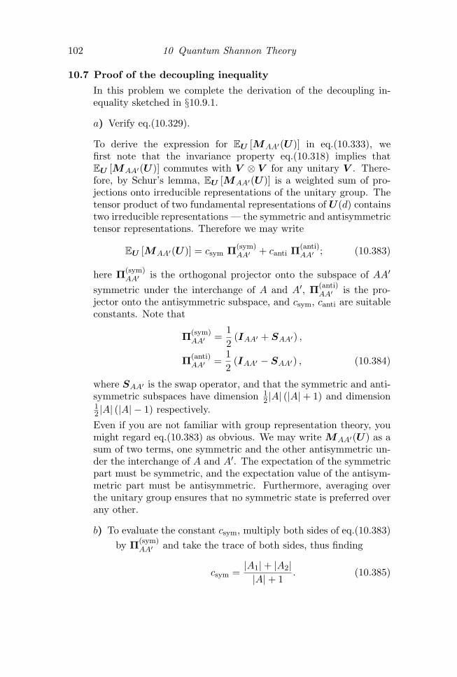
102 10 Quantum Shannon Theory
10.7 Proof of the decoupling inequality
In this problem we complete the derivation of the decoupling in-equality sketched in §10.9.1.
a) Verify eq.(10.329).
To derive the expression for EU [MAA′(U)] in eq.(10.333), wefirst note that the invariance property eq.(10.318) implies thatEU [MAA′(U)] commutes with V ⊗ V for any unitary V . There-fore, by Schur’s lemma, EU [MAA′(U)] is a weighted sum of pro-jections onto irreducible representations of the unitary group. Thetensor product of two fundamental representations of U(d) containstwo irreducible representations — the symmetric and antisymmetrictensor representations. Therefore we may write
EU [MAA′(U)] = csym Π(sym)AA′ + canti Π(anti)
AA′ ; (10.383)
here Π(sym)AA′ is the orthogonal projector onto the subspace of AA′
symmetric under the interchange of A and A′, Π(anti)AA′ is the pro-
jector onto the antisymmetric subspace, and csym, canti are suitableconstants. Note that
Π(sym)AA′ =
12
(IAA′ + SAA′) ,
Π(anti)AA′ =
12
(IAA′ − SAA′) , (10.384)
where SAA′ is the swap operator, and that the symmetric and anti-symmetric subspaces have dimension 1
2 |A| (|A|+ 1) and dimension12 |A| (|A| − 1) respectively.
Even if you are not familiar with group representation theory, youmight regard eq.(10.383) as obvious. We may write MAA′(U) as asum of two terms, one symmetric and the other antisymmetric un-der the interchange of A and A′. The expectation of the symmetricpart must be symmetric, and the expectation value of the antisym-metric part must be antisymmetric. Furthermore, averaging overthe unitary group ensures that no symmetric state is preferred overany other.
b) To evaluate the constant csym, multiply both sides of eq.(10.383)by Π(sym)
AA′ and take the trace of both sides, thus finding
csym =|A1|+ |A2||A|+ 1
. (10.385)

10.12 Exercises 103
c) To evaluate the constant canti, multiply both sides of eq.(10.383))by Π(anti)
AA′ and take the trace of both sides, thus finding
canti =|A1| − |A2||A| − 1
. (10.386)
d) Using
cI =12
(csym + canti) , cS =12
(csym − canti) (10.387)
prove eq.(10.334).
10.8 Fano’s inequality
Suppose X = x, p(x) is a probability distribution for a letter xdrawn from an alphabet of d possible letters, and that XY is thejoint distribution for x and another random variable y which iscorrelated with x. Upon receiving y we estimate the value of x byevaluating a function x(y). We may anticipate that if our estimateis usually correct, then the conditional entropy H(X|Y ) must besmall. In this problem we will confirm that expectation.
Let e ∈ 0, 1 denote a binary random variable which takes the valuee = 0 if x = x(y) and takes the value e = 1 if x 6= x(y), and letXY E denote the joint distribution for x, y, e. The error probabilityPe is the probability that e = 1, averaged over this distribution.Our goal is to derive an upper bound on H(X|Y ) depending on Pe.
a) Show that
H(X|Y ) = H(X|Y E) +H(E|Y )−H(E|XY ). (10.388)
Note that H(E|XY ) = 0 because e is determined when x and yare know, and that H(E|Y ) ≤ H(E) because mutual information isnonnegative. Therefore,
H(X|Y ) ≤ H(X|Y E) +H(E). (10.389)
b) Noting that
H(X|Y E) = p(e = 0)H(X|Y, e = 0) + p(e = 1)H(X|Y, e = 1),(10.390)
and that H(X|Y, e = 0) = 0 (because x = x(y) is determinedby y when there is no error), show that
H(X|Y E) ≤ Pe log2(d− 1). (10.391)

104 10 Quantum Shannon Theory
c) Finally, show that
H(X|Y ) ≤ H2(Pe) + Pe log2(d− 1), (10.392)
which is Fano’s inequality.
d) Use Fano’s inequality to derive eq.(10.50), hence completing theproof that the classical channel capacity C is an upper boundon achievable rates for communication over a noisy channelwith negligible error probability.
10.9 A quantum version of Fano’s inequality
a) In a d-dimensional system, suppose a density operator ρ approx-imates the pure state |ψ〉 with fidelity
F = 〈ψ|ρ|ψ〉 = 1− ε. (10.393)
Show that
H(ρ) ≤ H2(ε) + ε log2(d− 1). (10.394)
Hint: Recall that if a complete orthogonal measurement per-formed on the state ρ has distribution of outcomes X, thenH(ρ) ≤ H(X), where H(X) is the Shannon entropy of X.
b) As in §10.7.2, suppose that the noisy channel NA→B acts on thepure state ψRA, and is followed by the decoding map DB→C .Show that
H(R)ρ − Ic(R 〉B)ρ ≤ 2H(RC)σ, (10.395)
where
ρRB = N (ψRA), σRC = D N (ψRA). (10.396)
Therefore, if the decoder’s output (the state of RC) is almostpure, then the coherent information of the channel N comesclose to matching its input entropy. Hint: Use the data pro-cessing inequality Ic(R 〉C)σ ≤ Ic(R 〉B)ρ and the subaddi-tivity of von Neumann entropy. It is convenient to considerthe joint pure state of the reference system, the output, andenvironments of the dilations of N and D.
c) Suppose that the decoding map recovers the channel input withhigh fidelity,
F (D N (ψRA), ψRC) = 1− ε. (10.397)
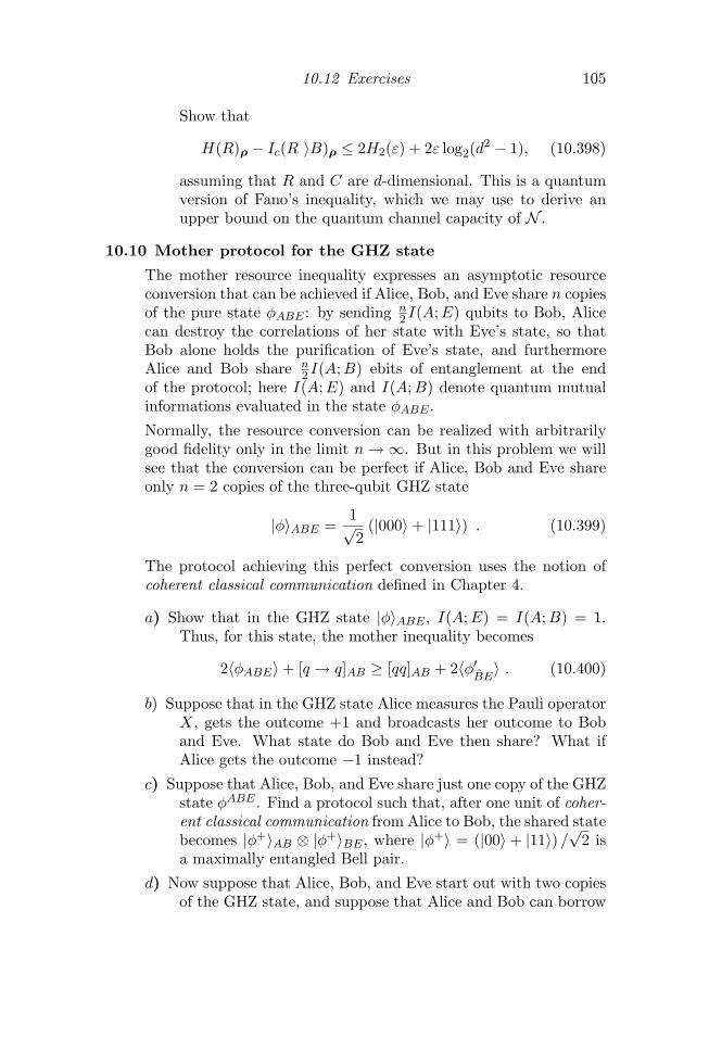
10.12 Exercises 105
Show that
H(R)ρ − Ic(R 〉B)ρ ≤ 2H2(ε) + 2ε log2(d2 − 1), (10.398)
assuming that R and C are d-dimensional. This is a quantumversion of Fano’s inequality, which we may use to derive anupper bound on the quantum channel capacity of N .
10.10 Mother protocol for the GHZ state
The mother resource inequality expresses an asymptotic resourceconversion that can be achieved if Alice, Bob, and Eve share n copiesof the pure state φABE : by sending n
2 I(A;E) qubits to Bob, Alicecan destroy the correlations of her state with Eve’s state, so thatBob alone holds the purification of Eve’s state, and furthermoreAlice and Bob share n
2 I(A;B) ebits of entanglement at the endof the protocol; here I(A;E) and I(A;B) denote quantum mutualinformations evaluated in the state φABE .
Normally, the resource conversion can be realized with arbitrarilygood fidelity only in the limit n→∞. But in this problem we willsee that the conversion can be perfect if Alice, Bob and Eve shareonly n = 2 copies of the three-qubit GHZ state
|φ〉ABE =1√2
(|000〉+ |111〉) . (10.399)
The protocol achieving this perfect conversion uses the notion ofcoherent classical communication defined in Chapter 4.
a) Show that in the GHZ state |φ〉ABE , I(A;E) = I(A;B) = 1.Thus, for this state, the mother inequality becomes
2〈φABE〉+ [q → q]AB ≥ [qq]AB + 2〈φ′BE〉 . (10.400)
b) Suppose that in the GHZ state Alice measures the Pauli operatorX, gets the outcome +1 and broadcasts her outcome to Boband Eve. What state do Bob and Eve then share? What ifAlice gets the outcome −1 instead?
c) Suppose that Alice, Bob, and Eve share just one copy of the GHZstate φABE . Find a protocol such that, after one unit of coher-ent classical communication from Alice to Bob, the shared statebecomes |φ+〉AB ⊗ |φ+〉BE , where |φ+〉 = (|00〉+ |11〉) /
√2 is
a maximally entangled Bell pair.
d) Now suppose that Alice, Bob, and Eve start out with two copiesof the GHZ state, and suppose that Alice and Bob can borrow
106 10 Quantum Shannon Theory
an ebit of entanglement, which will be repaid later, to catalyzethe resource conversion. Use coherent superdense coding toconstruct a protocol that achieves the (catalytic) conversioneq. (10.400) perfectly.
10.11 Degradability of amplitude damping and erasure
The qubit amplitude damping channel NA→Ba.d. (p) discussed in §3.4.3
has the dilation UA→BE such that
U :|0〉A 7→ |0〉B ⊗ |0〉E ,|1〉A 7→
√1− p |1〉B ⊗ |0〉E +
√p |0〉B ⊗ |1〉E ;
a qubit in its “ground state” |0〉A is unaffected by the channel,while a qubit in the “excited state” |1〉A decays to the ground statewith probability p, and the decay process excites the environment.Note that U is invariant under interchange of systems B and Eaccompanied by transformation p ↔ (1 − p). Thus the channelcomplementary to NA→B
a.d. (p) is NA→Ea.d. (1− p).
a) Show that NA→Ba.d. (p) is degradable for p ≤ 1/2. Therefore, the
quantum capacity of the amplitude damping channel is its op-timized one-shot coherent information. Hint: It suffices toshow that
NA→Ea.d. (1− p) = NB→E
a.d. (q) NA→Ba.d. (p), (10.401)
where 0 ≤ q ≤ 1.
The erasure channel NA→Berase (p) has the dilation UA→BE such that
U : |ψ〉A 7→√
1− p |ψ〉B ⊗ |e〉E +√p |e〉B ⊗ |ψ〉E ; (10.402)
Alice’s system passes either to Bob (with probability 1 − p) or toEve (with probability p), while the other party receives the “erasuresymbol” |e〉, which is orthogonal to Alice’s Hilbert space. Because Uis invariant under interchange of systems B and E accompanied bytransformation p↔ (1−p), the channel complementary toNA→B
erase (p)is NA→E
erase (1− p).
b) Show that NA→Berase (p) is degradable for p ≤ 1/2. Therefore, the
quantum capacity of the amplitude damping channel is its op-timized one-shot coherent information. Hint: It suffices toshow that
NA→Eerase (1− p) = NB→E
erase (q) NA→Berase (p), (10.403)
where 0 ≤ q ≤ 1.

10.12 Exercises 107
c) Show that for p ≤ 1/2 the quantum capacity of the erasurechannel is
Q(NA→Berase (p)) = (1− 2p) log2 d, (10.404)
where A is d-dimensional, and that the capacity vanishes for1/2 ≤ p ≤ 1.
10.12 Capacities of the depolarizing channel
Consider the depolarizing channel Ndepol.(p), which acts on a purestate |ψ〉 of a single qubit according to
Ndepol.(p) : |ψ〉〈ψ| 7→(
1− 43p
)|ψ〉〈ψ|+ 4
3p · 1
2I. (10.405)
For this channel, compute the product-state classical capacity C1(p),the entanglement-assisted classical capacity CE(p), and the one-shotquantum capacity Q1(p). Plot the results as a function of p. Forwhat value of p does Q1 hit zero?
The depolarizing channel is not degradable, and in fact the quantumcapacity Q(p) is larger than Q1(p) when the channel is sufficientlynoisy. The function Q(p) is still unknown.
10.13 Noisy superdense coding and teleportation.
a) By converting the entanglement achieved by the mother proto-col into classical communication, prove the noisy superdensecoding resource inequality:
Noisy SD : 〈φABE〉+H(A)[q → q] ≥ I(A;B)[c→ c].(10.406)
Verify that this matches the standard noiseless superdense cod-ing resource inequality when φ is a maximally entangled stateof AB.
b) By converting the entanglement achieved by the mother protocolinto quantum communication, prove the noisy teleportationresource inequality:
Noisy TP : 〈φABE〉+ I(A;B)[c→ c] ≥ Ic(A〉B)[q → q].(10.407)
Verify that this matches the standard noiseless teleportationresource inequality when φ is a maximally entangled state ofAB.

108 10 Quantum Shannon Theory
10.14 The cost of erasure
Erasure of a bit is a process in which the state of the bit is reset to 0.Erasure is irreversible — knowing only the final state 0 after erasure,we cannot determine whether the initial state before erasure was 0or 1. This irreversibility implies that erasure incurs an unavoidablethermodynamic cost. According to Landauer’s Principle, erasing abit at temperature T requires work W ≥ kT log 2. In this problemyou will verify that a particular procedure for achieving erasureadheres to Landauer’s Principle.
Suppose that the two states of the bit both have zero energy. Weerase the bit in two steps. In the first step, we bring the bit intocontact with a reservoir at temperature T > 0, and wait for the bitto come to thermal equilibrium with the reservoir. In this step thebit “forgets” its initial value, but the bit is not yet erased becauseit has not been reset.
We reset the bit in the second step, by slowly turning on a controlfield λ which splits the degeneracy of the two states. For λ ≥ 0, thestate 0 has energy E0 = 0 and the state 1 has energy E1 = λ. Afterthe bit thermalizes in step one, the value of λ increases graduallyfrom the initial value λ = 0 to the final value λ = ∞; the increasein λ is slow enough that the qubit remains in thermal equilibriumwith the reservoir at all times. As λ increases, the probability P (0)that the qubit is in the state 0 approaches unity — i.e., the bit isreset to the state 0, which has zero energy.
(a) For λ 6= 0, find the probability P (0) that the qubit is in thestate 0 and the probability P (1) that the qubit is in the state1.
(b) How much work is required to increase the control field from λto λ+ dλ?
(c) How much work is expended as λ increases slowly from λ = 0to λ = ∞? (You will have to evaluate an integral, which canbe done analytically.)
10.15 The first law of Von Neumann entropy
Writing the density operator in terms of its modular HamiltonianK as in §10.2.6,
ρ =e−K
tr (e−K), (10.408)

10.12 Exercises 109
consider how the entropy S(ρ) = −tr (ρ lnρ) changes when thedensity operator is perturbed slightly:
ρ → ρ′ = ρ + δρ. (10.409)
Since ρ and ρ′ are both normalized density operators, we havetr (δρ) = 0. Show that
S(ρ′)− S(ρ) = tr(ρ′K
)− tr (ρK) +O
((δρ)2
); (10.410)
that is,
δS = δ〈K〉 (10.411)
to first order in the small change in ρ. This statement generalizesthe first law of thermodynamics; for the case of a thermal densityoperator with K = T−1H (where H is the Hamiltonian and T isthe temperature), it becomes the more familiar statement
δE = δ〈H〉 = TδS. (10.412)
10.16 Information gain for a quantum state drawn from the uni-form ensemble
Suppose Alice prepares a quantum state drawn from the ensem-ble ρ(x), p(x) and Bob performs a measurement E(y) yieldingoutcome y with probability p(y|x) = tr (E(y)ρ(x)). As noted in§10.6.1, Bob’s information gain about Alice’s preparation is the mu-tual information I(X;Y ) = H(X) −H(X|Y ). If x is a continuousvariable, while y is discrete, it is more convenient to use the sym-metry of mutual information to write I(X;Y ) = H(Y )−H(Y |X),where
H(Y |X) =∑y
∫dx · p(x) · p(y|x) · log p(y|x); (10.413)
here p(x) is a probability density (that is, p(x)dx is the probabilityfor x to lie in the interval [x, x+ dx]).
For example, suppose that Alice prepares an arbitrary pure state |ϕ〉chosen from the uniform ensemble in a d-dimensional Hilbert space,and Bob performs an orthogonal measurement projecting onto thebasis |ey〉, hoping to learn something about what Alice prepared.Then Bob obtains outcome y with probability
p(y|θ) = |〈ey|ϕ〉|2 ≡ cos2 θ (10.414)

110 10 Quantum Shannon Theory
where θ is the angle between |ϕ〉 and |ey〉. Because Alice’s ensembleis uniform, Bob’s outcomes are also uniformly distributed; henceH(Y ) = log d. Furthermore, the measurement outcome y revealsonly information about θ; Bob learns nothing else about |ϕ〉. There-fore, eq.(10.413) implies that the information gain may be expressedas
I(X;Y ) = log d− d
∫dθ · p(θ) · cos2 θ · log cos2 θ. (10.415)
Here p(θ)dθ is the probability density for the vector |ϕ〉 to point ina direction making angle θ with the axis |ey〉, where 0 ≤ θ ≤ π/2.
a) Show that
p(θ) · dθ = −(d− 1)[1− cos2 θ
]d−2 · d cos2 θ. (10.416)
Hint: Choose a basis in which the fixed axis |ey〉 is
|ey〉 = (1,~0) (10.417)
and write|ϕ〉 = (eiφ cos θ, ψ⊥), (10.418)
where θ ∈ [0, π/2], and |ψ⊥〉 denotes a complex (d−1)-component vector with length sin θ. Now note that the phaseφ resides on a circle of radius cos θ (and hence circumference2π cos θ), while |ψ⊥〉 lies on a sphere of radius sin θ (thus thevolume of the sphere, up to a multiplicative numerical con-stant, is sin2d−3 θ).
b) Now evaluate the integral eq. (10.415) to show that the informa-tion gain from the measurement, in nats, is
I(X;Y ) = ln d−(
12
+13
+ · · ·+ 1d
). (10.419)
(Information is expressed in nats if logarithms are natural log-arithms; I in nats is related to I in bits by Ibits = Inats/ ln 2.)Hint: To evaluate the integral∫ 1
0dx(1− x)px lnx , (10.420)
observe thatx lnx =
d
dsxs∣∣∣s=1
, (10.421)
and then calculate∫ 10 dx(1− x)
pxs by integrating by parts re-peatedly.

10.12 Exercises 111
c) Show that in the limit of large d, the information gain, in bits,approaches
Id=∞ =1− γ
ln 2= .60995 . . . , (10.422)
where γ = .57721 . . . is Euler’s constant.
Our computed value of H(Y |X) may be interpreted in anotherway: Suppose we fix an orthogonal measurement, choose a typi-cal state, and perform the measurement repeatedly on that chosenstate. Then the measurement outcomes will not be uniformly dis-tributed. Instead the entropy of the outcomes will fall short ofmaximal by .60995 bits, in the limit of large Hilbert space dimen-sion.

References
[1] M. M. Wilde, Quantum Information Theory (Cambridge, 2013).
[2] T. M. Cover and J. A. Thomas, Information Theory (Wiley, 1991).
[3] C. E Shannon and W. Weaver, The Mathematical Theory of Communication(Illinois, 1949).
[4] M. A. Nielsen and I. L. Chuang, Quantum Computation and Quantum In-formation (Cambridge, 2000).
[5] A. Wehrl, General properties of entropy, Rev. Mod. Phys. 50, 221 (1978).
[6] E. H. Lieb and M. B. Ruskai, A fundamental property of quantum-mechanical entropy, Phys. Rev. Lett. 30, 434 (1973).
[7] P. Hayden, R. Jozsa, D. Petz, and A. Winter, Structure of states whichsatisfy strong subadditivity with equality, Comm. Math. Phys. 246, 359-374 (2003).
[8] M. A. Nielsen and J. Kempe, Separable states are more disordered globallythan locally, Phys. Rev. Lett. 86, 5184 (2001).
[9] J. Bekenstein, Universal upper bound on the entropy-to-energy ration ofbounded systems, Phys. Rev. D 23, 287 (1981).
[10] H. Casini, Relative entropy and the Bekenstein bound, Class. Quant. Grav.25, 205021 (2008).
[11] P. J. Coles, M. Berta, M. Tomamichel, S. Wehner, Entropic uncertaintyrelations and their applications, arXiv:1511.04857 (2015).
[12] H. Maassen and J. Uffink, Phys. Rev. Lett. 60, 1103 (1988).
[13] B. Schumacher, Quantum coding, Phys. Rev. A 51, 2738 (1995).
[14] R. Jozsa and B. Schumacher, A new proof of the quantum noiseless codingtheory, J. Mod. Optics 41, 2343-2349 (1994).
[15] C. H. Bennett, H. J. Bernstein, S. Popescu, and B. Schumacher, Concen-trating partial entanglement by local operations, Phys. Rev. A 53, 2046(1996).
112

References 113
[16] R. Horodecki, P. Horodecki, M. Horodecki, and K. Horodecki, Quantumentanglement, Rev. Mod. Phys. 81, 865 (2009).
[17] F. G. S. L. Brandao and M. B. Plenio, A reversible theory of entanglementand its relation to the second law, Comm. Math. Phys. 295, 829-851 (2010).
[18] M. Christandl and A. Winter, “Squashed entanglement”: an additive en-tanglement measure, J. Math. Phys. 45, 829 (2004).
[19] M. Koashi and A. Winter, Monogamy of quantum entanglement and othercorrelations, Phys. Rev. A 69, 022309 (2004).
[20] F. G. S. L. Brandao, M. Cristandl, and J. Yard, Faithful squashed entan-glement, Comm. Math. Phys. 306, 805-830 (2011).
[21] A. C. Doherty, P. A. Parrilo, and F. M. Spedalieri, Complete family ofseparability criteria, Phys. Rev. A 69, 022308 (2004).
[22] A. S. Holevo, Bounds for the quantity of information transmitted by aquantum communication channel, Probl. Peredachi Inf. 9, 3-11 (1973).
[23] A. Peres and W. K. Wootters, Optimal detection of quantum information,Phys. Rev. Lett 66, 1119 (1991).
[24] A. S. Holevo, The capacity of the quantum channel with general signalstates, arXiv: quant-ph/9611023.
[25] B. Schumacher and M. D. Westmoreland, Sending classical information vianoisy quantum channels, Phys. Rev. A 56, 131-138 (1997).
[26] M. B. Hastings, Superadditivity of communication capacity using entangledinputs, Nature Physics 5, 255-257 (2009).
[27] M. Horodecki, P. W. Shor, and M. B. Ruskai, Entanglement breaking chan-nels, Rev. Math. Phys. 15, 629-641 (2003).
[28] P. W. Shor, Additivity of the classical capacity for entanglement-breakingquantum channels, J. Math. Phys. 43, 4334 (2002).
[29] B. Schumacher and M. A. Nielsen, Quantum data processing and errorcorrection, Phys. Rev. A 54, 2629 (1996).
[30] B. Schumacher, Sending entanglement through noisy quantum channels,Phys. Rev. A 54, 2614 (1996).
[31] H. Barnum, E. Knill, and M. A. Nielsen, On quantum fidelities and channelcapacities, IEEE Trans. Inf. Theory 46, 1317-1329 (2000).
[32] S. Lloyd, Capacity of the noisy quantum channel, Phys. Rev. A 55, 1613(1997).
[33] P. W. Shor, unpublished (2002).
[34] I. Devetak, The private classical capacity and quantum capacity of a quan-tum channel, IEEE Trans. Inf. Theory 51, 44-55 (2005).
[35] I. Devetak and A. Winter, Distillation of secret key and entanglement fromquantum states, Proc. Roy. Soc. A 461, 207-235 (2005).

114 References
[36] B. Schumacher and M. D. Westmoreland, Approximate quantum error cor-rection, Quant. Inf. Proc. 1, 5-12 (2002).
[37] M. Horodecki, J. Oppenheim, and A. Winter, Quantum state merging andnegative information, Comm. Math. Phys. 269, 107-136 (2007).
[38] P. Hayden, M. Horodecki, A. Winter, and J. Yard, Open Syst. Inf. Dyn. 15,7-19 (2008).
[39] A. Abeyesinge, I. Devetak, P. Hayden, and A. Winter, Proc. Roy. Soc. A,2537-2563 (2009).
[40] E. Lubkin, Entropy of an n-system from its correlation with a k-reservoir,J. Math. Phys. 19, 1028 (1978).
[41] S. Lloyd and H. Pagels, Complexity as thermodynamic depth, Ann. Phys.188, 186-213 (1988)
[42] D. N. Page, Average entropy of a subsystem, Phys. Rev. Lett. 71, 1291(1993).
[43] I. Devetak, A. W. Harrow, and A. Winter, A family of quantum protocols,Phys. Rev. Lett. 93, 230504 (2004).
[44] I. Devetak, A. W. Harrow, and A. Winter, A resource framework for quan-tum Shannon theory, IEEE Trans. Inf. Theory 54, 4587-4618 (2008).
[45] I. Devetak and P. W. Shor, The capacity of a quantum channel for simul-taneous transmission of classical and quantum information, Comm. Math.Phys. 256, 287-303 (2005).
[46] C. H. Bennett, P. W. Shor, J. A. Smolin, and A. V. Thapliyal,Entanglement-assisted classical capacity of noisy quantum channels, Phys.Rev. Lett. 83, 3081 (1999).
[47] C. H. Bennett, P. W. Shor, J. A. Smolin, and A. V. Thapliyal,Entanglement-assisted classical capacity of a quantum channel and the re-verse Shannon theorem, IEEE Trans. Inf. Theory 48, 2637-2655 (2002).
[48] P. W. Shor and J. A. Smolin, Quantum error-correcting codes need notcompletely reveal the error syndrome, arXiv:quant-ph/9604006.
[49] D. P. DiVincenzo, P. W. Shor, and J. A. Smolin, Quantum channel capacityof very noisy channels, Phys. Rev. A 57, 830 (1998).
[50] G. Smith and J. Yard, Quantum communication with zero-capacity chan-nels, Science 321, 1812-1815 (2008).
[51] L. del Rio, J. Aberg, R. Renner, O. Dahlsten, and V. Vedral, The thermo-dynamic meaning of negative entropy, Nature 474, 61-63 (2011).
[52] P. Hayden and J. Preskill, Black holes as mirrors: quantum information inrandom subsystems, JHEP 09, 120 (2007).
[53] Y. Sekino and L. Susskind, Fast scramblers, JHEP 10, 065 (2008).


![Quantum Information - Primitive notions and quantum ...johnboccio.com/research/quantum/notes/09104222.pdf · Quantum Information - Primitive notions and quantum correlations ... Bellac[LeBellac2006].](https://static.fdocuments.net/doc/165x107/5b68b4bc7f8b9a68538ce530/quantum-information-primitive-notions-and-quantum-quantum-information.jpg)