
Quantum Geometry and Quantum Field Theoryrobert/docs/phd_thesis.pdfQuantum Geometry and Quantum...
138
Quantum Geometry and Quantum Field Theory Robert Oeckl Downing College Cambridge September 2000 A dissertation submitted for the degree of Doctor of Philosophy at the University of Cambridge
Transcript of Quantum Geometry and Quantum Field Theoryrobert/docs/phd_thesis.pdfQuantum Geometry and Quantum...

Quantum Geometry and
Quantum Field Theory
Robert Oeckl
Downing College
Cambridge
September 2000
A dissertation submitted for
the degree of Doctor of Philosophy
at the University of Cambridge

Preface
This dissertation is based on research done at the Department of Applied Mathematics and
Theoretical Physics, University of Cambridge, in the period from October 1997 to August
2000. It is original except where reference is made to the work of others. Chapter 4 in its
entirety and Chapter 2 partly (as specified therein) represent work done in collaboration with
Shahn Majid. All other chapters represent solely my own work. No part of this dissertation
nor anything substantially the same has been submitted for any qualification at any other
university. Most of the material presented has been published or submitted for publication
in the following papers:
• [Oec99b] R. Oeckl, Classification of differential calculi on Uq(b+), classical limits, and
duality, J. Math. Phys. 40 (1999), 3588–3603.
• [MO99] S. Majid and R. Oeckl, Twisting of Quantum Differentials and the Planck Scale
Hopf Algebra, Commun. Math. Phys. 205 (1999), 617–655.
• [Oec99a] R. Oeckl, Braided Quantum Field Theory, Preprint DAMTP-1999-82, hep-
th/9906225.
• [Oec00b] R. Oeckl, Untwisting noncommutative Rd and the equivalence of quantum field
theories, Nucl. Phys. B 581 (2000), 559–574.
• [Oec00a] R. Oeckl, The Quantum Geometry of Spin and Statistics, Preprint DAMTP-
2000-81, hep-th/0008072.
ii

Acknowledgements
First of all, I would like to thank my supervisor Shahn Majid. Besides helping and encouraging
me in my studies, he managed to inspire me with a deep fascination for the subject. Many
other people in the department have contributed to making this an enjoyable time for me. In
particular, I would like to mention my fellow students Marco Barozzo, Kumaran Damodaran,
Tathagata Dasgupta, Steffen Krusch, Hendryk Pfeiffer, Andrew Tolley, and Fabian Wagner.
I am grateful to the German Academic Exchange Service (DAAD) and the Engineering and
Physical Sciences Research Council (EPSRC) for the funding of much of this work.
Finally, my thanks go to my parents, my sister, and my brother, as well as my friends in
Cambridge and elsewhere, for their support and care.
iii

Contents
Introduction 1
1 Basics 6
1.1 Hopf algebras . . . . . . . . . . . . . . . . . . . . . . . . . . . . . . . . . . . . 6
1.1.1 Quantum Groups . . . . . . . . . . . . . . . . . . . . . . . . . . . . . . 7
1.2 Representation Theory . . . . . . . . . . . . . . . . . . . . . . . . . . . . . . . 8
1.2.1 (Braided) Monoidal Categories . . . . . . . . . . . . . . . . . . . . . . 8
1.2.2 Hopf Algebra Module Categories . . . . . . . . . . . . . . . . . . . . . 11
1.3 Quantum Differentials . . . . . . . . . . . . . . . . . . . . . . . . . . . . . . . 15
1.3.1 First Order Differential Calculi . . . . . . . . . . . . . . . . . . . . . . 15
1.3.2 Exterior Differential Algebras . . . . . . . . . . . . . . . . . . . . . . . 17
2 Twisting Theory 20
2.1 Hopf Algebras . . . . . . . . . . . . . . . . . . . . . . . . . . . . . . . . . . . . 21
2.2 Module Categories . . . . . . . . . . . . . . . . . . . . . . . . . . . . . . . . . 22
2.3 Deformation Quantisation . . . . . . . . . . . . . . . . . . . . . . . . . . . . . 28
2.4 Quantum Differentials . . . . . . . . . . . . . . . . . . . . . . . . . . . . . . . 29
2.4.1 Covariant Differentials . . . . . . . . . . . . . . . . . . . . . . . . . . . 29
2.4.2 Bicovariant Differentials over Quantum Groups . . . . . . . . . . . . . 30
3 Differential Calculi on Uq(b+) 32
3.1 Uq(b+) and its Classical Limits . . . . . . . . . . . . . . . . . . . . . . . . . . 34
3.2 Classification on Cq(B+) and Uq(b+) . . . . . . . . . . . . . . . . . . . . . . . 35
3.3 Classification in the Classical Limit . . . . . . . . . . . . . . . . . . . . . . . . 41
3.4 The Dual Classical Limit . . . . . . . . . . . . . . . . . . . . . . . . . . . . . 44
3.5 Remarks on κ-Minkowski Space and Integration . . . . . . . . . . . . . . . . . 48
3.A Appendix: The Adjoint Coaction on Uq(b+) . . . . . . . . . . . . . . . . . . . 50
iv

4 Quantum Geometry of the Planck Scale Hopf Algebra 52
4.1 The Cocycle Twist . . . . . . . . . . . . . . . . . . . . . . . . . . . . . . . . . 53
4.2 Differential Calculi . . . . . . . . . . . . . . . . . . . . . . . . . . . . . . . . . 55
4.3 Quantum Poisson Bracket . . . . . . . . . . . . . . . . . . . . . . . . . . . . . 60
4.4 Fourier Theory . . . . . . . . . . . . . . . . . . . . . . . . . . . . . . . . . . . 63
5 Spin and Statistics 69
5.1 Spin . . . . . . . . . . . . . . . . . . . . . . . . . . . . . . . . . . . . . . . . . 70
5.2 Statistics . . . . . . . . . . . . . . . . . . . . . . . . . . . . . . . . . . . . . . 71
5.3 Braided Categories and Statistics . . . . . . . . . . . . . . . . . . . . . . . . . 73
5.4 Quantum Groups and Statistics . . . . . . . . . . . . . . . . . . . . . . . . . . 74
5.5 Unifying Spin and Statistics . . . . . . . . . . . . . . . . . . . . . . . . . . . . 76
6 Braided Quantum Field Theory – Foundations 79
6.1 The Braided Path Integral . . . . . . . . . . . . . . . . . . . . . . . . . . . . . 80
6.1.1 Gaussian Integration . . . . . . . . . . . . . . . . . . . . . . . . . . . . 80
6.1.2 Path Integration . . . . . . . . . . . . . . . . . . . . . . . . . . . . . . 83
6.1.3 Special Cases: Bosons and Fermions . . . . . . . . . . . . . . . . . . . 85
6.2 Braided Feynman Diagrams . . . . . . . . . . . . . . . . . . . . . . . . . . . . 87
6.2.1 Perturbation Theory . . . . . . . . . . . . . . . . . . . . . . . . . . . . 88
6.2.2 The Diagrams . . . . . . . . . . . . . . . . . . . . . . . . . . . . . . . . 89
6.2.3 Bosonic and Fermionic Feynman Rules . . . . . . . . . . . . . . . . . . 91
7 Braided Quantum Field Theory – Special Cases 94
7.1 Anyonic Statistics and Quons . . . . . . . . . . . . . . . . . . . . . . . . . . . 95
7.2 Symmetric Braided Quantum Field Theory . . . . . . . . . . . . . . . . . . . 97
7.3 Braided QFT on Quantum Homogeneous Spaces . . . . . . . . . . . . . . . . 98
7.3.1 Quantum Homogeneous Spaces . . . . . . . . . . . . . . . . . . . . . . 99
7.3.2 Diagrammatic Techniques . . . . . . . . . . . . . . . . . . . . . . . . . 100
7.4 Braided QFT on Compact Quantum Spaces . . . . . . . . . . . . . . . . . . . 102
7.4.1 Braided Spaces of Infinite Dimension . . . . . . . . . . . . . . . . . . . 102
7.4.2 Cosemisimplicity and Peter-Weyl Decomposition . . . . . . . . . . . . 103
8 Quantum Field Theory on Noncommutative Rd 104
8.1 Noncommutative Rd as a Twist . . . . . . . . . . . . . . . . . . . . . . . . . . 106
8.1.1 A Remark on the Noncommutative Torus . . . . . . . . . . . . . . . . 108
8.2 Towards Quantum Field Theory . . . . . . . . . . . . . . . . . . . . . . . . . 109
v

8.3 Equivalences for Quantum Field Theory . . . . . . . . . . . . . . . . . . . . . 110
8.4 Perturbative Consequences . . . . . . . . . . . . . . . . . . . . . . . . . . . . 112
8.5 Additional Symmetries . . . . . . . . . . . . . . . . . . . . . . . . . . . . . . . 114
8.5.1 Space-Time Symmetry . . . . . . . . . . . . . . . . . . . . . . . . . . . 114
8.5.2 Gauge Symmetry . . . . . . . . . . . . . . . . . . . . . . . . . . . . . . 115
8.A Appendix . . . . . . . . . . . . . . . . . . . . . . . . . . . . . . . . . . . . . . 115
9 φ4-Theory on the Quantum 2-Sphere 117
9.1 The Decomposition of SUq(2) and S2q . . . . . . . . . . . . . . . . . . . . . . 118
9.2 The Free Propagator . . . . . . . . . . . . . . . . . . . . . . . . . . . . . . . . 120
9.3 Interactions . . . . . . . . . . . . . . . . . . . . . . . . . . . . . . . . . . . . . 121
9.4 Renormalisation . . . . . . . . . . . . . . . . . . . . . . . . . . . . . . . . . . 123
9.A Appendix: Coquasitriangular Structure of SUq(2) . . . . . . . . . . . . . . . . 124
Bibliography 126
vi

Introduction
Reading the title of this dissertation one might ask: What is quantum geometry? or What
does it have to do with quantum field theory? The first of these questions we will try to
answer immediately. For the second we hope that the following chapters hold at least a
partial answer.
More familiar perhaps than the term quantum geometry are the terms that it is meant to
subsume: noncommutative geometry and quantum groups. Although both belong to the realm
of mathematics, their evolution has been very much connected with developments in physics,
particularly quantum physics. The story begins with the early days of quantum mechanics.
Heisenberg’s commutation relations
[X,P ] = i~
imply that the geometry of classical phase space is lost. If coordinates (such as X and P )
on a phase space cease to commute then there can be no such space. Instead, one viewed X
and P purely as operators on a Hilbert space. Functional analysis succeeded geometry. It
has been dominating quantum mechanics ever since. In spite of this, the idea, in one form or
other, that this operator algebra forms some kind of “noncommutative geometric space” has
accompanied quantum mechanics almost from the beginning. However, for a long time, no
serious attempt has been made to develop such a generalised geometry.
Algebraic geometry is built on a correspondence between “spaces” and commutative alge-
bras. The correspondence associates with a space the algebra of functions on it. Geometric
notions are then expressed in a purely algebraic language. This principle turns out to be
the right starting point for a generalised geometry. While for algebraic geometry the spaces
are affine schemes, a correspondence that is closer to differential geometry is given by the
Gelfand-Naimark theorem. In this case the spaces are topological spaces and the algebras
commutative C∗-algebras.
Around 1980, an approach was initiated by Alain Connes which has become widely known
as noncommutative geometry [Con80, Con85, Con94]. This approach is very much in the func-
tional analytic tradition of quantum mechanics. It introduces notions of Dirac operator, dif-
1

2 Introduction
ferential structures, metric structures, vector bundles, etc. in a context of (noncommutative)
operator algebras leading to many interesting developments in mathematics.
A quite different development originated also around 1980. It came out of the study
of quantum integrable systems by the (then) Leningrad school of Ludwig D. Faddeev and
others. They encountered generalised symmetries that were not described by groups but
could be related to groups. From these emerged the q-deformations of Lie algebras and Lie
groups [Jim85, Dri85, Wor87, RTF90]. It was then also realised by Vladimir G. Drinfeld that
they are examples of a more general structure, called a quantum group. He developed the
mathematical theory of quantum groups extensively in the 1980’s [Dri87]. The underlying
structure is that of a Hopf algebra, a concept that had appeared already much earlier in the
context of group cohomology.
To connect the two developments we note that the correspondence between “spaces” and
commutative algebras extends to (algebraic) groups. The extra structure provided by the
group multiplication corresponds on the algebra side to the additional structure that makes
a commutative algebra a commutative Hopf algebra. Thus, (noncommutative) Hopf algebras
are generalisations of groups in the same way as (noncommutative) algebras are generalisations
of spaces. The (algebraic) theory that encompasses both is called quantum geometry.1
Interesting mathematical developments have taken place since the early days. The rep-
resentation theory of quantum groups is very rich and leads to braided monoidal categories
[JS86]. This in turn has led to new insights into knot theory and invariants of 3-manifolds.
Many examples of quantum spaces have been investigated since the late 80’s including defor-
mations of Rn, of spheres, of projective spaces, etc. Differential structures on quantum groups
were introduced [Wor89] as well as quantum principal bundles and connections [BM93].
Besides the purely mathematical attraction of quantum geometry there are very good
reasons to expect it to play an important role in physics. This goes far beyond the initial
application of quantum groups as symmetries of certain quantum integrable systems. One
particularly intriguing idea is that quantum geometry might lend a far better description
of space-time at the Planck scale than ordinary differential geometry does. Based on the
persistent inability to unite gravity with quantum field theory it has long been conjectured
that space-time at short distances might have a discrete or foam-like structure. It seems that,
with the emergence of quantum geometry, for the first time the tools for such a description
are at hand.
As early as the 1940’s it was proposed that space-time coordinates might be noncommuting
1It is worth mentioning that the term quantum geometry has appeared in recent years also in other contexts,
notably in loop quantum gravity and string theory. This is not necessarily related to the meaning we attach
to it here.

3
observables [Sny47]. This was then motivated by the hope that the infinities arising at very
short distances in quantum field theory might be regularised in this way. It took several
decades – until the emergence of quantum groups and noncommutative geometry – for further
development of such ideas to occur. Shortly after their introduction, Shahn Majid suggested
a role for quantum groups in Planck scale physics as a unified description of the observable
algebra and the gravitational curvature [Maj88]. (See Chapter 4 for further developments
of this idea.) Around 1990 Alain Connes and collaborators initiated a reformulation of the
standard model using noncommutative geometry to describe its internal degrees of freedom
[CL90, Con94]. At about the same time quantum deformations of Minkowski space and its
symmetries were introduced [PW90, CSSW90, OSWZ92] with the motivation to obtain new
physical models by deformation. Braided categories were found to describe generalised particle
statistics in the context of algebraic quantum field theory [FRS89, FG90], indicating quantum
group symmetries (see Chapter 5). The interest in noncommutative geometry was boosted
in 1997 with the emergence of noncommutative spaces in string theory [CDS98, SW99]. (See
Chapter 8 for a development on this.) Quantum groups have also appeared in the loop
approach at quantum gravity [MS96]. Both indicate an important role for quantum geometry
in fundamental physics. The idea of noncommutativity as a regulator has found a successful
application in “fuzzy physics”, where function algebras are approximated by finite dimensional
algebras [Mad92, Mad95, GKP96]. This is similar to a lattice approximation, but without
the breaking of space-time symmetries. In contrast, the more ambitious aim of a continuous
regularisation of quantum field theory by quantum deformation of symmetries (as proposed
in [Maj90b]) has been open for some time. It has found its first realisation only recently in
the work presented here (see Chapter 9).
This dissertation aims at contributing to some of the mentioned developments as well as
introducing new approaches. Its most central development is braided quantum field theory,
a generalisation of quantum field theory to braided spaces (Chapter 6). This allows the
construction of quantum field theories with quantum group symmetries and with general braid
statistics. It forms the basis for much of the other material (Chapters 7–9) or is connected to it
(Chapter 5). At this point we would like to emphasise that our approach departs considerably
from the functional analytic tradition of quantum mechanics (as it seems any framework must
do that allows for radical generalisations of the space-time concept). In particular, our path
integral no longer corresponds in general to a canonical description with field operators on
a Hilbert space. Whether this is a weakness or a strength remains to be seen. The anyonic
example of Chapter 7 appears to point towards the latter.

4 Introduction
Overview
Chapter 1 serves as a review for material that underlies much of this dissertation. In partic-
ular, some facts about the representation theory of Hopf algebras are recalled which are used
in most of the following chapters. Furthermore, aspects of quantum differential calculi are
reviewed which are used in Chapters 2–4.
Chapter 2 presents an extension of Drinfeld’s twisting theory: A twist relating two Hopf
algebras gives rise to an equivalence between the module categories of the two Hopf algebras.
We show that such an equivalence holds for many other representation categories as well.
Furthermore this gives rise to a 1-1 correspondence between differential calculi on quantum
spaces related by twist.
Differential calculi on the quantum group Uq(b+) are investigated in Chapter 3. We give
a complete classification and detailed examination of the classical limit q → 1 and its dual.
At the end we comment on the relation to κ-Minkowski space.
The quantum differential geometry of the Planck scale Hopf algebra [Maj88] is investigated
in Chapter 4. This is a toy model for physics at the Planck scale. The differential calculi and
exterior algebra on it are constructed using results from both previous chapters. The quantum
geometry gives rise to a quantum Poisson bracket, suggesting a deviation from standard
quantum mechanics at strong curvature. A Fourier transform is developed implementing a
T-duality-like self-duality of the model.
Chapter 5 examines the quantum group symmetries behind spin and statistics. We show
that these symmetries can be unified in the presence of a spin-statistics theorem. The Bose-
Fermi case as well as the more general anyonic case are considered.
Braided quantum field theory is introduced in Chapter 6. It employs a path integral
formalism based on Gaussian integration in braided categories which we review. We obtain
a generalisation of Wick’s theorem. Based on this we develop perturbation theory leading
to braided Feynman diagrams, which generalise ordinary Feynman diagrams. Bosonic and
Fermionic path integrals and Feynman rules are recovered as special cases.
The remaining chapters concern applications of braided quantum field theory. In Chap-
ter 7 special cases are considered. First, the quons studied by Greenberg [Gre91] are in-
vestigated as an example of anyonic statistics. We show that braided quantum field theory
provides the path integral counterpart to the usual canonical approach to quons. Then, we
show that for symmetric braiding a correspondence between braided and ordinary Feynman
diagrams can be established. In particular, this applies to Bosons and Fermions. Finally,
methods are developed for quantum field theory on quantum homogeneous spaces and on
compact quantum spaces.

5
In Chapter 8, quantum field theory on the noncommutative Rd arising in a certain limit
of string theory is investigated. We show how this space is related to ordinary Rd by a
Drinfeld twist. Using the twisting theory in conjunction with braided quantum field theory
leads to an equivalence relating quantum field theories on ordinary and noncommutative
Rd. The equivalence exchanges commutativity with noncommutativity and ordinary with a
momentum-dependent statistics.
We construct φ4-theory on the quantum 2-sphere in Chapter 9 using the results about
homogeneous and compact quantum spaces of Chapter 7. The free propagator is obtained
as well as the tadpole diagram. The latter is responsible for making the ordinary φ4-theory
divergent. We show that the divergence is regularised in the noncommutative regime q > 1.
The formalism suggests that divergences of any degree could be regularised in this way. A
diagrammatic interpretation of renormalisation of φ4-theory is obtained.

Chapter 1
Basics
In this chapter we review some basic concepts of quantum group theory that underly much
of this work.
Section 1.1 recalls definitions of Hopf algebra and (co)quasitriangular structures. This is
followed by a brief explanation of our use of the term quantum group. Section 1.2 discusses
general aspects of the representation theory of Hopf algebras. Some of this is relevant to all of
the following chapters. Section 1.3 introduces the notion of differential calculus and exterior
algebra for quantum groups which is needed for Chapters 2, 3, and 4.
To fix our notation, we use the symbols ∆, ε, and S respectively to denote the coproduct,
counit, and antipode of a Hopf algebra, see Section 1.1. For the coproduct we frequently
employ Sweedler’s component notation ∆h = h(1) ⊗ h(2) etc., with summation implied. We
adopt a similar notation v 7→ v(1) ⊗ v(2) and v 7→ v(1) ⊗ v(2) for left and right coactions, see
Section 1.2.2. A braiding will generally be denoted by ψ, see Section 1.2.1. In this chapter as
well as Chapter 2 certain tensor products are denoted by . In the other chapters only the
symbol ⊗ is used. We write a circle for the composition of maps. k denotes a general field.
Standard references on Hopf algebras are the books by Sweedler [Swe69] and Abe [Abe80].
For modern accounts of quantum group theory see, e.g., the text-books by Majid [Maj95b],
Chari and Pressley [CP94], and Klimyk and Schmudgen [KS97].
1.1 Hopf algebras
We recall the definitions of a Hopf algebra and those of (co)quasitriangular structures to be
found in any text-book on quantum groups.
Recall that an associative algebra A is a vector space together with a map · : A⊗A→ A
so that · (· ⊗ id) = · (id⊗·) as maps A ⊗ A ⊗ A → A. A unit is an element 1 ∈ A
so that 1 · a = a · 1 = a for all a ∈ A. Equivalently, a unit is a map η : k → A so that
6

1.1 Hopf algebras 7
· (id⊗ η) = · (η⊗ id) = id as maps A→ A.
Dually, a coassociative coalgebra C is a vector space together with a map ∆ : C → C ⊗Cso that (∆⊗ id) ∆ = (id⊗∆) ∆ as maps C → C ⊗ C ⊗ C. A counit is a map ε : C → kso that (ε⊗ id) ∆ = (id⊗ ε) ∆ as maps C → C. We also use Sweedler’s notation for
coproducts ∆ c = c(1) ⊗ c(2), with summation implied. Due to coassociativity, this notation
can be extended to multiple applications of the coproduct in the obvious way.
A bialgebra B is both an associative algebra with a unit and a coassociative coalgebra
with a counit. Furthermore, the two structures are required to be compatible in the obvious
way, i.e. ∆(ab) = a(1)b(1) ⊗ a(2)b(2) and ε(ab) = ε(a) ε(a) and ∆ 1 = 1⊗ 1 for all a, b ∈ B.
A Hopf algebra H is a bialgebra with a map S : H → H with the property (Sh(1))h(2) =
h(1) Sh(2) = ε(h)1 for all h ∈ H. S is called the antipode.
Definition 1.1.1. A quasitriangular structure (also known as “universal R-matrix”) on a
Hopf algebra H is an invertible element R ∈ H ⊗H so that
(∆⊗ id)R = R13R23, (id⊗∆)R = R13R12, τ ∆h = R(∆h)R−1 ∀h ∈ H,
where R with indices denotes the obvious extension to H ⊗H ⊗H supplemented by the unit
and τ denotes the map that exchanges tensor factors.
Definition 1.1.2. A coquasitriangular structure on a Hopf algebra H is a convolution-
invertible map R : H ⊗H → k so that
R(ab⊗ c) = R(a⊗ c(1))R(b⊗ c(2)), R(a⊗ bc) = R(a(1) ⊗ c)R(a(2) ⊗ b),b(1)a(1)R(a(2) ⊗ b(2)) = R(a(1) ⊗ b(1))a(2)b(2)
for all a, b, c ∈ H.
1.1.1 Quantum Groups
We comment here on our use of the term quantum group in this work.
Commutative Hopf algebras provide an equivalent description of group structures as in
the following well-known example.
Example 1.1.3. Let G be a compact Lie group. Denote the set of algebraic functions1 on G
by C(G). Then C(G) forms a commutative Hopf algebra as follows:
1(g) = 1, (f · h)(g) = f(g)h(g),
ε f = f(e), ∆ f(g, g′) = f(gg′), (S f)(g) = f(g−1),
1These are the functions that are obtained as matrix elements of finite dimensional representations.

8 Basics
where f, h ∈ C(G) while g, g′ ∈ G and e denotes the unit element in G. For the coproduct
observe the implicit isomorphism C(G)⊗C(G) ∼= C(G×G) which holds due to the Peter-Weyl
theorem.
This example represents very much the point of view we take on how the concept of a (not
necessarily commutative) Hopf algebra generalises the concept of a group. We use the term
quantum group with this setting in mind: A Hopf algebra as a generalised function algebra
on a group. Consequently, we are usually interested in coactions rather than actions (see
Section 1.2.2) and coquasitriangular rather than quasitriangular structures.
Due to the self-duality of the axioms of a Hopf algebra there is also the dual point of view,
where the Hopf algebra plays the role of the enveloping algebra of a Lie algebra or that of a
group algebra. We occasionally employ this point of view as well, in particular in Chapters 3
and 4. An advantage of the “function algebra” over the “enveloping algebra” setting lies in
the fact that the global structure of the “group” is not lost. This plays an essential role in
Chapter 5.
Note that some authors use the term quantum group in a narrower sense, so as to only
denote q-deformations of Lie groups and enveloping algebras.
1.2 Representation Theory
1.2.1 (Braided) Monoidal Categories
Intuitively speaking, a monoidal category is a category with a tensor product. In particular,
the category of vector spaces is a monoidal category in this way. The formal definition is as
follows:
Definition 1.2.1. A monoidal category is a category C together with a functor : C×C → Cand a unit object 1 ∈ C satisfying the following conditions:
(i) There is a natural equivalence ΦU,V,W : U (V W )→ (U V )W satisfying
(U V ) (W X)
Φ
U (V (W X))
Φ
idΦ
((U V )W )X
U ((V W )X)Φ
(U (V W ))XΦid

1.2 Representation Theory 9
(ii) There are natural equivalences ρU : U 1→ U and λU : 1 U → U satisfying
U (1 V )Φ
idλ
(U 1) V
ρid
U V
Definition 1.2.2. A functor F : C → D between monoidal categories is a monoidal functor if
F(1C) = 1D and there is a natural equivalence cU,V : F(U)D F(V )→ F(U C V ) satisfying
the “associativity condition” (i)
F(U C V )D F(W )
c
(F(U)D F(V ))D F(W )
ΦC
cD id
F((U C V )C W )
F(ΦC)
F(U)D (F(V )D F(W ))
idDc
F(U C (V C W ))
F(U)D F(V C W )
c
and the “unit conditions” (ii)
F(1C)D F(U)c
id
F(1C C U)
F(λC)
1D D F(U)λD
F(U)
F(U)D F(1C)c
id
F(U C 1C)
F(ρC)
F(U)D 1D ρDF(U)
A monoidal category is called strict if all the natural equivalences Φ, ρ, and λ are identities.
This is the only case of interest to us in the following. In particular, it applies to the category
of vector spaces with the ordinary tensor product ⊗.
An additional important structure for monoidal categories is a braiding. This is an invert-
ible functor ψV,W : V W →W V for objects V , W obeying an associativity condition. A
monoidal category equipped with such a braiding is also called a braided monoidal category
(or “quasitensor category”). The definitions are as follows.
Definition 1.2.3. A braided monoidal category is a monoidal category C together with a

10 Basics
natural equivalence ψU,V : U V → V U satisfying (i)
U (V W )
Φidψ
U (W V )
Φ
(U V )Wψ
(U W ) V
ψid
W (U V )
Φ
(W U) V
(U V )WψidΦ−1
U (V W )
ψ
(V U)WΦ−1
(V W ) U
Φ−1
V (U W )
id⊗ψV (W U)
and (ii)
1 U ψ
λ
U 1
ρ
U
U 1ψ
ρ
1 U
λ
U
Definition 1.2.4. A braided monoidal functor is a monoidal functor between braided monoidal
categories F : C → D satisfying
F(U)D F(V )c
ψD
F(U C V )
F(ψC)
F(V )D F(U) c F(V C U)
Since we use braided monoidal categories extensively in the following, we introduce the
customary diagrammatic notation to represent morphisms. A diagram is to be read from top
to bottom. The top line and the bottom line represent tensor products of objects. The objects
on the top line are connected with objects on the bottom line by strands which may cross.
Over- and under-crossings are distinct and correspond to the braiding ψ and its inverse, see
Figure 1.1. Strands that do not cross correspond to the identity map on that tensor factor.

1.2 Representation Theory 11
V W
W V
V W
W V
ψ ψ−1
Figure 1.1: The braiding and its inverse in diagrammatic notation.
= =
Figure 1.2: Compatibility of braiding and tensor product.
For example, we can express the hexagon identities of Definition 1.2.3.(i) by the diagrams
of Figure 1.2 (Φ is implicit). Here, crossings with close parallel strands represent a braiding
with a tensor product of the corresponding objects.
If ψ = ψ−1 the braiding and the category are called symmetric. It means diagrammatically
that over- and under-crossings are exchangeable.
The material of this section may be found in (the new edition of) Mac Lane’s book on
category theory [Mac98] or in some of the books on quantum groups [Maj95b, CP94].
1.2.2 Hopf Algebra Module Categories
Let A be an algebra. A left action of A on a vector space V is a linear map . : A⊗ V → V
so that the following diagrams commute:
V∼=
id
k⊗ Vη⊗ id
V A⊗ V.
A⊗A⊗ V ·⊗id
id⊗.
A⊗ V.
A⊗ V . V
A vector space with a left action of A is a left A-module. We denote the category of left
A-modules by AM.
Now, let C be a coalgebra. A left coaction of C on a vector space V is a linear map
β : V → C ⊗ V so that the following diagrams commute:
Vβ
id
C ⊗ Vε⊗ id
V k⊗ V∼=
Vβ
β
C ⊗ Vid⊗β
C ⊗ V∆⊗ id
C ⊗ C ⊗ V

12 Basics
A vector space with a left coaction of C is a left C-comodule. We also use the notation
β(v) = v(1) ⊗ v(2) for a left action, in analogy with the coproduct. Note that the index of the
component living in the module is underlined. If C is a bialgebra, an element v ∈ V is called
left-invariant if β(v) = 1⊗ v. We denote the category of left C-comodules by CM.
We also have the corresponding right-sided notions. We often denote left coactions by βL
and right ones by βR.
An important property of the categories of modules and comodules over a bialgebra is the
fact that they are monoidal categories. More precisely, the tensor product of vector spaces
provides a monoidal structure.
Let H be a bialgebra. Let V ,W be left H-modules. Then V ⊗W is a left H-module with
the action
a . (v ⊗ w) = (a(1) . v)⊗ (a(2) . w). (1.1)
Dually, let V ,W be left H-comodules. Then V ⊗W is a left H-comodule with the coaction
β(v ⊗ w) = v(1)w(1) ⊗ (v(2) ⊗ w(2)). (1.2)
This defines the monoidal structure for the categories HM and HM. The unit object in
both categories is just the one-dimensional vector space isomorphic to k with trivial module
(a . v = ε(a)v) or comodule (β(v) = 1⊗ v) structure.
We can also consider more complicated types of modules. Over an algebra A, for example,
we can combine left and right module structures. Let V be left A-module and a right A-
module. The natural property to demand is that the module structures commute, i.e. that
the diagram
A⊗ V ⊗A .⊗id
id⊗/
V ⊗A/
A⊗ V . V
commutes. We say that V is an A-bimodule and denote the category of such objects by
AMA. We can also make this category monoidal by equipping it with the tensor product over
A defined by the coequalizer diagram
V ⊗H ⊗Wid⊗.
/⊗idV ⊗W V AW (1.3)
for objects V and W . The unit object is now A with the obvious bimodule structure. The
action on the tensor product is given by
a . (v A w) = (a . v)A w (1.4)

1.2 Representation Theory 13
and correspondingly for the right action. If H is a bialgebra, we can alternatively endow the
category HMH with a monoidal structure analogous to the one of HM defined above. In this
case the left action on the tensor product is given by (1.1) and the right action correspondingly.
In order to distinguish between the two monoidal structures, we call the one with the tensor
product and unit of Vec (the category of vector spaces) thin and the one with the unit given
by H thick. We reflect this in our notation by writing a bar under thick module categories
with the tensor product (1.3).
We also have the dual notion of bicomodules over a coalgebra C. In the category CMC the
natural monoidal structure is given by the cotensor product over C defined by the equalizer
diagram
V C W V ⊗Wid⊗βL
βR⊗idV ⊗ C ⊗W (1.5)
for objects V and W . Analogous to (1.4) the coaction on tensor products is
βL(v C w) = v(1) ⊗ (v(2) C w) (1.6)
and accordingly for the right coaction. We denote this monoidal structure by a bar over the
corresponding category. Again, for a bialgebra H we can alternatively equip HMH with the
thin monoidal structure. The left coaction on a tensor product is then given by (1.2) and the
right one accordingly.
Let us combine two of the notions defined so far to form a category which will be important
in later considerations. Consider an algebra A in the thin monoidal category HMH , i.e. an
algebra so that the multiplication A⊗A→ A is an H-bicomodule map (notice that the tensor
product here is formally the thin one in the category and not the one of Vec). A is also called
an H-bicomodule algebra. Now, consider the category of A-bimodules inside the categoryHMH . Equipping it with the thick tensor product (1.3) we denote this monoidal category by
HAMH
A . One can easily check that the kernel of the projection V ⊗W → V A W (which is
spanned by elements (v / a)⊗w− v⊗ (a .w)) is invariant under coactions of H so the tensor
product A indeed exists in HAMH
A and our definition is well. Note that we can also make
this construction in HM leading to the monoidal category HAMA. We also have the left-right
reversed notion of this and the dual ones with module and comodule structures interchanged.
Over a bialgebra H we have even more possibilities. In particular, we can combine module
and comodule structures. We always demand the commutativity of the various structures
and denote the categories in the obvious way. Such modules are also called Hopf modules. In
particular, the category HMHH is a thick monoidal category with the tensor product over H
(1.3) and the category HMHH is a thick monoidal category with the cotensor product over H
(1.5) (correspondingly under left-right reversal). The category HHMH
H can be equipped with

14 Basics
both tensor products. Notice for example that HHMH
H is a special case of HAMH
A by setting
A = H. Similar statements hold for other Hopf module categories.
There is another interesting type of module over a bialgebra H. Let V be a left H-module
and H-comodule with the property
h(1)v(1) ⊗ h(2) . v(2) = (h(1) . v)(1)h(2) ⊗ (h(1) . v)(2).
We say that V is a left crossed H-module (also called “Yetter-Drinfeld module”). We denote
the category of such objects by HHM. This category naturally has the thin monoidal structure
with relations (1.1) and (1.2). We also have the corresponding right sided notion.
From this point on, let H be a Hopf algebra. It turns out that the classification of the
different module structures is much simplified by the following theorem.
Theorem 1.2.5. The following equivalences of categories hold.
(i) MHH and Vec are equivalent,
(ii) HMHH and HM are monoidal equivalent,
(iii) HMHH and HM are monoidal equivalent,
(iv) HHMH
H , HHMHH and H
HM are (pre-)braided2 monoidal equivalent.
Proof. We only sketch the construction that establishes the equivalence. For a full proof see
e.g. [Sch94].
In all cases the functor establishing the equivalence between the thin and thick categories
(for the purpose of this discussion we also mean the pair Vec, MHH here) is given by the
assignment M 7→ M o H for M an object in the thin category. M oH is an object in the
thick category built on the vector space M ⊗H. The right actions and coactions are given by
the product and coproduct on H from the right. The left actions and/or coactions are given
by (1.1) and (1.2). Conversely, for a thick module V we take its right-invariant subspace M
(i.e. M = m ∈ V |βR(m) = m ⊗ 1) and find that / (id⊗S) βR projects from V to M .
The projection of the left action and/or coaction gives M the structure required to be in the
corresponding thin module category. On the other hand M oH recovers V . For the tensor
product one has (V ⊗W ) oH ∼= (V oH) (W oH) as required (here ⊗ denotes the thin
and the relevant thick tensor product).
We also have the left-right reversed version of the theorem.
2See explanation below.

1.3 Quantum Differentials 15
There is a thick module category that naturally has the structure of a braided category.
This is HHMH
H (choosing the version with the tensor product (1.3)). The braiding is given by
ψV,W (v H w) = w H v (1.7)
for v ∈ V left-invariant and w ∈W right-invariant. This determines ψV,W completely by the
requirement that it is a bimodule map (to be a morphism in the category). To be precise,
this is only a pre-braiding, i.e. ψ is not necessarily invertible. However, if the antipode is a
bijection, the invertibility of ψ is guaranteed. The equivalent crossed module categories are
also (pre-)braided and the equivalence 1.2.5.(iv) is an equivalence of (pre-)braided categories
(see Definition 1.2.4). The (pre-)braiding in HHM is given by
ψV,W (v ⊗ w) = (v(1) . w)⊗ v(2).
Correspondingly in MHH .
The category of (co)modules of H also acquires the structure of a braided category if
H carries a (co)quasitriangular structure. Let R : H ⊗ H → k denote a coquasitriangular
structure (see Definition 1.1.2). The braiding on comodules V and W is then given by
ψV,W (v ⊗ w) = R(w(1) ⊗ v(1))w(2) ⊗ v(2). (1.8)
Similarly for right comodules and dually for quasitriangular structures and modules.
Bibliographical Notes
The treatment of Hopf modules appears e.g. in Sweedler’s book [Swe69] and Abe’s book
[Abe80]. Crossed modules were introduced by Yetter [Yet90] and are also based on work by
Drinfeld [Dri87] and Radford [Rad85].
Part (i) of Theorem 1.2.5 is essentially the structure theorem for bimodules of Sweedler
[Swe69, Theorem 4.1.1]. The further aspects of Theorem 1.2.5 appear in the subsequent Hopf
algebra literature. A complete formulation was given by Schauenburg [Sch94].
The attributes thin and thick are not standard and were introduced here for convenience.
1.3 Quantum Differentials
In this section we introduce the quantum analogue of differential forms.
1.3.1 First Order Differential Calculi
Definition 1.3.1. Let A be an algebra. A first order differential calculus Ω1 over A is an A-
bimodule together with a linear map d : A→ Ω1 obeying the Leibniz rule d(ab) = (da)b+ adb
and Ω1 = spanadb|a, b ∈ A.

16 Basics
This is the most general “quantum version” of the usual space of 1-forms over a manifold.
A plays the role of the algebra of (say) smooth real valued functions on a differentiable
manifold. Unfortunately, this definition appears to be far too general to be useful. To be
more restrictive, we could require symmetries to be present. Classically, this would mean that
a Lie group acts on the manifold, inducing an action on differential forms. This translates to
a Hopf algebra H coacting on the algebra A, so that A becomes an H-comodule algebra. H
plays the role of the algebra of functions on the Lie group. If A is a left H-comodule algebra
we can demand that the first order differential calculus also lives in the category HM of left
H-comodules instead of Vec. Similarly for right- and for bicomodules. This gives rise to the
following definition.
Definition 1.3.2. In the context of Definition 1.3.1, Ω1 is called left-/right-/bicovariant if
A is a left-/right-/bicomodule over H and the actions of A on Ω1 as well as the map d are
left/right/bicomodule maps.
A case of special interest is the situation where A itself is a Hopf algebra. It is then
natural to demand that a first order differential calculus be bicovariant under H = A itself.
This corresponds classically to the differential forms on a Lie group carrying actions by left
and right translation. In the following we use “differential calculus” as a shorthand for
“bicovariant first order differential calculus”. The bimodule and bicomodule structure imply
that such a differential calculus lives in AAMA
A. Thus, by Theorem 1.2.5.(iv) there is a one-
to-one correspondence to objects M in the category AAM of crossed modules of A. Following
Woronowicz [Wor89], the further structure of a differential calculus allows to identify the
objects M as submodules of A′ := ker ε ⊂ A, where A is a crossed module over itself via left
multiplication and left adjoint coaction:
a . v = av, AdL(v) = v(1) S v(3) ⊗ v(2) ∀a ∈ A, v ∈M.
More precisely, given a crossed submodule M , the corresponding calculus is given by Γ =
(A′/M) ⊗ A with da = π(∆ a − 1 ⊗ a) (π the canonical projection). The right action and
coaction on Γ are given by the right multiplication and coproduct on A, the left action and
coaction by the tensor product ones with A′/M as a left crossed module.
Alternatively [Maj98], given in addition a Hopf algebra H dually paired with A (which
we might think of as being of enveloping algebra type), we can express the coaction of A on
itself as an action of Hop (the Hopf algebra with the opposite product) using the pairing:
h . v = 〈h, v(1) S v(3)〉v(2) ∀h ∈ Hop, v ∈ A.
Thereby we change from the category of (left) crossed A-modules to the equivalent category
of left modules of the quantum double A./Hop.

1.3 Quantum Differentials 17
In this picture the pairing between A and H descends to a pairing between A/k1 (which
we may identify with A′) and H ′ := ker ε ⊂ H. Further quotienting A/k1 by M (viewed
in A/k1) leads to a pairing with the subspace L ⊆ H ′ that annihilates M . L is called a
quantum tangent space and is dual to the differential calculus Γ generated by M in the sense
that Γ ∼= Lin(L,A) via
A/(k1 +M)⊗A→ Lin(L,A), v ⊗ a 7→ 〈·, v〉a (1.9)
if the pairing between A/(k1 +M) and L is non-degenerate.
The quantum tangent spaces are obtained directly by dualising the (left) action of the
quantum double on A to a (right) action on H. Explicitly, this is the adjoint action and the
coregular action
h . x = h(1)xSh(2), a . x = 〈x(1), a〉x(2) ∀a ∈ Aop, h, x ∈ H,
where we have converted the right action to a left action by going from A./Hop-modules to
H./Aop-modules. Quantum tangent spaces are subspaces of H ′ invariant under the projection
of this action to H ′ via x 7→ x− ε(x)1. Alternatively, the left action of Aop can be converted
to a left coaction of H which is the comultiplication (with subsequent projection onto H⊗H ′).We can use the evaluation map (1.9) to define a “braided derivation” on elements of the
quantum tangent space via
∂x : A→ A, ∂x(a) = da(x) = 〈x, a(1)〉a(2) ∀x ∈ L, a ∈ A.
This obeys the braided derivation rule
∂x(ab) = (∂xa)b+ a(2)∂a(1).xb ∀x ∈ L, a ∈ A.
Given a right invariant basis ηii∈I of Γ with a dual basis φii∈I of L we have
da =∑
i∈Iηi · ∂i(a) ∀a ∈ A,
with ∂i := ∂φi . (This can easily be seen to hold by evaluating against φi ∀i.)
1.3.2 Exterior Differential Algebras
We can further define the quantum version of a whole exterior algebra.
Definition 1.3.3. Let A be an algebra. An exterior differential algebra over A is a graded
A-bimodule algebra Ω = ⊕∞n=0Ωn where Ω0 = A, together with a linear map d : Ω → Ω of
degree one. We require d to satisfy d2 = 0, the graded Leibniz rule d(ab) = (da)b+(−1)|a|adb,
and Ωn = spana0 da1 da2 . . .dan|ai ∈ A.

18 Basics
Notice that the span-condition implies that Ω is a quotient of the tensor algebra Ω∗ =
⊕∞n=0Ωn with Ωn = Ω1 A Ω1 A . . .A Ω1 (n-fold).
In the same way as for a first order differential calculus we define the analogous covariant
versions.
Definition 1.3.4. In the context of Definition 1.3.3, Ω is called left-/right-/bicovariant if A
is a left-/right-/bicomodule over H and the actions of A on Ω as well as the map d and the
grading are left/right/bicomodule maps.
We specialise again to the bicovariant case with A = H. It turns out that it is natural to
consider exterior differential algebras with a super-Hopf algebra3 structure in this case. This
comes from the following Proposition.
Proposition 1.3.5 (cf. [Brz93]). Let Γ be an H-bicovariant bimodule (that is Γ ∈ HHMH
H).
The tensor algebra Γ∗ = ⊕∞n=0Γn with Γ0 = H and Γn = Γ H Γ H . . . H Γ (n-fold) is a
super-Hopf algebra. The coproduct and antipode are
∆ = βL + βR, Sα = −(Sα(1)) · α(2) · (Sα(3))
on degree 1 and extended to Γ∗ as a super-Hopf algebra.
Proof. The proof is by induction. First note that ∆ as stated is a bimodule map since βL, βR
are. We extend it by
∆(αH β) = (−1)|α(2)||β(1)|(α(1) H β(1))⊗ (α(2) H β(2))
which is well-defined since ∆ on α, β is a bimodule map. Moreover, for the same reason
∆ remains a bimodule map. Coassociativity on degree 1 follows from that of H and the
bicomodule properties of Ω, and likewise extends to all degrees by induction. By construction,
∆ is an algebra map with the super-tensor product. Hence we have a super-bialgebra.
Similarly, it is easy to see from βL, βR bimodule maps that S(h · α) = (Sα) · Sh and
S(α·h) = (Sh)·Sα (S a skew-bimodule map). We extend S to higher products by S(αHβ) =
(−1)|α||β|(Sβ) H (Sα) which is therefore well defined and remains a skew-bimodule map.
That the antipode axiom is fulfilled then only has to be verified on degree 1, and extends by
induction to all degrees. This is easily verified.
This proposition is to be seen in connection with the previous remark that exterior dif-
ferential algebras are quotients of the tensor algebra over the first order component. We
3The definition of a super-Hopf algebra is the same as for a Hopf algebra, except that it is Z2-graded as
a vector space and that the compatiblity between algebra and coalgebra structure takes the modified form
∆(ab) = (−1)|a(2)||b(1)|a(1)b(1) ⊗ a(2)b(2).

1.3 Quantum Differentials 19
can thus limit ourselves to quotients that inherit the super-Hopf algebra structure of Propo-
sition 1.3.5. The Z2-grading is necessary to allow commutativity of the coproduct with d.
These considerations give rise to the following definition.
Definition 1.3.6 ([Brz93]). Let H be a Hopf algebra. A bicovariant exterior differential
Hopf algebra over H is a graded super-Hopf algebra Ω = ⊕∞n=0Ωn in HHMH
H where Ω0 = H
together with an H-bicomodule map d : Ω→ Ω of degree one. We require d to satisfy d2 = 0,
the graded Leibniz rule d(ab) = (da)b + (−1)|a|adb, and to commute with coproduct and
antipode. We also require Ωn = spana0 da1 da2 . . . dan|ai ∈ A.
For Hopf algebras there is a standard way of extending a bicovariant first order differential
calculus to a bicovariant exterior differential algebra. This is the Woronowicz construction.
It starts with the tensor algebra and quotients by an ideal obtained as the kernel of certain
“antisymmetriser” maps. Those antisymmetrisers are similar to the classical ones, but instead
of being built from permutations they are built from braidings. (For a detailed account see
[Wor89].) In the case of an ordinary Lie group the construction reduces to the ordinary
construction of the exterior algebra out of the space of 1-forms.
Bibliographical Notes
For differential calculi on quantum groups see Woronowicz’s seminal paper [Wor89]. A text-
book treatment of some of the material can be found, e.g., in [KS97].
Chapter 2
Twisting Theory
Although there does not as yet seem to be a satisfactory concept of Hopf algebra cohomology,
certain aspects of it are known. In particular, 1- and 2-cochains and corresponding boundary
operators can be defined. These generalise the respective notions of both Lie algebra and
group cohomology. However, Hopf algebra cohomology is much richer due to its “noncom-
mutativity” and more symmetrical due to the self-duality of the Hopf algebra axioms.
Remarkably, a 2-cocycle (i.e. a closed 2-cochain) on a Hopf algebra gives rise to a de-
formation, called a twist. This is a purely “noncommutative effect” which disappears upon
restriction to groups or Lie algebras. It turns out to be related to deformation quantisation
as will be briefly reviewed in Section 2.3.
In this chapter we study the influence of the twist deformation on the representation
theory. In the simplest case, if two Hopf algebras are related by a (coproduct) twist, their
respective categories of modules are equivalent. This was found by Drinfeld who introduced
the concept of twisting [Dri90]. We extend this result in Section 2.2 by showing that such
an equivalence holds in fact for many types of representation categories (as introduced in
Section 1.2.2).
We then proceed to apply the results to quantum differential geometry. Namely, we show
in Section 2.4 that they give rise to a one-to-one correspondence between quantum differential
calculi over quantum spaces that are related by a (product) twist. In particular, this means
that a cocycle deformation quantisation (see Section 2.3) of an ordinary group naturally
carries a deformation quantised differential calculus. This will be of interest in Chapter 4,
where such a quantum group is studied as a toy model for Planck scale physics.
20

2.1 Hopf Algebras 21
2.1 Hopf Algebras
We review in this section the theory of twists on Hopf algebras. This provides a way of
obtaining new Hopf algebras from given ones using elements of a Hopf algebra cohomology
theory. Twists were introduced by Drinfeld [Dri90] in the context of quasi-Hopf algebras. See
also [Maj95b, CP94].
Let H denote a Hopf algebra.
Definition 2.1.1. An element χ ∈ H ⊗ H is a counital 2-cocycle if it has the following
properties.
(i) χ is invertible, i.e. there exists χ−1 ∈ H ⊗H so that χχ−1 = χ−1χ = 1⊗ 1.
(ii) (1⊗ χ)(id⊗∆)χ = (χ⊗ 1)(∆⊗ id)χ. (cocycle condition)
(iii) (id⊗ ε)χ = (ε⊗ id)χ = 1. (counitality)
Proposition 2.1.2. A counital 2-cocycle χ ∈ H⊗H defines a twisted Hopf algebra Hχ with
the same algebra structure and counit as H. The coproduct and antipode are given by
∆χ h = χ(∆h)χ−1, Sχ h = U(Sh)U−1 with U = χ(1) Sχ(2).
If H has a quasitriangular structure R ∈ H⊗H, then Hχ has a quasitriangular structure Rχ
given by
Rχ = χ21Rχ−1.
Proof. Sketch (for the Hopf algebra structure): The associativity of the twisted coproduct
follows from the cocycle condition 2.1.1.(ii) together with the corresponding condition for χ−1
using 2.1.1.(i). That the counit remains a counit follows from the unitality 2.1.1.(iii) with
2.1.1.(i). That the twisted coproduct remains an algebra map is obvious from its definition.
It remains to check the antipode property for Sχ, which is done by explicit calculation.
For a complete proof see e.g. [Maj95b]. Note that the inverse operation to twisting with χ is
twisting with χ−1. In particular, χ−1 is a counital 2-cocycle with respect to Hχ.
By dualising this setting we obtain twists that modify the product structure instead of
the coproduct structure.
Definition 2.1.3. A linear map χ : H ⊗H → k is a unital 2-cocycle if it has the following
properties.
(i) χ is convolution invertible, i.e. there exists χ−1 : H ⊗H → k so that
χ(a(1) ⊗ b(1))χ−1(a(2) ⊗ b(2)) = χ−1(a(1) ⊗ b(1))χ(a(2) ⊗ b(2)) = ε(a) ε(b) ∀a, b ∈ H.

22 Twisting Theory
(ii) χ(a(1)⊗b(1))χ(a(2)b(2)⊗c) = χ(b(1)⊗c(1))χ(a⊗b(2)c(2)) ∀a, b, c ∈ H. (cocycle condition)
(iii) χ(a⊗ 1) = χ(1⊗ a) = ε(a) ∀a ∈ H. (unitality)
Proposition 2.1.4. A unital 2-cocycle χ : H ⊗ H → k defines a twisted Hopf algebra Hχ
with the same coalgebra structure and unit as H. The product and antipode are given by
a • b = χ(a(1) ⊗ b(1)) a(2)b(2) χ−1(a(3) ⊗ b(3)),
Sχ a = U(a(1)) S a(2)U−1(a(3)) with U(a) = χ(a(1) ⊗ S a(2)).
If H has a coquasitriangular structure R : H ⊗ H → k, then Hχ has a coquasitriangular
structure Rχ given by
Rχ(a⊗ b) = χ(b(1) ⊗ a(1))R(a(2) ⊗ b(2))χ−1(a(3) ⊗ b(3)). (2.1)
Proof. Sketch (for the Hopf algebra structure): The associativity of the twisted product
follows from the cocycle condition 2.1.3.(ii) together with the corresponding condition for
χ−1 using 2.1.3.(i). That the unit remains a unit follows from the unitality 2.1.3.(iii) with
2.1.3.(i). That the twisted product remains a coalgebra map is obvious from its definition. It
remains to check the antipode property for Sχ, which is done by explicit calculation.
For a complete proof see e.g. [Maj95b]. Again, χ−1 is a unital 2-cocycle with respect to Hχ
and defines the inverse twist.
2.2 Module Categories
Drinfeld showed [Dri90] that a twist of a (quasitriangular) Hopf algebra extends to its category
of modules. More precisely, it gives rise to an equivalence between the (braided) monoidal
categories of modules of the original and the twisted Hopf algebra. (See Theorem 2.2.2 below,
in dual formulation.)
We show that similar equivalences hold for other kinds of module categories of Hopf alge-
bras as well. Since this case is more relevant in the following, we limit ourselves to the product
twists. Each statement has an obvious dual version with coproduct twist. Theorems 2.2.5
and 2.2.6 are due to joint work with Shahn Majid [MO99].
To simplify the notation, we denote actions as multiplications. In particular, twisted
actions are denoted with a •. For clarity, we denote here (in contrast to Section 1.2.2) a thin
tensor product by and its twisted counterpart by χ.

2.2 Module Categories 23
Theorem 2.2.1. Let H be a Hopf algebra, χ : H ⊗ H → k a unital 2-cocycle. There is
an isomorphism of monoidal categories Gχ : HMH → HχMHχ. Gχ leaves the coactions
unchanged. The monoidal structure is provided by the natural equivalence
σχ : Gχ(V )χ Gχ(W )→ Gχ(V W )
v χ w 7→ χ(v(1) ⊗ w(1)) v(2) w(2) χ−1(v(3) ⊗ w(3))
for all V,W ∈ HMH .
Proof. Since the twist does not change the coalgebra structure of H, H-bicomodules are Hχ-
bicomodules and H-bicomodule morphisms are Hχ-bicomodule morphisms. Thus, Gχ is a
functor. Since the inverse operation to twisting by χ is twisting by χ−1 the invertibility is
clear, and Gχ is an isomorphism of categories. It remains to be shown that Gχ is monoidal.
The first step is to see that σχ is a morphism in HχMHχ , i.e. that it commutes with left
and right coactions. For the left coaction this is the commutativity of the diagram
Gχ(V )χ Gχ(W )βL
σχ
H ⊗ (Gχ(V )χ Gχ(W ))
id⊗σχ
Gχ(V W )βL
H ⊗ Gχ(V W )
which we easily check as
(id⊗σχ) βL(v χ w)
= (id⊗σχ)(v(1) • w(1) ⊗ (v(2) χ w(2)))
= v(1) • w(1) ⊗ χ(v(2) ⊗ w(2))(v(3) w(3))χ−1(v(4) ⊗ w(4))
= χ(v(1) ⊗ w(1))v(2)w(2) ⊗ (v(3) w(3))χ−1(v(4) ⊗ w(4))
= βL σχ(v χ w).
For the right coaction we leave out the proof since it is simply obtained by left-right rever-
sal. Gχ is the identity on morphisms, so the natural transformation property of σχ is its
commutativity with morphisms. But this is clear since σχ is solely expressed in terms of
coactions.
That the unit is preserved by Gχ is clear. For the associativity condition (Definition 1.2.2)
we observe that Φ is trivial in HMH . One can then easily check that the commutativity
of the diagram in Definition 1.2.2.(i) follows precisely from the cocycle condition for χ of
Definition 2.1.3.(ii). Likewise follows the commutativity of the diagrams of Definition 1.2.2.(ii)
from the unitality of χ (Definition 2.1.3.(iii)), since the coaction on the unit object just returns
the unit object tensor the unit of H. This completes the proof.

24 Twisting Theory
Theorem 2.2.2 (Drinfeld). Let H be a Hopf algebra, χ : H ⊗ H → k a unital 2-cocycle.
There is an isomorphism of monoidal categories Gχ : HM → HχM. Gχ leaves the coaction
unchanged. The monoidal structure is provided by the natural equivalence
σχ : Gχ(V )χ Gχ(W )→ Gχ(V W )
v χ w 7→ χ(v(1) ⊗ w(1)) v(2) w(2)
for all V,W ∈ HM. If H is coquasitriangular, then Gχ is an isomorphism of braided monoidal
categories.
Proof. We observe that one can identify HM as a full monoidal subcategory of HMH by
equipping each left H-comodule with the trivial right H-comodule structure. This subcat-
egory is preserved under the twisting in Theorem 2.2.1. Thus, we can simply restrict The-
orem 2.2.1 to obtain the corresponding result for HM. The unitality of χ then yields the
formula for σχ.
If H is coquasitriangular it remains to show that Gχ is braided, i.e., that the diagram of
Definition 1.2.4 commutes. Let R : H⊗H → k denote the coquasitriangular structure. With
(2.1) we find
σχ ψχ(v χ w)
= Rχ(w(1) ⊗ v(1))σχ(w(2) χ v(2))
= Rχ(w(1) ⊗ v(1))χ(w(2) ⊗ v(2))w(3) v(3)
= χ(v(1) ⊗ w(1))R(w(2) ⊗ v(2))w(3) v(3)
= χ(v(1) ⊗ w(1))ψ(v(2) ⊗ w(2))
= ψ σχ(v χ w).
This completes the proof.
Consider now an algebra A in HMH . It is clear what happens with A under the twist
HMH → HχMHχ . As a vector space, A remains the same, but the algebra map A A→ A
becomes a map Gχ(A A) → Gχ(A). Now, to recover a map Gχ(A) χ Gχ(A) → Gχ(A) we
need to compose with σχ. Thus, we obtain the twisted algebra Aχ in HχMHχ with the twisted
product a • b = χ(a(1) ⊗ b(1)) a(2)b(2) χ−1(a(3) ⊗ b(3)). In fact, we can apply this procedure to
the whole category HAMH
A .
Theorem 2.2.3. Let H be a Hopf algebra, χ : H ⊗ H → k a unital 2-cocycle, A an H-
bicomodule algebra. There is an isomorphism of monoidal categories Gχ : HAMHA →
HχAχMHχ
Aχ.
Gχ leaves the coactions unchanged and transforms the actions according to
a • v = χ(a(1) ⊗ v(1)) a(2)v(2) χ−1(a(3) ⊗ v(3)),

2.2 Module Categories 25
v • a = χ(v(1) ⊗ a(1)) v(2)a(2) χ−1(v(3) ⊗ a(3)).
The monoidal structure is provided by the natural equivalence
σχ : Gχ(V )Aχ Gχ(W )→ Gχ(V AW )
v Aχ w 7→ χ(v(1) ⊗ w(1)) v(2) A w(2) χ−1(v(3) ⊗ w(3))
for all V,W ∈ HAMH
A .
Proof. By Theorem 2.2.1 the transformation of the action maps is precisely obtained by com-
position with σχ. More generally, any diagram in HAMH
A is transformed into the corresponding
diagram inHχAχMHχ
Aχby the application of σχ to tensor products. The consistence of this trans-
formation is precisely guaranteed by the monoidality of the isomorphism. Thus, we clearly
obtain an isomorphism of categories HAMH
A →HχAχMHχ
Aχ.
We proceed to show that Gχ is monoidal. First, we need to see that σχ is a morphism. The
proof that σχ is an H-bicomodule map is exactly the same as in Theorem 2.2.1 (unaffected
by the different tensor product). We check that σχ is an A-bimodule map. For the left action
this is the commutativity of the diagram
Aχ (Gχ(V )Aχ Gχ(W )) •
idχσχ
Gχ(V )Aχ Gχ(W )
σχ
Aχ Gχ(V AW ) • Gχ(V AW )
This is
σχ(a • (v Aχ w))
= σχ(a • v Aχ w)
= χ(a(1) ⊗ v(1))σχ(a(2)v(2) Aχ w)χ−1(a(3) ⊗ v(3))
= χ(a(1) ⊗ v(1))χ(a(2)v(2) ⊗ w(1)) a(3)v(3) A w(2)
χ−1(a(4)v(4) ⊗ w(3))χ−1(a(5) ⊗ v(5))
= χ(a(1) ⊗ v(1))χ−1(a(2)(1) ⊗ v(2)(1))
χ(v(2)(2) ⊗ w(1)(1))χ(a(2)(2) ⊗ v(2)(3)w(1)(2)) a(3)v(3) A w(2)
χ−1(a(4)v(4) ⊗ w(3))χ−1(a(5) ⊗ v(5))
= χ(v(1) ⊗ w(1))χ(a(1) ⊗ v(2)w(2)) a(2)v(3) A w(3)
χ−1(a(3)v(4) ⊗ w(4))χ−1(a(4) ⊗ v(5))
= χ(v(1) ⊗ w(1))χ(a(1) ⊗ v(2)w(2)) a(2)v(3) A w(3)
χ−1(a(3)(1) ⊗ v(4)(1)w(4)(1))χ−1(v(4)(2) ⊗ w(4)(2))

26 Twisting Theory
χ(a(3)(2) ⊗ v(4)(3))χ−1(a(4) ⊗ v(5))
= χ(v(1) ⊗ w(1))χ(a(1) ⊗ v(2)w(2)) a(2)v(3) A w(3)
χ−1(a(3) ⊗ v(4)w(4))χ−1(v(5) ⊗ w(5))
= χ(v(1) ⊗ w(1))χ (a(1) ⊗ (v(2) A w(2))(1)) a(2)(v(2) A w(2))(2)
χ−1 (a(3) ⊗ (v(2) A w(2))(3)) χ−1(v(3) ⊗ w(3))
= a •(χ(v(1) ⊗ w(1)) v(2) A w(2) χ
−1(v(3) ⊗ w(3)))
= a • σχ(v Aχ w).
Similarly for the right action. The rest of the proof of the monoidality of Gχ is exactly the
same as in Theorem 2.2.1 (and is not affected by having a different tensor product), so we
omit it here. The only exceptions are the unit conditions 1.2.2.(ii). They follow using the fact
that we can represent any element of AA V as 1A v for some v ∈ V , and correspondingly
for Aχ Aχ W (and the same left-right reversed).
Theorem 2.2.4. Let H be a Hopf algebra, χ : H ⊗ H → k a unital 2-cocycle, A a left H-
comodule algebra. There is an isomorphism of monoidal categories Gχ : HAMA →HχAχMAχ.
Gχ leaves the coactions unchanged and transforms the actions according to
a • v = χ(a(1) ⊗ v(1)) a(2)v(2),
v • a = χ(v(1) ⊗ a(1)) v(2)a(2).
The monoidal structure is provided by the natural equivalence
σχ : Gχ(V )Aχ Gχ(W )→ Gχ(V AW )
v Aχ w 7→ χ(v(1) ⊗ w(1)) v(2) A w(2)
for all V,W ∈ HAMA.
Proof. This follows from Theorem 2.2.3 in the same way as Theorem 2.2.2 follows from
Theorem 2.2.1.
Theorem 2.2.5. Let H be a Hopf algebra, χ : H ⊗ H → k a unital 2-cocycle. There is
an isomorphism of (pre-)braided categories Gχ : HHMHH →
HχHχMHχ
Hχ. Gχ leaves the coactions
unchanged and transforms the actions according to
h • v = χ(h(1) ⊗ v(1))h(2)v(2) χ−1(h(3) ⊗ v(3)),
v • h = χ(v(1) ⊗ h(1)) v(2)h(2) χ−1(v(3) ⊗ h(3)).

2.2 Module Categories 27
The monoidal structure is provided by the natural equivalence
σχ : Gχ(V )Hχ Gχ(W )→ Gχ(V H W )
v Hχ w 7→ χ(v(1) ⊗ w(1)) v(2) H w(2) χ−1(v(3) ⊗ w(3))
for all V,W ∈ HHMH
H .
Proof. As remarked in Section 1.2.2, HHMHH as a monoidal category is a special case of HAMH
A ,
so the monoidal isomorphy follows from Theorem 2.2.3.
It remains to show that Gχ is braided, i.e. that the diagram of Definition 1.2.4 commutes.
The braiding (1.7) is determined by ψ(hv H wg) = hw H vg with h, g ∈ H, v ∈ V left-
invariant and w ∈W right-invariant (similarly over Hχ). We check
σχ ψχ(h • v Hχ w • g)
= σχ(h • w Hχ v • g)
= σχ(χ(h(1) ⊗ w(1))h(2)w(2) Hχ v(1)g(1) χ
−1(v(2) ⊗ g(2)))
= χ(h(1) ⊗ w(1))χ(h(2)w(2) ⊗ g(1))h(3)w(3) H v(1)g(2)
χ−1(h(4) ⊗ v(2)g(3))χ−1(v(3) ⊗ g(4))
= ψ(χ(h(1) ⊗ w(1))χ(h(2)w(2) ⊗ g(1))h(3)v(1) H w(3)g(2)
χ−1(h(4) ⊗ v(2)g(3))χ−1(v(3) ⊗ g(4)))
= ψ(χ(w(1) ⊗ g(1))χ(h(1) ⊗ w(2)g(2))h(2)v(1) H w(3)g(3)
χ−1(h(3) ⊗ v(2)g(4))χ−1(v(3) ⊗ g(5)))
= ψ(χ(w(1) ⊗ g(1))χ(h(1) ⊗ w(2)g(2))h(2)v(1) H w(3)g(3)
χ−1(h(3)v(2) ⊗ g(4))χ−1(h(4) ⊗ v(3)))
= ψ σχ(χ(w(1) ⊗ g(1))h(1)v(1) Hχ w(2)g(2) χ−1(h(2) ⊗ v(2)))
= ψ σχ(h • v Hχ w • g).
This completes the proof.
Theorem 2.2.6. Let H be a Hopf algebra, χ : H ⊗H → k a unital 2-cocycle. There is an
isomorphism of braided categories Fχ : HHM →
HχHχM given by the identity on the underlying
vector spaces and coactions, and transforming the action . to
h .χ v = χ(h(1) ⊗ v(1))(h(2) . v(2))(2)χ−1((h(2) . v(2))(1) ⊗ h(3)).
The monoidal structure is given by the natural transformation
σχ : Fχ(V )⊗Fχ(W )→ Fχ(V ⊗W ), v ⊗ w 7→ χ(v(1) ⊗ w(1))v(2) ⊗ w(2).

28 Twisting Theory
Proof. We deduce this from Theorem 2.2.5 using the equivalence of braided monoidal cate-
gories HHMH
H∼= H
HM from Theorem 1.2.5. As explained in the proof of 1.2.5, a bicovariant
bimodule has the canonical form V = M oH with M a crossed module. Conversely, M may
be recovered as the space of right-invariant elements of V . Since the twisting in HHMH
H pre-
serves the coactions, it preserves the decomposition V = M oH and thus induces a twistingHHM → Hχ
HχM by restriction to the right-invariant subspace M . The coaction of the crossed
module remains unchanged, while the twisted action in Hχ
HχM is obtained from the action inHχHχMHχ
Hχby subsequent projection (see the proof of 1.2.5). Denoting the twisted actions by
.χ and • respectively, this is
h .χ v = h(1) • v • Sχ h(2)
= h(1) • v • Sh(3)U(h(2))U−1(h(4))
= χ(h(1) ⊗ v(1))h(2) · v(2) • Sh(4) U(h(3))U−1(h(5))
= χ(h(1) ⊗ v(1))χ(h(2)v(2) ⊗ Sh(8))h(3) · v(3) · Sh(7)
χ−1(h(4) ⊗ Sh(6))U(h(5))U−1(h(9))
= χ(h(1) ⊗ v(1))χ(h(2)v(2) ⊗ Sh(5))h(3) · v(3) · Sh(4) U−1(h(6))
= χ(h(1) ⊗ v(1))χ(h(2)v(2) ⊗ Sh(4))h(3) . v(3) U−1(h(5))
= χ(h(1) ⊗ v(1))χ((h(2) . v(2))(1)h(3) ⊗ Sh(4)) (h(2) . v(2))(2) U−1(h(5))
= χ(h(1) ⊗ v(1)) (h(2) . v(2))(2) χ−1((h(2) . v(2))(1) ⊗ h(3)).
We used the identity χ(ah(1) ⊗ Sh(2))U−1(h(3)) = χ−1(a ⊗ h) (which follows from Defini-
tion 2.1.3). For the monoidal structure, restricting σχ given in Theorem 2.2.5 to the right-
invariant subspace leads to the stated form.
Note that we also have the obvious right comodule versions of Theorems 2.2.2 and 2.2.4
and the right crossed module version of Theorem 2.2.6.
2.3 Deformation Quantisation
We review (without proofs) a few basic results on the relation of (product) twists with defor-
mation quantisation. They are ultimately due to Drinfeld and provided a motivation for him
to introduce twists [Dri83a, Dri83b, Dri87].
Recall that a deformation quantisation of a manifold M with a Poisson bracket ·, · is
an associative linear map • : C(M)⊗C(M)→ C(M)[[~]] which satisfies f • g = fg+O(~) and
f • g− g • f = ~f, g+O(~2). One usually also requires that the •-product is defined for all
orders in ~ by bidifferential operators. See e.g. [BFF+78].

2.4 Quantum Differentials 29
Given a Lie group, a twist of its Hopf algebra of functions provides a deformation quan-
tisation by the twisted product of Proposition 2.1.4. Such deformations are called strict.
Proposition 2.3.1. Let G be a Lie group. Denote by H = C(G) the (topological) Hopf algebra
of functions on G. Then, a unital 2-cocycle χ : H⊗H → C[[~]] with χ(f⊗h) = ε(f) ε(h)+O(~)defines a strict deformation quantisation of G. Furthermore, expanding χ =
∑n χn~n, the
Poisson bracket of which χ is the quantisation is given by f, h = χ1(f (1) ⊗ h(1))f (2)h(2) −f (1)h(1)χ1(f (2) ⊗ h(2)). It makes G into a Poisson-Lie group.
Given a Lie group G acting on a manifold M , C(M) is a comodule of C(G) and as such
acquires a new product under a twist of C(G) due to Theorem 2.2.2. This is the following
example.
Example 2.3.2. Let H be a Hopf algebra, A a left H-comodule algebra and χ a unital 2-
cocycle over H. Then, Aχ built on A with the new multiplication
a • b = χ(a(1) ⊗ b(1)) a(2)b(2)
is an Hχ-comodule algebra.
In fact, this gives rise to a deformation quantisation as well.
Proposition 2.3.3. Let G be a Lie group acting on a manifold M . Denote by H = C(G)
the (topological) Hopf algebra of functions on G and by A = C(M) the H-comodule algebra
of functions on M . Then, a unital 2-cocycle χ : H ⊗ H → C[[~]] so that χ(f ⊗ h) =
ε(f) ε(h) +O(~) defines a deformation quantisation of M .
We refer to deformation quantisations arising as twists as cocycle deformation quantisa-
tions.
2.4 Quantum Differentials
In this section we show how the twisting theory applies to quantum differential forms.
The results of Section 2.4.2 are due to joint work with Shahn Majid [MO99].
2.4.1 Covariant Differentials
Let H be a Hopf algebra and A an H-comodule algebra. We have already seen that a twist
of H induces a twist of A. In fact, this extends to quantum differentials.

30 Twisting Theory
Proposition 2.4.1. Let H be a Hopf algebra, χ : H ⊗ H → k a unital 2-cocycle, A an
H-bicomodule algebra. Then, H-bicovariant exterior differential algebras over A are in one-
to-one correspondence to Hχ-bicovariant exterior differential algebras over Aχ via the functor
Gχ of Theorem 2.2.3. The corresponding statement holds for first order differential calculi.
Proof. We use Theorem 2.2.3. Let Ω be an H-bicovariant exterior differential calculus over A.
In particular Ω is a graded algebra object in HAMH
A . Thus, Gχ(Ω) is a graded algebra object
inHχAχMHχ
Aχ(note that this implies applying σχ to obtain the new multiplication). Ω0 = A
is mapped to Aχ as required. We check that d is also an exterior derivative in the twisted
setting.
d(α • β) = χ(α(1) ⊗ β(1)) d(α(2)β(2))χ−1(α(3) ⊗ β(3))
= χ(α(1) ⊗ β(1)) ((dα(2))β(2) + (−1)|α(2)|α(2)dβ(2))χ−1(α(3) ⊗ β(3))
= χ((dα)(1) ⊗ β(1)) (dα)(2)β(2) χ−1((dα)(3) ⊗ β(3))
+ (−1)|α|χ(α(1) ⊗ (dβ)(1))α(2)(dβ)(2) χ−1(α(3) ⊗ (dβ)(3))
= (dα) • β + (−1)|α|α • dβ.
It is also clear that the span-condition remains unchanged under the twist. Thus, Gχ(Ω)
with the same d is an Hχ-bicovariant exterior differential algebra over Aχ. Since Gχ is an
isomorphism of categories we obtain a one-to-one correspondence.
For first order differential calculi we observe that they are special cases of exterior differ-
ential algebras with forms of degree higher than one vanishing and the product of 1-forms
equal to zero.
We have formulated the proposition for bicomodules here. However, as in Theorem 2.2.4
it specialises to left or to right H-comodules in the obvious way.
2.4.2 Bicovariant Differentials over Quantum Groups
Let us now specialise to the case A = H. We have immediately
Corollary 2.4.2. Let H be a Hopf algebra, χ : H ⊗ H → k a unital 2-cocycle. Then,
H-bicovariant exterior differential algebras over H are in one-to-one correspondence to Hχ-
bicovariant exterior differential algebras over Hχ via the functor Gχ of Theorem 2.2.5. The
corresponding statement holds for first order differential calculi.
In view of Proposition 1.3.5 and Definition 1.3.6 we can specialise to bicovariant exterior
differential Hopf algebras. This leads to the following result.

2.4 Quantum Differentials 31
Proposition 2.4.3. Let H be a Hopf algebra, χ : H⊗H → k a unital 2-cocycle. Then, bico-
variant exterior differential Hopf algebras over H and Hχ are in one-to-one correspondence
via the functor Gχ of Theorem 2.2.5.
Proof. We only have to deal with the structure that is additional as compared to Corol-
lary 2.4.2. Let Ω be a bicovariant exterior differential Hopf algebra. Observe that the twist
can now be directly interpreted as a Hopf algebra twist of Ω with χ in the sense of Proposi-
tion 2.1.4 (by the trivial extension of χ to Ω ⊗ Ω → k and with the slight modification of a
Z2-grading). This also gives us the twisted antipode.
Counit and coaction are invariant under the twist as is d. The only thing that remains to
be checked is that the twisted antipode still commutes with d. This is
Sχ dα = U((dα)(1)) S((dα)(2))U−1((dα)(3))
= U(α(1)) S(dα(2))U−1(α(3))
= U(α(1))d S(α(2))U−1(α(3))
= d Sχ α.
For the Woronowicz exterior algebra we obtain the following corollary.
Corollary 2.4.4. The Woronowicz exterior algebra is stable under twisting, i.e. the Woronow-
icz construction on a twisted first order calculus is canonically isomorphic to the twisting of
the Woronowicz construction on the original first order calculus.
Proof. We use Corollary 2.4.2. Viewing the Woronowicz construction as a quotient of the
tensor algebra over the first order calculus as described above, the isomorphism is given by
σχ of Theorem 2.2.5 extended to multiple tensor products. Thus, we have to ensure that σχ
is an intertwiner for the Woronowicz ideal by which we quotient. But this ideal is given as the
kernel of a linear combination of identities and braidings (in HHMH
H) and σχ is an intertwiner
for the braiding, so this is satisfied.
Remark. Given a Lie group G, the standard exterior algebra on it is bicovariant in the sense
discussed above. Thus, for any cocycle deformation quantisation of G (product twist of C(G)),
the corresponding exterior algebra is given by application of the functor Gχ of Theorem 2.2.5
to the standard exterior algebra according to Corollary 2.4.2.

Chapter 3
Differential Calculi on Uq(b+)
One of the fundamental ingredients in the theory of noncommutative or quantum differential
geometry is the notion of a differential calculus as introduced in Section 1.3. Due to the
removal of the commutativity constraint the uniqueness of a canonical calculus is lost. It is
therefore desirable to classify the possible choices. The most important part is the space of
one-forms or first order differential calculus to which we restrict our attention in the following.
(We leave out the words “first order”.)
The wealth of possible differential calculi can be somewhat constraint by imposing symme-
tries. This is particularly natural for differential calculi on quantum groups, where bicovari-
ance can be imposed (Definition 1.3.2 with A = H). (We leave out the adjective “bicovariant”
as well.) The study of such calculi was initiated by Woronowicz [Wor89].
Much attention has been devoted to the investigation of differential calculi on quantum
groups Cq(G) that are q-deformations of function algebras for G a simple Lie group. Natural
differential calculi on matrix quantum groups were obtained by Jurco [Jur91] and Carow-
Watamura et al. [CSWW91]. A partial classification of calculi of the same dimension as
the commutative ones was obtained by Schmudgen and Schuler [SS95]. More recently, a
classification theorem for factorisable cosemisimple quantum groups was obtained by Majid
[Maj98], covering the general Cq(G) case. A similar result was obtained later by Baumann and
Schmitt [BS98]. Also, Heckenberger and Schmudgen [HS97] gave a complete classification on
Cq(SL(N)) and Cq(Sp(N)).
In contrast, for G not simple or semisimple the differential calculi on Cq(G) are largely
unknown. The smallest non-Abelian Lie group is the 2-dimensional matrix group
B+ =
(α β
0 α−1
), α, β ∈ R
which is the exponentiation of the Lie algebra b+ generated by two elements X,H with the
32

33
relation [H,X] = X. Although it is not simple, its q-deformation is known, since b+ is the
Borel subalgebra of sl2. The quantum enveloping algebra Uq(b+) is self-dual, i.e. is non-
degenerately paired with itself [Dri87]. This has an interesting consequence: Uq(b+) may be
identified with (a certain algebraic model of) the q-deformed function algebra Cq(B+). The
differential calculi on this quantum group and on its “classical limits” C(B+) and U(b+) will
be the main concern of this chapter. We pay hereby equal attention to the dual notion of
quantum tangent space.
We have a further motivation to study differential calculi on Cq(B+) in the commutative
limit q → 1. In Chapter 4 we study the “Planck scale Hopf algebra”, which is a toy model
for Planck scale physics. It turns out that it is a cocycle deformation quantisation of B+
and thus that its differential calculi are in one-to-one correspondence to those of B+ by the
twisting theory of Chapter 2.
We start in Section 3.1 by reviewing the definition of Uq(b+) and its classical limits.
In Section 3.2 we obtain the complete classification of differential calculi on Cq(B+). It
turns out that (finite dimensional) differential calculi are characterised by finite subsets I ⊂N. These sets determine the decomposition into coirreducible (i.e. not admitting quotients)
differential calculi characterised by single integers. For the coirreducible calculi the explicit
formulas for the commutation relations and braided derivations are given.
In Section 3.3 we give the complete classification for the classical function algebra C(B+).
It is essentially the same as in the q-deformed setting, and we stress this by giving an almost
one-to-one correspondence of differential calculi to those obtained in the previous section. In
contrast, however, the decomposition and coirreducibility properties do not hold at all. (One
may even say that they are maximally violated). We give the explicit formulas for those
calculi corresponding to coirreducible ones.
More interesting perhaps is the “dual” classical limit. That is, we view U(b+) as a quantum
function algebra with quantum enveloping algebra C(B+). This is investigated in Section 3.4.
It turns out that in this setting we have considerably more freedom in choosing a differential
calculus since the bicovariance condition becomes much weaker. This shows that this dual
classical limit is in a sense “unnatural” as compared to the ordinary classical limit of Sec-
tion 3.3. However, we can still establish a correspondence of certain differential calculi to
those of Section 3.2. The decomposition properties are conserved while the coirreducibility
properties are not. We give the formulas for the calculi corresponding to coirreducible ones.
Another interesting aspect of viewing U(b+) as a quantum function algebra is the con-
nection to quantum deformed models of space-time and its symmetries. In particular, the
κ-deformed Minkowski space coming from the κ-deformed Poincare algebra [LNR92, MR94]
is just a simple generalisation of U(b+). We use this in Section 3.5 to equip it with a natural

34 Differential Calculi on Uq(b+)
4-dimensional differential calculus. Then we show (in a formal context) that integration is
given by the usual Lebesgue integral on Rn after normal ordering. This is obtained in an
intrinsic context different from the standard κ-Poincare approach.
We provide a required formula for the adjoint coaction on Uq(b+) in Appendix 3.A.
Conventions
Throughout this chapter, k denotes a field of characteristic 0 and k(q) denotes the field of
rational functions in one parameter q over k. k(q) is our ground field in the q-deformed
setting, while k is the ground field in the “classical” settings. Within Section 3.2 one could
equally well view k as the ground field with q ∈ k∗ not a root of unity. This point of view is
problematic, however, when obtaining “classical limits” as in Sections 3.3 and 3.4.
The positive integers are denoted by N while the non-negative integers are denoted by N0.
We define q-integers, q-factorials and q-binomials as follows:
[n]q :=n−1∑
i=0
qi, [n]q! := [1]q[2]q · · · [n]q,
[n
m
]
q
:=[n]q!
[m]q![n−m]q!.
For a function of several variables (among them x) over k we define
(Ta,xf)(x) := f(x+ a),
(∇a,xf)(x) :=f(x+ a)− f(x)
a
with a ∈ k, and similarly over k(q)
(Qm,xf)(x) := f(qmx),
(∂q,xf)(x) :=f(x)− f(qx)
x(1− q)
with m ∈ Z.
We frequently use the notion of a polynomial in an extended sense. Namely, if we have
an algebra with an element g and its inverse g−1 (as in Uq(b+)) we mean by a polynomial
in g, g−1 a finite power series in g with exponents in Z. The length of such a polynomial is
defined as the difference between highest and lowest degree.
3.1 Uq(b+) and its Classical Limits
We recall that, in the framework of quantum groups, the duality between enveloping algebra
U(g) of the Lie algebra and algebra of functions C(G) on the Lie group carries over to q-
deformations. In the case of b+, the q-deformed enveloping algebra Uq(b+) defined over k(q)

3.2 Classification on Cq(B+) and Uq(b+) 35
as
Uq(b+) = k(q)〈X, g, g−1〉 with relations
gg−1 = 1, Xg = qgX,
∆X = X ⊗ 1 + g ⊗X, ∆ g = g ⊗ g,ε(X) = 0, ε(g) = 1, SX = −g−1X, S g = g−1
is self-dual. Consequently, it may alternatively be viewed as the quantum algebra Cq(B+) of
functions on the Lie group B+ associated with b+. It has two classical limits, the enveloping
algebra U(b+) and the function algebra C(B+). The transition to the classical enveloping
algebra is achieved by replacing q by e−t and g by etH in a formal power series setting in t,
introducing a new generator H. Now, all expressions are written in the form∑
j ajtj and
only the lowest order in t is kept. The transition to the classical function algebra on the other
hand is achieved by setting q = 1. This may be depicted as follows:
Uq(b+) ∼= Cq(B+)
q = e−t
g = etH
∣∣∣t→0
q = 1
U(b+) < · · ·dual · · · > C(B+)
The self-duality of Uq(b+) is expressed as a pairing Uq(b+)× Uq(b+)→ k with itself:
〈Xngm, Xrgs〉 = δn,r[n]q! q−n(n−1)/2q−ms ∀n, r ∈ N0 m, s ∈ Z.
In the classical limit this becomes the pairing U(b+)× C(B+)→ k
〈XnHm, Xrgs〉 = δn,rn! sm ∀n,m, r ∈ N0 s ∈ Z. (3.1)
3.2 Classification on Cq(B+) and Uq(b+)
In this section we completely classify differential calculi on Cq(B+) and, dually, quantum
tangent spaces on Uq(b+). We start by classifying the relevant crossed modules and then
proceed to a detailed description of the calculi.
Lemma 3.2.1. (a) Left crossed Cq(B+)-submodules M ⊆ Cq(B+) by left multiplication and
left adjoint coaction, are in one-to-one correspondence to pairs (P, I) where P ∈ k(q)[g] is
a polynomial with P (0) = 1 and I ⊂ N is finite. codimM < ∞ iff P = 1. In particular,
codimM =∑
n∈I n if P = 1.

36 Differential Calculi on Uq(b+)
(b) The finite codimensional maximal M correspond to the pairs (1, n) with n the codi-
mension. The infinite codimensional maximal M are characterised by (P, ∅) with P irreducible
and P (g) 6= 1− q−kg for any k ∈ N0.
(c) Crossed submodules M of finite codimension are intersections of maximal ones. In
particular, M =⋂n∈IM
n, with Mn corresponding to (1, n).
Proof. (a) Let M ⊆ Cq(B+) be a crossed Cq(B+)-submodule by left multiplication and left
adjoint coaction and let∑
nXnPn(g) ∈M , where Pn are polynomials in g, g−1 (every element
of Cq(B+) can be expressed in this form). From the formula for the coaction ((3.2), see
Appendix 3.A) we observe that for all n and for all t ≤ n the element
XtPn(g)n−t∏
s=1
(1− qs−ng)
lies in M . In particular, this is true for t = n, meaning that elements of constant degree in
X lie separately in M . It is therefore sufficient to consider such elements.
Let now XnP (g) ∈M . By left multiplication XnP (g) generates any element of the form
XkP (g)Q(g), where k ≥ n and Q is any polynomial in g, g−1. (Note that Q(qkg)Xk =
XkQ(g).) We see that M contains the following elements:
...
Xn+2 P (g)
Xn+1 P (g)
Xn P (g)
Xn−1 P (g)(1− q1−ng)
Xn−2 P (g)(1− q1−ng)(1− q2−ng)...
X P (g)(1− q1−ng)(1− q2−ng) . . . (1− q−1g)
P (g)(1− q1−ng)(1− q2−ng) . . . (1− q−1g)(1− g)
Moreover, if M is generated by XnP (g) as a module then these elements generate M as a
vector space by left multiplication with polynomials in g, g−1. (Observe that the application
of the coaction to any of the elements shown does not generate elements of new type.)
Now, let M be a given crossed submodule. We pick, among the elements in M of the form
XnP (g) with P of minimal length, one with lowest degree in X. Then certainly the elements
listed above are in M . Furthermore, for any element of the form XkQ(g), Q must contain
P as a factor and for k < n, Q must contain P (g)(1 − q1−ng) as a factor. We continue by
picking the smallest n2, so that Xn2P (g)(1− q1−ng) ∈M . Certainly n2 < n. Again, for any

3.2 Classification on Cq(B+) and Uq(b+) 37
element of X lQ(g) in M with l < n2, we have that P (g)(1− q1−ng)(1− q1−n2g) divides Q(g).
We proceed by induction, until we arrive at degree zero in X.
We obtain the following elements generating M as a vector space by left multiplication
with polynomials in g, g−1 (rename n1 := n):
...
Xn1+1 P (g)
Xn1 P (g)
Xn1−1 P (g)(1− q1−n1g)...
Xn2 P (g)(1− q1−n1g)
Xn2−1 P (g)(1− q1−n1g)(1− q1−n2)...
Xn3 P (g)(1− q1−n1g)(1− q1−n2g)
Xn3−1 P (g)(1− q1−n1g)(1− q1−n2g)(1− q1−n3)...
P (g)(1− q1−n1g)(1− q1−n2g)(1− q1−n3g) . . . (1− q1−nmg)
We see that the integers n1, . . . , nm uniquely determine the shape of this picture. The poly-
nomial P (g) on the other hand can be shifted (by g and g−1) or renormalised. To determine
M uniquely we shift and normalise P in such a way that it contains no negative powers and
has unit constant coefficient. P can then be viewed as a polynomial ∈ k(q)[g].
We see that the codimension of M is the sum of the lengths of the polynomials in g over
all degrees in X in the above picture. Finite codimension corresponds to P = 1. In this case
the codimension is the sum n1 + . . .+ nm.
(b) We observe that polynomials of the form 1−qjg have no common divisors for distinct j.
Therefore, finite codimensional crossed submodules are maximal if and only if there is just one
integer (m = 1). Thus, the maximal left crossed submodule of codimension k is generated by
Xk and 1− q1−kg. For an infinite codimensional crossed submodule we certainly need m = 0.
Then, the maximality corresponds to irreducibility of P .
(c) This is again due to the distinctness of factors 1− qjg.
Corollary 3.2.2. (a) Left crossed Cq(B+)-submodules M ⊆ ker ε ⊂ Cq(B+) are in one-to-one
correspondence to pairs (P, I) as in Lemma 3.2.1 with the additional constraint that (1 − g)
divides P (g) or 1 ∈ I. codimM < ∞ iff P = 1. In particular, codimM = (∑
n∈I n) − 1 if
P = 1.

38 Differential Calculi on Uq(b+)
(b) The finite codimensional maximal M correspond to the pairs (1, 1, n) with n ≥ 2
the codimension. The infinite codimensional maximal M correspond to pairs (P, 1) with P
irreducible and P (g) 6= 1− q−kg for any k ∈ N0.
(c) Crossed submodules M of finite codimension are intersections of maximal ones. In
particular, M =⋂n∈IM
n, with Mn corresponding to (1, 1, n).
Proof. First observe that∑
nXnPn(g) ∈ ker ε if and only if (1 − g) divides P0(g). This is
to say that ker ε is the crossed submodule corresponding to the pair (1, 1) in Lemma 3.2.1.
We obtain the classification from the one of Lemma 3.2.1 by intersecting everything with
this crossed submodule. In particular, this reduces the codimension by one in the finite
codimensional case.
Lemma 3.2.3. (a) Left crossed Uq(b+)-submodules L ⊆ Uq(b+) via the left adjoint action
and left regular coaction are in one-to-one correspondence with the set N0 → 1, 2, 3×N→1, 2. Finite dimensional L are in one-to-one correspondence with finite sets I ⊂ N and
dimL =∑
n∈I n.
(b) Finite dimensional irreducible L correspond to n with n the dimension.
(c) Finite dimensional L are direct sums of irreducible ones. In particular, L = ⊕n∈ILn
with Ln corresponding to n.
Proof. (a) The action takes the explicit form
g . Xngk = q−nXngk, X . Xngk = Xn+1gk(1− q−(n+k)),
while the coproduct is
∆(Xngk) =n∑
r=0
[n
r
]
q
q−r(n−r)Xn−rgk+r ⊗Xrgk,
which we view as a left coaction here. Let now L ⊆ Uq(b+) be a crossed Uq(b+)-submodule
via this action and coaction. For∑
nXnPn(g) ∈ L invariance under the action by g clearly
means that XnPn(g) ∈ L ∀n. Then, from invariance under the coaction we can conclude
that if Xn∑
j ajgj ∈ L we must have Xngj ∈ L ∀j. That is, elements of the form Xngj lie
separately in L and it is sufficient to consider such elements. From the coaction we learn that
if Xngj ∈ L we have Xmgj ∈ L ∀m ≤ n. The action by X leads to Xngj ∈ L⇒ Xn+1gj ∈ Lexcept if n + j = 0. The classification is given by the possible choices we have for each
power in g. For every positive integer j we can choose whether or not to include the span of
Xngj |∀n in L and for every non-positive integer we can choose to include either the span
of Xngj |∀n or just Xngj |∀n ≤ −j or neither. That is, for positive integers (N) we have
two choices while for non-positive (identified with N0) ones we have three choices.

3.2 Classification on Cq(B+) and Uq(b+) 39
Clearly, the finite dimensional L are those where we choose only to include finitely many
powers of g and also only finitely many powers of X. The latter is only possible for the
non-positive powers of g. By identifying positive integers n with powers 1−n of g, we obtain
a classification by finite subsets of N.
(b) Irreducibility clearly corresponds to just including one power of g in the finite dimen-
sional case.
(c) The decomposition property is obvious from the discussion.
Corollary 3.2.4. (a) Left crossed Uq(b+)-submodules L ⊆ ker ε ⊂ Uq(b+) via the left adjoint
action and left regular coaction (with subsequent projection to ker ε via x 7→ x− ε(x)1) are in
one-to-one correspondence to the set N→ 1, 2, 3 × N0 → 1, 2. Finite dimensional L
are in one-to-one correspondence to finite sets I ⊂ N \ 1 and dimL =∑
n∈I n.
(b) Finite dimensional irreducible L correspond to n with n ≥ 2 the dimension.
(c) Finite dimensional L are direct sums of irreducible ones. In particular, L = ⊕n∈ILn
with Ln corresponding to n.
Proof. Only a small modification of Lemma 3.2.3 is necessary. Elements of the form P (g) are
replaced by elements of the form P (g) − P (1). Monomials with non-vanishing degree in X
are unchanged. The choices for elements of degree 0 in g are reduced to either including the
span of Xk|∀k > 0 in the crossed submodule or not. In particular, the crossed submodule
characterised by 1 in Lemma 3.2.3 is projected out.
Differential calculi in the original sense of Woronowicz are classified by Corollary 3.2.2
while from the quantum tangent space point of view the classification is given by Corol-
lary 3.2.4. In the finite dimensional case the duality is strict in the sense of a one-to-one
correspondence. The infinite dimensional case on the other hand depends strongly on the
algebraic models we use for the function or enveloping algebras. It is therefore not surprising
that in the present purely algebraic context the classifications are quite different in this case.
We will restrict ourselves to the finite dimensional case in the following description of the
differential calculi.
Theorem 3.2.5. (a) Finite dimensional differential calculi Γ on Cq(B+) and corresponding
quantum tangent spaces L on Uq(b+) are in one-to-one correspondence to finite sets I ⊂N \ 1. In particular, dim Γ = dimL =
∑n∈I n.
(b) Coirreducible Γ and irreducible L correspond to n with n ≥ 2 the dimension. Such
a Γ has a right invariant basis η0, . . . , ηn−1 so that the relations
dX = η1 + (qn−1 − 1)η0X, dg = (qn−1 − 1)η0g,

40 Differential Calculi on Uq(b+)
[a, η0] = da ∀a ∈ Cq(B+),
[g, ηi]qn−1−i = 0 ∀i, [X, ηi]qn−1−i =
ηi+1 if i < n− 1
0 if i = n− 1
hold, where [a, b]p := ab− pba. By choosing the dual basis on the corresponding irreducible L
we obtain the braided derivations
∂i: f : = : Qn−1−i,gQn−1−i,X1
[i]q!(∂q,X)if : ∀i ≥ 1,
∂0: f : = : Qn−1,gQn−1,Xf − f :
for f ∈ k(q)[X, g, g−1] with normal ordering k(q)[X, g, g−1]→ Cq(B+) given by gnXm 7→ gnXm.
(c) Finite dimensional Γ and L decompose into direct sums of coirreducible respectively
irreducible ones. In particular, Γ = ⊕n∈IΓn and L = ⊕n∈ILn with Γn and Ln corresponding
to n.
Proof. (a) We observe that the classifications of Lemma 3.2.1 and Lemma 3.2.3 or Corol-
lary 3.2.2 and Corollary 3.2.4 are dual to each other in the finite (co)dimensional case. More
precisely, for I ⊂ N finite the crossed submodule M corresponding to (1, I) in Lemma 3.2.1
is the annihilator of the crossed submodule L corresponding to I in Lemma 3.2.3 and vice
versa. Cq(B+)/M and L are dual spaces with the induced pairing. For I ⊂ N \ 1 finite this
descends to M corresponding to (1, I ∪ 1) in Corollary 3.2.2 and L corresponding to I in
Corollary 3.2.4. For the dimension of Γ observe dim Γ = dim ker ε /M = codimM .
(b) Coirreducibility (having no proper quotient) of Γ clearly corresponds to maximality
of M . The statement then follows from parts (b) of Corollaries 3.2.2 and 3.2.4. The formulas
are obtained by choosing the basis η0, . . . , ηn−1 of ker ε /M as the equivalence classes of
(g − 1)/(qn−1 − 1), X, . . . ,Xn−1.
The dual basis of L is then given by
g1−n − 1, Xg1−n, . . . , qk(k−1) 1
[k]q!Xkg1−n, . . . , q(n−1)(n−2) 1
[n− 1]q!Xn−1g1−n.
(c) The statement follows from Corollaries 3.2.2 and 3.2.4 parts (c) with the observation
ker ε /M = ker ε /⋂
n∈IMn = ⊕n∈I ker ε /Mn.
Corollary 3.2.6. There is precisely one differential calculus on Cq(B+) which is natural in
the sense that it has dimension 2. It is coirreducible and obeys the relations
[g,dX] = 0, [g,dg]q = 0, [X,dX]q = 0, [X,dg]q = (q − 1)(dX)g

3.3 Classification in the Classical Limit 41
with [a, b]q := ab− qba. In particular, we have
d: f : = dg: ∂q,gf : + dX: ∂q,Xf : ∀f ∈ k(q)[X, g, g−1].
Proof. This is a special case of Theorem 3.2.5. The formulas follow from (b) with n = 2.
3.3 Classification in the Classical Limit
In this section we give the complete classification of differential calculi and quantum tangent
spaces in the classical case of C(B+) along the lines of the previous section. We pay particular
attention to the relation to the q-deformed setting.
The classical limit C(B+) of the quantum group Cq(B+) is simply obtained by substi-
tuting the parameter q with 1. The classification of left crossed submodules in part (a) of
Lemma 3.2.1 remains unchanged, as one may check by going through the proof. In particular,
we get a correspondence of crossed modules in the q-deformed setting with crossed modules
in the classical setting as a map of pairs (P, I) 7→ (P, I) that converts polynomials k(q)[g]
to polynomials k[g] (if defined) and leaves sets I unchanged. This is one-to-one in the finite
dimensional case. However, we did use the distinctness of powers of q in part (b) and (c) of
Lemma 3.2.1 and have to account for changing this. The only place where we used it, was
in observing that factors 1 − qjg have no common divisors for distinct j. This was crucial
to conclude the maximality (b) of certain finite codimensional crossed submodules and the
intersection property (c). Now, all those factors become 1− g.
Corollary 3.3.1. (a) Left crossed C(B+)-submodules M ⊆ C(B+) by left multiplication and
left adjoint coaction are in one-to-one correspondence to pairs (P, I), where P ∈ k[g] is a
polynomial with P (0) = 1 and I ⊂ N is finite. codimM < ∞ iff P = 1. In particular,
codimM =∑
n∈I n if P = 1.
(b) The infinite codimensional maximal M are characterised by (P, ∅) with P irreducible
and P (g) 6= 1− g for any k ∈ N0.
In the restriction to ker ε ⊂ C(B+) corresponding to Corollary 3.2.2 we observe another
difference to the q-deformed setting. Since the condition for a crossed submodule to lie in
ker ε is exactly to have factors 1 − g in the X-free monomials this condition may now be
satisfied more easily. If the characterising polynomial does not contain this factor it is now
sufficient to have just any non-empty characterising integer set I and it need not contain 1.
Consequently, the map (P, I) 7→ (P, I) does not reach all crossed submodules now.
Corollary 3.3.2. (a) Left crossed C(B+)-submodules M ⊆ ker ε ⊂ C(B+) are in one-to-
one correspondence to pairs (P, I) as in Corollary 3.3.1 with the additional constraint (1− g)

42 Differential Calculi on Uq(b+)
divides P (g) or I non-empty. codimM <∞ iff P = 1. In particular, codimM = (∑
n∈I n)−1
if P = 1.
(b) The infinite codimensional maximal M correspond to pairs (P, 1) with P irreducible
and P (g) 6= 1− g.
Let us now turn to quantum tangent spaces on U(b+). Here, the process to go from the
q-deformed setting to the classical one is not quite so straightforward.
Lemma 3.3.3. Proper left crossed U(b+)-submodules L ⊂ U(b+) via the left adjoint action
and left regular coaction are in one-to-one correspondence to pairs (l, I) with l ∈ N0 and
I ⊂ N finite. dimL <∞ iff l = 0. In particular, dimL =∑
n∈I n if l = 0.
Proof. The left adjoint action takes the form
X .XnHm = Xn+1(Hm − (H + 1)m), H . XnHm = nXnHm,
while the coaction is
∆(XnHm) =n∑
i=1
m∑
j=1
(n
i
)(m
j
)XiHj ⊗Xn−1Hm−j .
Let L be a crossed submodule invariant under the action and coaction. The (repeated) action
of H separates elements by degree in X. It is therefore sufficient to consider elements of
the form XnP (H), where P is a polynomial. By acting with X on an element XnP (H) we
obtain Xn+1(P (H)− P (H + 1)). Subsequently applying the coaction and projecting on the
left hand side of the tensor product onto X (in the basis X iHj of U(b+)) leads to the element
Xn(P (H)− P (H + 1)). Now the degree of P (H)− P (H + 1) is exactly the degree of P (H)
minus 1. Thus, we have polynomials XnPi(H) of any degree i = deg(Pi) ≤ deg(P ) in L by
induction. In particular, XnHm ∈ L for all m ≤ deg(P ). It is thus sufficient to consider
elements of the form XnHm. Given such an element, the coaction generates all elements of
the form X iHj with i ≤ n, j ≤ m.
For given n, the characterising datum is the maximal m so that XnHm ∈ L. Due to the
coaction this cannot decrease with decreasing n and due to the action of X this can decrease
at most by 1 when increasing n by 1. This leads to the classification given. For l ∈ N0 and
I ⊂ N finite, the corresponding crossed submodule is generated by
Xnm−1H l+m−1, Xnm+nm−1−1H l+m−2, . . . , X(∑i ni)−1H l
and X(∑i ni)+kH l−1 ∀k ≥ 0 if l > 0
as a crossed module.

3.3 Classification in the Classical Limit 43
For the transition from the q-deformed (Lemma 3.2.3) to the classical case we observe that
the space spanned by gs1 , . . . , gsm with m different integers si ∈ Z maps to the space spanned
by 1,H, . . . ,Hm−1 in the prescription of the classical limit (as described in Section 3.1). That
is, the classical crossed submodule characterised by an integer l and a finite set I ⊂ N comes
from a crossed submodule characterised by this same I and additionally l other integers j ∈ Zfor which Xkg1−j is included. In particular, we have a one-to-one correspondence in the finite
dimensional case.
To formulate the analogue of Corollary 3.2.4 for the classical case is essentially straight-
forward now. However, as for C(B+), we obtain more crossed submodules than those from
the q-deformed setting. This is due to the degeneracy introduced by forgetting the powers of
g and just retaining the number of different powers.
Corollary 3.3.4. (a) Proper left crossed U(b+)-submodules L ⊂ ker ε ⊂ U(b+) via the left
adjoint action and left regular coaction (with subsequent projection to ker ε via x 7→ x− ε(x)1)
are in one-to-one correspondence to pairs (l, I) with l ∈ N0 and I ⊂ N finite where l 6= 0 or
I 6= ∅. dimL <∞ iff l = 0. In particular, dimL = (∑
n∈I n)− 1 if l = 0.
As in the q-deformed setting, we give a description of the finite dimensional differential
calculi where we have a strict duality to quantum tangent spaces.
Proposition 3.3.5. (a) Finite dimensional differential calculi Γ on C(B+) and finite dimen-
sional quantum tangent spaces L on U(b+) are in one-to-one correspondence to non-empty
finite sets I ⊂ N. In particular, dim Γ = dimL = (∑
n∈I n)− 1.
The Γ with 1 ∈ N are in one-to-one correspondence to the finite dimensional calculi and
quantum tangent spaces of the q-deformed setting (Theorem 3.2.5(a)).
(b) The differential calculus Γ of dimension n ≥ 2 corresponding to the coirreducible one
of Cq(B+) (Theorem 3.2.5(b)) has a right invariant basis η0, . . . , ηn−1 so that
dX = η1 + η0X, dg = η0g,
[g, ηi] = 0 ∀i, [X, ηi] =
0 if i = 0 or i = n− 1
ηi+1 if 0 < i < n− 1
hold. The braided derivations obtained from the dual basis of the corresponding L are given
by
∂if =1
i!
(∂
∂X
)if ∀i ≥ 1,
∂0f =
(X∂
X+ g
∂
g
)f

44 Differential Calculi on Uq(b+)
for f ∈ C(B+).
(c) The differential calculus of dimension n − 1 corresponding to the one in (b) with 1
removed from the characterising set is the same as the one above, except that we set η0 = 0
and ∂0 = 0.
Proof. (a) We observe that the classifications of Corollary 3.3.1 and Lemma 3.3.3 or Corol-
lary 3.3.2 and Corollary 3.3.4 are dual to each other in the finite (co)dimensional case. More
precisely, for I ⊂ N finite, the crossed submodule M corresponding to (1, I) in Corollary 3.3.1
is the annihilator of the crossed submodule L corresponding to (0, I) in Lemma 3.3.3 and
vice versa. C(B+)/M and L are dual spaces with the induced pairing. For non-empty I this
descends to M corresponding to (1, I) in Corollary 3.3.2 and L corresponding to (0, I) in
Corollary 3.3.4. For the dimension of Γ note dim Γ = dim ker ε /M = codimM .
(b) For I = 1, n we choose in ker ε ⊂ C(B+) the basis η0, . . . , ηn−1 as the equivalence
classes of g − 1, X, . . . ,Xn−1. The dual basis in L is then H,X, . . . , 1k!X
k, . . . , 1(n−1)!X
n−1.
This leads to the formulas given.
(c) For I = n we get the same as in (b) except that η0 and ∂0 disappear.
The classical commutative calculus is the special case of (b) with n = 2. It is the only
calculus of dimension 2 with dg 6= 0. Note that it is not coirreducible.
3.4 The Dual Classical Limit
We proceed in this section to the more interesting point of view where we consider the classical
algebras, but with their roles interchanged. That is, we view U(b+) as the “function algebra”
and C(B+) as the “enveloping algebra”. Due to the self-duality of Uq(b+), we can again
view the differential calculi and quantum tangent spaces as classical limits of the q-deformed
setting investigated in Section 3.2.
In this dual setting the bicovariance constraint for differential calculi becomes much
weaker. In particular, the adjoint action on a classical function algebra is trivial due to
commutativity, and the adjoint coaction on a classical enveloping algebra is trivial due to
cocommutativity. In effect, the correspondence with the q-deformed setting is much weaker
than in the ordinary case of Section 3.3. There are many more differential calculi and quantum
tangent spaces than in the q-deformed setting.
We will not attempt to classify all of them in the following but essentially content ourselves
with those objects coming from the q-deformed setting.
Lemma 3.4.1. Left C(B+)-subcomodules ⊆ C(B+) via the left regular coaction are Z-graded
subspaces of C(B+) with |Xngm| = n+m, stable under formal derivation in X.

3.4 The Dual Classical Limit 45
By choosing any ordering in Cq(B+), left crossed submodules via left regular action and
adjoint coaction are in one-to-one correspondence to certain subcomodules of C(B+) by setting
q = 1. Direct sums correspond to direct sums.
This descends to ker ε ⊂ C(B+) by the projection x 7→ x− ε(x)1.
Proof. The coproduct on C(B+) is
∆(Xngk) =n∑
r=0
(n
r
)Xn−rgk+r ⊗Xrgk,
which we view as a left coaction. Projecting on the left hand side of the tensor product onto
gl in a basis Xngk, we observe that coacting on an element∑
n,k an,kXngk we obtain elements
∑n an,l−nX
ngl−n for all l. That is, elements of the form∑
n bnXngl−n lie separately in a
subcomodule, and it is sufficient to consider such elements. Writing the coaction on such an
element as
∑
t
1
t!Xtgl−t ⊗
∑
n
bnn!
(n− t)!Xn−tgl−n,
we see that the coaction generates all formal derivatives in X of this element. This gives us
the classification: C(B+)-subcomodules ⊆ C(B+) under the left regular coaction are Z-graded
subspaces with |Xngm| = n + m, stable under formal derivation in X given by Xngm 7→nXn−1gm.
The correspondence with the Cq(B+) case follows from the trivial observation that the
coproduct of C(B+) is the same as that of Cq(B+) with q = 1.
The restriction to ker ε is straightforward.
Lemma 3.4.2. The process of obtaining the classical limit U(b+) from Uq(b+) is well defined
for subspaces and sends crossed Uq(b+)-submodules ⊂ Uq(b+) by regular action and adjoint
coaction to U(b+)-submodules ⊂ U(b+) by regular action. This map is injective in the finite
codimensional case. Intersections and codimensions are preserved in this case.
This descends to ker ε.
Proof. To obtain the classical limit of a left ideal it is sufficient to apply the limiting process (as
described in Section 3.1) to the module generators. (We can forget the additional comodule
structure.) On the one hand, any element generated by left multiplication with polynomials
in g corresponds to some element generated by left multiplication with a polynomial in H,
that is, there will be no more generators in the classical setting. On the other hand, left
multiplication by a polynomial in H comes from left multiplication by the same polynomial
in g − 1, that is, there will be no fewer generators.

46 Differential Calculi on Uq(b+)
The maximal left crossed Uq(b+)-submodule ⊆ Uq(b+) by left multiplication and adjoint
coaction of codimension n (n ≥ 1) is generated as a left ideal by 1 − q1−ng,Xn (see
Lemma 3.2.1). Applying the limiting process to this leads to the left ideal of U(b+) (which is
not maximal for n 6= 1) generated by H + n− 1, Xn having also codimension n.
More generally, the picture given for arbitrary finite codimensional left crossed modules
of Uq(b+) in terms of generators with respect to polynomials in g, g−1 in Lemma 3.2.1 carries
over by replacing factors 1− q1−ng with factors H + n− 1 leading to generators with respect
to polynomials in H. In particular, intersections go to intersections since the distinctness of
the factors for different n is conserved.
The restriction to ker ε is straightforward.
We are now in a position to give a detailed description of the differential calculi induced
from the q-deformed setting by the limiting process.
Proposition 3.4.3. (a) Certain finite dimensional differential calculi Γ on U(b+) and quan-
tum tangent spaces L on C(B+) are in one-to-one correspondence to finite dimensional dif-
ferential calculi on Uq(b+) and quantum tangent spaces on Cq(B+). Intersections correspond
to intersections.
(b) In particular, Γ and L corresponding to coirreducible differential calculi on Uq(b+) and
irreducible quantum tangent spaces on Cq(B+) via the limiting process are given as follows: Γ
has a right invariant basis η0, . . . , ηn−1 so that
dX = η1, dH = (1− n)η0,
[H, ηi] = (1− n+ i)ηi ∀i, [X, ηi] =
ηi+1 if i < n− 1
0 if i = n− 1
holds. The braided derivations corresponding to the dual basis of L are given by
∂i: f : = : T1−n+i,H1
i!
(∂
∂X
)if : ∀i ≥ 1,
∂0: f : = : T1−n,Hf − f :
for f ∈ k[X,H] with the normal ordering k[X,H]→ U(b+) via HnXm 7→ HnXm.
Proof. (a) The strict duality between C(B+)-subcomodules L ⊆ ker ε given by Lemma 3.4.1
and Corollary 3.2.4 and U(b+)-modules U(b+)/(k1 +M) with M given by Lemma 3.4.2 and
Corollary 3.2.2 can be checked explicitly. It is essentially due to mutual annihilation of factors
H + k in U(b+) with elements gk in C(B+).

3.4 The Dual Classical Limit 47
(b) L is generated by g1−n − 1, Xg1−n, . . . , Xn−1g1−n and M is generated by H(H +
n − 1), X(H + n − 1), Xn. The formulas are obtained by denoting with η0, . . . , ηn−1 the
equivalence classes of H/(1−n), X, . . . ,Xn−1 in U(b+)/(k1+M). The dual basis of L is then
g1−n − 1, Xg1−n, . . . ,1
(n− 1)!Xn−1g1−n.
In contrast to the q-deformed setting and to the usual classical setting the many freedoms
in choosing a calculus leave us with many 2-dimensional calculi. It is not obvious which one
we should consider to be the “natural” one. Let us first look at the 2-dimensional calculus
coming from the q-deformed setting as described in (b). The relations become
[dH, a] = da, [dX, a] = 0 ∀a ∈ U(b+),
d: f : = dH: ∇1,Hf : + dX:∂
∂Xf :
for f ∈ k[X,H].
We might want to consider calculi which are closer to the classical theory in the sense
that derivatives are not finite differences but usual derivatives. Let us therefore demand
dP (H) = dH∂
∂HP (H) and dP (X) = dX
∂
∂XP (X)
for polynomials P , and dX 6= 0 and dH 6= 0.
Proposition 3.4.4. There is precisely one differential calculus of dimension 2 meeting these
conditions. It obeys the relations
[a,dH] = 0, [X,dX] = 0, [H,dX] = dX,
d: f : = dH:∂
∂Hf : + dX:
∂
∂Xf :,
where the normal ordering k[X,H]→ U(b+) is given by XnHm 7→ XnHm.
Proof. Let M be the left ideal corresponding to the calculus. It is easy to see that for a
primitive element a the classical derivation condition corresponds to a2 ∈ M and a /∈ M .
In our case X2,H2 ∈ M . If we take the ideal generated from these two elements we obtain
an ideal of ker ε of codimension 3. Now, without loss of generality, it is sufficient to add a
generator of the form αH + βX + γXH. α and β must then be zero in order not to generate
X or H in M . That is, M is generated by H2, XH,X2. The relations stated follow.

48 Differential Calculi on Uq(b+)
3.5 Remarks on κ-Minkowski Space and Integration
There is a straightforward generalisation of U(b+). Let us define the Lie algebra bn+ as
generated by x0, . . . , xn−1 with relations
[x0, xi] = xi, [xi, xj ] = 0 ∀i, j ≥ 1.
Its enveloping algebra U(bn+) is nothing but (rescaled) κ-Minkowski space as introduced in
[MR94]. In this section we make some remarks about its intrinsic geometry.
We have a surjective Lie algebra homomorphism bn+ → b+ given by x0 7→ H and xi 7→ X.
This is an isomorphism for n = 2. The surjective Lie algebra homomorphism extends to a
surjective homomorphism of enveloping algebras U(bn+) → U(b+) in the obvious way. This
gives rise to an injective map from the set of submodules of U(b+) to the set of submodules
of U(bn+) by taking the pre-image. In particular this induces an injective map from the set
of differential calculi on U(b+) to the set of differential calculi on U(bn+) which are invariant
under permutations of the xi, i ≥ 1.
Corollary 3.5.1. There is a natural n-dimensional differential calculus on U(bn+) induced
from the one considered in Proposition 3.4.4. It obeys the relations
[a,dx0] = 0 ∀a ∈ U(bn+), [xi,dxj ] = 0, [x0,dxi] = dxi ∀i, j ≥ 1,
d: f : =n−1∑
µ=0
dxµ:∂
∂xµf :,
where the normal ordering is given by
k[x0, . . . , xn−1]→ U(bn+) via xmn−1
n−1 · · ·xm00 7→ x
mn−1
n−1 · · ·xm00 .
Proof. The calculus is obtained from the ideal generated by
x20, xixj , xix0 ∀i, j ≥ 1
being the pre-image of X2, XH,X2 in U(b+).
Let us try to push the analogy with the commutative case further and take a look at the
notion of integration. The natural way to encode the condition of translation invariance from
the classical context in the quantum group context is given by the condition
(∫⊗ id
)∆ a = 1
∫a ∀a ∈ A,

3.5 Remarks on κ-Minkowski Space and Integration 49
which defines a right integral on a Hopf algebra A [Swe69]. (Correspondingly, we have the
notion of a left integral.) Let us formulate a slightly weaker version of this equation in the
context of a Hopf algebra H dually paired with A. We write∫
(h− ε(h)) . a = 0 ∀h ∈ H, a ∈ A,
where the action of H on A is the coregular action h . a = a(1)〈a(2), h〉 given by the pairing.
In the present context we set A = U(bn+) and H = C(Bn+). We define the latter as a
generalisation of C(B+) with commuting generators g, p1, . . . , pn−1 and coproducts
∆ pi = pi ⊗ 1 + g ⊗ pi, ∆ g = g ⊗ g.
This can be identified (upon rescaling) as the momentum sector of the full κ-Poincare algebra
(with g = ep0). The pairing is the natural extension of (3.1):
〈xmn−1
n−1 · · ·xm11 xk0 , p
rn−1
n−1 · · · pr11 gs〉 = δmn−1,rn−1 · · · δm1,r1mn−1! · · ·m1!sk.
The resulting coregular action is conveniently expressed as (see also [MR94])
pi . : f : = :∂
∂xif :, g . : f : = : T1,x0f :
with f ∈ k[x0, . . . , xn−1]. Due to cocommutativity, the notions of left and right integral
coincide. The invariance conditions for integration become∫
:∂
∂xif : = 0 ∀i ∈ 1, . . . , n− 1 and
∫: ∇1,x0f : = 0.
The condition on the left is familiar and states the invariance under infinitesimal translations
in the xi. The condition on the right states the invariance under integer translations in x0.
However, we should remember that we use a certain algebraic model of C(Bn+). We might
add, for example, a generator p0 to C(Bn+) that is dual to x0 and behaves as the “logarithm”
of g, i.e. acts as an infinitesimal translation in x0. We then have the condition of infinitesimal
translation invariance∫
:∂
∂xµf : = 0
for all µ ∈ 0, 1, . . . , n− 1.In the present purely algebraic context these conditions do not make much sense. In fact
they would force the integral to be zero on the whole algebra. This is not surprising, since
we are dealing only with polynomial functions which would not be integrable in the classical
case either. In contrast, if we had for example the algebra of smooth functions in two real
variables, the conditions just characterise the usual Lebesgue integral (up to normalisation).

50 Differential Calculi on Uq(b+)
Let us assume k = R and suppose that we have extended the normal ordering vector space
isomorphism R[x0, . . . , xn−1] ∼= U(bn+) to a vector space isomorphism of some sufficiently
large class of functions on Rn with a suitable completion U(bn+) in a functional analytic
framework (embedding U(bn+) in some operator algebra on a Hilbert space). It is then
natural to define the integration on U(bn+) by
∫: f : =
∫
Rnf dx0 · · · dxn−1,
where the right hand side is just the usual Lebesgue integral in n real variables x0, . . . , xn−1.
This integral is unique (up to normalisation) in satisfying the covariance condition since, as
we have seen, these correspond just to the usual translation invariance in the classical case
via normal ordering, for which the Lebesgue integral is the unique solution. It is also the
q → 1 limit of the translation invariant integral on Uq(b+) obtained in [Maj90b].
We see that the natural differential calculus in Corollary 3.5.1 is compatible with this
integration in that the appearing braided derivations are exactly the actions of the translation
generators pµ. However, we should stress that this calculus is not covariant under the full
κ-Poincare algebra, since it was shown in [GKM96] that in n = 4 there is no such calculus of
dimension 4. Our results therefore indicate a new intrinsic approach at κ-Minkowski space
that allows a bicovariant differential calculus of dimension 4 and a unique translation invariant
integral by normal ordering and Lebesgue integration.
3.A Appendix: The Adjoint Coaction on Uq(b+)
The coproduct on Xn is
∆(Xn) =n∑
r=0
[n
r
]
q
grXn−r ⊗Xr,
(id⊗∆) ∆(Xn) =n∑
r=0
r∑
i=0
[n
r
]
q
[r
i
]
q
grXn−r ⊗ giXr−i ⊗X i.

3.A Appendix: The Adjoint Coaction on Uq(b+) 51
From this we get
AdL(Xn) =n∑
r=0
r∑
s=0
[n
r
]
q
[r
s
]
q
grXn−r SXs ⊗ gsXr−s
=n∑
r=0
r∑
s=0
[n
r
]
q
[r
s
]
q
grXn−r(−g−1X)s ⊗ gsXr−s
=n∑
t=0
n−t∑
s=0
[n
t+ s
]
q
[t+ s
s
]
q
gt+sXn−t−s(−g−1X)s ⊗ gsXt
=n∑
t=0
n−t∑
s=0
[n
t
]
q
[n− ts
]
q
gt+sXn−t−s(−g−1X)s ⊗ gsXt
=n∑
t=0
[n
t
]
q
gtXn−t ⊗Xtn−t∑
s=0
[n− ts
]
q
qs(s+1)/2(−q−ng)s
=n∑
t=0
[n
t
]
q
gtXn−t ⊗Xtn−t∏
u=1
(1− qu−ng),
where we have used
n∑
i=0
[n
i
]
q
qi(i+1)/2xi =n∏
j=1
(1 + qjx),
which can be easily checked by induction. Using the property
AdL(agn) = AdL(a)(1⊗ gn) ∀n ∈ Z,
we obtain for any polynomial P in g, g−1:
AdL(XnP (g)) =n∑
t=0
[n
t
]
q
gtXn−t ⊗XtP (g)n−t∏
u=1
(1− qu−ng). (3.2)

Chapter 4
Quantum Geometry of the Planck
Scale Hopf Algebra
The Planck scale Hopf algebra introduced by Majid [Maj88] is an interesting toy model for
Planck scale physics. It describes a quantum mechanical particle in one dimension in a curved
phase space. The definition is in terms of the algebra of observables which has a quantum
group structure as the bicrossproduct C[x]I/~,GC[p]. Explicitly, it is given by generators x, p
with the following Hopf algebra structure:
[x, p] = i~(1− e−xG ),
∆ p = p⊗ e−xG + 1⊗ p, ∆x = x⊗ 1 + 1⊗ x,S p = −pexG , ε p = 0, Sx = −x , ε x = 0.
The two parameters ~ and G play respectively the role of Planck’s constant and the “gravi-
tational” curvature scale.
As it turns out that the Planck scale Hopf algebra is a cocycle deformation quantisation
of the Lie group B+ (considered in Chapter 3), the methods of Chapter 2 enable us to study
its quantum differential geometry. This is the object of the present chapter.
In Section 4.1 we start by constructing the Planck scale Hopf algebra as a twist of the
algebra of functions C(B+) on the Lie group B+. Thus, B+ is the classical phase space
underlying the quantum system. However, covariance under the non-Abelian group structure
of B+ means that this phase space has a kind of curvature, the scale of which is determined
by the parameter G.
Next, we apply the methods of Chapter 2 in Section 4.2 to deformation quantise the
differential calculi ofB+ obtained in Chapter 3 yielding all differential calculi on C[x]I/~,GC[p].
We further obtain the exterior algebra on C[x]I/~,GC[p] corresponding to the standard one
52

4.1 The Cocycle Twist 53
on B+. It turns out that the curvature is essential for the quantum geometry: It becomes
singular in the limit of flat space quantum mechanics.
In Section 4.3 we explore elements of a “quantum Poisson geometry” on C[x]I/~,GC[p].
While quantum mechanics normally “forgets” the geometric picture attached with the classical
phase space, quantum geometry is able to carry over geometrical notions such as differential
forms and vector fields. We investigate the Poisson structure in this context. This leads to a
non-standard suggestion for the quantum equations of motion motivated by the geometry.
In Section 4.4 we develop a Fourier transformation that relates C[x]I/~,GC[p] to its dual
C[p]I/ 1~ ,
G~C[x]. Remarkably, C[p]I/ 1
~ ,G~C[x] is essentially isomorphic to C[x]I/~,GC[p], but
with Planck’s constant ~ and the curvature scale G “inverted”. Thus, we obtain a kind of
T-duality. In the classical limit as well as the flat space limit the transformation degenerates
to a transformation between the two quite different spaces C(B+) and U(b+).
This chapter is based on joint work with Shahn Majid [MO99].
4.1 The Cocycle Twist
For the purposes of the present section we work algebraically with g = e−xG and g−1 instead
of x. Then, the explicit formulae become
[p, g] = iA(1− g)g,
∆ p = p⊗ g + 1⊗ p, ∆ g = g ⊗ g,S p = −pg−1, ε p = 0, S g = g−1, ε g = 1,
where A := ~G . Also, as ~ → 0 (corresponding to A → 0), we obtain C(B+) (see Chapter 3).
In terms of the coordinate functions g and p the group multiplication may be written as
(g 0
p 1
)(g′ 0
p′ 1
)=
(gg′ 0
pg′ + p′ 1
).
Our starting points are the known facts that the Hopf algebra C[x]I/~,GC[p] is of a self-
dual form and at the same time a twisting (of the coproduct) of U(b+) [Maj88, Maj95b].
Combining these observations, one may expect that it is also a product twist of C(B+) by a
cocycle. This turns out to be the case.
Proposition 4.1.1. χ defined by
χ = (ε⊗ ε) exp
(iA
∂
∂p⊗ ∂
∂g−1
), χ−1 = (ε⊗ ε) exp
(iA
∂
∂p⊗ ∂
∂g
)
is a unital 2-cocycle on C(B+), and C[x]I/~,GC[p] = C(B+)χ.

54 Quantum Geometry of the Planck Scale Hopf Algebra
Proof. In order to show that χ is a unital 2-cocycle we have to show its invertibility, the
cocycle condition, and the unitality (see Definition 2.1.3). It will be useful to have the
explicit expressions of χ and χ−1 on a basis pngr|n ∈ N0, r ∈ Z of C(B+):
χ(pngr ⊗ pmgs) = δm,0(iA)nn−1∏
k=0
(−s− k), χ−1(pngr ⊗ pmgs) = δm,0(iA)nn−1∏
k=0
(s− k).
For the invertibility we require
χ(a(1) ⊗ b(1))χ−1(a(2) ⊗ b(2)) = ε(a) ε(b), χ−1(a(1) ⊗ b(1))χ(a(2) ⊗ b(2)) = ε(a) ε(b).
To see this we take a = pngr and b = pmgs, and the first expression becomes
∑
k,l
(n
k
)(m
l
)χ(pkgr ⊗ plgs)χ−1(pn−kgk+r ⊗ pm−lgl+s)
=∑
k,l
(n
k
)(m
l
)δl,0 δm,l(iA)n
k−1∏
i=0
(−s− i)n−k∏
j=0
(l + s− j)
= δm,0(iA)n∑
k
(n
k
) k−1∏
i=0
(−s− i)n−k∏
j=0
(s− j)
= δm,0 δn,0 = ε(pngr) ε(pmgs).
We have used
n∑
k=0
(n
k
) k−1∏
i=0
(−s− i)n−k∏
j=0
(s− j) = δn,0, ∀s ∈ Z ∀n ∈ N0.
While this is obvious for s = 0 it follows easily by induction for s 6= 0. Note that the exchange
of χ and χ−1 in the above calculation is equivalent to replacing s by −s. Thus follows the
second equation as well. Next, for the cocycle condition we take pngr, pmgs, plgt for a, b, c
in Definition 2.1.3.(ii). The right hand side evaluates to
∑
j,k
(m
j
)(l
k
)χ(pjgs ⊗ pkgt)χ(pngr ⊗ pm−j+l−kgj+s+k+t)
=∑
j,k
(m
j
)(l
k
)δk,0δm−j+l−k,0(iA)j+n
j−1∏
i=0
(−t− i)n−1∏
h=0
(−j − s− k − t− h)
=∑
j
(m
j
)δm−j+l,0(iA)j+n
j−1∏
i=0
(−t− i)n−1∏
h=0
(−j − s− t− h)
= δl,0(iA)n+mm−1∏
i=0
(−t− i)n−1∏
h=0
(−m− s− t− h).

4.2 Differential Calculi 55
The left hand side is
∑
j,k
(n
j
)(m
k
)χ(pjgr ⊗ pkgs)χ(pn−j+m−kgj+r+k+s ⊗ plgt)
=∑
j,k
(n
j
)(m
k
)δk,0δl,0(iA)n+m−k
j−1∏
i=0
(−s− i)n−j+m−k−1∏
h=0
(−t− h)
= δl,0(iA)n+m∑
j
(n
j
) j−1∏
i=0
(−s− i)n−j+m−1∏
h=0
(−t− h)
= δl,0(iA)n+mm−1∏
i=0
(−t− i)n−1∏
h=0
(−m− s− t− h).
The last equality can be checked by induction in n. Finally, the unitality (Definition 2.1.3.(iii))
follows easily from the explicit formula for χ. It remains to check that the twist of C(B+)
defined by χ is indeed C[x]I/~,GC[p]. For that, it is sufficient to check the commutator
between p and g. For clarity, we distinguish the twisted product here from the untwisted one
by denoting the former with a •.
g • g = χ(g ⊗ g) gg χ−1(g ⊗ g) = gg,
p • g = χ(p⊗ g) gg χ−1(g ⊗ g) + χ(1⊗ g) pg χ−1(g ⊗ g) + χ(1⊗ g) g χ−1(p⊗ g)
= −iAgg + pg + iAg,
g • p = χ(g ⊗ p) gg χ−1(g ⊗ g) + χ(g ⊗ 1) gpχ−1(g ⊗ g) + χ(g ⊗ 1) g χ−1(g ⊗ p) = gp.
In particular, we obtain
p • g − g • p = iA(1− g)g = iA(1− g) • g,
which is the correct relation in C[x]I/~,GC[p].
4.2 Differential Calculi
Let us now turn to the differential calculi on C[x]I/~,GC[p]. We have given a complete
classification of the first order differential calculi of the untwisted Hopf algebra C(B+) in
Chapter 3. However, we use a different basis of C(B+) here so that it will be convenient to
restate the result.
Proposition 4.2.1 (3.3.5). (a) Finite dimensional differential calculi Ω1 on C(B+) are in
one-to-one correspondence to non-empty finite sets I ⊂ N and have dimension (∑
n∈I n)− 1.
(b) The differential calculus of dimension n ≥ 2 corresponding to I = n, 1 has a right
invariant basis η0, . . . ηn−1 so that
dg = gη0, dp = gη1,

56 Quantum Geometry of the Planck Scale Hopf Algebra
[g, ηk] = 0, [p, ηk] =
0 if k = 0 or k = n− 1
gηk+1 if 0 < k < n− 1
βL(ηk) =
g−k ⊗ ηk if k 6= 1
g−1 ⊗ η1 + g−1p⊗ η0 if k = 1
(c) The differential calculus of dimension n− 1 ≥ 1 corresponding to I = n is the same
as (b) except that η0 = 0.
Proof. We refer to the proof of Proposition 3.3.5. However, due to the different choice of
basis of C(B+) there, the coproduct appeared in a different form. In the conventions of
this chapter the crossed submodule M ⊂ ker ε corresponding to I = n, 1 is generated
by (g − 1)(g − 1), p(g − 1), . . . , pn as a crossed module. Denoting the equivalence classes
of g − 1, p, . . . , pn−1 in ker ε /M by η0, . . . , ηn−1, we obtain the derivative and commutation
relations as stated. For the left coaction note that the left adjoint action on C(B+) takes the
form
AdL(f(g)pk) =k∑
t=0
(k
t
)g−kpk−t ⊗ f(g)(g − 1)k−tpt,
similarly to (3.2) but at q = 1 and in our present basis. β is then obtained by composition
with the projection to ker ε /M .
We can now apply our twisting theory of Chapter 2 to solve the classification problem for
calculi on the Planck scale Hopf algebra,
Proposition 4.2.2. (a) Finite dimensional differential calculi Ω1 on C[x]I/~,GC[p] are in
one-to-one correspondence to non-empty finite subsets I ⊂ N with dimensions as in Proposi-
tion 4.2.1.
(b) The differential calculus of dimension n ≥ 2 corresponding to I = n, 1 has a right
invariant basis η0, . . . ηn−1 so that
dg = gη0, dp = gη1,
[g, ηk] =
0 if k 6= 1
iAgη0 if k = 1[p, ηk] = iAkgηk +
0 if k = 0 or k = n− 1
gηk+1 if 0 < k < n− 1
and β is of the same form as in Proposition 4.2.1.
(c) The differential calculus of dimension n− 1 ≥ 1 corresponding to I = n is the same
as (b) except that η0 = 0.

4.2 Differential Calculi 57
Proof. We apply Corollary 2.4.2 to Proposition 4.2.1. Part (a) remains unchanged. For part
(b) we calculate the twisted actions in terms of the untwisted ones (using a • to denote the
twisted ones).
g • ηk = χ(g ⊗ g−k) gηk + δk,1χ(g ⊗ g−1p) gη0 = gηk,
ηk • g = χ(g−k ⊗ g) ηkg + δk,1χ(g−1p⊗ g) η0g = ηkg − iAδk,1η0g,
p • ηk = χ(p⊗ g−k) gηk + χ(1⊗ g−k) pηk + δk,1(χ(p⊗ g−1p) gη0 + χ(1⊗ g−1p) pη0)
= iAkgηk + pηk,
ηk • p = χ(g−k ⊗ p) ηkg + χ(g−k ⊗ 1) ηkp+ δk,1(χ(g−1p⊗ p) η0g + χ(g−1p⊗ 1) η0p) = ηkp.
This gives the new commutators and the expressions for the differentials. For the coaction we
observe that g−1•p = g−1p so that its form does not change. Part (c) remains unchanged.
For the remainder of the section we concentrate on the calculus 2, 1 which is the quan-
tisation of the standard classical calculus on B+. We can use the twisting theory to quantise
in fact the entire exterior algebra in this case. We use Proposition 2.4.3 to take the whole
super-Hopf algebra structure alongside.
Proposition 4.2.3. The exterior algebra Ω of C[x]I/~,GC[p] corresponding via twisting to
the classical one of C(B+) has the following properties. The first order calculus has a basis
ξ, η of right-invariant 1-forms with
dg = gξ, dp = gη, [a, ξ] = 0, [a, η] = iAda, ∀a ∈ C[x]I/~,GC[p],
βL(ξ) = 1⊗ ξ, βL(η) = g−1 ⊗ η + g−1p⊗ ξ.
The 2-forms have relations
ξ ∧ ξ = 0, η ∧ ξ = −ξ ∧ η, η ∧ η = iAξ ∧ η,dξ = 0, dη = η ∧ ξ.
As a super-Hopf algebra Ω has the structure
∆ ξ = ξ ⊗ 1 + 1⊗ ξ, ∆ η = g−1 ⊗ η + g−1p⊗ ξ − η ⊗ 1,
ε(ξ) = ε(η) = 0, S ξ = −ξ, S η = −gη + pξ.
Proof. For the first order calculus we define ξ := η0 and η := η1. The commutation relations
in the n = 2 case (b) of Proposition 4.2.2 become as stated. Next, the classical space of
2-forms on C(B+) is spanned by ξ∧η = −η∧ξ. Denoting the wedge product on C[x]I/~,GC[p]
by ∧• we have
η ∧• η = χ(g−1 ⊗ g−1) η ∧ η + χ(g−1p⊗ g−1) ξ ∧ η

58 Quantum Geometry of the Planck Scale Hopf Algebra
+ χ(g−1 ⊗ g−1p) η ∧ ξ + χ(g−1p⊗ g−1p) ξ ∧ ξ= iAξ ∧ η.
The other wedge products involving ξ and η are identical to the classical ones due to the bi-
invariance of ξ. This leads to the relations stated. Finally, for the differentials of the 1-forms
observe (the twisted and untwisted wedge products are the same here)
dξ = d(g−1dg) = dg−1 ∧ dg = −g−1ξ ∧ gξ = 0,
dη = d(g−1dp) = dg−1 ∧ dp = −g−1ξ ∧ gη = η ∧ ξ.
The coproduct and antipode are readily obtained using Proposition 1.3.5. The exterior algebra
here coincides with the Woronowicz prolongation of the first order part.
In terms of generators x and p, the exterior algebra is generated by dx = ξ,dp = g−1η
with the relations
adx = (dx)a, adp = (dp)a+i~G
da,
dx ∧ dx = 0, dx ∧ dp = −dp ∧ dx, dp ∧ dp = 0.
From this we see explicitly that in the classical limit ~ → 0 we obtain the usual exterior
algebra on B+. By contrast, the other limit G → 0 is highly singular with these generators,
so that the exterior algebra is not even defined in this case. In other words, the presence of
“gravity” in the form of G restores the geometrical picture not visible in flat space quantum
mechanics.
We also know from Section 1.3 that associated to a first order calculus is a quantum tangent
space L dual to the space V of right-invariant 1-forms. The right-invariant derivatives are
generated by elements of L and obey a braided Leibniz rule.
Proposition 4.2.4. Let ξ∗, η∗ be the basis of L dual to the basis ξ, η above. Then,
∂ξ(: f(g, p) :) =: g∂
∂gf(g, p+ iA) + g(f(g, p+ iA)− f(g, p)) :,
∂η(: f(g, p) :) =: gf(g, p+ iA)− f(g, p)
iA: .
Proof. We observe that dgn = (dg)ngn−1 and dpn = (dp) (p+iA)n−pniA (this can be easily checked
by induction), so that
d(gnpm) = (dgn)pm + gndpm
= (dgn)pm + gn(dp)(p+ iA)m − pm
iA
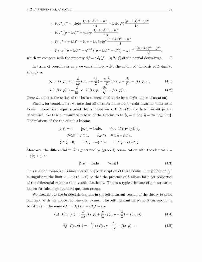
4.2 Differential Calculi 59
= (dgn)pm + (dp)gn(p+ iA)m − pm
iA+ iA(dgn)
(p+ iA)m − pmiA
= (dgn)(p+ iA)m + (dp)gn(p+ iA)m − pm
iA
= ξ ngn(p+ iA)m + (η g + iAξ g)gn(p+ iA)m − pm
iA
= ξ(ngn(p+ iA)m + gn+1 ((p+ iA)m − pm)
)+ η gn+1 (p+ iA)m − pm
iA,
which we compare with the property df = ξ ∂ξ(f) + η ∂η(f) of the partial derivatives.
In terms of coordinates x, p we can similarly write the action of the basis of L dual to
dx, η as
∂x(: f(x, p) :) =:∂
∂xf(x, p+
i~G
)− e−xG
G(f(x, p+
i~G
)− f(x, p)) :, (4.1)
∂η(: f(x, p) :) =G
i~: e−
xG (f(x, p+
i~G
)− f(x, p)) : (4.2)
(here ∂x denotes the action of the basis element dual to dx by a slight abuse of notation).
Finally, for completeness we note that all these formulae are for right-invariant differential
forms. There is an equally good theory based on L, V ∈ MHH and left-invariant partial
derivatives. We take a left-invariant basis of the 1-forms to be ξ = g−1dg, η = dp−pg−1dg.The relations of the the calculus become
[a, ξ] = 0, [a, η] = iAda, ∀a ∈ C[x]I/~,GC[p],
βR(ξ) = ξ ⊗ 1, βR(η) = η ⊗ g − ξ ⊗ p,ξ ∧ ξ = 0, η ∧ ξ = −ξ ∧ η, η ∧ η = iAη ∧ ξ.
Moreover, the differential in Ω is generated by (graded) commutation with the element θ =
−12(η + η) as
[θ, α] = iAdα, ∀α ∈ Ω. (4.3)
This is a step towards a Connes spectral triple description of this calculus. The generator 1iAθ
is singular in the limit A → 0 (~ → 0) so that the presence of ~ allows for nicer properties
of the differential calculus than visible classically. This is a typical feature of q-deformation
known for calculi on standard quantum groups.
We likewise bar the braided derivations in the left-invariant version of the theory to avoid
confusion with the above right-invariant ones. The left-invariant derivations corresponding
to dx, η in the sense df = (∂xf)dx+ (∂ηf)η are
∂x(: f(x, p) :) =:∂
∂xf(x, p) +
p
i~(f(x, p− i~
G)− f(x, p)) :, (4.4)
∂η(: f(x, p) :) = −G
~: (f(x, p− ~
G)− f(x, p)) : . (4.5)

60 Quantum Geometry of the Planck Scale Hopf Algebra
4.3 Quantum Poisson Bracket
We present in this section some elements of “quantum Poisson geometry”. We recall first
the classical situation. According to Proposition 2.3.1, any twisting of the Hopf algebra of
functions on a Lie group G by a cocycle χ admitting a reasonable expansion in a parameter
~ defines a deformation quantisation. Furthermore, the underlying Poisson bracket makes
G into a Poisson-Lie group. Note that the Poisson bracket, as with all Poisson-Lie groups,
cannot be symplectic since it must vanish at least at the group identity.
In the present case, we obtain a Poisson bracket making B+ into a Poisson-Lie group.
Proposition 4.3.1. The Poisson bracket on C(B+), for which the cocycle χ of Proposi-
tion 4.1.1 provides the quantisation, is
a, b = (e−xG − 1)
(∂a
∂x
∂b
∂p− ∂b
∂x
∂a
∂p
).
Proof. Expanding χ of Proposition 4.1.1 in ~ and expressing everything in terms of the coor-
dinates x, p yields
a • b = ab+ i~ ε(∂
∂pa(1)
)ε
(e−
xG∂
∂xb(1)
)a(2)b(2)
− i~a(1)b(1) ε
(∂
∂pa(2)
)ε
(exG∂
∂xb(2)
)+O
(~2)
= ab+ i~(e−
xG∂a
∂p
∂b
∂x− ∂a
∂p
∂b
∂x
)+O
(~2)
= ab+ i~(e−
xG − 1
)(∂a∂p
∂b
∂x
)+O
(~2),
a • b− b • a =~i
(e−
xG − 1
)(∂a∂x
∂b
∂p− ∂b
∂x
∂a
∂p
)+O
(~2).
The idea is now to take the classical Poisson bracket and apply the twisting to it in a
generalised quantum geometric setting, yielding a quantum Poisson bracket. We start by
developing an appropriate setting. We work over a general field k for this.
Since L, V ∈ HHM, we can take their arbitrary tensor powers to define tensor fields of
arbitrary mixed rank using the same correspondence with bicovariant bimodules. Thus Ω−1 =
L ⊗ H and Ω−1 ⊗H Ω−1 = L ⊗ L ⊗ H etc. We have a super-Hopf algebra T−1(Ω−1) and a
theory of twisting of quantum vector fields using the same theory of Chapter 2. Also, since
morphisms in HHM induce morphisms between bicovariant bimodules, the evaluation map
〈 , 〉 : L⊗ V → k induces the pairing between vector fields and 1-forms. Thus
Ω−1 ⊗H Ω1 → H, 〈x⊗ h, v ⊗ g〉 = 〈x, h(1) . v〉h(2)g, (4.6)

4.3 Quantum Poisson Bracket 61
Ω−1 ⊗H Ω−1 ⊗H Ω1 → Ω−1, 〈x⊗ y ⊗ h, v ⊗ g〉 = x⊗ 〈y, h(1) . v〉h(2)g, (4.7)
Ω−1 ⊗H Ω−1 ⊗H Ω1 ⊗H Ω1 → H,
〈x⊗ y ⊗ h, v ⊗ w ⊗ g〉 = 〈y, h(1) . v〉〈x, h(2) . w〉h(3)g,(4.8)
etc. The pairing L⊗L⊗V ⊗V → k in (4.8) is the natural one in a braided category, namely
to evaluate the inner L ⊗ V first and then the outer. The resulting pairing is also the same
as applying (4.7) to the first factor of Ω1⊗H Ω1 to obtain an element of Ω−1⊗H Ω1 and then
applying (4.6).
This is not the only way to formulate vector fields (for example a more left-right symmetric
way is to consider L ∈ MHH and Ω−1 = H ⊗ L, extending the pairing by 〈h ⊗ x, v ⊗ g〉 =
h〈x, v〉g), but it is the one natural in the context of the Woronowicz exterior algebra (which can
be viewed as based on a fixed identification of bicovariant bimodules with HHM (say)). Taking
now Ωn defined by quotients of V ⊗n in the exterior algebra in this approach, the natural
definition of antisymmetric vector fields is as corresponding to the appropriate subspace of
L⊗n dual to this quotient. In particular, the Poisson bivector field should be an element
Π ∈ Ω−2 = x⊗ y − ψL,L(x⊗ y)| x, y ∈ L ⊗H
since V ⊗ V is quotiented by ker(id−ψV,V ) in degree 2.
In general, we also need to impose a “Jacobi identity” on Π, which can be done as follows,
at least in the nice case where the quantum Poisson bracket is non-degenerate: We can
consider Π by the above as a map Ω1 → Ω−1 and demand that it is invertible, and that
the inverse corresponds to evaluation against some ω ∈ Ω2 which we can demand to be
closed. Alternatively, one may attempt to develop a theory of “quantum-Lie algebras” and
use the “quantum-Lie bracket” on L, thereby avoiding the invertibility assumption. This
will not be attempted here, however; for our present purposes we note that in 2 dimensions
with the classical differential calculus the Jacobi identity is redundant (similarly, every 2-
form is closed). For our particular exterior algebras the dimensions are the classical ones
(so that every 2-form is closed) and one may similarly consider any antisymmetric bivector
field as a Poisson structure. We now give the explicit form of the quantum Poisson bracket
corresponding to the above classical Poisson bracket.
Proposition 4.3.2. For the Planck scale Hopf algebra with the standard quantum differential
calculus as above, we consider Π of the form
Π = (η∗ ⊗ ξ∗ − ψL,L(η∗ ⊗ ξ∗))⊗ π(g)
for an arbitrary function π(g). Then the corresponding quantum Poisson bracket is
a, b = π(g)(aξbη − aηbξ + iA(aηbη + (aξ)ηbη − (aη)ξbη) + (iA)2(aη)ηbη
)

62 Quantum Geometry of the Planck Scale Hopf Algebra
where aξ := ∂ξa, etc. In particular, π(g) = 1G(g−1 − 1) gives the twisting of the classical
Poisson structure in Proposition 4.3.1.
Proof. We first of all use da = ξ∂ξa+ η∂ηa and the relations of the exterior algebra to obtain
da ∧ db = ξ ∧ ηf, f = aξbη − aηbξ + iA(aηbη + (aξ)ηbη − (aη)ξbη) + (iA)2(aη)ηbη.
Now the pairing can be computed as
a, b = 〈Π,da ∧ db〉 = 〈(η∗ ⊗ ξ∗ − ψ(η∗ ⊗ ξ∗))π(g), ξ ∧ ηf〉= 〈η∗ ⊗ ξ∗ − ψ(η∗ ⊗ ξ∗), ξ ⊗ π(g)(1) . η〉π(g)(2)f
= 〈η∗ ⊗ ξ∗, ξ ⊗ π(g)(1) . η − ψV,V (ξ ⊗ π(g)(1) . η)〉π(g)(2)f
= 〈η∗ ⊗ ξ∗, ξ ⊗ π(g)(1) . η − π(g)(1) . η ⊗ ξ〉π(g)(2)f = 〈η∗ ⊗ ξ∗, ξ ⊗ η〉π(g)f,
where we used functoriality of the braiding under the evaluation morphism to deduce
〈ψL,L(η∗ ⊗ ξ∗), v ⊗ w)〉 = 〈η∗ ⊗ ξ∗, ψV,V (v ⊗ w)〉
for any v, w ∈ V , and then ψV,V (ξ⊗w) = w(1) .ξ⊗w(2) = w⊗ξ since ξ is an invariant element
of the crossed module. In the last line we used g . η = η + iAξ to see that, although η is not
invariant, the evaluation 〈η∗, gn . η〉 = 〈η∗, η〉 behaves as if it is. In terms of functions a(g, p),
b(g, p) we obtain
: a(g, p) :, : b(g, p) :
= π(g) :
(g(g − 2)a(g, p) + g(
∂
∂g− 2g + 3)a(g, p+ iA) + g(g − 1)a(g, p+ 2iA)
):
• : gb(g, p+ iA)− b(g, p)
iA:
− π(g) : ga(g, p+ iA)− a(g, p)
iA: • :
(g∂
∂gb(g, p+ iA) + g(b(g, p+ iA)− b(g, p))
): .
The classical limit A→ 0 is
a(g, p), b(g, p) = π(g)g2
(∂a
∂g
∂b
∂p− ∂a
∂p
∂b
∂g
).
Thus, to get the correct Poisson structure, we need π(g) = 1G(g−1 − 1) (note that −G ∂
∂x =
g ∂∂g ).
Also, if : h :∈ C[x]I/~,GC[p] is a choice of Hamiltonian then
x = x, : h : =G
i~: (e−
xG − 1)(h(x, p+
i~G
)− h(x, p)) :, (4.9)
p = p, : h : =: −(e−xG − 1)
∂
∂xh(x, p+
i~G
)) : (4.10)

4.4 Fourier Theory 63
are the corresponding quantum Hamilton equations of motion. For a simple concrete example,
choosing the Hamiltonian h(x, p) = p2
2m + V (x) for a free particle of mass m in a potential
V (x), we obtain
x =1
2m(e−
xG − 1)(2p− i~
G), p = (e−
xG − 1)
∂
∂xV (x). (4.11)
Standard quantum mechanics (i.e. using the commutator with h) leads by contrast to
x =i
~[x, h] =
1
2m(e−
xG − 1)(2p− i~
Ge−
xG ), p =
i
~[p, h] = (e−
xG − 1)
∂
∂xV (x).
Thus the quantum Hamiltonian equations of motion reduce to the classical ones when ~→ 0
as they should, but differ from the conventional quantum mechanical equations of motion at
small momenta with Compton wavelength G. (We recall that G is the background curvature
scale.) On the other hand, the quantum Hamiltonian equations retain a full (quantum)
geometrical interpretation which is lost in conventional quantum mechanics. This suggests a
geometrical modification of conventional quantum mechanics.
4.4 Fourier Theory
In this section we make some remarks about the noncommutative Fourier theory which is
known to exist on any Hopf algebra equipped with a suitable translation-invariant integral
and a suitable coevaluation element. We recall first the general formulation, which works
basically when the Hopf algebra H is finite-dimensional, and in conventions suitable for our
particular example. Thus, we require∫
: H → k such that (∫h(1))h(2) = (
∫h)1 for all h ∈ H
(a right-integral) and∫ ∗
: H∗ → k such that φ(1)
∫ ∗φ(2) = 1
∫φ for all φ ∈ H∗ (a left-integral),
and we let∑ea ⊗ fa ∈ H ⊗ H∗ denote the canonical coevaluation element (here ea is a
basis of H and fa a dual basis). Then the Fourier transform in these conventions is
T (h) =
(∫eah
)fa, T ∗(φ) = ea
∫ ∗faφ (4.12)
and obeys
T T ∗(φ) = S−1 φ
∫ea
∫ ∗fa,
T (h(1)〈φ, h(2)〉) = T (h) S−1 φ, T ∗(〈φ(1), h〉φ(2)) = ShT ∗(φ).
(4.13)
These elementary facts are easily proven once one notes that (∫g(1)h)g(2) = (
∫gh(1))Sh(2) for
all h, g ∈ H and a similar identity on H∗. See also [KM94] for more discussion (and the
extension to braided groups).

64 Quantum Geometry of the Planck Scale Hopf Algebra
In our case the Planck scale Hopf algebra C[x]I/~,GC[p] is not finite-dimensional and there
is, moreover, no purely algebraic integral. For a full treatment one needs to introduce a Hopf-
von Neumann algebra setting along the lines in [Maj91] and work with the integral as a weight,
or one has to work with a C∗-algebra setting extended to include unbounded operators. Both
of these are nontrivial and beyond our scope here. However, the bicrossproduct form of the
Hopf algebra allows one to identify elements as normal ordered versions of ordinary functions
f(x, p) and thereby to reduce integration to ordinary integration of ordinary functions, for
any class of functions and any topological setting to which the normal ordering extends.
Therefore in this section we will initially work formally with x, p as generators (unlike the
algebraic setting in the preceding sections) and proceed to consider formal power series in
them; however, what we arrive at in this way is a well-defined deformed Fourier theory on
functions on R2 of suitably rapid decay, motivated by the Hopf algebra C[x]I/~,GC[p] and
consistent with any operator algebra setting to which normal ordering extends. This is what
we shall outline in this section.
First of all, the bicrossproduct form of the Hopf algebra implies that
∫: f(x, p) :=
∫ ∞
−∞
∫ ∞
−∞dxdp f(x, p)
is a left-integral on C[x]I/~,GC[p]. This is also evident from the explicit form of the right-
invariant derivatives (4.1) and (4.2), from which we see that the integrals of ∂x : f : and
∂η : f : vanish for suitably decaying f . On the other hand, the right-integral desired in our
preferred conventions for the Fourier theory can be similarly obtained using the left-invariant
partial differentials (4.4) and (4.5). One finds
∫: f(x, p) :=
∫ ∞
−∞
∫ ∞
−∞dxdp e
xG f(x, p), (4.14)
which is the right-integral that we shall use. (Although apparently more complicated, the
resulting Fourier theory turns out to be more computable in these conventions.)
Next, we recall from [Maj88, Maj95b] that the Planck scale Hopf algebra is essentially
self-dual. More precisely, if we let x, p be dual to the p, x generators in the sense 〈x, xnpm〉 =
i δn,0δm,1 and 〈p, xnpm〉 = i δn,1δm,0, we have an algebraic model of the dual of C[x]I/~,GC[p]
as
C[p].J 1~ ,
G~C[x] ⊆ (C[x]I/~,GC[p])∗,
where
[p, x] =i
~(1− e−x ~G ), ∆x = x⊗ 1 + 1⊗ x, ∆p = p⊗ 1 + e−x
~G ⊗ p.

4.4 Fourier Theory 65
This has the same form as C[x]I/~,GC[p], but with different parameter values and with the
opposite product and opposite coproduct. On this Hopf algebra we define normal ordering
as putting all the x to the right and the corresponding left-integral is∫ ∗
: f(p, x) :=
∫ ∞
−∞
∫ ∞
−∞dpdx ex
~G f(p, x). (4.15)
Also from the bicrossproduct form, the canonical element is [Maj95b]
∑
n,m
1
n!m! in+mxnpm ⊗ pnxm. (4.16)
Finally, we will need explicitly the actions [Maj95b]
p . f(x) = i~(e−xG − 1)
∂
∂xf, f(x) / p =
i
~(e−
~Gx − 1)
∂
∂xf (4.17)
in the bicrossproduct construction and its dual.
Proposition 4.4.1. The quantum Fourier transform on the Planck scale Hopf algebra is
T (: f(x, p) :) =
∫ ∞
−∞
∫ ∞
−∞dxdp e−i(p+ i
G)·xe−ix·(p+p.)f(x, p)
and its dual is
T ∗(: f(p, x) :) =
∫ ∞
−∞
∫ ∞
−∞dpdx e−ip·xe−ix·pf(/p+ p, x)e
~Gx,
where p. acts only on the functions in x to the right in the integral (/p acts only on functions
in x to the left).
Proof. We use the reordering equality
: f(p) :: h(x) :=: ep.· ∂
∂ph(x)f(p) :=: f(p+ p.)h(x) :
in C[x]I/~,GC[p] for functions f, h (p. only acts on functions of x). This follows from the
relation [p, f(x)] = p . f(x) for functions f(x), which is the semidirect product form of the
algebra in the bicrossproduct. Hence,
T (: f(x, p) :) =∑
n,m
1
n!m! in+mpnxm
∫xnpm : f(x, p) :
=∑
n,m
1
n!m! in+mpnxm
∫: xn(p+ p.)mf(x, p) :
=∑
n,m
1
n!m! in+mpnxm
∫dxdp e
xGxn(p+ p.)mf(x, p)
=
∫dxdp e−i(p+ i
G)·xe−ix·(p+p.)f(x, p),

66 Quantum Geometry of the Planck Scale Hopf Algebra
where p. only acts in the powers of x to its right. In C[p]I/ 1~ ,
G~C[x] we have similarly
: f(x) :: h(p) :=: f(x)e/p· ∂
∂ph(p) :=: f(x)h(/p+ p) : .
Hence,
T ∗(: f(p, x) :) =∑
n,m
1
n!m! in+mxnpm
∫ ∗pnxm : f(p, x) :
=∑
n,m
1
n!m! in+mxnpm
∫ ∗: pnxmf(/p+ p, x) :
=∑
n,m
1
n!m! in+mxnpm
∫dpdx pnxmf(/p+ p, x)e
~Gx
=
∫dpdx e−ip·xe−ix·pf(/p+ p, x)e
~Gx.
From the properties of the Fourier transform, we see in particular that it turns the (left-
invariant) derivatives ∂x and ∂η in (4.4)–(4.5) into multiplication by the corresponding el-
ement of the dual. Also, these derivatives become right-handed derivatives ∂x and ∂η on
C[p]I/ 1~ ,
G~C[x] by identifying it with the opposite algebra and coalgebra to C[x].J 1
~ ,G~C[p] and
making the corresponding notational and parameter changes.
Proposition 4.4.2.
T (∂xa) = T (a)ipe~Gx, T (∂ηa) = T (a)
iG
~(e~Gx − 1),
T ∗(∂xφ) = ipexGT ∗(φ), T ∗(∂ηφ) = iG(e
xG − 1)T ∗(φ),
T T ∗(φ) = (2π)2 S−1 φ.
Proof. This is a short computation to identify the partial derivatives as ∂x(a) = a(1)〈−ip, a(2)〉and ∂η(a) = a(1)〈 iG~ (e−
~Gx−1), a(2)〉, i.e. to identify the corresponding elements of L. Similarly,
∂x corresponds to −ip and ∂η corresponds to iG(e−xG − 1) via the right coregular action. One
can then verify the analogue of (4.13) directly in our setting for functions of suitably rapid
decay.
Note that when we take the limit ~ → 0 the Hopf algebra C[p]I/ 1~ ,
G~C[x] becomes U(b+)
or κ-Minkowski space [MR94] with the relations
[p, x] =i
Gx
(i.e. κ = Gi ) regarded as a noncommutative space. Thus,

4.4 Fourier Theory 67
Corollary 4.4.3. In the classical limit ~→ 0 the Fourier transform becomes
T : C(B+)→ U(b+), T (: f(x, p) :) =
∫ ∞
−∞
∫ ∞
−∞dxdp e−i(p+ 1
κ)·xe−ix·pf(x, p),
T ∗ : U(b+)→ C(B+), T ∗(: f(p, x) :) =
∫ ∞
−∞
∫ ∞
−∞dpdx e−ip·xe−ix·pf(/p+ p, x)
with f(x) / p = − xκ∂∂xf . Moreover,
T (∂xa) = T (a)ip, T (∂ηa) = T (a)ix,
∂x(: f(x, p) :) =:∂
∂xf(x, p) +
ip
κ
∂
∂pf(x, p) :, ∂η(: f(x, p) :) =:
∂
∂pf(x, p) : .
The intertwiner properties of T ∗ in this limit are read off from Proposition 4.4.2 while
required right-derivatives simplify to
∂x(: f(p, x) :) =:∂
∂xf(p, x) :, ∂η(: f(p, x) :) =: −κ(f(p− 1
κ, x)− f(p, x)) : . (4.18)
We also have a dual limit ~,G → ∞ with Gi~ = κ constant, where C[x]I/~,GC[p] becomes
U(b−) (with the opposite Lie algebra to b+) and C[p]I/ 1~ ,
G~C[x] becomes C(B−). We regard
the former as another version of κ-Minkowski space (with opposite commutation relations).
Corollary 4.4.4. In the limit ~,G→∞ with Gi~ = κ the Fourier transform becomes
T : U(b−)→ C(B−), T (: f(x, p) :) =
∫ ∞
−∞
∫ ∞
−∞dxdp e−ip·xe−ix·(p+p.)f(x, p),
T ∗ : C(B−)→ U(b−), T ∗(: f(p, x) :) =
∫ ∞
−∞
∫ ∞
−∞dpdx e−ip·(x+ 1
κ)e−ix·pf(p, x)
with p . f(x) = − 1κ∂∂xf . Moreover,
T ∗(∂xφ) = ipT ∗(φ), T ∗(∂ηφ) = ixT ∗(φ),
∂x(: f(x, p) :) =:∂
∂xf(x, p) +
ip
κ
∂
∂pf(x, p) :, ∂η(: f(x, p) :) =:
∂
∂pf(x, p) : .
In this limit the intertwiner properties of T do not simplify (we refer to Proposition 4.4.2),
but the corresponding derivatives become
∂x(: f(x, p) :) =:∂
∂xf(x, p) :, ∂η(: f(x, p) :) =: −κ(f(x, p− 1
κ)− f(x, p)) : . (4.19)
Therefore we obtain in fact two versions of Fourier theory on κ-Minkowski space as two
limits of Fourier theory on the Planck scale Hopf algebra. This Hopf algebra, being of self-
dual form, has the power to become both a classical but curved phase space (the classical
limit) and its dual (the second limit), in addition to the flat space quantum mechanics limit.

68 Quantum Geometry of the Planck Scale Hopf Algebra
There are many further possible developments of the geometry and Fourier theory on
the noncommutative phase space in this toy model of Planck scale physics, among them
quantum field theory (second quantisation) in a first-order formalism. There is also a physical
interpretation of the self-duality as an observable-state duality [Maj88, Maj95a] which should
be related to the noncommutative geometric picture above. Finally, we note that there
are higher dimensional models of the bicrossproduct form [Maj90a, Maj91] which could be
investigated from a similar point of view. These are some directions for further work.

Chapter 5
Spin and Statistics
While spin in quantum physics arises from the geometry of space-time, statistics is connected
to the geometry of configuration space. Half-integer spin and Bose-Fermi statistics arise in 3
or higher dimensions, while in 2 dimensions more general fractional spin and anyonic statistics
are possible (see [Wil90] and references therein). In fact, both, spin and statistics are related
to symmetries. In the case of spin this is plainly understood in terms of the symmetries
of space-time. In the case of statistics the link is more indirect. From the geometry of a
configuration space of identical particles [LM77] one is led (in the general case) to the braid
group, which acts on it by particle exchange [Wu84]. From the representation theory of the
braid group one naturally arrives at the concept of braided categories to describe statistics.
While foreign to ordinary quantum field theory, such a general formulation of statistics has
already been incorporated into algebraic quantum field theory [FRS89, FG90]. Going further,
a reconstruction theorem of quantum group theory tells us that (essentially) every braided
category is the category of representations of a quantum group. Thus, for any braid statistics
there is a quantum group symmetry of the theory that generates the statistics. The relevant
quantum groups for anyonic statistics are known [Maj93a, Maj95b].
After reviewing these facts, we ask, in this chapter, the natural question of whether
and how the (quantum) group symmetries behind spin and statistics are related. Such a
connection should be expected in the Bose-Fermi case from the spin-statistics theorem [Fie39,
Pau40]. In this case, both groups generating spin and statistics turn out to be (essentially) Z2.
Remarkably, the statement of the spin-statistics theorem is found to be precisely equivalent to
the requirement that the groups be identified. This leads to a quantum symmetry group that
encodes (a) the space-time symmetries, (b) the statistics, and (c) the spin-statistics theorem.
Technically, this quantum group is the ordinary space-time symmetry (e.g., Poincare) group
as a Hopf algebra, but equipped with a non-trivial coquasitriangular structure. We proceed
to explore the possible relations of spin and statistics in the more general case of fractional
69

70 Spin and Statistics
spin and anyonic statistics. This amounts (under certain restrictions) to a classification of
all possible spin-statistics theorems which could be implemented by a unified quantum group
symmetry.
It is essential for our treatment to work with quantum groups of function algebra type
and not of enveloping algebra type. The global structure of the (quantum) groups, not visible
in the enveloping algebra setting, is crucial in the unified description of spin and statistics. In
an enveloping algebra setting one would have to provide the global information “by hand”,
i.e., by adjoining elements.
Much of the chapter (Sections 5.1–5.4) is devoted to a coherent review of geometrical as-
pects of spin and statistics. Section 5.1 reviews the geometrical origin of spin while Section 5.2
that of particle exchange statistics. The description of statistics in terms of braided categories
is introduced in Section 1.2.1 and the quantum symmetries underlying anyonic statistics are
identified in Section 5.4. This finally enables us in Section 5.5 to investigate the unification
of the symmetries of spin and statistics.
We work over the complex numbers throughout this chapter.
5.1 Spin
We start by recalling the geometric origin of spin. In classical mechanics we require that ob-
servable quantities form a representation of the symmetry group of space-time. In quantum
mechanics it is only required that such a representation is projective, i.e., it is a represen-
tation “up to a phase” [Wey31]. However, projective representations of a Lie group are in
correspondence to ordinary representations of its universal covering group [Bar54].
Suppose we have some connected orientable (pseudo-) Riemannian space-time manifold
M . We denote its principal bundle of oriented orthonormal frames by (E,M,G), where E
is the total space and G the structure group, i.e., the orientation preserving isotropy group.
If M has signature (n,m) then G = SO(n,m). Let G be the universal covering group of
G. Denote by (E,M, G) the induced lift of (E,M,G) (assuming no global obstructions).1
Given a representation of G with label j, a field with spin j is described by a section of the
corresponding bundle associated with (E,M, G). If j labels a representation of G itself, we
say that the spin is “integer”, otherwise “fractional”. Consider the exact sequence
π1(G) → G G, (5.1)
1Strictly speaking, we should consider coverings of the global symmetry group. However, if M is a Rieman-
nian homogeneous space, E can be identified with the global isometry group and E with its universal cover
(assuming M to be simply connected).

5.2 Statistics 71
where π1(G) denotes the fundamental group of G. A representation of G is a representation of
G if and only if the induced action of π1(G) is trivial. Thus, loosely speaking, the “fractions”
of spin are labeled by the irreducible representations of π1(G). In our present context (we
assume at most one time direction) there arise only two different cases which we review in
the following.
Let M be 3-dimensional Euclidean space. Then G = SO(3) and the exact sequence (5.1)
becomes
Z2 → SU(2) SO(3). (5.2)
With the usual conventions, irreducible representations of SU(2) are labeled by half-integers
and those with an integer label descend to representations of SO(3). Z2 has just two in-
equivalent irreducible representations that distinguish between the two choices, integer or
non-integer. More generally, π1(SO(1, n)) = π1(SO(n)) = Z2 for all n ≥ 3. Thus, if the
dimension of space is ≥ 3 we can only have integer and half-integer spins.
Now, let M be 2-dimensional Euclidean space. We obtain the exact sequence
Z → R SO(2). (5.3)
Since the groups are abelian, their unitary irreducible representations form themselves (abelian)
groups. In fact these are SO(2), R, and Z. (The sequence (5.3) is Pontrjagin self-dual.)
Thus, the unitary irreducible representations of R are labeled by real numbers and descend
to SO(2) if the label is integer. The “fractional” part is labeled by U(1) = SO(2). Since also
π1(SO(1, 2)) = Z, we conclude that in 2 spatial dimensions continuous real spin is allowed.
Finally, the case of one spatial dimension is degenerate since the orientation preserving
spatial isotropy group is trivial. We do not discuss this case further.
5.2 Statistics
In the following we review the various possibilities for exchange statistics arising from the
quantisation of a system of identical particles [LM77, Wu84]. We consider particles in d-
dimensional Euclidean space. Naively, the configuration space for N particles is RdN . How-
ever, due to the particles being identical, configurations which differ only by a permutation of
the particle positions are to be considered identical. Furthermore, we exclude the singularities
arising from the subspace D ⊂ RdN where two or more particle positions coincide. Thus, the
true configuration space is (RdN −D)/SN , where SN denotes the symmetric group acting by
exchanging the particle positions. For more than one particle and more than one dimension
it is multiply connected.

72 Spin and Statistics
γii i+ 1
Figure 5.1: Clockwise exchange of particle i with particle i+ 1.
i i+ 1
i+ 1 i
i i+ 1
i+ 1 i
γi γ−1i
Figure 5.2: Braid generators γi and γ−1i in diagrammatic notation.
Assuming no internal structure for the particles, quantisation can now be performed by
constructing a complex line bundle with flat connection over this configuration space. The
wave-function is then a section of this bundle. If we parallel transport along a non-contractible
loop γ in configuration space, the wave-function picks up a phase factor χ(γ) coming from
the holonomy of the connection. This defines a one-dimensional unitary representation of the
fundamental group of the configuration space. (Note that this excludes parastatistics here.)
For dimension d = 2, the fundamental group of the configuration space is the braid group
on N elements, BN . It is generated by elements γ1, . . . , γN−1 with relations γiγj = γjγi for
i− j 6= ±1 and
γiγi+1γi = γi+1γiγi+1. (5.4)
To understand this more concretely, consider the inequivalent ways of exchanging two par-
ticles in the plane without coincidence. They correspond to non-contractible loops in the
configuration space and thus to elements of its fundamental group. Indeed, γi corresponds
to the exchange of particle i and particle i + 1 in (say) clockwise direction, see Figure 5.1.
We represent this by a diagram which can be thought of as depicting the particle trajectories
(moving from top to bottom) as they exchange, see Figure 5.2. A counter-clockwise exchange
corresponds to the inverse γ−1i . We can also wind the particles around each other more than
once, corresponding to powers of γi or its inverse. Figure 5.3 shows the braid relation (5.4)
in diagrammatic notation.
The one-dimensional unitary representations of the braid group are labeled by an angle θ

5.3 Braided Categories and Statistics 73
=
Figure 5.3: Braid relation in diagrammatic notation.
and take the form
χ(γi) = eiθ ∀i. (5.5)
This was termed θ-statistics in [Wu84]. More generally, a statistics that is induced by repre-
sentations of the braid group is called a braid statistics.
In dimension d ≥ 3, the fundamental group of the configuration space is just the symmetric
group SN . It can be obtained from the braid group by imposing the extra relations γi =
γ−1i . The geometric meaning of this is that the clockwise and counter-clockwise exchange of
particles are equivalent (homotopic), since we can use the extra dimensions to deform one path
into the other. Diagrammatically, over- and under-crossings (Figure 5.2) become equivalent.
The possible representations (5.5) reduce to just two: bosonic (θ = 0) and fermionic (θ = π)
statistics.
5.3 Braided Categories and Statistics
In quantum field theory, multi-particle states are usually expressed in a Fock space formalism.
That is, they are tensor products of one-particle states. In order to describe a general braid
statistics in this context, we define invertible linear maps
ψ : V ⊗W →W ⊗ V
that exchange particles in state spaces V and W , and represent the elements γi of the braid
group. ψ is called a braiding. We depict it by the same crossing diagram that we used for γi
(Figure 5.2). The diagram is now interpreted as a map, to be read from top to bottom, where
the strands carry the vector spaces V and W respectively (Figure 1.1). In this formulation,
we can easily express the statistics between different particles as well, by defining ψ for V
and W being different spaces. Also, we are not restricted to one-dimensional representations
of the braid group (or symmetric group) as was the discussion in Section 5.2. Furthermore,
we can extend ψ to tensor products of multi-particle states by composing in the obvious way
(Figure 1.2). In fact, we can forget about the origin from the braid group or symmetric group

74 Spin and Statistics
altogether if we implement the constraints corresponding to their relations. For the braid
group this is the braid relation, expressed by the diagram in Figure 5.3, which is now an
identity between maps on three-fold tensor products. For the symmetric group we have the
additional constraint that ψ and its inverse must be identical, i.e., diagrammatically over-
and under-crossings are identified.
If ψ takes the special form
ψ(v ⊗ w) = qw ⊗ v. (5.6)
with q ∈ C∗ it is called an anyonic statistics, since particles obeying such statistics are called
anyons [Wil82]. If V and W are state spaces of identical particles without internal structure
we recover θ-statistics (5.5) with q = eiθ. (Note that we allow θ to be complex here.) The
general expression for Bose-Fermi statistics in this formulation is
ψ(v ⊗ w) = (−1)|v|·|w|w ⊗ v, (5.7)
where |v| = 0 for bosons and |v| = 1 for fermions.
In fact, what we have described here is nothing but a braided category as introduced in
Section 1.2.1. Note that the braid relation (Figure 5.3) follows from Definition 1.2.3.
A description of statistics by braided categories was first employed in the context of
algebraic quantum field theory [FRS89, FG90]. However, it can also be integrated into a
(generalised) path integral formulation of quantum field theory. This will be the object of
Chapter 6.
5.4 Quantum Groups and Statistics
How do quantum groups come into the game? We recall from Section 1.2 that certain mod-
ule categories of quantum groups are naturally equipped with a braiding, i.e., are naturally
braided categories. In particular, this is true for the category of comodules of a coquasitri-
angular Hopf algebra, see (1.8). This generalises the situation for representations of ordinary
groups which come canonically equipped with the trivial braiding τ : V ⊗W →W⊗V defined
by the exchange v ⊗ w 7→ w ⊗ v, and induced from the trivial coquasitriangular structure
R = ε⊗ ε.Remarkably, the converse is also true: Given a braided category, we can (under cer-
tain technical conditions) reconstruct a quantum group (coquasitriangular Hopf algebra) so
that the given category arises as its category of representations (comodules). This is called
Tannaka-Krein reconstruction, see [Maj95b].
Having seen that braided categories can be used to describe statistics, we can say that
quantum group theory naturally integrates the notions of “spin” (representation theory) and

5.4 Quantum Groups and Statistics 75
quantum group R U(1) Zn Z2
representation labels R Z Zn Z2
statistics parameter q ∈ C∗ q ∈ C∗ qn = 1 q = −1
Table 5.1: Anyonic statistics generating quantum groups.
statistics. More precisely, the reconstruction theorem tells us that for a given braid statistics
(given by a braided category) there is an underlying symmetry quantum group, so that
the statistics of particles is determined by their representation labels. In the following, we
discuss this for anyonic statistics including the special case of Bose-Fermi statistics. The
relevant quantum groups were identified by Majid [Maj93a, Maj95b] (in a dual formulation
of enveloping algebras).
The quantum group generating general anyonic statistics turns out to be the ordinary
group U(1), but with a non-standard coquasitriangular structure. As a quantum group it
is the function algebra C(U(1)). A natural basis in terms of the coproduct are the Fourier
modes fk : φ 7→ e2πikφ, labeled by k ∈ Z. The relations are fkfl = fk+l, the coproduct is
∆ fk = fk⊗fk, the counit is ε(fk) = 1, and the antipode is S fk = f−k. The coquasitriangular
structure R : C(U(1))⊗ C(U(1))→ C that generates the braiding is given by
R(fk ⊗ fl) = qkl. (5.8)
The unitary irreducible representations of U(1) are labeled by k ∈ Z. The braid statistics
takes the form
ψ(vk ⊗ vl) = qklvl ⊗ vk. (5.9)
This reduces to expression (5.6) for particles in the representation k = l = 1.
As it will be of relevance later, we remark that the same anyonic statistics can also be
generated by the group R. As a quantum group we consider the function algebra C(R)
generated by the periodic functions. The only difference to the U(1) case discussed above is
that the basis fk is now labeled by real numbers k ∈ R and not just integers. Otherwise the
algebraic structure is the same and (5.8) and (5.9) still hold in the same form. Representations
are also labeled by k ∈ R now.
For q = eiθ an n-th root of unity, we call the statistics rational since θ/2π is rational. In
this case we can restrict U(1) to the subgroup Zn. This corresponds in the quantum group
setting to the extra relations fk = fk+n, so that we obtain a finite dimensional quantum group.
Irreducible representations are now labeled by k ∈ Zn. However, it will be convenient for the
following discussion to introduce an alternative fractional labeling by k ∈ 1nZn. Expression

76 Spin and Statistics
(5.9) is thus modified to
ψ(vk ⊗ vl) = qn2klvl ⊗ vk. (5.10)
Expression (5.6) is recovered for k = l = 1n . The special case of Z2 (θ = π) is Bose-Fermi
statistics (5.7) with |v0| = 0 and |v 12| = 1.
The quantum groups generating anyonic statistics are summarised in Table 5.1 (with the
special case of Z2 listed separately).
5.5 Unifying Spin and Statistics
Having found an underlying “spin” connected with statistics, the natural question arises what
possible relation it can have to the geometric spin discussed in Section 5.1. This is in essence
the question of what spin-statistics theorems are quantum geometrically realisable. We give
a complete answer to this question in the following (under the restricting assumption that
integer spin particles behave bosonic in dimension ≥ 3).
We consider first the Bose-Fermi case. Our labelling of the Z2 representations above by
0, 12 is already suggestive of an interpretation as the fractional part of geometric spin. The
latter is also described by a Z2, arising from the universal covering of the isotropy group in
dimensions ≥ 3. And in fact, identifying the two groups is precisely equivalent to requiring
the usual spin-statistics theorem to hold.
To make this more precise we consider the generic case of 3-dimensional Euclidean space.
Translating the exact sequence (5.2) into quantum group language, it takes the arrows reversed
form2
C(SO(3)) → C(SU(2)) C(Z2). (5.11)
Instead of inheriting the trivial coquasitriangular structure canonically associated to ordinary
groups, we equip C(Z2) with the non-trivial coquasitriangular structure generating the Bose-
Fermi statistics. This induces a non-trivial coquasitriangular structure on C(SU(2)) which
precisely exhibits the usual spin-statistics relation. Explicitly, for a group-like basis 1, g of
C(Z2) and a Peter-Weyl basis tlij, l ∈ 12N0 of C(SU(2)), the right hand map of (5.11) is
tlij 7→ δijg2l. The coquasitriangular structure R(g ⊗ g) = −1 on C(Z2) pulls back to
R(tlij ⊗ tmkl) = (−1)4lmδijδkl
on C(SU(2)). This induces the braiding
ψ(vk ⊗ vl) = (−1)4klvl ⊗ vk,2Note that this is not an exact sequence of vector spaces.

5.5 Unifying Spin and Statistics 77
relating spin and statistics for bosons and fermions in the familiar way. The analogous
construction can be made in any space-time with spatial dimension≥ 3, since the only relevant
input is that the fundamental group of the isotropy group is Z2. This ensures that the function
algebra of the covering group is Z2-graded into functions that are symmetric or antisymmetric
with respect to exchange of the sheets. This decomposition is also a decomposition into
subcoalgebras. Thus, the covering group admits the coquasitriangular structure
R(f ⊗ g) = (−1)|f |·|g| ε(f) ε(g).
Note that we can further pull the coquasitriangular structure back to the relevant global
space-time symmetry group by the same argument. For a treatment of Bose-Fermi statistics
in 2 dimensions see the discussion below.
We now proceed to the more complicated case of anyonic statistics. Although we can
embed U(1) into SU(2), the coquasitriangular structure (5.8) does not pull back from C(U(1))
to C(SU(2)). The same is true for the other spin-groups. (This is easily seen by embedding
through an intermediate SU(2).) Consequently, we cannot relate the statistical “spin” of
anyonic statistics to geometric spin in dimension 3 or higher. Even in the rational case this
is only possible for q = ±1, which is the Bose-Fermi case described above. Thus, we must
restrict to 2 dimensions, where the covering of the spatial isotropy group is described by the
exact sequence (5.3). In contrast to the Bose-Fermi case the statistical group U(1) is different
from the group Z describing the covering. However, we can use the group R to generate
the statistics instead (see Table 5.1) and identify it directly with the universal cover R of the
isotropy group. We obtain a spin-statistics relation between anyonic statistics and continuous
geometric spin. However, for q 6= 1 we never have the property that representations which
descend to the isotropy group have bosonic statistics, i.e., trivial braiding with all other
representations.
We can implement this property, however, if we only consider a finite covering of the
isotropy group. This leads to the exact sequence
Zn → SO(2) SO(2)
instead of (5.3). The spins are restricted from continuous values to n-th fractions. We
can now establish a spin-statistics relation by identifying the Zn of the covering with the
Zn of rational anyonic statistics. The braiding is the one described by (5.10). Pullback
from C(Zn) to C(SO(2)) corresponds to extending the representation labels from 1nZn to 1
nZ.
Representations of the covering SO(2) that descend to representations of the covered SO(2)
are precisely the ones that are bosonic, i.e., have trivial braiding with all other representations.
n = 2 is the Bose-Fermi case.

78 Spin and Statistics
spatial dimension 2 2 ≥ 3
statistics quantum group R Zn Z2
statistics parameter q ∈ C∗ qn = 1 q = −1
integer spin bosonic − √ √
Table 5.2: Possible spin-statistics relations.
Conversely, we may ask the question what possible statistics can be attached to the
geometric spin, i.e., which coquasitriangular structure is admitted by the relevant (quantum)
group. Its turns out that all the relevant groups are abelian. A coquasitriangular structure on
the function Hopf algebra of an abelian group is a bicharacter on its Pontrjagin dual, i.e., its
group of unitary irreducible representations. In dimension 3 or higher, if we require bosonic
statistics for representations descending to the isotropy group, any braiding must be induced
by C(Z2) in (5.11). The dual of Z2 is Z2 and there are only two bicharacters on it: The
trivial one (purely bosonic statistics) and the Bose-Fermi one discussed. In 2 dimensions, the
covering group R of the isotropy group is self-dual and any bicharacter corresponds to (5.8)
for some q ∈ C∗. We also see the reason now why we were not able to induce the braiding from
Z: Its dual is U(1) which has only the trivial bicharacter. In 2 dimensions with finite covering
the relevant group is Zn. It is self-dual and the bicharacters correspond to the different n-th
roots of unity leading to rational anyonic statistics. Thus, our above discussion has already
exhausted the possibilities of attaching statistics to spin. Table 5.2 gives a summary.
Of course, even in the absence of a spin-statistics relation we can encode the space-time
symmetries as well as the statistics in terms of just one symmetry (quantum) group. This is
then simply the product of the two relevant (quantum) groups.
We make a remark on a geometric explanation of a spin-statistics connection in terms
of a rotation. The usual argument (in simplified form) is that rotating two particles about
their common center should yield the same phase as the statistical exchange. For general
anyonic spin one would thus expect a factor of qk+l
2 for particles of spin k and l. This does
not in general define a consistent braid statistics, however. The only case in which it does is
Bose-Fermi statistics of identical particles (k = l). In this case we have the “accident” that
(−1)4l2 = (−1)2l for l ∈ 12N0. One could perhaps try to rescue the argument by saying that
it is only valid for “elementary” particles and that the different results for higher spin come
from “compositeness”.

Chapter 6
Braided Quantum Field Theory –
Foundations
If we want to realise the promise that quantum geometry appears to hold for physics, we
have to generalise our physical theories. More precisely, this means extending the ordinary
differential geometric notions on which they are built to quantum geometric ones. For funda-
mental physical theories this certainly includes quantum field theory with its notion of group
symmetry. In other words, we need to extend the framework of quantum field theory to one
that admits not only ordinary groups but quantum groups as symmetries.
As discussed in the previous chapter, situations arise where particles obey a more general
kind of statistics than Bose or Fermi. To formulate quantum field theories involving such
particles, it is desirable to extend the usual commutator/anticommutator formalism to a
more general one capable of describing general braid statistics.
In fact, both objectives can be addressed at the same time. This is the subject of the
present chapter. We introduce a generalisation of quantum field theory that admits quantum
group symmetries as well as braid statistics. This is achieved by the transition from ordinary
to braided categories, hence the name braided quantum field theory.
We follow the path integral approach, going from (braided) Gaussian path integrals via
perturbation theory to Feynman diagrams. In the braided setting this procedure naturally
leads us to generalised Feynman diagrams that are braid diagrams, i.e., they have nontrivial
over- and under-crossings. In view of Chapter 5 the crossings have a natural interpretation in
terms of particle exchanges. We consider the special cases of bosonic and fermionic statistics
where we recover the results of quantum field theory in its standard formulation.
Section 6.1 introduces the braided path integral. We start by defining Gaussian integrals
on braided spaces based on [Maj93b, KM94]. We obtain a braided generalisation of Wick’s
79

80 Braided Quantum Field Theory – Foundations
theorem that tells us how free 2n-point functions decompose into propagators. It is shown
that for the cases of bosonic and fermionic statistics the braided path integral reproduces the
ordinary path integrals with commuting and anticommuting variables respectively.
We consider interactions in Section 6.2 and develop perturbation theory along the lines
of ordinary quantum field theory. This leads us to braided Feynman diagrams by building
on the diagrammatic language of braided categories. The ordinary Feynman rules for bosons
and fermions are recovered for bosonic and fermionic statistics respectively.
6.1 The Braided Path Integral
6.1.1 Gaussian Integration
The calculus of differentiation and Gaussian integration on braided spaces that we build on
was developed by Majid [Maj93b] and Kempf and Majid [KM94] in an R-matrix setting.
However, we need a more abstract and basis free formulation of their formalism so that we
redevelop the notions here. Furthermore, our Theorem 6.1.1 goes beyond their result [KM94,
Theorem 5.1].
We require the concept of a rigid braided category (see the references mentioned at the end
of Section 1.2.1). This means, that we have for every object X in the category a dual object
X∗ and morphisms ev : X⊗X∗ → k (evaluation) and coev : k→ X∗⊗X (coevaluation) that
compose to the identity on X and X∗ in the obvious ways.
Now, suppose we have some rigid braided category B and a vector space X ∈ B. Essen-
tially, we want to define the (normalised) integral of functions α in the “coordinate ring” on
X multiplied by a Gaussian weight function w, i.e., we want to define
Z(α) :=
∫αw∫w. (6.1)
First, we need to specify this “coordinate ring”. We identify the dual space X∗ ∈ B as
the space of “coordinate functions” on X. This corresponds to the situation in Rn where
a coordinate function is just a linear map from Rn into the real numbers. The polynomial
functions on X are naturally elements of the free unital tensor algebra over X∗,
X∗ :=∞⊕
n=0
X∗n, with X∗0 := 1 and X∗n := X∗ ⊗ · · · ⊗X∗︸ ︷︷ ︸n times
,
where 1 is the one-dimensional space generated by the identity. 1 plays the role of the constant
functions and the tensor product corresponds to the product of functions. X∗ naturally has
the structure of a braided Hopf algebra (a Hopf algebra in a braided category, see [Maj95b])

6.1 The Braided Path Integral 81
via
∆ a = a⊗ 1 + 1⊗ a, ε(a) = 0, S a = −a
for a ∈ X∗ and ∆, ε,S extend to X∗ as braided (anti-)algebra maps. This encodes translations
on X.
To make the notion of “coordinate ring” more precise, one could perhaps consider a kind
of symmetrised quotient of X∗ in analogy with the observation that coordinates commute in
ordinary geometry. There seems to be no obvious choice for such a quotient in the general
braided case. Remarkably, however, such a choice is not necessary. In fact, the following
treatment is entirely independent of any relations, as long as they preserve the (graded)
braided Hopf algebra structure.
The next step is the introduction of differentials [Maj93b]. The space of coordinate dif-
ferentials should be dual to the space X∗ of coordinate functions. We just take X itself and
define differentiation on X∗ by the pairing ev : X⊗X∗ → k in B. To extend differentiation to
the whole “coordinate ring” X∗, we note that the coproduct encodes coordinate translation.
This leads to the natural definition that
diff := (ev⊗ id) (id⊗∆) : X ⊗ X∗ → X∗
is differentiation on X∗. Here, ev is the trivial extension of ev to X⊗X∗ → k, i.e., ev |X⊗X∗n =
0 for n 6= 1. We also use the more intuitive notation ∂(a) := diff(∂⊗a) for ∂ ∈ X and a ∈ X∗.Let ∂ ∈ X and α, β ∈ X∗. The definition of ev gives at once
ev(∂ ⊗ αβ) = ev(∂ ⊗ α) ε(β) + ev(∂ ⊗ β) ε(α).
Using that the coproduct is a braided algebra map, we obtain the braided Leibniz rule
∂(αβ) = ∂(α)β + ψ−1(∂ ⊗ α)(β). (6.2)
Iteration yields
∂(α) = (ev⊗ idn−2)(∂ ⊗ [n]ψ α),
where n is the degree of α and [n]ψ : X∗n → X∗n with
[n]ψ := idn +ψ ⊗ idn−2 + · · ·+ ψn−2,1 ⊗ id +ψn−1,1
is a braided integer. We adopt the convention of writing ψn,m for the braiding between X∗n
and X∗m (respectively ψ−1n,m for the inverse braiding).

82 Braided Quantum Field Theory – Foundations
As in [KM94], we view the Gaussian weight w formally as an element of X∗ and define
its differentiation via an isomorphism
γ : X → X∗ so that ∂(w) = −γ(∂)w for ∂ ∈ X. (6.3)
This expresses the familiar notion that differentiating a Gaussian weight yields a coordinate
function times the Gaussian weight. γ should accordingly be thought of as defining a braided
analogue of the quadratic form in the exponential of the weight.
Also familiar from ordinary Gaussian integration is the fact that integrals of total differ-
entials vanish. That is, we require∫∂(αw) = 0 for ∂ ∈ X,α ∈ X∗. (6.4)
It turns out that the three rules (6.2), (6.3), and (6.4) completely determine the integral (6.1).
Remarkably, the statement that the Gaussian integral of a polynomial function can be
expressed solely in terms of Gaussian integrals of quadratic functions still holds true in the
braided case. This generalises what is known in quantum field theory as Wick’s theorem. To
state it, we need another set of braided integers [n]′ψ : X∗n → X∗n with
[n]′ψ := idn + idn−2⊗ψ−1 + · · ·+ ψ−11,n−1, (6.5)
which are related to the original ones by [n]′ψ = ψ−11,n−1[n]ψ. We also require the corresponding
braided double factorials [2n− 1]′ψ!! : X∗2n → X∗2n with
[2n− 1]′ψ!! := ([1]′ψ ⊗ id2n−1) ([3]′ψ ⊗ id2n−3) · · · ([2n− 1]′ψ ⊗ id). (6.6)
Theorem 6.1.1 (Braided Wick Theorem).
Z |X∗2 = ev ψ (id⊗γ−1), (6.7)
Z |X∗2n = (Z |X∗2)n [2n− 1]′ψ!!, Z |X∗2n−1 = 0, ∀n ∈ N. (6.8)
Proof. For α ∈ X∗ and a ∈ X∗ we have
αaw = −α diff(γ−1(a)⊗ w) = −diff(ψ(α⊗ γ−1(a))w) + (diff ψ(α⊗ γ−1(a)))w,
using the differential property (6.3) of w and the braided Leibniz rule (6.2). Applying Z, we
can ignore the total differential and obtain
Z(αa) = Z(diff ψ(α⊗ γ−1(a))). (6.9)
This gives us immediately
Z(a) = 0 and Z(ab) = ev ψ(a⊗ γ−1(b))

6.1 The Braided Path Integral 83
for b ∈ X∗. We rewrite (6.9) to find
Z |X∗n = Z |X∗n−2 diff (γ−1 ⊗ idn−1) ψn−1,1
= Z |X∗n−2 (ev⊗ idn−2) (γ−1 ⊗ [n− 1]ψ) ψn−1,1
= (ev⊗Z |X∗n−2) (γ−1 ⊗ [n− 1]ψ) ψn−1,1
= (ev⊗Z |X∗n−2) ψn−1,1 ([n− 1]ψ ⊗ γ−1)
= (Z |X∗2 ⊗Z |X∗n−2) (id⊗ψn−2,1) ([n− 1]ψ ⊗ id)
= (Z |X∗n−2 ⊗Z |X∗2) ψ−12,n−2 (id⊗ψn−2,1) ([n− 1]ψ ⊗ id)
= (Z |X∗n−2 ⊗Z |X∗2) (ψ−11,n−2 ⊗ id) ([n− 1]ψ ⊗ id)
= (Z |X∗n−2 ⊗Z |X∗2) ([n− 1]′ψ ⊗ id),
which gives us a recursive definition of Z leading to the formulas stated.
6.1.2 Path Integration
Let us rephrase and explain the result in a more familiar notation. To simplify, we consider
Gaussian integration with a finite basis φ1, φ2, . . . of the space X∗ of coordinate functions.
The (free) n-point function can be written as1
〈φk1φk2 · · ·φkn〉 := Z(φk1φk2 · · ·φkn) =
∫Dφφk1φk2 · · ·φkn exp(−S(φ))∫
Dφ exp(−S(φ)). (6.10)
This is to be compared with (6.1), setting w(φ) = exp(−S(φ)) and α(φ) = φk1φk2 · · ·φkn . We
also introduce differentials ∂1, ∂2, . . . forming a basis of X dual to the coordinate functions.
The integration rule (6.4) now takes the form
∫Dφ∂i(φk1 · · ·φkn exp(−S)) = 0. (6.11)
Note that exp(−S(φ)) can not necessarily be given the meaning of an ordinary exponential
of a quadratic form in the general braided case. This is the reason for the more abstract
notation w chosen above. If it can, we write S as
S(φ) =1
2
∑
i,j
φiγijφj . (6.12)
We then find that γij are precisely the matrix elements of the map γ introduced in (6.3).
Explicitly,
∂i(exp(−S)) = −∂i(S) exp(−S) = −∑
j
γijφj exp(−S). (6.13)
1The Euclidean signature of the action is chosen for definiteness and does not imply a restriction to Euclidean
field theory.

84 Braided Quantum Field Theory – Foundations
· · · + · · · + · · · + · · · + · · ·
Figure 6.1: Braided integer.
We write the braiding on the space X∗ of coordinate functions explicitly as
ψ(φi ⊗ φj) =∑
k,l
Rklijφl ⊗ φk (6.14)
with a matrix R. (Note that the braid relation of Figure 5.3 is now equivalent to the Yang-
Baxter equation for R.) The braided Leibniz rule (6.2) takes the explicit form
∂iφj = δij +∑
k,l
Rlijkφl∂k. (6.15)
The three rules completely determining the n-point functions (6.10) are now (6.11), (6.13),
and (6.15).
The content of Theorem 6.1.1 can now be written as follows: Equation (6.7) expressing
the 2-point function (propagator) in terms of γ takes the form
〈φiφj〉 =∑
k,l
Rklij (γ−1)lk. (6.16)
The decomposition of a 2n-point function into propagators (6.8) becomes
〈φk1φk2 · · ·φk2n〉 = 〈· ·〉n [2n+ 1]′ψ!!(φk1 ⊗ φk2 ⊗ · · · ⊗ φk2n), (6.17)
while an n-point function for odd n vanishes. The right hand side of (6.17) means: Take
the tensor product φk1 ⊗ · · · ⊗ φk2n , apply the map [2n + 1]′ψ!!, then insert the result into n
propagators.
The diagrammatic language introduced in Section 1.2.1 makes this more transparent. We
represent the braided integer [n]′ψ by the linear combination of diagrams depicted in Figure 6.1.
Each summand of (6.5) is represented by one diagram, containing n strands. As a map, it is
to be read from top to bottom. Each strand corresponds to one tensor factor of X∗ (i.e., one
variable). Crossings correspond to the braiding ψ or its inverse ψ−1 (Figure 1.1), while lines
that do not cross simply represent the identity map on that tensor factor. The composition of
maps as in (6.6) is expressed in terms of diagrams by gluing the strands together, one diagram
on top of the other. See for example Figure 6.2, representing the braided double factorial [5]′ψ!!.
Sums of diagrams are composed by summing over all compositions of individual diagrams.
With the statistics interpretation of the braiding introduced in Chapter 5 in mind, one
can think of the diagrams as representing the paths of an ensemble of particles. Each strand

6.1 The Braided Path Integral 85
[5]′ψ
[3]′ψ
[1]′ψ
Figure 6.2: The braided double factorial [5]′ψ!!.
is then the track of a particle moving from top to bottom with crossings corresponding to
exchanges. Alternatively, if one represents the application of the propagators by connecting
the corresponding strands at the bottom one recovers precisely the usual pictures drawn to
illustrate the ordinary Wick theorem. However, the pictures obtained here carry additional
information encoded in the type of crossing.
We stress again that in contrast to ordinary (path) integrals there are no algebra relations
between the φ’s. However, if compatible relations (see above) are introduced, they commute
with the braided Wick theorem in the following sense: Imposing the relations first and then
evaluating (6.17) is the same as evaluating (6.17) first and then imposing the relations.
6.1.3 Special Cases: Bosons and Fermions
In this section we show that the ordinary bosonic and fermionic path integrals are recovered
given the bosonic respectively fermionic braiding (see Chapter 5).
We restrict first to the more general case where the braiding just permutes variables with
an extra factor. That is, we assume Rklij = ρijδki δlj in (6.14). Explicitly,
ψ(φi ⊗ φj) = ρijφj ⊗ φi. (6.18)
This is sufficient for considering bosonic, fermionic, and even anyonic statistics. (See Sec-
tion 7.1 for an example of the latter case.) The braided integers become sums of permutations
equipped with extra factors. Consequently, we can express the braided Wick theorem (6.17)
in a more familiar way:
〈φk1φk2 · · ·φk2n〉 =∑
pairings
ρ(P )〈φkP1φkP2〉 · · · 〈φkP2n−1
φkP2n〉, (6.19)
where the sum runs over all permutations P of 1, . . . , 2n leading to inequivalent pairings.
Generically, ρ is some complicated function of P , built out of the ρij . It does not, in general,
define a representation of the symmetric group. Note also that the order of the variables in

86 Braided Quantum Field Theory – Foundations
each propagator on the right hand side is relevant. It is such that the two variables are in the
same order on both sides of the equation.
Bosonic Path Integral
Recall from Chapter 5 that bosonic statistics is defined by the trivial braiding, i.e., the
braiding is just the transposition with ρij = 1 in (6.18).
The Leibniz rule (6.15) becomes the ordinary one [∂i, φj ] = δij and we recover the relevant
bosonic differentiation and integration rules. In expression (6.19) we get ρ(P ) = 1 and arrive
at the bosonic Wick theorem, which merely expresses the combinatorics of grouping variables
into pairs. Requiring the propagator to be invariant under the braiding means that γ must
be symmetric and we recover the usual bosonic expression
〈φiφj〉 = 〈φjφi〉 = (γ−1)ij
from equation (6.16).
As a combinatorial exercise we can count the number of terms in (6.19) by giving each
propagator the numerical value 1. This amounts to replacing the braided integers in (6.17)
by ordinary integers. The braided double factorial turns into an ordinary double factorial
and we obtain the value (2n − 1)!! = (2n)!/(n!2n), which is precisely the number of ways in
which we can arrange 2n variables into pairs of two.
For the case of conjugated variables φ1, φ2, . . . and φ1, φ2, . . . we require S to have the
form S(φ) =∑
i,j φiBijφj for a matrix B. This is the same however, as taking all variables
φ1, φ2, . . . , φ1, φ2, . . . together and requiring γ to have the form
γ =
(0 BT
B 0
).
The propagator becomes 〈φkφl〉 = 〈φlφk〉 = B−1kl with propagators of two un-barred or two
barred variables vanishing. Consequently, Wick’s theorem specialises to its familiar form for
conjugated bosonic variables
〈φk1 φl1 · · ·φkn φln〉 =∑
permutations P
〈φk1φlP1〉 · · · 〈φkn φlPn 〉,
where the sum runs over all permutations P of 1, . . . , n.
Fermionic Path Integral
Recall from Chapter 5 that fermionic statistics is given by a braiding that is a transposition
with a minus sign, i.e., we set ρij = −1 in (6.18).

6.2 Braided Feynman Diagrams 87
The Leibniz rule (6.15) becomes ∂i, φj = δij . This is indeed the familiar expression for
Grassmann variables, which are usually employed to perform the fermionic integration. Fur-
thermore, the other rules (6.11) and (6.13) that we have required to define n-point functions
turn out to hold also for Grassmann variables. This is quite obvious for (6.11), since differ-
entiation and integration are the same for Grassmann variables and differentiating twice by
the same variable must result in zero. Equation (6.13) follows for Grassmann variables from
the observation that the relations [∂i, S] = γijφj and [φi, S] = 0 have the same commutator
form as in the bosonic case, since S is quadratic. Thus, fermionic braided integration and
integration with Grassmann variables must agree. Indeed, ρ(P ) in expression (6.19) becomes
the signature of the permutation P . This is Wick’s theorem for fermions. Requiring the
propagator to be invariant under the braiding means that γ must be antisymmetric and we
recover the usual fermionic expression
〈φiφj〉 = −〈φjφi〉 = (γ−1)ij
from equation (6.16).
As in the bosonic case, we can play the game to assign each propagator the numerical
value 1. This time we count the difference between the number of terms contributing with a
plus sign and those with a minus sign in (6.19). In the diagrammatic language, this amounts
to replacing any diagram by 1 or −1 depending on whether it contains an even or odd number
of crossings. For the braided integers this means that [n]′ψ takes the value 1 if n is odd and
zero if n is even. Since the braided factorial is a product of odd integers it takes the value 1,
which is the desired result.
For conjugated variables φ1, φ2, . . . and φ1, φ2, . . . we write S(φ) =∑
i,j φiBijφj for
a matrix B. This is the same as requiring γ to have the form
γ =
(0 −BT
B 0
). (6.20)
The propagator becomes 〈φkφl〉 = −〈φlφk〉 = B−1kl with propagators of two un-barred or two
barred variables vanishing. Wick’s theorem specialises to the familiar form
〈φk1φl1 · · ·φkn φln〉 =∑
permutations P
sign(P )〈φk1 φlP1〉 · · · 〈φkn φlPn 〉,
where sign(P ) takes the value 1 or −1 depending on the signature of the permutation P .
6.2 Braided Feynman Diagrams
In this section we discuss perturbation theory, define the braided generalisation of Feynman
diagrams, and consider the special cases of bosonic and fermionic diagrams.

88 Braided Quantum Field Theory – Foundations
6.2.1 Perturbation Theory
In Theorem 6.1.1 the decomposition of (free) 2n-point functions into propagators is expressed
by first manipulating the input variables (namely by applying [2n− 1]′ψ!!) and then inserting
them into the propagators. However, we can also think of the n-point functions as independent
objects and define their decomposition accordingly. Since we do not specify any input variables
we need to indicate the number n explicitly and write Zn. Since the variables live in X∗ we
have Zn ∈ X ⊗ · · · ⊗X (n-fold).
Algebraically, the change of point of view corresponds to a dualisation. Diagrammatically,
it means turning diagrams upside down. The braided integers (6.5) and braided double
factorial (6.6) thus become
[n]′′ψ := idn +ψ−1 ⊗ idn−2 + · · ·+ ψ−11,n−1
and [2n− 1]′′ψ!! := (id⊗[2n− 1]′′ψ) · · · (id2n−3⊗[3]′′ψ) (id2n−1⊗[1]′′ψ),
and Theorem 6.1.1 turns into
Corollary 6.2.1. Let Zk ∈ Xk denote the dual of Z |X∗k . Then
Z2 = ψ (γ−1 ⊗ id) coev,
Z2n = [2n− 1]′′ψ!! (Z2)n, Z2n−1 = 0, ∀n ∈ N,
Proof. This is obtained from Theorem 6.1.1 by reversing arrows or equivalently by turning
diagrams upside down in the diagrammatic language of braided categories.
In the standard notation of quantum field theory we write the free n-point function in
terms of the path integral
Zn(x1, . . . , xn) = 〈φ(x1) · · ·φ(xn)〉0 =
∫Dφφ(x1) · · ·φ(xn)e−S0(φ)
∫Dφ e−S0(φ)
with the free action S0.
To evaluate interacting n-point functions, we use the same perturbation theory as in
standard quantum field theory. For S = S0 + λSint with coupling constant λ, we expand
Znint(x1, . . . , xn) = 〈φ(x1) · · ·φ(xn)〉
=
∫Dφφ(x1) · · ·φ(xn)(1− λSint(φ) + . . . )e−S0(φ)
∫Dφ (1− λSint(φ) + . . . )e−S0(φ)
=〈φ(x1) · · ·φ(xn)〉0 − λ〈φ(x1) · · ·φ(xn)Sint(φ)〉0 + . . .
1− λ〈Sint(φ)〉0 + . . ..
For Sint of degree k we write
〈φ(x1) . . . φ(xn)Sint(φ)〉0 = ((idn⊗Sint)Zn+k)(x1, . . . , xn)

6.2 Braided Feynman Diagrams 89
etc. by viewing Sint as a map Xk → k. Then, removing the explicit evaluations we obtain
Znint =Zn−λ(idn⊗Sint)(Zn+k) + 1
2λ2(idn⊗Sint ⊗ Sint)(Zn+2k) + . . .
1− λSint(Zk) + 12λ
2(Sint ⊗ Sint)(Z2k) + . . ., (6.21)
an expression of the interacting n-point function valid in the general braided case. Vacuum
contributions cancel as usual. Note that we have used the ordinary exponential expansion for
the interaction and not, say, a certain braided version. The latter might be more natural if,
e.g., one wants to look at identities between diagrams of different order. However, we shall
not consider this issue here.
6.2.2 The Diagrams
· · ·
(a) (b)
Figure 6.3: Propagator (a) and vertex (b).
We are now ready to generalise Feynman Diagrams to our braided setting. To do this, we
extend the diagrammatic language of braided categories which we have used all along:
• An n-point function is an element in X ⊗ · · · ⊗X (n-fold). Thus, its diagram is closed
to the top and ends in n strands on the bottom. Any strand represents an element of
X, i.e., a field.
• The propagator Z2 ∈ X ⊗X is represented by an arch, see Figure 6.3.a.
• An n-leg vertex is a map X ⊗ · · · ⊗X → k. It is represented by n strands joining in a
dot, see Figure 6.3.b. Notice that the order of incoming strands is relevant.
• Over- and under-crossings correspond to the braiding and its inverse, see Figure 1.1.
• Any Feynman diagram is built out of propagators, (possibly different kinds of) vertices,
and strands with crossings, connecting the propagators and vertices, or ending at the
bottom.
Otherwise the usual rules of braided diagrammatics apply. Notice that in contrast to ordinary
Feynman diagrams all external legs end on one line (the bottom line of the diagram) and are
ordered. This is necessary due to the possible non-trivial braid statistics.

90 Braided Quantum Field Theory – Foundations
+ +
Figure 6.4: Free 4-point function.
+ +
+ + +
+ + +
+ + +
+ + +
Figure 6.5: Free 6-point function.
The diagrams for the free 2n-point functions can be read off from Corollary 6.2.1. The
crossings are encoded in the braided integers [n]′′ψ. Figure 6.4 shows for example the free 4-
point function and Figure 6.5 the free 6-point function. For the interacting n-point functions
we use formula (6.21) to obtain the diagrams. Sint gives us the vertices. Consider for example
the 2-point function in φ4-theory. To order λ we get
Z2int = Z2−λ
((id2⊗Sint)(Z6)−Z2⊗Sint(Z4)
)+O(λ2). (6.22)
Sint is just the map φ1 ⊗ φ2 ⊗ φ3 ⊗ φ4 7→∫φ1φ2φ3φ4. To obtain the diagrams at order
λ we start by drawing the free 6-point function (Figure 6.5) and attach to the 4 rightmost
strands of each diagram a 4-leg vertex (Figure 6.3.b). Those are the diagrams generated by
the first term in brackets of (6.22). We realize that the first three of our diagrams are vacuum
diagrams which are exactly canceled by the second term in the brackets. The remaining 12
diagrams are shown in Figure 6.6. In standard quantum field theory they all correspond to
the same diagram: The tadpole diagram, see Figure 6.7. The number 12 would only appear
as a combinatorial factor.

6.2 Braided Feynman Diagrams 91
+ +
+ + +
+ + +
+ + +
Figure 6.6: Interacting 2-point function of φ4-theory at order 1.
Figure 6.7: Tadpole diagram of standard φ4-theory.
6.2.3 Bosonic and Fermionic Feynman Rules
In braided quantum field theory, no a priori distinction is made in the treatment of fields
with different statistics in braided Feynman diagrams. In particular, there is no analogue of
the special treatment for fermions in ordinary Feynman diagrams. Nevertheless, the correct
Feynman rules both for bosons and fermions emerge from the braiding as we shall show in
the following.
For bosonic fields, the braiding is trivial and crossings become ordinary transpositions. A
braided Feynman diagram is thus evaluated as an ordinary Feynman diagram and we recover
the usual bosonic Feynman rules. For fermions, over- and under-crossings are identical as for
bosons, but they introduce a factor of −1. This is the only difference between bosons and
fermions in braided Feynman diagrams. At first sight this appears to be at odds with standard
quantum field theory, which prescribes no factor for line crossings, but introduces extra rules
for fermions instead: (a) Each exchange of external fermion lines introduces a factor of −1,

92 Braided Quantum Field Theory – Foundations
= I − J
Figure 6.8: Decomposition of the fermionic propagator.
= I − J
Figure 6.9: Decomposition of fermionic vertices. The dotted lines (drawn downwards for ease
of notation) represent other fields.
(b) Each internal fermion loop contributes a factor of −1. In fact, both prescriptions are
equivalent as we proceed to demonstrate.
It is easy to see how rule (a) comes about. Exchanging external fermion lines is achieved
by introducing (or removing) crossings. The number of crossings is necessarily odd, since the
exchanged lines cross once, while any other lines are crossed twice (once by each of the two
which are to be exchanged). Furthermore, crossings of external lines with loops or of loops
with loops do not contribute since they always appear in pairs. It remains to be shown how
rule (b) arises.
First, we note that ordinary fermions are described by conjugated variables. Thus, the
propagator consists of two components corresponding to the two blocks in (6.20). Usually,
one picks out one component and indicates which one it is by an arrow (Figure 6.8). The
two components have a relative minus sign as in (6.20) due to fermionic antisymmetry. The
same applies to fermion vertices (Figure 6.9).2 Since only matching orientations contribute,
each Fermion line decomposes into two components with consistently chosen orientation of
propagators and vertices.
Consider now a fermion loop (see the example in Figure 6.10.a for illustration). We have
to sum over both orientations of the loop in general. We consider the contribution of one of
the two orientations. Its sign is determined from the various crossings and orientation choices
of the propagators and vertices. To simplify, we choose the positive orientation and twist any
propagators and vertices with the negative orientation around (Figure 6.10.b). This does not
alter the sign, since crossings and orientation changes are introduced in equal number. Now,
the sign contribution of the diagram is determined by the number of crossings modulo 2.
To find it, we remove propagators and vertices pair-wise by straightening out lines, keeping
in mind that we are always allowed to change over- in under-crossings and vice versa. This
2Note that the relative choice of positive orientation between propagator and vertex is the choice of sign
for the vertex term in the action.

6.2 Braided Feynman Diagrams 93
J J I J
I J I J
→
I I I I
I I I I
→
I
I
(a) (b) (c)
Figure 6.10: Evaluating the sign of a fermion loop.
removes crossings only pair-wise and leaves the sign invariant. We are left with just one
propagator and vertex (Figure 6.10.c). This diagram must have one (or an odd number of)
crossing. Thus, the overall factor is −1, in agreement with standard quantum field theory.

Chapter 7
Braided Quantum Field Theory –
Special Cases
In this chapter we explore certain special cases of braided quantum field theory which provide
either interesting applications in themselves (Section 7.1) or are instrumental for the following
chapters (Sections 7.2–7.4).
In Section 7.1 we consider an example of anyonic statistics. We study the quons of
Greenberg and others [Gre91]. We translate the canonical quon relations into a braid statistics
and find that braided quantum field theory provides in this case the path integral counterpart
to the canonical approach.
It has been notoriously difficult to incorporate generalised statistics into canonical rela-
tions. This is exhibited in the quon case in the necessary absence of any relations between
creation or annihilation operators for different momenta. This gross deviation from the usual
canonical quantisation approach indicates in our opinion that perhaps canonical relations are
not the right way to describe generalised statistics. Instead, the braided approach advocated
here appears more flexible.
Section 7.2 shows that a significant simplification occurs in braided quantum field theory
when the braiding is symmetric: Braided Feynman diagrams can be replaced by ordinary
Feynman diagrams. In particular, this justifies the use of ordinary Feynman diagrams for
bosons and fermions in braided quantum field theory. However, it also applies to other
situations, as we will see in Chapter 8, where a symmetric statistics occurs that is very
different from the bosonic or fermionic one.
Sections 7.3 and 7.4 are particularly relevant for quantum field theory on noncommutative
spaces and prepare the ground for Chapter 9. In Section 7.3 we consider braided quantum
field theory on quantum homogeneous spaces. Besides obtaining results analogous to ordinary
94

7.1 Anyonic Statistics and Quons 95
homogeneous spaces we find some surprising simplifications for certain vertices stemming from
our algebraic point of view. In Section 7.4 we find that compact quantum spaces provide
a situation where space-time quantum group symmetries can be dealt with algebraically
rigorously.
7.1 Anyonic Statistics and Quons
In this section, we investigate an example of anyonic statistics (see Chapter 5), i.e., we are
interested in a braiding that just exchanges the components but carries an extra factor q.
Since there is no standard quantum field theory of anyons to compare with, we start from
a canonical approach. This also sheds new light on the bosonic and fermionic case from
this point of view. More specifically, we consider the “quons” which provide an interesting
example of anyons studied by Greenberg and others [Gre91].
Consider the relations
aka†l = δkl + qa†l ak (7.1)
between creation and annihilation operators. Greenberg’s treatment of this algebra is moti-
vated by the possibility of small violations of bosonic (q = 1) or fermionic (q = −1) statistics.
However, we need not take this point of view here.
In contrast to the ordinary canonical approach, no relations among a’s or a†’s are intro-
duced. In fact, such relations are not needed for normal ordering or the calculation of vacuum
expectation values, as was stressed in [Gre91]. We are going one step further by remarking
that relation (7.1) is only ever evaluated in one direction: from left to right. Thus, one could
interpret (7.1) as defining the exchange statistics between a particle (a†l ) and a “hole” (ak),
where the δ-term just comes from the operator picture, analogous to expression (6.15). The
corresponding braiding is
ψ−1(ak ⊗ a†l ) = qa†l ⊗ ak. (7.2)
The choice of ψ−1 over ψ is to conform with the conventions of braided quantum field theory,
where only ψ−1 appears in (6.6). In fact, we wish to make the whole Hilbert space of states
into a braided space, in the spirit of Chapter 5. In order for expressions with an equal number
of creation and annihilation operators (“zero particle number”) to behave bosonic, we need
to impose
ψ−1(ak ⊗ al) = q−1al ⊗ ak and ψ−1(a†k ⊗ a†l ) = q−1a†l ⊗ a
†k. (7.3)
The particles and holes obey anyonic statistics among themselves.

96 Braided Quantum Field Theory – Special Cases
+ − + −1
+
+ − + −q
+
+ − + −1
Figure 7.1: The contributions to the quon 4-point function.
We take the statistics generating group according to Table 5.1 to be U(1). Thus, we have
the general expression
ψ(v ⊗ w) = q|v|·|w|w ⊗ v (7.4)
for the statistics. Particles are in the representation |a†k| = 1 and holes in the representation
|ak| = −1 so that we recover (7.2) and (7.3).
A massive real scalar field is expressed in terms of creation and annihilation operators as
φ(x) =
∫d3k√
(2π)32ωk
(ake−ik·x + a†ke
ik·x)
with ωk =√k2 +m2. We split it as usual into the components φ(x) = φ+(x) + φ−(x), where
φ+(x) only contains annihilation operators while φ−(x) only contains creation operators. We
can view this formally as a decomposition of the space of classical fields X = X+ ⊕ X−.
The statistics inherited from the canonical picture is given by the U(1) representation labels
|φ+(x)| = −1 and |φ−(x)| = 1. As a remark, we observe that upon reducing U(1) to Z2 we
have 1 ∼= −1 as representations. This can be seen to be the reason why no analogous splitting
of the field was necessary in the fermionic case.
With the braiding defined on the classical field, the path integral description of the quon
is now precisely given by the path integral of braided quantum field theory. And indeed,
the braided Wick theorem (6.17) takes the anyonic form (6.19) and specialises to the one
found by Greenberg in [Gre91]. We consider the example of the free 4-point function. Its
decomposition into propagators is given by
〈φ(x1)φ(x2)φ(x3)φ(x4)〉 = 〈φ(x1)φ(x2)〉〈φ(x3)φ(x4)〉+ q〈φ(x1)φ(x3)〉〈φ(x2)φ(x4)〉+ 〈φ(x2)φ(x3)〉〈φ(x1)φ(x4)〉.
(7.5)
This reproduces (37–39) in [Gre91].1
To see how (7.5) comes about consider Figure 7.1. The braided double factorial [3]ψ!! =
[3]ψ ⊗ id produces a sum of three diagrams. At the bottom we have indicated by horizontal
1Greenberg uses a complex scalar field. However, it is clear how to obtain (37–39) in [Gre91] from (7.5):
Just insert the †’s and remove propagators that are not pairs of a φ and a φ†.

7.2 Symmetric Braided Quantum Field Theory 97
double lines the evaluation by the propagators. In order to see what factors the braidings
introduce we note that only the combination 〈φ+(x)φ−(y)〉 makes a contribution to the prop-
agator. Accordingly, we have written below each strand the sign indicating the relevant field
component carried by the strand. The evaluation is now simply determined by the statistics
of the relevant field components: A braiding of a + with a − field gives a factor of q while
braidings among + or − fields give a factor of q−1. In this way, any free n-point function can
be easily evaluated. Note that the rule for obtaining the q-factors given by Greenberg appears
to be slightly different, but is equivalent. If, while fixing the attachments of the strands at
the top line we deform the strands (with the attached propagators) so as to minimise the
number of intersections, we are only left with intersections between fields with different sign
labels. These all introduce factors of q. This is Greenberg’s description.
Finally, we consider the issue of the statistics of bound states of quons. It was found
in [GH99] that bound states of n quons have a statistics parameter of qn2. In fact, in our
formulation this follows from the knowledge of the (quantum) group symmetry behind the
statistics. A quon and its creation operator is in a 1-representation of the statistics generating
U(1). A quon hole and the annihilation operator are in the −1-representation. Thus, an n-
quon state or operator that increases the quon number by n lives in an n-representation. By
formula (7.4) we find that the statistics factor between two such objects is qn·n.
Although usually considered in the context of small violations of Bose or Fermi statistics
in higher dimensions, our analysis suggests that it would be quite natural to consider quons
in 2 dimensions where a spin-statistics relation can be established quantum geometrically, as
shown in Section 5.5.
7.2 Symmetric Braided Quantum Field Theory
We have seen that in general it is necessary to impose much stricter rules on the way braided
Feynman diagrams are drawn than is the case for ordinary Feynman diagrams. However, if
the braiding is symmetric, we can recover the usual freedom in drawing Feynman diagrams.
In particular, this applies to bosonic and fermionic statistics.
More precisely: If
• the braiding is symmetric, i.e., ψ = ψ−1 (Figure 7.2.a) and
• the propagator is invariant under the braiding, i.e., ψ(Z2) = Z2 (Figure 7.2.b),
then all ways of deforming an ordinary Feynman diagram so that it conforms to the stricter
rules of general braided Feynman diagrams are equivalent. This can be seen as follows: To
deform a given ordinary Feynman diagram, first bend all external legs downwards and arrange

98 Braided Quantum Field Theory – Special Cases
= =
(a) (b)
Figure 7.2: Symmetric braiding (a) and braid-invariant propagator (b).
them on a line. For crossings introduced in this way it does not matter whether they are over
or under. Then lift the propagators to the top. Note that when moving a line past others
it can always be done in such a way that the moved line segment is completely “behind”
or completely “in front” of the others. Finally, the loops introduced in this process can be
“pulled straight” by using the invariance of the propagator.
While in the general braided case a diagram is evaluated strictly from top to bottom, this
can be relaxed to the ordinary way of evaluating a diagram for the symmetric case. However,
one crucial difference to ordinary Feynman diagrams remains: The line crossings can still be
non-trivial. This is the case for fermions for example, where a crossing carries a factor of −1.
However, we have seen in Section 6.2.3 that in this case the factor can be replaced by the
usual extra rules for fermions.
7.3 Braided QFT on Quantum Homogeneous Spaces
In standard quantum field theory fixing one point of an n-point function still allows to recover
the whole n-point function. Thus, we can reduce an n-point function to a function of just
n − 1 variables. This is simply due to the fact that any n-point function is invariant under
the isometry group G of the space-time M and G acts transitively on M . In this case M
is a homogeneous space under G and we can make the above statement more precise in the
following way.
Lemma 7.3.1. Let G be a group and K a subgroup of G. For any n ∈ N there is an
isomorphism of coset spaces
ρn : (K\G× · · · ×K\G︸ ︷︷ ︸n times
)/G ∼= (K\G× · · · ×K\G︸ ︷︷ ︸n−1 times
)/K
given by ρn : [a1, . . . , an] 7→ [a1a−1n , . . . , an−1a
−1n ] for ai ∈ K\G. Its inverse is given by
ρ−1n : [b1, . . . , bn−1] 7→ [b1, . . . , bn−1, e] for bi ∈ K\G, where e denotes the equivalence class of
the identity in K\G. If G is a topological group (i.e., it is a topological space and multiplication
and inversion are continuous), then equipping the coset spaces with the induced topologies
makes ρn into a homeomorphism.

7.3 Braided QFT on Quantum Homogeneous Spaces 99
If space-time is an ordinary manifold we can obviously do the same trick in braided
quantum field theory. More interestingly, however, we can extend it to noncommutative
space-times.
7.3.1 Quantum Homogeneous Spaces
Lemma 7.3.1 generalises to the quantum group case. To see this we first recall the notion of
a quantum homogeneous space.
Suppose we have two Hopf algebras A and H together with a Hopf algebra surjection
π : A→ H. This induces coactions βL = (π⊗ id) and βR = (id⊗π) of H on A, making A into
a left and right H-comodule algebra. Define HA to be the left H-invariant subalgebra of A, i.e.,
HA = a ∈ A|βL(a) = 1⊗a. We have ∆HA ⊆ HA⊗A since (βL⊗id)∆ = (id⊗∆)βL. This
makes HA into a right A-comodule (and H-comodule) algebra. Observe also that π(a) = ε(a)1
for a ∈ HA. HA is called a right quantum homogeneous space. Define the left quantum
homogeneous space AH correspondingly. Due to the anticoalgebra property of the antipode
we find SHA ⊆ AH and SAH ⊆ HA. If the antipode is invertible, the inclusions become
equalities.
Proposition 7.3.2. In the above setting with invertible antipode the map
ρn : (HA⊗ · · · ⊗ HA︸ ︷︷ ︸n times
)A → (HA⊗ · · · ⊗ HA︸ ︷︷ ︸n−1 times
)H
given by ρn = (idn−1⊗ ε) for n ∈ N is an isomorphism. Its inverse is (idn−1⊗S) βn−1,
where βn−1 is the right coaction of A on HA extended to the (n− 1)-fold tensor product.
Proof. Let a1 ⊗ · · · ⊗ an be an element of (HA⊗ · · · ⊗ HA)A. In particular,
a1(1) ⊗ · · · ⊗ an(1) ⊗ a1
(2) · · · an(2) = a1 ⊗ · · · ⊗ an ⊗ 1.
Applying the antipode to the last component and multiplying with the n-th component we
obtain
a1(1) ⊗ · · · ⊗ an−1
(1) ⊗ ε(an) S(a1(2) · · · an−1
(2)) = a1 ⊗ · · · ⊗ an. (7.6)
Thus, (idn−1⊗S) βn−1 (idn−1⊗ ε) is the identity on (HA⊗ · · ·⊗HA)A. On the other hand,
applying the inverse antipode and then π to the last component of (7.6) we get
a1(1) ⊗ · · · ⊗ an−1
(1) ⊗ ε(an)π(a1(2) · · · an−1
(2)) = a1 ⊗ · · · ⊗ an−1 ⊗ ε(an)1.
This is to say that a1 ⊗ · · · ⊗ an−1 ε(an) is indeed right H-invariant.

100 Braided Quantum Field Theory – Special Cases
· · ·· · ·
· · ·
Figure 7.3: Vertex evaluation in a diagram slice.
Conversely, it is clear that (idn−1⊗ ε) (idn−1⊗S) βn−1 = (idn−1⊗ ε) βn−1 is the
identity. Now take b1 ⊗ · · · ⊗ bn−1 in (HA⊗ · · · ⊗ HA)H . Its image under βn−1 is
b1(1) ⊗ · · · ⊗ bn−1(1) ⊗ b1(2) · · · bn−1
(2). (7.7)
Applying π to the last component we get
b1(1) ⊗ · · · ⊗ bn−1(1) ⊗ π(b1(2) · · · bn−1
(2)) = b1 ⊗ · · · ⊗ bn−1 ⊗ 1
by right H-invariance. Applying βn−1 ⊗ id we arrive at
b1(1) ⊗ · · · ⊗ bn−1(1) ⊗ b1(2) · · · bn−1
(2) ⊗ π(b1(3) · · · bn−1(3))
= b1(1) ⊗ · · · ⊗ bn−1(1) ⊗ b1(2) · · · bn−1
(2) ⊗ 1.
We observe that this is the same as applying (idn−1⊗βR) to (7.7). Thus, the last component
of (7.7) lives in AH and the application of the antipode sends it to HA as required. That the
result is right A-invariant is also clear by the defining property of the antipode.
To make use of the result we assume our space X of fields to be a quantum homogeneous
space under a quantum group (coquasitriangular Hopf algebra) A of symmetries. (Note that
coquasitriangularity implies invertibility of the antipode.) That is, together with A we have
another Hopf algebra H and a Hopf algebra surjection A → H. We then assume that the
algebra of fields is the right quantum homogeneous space X = HA living in the braided
category MA of right A-comodules.
7.3.2 Diagrammatic Techniques
Proposition 7.3.2, to which we shall refer as invariant reduction, is not only useful to express
n-point functions in a more compact way, but can also be applied in the evaluation of braided
Feynman diagrams. For this we note that any horizontal cut of a braided Feynman diagram
lives in some tensor power of X (since the only allowed strand lives in X) and is invariant
(since the diagram is closed at the top). Thus, we can apply invariant reduction to it. We
shall give three examples for this, assuming vertices that are evaluated by multiplication and
subsequent integration.

7.3 Braided QFT on Quantum Homogeneous Spaces 101
=
1
Figure 7.4: Extracting a loop.
· · · = · · ·
Figure 7.5: Separating a loop in an invariant slice.
Vertex evaluation. Consider the evaluation of an n-leg vertex (the horizontal slice of an
invariant diagram depicted in Figure 7.3) with incoming elements a1 ⊗ · · · ⊗ ak+n. By
invariant reduction this can be expressed in two ways,
a1 ⊗ · · · ⊗ ak∫ak+1 · · · ak+n
= a1(1) ⊗ · · · ⊗ ak(1) ε(ak+1) · · · ε(ak+n)
∫S(a1(2) · · · ak(2))
Depending on the circumstances each side might be easier to evaluate.
Loop extraction. Assume that the integral on HA is normalised,∫
1 = 1. Consider the
diagram in Figure 7.4 (left-hand side). It is obviously invariant. Thus, the single
outgoing strand carries a multiple of the identity and we can replace it by the integral
followed by the identity element (Figure 7.4, right-hand side).
Loop separation. We assume further that the coquasitriangular structure R is trivial on
HAH in the sense
R(a⊗ b) = ε(a) ε(b), if a ∈ HAH or b ∈ HAH . (7.8)
Consider now the diagram in Figure 7.5 (left-hand side) as a horizontal slice of an in-
variant diagram. According to invariant reduction we apply the counit to the rightmost
outgoing strand. This makes the braiding trivial due to the assumed property of R.
We can push the counit up to each of the joining strands and disentangle them. Then
proceeding as in the previous example leads to the diagram in Figure 7.5 (right-hand
side). Note that this works the same way for an under-crossing.

102 Braided Quantum Field Theory – Special Cases
6 + 6
Figure 7.6: Simplified 2-point function of φ4-theory at order 1.
Let us come back to the 2-point function of φ4 theory that we considered at the end of
Section 6.2.2. Assuming∫
1 = 1 and property (7.8) we can use loop extraction and loop
separation to simplify the order 1 diagrams of Figure 6.6 considerably. The result is shown
in Figure 7.6. Instead of 12 different diagrams we only have 2 different and much simpler
diagrams, each with a multiplicity of 6.
7.4 Braided QFT on Compact Quantum Spaces
7.4.1 Braided Spaces of Infinite Dimension
Up to now we have developed our approach on a formal level insofar, that we have not
addressed the question how an infinite dimensional space (of fields) can be treated in a braided
category. This is certainly necessary if we want to do quantum field theory (or statistical field
theory), i.e., deal with infinitely many degrees of freedom. If only internal symmetries are
quantum groups, the solution is rather simple. We decompose the space of fields as a tensor
product of scalar functions on space-time and a finite dimensional space of components. Only
the latter lives in a braided category.
In general the situation is more involved. An obvious problem is the definition of the
coevaluation. It seems that we need at least a completed tensor product for this. In fact, if
the braiding is symmetric it is often possible to use functional analytic methods of ordinary
(commutative) geometry. However, if the braiding is non-symmetric we might have to rely
on purely algebraic methods. This can indeed be sufficient, as we shall see in the following.
Let us assume that the space of (regular) fields X decomposes into a direct sum⊕
iXi
of countably many finite dimensional comodules under the symmetry quantum group A.
This corresponds roughly to the classical case of the space-time manifold being compact. In
particular, it is the case if the symmetry quantum group A is cosemisimple (or classically the
Lie group of symmetries is compact, see Section 7.4.2 below). Denote the projection X → Xi
by τi.
We now allow arbitrary sums of elements in X given that any projection τi annihilates all
but finitely many summands. Similarly, we allow infinite sums in the n-fold tensor product
Xn with the restriction that any projection τi1 ⊗ · · · ⊗ τin yields a finite sum. To define the

7.4 Braided QFT on Compact Quantum Spaces 103
dual of X, we take the dual of each Xi and set X∗ =⊕
iX∗i . For each component Xi we
have an evaluation map evi : Xi ⊗X∗i → k and a coevaluation map coevi : k → Xi ⊗X∗i in
the usual way. We then formally define ev =∑
i evi (τi ⊗ τ∗i ) and coev =∑
i coevi.
Our definition is invariant under coactions of A as it should be, since the projections τi
commute with the coaction of A. In particular, it is invariant under braidings.
7.4.2 Cosemisimplicity and Peter-Weyl Decomposition
We describe a context in which all comodules over a Hopf algebra decompose into finite
dimensional (and even simple) pieces. The discussion here uses results of [Swe69] but is more
in the spirit of [CSM95, II.9]. Assume k to be algebraically closed, e.g., k = C.
Let C be a coalgebra, V a simple right C-comodule (i.e. V has no proper subcomodules)
with coaction β : V → V ⊗ C. In particular, V is finite dimensional. The dual space V ∗ is
canonically a (simple) left C-comodule. Denote a basis of V by ei, the dual basis of V ∗ by
f i. Identify the endomorphism algebra on V , EndV ∼= V ⊗ V ∗ via (ei ⊗ f j)(ek ⊗ f l) =
δjk(ei ⊗ f l). We denote the dual coalgebra by (EndV )∗ and identify (EndV )∗ ∼= V ∗ ⊗ V via
∆(f i ⊗ ej) =∑
k(fi ⊗ ek)⊗ (fk ⊗ ej).
Now consider the map (EndV )∗ → C given by f i⊗ej 7→ (f i⊗ id)β(ej). It is an injective
(since V is simple) coalgebra map. We extend this to the direct sum of all inequivalent simple
comodules. The resulting map⊕
V
(EndV )∗ → C
is a coalgebra injection. It is an isomorphism of coalgebras if and only if all C-comodules are
semisimple (i.e. they are direct sums of simple ones) or equivalently if C is semisimple (i.e.
it is a direct sum of simple coalgebras). Assume now that A is a cosemisimple Hopf algebra,
i.e., A is semisimple as a coalgebra. We write the above decomposition as
A ∼=⊕
V
(V ∗ ⊗ V ). (7.9)
It is also referred to as the Peter-Weyl decomposition, in analogy to the corresponding de-
composition of the algebra of regular functions on a compact Lie group. There is a unique
normalised left- and right-invariant integral (Haar functional) on A, given by the induced
projection to the unit element in A. Note also that the antipode is invertible.
Consider a second Hopf algebra H with Hopf algebra surjection π : A→ H. This induces
a coaction of H on each A-comodule. For the right quantum homogeneous space we have
HA ∼=⊕
V
(H(V ∗)⊗ V ) (7.10)
as right H-comodules.

Chapter 8
Quantum Field Theory on
Noncommutative Rd
In this chapter we consider quantum field theory with coordinate commutation relations of
the form
[xµ, xν ] = i θµν
in d dimensions, where θ is a real-valued antisymmetric matrix. This can also be viewed as
equipping the algebra of functions on Rd with a deformation quantised multiplication known
as a Moyal ?-product [Moy49]. We refer to this space-time algebra as noncommutative Rd.We shall also consider the toroidal compactification known as the noncommutative torus. It
served as an early example of a noncommutative geometry for Connes [Con80].
Commutation relations of the type considered here were proposed by Doplicher, Freden-
hagen and Roberts based on an analysis of the constraints posed by general relativity and
Heisenberg’s uncertainty principle [DFR95]. (For other approaches at noncommutative space-
times see [Maj88, Mad92, PW90, LNR92].) They also initiated the study of quantum field
theory on this kind of space-time. (For an alternative approach to quantum field theory with
generalised uncertainty relations see [Kem97]). Basic results for Feynman diagrams relating
the noncommutative and the commutative setting were obtained by Filk [Fil96]. With the
emergence of the noncommutative torus in string theory [CDS98], quantum field theory on
such a space has received a much wider interest, see [SW99] and references therein. Recently,
the perturbation theory has been of particular interest with the investigation of divergences
and renormalisability, see e.g. [CR00, MVS00].
Our starting point is the observation by Watts [Wat00] that ordinary and noncommutative
Rd are related by a certain 2-cocycle. This cocycle is associated with the translation group
(which we also denote by Rd) and induces a twist. While the twist turns Rd into itself as a
104

105
group, it turns Rd into noncommutative Rd as a representation. Importantly, the concepts of
cocycle and twist used here are dual to those of ordinary group cohomology and arise only
from the quantum group point of view (see Chapter 2). Employing the framework of braided
quantum field theory enables us to describe quantum field theory on both, commutative and
noncommutative Rd in a purely algebraic language. This allows for the extension of the twist
relating the two spaces to an equivalence between the quantum field theories living on them.
Underlying is an equivalence of categories of representations. However, the noncommuta-
tive Rd in this context carries a non-trivial momentum-dependent statistics (in the sense of
Chapter 5).
The noncommutative Rd with ordinary statistics (which is the space considered in the
literature) on the other hand is related by the same twist to commutative Rd with non-
trivial statistics. Here as well, we obtain an equivalence of quantum field theories on the
two spaces. In this case it is really a duality exchanging noncommutativity and non-trivial
statistics. In terms of perturbation theory, the duality exchanges a setting where vertices
are noncommutative with a setting where vertices are commutative, but crossings carry an
extra Feynman rule. As a byproduct, Filk’s results are an immediate consequence. Finally,
we investigate further space-time symmetries and gauge symmetry. We find that while they
are preserved by the twist (as quantum group symmetries) they are broken by removing the
non-trivial statistics from noncommutative Rd. Although the whole discussion is in terms
of Rd for convenience, it applies identically to the torus (except for the extra space-time
symmetries).
Our equivalence result also suggests that a noncommutativity of the kind considered here
really is too “weak” to be able to regularise a quantum field theory. What one needs for
that purpose is a “stronger” noncommutativity in the form of a strict (i.e. non-symmetric)
braiding. This is for example provided by q-deformations of Lie groups. See Chapter 9.
Note that the concept of twisting has been used to relate quantum space-times before
[Maj94]. Also, 2-cocycles of ordinary group cohomology have been used to obtain noncom-
mutative spaces in the context of matrix theory [HW98].
Section 8.1 looks at noncommutative Rd from the quantum group point of view and
establishes the equivalence with ordinary Rd via twisting. The torus is treated as a special
case. The main part of the chapter is formed by Sections 8.2–8.4, where quantum field theory
on noncommutative Rd is analysed. The twist is extended to quantum field theory, leading to
the equivalences mentioned above. Perturbative consequences are investigated. Space-time
and gauge symmetry are considered at the end. Appendix 8.A provides some supplementary
material required in the main text.
We work over the complex numbers throughout this chapter, except for the appendix.

106 Quantum Field Theory on Noncommutative Rd
8.1 Noncommutative Rd as a Twist
Part of the discussion in this section reproduces [Wat00]. In particular, the 2-cocycle (8.4)
was found there, and it was shown to give rise to the deformed product (8.5). However, the
full representation theoretic picture essential to our treatment of quantum field theory was
lacking. We provide it here.
Although we use the purely algebraic language for convenience, Hopf algebras are to be
understood in a topological sense in the following. Tensor products are appropriate com-
pletions. One could use the setting of Hopf C∗-algebras for example [VV99]. However, our
discussion is independent of the functional analytic details and so we leave them out. When
referring to function algebras one should have in mind a class compatible with the functional
analytic setting chosen.
Consider Rd as the group of translations of d-dimensional Euclidean space. In the language
of quantum groups, the corresponding object is the Hopf algebra C(Rd) of functions on Rd.We can view this as (a certain completion of) the unital commutative algebra generated by the
coordinate functions x1, . . . , xd. The product is (f · g)(x) = f(x) · g(x), the unit 1(x) = 1,
the counit ε(f) = f(0), and the antipode (S f)(x) = f(−x). Identifying the (completed)
tensor product C(Rd) ⊗ C(Rd) as the functions on the Cartesian product C(Rd × Rd), the
coproduct encodes the group law of translation via ∆(f)(x, y) = f(x + y). We can formally
write this as a Taylor expansion
∆ f = exp
(xµ ⊗ ∂
∂xµ
)(1⊗ f) = exp
(∂
∂xµ⊗ xµ
)(f ⊗ 1).
We have the usual ∗-structure (xµ)∗ = xµ making C(Rd) into a Hopf ∗-algebra. C(Rd) is
naturally equipped with the trivial coquasitriangular structure R = ε⊗ ε.Taking the dual point of view, we consider the Lie algebra of translation generators with
basis p1, . . . , pd. We denote its universal envelope by U(Rd). Expressing elements of U(Rd)as functions in the pµ, we obtain the same Hopf algebra structure as for C(Rd). We define
the dual pairing by
〈f(pµ), g〉 = f
(i∂
∂xµ
)g(x)
∣∣∣x=0
.
The corresponding (left) action of U(Rd) on C(Rd) that leaves this pairing invariant is given
by
(pµ . g)(x) = −i∂
∂xµg(x).
Viewing U(Rd) as momentum space, we have the usual translation covariant Fourier transform

8.1 Noncommutative Rd as a Twist 107
ˆ: C(Rd)→ U(Rd) and its inverse given by
f(p) =
∫ddx
(2π)d/2f(x)e−ipµxµ and f(x) =
∫ddp
(2π)d/2f(p)eipµxµ . (8.1)
Now, let θ be a real valued antisymmetric d × d matrix. Consider the map χθ : C(Rd) ⊗C(Rd)→ C given by
χθ(f ⊗ g) = (ε⊗ ε) exp
(i
2θµν
∂
∂xµ⊗ ∂
∂xν
)(f ⊗ g). (8.2)
One easily verifies (Definition 2.1.3) that this defines a unital 2-cocycle on C(Rd) with inverse
χ−1θ = χ−θ = χθ τ (τ the flip map). Thus, according to Proposition 2.1.4 it gives rise to
a twisted Hopf algebra Cθ(Rd). However, the twisted product is the same as the original
product, i.e., C(Rd) and Cθ(Rd) are identical as Hopf algebras. In other words – the group
of translations remains unchanged. In fact, it is easy to see from the formula for the twisted
product (Proposition 2.1.4) that this must be so for any product twist on a cocommutative
Hopf algebra. The coquasitriangular structure does change on the other hand, and we obtain
Rθ(f ⊗ g) = (ε⊗ ε) exp
(−i θµν
∂
∂xµ⊗ ∂
∂xν
)(f ⊗ g).
according to (2.1). In particular, this means that the category of comodules of Cθ(Rd) is
equipped with a braiding ψθ that is not the flip map. Using (1.8) we obtain
ψθ(f ⊗ g) = exp
(−i θµν
∂
∂xµ⊗ ∂
∂xν
)(g ⊗ f). (8.3)
In more conventional language this means that the representations of the translation group
acquire non-trivial statistics. Note that R−1θ = Rθ τ (with τ the flip map), i.e., Rθ is
cotriangular (as it must be, being obtained by twisting from a trivial R). Consequently, the
braiding is symmetric, i.e., ψ2θ = id.
By duality, we can equivalently express this twist as an invertible element Φθ ∈ U(Rd)⊗U(Rd) obeying the axioms of Definition 2.1.1. We get
Φθ = exp
(− i
2θµνpµ ⊗ pν
). (8.4)
This is (3.10) in [Wat00]. As in the above discussion the twisted Uθ(Rd) is the same as U(Rd)as a Hopf algebra, but the quasitriangular structure becomes nontrivial.
Now consider d-dimensional Euclidean space with an action of the translation group (from
the left say). In quantum group language this means that we take a second copy C(Rd) of
C(Rd) as a left C(Rd)-comodule algebra. In contrast to the quantum group C(Rd) its algebra
structure is changed under the twist. This is the situation of Example 2.3.2. Furthermore,

108 Quantum Field Theory on Noncommutative Rd
we know from Proposition 2.3.3 that the new product on the twisted C(Rd) which we denote
by Cθ(Rd) is a deformation quantisation. We find
(f ? g)(x) = exp
(i
2θµν
∂
∂ξµ∂
∂ην
)f(x+ ξ)g(x+ η)
∣∣∣ξ=η=0
, (8.5)
which is known as a Moyal ?-product [Moy49]. Note that the inherited ∗-structure is com-
patible with the new algebra structure making Cθ(Rd) into a ∗-algebra.
According to Theorem 2.2.2, the category of C(Rd)-comodules and the category of Cθ(Rd)-comodules are equivalent. While objects remain the same under twisting, the tensor product
does not. In particular, this means that while for f ∈ C(Rd) the corresponding fθ ∈ Cθ(Rd)is just the same function this is not so for functions of several variables. In our context a
function of n variables is an element of C(Rd×· · ·×Rd) which we write as the tensor product
C(Rd)⊗ · · · ⊗ C(Rd). This is transformed to the tensor product Cθ(Rd)⊗ · · · ⊗ Cθ(Rd) via the
functor σχ−1 (extend to multiple tensor products by associativity). Explicitly, we obtain
fθ(x1, . . . , xn) = exp
(− i
2
∑
l<m
θµν∂
∂xµl
∂
∂xνm
)f(x1, . . . , xn). (8.6)
Due to duality, (left) C(Rd)-comodules are really the same thing as (left) U(Rd)-modules. In
particular, viewing momentum space as a left U(Rd)-module (coalgebra) denoted by U(Rd),it lives in the same category as C(Rd) and we denote its twisted analogue by Uθ(Rd). The
momentum space version of equation (8.6) reads
fθ(p1, . . . , pn) = exp
(i
2
∑
l<m
θµνplµpmν
)f(p1, . . . , pn). (8.7)
The transformation of morphisms (i.e. intertwiners) by Gχ is non-trivial only if they transform
tensor products to tensor products. In particular, this means that integration and Fourier
transform (8.1) are preserved by the twist. Note that even the Fourier transform in several
variables survives the twist unchanged, since it factors into Fourier transforms in each variable.
8.1.1 A Remark on the Noncommutative Torus
All constructions we have made for noncommutative Rd apply equally to the noncommutative
torus. We simply restrict to periodic functions. To be more specific, let Td denote the group
U(1)d of translations on the d-dimensional torus of unit radius which we also denote by Td.The Hopf algebra of functions C(Td) on Td has a basis of Fourier modes uk for k ∈ Zd. We
can identify uk as a periodic function in C(Rd) via uk(x) = exp(i kµxµ). For completeness
we provide the relevant formulas explicitly: Product and coproduct are given by ukul = uk+l

8.2 Towards Quantum Field Theory 109
and ∆uk = uk ⊗uk. The counit is ε(uk) = 1. Antipode and ∗-structure are Suk = u∗k = u−k.
The twist (8.2) takes the form
χθ(uk ⊗ ul) = exp
(− i
2θµνkµlν
),
and the twisted comodule algebra Cθ(Td) satisfies the product rule
uk ? ul = exp(−i θµνkµlν)ul ? uk.
8.2 Towards Quantum Field Theory
Let us examine the noncommutative Rd with a view towards taking it as the space-time of a
quantum field theory. Recall that the coordinate functions x1, . . . , xd of noncommutative Rd
obey commutation relations of the form
[xµ, xν ] = i θµν (8.8)
for θ a real valued antisymmetric d × d matrix. More precisely, noncommutative Rd is a
deformation quantisation of the algebra of functions on ordinary Rd satisfying (8.5).
Apart from space-time itself, its group of isometries plays a fundamental role in quantum
field theory. After all, fields and particles are representations of this group (or its universal
cover) and it leaves a quantum field theory as a whole (i.e., its n-point functions) invariant.
What is this group for noncommutative Rd? For general θ, the commutation relations (8.8)
are clearly not invariant under rotations or boosts. However, they are invariant under ordinary
translations xµ 7→ xµ + aµ. Thus, it appears natural to let the translations play the role of
isometries of noncommutative Rd. This is an important ingredient for the following discussion.
We later come back to the question of a possible larger group of symmetries.
It was shown in Section 8.1 how ordinary Rd is turned into noncommutative Rd by a
process of twisting. This is induced by a 2-cocycle χθ on the quantum group C(Rd) of trans-
lations. (“Cocycle” here has the meaning dual to that of ordinary group cohomology.) At the
same time C(Rd) is turned into the quantum group Cθ(Rd). While this still corresponds to the
ordinary group of translations, it is different from C(Rd) as a quantum group. The difference is
encoded in the coquasitriangular structure Rθ which is now non-trivial. It equips noncommu-
tative Rd with a non-trivial statistics encoded in the braiding ψθ. This twist-transformation
is represented in Figure 8.1 by the upper arrow. It goes both ways since we can undo the
twist by using the inverse 2-cocycle χ−θ.

110 Quantum Field Theory on Noncommutative Rd
commutative
ordinary statistics
noncommutative
non-trivial statistics
commutative
non-trivial statistics
noncommutative
ordinary statistics
Figure 8.1: Relations between quantum field theories on Rd. The arrows indicate equivalences
while the dotted lines indicate equality of planar Feynman diagrams.
What about noncommutative Rd with ordinary statistics? After all, this is the space which
has been of interest in the literature. Untwisting this space yields the commutative Rd as
before. However, as before, twisting also exchanges ordinary with braid statistics. Only this
time the other way round: We obtain commutative Rd equipped with braid statistics. This
is represented by the lower arrow in Figure 8.1. In the language of Section 8.1, we consider
Cθ(Rd) (noncommutative Rd) as a comodule of C(Rd) (the translation group with ordinary
statistics) and apply the twist with the inverse 2-cocycle χ−θ. We get C(Rd) (ordinary Rd)but as a comodule of C−θ(Rd) (the translation group with braid statistics). The braiding this
time is given by ψ−θ since we have used the inverse twist. Note that the braiding is in both
cases symmetric, i.e., ψ2 is the identity.
We show in Section 8.3 how the twist equivalence between the respective spaces gives
rise to an equivalence of quantum field theories on those spaces. Since we need to be able
to deal with quantum group symmetries as well as braid statistics the right framework for
this is braided quantum field theory. Section 8.4 looks at the perturbative consequences in
more detail. Finally, in Section 8.5, we turn to the question of what happens with additional
symmetries under twist.
Note that while the whole discussion is solely in terms of Rd for convenience, everything
applies equally to the torus. This follows from the remarks in Section 8.1.1. The only
exception are the extra space-time symmetries considered in Section 8.5.1.
8.3 Equivalences for Quantum Field Theory
With the machinery of braided quantum field theory in place we can handle quantum field
theory on any of the versions of Rd represented in Figure 8.1. Recall that the arrows in this
figure represent twist transformations between the respective spaces. Now, by Theorem 2.2.2
the twist induces an equivalence between the whole categories of translation covariant objects

8.3 Equivalences for Quantum Field Theory 111
and maps in which those spaces live. But the whole perturbation expansion takes place in
this category, including Feynman diagrams and n-point functions. This is made explicit by
using braided Feynman diagrams and associating the space of fields, tensor products and in-
tertwining maps (vertices, the braiding etc.) with elements of those diagrams. Consequently,
(braided) quantum field theories on spaces related by twist are equivalent. In particular, the
arrows in Figure 8.1 stand for such equivalences. For an n-point function, a Feynman dia-
gram, or a vertex the relation between the commutative quantity G and the noncommutative
quantity GNC is in both cases given in momentum space by
GNC(p1, . . . , pn) = exp
(i
2
∑
l<m
θµνplµpmν
)G(p1, . . . , pn) (8.9)
which is just formula (8.7) from Section 8.1. The corresponding position space version is
(8.6).
We would like to stress that our treatment applies to fields in any representation of the
translation group and thus to quantum field theory in general. For scalars the space of fields
is simply Cθ(Rd) itself. Any other field lives in a bundle associated with the frame bundle (or
its universal cover – the spin bundle) which in particular carries an action of the translation
group. Choosing a trivialisation “along translation” allows to write the space of sections of
the bundle as V ⊗ C(Rd) with translations acting trivially on V . Thus, under twist we obtain
V ⊗Cθ(Rd) with the V -component not being affected at all by the twist. In other words: Extra
indices like spinor or tensor indices just show the ordinary behaviour and can be considered
completely separate from the noncommutativity going on in space-time. This also applies to
fermions, since the extra −1 factor of the fermionic braiding is compatible with the braiding
ψθ and just sits “on top”.
Let us make an extra remark about gauge theories. For a gauge bundle there is no
canonical action of the translation group. Choosing such an action is the same thing as
choosing a trivialisation, i.e., a “preferred gauge”. Given such a choice we can treat gauge
theory with the above methods. This supposes that we have integrated out the gauge degrees
of freedom in the path integral in the usual way, say by the Faddeev-Popov method.
Rigorously speaking, our treatment so far has assumed that quantities encountered in
the calculation of Feynman diagrams are finite. Then, the transformation (8.9) between
quantum field theories connected by arrows in Figure 8.1 is straightforward. In order to
establish the equivalence not only for finite but also for renormalisable quantum field theories,
we need to extend the twisting equivalence to the regularisation process involved in the
renormalisation. The only condition for the twist transformation to work in this context is
that we remain in the translation covariant category, i.e., that the regularisation preserves

112 Quantum Field Theory on Noncommutative Rd
(a) (b) (c)
Figure 8.2: Building blocks for the diagrams of the first order contribution to the 2-point
function in φ4-theory (a). Resulting tadpole diagram (b). In the cyclic case diagram (c) is
non-equivalent.
covariance under translations. This is easily accomplished. For example, a simple momentum-
cutoff regularisation would do, or a Pauli-Villars regularisation. (Note however, that the
popular dimensional regularisation can not be used here.) Using such a regularisation, the
twisting equivalence holds at every step of the renormalisation procedure, and in particular
for the renormalised quantities at the end.
As a further remark, the equivalences should also hold non-perturbatively, since the n-
point functions (perturbative or not) naturally live in the respective categories. However, for
lack of a general non-perturbative method, we can obviously not demonstrate this explicitly.
Turning the argument round, one could say that for a well defined theory on one side the
transformation (8.9) defines the respective equivalent theory.
8.4 Perturbative Consequences
Let us explore the consequences of the equivalences in terms of perturbation theory. Note
first that the braiding is symmetric and the propagator braid invariant. Thus, we have sym-
metric braided quantum field theories (Section 7.2) and are allowed to use ordinary Feynman
diagrams.
We start by discussing the issue of vertex symmetry. It has been observed that vertices
which are totally symmetric under an exchange of legs retain only a cyclic symmetry on
noncommutative Rd (with ordinary statistics). Following the upper arrow in Figure 8.1 from
left to right we retain total symmetry. For a transposition this takes the form
GNC(p1, . . . , pi, pi+1, . . . , pn) = exp(−i θµνpiµp
i+1ν
)GNC(p1, . . . , pi+1, pi, . . . , pn).
However, “stripping off” the non-trivial braiding, i.e., considering ordinary transpositions by
flip, leaves only a cyclic symmetry. Following the lower arrow to the left, we have the opposite
situation. Vertices are now ordinarily totally symmetric, but we have a non-trivial braiding
with respect to which they are only cyclic symmetric.

8.4 Perturbative Consequences 113
qp
= exp(i θµνpµqν)
Figure 8.3: Extra Feynman rule for crossings with braid statistics. The arrows indicate the
direction of the momenta p and q.
The deeper reason for the retention of cyclic symmetry is a property of the coquasitrian-
gular structure Rθ defining the braiding. As a consequence of this property, cyclic symmetry
with respect to ordinary and the braid statistics is the same for translation invariant objects
like vertices. This is due to Lemma 8.6.1 in Appendix 8.A. For perturbation theory the use
of vertices that are only cyclic symmetric means that diagrams which would be the same for
total symmetry may now differ. Consider for illustration the 2-point function in φ4-theory
at 1-loop order. Assembling the building blocks (Figure 8.2.a) in all possible ways (noting
that the legs of the propagator are to be considered identical) results in 8 times diagram (b)
plus 4 times diagram (c), given only cyclic symmetry of the vertex (see Figure 8.2). A total
symmetry would imply that both diagrams are equal, leading to the usual factor of 12.
Now, recall from Section 7.2 that although we are allowed to draw ordinary Feynman
diagrams, one difference in the evaluation remains: The braiding ψ instead of the trivial
exchange is associated with each crossing. This is a kind of “extra” Feynman rule. In
fact, this is the only effect of the (symmetric) braiding in perturbation theory. It follows
immediately that planar Feynman diagrams are identical in theories that differ only by their
(symmetric) braid statistics. This is indicated by the dotted lines in Figure 8.1.
Filk’s result [Fil96] for planar diagrams follows: We evaluate a planar diagram in the
commutative setting and follow the lower arrow in Figure 8.1 to the right. Diagrams are
simply related by the equivalence formula (8.9). For non-planar diagrams we also use the
commutative setting. We only have to take into account the crossing factors from the non-
trivial statistics. They are given by the extra Feynman rule in Figure 8.3. This is the
momentum space version of formula (8.3) with opposite sign for θ. If we aggregate the factors
for a given diagram by encoding all the crossings into an intersection matrix, we obtain an
overall factor
exp
(i∑
k>l
Iklθµνpkµp
lν
). (8.10)
Here, the indices k, l run over all lines of the diagram and Ikl counts the oriented number of
intersections between lines k and l. Then again, relation (8.9) leads to the noncommutative
theory. This is Filk’s result for non-planar diagrams [Fil96]. Note that it was already observed

114 Quantum Field Theory on Noncommutative Rd
in [MVS00] that (8.10) can be obtained by assigning phase factors to crossings.
As a further remark, it has been observed that quadratic terms in the Lagrangian are not
modified in the noncommutative setting. This follows from a property of the twisting cocycle.
Any invariant object with 2 components (like a 2-leg vertex, a free propagator etc.) remains
unchanged by the twist. This is Lemma 8.6.2 in Appendix 8.A.
8.5 Additional Symmetries
In this final section of the chapter we consider the effect of twisting on additional symmetries.
We follow the upper arrow in Figure 8.1 from left to right.
8.5.1 Space-Time Symmetry
As mentioned before, the commutation relations (8.8) are not invariant under rotations. How-
ever, ordinary Euclidean space is, and since the noncommutative version is a twist of the
commutative one, there should be an analogue of those symmetries. This is indeed the case.
Consider the group of (orientation preserving) rotations SO(d) in d dimensions. In quantum
group language we consider the algebra of functions C(SO(d)) generated by the matrix ele-
ments tµν of the fundamental representation. We have relations tµρ tνρ = δµν = tρµtρν (summation
over ρ implied) and det(t) = 1, coproduct ∆ tµν = tµρ ⊗ tρν , counit ε(tµν ) = δµν , and antipode
S tµν = tνµ. We have a ∗-structure given by (tµν )∗ = tνµ.
We extend the translation group Rd to the full group E := Rd o SO(d) of (orientation
preserving) isometries of Euclidean space. I.e., we consider the Hopf algebra C(E) = C(Rd oSO(d)) ∼= C(Rd) o C(SO(d)). (For the semidirect product of Hopf algebras see the end of
Appendix 8.A.) The rotations coact on the translations from the left by xµ 7→ tµν ⊗ xν . The
resulting semidirect product Hopf algebra is generated by xµ and tµν with the given relations.
The coproduct of tµν remains the same but for xµ we now obtain ∆xµ = xµ ⊗ 1 + tµν ⊗ xν .
(Use (8.11).) This also determines the left coaction on C(Rd).The cocycle χθ on C(Rd) extends trivially to a cocycle on the larger quantum group C(E),
i.e., we let χθ just be the counit on the generators of C(SO(d)). The twist does change
the algebra structure now. This was to be expected since we have already seen that ordinary
rotation invariance is lost. What do we have instead? Using the twist (8.2) in Proposition 2.1.4
we find that the relations for the xµ become
xµ • xν − xν • xµ = i θµν − i θρσtµρ • tνσ,
while the tµν still commute with the other generators. Thus, the twisted space-time sym-
metries Cθ(E) form a genuine quantum group (noncommutative Hopf algebra), no longer
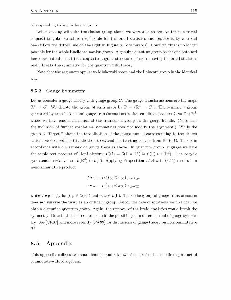
8.A Appendix 115
corresponding to any ordinary group.
When dealing with the translation group alone, we were able to remove the non-trivial
coquasitriangular structure responsible for the braid statistics and replace it by a trivial
one (follow the dotted line on the right in Figure 8.1 downwards). However, this is no longer
possible for the whole Euclidean motion group. A genuine quantum group as the one obtained
here does not admit a trivial coquasitriangular structure. Thus, removing the braid statistics
really breaks the symmetry for the quantum field theory.
Note that the argument applies to Minkowski space and the Poincare group in the identical
way.
8.5.2 Gauge Symmetry
Let us consider a gauge theory with gauge group G. The gauge transformations are the maps
Rd → G. We denote the group of such maps by Γ = Rd → G. The symmetry group
generated by translations and gauge transformations is the semidirect product Ω := Γo Rd,where we have chosen an action of the translation group on the gauge bundle. (Note that
the inclusion of further space-time symmetries does not modify the argument.) While the
group Ω “forgets” about the trivialisation of the gauge bundle corresponding to the chosen
action, we do need the trivialisation to extend the twisting cocycle from Rd to Ω. This is in
accordance with our remark on gauge theories above. In quantum group language we have
the semidirect product of Hopf algebras C(Ω) = C(Γ o Rd) ∼= C(Γ) o C(Rd). The cocycle
χθ extends trivially from C(Rd) to C(Γ). Applying Proposition 2.1.4 with (8.11) results in a
noncommutative product
f • γ = χθ(f (1) ⊗ γ(1)) f (2)γ(2),
γ • ω = χθ(γ(1) ⊗ ω(1)) γ(2)ω(2),
while f • g = fg for f, g ∈ C(Rd) and γ, ω ∈ C(Γ). Thus, the group of gauge transformation
does not survive the twist as an ordinary group. As for the case of rotations we find that we
obtain a genuine quantum group. Again, the removal of the braid statistics would break the
symmetry. Note that this does not exclude the possibility of a different kind of gauge symme-
try. See [CR87] and more recently [SW99] for discussions of gauge theory on noncommutative
Rd.
8.A Appendix
This appendix collects two small lemmas and a known formula for the semidirect product of
commutative Hopf algebras.

116 Quantum Field Theory on Noncommutative Rd
Let H,R be a coquasitriangular Hopf algebra. If R satisfies a certain condition, then for
H-invariant elements the braiding ψ (given by (1.8)) is just the same as the flip map:
Lemma 8.6.1. Let H be a Hopf algebra with coquasitriangular structure R : H ⊗ H → ksatisfying the property R(S a(1)⊗ a(2)) = ε(a). Then for left comodules V and W and v⊗w ∈V ⊗W H-invariant we have ψ(v ⊗ w) = w ⊗ v.
Proof. w(1) ⊗ v(1) ⊗ w(2) ⊗ v(2) = S v(1) ⊗ v(2) ⊗ w ⊗ v(3) due to invariance. Inserting this into
(1.8) gives the desired result.
We note that this property extends to cyclic permutations of invariant elements in multiple
tensor products (just replace V or W by a multiple tensor product).
Given a Hopf algebra H with coquasitriangular structure R, recall from Chapter 2 that
a 2-cocycle χ : H ⊗H → k (Definition 2.1.3) induces a twisted Hopf algebra Hχ with twisted
coquasitriangular structureRχ (Proposition 2.1.4). This gives then rise to a twist of comodule
categories according to Theorem 2.2.2. In this context, we remark that an H-invariant element
of a 2-fold tensor product remains the same under twist if χ satisfies an extra property. This
is the following lemma.
Lemma 8.6.2. In the context of Theorem 2.2.2 let V and W be H-comodules and v ⊗ w ∈V ⊗W be H-invariant. Assume further that χ satisfies χ(a(1)⊗S a(2)) = ε(a). Then σχ
−1(v⊗w) = v ⊗ w.
Proof. First observe that the mentioned property of χ is automatically satisfied by χ−1 as
well. Then use invariance in the form v(1) ⊗ w(1) ⊗ v(2) ⊗ w(2) = v(1) ⊗ S v(2) ⊗ v(3) ⊗ w and
apply σχ−1.
Finally, let us mention that for commutative Hopf algebras C and H with C a left H-
comodule algebra and coalgebra there is a commutative semidirect product Hopf algebra
C o H. It is freely generated by C and H as a commutative algebra. Its coproduct on
elements of H is the given one, while the coproduct on elements of C is modified to
∆o c = c(1)c(2)[1] ⊗ c(2)[2]. (8.11)
Here, brackets denote the coaction to distinguish it from the coproduct. This is the straight-
forward equivalent to a semidirect product of groups in quantum group language. For the
general theory of crossed products of Hopf algebras see [Maj95b].

Chapter 9
φ4-Theory on the Quantum
2-Sphere
The idea that noncommutative geometry might serve as a regulator for quantum field theory
is quite old [Sny47]. One approach that has been quite successful is similar in spirit to lattice
field theory. The infinite dimensional algebra of functions is replaced by a finite dimensional
approximation, so that the path integral is manifestly well-defined and finite. A considerable
advantage over a lattice discretisation is the fact that space-time symmetries are not broken.
See e.g. [Mad92, Mad95, GKP96, Haw99].
The disadvantage as compared to other conventional quantum field theoretic regularisation
methods is the problem of the existence and identification of a “continuum limit”. It would
thus be desirable to find a regularisation that is both continuous and preserves the symmetries.
While such a regularisation is probably non-existent, quantum geometry does seem to offer an
approach that “almost” delivers on this. The idea is to replace symmetry groups by quantum
deformations, so that for a certain value of the deformation parameter the ordinary group
(and theory) is recovered. This was advocated e.g. in [Maj90b].
Braided quantum field theory makes possible a systematic realisation of this idea. This is
the subject of the current chapter. We consider φ4-theory on the quantum 2-sphere [Pod87]
with SUq(2) symmetry. Ordinary φ4-theory in 2 dimensions is super-renormalisable and has
just one basic divergence: the tadpole diagram (Figure 6.7 in Chapter 6). (See e.g. [Zin96]
for a treatment of standard φ4-theory.) We demonstrate that this diagram becomes finite for
q > 1.
We show how the conventional divergence is converted into a divergence in q-parameter
space. The form of the divergence leads us to speculate that conventional divergences irre-
spective of degree could be regularised in this manner. Finally, we consider renormalisation
117

118 φ4-Theory on the Quantum 2-Sphere
of the theory and obtain a nice diagrammatic interpretation of the renormalisation process.
Since SUq(2) is compact we make use of the Peter-Weyl decomposition and have a well-
defined theory in the sense of Section 7.4. Furthermore, like the commutative counterparts,
S2q is a quantum homogeneous space under SUq(2). Thus, we also have the methods of
Section 7.3 at our disposal.
Although we deal with a real scalar field theory we work over the complex numbers. This
is necessary since the standard q-deformations viewed as deformations of complexifications
of compact Lie groups do not restrict to real subalgebras for q 6= 1. However, viewing q-
deformation purely as a regularisation tool we can always restrict to R when considering
physical quantities living at q = 1.
Throughout this chapter, we adopt the convention to denote a Hopf algebra of regular
functions by the name of the respective (quantum) group or space.
9.1 The Decomposition of SUq(2) and S2q
To prepare the ground we need to recall the construction of S2q as a quantum homogeneous
space under SUq(2) and the Peter-Weyl decomposition of the latter [Koo89, MMN+91]. This
will enable us to apply the machinery of the previous chapters.
Recall that SUq(2) is the compact real form of SLq(2). It is cosemisimple and there
is one simple (right) comodule Vl for each integer dimension, conventionally labelled by a
half-integer l such that the dimension is 2l + 1. Thus, the Peter-Weyl decomposition (7.9) is
SUq(2) ∼=⊕
l∈ 12N0
(V ∗l ⊗ Vl).
There is a Hopf ∗-algebra surjection π : SUq(2) → U(1) corresponding to the diagonal
inclusion in the commutative case. This defines the quantum 2-sphere S2q as the right ho-
mogeneous ∗-space U(1)SUq(2). Under the coaction of U(1) induced by π the comodules Vl
decompose into inequivalent one-dimensional comodules. Those are classified by integers i
such that the coaction takes the form v 7→ v⊗gi. This determines up to normalisation a basis
v(l)n for Vl, where n are half-integers such that the coaction of U(1) is v
(l)n 7→ v
(l)n ⊗ g−2n. It
turns out that the indices n take the values −l,−l+1, . . . , l. In particular, we find that VU(1)l
is one-dimensional if l is integer and zero-dimensional otherwise. Thus, (7.10) simplifies to
S2q∼=⊕
l∈N0
Vl
as right SUq(2)-comodules. We write the induced (normalisation independent) basis vectors
of SUq(2) as t(l)i j = (f
(l)i ⊗ id) β(e
(l)j ) where f
(l)n is dual to e
(l)n and β : Vl → Vl ⊗ SUq(2)

9.1 The Decomposition of SUq(2) and S2q 119
is the coaction of SUq(2) on Vl. As a subalgebra S2q has the basis t(l)0 i. The bi-invariant
subalgebra S2qU(1)
= U(1)SUq(2)U(1) has the basis t(l)0 0.Note that by construction
ε(t(l)mn
)= δm,n and ∆ t(l)mn =
∑
k
t(l)mk ⊗ t
(l)k n.
The antipode and ∗-structure of SUq(2) in this basis are
S t(l)mn = (−q)m−nt(l)−n−m,(t(l)mn
)∗= S t(l)nm = (−q)n−mt(l)−m−n,
as can be verified by direct calculation from the formulas in [KS97, 4.2.4]. The normalised
invariant integral (Haar functional) is simply∫t(l)i j = δl,0. We also need its value on the
product of two basis elements
∫t(l)mnt
(l′)m′ n′ =
(−1)m−nqm+n
[2l + 1]′qδl,l′δm+m′,0δn+n′,0. (9.1)
This can be easily worked out considering the equation ε(a) =∫a(1) S a(2) and using the
invariance of the integral in the form b(1)
∫ab(2) = S a(1)
∫a(2)b and S b(2)
∫ab(1) = a(2)
∫a(1)b
on basis elements. We need q-integers for q ∈ C∗ defined as
[n]′q :=n−1∑
k=0
qn−2k−1 =qn − q−nq − q−1
.
(The second expression is only defined for q2 6= 1).
Denoting a dual basis of t(l)mn by t(l)mn, we observe that SUq(2)∗ becomes an object in
MSUq(2) with evaluation ev : SUq(2)⊗ SUq(2)∗ → C and coevaluation coev : C→ SUq(2)∗ ⊗SUq(2) by the coaction t
(l)mn 7→
∑k t
(l)mk ⊗ S−1 t
(l)nk.
In the commutative case q = 1, the basis t(l)mn becomes the usual basis of regular
functions (i.e., matrix elements of representations) on SU(2) (see e.g. [VK91, Chapter 6] to
whose conventions we conform in this case). The restriction to t(l)0n recovers nothing but (a
version of) the spherical harmonics on S2. In particular, we notice that the zonal spherical
functions can be expressed in terms of Legendre polynomials t(l)0 0(φ, θ, ψ) = Pl(cos θ), where
φ, θ, ψ are the Euler angles on SU(2) (see [VK91, Chapter 6]). From the orthogonality
relation of the Legendre polynomials, the fact that their only common value is at Pl(1) = 1,
and considering that θ = 0 denotes a pole of SU(2), we find that the delta function at the
identity of SU(2) restricted to S2 can be represented as
δ0(φ, θ) =∑
l
(2l + 1)Pl(cos θ) =∑
l
(2l + 1) t(l)0 0(φ, θ). (9.2)

120 φ4-Theory on the Quantum 2-Sphere
For calculations we need the functionals u and v defined for a coquasitriangular structure
R as (see e.g. [Maj95b])
u(a) := R(a(2) ⊗ S a(1)), v(a) := R(a(1) ⊗ S a(2)). (9.3)
For SUq(2) in our basis they are
u(t(l)mn) = δm,n q−2l(l+1)+2m, v(t(l)mn) = δm,n q
−2l(l+1)−2m. (9.4)
We also note that property (7.8) is satisfied, i.e.,
R(t(l)0 0 ⊗ t
(l)i j
)= δi,j = R
(t(l)i j ⊗ t
(l)0 0
). (9.5)
See Appendix 9.A for a derivation of (9.4) and (9.5).
9.2 The Free Propagator
In ordinary quantum field theory the free propagator is defined by the free action. For a
Euclidean massive real scalar field theory on a manifold M it takes the form
S0(φ) =1
2
∫
Mdxφ(x)(m2 −∆M )φ(x),
where ∆M is the Laplace operator on M and m is the mass of the field. Define L := m2−∆M .
Applying equation (6.13) we obtain in the more abstract notation of Section 6.1.1
γ =
(id⊗
∫
M
) (id⊗·) (coev⊗L), (9.6)
which we take as the defining equation for γ.
In the noncommutative case q 6= 1 we still have an integral on our “manifold” M = S2q . We
further need an analogue of the Laplace operator. We note that by the duality of SUq(2) with
the quantum enveloping algebra Uq(sl2), a central element of the latter defines an invariant
operator on SUq(2)-comodules. A natural choice is the quantum Casimir element which we
define as
Cq = EF +(K − 1)q−1 + (K−1 − 1)q
(q − q−1)2.
Here K, K−1, E, and F are the generators of Uq(sl2) (see Appendix 9.A). Cq differs from
quantum Casimir elements considered elsewhere (see e.g. [MMN+91] or [KS97]) only by a
q-multiple of the identity. The eigenvalue of Cq on Vl is [l]′q[l + 1]′q so that we get exactly the
(negative of the) usual Laplace operator for q = 1. Including a mass term we set
L = Cq +m2.

9.3 Interactions 121
Thus, the eigenvalue of L on Vl is
Ll = [l]′q[l + 1]′q +m2.
We determine γ−1 according to (9.6). Using (9.1) we find
γ(t(l)0 i
)=∑
m,j
t(m)0 j
∫t(m)0 j L
(t(l)0 i
)= [2l + 1]′q
−1Ll (−q)−i t(l)0−i.
Inverting we obtain
γ−1(t(l)0 i
)= [2l + 1]′q L−1
l (−q)−i t(l)0−i.
Now, we are ready to determine the free propagator according to Corollary 6.2.1.
Z2 =∑
l,k
(id⊗γ−1) ψ(t(l)0 k ⊗ t
(l)0 k
)
=∑
l,i,j,k
t(l)0 i ⊗ γ−1
(t(l)0 j
)R(
S−1 t(l)k j ⊗ t
(l)i k
)
=∑
l,i,j
t(l)0 i ⊗ γ−1
(t(l)0 j
)u(t(l)i j
)
=∑
l,i
[2l + 1]′q L−1l q−2l(l+1) (−q)i t(l)0 i ⊗ t
(l)0−i.
Using invariant reduction (Proposition 7.3.2) we find
Z2=∑
l
[2l + 1]′q L−1l q−2l(l+1) t
(l)0 0 (9.7)
to be the reduced form of the propagator as an element of S2qU(1)
. In the commutative case
(q = 1) we can rewrite (9.7) as
Z2 |q=1 = (m2 −∆)−1δ0
by comparison with (9.2). This is the familiar expression from ordinary quantum field theory.
9.3 Interactions
We proceed to evaluate the order 1 contribution of the φ4-interaction to the 2-point function.
The corresponding diagrams are depicted in Figure 6.6 (see Section 6.2.2). Since the property
(7.8) holds in SUq(2) the diagrams simplify to those of Figure 7.6 (see Section 7.3.2). The
disconnected loop comes out as
δloop := =∑
l
[2l + 1]′q[l]′q[l + 1]′q +m2
q−2l(l+1). (9.8)

122 φ4-Theory on the Quantum 2-Sphere
(Just apply the counit to (9.7).) The connected diagram in the right-hand summand of
Figure 7.6 is (in reduced form)
=
(id⊗ ε⊗
∫ ) (id2⊗·) (id⊗Z2⊗ id) Z2
=∑
l,m,i,j
αlαm t(l)0 i ε
(t(m)0 j
)∫S t
(m)j 0 S t
(l)i 0
=∑
l
α2l [2l + 1]′q
−1t(l)0 0,
with αl := [2l + 1]′q L−1l q−2l(l+1). We have used Z2 as reconstructed from its reduced form
(9.7), the property∫S =
∫of the integral, and (9.1). The connected diagram in the left-
hand summand of Figure 7.6 is (in reduced form)
=
(id⊗ ε⊗
∫ ) (id2⊗·) (id⊗ψ−1 ⊗ id) (Z2⊗Z2)
=∑
l,m,i,j,k,n
αlαm t(l)0 i ε
(t(m)0 k
)∫S t
(l)n 0 S t
(m)j 0 R−1
(t(m)k j ⊗ S t
(l)i n
)
=∑
l,m,i,j,n
αlαm t(l)0 i
∫t(m)j 0 t
(l)n 0R
(t(m)0 j ⊗ t
(l)i n
)
=∑
l,m,i,j,k
αlαm t(l)0 i
∫t(m)k 0 t
(l)i 0 R
(t(m)0 j ⊗ S t
(m)j k
)
=∑
l,m,i,k
αlαm t(l)0 i
∫t(m)k 0 t
(l)i 0 v
(t(m)0 k
)
=∑
l
α2l [2l + 1]′q
−1q−2l(l+1) t
(l)0 0.
We have also used the invariance of the integral in the form (∫ab(2))b(1) = (
∫a(2)b) S a(1) in
the third equality. Thus, the (reduced) 2-point function up to order 1 comes out as
Z2
int =∑
l
[2l + 1]′q L−1l q−2l(l+1) t
(l)0 0
(1− 6λ δloop L−1
l q−2l(l+1)(1 + q−2l(l+1)) +O(λ2)).
(9.9)
In the commutative case (q = 1), we know that the order 1 contribution (given by the tadpole
diagram in Figure 6.7) is divergent. We can easily see where this divergence comes from. The
loop contribution (9.8)
δloop|q=1 =∑
l
2l + 1
l(l + 1) +m2(9.10)

9.4 Renormalisation 123
is infinite. However, at q > 1 it becomes finite! We are truly able the regularise the tadpole
diagram. Let us identify the divergence in q-space. For q > 1 we can find both an upper and
a lower bound for (9.8) of the form
const +
∫ ∞
1dl
2
lq−2l2 ,
where const does not depend on q (but may depend on m2). Setting q = e2h2with h > 0 we
find
δloop|q>1 =1
h+O(1).
The conventional divergence of (9.10) is only logarithmic in l. What would happen with
higher divergences? It seems natural to assume that they would give rise to terms like
∑
l
[l]′qnq−2l(l+1).
But this converges in the domain q > 1 for any n. We can even apply the very same discussion
of the divergence in q-space as above. The nature of the divergence in q-space does not seem
to be affected by the degree of the ordinary (commutative) divergence at all. This suggests
that q-regularization in our framework is powerful indeed. Compare this, e.g., to dimensional
regularization which can only handle logarithmic divergences.
Reviewing our calculations of Z2 and Z2int we find that the crucial factor of q−2l(l+1) is
caused by the braiding. Thus, the braiding and not the mere noncommutativity appears to
be essential for the regularisation.
9.4 Renormalisation
Ordinarily, φ4-theory in dimension 2 is super-renormalisable. The only basic divergent di-
agram is the tadpole (Figure 6.7). Thus, if in a given diagram we separate out all loops
from “tadpole vertices” according to Figures 7.4 and 7.5 (as we did in the last section for the
tadpole), the remaining diagram is finite at q = 1. The “stripped” vertices have just become
φ2-vertices. Notice however, that from a rigorous point of view this can only be done if the
whole diagram is finite. While we have seen that the tadpole diagram alone becomes finite for
q > 1, it is conceivable that certain diagrams that converge at q = 1 would diverge at q > 1.
This might be due to the introduction of factors like q2l(l+1) into summations over l. The
expression (9.9) suggests, however, that this does not happen, but rather that all q-factors
introduced in summations have negative exponent. We shall assume this in the following.

124 φ4-Theory on the Quantum 2-Sphere
Let us now see what renormalisation looks like in our framework. To renormalise the
coupling we set
λ′ := λ δloop
at q > 1 and fix λ′ as our new coupling. Then, given any diagram we perform the stripping
of tadpole loops as described above and the separated loops cancel with δ−1loop in λ′. As q goes
to 1 those loops are just φ2 vertices. However, in this limit, any other vertex vanishes due to
a factor of δ−1loop. Thus, we remain with only φ2-vertices corresponding to an additional mass
term. The effective shift in mass is
m2 → m2 + 12λ′.
What one usually does in φ4-theory is to renormalise the mass to cancel the divergence.
Thus, instead of redefining λ we set
m2 := m2 − 12λ δloop.
to be the new mass. Of course this equation must not be understood literally in our framework
since we cannot write the free and the interacting part of the action together. Instead, we
introduce (at q > 1) a φ2 vertex with a factor of −6λ δloop in front. Writing all diagrams of
a given order in λ, all tadpoles are canceled in the limit q → 1, and only finite non-tadpole
vertices remain.
9.A Appendix: Coquasitriangular Structure of SUq(2)
In this appendix we provide the required formulas for the coquasitriangular structure of
SUq(2) in our Peter-Weyl basis. We use the context of Section 9.1. Definitions and results
that are just stated are standard and can be found e.g. in [Maj95b] or [KS97].
The Hopf algebra Uq(sl2) is defined over C for q ∈ C∗ and q2 6= 1 with generators
E,F,K,K−1 and relations
KEK−1 = q2E, KFK−1 = q−2F,
KK−1 = K−1K = 1, [E,F ] =K −K−1
q − q−1,
∆(E) = E ⊗K + 1⊗ E, ∆(F ) = F ⊗ 1 +K−1 ⊗ F,∆(K) = K ⊗K, ε(K) = 1, ε(E) = ε(F ) = 0,
S(K) = K−1, S(E) = −EK−1, S(F ) = −KF.

9.A Appendix: Coquasitriangular Structure of SUq(2) 125
Uq(sl2) and SUq(2) are non-degenerately paired. Thus, actions of Uq(sl2) and coactions
of SUq(2) on finite dimensional vector spaces are dual to each other. In particular, the simple
comodule Vl of SUq(2) is a simple module of Uq(sl2). By the representation theory of Uq(sl2)
it has a basis wi, i = −l,−l + 1, . . . , l such that
K . wm = q2mwm, E . wm = ([l −m]′q[l +m+ 1]′q)1/2wm+1
F . wm = ([l +m]′q[l −m+ 1]′q)1/2wm−1.
(9.11)
Uq(sl2) has an h-adic version Uh(sl2) defined over C[[h]] correspondingly with q = eh and
an additional generator H so that qH = K. It has the quasitriangular structure
R = q(H⊗H)/2∞∑
n=0
qn(n+1)/2(1− q−2)n
[n]′q!En ⊗ Fn. (9.12)
The elements (define R(1) ⊗R(2) = R)
u′ = (SR(2))R(1), v′ = R(1) SR(2) (9.13)
act on Vl as [Maj95b, Proposition 3.2.7]
u′ . wm = q−2l(l+1)+2mwm, v′ . wm = q−2l(l+1)−2mwm. (9.14)
The coquasitriangular structure R of SUq(2) is given by the duality with Uq(sl2) from the
quasitriangular structure R of Uh(sl2). Using
u(a(1))a(2) = S2 a(1)u(a(2)) and v(a(1)) S2 a(2) = a(1)v(a(2))
we find
u(t(l)mn
)= δm,n q
2(m−k)u(t(l)k k
), v
(t(l)mn
)= δm,n q
2(k−m)v(t(l)k k
). (9.15)
Since the definitions (9.3) and (9.13) are dual to each other we can use
g . vn =∑
m
vm〈g, t(l)mn〉, g ∈ Uq(sl2)
to compare (9.14) with (9.15). We find (9.4) and infer that wi is (a multiple of) vi. With the
latter, the pairing between Uq(sl2) and SUq(2) comes out from (9.11) as
〈K, t(l)mn〉 = δm,n q2n, 〈E, t(l)mn〉 = δm,n+1([l − n]′q[l + n+ 1]′q)
1/2,
〈F, t(l)mn〉 = δm,n−1([l + n]′q[l − n+ 1]′q)1/2.
Note also 〈H, t(l)mn〉 = δm,n2n in the h-adic version. With this pairing and (9.12) we easily
verify the property (9.5).

Bibliography
[Abe80] E. Abe, Hopf algebras, Cambridge University Press, Cambridge, 1980.
[Bar54] V. Bargmann, On unitary ray representations of continuous groups, Ann. of Math.
59 (1954), 1–46.
[BFF+78] F. Bayen, M. Flato, C. Fronsdal, A. Lichnerowitz, and D. Sternheimer, Deforma-
tion Theory and Quantization. I,II, Ann. Phys. 111 (1978), 61–151.
[BM93] T. Brzezinski and S. Majid, Quantum Group Gauge Theory on Quantum Spaces,
Commun. Math. Phys. 157 (1993), 591–638.
[Brz93] T. Brzezinski, Remarks on Bicovariant Differential Calculi and Exterior Hopf
Algebras, Lett. Math. Phys. 27 (1993), 287–300.
[BS98] P. Baumann and F. Schmitt, Classification of Bicovariant Differential Calculi on
Quantum Groups (a representation-theoretic approach), Commun. Math. Phys.
194 (1998), 71–86.
[CDS98] A. Connes, M. R. Douglas, and A. Schwarz, Noncommutative geometry and Ma-
trix theory, J. High Energy Phys. 9802 (1998), 003.
[CL90] A. Connes and J. Lott, Particle models and noncommutative geometry, Recent
advances in field theory (Annecy-le-Vieux, 1990), Nucl. Phys. B Proc. Suppl.,
vol. 18B, 1990, pp. 29–47.
[Con80] A. Connes, C∗-algebres et geometrie differentielle, C. R. Acad. Sci. Paris A 290
(1980), 599–604.
[Con85] A. Connes, Noncommutative differential geometry, Inst. Hautes Etudes Sci. Publ.
Math. (1985), no. 62, 257–360.
[Con94] A. Connes, Noncommutative Geometry, Academic Press, London, 1994.
126

BIBLIOGRAPHY 127
[CP94] V. Chari and A. Pressley, A guide to Quantum Groups, Cambridge University
Press, Cambridge, 1994.
[CR87] A. Connes and M. A. Rieffel, Yang-Mills for non-commutative two-tori, Operator
Algebras and Mathematical Physics (Iowa City, 1985), Contemp. Math., no. 62,
Amer. Math. Soc., Providence, R.I., 1987, pp. 237–266.
[CR00] I. Chepelev and R. Roiban, Renormalisation of quantum field theories on non-
commutative Rd, I. Scalars, J. High Energy Phys. 0005 (2000), 037.
[CSM95] R. Carter, G. Segal, and I. MacDonald, Lectures on Lie Groups and Lie Algebras,
Cambridge University Press, Cambridge, 1995.
[CSSW90] U. Carow-Watamura, M. Schlieker, M. Scholl, and S. Watamura, Tensor rep-
resentation of the quantum group SLq(2,C) and quantum Minkowski space, Z.
Phys. C 48 (1990), 159–165.
[CSWW91] U. Carow-Watamura, M. Schlieker, S. Watamura, and W. Weich, Bicovariant
Differential Calculus on Quantum Groups SUq(N) and SOq(N), Commun. Math.
Phys. 142 (1991), 605–641.
[DFR95] S. Doplicher, K. Fredenhagen, and J. E. Roberts, The Quantum Structure of
Spacetime at the Planck Scale and Quantum Fields, Commun. Math. Phys. 172
(1995), 187–220.
[Dri83a] V. G. Drinfeld, Hamiltonian structures on Lie groups, Lie bialgebras and the
geometric meaning of the classical Yang-Baxter equations, Soviet Math. Dokl. 27
(1983), 68–71.
[Dri83b] V. G. Drinfeld, On constant, quasiclassical solutions of the Yang-Baxter Quantum
Equation, Soviet Math. Dokl. 28 (1983), 531–535.
[Dri85] V. G. Drinfeld, Hopf algebras and the quantum Yang-Baxter equation, Soviet
Math. Dokl. 32 (1985), 254–258.
[Dri87] V. G. Drinfeld, Quantum Groups, Proceedings of the ICM 1986 (A. Gleason, ed.),
AMS, Rhode Island, 1987, pp. 798–820.
[Dri90] V. G. Drinfeld, Quasi-Hopf Algebras, Leningrad Math. J. 1 (1990), 1419–1457.
[FG90] J. Frohlich and F. Gabbiani, Braid Statistics in Local Quantum Theory, Rev.
Math. Phys. 2 (1990), 251–353.

128 BIBLIOGRAPHY
[Fie39] M. Fierz, Uber die relativistische Theorie kraftefreier Teilchen mit beliebigem
Spin, Helv. Phys. Acta 12 (1939), 3–37.
[Fil96] T. Filk, Divergencies in a field theory on quantum space, Phys. Lett. B 376
(1996), 53–58.
[FRS89] K. Fredenhagen, K. H. Rehren, and B. Schroer, Superselection sectors with braid
group statistics and exchange algebras. I. General theory, Commun. Math. Phys.
125 (1989), 201–226.
[GH99] O. W. Greenberg and R. C. Hilborn, Quon Statistics for Composite Systems and
a Limit on the Violation of the Pauli Principle for Nucleons and Quarks, Phys.
Rev. Lett. 83 (1999), 4460–4463.
[GKM96] C. Gonera, P. Kosinski, and P. Maslanka, Differential Calculi on Quantum
Minkowski Space, J. Math. Phys. 37 (1996), 5820–5827.
[GKP96] H. Grosse, C. Klimcik, and P. Presnajder, On Finite 4D Quantum Field Theory
in Non-Commutative Geometry, Commun. Math. Phys. 180 (1996), 429–438.
[Gre91] O. W. Greenberg, Particles with small violations of Fermi or Bose statistics,
Phys. Rev. D 43 (1991), 4111–4119.
[Haw99] E. Hawkins, Noncommutative Regularization for the Practical Man, Preprint hep-
th/9908052, 1999.
[HS97] I. Heckenberger and K. Schmudgen, Bicovariant Differential Calculi on SLq(N)
and Spq(N), Czech. J. Phys. 47 (1997), 1145–1151.
[HW98] P.-M. Ho and Y.-S. Wu, Noncommutative gauge theories in matrix theory, Phys.
Rev. D 58 (1998), 066003.
[Jim85] M. Jimbo, A q-difference analogue of U(g) and the Yang-Baxter equation, Lett.
Math. Phys. 10 (1985), 63–69.
[JS86] A. Joyal and R. Street, Braided monoidal categories, Macquarie Math. Reports
no 86081, 1986.
[Jur91] B. Jurco, Differential Calculus on Quantized Simple Lie Groups, Lett. Math.
Phys. 22 (1991), 177–186.
[Kem97] A. Kempf, On quantum field theory with nonzero minimal uncertainties in posi-
tions and momenta, J. Math. Phys. 38 (1997), 1347–1372.

BIBLIOGRAPHY 129
[KM94] A. Kempf and S. Majid, Algebraic q-integration and Fourier theory on quantum
and braided spaces, J. Math. Phys. 35 (1994), 6802–6837.
[Koo89] T. H. Koornwinder, Representations of the twisted SU(2) quantum group and
some q-hypergeometric orthogonal polynomials, Nederl. Akad. Wetensch. Proc.
Ser. A 92 (1989), 97–117.
[KS97] A. Klimyk and K. Schmudgen, Quantum Groups and Their Representations,
Springer Verlag, Berlin, 1997.
[LM77] J. M. Leinaas and J. Myrheim, On the Theory of Identical Particles, Nuovo
Cimento B 37 (1977), 1–23.
[LNR92] J. Lukierski, A. Nowicki, and H. Ruegg, New quantum Poincare algebra and κ-
deformed field theory, Phys. Lett. B 293 (1992), 344–352.
[Mac98] S. Mac Lane, Categories for the Working Mathematician, 2nd ed., Springer, New
York, 1998.
[Mad92] J. Madore, Fuzzy Physics, Ann. Phys. 219 (1992), 187–198.
[Mad95] J. Madore, An Introduction to Noncommutative Differential Geometry and its
Physical Applications, Cambridge University Press, Cambridge, 1995.
[Maj88] S. Majid, Hopf algebras for physics at the Planck scale, Class. Quantum Grav. 5
(1988), 1587–1606.
[Maj90a] S. Majid, Matched pairs of Lie groups associated to solutions of the Yang-Baxter
equations, Pacific J. Math. 141 (1990), 311–332.
[Maj90b] S. Majid, On q-Regularization, Int. J. Mod. Phys. A 5 (1990), 4689–4696.
[Maj91] S. Majid, Hopf-von Neumann algebra bicrossproducts, Kac algebra bicrossprod-
ucts, and the classical Yang-Baxter equations, J. Funct. Anal. 95 (1991), 291–319.
[Maj93a] S. Majid, Anyonic Quantum Groups, Spinors, Twistors, Clifford Algebras and
Quantum Deformations (Z. Oziewicz, B. Janewicz, and A. Borowiec, eds.), Fund.
Theories Phys., vol. 52, Kluwer Academic, Dordrecht, 1993, pp. 327–336.
[Maj93b] S. Majid, Free braided differential calculus, braided binomial theorem, and the
braided exponential map, J. Math. Phys. 34 (1993), 4843–4856.
[Maj94] S. Majid, q-Euclidean space and quantum Wick rotation by twisting, J. Math.
Phys. 35 (1994), 5025–5034.

130 BIBLIOGRAPHY
[Maj95a] S. Majid, Duality principle and braided geometry, Strings and Symmetries (Is-
tanbul, 1994), Lecture Notes in Phys., vol. 447, Springer Verlag, Berlin, 1995,
pp. 125–144.
[Maj95b] S. Majid, Foundations of Quantum Group Theory, Cambridge University Press,
Cambridge, 1995.
[Maj98] S. Majid, Classification of Bicovariant Differential Calculi, J. Geom. Phys. 25
(1998), 119–140.
[MMN+91] T. Masuda, K. Mimachi, Y. Nakagami, M. Noumi, and K. Ueno, Representations
of the Quantum Group SUq(2) and the Little q-Jacobi Polynomials, J. Funct.
Anal. 99 (1991), 357–386.
[MO99] S. Majid and R. Oeckl, Twisting of Quantum Differentials and the Planck Scale
Hopf Algebra, Commun. Math. Phys. 205 (1999), 617–655.
[Moy49] J. E. Moyal, Quantum mechanics as a statistical theory, Proc. Cambridge Philos.
Soc. 45 (1949), 99–124.
[MR94] S. Majid and H. Ruegg, Bicrossproduct structure of κ-Poincare group and non-
commutative geometry, Phys. Lett. B 334 (1994), 348–354.
[MS96] S. Major and L. Smolin, Quantum deformation of quantum gravity, Nucl. Phys.
B 473 (1996), 267–290.
[MVS00] S. Minwalla, M. Van Raamsdonk, and N. Seiberg, Noncommutative Perturbative
Dynamics, J. High Energy Phys. 0002 (2000), 020.
[Oec99a] R. Oeckl, Braided Quantum Field Theory, Preprint hep-th/9906225, 1999.
[Oec99b] R. Oeckl, Classification of differential calculi on Uq(b+), classical limits, and
duality, J. Math. Phys. 40 (1999), 3588–3603.
[Oec00a] R. Oeckl, The Quantum Geometry of Spin and Statistics, Preprint hep-
th/0008072, 2000.
[Oec00b] R. Oeckl, Untwisting noncommutative Rd and the equivalence of quantum field
theories, Nucl. Phys. B 581 (2000), 559–574.
[OSWZ92] O. Ogievetsky, W. B. Schmidke, J. Wess, and B. Zumino, q-Deformed Poincare
algebra, Commun. Math. Phys. 150 (1992), 495–518.

BIBLIOGRAPHY 131
[Pau40] W. Pauli, The Connection Between Spin and Statistics, Phys. Rev. 58 (1940),
716–722.
[Pod87] P. Podles, Quantum Spheres, Lett. Math. Phys. 14 (1987), 193–202.
[PW90] P. Podles and S. L. Woronowicz, Quantum deformation of Lorentz group, Com-
mun. Math. Phys. 130 (1990), 381–431.
[Rad85] D. E. Radford, The structure of Hopf algebras with a projection, J. Algebra 92
(1985), 322–347.
[RTF90] N. Yu. Reshetikhin, L. A. Takhtadzhyan, and L. D. Faddeev, Quantization of Lie
groups and Lie algebras, Leningrad Math. J. 1 (1990), 193–225.
[Sch94] P. Schauenburg, Hopf Modules and Yetter-Drinfeld Modules, J. Algebra 169
(1994), 874–890.
[Sny47] H. S. Snyder, Quantized Space-Time, Phys. Rev. 71 (1947), 38–41.
[SS95] K. Schmudgen and A. Schuler, Classification of Bicovariant Differential Calculi
on Quantum Groups, Commun. Math. Phys. 170 (1995), 315–335.
[SW99] N. Seiberg and E. Witten, String theory and noncommutative geometry, J. High
Energy Phys. 9909 (1999), 032.
[Swe69] M. E. Sweedler, Hopf Algebras, W. A. Benjamin, New York, 1969.
[VK91] N. Ja. Vilenkin and A. U. Klimyk, Representation of Lie Groups and Special
Functions, vol. 1, Kluwer Academic, Dordrecht, 1991.
[VV99] S. Vaes and A. Van Daele, Hopf C∗-algebras, Preprint math.OA/9907030, 1999.
[Wat00] P. Watts, Noncommutative string theory, the R-matrix, and Hopf algebras, Phys.
Lett. B 474 (2000), 295–302.
[Wey31] H. Weyl, The Theory of Groups and Quantum Mechanics, Methuen, London,
1931.
[Wil82] F. Wilczek, Quantum Mechanics of Fractional-Spin Particles, Phys. Rev. Lett.
49 (1982), 957–959.
[Wil90] F. Wilczek, Fractional Statistics and Anyon Superconductivity, World Scientific,
Singapore, 1990.

132 BIBLIOGRAPHY
[Wor87] S. L. Woronowicz, Compact Matrix Pseudogroups, Commun. Math. Phys. 111
(1987), 613–665.
[Wor89] S. L. Woronowicz, Differential Calculus on Compact Matrix Pseudogroups (Quan-
tum Groups), Commun. Math. Phys. 122 (1989), 125–170.
[Wu84] Y.-S. Wu, General Theory of Quantum Statistics in Two Dimensions, Phys. Rev.
Lett. 52 (1984), 2103–2106.
[Yet90] D. N. Yetter, Quantum groups and representations of monoidal categories, Math.
Proc. Camb. Phil. Soc. 108 (1990), 261–290.
[Zin96] J. Zinn-Justin, Quantum Field Theory and Critical Phenomena, 3rd ed., Oxford
University Press, Oxford, 1996.


![HOLOGRAPHY, QUANTUM GEOMETRY, AND QUANTUM INFORMATION THEORY · The emerging fields of quantum computation [22], quantum communication and quantum cryptography [23], quantum dense](https://static.fdocuments.net/doc/165x107/5ec76f6b603b2e345706bd5a/holography-quantum-geometry-and-quantum-information-theory-the-emerging-fields.jpg)


