Quantum Fields on CausalSets - arXivAbstract Causal set theory provides a model of discrete...
172
arXiv:1010.5514v1 [hep-th] 26 Oct 2010 Quantum Fields on Causal Sets by Steven Paul Johnston MSci Mathematics, Imperial College London, 2006 Submitted to the Department of Physics at Imperial College London in partial fulfillment of the requirements for the degree of Doctor of Philosophy (Theoretical Physics, University of London) and Diploma of Imperial College London September 2010 1
Transcript of Quantum Fields on CausalSets - arXivAbstract Causal set theory provides a model of discrete...

arX
iv:1
010.
5514
v1 [
hep-
th]
26
Oct
201
0
Quantum Fields on Causal Sets
by
Steven Paul Johnston
MSci Mathematics, Imperial College London, 2006
Submitted to the Department of Physics at Imperial College London in partial
fulfillment of the requirements for the degree of
Doctor of Philosophy
(Theoretical Physics, University of London)
and
Diploma of Imperial College London
September 2010
1

Declaration
I declare that this work is entirely my own, except where otherwise stated. Parts
of Chapter 3 appear in Johnston (2008a, 2009b). Parts of Chapter 4 appear in
Johnston (2009a).
Signed: September 2010.
Acknowledgements
It is a pleasure to thank the numerous people that have helped me over the
last four years, during which time it has been a privilege to work on causal set
theory. I thank my supervisor, Fay Dowker, for her support and advice. Her
knowledgeable and balanced guidance has been invaluable.
I also thank Rafael Sorkin for repeated helpful exchanges, David Rideout for
help with simulations, Joe Henson and Graham Brightwell for their willingness
to discuss my work. Also Sumati Surya for her friendly hospitality and interest.
I am grateful to Johan Noldus who provided a crucial insight for the work in
Chapter 4. I am also grateful to Noel Hustler and Bernhard Schmitzer for their
interest and discussions.
I thank the theoretical physics group at Imperial College for their help over
the past four years. Amongst my fellow students I thank Leron Borsten for his
encouragement and friendship, Dionigi Benincasa for being a good travelling
companion, Duminda Dahanayake, Lydia Philpott, Will Rubens, Jamie Vicary,
Ben Withers and James Yearsley for their friendship and varied perspectives on
current physics.
Of course I thank my friends and family, in particular my parents for their
support. Special mention belongs to my wife Ashley—I thank her for her love,
constant support and encouragement.
2

Abstract
Causal set theory provides a model of discrete spacetime in which spacetime
events are represented by elements of a causal set—a locally finite, partially
ordered set in which the partial order represents the causal relationships between
events. The work presented here describes a model for matter on a causal
set, specifically a theory of quantum scalar fields on a causal set spacetime
background.
The work starts with a discrete path integral model for particles on a causal
set. Here quantum mechanical amplitudes are assigned to trajectories within
the causal set. By summing these over all trajectories between two spacetime
events we obtain a causal set particle propagator. With a suitable choice of
amplitudes this is shown to agree (in an appropriate sense) with the retarded
propagator for the Klein-Gordon equation in Minkowski spacetime.
This causal set propagator is then used to define a causal set analogue of
the Pauli-Jordan function that appears in continuum quantum field theories. A
quantum scalar field is then modelled by an algebra of operators which satisfy
three simple conditions (including a bosonic commutation rule). Defining time-
ordering through a linear extension of the causal set these field operators are
used to define a causal set Feynman propagator. Evidence is presented which
shows agreement (in a suitable sense) between the causal set Feynman propaga-
tor and the continuum Feynman propagator for the Klein-Gordon equation in
Minkowski spacetime. The Feynman propagator is obtained using the eigende-
composition of the Pauli-Jordan function, a method which can also be applied
in continuum-based theories.
The free field theory is extended to include interacting scalar fields. This
leads to a suggestion for a non-perturbative S-matrix on a causal set. Models
for continuum-based phenomenology and spin-half particles on a causal set are
also presented.
3

Contents
Abstract 3
1 Introduction 81.1 Quantum gravity . . . . . . . . . . . . . . . . . . . . . . . . . . . . . . 81.2 Spacetime and causality . . . . . . . . . . . . . . . . . . . . . . . . . . 9
1.2.1 Spacetime in general relativity . . . . . . . . . . . . . . . . . . 101.2.2 Causal structure . . . . . . . . . . . . . . . . . . . . . . . . . . 11
1.3 Discreteness . . . . . . . . . . . . . . . . . . . . . . . . . . . . . . . . . 131.3.1 The Planck scale . . . . . . . . . . . . . . . . . . . . . . . . . . 131.3.2 Technical problems with the continuum . . . . . . . . . . . . . 141.3.3 Conceptual problems with the continuum . . . . . . . . . . . . 15
2 Causal Sets 172.1 Partial orders . . . . . . . . . . . . . . . . . . . . . . . . . . . . . . . . 172.2 What is a causal set? . . . . . . . . . . . . . . . . . . . . . . . . . . . . 18
2.2.1 Similar approaches . . . . . . . . . . . . . . . . . . . . . . . . . 192.3 Correspondence with the continuum . . . . . . . . . . . . . . . . . . . 20
2.3.1 Embeddings . . . . . . . . . . . . . . . . . . . . . . . . . . . . . 202.3.2 Sprinklings . . . . . . . . . . . . . . . . . . . . . . . . . . . . . 212.3.3 Dynamics . . . . . . . . . . . . . . . . . . . . . . . . . . . . . . 23
2.4 Definitions . . . . . . . . . . . . . . . . . . . . . . . . . . . . . . . . . . 242.5 Representing causal sets . . . . . . . . . . . . . . . . . . . . . . . . . . 25
2.5.1 Hasse diagrams and directed graphs . . . . . . . . . . . . . . . 262.5.2 Adjacency matrices . . . . . . . . . . . . . . . . . . . . . . . . . 27
3 Path Integrals 313.1 Particle models . . . . . . . . . . . . . . . . . . . . . . . . . . . . . . . 31
3.1.1 Swerves . . . . . . . . . . . . . . . . . . . . . . . . . . . . . . . 323.1.2 Hemion classical model . . . . . . . . . . . . . . . . . . . . . . 333.1.3 Discrete path integrals . . . . . . . . . . . . . . . . . . . . . . . 33
3.2 Causal set path integrals . . . . . . . . . . . . . . . . . . . . . . . . . . 343.2.1 The models . . . . . . . . . . . . . . . . . . . . . . . . . . . . . 35
3.3 Propagators in the continuum . . . . . . . . . . . . . . . . . . . . . . . 373.4 Dimensional analysis . . . . . . . . . . . . . . . . . . . . . . . . . . . . 393.5 Expected values . . . . . . . . . . . . . . . . . . . . . . . . . . . . . . . 39
3.5.1 Summing over chains . . . . . . . . . . . . . . . . . . . . . . . . 403.5.2 Summing over paths . . . . . . . . . . . . . . . . . . . . . . . . 41
3.6 1+1 dimensional Minkowski spacetime . . . . . . . . . . . . . . . . . . 423.6.1 Fourier transform calculation . . . . . . . . . . . . . . . . . . . 423.6.2 Direct calculation . . . . . . . . . . . . . . . . . . . . . . . . . . 43
3.7 3 + 1 dimensional Minkowski spacetime . . . . . . . . . . . . . . . . . 433.7.1 Summing over chains . . . . . . . . . . . . . . . . . . . . . . . . 45
3.8 Comparison with the continuum . . . . . . . . . . . . . . . . . . . . . 453.8.1 1+1 dimensions . . . . . . . . . . . . . . . . . . . . . . . . . . . 463.8.2 3+1 dimensions . . . . . . . . . . . . . . . . . . . . . . . . . . . 48
3.9 Mass scatterings . . . . . . . . . . . . . . . . . . . . . . . . . . . . . . 50
4

3.10 Non-constant ‘hop’ and ‘stop’ amplitudes . . . . . . . . . . . . . . . . 523.10.1 Sprinklings into other dimensions . . . . . . . . . . . . . . . . . 52
3.11 Summary of the models . . . . . . . . . . . . . . . . . . . . . . . . . . 563.11.1 Model philosophy . . . . . . . . . . . . . . . . . . . . . . . . . . 56
3.12 Generalisations of the models . . . . . . . . . . . . . . . . . . . . . . . 573.12.1 Infinite causal sets . . . . . . . . . . . . . . . . . . . . . . . . . 573.12.2 Non-sprinkled causal sets . . . . . . . . . . . . . . . . . . . . . 593.12.3 Multichain path integral . . . . . . . . . . . . . . . . . . . . . . 593.12.4 Path integral on a lightcone lattice . . . . . . . . . . . . . . . . 61
3.13 General spacetimes . . . . . . . . . . . . . . . . . . . . . . . . . . . . . 643.13.1 Non-trivial topology . . . . . . . . . . . . . . . . . . . . . . . . 643.13.2 Curved spacetimes . . . . . . . . . . . . . . . . . . . . . . . . . 68
3.14 Uses for the retarded propagator . . . . . . . . . . . . . . . . . . . . . 693.14.1 Yang-Feldman formalism . . . . . . . . . . . . . . . . . . . . . 703.14.2 Feynman tree theorem . . . . . . . . . . . . . . . . . . . . . . . 713.14.3 Action-at-a-distance . . . . . . . . . . . . . . . . . . . . . . . . 72
4 Free Quantum Field Theory 744.1 Motivation . . . . . . . . . . . . . . . . . . . . . . . . . . . . . . . . . 74
4.1.1 Discrete spacetime and field theory . . . . . . . . . . . . . . . . 754.1.2 Causal set field models . . . . . . . . . . . . . . . . . . . . . . . 75
4.2 Scalar fields as geometry . . . . . . . . . . . . . . . . . . . . . . . . . . 764.2.1 Method 1 . . . . . . . . . . . . . . . . . . . . . . . . . . . . . . 764.2.2 Method 2 . . . . . . . . . . . . . . . . . . . . . . . . . . . . . . 764.2.3 Kaluza-Klein theory on a causal set . . . . . . . . . . . . . . . 78
4.3 Scalar fields on a causal set . . . . . . . . . . . . . . . . . . . . . . . . 784.3.1 The d’Alembertian . . . . . . . . . . . . . . . . . . . . . . . . . 784.3.2 Field actions . . . . . . . . . . . . . . . . . . . . . . . . . . . . 81
4.4 Quantum scalar field theory in Minkowski spacetime . . . . . . . . . . 814.4.1 Feynman propagator . . . . . . . . . . . . . . . . . . . . . . . . 814.4.2 Quantum fields . . . . . . . . . . . . . . . . . . . . . . . . . . . 83
4.5 Quantum scalar field theory on a causal set . . . . . . . . . . . . . . . 844.5.1 The Pauli-Jordan function . . . . . . . . . . . . . . . . . . . . . 844.5.2 Fields on a causal set . . . . . . . . . . . . . . . . . . . . . . . 864.5.3 Uniqueness and condition 3 . . . . . . . . . . . . . . . . . . . . 87
4.6 Feynman propagator on a causal set . . . . . . . . . . . . . . . . . . . 894.7 Comparison with the continuum . . . . . . . . . . . . . . . . . . . . . 90
4.7.1 1+1 dimensions . . . . . . . . . . . . . . . . . . . . . . . . . . . 924.7.2 3+1 dimensions . . . . . . . . . . . . . . . . . . . . . . . . . . . 95
4.8 Extensions of the model . . . . . . . . . . . . . . . . . . . . . . . . . . 954.8.1 Complex scalar fields . . . . . . . . . . . . . . . . . . . . . . . . 954.8.2 Non-finite causal sets . . . . . . . . . . . . . . . . . . . . . . . . 97
4.9 0+1 dimensional calculation . . . . . . . . . . . . . . . . . . . . . . . . 994.10 Rank of the Pauli-Jordan matrix . . . . . . . . . . . . . . . . . . . . . 101
4.10.1 Mass dependence . . . . . . . . . . . . . . . . . . . . . . . . . . 1014.10.2 Density dependence . . . . . . . . . . . . . . . . . . . . . . . . 102
4.11 Calculation in the continuum . . . . . . . . . . . . . . . . . . . . . . . 1024.11.1 Preliminaries . . . . . . . . . . . . . . . . . . . . . . . . . . . . 1024.11.2 Causal interval in 0+1 dimensional Minkowski spacetime . . . 1044.11.3 Causal interval in 1+1 dimensional Minkowski spacetime . . . 1064.11.4 Unbounded regions . . . . . . . . . . . . . . . . . . . . . . . . . 111
4.12 Mode expansions . . . . . . . . . . . . . . . . . . . . . . . . . . . . . . 1144.12.1 Preferred set of modes . . . . . . . . . . . . . . . . . . . . . . . 118
5
5 Interacting Quantum Field Theory 1195.1 Operators on Hilbert space . . . . . . . . . . . . . . . . . . . . . . . . 120
5.1.1 Definitions . . . . . . . . . . . . . . . . . . . . . . . . . . . . . 1205.1.2 Adjoint of an operator . . . . . . . . . . . . . . . . . . . . . . . 1205.1.3 Spectral theorem . . . . . . . . . . . . . . . . . . . . . . . . . . 1215.1.4 Functional calculus . . . . . . . . . . . . . . . . . . . . . . . . . 122
5.2 Fock space . . . . . . . . . . . . . . . . . . . . . . . . . . . . . . . . . . 1225.2.1 Creation and annihilation operators . . . . . . . . . . . . . . . 1245.2.2 Schrodinger representation . . . . . . . . . . . . . . . . . . . . 125
5.3 Field Operators . . . . . . . . . . . . . . . . . . . . . . . . . . . . . . . 1255.3.1 Field operators in the Schrodinger representation . . . . . . . . 126
5.4 Scattering amplitudes in the continuum . . . . . . . . . . . . . . . . . 1265.4.1 Calculating the S-matrix . . . . . . . . . . . . . . . . . . . . . . 1275.4.2 Feynman diagrams . . . . . . . . . . . . . . . . . . . . . . . . . 127
5.5 Scattering amplitudes on a causal set . . . . . . . . . . . . . . . . . . . 1295.5.1 Perturbative Dyson series . . . . . . . . . . . . . . . . . . . . . 1305.5.2 Feynman diagram expansion . . . . . . . . . . . . . . . . . . . 1305.5.3 Non-perturbative operator . . . . . . . . . . . . . . . . . . . . . 1315.5.4 The U operators . . . . . . . . . . . . . . . . . . . . . . . . . . 132
5.6 CT symmetry . . . . . . . . . . . . . . . . . . . . . . . . . . . . . . . . 1355.7 Multiple fields . . . . . . . . . . . . . . . . . . . . . . . . . . . . . . . . 1355.8 Discussion . . . . . . . . . . . . . . . . . . . . . . . . . . . . . . . . . . 136
5.8.1 Interpretation of the Fock space . . . . . . . . . . . . . . . . . 1365.8.2 Poincare invariance . . . . . . . . . . . . . . . . . . . . . . . . . 1375.8.3 Asymptotic regions . . . . . . . . . . . . . . . . . . . . . . . . . 1375.8.4 Gravitational interaction . . . . . . . . . . . . . . . . . . . . . . 1385.8.5 Parity . . . . . . . . . . . . . . . . . . . . . . . . . . . . . . . . 1385.8.6 Use of the continuum . . . . . . . . . . . . . . . . . . . . . . . 139
5.9 Phenomenology . . . . . . . . . . . . . . . . . . . . . . . . . . . . . . . 139
6 Spin-half Particles 1426.1 Spin-half particles in the continuum . . . . . . . . . . . . . . . . . . . 142
6.1.1 Spinors in curved spacetime . . . . . . . . . . . . . . . . . . . . 1436.2 Spin-half on a causal set . . . . . . . . . . . . . . . . . . . . . . . . . . 1436.3 The Feynman checkerboard . . . . . . . . . . . . . . . . . . . . . . . . 144
6.3.1 The checkerboard on a causal set . . . . . . . . . . . . . . . . . 1456.3.2 The path integral . . . . . . . . . . . . . . . . . . . . . . . . . . 148
6.4 Square root of the propagator . . . . . . . . . . . . . . . . . . . . . . . 1496.4.1 Mass scattering . . . . . . . . . . . . . . . . . . . . . . . . . . . 151
6.5 General approach . . . . . . . . . . . . . . . . . . . . . . . . . . . . . . 151
7 Conclusions 1537.1 Summary . . . . . . . . . . . . . . . . . . . . . . . . . . . . . . . . . . 1537.2 Directions for future work . . . . . . . . . . . . . . . . . . . . . . . . . 154
A Expected Number of Paths 156A.1 Preliminaries . . . . . . . . . . . . . . . . . . . . . . . . . . . . . . . . 156A.2 Convolution approach . . . . . . . . . . . . . . . . . . . . . . . . . . . 158
A.2.1 Total number of paths . . . . . . . . . . . . . . . . . . . . . . . 159A.2.2 Comparison to previous work . . . . . . . . . . . . . . . . . . . 160A.2.3 Comparison to total number of chains . . . . . . . . . . . . . . 161
A.3 Green’s function approach . . . . . . . . . . . . . . . . . . . . . . . . . 162A.3.1 1+1 dimensions . . . . . . . . . . . . . . . . . . . . . . . . . . . 163A.3.2 3+1 dimensions . . . . . . . . . . . . . . . . . . . . . . . . . . . 165
Bibliography 167
6
List of Figures
2.1 A 100 element sprinkling . . . . . . . . . . . . . . . . . . . . . . . . . . 222.2 The example causal set drawn as a Hasse diagram. . . . . . . . . . . . 262.3 The example causal set drawn as a directed graph. . . . . . . . . . . . 27
3.1 Path integral for the example causal set . . . . . . . . . . . . . . . . . 363.2 Retarded propagator for 1+1 dimensional sprinkling . . . . . . . . . . 473.3 Retarded propagator for 1+1 dimensional sprinkling . . . . . . . . . . 473.4 Retarded propagator for 1+1 dimensional sprinkling . . . . . . . . . . 483.5 Retarded propagator for 3+1 dimensional sprinkling . . . . . . . . . . 493.6 A 1+1 lightcone lattice . . . . . . . . . . . . . . . . . . . . . . . . . . . 633.7 The cylinder spacetime. . . . . . . . . . . . . . . . . . . . . . . . . . . 643.8 Massless continuum propagator on the cylinder . . . . . . . . . . . . . 663.9 Massless causal set propagator on the cylinder . . . . . . . . . . . . . 66
4.1 Encoding a scalar field in terms of the causal set—method 1 . . . . . . 774.2 Encoding a scalar field in terms of the causal set—method 2 . . . . . . 774.3 Feynman propagator for 1+1 dimensional sprinkling . . . . . . . . . . 934.4 Feynman propagator for 1+1 dimensional sprinkling . . . . . . . . . . 934.5 Massless Feynman propagator for 1+1 dimensional sprinkling . . . . . 944.6 Massless Feynman propagator for 1+1 dimensional sprinkling . . . . . 944.7 Feynman propagator for 3+1 dimensional sprinkling . . . . . . . . . . 964.8 Feynman propagator for 3+1 dimensional sprinkling . . . . . . . . . . 964.9 The rank of the Pauli-Jordan function versus sprinkling density . . . . 1034.10 A plot of y = tan(x) and y = 2x. . . . . . . . . . . . . . . . . . . . . . 1084.11 The real part of an approximation to Q(u, v, 0, 0) for L = 1. . . . . . . 1104.12 The imaginary part of an approximation to Q(u, v, 0, 0) for L = 1. . . 1104.13 The real part of an large-eigenvalue eigenvector . . . . . . . . . . . . . 1164.14 The imaginary part of an large-eigenvalue eigenvector . . . . . . . . . 1164.15 The real part of an small-eigenvalue eigenvector . . . . . . . . . . . . . 1174.16 The imaginary part of an small-eigenvalue eigenvector . . . . . . . . . 117
5.1 3 simple Feynman diagrams . . . . . . . . . . . . . . . . . . . . . . . . 131
6.1 An example path in the Feynman checkerboard. . . . . . . . . . . . . . 1446.2 A segment of the light-cone lattice drawn as a Hasse diagram. . . . . . 1466.3 Checkerboard corners . . . . . . . . . . . . . . . . . . . . . . . . . . . 148
A.1 Approximations for expected total number of paths . . . . . . . . . . . 161A.2 Total number of paths vs chains in 1+1 dimensional sprinkling . . . . 161A.3 Total number of paths vs chains in 3+1 dimensional sprinkling . . . . 162
7

Chapter 1
Introduction
1.1 Quantum gravity
. . . Pauli asked me what I was working on. I said I was trying to
quantize the gravitational field. For many seconds he sat silent,
alternately shaking and nodding his head. He finally said “That is
a very important problem–but it will take someone really smart!”
Bryce DeWitt, in DeWitt (2009).
The two great pillars of 20th century physics are general relativity and quan-
tum mechanics. General relativity is our best theory of gravity and describes
the behaviour of extremely large objects—planets, stars, galaxies, etc. Quantum
mechanics (and its successors quantum field theory and the Standard Model)
is our best theory of the small-scale behaviour of matter—elementary particles
and the forces between them.
Both these pillars are well supported by experimental results and observa-
tions but they each use different ideas and concepts to describe the world. One
of the major tasks for 21st century physics is to unify these two pillars into
one physical theory. This, as yet unknown, theory is given the name quantum
gravity.
Since general relativity and quantum mechanics are supposed to describe the
same universe, we assume it is possible to combine them into one theory with
one physical language and one mathematical description. This is the challenge—
we need to keep enough of each theory so we still agree with experiment while
dropping assumptions that are not supported by experiment. The hope is that
by tweaking one or both of the theories they can be married together more
naturally.
8
1.2 Spacetime and causality
The work presented here deals with one particular approach to the problem
of quantum gravity called causal set theory. The central idea is to drop the
assumption that spacetime is continuous. By assuming that there is a funda-
mental discreteness to spacetime we’re learning from the discreteness inherent
in quantum mechanics and, it is hoped, are closer to the theory of quantum
gravity.
1.2 Spacetime and causality
Our best description of space and time has undergone many revisions up to
the current day. Newton envisaged space and time as separate absolute, rigid
entities. Einstein’s theory of special relativity showed that instead it is more
natural to think of space and time as different aspects of the same thing—
spacetime. This unified description of spacetime was vindicated with the theory
of general relativity in which gravity was successfully described as the curvature
of spacetime.
Since then the accepted description of spacetime has remained essentially
unchanged. It has become the background arena for the development of other
physical theories. For example quantum mechanics was originally conceived in
a non-relativistic spacetime and then in relativistic flat and ultimately curved
spacetimes. Each development offered unexpected insights into how quantum
theory and gravity can co-exist.
For the current work a noteworthy feature of the spacetime of general rela-
tivity is that it is continuous. Loosely speaking this means that spacetime can
be arbitrarily sub-divided into smaller and smaller pieces without ever reaching
a “smallest piece of spacetime”. In causal set theory, by contrast, spacetime is
modelled by a discrete structure—a causal set. In this model there are “smallest
pieces” of spacetime. We don’t notice the discreteness in our day-to-day lives,
so the idea goes, because these pieces are so extremely tiny. This is similar
to water in a bathtub—although the water appears to be a smooth continuous
fluid it’s really made of many tiny water molecules.
Other theories of quantum gravity have modelled spacetime in different
ways—it is a 10 dimensional manifold in string theory, 11 dimensional man-
ifold in M-theory, a spacetime foam, a spin network etc. It is safe to say there
is, as yet, no commonly accepted successor to the description of spacetime given
by general relativity.
9

1.2 Spacetime and causality
1.2.1 Spacetime in general relativity
We now review how general relativity models spacetime. In particular we focus
on the notion of relativistic causality—good references include Penrose (1972),
Hawking and Ellis (1973).
In general relativity spacetime is modelled by a four-dimensional Lorentzian
manifold1 (M, g). The manifold M represents the collection of all spacetime
events and the metric g is a symmetric non-degenerate tensor onM of signature2
(+,−,−,−). Points inM represent idealisations of spacetime events in the limit
of the event happening in smaller and smaller regions of spacetime.
At each point p ∈ M tangent vectors X ∈ TpM can be classified as either
timelike, null or spacelike depending on the whether g(X,X) is positive, zero
or negative respectively.
Timelike tangent vectors at a point p ∈ M can be divided into two types.
For timelike tangent vectors X,Y ∈ TpM we can define an equivalence relation
X ∼ Y ⇐⇒ g(X,Y ) > 0 and find there are two equivalence classes3. We
arbitrarily label one “future-directed” and one “past-directed” and think of the
labels as defining a local arrow of time at the point. Null vectors can be given a
time-orientation depending on whether they are limits of future or past-directed
timelike vectors.
A Lorentzian manifold is time-orientable if we can make a consistent con-
tinuous choice of future-directed and past-directed timelike or null vectors ev-
erywhere in the manifold.
Smooth curves in M (at least C1, i.e. those for which tangent vectors are
everywhere defined) can be classified according to their tangent vectors:
• Chronological (or timelike): The tangent vector is always timelike,
• Null : The tangent vector is always null,
• Spacelike : The tangent vector is always spacelike,
• Causal (or non-spacelike): The tangent vector is always timelike or null.
In a time-orientable Lorentzian manifold a timelike or causal curve is future
(resp. past) directed depending on whether its tangent vector is everywhere
future (resp. past) directed.
1This is usually assumed to be a connected, Hausdorff, smooth (C∞) manifold. Theseextra conditions of are both physically reasonable and mathematically convenient.
2We shall consistently use the (+,−, . . . ,−) signature for our Lorentzian manifolds.3See, for example, Geroch (1985, p82-83).
10

1.2 Spacetime and causality
1.2.2 Causal structure
We now give a brief introduction to the causal structure of a time-orientable
Lorentzian manifold. For introductions to causality theory Penrose (1972),
Hawking and Ellis (1973, Chapter 6) and Minguzzi and Sanchez (2006) are good
references. The important theorems from our point of view are contained in
Hawking et al. (1976); Malament (1977) and Levichev (1987).
The causal structure of a Lorentzian manifold (M, g) is defined in terms of
smooth curves within M . For two points x, y ∈ M we write x ≪ y (read “x
chronologically precedes y”) if and only if there exists a future-directed timelike
curve4 from x to y. We write x y (read “x causally precedes y”) if and
only if there exists a future-directed causal curve from x to y. The knowledge of
which pairs of points are causally (chronologically) related defines the manifold’s
causal (chronological) structure.
If there are no closed causal curves in the spacetime (i.e. no distinct x and
y such that x y and y x) then we say the Lorentzian manifold is causal.
This is just one of a number of causality conditions that can be imposed on a
Lorentzian manifold.
For a causal Lorentzian manifold the chronological relation is:
• Irreflexive: For all x ∈M , we have x 6≪ x,
• Transitive: For all x, y, z ∈M , we have5 x≪ y ≪ z =⇒ x≪ z.
The causal relation is:
• Reflexive6: For all x ∈M , we have x x,
• Antisymmetric: For all x, y ∈M , we have x y x =⇒ x = y.
• Transitive: For all x, y, z ∈M , we have x y z =⇒ x z,
These conditions mean that the pair (M,≪) is an irreflexive partial order and
that (M,) is a (reflexive) partial order (Section 2.1 contains a brief introduc-
tion to partial orders).
It is useful to define the chronological future (resp. past) of x ∈ M as
I+(x) := y ∈M : x≪ y (resp. I−(x) := y ∈M : y ≪ x). Similarly the
causal future (resp. past) of x is J+(x) := y ∈M : x y (resp. J−(x) :=
y ∈M : y x).4There are other equivalent ways to define ≪ and which may be technically more
convenient—for example using “trips” and “causal trips” (Penrose, 1972).5We shall use the notation xRyRz as shorthand for xRy and yRx for any binary relation
R.6Essentially because the curve consisting of a single point is a causal curve.
11
1.2 Spacetime and causality
The causal structure contains a lot of information about the Lorentzian man-
ifold. Before elaborating on this idea we mention another causality condition
that a Lorentzian manifold can satisfy.
A Lorentzian manifold is past (resp. future) distinguishing if I−(x) = I−(y)
implies x = y (resp. I+(x) = I+(y) implies x = y). A Lorentzian manifold is
distinguishing if it is both past and future distinguishing.
We can now present two important theorems comparing the causal structures
of different Lorentzian manifolds. To help us we say that for two Lorentzian
manifolds (M, g) and (M ′, g′) a bijection f : M → M ′ is a chronological iso-
morphism if it preserves the chronological structure: i.e. for all x, y ∈ M we
have x ≪ y ⇐⇒ f(x) ≪ f(y). It is a causal isomorphism if it preserves the
causal structure: i.e. for all x, y ∈M we have x y ⇐⇒ f(x) f(y).
We have the following theorems:
Malament’s Theorem Suppose that (M, g) and (M ′, g′) are two distinguish-
ing Lorentzian manifolds and f :M →M ′ is a chronological isomorphism
then f is a smooth conformal isometry (Meaning f is a smooth map and
that f∗g = Ω2g′ for some conformal factor Ω :M ′ → R).
This result appears as Theorem 2 in Malament (1977)7. It relies heavily
on previous results by Hawking et al. (1976) relating the causal structure and
topology of a Lorentzian manifold.
Levichev’s Theorem Suppose that (M, g) and (M ′, g′) are two distinguishing
Lorentzian manifolds and f : M → M ′ is a causal isomorphism then f is
a smooth conformal isometry.
This result is essentially Theorem 2 in Levichev (1987) (here extended triv-
ially to a bijection between two different Lorentzian manifolds). It it an ex-
tension of the Malament theorem to the case of a causal isomorphism. This is
achieved by characterising the chronological relation of a distinguishing Lorentzian
manifold in terms of the causal relation.
The theorems just presented mean that the conformal geometry of a distin-
guishing Lorentzian manifold is entirely determined by its causal structure. For
a four-dimensional Lorentzian manifold the metric g has 10 independent compo-
nents. Fixing the conformal factor fixes det(g) which is equivalent to fixing one
of these ten components. We can thus say that the causal structure determines
“9/10ths” of the metric.
This wealth of information contained in the causal structure is the reason
that causal set theory takes the causal partial order as fundamental. While
7In Malament (1977) the term “causal isomorphism” is used to mean what we’ve called“chronological isomorphism”.
12
1.3 Discreteness
causality is one of the main ingredients in causal set theory the other is spacetime
discreteness.
1.3 Discreteness
One of the central lessons from quantum mechanics is that nature is discrete—
that at a fundamental level matter is made of small indivisible quanta. When
trying to combine general relativity and quantum mechanics one obvious modi-
fication of general relativity is to somehow make spacetime discrete. This is the
approach taken by causal set theory and we now discuss the idea.
1.3.1 The Planck scale
If spacetime really is discrete then what size is the discreteness scale? Presum-
ably it is so small the its effects have gone unnoticed so far. A common choice
for the size of the discreteness scale is the Planck scale. This is a “natural scale”
determined by three dimensionful physical constants.
General relativity relies on two dimensionful quantities G, Newton’s constant
and c, the speed of light in a vacuum. Quantum mechanics relies on ~, the
(reduced) Planck’s constant. These physical constants take the values:
G = 6.67428× 10⁻¹¹ m3 kg−1 s−2, (1.1)
c = 299, 792, 458 ms−1, (1.2)
~ = 1.054571628(53)× 10−34 kg m2 s−1. (1.3)
They can be combined to form a length Pl, a time Pt and a mass Pm:
Pl =
√G~
c3= 1.616252(81)× 10−35 m, (1.4)
Pt =
√G~
c5= 5.39124(27)× 10−44 s, (1.5)
Pm =
√~c
G= 2.17644(11)× 10−8 kg. (1.6)
Within the quantum gravity community the expectation is that any form of
spacetime discreteness will become manifest at the Planck scale. To put it
another way, it is expected that the smallest pieces of spacetime will have a
spacetime volume around, say, PtP3l . This scale is extremely small. As an
example, suppose we imagine a world which contains one spacetime event in
every PtP3l volume of spacetime. In this world the number of events in one cubic-
metre-second (i.e. 1 s m3) is around 4.4× 10147, an extremely large number.
13

1.3 Discreteness
1.3.2 Technical problems with the continuum
One of the main motivations for considering that spacetime might be discrete is
that the continuum model has a number of technical deficiencies. These take the
form of infinities which appear in quantum field theory and general relativity
which we now briefly review.
Quantum field theory
What we need and shall strive after is a change in the fundamental
concepts, analogous to the change in 1925 from Bohr to Heisenberg
and Schrodinger, which will sweep away the present difficulties au-
tomatically.
Paul Dirac (1949) in Kragh (1992, p183)
I must say that I am very dissatisfied with the situation, because
this so-called “good theory” does involve neglecting infinities which
appear in its equations, neglecting them in an arbitrary way. This
is just not sensible mathematics. Sensible mathematics involves ne-
glecting a quantity when it is small – not neglecting it just because
it is infinitely great and you do not want it!
Paul Dirac (1975) in Kragh (1992, p184)
Many calculations in quantum field theory lead to divergent answers. These
are typically in the form of divergent integrals or sums and their appearance
held up the progress of particle physics for decades. The difficulties caused by
these infinities were overcome in the 1940s and 50s with the development of
renormalisation. This procedure recognises that the physical constants (such as
mass and charge) present in the theoretical model (say quantum electrodynam-
ics) are not the same as those that are measured experimentally. This is because
the experimentally measured mass and charge differ from the parameters that
enter the theory due to ongoing, ever-present particle interactions.
It was discovered that by re-expressing the theory in terms of the exper-
imentally measured parameters finite results could be obtained. At the same
time the bare parameters had be adjusted so that, when their values were renor-
malised, the measured values were obtained. The cost to this procedure is that,
to obtain agreement in a continuum theory, the bare values must become infinite
themselves.
The origin of the divergences (before they are renormalised away) can be
traced back to the small-scale behaviour of the theory. This, in turn, depends on
14
1.3 Discreteness
the model for spacetime that is being used at very small length-scales. We follow
Dirac (as quoted above) in seeking a change in the fundamental concepts that
will remove these divergences. It is possible that introducing discrete spacetime
will achieve this.
General relativity
The gravitational equations of general relativity ensure that under physically
realistic conditions the spacetime geometry will form a singularity. This is
the name used when a physical quantity (such as spacetime curvature) becomes
infinite as well as for other, more subtle difficulties (see Hawking and Ellis (1973,
Chapter 8)). While the exact nature of the singularity may vary its existence
indicates that the equations of general relativity have broken down—they no
long provide physically sensible answers.
The singularities of general relativity may be a mathematical artifact of the
theory or they may actually occur in spacetime. Either way the description of
spacetime at a singularity is not accounted for by general relativity. If spacetime
is modelled by a discrete structure then we can expect that the discreteness will
tame the singular behaviour and either (i) ensure that no singularity occurs or
(ii) provide a description of spacetime at the singularity.
1.3.3 Conceptual problems with the continuum
However painful its loss may be, by losing it [the continuum] we
probably lose something that is very well worth losing.
Erwin Schrodinger in Schrodinger (1951, p29-30)
On a more philosophical note we briefly review some of the conceptual prob-
lems with a continuum spacetime.
Volumes
If one is to accept the physical reality of the continuum, then
one must accept that there are as many points in a volume of diam-
eter 10−13cm, or 10−33cm, or 10−1000cm, as there are in the entire
universe.
Roger Penrose in Klauder (1972, p334)
If spacetime is a continuum then every spacetime region contains the same
number of points. In a continuum spacetime we cannot count the number of
points in a spacetime region to find its volume—every such count gives infinity.
15

1.3 Discreteness
To get a notion of spatial or spacetime volume one must use a volume measure
which assigns a real number to regions to represent their volume. While per-
fectly well-defined mathematically, some measure theoretic results are physically
absurd. One famous example is the Banach-Tarski paradox in which a sphere
can be cut up into different pieces which can then be reassembled to have twice
the volume of the initial sphere!
Construction of the continuum
If the history of mathematics had developed differently, then we
might, by now, have formed a very different view from the one now
prevalent of the nature of space and time, and of many other physical
concepts.
Roger Penrose in Klauder (1972, p334)
Another difficulty with the continuum is the non-uniqueness of its mathemat-
ical construction. The prototypical example of a continuum is the real numbers
R. This is constructed from the integers through the usual route of equivalence
classes of Cauchy sequences of rational numbers. This route, however, leaves a
number of jumping-off points from which we could construct something else. If
our equivalence relation between the Cauchy sequences was different, for exam-
ple, we could arrive at non-standard analysis (a branch of mathematics which
rigorously allows infinitesimally small and infinitely great quantities).
To some extent the particular continuum that we have arrived at is the result
of a historical accident. The physical motivation for the construction of the
continuum certainly comes in large part from the appearance of the continuity
of space. The mathematical process of working this into a rigorous framework
has led to choices being made which are not directly physically motivated and,
as such, may be the wrong ones if we are to model the actual space(time) that
makes up our universe.
16

Chapter 2
Causal Sets
So far this continuity [of spacetime] has been established for dis-
tances down to about 10−15cm by experiments on pion scattering.
Thus it may be that a manifold model for space-time is inappropri-
ate for distances less than 10−15cm and that we should use theories
in which space-time has some other structure on this scale.
Stephen Hawking and George Ellis, (1973, p57)
Having discussed quantum gravity generally we now look in detail at causal
set theory. Non-technical introductions include Dowker (2005, 2006). The
term “causal set” was coined in Bombelli et al. (1987) and good reviews in-
clude Sorkin (2002); Henson (2006).
2.1 Partial orders
Central to the causal set program is the notion of a partial order. We have
already glimpsed these objects in Section 1.2.2 so it is worthwhile to once and
for all define what we are talking about (for a comprehensive introduction see,
for example, Stanley (1986, Chapter 3)).
Let S be a set. A relation R on S is a subset of S × S, i.e. a relation is a
set of ordered pairs of elements of S. If an ordered pair (s, t) is in R we write
sRt. We will write sRtRu to mean sRt and tRu.
A partially ordered set (or poset) is a set S together with a relation R which
is (i) reflexive1: for all s ∈ S, sRs; (ii) antisymmetric: for all s, t ∈ S, sRtRs
implies s = t; and (iii) transitive: for all s, t, u ∈ S, sRtRu implies sRu.
1It is sometimes useful to define an irreflexive partially ordered set to be a set S with arelation R which is transitive and irreflexive. R is irreflexive if it is not reflexive: for all s ∈ S,we have (s, s) 6∈ R.
17

2.2 What is a causal set?
A typical example of a partially ordered set is the integers, ordered by the
relation ≤ meaning “is less than order equal to”. For example we have 1 ≤1,−10 ≤ 7, 1 ≤ 4, 5 ≤ 10 etc.
Another example is the set of all subsets of a setX , ordered by the relation ⊆meaning “is a subset of”. For example ifX = a, b, c then we have a ⊆ a, b,a, c ⊆ a, b, c etc.
2.2 What is a causal set?
A causal set (or causet) is a locally finite partially ordered set. This means it
is a pair (C,) with a set C and a partial order relation defined on C that is
• Reflexive2: For all u ∈ C, u u,
• Antisymmetric: For all u, v ∈ C, u v u implies u = v,
• Transitive: For all u, v, w ∈ C, u v w implies u w,
• Locally finite: For all u, v ∈ C, |[u, v]| <∞.
The set [u, v] := w ∈ C|u w v is a causal interval and |A| denotes the
cardinality of a set A. We write u ≺ v to mean u v and u 6= v.
The set C represents the set of spacetime events and the partial order represents the causal relationship between pairs of events. If x y we say “x
precedes y” or “x is to the causal past of y”. As can be seen from Section 1.2.2
the first three conditions for (C,) are in complete analogy with the causal
relation on a causal Lorentzian manifold. The last condition—local finiteness—
is where spacetime discreteness enters.
Local finiteness ensures that any causal interval contains only a finite number
of spacetime events. This, in turn, allows for a natural notion of volume for a
causal set spacetime, the volume of a spacetime region (i.e. a subset of C)being simply the number of elements it contains. For causal intervals, at least,
this volume is always finite and, up to a proportionality factor dependent on
which units are used, can be identified as the physical volume of the region.
In “fundamental” units3 the proportionality constant would be equal to one.
In this case volume and number are measuring the same thing: “Number =
Volume”.
This situation is in stark contrast to a Lorentzian manifold in which every
causal interval which is not a single point contains an uncountable infinity of
2We choose the reflexive convention to most closely agree with the causal (rather thanchronological) relation in a causal Lorentzian manifold. In addition using a reflexive relationsimplifies the definition of the incidence algebra (see Section 3.12.1) since a single element ofC is regarded as a causal interval: u = [u, u].
3These are usually assumed to be the Planck units from Section 1.3.1.
18
2.2 What is a causal set?
points. To assign volumes to regions in such a manifold extra structure is
required, e.g. a volume measure derived from a metric.
As we saw in Section 1.2.2 the causal structure of a Lorentzian manifold
determines the manifold up to a conformal factor in the metric. The only
thing we were missing was a volume measure which would fix the conformal
factor. On a causal set we have a causal ordering together with an implicit
notion of volume. This strongly motivates the claim that these two pieces of
complementary information are enough to specify the large-scale structure of
spacetime: “Order + Number = Geometry”.
In the most naıve framework we claim that spacetime is a single enormously
large causal set. In principle this causal set would have a “manifold-like” causal
structure and contain so many elements that it could be well-approximated by
a Lorentzian manifold. This would explain why physics based on Lorentzian
manifolds works so well on large scales. More realistic frameworks (which give
less prominence to a single causal set) suggest that spacetime could be a classical
ensemble of causal sets or even a large quantum superposition of many different
causal sets (see Section 2.3.3).
If spacetime is a single fixed causal set then how do we do physics on it?
That question will form the basis for the majority of this thesis. Perhaps we
can ask the question another way: If Newton had began his Principia with the
phrase “Let the universe be a causal set. . . ” then what might physics look like
now?
2.2.1 Similar approaches
We briefly outline a few similar models for spacetime that incorporate discrete-
ness and causality at a fundamental level.
Myrheim
In Myrheim (1978) the causal structure of a Lorentzian manifold is given centre
stage. Starting with a causal ordering and volume measure Myrheim constructs
timelike geodesic lengths, coordinates and gravitational field equations (Sec 2).
Applying these constructions to a discrete spacetime is then discussed (Sec 3)
and it is emphasised that the constructions are only meaningful when applied to
regions large enough that their volumes contain a statistically significant number
of points. He concludes with a speculation that the dimension of spacetime
might have a statistical basis.
19

2.3 Correspondence with the continuum
’t Hooft
In ’t Hooft (1979, Sec B) there is speculation that spacetime might be modelled
by a lattice. Imposing requirements of “general invariance” lead to the use of
chronological ordering to give structure to the lattice. This ordering is implic-
itly taken to be locally finite which allows discussion of timelike and spacelike
distances in the lattice (Sec 10). To conclude he speculates that the dynamics
of such a theory should be governed by a non-local action (Sec 12).
Hemion
In Hemion (1980) a model for discrete spacetime is proposed based on a partially
ordered set W . A form of discreteness is imposed by assuming that, for all
x, y ∈ W , |z ∈ W |z x and z 6 y| < ∞, a condition which he refers to as
“locally finite” (this differs significantly from the locally finite condition of the
current work). He proceeds to model particles in W (see Section 3.1.2 of the
current work) as well as discussing embedding W into Minkowski spacetime. In
Secs 7 and 8 attempts are made to model gravitational forces.
In Hemion (1988) the model is modified and now W is locally finite in our
sense (a condition which he calls “discrete”). He focuses on modelling classical
electrodynamics on the discrete spacetime using the action-at-a-distance formu-
lation (see Section 3.14.3). A key part of both his works is a notion of “position”
in a partially ordered set (Hemion, 1988, Sec 3.6). Every element in W defines
a position but in general there are more positions.
2.3 Correspondence with the continuum
If spacetime is a causal set then we must explain why spacetime looks like a four-
dimensional Lorentzian manifold on large-scales4. Ultimately this task requires
a theory of dynamics for causal sets—some physical rule or model which would
explain why spacetime looks large and four-dimensional (and even a solution of
Einsteins equations).
Here we discuss how causal sets and continuum manifolds can be compared
before reviewing ideas for causal set dynamics.
2.3.1 Embeddings
To compare causal sets to continuum Lorentzian manifolds we use the notion of
an embedding.
4Where “large” really means 10−15cm and up.
20

2.3 Correspondence with the continuum
An embedding of a causal set (C,) into a Lorentzian manifold (M, g) is a
map f : C →M which preserves the causal relations:
x y in C ⇐⇒ f(x) f(y) in M. (2.1)
This captures the idea that a causal set can be embedded into a Lorentzian
manifold if their causal structures can be matched up.
A faithful embedding of a causal set (C,) into a Lorentzian manifold (M, g)
is an embedding such that the images of the causal set elements are uniformly
distributed in M according to the volume measure on M . Further we require
that the characteristic scale over which the manifold’s geometry varies is much
larger than the embedding scale.
A fundamental conjecture of causal set theory is that if a causal set can be
faithfully embedded into two Lorentzian manifolds (M, g) and (M ′, g′) then the
two manifolds are similar on large scales. This is called the Hauptvermutung5.
We restrict to “similar on large scales” rather than “identical” because a faithful
embedding is blind to the structure of the manifold at scales smaller than the
discreteness scale.
2.3.2 Sprinklings
Determining whether a causal set can faithfully embed into a given Lorentzian
manifold is a difficult task. We can take a short-cut by constructing causal sets
which automatically faithfully embed into Lorentzian manifolds. This is done
through sprinkling.
This involves generating a causal set by randomly placing points into a
causal Lorentzian manifold. We place points according to a Poisson process
with a sprinkling density ρ such that the probability of placing n points in a
region of spacetime volume V is
Prob(n points in volume V ) =(ρV )n
n!e−ρV . (2.2)
Here ρ is a dimensionful parameter called the sprinkling density which is a
measure of the number of points placed in a unit volume. This process ensures
that the expected number of points in a region of volume V is ρV . Having
sprinkled the points we generate a causal set in which the elements are the
sprinkled points and the causal relation is “read-off” from the manifold’s causal
relation restricted to the sprinkled points. We restrict to a causal Lorentzian
5This means “main conjecture” and originally referred to a 1908 conjecture in geometrictopology. It may be a bad choice of name because the 1908 conjecture later turned out to befalse!
21

2.3 Correspondence with the continuum
manifold because if the manifold had closed causal curves then the read-off
causal relations might not be antisymmetric.
If the causal set has been generated by sprinkling into a manifold then, by
definition, it can be faithfully embedded into the manifold.
Figure 2.1: An example distribution of 100 points sprinkled into a causal intervalin 2-dimensional Minkowski spacetime.
Lorentz invariance
At first sight the sprinkling process seems unnecessarily complicated—why place
points randomly? why use a Poisson distribution? The underlying reason for
these choices is that we don’t want the generated causal set to pick out a par-
ticular direction in spacetime.
To see this idea in action it is simplest to consider a sprinkling into Minkowski
spacetime. Suppose we fix a coordinate frame and sprinkle our points with
density ρ. If we now perform a Lorentz transformation on all the sprinkled points
their coordinates will change but the distribution of the transformed points will
be statistically identical—it will still be a Poisson distribution. Essentially this
is because the spacetime volume of a region is a Lorentz-invariant quantity and
22
2.3 Correspondence with the continuum
the sprinkling process depends only on such volumes. In particular the expected
number of points in a region of volume V is ρV both before and after we perform
the Lorentz transformation.
Now suppose, on the other hand, we had fixed a frame and then placed
points on a regular, say hyper-cubic, lattice. Applying a Lorentz transformation
to these points gives a statistically different distribution of points. If we applied
a high boost to the lattice there will be regions with many points and regions
with very few points—the points will no long be regularly distributed.
For this reason we use a random Poisson process when sprinkling. The
statistical distribution of points is the same in all frames—we have “statistical
Lorentz invariance”. If we define a fundamental physical theory on such a
sprinkled causal set and then look at the large-scale continuum theory that it
gives rise to then the continuum theory will be Lorentz invariant.
Unfortunately this Lorentz invariance comes at a cost. For a sprinkling
into infinite Minkowski spacetime each causal set element will have an infinite
number of “nearest neighbours”6. This in stark contrast to a hyper-cubic lattice
in which every point has only a finite number of nearest neighbours.
The appearance of this infinity was one of the first objections to the causal
set proposal (Moore, 1988). It was suggested that any physical theory on a
causal set would “have the nasty property that every point is influenced by an
infinity of ‘nearest neighbours’ which, in a given frame, are arbitrarily far back
in time.” This may have relevance to the current work because, as we shall see,
the work of Chapter 3 is defined for causal sets of any cardinality whereas the
work of Chapter 4 and Chapter 5 holds only for finite causal sets.
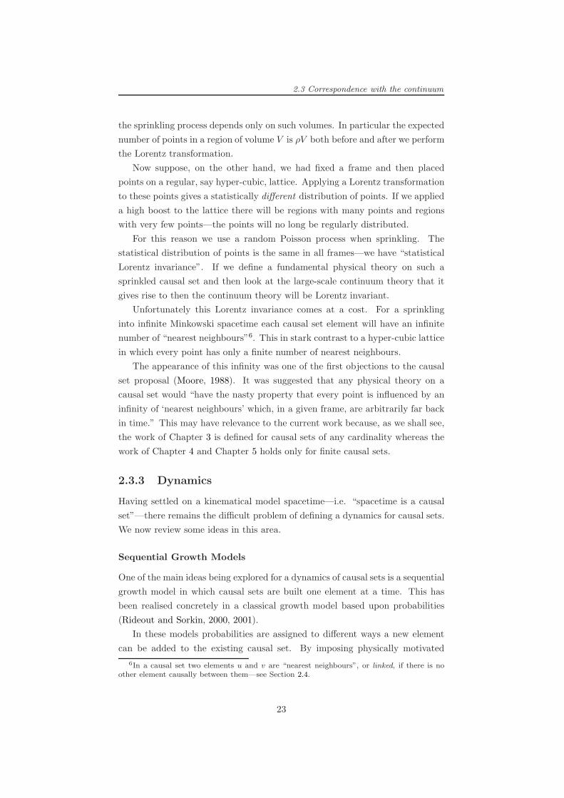
2.3.3 Dynamics
Having settled on a kinematical model spacetime—i.e. “spacetime is a causal
set”—there remains the difficult problem of defining a dynamics for causal sets.
We now review some ideas in this area.
Sequential Growth Models
One of the main ideas being explored for a dynamics of causal sets is a sequential
growth model in which causal sets are built one element at a time. This has
been realised concretely in a classical growth model based upon probabilities
(Rideout and Sorkin, 2000, 2001).
In these models probabilities are assigned to different ways a new element
can be added to the existing causal set. By imposing physically motivated
6In a causal set two elements u and v are “nearest neighbours”, or linked, if there is noother element causally between them—see Section 2.4.
23

2.4 Definitions
requirements on the probability assignments all possible probability rules can
be parametrised. By building causal sets in this way probabilities are assigned
to partial finite causal sets or, by running the process to infinity, to countably
infinite causal sets.
These classical sequential growth models were envisaged as a “classical warm-
up” to be replaced one day by a quantum mechanical model. The most naıve
attempt to do so would replace the real probabilities with complex probability
amplitudes. This would allow interference between the amplitudes which, it is
hoped, would allow large manifold-like causal sets to emerge (this is considered
in Dowker et al. (2010, §4)).Surprisingly, given its interim status, there is evidence that one type of
classical sequential growth model generates causal sets which are similar to 4-
dimensional de Sitter spacetime (Ahmed and Rideout, 2009).
Einstein-Hilbert action and Ricci Scalar
More recent work has attempted to find an action principle for causal sets. The
idea is to find a causal set analog of the 4-dimensional Einstein-Hilbert action.
This has been achieved by Benincasa and Dowker (2010). The causal set action
is a combinatorial sum of weights assigned to sub-structures in the causal set.
The expression for the action for a causal set C is (Benincasa and Dowker,
2010, eq (14)):
S(4)[C] = N −N1 + 9N2 − 16N3 + 8N4, (2.3)
where N is the number of elements in C and Ni is the number of (i+1)-element
causal intervals in C.While further work is needed on this approach it is hoped that this ac-
tion (presumably used in a quantum mechanical sum-over-histories formalism)
would enforce the causal sets to be large, four-dimensional and even solutions
to Einstein’s equations.
2.4 Definitions
It is worthwhile to gather together some definitions and notation which will
be used extensively later on in this work (we have already seen some of these
definitions, e.g. that of a causal interval). Good references include Stanley
(1986, Chapter 3).
If u v and u 6= v we write u ≺ v (we shall refer to this irreflexive relation
≺ as a strict causal relation). If u, v ∈ C are unrelated (meaning u 6 v and
v 6 u) we write u||v.
24

2.5 Representing causal sets
A pair (Q,′) is a sub-poset of a poset (P,) if Q is a subset of P and
the order relation ′ is equal to when restricted to elements in Q: i.e. u ′
v ⇐⇒ u v for all u, v ∈ Q.
An interval (or causal interval or Alexandrov set) is the set [u, v] := w ∈ C :
u w v whenever u ≺ v. Note that with this convention the “end-points”
of the interval are included: u, v ∈ [u, v]. Also [u, u] = u.A labelling assigns an integer subscript to the elements of C: labelling them
as vx for x = 1, . . . , |C|. A natural labelling is a labelling such that vx vy =⇒x ≤ y.
A total order (or totally ordered set or chain) is a partial order in which any
two elements are related—that is, there are no unrelated pairs of elements. One
familiar example of a total order is (Z,≤), i.e. the integers under the usual “less
than or equal to” order relation.
A subset of a causal set (C,) is a chain if it is totally ordered when regarded
as a sub-poset of (C,). A finite chain of length n is a sequence of distinct
elements u0 ≺ u1 ≺ u2 ≺ . . . ≺ un. A multichain is a chain with repeated
elements. A multichain of length n is a sequence of (not necessarily distinct)
elements u0 u1 u2 . . . un. An antichain is a set of elements which are
mutually unrelated.
A link (or covering relation or nearest neighbour relation) is a relation u ≺ v
such that there exists no w ∈ C with u ≺ w ≺ v. We say u and v are nearest
neighbours (or v covers u) and write u ≺∗ v. A path is a subset P ⊂ C which
is a maximal (or saturated) chain. This means P is a chain with no element
w ∈ C − P such that u ≺ w ≺ v for some u, v ∈ P . A finite path of length n is
a sequence of distinct elements u0 ≺∗ u1 ≺∗ u2 ≺∗ . . . ≺∗ un.A linear extension of a causal set (C,) is a total order (C,≤) which is
consistent with the partial order. This means u v =⇒ u ≤ v for all u, v ∈ C.The direct (or Cartesian) product of two partial orders (C1,1) and (C2,2)
is the partial order (C1 × C2,) based on the Cartesian product of the sets C1and C2 with order relation (u1, u2) (v1, v2) ⇐⇒ u1 1 v1 and u2 2 v2.
A set of elements v1, . . . , vn will be called non-Hegelian if they are mutually
unrelated and have identical (strict) causal relations to the rest of the causal
set. That is (u ≺ vx ≺ w) ⇐⇒ (u ≺ vy ≺ w) for all x, y = 1, . . . , n.
2.5 Representing causal sets
A finite causal set (C,) can be represented in a number of equivalent ways.
One way it to simply list the elements of C together with the order relations.
25

2.5 Representing causal sets
An example causal set we shall use to illustrate the different representations is:
C = v1, v2, v3, v4, v5, v6, (2.4)
v1 v1, v1 v2, v1 v3, v1 v4, v1 v5, v1 v6
v2 v2, v2 v3, v2 v5, v2 v6
v3 v3, v3 v5, v3 v6
v4 v4, v4 v5,
v5 v5,
v6 v6.
(2.5)
One can verify almost mechanically that this pair (C,) satisfy the four condi-
tions of a causal set.
2.5.1 Hasse diagrams and directed graphs
Another way to represent a finite causal set is by a Hasse diagram. Here the
elements of C are drawn as points in the page and if two elements are linked
u ≺∗ v then u is positioned lower than v with a line drawn connecting them (see
Figure 2.2).
Figure 2.2: The example causal set drawn as a Hasse diagram.
A similar, but ultimately more cluttered, approach is to draw the causal set
as a directed graph. Here elements are again drawn as points in the page but
all relations (not just links) between distinct elements are drawn in. A relation
26
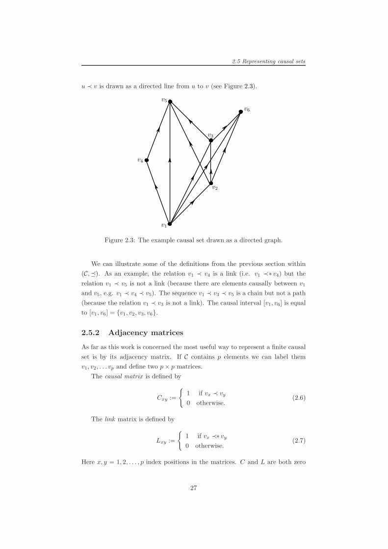
2.5 Representing causal sets
u ≺ v is drawn as a directed line from u to v (see Figure 2.3).
Figure 2.3: The example causal set drawn as a directed graph.
We can illustrate some of the definitions from the previous section within
(C,). As an example, the relation v1 ≺ v4 is a link (i.e. v1 ≺∗ v4) but the
relation v1 ≺ v5 is not a link (because there are elements causally between v1
and v5, e.g. v1 ≺ v4 ≺ v5). The sequence v1 ≺ v3 ≺ v5 is a chain but not a path
(because the relation v1 ≺ v3 is not a link). The causal interval [v1, v6] is equal
to [v1, v6] = v1, v2, v3, v6.
2.5.2 Adjacency matrices
As far as this work is concerned the most useful way to represent a finite causal
set is by its adjacency matrix. If C contains p elements we can label them
v1, v2, . . . vp and define two p× p matrices.
The causal matrix is defined by
Cxy :=
1 if vx ≺ vy
0 otherwise.(2.6)
The link matrix is defined by
Lxy :=
1 if vx ≺∗ vy0 otherwise.
(2.7)
Here x, y = 1, 2, . . . , p index positions in the matrices. C and L are both zero
27

2.5 Representing causal sets
on the main diagonal and, from the definition of a causal set, the labelling can
always be chosen to ensure they are both strictly upper triangular matrices (in
which case the labelling is a natural labelling).
One way to calculate L from C is to compute
L = C − (C2 > 0), (2.8)
where, for a real matrix A, (A > 0)xy = 1 if Axy > 0 and 0 otherwise.
If (C1,1) and (C2,2) are two finite causal sets with causal matrices C1
and C2, the direct product (C1 × C2,) (see Section 2.4) has causal matrix
(I + C1)⊗ (I + C2)− I ⊗ I = C1 ⊗ C2 + C1 ⊗ I + I ⊗ C2. (2.9)
where ⊗ denotes the Kronecker product.
Example
For our example causal set (C,) (defined in (2.4) and (2.5)) we have:
C =
0 1 1 1 1 1
0 0 1 0 1 1
0 0 0 0 1 1
0 0 0 0 1 0
0 0 0 0 0 0
0 0 0 0 0 0
, L =
0 1 0 1 0 0
0 0 1 0 0 0
0 0 0 0 1 1
0 0 0 0 1 0
0 0 0 0 0 0
0 0 0 0 0 0
. (2.10)
Chain lengths
Powers of these matrices have the following useful properties (Stanley, 1986,
p115):
(Cn)xy = The number of chains of length n from vx to vy, (2.11)
(Ln)xy = The number of paths of length n from vx to vy, (2.12)
((I + C)n)xy = The number of multichains of length n from vx to vy, (2.13)
(where I is the p× p identity matrix).
We can can appreciate why these formulae hold by considering the C2 ex-
ample. Here we have
(C2)xy :=
p∑
a=1
CxaCay. (2.14)
For each a = 1, . . . , p the summand is only non-zero if there exists a chain
vx ≺ va ≺ vy. When such a chain exists the summand is equal to 1. Thus
28

2.5 Representing causal sets
the sum is equal to the number of chains of length 2 from vx to vy. A similar
argument applies for other powers of C and L.
For finite causal sets both C and L are nilpotent matrices (meaning that
raising them to a high enough power gives the zero matrix). This means that
power series in C and L truncate. For example for a complex number z we have
D(z) := (I − zC)−1 = I + zC + (zC)2 + . . . =
∞∑
n=0
(zC)n, (2.15)
E(z) := exp(zC) = I + zC +(zC)2
2+ . . . =
∞∑
n=0
(zC)n
n!. (2.16)
where exp(zC) is the matrix exponential of zC and both power series truncate
(eventually).
We see that D(z)xy and E(z)xy are polynomials in z with degree equal to
the length of the longest chain from vx to vy. One way to calculate this degree is
to make use the following easily verified formula for the degree of a polynomial
P (z):
deg(P ) = limz→∞
zP ′(z)
P (z), (2.17)
where P ′ is the derivative of P .
Using this the length of the longest chain from vx to vy is equal to
limz→∞
zD(z)′xyD(z)xy
= limz→∞
z(CD(z)2)xyD(z)xy
= limz→∞
zE(z)′xyE(z)xy
= limz→∞
z(CE(z))xyE(z)xy
,
(2.18)
where we’ve used D(z)′ = CD(z)2 and E(z)′ = CE(z).
In numerical simulations substituting a large, but finite, value of z gives a
good approximation to the length of the longest chain.
We mention an interesting result for calculating the total number of chains
(or paths) of different lengths in a finite causal set. We have (Stanley, 1996),
for a finite causal set (C,) with causal matrix C and link matrix L:
The coefficient of zn in det(I + z(J −C)) (resp. det(I + z(J − L)))
is the total number of chains (resp. paths) of length n in C.
Here J is the “all ones” matrix: Jxy = 1 for x, y = 1, . . . , p.
29

2.5 Representing causal sets
Volumes
Squaring I + C or C can be used to compute the cardinality of the causal
intervals in the causal set. We have:
|[vx, vy]| = |w ∈ C|vx w vy| = ((I + C)2)xy, (2.19)
|w ∈ C|vx ≺ w ≺ vy| = (C2)xy. (2.20)
These cardinalities are just dimensionless numbers. If we assign a fundamen-
tal spacetime volume7 V0 to all causal set elements then the spacetime volume
of a region with N elements is equal to NV0.
If the volume of the causal set elements are not all equal8 (e.g. if one element
is regarded as having twice the spacetime volume of another, say) then we can
define a diagonal matrix V such that Vxx is the volume of element vx. We then
have
Vol([vx, vy]) = ((I + C)V (I + C))xy . (2.21)
7Which, presumably, should have a mass-dimension of [V0] = M−d if the causal set corre-sponds to a d-dimensional spacetime.
8We mention this for completeness although it goes against the spirit of the causal setapproach in which volume simply is number.
30

Chapter 3
Path Integrals
An electron has an amplitude to go from point to point in space-
time, which I will call “E(A to B).” Although I will represent E(A
to B) as a straight line between two points, we can think of it as
the sum of many amplitudes — among them, the amplitude for the
electron to change direction at points C or C′ on a “two-hop” path,
and the amplitude to change direction at D and E on a “three-hop”
path—in addition to the direct path from A to B. The number
of times an electron can change direction is anywhere from zero to
infinity, and the points at which the electron can change direction
on its way from A to B in space-time are infinite. All are included
in E(A to B).
Richard Feynman, (1985, p92)
In this chapter we describe an approach to modelling particles on a causal set.
The main results are a collection of models for defining discrete path integrals
on a causal set. These lead to propagators for particles on a causal set which,
in a suitable sense, match the continuum propagators when the causal set is
generated by sprinkling into Minkowski spacetime.
The main results of this chapter appear in Johnston (2008a, 2009b). One of
the models also appears in a Wolfram demonstration (Johnston, 2008b).
3.1 Particle models
The question of how to model matter on a causal set has been addressed by a
number of people. As a result there are a number of different models, each using
different physical and mathematical ideas. Here we review the models which
31

3.1 Particle models
treat matter as particles rather than fields (fields will be addressed in Chapter
4).
3.1.1 Swerves
In general relativity free classical point particles follow geodesics in spacetime.
It is tempting to use this geometrical rule to model free point particles on a
causal set. The most studied models of this type are the swerves models. The
first of these was proposed by Dowker et al. (2004) to model a massive point
particle.
The idea behind this approach is to find a Markovian propagation rule that
determines the worldline trajectory of a point particle. The trajectory is built
up iteratively, one element at a time, with the next element being chosen by
applying the rule. The rule depends on the structure of the causal set as well as
the past trajectory of the particle (either the entire past trajectory or the past
trajectory only up to some finite “forgetting time”).
The aim is to find a rule such that the large-scale behaviour of a massive
point particle when propagating on a sprinkled causal set is to follow a timelike
geodesic. Of course, for a particular sprinkled causal set, this will not be possible
exactly due to the random distribution of sprinkled points. In general the
particle will be forced to swerve slightly as it attempts to hug a geodesic as
closely as possible. It is this swerving behaviour that gives the approach its
name and would provide a clear signal of underlying spacetime discreteness.
A number of swerves models have been developed which give the correct
large-scale geodesic behaviour (see Philpott et al. (2009); Philpott (2009, 2010)
for full details).
The phenomenology of these models has focussed on their effect on particle
propagation when the continuum limit is taken. It turns out that, so long as
the underlying propagation rule is Lorentz-invariant, the continuum behaviour
is described by a Lorentz-invariant diffusion equation depending on the mass of
the particle and a “diffusion parameter”. By comparing this continuum descrip-
tion to experiments and observations the size of the diffusion parameter can be
constrained.
This continuum description can be modified to describe massless particles
(Philpott et al., 2009, Sec IV) as well as massless particles with polarisation
(Contaldi et al., 2010) (e.g. photons from the cosmic microwave background).
In these massless cases, however, there is, at yet, no underlying causal set prop-
agation rule that leads to the continuum description.
32

3.1 Particle models
3.1.2 Hemion classical model
In the Hemion model for discrete spacetime (Hemion (1980, Sec 2), Hemion
(1988, Sec 3.4)) particles are modelled as infinite chains—infinite totally or-
dered sets of spacetime points which represent the particle’s worldline. The
particles in this model are classical and cannot be created or destroyed. Nev-
ertheless Hemion acknowledges that future developments could lead to a model
that includes quantum behaviour such as “the phenomena of creation and an-
nihilation, vacuum loops, and in general all the particle structures normally
considered in Feynman diagrams” (p1181).
To accommodate these classical particles it is assumed that the posetW has
“particle structure”, meaning it is the disjoint union of totally ordered subsets.
The elements of W then make up the particle worldlines and points in empty
space are “positions” in W (Hemion, 1988, Sec 3.6).
In Hemion (1988) he focuses on defining an interacting point particle model
for classical electrodynamics. This is done within the Fokker action-at-a-distance
framework for classical electrodynamics (which we shall return to in Section
3.14.3).
3.1.3 Discrete path integrals
The two models just described suffer the serious draw-back that they are entirely
classical. This is problematic when seeking a fundamental model for matter at
ultra-small length scales because on such scales the effects of quantum mechanics
are very important. On small scales it is simple incorrect to model matter as
a collection of classical point particles with precisely defined, unique spacetime
worldlines1.
A better approach is to base the particle model on quantum mechanics from
the outset. The work presented here does just this by basing the model on the
path-integral formulation of quantum mechanics.
The path integral approach was initiated by Dirac (1933) and ultimately
brought to completion by Feynman (1948c). A full introduction is given in
Feynman and Hibbs (1965) and a very readable introduction for the lay-person
is given in Feynman (1985).
In this formulation the “propagator” for a point particle is given centre stage.
This is a complex valued function of two spacetime points which describes the
quantum mechanical propagation of the particle. In the path integral formalism
it is obtained as a quantum mechanical path integral. Complex probability
1It remains possible, however, that quantum mechanics emerges from a deeper deterministictheory (see, e.g. ’t Hooft (2006)). In this case, however, the deterministic objects in the deepertheory would not correspond to the particles in the emergent quantum mechanics.
33

3.2 Causal set path integrals
amplitudes are assigned to all possible trajectories that the particle can take
and, by summing these amplitudes up over all trajectories, the propagator is
obtained.
That, in principle, is the idea. When it comes to calculating this path inte-
gral for, say, a non-relativistic particle in the continuum, there are unwelcome
mathematical difficulties which arise. Since the amplitudes are complex num-
bers the path integral cannot be defined as a bone fide integral over a space of
paths. Instead the path “integral” is really a prescription for 1) discretising the
paths, 2) performing the path integral over skeletonised paths and 3) the taking
the continuum limit.
If spacetime is not a continuum then perhaps these mathematical difficulties
can be overcome, perhaps the sum over particle paths can be defined directly
and rigorously. Indeed, if spacetime is modelled as a causal set then, as we shall
see, this is precisely what happens.
We mention that path integrals on discrete spacetime have been considered
before. In Gudder (1988), for example, path integrals on a hyper-cubic lattice
were described. The idea of path integrals on causal sets was considered by
Meyer (1997) but unfortunately never developed. Some work with propagators
on a causal set has been done by Daughton (1993); Salgado (2008); Sorkin (2009)
(see Section 4.3.1 for a summary). Discrete path integral models have also been
inspired by the Feynman checkerboard model (see Section 6.3 for details).
As it turns out, a very similar approach to the one described in this chapter
was developed independently as a summer project at the University of San Jose
(the results of which appeared in Scargle and Simic (2009)). Their aim was
to develop a model for the effect of spacetime discreteness on photon energy.
The result was a path integral model for photons which took the “sum over all
paths” spirit of the formulation literally—the paths summed over in their model
include future-directed, past-directed and spacelike paths.
3.2 Causal set path integrals
To define path integrals on a causal set we have to make two choices: which
trajectories to sum over and what amplitudes to assign to each trajectory. The
two most obvious choices for trajectories are all chains between two elements or
all paths between two elements.
Since the causal set is locally finite there are only a finite number of chains or
paths between any two elements. Assigning each one an appropriate amplitude
we can then simply sum the amplitudes to obtain the propagator. For every
pair of elements this sum will exist since we are just summing a finite collection
of complex numbers. We must then attempt to choose amplitudes which give
34
3.2 Causal set path integrals
us the correct propagator.
We shall present a number of different models, each suitable for obtaining
a different continuum propagator when the causal set is generated by sprin-
kling into Minkowski spacetime of different dimensions. In all the models the
amplitude assigned to each trajectory depends on the length of the trajectory.
3.2.1 The models
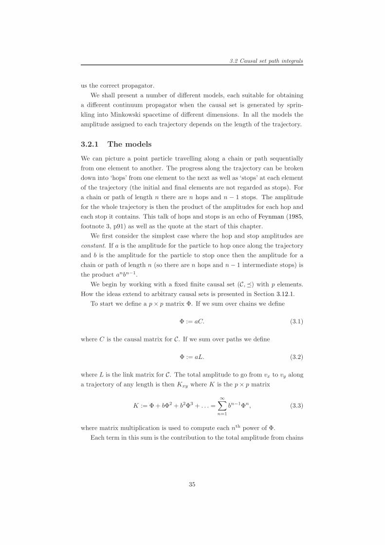
We can picture a point particle travelling along a chain or path sequentially
from one element to another. The progress along the trajectory can be broken
down into ‘hops’ from one element to the next as well as ‘stops’ at each element
of the trajectory (the initial and final elements are not regarded as stops). For
a chain or path of length n there are n hops and n − 1 stops. The amplitude
for the whole trajectory is then the product of the amplitudes for each hop and
each stop it contains. This talk of hops and stops is an echo of Feynman (1985,
footnote 3, p91) as well as the quote at the start of this chapter.
We first consider the simplest case where the hop and stop amplitudes are
constant. If a is the amplitude for the particle to hop once along the trajectory
and b is the amplitude for the particle to stop once then the amplitude for a
chain or path of length n (so there are n hops and n− 1 intermediate stops) is
the product anbn−1.
We begin by working with a fixed finite causal set (C,) with p elements.
How the ideas extend to arbitrary causal sets is presented in Section 3.12.1.
To start we define a p× p matrix Φ. If we sum over chains we define
Φ := aC. (3.1)
where C is the causal matrix for C. If we sum over paths we define
Φ := aL. (3.2)
where L is the link matrix for C. The total amplitude to go from vx to vy along
a trajectory of any length is then Kxy where K is the p× p matrix
K := Φ + bΦ2 + b2Φ3 + . . . =
∞∑
n=1
bn−1Φn, (3.3)
where matrix multiplication is used to compute each nth power of Φ.
Each term in this sum is the contribution to the total amplitude from chains
35
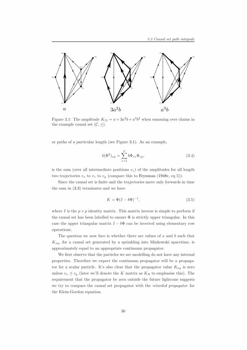
3.3 Causal set path integrals
Figure 3.1: The amplitude K15 = a+3a2b+ a3b2 when summing over chains inthe example causal set (C,).
or paths of a particular length (see Figure 3.1). As an example,
b(Φ2)xy =
p∑
z=1
bΦxzΦzy, (3.4)
is the sum (over all intermediate positions vz) of the amplitudes for all length
two trajectories vx to vz to vy (compare this to Feynman (1948c, eq 5)).
Since the causal set is finite and the trajectories move only forwards in time
the sum in (3.3) terminates and we have
K = Φ(I − bΦ)−1, (3.5)
where I is the p× p identity matrix. This matrix inverse is simple to perform if
the causal set has been labelled to ensure Φ is strictly upper triangular. In this
case the upper triangular matrix I − bΦ can be inverted using elementary row
operations.
The question we now face is whether there are values of a and b such that
Kxy, for a causal set generated by a sprinkling into Minkowski spacetime, is
approximately equal to an appropriate continuum propagator.
We first observe that the particles we are modelling do not have any internal
properties. Therefore we expect the continuum propagator will be a propaga-
tor for a scalar particle. It’s also clear that the propagator value Kxy is zero
unless vx vy (later we’ll denote the K matrix as KR to emphasise this). The
requirement that the propagator be zero outside the future lightcone suggests
we try to compare the causal set propagator with the retarded propagator for
the Klein-Gordon equation.
36
3.3 Propagators in the continuum
3.3 Propagators in the continuum
The propagators in d-dimensional Minkowski spacetime scalar quantum field
theory are Green’s functions of the Klein-Gordon equation:
(+m2)G(d)m (x) = δd(x). (3.6)
Here x = (x0, ~x), m is the mass of the particle, δd is the d-dimensional Dirac
delta function and we choose units with ~ = c = 1. The d’Alembertian is given
by
:=∂2
∂x02− ∂2
∂x12− ∂2
∂x22− . . .− ∂2
∂xd−12. (3.7)
We can think of G(d)m (x) as the propagation amplitude for the particle to travel
from the origin to x ∈ Md. More generally, using the translation-invariance of
Md, G(d)m (y − x) is the propagation amplitude for the particle to travel from x
to y (in curved spacetimes the propagator depends on x and y separately, see
Section 3.13.2).
To obtain the propagator G(d)m (x) explicitly we define the Fourier transform
by
f(p) :=
∫ddxf(x)eipx, f(x) =
1
(2π)d
∫ddpf(p)e−ipx, (3.8)
where px := p0x0 − ~p · ~x. Using this we can solve equation (3.6) to obtain
G(d)m (p) := − 1
p20 − ~p2 −m2, (3.9)
so
G(d)m (x) := − 1
(2π)d
∫ddp
e−ipx
p20 − ~p2 −m2. (3.10)
The mass-dimension of this propagator is [G(d)m ] =Md−2.
The integrand in these expressions contains poles so the Minkowski space-
time propagator is only uniquely defined if we specify a contour of integration
or, equivalently, boundary conditions for the solution of (3.6). The retarded
propagator, which we’ll denote (GR)(d)m (x), is the unique Green’s function which
is only non-zero in the future lightcone—that is, (GR)(d)m (y − x) is zero unless
x y.
This boundary condition can be imposed by avoiding the poles in (3.9) at
p0 = ±√~p2 +m2 by two small semi-circles in the upper-half p0 complex plane.
This is equivalent to
(GR)(d)m (x) := lim
ǫ→0+− 1
(2π)d
∫ddp
e−ipx
(p0 + iǫ)2 − ~p2 −m2. (3.11)
37

3.4 Propagators in the continuum
This integral can be evaluated in various dimensions. The rigorous calcu-
lations require the use of the theory of distributions (See Gel’fand and Shilov
(1964) for the general theory and De Jager, E.M. (1967) for the theory applied
in detail to the d = 4 Klein-Gordon equation).
We list the expressions2 for dimensions d = 1, 2, 3, 4:
(GR)(1)m (x) = θ(x0)
sin(mx0)
m(3.12)
(GR)(2)m (x) = θ(x0)θ(τ2)
1
2J0(mτ) (3.13)
(GR)(3)m (x) = θ(x0)θ(τ2)
1
2π
cos (mτ)
τ(3.14)
(GR)(4)m (x) = θ(x0)θ(τ2)
(1
2πδ(τ2)− m
4π
J1(mτ)
τ
)(3.15)
Here τ :=√(x0)2 − ~x2 is the proper length of the vector x, Jα is a Bessel
function of the first kind of order α, δ is the Dirac delta function and
θ(α) =
1 if α ≥ 0
0 if α < 0.(3.16)
For a comprehensive introduction to Bessel functions the reader is directed to
the classic Watson (1958).
For ease of reference we list the massless (GR)(d)0 propagators3 (which are
simply obtained by taking the m→ 0 limit of each (GR)(d)m ):
(GR)(1)0 (x) = θ(x0)x0 (3.17)
(GR)(2)0 (x) = θ(x0)θ(τ2)
1
2(3.18)
(GR)(3)0 (x) = θ(x0)θ(τ2)
1
2πτ(3.19)
(GR)(4)0 (x) = θ(x0)θ(τ2)
1
2πδ(τ2) (3.20)
The advanced propagator (GA)(d)m (x) is obtained from the boundary condi-
tions that it be non-zero only in the past lightcone. It is related to the retarded
propagator by (GA)(d)m (x) = (GR)
(d)m (−x). The Feynman propagator is obtained
by more complicated boundary conditions—see Section 4.4.1 for details.
2(GR)(1)m is obtained by a straightforward calculation from (3.11). The expressions for
(GR)(d)m with d = 2, 3, 4 are given in Egorov and Shubin (1994, Example 2.3, p144-145). The
physical 4-dimensional case is covered in great detail in Bogoliubov and Shirkov (1959, §15)and De Jager, E.M. (1967).
3These are also given in Egorov and Shubin (1994, Example 2.2, p144).
38

3.5 Dimensional analysis
3.4 Dimensional analysis
If we wish the causal set propagators to match the Klein-Gordon propagators
then, of course, their mass-dimensions should be the same. This simple condi-
tion can help to constrain the form of the a and b amplitudes.
Firstly we observe that the amplitudes anbn−1 must all have equal mass-
dimension (since we are adding them together) for n = 1, 2, . . .. This implies
that [ab] = 1, that is, the product ab is dimensionless.
Now, in d-dimensional Minkowski spacetime the mass-dimension of the Klein-
Gordon propagators are [G(d)m ] = Md−2. Matching this to [anbn−1] for all n
gives:
[a] =Md−2 [b] =M2−d [ab] = 1. (3.21)
The only dimensionful quantities available to use on a sprinkled causal set are
the sprinkling density ρ and the mass of the particle m. These satisfy
[ρ] =Md [m] =M. (3.22)
This is as far as we can go without additional assumptions—there are a number
of ways of combining ρ and m to create amplitudes with dimensions Md−2 and
M2−d.
If, however, we assume that a is independent of the particle mass then a
must only depend on ρ. This fixes the form of a to be
a = Aρ1−2/d, (3.23)
where A is a dimensionless constant. As it turns out our a amplitudes will have
this form.
3.5 Expected values
Causal sets generated by sprinklings into a Lorentzian manifold will not be
identical because the particular points that are sprinkled are chosen randomly.
The value of the propagator calculated from one sprinkled causal set therefore
depends in detail on the particular causal set that is generated. To compare
the causal set and continuum propagators we shall be interested in the expected
value (and variance) for the causal set propagator calculated by averaging over
all possible sprinkled causal sets.
To understand why, suppose we model spacetime by a causal set generated
by sprinkling into Md with density ρ. For all pairs of sprinkled points we can
calculate the causal set propagator by summing over trajectories in the manner
39

3.5 Expected values
described in Section 3.2. We can also compute the continuum propagator for
all pairs of points (using their coordinates in Md and the formulae in Section
3.3). We then wish to compare these two sets of propagator values. In addition
we wish to compare the values for a typical sprinkling, not just the particular
causal set we sprinkled. To do this we will compute the expected value of the
causal set propagator and compare it to the continuum propagator.
To compute the expected values for sprinklings into d-dimensional Minkowski
spacetime we first fix two points x, y ∈ Md. We then sprinkle a causal set. There
is zero probability that the sprinkled causal set will contain x and y so we then
add x and y to the sprinkled causal set. We then count the number of chains
and paths and calculate the value of the propagator between the two points.
Averaging these values over all sprinkled causal sets (with a fixed sprinkling
density ρ), we obtain the expected number of chains and paths from x to y and
the expected value of the propagator between x and y.
3.5.1 Summing over chains
To calculate the expected number of chains between two points x and y in
d-dimensional Minkowski spacetime we define4
C(y − x) :=
1 if x y
0 otherwise.(3.24)
Translation invariance of Minkowski spacetime ensures C(y− x) is only a func-
tion of the separation y− x. The expected number of chains of length one from
x to y is given by
C1(y − x) = C(y − x). (3.25)
The expected number of chains x ≺ z1 ≺ . . . ≺ zn−1 ≺ y of length n > 1 is
given by Meyer (1988, p49-50):
Cn(y−x) := ρn−1
∫· · ·∫ddz1 · · · ddzn−1C(y−zn−1)C(zn−1−zn−2) · · ·C(z1−x).
(3.26)
This integral can be evaluated in closed form (Meyer, 1988, Theorem III.2, p50).
For n > 1 we have:
Cn(y − x) = C(y − x)(ρV (x− y))n−1
n− 1
(Γ(d+ 1)
2
)(n−2)Γ(ω)Γ(2ω)
Γ((n− 1)ω)Γ(nω),
(3.27)
4This function on Md should not be confused with the causal matrix Cxy.
40
3.5 Expected values
where5 ω := d/2 and V (x− y) = V (y− x) denotes the d-dimensional volume of
the causal interval between x and y and Γ(z) is the Gamma function.
In general we have, (Rideout and Zohren, 2006, eq (44)):
V (x− y) =π
d−1
2
2d−1dΓ((d+ 1)/2)τd, (3.28)
where τ is the proper time from x to y.
The expected value for a propagator which sums amplitudes assigned to
chains is given by
KC(y − x) :=
∞∑
n=1
anbn−1Cn(y − x). (3.29)
This satisfies the integral equation
KC(y − x) = aC(y − x) + abρ
∫ddz C(y − z)KC(z − x). (3.30)
3.5.2 Summing over paths
To calculate the expected number of paths between two sprinkled points x and
y in d-dimensional Minkowski spacetime we define
P (y − x) :=
e−ρV (x−y) if x y
0 otherwise.(3.31)
where V (x− y) is the d-dimensional Minkowski spacetime volume of the causal
interval between x and y. The expected number of paths of length one from x
to y (i.e. the probability that x ≺∗ y) is given by
P1(y − x) = P (y − x). (3.32)
The expected number of paths x ≺∗ z1 ≺∗ . . . ≺∗ zn−1 ≺∗ y of length n > 1 is
given by (Bombelli, 1987, eq 2.5.5, p75):
Pn(y−x) = ρn−1
∫· · ·∫ddz1 · · · ddzn−1P (y−zn−1)P (zn−1−zn−2) · · ·P (z1−x).
(3.33)
Unfortunately no closed-form expression is known for Pn(y−x) for general n and
d (although an attempt is made to find an asymptotic form for the expectation
of the total number of paths for sprinklings into M2 in Bombelli (1987, p76-77).
5The notation in Meyer (1988) is different to that used here. His d refers to the spatial
dimension (i.e. our d minus 1), he sets ρ = 1 and he writes 〈Ck〉 to denote the expectednumber of chains of length k + 1 (i.e. 〈Cn−1〉 = Cn(x− y)).
41

3.6 1+1 dimensional Minkowski spacetime
In Appendix A we attempt to determine Pn as fully as possible).
The expected value for the propagator which sums over paths is given by
KP (y − x) :=
∞∑
n=1
anbn−1Pn(y − x). (3.34)
This satisfies the integral equation
KP (y − x) = aP (y − x) + abρ
∫ddz P (y − z)KP (z − x). (3.35)
3.6 1+1 dimensional Minkowski spacetime
It turns out (in the sense that we get the right answer) that in 1+1 dimensions
the propagator requires us to sum over chains.
3.6.1 Fourier transform calculation
Fourier transforming (3.30) the integral, being a convolution, becomes a product
and we have
KC(p) = aC(p) + abρ C(p)KC(p), (3.36)
or
KC(p) =aC(p)
1− abρC(p). (3.37)
In 1+1 dimensions the function C(x) has Fourier transform
C(p) = − 2
(p0 + iǫ)2 − p21, (3.38)
since C(x) = 2(GR)(2)0 (x) (and setting m = 0 in (3.9)). Substituting this into
(3.37) we have
KC(p) =− 2a
(p0+iǫ)2−p21
1 + 2abρ(p0+iǫ)2−p2
1
= − 2a
(p0 + iǫ)2 − p21 + 2abρ. (3.39)
Equating this to the d = 2 version of equation (3.9) we find
a =1
2, b = −m
2
ρ, (3.40)
are the correct amplitudes.
In 1+1 dimensions [ρ] = M2 so the amplitudes assigned to the chains are
dimensionless: [a] = [b] = [anbn−1] = 1 (for n = 1, 2, . . .).
42

3.7 3 + 1 dimensional Minkowski spacetime
3.6.2 Direct calculation
An alternative approach is to use the explicit form for Cn given in (3.27) to
calculate KC for sprinklings into 1+1 dimensions.
Using V (x− y) = τ2/2, d = 2 and substituting (3.27) into (3.29) we have:
KC(y − x) :=C(y − x)
(a+
∞∑
n=2
anbn−1ρn−1τ2n−2
(n− 1)2n−1
(Γ(3)
2
)(n−2)Γ(1)Γ(2)
Γ(n− 1)Γ(n)
),
(3.41)
=C(y − x)
(a+
∞∑
n=2
anbn−1ρn−1 1
2n−1Γ(n)Γ(n)τ2n−2
), (3.42)
=C(y − x)aI0
(√2abρ τ
), (3.43)
where I0 is a modified Bessel function of the first kind. This satisfies I0(iz) =
J0(z).
We thus see that with a = 1/2, b = −m2/ρ (so 2abρ = −m2) we have:
KC(y− x) = C(y− x)1
2I0(imτ) = C(y− x)
1
2J0(mτ) = (GR)
(2)m (y− x). (3.44)
3.7 3 + 1 dimensional Minkowski spacetime
It turns out that in 3+1 dimensions the propagator requires us to sum over
paths. Fourier transforming (3.35) we get
KP (p) =aP (p)
1− abρP (p). (3.45)
In 3+1 dimensional Minkowski spacetime V (x − y) := π24τ
4xy is the volume of
the causal interval between x and y. We therefore have
P (y − x) =
e−ρV (x−y) = e−
π24
ρτ4xy if x y
0 otherwise.(3.46)
The function
fρ(z, c) :=
√ρe−πcρz2
if z ≥ 0
0 if z < 0,(3.47)
(with a real constant c > 0) satisfies
limρ→∞
fρ(z, c) =1
2√cδ(z), (3.48)
43

3.7 3 + 1 dimensional Minkowski spacetime
where δ(z) is the Dirac delta function6. We therefore see
limρ→∞
√ρP (y−x) = lim
ρ→∞
fρ(τ
2xy,
124 ) if x0 ≤ y0
0 otherwise=
√242 δ(τ2xy) if x y
0 otherwise.
(3.49)
Setting m = 0 in (3.9) and using (3.20) we see that in 3+1 dimensions we have
(GR)(4)0 (y − x) =
12π δ(τ
2xy) if x y
0 otherwise,(3.50)
(GR)(4)0 (p) = − 1
(p0 + iǫ)2 − ~p2. (3.51)
These imply, taking Fourier transforms and using (3.49), that7
limρ→∞
√ρ P (p) = 2π
√24
2(GR)
(4)0 (p) = −2π
√6
1
(p0 + iǫ)2 − ~p2. (3.52)
Setting
a = A√ρ, b =
B
ρ, (3.53)
where A and B are (possibly dimensionful) constants independent of ρ we sub-
stitute into (3.45) to get
KP (p) =A√ρP (p)
1−AB√ρP (p)
. (3.54)
As ρ tends to infinity this becomes
limρ→∞
KP (p) =− AC
(p0+iǫ)2−~p2
1 + ABC(p0+iǫ)2−~p2
= − AC
(p0 + iǫ)2 − ~p2 +ABC, (3.55)
where C := 2π√6.
Equating this with the d = 4 version of equation (3.9) we have
AC = 1, B = −m2, (3.56)
so
a =
√ρ
2π√6, b = −m
2
ρ, (3.57)
6This limit is in the sense of distributions (see Gel’fand and Shilov (1964, Example 2,p36-37)).
7 We make use of the fact that
limρ→∞
fρ = f ⇐⇒ limρ→∞
fρ = f
for suitable functions f (Champeney, 1989, Thm 13.2, p135).
44

3.8 Comparison with the continuum
are the correct amplitudes.
In 3+1 dimensions [ρ] = M4 so the amplitudes assigned to the paths have
mass-dimension M2: [a] =M2, [b] =M−2, [anbn−1] =M2 (for n = 1, 2, . . .).
3.7.1 Summing over chains
In 3+1 dimensions we have to sum over paths. We briefly mention what happens
if we sum over chains.
Setting d = 4 and substituting (3.27) into (3.29) we have:
KC(y − x) :=C(y − x)
a+
∞∑
n=2
anbn−1 (ρV )n−1
(Γ(5)2
)n−2
Γ(2)Γ(4)
(n− 1)Γ(2n− 2)Γ(2n)
,
(3.58)
=C(y − x)
(a+ a
∞∑
n=2
(abρV )n−1 (12)n−2 6
(n− 1)Γ(2n− 2)Γ(2n)
),
(3.59)
=C(y − x)a
c(I1(c) + J1(c)) , (3.60)
where c = 2(12abρV )1/4
While it may be of interest to know this result it does not seem possible to
find a and b such that (3.60) is equal to (GR)(4)m (even in the infinite ρ limit). It
is possible that summing over chains with different amplitudes (not of the form
anbn−1) may reproduce the continuum propagator (in a sense, this is what we
are doing when we sum over paths because every path is a chain).
3.8 Comparison with the continuum
The causal set propagators just described can be calculated for a particular
sprinkling using a computer. We can then compare the causal set and continuum
propagators with the following steps:
1. Fix a sprinkling density ρ and a particle mass m.
2. Sprinkle a causal set C with density ρ into a causal interval8 in Md.
3. Compute C and L, the causal and link matrices for C.
4. Compute KR, the propagator matrix.
8We use a causal interval to ensure that the causal structure of the causal set matches thatof Md—i.e. there are no edge effects such as sub-causal-intervals being “chopped off” by theedges of the region. Another way to say this is that a causal interval is causally convex (aregion R ⊂ Md is causally convex if x, y ∈ R =⇒ [x, y] ⊆ R.)
45
3.8 Comparison with the continuum
5. For each pair of causally related points vx vy compute their proper time
separation τxy using their coordinates in Md.
6. Plot (KR)xy against τxy for all pairs of related points and compare it with
(GR)(d)m as a function of proper time.
We now perform this comparison for sprinklings into 1+1 and 3+1 dimen-
sional Minkowski spacetime.
3.8.1 1+1 dimensions
In Section 3.6 we showed that the causal set propagator for sprinklings into M2
is given by:
KR :=1
2C
(I +
m2
2ρC
)−1
, (3.61)
(where we sum over chains and use the a and b amplitudes from (3.40)).
In Figure 3.2 and Figure 3.3 we plot this propagator for two sprinklings with
m = 10 and for ρ = 600 and ρ = 1200. Every dot that is plotted corresponds
to a pair of causally related sprinkled points. For that pair their proper time
separation τxy is the horizontal coordinate and the value of the propagator
(KR)xy is their vertical coordinate.
As we can see there is good agreement between the causal set propagator and
the continuum propagator. In general this agreement holds provided m2 ≪ ρ.
If m2 > ρ the plotted points are spread more widely away from the continuum
curve. In Figure 3.4 we plot the results for ρ = 600,m = 30. This has m2/ρ =
1.5 and shows poor agreement with the continuum. This behaviour suggests
that the variance of the propagator is small provided m2 ≪ ρ.
Since we are not plotting the expected value of the propagator, but rather
the propagator calculated for a single causal set, there are fluctuations away
from the continuum propagator. These appear as a spread in the dots away
from the (GR)(2)m curve. These fluctuations are due to the particular random
distribution of points used in the sprinkling. If we fix the mass and the volume
of the causal interval we find that these fluctuations decrease as the density is
increased. As an example of this we can compare the plots for ρ = 600 and
ρ = 1200—the spread of the plotted points in Figure 3.3 is less than in Figure
3.2.
For small proper times the causal set propagator becomes “discretised”—the
values clump into a few horizontal layers. This is because points separated by
a small proper time will only contain a few other points in the causal interval
between them. If this number is small (say 1,2,3 or 4) then there’s only a few
values the propagator can take (e.g. if the n points in between are mutually
46

3.8 Comparison with the continuum
Figure 3.2: The causal set retarded propagator for a sprinkling in 1+1 dimen-sions with ρ = 600,m = 10. Each dot corresponds to a pair of causally relatedsprinkled points.
Figure 3.3: The causal set retarded propagator for a sprinkling in 1+1 dimen-sions with ρ = 1200,m = 10.
47

3.8 Comparison with the continuum
Figure 3.4: The causal set retarded propagator for a sprinkling in 1+1 dimen-sions with ρ = 600,m = 30. There is poor agreement with the continuum form2 > ρ.
unrelated the propagator is a + na2b). When the proper time is larger there
are many more points contained in the causal interval and subsequently a larger
range of values for the propagator. This leads to the values becoming more
“smeared out” and not confined to a few layers. Another way to think about
this is that when we sum over a large number of paths there is more interference
between the amplitudes assigned to paths of different lengths.
3.8.2 3+1 dimensions
In Section 3.7 we showed that the causal set propagator for sprinklings into M4
is given by:
KR :=
√ρ
2π√6L
(I +
m2
2π√(6ρ)
L
)−1
, (3.62)
(where we sum over paths and use the a and b amplitudes from (3.57)).
When comparing this with the continuum, however, there are difficulties
which did not arise in the 1+1 dimensional case. Firstly, for sprinklings into
M4 the expected value of the propagator only equals the continuum propagator
in the infinite density limit. A realistic sprinkling density (e.g. at Planckian
density) would be large but finite. We therefore expect to get good agreement
only for very large sprinkling densities9.
9The sprinkling process is only defined for finite densities. It makes no sense to sprinkle
48

3.8 Comparison with the continuum
Investigating the behaviour of the propagator for large sprinkling densities
is difficult to do through numerical simulations. This is because current simu-
lations cannot cope with enough sprinkled points to ensure a large density over
a large spacetime volume.
High density sprinklings can be achieved, however, if we sprinkle a moderate
number of points into a small volume. Unfortunately in this case the behaviour
of the propagator is only investigated within such small volumes—i.e. for small
proper times. For the 3+1 dimensional case the small proper time behaviour
is dominated by the delta-function term in the propagator (which, for finite
densities, is smeared out away from the lightcone).
In Figure 3.5 we plot the propagator for a sprinkling into a small causal
interval with ρ = 480625,m = 10. The horizontal line present for small proper
times corresponds to the propagator value for pairs of linked elements. Its value
is a =√ρ/(2π
√6) ≈ 45. The other values present for larger proper times are
contributions from elements joined by paths of length greater than 1 (as in the
1+1 dimensional case these values are “discretised” into horizontal layers).
We do not yet see the Bessel function behaviour within the future lightcone
that is present in the continuum propagator (GR)(4)m . Presumably this behaviour
would be apparent if a simulation could be performed with a large sprinkling
density over a large spacetime volume. This is a task for future work.
Figure 3.5: The causal set retarded propagator for a sprinkling in 3+1 dimen-sions.
an “infinite density” causal set.
49

3.9 Mass scatterings
A second difficulty is that we cannot compare the two propagators directly.
The continuum propagator contains a delta-function term on the forward light-
cone. This is a distributional object which we cannot plot explicitly. One
solution to this would be to apply the continuum and causal set propagators to
a family of test functions and compare the results. We have not done this com-
parison since the current simulations suggest a much higher density is needed
to obtain good results.
We note that, extrapolating from the 1+1 dimensional case, we would ex-
pect good agreement with the continuum propagator (for very large ρ) provided
m2 ≪ √ρ. This constraint on the mass of the particle is easily satisfied for re-
alistic sprinkling densities. Assuming a Planckian sprinkling density we let ρ be
the inverse of the Planck 4-volume: ρ = c7/(G~)2. The heaviest known elemen-
tary particle is the top quark with a mass m = 171.3± 1.2GeV (Amsler et al.,
2008). In Planck units, so ρ = 1, this is m ≈ 1.4 × 10⁻¹⁷. This certainly
satisfies m2/√ρ ≈ 2 × 10⁻³⁴ ≪ 1. If the masses of particles modelled on the
causal set are of order the masses of known elementary particles then the causal
set propagator (for a Planckian density sprinkling) should well-approximate the
continuum propagator.
3.9 Mass scatterings
Having established suitable amplitudes for causal sets generated by sprinkling
into 1+1 and 3+1 dimensional Minkowski spacetime we can now better under-
stand why they take the values they do.
The mass dependence for both propagators is entirely contained in the am-
plitude b = −m2/ρ. By setting the mass to zero we see that the series for the
propagator truncates to give K = Φ where Φxy is just the amplitude for the
particle to ‘hop’ from vx to vy . We thus see that the hop amplitude for a massive
particle is equal to total propagation amplitude for a massless particle.
This suggests that a free massive particle is equivalent to a massless parti-
cle undergoing repeated “self-interactions” at each stop. The strength of these
interactions is governed by b. Through these “mass scatterings” the massless
propagator is “dressed up” to give the massive propagator. We have kept the
quotation marks since we have not yet developed a theory of interacting parti-
cles.
The same idea of a massless particle undergoing self-interaction mass scat-
terings can be dealt with in the continuum. To demonstrate this we suppose
that G0(x) is the massless propagator for the Klein-Gordon equation:
G0(x) = δd(x). (3.63)
50

3.10 Mass scatterings
Defining the d-dimensional convolution of two functions f and g on Md as
(f ∗ g)(x) :=∫ddyf(x− y)g(y), (3.64)
we now consider the function defined by
Gm(x) := G0(x)−m2(G0 ∗G0)(x) +m4(G0 ∗G0 ∗G0)(x) + . . . . (3.65)
The nth term in this infinite sum involves the convolution of n copies of G0 with
a coefficient of (−m2)n−1. Now we observe that
(G0 ∗ f)(x) = ((G0) ∗ f)(x) = (δd ∗ f)(x) = f(x), (3.66)
for suitable functions f . Therefore we see that
Gm(x) = δd(x) −m2G0(x) +m4(G0 ∗G0)(x) + . . . (3.67)
= δd(x) −m2Gm(x). (3.68)
or
( +m2)Gm(x) = δd(x). (3.69)
This shows that Gm is a propagator for the massive Klein-Gordon equation.
This series can be simply expressed in Fourier space where
G0(p) = − 1
p2, (3.70)
Gm(p) = − 1
p2−m2 1
(p2)2−m4 1
(p2)3− . . . = − 1
p2
( ∞∑
n=0
(m2
p2
)n)
= − 1
p2 −m2,
(3.71)
since the Fourier transform of f ∗ g is equal to f g.
These formal calculations are given just to suggest that the massive prop-
agator can be defined in terms of the massless propagator. We have made no
attempt to rigorously define the convergence of the series or determine the va-
lidity of operations like (3.66). One attempt at a rigorous analysis is given by
Aste (2007).
A model for the massive retarded propagator based on a random walk in the
continuum using the series (3.65) is given by Dugne and Karmanov (2003).
51
3.10 Non-constant ‘hop’ and ‘stop’ amplitudes
3.10 Non-constant ‘hop’ and ‘stop’ amplitudes
We now consider a generalisation of the model in which the amplitude for the
hops and stops are allowed to depend on position.
On a finite p-element causal set we now have a whole p×p matrix of possible
hop amplitudes. As before we denote this by Φ with the amplitude for a single
hop from vx to vy equal to Φxy. We will place the possible stop amplitudes into
a diagonal p× p matrix Ψ with the amplitude to stop at vx equal to Ψxx.
The total amplitude, summed over all trajectories from vx to vy is then Kxy
where K is the matrix
K := Φ + ΦΨΦ+ ΦΨΦΨΦ+ . . . = Φ
∞∑
n=0
(ΨΦ)n. (3.72)
In this sum (Φ(ΨΦ)n−1)xy is the contribution from trajectories with n hops
(and n− 1 stops) from vx to vy.
Without a restriction on the allowed amplitudes we cannot guarantee that
this sum converges. As it stands, we have not ruled out the possibility of hops
between spacelike elements or hops from one element into its causal past. We
can even allow “hops” from one element to itself (e.g. if Φxx 6= 0)!
If the hops are restricted to be suitably causal then we can guarantee the
sum will converge. If we ensure
Φxy 6= 0 =⇒ vx ≺ vy, (3.73)
then the trajectories being summed over move only forwards in time and the
sum terminates. In this case we have
K = Φ(I −ΨΦ)−1. (3.74)
If we lift the restriction (3.73) then it’s possible the series will not terminate.
In this case the matrix geometric series will still converge if the eigenvalues of
the matrix ΨΦ are all less than one in absolute value.
A model which allowed arbitrary hops was considered by Scargle and Simic
(2009). In their notation Φ = A and Ψ = I where I is the p× p identity matrix.
3.10.1 Sprinklings into other dimensions
For sprinklings into M1 and M3 we have to allow non-constant hop amplitudes.
Following the discussion in Section 3.9 we see that the massive propagators
(GR)(1)m and (GR)
(3)m can be obtained from the massless retarded propagators
(GR)(1)0 and (GR)
(3)0 through a “mass scattering” series. We shall therefore
52

3.10 Non-constant ‘hop’ and ‘stop’ amplitudes
reproduce the massless propagator on a causal set and use that to define the
massive propagator.
0+1 dimensions
In M1 we have x = (x0) and
(GR)(1)0 (x) = x0θ(x0). (3.75)
We choose the causal set analogue of this function to be Φ = 1ρ(C
2 + C)
(although there exist other possible choices). This is a matrix of non-constant
hop amplitudes with the correct mass-dimension [Φ] =M−1. Following Section
3.9 we shall continue to use b = −m2/ρ. The propagator is then
K = Φ(I − bΦ)−1. (3.76)
Since a sprinkling intoM1 is a total order we can compute K explicitly. If we use
the unique natural labelling for the elements of C we have v1 ≺ v2 ≺ v3 . . . ≺ vp
and
C =
0 1 1 1 1 · · ·0 0 1 1 1 · · ·0 0 0 1 1 · · ·0 0 0 0 1 · · ·...
......
.... . .
(3.77)
We can use combinatorics to compute the number of chains of length n =
1, 2, 3, . . . from vx to vy (x, y = 1, . . . , p). To specify a chain of length n from
vx to vy (assuming vx ≺ vy) we have to choose n − 1 elements from the set of
y−x−1 elements which lie between vx and vy in the total order. The number of
ways of doing this (i.e. the number of chains) is given by a binomial coefficient:
(Cn)xy =
(y − x− 1
n− 1
)=
(y − x− 1
y − x− n
), (3.78)
for x < y. If vy vx (so y − x − 1 < 0) the number of chains is zero but this
the first of these binomial coefficients is non-zero10.
We can express the number of chains between any two elements by a single
binomial coefficient, valid for all x, y = 1, . . . , p if we use the convention that
10Since for n < 0 and m > 0, we have
(n
m
)
= (−1)m(−n+m− 1
m
)
.
53

3.10 Non-constant ‘hop’ and ‘stop’ amplitudes
(nm
)= 0 if m is negative. In this case we have
(Cn)xy =
(y − x− 1
y − x− n
), (3.79)
valid for all x, y = 1, . . . , p.
To compute the propagator we need to calculate ((C2+C)n)xy. By expand-
ing this using the binomial theorem we have
((C2 + C)n)xy =
n∑
k=0
(n
k
)(C2kCn−k)xy =
n∑
k=0
(n
k
)(Cn+k)xy
=
n∑
k=0
(n
k
)(y − x− 1
y − x− n− k
)=
(y − x+ n− 1
y − x− n
), (3.80)
where in the last step we used Vandermonde’s identity11. We therefore have
that Φn is given by
(Φn)xy =1
ρn
(y − x+ n− 1
y − x− n
). (3.81)
The propagator K is therefore
Kxy =
∞∑
n=1
(Φn)xy
(−m2
ρ
)n−1
=
∞∑
n=1
(y − x+ n− 1
y − x− n
)1
ρn
(−m2
ρ
)n−1
. (3.82)
This sum can be evaluated explicitly. We have
Kxy =
2 sin(2(y − x) arcsin
(m2ρ
))
m√4− m2
ρ2
if x < y
0 if x ≥ y.
(3.83)
This is an exact expression which has not been averaged over sprinklings.
We can ask how it compares to the continuum propagator in the following way.
Fix two points X,Y ∈ M1 and suppose that X Y and Y −X = τ is their
proper time separation. We now lay down a totally ordered causal set which
contains X and Y and suppose the causal interval between them contains N
elements. The density of this causal set is then ρ = N/τ .
11Vandermonde’s identity states that
n∑
k=0
(n
k
)( m
r − k
)
=(n+m
r
)
.
54

3.10 Non-constant ‘hop’ and ‘stop’ amplitudes
Using this causal set we then calculate the propagator from X to Y to give:
2 sin(2(N − 1) arcsin
(mτ2N
))
m√4− (τm)2
N2
. (3.84)
The N → ∞ limit of this can be evaluated and is equal to (GR)(1)m (Y −X).
2+1 dimensions
In M3 we have x = (x0, x1, x2) and
(GR)(3)0 (x) = θ(x2)θ(x0)
1
2πτ= θ(x2)θ(x0)
1
2π√(x0)2 − ~x2
. (3.85)
To reproduce this τ -dependence on a causal set we shall use the relationship
between τ and the volume of a causal interval V given by
V (x− y) =π
12τ3. (3.86)
where τ is the proper time from x to y. This gives
(GR)(3)0 = θ(x2)θ(x0)
1
2π
(12V
π
)− 13
. (3.87)
We want the mass dimensions of the massless propagator K to be [K] =M .
In M3 we have [ρ] =M3 so we expect that Φ will contain a factor of 3√ρ.
The dimensionful volume of the causal interval between vx and vy is equal to1ρ(C + I)2xy. With this in mind we define the proper time dependence in terms
of the cube root of the volume of a causal interval (with appropriate constant
factors):
Φxy :=
1
2π
(πρ12
) 13
((C + I)2)− 1
3xy if vx ≺ vy
0 otherwise.(3.88)
which is a matrix of non-constant hop amplitudes.
We then define the massive propagator asK = Φ(I−bΦ)−1 with b = −m2/ρ.
Higher dimensions
We have seen that to obtain the massive retarded propagator it is sufficient to
determine a causal set analogue of the massless retarded propagator. There are
expressions for the massless retarded propagators in higher dimensions given
in Soodak and Tiersten (1993). They consist of retarded combinations of step
55

3.11 Summary of the models
functions, delta functions and derivatives of delta functions12 which it might be
possible to reproduce on a causal set.
3.11 Summary of the models
We have found path integral models for causal sets generated by sprinkling with
density ρ into Md with d = 1, 2, 3, 4. The retarded propagator for a particle of
mass m is a matrix KR defined by
KR = Φ
(I +
m2
ρΦ
)−1
, (3.89)
where Φ is a p× p matrix. If vx ≺ vy then Φxy is given by:
d 1 2 3 4
Φxy1
ρ(C2 + C)xy
1
2Cxy
1
2π
(πρ
12((C + I)2)xy
)1/3 √ρ
2π√6Lxy
otherwise Φxy = 0. Here C is the causal matrix for the causal set and L is the
link matrix for the causal set.
3.11.1 Model philosophy
We have presented four causal set propagators whose expected values (for large
sprinkling densities) agree with the retarded propagators in dimensions d =
1, 2, 3, 4. This apparent success is actually somewhat troubling. We would have
preferred a single model which agreed with the retarded propagators in different
dimensions. As it stands, to obtain agreement one needs to know in advance
the dimension of the background spacetime that is being sprinkled into.
The most direct solution to this difficulty is to recognise that the d = 4 case is
the only physically relevant one13. If we use the d = 4 model (i.e. summing over
paths) for all causal sets then when the causal set happens to be a sprinkling
into M4 the propagators will agree. When the causal set is a sprinkling into
M2, say, the propagators will disagree but this may be no great loss.
Indeed, perhaps it is too optimistic to hope for a single causal model which
will agree with the propagators in different dimensions. This is because the
12Different expressions for the massless retarded propagator appear in (Vladimirov, 1971,p155, Exercise a). It seems likely that mistakes may have slipped in during translation of thiswork so the Soodak and Tiersten (1993) expressions seem more likely to be correct.
13Setting aside the possibility that spacetime has extra dimensions.
56

3.12 Generalisations of the models
mass-dimension of the retarded propagators is [(GR)(d)m ] =Md−2, a dimension-
dependent quantity. The only dimensionful quantity available on a general
causal set is the fundamental spacetime volume V0. Therefore, if we were inge-
nious enough to find a model which agreed in all dimensions, it must depend on
V0 in an appropriate way to ensures the propagator’s mass-dimension is correct.
The trouble is that the mass-dimension of V0 is not determined a priori. The
dimensionality of V0 has to be set by hand—presumably being set to M−4 for
any causal set.
To sum up, we suggest that the d = 4 sum over paths model should be used
for all causal sets (but this won’t stop us from using the other models to test
our ideas).
3.12 Generalisations of the models
3.12.1 Infinite causal sets
We now consider generalising the path integral model to infinite causal sets.
Incidence algebra
Since a causal set is locally finite the propagator K(u, v) for any two elements
u v can be calculated by applying the methods of Section 3.2 to the finite in-
terval [u, v]. There is another way, however, to view the path integral framework
which uses the incidence algebra of a causal set.
For a causal set C (not necessarily finite) we denote the set of all intervals
by
Int(C) := [u, v]|u, v ∈ C, u v. (3.90)
For a function f : Int(C) → C we write f(u, v) for f([u, v]).
The incidence algebra (Stanley, 1986, Sec 3.6, p113) of C over C, denoted
I(C,C), is then the associative algebra of all functions
f : Int(C) → C, (3.91)
with multiplication defined by
(f ∗ g)(u, v) :=∑
uwv
f(u,w)g(w, v). (3.92)
The sum here is finite (so f ∗g is defined) because the causal set is locally finite.
57

3.12 Generalisations of the models
I(C,C) is an associative algebra with two-sided identity
δ(u, v) :=
1 if u = v
0 otherwise.(3.93)
We note that we could use an algebraic field other than C in defining the algebra.
The causal and link matrices, which were defined only for finite causal sets,
generalize to the algebra elements
C(u, v) :=
1 if u ≺ v
0 otherwise,(3.94)
L(u, v) :=
1 if u ≺∗ v0 otherwise.
(3.95)
Powers of these functions, under ∗, satisfy:
Cn(u, v) = The number of chains of length n from u to v, (3.96)
Ln(u, v) = The number of paths of length n from u to v, (3.97)
(δ + C)n(u, v) = The number of multichains of length n from u to v. (3.98)
The path integral work in Section 3.2 can be done using the incidence alge-
bra. Phrasing the method this way rather than using adjacency matrices allows
us to work with infinite causal sets without restricting to a finite sub-causal-set.
For finite causal sets the incidence algebra and adjacency matrix methods are
entirely equivalent.
If we sum over chains we define an element Φ of I(C,C) by
Φ(u, v) := aC(u, v). (3.99)
If we sum over paths we define
Φ(u, v) := aL(u, v). (3.100)
We then have, in a manner similar to the finite case, that
K := δ +Φ+ b(Φ ∗ Φ) + b2(Φ ∗ Φ ∗ Φ) + . . . , (3.101)
is the algebra element for the propagator. Here K(u, v) is the quantum mechan-
ical amplitude that the particle will travel from u to v along a trajectory of any
length.
58

3.12 Generalisations of the models
Formally we have
K = δ +Φ ∗ (δ − bΦ)−1, (3.102)
but it is not immediately clear if an inverse of δ−bΦ exists. Applying Proposition
3.6.2 in Stanley (1986) shows, however, that (δ − bΦ)−1 exists so K can be
written in this form. The proposition also shows that K(u, v) depends only on
the values of Φ for intervals contained within [u, v].
It is pleasing to note that the choice of modelling spacetime as a causal
set enables us to define its incidence algebra which can then be used to define
path integrals. The choice of causal set spacetime fits naturally with the rules
governing quantum mechanical amplitudes.
3.12.2 Non-sprinkled causal sets
The basic amplitudes for sprinkled causal sets depend on the sprinkling density
ρ. For causal sets not generated by a sprinkling, however, we must make sense
of the ρ that appears in a and b. To do this we assume that an arbitrary causal
set element is assigned a fundamental spacetime volume V0. When the causal
set is generated by a sprinkling into Minkowski spacetime with density ρ we
have V0 = 1/ρ. When the causal set is not generated by a sprinkling we simply
replace the ρ that appears in our amplitudes by 1/V0.
As an example, if the causal set represents a macroscopically 1+1 dimen-
sional spacetime we sum over chains and assume [V0] =M−2. This gives
a =1
2, b = −m2V0. (3.103)
If the causal set represents a macroscopically 3+1 dimensional spacetime we
sum over paths and assume [V0] =M−4. This gives
a =1
2π√6V0
, b = −m2V0. (3.104)
3.12.3 Multichain path integral
We have presented models for summing over chains and paths within a causal
set. We now describe a model which sums amplitudes assigned to multichains.
For two related elements u v in a causal set there are infinitely many mul-
tichains from u to v. This is because multichains can contain arbitrarily long
sequences of identical elements. Consider, for example, the sequence of multi-
chains u v, u u v, u u u v of lengths 1, 2 and 3 respectively. This
infinitude of multichains is in stark contrast to the finite number of chains and
paths between any two elements. Summing amplitudes assigned to multichains
59
3.12 Generalisations of the models
raises the issue of convergence of the sum—something which was not an issue
for the chain and path sums.
The model
The amplitude we assign to a multichain of length n is anbn−1 for two complex
number a and b. For a finite causal set (C,) with p elements we then define a
p× p matrix
Φ := a(I + C). (3.105)
where C is the causal matrix for C.The propagator, summing amplitudes assigned to multichains, is then
K := Φ + bΦ2 + b2Φ3 + . . . =
∞∑
n=1
bn−1Φn, (3.106)
just as in the chain and path models.
The convergence of this matrix geometric series, however, is only assured if
the eigenvalues of bΦ are less than one in absolute values. Choosing a natural
labelling for the causal set we can ensure that C is strictly upper-triangular so
that the diagonal entries of Φ are a. We thus see that the eigenvalues of bΦ are
all equal to ab.
Assuming |ab| < 1 we then have that the geometric series converges and that
K = Φ(I − bΦ)−1, (3.107)
Relation to chain path integral
We now show that there are values of a and b which ensure that the propagator
calculated by summing over multichains is equal to the propagatorK calculated
by summing over chains.
The result is obtained by straightforward calculation. We have:
K = aC(I − abC)−1 =1
b(I − abC)−1 − I
b(3.108)
=1
b(I + abI − ab(I + C))
−1 − I
b(3.109)
=1
b(1 + ab)
(I − ab
1 + ab(I + C)
)−1
− I
b(3.110)
=−a
1 + abI +
∞∑
n=1
anbn−1
(1 + ab)n+1(I + C)n (3.111)
Choosing a = a(1 + ab)−2, b = b(1 + ab) then gives us the correct cor-
respondence. Technically we have only found a and b that give the correct
60

3.12 Generalisations of the models
correspondence for distinct elements vx 6= vy. When looking at the propagator
to go from one element to itself the chain sum path integral always satisfies
Kxx = 0 whereas the multichain path integral satisfies Kxx = a/(1− ab).
3.12.4 Path integral on a lightcone lattice
A 1+1 dimensional lightcone lattice is an example of a causal set, albeit a par-
ticularly regular causal set. Because of its regularity we can explicitly calculate
the propagator when summing over chains in the lattice.
First of all we must determine the causal matrix for the lightcone lattice. We
start by observing that the causal order relation in 1+1 Minkowski spacetime
is a direct product of two total orders. This is best seen if we use lightcone
coordinates u = (x0+x1)/√2 and v = (x0−x1)/
√2. For two points x = (u1, v2)
and y = (u2, v2) we then have x y if and only if u1 ≤ u2 and v1 ≤ v2.
Consider the total ordered set of integers (Zn,≤) where Zn := 1, 2, . . . , nand ≤ is the usual “less than or equal to” order relation. If our lightcone lattice
is aN×M rectangular array of points (see Figure 3.6) with lightcone coordinates
(i, j) (with i = 1, . . . , N , j = 1, . . . ,M) then the causal set is just the product
order (ZN ,≤)× (ZM ,≤) = (ZN × ZM ,).
It’s helpful to define the n× n matrix An given by
(An)ij =
1 if i ≤ j
0 otherwise.(3.112)
for x, y = 1, . . . , n (note that this is non-zero on the diagonal).
The causal matrix for (ZN × ZM ,) is then the (NM)× (NM) matrix
C = AN ⊗AM − IN ⊗ IM , (3.113)
where In is the n× n identity matrix.
We then have that
(i, j) ≺ (i′, j′) ⇐⇒ (ei ⊗ ej)TC(ei′ ⊗ ej′) = 1. (3.114)
Powers of An are given by a binomial coefficient (with the convention that(xy
)= 0 if y is negative):
((An)r)ij =
(r + j − i− 1
j − i
), (3.115)
(this can be shown using (3.79)).
We can now calculate the propagator when summing over chains in the usual
61
3.12 Generalisations of the models
way:
K = aC + a2b C2 + . . . =
∞∑
n=1
anbn−1 (AN ⊗AM − IN ⊗ IM )n. (3.116)
If b = 0 then K = aC. If b 6= 0 we have
K =1
b(IN ⊗ IM − ab(AN ⊗AM − IN ⊗ IM ))
−1 − 1
bIN ⊗ IM (3.117)
=1
b((1 + ab)IN ⊗ IM − ab(AN ⊗AM ))−1 − 1
bIN ⊗ IM (3.118)
=1
b(1 + ab)
(IN ⊗ IM − ab
1 + ab(AN ⊗AM )
)−1
− 1
bIN ⊗ IM (3.119)
=1
b(1 + ab)
∞∑
n=0
(ab
1 + ab
)n
(AN ⊗AM )n − 1
bIN ⊗ IM (3.120)
The amplitude to propagate from x = (i, j) to y = (i′, j′) (with i′ > i and
j′ > j) is then Kxy which is given by
= (ei ⊗ ej)TK(ei′ ⊗ ej′), (3.121)
=1
b(1 + ab)
∞∑
n=0
(ab
1 + ab
)n(n+ i′ − i− 1
i′ − i
)(n+ j′ − j − 1
j′ − j
). (3.122)
This sum can be evaluated explicitly. For i′ > i and j′ > j it is given by a
hypergeometric function:
=a
(1 + ab)22F1
(i′ − i+ 1, j′ − j + 1
1
∣∣∣∣∣ab
1 + ab
)(3.123)
=a
(1 + ab)1−i′+i 2F1
(i′ − i+ 1, j − j′
1
∣∣∣∣∣− ab
)(3.124)
where the second line was obtained from the first by a hypergeometric identity14.
For x = (i, j), y = (i′, j′) with i′ ≤ i or j′ ≤ j we have Kxy = 0.
Having obtained an explicit form for the retarded propagator on a 1 + 1
lightcone lattice we can ask how it compares to the continuum propagator.
Fix two points x, y in 1+1 dimensional Minkowski spacetime. Without loss of
generality we choose x = (0, 0), y = (U, V ). We now lay down a lightcone lattice
which includes x and y and calculate the propagator on the lattice.
We suppose the lattice between x and y is an N ×M rectangular array (see
14Abramowitz and Stegun (1965, eq 15.3.4):
2F1
(
a, bc
∣
∣
∣
∣
z
)
= (1 − z)−a2F1
(
a, c− bc
∣
∣
∣
∣
z
z − 1
)
.
62
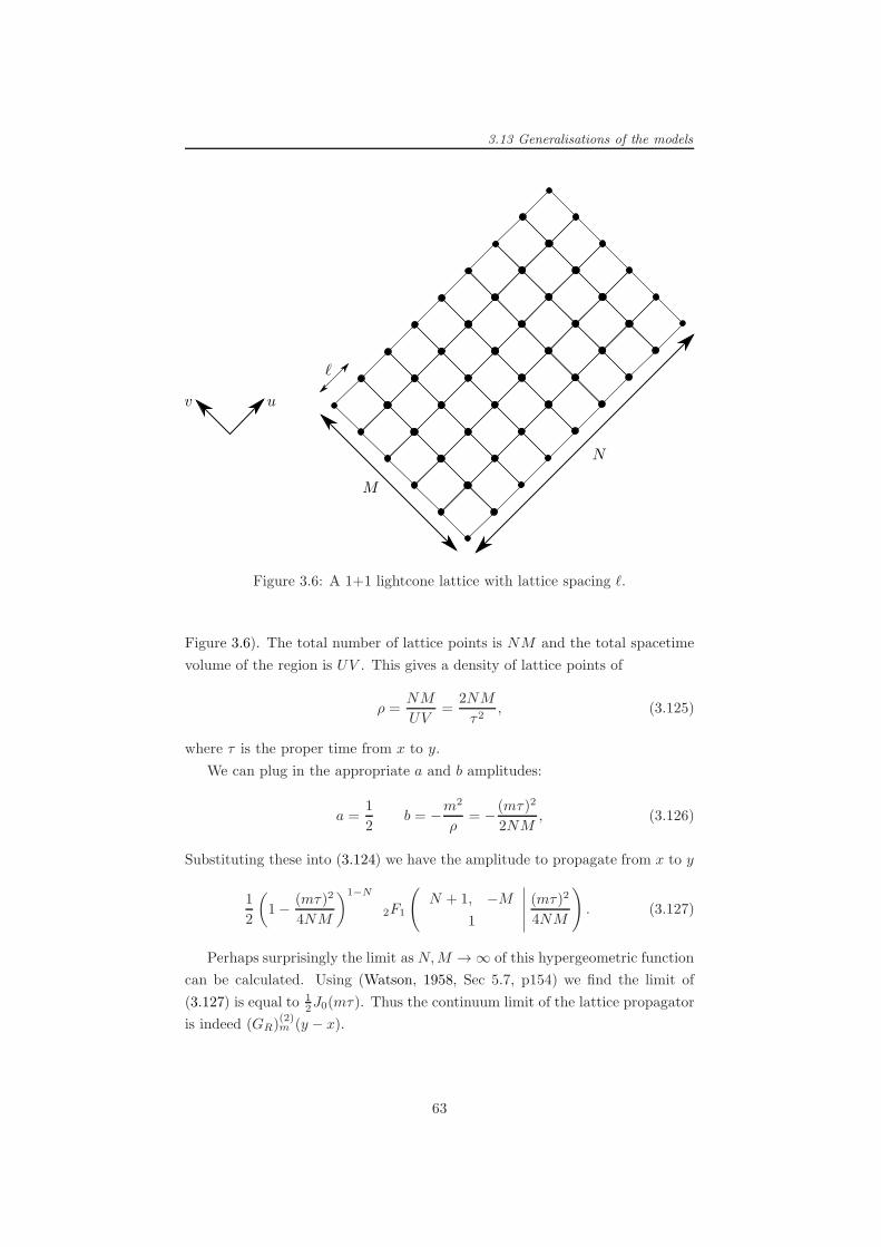
3.13 Generalisations of the models
Figure 3.6: A 1+1 lightcone lattice with lattice spacing ℓ.
Figure 3.6). The total number of lattice points is NM and the total spacetime
volume of the region is UV . This gives a density of lattice points of
ρ =NM
UV=
2NM
τ2, (3.125)
where τ is the proper time from x to y.
We can plug in the appropriate a and b amplitudes:
a =1
2b = −m
2
ρ= − (mτ)2
2NM, (3.126)
Substituting these into (3.124) we have the amplitude to propagate from x to y
1
2
(1− (mτ)2
4NM
)1−N
2F1
(N + 1, −M
1
∣∣∣∣∣(mτ)2
4NM
). (3.127)
Perhaps surprisingly the limit as N,M → ∞ of this hypergeometric function
can be calculated. Using (Watson, 1958, Sec 5.7, p154) we find the limit of
(3.127) is equal to 12J0(mτ). Thus the continuum limit of the lattice propagator
is indeed (GR)(2)m (y − x).
63
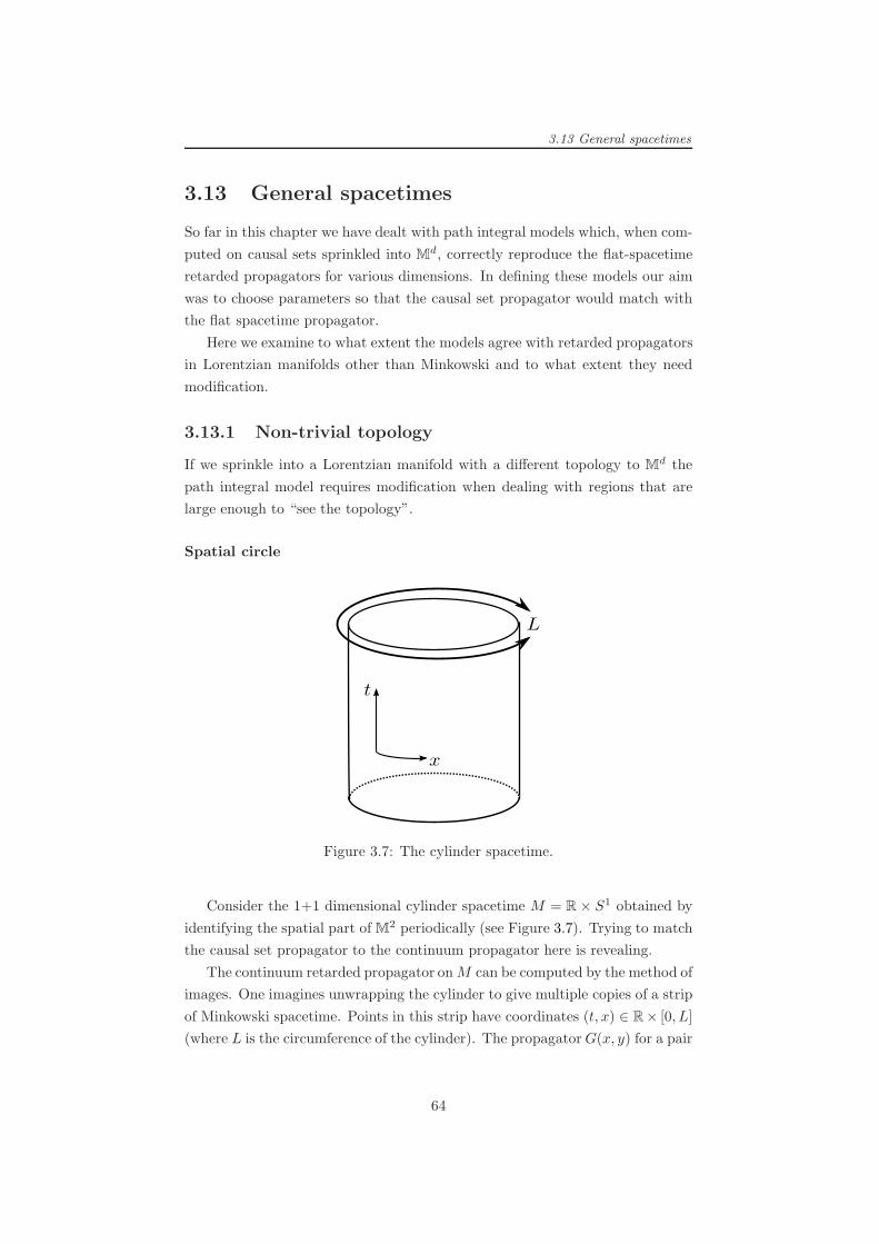
3.13 General spacetimes
3.13 General spacetimes
So far in this chapter we have dealt with path integral models which, when com-
puted on causal sets sprinkled into Md, correctly reproduce the flat-spacetime
retarded propagators for various dimensions. In defining these models our aim
was to choose parameters so that the causal set propagator would match with
the flat spacetime propagator.
Here we examine to what extent the models agree with retarded propagators
in Lorentzian manifolds other than Minkowski and to what extent they need
modification.
3.13.1 Non-trivial topology
If we sprinkle into a Lorentzian manifold with a different topology to Md the
path integral model requires modification when dealing with regions that are
large enough to “see the topology”.
Spatial circle
Figure 3.7: The cylinder spacetime.
Consider the 1+1 dimensional cylinder spacetime M = R× S1 obtained by
identifying the spatial part of M2 periodically (see Figure 3.7). Trying to match
the causal set propagator to the continuum propagator here is revealing.
The continuum retarded propagator onM can be computed by the method of
images. One imagines unwrapping the cylinder to give multiple copies of a strip
of Minkowski spacetime. Points in this strip have coordinates (t, x) ∈ R× [0, L]
(where L is the circumference of the cylinder). The propagatorG(x, y) for a pair
64

3.13 General spacetimes
of points x, y ∈ M is found by summing the Minkowski spacetime propagator
for the image points of x and y under the periodic identification.
Explicitly we have
G(x, y) =
∞∑
n=−∞(GR)
(2)m (y − x+ nv), (3.128)
where v = (0, L) is the vector that translates from one strip to the next. For
fixed x and y the contribution to G(x, y) actually involves only a finite sum
because (GR)(2)m (y − x+ nv) 6= 0 for only a finite number of n.
The massless case illustrates the issues involved most clearly. In Figure
3.8 we show the multiple copies of the unwrapped cylinder. For a fixed point
x ∈ M the values of the massless propagator G(x, y) are shown when y lies
within different regions in M .
In the causal set path integrals suitable for sprinklings into 2-dimensional
spacetimes the massless propagator is KR := 1/2C where C is the causal matrix
for the sprinkling. In Figure 3.9 we show, for the same point x, the expected
value of the causal set propagator for the same regions (i.e. the expected value
of 1/2C for sprinklings into M .)
If the region being sprinkled into does not wrap around the cylinder, i.e.
it’s too small to “see the topology”, then the expected value of the causal set
propagator equals the continuum propagator. However, for general regions on
the cylinder, it is clear from the figures that the expected value of the causal
set propagator does not equal the continuum propagator—the causal set path
integral does not take account of the cylinder topology.
The difficulty is that the causal relations only encode the spatial topology
implicitly. As an example, consider two causally related sprinkled points x, y ∈M . There may be a causal curve that goes from x to y without wrapping around
the cylinder. Then again, there may be a causal curve that wraps once around
(in either direction) or twice around etc. In short, there may be many classes
of causal curves from x to y, each distinguished by the number of times the
curves wrap around the cylinder (i.e. each class is a homotopy class of future-
directed causal curves15). When we sprinkle a causal set into M this wealth
of information (i.e. the number of times causal curves can wind around the
cylinder) is simply recorded as “x y”.
If we only focussed on the pair x and y then it appears the causal relations
cannot tell us this topological information. Nevertheless the causality theorems
discussed in Section 1.2.2 ensure that the causal relations do encode the topology
15See Geroch (1985, Chpt 34) for an introduction to homotopy. The massless G(x, y)is essentially just one half the number of homotopy classes of future-directed causal curvesjoining x and y.
65
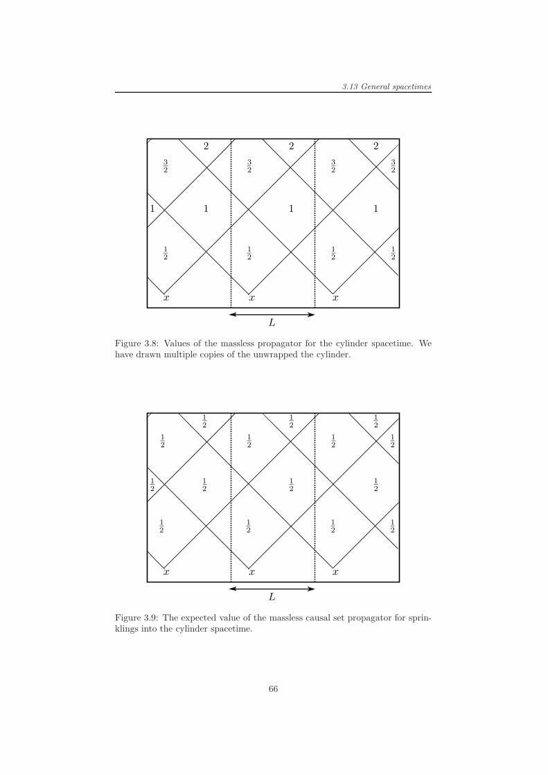
3.13 General spacetimes
Figure 3.8: Values of the massless propagator for the cylinder spacetime. Wehave drawn multiple copies of the unwrapped the cylinder.
Figure 3.9: The expected value of the massless causal set propagator for sprin-klings into the cylinder spacetime.
66
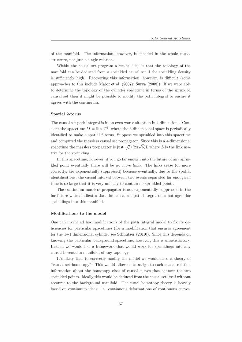
3.13 General spacetimes
of the manifold. The information, however, is encoded in the whole causal
structure, not just a single relation.
Within the causal set program a crucial idea is that the topology of the
manifold can be deduced from a sprinkled causal set if the sprinkling density
is sufficiently high. Recovering this information, however, is difficult (some
approaches to this include Major et al. (2007); Surya (2008)). If we were able
to determine the topology of the cylinder spacetime in terms of the sprinkled
causal set then it might be possible to modify the path integral to ensure it
agrees with the continuum.
Spatial 2-torus
The causal set path integral is in an even worse situation in 4 dimensions. Con-
sider the spacetime M = R× T 3, where the 3-dimensional space is periodically
identified to make a spatial 2-torus. Suppose we sprinkled into this spacetime
and computed the massless causal set propagator. Since this is a 4-dimensional
spacetime the massless propagator is just√ρ/(2π
√6)L where L is the link ma-
trix for the sprinkling.
In this spacetime, however, if you go far enough into the future of any sprin-
kled point eventually there will be no more links. The links cease (or more
correctly, are exponentially suppressed) because eventually, due to the spatial
identifications, the causal interval between two events separated far enough in
time is so large that it is very unlikely to contain no sprinkled points.
The continuum massless propagator is not exponentially suppressed in the
far future which indicates that the causal set path integral does not agree for
sprinklings into this manifold.
Modifications to the model
One can invent ad hoc modifications of the path integral model to fix its de-
ficiencies for particular spacetimes (for a modification that ensures agreement
for the 1+1 dimensional cylinder see Schmitzer (2010)). Since this depends on
knowing the particular background spacetime, however, this is unsatisfactory.
Instead we would like a framework that would work for sprinklings into any
causal Lorentzian manifold, of any topology.
It’s likely that to correctly modify the model we would need a theory of
“causal set homotopy”. This would allow us to assign to each causal relation
information about the homotopy class of causal curves that connect the two
sprinkled points. Ideally this would be deduced from the causal set itself without
recourse to the background manifold. The usual homotopy theory is heavily
based on continuum ideas: i.e. continuous deformations of continuous curves.
67

3.13 General spacetimes
It might be enough to find a suitable topology for “curves” (for example, chains
or paths) in the causal set such that continuous deformations can be defined.
3.13.2 Curved spacetimes
Perhaps the most interesting question is how well the causal set path integral
model extends to sprinklings into curved spacetimes. Now we briefly outline
the formalism for scalar field theory in general Lorentzian manifolds (we follow
Fulling (1989) and Birrell and Davies (1982, §3.2)).If (M, g) is a Lorentzian manifold then the generalisation of the Klein-Gordon
equation for a scalar field φ is (Fulling, 1989, eq 6.2, p117):
(+m2 + ζR(x))φ(x) = 0. (3.129)
Here ζ is a constant, R(x) is the Ricci curvature of the manifold and
φ =1√g∂µ[g
µν√g∂νφ], (3.130)
is the generalisation of the d’Alembertian to curved spacetimes (with g :=
| det(gµν)|).Green’s functions for this equation are distributionsG(x, y) satisfying (Fulling,
1989, p125):
(x +m2 + ζR(x))G(x, y) =δ(x − y)√
g. (3.131)
Solutions to this equation depend on the particular Lorentzian manifold that is
being used and calculating G(x, y) explicitly is very difficult for all but the sim-
plest cases. We note, however, that for any globally hyperbolic spacetime this
equation is guaranteed to possess unique retarded and advanced solutions (char-
acterised by their support properties in spacetime (Fulling, 1989, p79, p125)).
For sprinklings into a causal Lorentzian manifold the expectation value of
the causal set propagator, averaged over sprinklings, is a retarded function. It
is possible that for certain Lorentzian manifolds this function reproduces the
continuum retarded Green’s function.
One can investigate this by looking at simple examples. One of the simplest
are sprinklings into 1+1 dimensional Lorentzian manifolds. Such manifolds
are conformally flat so their causal relations can be calculated from the causal
relations in M2.
Another place where progress might be made is for sprinklings into space-
times with constant curvature: i.e. de Sitter or anti-de Sitter (for definitions
see Hawking and Ellis (1973, §5.2, p124)). Again these are conformally flat so
their causal relations can be computed using those of Md. In addition Meyer
68

3.14 Uses for the retarded propagator
(1988, Thm III.4, p68) gives expressions for the expected number of chains for
sprinklings into de Sitter and anti-de Sitter. While the expressions are compli-
cated it is possible that they could be used to find an exact expression for the
expected value of the sum-over-chains propagator in these spacetimes.
We mention that the path integral has the potential to be cope with position-
dependent curvature. This is because curvature of the background manifold
affects the distribution of sprinkled points. This in turn affects the distribution
of chains and paths in the causal set which then affects the combinatorics in the
sum over trajectories. It remains possible that without changing the hop and
stop amplitudes the model could correctly reproduce the curvature dependence
in the continuum Green’s functions.
Huygens Principle and Tails
One unusual phenomenon that occurs in curved spacetime is the presence of
tails. This is the name used when the Green’s function for the d’Alembertian
is non-zero for chronologically related points rather than just for null-related
points. In effect these non-zero “tail-terms” are due to “back-scattering” of
the field off the spacetime curvature. The absence of tails in the propaga-
tion of fields is one way to characterise Huygens’ principle: that radiation
should propagate only along the lightcone (Bombelli and Sonego (1994, p7182),
Sonego and Faraoni (1992)).
The massless propagator for sprinklings into 3+1 dimensional spacetimes is
proportional to the link matrix of the causal set. This means that in general
its expectation value will be strongly peaked on the lightcone and exponentially
small away from the lightcone. We see therefore that we don’t expect the causal
set propagator to reproduce a Green’s function with a tail-term. Physically
this says that massless particles propagate along the lightcone16, i.e. Huygens’
principle holds for the causal set model.
It thus seems that the 3+1 dimensional model would require modification if
it were to reproduce a Green’s function with a tail. Since these tails have not
been observed experimentally it is intriguing to speculate that the causal set
propagator might be the physically correct one!
3.14 Uses for the retarded propagator
We’ve concentrated so far on ways to derive the retarded propagator on a causal
set. In the next chapter we shall use this work to obtain a quantum scalar field
16or at least the causal set analogue of the lightcone.
69

3.14 Uses for the retarded propagator
theory and the Feynman propagator. For now we briefly mention some possible
uses that the retarded propagator could be put to on its own.
3.14.1 Yang-Feldman formalism
The Yang-Feldman formalism (Yang and Feldman, 1950) is an approach to
quantum field theory that uses the retarded and advanced propagators. Their
paper deals with quantum electrodynamics but the ideas apply to other theories.
We briefly outline the method applied to a self-interacting scalar field.
For such a theory the equation of motion is
( +m2)φ(x) = f(x), (3.132)
where φ is a field operator (acting on some Fock space) and f is an operator
representing an interaction (possibly depending on φ, e.g. f(x) = λφ3(x)). This
equation can be integrated using the retarded and advanced propagators to give
φ(x) = φin(x) +
∫ddy(GR)
(d)m (x− y)f(y), (3.133)
φ(x) = φout(x) +
∫ddy(GA)
(d)m (x− y)f(y), (3.134)
where φin and φout are solutions to the free field equation:
(+m2)φin(x) = (+m2)φout(x) = 0. (3.135)
The incoming (outgoing) field coincides with φ in far past (future) and represent
what the field would have been if the interaction was absent. Both the incoming
and outgoing fields satisfy the same free field commutation relations:
[φin(x), φin(x)] = [φout(x), φout(x)] = i∆(y − x), (3.136)
where ∆(x) := (GR)(d)m (x) − (GA)
(d)m (x) is the Pauli-Jordan function17. Since
the incoming and outgoing fields satisfy identical commutation relations they
must be related by a unitary transformation in the following way:
φout = S−1φinS. (3.137)
This unitary operator S defines the S-matrix for the theory.
To evaluate the matrix elements of the S operator the equations (3.133)
and (3.134) are solved iteratively by successive approximations. These approx-
17This will play a central role in the next chapter.
70

3.14 Uses for the retarded propagator
imations are then combined with (3.137) to compute the matrix elements to
a particular order (in a suitable coupling constant). This procedure is de-
scribed in general terms in Jauch and Rohrlich (1955, §8-7, p167). Apparently
this procedure is entirely equivalent to the usual Feynman diagram methods
(Jauch and Rohrlich, 1955, p169).
This approach gives a central role to the retarded and advanced propagators.
If we only have these propagators available on a causal set then perhaps they
could be used to define a causal set quantum field theory. In the next chapter,
however, we show how to define quantum field theory on a causal set in a simpler
manner.
3.14.2 Feynman tree theorem
In quantum field theory the Feynman propagator plays an important role. When
evaluating Feynman diagrams, for example, it is the Feynman propagator that is
associated to each leg of the diagram. It is interesting to wonder if a similar use
can be found for the retarded propagator which reproduces the same results—
can we reformulate quantum field theory using the retarded propagator?
A tantalising step in this direction is suggested in Feynman (2000) (also
available in Klauder (1972, p355-375)). There a method is described which
relates scattering amplitudes calculated with the Feynman propagator to scat-
tering amplitudes calculated with the retarded propagator.
The method relies on the fact that the Feynman propagator GF (x) and
retarded propagator GR(x) are related by
GF (x) = GR(x) +Gs(x), (3.138)
where Gs(x) is a solution to the Klein-Gordon equation.
By substituting this equation into the amplitude for a Feynman diagram
containing a closed loop we can re-express the amplitude as sums of “tree di-
agram” amplitudes (see Feynman (2000) for full details). These tree diagrams
contain no closed loops and it is the retarded propagator that is assigned to each
leg. A single loop diagram splits in this way into a sum over a number of dif-
ferent tree diagrams, each containing additional on-shell incoming and outgoing
particles. This result is known as the Feynman tree theorem.
In the paper it is subsequently claimed that the amplitude for complete
processes can be obtained by calculating with the retarded propagator only,
but making sure to include suitable additional on-shell particles—see Feynman
(2000, eq (22)′).
This method potentially offers a way to re-express quantum field theory
using only the retarded propagator. It requires, however, knowing how to sum
71

3.14 Uses for the retarded propagator
over incoming and outgoing particles which have definite on-shell momentum.
Carrying this over to define a field theory on a causal set might be possible but
requires the notion of on-shell momentum on a causal set (see Section 4.12 for
ideas in this direction).
3.14.3 Action-at-a-distance
It is possible to reformulate classical (and quantum) electrodynamics as a par-
ticle theory involving direct inter-particle interactions. In such a theory there
are no fields, only particles subject to certain relativistic interactions. Such a
reformulation is known as an “action-at-a-distance” theory.
Perhaps the best known such reformulation is the Wheeler-Feynman ab-
sorber theory (Wheeler and Feynman, 1945, 1949). This is a reformulation of
classical electrodynamics in which there is no radiation field. Instead the theory
describes the motion of charged particles subject to direct interactions. These
interactions are governed by both the retarded and advanced propagators. The
advanced effects, which are usually thought to lead to paradoxical “effect pre-
cedes cause” behaviour, turn out to cancel completely if the effect of the rest
of the universe is included. Matter elsewhere in the universe plays an essential
role as a giant absorber whose advanced effects are needed to ensure that the
theory appears to use only the retarded propagator.
The physical picture in this theory is very different to the usual electrody-
namics but, perhaps surprisingly, it is possible to show that the theory repro-
duces the same results as conventional electrodynamics.
Given that such a familiar theory as classical electrodynamics can be so rad-
ically reformulated yet still reproduce the same physical results, it is interesting
to speculate on whether a reformulation of standard physical theories (in such
action-at-a-distance terms) could help when trying to define them on a causal
set. Certainly the non-locality of a causal set (in which each element is linked to
a large number of other elements) fits more closely with an action-at-a-distance
formulation rather than a local differential description.
One attempt to formulate action-at-a-distance electrodynamics on a discrete
spacetime was given in Hemion (1988). There he formulates a theory of particles
which exist within a locally finite partially ordered set. By identifying analogues
of proper distances in the discrete spacetime he aims to assign an action to par-
ticle configurations. The hope is that by extremising this action it is possible to
identify the dynamically allowed particle configurations. Unfortunately the con-
tinuum action depends on the velocities of particles and Hemion side-steps the
difficulties present in defining such velocities on a discrete spacetime (Hemion,
1988, p1193).
72

3.14 Uses for the retarded propagator
The action-at-a-distance formulation of physics has also been advocated by
Hoyle and Narlikar (1974). In this set of lectures they discuss reformulating
quantum electrodynamics as an action-at-a-distance theory. Interestingly in
their Section 8.1 they discuss mass scatterings very similar to those in our
Section 3.9. They discuss a path integral in which the particle can, in our
language, “hop” into the future or past lightcone at each step (i.e they use half
the sum of the retarded and advanced massless propagators as their massless
propagator).
It is them emphasised that, since such zig-zag paths can stray arbitrarily far
from the initial or final points, to assign them the correct amplitude we must
know how the “mass field” m behaves everywhere in the universe (p144). If we
allow ignorance of this behaviour and restrict the path integral to a finite region
then, they claim, we can derive the Feynman propagator as the sum of the free
particle propagator plus the “response of the universe” (p144-145). If this is
correct then it presents an intriguing way to derive the Feynman propagator
from the retarded and advanced propagators.
It’s possible that action-at-a-distance ideas could lead to a new way to define
physical theories on a causal set. Unfortunately in theories of this type the
analysis of even a small-scale physical system requires that the behaviour of the
entire universe be included. To implement this on a causal set it seems clear
that knowledge of the entire causal set is needed, as well as a way to “screen
out” the background behaviour of the rest of the universe. While this sounds
like a formidable task it’s possible that future developments could lead in this
direction.
73

Chapter 4
Free Quantum Field Theory
I had asked Salam “what IS a quantised field”, and received the
answer “Good; I was afraid you would ask me something I did not
know. A quantised field, phi(x) at the point x of space-time, is that
operator assigned by the physicist using the correspondence princi-
ple, to the classical field phi at the point x”. I went away thinking
about this; then I realised that what I needed was a statement of
WHICH operator is assigned by the physicist.
Ray Streater, 1957, in Streater (2000).
4.1 Motivation
The best theory to describe matter at a fundamental level is currently quantum
field theory. This theoretical framework grew out of efforts to combine quantum
mechanics with special relativity in the 1920s-1940s. The most successful quan-
tum field theory is the Standard Model which was developed in the 1960s-1970s.
This successfully describes the electromagnetic, weak and strong fundamental
forces. Despite the physical successes of the quantum field theory framework its
mathematical underpinnings have remained poorly-defined.
One of the major obstacles to a mathematically well-defined quantum field
theory is the presence of divergences. These are typically divergent integrals or
sums which must be regularised before finite answers can be calculated. The
removal of the divergences presented a serious obstacle in the development of
the theoretical framework. In the 1940s renormalisation techniques were de-
veloped which avoided the divergences and enabled finite answers for physical
predictions to be obtained. These predictions matched experiments very well
74

4.2 Motivation
and renormalisable quantum field theories became established as a central part
of modern physics.
The modern perspective on renormalisation is that quantum field theories
provide only an effective description of matter. The idea is that we simply do not
know the precise theory of physics at very small length scales (or equivalently
very high energies). If we admit our ignorance about this and “integrate out”
the small-scale behaviour of the theory we are left with an effective description
that gives us the correct answer at the length-scales we’re probing.
An alternative approach is to try to formulate a model for matter which
avoids the divergences from the beginning. This is one of the motivations for
considering discrete spacetime and is the approach we are aiming at.
4.1.1 Discrete spacetime and field theory
An obvious way to try to curb the divergences is to discretise spacetime. The
most direct way, and one that it frequently used, is to ignore relativistic invari-
ance and simply replace the continuum spacetime with a hyper-cubic lattice.
One early approach along these lines was the 1930 suggestion by Heisen-
berg that the world is a “lattice world”—a Gitterwelt. In this sketch of an
idea the differential equations of physics were to be replaced by finite-difference
equations. By this route it was hoped that the divergences could be avoided.
Discrete spacetime also appears in a more pragmatic, less foundational ap-
proach known as lattice field theory. Since the continuum theory is difficult to
solve analytically one can try to numerically solve the equations iteratively on
a computer. To make the problem well-posed for numerical simulations this
usually involves Wick rotating the theory to Euclidean space and then laying
down a hyper-cubic lattice. This approach is particularly used for strongly-
interacting quantum field theory where the usual perturbative expansion is not
useful. Nevertheless the use of a Wick rotation and a hyper-cubic lattice mean
the lattice that is used shares few of the properties of physical spacetime (e.g.
spacetime’s Lorentzian signature and Lorentz-invariance).
4.1.2 Causal set field models
Quantum field theory on a causal set has been previously considered by a number
of people. There are two main approaches to the problem—modelling matter
as the causal set or modelling matter on the causal set.
75

4.2 Scalar fields as geometry
4.2 Scalar fields as geometry
One approach to modelling fields on a causal set follows the spirit of Wheeler’s
geometrodynamics in which matter and spacetime are unified—indeed matter is
spacetime. Inspired by this approach one can imagine that individual particles
or field configurations are really particular patterns of causal relations or clusters
of causal set elements which propagate (or perhaps, repeat) through the causal
set.
We mention a few ways in which the causal set itself could be used to encode
a matter field (methods 1 and 2 have been considered by David Rideout).
4.2.1 Method 1
For a causal set (C,) we define an equivalence relation u ∼ v if u, v ∈ C share
identical (strict) causal relations (i.e. u and v are a “non-Hegelian pair”):
u ∼ v if, for all w,w′ ∈ C, we have w ≺ u ≺ w′ ⇐⇒ w ≺ v ≺ w′. (4.1)
Each equivalence class under ∼ is an antichain of some cardinality (which may
be equal to one). We can create a new causal set (C′,′) by starting with the
set of equivalence classes: C′ := [u] : u ∈ C. This set inherits an order relation
from C in a natural way:
u v =⇒ [u] ′ [v], (4.2)
for all u, v ∈ C.Our original causal set (C,) is equivalent to the new causal set (C′,′) if
every element of C′ is assigned a natural number equal to the cardinality of the
equivalence class (see Figure 4.1).
In this way we can encode a positive integer-valued scalar field in terms of
the causal set itself.
4.2.2 Method 2
Another approach involves dropping the requirement that is antisymmetric.
This leaves us with a preposet (or quasi-ordered set) (C,) in which is reflexive
and transitive (Stanley, 1986, p153, Ex. 1a). If is not antisymmetric then
causal loops are allowed—these are n distinct elements related as: v1 ≺ v2 ≺. . . vn−1 ≺ vn ≺ v1.
We can define an equivalence relation u ∼ v if u, v ∈ C are in the same causal
loop:
u ∼ v if u v and v u. (4.3)
76
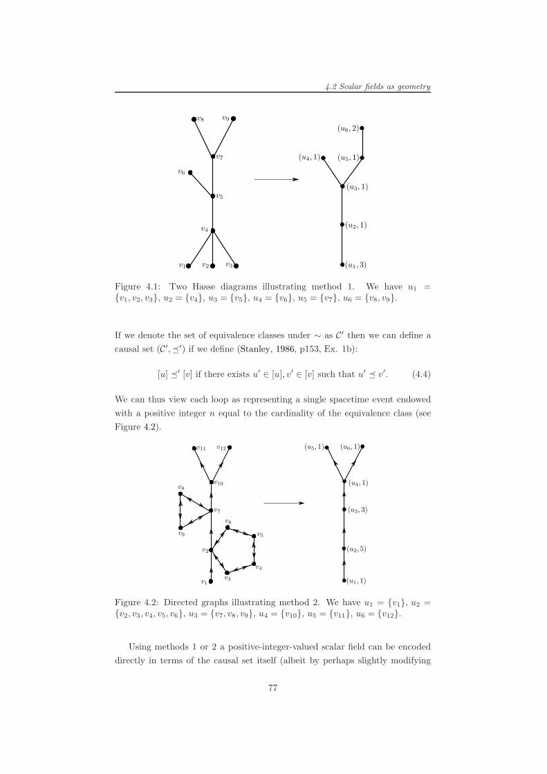
4.2 Scalar fields as geometry
Figure 4.1: Two Hasse diagrams illustrating method 1. We have u1 =v1, v2, v3, u2 = v4, u3 = v5, u4 = v6, u5 = v7, u6 = v8, v9.
If we denote the set of equivalence classes under ∼ as C′ then we can define a
causal set (C′,′) if we define (Stanley, 1986, p153, Ex. 1b):
[u] ′ [v] if there exists u′ ∈ [u], v′ ∈ [v] such that u′ v′. (4.4)
We can thus view each loop as representing a single spacetime event endowed
with a positive integer n equal to the cardinality of the equivalence class (see
Figure 4.2).
Figure 4.2: Directed graphs illustrating method 2. We have u1 = v1, u2 =v2, v3, v4, v5, v6, u3 = v7, v8, v9, u4 = v10, u5 = v11, u6 = v12.
Using methods 1 or 2 a positive-integer-valued scalar field can be encoded
directly in terms of the causal set itself (albeit by perhaps slightly modifying
77

4.3 Scalar fields on a causal set
the definition of a causal set in method 2).
4.2.3 Kaluza-Klein theory on a causal set
Another approach to modelling matter on a causal set is to attempt to define
Kaluza-Klein theory on a causal set1. In standard continuum Kaluza-Klein
theory the dynamics of pure gravity in a higher dimensional Lorentzian mani-
fold give rise to coupled gravity-matter fields in a lower dimensional Lorentzian
manifold.
To implement this idea for causal set theory one could imagine sprinkling
into M4 × S where S is some compact Riemannian manifold (e.g. a circle or
torus). One could then write down the gravitation dynamics for this causal set
(e.g. the Einstein-Hilbert causal set action discussed in Section 2.3.3). The idea
is that this expression would split easily into two parts: (i) the 4-dimensional
causal set action and (ii) an action for matter fields. By correctly identifying the
action for matter fields it may be possible to define suitable quantities intrinsic
to the causal set to serve as the matter fields themselves. So far, however, this
remains only a sketch of an idea.
4.3 Scalar fields on a causal set
An alternative to modelling matter as the causal set itself is to model matter on
the causal set. This approach is similar to the usual theories of matter described
on a background Lorentzian manifold.
4.3.1 The d’Alembertian
A free classical scalar field on a Lorentzian manifold satisfies the Klein-Gordon
equation. A natural step towards defining field theory on a causal set is to
somehow discretise this equation. This involves finding a causal set analogue of
the d’Alembertian differential operator.
There have been two main approaches to this problem. Both of them aim
to find an expression intrinsic to the causal set that plays the role of the
d’Alembertian operator.
Once we have such an expression we can check its validity as follows. Fix
a finite region R ⊂ Md with a real scalar field φ : R → R defined on it. Fix a
point x ∈ R. If we sprinkle a causal set into R there is zero probability that x
will be a sprinkled point. We therefore add x to the sprinkled causal set (and
label it as element v1, say). The generated causal set inherits the scalar field
1This was suggested to the author by Sumati Surya.
78
4.3 Scalar fields on a causal set
from R by assigning the value of φ at each sprinkled point as the value of the
causal set scalar field.
We can now apply the causal set d’Alembertian to the causal set field to
obtain the d’Alembertian of the field at the element v1 (i.e. the element cor-
responding to the point x ∈ R). By averaging this value over all sprinklings
into R (with the same density) we obtain the expected value of the causal set
d’Alembertian of φ at x. We can compare this to φ(x) to see if the causal set
expression gives the right answer.
Method 1: Inverting the Green’s function
The first attempt to obtain the d’Alembertian on a causal set was pursued by
Daughton (1993) and later by Salgado (2008). They start with the continuum
equation satisfied by a Green’s function G(x) for the d’Alembertian in Md:
G(x) = δd(x). (4.5)
The idea is that on a finite p-element causal set this equation should be replaced
by a matrix equation:
BG = I, (4.6)
where B and G are now p× p matrices and I is the identity matrix2. B is the
candidate d’Alembertian operator and G is a causal set analogue of a continuum
Green’s function.
As we have seen in the previous chapter it is possible to obtain causal set
analogues for the retarded (and advanced) d’Alembertian Green’s functions for
sprinklings into Md for d = 1, 2, 3, 4. The idea is to invert these matrices to
obtain a candidate for the d’Alembertian operator: B := G−1.
Unfortunately the matrix for the retarded Green’s function KR is non–
invertible (we can see this because KR is zero on the diagonal and a labelling
can be chosen to ensure it is strictly upper triangular). Two options have been
explored to side-step this difficulty. Firstly one can include a non-zero diago-
nal value for the retarded propagator (in which case the matrix is guaranteed
to be invertible). Secondly one can work with the symmetric half-advanced,
half-retarded Green’s function equal to (KR +KA)/2 = (KR +KTR)/2 (which,
depending on the causal set, may or may not be invertible).
For sprinklings into M2, for example, KR = 1/2C (where C is the causal
2Strictly speaking, on dimensional grounds, the identity matrix should be multiplied by afactor of 1/V0 where V0 is the dimensionful fundamental volume assigned to the causal setelements. This is to ensure that the causal set equation has the same mass-dimension as thecontinuum equation it seeks to emulate. In Daughton (1993) and Salgado (2008) this issue isignored as they set V0 = 1.
79
4.3 Scalar fields on a causal set
matrix for the causal set) and the two candidate d’Alembertians are either
B =
(cI +
1
2C
)−1
, (4.7)
for some constant c (usually take to be 1/2) or
B =
(1
4(C + CT )
)−1
. (4.8)
Both Daughton and Salgado have performed extensive numerical simula-
tions which attempt to check the validity of these d’Alembertian operators for
sprinklings into M2. Their results suggest that the expected value of the causal
set d’Alembertian is a good approximation to the continuum d’Alembertian for
fields which vary slowly on the discreteness scale and are zero on the boundary
of the sprinkled region.
Method 2: Summing over layers
A second approach to the d’Alembertian has been pursued by Sorkin (2007,
2009); Benincasa and Dowker (2010). Here the approach is more direct and
starts with an attempt to finite-difference the d’Alembertian differential opera-
tor. The requirement that this be done in a Lorentz-invariant way leads to the
idea that the d’Alembertian of a field at an element vx in the causal set should
be a sum over the values of the field on “layers” of causal set elements to the
past of vx.
These layers are defined in terms of the cardinality of the inclusive causal
interval between an element and vx. Layer n is the set of all elements u such
that |[u, vx]| = n+ 1. So, for example, the first layer is the set of all past links
of vx.
The d’Alembertian of the field at vx is then a sum of the field values over
different layers, each layer weighted by a suitable coefficient. By looking at the
expected value of such expressions it is possible to choose combinations of layers
such that the causal set d’Alembertian is equal to the continuum d’Alembertian
in the infinite sprinkling density limit. This method has a surprising connec-
tion with the retarded propagators derived in the previous chapter (see Section
A.3.2).
Unfortunately the fluctuations of the causal set d’Alembertian are large and
grow with the sprinkling density. One way around this is to introduce a meso-
scale which lies somewhere between the discreteness scale and the nuclear scale.
The layers being summed over are then fattened out to the size of the meso-
scale and in this way the fluctuations are dampened down (see Sorkin (2007)
80

4.4 Quantum scalar field theory in Minkowski spacetime
for details).
It remains to be seen how these d’Alembertians expressions can be used to
define a field theory on a causal set.
4.3.2 Field actions
An alternative approach to defining scalar fields on a causal set has been pursued
by Sverdlov and Bombelli (2009a,b). This approach starts with a classical field
defined on a Lorentzian manifold. The Lagrangian for such a field is them re-
expressed in terms of the causal structure, the volume element and the proper
time, all of which have causal set analogs.
This expression can be simply discretised by making the appropriate substi-
tutions. In this way it’s possible to define a Lagrangian for a scalar field on the
causal set. The resulting expressions, however, are very complicated and one
has to work hard to ensure they don’t pick out a particular reference frame.
Further work along these lines has been pursued by Sverdlov (2008a,b,c,
2009). The same method, of re-expressing continuum quantities and then dis-
cretising, is applied to gauge fields and spinor fields. This top-down approach,
which starts with continuum quantities and then finds a suitable discretisation
is a good first-step but leads to causal set expressions that are complicated and
somewhat artificial. An approach which instead starts with a theory defined on
a causal set and then shows that it reproduces the continuum theory is more
appealing.
4.4 Quantum scalar field theory in Minkowski
spacetime
Before describing the model for free scalar quantum field theory on a causal set
we first review scalar quantum field theory in d-dimensional Minkowski space-
time Md.
4.4.1 Feynman propagator
In Section 3.3 the retarded, (GR)(d)m (x), and advanced, (GA)
(d)m (x), propagators
for the Klein-Gordon in spacetimes of dimension d = 1, 2, 3, 4 were given.
Here we describe another propagator for the Klein-Gordon equation—the
81

4.4 Quantum scalar field theory in Minkowski spacetime
Feynman propagator3. This is a Green’s function for the Klein-Gordon equation:
(+m2)(GF )(d)m (x) = δd(x), (4.9)
but with a different boundary condition. This boundary condition is usually
described in terms of the way positive and negative frequency modes are propa-
gated but here, instead, we shall simply use the usual Fourier transform contour
prescription to define:
(GF )(d)m (x) := lim
ǫ→0+− 1
(2π)d
∫ddp
e−ipx
p2 −m2 + iǫ. (4.10)
As with the retarded and advanced propagators a rigorous treatment of this
relies on the theory of distributions. This can be done in different dimensions
(Gel’fand and Shilov (1964, §2.8, p287) evaluate this Fourier transform explic-
itly). In Birrell and Davies (1982, eq 2.77, p23) it is stated that the general
form of (GF )(d)m in d-dimensions is given by4
(GF )(d)m (x) = lim
ǫ→0+
π
2
(−1)d
(2π)d/2
(m√τ2 − iǫ
)d/2−1
H(2)d/2−1
(m√τ2 − iǫ
). (4.11)
This agrees with the expression given in Gel’fand and Shilov (1964, eq 9, p289)
when appropriate factors of i, 2π etc are taken into account.
The ǫ→ 0 limit must be taken within the framework of distribution theory.
In the d = 4 case, for example, a delta-function term is present which is not
readily apparent unless care is taken with the limit. The Feynman propagator
can be expressed in d = 1, 2, 3, 4 dimensions as5:
(GF )(1)m (x) = −exp(−ims)
2im(4.12)
(GF )(2)m (x) =
1
4H
(2)0 (ms) (4.13)
(GF )(3)m (x) =
−i4π
exp(−ims)s
(4.14)
(GF )(4)m (x) =
1
4πδ(s2)− m
8π
H(2)1 (ms)
s(4.15)
where s =√(x0)2 − ~x2 for (x0)2 ≥ ~x2 and s = −i
√~x2 − (x0)2 for (x0)2 < ~x2.
3This is also known as the causal propagator. It is somewhat mis-named, apparently havingbeen first introduced by Stueckelberg and Rivier (Bogoliubov and Shirkov, 1959, Footnote 30,p141).
4We have replaced their n by d, their σ by 12τ2, multiplied their equation by −1 and
rearranged factors of 2 and i etc.5The d = 1 expression can be calculated directly. The d = 2 and d = 3 expressions
appear in Zhang et al. (2008, eqs 13 and 16). The d = 4 expression is derived in detail inBogoliubov and Shirkov (1959, §15, p 147) and De Jager, E.M. (1967).
82

4.5 Quantum scalar field theory in Minkowski spacetime
Note that s = limǫ→0+√τ2 − iǫ. H
(2)α is a Hankel function of the second kind
of order α and δ(s2) is the Dirac delta-function.
We note that, from the definition of GF , its real part is given by:
ℜ[(GF )(d)m (x)] =
(GR)(d)m (x) + (GA)
(d)m (x)
2. (4.16)
We also note that the in d = 2 case the massless limit of the imaginary part
of the Feynman propagator diverges (i.e. the massless limit of (GF )(2)m does not
exist).
4.4.2 Quantum fields
A free real bosonic scalar field is represented by an algebra of field operators
φ(x) (which act on a Fock space F ) satisfying the following conditions:
1. (+m2)φ(x) = 0, (4.17)
2. φ(x) = φ(x)†, (4.18)
3. [φ(x), φ(y)] = i∆(y − x), (4.19)
Here [A, B] := AB − BA is the commutator of two operators and ∆(x) is the
Pauli-Jordan function (or commutator function) defined as the difference be-
tween the retarded and advanced propagators (Bogoliubov and Shirkov, 1959):
∆(x) := GR(x)−GA(x). (4.20)
In addition there exists a Poincare invariant vacuum state |0〉 ∈ F . With the
fields so defined the Feynman propagator is given by the vacuum expectation
value of the time-ordered product of two field operators:
GF (y − x) = i〈0|T φ(x)φ(y)|0〉. (4.21)
The time-ordering has time increasing from right to left. The vacuum expecta-
tion value 〈0|φ(x)φ(y)|0〉 (without time-ordering) is called the two-point function
(or Wightman function).
We note that applying (x +m2) to the commutator in (4.19) gives
[(x +m2)φ(x), φ(y)] = (x +m2)i∆(y − x) = 0. (4.22)
That is, even if only (4.18) and (4.19) hold, we have that (x +m2)φ(x) com-
mutes with all the φ(y)6.
6This was emphasised to the author by Johan Noldus.
83

4.5 Quantum scalar field theory on a causal set
4.5 Quantum scalar field theory on a causal set
Our aim now is to define scalar quantum field theory on a causal set. In par-
ticular we are interested in defining a candidate Feynman propagator on the
causal set. These results appear in Johnston (2009a).
4.5.1 The Pauli-Jordan function
The starting point for our model is the causal set analogue of the Pauli-Jordan
function.
Let (C,) be a finite causal set with p elements generated by a sprinkling
into a finite causal interval A ⊂ Md. Using the results of the previous chapter we
define a p×pmatrixKR as the appropriate definition of the retarded propagator.
It then follows that the transpose of this matrix KA := KTR is the appropriate
definition of the advanced propagator. The real skew-symmetric matrix defined
by
∆ := KR −KA, (4.23)
is then the causal set analogue of the Pauli-Jordan function (compare with
(4.20)).
The matrix i∆ is skew-symmetric7 and Hermitian8. These two properties
ensure its rank9 is even (Perlis, 1958) and its non-zero eigenvalues appear in real
positive and negative pairs. We label its eigenvalues and normalised eigenvectors
as follows:
i∆ui = λiui, i∆vi = −λivi, i∆wk = 0, (4.24)
where λi > 0, 2s is the rank of i∆ and i = 1, . . . , s; k = 1, . . . , p− 2s.
These eigenvectors form an orthonormal basis for Cp and can be chosen such
that
ui = v∗i , wk = w∗k, (4.25)
u†iuj = v†i vj = δij , w†kwl = δkl, u†ivj = w†
kui = w†kvi = 0, (4.26)
for all i, j = 1, . . . , s; k, l = 1, . . . , p− 2s (where z∗ denotes complex conjugate
of z and u† := (u∗)T is the Hermitian conjugate of a column vector u).
In terms of these eigenvectors the Pauli-Jordan function is given by
i∆ =
s∑
i=1
λiuiu†i −
s∑
i=1
λiviv†i . (4.27)
7A matrix Mxy is skew-symmetric if Mxy = −Myx, i.e. MT = −M .8The Hermitian conjugate of a matrix Mxy is the matrix (M†)xy := M∗
yx. A matrix is
Hermitian if M = M†.9The rank of a matrix is the number of non-zero eigenvalues it possesses.
84

4.5 Quantum scalar field theory on a causal set
The Q matrix
It’s useful to define the Hermitian, positive semi-definite10 p× p matrix
Q :=
s∑
i=1
λiuiu†i , (4.28)
such that i∆ = Q − Q∗ = Q − QT . This Q is obtained from i∆ by restricting
i∆ to its “positive eigenspace” (i.e. the subspace spanned by eigenvectors with
positive eigenvalues). This matrix will turn out to play the role of the two-point
function in the causal set quantum field theory.
We can express Q in another way using the eigen-decomposition of i∆. Since
i∆ is Hermitian there exists a unitary matrix U (whose columns are the eigenvec-
tors of i∆) and a diagonal matrix D (whose diagonal entries are the eigenvalues
of i∆) such that
i∆ = UDU †. (4.29)
If we define two diagonal matrices containing the positive and negative eigen-
values:
(D+)xy :=
Dxy if Dxy > 0
0 otherwise(D−)xy :=
Dxy if Dxy < 0
0 otherwise(4.30)
such that D = D+ + D− then we have Q = U(D+)U †. In practice this is a
simple way to compute Q on a computer.
Another way to characterise Q is as
Q =1
2
(√(i∆)2 + i∆
). (4.31)
The matrix (i∆)2 is positive semi-definite and, as such, possesses a unique
positive semi-definite square root (Simon and Reed, 1972, Thm VI.9). It is this
matrix that we denote by√(i∆)2. It follows from Q − Q∗ = i∆ that the
imaginary part of Q is ℑ[Q] = ∆/2. Combining this with (4.31), we have
ℜ[Q] =
√(i∆)2
2, ℑ[Q] =
∆
2. (4.32)
Yet another way to characterise the Q matrix is as the unique Hermitian
positive semi-definite matrix that is closest to i∆ as measured in the Frobenius
norm (Dorf, 1997, p324).
10A p×p matrixMxy is positive semi-definite if it is Hermitian and z†Mz ≥ 0 for all z ∈ Cp.
85

4.5 Quantum scalar field theory on a causal set
4.5.2 Fields on a causal set
To model a free real scalar field on the causal set (C,) we suppose that to
every element vx ∈ C we assign a field operator φx (which acts on some Hilbert
space H). These field operators are then defined to satisfy the following three
conditions:
1. φx = φ†x, (4.33)
2. [φx, φy] = i∆xy, (4.34)
3. i∆w = 0 =⇒p∑
x′=1
wx′ φx′ = 0, (4.35)
for x, y = 1, . . . , p. In condition 3 w is a p-component column vector of complex
numbers. The first two conditions are natural generalisations of the continuum
case (compare (4.18) and (4.17)). Condition 3 ensures that any linear combina-
tion of field operators that commutes with all the field operators must be zero.
By (4.22) this is the analogue of imposing the Klein-Gordon equation on the
field operators (for further discussion of this point, see Section 4.5.3).
From these field operators we can define new operators11
ai :=
p∑
x=1
1√λi
(vi)xφx, a†i :=
p∑
x=1
1√λi
(ui)xφx. (4.36)
for i = 1, . . . , s. They satisfy (a†i )† = ai and
[ai, aj ] =vTi i∆vj√λiλj
=−λju†ivj√
λiλj= 0, (4.37)
[a†i , a†j ] =
uTi i∆uj√λiλj
=λjv
†iuj√λiλj
= 0, (4.38)
[ai, a†j ] =
vTi i∆uj√λiλj
=λju
†iuj√λiλj
= δij . (4.39)
which are readily recognised as the commutation relations for s creation opera-
tors (the a†i ) and s annihilation operators (the ai).
The transformation from the φx operators to the ai and a†i operators can be
inverted to give
φx =
s∑
i=1
√λi(ui)xai +
√λi(vi)xa
†i , (4.40)
(here we use the orthogonality of the eigenvectors (4.26) as well as (4.35)).
We now define a vacuum state vector |0〉 ∈ H by the conditions that ai|0〉 = 0
11These are normalised differently to the operators appearing in Johnston (2009a).
86

4.5 Quantum scalar field theory on a causal set
for all i = 1, . . . , s and 〈0|0〉 = 1. This allows us to recognise that H is the Fock
space spanned by basis vectors (a†1)n1(a†2)
n2 · · · (a†s)ns |0〉 for integers ni ≥ 0,
i = 1, . . . , s.
4.5.3 Uniqueness and condition 3
As we have just shown, any algebra of causal set field operators φx that satisfies
the three conditions:
1. φx = φ†x, (4.33)
2. [φx, φy] = i∆xy, (4.34)
3. i∆w = 0 =⇒p∑
x′=1
wx′ φx′ = 0, (4.35)
can be expressed in the form:
φx =s∑
i=1
√λi(ui)xai +
√λi(vi)xa
†i , (4.40)
This means we have found one way to represent the φx operators (namely
as operators on the Fock space associated to the ai and a†i operators. Further
details of this Fock space will be given in Section 5.2). A natural question is
whether this representation of the φx operators is unique—do there exist other
ways of representing the field operators that are essentially different to this
representation?
Through (4.40) the uniqueness of the φx operators is equivalent to the
uniqueness of the ai and a†i operators satisfying the commutation relations
(4.37), (4.38), (4.39). The Stone-von Neumann theorem (Bratteli and Robinson,
1981, Cor 5.2.15, p34) ensures that these commutation relations possess a unique
(up to unitary equivalence) representation as operators on a Fock space. This
means that any other collection of 2s operators satisfying the same commutation
relations is related to the ai and a†i by a unitary transformation.
A crucial part of this theorem is the fact that there are a finite number of
ai and a†i operators. If there are an infinite number (i.e. if i ranged from 1 to
infinity) then there exist unitarily inequivalent representations. It is therefore
interesting to wonder what modifications may be necessary to extend the field
operator model to infinite causal sets (see Section 4.8.2).
87
4.5 Quantum scalar field theory on a causal set
Condition 3
Of the three conditions the first two are natural analogues of the continuum
conditions for field operators. It is the third:
i∆w = 0 =⇒p∑
x′=1
wx′ φx′ = 0, (4.35)
however, that appears the most ad hoc. It is motivated by the fact that in the
continuum (+m2)φ(x) commutes with all the φ(y) operators (see (4.22)). In
the causal set model we have, from (4.34),
i∆w = 0 =⇒[
p∑
x′=1
wx′ φx′ , φy
]= (wT i∆)y = 0. (4.41)
Imposing condition 3 therefore ensures that any linear combination of the φx
that commutes with all the φy should be set to zero. This is similar to setting
(+m2)φ(x) = 0 in the continuum.
The effect of condition 3 is to make the algebra of field operators as small as
possible, so long as it’s consistent with conditions 1 and 2. If we had not imposed
condition 3 then the most general expression for the φx operators (which satisfy
conditions 1 and 2) would be:
φx =
s∑
i=1
√λi(ui)xai +
√λi(vi)xa
†i +
p−2s∑
k=1
(wk)xck, (4.42)
where the wk are the p− 2s linearly independent real eigenvectors of i∆ with 0
eigenvalue: i∆wk = 0. If all we know is that the φx operators satisfy conditions
1 and 2 then the ck are arbitrary but satisfy
ck =
p∑
x=1
(wk)xφx, (4.43)
and have the following commutation relations:
[ck, ai] = [ck, a†i ] = 0, [ck, cl] = 0, (4.44)
for i = 1, . . . , s and k, l = 1, . . . , p − 2s. Imposing condition 3 is equivalent to
imposing that ck := 0 for all k. Without this condition we would need to specify
what the ck operators were if we wanted to completely define the φx operators.
Thus condition 3 ensures that the φx operators only depend on the ai and a†i
operators.
As it turns out, condition 3 also enforces some desirable properties in the
88
4.6 Feynman propagator on a causal set
operator algebra. Suppose vx, vy ∈ C are a non-Hegelian pair of causal set
elements (meaning they share identical strict causal relations). Condition 3
ensures that the field operators assigned to these elements are equal: φx = φy.
We can see this because the x and y rows and columns in i∆ are identical
(because vx and vy share identical strict causal relations). This means that the
p-component vector w = ~ex − ~ey (where the ~ei are the standard basis vectors
only non-zero in the ith position) satisfies i∆w = 0. Applying condition 3 to this
implies φx − φy = 0 or φx = φy. The same argument applies to any collection
of non-Hegelian elements. This is pleasing because non-Hegelian elements are
identical as far as the causal set is concerned so it is sensible that they are
assigned identical field operators.
In addition, if vx ∈ C is a single element, unrelated to all others, then φx = 0.
This is because the xth row and column in i∆ is equal to zero which ensures
that w = ~ex satisfies i∆w = 0. Applying condition 3 ensures φx = 0.
4.6 Feynman propagator on a causal set
Directly from the equation
φx =
s∑
i=1
√λi(ui)xai +
√λi(vi)xa
†i , (4.40)
the two-point function can be evaluated as
〈0|φxφy |0〉 =s∑
i=1
s∑
j=1
√λiλj(ui)x(vj)y〈0|aia†j |0〉 (4.45)
=s∑
i=1
s∑
j=1
√λiλj(ui)x(vj)yδij = Qxy.
where we have used 〈0|a†i = 0, ai|0〉 = 0 and Q is the matrix defined by (4.28).
To define the Feynman propagator we need a notion of time-ordering. On a
causal set this is provided by a linear extension.
Recall from Section 2.4 that a linear extension of a causal set (C,) is a
total order (C,≤) which is consistent with the partial order. This means u v =⇒ u ≤ v for all u, v ∈ C. A linear extension assigns an ordering to all pairs
of elements in C in a manner entirely analogous to the time-ordering operation
in Md.
To define the candidate Feynman propagator we fix a linear extension (C,≤).
By analogy with (4.21) and with time increasing from right to left we then define
89

4.7 Comparison with the continuum
the Feynman propagator as:
(KF )xy := i〈0|T φxφy|0〉 :=iQyx if vx ≤ vy
iQxy if vy ≤ vx.(4.46)
or
(KF )xy = i(AxyQyx + AyxQxy + δxyQxy
), (4.47)
where A denotes the causal matrix of the linear extension and δxy is the Kro-
necker delta.
In general there are multiple different linear extensions which assign an ar-
bitrary order to pairs of unrelated elements. This arbitrariness does not affect
KF because the field operators commute for pairs of unrelated elements.
Observing that Axy(i∆xy) = (iKR)xy and using Q−QT = i∆ we have
AxyQyx = Axy(Qxy − i∆xy) = AxyQxy − i(KR)xy. (4.48)
Substituting this into (4.47) gives an alternative form
KF = KR + iQ, (4.49)
since Axy + Ayx + δxy = 1 for all x, y = 1, . . . , p.
Since i∆ = Q−Q∗ the imaginary part of Q is ℑ[Q] = ∆/2. Combining this
with (4.49) and looking at the real and imaginary parts of KF gives
ℜ[KF ] = KR − ∆
2=KR +KA
2, (4.50)
ℑ[KF ] = ℜ[Q], (4.51)
(compare (4.16) and (4.50)).
4.7 Comparison with the continuum
The causal set propagators depend on the particular random causal set that is
sprinkled. By calculating their average value for different sprinklings we can
compare the causal set and continuum propagators. To do this, first fix a finite
causal interval A ⊂ Md. Pick two points X,Y ∈ A. Sprinkle a finite causal set
into A with density ρ. Almost surely this will not contain X and Y so add X
and Y to it to obtain a finite causal set (C,). For definiteness label the causal
set element X as v1 and Y as v2.
We now calculate KR and KF for (C,) and look at (KR)12 and (KF )12,
i.e. the propagator values for the pair (X,Y ). Let E(KR|X,Y,Md, ρ) denote the
expected value of (KR)12 (and E(KF |X,Y,Md, ρ) the expected value of (KF )12)
90

4.7 Comparison with the continuum
averaged over all causal sets sprinkled into A ⊂ Md (with X and Y added in
the manner described and for a fixed density ρ). It was shown in Section 3.6
and Section 3.7 that
E(KR|X,Y,M2, ρ) = (GR)(2)m (Y −X), (4.52)
limρ→∞
E(KR|X,Y,M4, ρ) = (GR)(4)m (Y −X). (4.53)
Using these, (4.16) and (4.50) we have
ℜ[E(KF |X,Y,M2, ρ)] = ℜ[(GF )(2)m (Y −X)], (4.54)
limρ→∞
ℜ[E(KF |X,Y,M4, ρ)] = ℜ[(GF )(4)m (Y −X)]. (4.55)
That is, the real part of the expected value of KF is correct for M2 and correct
in the infinite density limit for M4.
We can also compare KF to (GF )(d)m through numerical simulations, this
being one way to investigate the behaviour of the imaginary part of KF . To
do this we follow similar steps to Section 3.8 but this time there is more to
compare because the Feynman propagator is a complex function non-zero inside
and outside the lightcone (in contrast to the real retarded propagator non-zero
only inside the lightcone):
1. Fix a sprinkling density ρ and a particle mass m.
2. Sprinkle a causal set C with density ρ into a causal interval in Md.
3. Compute C and L, the causal and link matrices for C.
4. Compute KF , the Feynman propagator matrix (this requires computing
the KR, i∆ and Q matrices).
5. For each pair of sprinkled points vx and vy compute their proper time
separation τxy using their coordinates in Md. For spacelike separated
points this is imaginary.
6. For causally related pairs of points:
(a) Plot ℜ[(KF )xy] against τxy.
(b) Plot ℑ[(KF )xy] against τxy.
7. For spacelike separated pairs of points:
(a) Plot ℜ[(KF )xy] against |τxy|, the absolute value of the proper time
(or rather proper distance).
(b) Plot ℑ[(KF )xy] against |τxy|.
91

4.7 Comparison with the continuum
8. Compare the plots to the appropriate plots of (GF )(d)m as a function of
proper time.
By virtue of (4.50), plots for the real part of KF for causally related points
reproduce the same results as the retarded propagator discussed in Section 3.8.1
and Section 3.8.2 (the real part of KF is zero for spacelike points). We shall
therefore only show the plots for the imaginary part of KF .
4.7.1 1+1 dimensions
In Figure 4.3 and Figure 4.4 we show the results for a sprinkling in M2 with
ρ = 600 and m = 10. We see that the agreement is very good. This holds
provided 0 ≪ m≪ √ρ. Note that, although the continuum propagator diverges
for small proper times, the causal set propagator remains finite.
There is disagreement between the imaginary parts of KF and G(2)F as we
take the field mass to zero but this is due to the lack of a massless limit of
ℑ[G(2)F ]—indeed it is not even clear what the imaginary part of G
(2)F should be
in the massless limit. In Figure 4.5 and Figure 4.6 we show the imaginary parts
of KF for ρ = 600 and m = 0. It certainly appears to approximate a continuum
function but, as yet, we don’t know what that function is.
As with the causal set retarded propagator there are deviations from the
continuum propagator. These have two causes: (i) the fluctuations due to
the random sprinkling being used, (ii) edge effects due to the causal set being
sprinkled into a finite region of Minkowski spacetime.
The fluctuations appear to be the same order of magnitude as in the 1+1
dimensional retarded case of Section 3.8.1. The “edge effects” get smaller if the
results are only plotted for pairs of points away from the edges of the region.
By this we mean that we calculate the Feynman propagator for a large causal
interval A1 but then only plot the values for pairs of points in a smaller causal
interval A2 in the middle of A1. If we do this the spread of the points is less
than if we had plotted the values for all pairs of points in A1.
92

4.7 Comparison with the continuum
Figure 4.3: The imaginary part of the causal set Feynman propagator forcausally related points for a sprinkling in 1+1 dimensions.
Figure 4.4: The imaginary part of the causal set Feynman propagator for space-like points for a sprinkling in 1+1 dimensions.
93
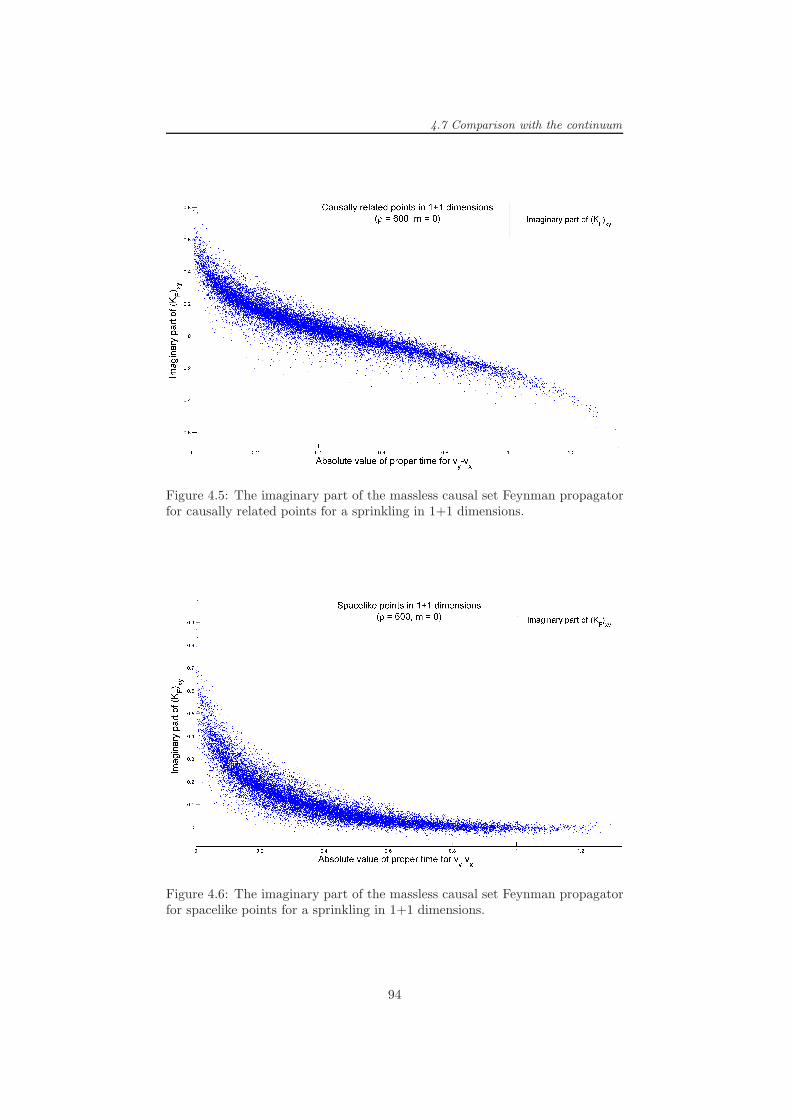
4.7 Comparison with the continuum
Figure 4.5: The imaginary part of the massless causal set Feynman propagatorfor causally related points for a sprinkling in 1+1 dimensions.
Figure 4.6: The imaginary part of the massless causal set Feynman propagatorfor spacelike points for a sprinkling in 1+1 dimensions.
94

4.8 Extensions of the model
4.7.2 3+1 dimensions
Unfortunately, as with the retarded propagator, in 3+1 dimensions the simu-
lations are less clear. We only expect good agreement with the continuum for
large ρ since the infinite density limit is needed in (4.53). The only way to get
a large density simulation without a large causal set is to sprinkle a moderate
number of points into a small spacetime volume. The behaviour is then only in-
vestigated for small proper times and comparisons are difficult because the small
proper-time behaviour of G(4)F is singular, being dominated by delta-functions
and divergent Bessel functions.
Larger sprinklings are needed to investigate further any agreement between
KF and G(4)F for a range of proper times. For what it’s worth we present the
plots for ρ = 480625 m = 10 in Figure 4.7 and Figure 4.8. Encouraged by
the 1+1 dimensional results we expect to see agreement when it is possible to
simulate large densities over a large volume.
4.8 Extensions of the model
The model we’ve defined so far deals only with a real scalar field on a finite
causal set. We now discuss extending the model to complex scalar fields and
infinite causal sets.
4.8.1 Complex scalar fields
The formalism described so far extends without difficulty to complex scalar
fields. The simplest way to achieve this extension is to use two real scalar fields
φa and φb (with the same mass m) which, in addition to conditions 1-3, satisfy
[(φa)x, (φb)y ] = 0, (4.56)
for all x, y = 1, . . . , p.
We then define
Φx :=1√2
((φa)x + i(φb)x
), (4.57)
to be our complex scalar field.
This satisfies
1. [Φ†x, Φy] = i∆xy, [Φx, Φy] = [Φ†
x, Φ†y] = 0 (4.58)
2. i∆w =⇒p∑
x′=1
wx′Φx′ = 0 (4.59)
95

4.8 Extensions of the model
Figure 4.7: The imaginary part of the causal set Feynman propagator for acausally related points for a sprinkling in 3+1 dimensions.
Figure 4.8: The imaginary part of the causal set Feynman propagator for aspacelike points for a sprinkling in 3+1 dimensions.
96

4.8 Extensions of the model
These two conditions could in fact have been used to define the complex
scalar field theory, proceeding along the same lines as in the real case—the
steps are entirely analogous.
4.8.2 Non-finite causal sets
The formalism presented so far is only defined for finite causal sets. For finite
p-element causal sets the matrix i∆ is a finite p × p Hermitian matrix. This
is guaranteed to possess p eigenvalues and p eigenvectors and, using these, the
field operators φx (x = 1, . . . , p) can be written as
φx =
s∑
i=1
√λi(ui)xai +
√λi(vi)xa
†i . (4.40)
for s pairs of creation and annihilation operators a†i and ai.
When the causal set is infinite there are two difficulties which are encoun-
tered when trying to define the field operators in this way.
Eigenvectors of Pauli-Jordan function
Firstly, on the positive side, we note that since a causal set is locally finite i∆
is well-defined for any causal set. On the negative side, when the causal set
is infinite, i∆ takes the form of an infinite matrix and many of the operations
that can be performed on finite matrices do not carry over to infinite ones12.
Instead, the correct way to treat i∆ is as an operator on a Hilbert space, say
(if the causal set is countable) the space of infinite square-summable sequences
of complex numbers, denoted ℓ2.
If ψ = (ψ1, ψ2, . . .) ∈ ℓ2 is an infinite sequence of complex numbers (such
that∑∞
x=1 |ψx|2 <∞) then the action of i∆ on ψ is the infinite sequence
(i∆ψ)x :=∞∑
y=1
i∆xyψy, (4.60)
where x = 1, 2, . . . ,∞. For a general causal set13 however, these infinite sums
may not converge for particular values of x and, even if the sums do converge
for all x, the sequence (i∆ψ)x may not be a vector in ℓ2 (i.e. we may not have∑∞
x=1 |(i∆ψ)x|2 <∞).
Nevertheless, even though, for a particular causal set, i∆ may not define an
operator valid for all ψ ∈ ℓ2 there will exist ψ ∈ ℓ2 such that the sequence (i∆ψ)x
12See Stone (1932, Chapter III, §1) for a full discussion.13The convergence of these sums depends on the particular causal set as well as the choice
of model for the retarded propagator.
97

4.8 Extensions of the model
is a vector in ℓ2. As an example i∆ acting on the zero vector 0 = (0, 0, . . .) is
always in ℓ2, i.e. i∆0 = 0. We therefore expect that the action of i∆ will be only
well-defined on a domain D(i∆) ⊆ ℓ2 (in some special cases D(i∆) may equal
ℓ2, i.e. when∑∞
x=1 |∑∞
y=1 i∆xyψy|2 < ∞ for all ψy ∈ ℓ2). The full machinery
of operators defined on domains will be covered in the next chapter (see Section
5.1 for a full explanation of the terms about to be employed).
If we are lucky enough that i∆ defines a self-adjoint operator then we can
try to repeat the procedure we followed for a finite causal set to define the
field operators. If i∆ possesses an orthonormal basis of eigenvectors (i.e. if
it has a countable point spectrum (Jordan, 1969, p51)) then we can use these
eigenvectors and eigenvalues to define φx operators analogously to (4.40), the
summation presumably now being an infinite one. We could then attempt to
use this expression for the field operators to develop the theory, although we
would expect to encounter issues of convergence relating to the sums involved.
Unfortunately, even if i∆ is self-adjoint, it may not possess any eigenvalues
or eigenvectors (Jordan, 1969, p44). In this case we would be unable to use
eigenvectors of i∆ to define the field operators φx (simply because there would
be no eigenvectors!). Nevertheless we could use spectral theory to define an
analogue of the two-point function Q when i∆ is self-adjoint. If the spectral
family of i∆ is Ex (see Section 5.1.3 for definitions) then we have
(ψ, i∆φ) =
∫ ∞
−∞xd(ψ, Exφ), (4.61)
for ψ, φ ∈ D(i∆). We can define the two-point function Q to be the operator
defined by taking the “positive part” of this:
(ψ,Qφ) :=
∫ ∞
0
xd(ψ, Exφ). (4.62)
It would then be possible to define the Feynman propagator as KF = KR + iQ.
We could then try to proceed by just using these “infinite matrices” without
ever mentioning field operators (for example, trying to sum Feynman diagrams
on the causal set without mentioning operators).
Creation and annihilation operators
Another difficulty in extending the model to infinite causal sets is that, even if
we were able to find appropriate ui and vi eigenvectors and wrote down φx in
the form (4.40) then, presumably, we would have an infinite number of creation
and annihilation operators a†i and ai, i = 1, 2, . . . ,∞ satisfying
[a†i , aj] = δij , [a†i , a†j ] = [ai, aj ] = 0. (4.63)
98

4.9 0+1 dimensional calculation
Since there are infinitely many pairs of these operators the Stone-von-Neumann
theorem does not apply—there will exist unitarily-inequivalent representations
of these commutation relations as operators on a Hilbert space. The question
arises, therefore, which representation should we choose? We make no attempt
to answer this question but point out that its resolution may require us to
introduce another condition on the ai and a†i which would restore the uniqueness
of their representation.
Discussion
It is clear from the two problems just described that there are mathematical
difficulties in generalising the definition of field operators (4.40) from a finite
causal set to an infinite one. It appears that these difficulties, however, depend
heavily on the particular causal set that is being used. For some infinite causal
sets (e.g. the infinite antichain where i∆xy = 0 for all x, y = 1, 2, . . .) the theory
is simple (i.e. φx = 0 for all x) whereas for others one can imagine that the
domain of i∆ and a determination of its eigenvectors (if they exist at all) is
much more complicated. It’s possible that the current model only extends to
a certain class of infinite causal sets and that substantial modification will be
needed if it is to extend to all infinite causal sets.
An obvious way out of these difficulties is to only use finite (extremely large)
causal sets as a model for spacetime. The field operators are well-defined for
any finite causal set and for all practical purposes a very large but finite causal
set would serve perfectly well as a model for spacetime (consider, for example,
a Planckian density sprinkling into a Lorentzian manifold modelling the entire
observable universe!).
4.9 0+1 dimensional calculation
It is hard to calculate the eigen-decomposition of i∆ for general causal sets
analytically. For a totally ordered causal set, however, it is possible.
Recall from Section 3.10.1 that the retarded propagator for a p-element
sprinkling into 0+1 dimensions is given by (3.83) (here we again use the natural
labelling v1 ≺ v2 ≺ . . . ≺ vp):
(KR)xy =
2 sin(2(y − x) arcsin
(m2ρ
))
m√4− m2
ρ2
if x < y
0 if x ≥ y.
(4.64)
99

4.9 0+1 dimensional calculation
for x, y = 1, . . . , p.
Using this we see that i∆ = i(KR −KA) takes the form
i∆xy =2i sin
(2(y − x) arcsin
(m2ρ
))
m√4− m2
ρ2
, (4.65)
for x, y = 1, . . . , p.
There are p − 2 eigenvectors which have 0 as an eigenvalue. These are p-
component column vectors of the (unnormalised) form
wk := ρ2(~ek−1 − 2~ek + ~ek+1) +m2~ek, (4.66)
for k = 2, . . . , p− 1 (here ~ei are the standard basis vectors non-zero only in the
ith component). For example
w2 =
ρ2
−2ρ2 +m2
ρ2
0
0...
0
, w3 =
0
ρ2
−2ρ2 +m2
ρ2
0...
0
. (4.67)
We can see that these are eigenvectors because the x-component of the vector
i∆wk is equal to
(i∆wk)x = ρ2i∆x(k−1) −(2ρ2 −m2
)i∆xk + ρ2i∆x(k+1) (4.68)
=2iρ2
m√4− m2
ρ2
(sin ((k−x−1)θ)−
(2−m2
ρ2
)sin ((k−x)θ)+sin ((k−x+1)θ)
),
(4.69)
where θ := 2 arcsin(
m2ρ
). Trigonometric identities can be used to simplify this
and we are left with
(i∆wk)x = 0, (4.70)
for k = 2, . . . , p− 1 and x = 1, . . . , p.
This means that we have found p− 2 eigenvectors which have 0 eigenvalue,
namely the vectors wk defined in (4.66) for k = 2, . . . , p−1. Imposing condition
3 immediately gives constraints on the field operators of the form: ρ2(φx−1 −2φx + φx+1) + m2φx = 0 for x = 2, . . . , p − 1. This is a discretisation of
the 0+1 dimensional Klein-Gordon equation ( + m2)φ(x) = 0. Thus, in the
100

4.10 Rank of the Pauli-Jordan matrix
0+1 case, condition 3 serves to enforce an appropriate version of the Klein-
Gordon equation. The 2 remaining non-zero eigenvalues are harder to obtain
analytically.
4.10 Rank of the Pauli-Jordan matrix
In the 0+1 dimensional example just studied we saw that the vast majority of
the eigenvalues were 0. This is peculiar to sprinklings into M1. For sprinklings
into higher dimensions the number of 0 eigenvalues is much less.
The number of 0 eigenvalues for a p-element sprinkling is p− 2s where 2s is
the rank of i∆ (2s is also the rank of ∆, the factor of i makes no difference).
Here we investigate how this quantity changes as we increase the sprinkling
density. We will look at sprinklings into a fixed causal interval in M2 at different
densities.
4.10.1 Mass dependence
Firstly we note that the rank of the Pauli-Jordanmatrix is mass-independent. In
Section 3.10 we found the general form of the retarded propagatorKR (obtained
by summing over trajectories that only go forward in time) to be (3.74):
KR = Φ(I −ΨΦ)−1 = Φ+ΦΨΦ+ ΦΨΦΨΦ+ . . . , (4.71)
where Φ is the matrix of “hop” amplitudes and Ψ is a diagonal matrix of “stop”
amplitudes. Inverting (4.71) gives:
Φ = KR(I +ΨKR)−1 = KR −KRΨKR +KRΨKRΨKR − . . . . (4.72)
In keeping with the mass scattering ideas of Section 3.9 we assume that when
the mass is zero we have KR = Φ. In this case the massive Pauli-Jordan matrix
is ∆m := KR − KTR and the massless Pauli-Jordan matrix is ∆0 := Φ − ΦT .
We can show that these two matrices have the same null space14, i.e. ∆mw =
0 ⇐⇒ ∆0w = 0. To see this we use (4.71) and (4.72) to give:
∆0w = 0 ⇐⇒ Φw = ΦTw ⇐⇒ KRw = KTRw ⇐⇒ ∆mw = 0, (4.73)
where we have used that Ψ = ΨT .
Since the null spaces of the matrices are the same this shows that the rank of
the massive Pauli-Jordan matrix equals the rank of the massless Pauli-Jordan
14The null space of a matrix is the vector space spanned its 0-eigenvalue eigenvectors.
101

4.11 Calculation in the continuum
matrix. Therefore in our investigation it is sufficient to look at p − 2s for the
massless Pauli-Jordan function.
4.10.2 Density dependence
We can investigate the dependence of p − 2s on the sprinkling density by per-
forming the following steps:
1. Let ρ take values from ρmin to ρmax in increments of ρinc.
2. For each ρ sprinkle a causal set into a causal interval in Md of unit volume.
3. Calculate p − 2s (i.e. the number of 0 eigenvalues of i∆) for the causal
set.
4. Repeat steps 2 and 3 for N sprinklings and take the average of these N
numbers.
5. Plot this average for each density ρ.
The result of this is shown in Figure 4.9 for ρmin = 100, ρmax = 500, ρinc =
20, d = 2, N = 1000. As we can see there is a steady increase in the number of
0 eigenvalues as the density increases.
The number of creation and annihilation operators needed to define the field
operators φx is 2s. The results of Figure 4.9 show that 2s increases only slightly
slower than the number of causal set elements p (for the sprinklings used in the
Figure the expected value of p is ρ). This is in contrast to the continuum where
the number of creation and annihilation operators is infinite (usually indexed
by spatial-momentum), regardless of the size of the region.
4.11 Calculation in the continuum
The idea of using the eigenvectors and eigenvalues of the Pauli-Jordan function
as a way to derive the Feynman propagator seems to be a new one. We can try
to perform the same procedure in the continuum.
4.11.1 Preliminaries
Suppose we know the Pauli-Jordan function i∆(x, y) for a spacetime region R.
We shall just work in flat spacetimes for which this is a translation-invariant
function depending only on x− y. For curved spacetimes this would depend on
x and y individually.
102
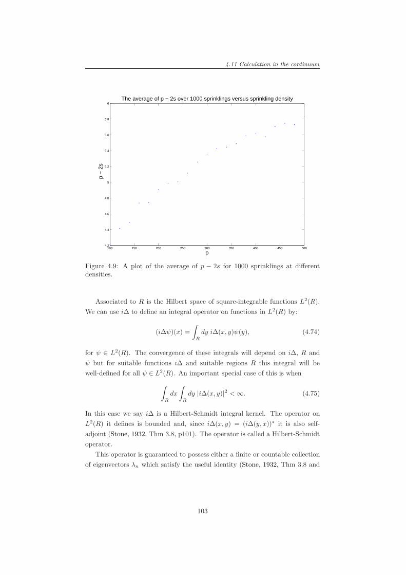
4.11 Calculation in the continuum
100 150 200 250 300 350 400 450 5004.2
4.4
4.6
4.8
5
5.2
5.4
5.6
5.8
6The average of p − 2s over 1000 sprinklings versus sprinkling density
ρ
p −
2s
Figure 4.9: A plot of the average of p − 2s for 1000 sprinklings at differentdensities.
Associated to R is the Hilbert space of square-integrable functions L2(R).
We can use i∆ to define an integral operator on functions in L2(R) by:
(i∆ψ)(x) =
∫
R
dy i∆(x, y)ψ(y), (4.74)
for ψ ∈ L2(R). The convergence of these integrals will depend on i∆, R and
ψ but for suitable functions i∆ and suitable regions R this integral will be
well-defined for all ψ ∈ L2(R). An important special case of this is when
∫
R
dx
∫
R
dy |i∆(x, y)|2 <∞. (4.75)
In this case we say i∆ is a Hilbert-Schmidt integral kernel. The operator on
L2(R) it defines is bounded and, since i∆(x, y) = (i∆(y, x))∗ it is also self-
adjoint (Stone, 1932, Thm 3.8, p101). The operator is called a Hilbert-Schmidt
operator.
This operator is guaranteed to possess either a finite or countable collection
of eigenvectors λn which satisfy the useful identity (Stone, 1932, Thm 3.8 and
103

4.11 Calculation in the continuum
Thm 5.14): ∫
R
dx
∫
R
dy |i∆(x, y)|2 =∑
n
λ2n, (4.76)
If f ∈ L2(R) is an eigenvector of i∆ then it satisfies
∫
R
dy i∆(x, y)f(y) = λf(x). (4.77)
Applying x +m2 to both sides and using that (x +m2)i∆(x, y) = 0 we have
that if f(x) is an eigenvector with non-zero eigenvalue then it is a solution of the
Klein-Gordon equation: (+m2)f(x) = 0. This is a helpful aid when trying to
determine the eigenvectors. The eigenvectors are defined up to a normalisation
and a phase factor.
If we succeed in determining all the eigenvectors with non-zero eigenvalues
then we can define the two-point function to be
Q(x, y) =∑
λ>0
λf(x)f(y)∗, (4.78)
where we sum over all eigenvalue-eigenvector pairs (λ, f) with λ > 0 and the f
are normalised: ||f || = 1 where ||f ||2 =∫Rdx |f(x)|2. We shall concentrate on
the two-point function because if we know that then we can define the Feynman
propagator (as the sum of the retarded propagator and iQ(x, y), see (4.49)).
4.11.2 Causal interval in 0+1 dimensional Minkowski space-
time
As a warm-up exercise we examine the eigen-decomposition of i∆ for a causal
interval in M1. We suppose our interval extends from x = −L to x = L so our
region is R = [−L,L]. In M1 the d’Alembertian and the massive Pauli-Jordan
function are (see (3.12)):
=∂2
∂x2, ∆(x) =
sin(mx)
m. (4.79)
We have
∫ L
−L
dx
∫ L
−L
dy|i∆(x− y)|2 =8L2m2 + cos(4Lm)− 1
4m4, (4.80)
which shows that i∆ defines a Hilbert-Schmidt integral operator on L2([−L,L]).The eigenvectors of i∆ with non-zero eigenvalue satisfy ( +m2)f(x) = 0.
104

4.11 Calculation in the continuum
They must therefore take the form
f(x) = A cos(mx) +B sin(mx), (4.81)
for some constants A and B.
We have
f i∆f
sin(mx)
(i sin(2Lm)
2m2− iL
m
)cos(mx)
cos(mx)
(i sin(2Lm)
2m2+iL
m
)sin(mx)
Comparing the coefficients of sin(mx) and cos(mx) and normalising the
eigenvectors we find that
f+(x) :=
√m cos(mx)√
2Lm+ sin(2Lm)+
i√m sin(mx)√
2Lm− sin(2Lm), (4.82)
f−(x) :=
√m cos(mx)√
2Lm+ sin(2Lm)− i
√m sin(mx)√
2Lm− sin(2Lm), (4.83)
satisfy
i∆f+ = λf+, i∆f− = −λf−, (4.84)
where
λ =
√2Lm− sin(2Lm)
√2Lm+ sin(2Lm)
2m2. (4.85)
We see that ±λ are the only non-zero eigenvalues because
λ2 + (−λ)2 =8L2m2 + cos(4Lm)− 1
4m4=
∫ L
−L
dx
∫ L
−L
dy|i∆(x− y)|2, (4.86)
(compare with (4.76)).
The two-point function
Usually we would define the two-point function to be the sum over all the
positive eigenvectors. This time, however, we only have one non-zero eigenvalue.
This gives:
Q(x, y) := λf+(x)f+(y)∗. (4.87)
105

4.11 Calculation in the continuum
The real and imaginary parts of this function are
ℜ[Q(x, y)] =1
2mCcos(mx) cos(my) +
C
2msin(mx) sin(my) (4.88)
ℑ[Q(x, y)] =sin(mx) cos(my)
2m− cos(mx) sin(my)
2m=
∆(x− y)
2(4.89)
where
C =
√2Lm+ sin(2Lm)√2Lm− sin(2Lm)
. (4.90)
Noticing that limL→∞ C = 1 therefore gives
limL→∞
Q(x, y) =exp(im(x− y))
2m, (4.91)
which is precisely the continuum two-point function.
For finite L the real part ℜ[Q(x, y)] differs from the real part of the con-
tinuum two-point function due to the calculation being done in a finite sized
interval.
4.11.3 Causal interval in 1+1 dimensional Minkowski space-
time
A more interesting example is that of a massless scalar field in a finite causal
interval in M2. We shall work in light-cone coordinates
u =t+ x√
2v =
t− x√2. (4.92)
For a fixed finite length L the range of these coordinates will be restricted to
u, v ∈ [−L,L]. Our attention is therefore restricted to the region R = [−L,L]×[−L,L].
In these coordinates the 2-dimensional d’Alembertian is simply
= 2∂2
∂u∂v, (4.93)
and the Pauli-Jordan function is (see (3.13))
∆(u, v) =1
2(θ(u)θ(v) − θ(−u)θ(−v)) = 1
2(θ(u) + θ(v)− 1). (4.94)
We have
∫ L
−L
du
∫ L
−L
du′∫ L
−L
dv
∫ L
−L
dv′|i∆(u− u′, v − v′)|2 = 2L4, (4.95)
106

4.11 Calculation in the continuum
which shows that i∆ defines a Hilbert-Schmidt operator.
Eigenvectors and Eigenvalues
The eigenvectors of i∆ with non-zero eigenvalue satisfy f = 0. The most
general form of such solutions is f(u, v) = f1(u) + f2(v) for arbitrary functions
f1, f2 ∈ L2([−L,L]).By considering how i∆ acts on particular functions we will be able to iden-
tify the eigenvectors. The action of i∆ is evaluated by simply performing the
integration.
f i∆f
eikuL
keiku − L
kcos(kL) + i
v
ksin(kL)
eikvL
keikv − L
kcos(kL) + i
u
ksin(kL)
1 iL(u+ v)
Using these results we can obtain two families of eigenvectors fk and gk given
by15:
fk(u, v) := eiku − eikv, with k =nπ
L, n = ±1,±2, . . . (4.96)
gk(u, v) := eiku + eikv − 2 cos(kL), with tan(kL) = 2kL, k 6= 0 (4.97)
These satisfy
(i∆fk)(u, v) =L
kfk(u, v), (i∆gk)(u, v) =
L
kgk(u, v). (4.98)
As written these eigenvectors are unnormalised. By direct computation the
square of their L2(R) norms are ||fk||2 = 8L2 and ||gk||2 = 8L2−16L2 cos2(kL).
For the gk family of eigenvectors the k parameter satisfies the transcendental
equation tan(kL) = 2kL. This has a countably infinite number of real solutions
(see Figure 4.10).
We now show that the fk and gk families are the only eigenvectors with non-
zero eigenvalues. We do this, as in the 0+1 case, by summing the eigenvalues
15The gk family were found by Rafael Sorkin.
107
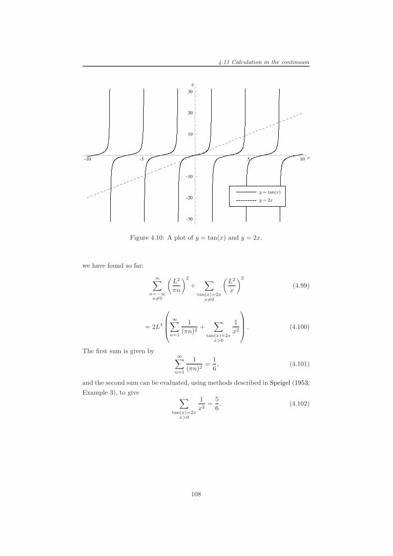
4.11 Calculation in the continuum
Figure 4.10: A plot of y = tan(x) and y = 2x.
we have found so far:
∞∑
n=−∞n6=0
(L2
πn
)2
+∑
tan(x)=2xx 6=0
(L2
x
)2
(4.99)
= 2L4
∞∑
n=1
1
(πn)2+
∑
tan(x)=2xx>0
1
x2
. (4.100)
The first sum is given by∞∑
n=1
1
(πn)2=
1
6, (4.101)
and the second sum can be evaluated, using methods described in Speigel (1953,
Example 3), to give∑
tan(x)=2xx>0
1
x2=
5
6. (4.102)
108

4.11 Calculation in the continuum
We therefore have that
2L4 =
∞∑
n=−∞n6=0
(L2
πn
)2
+∑
tan(x)=2xx 6=0
(L2
x
)2
(4.103)
=
∫ L
−L
du
∫ L
−L
du′∫ L
−L
dv
∫ L
−L
dv′|i∆(u− u′, v − v′)|2, (4.104)
which shows that we have found all the non-zero eigenvalues (compare with
(4.76)).
The two-point function
Having found all the non-zero eigenvalues and corresponding eigenvectors we
are interested in obtaining the analogue of the two-point function by summing
over the positive eigenvalues.
We define
Q(u, v, u′, v′) :=
∞∑
n=1
L2
πn
1
||fk||2fk(u, v)fk(u
′, v′)∗
+∑
tan(x)=2xx>0
L2
x
1
||gk||2gk(u, v)gk(u
′, v′)∗, (4.105)
where ||fk||2 = 8L2 and ||gk||2 = 8L2 − 16L2 cos2(kL) are included to ensure
we’re summing over products of normalised eigenvectors.
It seems formidable to evaluate this sum in closed-form. We can, however,
approximate it by computing the sum over a finite number of eigenvalues nu-
merically. As with the 0+1 case of the previous section the function is not
translation invariant (i.e. it depends on u, v, u′, v′ separately, not just on their
differences u− u′, v − v′).
We plot the real and imaginary parts of Q(u, v, 0, 0) for L = 1 in Figure
4.11 and Figure 4.12. To make the plots we summed over roots of tan(x) = 2x
between 0 and 1000. It is clear from Figure 4.12 that the imaginary part of
Q(u, v, 0, 0) is approaching ∆(u, v)/2. The real part of Q(u, v, 0, 0) certainly
seems to approach a well-defined function but the analytic form of it is not yet
known.
The massive case
The massive Pauli-Jordan function in M2 is given by a Bessel function which
decays inside the future and past lightcones. This is bounded above by the mass-
less Pauli-Jordan function and, as such, defines a Hilbert-Schmidt operator. We
109

4.11 Calculation in the continuum
−1−0.8
−0.6−0.4
−0.20
0.20.4
0.60.8
1
−1
−0.8
−0.6
−0.4
−0.2
0
0.2
0.4
0.6
0.8
1
−0.2
0
0.2
0.4
0.6
0.8
1
1.2
u
Plot of ℜ [Q(u,v,0,0)]
v
Figure 4.11: The real part of an approximation to Q(u, v, 0, 0) for L = 1.
−1−0.8
−0.6−0.4
−0.20
0.20.4
0.60.8
1
−1
−0.8
−0.6
−0.4
−0.2
0
0.2
0.4
0.6
0.8
1
−0.4
−0.3
−0.2
−0.1
0
0.1
0.2
0.3
0.4
u
Plot of ℑ [Q(u,v,0,0)]
v
Figure 4.12: The imaginary part of an approximation to Q(u, v, 0, 0) for L = 1.
110
4.11 Calculation in the continuum
would like to be able to compute the eigendecomposition for the massive case
but have been unable to do due to the complicated integrals involved. Neverthe-
less since it is a Hilbert-Schmidt operator it does have an eigendecomposition
and, in principle, the two-point function could be computed.
It remains possible that the eigendecomposition or the two-point function
could be computed by another, less direct, method (e.g. using the Fourier
transform). It may be possible, for example, to compute the two-point func-
tion directly, without recourse to the eigen-decomposition of i∆ (e.g. taking
inspiration from (4.31)).
4.11.4 Unbounded regions
The two examples just considered restrict attention to bounded regions R ⊂ Md.
If we try to apply the same ideas to unbounded regions, say the whole of Md,
we encounter divergent expressions. If we ignore these divergences and treat
the objects formally we can, with a little care, still obtain the correct two-point
function.
0+1 dimensional Minkowski spacetime
As a warm-up we consider the calculation in M1. As before
i∆(x) =i sin(mx)
m=
1
2m
(eimx − e−imx
). (4.106)
This defines an integral operator on functions on M1 by
(i∆f)(x) =
∫dyi∆(x− y)f(y), (4.107)
where we now integrate over all of M1 = R (not just an interval from −L to L).
For fc(x) := eicx this gives
(i∆fc)(x) =1
2m
(δ(c−m)eimx − δ(c+m)e−imx
)(4.108)
From this we find that as c varies we obtain a family of eigenvectors:
• If c 6= ±m then i∆fc = λcfc = 0.
• If c = m then i∆fm = λmfm.
• If c = −m then i∆f−m = −λ−mf−m.
where we have defined
λc := ǫ(c)δ(c−m) + δ(c+m)
2m= ǫ(c)δ(c2 −m2). (4.109)
111

4.11 Calculation in the continuum
where
ǫ(α) :=
1 if α > 0,
0 if α = 0,
−1 if α < 0.
(4.110)
Note that λm and λ−m are divergent, being proportional to δ(0).
These eigenvectors are orthogonal and normalised as
∫dxf∗
c (x)fc′(x) = δ(c− c′) (4.111)
From (4.109) we see the sign of any non-zero eigenvalue λc is equal to ǫ(c)
(treating δ(0) as a positive number!).
We define the two-point function by integrating over all eigenvectors but
setting the contribution from the negative eigenvalues to zero (this is achieved
by a factor of θ(ǫ(c)) in the integral). This gives:
Q(x, y) :=
∫ ∞
−∞dc θ(ǫ(c))λcfc(x)fc(y)
∗ (4.112)
=
∫ ∞
0
dcδ(c−m)
2meicxe−icy =
1
2meim(x−y) (4.113)
which is precisely the continuum two-point function!
3+1 dimensional Minkowski spacetime
The same arguments apply to the calculation in Md for general d. Here we look
at the d = 4 case where we have (Bogoliubov and Shirkov, 1959, Appx I, §B):
i∆(x) =1
(2π)3
∫d4pǫ(p0)δ(p
2 −m2)eipx =1
(2π)3
∫d3~p
1
2ω~p
(eipx − e−ipx
)
(4.114)
where p := (p0, ~p) is a general momentum 4-vector and p := (ω~p, ~p) is an on-shell
momentum 4-vector with ω~p :=√~p2 +m2.
Treating this as an integral operator acting on functions on M4 we have:
(i∆f)(x) :=
∫d4yi∆(x− y)f(y) (4.115)
where we integrate over all of M4.
For fk(x) := eikx where k = (k0, ~k) is a general momentum 4-vector (not
112

4.11 Calculation in the continuum
necessarily on shell) we have that
(i∆fk)(x) =1
(2π)3
∫d4y
∫d3~p
1
2ω~p
(eip(x−y) − e−ip(x−y)
)eiky (4.116)
=1
(2π)3
∫d3~p
1
2ω~p
(eipxδ4(k − p)− e−ipxδ4(k + p)
)(4.117)
=1
(2π)31
2ω~k
(eikxδ(k0 − ω~k)− e−ikxδ(k0 + ω~k)
)(4.118)
where k := (ω~k,~k) is on-shell.
We thus have the following family of eigenvectors:
• If k0 6= ±ω~k then i∆fk = λkfk = 0.
• If k0 = ω~k then i∆fk = λkfk.
• If k0 = −ω~k then i∆f−k = −λkf−k.
where
λk :=1
(2π)3ǫ(k0)
δ(k0 − ω~k) + δ(k0 + ω~k)
2ω~k=
1
(2π)3ǫ(k0)δ(k
2 −m2) (4.119)
Note that, unlike the 0+1 calculation, here the non-zero eigenvalues appear
with multiplicity—there are multiple eigenvectors for each eigenvalue.
The eigenvectors are orthogonal and normalised as
∫d4xfk(x)
∗fk′(x) = δ4(k − k′). (4.120)
We see the sign of any non-zero eigenvalue λk is equal to ǫ(k0). To de-
fine the two-point function we therefore sum over all eigenvectors but set the
contribution from the negative eigenvalues to zero:
Q(x, y) :=
∫d4k θ(ǫ(k0))λkfk(x)fk(y)
∗ (4.121)
=1
(2π)3
∫d4k θ(k0)δ(k
2 −m2)eik(x−y) (4.122)
which is exactly the continuum two-point function (Bogoliubov and Shirkov,
1959, Appx I, §B)!
Discussion
The calculations in an unbounded region require working with divergent formal
expressions (e.g. eigenvalues proportional to δ(0)). Nevertheless formal manip-
ulations of such expressions do lead to the correct two-point function. It may
113

4.12 Mode expansions
be possible, therefore, to redo the calculations in a rigorous manner. This could
involve (i) using the theory of distributions or (ii) working in a bounded region
and taking the limit as the region tends to the unbounded region (compare
(4.91)).
It is also interesting to investigate what we get when this method for ob-
taining the two-point function is applied to other spacetimes. This has been
investigated by Hustler (2010) for Rindler spacetime.
4.12 Mode expansions
In continuum scalar quantum field theory in M4 the field φ(x) can be expanded
in terms of creation and annihilation operators in the form
φ(x) =
∫d3~p
1
2ω~p
(a~pe
ipx + a†~pe−ipx
), (4.123)
where ω~p :=√~p2 +m2 and a†~p and a~p are the creation and annihilation opera-
tors for a particle of on-shell 4-momentum (ω~p, ~p). Similar decompositions hold
in other dimensions.
When we compare this to the expansion for our field operators:
φx =
s∑
i=1
√λi(ui)xai +
√λi(vi)xa
†i , (4.40)
it is tempting to identify the combination√λi(ui)x as playing the role of the
plane-waves 12ω~p
eipx. We would then be able to identify particular eigenvectors
ui as corresponding to particular on-shell momenta.
To better understand the behaviour of the eigenvectors we look back at
the continuum calculation in 1+1 dimensions from Section 4.11.3. There the
eigenvectors were of the form
fk(u, v) := eiku − eikv, with k =nπ
L, n = ±1,±2, . . . (4.96)
gk(u, v) := eiku + eikv − 2 cos(kL), with tan(kL) = 2kL, k 6= 0 (4.97)
We see that each fk and gk is a linear combination of plane-waves with on-shell
null 2-momenta of energy k (with an additional constant term appearing in gk).
In particular there is no multiplicity here—each eigenvalue appears once only.
On the other hand, if we look at the continuum calculation in M4 from
Section 4.11.4 we see the eigenvectors are plane-waves (albeit with divergent
eigenvalues). In addition the eigenvalues λk appear with multiplicity—there are
multiple plane-waves with the same eigenvalue.
114

4.12 Mode expansions
In light of this we suggest the following behaviour. It seems that for sprin-
klings into finite regions of Md the eigenvectors of the causal set Pauli-Jordan
function do not correspond to plane-waves but rather to superpositions of plane-
waves (at a fixed energy). As the sprinkling region gets larger and larger the
eigenvalues get bunched closer together, e.g. for large causal sets we might
have an eigenvalue as λ = 50 and another at λ′ = 50.1 etc. The corresponding
eigenvectors almost share the same eigenvalue. Linear combinations of these
eigenvectors may then approximate a plane-wave with an energy related to the
eigenvalue. In the limit when the region is the whole of Md the eigenvalues
appear with multiplicity and the eigenvectors correspond to plane-waves.
This speculative description would bridge the gap between the continuum
calculations in bounded and unbounded regions. If it’s really what’s going
on then for large causal sets sprinkled into Md we should be able to obtain
eigenvectors (or linear combinations of eigenvectors) to serve as plane-waves.
We can study the behaviour of the eigenvectors for particular sprinklings
into finite regions of Md on a computer. We regard the x-component of an
eigenvector as assigning a complex number to the xth causal set element. In
two-dimensions we can display this as a 3-dimensional plot where two axes are
the element’s position in M2 and the third axis is the real or imaginary part of
the eigenvector component.
In Figure 4.13 and Figure 4.14 we plot the real and imaginary parts of
the eigenvector (which we denote u1) associated with the largest eigenvalue of
i∆, for a sprinkling into a causal interval in M2. In the plot the dots denote
the values of (u1)x at the xth sprinkled point. The surface is an interpolation
between them (we hope there is no confusion between the coordinate u and
the eigenvector u1). Interestingly the eigenvectors associated with the largest
eigenvalues show relatively smooth oscillating behaviour. There are oscillations
in more than one direction which suggests that the eigenvectors best correspond
to a sum of plane-waves—if they corresponded to a single plane-wave then the
peaks and troughs would proceed in a single spacetime direction.
The eigenvectors associated with the smaller eigenvalues show less smooth,
more jagged behaviour (as shown in Figure 4.15 and Figure 4.16).
In light of Section 4.11.4 it appears the eigenvalue can be related to the en-
ergy of the plane-wave. Since the mass-dimensions of the causal set eigenvalues
are [λi] =Md−2 the quantity
Ei :=
√ρ
λi, (4.124)
has dimensions of energy: [Ei] =M . This suggests that Ei could be interpreted
(up to a dimensionless proportionality constant) as the energy associated with
115

4.12 Mode expansions
−1 −0.8 −0.6 −0.4 −0.2 0 0.2 0.4 0.6 0.8 1−1
−0.5
0
0.5
1
−0.05
−0.04
−0.03
−0.02
−0.01
0
0.01
0.02
0.03
0.04
0.05
v
u
Plot of ℜ [u1] as a function of position (ρ = 1000, m = 8, λ = 66)
Figure 4.13: The real part of u1 for ρ = 1000,m = 8 with eigenvalue λ1 = 66.
−1 −0.8 −0.6 −0.4 −0.2 0 0.2 0.4 0.6 0.8 1−1
−0.5
0
0.5
1
−0.05
−0.04
−0.03
−0.02
−0.01
0
0.01
0.02
0.03
0.04
0.05
v
u
Plot of ℑ [u1] as a function of position (ρ = 1000, m = 8, λ = 66)
Figure 4.14: The imaginary part of u1 for ρ = 1000,m = 8 with eigenvalueλ1 = 66.
116

4.12 Mode expansions
−1−0.8
−0.6−0.4
−0.20
0.20.4
0.60.8
1
−1
−0.8
−0.6
−0.4
−0.2
0
0.2
0.4
0.6
0.8
1
−0.08
−0.06
−0.04
−0.02
0
0.02
0.04
0.06
0.08
u
Plot of ℜ [u] as a function of position (ρ = 1000, m = 8, λ = 0.16)
v
Figure 4.15: The real part of an eigenvector u for ρ = 1000,m = 8 with eigen-value λ = 0.16.
−1−0.8
−0.6−0.4
−0.20
0.20.4
0.60.8
1
−1
−0.8
−0.6
−0.4
−0.2
0
0.2
0.4
0.6
0.8
1
−0.08
−0.06
−0.04
−0.02
0
0.02
0.04
0.06
0.08
u
Plot of ℑ [u] as a function of position (ρ = 1000, m = 8, λ = 0.16)
v
Figure 4.16: The imaginary part of an eigenvector u for ρ = 1000,m = 8 witheigenvalue λ = 0.16.
117

4.12 Mode expansions
the eigenvector ui. This would agree with the smooth behaviour of “low energy”
(large eigenvalue) eigenvectors and the jagged behaviour of “high energy” (small
eigenvalue) eigenvectors.
In addition the sign of the energy could also be identified with the sign of the
eigenvalue: i.e. the ui would have positive energy and the vi would have negative
energy. This would agree with the the continuum two-point function which is a
sum over plane-wave modes of positive energy (Bogoliubov and Shirkov, 1959,
Appx I, §B) (whereas the causal set Q matrix is a sum over the eigenspace
spanned by the ui eigenvectors).
We should mention that since energy is a frame-dependent quantity we have
to decide what frame these statements refer to. For sprinklings into a finite
causal interval the causal interval picks out a preferred time-axis (i.e. the axis
through the end-points of the interval). Presumably the energy assigned to the
eigenvectors is the energy of the plane-waves in a frame with this time-axis.
4.12.1 Preferred set of modes
An important aspect in conventional quantum field theory in curved space-
times is the lack of a preferred choice of modes with which to expand the field
(Birrell and Davies, 1982, p45). Taking inspiration from the causal set model it
is possible that the eigenvectors of the Pauli-Jordan function could be used to
expand the field in an arbitrary curved spacetime (or possibly a finite sub-region
of such a spacetime).
As mentioned in Section 3.13.2 the Klein-Gordon equation in a globally
hyperbolic spacetime is guaranteed to possess unique retarded and advanced
Green’s functions. This ensures that the Pauli-Jordan function exists and is
unique. If its eigenvectors could be determined (along the lines of Section 4.11)
then these could be used to either (i) define a field operator expansion or (ii)
define a Feynman propagator directly without mentioning operators. This ap-
proach could provide a unique way to define the Feynman propagator in curved
spacetimes—something which, if possible, would have important ramifications
for the usual theory.
We can phrase this suggestion in another way. The usual theory involves gen-
eralising the field’s Fourier mode-decomposition fromMd to a curved Lorentzian
manifold. In most cases there is no unique way to perform this generalisation.
The present formalism, however, suggests that the Fourier modes and the eigen-
vectors of i∆ coincide in Md. From this point of view it is the eigenvectors of
i∆, not the Fourier modes, which should be generalised to curved spacetimes.
These eigenvectors (if they exist!) would then provide a preferred set of modes
with which to expand the field.
118

Chapter 5
Interacting Quantum Field
Theory
All my efforts up to that point had been directed toward building
a complete convergent theory. Finding out that after all the series
diverged convinced me that was as far as one could go. . . . That was
of course a terrible blow to all my hopes. It really meant that this
whole program made no sense.
Freeman Dyson in Schweber (1994, p565)
In the previous chapter we described a model for free quantum scalar field
theory on a causal set. Here we extend that model to include interactions
between the scalar fields. This takes us one step closer to a realistic theory
since all known matter fields are involved in interactions. Unfortunately there
are, as yet, no known scalar fields in nature. In the next chapter we discuss
possible models for particles with non-zero spin.
Ultimately our aim is to calculate scattering amplitudes and interaction
cross-sections for particular interacting theories. If a physically realistic the-
ory could be modelled on a causal set (this would require modelling spin-half
and spin-one particles) then these scattering amplitudes would differ from their
continuum counterparts because of the causal set discreteness. Comparing the
causal set calculations to experiments would, at the very least, place bounds on
the allowed discreteness scale. A phenomenological approach to this is described
in Section 5.9.
119

5.1 Operators on Hilbert space
5.1 Operators on Hilbert space
We start by reviewing the mathematical tools we shall need in this chapter.
These will be needed to put the free field theory of the previous chapter on a
rigorous foundation from which we can then define the interacting theory.
We assume the reader is already familiar with the basics of Hilbert space
theory (if not, Geroch (1985, Chapter 48-54) and (Simon and Reed, 1972, Chap-
ter II) provide good introductions). Our definitions follow Geroch (1985, Chap-
ter 55-56) and Simon and Reed (1972, Chapter VIII).
5.1.1 Definitions
Let H be a Hilbert space. An operator on H consists of a vector subspace of
D(A) (called the domain of A) ofH together with a linear mapping A : D(A) →H (the domain may be equal to H or it may be strictly contained within it).
An operator whose domain is a proper subset of H is called unbounded. Two
operators D(A), A and D(B), B are equal if D(A) = D(B) and A = B on this
common domain.
An operator D(A), A is an extension an operator D(B), B if D(B) ⊆ D(A)
and A = B whenever both are defined (i.e. on D(B)).
The domain D(A) of an operator is dense in H if, for every v ∈ H and every
ǫ > 0 there exists a vector v′ ∈ D(A) such that ||h−h′|| < ǫ (where || · || denotesthe norm in H). An operator with a dense domain is called densely defined.
The sum of operators D(A), A and D(B), B is the operator with domain
D(A+ B) := D(A) ∩D(B) defined as A+ B on this domain.
The product of operators D(A), A and D(B), B is the operator with domain
D(AB) :=v ∈ D(B) : Bv ∈ D(A)
and defined as AB on this domain.
An operator D(A), A is closed if whenever a sequence of vectors vn ∈ D(A)
converges to a limit vector v and the sequence of vectors Avn converges to a
limit vector u, then v ∈ D(A) and Av = u.
An operator D(A), A is symmetric if (Au, v) = (u, Av) for all u, v ∈ D(A)
(here (·, ·) denotes the inner-product in H).
5.1.2 Adjoint of an operator
LetD(A), A be a densely defined operator onH. We can define another operator
D(A†), A† called the adjoint of A as follows (Simon and Reed, 1972, p252),
(Geroch, 1985, Chapter 56).
We let D(A†) be the set of all v ∈ H such that there exists a u ∈ H with
(Aw, v
)= (w, u), for all w ∈ D(A). (5.1)
120
5.1 Operators on Hilbert space
For each such v ∈ D(A†) we define A†v := u. If D(A) is dense in H then this u
is unique.
An operator D(A), A is self-adjoint if it is equal to its adjoint: D(A) =
D(A†) and A = A† on this common domain.
An operator D(U), U is unitary if D(U) = H and U U † = U †U = I, the
identity operator on H.
Example
Let H = L2(R) be the Hilbert space of square-integrable functions ψ : R → C.
The position operator D(q), q is the operator defined by
D(q) :=
ψ ∈ L2(R) :
∫ ∞
−∞dq |qψ(q)|2 <∞
, (5.2)
and qψ = qψ for ψ ∈ D(q). It can be shown that this operator is self-adjoint
(Geroch, 1985, p331-332).
5.1.3 Spectral theorem
An important result concerning self-adjoint operators is the spectral theory.
This has a number of equivalent definitions and we follow Jordan (1969, §14).We start with a few definitions.
A projection operator D(E), E is a self-adjoint operator defined on all of H(i.e. D(E) = H) such that E2 = E.
A family of projection operators Ex depending on a real parameter x is a
spectral family if it satisfies:
1. If x ≤ y then Ex ≤ Ey (meaning ExEy = EyEx = Ex),
2. For ǫ > 0 we have Ex+ǫv → Exv as ǫ→ 0 for any v ∈ H and any x ∈ R,
3. Exv → 0 as x→ −∞ and Exv → v as x→ +∞ for any vector v ∈ H.
For any self-adjoint operator D(A), A there exists a unique spectral family
of projection operators Ex such that
(u, Av) =
∫ ∞
−∞xd(u, Exv), (5.3)
for all u, v ∈ D(A). where the integrals are Riemann-Stieltjes integrals1.
1Meaning that∫ b
ag(x)dF (x) is the limit of
n∑
k=1
g(xk)[F (xk)− F (xk−1)], (5.4)
121

5.2 Fock space
Example
For the position operator D(q), q on L2(R) its spectral family Ex are the oper-
ators defined by (Jordan, 1969, p43):
(Exψ)(q) :=
ψ(q) if x ≤ q
0 if x > q.(5.5)
We then have, for ψ, φ ∈ D(q) that
∫ ∞
−∞xd(ψ, Exφ) =
∫ ∞
−∞xd
∫ ∞
−∞dq ψ∗(q)(Exφ)(q) (5.6)
=
∫ ∞
−∞xd
∫ x
−∞dq ψ∗(q)φ(q) =
∫ ∞
−∞xψ∗(x)φ(x) (5.7)
= (ψ, qφ) (5.8)
5.1.4 Functional calculus
The spectral decomposition of a self-adjoint operator can be used to define
functions of the operator (Jordan, 1969, §15). For a function f : R → C we
have
(u, f(A)v) :=
∫ ∞
−∞f(x)d(u, Exv). (5.9)
If the function f is bounded for all x ∈ R then this formula is valid for all
u, v ∈ H. If f is unbounded then the u and v are restricted to appropriate
domains (Jordan, 1969, p49, footnote 16).
5.2 Fock space
The appropriate arena for discussing interacting scalar quantum field theory
on a causal set is the Fock space obtained in the previous chapter (see Section
4.5.2). Here we look at this space and the field operators that act on it in a
more rigorous manner. A clear account of the construction of a Fock space and
its associated creation and annihilation operators is given in Simon and Reed
(1972, Example 2, Sec II.4), Simon and Reed (1975, Sec X.7), Geroch (1985,
Chapter 21).
The bosonic Fock space for real scalar fields on a causal set is based on the
“one particle” Hilbert space H := Cs (where 2s is the rank of the matrix i∆).
as n → ∞ and a < x1 < x2 < . . . < xn ≤ b divides the range of integration into smaller andsmaller pieces.
122
5.2 Fock space
The Fock space is then
Fs(H) :=
∞⊕
n=0
Sn(H(n)), (5.10)
where Sn is the symmetrising operator, H(0) := C and H(n) = ⊗nk=1H for n ≥ 1.
The symmetrising operator is a linear mapping from H(n) to itself which
ensures that states in Sn(H(n)) are invariant under a permutation of the one
particle Hilbert spaces in the tensor product.
As an example, S2 is the map from H(2) to itself defined by
S2(u⊗ v) :=1
2(v ⊗ u+ u⊗ v) . (5.11)
Similarly for H(3) we have
S3(u⊗v⊗w) :=1
6(u⊗v⊗w+u⊗w⊗v+v⊗u⊗w+v⊗w⊗u+w⊗v⊗u+w⊗u⊗v),
(5.12)
and similarly for general H(n) (see Geroch (1985, p115) for full details). The
extra factors of 1/n! are included to ensure that Sn is a projection operator (i.e.
S2n = Sn and S†
n = Sn, where † denotes the operator adjoint).
Vectors in Fs(H) are sequences of vectors (ψ0, ψ1, ψ2, . . .) with ψn ∈ Sn(H(n))
for n = 0, 1, 2, . . . which satisfy
∞∑
n=0
||ψn||n <∞, (5.13)
where || · ||n denotes the norm in H(n).
The inner-product of vectors ψ = (ψ0, ψ1, ψ2, . . .) and φ = (φ0, φ1, φ2, . . .) in
Fs(H) is defined to be
(ψ, φ) :=
∞∑
n=0
(ψn, φn)n, (5.14)
where (·, ·)n denotes the inner-product in H(n). For all ψ, φ ∈ Fs(H) this sum
converges.
Vectors for which only a finite number of the ψn are non-zero are called finite
particle vectors. The set of all such vectors is denoted F0 and is dense in Fs(H).
The vector |0〉 := (1, 0, 0, 0, . . .) ∈ Fs(H) is the vacuum state.
Vectors in H are taken to represent the possible states of a single particle.
Vectors in Sn(H(n)) represent the states of n identical particles. The particles
are bosons which is why their states are symmetric under permutations of the
single-particle Hilbert spaces. For further discussion of H see Section 5.8.1.
123

5.2 Fock space
5.2.1 Creation and annihilation operators
For any vector f ∈ H we can define a pair of mutually adjoint operators: the an-
nihilation operator a(f) and the creation operator a†(f). These are unbounded
operators defined on dense subspaces of Fs(H).
Suppose ψ = (ψ0, ψ1, ψ2, ψ3, . . .) ∈ Fs(H) then the creation operator acts
as:
a†(f)ψ := (0,√1fψ0,
√2S2(f ⊗ ψ1),
√3S3(f ⊗ ψ2), · · · ). (5.15)
It’s simplest to define the annihilation operator for unsymmetrised “finite
particle states”:
a(f)(ψ0, 0, 0, . . .) := (0, 0, 0, 0, . . .) (5.16)
a(f)(0, ψ1, 0, 0, . . .) := (√1(f, ψ1), 0, 0, 0, . . .) (5.17)
a(f)(0, 0, ψ1 ⊗ φ1, 0, . . .) := (0,√2(f, ψ1)φ1, 0, . . .) (5.18)
a(f)(0, 0, 0, ψ1 ⊗ φ1 ⊗ χ1, 0, . . .) := (0, 0,√3(f, ψ1)φ1 ⊗ χ1, 0, . . .) (5.19)
...
where ψ0 ∈ C, ψ1, φ1, χ1 ∈ H and (u, v) denotes the inner-product of u, v ∈ H.
These definitions are then extended by linearity to vectors ψ ∈ Fs(H).
Both a(f) and a†(f) are not defined on all of Fs(H). This is because there
are vectors in Fs(H) such that the right-hand-side of, for example (5.15), is not
a vector in Fs(H) (because the sum analogous to (5.13) does not converge for
that particular right hand side of (5.15)). The domains of a(f) (resp. a†(f))
are those vectors ψ ∈ Fs(H) such that a(f)ψ ∈ Fs(H) (resp. a†(f)ψ ∈ Fs(H)).
In particular, both a(f) and a†(f) are well-defined on the finite particle vectors,
i.e. the domains of a(f) and a†(f) contain F0.
It can be shown that a(f) and a†(f) are mutually adjoint operators on Fs(H)
and that, on the appropriate domains, they satisfy the following commutation
rules:
[a(f), a(g)] =[a†(f), a†(g)
]= 0,
[a(f), a†(g)
]= (f, g)I, (5.20)
where (f, g) is the inner-product of f, g ∈ H and I is the identity operator on
Fs(H).
We note that the map f → a†(f) is linear whereas the map f → a(f) is
anti-linear. The n-particle states in Fs(H) are spanned by states of the form
a†(f1)a†(f2) . . . a
†(fn)|0〉 for f1, . . . , fn ∈ H.
124

5.3 Field Operators
5.2.2 Schrodinger representation
The Fock space based on Cs can be represented in a different way known as
the Schrodinger representation (Bratteli and Robinson, 1981, Example 5.2.16,
p36). We start with the L2(Rs) Hilbert space and define
a†(f) =1√2
s∑
i=1
fi
(qi −
∂
∂qi
), a(f) =
1√2
s∑
i=1
f∗i
(qi +
∂
∂qi
). (5.21)
In this representation the vacuum state (defined by a(f)|0〉 = 0 for all f ∈ Cs
and 〈0|0〉 = 1) is a multi-dimensional Gaussian:
|0〉 = π−s/2 exp
(−q
21 + q22 + . . . q2s
2
). (5.22)
5.3 Field Operators
Having laid the groundwork we can now return to defining scalar quantum field
theory on a causal set.
To represent a free scalar field on a causal set (C,) we assign, to every
element vx ∈ C, an operator φx defined by
φx := a(fx) + a†(fx), with fx :=
s∑
i=1
√λi(vi)x~ei, (5.23)
a vector in H. Here x = 1, . . . , p and ~ei is an orthonormal set of basis vectors
in Cs. Note that these fx ∈ Cs vectors have inner-products (fx, fy) = Qxy.
We can use the linearity of a† and anti-linearity of a to expand this expression
as:
φx =s∑
i=1
√λi(ui)xa(~ei) +
√λi(vi)xa
†(~ei), (5.24)
which is of the form (4.40) if we identify ai := a(~ei) and a†i := a†(~ei).
In turn we can express the creation and annihilation operators in terms of
the field operators. If g ∈ Cs then
a(g) :=
s∑
i=1
p∑
x=1
g∗i1√λi
(vi)xφx, a†(g) :=
s∑
i=1
p∑
x=1
gi1√λi
(ui)xφx. (5.25)
where we use the orthogonality of the eigenvectors (4.26).
We mention that φx is related to the Segal field operator (Simon and Reed,
1975, p209-210) ΦS(f) by φx = ΦS(√2fx). Each φx is essentially self-adjoint2.
2The domain of φx contains F0 which contains a dense set of analytic vectors. SeeSimon and Reed (1975, Thm X.41).
125
5.4 Scattering amplitudes in the continuum
This means it has a unique self-adjoint extension (which we also denote φx).
These field operators φx therefore satisfy:
1. φx is self-adjoint.
2. For ψ ∈ F0, [φx, φy]ψ = i∆xyψ. This follows from (5.20) and (5.23).
3. i∆w = 0 =⇒∑p
x′=1 wx′ φx′ = 0. This follows because i∆w = 0 =⇒w†vi = w†ui = 0 for i = 1, . . . , s and from the linearity of f 7→ a†(f) and
anti-linearity of f 7→ a(f).
These are the three conditions for the φx operators given in Section 4.5.2, but
with more attention paid to operator domains in condition 2.
5.3.1 Field operators in the Schrodinger representation
Using the Schrodinger representation for the creation and annihilation operators
(5.21) the field operators become:
φx =1√2
s∑
i=1
(fx)i
(qi −
∂
∂qi
)+ (fx)
∗i
(qi +
∂
∂qi
). (5.26)
Denoting the familiar position and momentum operators by q := (q1, q2, . . . , qs)
and p := −i( ∂∂q1
, ∂∂q2
, . . . , ∂∂qs
) we have
φx = Ax · q+Bx · p, (5.27)
where Ax =√2ℜ[fx] and Bx =
√2ℑ[fx] are the real and imaginary part of the
fx vectors. This alternative representation may be useful for calculations.
5.4 Scattering amplitudes in the continuum
One of the main aims of any quantum field theory is the calculation of scattering
amplitudes. These are amplitudes for particular interactions to occur and can
be used to calculate experimentally measurable quantities such as scattering
cross-sections. See Bogoliubov and Shirkov (1959); Schweber (1961); Weinberg
(1995) for full details.
To model a scattering experiment using quantum field theory in M4 we
represent the incoming particles by an initial in-state |ψin〉 ∈ F . This is a vector
in the Fock space associated with the free field operators (which we denote by
F ) and represents the state of the system in the infinite past. We can ask what
is the amplitude that the final state of the system in the infinite future is a free
126
5.4 Scattering amplitudes in the continuum
field out-state |ψout〉 ∈ F . The answer is that the amplitude equals the matrix-
element 〈ψout|S|ψin〉 of a unitary “scattering operator” S (which we shall refer
to as the S-operator). The collection of these amplitudes for all incoming and
outgoing states is called the S-matrix. To calculate scattering amplitudes we
thus have to calculate the S-operator.
5.4.1 Calculating the S-matrix
To define a particular interacting scalar field theory in Md it is necessary to
specify an interaction Hamiltonian density H(x). This is a polynomial in the
free field operators which make up the interacting theory, for example H(x) =
λφ4(x) for a self-interacting scalar field.
Once the interaction Hamiltonian is known the S-operator can be computed
perturbatively by the well-known Dyson series:
S :=
∞∑
n=0
S(n), (5.28)
where S(0) := I is the identity operator on the Fock space for the field operators
and
S(n) :=(−i)nn!
∫. . .
∫ddx1 . . . d
dxnT (H(x1) . . . H(xn)), (5.29)
where the time-ordering T has time increasing from right to left.
Without discussing the convergence of the series, the Dyson series provides
only a formal definition of S. Unfortunately, it appears that the series for S
may be divergent (Bogoliubov and Shirkov, 1959, p207). This mathematical
difficulty has not stopped the formalism being used to good effect—calculations
are performed using formal manipulations and renormalisation. Nevertheless,
attempts to go beyond formal manipulations and define the S-matrix rigorously
run into difficulties (Simon and Reed, 1975, p223).
The scattering amplitude between an in-state |ψin〉 and an out-state |ψout〉 isgiven by the matrix element 〈ψout|S|ψin〉. The matrix elements 〈ψout|S(n)|ψin〉are then the nth order contributions to this scattering amplitude. These nth or-
der contributions can be evaluated by summing appropriate Feynman diagrams
with n vertices.
5.4.2 Feynman diagrams
The matrix elements of S(n) between states which contain a finite number of
particles can be calculated by using a Feynman diagram expansion. This is
127

5.4 Scattering amplitudes in the continuum
based on Wick’s theorem3 and provides a way to express scattering amplitudes
as sums of products of Feynman propagators together with factors associated
with the incoming and outgoing states. Each product then corresponds to a
diagram in the familiar way (see Weinberg (1995, Chapter 6) for details).
There are essentially two common views one can take about Feynman dia-
grams:
• they provide a convenient device to keep track of terms in a mathematical
expression, or
• they are a graphical depiction of different particle trajectories occurring
in a superposition, i.e. they represent different “histories” in a sum-over-
histories theory.
(an interesting account of the various interpretations of Feynman diagrams is
given by Kaiser (2000)).
Feynman diagrams on a causal set
When trying to define the interacting field theory on a causal set it is physically
appealing to base it on a Feynman diagram expansion4. Following their sum-
over-histories interpretation, the amplitude for a particular process is simply the
sum of the amplitudes for all the ways the process can occur. In the continuum
this sum diverges but if it was computed on a causal set one could hope that the
sum-over-diagrams would be finite. This would be similar to the path integral
models of Chapter 3 in which a finite number of trajectories were summed over.
The sum would be finite because, in essence, “you could only squeeze a finite
number of diagrams onto a finite causal set”.
Unfortunately, it seems difficult to start from scratch with a sum-over-
diagrams scheme on a causal set. While, on the positive side, the Feynman
propagator of Chapter 4 is available to be assigned to the legs of the diagrams,
the difficulty is deciding which diagrams to sum over!
As an example, suppose we consider φ4-theory. Here we sum over diagrams
with vertices which join four lines. When we sum over the contribution from
all two-vertex diagrams, say, we are really summing the amplitudes for each
diagram as the two vertices range over all possible spacetime positions. When
doing this sum on a causal set, do we include the contribution when the two
vertices happen to coincide at the same causal set element (i.e. when they
naıvely appear as one vertex joining eight lines)? Similar questions follow—Do
3Clear descriptions can be found in Wick (1950), Bogoliubov and Shirkov (1959, §19.2,p233) and Schweber (1961, §13c, p435).
4We mention that Feynman diagrams on causal sets have been considered before by Meyer(1997) but were not followed up.
128

5.5 Scattering amplitudes on a causal set
we allow loop-diagrams starting from one element and returning to itself? Do
we sum over all diagrams or only connected diagrams? etc.
To define the theory on a causal set we would like to follow some definite
guidance to help answer these questions (rather than making ad hoc choices—do
sum over coincident vertices, don’t sum disconnected diagrams etc). For this
reason we concentrate on defining a causal set analogue of the S-operator which,
as we shall see, gives a Feynman diagram expansion automatically.
5.5 Scattering amplitudes on a causal set
We now attempt to extend the free field theory defined in Chapter 4 to include
interacting fields. We shall focus on obtaining a causal set analogue of the
continuum S-operator and treat its matrix elements as scattering amplitudes.
The approach will concentrate on the mathematical apparatus of the formalism,
delaying its interpretation until Section 5.8.
Our first definition of a causal set S-operator will be as a perturbative se-
ries (5.32) similar to the Dyson series. This is then used to motivate a non-
perturbative unitary S-matrix operator (5.43).
For definiteness we shall consider self-interacting φ4-theory. We take the
interaction Hamiltonian density5 at a causal set element vx to be the operator
Hx :=λ
ρφ4x, (5.30)
where the coupling constant λ is a dimensionless real number. We include a
factor of 1/ρ to ensure that Hx is dimensionless (for sprinklings into M4 we
have the following mass-dimensions: [φx] = M , [ρ] = M4). This is to ensure
that products of Hx operators all have the same mass-dimension and so can be
added together.
We note that these operators satisfy
vx and vy unrelated =⇒ [Hx, Hy] = 0. (5.31)
This Hx is a self-adjoint operator on Fs(H) (as can be seen by applying
Simon and Reed (1975, Thm X.25, p180) twice). The formalism we define will
apply to any dimensionless self-adjoint Hamiltonian Hx defined on Fs(H) sat-
isfying (5.31).
5The term “density” is used only to emphasise that Hx is defined at individual elements.
129

5.5 Scattering amplitudes on a causal set
5.5.1 Perturbative Dyson series
As discussed in Section 4.6 the notion of time ordering on a causal set (C,)
is provided by a linear extension (C,≤) of the partial order. If we fix one such
linear extension the time-ordered product of n operators Hx (indexed by causal
set elements vx ∈ C) is just the product of the operators taken in the order of the
linear extension (with the earlier elements to the right and the later elements
to the left). As an example: if the linear extension for a 4 element causal set is
v1 < v2 < v3 < v4 then T (H2H1H3H4H2) := H4H3H2H2H1. The time-ordered
product does not depend on the particular linear extension that is used provided
the Hx operators satisfy (5.31).
Motivated by (5.28) we define the S-operator Dyson series on a causal set
as the series
S :=
∞∑
n=0
S(n), (5.32)
with
S(0) := I, S(n) :=(−i)nn!
p∑
x1=1
. . .
p∑
xn=1
T (Hx1· · · Hxn
), (5.33)
where n ≥ 1 and I is the identity operator on Fs(H).
Each S(n) operator is well-defined on any finite causal set. The convergence
of the series (5.32), on the other hand, depends on the structure of the causal
set and the particular choice of Hx. It seems that, in general, the series does
not converge, although establishing this is a task for future work. Formal ma-
nipulations of the series (similar to those in Bogoliubov and Shirkov (1959, Sec
18.2)) can be done which show that SS† = S†S = I, i.e. that S is a (formally)
unitary operator.
5.5.2 Feynman diagram expansion
The matrix elements 〈ψout|S(n)|ψin〉 between finite-particle states |ψin〉, |ψout〉 ∈Fs(H) can be evaluated using Wick’s theorem just as in the continuum.
To start, let’s just consider vacuum expectation values of time-ordered prod-
ucts of field operators. In this case, when applied to our causal set field operators
Wick’s theorem states that if n is a positive even integer then:
〈0|T φx1. . . φxn
|0〉 =∑
Fy1y2Fy3y4
· · ·Fyn−1yn, (5.34)
where Fxy = −i(KF )xy andKF is the matrix (4.49) for the Feynman propagator
on the causal set6. The sum is over all pairings of the indices x1, . . . , xn. If n is
odd then the n-point function is zero.
6The factor of −i appears because of the i in (KF )xy = i〈0|T φxφy|0〉.
130

5.5 Scattering amplitudes on a causal set
As an example we have:
〈0|T φx|0〉 = 0 (5.35)
〈0|T φxφy |0〉 = Fxy (5.36)
〈0|T φxφyφz |0〉 = 0 (5.37)
〈0|T φxφyφzφw|0〉 = FxyFzw + FxzFyw + FxwFyz (5.38)
The calculation of such n-point functions is therefore reduced to the combina-
torial problem of summing over all such pairings of their indices. This can be
achieved using a generating function (Polyak, 2005).
Each sum-over-pairings can be represented by a Feynman diagram. Each
pairing Fxy is drawn as a directed line from causal set element vx to vy. As
an example (5.38) can be represented by three vacuum-diagrams in Figure 5.1.
This is all just as in the usual continuum theory.
Figure 5.1: Vacuum Feynman diagrams for (5.38).
If we were to evaluate the expectation values between states that have a non-
zero number of particles there would be additional pairings and extra factors
related to the incoming and outgoing states. For example if the incoming state
is a two-particle state a†(g)a†(h)|0〉 and the outgoing state is a two-particle state
a†(f)|0〉 (for f, g, h ∈ Cs) then we have
〈0|a(f)φxa†(g)a†(h)|0〉 = 〈0|a(f)(a(fx) + a†(fx)
)a†(g)a†(h)|0〉 (5.39)
= 〈0|a(f)a(fx)a†(g)a†(h)|0〉 (5.40)
= (f, g)(fx, h) + (f, h)(fx, g) (5.41)
where (·, ·) denotes the inner-product in Cs and we have applied Wick’s theorem
to the creation and annihilation operators directly (rather than at the level of
the field operators).
5.5.3 Non-perturbative operator
The apparent non-convergence of the Dyson series (5.32) blocks us from using
the series to define a non-perturbative S-operator. We can still make progress,
131

5.5 Scattering amplitudes on a causal set
however, by another route which takes (5.32) as its inspiration. We express
(5.32) as the familiar time-ordered exponential:
S = T
(exp
(−i
p∑
x=1
Hx
)), (5.42)
(which is just another notation for (5.32)).
This form for S suggests a non-perturbative definition of the S-operator. The
idea is to split exp(−i∑p
x=1 Hx) into a product of exponentials. In general,
however, for non-commuting operators A and B this splitting is ambiguous:
exp(A + B) 6= exp(A) exp(B). From this point of view therefore it is helpful
that we have the time-ordering operator to define the order in which to factorise
the exponential. We therefore define the non-perturbative S-matrix as a single
time-ordered product:
S := T
(p∏
x=1
exp (−iHx)
). (5.43)
Since each Hx operator is self-adjoint there exists a unique unitary operator
Ux := exp(−iHx) defined on all of Fs(H). Unfortunately, since Hx is in gen-
eral an unbounded operator, the definition of Ux requires the use of a suitable
functional calculus (see Section 5.1.4 and Simon and Reed (1972, Sec VIII.4)).
If the causal set is labelled using a natural labelling then we have the simple
expression
S = UpUp−1 · · · U3U2U1. (5.44)
Writing S as a finite product of unitary operators (taken in a particular order)
provides a manifestly unitary expression for the S-operator. It does not depend
on the linear extension used because if vx and vy are unrelated then, using (5.31)
and Simon and Reed (1972, Thm VIII.13, p271), [Ux, Uy] = 0.
The formalism still holds for models in which the interaction is only turned on
within a particular subregion R ⊂ C. We simply have Hx = 0 (so that Ux = I)
for all vx 6∈ R. In the simplest case, if the interaction is only turned on at a
single element vx, we have that S = Ux. This gives us a better understanding
of (5.44): the S-operator for the whole causal set is the time-ordered product
of individual S-operators defined for each causal set element.
5.5.4 The Ux operators
Clearly a thorough understanding of the Ux operators is crucial if we are to work
with the non-perturbative operator S defined in (5.44). Unfortunately this is a
non-trivial task.
132

5.5 Scattering amplitudes on a causal set
Functional calculus
One way to define the Ux operators is through the functional calculus described
in Section 5.1.4. If the spectral decomposition of φx is given by
〈ψ1|φx|ψ2〉 =∫ ∞
−∞z d〈ψ1|Ez |ψ2〉, (5.45)
then, for the φ4-theory, we have7
〈ψ1|Ux|ψ2〉 =∫ ∞
−∞e−iλ
ρz4
d〈ψ1|Ez |ψ2〉. (5.46)
where |ψ1〉, |ψ2〉 ∈ Fs(H). The difficulty here is determining the Ez projection
operators. This remains a task for future work.
Weyl correspondence
An alternative approach which side-steps the functional calculus is to work in
the Schrodinger representation. Here the field operator is an operator on L2(Rs)
given by (see Section 5.3.1)
φx = Ax · q+Bx · p, (5.27)
where q := (q1, q2, . . . , qs) and p := −i( ∂∂q1
, ∂∂q2
, . . . , ∂∂qs
) and Ax =√2ℜ[fx]
and Bx =√2ℑ[fx] are s-component vectors of real numbers.
For φ4-theory we are interested in the operator
Ux := exp
(−iλρφ4x
)= exp
(−iλρ(Ax · q+Bx · p)4
). (5.47)
One way to define this is to use the Weyl correspondence (see Weyl (1931, p274-
275) and Follard (1989, Chapter 1, §1)). This correspondence is a way to assign
operators (which act on L2(Rs)) to functions on the “phase space” Rs × Rs.
Before defining the correspondence we consider the unitary operator on
L2(Rs) defined by
F (~σ, ~τ) := exp (i~σ · q+ i~τ · p) , (5.48)
7For other interacting theories the z4 exponent would be replaced by a different polynomial.
133
5.6 Scattering amplitudes on a causal set
for ~σ, ~τ ∈ Rs. By using the Baker-Campbell-Hausdorff formula8 and
exp(i~σ · q)ψ(~q) = exp(i~σ · ~q)ψ(~q), (5.49)
exp(i~τ · p)ψ(~q) = ψ(~q + ~τ ) (5.50)
[i~σ · q, i~τ · p] = i~σ · ~τ (5.51)
this can be more explicitly expressed as (Follard, 1989, eq 1.23, p22)
F (~σ, ~τ)ψ(~q) = exp(i~σ · (~q + ~τ/2))ψ(~q + ~τ ), (5.52)
for ψ ∈ L2(Rs).
To define the Weyl correspondence we now suppose we have a general func-
tion U(~q, ~p) on Rs × R
s. This is assigned an operator by first expressing it in
terms of its Fourier transform
U(~q, ~p) =
∫ds~σ
∫ds~τ U(~σ, ~τ ) exp(i~σ · ~q + i~τ · ~p), (5.53)
and then replacing ~q and ~p by q and p, i.e. we assign U(~q, ~p) the operator:
U =
∫ds~σ
∫ds~τ U(~σ, ~τ )F (~σ, ~τ ). (5.54)
For ψ ∈ L2(Rs) this acts as
Uψ(~q) =
∫ds~σ
∫ds~τ U(~σ, ~τ ) exp(i~σ · (~q + ~τ/2))ψ(~q + ~τ ). (5.55)
This way to assign an operator U to a function U(~q, ~p) is the Weyl correspon-
dence.
Using this correspondence the operator Ux could be defined using the Fourier
transform of
exp
(−iλρ(Ax · ~q +Bx · ~p)4
). (5.56)
Further exploration of this idea is a task for future work.
8A simplified version of this states that if A and B are two self-adjoint operators such that[A, B] commutes with A and B then
exp(A+ B) = exp(A) exp(B) exp([A, B]/2)
134
5.7 CT symmetry
5.6 CT symmetry
The scattering amplitudes calculated using (5.44) are invariant under the causal
set analogs of “charge conjugation” and “time reversal”, i.e. a CT -transformation.
The C transformation (“charge conjugation”) involves flipping the sign of
the coupling constant: i.e. λ → −λ. The T transformation (“time reversal”)
reverses the time-direction: i.e. we take the anti-time-ordered product in our
expressions. If we simultaneously perform both these operators then we have
S → S†, (5.57)
or
〈ψ1|S|ψ2〉 → 〈ψ2|S†|ψ1〉 = 〈ψ1|S|ψ2〉∗, (5.58)
(where, due to the T transformation, we have also swapped the roles of the
incoming and outgoing states in the matrix element).
The result is that the probabilities |〈ψ1|S|ψ2〉|2 = |〈ψ1|S|ψ2〉∗|2 are un-
changed under a CT -transformation.
In continuum quantum field theories an important symmetry is the CPT -
transformation where P denotes reversing spatial parity. In the causal set frame-
work it seems there is no obvious analogue for such a P -transformation. See
Section 5.8.5 for a discussion of this point.
5.7 Multiple fields
The formalism developed so far deals only with a single self-interacting scalar
field. It can be extended to deal with N mutually interacting scalar fields. For
simplicity we shall describe the extension to N = 2.
Suppose we have two scalar fields φa and φb (which may have different
masses). The free field Fock space for each of these is Fs(H) where H = Cs.
Note that even though φa and φb may have different masses their single-particle
Hilbert spaces are the same since the rank of i∆ is mass-independent (see Section
4.10.1).
The Hilbert space to describe the interacting theory of the two fields is then
Fs(H)⊗Fs(H). The interaction Hamiltonian densities are now of the form
Hx =
∞∑
n=0
∞∑
m=0
λnm(φa)nx ⊗ (φb)
mx , (5.59)
for suitable coupling constants λnm. For example we could have
Hx = λφ2a ⊗ φb, (5.60)
135

5.8 Discussion
(which would correspond to Feynman diagrams with vertices involving two a-
particles and one b-particle). The S-operator would then be the unitary operator
on Fs(H)⊗Fs(H) defined using this interaction Hamiltonian density in (5.44).
In theories with multiple fields there is the possibility of symmetries between
the fields—i.e. the theory is invariant under some transformation of the fields
amongst themselves. These ideas (of internal symmetry groups acting on field
multiplets) carry over from the continuum to the causal set framework without
change.
In continuum gauge theories promoting a global symmetry to a local (i.e.
position-dependent) symmetry helps to determine the allowed field interactions.
It is interesting to wonder what would result if this idea was applied to the causal
set model.
5.8 Discussion
We have developed a mathematical framework to define scattering amplitudes
for interacting scalar fields on a causal set. Here we discuss how it could be
used.
5.8.1 Interpretation of the Fock space
The Fock space Fs(H) that the field operators act on is based on the “single-
particle” Hilbert space H = Cs. A natural question is “in what sense do vectors
in H represent states of the particles?”.
We address this question by again looking at the field operators expanded
in terms of creation and annihilation operators:
φx =
s∑
i=1
√λi(ui)xai +
√λi(vi)xa
†i , (4.40)
Following on from the discussion of mode expansions in Section 4.12 we suggest
the following interpretation: the operators a†i = a†(~ei) act to create a particle
with a particular momentum. The momentum of the particle is related to
the eigenvector ui (or vi) and its energy is related to the eigenvalue λi. For
large sprinkled causal sets these eigenvectors (or linear combinations of them)
should approximate plane-waves which correspond to a definite momentum. It is
not clear, however, how to determine which momentum each eigenvector would
correspond to. We therefore suggest that the vectors in H represent (possibly
superpositions of) states with different on-shell momenta.
This interpretation could allow the calculation of scattering amplitudes be-
tween states with definite momentum. Such scattering amplitudes are most
136

5.8 Discussion
suited to describing the results of particle accelerator experiments.
An alternative approach is to use wave packets. These would represent
particles without a precisely defined position or momentum. It’s possible that
the definition of the wave packets could use the spacetime geometry. We could
chose a particular subset of the causal set (e.g. a chain or family of chains, say)
and use that to help define a wave-packet localised there with momentum in a
particular direction.
5.8.2 Poincare invariance
When we sprinkle a causal set into a finite region of R ⊂ Md we break the
Poincare invariance of the spacetime. The region R picks out a preferred frame
in which the region takes a certain shape. If R is a causal interval, for example,
a time-axis is chosen by the end-points of the interval.
The only way to remove this is to perform the calculations with infinite
causal sets generated by sprinkling into all of Md. As already discussed in
Section 4.8.2, however, there are difficulties in extending the free (let alone the
interacting) field theory to infinite causal sets.
Representations of the Poincare group
An important difference between the causal set and continuum theories is that
there is no notion of a Poincare transformation on a causal set.
This may prove to be a problem because the Poincare group plays an im-
portant role in particle physics. Particles are classified according to how they
transform under the Poincare group (Weinberg, 1995, §2.5, p62) so without the
group we have to find another way to define particles with non-zero spin (since
these have non-trivial spacetime transformation properties).
5.8.3 Asymptotic regions
Another difference between the causal set and continuum theories is that a finite
causal set cannot accommodate regions in the infinite past and infinite future.
These regions are available in Md and are used to define the incoming and
outgoing states in scattering theory.
The lack of asymptotic regions like these is not a major difficulty — pre-
sumably on a large causal set one could select regions in the “far past” and “far
future” to serve as the incoming and outgoing regions.
137

5.8 Discussion
5.8.4 Gravitational interaction
All the work presented so far has made no mention of the gravitational effects
of the matter fields—here we present a few remarks on this topic.
Firstly we observe that the causal set framework for interacting scalar fields
is well-defined for any finite causal set. If the finite causal set is generated
by sprinkling into a curved Lorentzian manifold then we have the causal set
equivalent of quantum field theory in curved spacetime: the causal set is fixed
but we work with non-back-reacting quantum matter on it.
Correctly incorporating the gravitational effects of the matter is likely to
be very difficult. In Section 2.3.3 two approaches were discussed for defining
(gravitation) dynamics of causal sets. These currently only deal with pure
gravity without matter. It is possible that future developments could combine
those gravitational dynamics with the current work.
We can already see hints that the causal set framework for interacting fields
is incomplete. Since we are dealing with bosons we can have states of the field
which contain arbitrarily large numbers of particles9. Similarly the Feynman di-
agram expansion would contain diagrams with ever greater numbers of vertices.
Physically such large numbers of (virtual) particles would have a gravitational
effect on spacetime which has not included in the framework presented here.
Including this effect could mean that Feynman diagrams with large numbers of
particles would be suppressed—possibly ensuring that, if gravitation is included,
the Dyson series converges.
5.8.5 Parity
As mentioned in Section 5.6 there is no natural notion of a parity transformation
on a causal set. This P operation, which sends (x0, ~x) to (x0,−~x), plays an
important role in particle physics (for example in assigning intrinsic parity to
elementary particles) and is an ingredient of the celebrated CPT -theorem.
If x and y are two causally related points in Md we see that P preserves
the causal relations: Px Py ⇐⇒ x y. In contrast a time-reversal
transformation reverses the causal relations: Tx Ty ⇐⇒ y x. This
suggests that the causal structure of Md is blind to spatial parity.
As discussed in Section 2.2 we expect the causal relations as well as informa-
tion about the spacetime volume to be sufficient to define a Lorentzian manifold.
If the causal relations are blind to parity then perhaps the volume information
could be the key? Certainly the volume of a manifold is an oriented quantity
(depending on the manifold’s volume form). By changing the way causal set
9This is not the case with fermions—eventually a finite causal set would “get filled up”due to the Pauli exclusion principle.
138

5.9 Phenomenology
theory defines spacetime volumes it’s possible that parity could be defined. We
make no attempt to follow up this suggestion—perhaps we need to modify the
definition of a causal set, or perhaps there is already a potential definition of
parity within causal set theory as it stands.
A notion of parity on a causal set would give clues toward defining field
theories for particles with non-zero spin (since such fields have non-trivial trans-
formation properties under a partity transformation).
5.8.6 Use of the continuum
We conclude this discussion on a more philosophical note. In Chapter 1 we
presented arguments against the use of the continuum in physics. Modelling
spacetime by a causal set is certainly one way of rejecting the continuum but,
as our formalism has developed we see that the causal set quantum field theory
relies heavily on continuum concepts.
Starting in Chapter 3 the a and b amplitudes in the path integral model
were allowed to be real numbers. In Chapter 4 a scalar field was modelled by
operators acting on a Hilbert space. The functional analysis this requires is
based on a host of continuum concepts (e.g. complex Hilbert spaces, Cauchy-
sequence convergence etc). Even the eigendecomposition of i∆ requires that
we work with complex numbers (since the eigenvectors of a matrix may be
complex). The current chapter has also made heavy use of continuum-based
tools, such as the spectral theory and functional calculus.
It seems that we have built-up a theory that goes against one of the main
motivations for considering causal sets in the first place. Part of the reason for
this is that we have sought to emulate the continuum theories for matter. The
continuum-concepts that these theories are based on have therefore cropped up
again in our model.
It is possible that the causal set quantum field theory could be reformulated
and based on discrete combinatorial concepts. The sum-over-trajectories of
Chapter 3 and the Feynman diagram expansion in Section 5.5.2, for example,
are both combinatorial in nature. If we could discover a simpler combinatorial
basis for a theory of interacting matter fields on a causal set then this would be
more in harmony with the philosophical ideas that motivated the use of causal
sets in the first place.
5.9 Phenomenology
Here we discuss what phenomenology could be done based on the ideas presented
in the current work.
139

5.9 Phenomenology
The simplest approach would be to use the usual continuum quantum field
theory but replace the continuum propagators by the expected values of the
causal set propagators. That is, we replace the continuum propagator G(x) (be
it retarded, advanced or Feynman) with the expectation value of the causal set
equivalent E(K|0, x,Md, ρ) (for a suitable matrix K). See Section 4.7 for the
definition of the expected value.
The physically interesting case is in M4 but unfortunately we only know
the analytic expectation value for the massless retarded propagator (the other
expectation values have proved too hard to evaluate for finite ρ). As an example
of the general replacements, therefore, the massless retarded propagator in M4
(GR)(4)0 (x) = θ(x0)θ(τ2)
1
2πδ(τ2), (3.20)
would be replaced by
E(KR|0, x,M4, ρ) = θ(x0)θ(τ2)
√ρ
2π√6exp
(−ρ π
24τ4). (5.61)
This replacement smears out a delta-function on the future lightcone to a highly-
peaked Gaussian. In fact this particular substitution is very similar to a sug-
gestion by Feynman (1948a,b) for a relativistic cut-off to tame the divergences
in classical and quantum electrodynamics.
For a finite sprinkling density ρ the d = 4 propagators would differ from their
continuum counterparts. Nevertheless one could still use them in quantum field
theory calculations, e.g. one could use E(KF |0, x,M4, ρ) to replace the Feynman
propagator in Feynman diagrams. One advantage to this is that, for finite ρ, the
expectation values are not as singular as the continuum propagators. We could
therefore hope that divergent expressions in the continuum could be regularised
by this substitution.
By working in the continuum but using the expectation values of the causal
set propagators we have, in a sense, the best of both worlds. The expectation
values are less divergent and we can use all the usual framework of the continuum
spacetime (Poincare transformations, parity transformations, momentum space,
spinors etc).
One could also apply the substitution to fields with non-zero spin. Propaga-
tors for the Dirac equation, for example, can be obtained from the Klein-Gordon
propagators by10
GD(x) := −(iγµ∂µ +m)GKG(x) (5.62)
where GD is the Dirac propagator, GKG the Klein-Gordon propagator and
10See (Bogoliubov and Shirkov, 1959, Appx I, §C). We have added a minus sign, however,to agree with the Chapter 6.
140

5.9 Phenomenology
(iγµ∂µ+m) is a differential operator we’ll meet in the next chapter. By applying
this differential operator to the expectation values of the causal set propagators
we would obtain causal-set-inspired propagators for particles with non-zero spin.
In this way we could define a phenomenological model, inspired by causal
set theory, for realistic matter. Any calculations performed in this theory would
have a dependence on the sprinkling density ρ. This, in turn, defines the scale of
any spacetime discreteness. By comparing the results of real-world experiments
with the phenomenological model one may be able to fit ρ to the data and
determine the best-fit for the scale of spacetime discreteness!
141

Chapter 6
Spin-half Particles
I was playing around with the three components σ1, σ2, σ3, which
I had used to describe the spin of an electron, and I noticed that
if you formed the expression σ1p1 + σ2p2 + σ3p3 and squared it,
p1, p2 and p3 being the three components of momentum, you got
just p21 + p22 + p23, the square of the momentum. This was a pretty
mathematical result. I was quite excited over it. It seemed that it
must be of some importance.
Paul Dirac in Mehra and Rechenberg (2000, p295)
The causal set formalism presented so far deals with scalar particles. While
this is the simplest type of quantum field there are, as yet,1 no fundamental
scalar fields in nature. If we wish to build a model for realistic particle physics
on a causal set we have to be able to model elementary particles with spin half
(e.g. the electron) and spin one (e.g. the photon). If we are only interested in
a phenomenological model we could follow the ideas in Section 5.9.
Here we discuss some approaches to the problem of modelling spin- 12 particles
on a causal set.
6.1 Spin-half particles in the continuum
A spin- 12 particle in Md is represented by a spinor-valued function of position
ψ(x) satisfying the Dirac equation:
(iγµ∂µ −m)ψ(x) = 0, (6.1)
1If the Higgs boson is discovered then this would be a fundamental scalar field.
142

6.2 Spin-half on a causal set
where γµ are the Dirac matrices which satisfy γµ, γν = 2ηµν , the Minkowski
metric. In d = 4 the field ψ(x) is a 4-component object that transforms un-
der Lorentz transformations as a spinor (in other spacetime dimensions ψ has
different numbers of components). The components of ψ describe the spin de-
grees of freedom of the field—they describe the particle’s superposition between
spin-up and spin-down states. Green’s functions for the Dirac equation are
matrix-valued functions of position G(x) satisfying
(iγµ∂µ −m)G(x) = δd(x)I, (6.2)
where I is an appropriately-sized identity matrix. For full details of the Dirac
theory see any quantum field theory textbook (e.g. Bogoliubov and Shirkov
(1959), Weinberg (1995)).
The formalism we have briefly outlined is the called “4-spinor” theory but
there also exists a “2-spinor” theory in which the 4-spinor field ψ corresponds to
a pair of 2-spinor fields (ξA, ηA′) (for more details see Geroch (1973-74, §18-20),Penrose and Rindler (1984)). When m = 0 these two fields don’t interact but
when m 6= 0 they become coupled, each serving as the source for the other.
This way of representing the particle leads to a “mass scattering” series similar
to that in Section 3.9, see Penrose and Rindler (1984, p412-417) for details.
One way to obtain the Dirac equation is to “take the square-root” of the
Klein-Gordon equation. This relies on the factorisation of the Klein-Gordon
operator as:
+m2 = (−iγµ∂µ −m)(iγν∂ν −m), (6.3)
where we use that γµaµγνbν = aµbµ = ab. We shall make use of this in Section
6.4.
6.1.1 Spinors in curved spacetime
It is non-trivial to extend the notion of spinors to general Lorentzian manifolds.
To even be able to define a spinor field on a curved spacetime it must possess
spinor structure (See Penrose and Rindler (1984, p48-56)). This ensures that
the global topology of the manifold is suitable to define spinor fields.
6.2 Spin-half on a causal set
The most direct way to model spin- 12 particles on a causal set is to try to define
a causal set analogue of the usual continuum theory. This would require defining
spinors on a causal set. One approach to this has been considered by Sverdlov
(2008c). In that work an attempt is made to re-write the Lagrangian for the
143
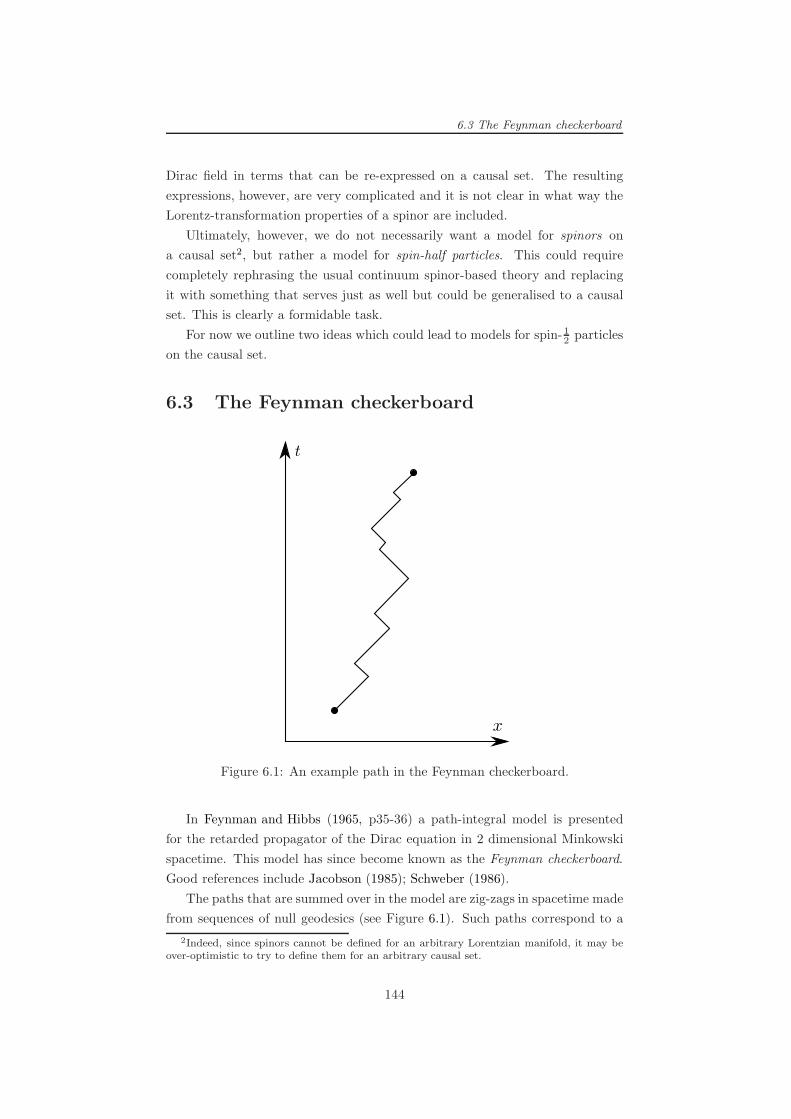
6.3 The Feynman checkerboard
Dirac field in terms that can be re-expressed on a causal set. The resulting
expressions, however, are very complicated and it is not clear in what way the
Lorentz-transformation properties of a spinor are included.
Ultimately, however, we do not necessarily want a model for spinors on
a causal set2, but rather a model for spin-half particles. This could require
completely rephrasing the usual continuum spinor-based theory and replacing
it with something that serves just as well but could be generalised to a causal
set. This is clearly a formidable task.
For now we outline two ideas which could lead to models for spin- 12 particles
on the causal set.
6.3 The Feynman checkerboard
Figure 6.1: An example path in the Feynman checkerboard.
In Feynman and Hibbs (1965, p35-36) a path-integral model is presented
for the retarded propagator of the Dirac equation in 2 dimensional Minkowski
spacetime. This model has since become known as the Feynman checkerboard.
Good references include Jacobson (1985); Schweber (1986).
The paths that are summed over in the model are zig-zags in spacetime made
from sequences of null geodesics (see Figure 6.1). Such paths correspond to a
2Indeed, since spinors cannot be defined for an arbitrary Lorentzian manifold, it may beover-optimistic to try to define them for an arbitrary causal set.
144

6.3 The Feynman checkerboard
particle shuttling forward and backward (along the one spatial dimension) at
the speed of light.
The sum-over-paths is calculated by discretising the time variable. If time
is discretised to progress in steps of size ǫ we can restrict the sum to the finite
number of paths which have zig-zag corners at times nǫ where n is an integer
(this restricts the class of paths to those that lie on a lightcone-lattice). After
calculating this finite sum we can then take the continuum limit as ǫ tends to
0. Each corner in the zig-zag path corresponds to a reversal of the direction the
particle is travelling in (for example the path in Figure 6.1 has 10 corners).
The amplitude assigned to a path with R corners (i.e. R reversals of direc-
tion) is then (imǫ)R where m is the mass of the particle.
Feynman and Hibbs left it to the reader to show that this path integral model
correctly reproduces the retarded Dirac propagator in M2 (detailed solutions
showing this appear in Jacobson and Schulman (1984) and Kull and Treumann
(1999)).
The method of solution involves representing the Dirac propagator in M2 as
a 2× 2 matrix depending on position. If we label its elements as
K(x) =
(K++(x) K+−(x)
K−+(x) K−−(x)
), (6.4)
then in the checkerboard model K++(x − y) is the amplitude that the parti-
cle started at x with positive velocity and arrived at y with positive velocity,
K+−(x−y) is the amplitude that the particle started at x with positive velocity
and arrived at y with negative velocity, with similar expressions for K−+(x− y)and K−−(x− y). In particular the amplitudes K++ and K−− (resp. K+− and
K−+) involve summing over paths with an even (resp. odd) number of corners.
Generalising the model to 3+1 dimensions was attempted by Feynman but
not published (Schweber, 1986) and has been attempted by subsequent authors
(including Jacobson and Schulman (1984); Jacobson (1984) and others).
6.3.1 The checkerboard on a causal set
It is a natural step to attempt to formulate a checkerboard-type model for spin-12 particles on a causal set. Indeed, the zig-zag trajectories which are summed
over in the checkerboard model are reminiscent of the hop-and-stop path integral
model of Chapter 3.
The first task is to characterise the appropriate zig-zag trajectories on a
causal set. Since each straight segment in the original model is a null ray the
most naıve choice for the straight parts of the causal set trajectories would be
links. Each link is certainly a good candidate for a null segment of the trajectory
145

6.3 The Feynman checkerboard
but the difficulty comes when one tries to identify the number of corners for a
trajectory (or indeed where the corners are).
To see the difficulty it helps to look at the light-cone lattice that the contin-
uum checkerboard-model is formulated on. Treating this as a causal set we let
u ≺∗ v be a link in the light-cone lattice (see Figure 6.2). To continue the path
with another link we could choose the next element to be either w1 or w2.
Figure 6.2: A segment of the light-cone lattice drawn as a Hasse diagram.
We would want the path u ≺∗ v ≺∗w1 to count as having 1 corner but the
path u ≺∗ v ≺∗w2 to count as having 0 corners. To distinguish between these
two trajectories we need more information than is provided by just knowing
that the elements are linked.
We can make this distinction, for the light-cone lattice at least, by using the
idea of a chain interval. This is a subset of the causal set which is both a chain
and an interval, i.e. a causal interval which happens to be totally ordered. In the
continuum3 and on the light-cone lattice these are precisely the null-geodesics.
Every chain interval in a causal set is a path and, to be more explicit, a
chain interval of length n is a sequence of elements v0 ≺∗ v1 ≺∗ v2 . . . ≺∗ vn such
that the causal interval [v0, vn] is totally ordered. We will denote such a chain
interval by its interval: [v0, vn].
In translating the checkerboard model to the causal set we take the straight
parts of the trajectories to be chain intervals and the trajectories themselves
to be concatenations of chain intervals—that is, each trajectory is a sequence
of chain intervals joining two elements vx and vy related as [vx, v1], [v1, v2],
[v2, v3], . . . , [vn, vy]. Such a sequence is not unique and can always be lengthened
3See Levichev (1987, Lemma 2).
146

6.3 The Feynman checkerboard
by adding in extra copies of single-element chain intervals [vi, vi].
Each of these concatenations of chain intervals is a path. The sum-over-
trajectories, therefore, is really a sum over all paths joining two elements. This
is similar to the hop-and-stop model of Chapter 3, the main difference being in
the amplitude that is assigned to each path.
Corners
We can assign a non-negative integer R to a path in a causal set by using the
fact that every path can be re-expressed as a sequence of chain intervals. To
see this we simply realise that every link in the path is a chain interval but
acknowledge that there may be larger chain intervals in the path which contain
more than two elements.
We define the number of corners R of a path to be the minimum number of
chain intervals into which it can be resolved, minus one.
To illustrate this definition we return to Figure 6.2. Here [u, v] and [v, w1]
are both chain intervals but [u,w1] is not a chain interval (since it is not totally
ordered). Thus the path u ≺∗ v ≺∗w1 can be resolved into a minimum of two
chain intervals so is assigned 1 corner.
For the other path we have that [u, v] and [v, w2] are both chain intervals
but so is [u,w2]. Therefore u ≺∗ v ≺∗w2 can be resolved into one chain interval
so is assigned 0 corners.
Our definition of “number of corners” agrees with usual notion of corner
when applied to paths in the light-cone lattice. A slightly unsatisfactory aspect
to our definition, however, is that for a general causal set (in contrast to the
light-cone lattice) we may be unable to assign the corners to particular elements
in the path.
Consider, for example, Figure 6.3. The path P = u1 ≺∗ u2 ≺∗ u3 ≺∗ u4 ≺∗ u5 ≺∗ u6 is not a chain interval. It can be resolved, however, into two chain
intervals: [u1, u3], [u3, u6]. We therefore assign P one corner and, looking at the
resolution into chain intervals, we’d be tempted to assign the corner to u3.
This is wrong, however, because P can also be resolved as [u1, u4], [u4, u6].
From this resolution we would be tempted to assign the corner to u4. It is thus
clear that while our definition assigns one corner to P it does not assign it to
any particular element. In other words, we should not think of the corners as
being assigned to a particular element but rather that the “number of corners”
is a property of the path as a whole.
147

6.3 The Feynman checkerboard
Figure 6.3: Corners applied to a particular example.
6.3.2 The path integral
Having established which trajectories we shall sum over we now consider what
amplitudes we should assign to them.
The continuum Dirac propagator in M2 has mass-dimension M . We there-
fore want the amplitudes we assign to paths to have dimension M . Inspired by
the usual continuum checkerboard model as well as the hop-and-stop path inte-
gral of Chapter 3 we assume the amplitude assigned to a path with n corners is
an+1bn where a and b are appropriate constants (we think of each corner having
a “stop amplitude” b).
On dimensional grounds we have
[a] =M, [b] =M−1, [ab] = 1, (6.5)
and if our causal set is generated by a sprinkling into M2 with density ρ the
only dimensionful quantities available are ρ and m:
[ρ] =M2, [m] =M. (6.6)
Therefore, in a similar spirit to the 1+1 dimensional scalar path integral of
Section 3.6, we take
a = A√ρ, b = B
m
ρ, (6.7)
where A and B are dimensionless (possibly complex) constants independent of
ρ or m.
To compute the sum-over-paths on a p-element causal set we can define a
148

6.4 Square root of the propagator
family of p× p matrices T (n) (n = 0, 1, 2, . . .) as:
T (n)xy := The number of paths from vx to vy with n corners. (6.8)
Calculating these matrices explicitly is difficult but we mention that
T (0)xy :=
1 if [vx, vy] is a chain interval
0 otherwise.(6.9)
can be computed from the causal matrix C as:
T (0)xy =
(I + C(1+(C2)xy)
)
xy, (6.10)
where I is the p×p identity matrix. This follows because if [vx, vy] is a chain in-
terval and vx ≺ vy then there is exactly 1 chain of length 1+(C2)xy = |[vx, vy]|−1
from vx to vy. If [vx, vy] is not a chain interval then(C(1+(C2)xy)
)
xy= 0 since
there are no chains of length 1 + (C2)xy from vx to vy.
The 4-elements of the propagator K++,K+−,K−+,K−− would then be cal-
culated as
K++ = K−− = aT (0) + a32T (2) + a5b4T (4) + . . . =∑
n even
an+1bnT (n), (6.11)
K+− = K−+ = a2bT (1) + a4b3T (3) + a6b5T (5) + . . . =∑
n odd
an+1bnT (n),
(6.12)
where we sum over odd or even numbers of corners in the same way as the usual
checkerboard model.
By further analysing this model for causal sets generated by sprinkling into
M2 it is possible that we could choose the A and B constants to give a good
model for the Dirac propagator.
6.4 Square root of the propagator
An alternative approach to modelling spin- 12 particles attempts to replicate
Dirac’s insight that by “taking a suitable square-root” of the Klein-Gordon
equation we can obtain the Dirac equation.
The insight is that the Klein-Gordon operator can be factorised as:
+m2 = (−iγµ∂µ −m)(iγν∂ν −m). (6.3)
To use this we now consider the retarded propagator for the Dirac equation,
149

6.4 Square root of the propagator
which we’ll denote by Rm(x), which satisfies:
(iγµ∂µ −m)Rm(x) = δ(x)I. (6.13)
Here Rm(x) is a matrix-valued function of position and I is an identity matrix
the same size as the Dirac matrices.
If we now define the matrix-valued function
Sm(x − y) := −∫ddzRm(x− z)R−m(z − y), (6.14)
then we have that
(+m2)Sm(x− y) = (iγµ∂µ +m)(iγν∂ν −m)
∫ddzRm(x− z)R−m(z − y),
(6.15)
= (iγµ∂µ +m)
∫ddz ((iγν∂ν −m)Rm(x− z))R−m(z − y),
(6.16)
= (iγµ∂µ +m)R−m(x− y) = δ(x− y)I. (6.17)
This means that the diagonal of the matrix-valued function Sm(x) is a propaga-
tor for the Klein-Gordon equation. Since Rm(x) is retarded so is Sm(x) which
means that the diagonal of Sm(x) must be the retarded Klein-Gordon propaga-
tor (which is the unique retarded propagator for the Klein-Gordon equation).
The off-diagonal entries of Sm(x) are retarded solutions of the Klein-Gordon
equation (i.e. they are zero).
This observation suggests that we can obtain the retarded Dirac propagator
as the square-root of the retarded Klein-Gordon propagator.
To implement this on a causal set with p elements we seek a square matrix
Rm such that
− 1
ρRmR−m = KR ⊗ I, (6.18)
or
RmR−m = −ρKR ⊗ I, (6.19)
where KR is the retarded propagator on the causal set obtained from Chapter
3 and we have included a factor of ρ to mirror the dimensionful integration in
(6.14). This ensures that the Rm has the correct mass dimension of Md−1.
The size of the identity matrix I corresponds to the size of the “spin-space”
for the particles. In turn this depends on which dimension we are working in
and whether we are using the 4-spinor or 2-spinor theory (e.g. for the 4-spinor
theory in d = 4, I would be a 4 × 4 matrix). Ideally, we would like the size of
150

6.5 General approach
this spin-space to be determined by the act of taking the square root of KR, i.e.
we’d like it to only work for I of a particular size. This would be similar to the
way in which (6.3) only holds for Dirac matrices of a particular size.
6.4.1 Mass scattering
The square-root of the propagator is consistent with the mass scattering ideas
from Section 3.9. To see this we follow the results from Chapter 3 and suppose
that the retarded Klein-Gordon propagator takes the form
KR = Φ
(I +
m2
ρΦ
)−1
, (6.20)
(where Φ is the matrix of “hop” amplitudes).
For the m = 0 case of (6.19) we then have
(R0)2 = −ρΦ⊗ I. (6.21)
If we now define a “mass scattering series”
Rm = R0 + b(R0)2 + b2(R0)
3 + . . . = R0(I − bR0)−1, (6.22)
(where we suppose b is a mass-dependent amplitude such that if m is replaced
by −m then b becomes −b) then the product RmR−m is:
RmR−m = R0(I − bR0)−1(I + bR0)
−1R0 = R20(I − b2(R0)
2)−1 (6.23)
= −ρ(Φ⊗ I)(I + b2ρΦ⊗ I
)−1= −ρ
(Φ(I + b2ρΦ)−1
)⊗ I. (6.24)
This is equal to −ρ (KR ⊗ I) if b2ρ = m2/ρ, i.e. b = ±mρ .
We see, therefore, that if we determine R0 we can obtain Rm through the
series (6.22). The b amplitude is the same form as the b amplitude in (6.7).
This may suggest that the checkerboard and square-root models take the same
form in M2.
The square roots of a matrix (if they exist) are in general not unique. It is
possible that further conditions must be imposed to define the correct square
root of −ρKR ⊗ I to serve as the retarded Dirac propagator. This remains a
task for future work.
6.5 General approach
We have only been able to present a few suggestions for obtaining the retarded
propagator for the Dirac equation on a causal set. Nevertheless here we outline
151
6.5 General approach
how one would proceed if we had obtained the propagator.
To model a spin- 12 particle on a causal set we would expect to require a multi-
component field ψαx (where α = 1, . . . , S denotes the spin degrees of freedom
and x = 1, . . . , p indexes the causal set elements vx).
Now suppose the retarded propagator is (KR)αx,βy (which, if we treat αx and
βy as single indices, we can think of as a pS × pS matrix). This represents the
amplitude that a particle at vx propagates to vy (with spin degrees-of-freedom
described by the α and β indices).
The Pauli-Jordan function would then be
∆αx,βy = (KR)αx,βy − (KR)βy,αx. (6.25)
Since these would represent fermionic fields we would expect to quantize
them with anti-commutation relations along the lines of4:
ψαx, ψ†βy = i∆αx,βy, (6.26)
where A, B := AB + BA is the anticommutator.
The eigendecomposition of i∆ could then be used to express the ψ operators
as linear combinations of anticommuting creation and annihilation operators
acting on a fermionic Fock space (see Geroch (1985, Chapter 21)). Together
with a suitable analogue of condition 3 (4.35) this might be sufficient to define
a free field theory for spin- 12 particles on a causal set.
4We use the adjoint ψ† but this may need to be replaced by an analogue of the Diracadjoint ψ = ψ†γ0 used in the continuum theory.
152

Chapter 7
Conclusions
We conclude by summarising the work presented and discussing directions for
future work.
7.1 Summary
Chapter 1 gave an overview of the motivations for causal set theory, including
the problem of quantum gravity as well as difficulties with continuum models for
spacetime. Chapter 2 introduced causal set theory in detail, including definitions
and an overview of current developments.
In Chapter 3 we presented a model for discrete path integrals on a causal set.
For a suitable choice of parameters (and when evaluated on causal sets generated
by sprinkling into d-dimensional Minkowski spacetime) these give agreement
with the continuum retarded propagator for the Klein-Gordon equation in d-
dimensional Minkowski spacetime (for d = 1, 2, 3, 4). Variations on the models
as well as possible extensions were discussed.
The path integrals of Chapter 3 were used as the starting-point for Chapter
4. Here we defined a model for free quantum scalar field theory on a causal
set. This was done by assigning each causal set element a field operator, the
collection of which were subject to three simple conditions. These operators
were then used to define a Feynman propagator on a causal set (as the vacuum
expectation value of a time-ordered product of field operators). The formal
properties of this model were discussed and evidence for the agreement between
the Feynman propagator on the causal set and the Feynman propagator in
Minkowski spacetime was presented. The method for obtaining the Feynman
propagator was also applied to calculations in the continuum.
In Chapter 5 the free quantum scalar field theory was extended to include in-
teracting scalar fields. This included defining a causal set analogue of the Dyson
153

7.2 Directions for future work
series for the S-matrix. This was then used to motivate a non-perturbative def-
inition of the S-matrix on a causal set. Discussion of how this framework could
be used was also given.
In Chapter 6 two speculative suggestions were given for how to model spin-
half particles on a causal set. One of these involved translating the Feynman
checkerboard model to a causal set.
7.2 Directions for future work
The current work opens up a number of areas for future study. Firstly we would
like to better understand the models already presented, including:
• Calculating the expectation values of the retarded and Feynman propaga-
tors for finite ρ in d-dimensional Minkowski spacetime (including, at least,
the physical d = 4 case).
• Calculating the variance of the causal set propagators and investigating
how the variance behaves in the ρ→ ∞ limit.
• Investigating the behaviour of the propagators for sprinklings into curved
spacetimes.
• Investigating the convergence of the perturbative causal set Dyson series.
• Better understanding the non-perturbative S-matrix (for example, calcu-
lating its matrix elements).
• Better understanding how the framework can be extended from finite to
infinite causal sets.
• Applying the interacting theory to massless scalar fields with an interac-
tion term Hx = m2
ρ φ2x to see if we recover free massive scalar field theory.
If we better understood the expectation values of the causal set propagators
then we could follow the phenomenological approach described in Section 5.9 to
get a causal-set inspired model for a realistic field theory.
Extending the work presented here from scalar fields to realistic interacting
matter fields would represent the conclusion of the ideas developed so far. If we
had, for example, the Standard Model on a causal set then we could calculate
experimentally measurable quantities within the causal set framework. These
calculations would have a dependence on the fundamental spacetime volume for
each causal set element. Comparing the calculations with experimental results
would provide evidence on whether spacetime is discrete and, if it is, what the
154

7.2 Directions for future work
discreteness scale is. To achieve this goal there are (at least) two key tasks to
do:
• Developing a theory of spin-half and spin-one particles on a causal set.
• Better understanding physical quantities such as energy, momentum and
angular momentum on a causal set.
If these tasks can be completed then we would have a realistic theory of matter
on a causal set spacetime background!
155

Appendix A
Expected Number of Paths
In Section 3.5.2 we discussed calculating the expected number of paths of length
n between two points in a sprinkling into d-dimensional Minkowski spacetime.
No analytic expression is yet known for this quantity for general values of d and
n but here we present some approaches to the problem.
A.1 Preliminaries
We first describe the quantity we are trying to calculate. We start by fixing two
points x, y ∈ Md. We then sprinkle a causal set with density ρ into Md. There
is zero probability that the sprinkled causal set will contain x and y so we add
them to the causal set. We now count the number of paths within the causal
set of length n from x to y (now regarded as elements of the causal set). The
number we get is then averaged over all sprinklings with the same density ρ to
give us a density-dependent function Pn(y − x). Our goal is to determine this
function as fully as possible.
Before we begin we fix some notation. For two functions f, g on Md their
convolution is defined as:
(f ∗ g)(x) :=∫ddyf(x− y)g(y). (A.1)
We define two useful functions (which we met earlier in Section 3.5.1 and Section
3.5.2):
C(y − x) :=
1 if x y
0 otherwise,(A.2)
P (y − x) := C(y − x)e−ρV (x−y) =
e−ρV (x−y) if x y
0 otherwise,(A.3)
156
A.1 Preliminaries
where V (x− y) is the d-dimensional Minkowski spacetime volume of the causal
interval between x and y (see (3.28)).
As discussed in Section 3.5.1, the expected number of chains of length one
from x to y is C1(y − x) := C(y − x). The expected number of chains of length
n > 1 from x to y is given by
Cn(y − x) := ρ(C ∗ Cn−1)(y − x) = ρn−1(C ∗ C ∗ . . . ∗ C)(y − x), (A.4)
where there are n copies of C and n− 1 convolutions in the final expression.
From the definition we have:
ρCn ∗ Cm = Cn+m. (A.5)
As discussed in 3.5.2, the expected number of paths of length one from x to
y is given by P1(y − x) := P (y − x). The expected number of paths of length
n > 1 from x to y is given:
Pn(y − x) := ρ(P ∗ Pn−1)(y − x) = ρn−1(P ∗ P ∗ . . . ∗ P )(y − x), (A.6)
where there are n copies of P and n− 1 convolutions.
The expression for Cn(x− y) has been calculated explicitly by Meyer (1988,
Theorem III.2, p50). For n ≥ 1 we have:
Cn(y − x) = C(y − x)(ρV (x− y))n−1Dn, (A.7)
where D1 := 1 and
Dn :=1
n− 1
(Γ(d+ 1)
2
)(n−2)Γ(ω)Γ(2ω)
Γ((n− 1)ω)Γ(nω), (A.8)
for n > 1 is a real dimensionless constant with ω = d/2. We have D2 = 1 in all
dimensions.
Using these expressions the expected total number of chains is CT (y − x):
CT (y − x) :=
∞∑
n=1
Cn(y − x) (A.9)
=C(y − x) 0Fd−1
(( )
2kd , k = 1, . . . , d− 1
∣∣∣∣∣Γ(d)(d2
)d−1ρV
), (A.10)
where 0Fd−1 is a generalised hypergeometric function.
157

A.2 Convolution approach
For particular values of d this simplifies. For example in d = 2 we have:
CT (y − x) = C(y − x) 0F1
(( )
1
∣∣∣∣∣ ρV)
= I0(2√ρV ), (A.11)
and in d = 4 we have
CT (y − x) = C(y − x) 0F3
(( )
12 ,
22 ,
32
∣∣∣∣∣3
4ρV
)=
1
z(I1(z) + J1(z)) , (A.12)
where z = 2(12ρV )14 (compare to (3.60) in Section 3.7).
A.2 Convolution approach
One approach to determining the Pn functions involves expanding P (x) in terms
of the functions Cn(x) to give:
P (x) = C(x)e−ρV (x) = C(x)
∞∑
n=0
(−ρV (x))n
n!=
∞∑
n=0
(−1)nCn+1(x)
n!Dn+1, (A.13)
where we have used (A.7).
In this form we can use (A.5) to compute expressions for Pn As an example
we have
P2 := ρP ∗ P =
∞∑
n=0
∞∑
m=0
(−1)n+mρCn+1 ∗ Cm+1
n!m!Dn+1Dm+1=
∞∑
n=0
∞∑
m=0
(−1)n+mCn+m+2
n!m!Dn+1Dm+1
(A.14)
=
∞∑
n=0
∞∑
m=0
(−1)n+mC(ρV )n+m+1Dn+m+2
n!m!Dn+1Dm+1, (A.15)
where we have used (A.5) and (A.7).
By resumming the terms in this series we can replace the double infinite
summation by one infinite and one finite summation to give
P2 =
∞∑
n=0
n∑
k=0
(−1)nCn+2
k!(n− k)!Dk+1Dn−k+1=
∞∑
n=0
n∑
k=0
(−1)nC(ρV )n+1Dn+2
k!(n− k)!Dk+1Dn−k+1.
(A.16)
In fact this procedure can be performed for general Pn. In effect we treat P
as a formal power series in a variable C where the nth “power” of the variable
is Cn (i.e. the “product” of two functions f and g is ρf ∗ g).We can use the following result (Gradshteyn and Ryzhik, 1965, 0.314, p14)
158

A.2 Convolution approach
that: ( ∞∑
k=0
akxk
)n=
∞∑
k=0
ckxk, (A.17)
with
c0 = an0 , cm =1
ma0
m∑
k=1
(kn−m+ k)akcn−k. (A.18)
Applying this to (A.13) we have, for n ≥ 1,
Pn =
∞∑
m=0
gmCm+n =
∞∑
m=0
gmDm+nC(ρV )n+m−1, (A.19)
where the gm coefficients satisfy the recurrence relation
g0 = 1 gm =1
m
m∑
k=1
(k(n+ 1)−m)(−1)k
k!Dk+1gm−k. (A.20)
As an example, for d = 2 we have (for causally related points)
P1 = 1− z +z2
2− z3
6+z4
24− z5
120+
z6
720+O
(z7)
(A.21)
P2 = z − z2
2+
5z3
36− z4
36+
z5
225− 13z6
21600+
151z7
2116800+O
(z8)
(A.22)
P3 =z2
4− z3
12+z4
64− 31z5
14400+
7z6
28800− 101z7
4233600+
857z8
406425600+O
(z9)
(A.23)
P4 =z3
36− z4
144+
7z5
7200− 13z6
129600+
31z7
3628800− 13z8
20321280+O
(z9)
(A.24)
where z = ρV .
A.2.1 Total number of paths
We are also interested in the expected total number of paths from x to y. Calling
this PT we have
PT (y − x) :=∞∑
n=1
Pn(y − x). (A.25)
Treating this as a formal power series in P (again, with the nth “power” of the
P equal to Pn) we have
PT =P
1− P. (A.26)
We can now use the expression for P as a formal power series in C and use
159
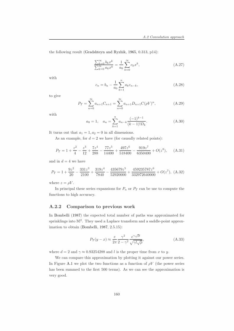
A.2 Convolution approach
the following result (Gradshteyn and Ryzhik, 1965, 0.313, p14):
∑∞k=0 bkx
k
∑∞k=0 akx
k=
1
a0
∞∑
k=0
ckxk, (A.27)
with
cn = bn − 1
a0
n∑
k=1
akcn−k, (A.28)
to give
PT =∞∑
n=0
an+1Cn+1 =∞∑
n=0
an+1Dn+1C(ρV )n, (A.29)
with
a0 = 1, an =
n∑
k=1
an−k(−1)k−1
(k − 1)!Dk. (A.30)
It turns out that a1 = 1, a2 = 0 in all dimensions.
As an example, for d = 2 we have (for causally related points):
PT = 1 +z2
4− z3
12+
7z4
288− 77z5
14400+
497z6
518400− 919z7
6350400+O(z8), (A.31)
and in d = 4 we have
PT = 1+9z2
20− 331z3
2100+
319z4
7840− 435679z5
52920000+
459235787z6
332972640000+O(z7), (A.32)
where z = ρV .
In principal these series expansions for Pn or PT can be use to compute the
functions to high accuracy.
A.2.2 Comparison to previous work
In Bombelli (1987) the expected total number of paths was approximated for
sprinklings into M2. They used a Laplace transform and a saddle-point approx-
imation to obtain (Bombelli, 1987, 2.5.15):
PT (y − x) ≈ e
2π
γ2
2− γ2eγ
√ρl
√γl√ρ, (A.33)
where d = 2 and γ ≈ 0.93254288 and l is the proper time from x to y.
We can compare this approximation by plotting it against our power series.
In Figure A.1 we plot the two functions as a function of ρV (the power series
has been summed to the first 500 terms). As we can see the approximation is
very good.
160

A.2 Convolution approach
Figure A.1: Comparison of the power series for PT and Bombelli’s approxima-tion (A.33).
A.2.3 Comparison to total number of chains
Since every path is a chain the total number of paths is always less than the
total number of chains. Here we plot the power series for PT against the total
number of chains (A.12) for d = 2 and d = 4 dimensions.
Two dimensions
Figure A.2: Comparison of the expected total number of chains and paths forsprinklings into two dimensional Minkowski spacetime.
161

A.3 Green’s function approach
From Figure A.2 we see that in the d = 2 case the vast majority of chains
are not paths.
Four dimensions
Figure A.3: Comparison of the expected total number of chains and paths forsprinklings into four dimensional Minkowski spacetime.
From Figure A.3 we see that in the d = 4 case around half of all chains are
paths.
A.3 Green’s function approach
Another approach to determining Pn is to try to find a differential equation
satisfied by the Pn and PT functions.
We start with the observation that1 (Bollini and Giambiagi, 1993, eq 22 with
α = d/2)
d/2C(x) = Aδ(x), (A.34)
where δ is the d-dimensional delta-function, = ∂2x0 − ∂2~x is the d’Alembertian
and A is a constant equal to
A = 2d−1πd/2−1Γ(d/2). (A.35)
1Fractional powers of are defined through the Fourier transform.
162

A.3 Green’s function approach
From this and (A.4) we have
d/2Cn = ρ
(
d/2C)∗ Cn−1 = Aρδ ∗ Cn−1 = AρCn−1. (A.36)
Recalling that
P (x) = C(x)e−ρV (x) = C(x)∞∑
n=0
(−ρV (x))n
n!=
∞∑
n=0
(−1)nCn+1(x)
n!Dn+1, (A.13)
it immediately follows that
d/2P = Aδ +Aρ
∞∑
n=1
(−1)nCn
n!Dn+1= Aδ +AρC
∞∑
n=1
(−1)n(ρV )n−1Dn
n!Dn+1. (A.37)
This infinite sum can be evaluated and is equal to
C
∞∑
n=1
(−1)n(ρV )n−1Dn
n!Dn+1= − 1
(d− 1)!
(d
2H+1
)(d
2H+2
)· · ·(d
2H+d−1
)P,
(A.38)
where H = ρ ∂∂ρ is a differential operator. We can see this holds by expanding
both sides in powers of ρV .
In 1+1 dimensions we have:
C∞∑
n=1
(−1)n(ρV )n−1Dn
n!Dn+1= (−1 + ρV )P = −(H + 1)P. (A.39)
In 3+1 dimensions we have
C
∞∑
n=1
(−1)n(ρV )n−1Dn
n!Dn+1= (−1 + 9ρV − 8(ρV )2 +
4
3(ρV )3)P (A.40)
= −1
6(2H + 1)(2H + 2)(2H + 3)P. (A.41)
We now specialise to the two and four-dimensional cases.
A.3.1 1+1 dimensions
In 1+1 dimensions we have
C = 2δ, (A.42)
which leads to
P = 2δ + 2ρ(−1 + ρV )P, (A.43)
or
(+ 2ρ(1− ρV ))P = (+ 2ρ (H + 1))P = 2δ. (A.44)
163

A.3 Green’s function approach
Now for n > 1 we have Pn = ρn−1P ∗ P ∗ · · · ∗ P (with n copies of P ). This
means that2
HPn = (n− 1)Pn + ρn−1[(HP ) ∗ P ∗ · · · ∗ P (A.45)
+ P ∗ (HP ) ∗ P ∗ · · · ∗ P + . . .+ P ∗ · · · ∗ P ∗ (HP )] (A.46)
= (n− 1)Pn + nρ(HP ) ∗ Pn−1, (A.47)
or
(H + 1)Pn = nρ((H + 1)P ) ∗ Pn−1. (A.48)
Therefore
Pn = ρ(P ) ∗ Pn−1 = ρ(2δ + 2ρ(H + 1)P ) ∗ Pn−1 (A.49)
= 2ρPn−1 −2
nρ(H + 1)Pn, (A.50)
or (+
2
nρ
(1 + ρ
∂
∂ρ
))Pn = 2ρPn−1. (A.51)
This partial differential equation for Pn could, in principle, be solved one n at
a time starting with n = 2.
Total number of paths
It’s helpful to define the generating function for the expected number of paths:
PT (z) :=
∞∑
n=1
zn−1Pn = P1 + zP2 + z2P3 + . . . , (A.52)
for some real number z. Note that PT (1) is the expected total number of paths.
Using (A.44) and (A.50) we have
(H + 1)P1 =δ
ρ−
2ρP1, (H + 1)Pn = n
(Pn−1 −
2ρPn
). (A.53)
Using these and applying H + 1 term-by-term to PT gives:
(H+1)PT =
(δ
ρ−
2ρP1
)+2z
(P1 −
2ρP2
)+3z2
(P2 −
2ρP3
)+. . . , (A.54)
2H(c(f ∗ g)) = (Hc)(f ∗ g) + c(Hf) ∗ g + cf ∗ (Hg)
164

A.3 Green’s function approach
or
(H + 1)PT =δ
ρ+(2zP1 + 3z2P2 + . . .
)−
2ρ
(P1 + 2zP2 + 3z2P3 + . . .
)
(A.55)
=δ
ρ+
∂
∂z(z2PT )−
2ρ
∂
∂z(zPT ). (A.56)
We have therefore obtained a partial differential equation satisfied by PT (z),
namely:
ρ∂PT
∂ρ+ PT − ∂
∂z(z2PT ) +
2ρ
∂
∂z(zPT ) =
δ
ρ, (A.57)
with the boundary condition that PT (0) = P1. If this could be solved we would
be able to determine PT (z).
A.3.2 3+1 dimensions
In four dimensions we have
2C = 8πδ. (A.58)
This gives
2P = 8πδ + 8πρP
(−1 + 8(ρV )− 9(ρV )2 +
4
3(ρV )3
), (A.59)
= 8πδ − 8πρ1
6(2H + 1)(2H + 2)(2H + 3)P. (A.60)
Due to the complexity of this differential equation we will not attempt to derive
differential equations satisfied by general Pn or PT .
Nevertheless, we mention that this equation provides a surprising link with
the causal set d’Alembertian work of Benincasa and Dowker (2010). In that
work they show that the expected value of the causal set d’Alembertian (applied
to a field φ and evaluated at a point x ∈ M4) is (B ∗φ)(x) for a suitable integral
kernel B(x). As it turns out we have
2P =
2π√6√ρB, (A.61)
(compare with Benincasa and Dowker (2010, eq. (4))). Defining KR :=√ρ
2π√6P
then we have
2KR = B. (A.62)
But KR is the expected value of the 4 dimensional massless retarded propagator
defined in Section 3.7! This surprising connection shows that the current work
165

A.3 Green’s function approach
and the work of Benincasa and Dowker are mutually consistent. We can see
this by evaluating B ∗ φ and taking the infinite density limit:
B ∗ φ = (2KR) ∗ φ = (KR) ∗ (φ). (A.63)
The work of Section 3.7 showed that in the infinite density limit we have
limρ→∞
KR = δ, (A.64)
which means that
limρ→∞
B ∗ φ = limρ→∞
(KR) ∗ (φ) = δ ∗ (φ) = φ, (A.65)
as was shown by other means by Benincasa and Dowker (2010).
166

Bibliography
Abramowitz, M. and Stegun, I.: 1965, Handbook of Mathematical Functions, Dover
Publications, New York.
Ahmed, M. and Rideout, D. P.: 2009, Indications of de Sitter Spacetime from Classical
Sequential Growth Dynamics of Causal Sets. arXiv:0909.4771.
Amsler, C. et al.: 2008, Review of particle physics, Phys. Lett. B667, 1.
Aste, A.: 2007, Resummation of mass terms in perturbative massless quantum field
theory, Lett. Math. Phys. 81, 77–92. arXiv:hep-th/0703120.
Benincasa, D. M. T. and Dowker, F.: 2010, The Scalar Curvature of a Causal Set.
arXiv:1001.2725.
Birrell, N. D. and Davies, P.: 1982, Quantum Fields In Curves Space, Cambridge
University Press.
Bogoliubov, N. N. and Shirkov, D. V.: 1959, Introduction to the theory of quantized
fields, Vol. 3 of Intersci. Monogr. Phys. Astron., Interscience, New York.
Bollini, C. G. and Giambiagi, J. J.: 1993, Arbitrary powers of D’Alembertians and
the Huygens’ principle, J. Math. Phys. 34, 610–621.
Bombelli, L.: 1987, Space–time as a casual set, PhD thesis, Syracuse University.
Bombelli, L., Lee, J.-H., Meyer, D. and Sorkin, R. D.: 1987, Space-Time as a Causal
Set, Phys. Rev. Lett. 59, 521.
Bombelli, L. and Sonego, S.: 1994, Relationships between various characterizations of
wave tails, J. Phys. A27, 7177–7199.
Bratteli, O. and Robinson, D.: 1981, Operator Algebras and Quantum Statistical Me-
chanics II, Springer-Verlag, New York.
Champeney, D. C.: 1989, A handbook of Fourier theorems, Cambridge University
Press, Cambridge.
Contaldi, C., Dowker, F. and Philpott, L.: 2010, Polarization Diffusion from Spacetime
Uncertainty. arXiv:1001.4545.
Daughton, A.: 1993, The Recovery of Locality for Causal Sets and Related Topics,
PhD thesis, Syracuse University.
De Jager, E.M.: 1967, The lorentz-invariant solutions of the klein-gordon equation,
SIAM Journal on Applied Mathematics 15(4), 944–963.
DeWitt, B.: 2009, Quantum Gravity Yesterday and Today, Gen. Rel. Grav. 41, 413–
167

419. arXiv:0805.2935.
Dirac, P. A. M.: 1933, The Lagrangian in quantum mechanics, Phys. Z. Sowjetunion
3, 64–72.
Dorf, R.: 1997, The electrical engineering handbook, CRC Press.
Dowker, F.: 2005, Causal sets and the deep structure of spacetime. arXiv:gr-
qc/0508109.
Dowker, F.: 2006, Causal sets as discrete spacetime, Contemp. Phys. 47, 1–9.
Dowker, F., Henson, J. and Sorkin, R. D.: 2004, Quantum gravity phenomenology,
Lorentz invariance and discreteness, Mod. Phys. Lett. A19, 1829–1840. arXiv:gr-
qc/0311055.
Dowker, F., Johnston, S. and Surya, S.: 2010, On extending the Quantum Measure.
arXiv:1007.2725.
Dugne, J. J. and Karmanov, V. A.: 2003, Spin zero particle propagator from a random
walk in 3-D space, Phys. Lett. A310, 131–138. arXiv:hep-th/0303028.
Egorov, Y. and Shubin, M. (eds): 1994, Partial Differential Equations II, Springer-
Verlag.
Feynman, R. P.: 1948a, A relativistic cut-off for classical electrodynamics, Phys. Rev.
74, 939–946.
Feynman, R. P.: 1948b, Relativistic cutoff for quantum electrodynamics, Phys. Rev.
74, 1430–1438.
Feynman, R. P.: 1948c, Space-time approach to nonrelativistic quantum mechanics,
Rev. Mod. Phys. 20, 367–387.
Feynman, R. P.: 1985, QED: The Strange Theory of Light and Matter, Penguin.
Feynman, R. P.: 2000, Closed loop and tree diagrams, in: Selected papers of Richard
Feynman: With commentary, World Scientific, Singapore.
Feynman, R. P. and Hibbs, A.: 1965, Quantum Mechanics and Path Integrals,
McGraw-Hill.
Follard, G. B.: 1989, Harmonic Analysis in Phase Space, Annals of Mathematics
Studies, Princeton University Press, Princeton, NJ.
Fulling, S. A.: 1989, Aspected of Quantum Field Theory in Curved Space-Time, Lon-
don Math. Soc. Student Texts 17, 1–315.
Gel’fand, I. and Shilov, G.: 1964, Generalized Functions, Academic Press.
Geroch, R.: 1973-74, Special Topics in Particle Physics. University of Chicago Lecture
Notes.
Geroch, R.: 1985, Mathematical physics, University of Chicago Press.
Gradshteyn, I. and Ryzhik, I.: 1965, Table of Integrals, Series, and Products, Academic
Press, New York.
Gudder, S.: 1988, Quantum Probability, Academic Press, New York.
Hawking, S. W. and Ellis, G. F. R.: 1973, The large scale structure of space-time,
Cambridge University Press.
168

Hawking, S. W., King, A. R. and McCarthy, P. J.: 1976, A New Topology for Curved
Space-Time Which Incorporates the Causal, Differential, and Conformal Structures,
J. Math. Phys. 17, 174–181.
Hemion, G.: 1980, A Quantum Theory of Space and Time, Found. Phys. 10, 819–840.
Hemion, G.: 1988, A discrete geometry: Speculations on a new framework for classical
electrodynamics, International Journal of Theoretical Physics 27(10), 1145–1255.
Henson, J.: 2006, The causal set approach to quantum gravity. arXiv:gr-qc/0601121.
Hoyle, F. and Narlikar, J. V.: 1974, Action-at-a-Distance in Physics and Cosmology,
W. H. Freeman, San Francisco.
Hustler, N.: 2010, Rindler space and causal sets, Master’s thesis, Imperial College
London, London.
Jacobson, T.: 1984, Spinor chain path integral for the Dirac electron, J. Phys.
A17, 2433.
Jacobson, T.: 1985, Feynman’s checkerboard and other games, Non-Linear Equations
in Classical and Quantum Field Theory 226, 386–395.
Jacobson, T. and Schulman, L. S.: 1984, Quantum Stochastics: The passage from a
relativistic to a nonrelativistic path integral, J. Phys. A17, 375.
Jauch, J. and Rohrlich, F.: 1955, The Theory of Photons and Electrons, Addison-
Wesley, Cambridge, MA.
Johnston, S.: 2008a, Particle propagators on discrete spacetime, Class. Quant. Grav.
25, 202001. arXiv:0806.3083.
Johnston, S.: 2008b, Path integrals on causal sets, Wolfram Demonstrations Project.
URL: http://demonstrations.wolfram.com/PathIntegralsOnCausalSets/
Johnston, S.: 2009a, Feynman Propagator for a Free Scalar Field on a Causal Set,
Phys. Rev. Lett. 103, 180401. arXiv:0909.0944.
Johnston, S.: 2009b, Path integrals on causal sets, J. Phys.: Conf. Ser. 174(012046).
Jordan, T.: 1969, Linear Operators for Quantum Mechanics, John Wiley & Sons.
Kaiser, D.: 2000, Stick-Figure Realism: Conventions, Reification, and the Persistence
of Feynman Diagrams, 1949-1964, Representations (70), 49–86.
Klauder, J. (ed.): 1972, Magic Without Magic, W.H. Freeman, San Francisco.
Kragh, H. S.: 1992, Dirac: A Scientific Biography, Cambridge University Press, Cam-
bridge.
Kull, A. and Treumann, R. A.: 1999, On the path integral of the relativistic electron,
Int. J. Theor. Phys. 38, 1423–1428. arXiv:quant-ph/9901058.
Levichev, A. V.: 1987, Prescribing the conformal geometry of a lorentz manifold by
means of its causal structure, Soviet Math. Dokl. 35, 452–455.
Major, S., Rideout, D. and Surya, S.: 2007, On recovering continuum topology from
a causal set, J. Math. Phys. 48, 032501. arXiv:gr-qc/0604124.
Malament, D.: 1977, The class of continuous timelike curves determines the topology
of spacetime, Journal of Mathematical Physics 18(7), 1399–1404.
169
Mehra, J. and Rechenberg, H.: 2000, The Historical Development of Quantum Theory,
Vol 6, Part 1, Springer-Verlag, New York.
Meyer, D.: 1988, The Dimension of Causal Sets, PhD thesis, M.I.T.
Meyer, D.: 1997, Causal Sets and Feynman diagrams. Talk presented at “New Direc-
tions in Simplicial Quantum Gravity”, July 28 - August 8, 1997.
Minguzzi, E. and Sanchez, M.: 2006, The causal hierarchy of spacetimes, in H. Baum
and D. Alekseevsky (eds), Recent developments in pseudo-Riemannian geometry,
ESI Lect. Math. Phys., pp. 299–358. arXiv:gr-qc/0609119.
Moore, C.: 1988, Comment on ”Space-time as a causal set”, Phys. Rev. Lett. 60, 655–
655.
Myrheim, J.: 1978, Statistical Geometry. CERN TH-2538.
Penrose, R.: 1972, Techniques of Differential Topology in Relativity, SIAM.
Penrose, R. and Rindler, W.: 1984, Spinors and Space-time, Vol 1: Two-spinor calcu-
lus and relativistic fields, Cambridge Monographs On Mathematical Physics, Cam-
bridge University Press, Cambridge.
Perlis, S.: 1958, Theory of Matrices, Addison-Wesley.
Philpott, L.: 2009, Particle simulations in causal set theory. arXiv:0911.5595.
Philpott, L.: 2010, Causal Set Phenomenology, PhD thesis, Imperial College London.
arXiv:1009.1593.
Philpott, L., Dowker, F. and Sorkin, R. D.: 2009, Energy-momentum diffusion from
spacetime discreteness, Phys. Rev. D79, 124047. arXiv:0810.5591.
Polyak, M.: 2005, Feynman diagrams for pedestrians and mathematicians, in
L. Mikhail and L. Takhtajan (eds), Graphs and Patterns in Mathematics and Theo-
retical Physics, Vol. 73 of Proceedings of Symposia in Pure Mathematics, American
Mathematical Society, pp. 15–42. arXiv:math/0406251.
Rideout, D. P. and Sorkin, R. D.: 2000, A classical sequential growth dynamics for
causal sets, Phys. Rev. D61, 024002. arXiv:gr-qc/9904062.
Rideout, D. P. and Sorkin, R. D.: 2001, Evidence for a continuum limit in causal set
dynamics, Phys. Rev. D63, 104011. arXiv:gr-qc/0003117.
Rideout, D. P. and Zohren, S.: 2006, Evidence for an entropy bound from fundamen-
tally discrete gravity, Class. Quant. Grav. 23, 6195–6213. arXiv:gr-qc/0606065.
Salgado, R.: 2008, Toward a Quantum Dynamics for Causal Sets, PhD thesis, Syracuse
University.
Scargle, J. D. and Simic, S. N.: 2009, Photon dispersion in causal sets, Proceedings of
Fermi Symposium, eConf Proceedings C091122. arXiv:0912.3839.
Schmitzer, B.: 2010, Curvature and topology on causal sets, Master’s thesis, Imperial
College London, London.
Schrodinger, E.: 1951, Science and Humanism, Cambridge University Press, Cam-
bridge.
Schweber, S. S.: 1961, An introduction to relativistic quantum field theory, Row, Pe-
170

terson and Co, Evanston, Illinois.
Schweber, S. S.: 1986, Feynman and the visualization of space-time processes, Rev.
Mod. Phys. 58, 449–508.
Schweber, S. S.: 1994, QED and the men who made it: Dyson, Feynman, Schwinger,
and Tomonaga, Princeton University Press, Princeton, NJ.
Simon, B. and Reed, M.: 1972, Functional Analysis, Vol. 1 of Methods of Modern
Mathematical Physics, Academic Press, New York.
Simon, B. and Reed, M.: 1975, Fourier Analysis, Self-Adjointness, Vol. 2 of Methods
of Modern Mathematical Physics, Academic Press, New York.
Sonego, S. and Faraoni, V.: 1992, Huygens’ principle and characteristic propagation
property for waves in curved space-times, J. Math. Phys. 33, 625–632.
Soodak, H. and Tiersten, M.: 1993, Wakes and waves in N dimensions, American
Journal of Physics 61(5), 395–401.
Sorkin, R. D.: 2002, Causal sets: Discrete gravity, in A. Gomberoff and D. Marolf
(eds), Proceedings of the Valdivia Summer School. arXiv:gr-qc/0309009.
Sorkin, R. D.: 2007, Does locality fail at intermediate length-scales? arXiv:gr-
qc/0703099.
Sorkin, R. D.: 2009, Light, Links and Causal Sets, J. Phys. Conf. Ser. 174, 012018.
arXiv:0910.0673.
Speigel, M.: 1953, The Summations of Series Involving Roots of Transcendental Equa-
tions and Related Applications, Journal of Applied Physics 24(9), 1103–1106.
Stanley, R. P.: 1986, Enumerative Combinatorics: Volume 1, Mathematics Series,
Wadworth & Brooks/Cole.
Stanley, R. P.: 1996, A Matrix for Counting Paths in Acyclic Digraphs, Journal of
Combinatorial Theory, Series A 74(1), 169–172.
Stone, M.: 1932, Linear Transformations in Hilbert Space, 7 edn, American Mathe-
matical Society, Providence, Rhode Island.
Streater, R.: 2000, A.S. Wightman, mathematical physicist.
URL: http://www.mth.kcl.ac.uk/∼streater/wightman.html
Surya, S.: 2008, Causal Set Topology, Theor. Comput. Sci. 405, 188–197.
arXiv:0712.1648.
Sverdlov, R.: 2008a, Bosonic Fields in Causal Set Theory. arXiv:0807.4709.
Sverdlov, R.: 2008b, Gauge Fields in Causal Set Theory. arXiv:0807.2066.
Sverdlov, R.: 2008c, Spinor fields in Causal Set Theory. arXiv:0808.2956.
Sverdlov, R.: 2009, Ph.D. Thesis: Quantum Field Theory and Gravity in Causal Sets,
PhD thesis, University of Michigan. arXiv:0905.2263.
Sverdlov, R. and Bombelli, L.: 2009a, Dynamics for causal sets with matter fields: A
Lagrangian- based approach, J. Phys. Conf. Ser. 174, 012019. arXiv:0905.1506.
Sverdlov, R. and Bombelli, L.: 2009b, Gravity and Matter in Causal Set Theory,
Class. Quant. Grav. 26, 075011. arXiv:0801.0240.
171

’t Hooft, G.: 1979, Quantum Gravity: A Fundamental Problem and Some Radical
Ideas, NATO Adv. Study Inst. Ser. B Phys. 44, 323.
’t Hooft, G.: 2006, The mathematical basis for deterministic quantum mechanics.
arXiv:quant-ph/0604008.
Vladimirov, V.: 1971, Equations of Mathematical Physics, Marcell Dekker, Inc,, New
York.
Watson, G.: 1958, A Treatise on the Theory of Bessel Functions, Cambridge University
Press, Cambridge.
Weinberg, S.: 1995, The Quantum Theory of Fields: Volume 1, Cambridge University
Press, Cambridge.
Weyl, H.: 1931, The Theory of Groups and Quantum Mechanics, Dover Publications.
Wheeler, J. A. and Feynman, R. P.: 1945, Interaction with the absorber as the mech-
anism of radiation, Rev. Mod. Phys. 17, 157–181.
Wheeler, J. A. and Feynman, R. P.: 1949, Classical electrodynamics in terms of direct
interparticle action, Rev. Mod. Phys. 21, 425–433.
Wick, G. C.: 1950, The Evaluation of the Collision Matrix, Phys. Rev. 80, 268–272.
Yang, C.-N. and Feldman, D.: 1950, The S Matrix in the Heisenberg Representation,
Phys. Rev. 79, 972–978.
Zhang, H.-H., Feng, K.-X., Qiu, S.-W., Zhao, A. and Li, X.-S.: 2008, A Note on
analytic formulas of Feynman propagators in position space. arXiv:0811.1261.
172