Quantum fields for Cosmology Anders Tranberg University of Stavanger In collaboration with Tommi...
16
Quantum fields for Cosmology Anders Tranberg University of Stavanger In collaboration with Tommi Markkanen (Helsinki) JCAP 1211 (2012) 027 /arXiv: 1207:2179 arXiv: 1303.0180 CPPP, Helsinki 4.-7. June 2013
-
Upload
dwight-shields -
Category
Documents
-
view
222 -
download
0
Transcript of Quantum fields for Cosmology Anders Tranberg University of Stavanger In collaboration with Tommi...

Quantum fields for Cosmology
Anders TranbergUniversity of Stavanger
In collaboration withTommi Markkanen (Helsinki)
JCAP 1211 (2012) 027 /arXiv: 1207:2179arXiv: 1303.0180
CPPP, Helsinki 4.-7. June 2013

Precision Cosmology• Unprecedented precision in observations requires improved precision in
theoretical predictions and computations. Planck 2013!• Standard dynamics:
– Inflation from classically slow-rolling homogeneous field.– CMB from free, light scalar field modes in deSitter space vacuum, freezing in semi-
instantaneously at horizon crossing.
• New observables:– Non-gaussianity (bi-spectrum, tri-spectrum, spikes, …).– Scale dependence beyond power law (spectral index, running, running of running…).– Efolds with precision +/- 10.
• But: Inflaton is an interacting quantum field.

Corrections?
Dynamics -> End of inflation -> value of H(k)?
Dynamics -> Value at horizon crossing?
Interacting vacuum state?
Interactions -> high-order nontrivial correlators?Freeze-in after horizon crossing?Reheating dynamics -> H(k)?…
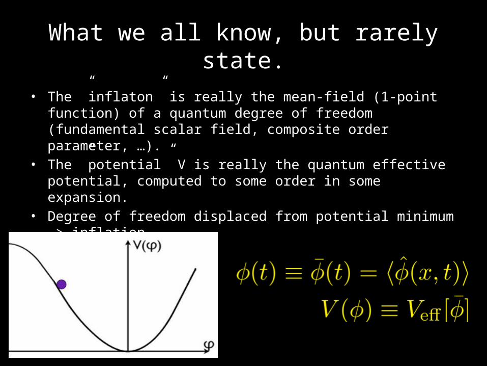
What we all know, but rarely state.• The ”inflaton” is really the mean-field (1-point function) of a quantum
degree of freedom (fundamental scalar field, composite order parameter, …).
• The ”potential” V is really the quantum effective potential, computed to some order in some expansion.
• Degree of freedom displaced from potential minimum -> inflation.
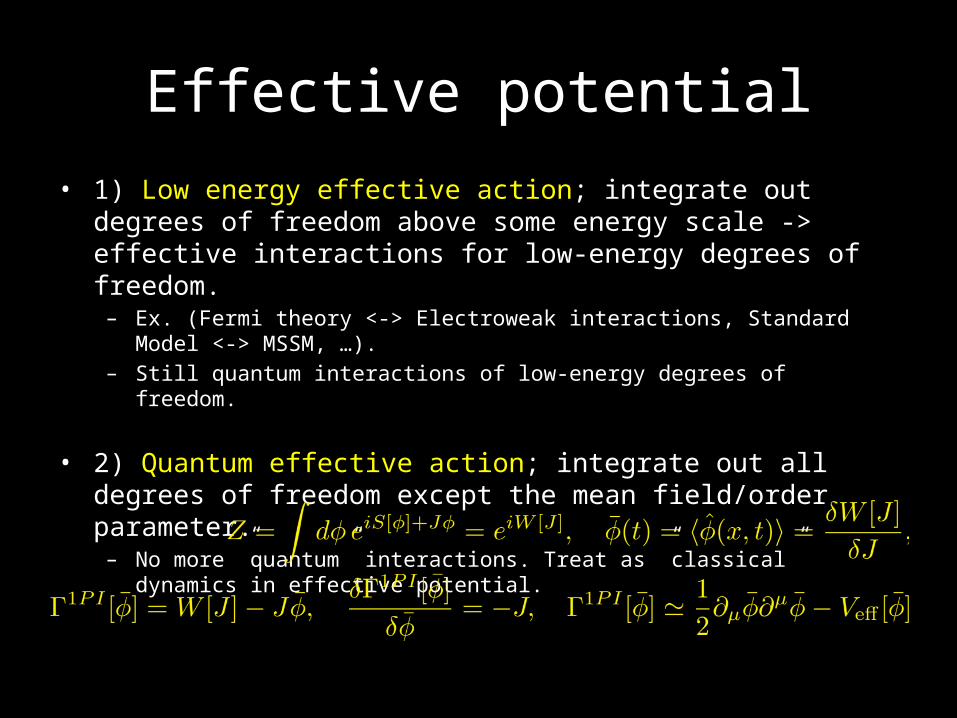
Effective potential• 1) Low energy effective action; integrate out degrees of freedom above
some energy scale -> effective interactions for low-energy degrees of freedom.– Ex. (Fermi theory <-> Electroweak interactions, Standard Model <-> MSSM, …).– Still quantum interactions of low-energy degrees of freedom.
• 2) Quantum effective action; integrate out all degrees of freedom except the mean field/order parameter.– No more ”quantum” interactions. Treat as ”classical” dynamics in effective potential.
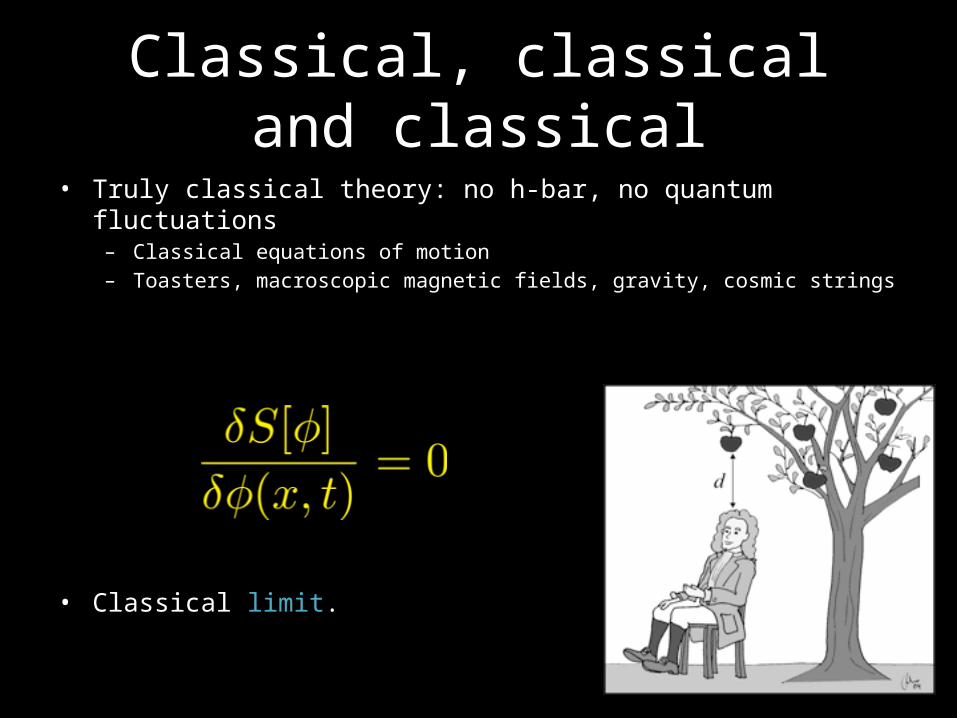
Classical, classical and classical• Truly classical theory: no h-bar, no quantum fluctuations
– Classical equations of motion– Toasters, macroscopic magnetic fields, gravity, cosmic strings
• Classical limit.
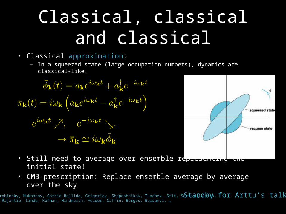
Classical, classical and classical• Classical approximation:
– In a squeezed state (large occupation numbers), dynamics are classical-like.
• Still need to average over ensemble representing the initial state!• CMB-prescription: Replace ensemble average by average over the sky.
Starobinsky, Mukhanov, Garcia-Bellido, Grigoriev, Shaposhnikov, Tkachev, Smit, Serreau, Aarts,AT, Rajantie, Linde, Kofman, Hindmarsh, Felder, Saffin, Berges, Borsanyi, …
Standby for Arttu’s talk!
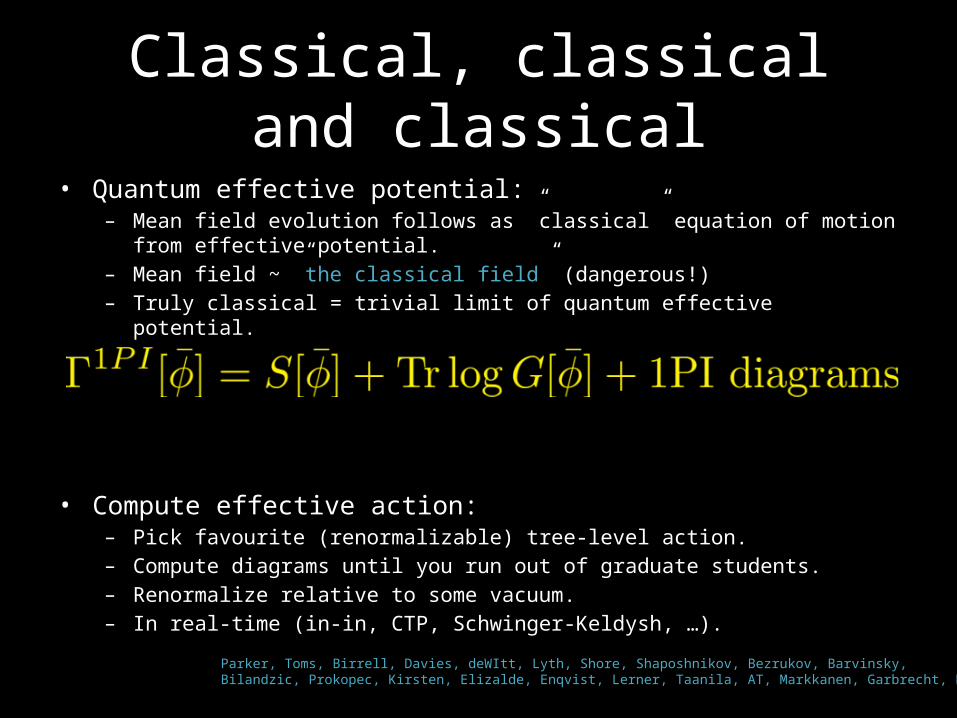
Classical, classical and classical• Quantum effective potential:
– Mean field evolution follows as ”classical” equation of motion from effective potential.– Mean field ~ ”the classical field” (dangerous!) – Truly classical = trivial limit of quantum effective potential.
• Compute effective action:– Pick favourite (renormalizable) tree-level action.– Compute diagrams until you run out of graduate students.– Renormalize relative to some vacuum.– In real-time (in-in, CTP, Schwinger-Keldysh, …).
Parker, Toms, Birrell, Davies, deWItt, Lyth, Shore, Shaposhnikov, Bezrukov, Barvinsky, Bilandzic, Prokopec, Kirsten, Elizalde, Enqvist, Lerner, Taanila, AT, Markkanen, Garbrecht, Postma…
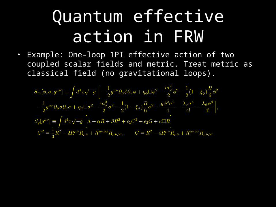
Quantum effective action in FRW• Example: One-loop 1PI effective action of two coupled scalar fields and
metric. Treat metric as classical field (no gravitational loops).
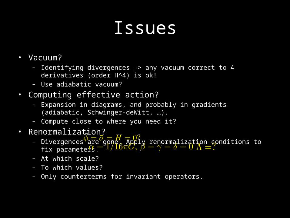
Issues• Vacuum?
– Identifying divergences -> any vacuum correct to 4 derivatives (order H^4) is ok!– Use adiabatic vacuum?
• Computing effective action?– Expansion in diagrams, and probably in gradients (adiabatic, Schwinger-deWitt, …).– Compute close to where you need it?
• Renormalization?– Divergences are gone. Apply renormalization conditions to fix parameters.– At which scale?– To which values?– Only counterterms for invariant operators.

Quantum effective action in FRW• Most general case:
Markkanen, AT: 2012
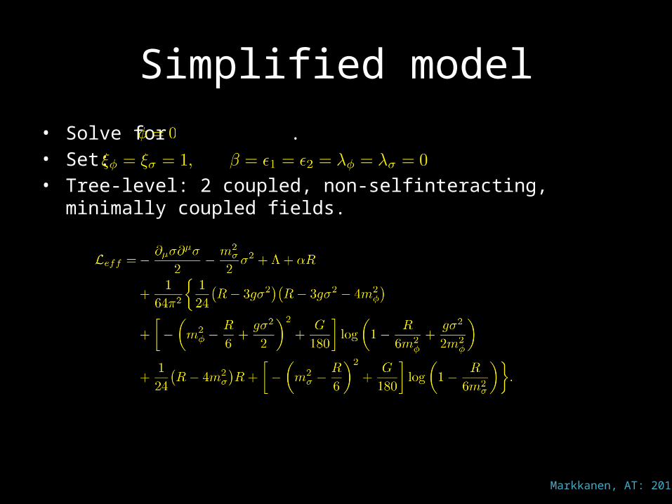
Simplified model• Solve for .• Set:• Tree-level: 2 coupled, non-selfinteracting, minimally coupled fields.
Markkanen, AT: 2012

Scalar field equation of motion• Given background (dS, mat. dom., rad. dom., …):
Markkanen, AT: 2012

Quantum corrected Friedmann eqs.
• Self-consistently solving for the scale factor:
Markkanen, AT: 2012

More issues• Infrared problems for massless fields?
– Because we use ”perturbative” propagators, with mean-field insertions.– Interacting theory -> dynamical mass.
• End of inflation?– Nonperturbative behaviour (reheating, preheating, defects…).– Thermalization, imaginary self-energies.
• Need self-consistent, dynamical propagator equation -> 2PI effective action. Calzetta, Hu, Cornwall, Jackiw, Tomboulis, …
• Serreau 2011: 2PI-resummation to LO -> always non-zero mass in dS. (also Boyanovsky, deVega, Holman, Sloth, Riotto, Parentani, Garbrecht, Prokopec…)
• LO is still Gaussian! NLO AT 2008
• Need a space lattice and a finite number of modes; all eventually redshift into the IR. Problem. AT 2008
• How to renormalize consistently?
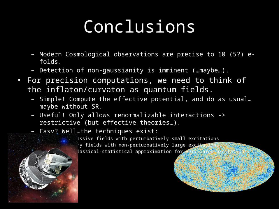
Conclusions– Modern Cosmological observations are precise to 10 (5?) e-folds.– Detection of non-gaussianity is imminent (…maybe…).
• For precision computations, we need to think of the inflaton/curvaton as quantum fields.– Simple! Compute the effective potential, and do as usual…maybe without SR.– Useful! Only allows renormalizable interactions -> restrictive (but effective theories…).– Easy? Well…the techniques exist:
• 1PI for massive fields with perturbatively small excitations• 2PI for any fields with non-perturbatively large excitations.• -> also classical-statistical approximation for very large excitations.