Quantum Field Theory - University of California, Davishiggs.physics.ucdavis.edu/QFT-I.pdf · Class...

Class Notes for Quantum Field Theory: Section IIntroduction to 2nd Quantization, Lagrangian and Equations of Motion, Conservation Laws,

the Klein Gordon field, the Dirac field, Spin-Statistics connection, Feynman Propagators,

Electromagnetic fields

Notes based on Mandl & Shaw, “Quantum FieldTheory”

Best text for later use: Peskin and Schroeder,“Quantum Field Theory”

Jack GunionU.C. Davis

230A, U.C. Davis, Fall Quarter

Outline and Course Goals

1. Become familiar with fields — both classical and quantized.

By “field” we refer to some quantity defined as a function of (~x, t) overall of space-time. An example you are familiar with would be the vectorpotential field A(~x, t) of electromagnetic theory.

2. Learn why we wish to quantize a field and what it means to quantize afield.

3. Learn about the relation between field quantization and particles (somethingthat applies when fields are defined on the space-time continuum) and howthis is a natural extension of the relationship between quantization of ionson a lattice and phonons.

4. Understand the connection: symmetries of the Lagrangian ⇔ conservedquantities.

J. Gunion 230A, U.C. Davis, Fall Quarter 1

5. Learn why every particle must have an antiparticle in a quantized relativistictheory (and the CPT theorem).

6. Understand why a local, Lorentz invariant, causal, 2nd quantized relativisticfield theory must have the observed connection between spin and statistics.

Field Theory

1. Learn about free-particle propagators, especially the difference betweenFeynman, retarded and advanced propagators.

2. Learn about the association between fields and interactions, e.g. E&M field⇒ E&M force.

Also, the association of particles with fields: ⇒ new force requires a newparticle.

3. Develop calculation techniques, i.e Feynman Rules for transition amplitudesand cross sections:

• Perturbation theory.


• Wick’s Theorem.• Time ordered products.

• A simple example of a Feynman diagram is that for e−e− → e−e− viasingle photon exchange. The photon gives rise to the E&M force betweenthe two charged electrons (photons couple to charge).

The photon in this diagram is “virtual” since it has q2 < 0 rather thanq2 = 0. Computing this diagram gives an interaction between the twoelectrons that varies as 1/q2.

This is only the simplest of many very complicated diagrams that should allbe summed together at the amplitude level to obtain the full interaction.Because the charge describing the photon-electron coupling is small, thesimple diagram is a pretty good approximation, but all the other diagramshave some influence.

In particular, the “higher-order” diagrams cause the strength of the inter-electron force to vary with q2 as e2(q2)/q2 where e2(q2) increases as |q2|increases in magnitude.

That is, we can codify the behavior of the diagram sum in terms of a“moving coupling constant” — the momentum dependence of the strength


of the inter-electron force is summarized by an effective coupling strength(effective charge) that varies with momentum.

• For each type of force and matter particle, we will write down a Lagrangiandescribing the interaction of the force particle with the matter particle.

As new forces/particles are discovered, we add new pieces to our Lagrangianand try to organize the Lagrangian so that all the symmetries ... aretransparently displayed.

Ultimate Goal

Write down a single fundamental Lagrangian that describes all the fundamentalparticles and interactions (after “2nd quantization”) that are now relevant orthat were relevant in the past.

• We currently imagine that it was at the time of the big-bang that thelargest number of fundamental particles and forces were “active” and insome kind of short-lived “equilibrium”. Since then, many of the particleshave decayed or annihilated and many of the forces have become irrelevant,leaving us with those observed in every day life and those we can probeusing the accelerators that we have built for this purpose.


• If there is (or was) a “God”, a possible view of his/her role was to choosethis ultimate Lagrangian.

• We currently believe that there might be other causally disconnecteduniverses whose evolution was controlled by a different Lagrangian (orpossibly a version of the same Lagrangian with different “charges” andother parameters).

Theorists even discuss the “anthropic principle” according to which theLagrangian that we “see” is the only one that our form of life could see, butthat there are other forms of life in other universes that “see” a completelydifferent Lagrangian.


System of units and Conventions

Units

• It will be convenient to use a system of units in which h = c = 1.

• In this system of units:

L = T = E−1 = M−1.

e.g. m = mc2 = mch

e.g. me = 9.109× 10−28 g =0.511 MeV (where MeV=106 eV).

• Some convenient conversion factors are:

– (1 GeV)−1 = 0.197× 10−13 cm = 0.197 fermi, where 1 GeV ≡ 109 eV.– (1 GeV)−2 = 0.389 × 10−27 cm2 = 0.389 mb, where mb is short for

milli-barn.


• In Electrodynamics: use so-called Heavyside-Lorentz conventions in whichthe factors of 4π appear in Coulomb’s Law and the fine structure constantrather than in Maxwell’s equations.

i.e. the Coulomb potential for a point charge Q is

Φ =Q

4πr(1)

and the fine structure constant is

α =e2

4π=

e2

4πhc'

1

137(2)

where the latter value actually only applies in the long-wavelength (low-momentum-transfer) limit.

Metric and Lorentz Notation Conventions


• We raise and lower indices and construct Lorentz 4-invariants using

gµν = gµν =

1 0 0 00 −1 0 00 0 −1 00 0 0 −1

(3)

Note that the consistency requirement of gµν = gµαgνβgαβ is satisfied andthat gµν = δµν .

• xµ = (x0, ~x) (careful if you have used Chau’s notes that used to have thisfor xµ contrary to usual definition).

Vectors with raised indices are called “contravariant” and those with loweredindices are “covariant”. xµ = gµνx

ν = (x0,−~x).

• p · x = gµνpµxν = p0x0 − ~p · ~x

• p2 = E2 − |~p|2 = m2

• ∂µ = ∂∂xµ

=(∂∂x0, ~∇

)J. Gunion 230A, U.C. Davis, Fall Quarter 8

• ε0123 = +1, ε0123 = −1, ε1230 = −1, . . ..

• For old “1st quantization”,

E = i ∂∂x0, ~p = −i~∇ which is summarized in the form pµ = i∂µ, where

the raised index accounts for the − sign in ~p = −i~∇.

• Using the notationxµ→ x′µ = Λµνx

ν (4)

for a Lorentz transformation, x′µx′µ = xµxµ requires

ΛλµΛλν = δµν (5)

• If φ(x) is a scalar function, then so is δφ = ∂φ∂xµ

δxµ.

Hence, ∂φ∂xµ≡ ∂µφ ≡ φ, µ is a covariant four-vector.

This is because, a scalar function is such that it is invariant under theLorentz transform, just like the general dot product, ab = aµbµ, so thatsince δxµ is a contravariant vector like aµ, then the object multiplying itto create a scalar function must be a covariant vector.


General Description of what we will be doing andmotivations

Our goal will be to develop Feynman Rules for the calculation of fundamentalprocesses involving elementary particles. A prototype theory for which we wishto develop Feynman rules is QED.

In using Feynman rules for QED, we take a fundamental process involvingphotons and electrons and draw diagrams that can contribute to the processin question. We associate rules for writing down a mathematical expressionfor the Quantum Mechanical amplitude associated with each diagram.

As usual in QM, we sum the amplitudes for all the diagrams and onlytake the square of the net amplitude (which means that different diagramsinterfere with one another).

An example, after extending QED to include muons as well as electrons,would be e+e−→ µ+µ−.


The relevant diagram is

Figure 1: The one Feynman diagram contributing to e+e−→ µ+µ−.

• The presence of spins and different momenta for the particles must all betaken into account in some way.

• The photon connecting the e+e− to the µ+µ− cannot be a real photonsince it must have (p+ k)2 > 0; in fact (p+ k)2 could be very large at ahigh energy collider.

This kind of photon is called “off-shell” or “virtual”.


In quantum mechanics, it is ok for a particle to be off its mass-shell so longas it doesn’t hang around too long (uncertainty principle).

Particles ⇔ Fields

• The association between particles and fields has a long history beginningwith the association of photons with the electromagnetic field.

• In the diagram we just drew, it is the virtual photon that is responsible forthe interaction between the e+e− and the µ+µ− and the virtual photon isa quantum of the electromagnetic field.

• The electrons and muons, and their anti-particles, will turn out to be thequanta of the electron and muon fields.

• Only by using this kind of description in terms of the quanta of the fieldscan we account for processes where particles can be created or annihilated(as in our Feynman diagram).

Relativistic quantum mechanics does not do the job — the Dirac wavefunction for the electron, for example, only describes what a single electron


does in interaction with a potential. Creation or annihilation of that electronis not possible.

Problems for relativistic QM

Some you have hopefully already encountered.

• negative energy states

• Klein Paradox

• probability not easily defined

• probability can “disappear”

Such failures and the need for a field viewpoint could have been anticipated.

• E = mc2 clearly allows for pair creation processes.

Even when energy is inadequate for real pair creation, pair states can appearin 2nd order perturbation theory so long as ∆E∆t <∼ h. (again “virtual”processes)


• Causality is violated.

To see this, let us write transition amplitude for particle propagation from~x0 at t = 0 to ~x at time t. We employ the unitary time translation operatorwhich is given in terms of the Hamiltonian for the particle:

U(t) = 〈~x|e−iHt|~x0〉= 〈~x|e−it

√~P 2op+m2

|~x0〉=

∫d3~p〈~x|e−it

√~P 2op+m2

|~p〉〈~p|~x0〉

=1

(2π)3

∫d3~p e−it

√~p2+m2

ei~p·(~x−~x0) , (6)

Note how we inserted a complete set of plane-wave states I =∫d3~p |~p〉〈~p|

in the momentum basis and used 〈~x|~p〉 = 1

(2π)3/2e−i~p·~x.

Now take ~x0 = ~0 and consider |~x| t (i.e. well outside the light cone),go to one dimension for simplicity, and use stationary phase techniquesfor the exponent ipx − it

√p2 +m2 (with stationary point in p at p =


imx/√x2 − t2) to get

U(t) ∼ exp

−it√− x2m2

x2 − t2+m2 + i

(ixm√x2 − t2

)x

= exp

−it√−t2m2

x2 − t2−

x2m√x2 − t2

= exp

[−m

√x2 − t2

](7)

which is exponentially small, but non-zero, implying that causality is violated.

• Quantum field theory solves this problem by virtue of the fact that there areboth particles and antiparticles propagating across the space-like interval,and their amplitudes cancel one another, thereby preserving causality.

For processes that do not violate causality (i.e. involve a time-likeseparation), this cancellation does not occur (although both particle andanti-particle propagation is occurring).


The Electromagnetic Field – no sources, i.e.“free” field

We will first 2nd quantize this field, since it is the one with which you aremost familiar. We will be glossing over various subtleties in order to developsome intuition.

First let us summarize classical electromagnetic theory. Presumably you allare familiar with:

• Maxwell’s equations

• the choice of a gauge such as the Coulomb (radiation) gauge ~∇ · ~A = 0,

which for a plane wave state ~A(x, t) = ~A0ei(~k·~x−ωt) becomes ~k · ~A = 0.

In this gauge, the equation of motion for ~A becomes 2 ~A = 0 (2 =1c2∂2

∂t2− ~∇2) and

~B = ~∇× ~A, ~E = −1

c

∂ ~A

∂t(8)

for which the Hamiltonian or energy is given by

Hrad =1

2

∫(~E2 + ~B2)d3~x (9)


• We will want to formulate things in Fourier space. In order to keep thingsmost comprehensible, we will go to a finite volume in space, rather thanthe continuum.

We will use periodic boundary conditions in each direction of length L.

Ultimately, the volume V must cancel out of all calculations.

For periodic b.c., the momenta ~k in the box are multiples of 2π/L ineach direction, ~k = 2π

L(n1, n2, n3), ni = 0,±1, . . ., so that in the infinite

volume limit ∑states

=∑

n1n2n3

=L3

(2π)3

∑~k

→V

(2π)3

∫d3~k . (10)

• In our finite volume, we use periodic boundary conditions in the form~A(0, y, z, t) = ~A(L, y, z, t), . . ..

In this case the functions 1√V~εr(~k)ei

~k·~x, r = 1, 2 form a complete set of

transverse orthonormal vector fields.

Here,~εr(~k) · ~εs(~k) = δrs, ~εr(~k) · ~k = 0, r, s = 1, 2 (11)


where the latter equation is required by the radiation gauge ~k · ~A = 0.

The above setup corresponds to a linear polarization basis with polarizationsorthogonal to ~k. We could also employ circular polarizations, but that wouldbe less convenient for the moment, since it is easiest to keep everythingexplicitly real.

• This allows us to expand ~A(~x, t) as a Fourier series:

~A(~x, t) =∑~k

∑r

(hc2

2V ω~k

)1/2

~εr(~k)[ar(~k, t)e

i~k·~x + ar(~k, t)∗e−i

~k·~x](12)

where ω~k = c|~k|. Note that ω~k has dimensions of T−1. The normalizationfactor is chosen quite purposefully as we shall later discuss. The constructionis such that ~A is explicitly real.

• From 2 ~A = 0, we find

∂2

∂t2ar(~k, t) = −ω2

kar(~k, t) . (13)

This is the equation of motion for a harmonic oscillator for each of the


infinitely large number of (r,~k) choices.

The solution is: ar(~k, t) = ar(~k) exp(−iω~kt).

• If we work out Hrad we find

Hrad =∑~k

∑r

hω~ka∗r(~k)ar(~k) , (14)

where h appeared because of the normalization factor appearing in themode expansion of the A field. Note that Hrad is time-independent asexpected for the total electromagnetic energy inside the box (in the absenceof interactions).

• Net result: a perfectly fine reformulation of the classical electromagneticfield. ar(~k) represents a set of numbers and nothing more.

2nd Quantization

• We will quantize the electromagnetic field by hypothesizing that each ofthese infinite number of harmonic oscillator equations should be quantizedin exactly the way we quantize a single harmonic oscillator system, and seewhat happens.


• The way it is actually done, and we will eventually do it this way, is to:

1. treat the fields themselves (at each ~x, t location) as coordinates;2. use the Lagrangian/Hamiltonian of the field theory to determine the

momentum conjugate to the fields when treated as coordinates;3. introduce the analogue of the usual QM commutation relation between

“coordinates” and “momenta”; this is where that√h and other factors

introduced in the normalization of the ~A expansion given in Eq. (12)comes into play. There is an h that we require for the commutator ofthe “coordinate” ~A field with its conjugate “momentum” (∝ ∂

∂t~A).

4. and then reformulate that QM CR in terms of operators in the Fouriertransform space.The above operators are precisely the ar(~k) in the case of the E&Mfield, and so the ar(~k) and a∗r(

~k) objects are no longer simple numbersbut rather operators that work exactly like the a and a† operators of theharmonic oscillator. It is just that there is one such operator for everyr,~k choice.

Harmonic Oscillator Reminder


• Hosc = p2

2m+ 1

2mω2q2 with [q, p] = ih is reinterpreted by writing

a, a† =1

√2hmω

(mωq ± ip), ⇒ [a, a†] = 1 (15)

and simple computation gives Hosc = hω(a†a+ 12).

• One defines a ground state |0〉 with energy 12hω and excited states given

by

|n〉 =(a†)n√n!|0〉 , En = hω(n+

1

2) . (16)

• Further, we go from one occupation number to another via the raising andlowering operators, e.g.

a|n〉 = n1/2|n− 1〉 , a†|n〉 = (n+ 1)1/2|n+ 1〉 . (17)

• By direct computation, for an operator such as a that is time-independent inthe Schroedinger picture, its equation of motion in the Heisenberg picture


(see Appendix to Chapter 1 of Mandl-Shaw for review) is

ihda(t)

dt= [a(t),Hosc] = hωa(t), ⇒ a(t) = ae−iωt . (18)

Back to 2nd quantization of the E&M field

By analogy, we promote ar(~k) and a∗r(~k) to operators ar(~k) and a†r(

~k)obeying the commutation relations

[ar(~k), a†s(~k′)] = δrsδ~k~k′

[ar(~k), as(~k′)] = [a†r(

~k), a†s(~k′)] = 0 , (19)

and write the quantized Hamiltonian operating in the space of states definedbelow as

Hop =∑~k

∑r

hω~k

(a†r(~k)ar(~k) +

1

2

). (20)

Note that the commutation relations assume that each “mode” (~k, r) iscompletely independent of every other mode; i.e. all these pseudo-harmonicoscillator systems are independent of one another.


Note: We can now crudely understand a bit better about the√h in the

normalization factor of the ~A expansion. Roughly, the commutator betweenthe “coordinate” ~A and its conjugate “momentum” takes the form

[Ai(~x, t),∂

∂tAj(~x′, t)] = ihδ3(~x− ~x′)δij , (21)

implying that the√h is needed when we have harmonic oscillator type

normalization for the a and a† commutators, as given above in Eq. (19).

Continuing on, clearly the states

|nr(~k)〉 =[a†r(

~k)]nr(~k)√

nr(~k)!|0〉 (22)

obey

Nr(~k)|nr(~k)〉 = nr(~k)|nr(~k)〉 (23)

where Nr(~k) = a†r(~k)ar(~k). The eigenfunctions of the radiation Hamiltonian


take the form (the |0〉 really only appears once far to the right)

∏~ki

∏ri

|nri(~ki)〉 = |n1(~k1)〉|n2(~k1)〉|n1(~k2)〉|n2(~k2)〉 . . . (24)

and have energy (computed as Hop

∏~ki

∏ri|nri(~ki)〉 ≡ E

∏~ki

∏ri|nri(~ki)〉)

E =∑~k

∑r

hω~k

(nr(~k) +

1

2

). (25)

Raising and lowering works as before: e.g.

ar(~k)| . . . , nr(~k), . . .〉 = [nr(~k)]1/2| . . . , nr(~k)− 1, . . .〉 . (26)

Correspondingly, the eigenvalue of the energy operator, Hop, is reduced by

hω~k = hc|~k|.If we write for the momentum operator the analogue of what we wrote

for the energy operator, Hop, something that we will justify later (it simply


follows from the E&M flux vector ~S), we have

~Pop =∑~k

∑r

h~k

(Nr(~k) +

1

2

)=∑~k

∑r

h~kNr(~k) (27)

and then ar(~k) also reduces the momentum eigenvalue of the state by h~k.We could also get an expression for the angular momentum (using the circularpolarization basis) and by computation show that a single photon state wasone with a single unit of spin.

General Process

• Write down the classical expression for energy, momentum, angular momentum.

• Rewrite this expression by substituting in the “Fourier” expansion of the Afield (but treating a’s and a†’s as operators) and performing the

∫d3~x to

get an operator form of the classical expression.

• Compute what happens when the operator form of the quantity acts upona photon state to see what interpretation is appropriate.

The results we have obtained lead to ....


Interpretation

• ar(~k) is an annihilation operator that removes one photon in the mode(~k, r) of energy hω~k and momentum h~k from the system state.

Thus, our little game gives a result in which the a and a† operators “look,feel, taste, ...” like they annihilate and create a single photon. If furtherinvestigation reveals no conflict with this interpretation, then probably ourguess of how to formulate multi-photon states is correct.

• Our states can have an arbitrary number of photons. In fact, we canhave any number of photons of the same (~k, r) value ⇒ Bose statistics isimplicit.

⇒ something in all this will have to change when we go to fermions.

• You might worry that the ground state (with no photons) has infinite energygiven by

1

2

∑~k

∑r

, (28)

i.e. by the sum of all the “zero-point” energies of the infinite number ofharmonic oscillators.


However, this energy is unobservable in the sense that all we can detectare excitations relative to the ground state.

• Fortunately, the ground state does have zero momentum. Non-zeromomentum would be observable in a very real sense.

• We have not yet checked causality, and we will delay this for a while.

How should we check causality in the context of the operator field ~A(x, t)?We should require

[ ~A(~x, t), ~A(~x′, t′)] = 0 (29)

whenever (t − t′)2 − (~x − ~x′)2 < 0, i.e. when the two operator fields arelocated at a space-like separation they should commute.

By simply carrying out the computation of the commutator using thealgebraic expressions in hand and the commutators for the a’s and a†’s, wefind that this is true.

• However, if we do the same thing for a spin-1/2 Dirac field ψ(~x, t), weencounter a problem.

First, we note that the analogues of the εr(~k)ei~k·~x−iω~kt “plane waves”

are the Dirac spinor forms, us(~k)ei~k·~x−iE~kt, and similarly for the complex


conjugate. (Note that the algebraic form of us(~k) is completely fixed by therequirement that ψ(~x, t) obey the Dirac equation.) The result is that ψ(~x, t)takes the form

ψ(~x, t) =∑~k

∑s

(1

2V E~k

)1/2 [bs(~k)us(~k)e

i~k·~x−iE~kt + d†s(~k)vs(~k)e

−i~k·~x+iE~kt]. (30)

Employing this form, and assuming commutation relations like those forthe E&M a for the b and d operators we don’t get zero when computing[ψ(~x, t), ψ(~x′, t′)] for space-like separations.

We must switch everything from commutation to anticommutation and get0 anticommutator for space-like separation of two Dirac fields.

Is this acceptable? We will see that it is since the Dirac fields themselvesare not observable. The observable operators [e.g. bilinear formslike ψ†(~x, t)ψ(~x, t)] constructed from them will commute for space-likeseparation.

However, because we have fundamental anticommutation relations amongthe creation and annihilation operators, we will have Fermi-Dirac statistics.

• A bit of notation.

It is often convenient to divide the operator field ~A into its positive and


negative frequency components which correspond to the part with theannihilation operator and the part with the creation operator, respectively.

~A(~x, t) = ~A+(~x, t) + ~A−(~x, t) (31)

with

~A+(~x, t) =∑~k

∑r

(hc2

2V ω~k

)1/2

~εr(~k)ar(~k)ei(~k·~x−ω~kt)

~A−(~x, t) =∑~k

∑r

(hc2

2V ω~k

)1/2

~εr(~k)a†r(~k)e−i(

~k·~x−ω~kt)

(32)

Note: e−iωt when operated on by Eop = ih ∂∂t

gives E = +hω.

Summary of differences between 2nd and 1st quantization

2nd quantization refers to the quantization of fields, in which the fieldsthemselves become operators. The coordinates (~x, t) remain simple numbers.


1st quantization refers to non-relativistic or relativistic quantum mechanicsin which we made the ~x coordinate into an operator and obtained a waveequation for a non-operator wave function.

The 2nd-quantized theory, of course, gives the same results as the 1stquantized approach when energies and such are small enough that only 1particle needs to be considered, with creation and annihilation processes beingnegligible.

One final note

By direct calculation

〈state with definite number of photons|~E|same state〉 = 0 (33)

since the ~E field, like the ~A field from which it is computed, either annihilatesor creates an extra photon and then the resulting state does not overlap withthe starting state.

To get a non-zero expectation value for ~E requires that the state inquestion be a superposition of states with different numbers of photons.(Kind of like a wave-packet state in QM can only have a non-zero expectationvalue for both ~x and ~p if it is a superposition of many plane waves.)


Thus, the usual classical ~E fields seen in undergraduate laboratoryexperiments result from a coherent superposition of states with different,but large numbers (in order to have small fluctuation), of photons.

Homework: Do problem 1.2 of Mandl-Shaw.


Appendix: Derivation of e.o.m. for ~A in CoulombGauge

• Maxwell’s equations:

~∇ · ~E = 0 ~∇ · ~B = 0

~∇× ~E = −∂ ~B

∂t~∇× ~B =

1

c2

∂ ~E

∂t(34)

• Move to vector potential.

1. Write~B = ~∇× ~A (35)

then ~∇ · ~B = 0 is automatic.2. Write

~E = −∂ ~A

∂t(36)


then ~∇ · ~E = 0 provided that we are in Coulomb gauge of ~∇ · ~A = 0.

3. ~∇ × ~E = ~∇ × −∂ ~A∂t

= −∂ ~∇× ~A∂t

= −∂ ~B∂t

where we employed Eq. (36)and then Eq. (35). This result implies that the 3rd Maxwell equation isautomatically satisfied.

4. So, it is only the final Maxwell equation that will give a non-trivial e.o.m.for the ~A field. The left hand side of this last ME is:

~∇× ~B = ~∇× (~∇× ~A) = −~∇ · ~∇ ~A+ ~∇(~∇ · ~A) = −~∇ · ~∇ ~A (37)

where we used the Coulomb gauge condition ~∇ · ~A = 0 in the last step.Using Eq. (36), the right hand side is

1

c2

∂

∂t

(−∂ ~A

∂t

)= −

1

c2

∂2 ~A

∂t2(38)

Setting these equal and moving all to one side gives the equation of motion

2 ~A = 0, where 2 =1

c2

∂2

∂t2−∇2 (39)


The Lagrangian Approach

Some intuition from solid state

You could look at Itzykson and Zuber, p. 108 and following for somedetails on this.

• Imagine for the moment that you have a discretized glob of jelly or a solidstate lattice. Each particle in the jelly or ion on the lattice will have its owncoordinate and its own momentum, and, in addition, these particles or ionswill interact with one another in some fashion.

• How would you quantize this system?

You would introduce a qi and pi, i = 1, N (N = very large) for eachparticle, and some potential

∑ij V (xi, xj) and require

[qi, pj] = ihδij. (40)

Here, i and j denote the location of the ions within the lattice, while qi isa displacement coordinate of the ion relative to its central location, and piis the conjugate momentum for this displacement coordinate.


• If you carried this through, then you would find it easiest to deduce theexcitations of this system by defining creation and annihilation operatorsfor (in the lattice example) phonon excitations on the lattice.

You would have a “vacuum” state |0〉 in which all the ions simply had their“zero-point” energy (like a single harmonic oscillator) and then there wouldbe creation operators a†~k that would excite the lattice as a whole to contain

a phonon described by momentum ~k: |~k〉 = a†~k|0〉.

This state would be a state describing a coherent “wave-like” motion ofthe lattice as a whole. The precise energy of the phonon state would bedetermined by such things as the restoring force keeping each ion at itslattice site location and on the potential describing interactions betweendifferent ions on the lattice.

• Now imagine going to the continuum limit of the ion lattice, which would besort of like a jelly. At every (~x, t) location there would be a particle, whosecoordinate location we could denote by φ(~x, t). This latter coordinatelocation can be thought of as the coordinate describing the displacement ofthe ion relative to its central location (~x, t). It is this latter “displacement”coordinate that is the one that should be quantized (just like the simpleharmonic oscillator coordinate is really a displacement coordinate).


We would then want to quantize in a continuum sort of way by definingthe momentum π(~x, t) of this particle (actually π should be a momentumdensity) and require

[φ(~x, t), π(~x′, t)] = iδ3(~x− ~x′) (41)

(I am going to start setting h = 1.)

Note that the δ function makes sense in that if we integrate over a smallvolume in ~x′ and think of φ(~x) as the coordinate of another small volume,and think of each little volume as being a pseudo particle (pp), then theabove would be equivalent to

[coordinate of pp centered at ~x, conj. mom of pp centered at ~x′] = iδ~x~x′ .(42)

If there was more than one degree of freedom at each (~x, t) (such as spindegrees of freedom or the like), we would attach some appropriate index toφ and π and require

[φα(~x, t), πβ(~x′, t)] = iδαβδ3(~x− ~x′) (43)


Field Theory

• In field theory, the coordinates are no longer the coordinates of some ionor jelly component, but rather coordinates in an abstract sense, i.e. really“fields” that appear in a Lagrangian density.

But, we will quantize in exactly the same way as sketched above.

This approach generalizes the classical mechanics of a system of particles,and its quantization, to a continuous system, i.e. to fields ala the treatmentin Goldstein’s Classical Mechanics.

• One introduces a Lagrangian (density) from which the field equations followvia Hamilton’s principle.

• One introduces momenta (density) operators conjugate to the fields andimposes canonical commutation relations between the fields and theseconjugate momenta.

• Everything follows from the Lagrangian density, L. In particular, allconservation laws follow from symmetries of L.


• This approach will give exactly the results we have just described in theE&M field case.

• We will use manifestly relativistic covariant notation.

• We will restrict to theories which can be derived by means of a variationalprinciple from the action

S(Ω) =

∫Ω

d4xL(φr, φr,α) , (44)

where r is some index (like components of ~A) often related to spin andφr,α is the derivative of the field φr as defined by our Lorentz/Metricconventions given earlier.

Note: A Lagrangian which only depends on the fields and their derivativesis not the most general choice, but all cases of interest in this course fallinto this category.

• The fields φr may be real or complex.

In the case that they are complex, the real and imaginary components (orequivalently φ and φ∗) are to be treated as independent objects.


• Postulate that the equations of motion (eom’s) follow from variationalprinciples as follows. Let

φr(x)→ φr(x) + δφr(x) (45)

with δφ vanishing on the surface Γ(Ω) bounding the region Ω.

• Require δS(Ω) = 0 under this variation.

• This leads to (dropping r index for the moment)

δS(Ω) =

∫d4x

[∂L∂φδφ+

∂L∂φ,α

δφ,α

]=

∫d4x

[∂L∂φ−

∂

∂xα

(∂L∂φ,α

)]δφ+

∫d4x

∂

∂xα

(∂L∂φ,α

δφ

)(46)

where the last line follows from partial integration and δφ,α = ∂∂xα

δφ.

• The last term in the last line is zero after using Gauss’s theorem in 4d toconvert the volume integration to a surface integration and using the factthat δφ = 0 on the surface.


• Then, setting δS = 0 and using the fact the δφ at each point within thevolume is independent of other points leads to

∂L∂φ−

∂

∂xα

(∂L∂φ,α

)= 0 (47)

• In order to get the conjugate momenta right, we temporarily discretizespace and time by dividing space up into small cells of equal volume δ~xi,labeled by index i = 1, 2, . . ..

We approximate the values of the fields within each cell by the value at thecenter of the cell.

Think qi(t) ≡ φ(i, t) ≡ φ(~xi, t).

• Write the Lagrangian of the system of cells as

L(t) =∑i

δ~xiLi(φ(i, t), φ(i, t), φ(i′, t)) (48)

where i′ denotes the label of neighboring cells.


• The conjugate momenta to the qi are

pi(t) =∂L

∂qi≡

∂L

∂φ(i, t)≡ π(i, t)δ~xi . (49)

• The Hamiltonian of the discrete system is then given by

H =∑i

piqi − L =∑i

δ~xi

[π(i, t)φ(i, t)− Li

]. (50)

• In the continuum limit (using notation x = (~x, t)), we define π(x) = ∂L∂φ,

and L(t)→∫d3~xL(φ, φ,α) and H(x) = π(x)φ(x)− L(φ, φ,α).

• Since L does not depend explicitly on time, H will be constant in time (aswe shall later prove).

The path integral motivation

• Treating a field as a coordinate probably seems quite adhoc to you.However, the path integral approach provides a very obvious motivation.


• I hope you are all at least vaguely familiar with the fact that normal quantummechanics is equivalent to a path integral formulation in which one writesdown an action (based on a Lagrangian) involving the coordinates andmomenta of the particles involved, and then integrates eiS over all possible“paths” in the coordinate and momentum configuration space:∫

[Dq(t)][Dp(t)]eiS(q,p) . (51)

• The classical path is that for which the action is at an extremum, δS = 0,but in QM one allows for all possible paths with coherent (amplitude level)weighting determined by eiS.

• One can show that this formulation of QM is completely equivalent to thestandard [q, p] = i formulation. This is equivalence is simply a mathematicalidentity.

• So, if we now go to field theory, where “God” gives you a Lagrangian interms of some fields, the simple analogy would be to quantize the theory bygoing to the path integral of eiS, where S is computed from L as describedabove.


• The path integral would now be an integral over all possible values of thefield and its conjugate momentum which are now continuous functions ofthe parameters ~x, t: ∫

[Dφ(~x, t)][Dπ(~x, t)]eiS(φ,π) . (52)

• The same mathematical equivalence would then apply. This path integralapproach to treating this field L quantum mechanically can be shown tobe equivalent to our field quantization conditions where the field at a givenspace time location is treated as a coordinate with non-zero commutatorwith its conjugate momentum

The Klein-Gordon example

• Real scalar field φ(x).

• To derive the Klein-Gordon equation that you may have seen from relativisticquantum mechanics you proceed just as you did for non-relativistic QM:


1. Write down the relationship between energy and momentum, in therelativistic case:

E2 − ~p2 − µ2 = 0 . (53)

Here µ is a constant with mass = (length)−1 dimension that weidentify with the particle’s mass.

2. Replace E → i ∂∂t

and ~p → −i~∇ (we are using h = c = 1 notation)and operate the resulting differential equation on the one-particle wavefunction, which we call φ. The result is:

(−∂2

∂t2+ ~∇2 − µ2)φ(~x, t) = −(2 + µ2)φ(~x, t) = 0 . (54)

This is the KG equation.

• The Lagrangian that gives this equation of motion is

L =1

2(φ,αφ

α, − µ

2φ2) . (55)

Proof: We first must compute, using dummy indices β, γ and metric tensor


for the first term in L,

∂L∂φ,α

=∂

∂φ,α

(1

2gβγφ,βφ,γ

)=

1

2gβγ [δβαφ,γ + φ,βδγα]

=1

2

[gαγφ,γ + gβαφ,β

]= φα, .

Thus, we have

∂L∂φ

= −µ2φ ,

∂L∂φ,α

= φα, =∂φ

∂xα,

∂

∂xα

(∂L∂φ,α

)=

∂

∂xα

(∂φ

∂xα

)= 2φ

⇒∂L∂φ−

∂

∂xα

(∂L∂φ,α

)= 0→ −(2 + µ2)φ = 0 .


• The EOM, (2 + µ2)φ(x) = 0, being the Klein-Gordon equation ⇒ thequantized degrees of freedom that will be associated with it will turn outto be spinless neutral bosons.

Note that the L form is quite abstract until we make this connection.

• Note: The Lagrangian density is not completely determined by the equations of motion. The standard Euler-Lagrange form of

the eom will be unchanged if we add to the Lagrangian density a total four derivative ∆L = ∂βΛβ provided Λβ has the form

Λβ = f(φ)φβ, , so that the β index is supplied by the field derivative, but there are no further field derivatives. In this case, wehave

∂∆L∂φ

= ∂α∂Λα

∂φ= ∂α

(∂f

∂φφα,

)(56)

and

∂

∂xα

(∂∆L∂φ,α

)=

∂

∂xα

(∂β

∂Λβ

∂φ,α

)=

∂

∂xα

(∂βfg

αβ)

=∂

∂xα

(∂αf)

=∂

∂xα

(∂f

∂φφα,

)(57)

and we see that ∂∆L∂φ− ∂∂xα

(∂∆L∂φ,α

)= 0. If we wanted to consider a more complicated form of Λβ such that f = f(φ,A),

with A = φ,γφγ, , we would have to go back and rederive the equations of motion from δS = 0. They would be more

complicated than the usual due to the fact the ∆L depends upon 2nd derivatives of φ (which we did not allow for in our

derivation) in a rather complicated way. The theorem would still apply in that the new equations of motion obtained from δS = 0

allowing for 2nd derivatives in the full L would be left unaltered by the addition of ∆L.

• Conjugate momentum: π(x) = ∂L∂φ(x)

= φ(x) by direct computation.


• The Hamiltonian density computation.

H = πφ− L= π2 −

1

2

[π2(x)− (~∇φ)2 − µ2φ2

]=

1

2

[π2(x) + (~∇φ)2 + µ2φ2

].

(2nd) Quantization

• Impose “usual” canonical commutation relations:

[φ(j, t), p(j′, t)] = [φ(j, t), π(j′, t)δ~xj′] = iδjj′δ~xj , (58)

with other commutators zero.

In the continuum limit, you can think of dividing by δ~xj to obtain

[φ(~x, t), π(~x′, t)] = iδ3(~x− ~x′) (59)


along with other commutators = 0.

Note that the commutation relations are at equal time, as always is thecase for standard quantization.

• In the Klein-Gordon case, the important non-zero commutator reduces to

[φ(~x, t), φ(~x′, t)] = iδ3(~x− ~x′) (60)

Symmetries and Conservation Laws

• Heisenberg eom ⇒ idO(t)dt

= [O(t),H] = 0 if [O,H] = 0.

• [O,H] = 0 generally derives from invariance properties under a group oftransformations.

e.g. translational and rotational invariance lead to conservation of linearand angular momentum, respectively.

Such transformations lead to equivalent descriptions of the system; in theabove case the descriptions are the same in two Lorentz frames related bya translation or a rotation


• Quantum mechanically, two such descriptions must be related by a unitarytransformation U

|Ψ〉 → |Ψ′〉 = U |Ψ〉 , O → O′ = UOU† . (61)

The above relations imply:

1. Operator equations are covariant (i.e. take the same form in terms oforiginal or transformed operators).In particular, this is true of the commutation relations of the fields andof the equations of motion. For example, consider the commutationrelation. Let us compute the commutator in the prime system to seeif we get the same result as in the unprimed system. We have (usingx = (t, ~x), x′ = (t, ~x′))

[φ′(x), π′(x′)] = [φ′(x)π′(x′)− π′(x′)φ′(x)]

= [Uφ(x)U†Uπ(x′)U† − Uπ(x′)U†Uφ(x)U†]

= U [φ(x), π(x′)]U†

= Uiδ3(~x− ~x′)U† = iδ3(~x− ~x′) , (62)

using U†U = 1 (unitarity). Here, it was important to note that U


is some complicated operator that contains creation and annihilationoperators but should (except in special cases, such as rotation andtranslation that also change the coordinates) commute with δ3(~x− ~x′).In the special cases, the coordinate arguments are also shifted to newcoordinate arguments.Another example is that Maxwell’s equations will take the same form intwo different frames.

2. Amplitudes and, hence, observable predictions are invariant under thetransformation. An example here is to consider a typical expectationvalue for which we have:

〈Ψ′|O′|Ψ′〉 = (〈Ψ|U†)(UOU†)(U |Ψ〉) = 〈Ψ|O|Ψ〉 (63)

using the unitarity of U .

• For continuous transformations, we can write

U = eiαTα→0∼ 1 + iαT , with T = T † (64)

(T is called the generator of the transformation U .) for which

O′ = O + δO = (1 + iαT )O(1− iαT ) , ⇒ δO ' iα[T,O] (65)


If the theory is invariant under U , then H will be invariant, i.e. δH = 0.Plugging O = H into the above equation implies [T,H] = 0, i.e. T is aconstant of motion.

• For a field theory derived from a L, conserved quantities can be constructedfrom the invariance of L under symmetry transformations.

The procedure is known under the name “Noether’s Theorem”.

The Noether approach to obtaining conserved quantities

• Will show that an invariance of L under a symmetry transformation willalways lead to an equation of the form

∂fα

∂xα= 0 (66)

where the fα are functions of the field operators and their derivatives.

• Then, as you well know, we can define the spatial integrals

Fα(t) =

∫d3~xfα(~x, t) (67)


and use Eq. (66) to derive

dF 0(t)

dt= −

∫d3~x

3∑j=1

∂

∂xjf j(~x, t) = 0 (68)

where the last equality comes from converting to a surface integral usingGauss’s theorem and from assuming the fields (and hence the f j) vanishsufficiently fast at infinity.

In short, F 0 is a conserved quantity and one can construct the correspondingunitary operator for the transformation by setting T = F 0.

So, now let us prove this theorem.

• Suppose that L is invariant under φ(x)→ φ′(x) = φ(x) + δφ(x).

• However, we may always use the chain rule to compute δL under anytransformation:

δL =∂L∂φδφ+

∂L∂φ,α

δφ,α =∂

∂xα

(∂L∂φ,α

δφ

)(69)


where the last equality follows from the eom for φ:

∂L∂φ−

∂

∂xα

(∂L∂φ,α

)= 0 (70)

given earlier. Since, by assumption for the particular transformation wehave δL = 0, we see that Eq. (69) implies that

fα =∂L∂φ,α

δφ (71)

is a conserved current and the constant of motion is

F 0 =

∫d3~xπ(x)δφ(x) . (72)

• Thus, for a given L, all that remains is to determine the field transformationsfor which δL = 0. For each such transformation, there will be a conservedcurrent and a constant of motion.

The simplest example: complex scalar field


• A particularly important and yet simple example is provided by

L = φ†,αφα, − µ

2φ†φ (73)

where φ is a complex field (vs. the real field case considered earlier). (Therationale for the different normalization compared to the earlier real-fieldcase will eventually be explained.)

• The above L is invariant under

φ′ = eiεφ ' (1 + iε)φ φ† ′ = e−iεφ† ' (1− iε)φ† , (74)

where ε is a real parameter and we are taking ε to be infinitesimal in size.

Thus, we have an invariance with δφ = iεφ and δφ† = −iεφ†.

• The corresponding conserved quantity is

F 0 = iε

∫d3~x

[π(x)φ(x)− π†(x)φ†(x)

](75)

where π(x) = ∂L∂φ(x)

= φ†(x) and π†(x) = ∂L∂φ†(x)

= φ(x).


• If F 0 is conserved then so is

Q = −iq∫d3~x

[π(x)φ(x)− π†(x)φ†(x)

](76)

as obtained using ε = −q. Here, ±q will turn out to be the electric chargesof the particle and antiparticle associated with the field φ.

• We can easily show that Q generates the symmetry transformation bycomputing φ′(x) = eiQφe−iQ which, in the infinitesimal limit (here thelimit of small q), reduces to

δφ = i[Q,φ(x)] = i

[−iq

∫d3~x′[π(x′), φ(x)]φ(x′)

]= q

∫d3~x′[−iδ3(~x− ~x′)]φ(x′)

= −iqφ(x) (77)

which is correct for the ε = −q identification made earlier. In the above, weused the fact that φ only has non-zero commutator with its correspondingπ(x) (remembering that φ and φ† are independent fields in the complexfield case).


• [Q,φ] = −qφ tells us something else as well. Namely, suppose that |Q′〉 isan eigenstate of the operator Q with eigenvalue Q′. Then, we find

Qφ|Q′〉 = [Q,φ]|Q′〉+ φQ|Q′〉 = (Q′ − q)φ|Q′〉 (78)

which in words says that operating with φ on |Q′〉 has reduced the chargeof the state by one unit of q. This is because φ contains an annihilationoperator for the particle with charge q and a creation operator for theantiparticle with charge −q, as we shall later verify when we return to 2ndquantizing the field φ.

• Note: If the field φ is real, it will not be possible to define a charge for thefield.

• The above type of symmetry is called a global (i.e. x-independent) phasesymmetry or a gauge invariance of the first kind.

• Possible ambiguities associated with the ordering of the operators in theexpression for Q will be resolved, once we have carried through the 2ndquantization procedure, by requiring Q|0〉 = 0 for the vacuum state inwhich no particles (associated with the field φ) are present.


Energy, Momentum and Angular Momentum

• Conservation of energy and momentum and of angular momentum followsfrom the invariance of L under translations and rotations.

Since these transformations form a continuous group, we need only considerinfinitesimal transformations.

• However, there is an extra piece in the analysis that did not appear for thephase rotations just considered.

• The transformations are defined by:

x′α ≡ xα + δxα = xα + εαβxβ + δα , (79)

where δα is the infinitesimal displacement and εαβ = −εβα is an infinitesimalantisymmetric tensor (as required to ensure that xαxα is invariant whenδα = 0) specifying an infinitesimal rotation.


• The above transformation will induce (and here we need to bring back thepossible spin indices on the field)

φ′r(x′) = φr(x) +

1

2εαβS

αβrs φs(x) . (80)

• It is important to keep in mind that x′ and x label the same physical point;it is just that this physical point is specified by a different set of coordinatevalues in the two different frames.

• The Sαβrs depend upon the “representation” or nature of the spin carriedby the field. If the field in question is the vector field Aα(x), then the S’swould simply correspond to the usual rules for transformation of a vectorfield. (Do you know for sure what these look like in the infinitesimal limit?)

• Invariance under the transformations above means that L, when expressedin terms of the x′ and φ′(x′) must have the same functional form aswhen expressed in terms of x and φ(x). If this is the case, then thefield equations will be covariant, i.e. they will have the same form whenexpressed in terms of either the original or the transformed coordinates andfields.


An example in the real scalar field case is that

L(φ′(x′), φ′,α(x′)) =1

2

[φ′,α(x′)φ

′ α, (x′)− µ2φ′(x′)φ′(x′)

], (81)

which would obviously lead to the same form for the equations of motionas found in the original frame where

L(φ(x), φ,α(x)) =1

2

[φ,α(x)φ α

, (x)− µ2φ(x)φ(x)]

; (82)

it would just be that everything had a prime in the primed frame case.

• Further, since L should be a scalar, it should have the same value at a givenphysical point, regardless of what frame is used to describe the physicalpoint: i.e.

L(φr(x), φr,α(x)) = L(φ′r(x′), φ′r,α(x′)) . (83)

For the scalar field Lagrangian, this is obviously the case since φ is a scalarfield for which φ′(x′) = φ(x) (the field should take the same value at thesame physical point). Thus, indeed L(φ′(x′), . . .) = L(φ(x), . . .).


Note: We are implicitly employing the passive point of view (i.e. wechange to a different coordinate system and that is all) in this treatment.Other treatments employ an active point of view and the derivations looksomewhat different.

• To return to Noether’s theorem, let us examine the consequences ofEq. (83) obtained by expanding the right-hand side in terms of the unprimedcoordinates and fields by means of using the transformations (79) and (80).

– We again define δφr(x) ≡ φ′r(x)−φr(x) as the variation of φr with theargument unchanged.

– In addition we will need δTφr(x) ≡ φ′r(x′) − φr(x), i.e. the variation

including the change in the argument.– We then have:

δTφr(x) = [φ′r(x′)− φr(x′)] + [φr(x

′)− φr(x)]

= δφr(x′) +

∂φr

∂xβδxβ

' δφr(x) +∂φr

∂xβδxβ (84)

where the last approximation neglects doubly-small terms.


– Similarly, we write

0 = L(φ′r(x′), φ′r,α(x′))− L(φr(x), φr,α(x))

= δL+∂L∂xα

δxα , (85)

where δL = L(φ′(x), . . .) − L(φ(x), . . .), i.e. only x appears when weneglect doubly-small changes.

– For δL we proceed as we did in the phase case and write

δL =∂L∂φr

δφr +∂L∂φr,α

δφr,α

=∂

∂xα

[∂L∂φr,α

δφr

]=

∂

∂xα

[∂L∂φr,α

(δTφr −

∂φr

∂xβδxβ

)]. (86)

where the first equality just follows from the good old eom’s and for the2nd equality we use Eq. (84).

– From this result, it is clear that a suitable choice of the conserved current


is

fα ≡∂L∂φr,α

δTφr − T αβδxβ (87)

with

T αβ ≡∂L∂φr,α

∂φr

∂xβ− Lgαβ , (88)

which is the standard energy-momentum tensor.In more detail, using Eq. (88) in Eq. (87) we have

∂fα

∂xα=

∂

∂xα

[∂L∂φr,α

(δTφr −

∂φr

∂xβδxβ

)]−

∂

∂xα

(−Lgαβδxβ

)= δL+

∂L∂xα

δxα

= 0 (89)

where the last 0 comes from Eq. (85). Note that δxβ is some fixed shiftin x defined by our original symmetry statement, implying that ∂

∂xαdoes

not operate on it.

• Let us now apply this to a translation:

εαβ = 0⇒ δxβ = δβ and φ′r(x′) = φr(x) ,


which in turn⇒ δTφr(x) = 0 , (90)

which in turn implies (see Eq. (87)) that

fα = −T αβδβ . (91)

Since each of the 4 δβ’s are independent of one another, this really impliesthat there are four conserved currents and four conserved charges, thelatter being the spatial integrals of T 00, T 01, T 02, and T 03, i.e. it is usefulto define

P β =

∫d3~xT 0β =

∫d3~x

[πr(x)

∂φr(x)

∂xβ− Lg0β

], , (92)

which is just the (operator corresponding to) the energy-momentum four-vector, with explicit components

P 0 =

∫d3~x [πr(x)φr(x)− L] =

∫d3~xH = H (93)


and

P j =

∫d3~xπr(x)

∂φr(x)

∂xj. (94)

These are the momentum operators expressed in terms of the field operators.This will be confirmed when we express these operators in terms of thenumber representation that follows from the 2nd quantization procedure.

Homework 2: At this point, you are ready to do Problems 2.2, 2.3 and 2.4from Mandl-Shaw.

• Now consider the Noether current for a L symmetric under rotation:

In this case, we have δxβ = εβγxγ and δTφr(x) = 1

2εβγS

βγrs φs(x), where

we have used appropriate indices and dummy summation indices for whatfollows.

Plugging this into Eq. (87), i.e. into

fα ≡∂L∂φr,α

δTφr − T αβδxβ (95)


gives

fα =∂L∂φr,α

1

2εβγS

βγrs φs(x)− T αβεβγxγ

=1

2

[∂L∂φr,α

Sβγrs φs(x)− T αβxγ + T αγxβ]εβγ (96)

where the 2nd equality follows by using the antisymmetry of εβγ.

Now, we note that the εβγ are all independent, which gives us a whole setof six different conserved currents denoted as

Mαβγ ≡∂L∂φr,α

Sβγrs φs(x)− T αβxγ + T αγxβ (97)

yielding 6 conserved quantities for α = 0

Mβγ =

∫d3~xM0βγ

=

∫d3~x

[xβT 0γ − xγT 0β

]+ πr(x)Sβγrs φs(x)

. (98)

So what are all these objects?


– For two spatial indices (i, j = 1, 2, 3), M ij is the angular momentumoperator of the field (M12 being the z-component, etc.).

– For one spatial index i and one 0 index, we get the operator giving riseto boosts in the i direction.

– Within the expression of Eq. (98), the [. . .] stuff is the orbital angularmomentum and the S term contains the portion of the total angularmomentum coming from the intrinsic spin of the field.

Reiteration of Basic Steps and Points

• Nature will give us a certain type of field and a certain Lagrangian densityfor this field.

• We will (2nd) quantize this system by treating the field as if it were aquantum mechanical coordinate, using the Lagrangian density to define themomentum density conjugate to the field (just as we would for a jelly ordense lattice).

• Indeed, everything follows from L.

In particular, any conserved quantity must be associated with an invarianceof L.


If the theory is to be translationally invariant, then L should be invariantunder translations and the corresponding conserved quantity (the momentumoperator) must be that obtained by applying the Noether construction tothe translationally invariant L.

If the theory is to have a conserved electric charge (or similarly forhypercharge and other such things), L must be invariant under a globalphase rotation (or some other abelian phase transformation), and theassociated charge operator must come from the Noether construction usingthe phase transformation.

More complicated groups are also possible, where there is another (non-spin) index attached to the field that transforms in some non-trivial wayunder a group generated, for example, by a Lie algebra.

We will now turn to carrying out this procedure in detail for:

1. the real and complex scalar fields.

2. the Dirac field.

3. the electromagnetic field.

in that order.


The Scalar Field

Basics for a real scalar field

• For one particle wave equation, we began with E2 = µ2 + ~p2, madereplacements ~p → −i~∇, E → i ∂

∂tand obtained the Klein-Gordon

equation:(2 + µ2)φ(x) = 0 . (99)

• We recall that one of the “difficulties” of this equation was the presence ofnegative energy solution.

This difficulty is characteristic of single-particle wave equations. We willsee that such difficulties do not arise in the 2nd quantization (i.e. fieldquantization) approach.

• We saw earlier that the KG equation is the equation of motion coming from

L =1

2(φ,αφ

α, − µ

2φ2) (100)


and that the field (momentum density) conjugate to φ is

π(x) =∂L∂φ

= φ . (101)

We quantize the system by turning φ into a hermitian operator and requiring

[φ(~x, t), φ(~x′, t)] = iδ3(~x−~x′) [φ(~x, t), φ(~x′, t)] = [φ(~x, t), φ(~x′, t)] = 0 .(102)

To implement these quantization conditions we expand φ with operatorcoefficients, just as already done for the ~A field earlier, assuming for themoment periodic conditions in a box:

φ(x) = φ+(x) + φ−(x) (103)

with

φ+

(x) =∑~k

(1

2ω~kV

)1/2

a(~k)e−ik·x

, φ−

(x) =∑~k

(1

2ω~kV

)1/2

a†(~k)e

+ik·x(104)

Here, k0 = ω~k =

√µ2 + ~k2: i.e. k = (k0, ~k) is the on-mass-shell

(on-shell, for short) four momentum of a relativistic particle of mass µ.


You should be asking yourself why the appropriate expansion functions aree±ik·x, where k · x = ω~kt− ~k · ~x. The answer is that we should expand interms of the “plane wave” solutions of the equation of motion obeyed byφ, i.e. the solutions of the Klein-Gordon equation that is determined by theLangrangian. We can check that these plane waves are indeed solutions:

(2 + µ2)e−ik·x =

(∂2

∂t2− ~∇2 + µ2

)e−iω~kt+i

~k·~x

=(−ω2

~k+ ~k2 + µ2

)e−iω~kt+i

~k·~x

= 0 provided ω2~k

= ~k2 + µ2

i.e. provided ω~k is given by the appropriate relativistic form for a particleof mass µ.

You should also ask yourself why it is that we have chosen φ− to be theHermitian conjugate of φ+. This is because we have chosen to discuss thecase of a real (before quantization) scalar field, the quantized version ofwhich should be a Hermitian field.

• So, now that we have an appropriate expansion of the field φ in termsof operator coefficients, we must determine the commutation relations of


the a and a† such that the 2nd quantization condition of Eq. (102) aresatisfied.

The quantization conditions of Eq. (102) are achieved by requiring

[a(~k), a†(~k′)] = δ~k~k′ , [a(~k), a(~k′)] = [a†(~k), a†(~k′)] = 0. (105)

We should prove this as an if and only if statement. I will prove it in theeasy direction below. You will prove it in the harder direction as homework.

Homework 3: MS problem 3.1 is to show that if [φ(~x, t), φ(~y, t)] =iδ3(~x− ~y) (and others are 0) then the above commutators are as stated.

Here we show the reverse, which is actually easier. We check that if thea, a† commutators are as stated, then [φ(~x, t), φ(~y, t)] = iδ3(~x− ~y).

Proof:

[φ(~x, t), φ(~y, t)] =[∑~k

(1

2V ω~k

)1/2

(a(~k)e−ik·x + a†(~k)e+ik·x),

∑~p

(1

2V ω~p

)1/2

(−iω~pa(~p)e−ip·y + iω~pa†(~p)e+ip·y)

]J. Gunion 230A, U.C. Davis, Fall Quarter 71

=∑~k,~p

(1

2V ω~k

)1/2(1

2V ω~p

)1/2 [iω~pe

ip·y−ik·x[a(~k), a†(~p)]

−iω~pe−ip·y+ik·x[a†(~k), a(~p)]]

=i

V

∑~p

e−i~p · (~y−~x) →i

(2π)3

∫d3~pe−i~p · (~y−~x) = iδ3(~x− ~y) (106)

where we used x0 = y0 = t for equal time commutators and for the2nd term in the next to last line did a change of summation variablesfrom ~k, ~p → −~k,−~p, and of course used the fact that [a(~k), a†(~p)] =

−[a†(−~k), a(−~p)] = δ~k~p, which also means that we can set ω~p = ω~keverywhere. When this is done in the exponential, the time dependencedisappears, as it must. Of course, it is important to keep in mind thatω~k is an even function of ~k. We have noted that the evaluation of themomentum sum is most easily done by going to the large volume limit inthe standard way and using the usual integral representation of the Diracdelta function.

• A note on normalization conventions


In writing the operator expanion of φ using the 1√2V ω~k

normalization and

in writing the a, a† commutator as [a(~k), a†(~p)] = δ~k~p, we made twoconnected normalization choices. Obviously, we could make a change in theφ expansion normalization convention provided we made a compensatingchange in the [a(~k), a†(~p)] normalization, adjusting one relative to theother so that we maintain [φ(~x, t), φ(~y, t)] = iδ3(~x − ~y), which is ourfundamental physics input assumption.

• In any case, the a, a† commutators are precisely the Harmonic oscillatorcommutators as already discussed for the ~A field, and we know how toproceed. In particular, we establish a occupation number space with numberoperator

N(~k) = a†(~k)a(~k) (107)

with eigenvalues n(~k) = 0, 1, 2, . . ., with a(~k) and a†(~k) being theannihilation and creation operators of particles with four-momentum k.

– We define the vacuum state by a(~k)|0〉 = 0, which also impliesφ+(x)|0〉 = 0.

– We define a single particle state via |~k〉 = a†(~k)|0〉.


– We define two-particle states (correctly normalized) by

|~k,~k′〉 = a†(~k)a†(~k′)|0〉, ~k 6= ~k′

|~k,~k〉 =1√

2[a†(~k)]2|0〉 (108)

It is perhaps useful to perform the manipulations that demonstrate whythere is a 1/

√2 in the last equation. The point is that all states should

have the same normalization. So, let us assume that 〈0|0〉 = 1 forconvenience. Then, we wish to check the normalization of |~k,~k〉:

〈~k,~k|~k,~k〉 =1

2〈0|aaa†a†|0〉

=1

2〈0|a(1 + a†a)a†|0〉

=1

2〈0|aa†|0〉+

1

2〈0|aa†aa†|0〉

=1

2〈0|(1 + a†a)|0〉+

1

2〈0|aa†(1 + a†a)|0〉

=1

2〈0|0〉+

1

2〈0|0〉 = 〈0|0〉


where we stopped writing ~k, used [a, a†] = 1 (for the same value of ~k)repeatedly, and used a|0〉 = 0 several times.

– We clearly have Bose statistics since the order of the a† operators fora multiparticle state does not matter (a† operators commute with oneanother) and since we can put as many particles into the same ~k stateas we like.

• We already know what the Hamiltonian and momentum operators are fromNoether’s theorem applied to the scalar-field L:

H =

∫d3~x

1

2

[φ2 + (~∇φ)2 + µ2φ2

]~P = −

∫d3~x φ~∇φ . (109)

• We now just substitute the expansion form of φ to see what we get. Wefind

H =∑~k

ω~k

[N(~k) +

1

2

], ~P =

∑~k

~kN(~k) . (110)


Prove this as part of homework 3.

These expressions are the “proof” that the a(~k) and a†(~k) operators areindeed the annihilation and creation operators for a relativistic spinlessparticle, in the sense that if it smells like a ... and tastes like a ...., then itis a ....

More explicitly, let us examine the one particle state, |~k〉 = a†(~k)|0〉. Wehave

N(~k′)|~k〉 = a†(~k′)a(~k′)a†(~k)|0〉= a†(~k′)[δ~k′~k + a†(~k)a(~k′)]|0〉= δ~k′~ka

†(~k)|0〉+ 0

= δ~k′~k|~k〉

from which we find that

H|~k〉 =

ω~k +∑~k′

1

2ω~k′

|~k〉 (111)


as compared to

H|0〉 =∑~k′

1

2ω~k′|0〉 (112)

which is to say that the 1-particle state has an energy that is ω~k larger thanthe energy of the vacuum state.

Note that the H operator has only positive energy excitations, relative tothe vacuum state.

Similarly, we have~P |~k〉 = ~k|~k〉 (113)

as compared to~P |0〉 = 0 (114)

which is to say that the 1-particle state has a momentum that is ~k ascompared to the vacuum state having no momentum.

Thus, it really looks like the 1-particle state that we have defined doesindeed have the energy and momentum of a relativistic 1-particle state.Again, it should be emphasized that once we had specified L and the 2ndquantization condition, we had no freedom in how to compute the H and~P operators.


• Well, there is another normalization convention here.

When I wrote the Lagrangian for the real scalar field, I made a certain choiceof the normalization. The Klein Gordon equation would result from theeom no matter what the overall normalization of L is. The normalizationconvention was chosen so that the energy that comes out of Noether’stheorem is the normal energy and not say 917 × E~k or something of thesort.

Of course, we made long ago a historical choice for how to define the unitsof energy and momentum, and that is built into what we have done. Aphrase that is sometimes used is to say that the normalization employedfor L is “canonical normalization”. Whenever we write a Lagrangian, itis important to write it with canonical normalization for each degree offreedom (each particle after 2nd quantization).

Thus, when we come to the charged scalar field (complex scalar field) ina short while, L will be chosen without a factor of 1/2 in front. Thisis because each of the two independent degrees of freedom (particle andantiparticle) should carry canonically normalized energy. The form that willbe chosen (without the 1/2) gives exactly this result.

• We see above that the vacuum |0〉 will have H|0〉 =∑~k′

12ω~k′|0〉, which is


infinite because we are summing an infinite number of zero-point harmonicoscillator energies.

But, this infinity is unmeasurable. We only see excitations relative to it.This is just like a big lattice. The lattice would have an enormous groundstate energy from all the zero-point ion energies, but all we would careabout are the energies of the phonon excitations relative to this big groundstate energy.

• It is convenient to always write things in such a way that this infinity isthrown away. The formal name for doing so is “normal ordering” or alwaysusing “normal products”, denoted by N . By definition, N instructs us toput all the a† operators to the left of the a operators. For example:

N(a(~k1)a(~k2)a†(~k3)) = a†(~k3)a(~k1)a(~k2) (115)

and

N [φ(x)φ(y)] = N [(φ+(x) + φ−(x))(φ+(y) + φ−(y))]= φ+(x)φ+(y) + φ−(x)φ+(y)

+φ−(y)φ+(x) + φ−(x)φ−(y) , (116)


where the order of the factors was changed only in the 3rd term, so thatall φ+ operators (which contain the annihilation operator) are to the rightof all φ− operators.

Note, some minus signs will creep into the definition of N when fermionsare involved.

Sometimes N [. . .] is denoted by : [. . .] :, to avoid confusion with thenumber operator.

• Clearly, the vacuum expectation value of any normal product vanishes.Thus, it is convenient to define all observables as being normal ordered. Inparticular, starting from our original form of H,

N [H] =∑~k

ω~k1

2N [a(~k)a†(~k) + a†(~k)a(~k)] =

∑~k

ω~ka†(~k)a(~k) . (117)

From now on, when we write H, we will be assuming that it is the normal-ordered version of H that is being written. Thus, for example, we will


have

H|~k〉 =

∑~k′

ω~k′N(~k′)

|~k〉 = ω~k|~k〉 . (118)

using the same result, N(~k′)|~k〉 = δ~k′~k|~k〉, as before.

Basics for a complex scalar field

• WriteL =: (φ†,αφ

α, − µ

2φ†φ) : (119)

Treating the field and its adjoint as independent fields, leads to the KGequations

(2 + µ2)φ(x) = 0 , (2 + µ2)φ†(x) = 0 . (120)

• The fields conjugate to φ and φ† are π = φ† and π† = φ.

• The equal-time quantization conditions are then

[φ(~x, t), φ†(~x′, t)] = iδ3(~x− ~x′)[φ(~x, t), φ(~x′, t)] = [φ(~x, t), φ†(~x′, t)] = [φ(~x, t), φ(~x′, t)]


= [φ(~x, t), φ†(~x′, t)] = [φ(~x, t), φ(~x′), t)] = 0 (121)

Note that the first, i.e. the non-zero, commutator is equivalent to theother commutator that must be non-zero, namely

[φ†(~x, t), φ(~x′, t)] = iδ3(~x− ~x′) . (122)

• These commutation relations are solved in the operator basis by:

φ(x) = φ+(x) + φ−(x) =∑~k

(1

2ω~kV

)1/2 [a(~k)e−ik·x + b†(~k)e+ik·x

](123)

with φ†(x) being the hermitian conjugate of the above, provided

[a(~k), a†(~k′)] = [b(~k), b†(~k′)] = δ~k~k′ (124)

with all other commutators being zero.

• Once again, we can interpret (as we shall see), a(~k) and b(~k) as annihilation


operators and a†(~k) and b†(~k) as creation operators, but this time for twodifferent types of particles.

The corresponding vacuum state is defined by

a(~k)|0〉 = b(~k)|0〉 = 0, all ~k . (125)

The number operators for the two different types of particles are

Na(~k) = a†(~k)a(~k) , Nb(~k) = b†(~k)b(~k) . (126)

• To understand how to interpret these two different types of particleoperators we must evaluate the energy and momentum operators forthis system.

One finds that the four-momentum operator takes the form (recall that His now defined as including the normal-ordering prescription)

Pα = (H, ~P ) =∑~k

kα (Na(~k) +Nb(~k)) (127)


where we should keep in mind that k0 = ω~k. This result means that botha† and b† create particles from the vacuum state with the four momentumof a relativistic particle with mass µ.

• So what is it that distinguishes the a from the b particles?

Let us look at charge. We obtained an expression for the charge operatorfrom L from its global phase invariance. Including normal ordering (whichmeans that we throw away an infinite charge for the vacuum state andmeasure charges of other states relative to the vacuum charge) we have:

Q = −iq∫d3~x : [φ†(x)φ(x)− φ(x)φ†(x)] : (128)

which reduces to

Q = q∑~k

[Na(~k)−Nb(~k)] , (129)

demonstrating that the b type particle is the antiparticle of the a typeparticle with exactly the same mass but opposite charge.


The corresponding charge-current density is given by

jα(x) = (ρ(x),~j(x)) = −iq : [∂φ†

∂xαφ−

∂φ

∂xαφ†] : (130)

which obviously (use the fact that φ and φ† both obey the KG equation)satisfies

∂jα(x)

∂xα= 0 . (131)

Notes:

– The energy operator is positive definite, unlike what happens in trying tointerpret the single particle Klein-Gordon plane wave solutions.

– If one describes a charged particle using a relativistic quantized fieldtheory, one inevitably finds that there is an antiparticle with oppositecharge (and other such quantum numbers) but with exactly the samemass.

– If the field is real, the charge operator is zero, but a chargeless particlecan still have an antiparticle.This occurs if there are other charge-like properties of the particle. Anexample is what is called hypercharge. The neutral meson K0 with

hypercharge Y = 1 has an antiparticle K0

with Y = −1.


At this point, problem 3.2 of Mandl-Shaw is assigned, as well as the extraproblem in which you are asked to derive the expression for Q of Eq. (129).

Propagators for the scalar field

• The first example of a propagator is the covariant commutator of two fields:[φ(x), φ(y)], where x and y are two different coordinate locations.

It should be a covariant scalar since the theory is supposed to be covariantand since the fields are scalars. However, the equal time commutatorsmight have broken this in some way, but they do not.

• We first note that

[φ(x), φ(y)] = [φ+(x), φ−(y)] + [φ−(x), φ+(y)] (132)

since the + components commute with one another and the − componentsalso commute with one another.


• For the 1st term we get

[φ+(x), φ−(y)] =1

2V

∑~k~k′

1√ω~kω~k′

[a(~k), a†(~k′)]e−ik·x+ik′·y

V→∞→1

2(2π)3

∫d3~k

ω~ke−ik·(x−y)

≡ i∆+(x− y) , (133)

where we have employed the δ~k~k′ commutator and we must keep inmind that k0 and k′ 0 are the on-shell energies. We have also used1V

∑~k →

1(2π)3

∫d3~k for the continuum limit [see Eq. (10)].

• Similarly, one finds

[φ−(x), φ+(y)] = −[φ+(y), φ−(x)] = −i∆+(y − x) ≡ i∆−(x− y) .(134)

• Altogether, we have

[φ(x), φ(y)] = i∆(x− y) = i∆+(x− y) + i∆−(x− y)


= −i

(2π)3

∫d3~k

ω~ksin[k · (x− y)] , (135)

and, removing the i’s, we have

∆(x) = −1

(2π)3

∫d3~k

ω~ksin k · x . (136)

• Note that (2x + µ2)∆(x− y) = 0 by virtue of the fact that φ(x) satisfiesthis equation. This means that ∆(x−y) is not a propagator. “Propagator”is just another word for Green’s function, and a Green’s function shouldgive a Dirac δ function when acted on by the equation of motion.

• We can also write

∆(x− y) =−i

(2π)3

∫d4kδ(k2 − µ2)ε(k0)e−ik·(x−y) , (137)

where d4k = dk0d3~k now lets k0 run from −∞ to +∞, but then if we


write the δ function in the form

δ(k2 − µ2) =1

2ω~k[δ(k0 + ω~k) + δ(k0 − ω~k)] (138)

we see that it picks out k0 = ±√~k2 + µ2 and these terms get combined

with the correct sign by virtue of the definition

ε(k0) ≡ k0/|k0| =

+1, if k0 > 0−1, if k0 < 0

. (139)

This form makes it clear that ∆(x − y) is an invariant under (proper, i.e.no parity or time reversal) Lorentz transformations since each factor in theintegrand is Lorentz invariant. (Here, ε(k0) is Lorentz invariant since properLorentz transformations do not interchange past and future and k0 onlyappears unsquared as a multiplier of x0 − y0.)

• Returning to the issue of causality, we have

[φ(x), φ(y)] = i∆(x− y) = 0 for (x− y)2 < 0 (140)


by virtue of

1. the fact that

[φ(~x, t), φ(~y, t)] = 0 = i∆(~x− ~y, 0) ; (141)

2. the fact that ∆(x− y) is a Lorentz invariant; and3. the fact that we can go from the equal time frame where we know the

answer from the equal time commutation relation to any other framewith (x− y)2 < 0 via a proper Lorentz transformation.

We can also think about this more directly. As we know,

∆(x) = ∆+(x) + ∆−(x) = ∆+(x)−∆+(−x)

=−i

(2π)3

∫d3~k

2ω~k[e−ik·x − e+ik·x] . (142)

Now, if x2 < 0, we can perform a continuous Lorentz transformation onthe 2nd term taking x → −x. (If x2 > 0, this is not possible as it wouldmove us from inside the forward light cone to inside the backward lightcone.) After this transformation, the two terms cancel.


• The contour integration representation of ∆

We can write (using the complex variable residue theorem)

∆±(x) = −1

(2π)4

∫C±

d4ke−ik·x

k2 − µ2(143)

where the contours are viewed as contours in the k0 complex plane, C+ is asmall circular counter-clockwise contour around the pole of the denominatorat k0 = +ω~k and C− is a small counter-clockwise contour around the poleat k0 = −ω~k.

For example, for ∆−, we write

k2 − µ2 = (k0)2 − ~k2 − µ2 = (k0 − ω~k)(k0 + ω~k)

∼ −2ω~k(k0 − (−ω~k)) , (144)

and via the residue theorem find that


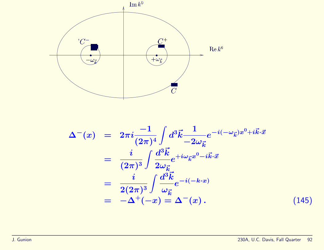
∆−(x) = 2πi−1

(2π)4

∫d3~k

1

−2ω~ke−i(−ω~k)x0+i~k·~x

=i

(2π)3

∫d3~k

2ω~ke+iω~kx

0−i~k·~x

=i

2(2π)3

∫d3~k

ω~ke−i(−k·x)

= −∆+(−x) = ∆−(x) . (145)


∆(x) = ∆+(x) + ∆−(x) is then given by the same integral form for alarge counter-clockwise contour that circles around both poles.

The Feynman propagator

• This will be the propagator that actually enters into our calculations.

However, the simplified treatment of MS, will not allow a formal derivationof this fact.

• To begin, first note that

i∆+(x− y) = 〈0|[φ+(x), φ−(y)]|0〉 = 〈0|φ+(x)φ−(y)|0〉= 〈0|φ(x)φ(y)|0〉 (146)

where the first equality simply follows from the fact that the vacuumexpectation value of a non-operator quantity (a “c-number”) is simplyequal to the c-number. The 2nd equality follows from the fact that〈0|φ−(y)φ+(x)|0〉 = 0 by virtue of the fact that φ+ contains theannihilation operator that annihilates the vacuum. The final equality isdue to the fact that all terms in φ(x)φ(y) other than φ+(x)φ−(y) givezero (because of a|0〉 = 0 and/or 〈0|a† = 0).


Further,

− i∆−(x− y) = i∆+(y − x) = 〈0|φ(y)φ(x)|0〉 . (147)

• We now define the “time-ordered”, or T , product by

Tφ(x)φ(y) =

φ(x)φ(y), if x0 > y0

φ(y)φ(x), if y0 > x0

= θ(x0 − y0)φ(x)φ(y) + θ(y0 − x0)φ(y)φ(x) .(148)

That is, the operators are written in chronological order.

• The Feynman propagator is defined as the vacuum expectation value of thetime-ordered product:

i∆F (x− y) = 〈0|Tφ(x)φ(y)|0〉 . (149)

so that, using the earlier vacuum expectation value results of Eqs. (146)and (147), we have

∆F (x) = θ(x0)∆+(x)− θ(−x0)∆−(x) . (150)


• Referring back to Eq. (149), we can think of ∆F (x− y) as representing ameson created at y and then traveling to x when x0 > y0 and vice versa.

However, one should note that this time ordering picture is frame-dependent. What really enters a calculation in which a virtual mesonis exchanged between two scattering particles is the sum of the two timeorderings as incorporated in ∆F , which is a covariant functional form.

To be more precise, consider the scattering of two nucleons, n1 and n2,via the exchange of a spin-0 “meson” described by our KG field. If wekeep track of time-orderings, there is one diagram in which n1 first emitsthe φ at time t1 which is then later absorbed by n2 at time t2 (t2 > t1case) and there is a 2nd time ordering in which n2 first emits the φ attime t2 and then the φ is later absorbed by n1 at time t1 (t1 > t2 case).The full scattering amplitude must account for both cases, since we shouldintegrate over all possible values of t1 and t2. The Feynman propagatorautomatically accounts for the two possibilities.

• One should not be concerned that ∆F (x− y) 6= 0 if (x− y)2 < 0 (space-like separation). A physical meson is not actually traveling faster than thespeed of light between x and y; it is a virtual meson. As a result, a realprocess at x (e.g. a particle emitting an on-shell meson which then travels


to y and is reabsorbed there) is not influencing a real process at y.

Do new problem assigned at this point involving a “different” propagator.

• Let us check explicitly that ∆F is a Green’s function. We do this by firstcomputing

∂2

∂x02i∆F (x− y)

=∂2

∂x02〈0|Tφ(x)φ(y)|0〉

= 〈0|∂2

∂x02

[θ(x

0 − y0)φ(x)φ(y) + θ(y

0 − x0)φ(y)φ(x)

]|0〉

= 〈0|[∂

∂x0

([∂

∂x0θ(x

0 − y0)

]φ(x)φ(y) + θ(x

0 − y0)∂

∂x0φ(x)φ(y)

)

+∂

∂x0

([∂

∂x0θ(y

0 − x0)

]φ(y)φ(x) + θ(y

0 − x0)φ(y)

∂

∂x0φ(x)

)]|0〉

= 〈0|[∂

∂x0

(δ(x

0 − y0)φ(x)φ(y) + θ(x

0 − y0)∂

∂x0φ(x)φ(y)

)

+∂

∂x0

(−δ(x

0 − y0)φ(y)φ(x) + θ(y

0 − x0)φ(y)

∂

∂x0φ(x)

)]|0〉


= 〈0|[(

∂

∂x0δ(x

0 − y0)

)φ(x)φ(y) + 2δ(x

0 − y0)∂

∂x0φ(x)φ(y) + θ(x

0 − y0)∂2

∂x02φ(x)φ(y)

+

(−∂

∂x0δ(x

0 − y0)

)φ(y)φ(x)− 2δ(x

0 − y0)φ(y)

∂

∂x0φ(x) + θ(y

0 − x0)φ(y)

∂2

∂x02φ(x)

]|0〉

= 〈0|[

+δ(x0 − y0

)∂

∂x0φ(x)φ(y) + θ(x

0 − y0)∂2

∂x02φ(x)φ(y)

−δ(x0 − y0

)φ(y)∂

∂x0φ(x) + θ(y

0 − x0)φ(y)

∂2

∂x02φ(x)

]|0〉

= 〈0|[

+δ(x0 − y0

)[π(x), φ(y)] + θ(x0 − y0

)∂2

∂x02φ(x)φ(y) + θ(y

0 − x0)φ(y)

∂2

∂x02φ(x)

]|0〉

= 〈0|[−δ(x

0 − y0)iδ

3(~x− ~y) + θ(x

0 − y0)∂2

∂x02φ(x)φ(y) + θ(y

0 − x0)φ(y)

∂2

∂x02φ(x)

]|0〉

= 〈0|[−iδ4

(x− y) + θ(x0 − y0

)∂2

∂x02φ(x)φ(y) + θ(y

0 − x0)φ(y)

∂2

∂x02φ(x)

]|0〉 (151)

where we used some partial integrations to remove derivatives on the δfunctions, and used the equal time commutator for [φ(y), π(x)]. The finalstep is to bring in the −~∇2

x + µ2 part of the 2x operator, which doesnot operate on the θ functions (since they only contain the time variables)which gives


(2x + µ2)i∆F (x− y)

= 〈0|[−iδ4

(x− y) + θ(x0 − y0

)(2x + µ2)φ(x)φ(y) + θ(y

0 − x0)φ(y)(2x + µ

2)φ(x)

]|0〉

= −iδ4(x− y) , (152)

where the last step just uses the fact that (2x + µ2)φ(x) = 0.

• A reminder about Green’s functions:

In general, the Green’s function for a differential equation, defined byoperator Ox (here we use notation appropriate for a one-dimensionalproblem with coordinate x) is defined by the fact that it allows a solutionto the equation Oxf(x) = j(x), where j(x) is some source term. Asyou know, f(x) will consist of a sum of homogeneous solutions and aninhomogenous component. The Green’s function solution to this equationis to write

f(x) =

∫dyG(x− y)j(y) , (153)

which will satisfy Oxf(x) = j(x) if OxG(x − y) = δ(x − y). Anotherphraseology is that if j(y) is a localized impulse, j(y) = δ(y − y0),then f(x) = G(x − y0) is the response to that localized impulse. In


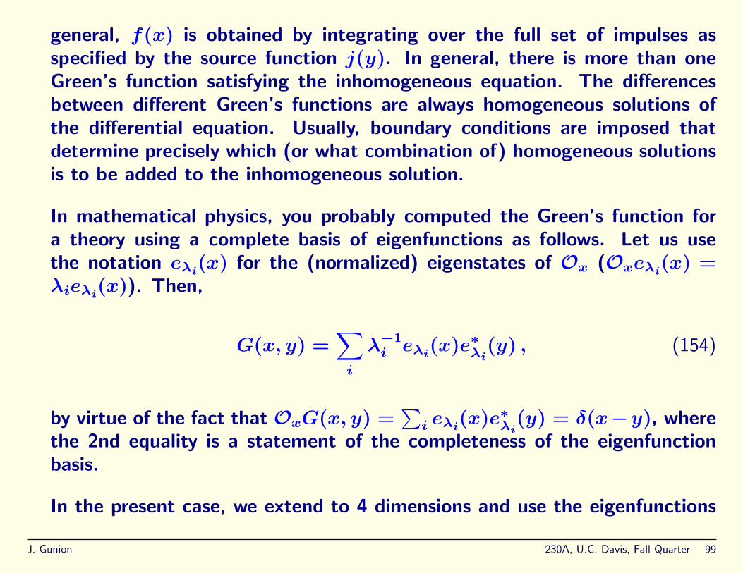
general, f(x) is obtained by integrating over the full set of impulses asspecified by the source function j(y). In general, there is more than oneGreen’s function satisfying the inhomogeneous equation. The differencesbetween different Green’s functions are always homogeneous solutions ofthe differential equation. Usually, boundary conditions are imposed thatdetermine precisely which (or what combination of) homogeneous solutionsis to be added to the inhomogeneous solution.

In mathematical physics, you probably computed the Green’s function fora theory using a complete basis of eigenfunctions as follows. Let us usethe notation eλi(x) for the (normalized) eigenstates of Ox (Oxeλi(x) =λieλi(x)). Then,

G(x, y) =∑i

λ−1i eλi(x)e∗λi(y) , (154)

by virtue of the fact that OxG(x, y) =∑i eλi(x)e∗λi(y) = δ(x−y), where

the 2nd equality is a statement of the completeness of the eigenfunctionbasis.

In the present case, we extend to 4 dimensions and use the eigenfunctions


ek(x) = 1(2π)2e

−ik·x which have

(2x + µ2)ek(x) = (−k2 + µ2)ek(x) ≡ λkek(x) (155)

(note that we don’t require on-shell k2 = µ2 — we want all possibleeigenvalues and not just the homogenous modes) and are normalizedaccording to

1

(2π)4

∫d4x eip·xe−ik·x = δ4(k − p) . (156)

Thus,

G(x− y) =

∫d4k

1

(2π)2eik·x

1

−k2 + µ2

1

(2π)2e−ik·y

=1

(2π)4

∫d4k

eik·(x−y)

−k2 + µ2. (157)

Here, we allow an extra minus sign, which is sort of a convention as tohow to define a Green’s function. Different Green’s functions are definedby different ways of evading the denominator singularity (which is obviouslyclosely related to what homogenous solutions, i.e. those with k2 = µ2 areincluded).


• The contour representation of ∆F

We will show that

∆F (x) =1

(2π)4

∫CF

d4ke−ik·x

k2 − µ2(158)

where the contour CF runs along the real k0 axis, passing above the poleat k0 = +ω~k and below the pole at k0 = −ω~k.

Note: if this expression is correct, then (2x+µ2)∆F (x−y) = −δ4(x−y)(using integral rep. of δ4 function) in agreement with above result.


• First, we note that for x0 > 0, we can close the contour in the lower 1/2plane without picking up any contribution from the big half circle in thelower 1/2 plane (since e−ik

0x0 ∝ e−i(iImk0x0) ∼ e(Imk0)x0

is damped whenImk0 < 0 and x0 > 0. The resulting contour is equivalent to C+, exceptfor the clockwise direction, and we see that we get ∆F (x) = ∆+(x) whenx0 > 0, where we recall the result of Eq. (143):

∆±(x) = −1

(2π)4

∫C±

d4ke−ik·x

k2 − µ2(159)

• If x0 < 0, we close in the upper 1/2 plane. The contour is equivalent toC− (including contour direction), and we get ∆F (x) = −∆−(x).

• These results are in agreement with the earlier result

∆F (x) = θ(x0)∆+(x)− θ(−x0)∆−(x) . (160)

• It is very useful to give another form for the expression of Eq. (158) usinga different contour. The idea is that we can move the k0 contour to lie


exactly along the real axis provided we displace the poles by an infinitesimalamount in the correct direction. Defining η to be > 0 and very small,

– the k0 = −ω~k pole should be displaced by +iη into the upper 1/2 plane;– the k0 = +ω~k pole should be displaced by −iη into the lower 1/2 plane.

This is equivalent to replacing the denominator k2 − µ2 = (k0)2 − ω2~k

by

[k0 − (ω~k − iη)][k0 + (ω~k − iη)]

= [k0]2 −(ω~k − iη

)2∼ [k0]2 − ω2

~k+ iε

= [k0]2 − [~k2 + µ2] + iε= k2 − µ2 + iε (161)

where we defined ε = 2ηω~k which is again an infinitesimally small > 0quantity.

• Exactly equivalent results are obtained for the complex scalar field:

〈0|Tφ(x)φ†(y)|0〉 = i∆F (x− y) (162)


where ∆F is exactly the same function with the same contour representationsas in the real scalar field case.


The Dirac Field

Anticommutator basics

• For Dirac fields (obeying the Dirac equation) We will convert fromcommutation conditions to anticommutation conditions for quantization(as we shall detail in a moment).

This also leads to a perfectly satisfactory number representation, butone implicitly based on Fermi statistics for the particles being created orannihilated.

This choice is required by causality (along with other basic requirements)in the field theory context.

• The bosonic quantization in terms of the ar, a†r operators (r = 1, 2, . . .denoting momentum states) required the commutation relations

[ar, a†s] = δrs , [ar, as] = [a†r, a

†s] = 0 (163)


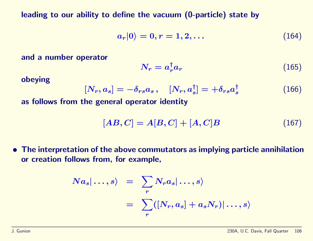
leading to our ability to define the vacuum (0-particle) state by

ar|0〉 = 0, r = 1, 2, . . . (164)

and a number operatorNr = a†rar (165)

obeying[Nr, as] = −δrsas , [Nr, a

†s] = +δrsa

†s (166)

as follows from the general operator identity

[AB,C] = A[B,C] + [A,C]B (167)

• The interpretation of the above commutators as implying particle annihilationor creation follows from, for example,

Nas| . . . , s〉 =∑r

Nras| . . . , s〉

=∑r

([Nr, as] + asNr)| . . . , s〉


=∑r

(−δrsas + asNr)| . . . , s〉

= as(−1 +N)| . . . , s〉= (n− 1)as| . . . , s〉 (168)

where we assumed N | . . . , s〉 = n| . . . , s〉. In fact, it is precisely the sstate that has been removed from | . . . , s〉. This can be checked once aLagrangian has been specified and we know how to specify the physicalproperties (e.g. E, ~P , charge, ...) of a given state s.

• However, there is an alternative way to get a number operator obeying thecreation and annihilation commutators of Eq. (166), based on using theanticommutator

[A,B]+ ≡ A,B ≡ AB +BA , (169)

for which we have

[AB,C] = A[B,C]+ − [A,C]+B . (170)


We need only require anticommutator quantization conditions,

[ar, a†s]+ = δrs , [ar, as]+ = [a†r, a

†s]+ = 0 (171)

to obtain exactly the same results as in Eq. (166) for Nr by using Eq. (170).

For example,

[Nr, as] = [a†rar, as] = a†r[ar, as]+ − [a†r, as]+ar= 0− δrsar = −δrsas . (172)

This leads to the interpretation of ar, a†r and Nr = a†rar as annihilation,creation and number operators operating on states based on the vacuumstate defined by ar|0〉 = 0.

• For this setup, it is clear that we have Fermi-Dirac statistics.

For example, if we try to create 2 particles in the same state via a†ra†r|0〉,

we can rewrite this as 12[a†r, a

†r]+|0〉 which is zero because of the last

anticommutator quantization condition of Eq. (171).


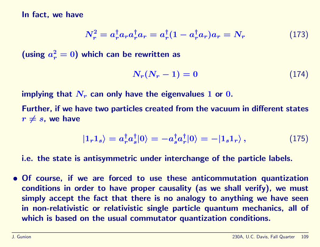
In fact, we have

N2r = a†rara

†rar = a†r(1− a

†rar)ar = Nr (173)

(using a2r = 0) which can be rewritten as

Nr(Nr − 1) = 0 (174)

implying that Nr can only have the eigenvalues 1 or 0.

Further, if we have two particles created from the vacuum in different statesr 6= s, we have

|1r1s〉 = a†ra†s|0〉 = −a†sa

†r|0〉 = −|1s1r〉 , (175)

i.e. the state is antisymmetric under interchange of the particle labels.

• Of course, if we are forced to use these anticommutation quantizationconditions in order to have proper causality (as we shall verify), we mustsimply accept the fact that there is no analogy to anything we have seenin non-relativistic or relativistic single particle quantum mechanics, all ofwhich is based on the usual commutator quantization conditions.


The Dirac Equation

• Recall that KG equation began with the relativistic energy momentumrelation

E2 = c2~p2 + µ2c4 (176)

followed by substitutions E → ih ∂∂t

, ~p → −ih~∇ , yielding the waveequation (h = c = 1)

(2 + µ2)φ(x) = 0 (177)

with solutions φ = ei(~k·~x−ω~kt) with ω~k = ±(~k2 + µ2)

12. The problem was

that E = ih ∂∂t

gave positive energy for one choice but negative energy forthe other choice.

• Dirac wanted to start with an equation that was linear in E by roughlytaking the square root of Eq. (176). Beginning with

i∂

∂tψ(~x, t) = Hψ(~x, t) (178)


his first thought was to write this in terms of E and ~k as

E = (~k2 +m2)12 (179)

followed by E → i ∂∂t

, ~p → −i~∇ . (We use m instead of µ for the Diracequation.)

But, this obviously leads to an equation where time and space are treatedasymmetrically implying that the equation is not relativistically covariant.

• At the very least, one needs an equation that is linear in ~k as well as in E.A general form is

H = ~α · ~k + βm (180)

leading to

(E − ~α · ~k − βm)ψ = 0 , (181)

and, thence, the wave equation

(i∂

∂t+ i~α · ~∇− βm)ψ = 0 . (182)


• Now, what about the ~α and β objects. They cannot have explicitdependence on ~x or t, or derivatives with respect to the same, as suchdependence would lead to space time dependent energy and therefore giverise to forces, whereas the equation we seek is one for a free particle.

• So, the only choices for ~α and β are numbers or matrices. We learn moreby requiring that any solution ψ of Eq. (182) also be a solution of the KGequation (but not vice versa). This is a reasonable requirement since, in theabsence of external fields, the wave packet solutions of Eq. (182) shouldhave the classical relation between energy, momentum and mass. So, letus multiply Eq. (181) on the left by (E + ~α · ~k + βm) to obtain

[E2 − (α2

xk2x + α2

yk2y + α2

zk2z) + (αxαy + αyαx)kxky+

(αzαy + αyαz)kzky + (αxαz + αzαx)kxkz −m2β2

−m (αxβ + βαx)kx + (αyβ + βαy)ky + (αzβ + βαz)kz]ψ

= 0 . (183)

To agree with the relativistic energy momentum relationships we requirethe following identities


α2x = α2

y = α2z = β2 = 1

αxαy + αyαx = αyαz + αzαy = αzαx + αxαz = 0αxβ + βαx = αyβ + βαy = αzβ + βαz = 0 (184)

i.e. the four quantities anticommute in pairs and their squares are unity.The smallest representation of this algebra is for αi and β to be 4 × 4matrices (see Schiff QM Sec. 52 for more detail on this).

The choice of Dirac was

β =

(1 00 −1

), ~α =

(0 ~σ~σ 0

)(185)

where the σi are the 2 × 2 Pauli matrices and the 1’s are 2 × 2 unitmatrices:

σx =

(0 11 0

)σy =

(0 −ii 0

)σz =

(1 00 −1

)(186)

which we know anticommute and have unit square (implying the same forthe αi). That β and the αi anticommute is apparent from the explicitexpressions above.


• So, now let us return to the basic Dirac equation, which you have seen canbe written in the form

ih∂ψ(x)

∂t= [c~α · (−ih~∇) + βmc2]ψ(x) , (187)

where I have temporarily reintroduced h and c. In this equation ~α and β

are 4 × 4 matrices, and ψ is a 4-component object: ψ =

ψ1

ψ2

ψ3

ψ4

, where

the individual components are often denoted ψα, α = 1, 2, 3, 4, where α isreferred to as the Dirac index of the spinor.

Very often, as above, we will write equations in such a way that this Diracindex and the matrix etc. multiplications are implicit rather than explicit.Thus, for example, in the above equation there is an implicit Dirac index,call it ρ, and the last term could be written more explicitly as βρλψλ(x).

The Dirac equation can be written (after multiplying the equation by β andusing β2 = 14×4, the 4 × 4 identity matrix) in a more covariant looking


form (setting h = c = 1),

iγµ∂ψ(x)

∂xµ−m14×4ψ(x) = 0 (188)

by definingγ0 ≡ β , γi = βαi , i = 1, 2, 3 , (189)

where these “Dirac matrices” γµ obey the anticommutation relations

[γµ, γν]+ = 2gµν14×4 , (190)

and the hermiticity conditions

γ0 † = γ0 , γj † = −γj j = 1, 2, 3 , (191)

so that (using the anticommutation relation also)

γµ† = γ0γµγ0 . (192)

Usually, one does not explicitly write the 14×4 matrix. It is understood tobe present in the matrix equations we will be writing.


Note: The above hermiticity properties guarantee hermiticity of theHamiltonian and momentum operators constructed below.

• There is more than one specific numerical representation of these γ matrices.

The so-called Dirac representation is that you may have already seen, and ismost useful for discussing the low-energy, non-relativistic limit of the Diracequation.

A better representation for high-energy applications is the so-called Weylor chiral representation that is discussed in detail in Peskin and Schroeder.

We will avoid as long as possible writing down any specific representation.All representations of the matrices are related by unitary transformations.

• In a more general context, one could arrive at this collection of γµ matricesby showing that they form the simplest general representation of the Lorentzgroup structure beyond the usual vector representation.

Later, we will give enough information about this approach in order thatwe can specify what the form of the rotation and Lorentz transformationgenerators is.


• We will define an adjoint field

ψ(x) = ψ†(x)γ0 , (193)

which, by starting with the Dirac equation for ψ(x), is easily shown tosatisfy

i∂ψ(x)

∂xµγµ +mψ(x) = 0 . (194)

Note that any given component of the adjoint field ψα is independent of theψα component of the non-adjoint field since ψα is a complex quantity and hasan independent real and imaginary part. This is the analogue of the statementthat φ and φ† are independent objects when dealing with a complex scalarfield.

The Dirac Lagrangian

• In order to proceed with the 2nd quantization game, we must first find aLagrangian that yields the Dirac equation as its equation of motion.


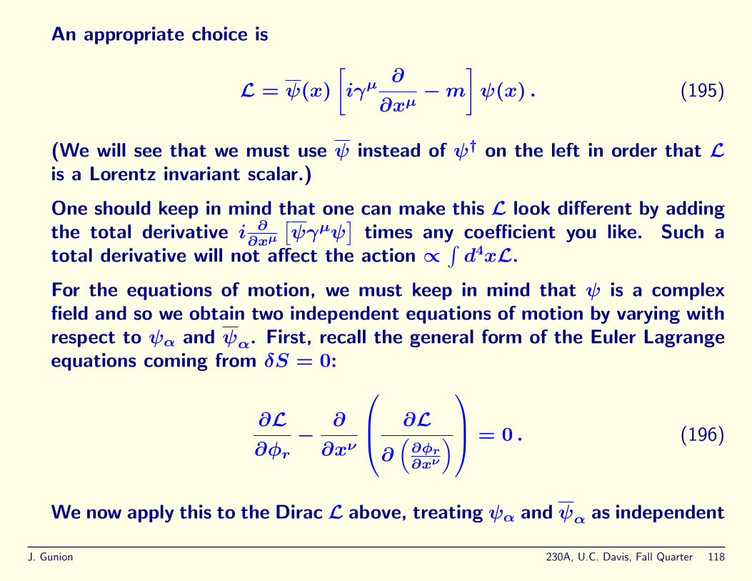
An appropriate choice is

L = ψ(x)

[iγµ

∂

∂xµ−m

]ψ(x) . (195)

(We will see that we must use ψ instead of ψ† on the left in order that Lis a Lorentz invariant scalar.)

One should keep in mind that one can make this L look different by addingthe total derivative i ∂

∂xµ

[ψγµψ

]times any coefficient you like. Such a

total derivative will not affect the action ∝∫d4xL.

For the equations of motion, we must keep in mind that ψ is a complexfield and so we obtain two independent equations of motion by varying withrespect to ψα and ψα. First, recall the general form of the Euler Lagrangeequations coming from δS = 0:

∂L∂φr−

∂

∂xν

∂L

∂(∂φr∂xν

) = 0 . (196)

We now apply this to the Dirac L above, treating ψα and ψα as independent


fields. The Dirac equation for ψα is very easily obtained by applying theEuler-Lagrange equation to the Dirac L for the case of φr = ψα:

∂L∂ψα

= 0 =

[i∂

∂xµγµαβ −m1αβ

]ψβ(x) (197)

where there is no term coming from ∂∂xν

∂L

∂

(∂ψα∂xν

) simply because (for

the particular form of L employed) there is no term in L that depends

on ∂ψα∂xν

. In the above, I have made the Dirac indices completely explicit.Making them implicit, the above is identical to the covariant form of theDirac equation given earlier.

• For 2nd quantization, we need the conjugate momentum densities of ψαand ψα. From L we have

πα(x) =∂L∂ψα

= i[ψ(x)γ0]α = i[ψ†γ0γ0]α = iψ†α

πα(x) =∂L

∂ψα

= 0 . (198)


The Hamiltonian and Momentum operators

• The Hamiltonian and momentum operators are obtained from the Noetherprocedure and take the form:

H =

∫d3~xH =

∫d3~x[πα(x)ψα(x) + πα(x)ψα(x)− L]

=

∫d3~x[iψ†(x)ψ(x)− L]

=

∫d3~x[iψ(x)γ0 ∂

∂x0ψ(x)− iψ(x)γµ

∂

∂xµψ(x) +mψ(x)ψ(x)]

=

∫d3~xψ(x)[−iγj

∂

∂xj+m]ψ(x)

P j =

∫d3~x [πα(x)

∂ψα(x)

∂xj+ 0]

=

∫d3~x [iψ†(x)(−∇j)ψ(x) i.e.

~P = −i∫d3~xψ†(x)~∇ψ(x) .


The Angular Momentum operator

• The angular momentum operator requires knowing what the generator ofrotations is for the Dirac field. To this end, we must go to Peskin andSchroeder, chapter 3.

I outline the approach.

1. First, you must understand that rotations are in general generatedby rotation operators of the form R = exp[−iθiJ i], where the J i,i = 1, 2, 3, are called the generators of the rotation group.The exact form of these generators depends upon the representation ofthe rotation group. Some examples that you know about already are:– the non-relativistic spin-1/2 generators which are the Pauli matrices:~J = ~σ/2.

– the angular momentum operator in non-relativistic quantum mechanics:~J = ~x× ~p = ~x× (−i~∇).

These operators operate on different spaces. The Pauli matrices operatein the space of two-component spinors. The NRQM angular momentumoperator operates on NRQM wave functions.


However, they have a common property; namely the commutationrelations:

[J i, Jj] = iεijkJk . (199)

These commutation relations for the group generators are what actuallyspecifies the rotation group.

2. We can generalize the NRQM rotation generators to include Lorentzboosts by using an antisymmetric tensor notation:

J ij = −i(xi∇j − xj∇i) (200)

is identified with the above Jk according to J3 = J12, and so forth.This we generalize to

Jµν = i(xµ∂ν − xν∂µ). (201)

These 6 operators generate the three boosts and three rotations of theLorentz group.

3. Using simple algebra, one finds the generalized Lorentz group commutators:

[Jµν, Jρσ] = i (gνρJµσ − gµρJνσ − gνσJµρ + gµσJνρ) . (202)


4. Another simple representation of these Jµν is that for Lorentz transformationsof the usual 4-vectors:

(J µν)αβ = i(δµαδνβ − δ

µβδνα) , (203)

where the α and β are the Lorentz indices that are connected with thevector indices on the coordinates.You can easily verify that this representation of the Jµν obeys the generalcommutator relations above that specify the group.Lorentz 4-vectors transform under infinitesimal boosts or rotations accordingto

V α ≡ ΛαβVβ → (δαβ −

i

2ωµν(J µν)αβ)V β , (204)

or equivalently

Vα→ Vα −i

2ωµν(J µν)αβV β (205)

Plugging in Eq. (203) gives

Vα→ Vα + ωαβVβ . (206)

If we look back at the transform used to define the Noether current


Eq. (79) one findsxα→ xα + εαβx

β (207)

implying that ωαβ = εαβ. This will be important shortly. For now let uslook at two examples.For example, a z-axis rotation would be specified by ω12 = −ω21 =−θR. An infinitesimal boost in the x-direction would correspond toω01 = −ω10 = −βB (the boost velocity). In both cases, I have chosenthe signs appropriate for the passive point of view. We can verifythese claims as follows. Let us consider the boost case, for which thegenerator of interest is (J 01)αβ = i(g0αδ1

β − δ0βg

1α). The antisymmetryof ω01 = −ω10 = −βB means that

−i

2ωµν(J µν)αβ = −βB(g0αδ1

β − δ0βg

1α) . (208)

Looking at the α, β = 0, 1 components of the general boost equation,we find Λ0

0 = 1, Λ01 = −βB, Λ1

0 = −βB and Λ11 = 1, where we had to

use g00 = 1 and g11 = −1. The result is(t′

x′

)=

(1 −βB−βB 1

)(tx

), (209)


which is of course correct for the visualization (passive) where you lookat some fixed physical location using the coordinates of a prime framethat is boosted with positive velocity along the x axis in the unprimedframe. Returning to the rotation example, we have

−i

2ωµν(J µν)αβ = −θR(g1αδ2

β − δ1βg

2α) (210)

and focusing on the α, β = 1, 2 components we have Λ11 = 1, Λ2

2 = 1,Λ1

2 = θR and Λ21 = −θR, yielding

(x′

y′

)=

(1 θR−θR 1

)(xy

), (211)

which describes the coordinates of a given physical point using thecoordinates defined in a new frame obtained from the old frame byrotating by an amount θR about the positive z axis (again the passivepoint of view).Of course, these infinitesimal forms can be exponentiated to give the


usual finite results. For example, in the case of the boost we would have

(t′

x′

)= exp

[(0 −βB−βB 0

)](t

x

)=

(coshβB − sinhβB− sinhβB coshβB

)(t

x

).

(212)

5. An interesting exercise is to find all the finite dimensional representationsof the Lorentz group. This we will not do in general.However, if we define n×n matrices obeying [γµ, γν]+ = 2gµν × 1n×n,then one can show that the matrices defined by

Sµν =i

4[γµ, γν] ≡

1

2σµν (213)

satisfy the Lorentz generator commutator algebra.The demonstration that the Sµν defined in this way satisfy the Lorentzgenerator commutator algebra (for any n) is assigned as a problem.Obviously the case of n = 4 is what we shall employ.

6. The form of the γµ in the Weyl representation of the Dirac matrices (thisuse of the word “representation” is not the same as the group theory


use) is

γ0 =

(0 11 0

), γi =

(0 σi

−σi 0

). (214)

For this choice, we can work out the Sµν explicitly:

S0i =i

4[γ0, γi] = −

i

2

(σi 00 −σi

)Sij =

i

4[γi, γj] =

1

2εijk

(σk 00 σk

). (215)

We will need this explicit representation later.7. A finite Lorentz transformation when working with the 4-component ψα

basis has the form

Λ1/2 = exp

(−i

2ωµνS

µν

). (216)

In a moment, it will be important to note that Λ1/2 is not a unitarymatrix for boosts, since the S0i are not Hermitian. In fact, it is easilyseen from the above explicit form of S0i that S0i is antihermitian; incontrast, the Sij are hermitian.


8. There are several very important properties of these Sρσ.(a) [γµ, Sρσ] = (J ρσ)µνγ

ν, which implies

(1 +i

2ωρσS

ρσ)γµ(1−i

2ωρσS

ρσ) = (1−i

2ωρσJ ρσ)µνγ

ν (217)

which is just the infinitesimal form of

Λ−11/2γ

µΛ1/2 = Λµνγν . (218)

(b) Using these results, one can show that the Dirac equation is Lorentzcovariant (takes the same form in different frames).

(c) It also allows us to see why we must use ψ rather than ψ† in writing theDirac field Lagrangian if the Lagrangian is to be a Lorentz invariant.In particular, consider the form ψ†ψ (which, multiplies m in L). Undera Lorentz transformation, ψ†ψ → ψ†Λ†1/2Λ1/2ψ. However, Λ1/2 is nota unitary matrix in the case of boosts for which the generators are notHermitian. The trick is to note that the Sij are hermitian whereasthe S0i are antihermitian ((S0i)† = −S0i) and that γ0Sij = +Sijγ0

whereas γ0S0i = −S0iγ0.


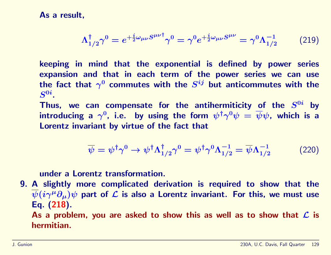
As a result,

Λ†1/2γ0 = e+ i

2ωµνSµν†γ0 = γ0e+ i

2ωµνSµν

= γ0Λ−11/2 (219)

keeping in mind that the exponential is defined by power seriesexpansion and that in each term of the power series we can usethe fact that γ0 commutes with the Sij but anticommutes with theS0i.Thus, we can compensate for the antihermiticity of the S0i byintroducing a γ0, i.e. by using the form ψ†γ0ψ = ψψ, which is aLorentz invariant by virtue of the fact that

ψ = ψ†γ0 → ψ†Λ†1/2γ0 = ψ†γ0Λ−1

1/2 = ψΛ−11/2 (220)

under a Lorentz transformation.9. A slightly more complicated derivation is required to show that theψ(iγµ∂µ)ψ part of L is also a Lorentz invariant. For this, we must useEq. (218).As a problem, you are asked to show this as well as to show that L ishermitian.


So, finally we are able to derive what the angular momentum operator isusing the infinitesimal form of Λ1/2. We have:

ψα(x)→ ψ′α(x′) = ψα(x)−i

2ωµνS

µναβψβ(x)

= ψα(x)−i

4εµνσ

µναβψβ(x) ,

(221)

where the last equation is written in the notation of Mandl and Shaw, i.e.we used ωµν = εµν, and we used Eq. (213). This is now in the formrequired for obtaining the conserved current from the Noether theorem.

• The Noether current for the angular momentum operator.

Recall that for xµ → x′µ = xµ + εµνxν, the Noether current depended

upon the matrix appearing in

φr(x)→ φ′r(x′) = φr(x) +

1

2εµνS

µνrs φs(x) (222)

(where of course we think of the φr as being the ψα in the present Dirac


situation). Comparing Eq. (221) and Eq. (222), we see that

Sµνrs → −i

2σµν . (223)

This appeared in the angular momentum operator in the form

Mµν =

∫d3~x

[xµT 0ν − xνT 0µ] + πr(x)Sµνrs φs(x)

. (224)

Now, for discussing angular momentum and spin, we are only interested inthe spatial coordinates, µ, ν = i, j. In this case, we write

M ij =

∫d3~x

xiT 0j − xjT 0i + πr(x)Sijrsφs(x)

, (225)

where T 0j(x) = Pj(x) = πr(x)∂φr(x)∂xj

is the general result, where we

sum over all the fields in the r, s sums. (In the above Pj(x) is themomentum density, the integral of which gives the 3-momentum givenearlier in Eq. (199).) Now, in the Dirac case, this sum over fields andtheir conjugate momenta includes both ψα (recall that the Dirac field


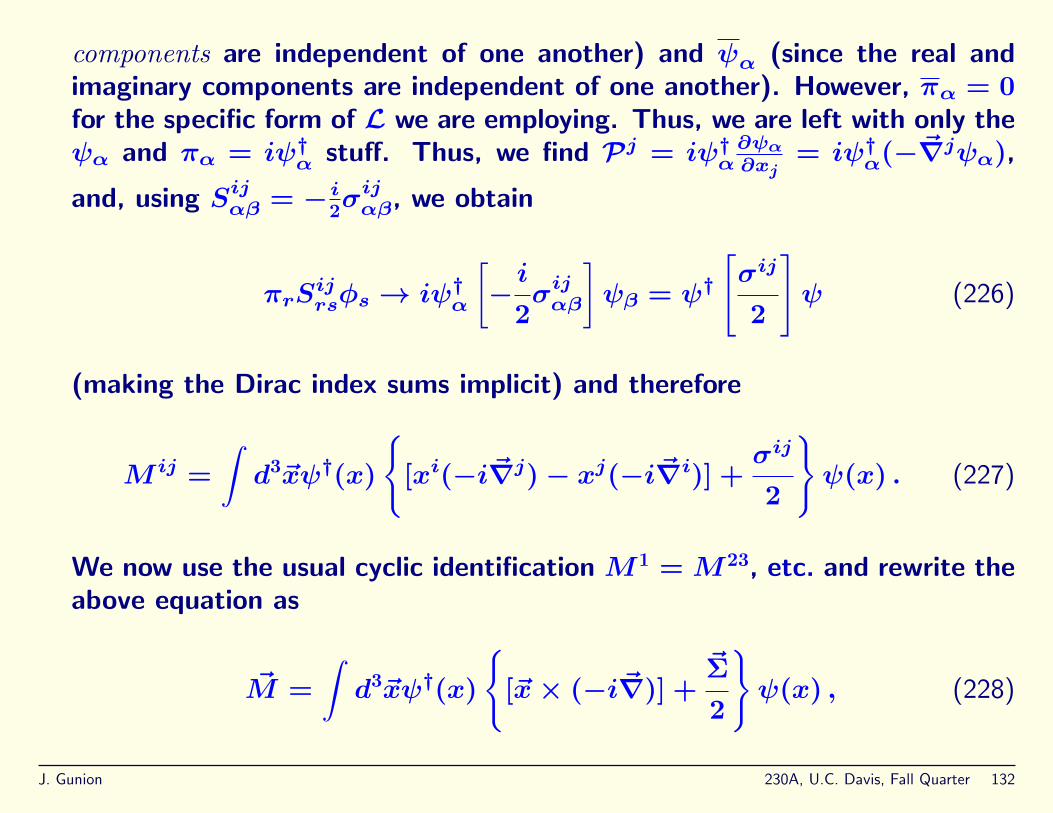
components are independent of one another) and ψα (since the real andimaginary components are independent of one another). However, πα = 0for the specific form of L we are employing. Thus, we are left with only theψα and πα = iψ†α stuff. Thus, we find Pj = iψ†α

∂ψα∂xj

= iψ†α(−~∇jψα),

and, using Sijαβ = −i2σijαβ, we obtain

πrSijrsφs→ iψ†α

[−i

2σijαβ

]ψβ = ψ†

[σij

2

]ψ (226)

(making the Dirac index sums implicit) and therefore

M ij =

∫d3~xψ†(x)

[xi(−i~∇j)− xj(−i~∇i)] +

σij

2

ψ(x) . (227)

We now use the usual cyclic identification M1 = M23, etc. and rewrite theabove equation as

~M =

∫d3~xψ†(x)

[~x× (−i~∇)] +

~Σ

2

ψ(x) , (228)


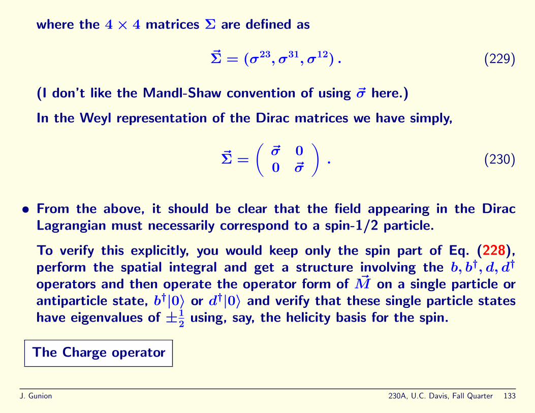
where the 4× 4 matrices Σ are defined as

~Σ = (σ23, σ31, σ12) . (229)

(I don’t like the Mandl-Shaw convention of using ~σ here.)

In the Weyl representation of the Dirac matrices we have simply,

~Σ =

(~σ 00 ~σ

). (230)

• From the above, it should be clear that the field appearing in the DiracLagrangian must necessarily correspond to a spin-1/2 particle.

To verify this explicitly, you would keep only the spin part of Eq. (228),perform the spatial integral and get a structure involving the b, b†, d, d†

operators and then operate the operator form of ~M on a single particle orantiparticle state, b†|0〉 or d†|0〉 and verify that these single particle stateshave eigenvalues of ±1

2using, say, the helicity basis for the spin.

The Charge operator


• Since L is invariant under a phase rotation of the complex field, ψ → eiφψ(which implies ψ → e−iφψ), the Noether procedure leads to a conservedcharge current. The general equation

Q = −iq∫d3~x[πr(x)φr(x)− π†r(x)φ†r(x)] (231)

reduces in the present Dirac case to

Q = −iq∫d3~x[πα(x)ψα(x)− 0]

= −iq∫d3~x[iψ†α(x)ψα(x)] = q

∫d3~xψ†(x)ψ(x) ,

and the corresponding charge-current density is

jµ = (ρ(x),~j(x)) = qψ(x)γµψ(x) . (232)

One can explicitly check that ∂jµ

∂xµ= 0 follows by use of the Dirac equation

for the ψ and ψ fields.


• You may recall that Dirac actually wanted to have ψ†ψ = ψγ0ψ be positivedefinite since it looked to him like a probability density. Thus, we havecome 180; our Lagrangian + Noether theorem implies that this must bethe charge density, with opposite sign for particles vs. antiparticles. Thiswe will see explicitly when we 2nd quantize.

The plane wave solutions of the Dirac equation

• To 2nd quantize the Dirac field, we need a complete set of solutions to theDirac equation. This is closely analogous to what we did for ~A and for φ,where we expanded in terms of solutions of the KG equation or of 2 ~A = 0.

We then 2nd quantize by turning the c-number expansion coefficients intooperators. In the Dirac case, we will demand that these operator coefficientsobey anticommutation quantization conditions.

• Since the Dirac wave function has four components, and since we saw inthe KG case that plane waves come in the form eip·x and e−ip·x, we cananticipate that the complete set will look like

ur(~p)e−ip·x√V

, vr(~p)e+ip·x√V

, r = 1, 2 , (233)


where p0 = E~p ≡√m2 + ~p2 is the 0th component of the 4-vector p.

• If these are plane wave solutions, they must obey(i∂

∂xµγµ −m

)ur(~p)e−ip·x = (p/ −m)ur(~p)e−ip·x = 0(

i∂

∂xµγµ −m

)vr(~p)e+ip·x = (−p/ −m)vr(~p)e+ip·x = 0

where we employ the notation v/ = vµγµ.

In fact, ur and vr must obey the equations

(p/ −m)ur(~p) = 0 , (p/ +m)vr(~p) = 0 (234)

without the exponents in order that the Dirac equation plane waves obeythe Dirac equation for any x.

• ur and vr are called the positive and negative energy solutions by Dirac,and we will often use this language, but really they are the particle andantiparticle solutions, as we shall see.


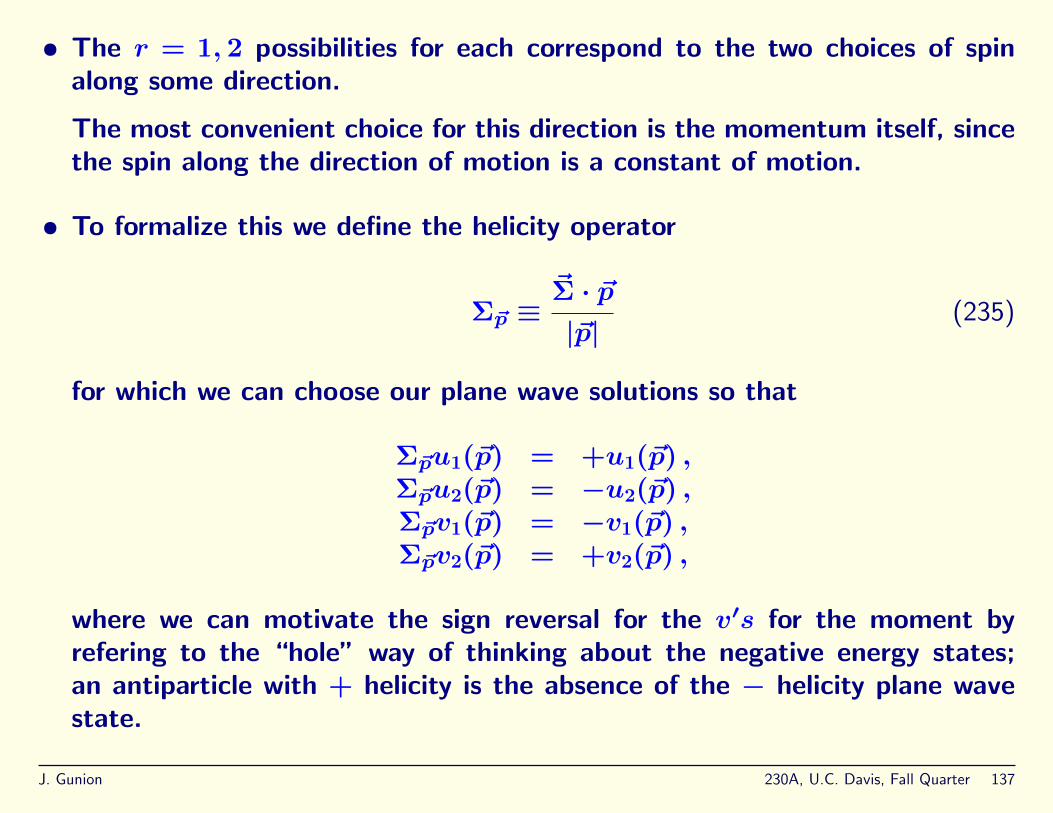
• The r = 1, 2 possibilities for each correspond to the two choices of spinalong some direction.

The most convenient choice for this direction is the momentum itself, sincethe spin along the direction of motion is a constant of motion.

• To formalize this we define the helicity operator

Σ~p ≡~Σ · ~p|~p|

(235)

for which we can choose our plane wave solutions so that

Σ~pu1(~p) = +u1(~p) ,Σ~pu2(~p) = −u2(~p) ,Σ~pv1(~p) = −v1(~p) ,Σ~pv2(~p) = +v2(~p) ,

where we can motivate the sign reversal for the v′s for the moment byrefering to the “hole” way of thinking about the negative energy states;an antiparticle with + helicity is the absence of the − helicity plane wavestate.


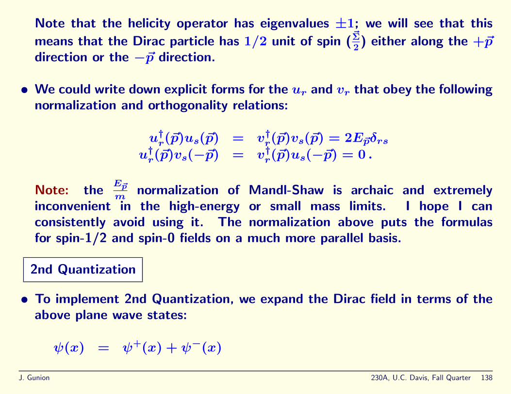
Note that the helicity operator has eigenvalues ±1; we will see that this

means that the Dirac particle has 1/2 unit of spin (~Σ2

) either along the +~pdirection or the −~p direction.

• We could write down explicit forms for the ur and vr that obey the followingnormalization and orthogonality relations:

u†r(~p)us(~p) = v†r(~p)vs(~p) = 2E~pδrsu†r(~p)vs(−~p) = v†r(~p)us(−~p) = 0 .

Note: theE~pm

normalization of Mandl-Shaw is archaic and extremelyinconvenient in the high-energy or small mass limits. I hope I canconsistently avoid using it. The normalization above puts the formulasfor spin-1/2 and spin-0 fields on a much more parallel basis.

2nd Quantization

• To implement 2nd Quantization, we expand the Dirac field in terms of theabove plane wave states:

ψ(x) = ψ+(x) + ψ−(x)


=∑r,~p

(1

2V E~p

)1/2 [cr(~p)ur(~p)e−ip·x + d†r(~p)vr(~p)e+ip·x] .

The conjugate field ψ = ψ†γ0 will then have the expansion

ψ(x) = ψ+

(x) + ψ−

(x)

=∑r,~p

(1

2V E~p

)1/2 [dr(~p)vr(~p)e−ip·x + c†r(~p)ur(~p)e+ip·x] ,

where we have defined ur ≡ u†rγ0, . . ..

In all of this, we are temporarily using a finite volume for which the momentawill take on the usual discrete values.

We have written c†r instead of c∗r, and d†r instead of d∗r in anticipation ofthese becoming operators as part of 2nd quantization.

• Quantize using anticommutators. We will see later that this is required bycausality.

[cr(~p), c†s(~k)]+ = [dr(~p), d†s(

~k)]+ = δrsδ~p~k (236)


with all other anticommutators equal to zero.

• Define the vacuum by

cr(~p)|0〉 = dr(~p)|0〉 = 0, all ~p, and r=1,2 . (237)

• Define the number operators

Nr(~p) = c†r(~p)cr(~p) , Nr(~p) = d†r(~p)dr(~p) . (238)

• From the above, we can show that it is consistent to think of cr and dras being particle and antiparticle annihilation operators, c†r and d†r as beingthe corresponding creation operators, where Nr and Nr are the numberoperators for particles and antiparticles, respectively

• But, we must check the other physical properties of the particles by lookingfor the constants of motion (conserved quantities) and seeing that they aresensible quantities related to what we expect for properties of particles.


• In computing these constants of motion, we will naturally measure thingslike energy, momentum and charge relative to the vacuum state if we, fromthe beginning, just employ the normal ordering prescription.

But, for fermions, we need to modify our definition just slightly to accountfor the anticommutation of the operators.

In arranging operators in the Bose case, we reordered assuming that allcommutators vanished. In the Dirac case, we will reorder assuming allanticommutators vanish.

: ψαψβ : = : (ψ+α + ψ−α )(ψ+

β + ψ−β ) :

= ψ+αψ

+β − ψ

−β ψ

+α + ψ−αψ

+β + ψ−αψ

−β .

• So now we compute the constants of motion obtained earlier from thesymmetries of the Dirac L, incorporating the normal ordering prescription,e.g.

H =

∫d3~x : ψ(x)

[−iγj

∂

∂xj+m

]ψ(x) : . (239)


• We must repeatedly use the orthonormality properties for the plane waves.We obtain:

H =∑r~p

E~p[Nr(~p) +Nr(~p)] (240)

~P =∑r~p

~p[Nr(~p) +Nr(~p)] (241)

Q = −e∑r~p

[Nr(~p)−Nr(~p)] (242)

where in the last equation we have adopted the usual convention in whichthe particle of the system is identified as the electron with charge −e,where e > 0.

Because we will need the pre-normal-ordered version of H later (to discussthe spin-statistics connection), let us derive the form of H. The steps are(without normal ordering):

H =

∫d

3~xψ(x)[−iγj∂j +m]ψ(x)

=

∫d

3~x∑~p,r

1√2V E~p

∑~k,s

1√2V E~k

(dr(~p)vr(~p)e

−ip·x+ c†r(~p)ur(~p)e

ip·x)×


[−iγj∂j +m](cs(~k)us(~k)e

−ik·x+ d†s(~k)vs(~k)e

ik·x)

=

∫d

3~x∑~p,r

1√2V E~p

∑~k,s

1√2V E~k

(dr(~p)vr(~p)e


ip·x)×

(cs(~k)((−i)(−i)γjkj +m)us(~k)e

−ik·x+ d†s(~k)((−i)(+i)γjkj +m)vs(~k)e

ik·x)

=

∫d

3~x∑~p,r

1√2V E~p

∑~k,s

1√2V E~k

(dr(~p)vr(~p)e


ip·x)×

(cs(~k)(+k

0γ

0)us(~k)e

−ik·x+ d†s(~k)(−k0

γ0))vs(~k)e

ik·x)

=∑~p,r

1√2V E~p

∑~k,s

1√2V E~k

V

[dr(~p)cs(~k)vr(~p)E~kγ

0us(~k)δ

~p,−~ke−2iE~k

x0

+c†r(~p)cs(~k)ur(~p)(E~kγ

0)us(~k)δ

~p,~k

+dr(~p)d†s(~k)vr(~p)(−E~kγ

0)vs(~k)δ

~p,~k

+c†r(~p)d

†s(~k)ur(~p)(−E~kγ

0)vs(~k)δ

~p,−~ke+2iE~k

x0]

=1

2

∑~p,r,s

[dr(~p)cs(−~p)vr(~p)γ

0us(−~p)e

−2iE~px0

+ c†r(~p)cs(~p)ur(~p)γ

0us(~p)

−dr(~p)d†s(~p)vr(~p)γ

0vs(~p)− c†r(~p)d

†s(−~p)ur(~p)γ

0vs(−~p)e

+2iE~px0]


=1

2

∑~p,r,s

[dr(~p)cs(−~p)(0)e

−2iE~px0

+ c†r(~p)cs(~p)2E~pδrs

−dr(~p)d†s(~p)2E~pδrs − c

†r(~p)d

†s(−~p)(0)e

+2iE~px0]

=∑~p,r

E~p

[c†r(~p)cr(~p)− dr(~p)d

†r(~p)

](243)

where we used

(k/ −m)u(~k) = (γ0k0 + γ

jkj −m)u(~k) = 0 , ⇒ (−γjkj +m)u(~k) = γ

0k

0u(~k) ,(244)

(k/ +m)v(~k) = (γ0k0 + γ

jkj +m)v(~k) = 0 , ⇒ (γ

jkj +m)v(~k) = −γ0

k0v(~k) .(245)

and the orthonormal properties outlined earlier of the spinors outlined earlier:

ur(~p)γ0us(~p) = u

†r(~p)us(~p) = 2E~pδrs (246)

vr(~p)γ0vs(~p) = v

†r(~p)vs(~p) = 2E~pδrs (247)

vr(~p)γ0us(−~p) = v

†r(~p)us(−~p) = 0 (248)

ur(~p)γ0vs(−~p) = u

†r(~p)vs(−~p) = 0 . (249)

You are assigned the problem of showing that Q is given by the equationEq. (242), following similar procedures to the H derivation above.

• The last item on the list is the spin operator. We employ the helicity


(longitudinal spin in the words of Mandl-Shaw) operator which is the non-angular-momentum part of the total angular momentum operator we wrotedown from the rotational symmetry of L:

S~p =1

2

∫d3~x : ψ†(x)Σ~pψ(x) : , (250)

from which one finds by direct computation

S~pc†r(~p)|0〉 = (−1)r+11

2c†r(~p)|0〉 , (251)

S~pd†r(~p)|0〉 = (−1)r+11

2d†r(~p)|0〉 , (252)

which is to say that the r = 1 states for both the particle and antiparticlehave +1/2 helicity, while the r = 2 states have −1/2 helicity.

The “flip” of the antiparticle projection helicity relative to the simpleresult of Σ~p operating on the vr states comes about as a result of theanticommutations that emerge in the above computations. Let us checkthis.


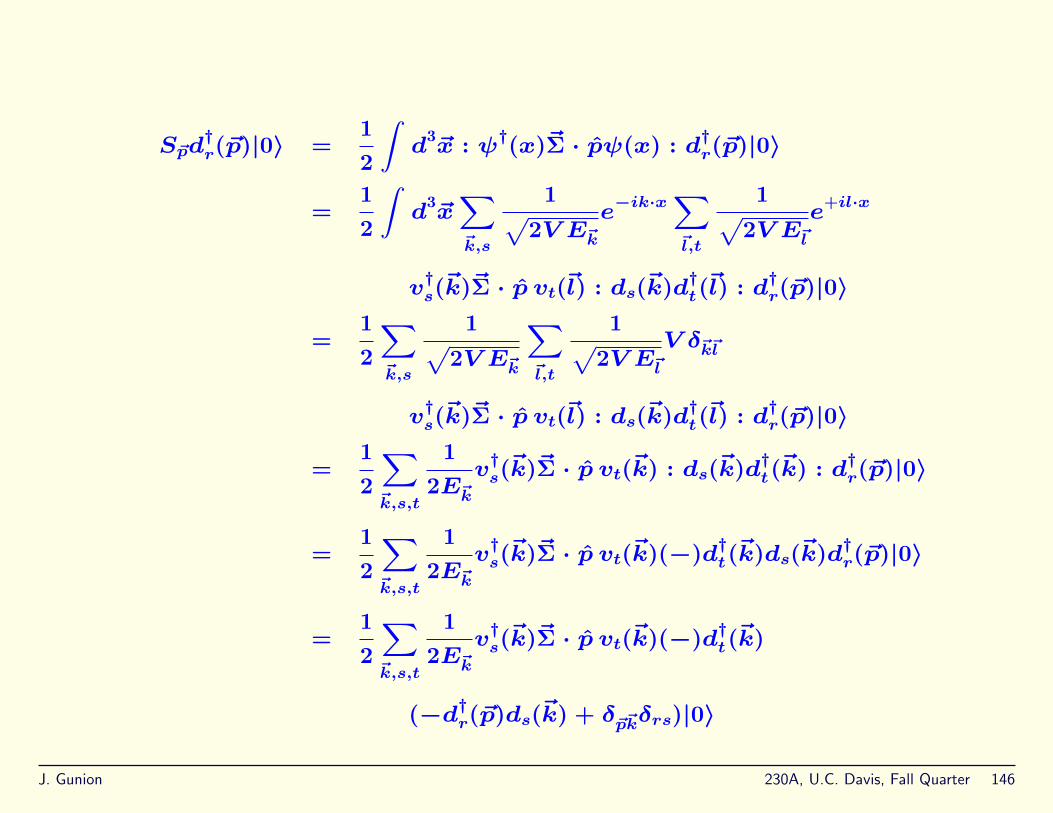
S~pd†r(~p)|0〉 =

1

2

∫d

3~x : ψ

†(x)~Σ · pψ(x) : d

†r(~p)|0〉

=1

2

∫d

3~x∑~k,s

1√2V E~k

e−ik·x∑

~l,t

1√2V E~l

e+il·x

v†s(~k)~Σ · p vt(~l) : ds(~k)d

†t(~l) : d

†r(~p)|0〉

=1

2

∑~k,s

1√2V E~k

∑~l,t

1√2V E~l

V δ~k~l

v†s(~k)~Σ · p vt(~l) : ds(~k)d

†t(~l) : d

†r(~p)|0〉

=1

2

∑~k,s,t

1

2E~kv†s(~k)~Σ · p vt(~k) : ds(~k)d

†t(~k) : d

†r(~p)|0〉

=1

2

∑~k,s,t

1

2E~kv†s(~k)~Σ · p vt(~k)(−)d

†t(~k)ds(~k)d

†r(~p)|0〉

=1

2

∑~k,s,t

1

2E~kv†s(~k)~Σ · p vt(~k)(−)d

†t(~k)

(−d†r(~p)ds(~k) + δ~p~kδrs)|0〉


=1

2

∑t

1

2E~pv†r(~p)~Σ · p vt(~p)(−)d

†t(~p)|0〉

=1

2

∑t

1

2E~pv†r(~p)(−1)

tvt(~p)(−)d

†t(~p)|0〉

=1

2

∑t

1

2E~p(−1)

t2E~pδrt(−)d

†t(~p)|0〉

=1

2(−1)

r+1d†r(~p)|0〉 (253)

Can you justify all the steps? There is one little detail that I sort of slippedin. In principle, what you should actually do is compute ~Jop · ~Popd†r(~p)|0〉.But, of course ~p pops out, giving you ~Jop · ~p = .... There is anotherway that should be equivalent. That is to employ the helicity density~J (x) · ~P(x) (each being the appropriate bilinear form), integrated over∫d3~x and operate this on d†r(~p). This should give the same answer but is

a far harder computation.

• Thus the particles and antiparticles of the theory have all the same propertiesexcept for the sign of the charge, as required for the use of the words particleand antiparticle.


The Majorana representation of the Dirac matrices

• To make the symmetry between antiparticles and particles more apparent,one would use a particular representation of the γ matrices, the “Majorana”representation which has the property:

γµ ∗M = −γµM , µ = 0, 1, 2, 3 (254)

where the ∗ denotes simple complex conjugation. In other words, in theMajorana rep. all four γ matrices are pure imaginary. Explicit forms of theγM that also obey the anticommutation relations for the γ matrices aregiven in the Appendix of Mandl-Shaw, for example.

• In the Majorana representation, the Dirac operator(iγµM

∂

∂xµ−m

)(255)

is real. Hence, if ψM is a solution of the dirac equation in a Majoranarepresentation, so is its complex conjugate ψ∗M .


It follows that if the positive energy solutions are denoted by

uMr(~p)e−ip·x√V

, (256)

in the Majorana representation, then the corresponding negative energysolutions are

u∗Mr(~p)eip·x√V. (257)

Proof:

0 =

[(iγµM

∂

∂xµ−m

)uMr(~p)e−ix·p

]∗=

[(p/ −m)uMr(~p)e−ix·p

]∗= (−p/ −m)u∗Mr(~p)e+ix·p

=

(iγµM

∂

∂xµ−m

)u∗Mr(~p)e+ix·p ,

where we, of course, used p/ ∗ = −p/ in the Majorana representation.


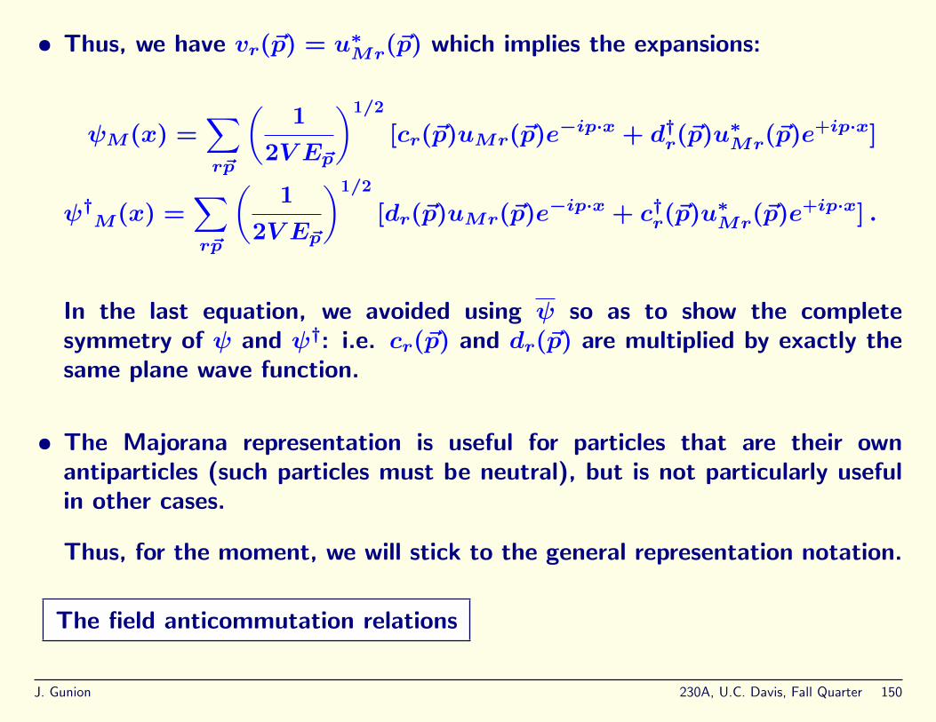
• Thus, we have vr(~p) = u∗Mr(~p) which implies the expansions:

ψM(x) =∑r~p

(1

2V E~p

)1/2

[cr(~p)uMr(~p)e−ip·x + d†r(~p)u∗Mr(~p)e+ip·x]

ψ†M(x) =∑r~p

(1

2V E~p

)1/2

[dr(~p)uMr(~p)e−ip·x + c†r(~p)u∗Mr(~p)e+ip·x] .

In the last equation, we avoided using ψ so as to show the completesymmetry of ψ and ψ†: i.e. cr(~p) and dr(~p) are multiplied by exactly thesame plane wave function.

• The Majorana representation is useful for particles that are their ownantiparticles (such particles must be neutral), but is not particularly usefulin other cases.

Thus, for the moment, we will stick to the general representation notation.

The field anticommutation relations


• Starting from the anticommutator algebra for the c, c†, d, d†, one can“easily” show that

[ψα(x), ψβ(y)]+ = [ψα(x), ψβ(y)]+ = 0 (258)

[ψ±α (x), ψ∓β (y)]+ = i

(iγµ

∂

∂xµ+m

)αβ

∆±(x− y) = iS±αβ(x− y) ,

(259)

where the ∆±(x) are the invariant ∆-functions encountered in our studyof the KG equation, except that they are defined using mass m of theDirac particle rather than some other unrelated mass µ of a Klein Gordonparticle. You are assigned the problem of verifying Eq. (259).

• Using the above two equations we obtain easily

[ψ(x), ψ(y)]+ = iS(x− y) (260)

where we define, using ∆(x) = ∆+(x) + ∆−(x) from KG results,

S(x) ≡ S+(x)+S−(x) =

(iγµ

∂

∂xµ+m

)∆(x) ≡ (i∂/+m)∆(x) (261)


where Dirac matrix indices are implicit.

• It is thought-provoking to use this result to compute the equal timeanticommutator

[ψ(~x, t), ψ(~y, t)]+ =

[(iγµ

∂

∂xµ+m

)∆(x− y)

]x0=y0=t

. (262)

One way of proceeding is to recall that ∆(x−y) = [φ(x), φ(y)] (φ being areal scalar field) and that [φ(x), φ(y)]x0=y0 = −iδ3(~x−~y) was the definingequal time commutator for the scalar field 2nd quantization.

Now, since the iγi ∂∂xi

+m part of the operator above does not involve thetime derivative we have[(iγi

∂

∂xi+m

)[φ(x), φ(y)]

]x0=y0

=

(iγi

∂

∂xi+m

)[φ(x), φ(y)]x0=y0

=

(iγi

∂

∂xi+m

)0

= 0 (263)


where [φ(x), φ(y)]x0=y0 = 0 comes from the fact that the fields commutefor space like separations.

Thus, we are left only with the time derivative piece:[iγ0 ∂

∂x0[φ(x), φ(y)]

]x0=y0

= iγ0[φ(x), φ(y)]x0=y0

= iγ0[−iδ3(~x− ~y)

]= γ0δ3(~x− ~y) . (264)

Of course, remembering that ψ(y) = ψ†(y)γ0, our result can be rewritten(displaying the previously implicit Dirac indices explicitly) as:

[ψα(~x, t), ψ†β(~y, t)]+ = δαβδ3(~x− ~y) . (265)

If we recall that πα(y) = iψ†α, the above gives

[ψα(~x, t), πβ(~y, t)]+ = iδαβδ3(~x− ~y) . (266)

This is the exact analogue of the 2nd quantization we used for the scalarfield case. The only difference is that for the Dirac field we have employed


the anticommutator instead of the commutator. In short, an equivalentway to get at the anticommutator quantization rules for the c, d, c†, d†

operators would have been to require Eq. (266).

• This brings up the question of normalizations. Just as discussed in the scalarfield case, there is a certain arbitrariness in the normalizations employedwhen writing

ψ(x) =∑r,~p

(1

2V E~p

)1/2 [cr(~p)ur(~p)e−ip·x + d†r(~p)vr(~p)e+ip·x] (267)

and in the [cr(~p), c†r(~k)]+ = δ~p~k , . . . anticommutators. Keeping the same

normalization convention for the spinors ur and vr, we could still change

the(

12V E~p

)1/2

factor to f1/2 (say) times this while retaining Eq. (266)

(which has the standard 2nd quantization normalization) provided we makea compensating change in the normalization of the Foch space c, d, c†, d†

anticommutators to have an extra factor of 1/f .

At the same time, you must consider what would happen to the form of


H. You would find that

H =∑~p,r

fE~p[Nr(~p) +Nr(~p)

]. (268)

(Here, we retain the definitions

Nr(~p) = c†r(~p)cr(~p) , Nr(~p) = d†r(~p)dr(~p) (269)

employed earlier.) One would then compute

H|~k, s〉 = Hc†s(~k)|0〉 = E~k|~k, s〉 , (270)

where the last equality comes from using the new rescaled anticommutators(including the extra 1/f factor, which cancels the extra f in the expressionfor H). So, such rescalings do not affect the fact that the Hamiltonianoperator gives the correct result for the energy of a single particle state.

At this point, you should ask about the normalization of our starting L,since it was this normalization that determined the normalization of H.(Note that L could be multiplied by an arbitrary constant without changing


the equation of motion for ψ.) In fact, we chose the normalization of L sothat the normalization of the H and ~P operators corresponded to our usualconventions for defining what we mean by energy and momentum. This isreferred to as “canonical normalization”. It will always be important to referto canonical normalization when defining what we mean by the canonicallynormalized fields that define the particles (the physical eigenstates) of ourtheory. This seemingly trivial remark can have some profound implicationsonce interactions and mixings between particles are incorporated into ourtheory.

• Starting from the contour integral representations of the ∆±, we easilyobtain from Eq. (259) that

S±(x) = −1

(2π)4

∫C±

d4p e−ip·xp/ +m

p2 −m2, (271)

where the C± contours are the anticlockwise paths enclosing the poles atp0 = ±E~p.

Since (p/ ±m)(p/ ∓m) = p2 −m2, the last equation can be abbreviated


in the form

S±(x) = −1

(2π)4

∫C±

d4p e−ip·x1

p/ −m, (272)

Note:

a/ a/ = aµaνγµγν

= aµaν1

2[γµγν + γνγµ] = aµaν

1

2[2gµν] = a · a . (273)

Discussion on spin-statistics connection

• We can ask what would have happened had we quantized the Dirac systemusing commutators instead of anticommutators.

At the first level, i.e. directly from the expression for H and the fieldexpansion forms but before assuming commutation or anticommutation,one obtains

H =∑r~p

E~p[c†r(~p)cr(~p)− dr(~p)d†r(~p)] . (274)


If we employ anticommutation, then we can rewrite the 2nd term as(roughly) dd† = −d†d+ 1 to obtain

H =∑r~p

E~p[c†r(~p)cr(~p) + d†r(~p)dr(~p)− 1]

=∑r~p

E~p[Nr(~p) +Nr(~p)]−∞ . (275)

However, had we chosen to use commutation relations, we would have touse dd† = d†d+ 1, yielding

H =∑r~p

E~p[c†r(~p)cr(~p)− d†r(~p)dr(~p)− 1]

=∑r~p

E~p[Nr(~p)−Nr(~p)]−∞ . (276)

In both cases, we throw away the ∞ to define the 0 of energy andthen consider excitations relative to this. From the later result, we seethat we could have eigenstates with arbitrarily negative energy (sinceNr = 0, 1, 2, . . . are all possible in the commutation case) relative to


the vacuum state. If we want a state of lowest energy, we must useanticommutators.

• Similarly, we can ask what would happen if we quantized the KG case usinganticommutators. Here, even more bizarre things take place.

At the first stage, i.e. before assuming commutation or anticommutation,for the real field case, one finds

H =∑~p

1

2ω~p[a

†(~p)a(~p) + a(~p)a†(~p)] . (277)

Assuming commutation, we write aa† = a†a+ 1, and find

H =∑~p

ω~p[a†(~p)a(~p) +

1

2] =

∑~p

ω~p[N(~p) +1

2] . (278)

We would throw away the ∞ from the 12

and obtain the usual result.


Assuming anticommutation, we would write aa† = −a†a+ 1 and get

H =∑~p

ω~p[1

2] ; (279)

i.e. there would be no number operator in the expression for H!. The samesort of thing happens in the charged scalar field case.

Causality and the spin-statistics connection

• In the scalar field case, we verified that [φ(x), φ(y)] = 0 for space-likeseparation (x − y)2 < 0. Obviously any construct from φ(x) wouldcommute with any other construct from φ(y) for (x− y)2 < 0.

Had we tried to quantize using anticommutators, we would have found[φ(x), φ(y)] 6= 0 for (x− y)2 < 0. Mandl-Shaw says that it would be ok ifjust [φ(x), φ(y)]+ = 0 for (x− y)2 < 0. This is incorrect. There are manyobservables in nature that are linear in φ and so it is not sufficient thatbilinears in φ commute. In any case, one would find using anticommutationthat [φ(x), φ(y)]+ 6= 0 as well.


• In the Dirac field case, it is sufficient that

[ψ(x), ψ(y)]+ = [ψ(x), ψ(y)]+ = [ψ(x), ψ(y)]+ = 0 (280)

for (x− y)2 < 0 and any choice of Dirac indices (suppressed above) on thetwo fields. This is because, in the Dirac field case, for the observables tobe scalar constructs in the Dirac indices they must be bilinears of the formOi(x) = ψ(x)Γiψ(x), where, in fact, there are precisely 16 independentΓi (simply the number of independent 4× 4 matrices).

Causality will be obeyed if

[Oi(x),Oj(y)] = 0 (281)

for all choices of i, j = 1, . . . , 16 when (x− y)2 < 0.

Homework: Show that this is the case given Eq. (280). Problem 4.3 ofMandl-Shaw is a special case of this general result.

The only possibly non-zero anticommutator above is

[ψ(x), ψ(y)]+ = iS(x− y) = (i∂/ +m)∆(x− y) (282)


[see Eq. (261)] which is 0 for (x − y)2 < 0 since ∆(x − y) is 0 for(x− y)2 < 0.

Had we quantized the Dirac theory using commutators, not only would wehave ended up with energies unbounded from below, but also we would nothave been able to get causality (without the bizarre manipulations of Peskinand Schroeder, which end up violating the positive norm requirement forsingle particle states).

The Fermion Feynman propagator

• We define the fermion Feynman propagator as

〈0|Tψ(x)ψ(x′)|0〉 , (283)

where the spinor indices on the fermionic fields are not written. Like normalordering, the T instruction for fermionic fields is defined by including anextra − sign when two fermi fields are passed by one another:

Tψ(x)ψ(x′) = θ(t− t′)ψ(x)ψ(x′)− θ(t′ − t)ψ(x′)ψ(x) .(284)


where we used the earlier result:

∆F (x) = θ(t)∆+(x)− θ(−t)∆−(x) , (288)

and the fact that when the iγ0∂0 part of i∂/ acts on the time thetafunctions one obtains iγ0 times

δ(t)∆+(x) + δ(−t)∆−(x) = δ(t)∆(x) = 0 (289)

by virtue of the fact that ∆(x) is zero for space like x.

• Given Eq. (287), and the contour representation of ∆F derived earlier, wehave

SF (x) =1

(2π)4

∫d4pe−ip·x

p/ +m

p2 −m2 + iε, (290)

where the +iε in the denominator once again instructs us to pass belowthe −E~p pole and above the +E~p pole in the p0 complex plane.

• To show that this is, indeed, a Green’s function, we need to verify that(i∂/ −m)SF (x) = δ4(x). This can be done in two ways.


1. Operate on the form given in Eq. (290). Using the fact that

i∂/ e−ip·x = iγµ∂

∂xµe−ipµx

µ= (iγµ)× (−ipµ)e−ip·x = p/ e−ip·x ,

(291)and p/ p/ = p2, we obtain

(i∂/ −m)SF (x) =1

(2π)4

∫d4pe−ip·x

(p/ −m)(p/ +m)

p2 −m2 + iε

=1

(2π)4

∫d4pe−ip·x

(p2 −m2)

p2 −m2 + iε

=1

(2π)4

∫d4pe−ip·x = δ4(x) . (292)

2. Alternatively, we can note that

(i∂/ −m)SF (x) = (i∂/ −m)(i∂/ +m)∆F (x)

= (−∂/ ∂/ −m2)∆F (x)

= −(2 +m2)∆F (x)


= (−)2δ4(x) , (293)

using the fact that ∆F (x) is the Green’s function for the Klein Gordonoperator (taking care with the sign in (2 +m2)∆F (x) = −δ4(x) — seethe earlier material on ∆F — and remembering that ∆F used here isdefined with mass m of the Dirac particle).

• Analogously to the spin-0 discussion, SF (x1−x2) = 〈0|Tψ(x1)ψ(x2)|0〉incorporates simultaneously two processes:

1. For t1 > t2, an electron is emitted or created at location x2 and thenabsorbed later at x1.

2. For t2 > t1, a positron is emitted or created at location x1 and laterabsorbed at x2.

(Recall that ψ creates a e− and annihilates a e+, while ψ does the reverse.)

Interactions with the electromagnetic field

• Problem 1.2 introduced you to the minimal substitution interaction, which


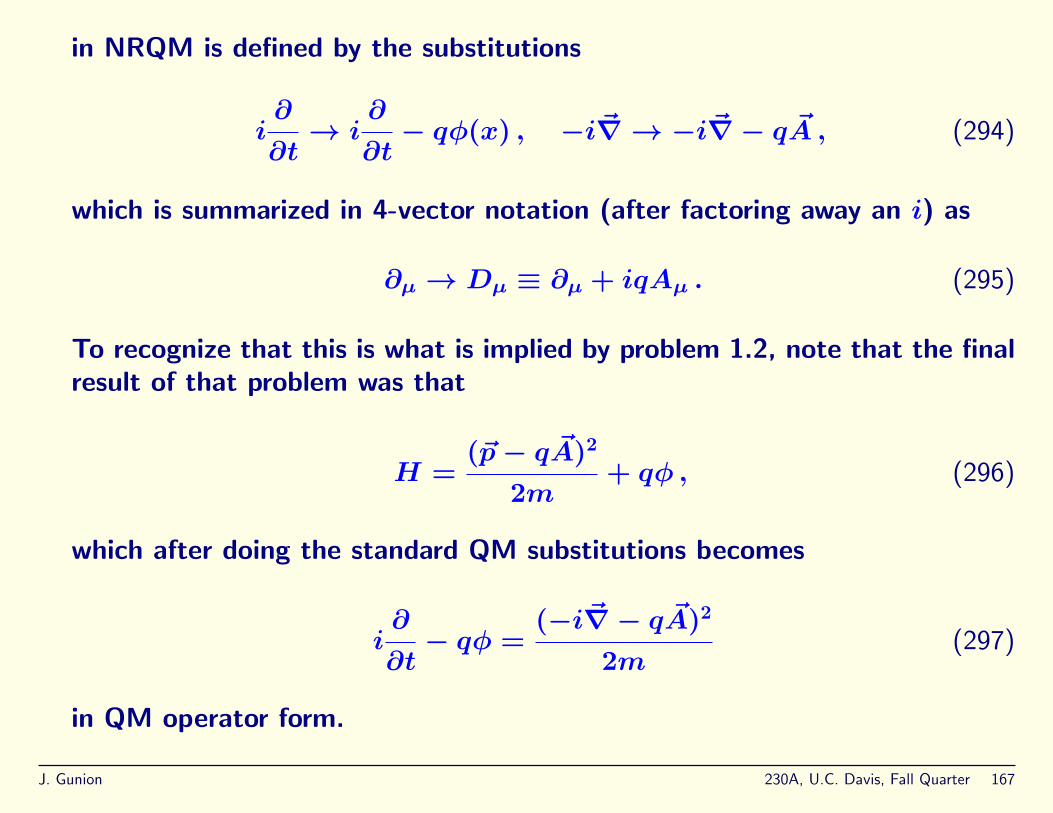
in NRQM is defined by the substitutions

i∂

∂t→ i

∂

∂t− qφ(x) , −i~∇ → −i~∇− q ~A , (294)

which is summarized in 4-vector notation (after factoring away an i) as

∂µ→ Dµ ≡ ∂µ + iqAµ . (295)

To recognize that this is what is implied by problem 1.2, note that the finalresult of that problem was that

H =(~p− q ~A)2

2m+ qφ , (296)

which after doing the standard QM substitutions becomes

i∂

∂t− qφ =

(−i~∇− q ~A)2

2m(297)

in QM operator form.


This clearly follows from the NRQM procedure and minimal substitutionrules asserted above as follows:

H =~p2

2m→ using QM operator substitutions

i∂

∂t=

(−i~∇)2

2m→ using minimal substitution rules

i∂

∂t− qφ =

(−i~∇− q ~A)2

2m. (298)

• If we follow this prescription in the Dirac Lagrangian, we get

L = ψ(x)(iD/ −m)ψ(x) = ψ(x)(i∂/ −m−qA/ )ψ(x) = LF +LI (299)

with (using q = −e for the electron)

LF = ψ(x)(i∂/−m)ψ(x) , LI = eψ(x)A/ ψ(x) = eψ(x)γµψ(x)Aµ(x) .(300)

LI is the interaction Lagrangian density.


• To obtain the complete Lagrangian density, we must add the Lagrangiandensity for the noninteracting Aµ field, LA = −1

4FµνFµν (plus some gauge

fixing stuff).

• The concept of an Elementary Particle

Now, the above interaction Lagrangian is not the only interaction Lagrangianthat can be written down. One could include, for example, an anomalousmagnetic moment interaction

∝ ψ(x)σµν

2mψ(x)Fµν (301)

which is gauge invariant (see ensuing discussion), Lorentz invariant and soforth. This type of interaction must be included when describing the wayin which a proton interacts with the Aµ field.

However, we know that the proton’s anomalous magnetic moment comesfrom the orbital motion of quarks around one another when the quarks aretreated as having only the interaction generated by the minimal substitutionrule.

Further, the proton is known to have a form factor that suppresses itsinteraction when probed by ~A at high momentum transfer. This is also


understood as being due to the composite nature of the proton, whereasthe quarks would not have such a form factor.

The minimal substitution rule implies that the fermion’s interactions withthe Aµ field are such that there is no anomalous magnetic moment (at“tree-level”, i.e. before we include loop “radiative” corrections) and noform factor.

This is our definition of what we mean by an elementary particle. Itis a particle whose interactions are generated entirely by the minimalsubstitution rule.

We are continuing to test the hypothesis that the leptons (the electron beingone of the leptons) and quarks are truly elementary in this sense. Every timewe build a new accelerator capable of higher momentum transfer probes, welook to see if the electron has a form factor that is not in agreement withthat computed using the interaction generated by the minimal substitutionrule to compute loop corrections to the tree-level prediction of no formfactor (i.e. F (q2) = 1, where F is the form factor and q is the momentumtransfer squared).

• Gauge invariance


1. We know that LA is invariant under Aµ→ Aµ + ∂µf(x).2. Under this substitution, we have

LI → LI + eψ(x)γµψ(x)∂µf(x) , (302)

which means a lack of gauge invariance.3. To compensate, we must introduce a transformation for ψ. The one that

works is a generalization of the “global” phase transformation related tocharge to a local phase transformation (i.e. x-dependent phase):

ψ(x)→ eief(x)ψ(x) , ψ(x)→ ψ(x)e−ief(x) (303)

This additional phase transformation does not affect LI (the phases ofψ and ψ just cancel one another), but because of the derivative in LFwe get

LF → LF − eψ(x)γµψ(x)∂µf(x) (304)

so that the change in LI is just compensated by the change in LF andL as a whole is unchanged by the local gauge transformation.

4. There is an intimate connection between local gauge invariance and aproperty of perturbative field theory called “renormalizability”. Basically,


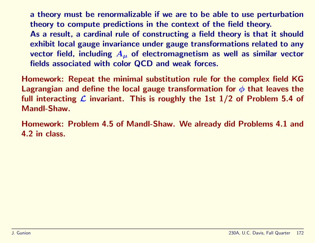
a theory must be renormalizable if we are to be able to use perturbationtheory to compute predictions in the context of the field theory.As a result, a cardinal rule of constructing a field theory is that it shouldexhibit local gauge invariance under gauge transformations related to anyvector field, including Aµ of electromagnetism as well as similar vectorfields associated with color QCD and weak forces.

Homework: Repeat the minimal substitution rule for the complex field KGLagrangian and define the local gauge transformation for φ that leaves thefull interacting L invariant. This is roughly the 1st 1/2 of Problem 5.4 ofMandl-Shaw.

Homework: Problem 4.5 of Mandl-Shaw. We already did Problems 4.1 and4.2 in class.


The Electromagnetic Field (again)

• The quantization procedure of Chapter 1 hides the Lorentz-invariance of thetheory — the decomposition of the fields into transverse and longitudinalcomponents is frame-dependent.

• We need an explicitly Lorentz-covariant formulation is order to prove thatwe can carry out calculations to arbitrary order in perturbation theory.

• We will employ the 4-vector potential Aµ(x) = (φ(x), ~A(x)).

However, it contains more degrees of freedom than the system actuallypossesses and the extra dof must be removed by imposing constraints.

• The formulation presented now is actually equivalent to the formulation ofChapter 1.

The Classical Fields


• We employFµν = ∂µAν(x)− ∂νAµ(x) , (305)

where µ labels the row and ν labels the column. This is opposite theMandl-Shaw convention (which is a terrible excursion from the norm); myconvention is the more usual convention. For example, see the book byRyder for correct conventions. I will be following Ryder’s notation in whatfollows. Sorry, but I don’t want you to get used to an uncommon conventionset.

Then, Fµν reduces to

Fµν =

0 −E1 −E2 −E3

E1 0 −B3 B2

E2 B3 0 −B1

E3 −B2 B1 0

(306)

To get the signs right in the above, we had to be very careful. For example,

F 01 = ∂0A1 − ∂1A0 = −(−∂

∂x0A1 − ~∇1φ) = −E1 (307)

where we used ∂1 = ∂∂x1

= − ∂∂x1 = −~∇1. More generally, Ei = −F 0i and


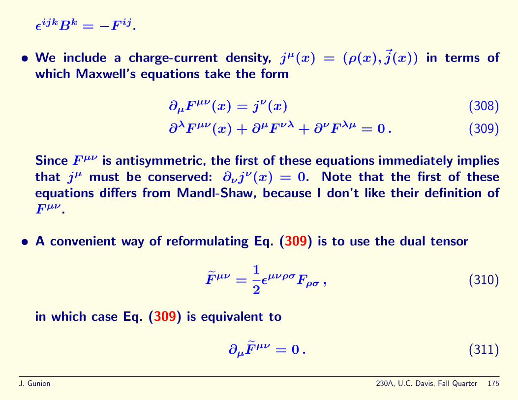
εijkBk = −F ij.

• We include a charge-current density, jµ(x) = (ρ(x),~j(x)) in terms ofwhich Maxwell’s equations take the form

∂µFµν(x) = jν(x) (308)

∂λFµν(x) + ∂µF νλ + ∂νFλµ = 0 . (309)

Since Fµν is antisymmetric, the first of these equations immediately impliesthat jµ must be conserved: ∂νj

ν(x) = 0. Note that the first of theseequations differs from Mandl-Shaw, because I don’t like their definition ofFµν.

• A convenient way of reformulating Eq. (309) is to use the dual tensor

Fµν =1

2εµνρσFρσ , (310)

in which case Eq. (309) is equivalent to

∂µFµν = 0 . (311)


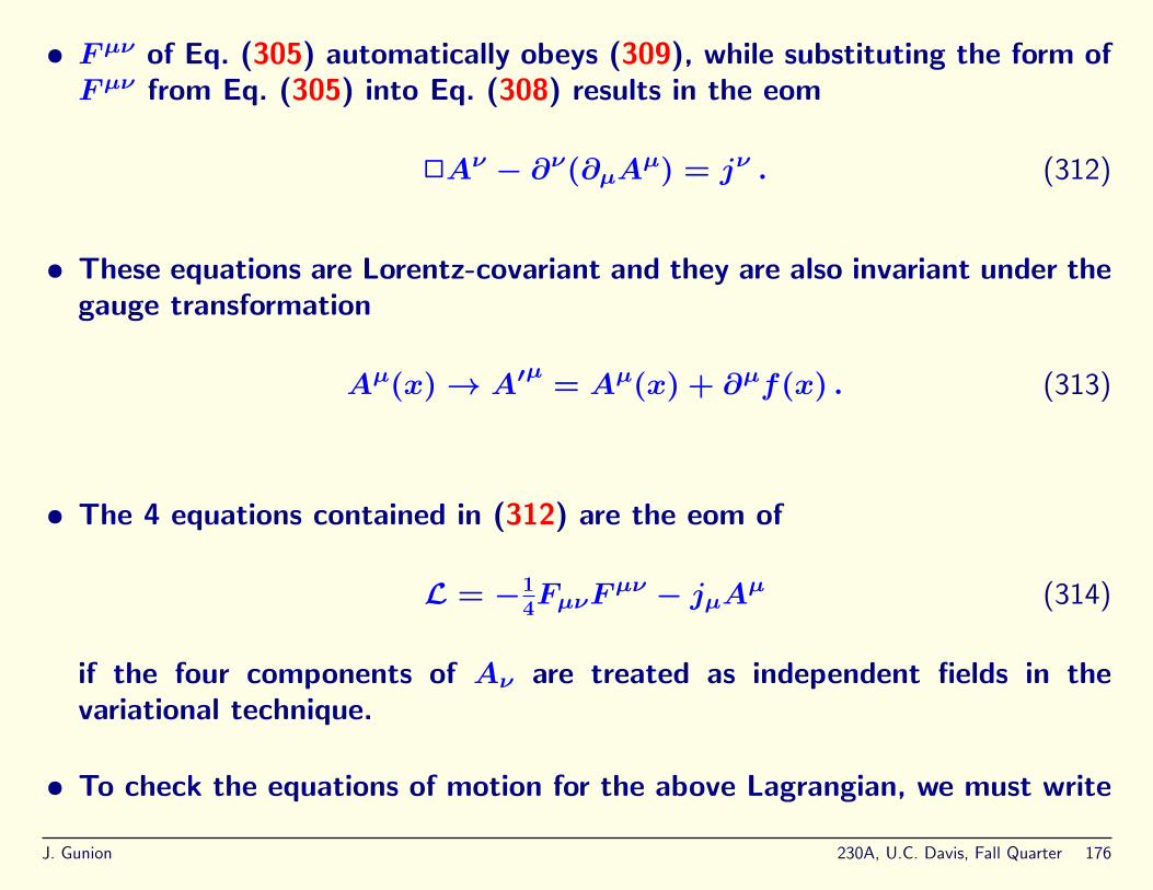
• Fµν of Eq. (305) automatically obeys (309), while substituting the form ofFµν from Eq. (305) into Eq. (308) results in the eom

2Aν − ∂ν(∂µAµ) = jν . (312)

• These equations are Lorentz-covariant and they are also invariant under thegauge transformation

Aµ(x)→ A′µ

= Aµ(x) + ∂µf(x) . (313)

• The 4 equations contained in (312) are the eom of

L = −14FµνF

µν − jµAµ (314)

if the four components of Aν are treated as independent fields in thevariational technique.

• To check the equations of motion for the above Lagrangian, we must write


out L in terms of the Aµ fields:

L = −14(∂ρAσ − ∂σAρ)gραgσβ(∂αAβ − ∂βAα)− jαAα , (315)

where we have been careful to use dummy summation indices in L. Now,think of dealing with each Aν component as the independent field.

∂L∂(∂µAν)

= −1

2(δµρδνσ − δµσδνρ)gραgσβ(∂αAβ − ∂βAα)

= −gµαgνβ(∂αAβ − ∂βAα)

= −(∂µAν − ∂νAµ) (316)

where, in the first equality we have used the fact that the α, β dummyindices would work just like the ρ, σ indices, thereby providing a factorof 2. The 2nd equality comes from using the α ↔ β antisymmetry of(∂αAβ − ∂βAα). We next compute

− ∂µ(

∂L∂(∂µAν)

)= 2Aν − ∂ν(∂µAµ) (317)


which is the LH side of Eq. (312). Meanwhile,

∂L∂Aν

= jν (318)

so that the eom becomes

0 = −∂µ(

∂L∂(∂µAν)

)+∂L∂Aν

= 2Aν − ∂ν(∂µAµ)− jν (319)

which is the desired result, Eq. (312), and obviously holds for each value ofν independently of every other value of ν.

• We note that L is clearly Lorentz invariant by construction. Further,although L is not gauge invariant, a gauge transformation does not affectthe equations of motion derived from L under certain provisos. To showthis and get the provisos, we note that Fµν is obviously gauge invariantwhile, under a gauge transformation,

jµAµ → jµA

µ + jµ∂µf


= jµAµ + ∂µ(jµf)− (∂µjµ)f

= jµAµ + ∂µ(jµf) (320)

by virtue of current conservation ∂µjµ = 0. The final form is equivalent tothe original L since this total 4-derivative can be added for free to L withoutchanging the equations of motion, provided that jµf only depends uponthe fields and not their derivatives. (This is problem 2.1 of Mandl-Shaw.)

Proof:

f must depend upon the fields in order for it to have any impact upon theequations of motion, so let us assume it has some arbitrary dependenceupon the fields Aν, but no dependence on the derivatives of the fields.jµ is assumed to depend upon other fields (so-called matter fields suchas electrons, quarks, ....). So, let us write the addition to L as δL =∂αΛα(Aβ). Then, we first note that

δL = ∂αΛα =∂Λα

∂Aβ∂αAβ (321)


by the chain rule. Then, the eom contribution from δL takes the form:

∂δL∂Aν

− ∂µ(

∂δL∂(∂µAν)

)= ∂α

(∂Λα

∂Aν

)− ∂µ

(∂Λα

∂Aβgµαgνβ

)= ∂α

(∂Λα

∂Aν

)− ∂µ

(∂Λµ

∂Aν

)= 0 (322)

In getting the form of the 2nd term on the LH side of the 1st equality, weused the explicit dependence of δL on ∂µAν written in Eq. (321). Thefinal cancellation just follows from dummy index relabeling.

Note that the cancellation between the two eom terms would fail if Λαdepended on the derivatives of the Aµ fields. For example, if it depended

only on the field derivatives, ∂δL∂Aν

= 0 while ∂µ(

∂δL∂(∂µAν)

)6= 0.

So, this implies that if we want to change the equation of motion (whichwe must in order to have an invertible kernel, i.e. a well-defined Green’sfunction/propagator) gauge fixing must involve derivatives of the Aµ(x)fields.


2nd quantization

• The conjugate fields are computed as

πν =∂L∂Aν

= −F 0ν (323)

where there are 4 terms contributing to the derivative, all of whichcontribute equally. This result implies that π0 = 0, and so impositionof canonical quantization conditions in the usual way is impossible for theA0 field.

• The other thing that goes wrong for the L = −14FµνF

µν Lagrangian formis the following.

One wants to be able to define the Feynman propagator as being the Greensfunction for the Kernel defined by the equation of motion in the absenceof any interactions. Recall that the equation of motion for the above L is(for the j = 0, free field, case)

2Aν − ∂ν(∂µAµ) = 0 (324)


which we rewrite as

(2gνµ − ∂ν∂µ)Aµ ≡ Kν

µAµ = 0 (325)

The K is the Kernel and the Greens function should obey

Kνα(x)Gαµ(x− y) = gνµδ

4(x− y) . (326)

Let us transform to momentum space. One then gets the equation

Kνα(k)Gαµ(k) = −(k2gνα − k

νkα)Gαµ(k) = gνµ . (327)

In other words G(k) should be basically the inverse of K(k).

I will now show that there is no solution to this equation, implying thatK does not have an inverse and that a Feynman propagator cannot bedefined. Let us suppose that there is a solution G(k). Lorentz covarianceimplies that the most general form it can take is

Gαµ(k) = a(k2)kαkµ + b(k2)gαµ . (328)


Plug this into Eq. (327) to obtain the consistency requirement

− k2b(k2)gνµ + b(k2)kνkµ = gνµ , (329)

to which there is no solution. (Note how the a(k2) stuff cancelled.)

This lack of an inverse is because K has many zero eigenvalues. AnyAµ ∝ ∂µf (i.e. a pure gauge transformation) obeys

Kνµ(x)∂µf(x) = 0 ! (330)

An operator with zero eigenvalues has no inverse.

Thus, we see that in order to get an invertible Kernel from our Lagrangianwe must specify a Lagrangian that has no zero eigenvalues, which inthe present context means that it should not be invariant under gaugetransformations — the Lagrangian should be that obtained after fixingsome particular gauge.

• An alternative form for L that does allow canonical procedures and does


generate an invertible equation of motion Kernel is

L = −1

2(∂µAν)(∂

µAν)− jµAµ . (331)

As we will see shortly, this L corresponds to having assumed the gauge-fixingcondition ∂µAµ = 0, called the Lorentz gauge.

For this L we find

πν =∂L∂Aν

= −Aν , (332)

which are all non-vanishing so that the canonical procedure can be appliedfor each Aν field independently.

• The eom for this alternative L are

2Aν(x) = jν(x) . (333)

• Is there a justification for making this change in L.

We note that (312) (2Aν − ∂ν(∂µAµ) = jν) reduces to (333) if we take

∂µAµ = 0 . (334)


This gauge condition must be imposed after the fact, i.e. after the 2ndquantization procedure based on L of (331), as a constraint or subsidiarycondition in order to maintain consistency with the original Maxwell equation(312).

• In the classical theory, starting from an arbitrary Aµ(x) we can alwaysfind a gauge transformation that gives ∂µA′µ = 0. We simply choose thefunction f in A′µ(x) = Aµ(x) + ∂µf(x) so that

∂µAµ(x) + 2f(x) = 0 (335)

which can be solved for f(x), but not uniquely since additional gaugetransformations obeying 2f = 0 would not further change ∂µAµ.

• The condition ∂µAµ = 0 is called the Lorentz gauge condition.

• The computational advantage of this choice over the previously discussed~∇ · ~A = 0 choice is that the eom are so much simpler. In particular, forjµ = 0, the eom reduce to

2Aν(x) = 0 , (336)


i.e. each Aν obeys a massless Klein-Gordon equation and we can 2ndquantize by taking over results from the KG discussion.

• We writeAν(x) = Aν+(x) +Aν−(x) (337)

with (assuming real polarization vectors, εr)

Aν+ =∑r~k

(1

2V ω~k

)1/2

ενr(~k)ar(~k)e−ik·x , (338)

Aν− =∑r~k

(1

2V ω~k

)1/2

ενr(~k)a†r(

~k)e+ik·x (339)

where k0 = ω~k = |~k| and r = 0, 1, 2, 3 to describe 4 fields. We choose theενr to be real and obey

εr(~k) · εs(~k) = −ζrδrs , r, s = 0, 1, 2, 3 ,∑r

ζrεµr (~k)ενr(

~k) = −gµν ,

(340)


where ζ0 = −1, ζ1,2,3 = +1. The two extra polarization states comparedto transverse (Coulomb) gauge provide a covariant description of theinstantaneous Coulomb interaction. A particularly convenient choice thatrealizes the above conditions is:

ε0(~k) = nµ ≡ (1, 0, 0, 0) (341)

εr(~k) = (0,~εr(~k)) , r = 1, 2, 3 (342)

~ε3(~k) =~k

|~k|(343)

~k · ~εr(~k) = 0 , r = 1, 2 (344)

~εr(~k) · ~εs(~k) = δrs, r, s = 1, 2, 3 . (345)

The ε1,2 are the transverse polarization vectors, ε3 is the longitudinalpolarization vector, and ε0 is referred to as the scalar or time-like polarizationvector.


For later use, we note that (using 4-vector notation)

ε3(~k) =k − (k · n)n

[(k · n)2 − k2]1/2. (346)

We have kept k2 6= 0 so that we can describe off-shell photons as well ason-shell photons using this set up.

Covariant 2nd Quantization

• We take jµ = 0 for the free-field case.

• We require

[Aµ(~x, t), Aν(~y, t)] = −igµνδ3(~x− ~y) (347)

and other commutators = 0. Note that covariance requires the gµν, so wemust learn how to deal with it. For µ = ν = j = 1, 2, 3, gµν = −1, andthe resulting −igjj = +i is exactly like the +i of the KG single field case.The implication and need for the −i for the µ = ν = 0 case will emergelater.


• Let us implement these conditions using KG or KG-like commutators forthe a, a† appearing in the “Fourier” decomposition written earlier. Inparticular, we will employ

[ar(~k), a†s(~p)] = ζrδrsδ~k~p (348)

with [a, a] and [a†, a†] commutators = 0. The fact that ζ0 = −1 appearsabove is required to get the “wrong”, i.e. negative, sign, i.e. −i, for theµ = ν = 0 field commutator of Eq. (347).

• Using the above, and following the KG procedures, we will obviously obtain

[Aµ(x), Aν(y)] = iDµν(x− y) , (349)

whereDµν(x) = −gµν∆(x,m = 0) . (350)

The Feynman propagator will similarly be given by

〈0|TAµ(x)Aν(y)|0〉 = iDµνF (x− y) (351)


where

DµνF (x) = −gµν∆F (x,m = 0) =

−gµν

(2π)4

∫d4k

e−ik·x

k2 + iε. (352)

• That the above is the correct result can be verified by simply checkingthat the Feynman propagator is indeed the Green’s function for theequation of motion, which for the Lagrangian we are employing, L =−1

2(∂µAν)(∂

µAν), means it should obey

2[iDµνF (x)] = −igµνδ4(x− y) (353)

which is obviously the case. Note that as above for µ = ν = i the signof the RHS is exactly what we had for a scalar field, whereas we have theopposite sign for µ = ν = 0 — this sign is required for a covariant formabove and elsewhere.

Gupta-Bleuler approach

• The basic steps are:


1. Interpret ar(~k) as absorption operators for all r = 0, 1, 2, 3.2. Interpret a†r(

~k) as creation operators for all r = 0, 1, 2, 3.

3. Define the vacuum state by ar(~k)|0〉 = 0 for all ~k and r = 0, 1, 2, 3.4. Define the 1-photon states by |1~kr〉 = a†r(

~k)|0〉.5. Compute

H =

∫d3~x : [πµAµ − L] : (354)

by substituting the expansions and using the properties of the εs’s ofEqs. (340)-(345) to obtain

H =∑s~p

ω~pζsa†s(~p)as(~p) . (355)

6. The “bad” sign for the s = 0 photons is actually ok since

H|1~kr〉 =∑~ps

ω~pζsa†s(~p)as(~p)a†r(

~k)|0〉 = +ω~ka†r(~k)|0〉, r = 0, 1, 2, 3

(356)is always positive. The extra ζrδrs in the commutators compensates theextra ζs in the H expression.


7. The number operators should be defined as

Nr(~k) = ζra†r(~k)ar(~k) (357)

for the same reason.

• But, there is a remaining problem. One finds states of negative norm:

〈1~kr|1~kr〉 = 〈0|ar(~k)a†r(~k)|0〉 = ζr〈0|0〉 = ζr (358)

which is −1 for r = 0. To eliminate this problem and to eliminate theextra r = 0, 3 non-transverse photon states, we must somehow bring backin the Lorentz gauge condition. We cannot do so as an operator identitybecause that would be incompatible with the commutation relations since

[∂µAµ(x), Aν(y)] = i∂µD

µν(x− y) 6= 0 (359)

for the form of Dµν obtained earlier as given in Eq. (350).

• The solution is to restrict the physical states by requiring

∂µAµ+(x)|Ψ〉 = 0 , (360)


which involves only absorption operators. The adjoint of this equation is

〈Ψ|∂µAµ−(x) = 0 . (361)

Then, for any state obeying this condition we have

〈Ψ|∂µAµ(x)|Ψ〉 = 〈Ψ|∂µAµ+(x) + ∂µAµ−(x)|Ψ〉 = 0 (362)

so that the Lorentz condition holds in the Quantum Mechanical expectationvalue sense for the allowed physical states. If we rewrite (360) in terms ofthe a operators, we find

[a3(~k)− a0(~k)]|Ψ〉 = 0 , for all ~k , (363)

and the adjoint

〈Ψ|[a†3(~k)− a†0(~k)] = 0 . (364)

These are constraints on the linear combinations of longitudinal and scalarphotons allowed in the state |Ψ〉. It places no constraint on the physicaltransverse photons present in a given state.


Derivation: We note that

∂µAµ+

=∑~k,r

1√2V |~k|

εµr (~k)ar(~k)∂µe

−ik·x

= −i∑~k,r

1√2V |~k|

kµεµr (~k)ar(~k)e

−ik·x

k·ε1,2=0= −i

∑~k,r=0,3

1√2V |~k|

kµεµr (~k)ar(~k)e

−ik·x

= −i∑~k

1√2V |~k|

e−ik·x

(k0ε

00(~k)a0(~k) + k0ε

03(~k)a3(~k)

−~k · ~ε0(~k)a0(~k)− ~k · ~ε3(~k)a3(~k))

= −i∑~k

1√2V |~k|

e−ik·x

(k0a0(~k) + 0a3(~k)− 0a0(~k)− ~k · ka3(~k)

)

= −i∑~k

1√2V |~k|

e−ik·x|~k|

(a0(~k)− a3(~k)

). (365)

In going from the 2nd to 3rd line, I used the fact that k · ε1,2 = 0 for thetransverse polarization states. The 4th line is obtained by simply writingthe 3rd line very explicitly. The 5th line is obtained by noting that ε0

0 = 1,

ε03 = 0, ~ε0 = 0 and ~ε3 = k. Since ∂µAµ

+|Ψ〉 = 0 for all x, and since each


~k gives a different spatial dependence, we must have Eq. (363).

• The result of this condition is apparent if we compute the vacuumexpectation value of the energy of an allowed state. From the formof H, this calculation will include

〈Ψ|a†3(~k)a3(~k)−a†0(~k)a0(~k)|Ψ〉 = 〈Ψ|a†3(~k)[a3(~k)−a0(~k)]|Ψ〉 = 0 (366)

where the first equality is obtained using the adjoint form of the constraint.Thus, we have

〈Ψ|H|Ψ〉 = 〈Ψ|∑~k

∑r=1,2

ω~ka†r(~k)ar(~k)|Ψ〉 (367)

so that only the transverse photons contribute to the expectation value ofthe energy. The same applies to other observables.

As far as negative norm states are concerned, it is not possible to have aphysical state defined by a†0(~k)|0〉 since

[a0(~k)− a3(~k)]a†0(~k)|0〉 = a0(~k)a†0(

~k)|0〉 = −|0〉 6= 0 . (368)


An allowed state would have to be a superposition state such as 1√2[a†0(

~k)−a†3(~k)]|0〉 which would obey the subsidiary condition as follows:

[a0(~k)− a3(~k)]1√

2[a†0(~k)− a†3(~k)]|0〉 =

1√

2[a0(~k)a

†0(~k) + a3(~k)a

†3(~k)]|0〉 =

1√

2[−1 + 1]|0〉 = 0 .

(369)

However, this kind of state is not actually a state at all. One way to seethis is that the norm of the above sample state is computed as:

1

2〈0|[a0(~k)−a3(~k)][a

†0(~k)−a†3(~k)]|0〉 =

1

2[a0(~k)a

†0(~k)+a3(~k)a

†3(~k)]|0〉 =

1

2[−1+1]|0〉 = 0 . (370)

In other words, adding in some allowed superposition of longitudinal andtime-like polarization states does not actually yield anything. You musthave some transverse stuff present in order to have a state with non-zeronorm. A typical state would be of the form that you will consider forProblem 5.3 of Mandl and Shaw:

|Ψ〉 =(1 + c[a†0(

~k)− a†3(~k)])|ΨT 〉 , (371)

where ΨT is a state containing some number of transversely polarizedphotons. From the computation of Eq. (370), it should be apparent that

〈Ψ|Ψ〉 = 〈ΨT |ΨT 〉 . (372)


• Although only the transverse photons matter for physical states, thepresence of the time-like and longitudinal photons is needed in a virtualsense when interactions mediated by the electromagnetic field enter thepicture.

Of the two extra (r = 0, 3) dof for each ~k, one is removed by the subsidiarystate condition (363) and the other corresponds to arbitrariness in thechoice of the Lorentz gauge (i.e. the specific way of implementing theLorentz condition). For instance, one can define the vacuum state |0〉 ascontaining no r = 0 or r = 3 states. This is the usual choice. So for theso-called “asymptotic states” where particles are not interacting, only thetransverse photons need to be kept.

But one could also define |0〉 as containing an appropriate mixture ofr = 0, 3 states so as to still satisfy Eq. (363). The many different suchpossibilities correspond to different Lorentz gauge choices, i.e. differentchoices of f obtained by shifting f → f + ∆f with 2∆f = 0.

Once a vacuum choice is made, one simply adds in the transverse photonsin the obvious way.

• Once we introduce charged matter fields, we can have virtual photon


propagation between charged fields. The propagator form will depend uponthe gauge choice.

However, so long as the initial and final “free-particle-like” states of aprocess obey the subsidiary conditions (i.e. are properly composed), at thevery end of the calculation the result will be independent of the gaugechosen.

• The better way to handle all of this is through path integrals. We willreturn to this in the section of notes labelled QFT-III.

The GB photon propagator interpretation

• Writing

DµνF =

1

(2π)4

∫d4kDµν

F (k)e−ik·x (373)

we have

DµνF (k) =

−gµν

k2 + iε=

1

k2 + iε

∑r

ζrεµr (~k)ενr(

~k) . (374)

• If we separate out the transverse part r = 1, 2 of this sum to define


TDµνF (k) then we can write

DµνF (k) =T D

µνF (k) +C D

µνF (k) +RD

µνF (k) (375)

where the first of the latter two guys corresponds to an instantaneousCoulomb potential interaction and the last “remainder” component can beshown to make no contribution to any physical process by virtue of currentconservation. Please read the Mandl-Shaw material on this.

In this way, we can understand that this covariant treatment is the same asthe Coulomb gauge treatment of Chapter 1, which also had real propagatingtransverse photons and an instantaneous Coulomb potential interaction (wedid not show this in lecture), and nothing more.

In any case, we shall employ the fully covariant form of DµνF in computing

scattering processes and such.

Problems 5.1 and 5.3 of Mandl-Shaw are assigned at this point.


Quantum Field Theory - University of California, Davishiggs.physics.ucdavis.edu/QFT-I.pdf · Class...

Documents

Transcript of Quantum Field Theory - University of California, Davishiggs.physics.ucdavis.edu/QFT-I.pdf · Class...