Quantum Field Theory II: Quantum Electrodynamics - Zeidler

Quantum Field Theory II: Quantum Electrodynamics

A Bridge between Mathematicians and Physicists

Bearbeitet vonEberhard Zeidler

2009 2008. Buch. xxxvii, 1101 S. HardcoverISBN 978 3 540 85376 3

Format (B x L): 15,5 x 23,5 cmGewicht: 1841 g

Weitere Fachgebiete > Physik, Astronomie > Elektrodynakmik, Optik > Elektrizität,Elektromagnetismus

Zu Inhaltsverzeichnis

schnell und portofrei erhältlich bei

Die Online-Fachbuchhandlung beck-shop.de ist spezialisiert auf Fachbücher, insbesondere Recht, Steuern und Wirtschaft.Im Sortiment finden Sie alle Medien (Bücher, Zeitschriften, CDs, eBooks, etc.) aller Verlage. Ergänzt wird das Programmdurch Services wie Neuerscheinungsdienst oder Zusammenstellungen von Büchern zu Sonderpreisen. Der Shop führt mehr

als 8 Millionen Produkte.

http://www.beck-shop.de/Zeidler-Quantum-Field-Theory-II-Quantum-Electrodynamics/productview.aspx?product=320681&utm_source=pdf&utm_medium=clickthru_lp&utm_campaign=pdf_320681&campaign=pdf/320681

http://www.beck-shop.de/trefferliste.aspx?toc=9344

http://www.beck-shop.de/trefferliste.aspx?toc=9344

http://www.beck-shop.de/fachbuch/inhaltsverzeichnis/9783540853763_TOC_001.pdf

1. Mathematical Principles of Modern NaturalPhilosophy

The book of nature is written in the language of mathematics.Galileo Galilei (1564–1642)

At the beginning of the seventeenth century, two great philosophers, Fran-cis Bacon (1561–1626) in England and Rene Descartes (1596–1650) inFrance, proclaimed the birth of modern science. Each of them describedhis vision of the future. Their visions were very different. Bacon said, “Alldepends on keeping the eye steadily fixed on the facts of nature.” Descartessaid, “I think, therefore I am.” According to Bacon, scientists should travelover the earth collecting facts, until the accumulated facts reveal how Na-ture works. The scientists will then induce from the facts the laws thatNature obeys. According to Descartes, scientists should stay at home anddeduce the laws of Nature by pure thought. In order to deduce the lawscorrectly, the scientists will need only the rules of logic and knowledge ofthe existence of God. For four hundred years since Bacon and Descartes ledthe way, science has raced ahead by following both paths simultaneously.Neither Baconian empiricism nor Cartesian dogmatism has the power toelucidate Nature’s secrets by itself, but both together have been amaz-ingly successful. For four hundred years English scientists have tended tobe Baconian and French scientists Cartesian.Faraday (1791–1867) and Darwin (1809–1882) and Rutherford (1871–1937) were Baconians; Pascal (1623–1662) and Laplace (1749–1827) andPoincare (1854–1912) were Cartesians. Science was greatly enriched by thecross-fertilization of the two contrasting national cultures. Both cultureswere always at work in both countries. Newton (1643–1727) was at hearta Cartesian, using pure thought as Descartes intended, and using it todemolish the Cartesian dogma of vortices. Marie Curie (1867–1934) wasat heart a Baconian, boiling tons of crude uranium ore to demolish thedogma of the indestructibility of atoms.1

Freeman Dyson, 2004

It is important for him who wants to discover not to confine himself to achapter of science, but keep in touch with various others.2

Jacques Hadamard (1865–1963)

1 From Dyson’s foreword to the book by P. Odifreddi, The Mathematical Century:The 30 Greatest Problems of the Last 100 Years, Princeton University Press,2004. Reprinted by permission of Princeton University Press.

2 J. Hadamard, The Psychology of Invention, Princeton University Press, 1945.

12 1. Mathematical Principles of Modern Natural Philosophy

Mathematics takes us still further from what is human, into the region ofabsolute necessity, to which not only the actual world, but every possibleworld must conform.3

Bertrand Russel (1872–1972)

1.1 Basic Principles

There exist the following fundamental principles for the mathematical de-scription of physical phenomena in nature.

(I) The infinitesimal principle due to Newton and Leibniz: The laws of naturebecome simple on an infinitesimal level of space and time.4

(II) The optimality principle (or the principle of least action): Physical pro-cesses proceed in such an optimal way that the action is minimal (or atleast critical). Such processes are governed by ordinary or partial differ-ential equations called the Euler–Lagrange equations.

(III) Emmy Noether’s symmetry principle: Symmetries of the action func-tional imply conservation laws for the corresponding Euler–Lagrangeequations (e.g., conservation of energy).

(IV) The gauge principle and Levi-Civita’s parallel transport: The funda-mental forces in nature (gravitational, eletromagnetic, strong, and weakinteraction) are based on the symmetry of the action functional un-der local gauge transformations. The corresponding parallel transportof physical information generates the intrinsic Gauss–Riemann–Cartan–Ehresmann curvature which, roughly speaking, corresponds to the actingforce (also called interaction). Briefly: force = curvature.

(V) Planck’s quantization principle: Nature jumps.(VI) Einstein’s principle of special relativity: Physics does not depend on the

choice of the inertial system.(VII) Einstein’s principle of general relativity: Physics does not depend on

the choice of the local space-time coordinates of an observer.(VIII) Dirac’s unitarity principle: Quantum physics does not depend on the

choice of the measurement device (i.e., on the choice of an orthonormalbasis in the relevant Hilbert space). This corresponds to the invarianceunder unitary transformations.5

3 The Earl of Russel was awarded the Nobel prize in literature in 1950. He workedin philosophy, mathematical logic, social sciences, and politics.

4 I. Newton, Philosophiae naturalis principia mathematica (Mathematical princi-ples of natural philosophy) (in Latin), 1687. Translated into English by A. Motte,in 1729, edited by F. Cajori, University of California Press, Berkeley, California,1946. See also S. Chandrasekhar, Newton’s Principia for the Common Reader,Oxford University Press, Oxford, 1997.

5 Newton (1643–1727), Leibniz (1646–1716), Euler (1707–1783), Lagrange (1736–1813), Laplace (1749–1828), Legendre (1752–1833), Fourier (1768–1830), Gauss(1777–1855), Poisson (1781–1840), Faraday (1791–1867), Green (1793–1841),

1.1 Basic Principles 13

Geometrization of physics. In mathematics, the properties of geomet-ric objects do not depend on the choice of the coordinate system. This issimilar to the principles (VI)–(VIII). Therefore, it is quite natural that geo-metric methods play a fundamental role in modern physics.

Linearity and nonlinearity. We have to distinguish between

(i) linear processes, and(ii) nonlinear processes.

In case (i), the superposition principle holds, that is, the superposition ofphysical states yields again a physical state. Mathematically, such processesare described by linear spaces and linear operator equations. The mathe-matical analysis can be simplified by representing physical phenomena assuperposition of simpler phenomena. This is the method of harmonic analy-sis (e.g., the Fourier method based on the Fourier series, the Fourier integral,or the Fourier–Stieltjes integral).

In case (ii), the superposition principle is violated. As a rule, interactionsin nature are mathematically described by nonlinear operator equations (e.g.,nonlinear differential or integral equations). The method of perturbation the-ory allows us to reduce (ii) to (i), by using an iterative method.

Basic properties of physical effects. For the mathematical investiga-tion of physical effects, one has to take the following into account.

(A) Faraday’s locality principle: Physical effects propagate locally in spaceand time (law of proximity theory).

(B) Green’s locality principle: The response of a linear physical system can bedescribed by localizing the external forces in space and time and by con-sidering the superposition of the corresponding special responses (methodof the Green’s function). Furthermore, this can be used for computingnonlinear physical systems by iteration.

(C) Planck’s constant: The smallest action (energy × time) in nature is givenby the action quantum h = 6.626 0755 · 10−34Js.

(D) Einstein’s propagation principle: Physical effects travel at most with thespeed of light c in a vacuum. Explicitly, c = 2.997 92458 · 108m/s.

(E) Gauge invariance principle: Physical effects are invariant under localgauge transformations. Physical experiments are only able to measurequantities which do not depend on the choice of the gauge condition.

Riemann (1826–1866), Maxwell (1831–1879), Lie (1842–1899), Klein (1849–

1925), Poincare (1854–1912), Planck (1858–1947), Elie Cartan (1859–1951),Hilbert (1862–1943), Minkowski (1864–1909), Levi-Civita (1873–1941), Einstein(1879–1955), Emmy Noether (1882–1935), Weyl (1885–1955), Schrodinger (1887–1961), Heisenberg (1901–1976), Dirac (1902–1984), Ehresmann (1905–1979),von Neumann (1903–1957), Tomonaga (1906–1979), Landau (1908–1968), Lau-rent Schwartz (1915–2002), Feynman (1918–1988), Schwinger (1918–1994), Yang(born 1922), Dyson (born 1923), Salam (1926–1996), Gell-Mann (born 1929),Glashow (born 1932), Weinberg (born 1933), Fritzsch (born 1943).


(F) The Planck scale hypothesis: Physics dramatically changes below thePlanck length given by l = 10−35m.

In what follows, let us discuss some basic ideas related to all of the principlessummarized above. To begin with, concerning Faraday’s locality principle,Maxwell emphasized the following:6

Before I began the study of electricity I resolved to read no mathematics onthe subject till I had first read through Faraday’s 1832 paper Experimentalresearches on electricity. I was aware that there was supposed to be adifference between Faraday’s way of conceiving phenomena and that ofthe mathematicians, so that neither he nor they were satisfied with eachother’s language. I had also the conviction that this discrepancy did notarise from either party being wrong. For instance, Faraday, in his mind, sawlines of force traversing all space where the mathematicians (e.g., Gauss)saw centers of force attracting at a distance; Faraday saw a medium wherethey saw nothing but distance; Faraday sought the seat of the phenomenain real actions going on in the medium, where they were satisfied that theyhad found it in a power of action at a distance impressed on the electricfluids.When I had translated what I considered to be Faraday’s ideas into amathematical form, I found that in general the results of the two methodscoincide. . . I also found that several of the most fertile methods of researchdiscovered by the mathematicians could be expressed much better in termsof the ideas derived from Faraday than in their original form.

1.2 The Infinitesimal Strategy and DifferentialEquations

Differential equations are the foundation of the natural scientific, mathe-matical view of the world.

Vladimir Igorevich Arnold (born 1937)

The infinitesimal strategy due to Newton and Leibniz studies the behavior ofa physical system for infinitesimally small time intervals and infinitesimallysmall distances. This leads to the encoding of physical processes into differen-tial equations (e.g., Newton’s equations of motion in mechanics, or Maxwell’sequations in electrodynamics).

The task of mathematics is to decode this information; that is, tosolve the fundamental differential equations.

1.3 The Optimality Principle

It is crucial that the class of possible differential equations is strongly re-stricted by the optimality principle. This principle tells us that the funda-mental differential equations are the Euler–Lagrange equations to variational6 J. Maxwell, A Treatise on Electricity and Magnetism, Oxford University Press,

Oxford, 1873.

1.4 The Basic Notion of Action in Physics and the Idea of Quantization 15

problems. In 1918, Emmy Noether formulated her general symmetry princi-ple in the calculus of variations. The famous Noether theorem combines Lie’stheory of continuous groups with the calculus of variations due to Euler andLagrange. This will be studied in Section 6.6.

1.4 The Basic Notion of Action in Physics and the Ideaof Quantization

The most important physical quantity in physics is not the energy, but theaction which has the physical dimension energy times time. The following iscrucial.

(i) The fundamental processes in nature are governed by the principle ofleast action

S = min!

where we have to add appropriate side conditions. In fact, one has to usethe more general principal S = critical! (principle of critical action). Forexample, if we consider the motion q = q(t) of a particle of mass m onthe real line, then the action is given by

S[q] :=∫ t1

t0

(12mq(t)2 − U(q(t))

)dt.

Here, the function U = U(q) is the potential, and the negative derivative,−U ′, describes the acting force. In this case, the principle of critical actionreads as

S[q] = critical!, q(t0) = q0, q(t1) = q1 (1.1)

where we fix the following quantities: the initial time t0, the initial posi-tion q0 of the particle, the final time t1, and the final position q1 of theparticle. The solutions of (1.1) satisfy the Euler–Lagrange equation

mq(t) = F (t), t ∈ R

with the force F (t) = −U ′(q(t)). This coincides with the Newtonianequation of motion (see Sect. 6.5).

(ii) In 1900 Planck postulated that there do not exist arbitrarily smallamounts of action in nature. The smallest amount of action in natureis equal to the Planck constant h. In ancient times, philosophers said:

Natura non facit saltus. (Nature does never make a jump.)In his “Noveaux essais,” Leibniz wrote:

Tout va par degres dans la nature et rien par saut. (In natureeverything proceeds little by little and not by jumping.)


In contrast to this classical philosophy, Planck formulated the hypothesisin 1900 that the energy levels of a harmonic oscillator form a discrete set.He used this fact in order to derive his radiation law for black bodies (seeSect. 2.3.1 of Vol. I). This was the birth of quantum physics. More gen-erally, the energy levels of the bound states of an atom or a molecule arediscrete. The corresponding energy jumps cause the spectra of atoms andmolecules observed in physical experiments (e.g., the spectral analysis ofthe light coming from stars). Nowadays, we say that:

Nature jumps.

This reflects a dramatic change in our philosophical understanding ofnature.

(iii) In order to mathematically describe quantum effects, one has to modifyclassical theories. This is called the process of quantization, which wewill encounter in this series of monographs again and again. As an in-troduction to this, we recommend reading Chapter 7. Now to the point.Feynman discovered in the early 1940s in his dissertation in Princetonthat the process of quantization can be most elegantly described by pathintegrals (also called functional integrals) of the form

∫eiS[ψ]/� Dψ

where we sum over all classical fields ψ (with appropriate side conditions).Here, � := h/2π. For example, the quantization of the classical particleconsidered in (i) can be based on the formula

G(q0, t0; q1, t1) =∫

eiS[q]/� Dq.

Here, we sum over all classical motions q = q(t) which satisfy the sidecondition q(t0) = q0 and q(t1) = q1. The Green’s function G determinesthe time-evolution of the wave function ψ, that is, if we know the wavefunction ψ = ψ(x, t0) at the initial time t0, then we know the wavefunction at the later time t by the formula

ψ(x, t) =∫

R

G(x, t; y, t0)ψ(y, t0)dy.

Finally, the wave function ψ tells us the probability

∫ b

a

|ψ(x, t)|2dx

of finding the quantum particle in the interval [a, b] at time t.

1.5 The Method of the Green’s Function 17

(iv) In quantum field theory, one uses the functional integral∫

eiS[ψ]/� ei〈ψ|J〉 Dψ

with the additional external source J . Differentiation with respect to Jyields the moments of the quantum field. In turn, the moments deter-mine the correlation functions (also called Green’s functions). The cor-relation functions describe the correlations between different positions ofthe quantum field at different points in time. These correlations are themost important properties of the quantum field which can be related tophysical measurements.

Feynman’s functional integral approach to quantum physics clearly showsthat both classical and quantum physics are governed by the classical actionfunctional S. This approach can also be extended to the study of many-particle systems at finite temperature, as we have discussed in Sect. 13.8 ofVol. I. Summarizing, let us formulate the following general strategy:

The main task in modern physics is the mathematical description ofthe propagation of physical effects caused by interactions and theirquantization.

In Sect. 1.9 we will show that in modern physics, interactions are describedby gauge theories based on local symmetries.

1.5 The Method of the Green’s Function

Basic ideas. As a prototype, consider the motion x = x(t) of a particleof mass m > 0 on the real line under the action of the continuous forceF : R → R. The corresponding Newtonian equation of motion reads as

mx(t) = F (t) for all t ∈ R (1.2)

with the initial condition

x(0) = a, x(0) = v.

We are given the initial position a and the initial velocity v at time t = 0.For simplifying notation, we set m := 1. In order to discuss Green’s localityprinciple in physics, let us summarize the following facts. The unique solutionof (1.2) reads as

x(t) = a + vt +∫ t

0

(t − τ)F (τ)dτ for all t ∈ R.

Equivalently, this can be written as


x(t) = a + vt +∫ ∞

−∞G(t, τ)F (τ)dτ for all t ∈ R. (1.3)

The function G is called the Green’s function of the differential equation(1.2). Explicitly,

G(t, τ) :=

⎧⎪⎨⎪⎩

t − τ if 0 ≤ τ ≤ t,

τ − t if t ≤ τ < 0,

0 otherwise.

Let us discuss the physical meaning of the Green’s function G. To this end,for fixed positive number Δt and all times t ∈ R, we introduce the DiracΔt-delta function

δΔt(t) :=

{1

Δt if 0 ≤ t ≤ Δt,

0 otherwise.

Obviously, we have

limΔt→+0

δΔt(t) =

{+∞ if 0 ≤ t ≤ Δt,

0 otherwise,

and the normalization condition∫ ∞−∞ δΔt(t)dt = 1 is satisfied.

(i) Localized force. We are given the parameters Δt > 0 and F0 ∈ R. Forfixed time t0, we choose the special force

F (t) := F0 · δΔt(t − t0) for all t ∈ R.

By (1.3), the corresponding motion reads as

xΔt(t) = a + vt + F0 ·1

Δt

∫ t0+Δt

t0

G(t, τ)dτ for all t ∈ R.

Letting Δt → +0, we get the motion7

x(t) = a + vt + F0 · G(t, t0) for all t ∈ R. (1.4)

This can be considered as the motion of the particle under the influenceof the kick force t �→ F0δΔt(t − t0) at time t0, as Δt → +0. For t0 ≥ 0,the motion (1.4) looks like

7 In fact, it follows from limε→+0 G(t, t0 + ε) = G(t, t0) for all t, t0 ∈ R that

limΔ→+0

1

Δt

Z t0+Δt

t0

G(t, τ)dτ = G(t, t0).

1.5 The Method of the Green’s Function 19

x(t) =

{a + vt if t < t0,

a + vt + F0 · (t − t0) if t ≥ t0.(1.5)

That is, the velocity jumps at time t0. For t0 < 0, (1.4) looks like

x(t) =

{a + vt if t > t0,

a + vt + F0 · (t0 − t) if t ≤ t0.(1.6)

(ii) Superposition of the original force by kick forces (physical interpretationof the Green’s function). Fix Δt > 0. Consider the discrete points in timenΔt where n = 0,±1,±2, . . . In terms of physics, let us approximate thegiven force F = F (t) by a step function Fapprox. That is, we use thesuperposition

Fapprox(t) :=∞∑

n=−∞Fn(t), t ∈ R

of the kick forces Fn(t) := F (nΔt)δΔt(t − nΔt)Δt. Explicitly,

Fn(t) =

{F (nΔt) if nΔt ≤ t ≤ (n + 1)Δt,

0 otherwise.

If Δt is sufficiently small, then the kick force Fn generates the approxi-mate motion

xn(t) = F (nΔt)G(t, nΔt)Δt, t ∈ R

with xn(0) = 0 and xn(0) = 0 for all n = ±1,±2, . . . That is, the particlerests at the initial time t = 0. Consequently, by superposition, the forceFapprox generates the approximate motion

xapprox(t) =∞∑

n=−∞xn(t) =

∞∑n=−∞

G(t, nΔt)F (nΔt)Δt, t ∈ R.

As Δt → 0, we get the motion x(t) =∫ ∞−∞ G(t, τ)F (τ)dτ for all t ∈ R.

The motions (1.5) and (1.6) have the following properties:

(a) t �→ x(t) is continuous on R.(b) t �→ x(t) is smooth on R \ {t0}, and x(t) = 0 for all t �= t0.(c) x(t0 + 0) = x(t0 − 0) + F0 (jump of the velocity at time t0).(d) In the sense of distributions, we have the following equation of motion:8

mx(t) = F0δ(t − t0), t ∈ R.

8 We choose m := 1.


Let us prove (d). We have to show that∫ ∞

−∞x(t)ϕ(t)dt = F0ϕ(t0) for all ϕ ∈ D(R).

Noting (b), integration by parts yields that∫ ∞

t0x(t)ϕ(t)dt is equal to

−x(t0)ϕ(t0) −∫ ∞

t0

x(t)ϕ(t)dt = −x(t0)ϕ(t0) + x(t0 + 0)ϕ(t0).

Similarly,∫ t0−∞ x(t)ϕ(t)dt = x(t0)ϕ(t0) − x(t0 − 0)ϕ(t0). Finally, use (c). �

Examples. Fix t0 := 0 and F0 := 1. If we choose a = v := 0, then themotion (1.5) looks like

x(t) = θ(t)t for all t ∈ R.

Here, θ denotes the Heaviside function.9 If we choose a := 0 and v := −1,then the motion (1.5) looks like

x(t) = −θ(−t)t for all t ∈ R.

Finally, if we choose a := 0, v := −12 , then the motion (1.5) looks like

x(t) = 12 (θ(t)t − θ(−t)t) = 1

2 |t| for all t ∈ R.

The relation between the theory of distributions and the method of averagingwill be discussed in Sect. 1.7.

Iterative solution of nonlinear problems. The experience of physi-cists shows that

Interactions in nature lead to nonlinear terms in the correspondingdifferential equations.

This explains the importance of nonlinear problems in physics. We wantto show that the Green’s function can also be used in order to investigatenonlinear problems. As a prototype, consider the differential equation

mx(t) = −κx(t)3, t ∈ R (1.7)

with the positive parameter κ called coupling constant, and the initial con-dition x(0) = a, x(0) = v. This problem describes an anharmonic oscillator(see page 370). By (1.3), the initial-value problem (1.7) is equivalent to thenonlinear integral equation

x(t) = a + vt − κ

∫ ∞

−∞G(t, τ)x(τ)3dτ for all t ∈ R, (1.8)

9 Recall that θ(t) := 1 if t ≥ 0 and θ(t) := 0 if t < 0.

1.6 Harmonic Analysis and the Fourier Method 21

by setting F (t) := −κx(t)3. The corresponding iterative method reads as

xn+1(t) = a + vt − κ

∫ ∞

−∞G(t, τ)xn(τ)3dτ, n = −1, 0, 1, . . .

with x−1(t) := 0 for all t ∈ R. This iterative method is also called thebootstrap method by physicists. In particular, x0(t) = a + vt for all t ∈ R.The first approximation,

x1(t) = a + vt − κ

∫ ∞

−∞G(t, τ)x0(τ)3dτ for all t ∈ R

is called the Born approximation by physicists. If the coupling constant κ issufficiently small, then the iterative method converges to the solution of theoriginal integral equation (1.8), that is, limn→∞ xn(t) = x(t) for all t ∈ R.

The two problems (1.7) and (1.8) reflect a crucial duality between dif-ferential equations and integral equations. The kernel G of the inte-gral equation (1.8) is the Green’s function of the linearized differentialequation (1.2).

In this series of monographs, we will frequently use this duality. For example,in Sect. 8.6 we will study stationary scattering processes in quantum mechan-ics by replacing the Schrodinger differential equation by the dual Lippmann–Schwinger integral equation.

Therefore, nonlinear problems can be iteratively solved if the Green’sfunction is known.

This is the method of perturbation theory, which is basic for quantum fieldtheory. For the computation of the Green’s function, one can use Fourier’smethod. For the Newtonian motion (1.2), this will be studied in Sect. 2.2.14in terms of the Fourier integral transform.

1.6 Harmonic Analysis and the Fourier Method

The superposition principle. In 1822 Fourier published his monographTheorie analytique de la chaleur (analytic heat theory) where he used boththe Fourier series and the Fourier integral in order to solve numerous problemsin heat conduction. Let us sketch the basic ideas. For given time period T > 0,let us introduce the corresponding angular frequency

Δω :=2π

T.

Fourier’s method of harmonic analysis is the most important method for get-ting explicit solutions of linear partial differential equations in mathematicalphysics and for explicitly computing the corresponding Green’s functions.10

10 Much material can be found in P. Morse and H. Feshbach, Methods of TheoreticalPhysics, Vols. 1, 2, McGraw-Hill, New York, 1953. Fourier’s method is intimately


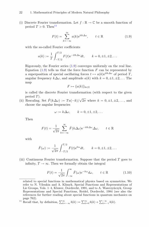
(i) Discrete Fourier transformation. Let f : R → C be a smooth function ofperiod T > 0. Then11

F (t) =∞∑

k=−∞a(k)eitkΔω, t ∈ R (1.9)

with the so-called Fourier coefficients

a(k) :=1T

∫ T/2

−T/2

F (t)e−itkΔωdt, k = 0,±1,±2, . . .

Rigorously, the Fourier series (1.9) converges uniformly on the real line.Equation (1.9) tells us that the force function F can be represented bya superposition of special oscillating forces t �→ a(k)eitkΔω of period T ,angular frequency kΔω, and amplitude a(k) with k = 0,±1,±2, . . . Themap

F �→ {a(k)}k∈Z

is called the discrete Fourier transformation (with respect to the givenperiod T ).

(ii) Rescaling. Set F (kΔω) := Ta(−k)/√

2π where k = 0,±1,±2, . . . , andchoose the angular frequencies

ω := kΔω, k = 0,±1,±2, . . .

Then

F (t) =1√2π

∞∑k=−∞

F (kΔω)e−itkΔωΔω, t ∈ R

with

F (ω) :=1√2π

∫ T/2

−T/2

F (t)eitωdt, k = 0,±1,±2, . . .

(iii) Continuous Fourier transformation. Suppose that the period T goes toinfinity, T → ∞. Then we formally obtain the integral

F (t) =1√2π

∫ ∞

−∞F (ω)e−itωdω, t ∈ R (1.10)

related to special functions in mathematical physics based on symmetries. Werefer to N. Vilenkin and A. Klimyk, Special Functions and Representations ofLie Groups, Vols. 1–4, Kluwer, Dordrecht, 1991, and to A. Wawrzynczyk, GroupRepresentations and Special Functions, Reidel, Dordrecht, 1984 (see also thereferences for further reading about special functions in quantum mechanics onpage 762).

11 Recall that, by definition,P∞

k=−∞ b(k) :=P∞

k=0 b(k) +P−∞

k=−1 b(k).


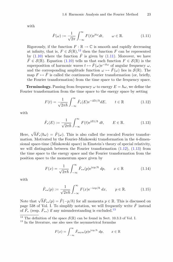
with

F (ω) :=1√2π

∫ ∞

−∞F (t)eitωdt, ω ∈ R. (1.11)

Rigorously, if the function F : R → C is smooth and rapidly decreasingat infinity, that is, F ∈ S(R),12 then the function F can be representedby (1.10) where the function F is given by (1.11). Moreover, we haveF ∈ S(R). Equation (1.10) tells us that each function F ∈ S(R) is thesuperposition of harmonic waves t �→ F (ω)e−itω of angular frequency ω,and the corresponding amplitude function ω �→ F (ω) lies in S(R). Themap F �→ F is called the continuous Fourier transformation (or, briefly,the Fourier transformation) from the time space to the frequency space.

Terminology. Passing from frequency ω to energy E = �ω, we define theFourier transformation from the time space to the energy space by setting

F (t) =1√2π�

∫ ∞

−∞F∗(E)e−iEt/�dE, t ∈ R (1.12)

with

F∗(E) :=1√2π�

∫ ∞

−∞F (t)eiEt/� dt, E ∈ R. (1.13)

Here,√

�F∗(�ω) = F (ω). This is also called the rescaled Fourier transfor-mation. Motivated by the Fourier-Minkowski transformation in the 4-dimen-sional space-time (Minkowski space) in Einstein’s theory of special relativity,we will distinguish between the Fourier transformation (1.12), (1.13) fromthe time space to the energy space and the Fourier transformation from theposition space to the momentum space given by

F (x) =1√2π�

∫ ∞

−∞F∗∗(p)eixp/� dp, x ∈ R (1.14)

with

F∗∗(p) :=1√2π�

∫ ∞

−∞F (x)e−ixp/� dx, p ∈ R. (1.15)

Note that√

�F∗∗(p) = F (−p/�) for all momenta p ∈ R. This is discussed onpage 538 of Vol. I. To simplify notation, we will frequently write F insteadof F∗ (resp. F∗∗) if any misunderstanding is excluded.13

12 The definition of the space S(R) can be found in Sect. 10.3.3 of Vol. I.13 In the literature, one also uses the asymmetrical formulas

F (x) =

Z ∞

−∞Fasym(p)eixp/� dp, x ∈ R


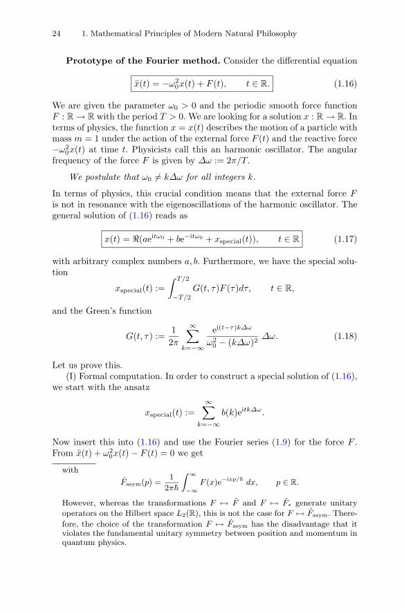
Prototype of the Fourier method. Consider the differential equation

x(t) = −ω20x(t) + F (t), t ∈ R. (1.16)

We are given the parameter ω0 > 0 and the periodic smooth force functionF : R → R with the period T > 0. We are looking for a solution x : R → R. Interms of physics, the function x = x(t) describes the motion of a particle withmass m = 1 under the action of the external force F (t) and the reactive force−ω2

0x(t) at time t. Physicists call this an harmonic oscillator. The angularfrequency of the force F is given by Δω := 2π/T.

We postulate that ω0 �= kΔω for all integers k.

In terms of physics, this crucial condition means that the external force Fis not in resonance with the eigenoscillations of the harmonic oscillator. Thegeneral solution of (1.16) reads as

x(t) = (aeitω0 + be−itω0 + xspecial(t)), t ∈ R (1.17)

with arbitrary complex numbers a, b. Furthermore, we have the special solu-tion

xspecial(t) :=∫ T/2

−T/2

G(t, τ)F (τ)dτ, t ∈ R,

and the Green’s function

G(t, τ) :=12π

∞∑k=−∞

ei(t−τ)kΔω

ω20 − (kΔω)2

Δω. (1.18)

Let us prove this.(I) Formal computation. In order to construct a special solution of (1.16),

we start with the ansatz

xspecial(t) :=∞∑

k=−∞b(k)eitkΔω.

Now insert this into (1.16) and use the Fourier series (1.9) for the force F .From x(t) + ω2

0x(t) − F (t) = 0 we get

with

Fasym(p) =1

2π�

Z ∞

−∞F (x)e−ixp/� dx, p ∈ R.

However, whereas the transformations F �→ F and F �→ F∗ generate unitary

operators on the Hilbert space L2(R), this is not the case for F �→ Fasym. There-

fore, the choice of the transformation F �→ Fasym has the disadvantage that itviolates the fundamental unitary symmetry between position and momentum inquantum physics.


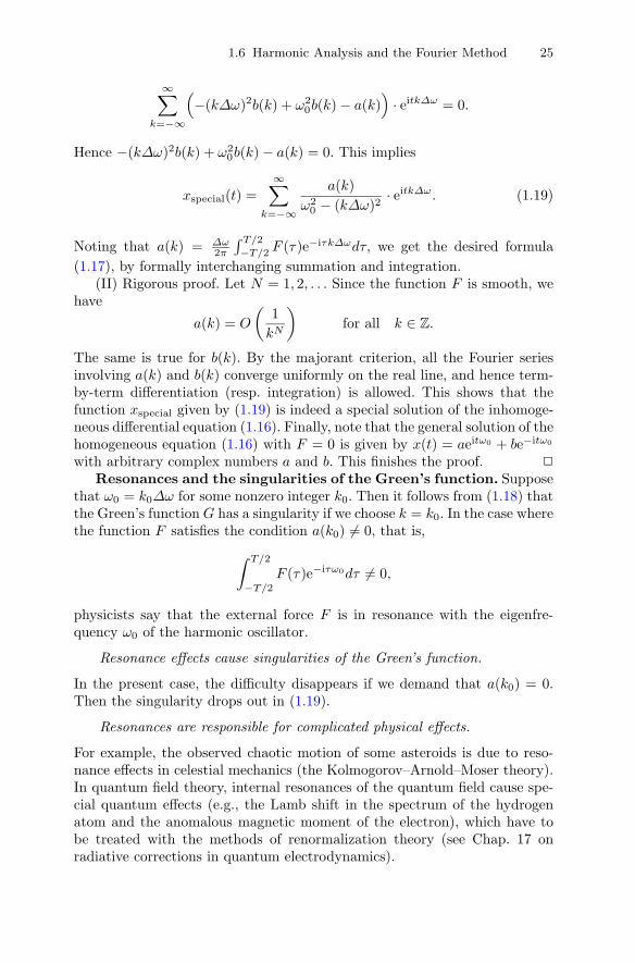
∞∑k=−∞

(−(kΔω)2b(k) + ω2

0b(k) − a(k))· eitkΔω = 0.

Hence −(kΔω)2b(k) + ω20b(k) − a(k) = 0. This implies

xspecial(t) =∞∑

k=−∞

a(k)ω2

0 − (kΔω)2· eitkΔω. (1.19)

Noting that a(k) = Δω2π

∫ T/2

−T/2F (τ)e−iτkΔωdτ, we get the desired formula

(1.17), by formally interchanging summation and integration.(II) Rigorous proof. Let N = 1, 2, . . . Since the function F is smooth, we

have

a(k) = O

(1

kN

)for all k ∈ Z.

The same is true for b(k). By the majorant criterion, all the Fourier seriesinvolving a(k) and b(k) converge uniformly on the real line, and hence term-by-term differentiation (resp. integration) is allowed. This shows that thefunction xspecial given by (1.19) is indeed a special solution of the inhomoge-neous differential equation (1.16). Finally, note that the general solution of thehomogeneous equation (1.16) with F = 0 is given by x(t) = aeitω0 + be−itω0

with arbitrary complex numbers a and b. This finishes the proof. �

Resonances and the singularities of the Green’s function. Supposethat ω0 = k0Δω for some nonzero integer k0. Then it follows from (1.18) thatthe Green’s function G has a singularity if we choose k = k0. In the case wherethe function F satisfies the condition a(k0) �= 0, that is,

∫ T/2

−T/2

F (τ)e−iτω0dτ �= 0,

physicists say that the external force F is in resonance with the eigenfre-quency ω0 of the harmonic oscillator.

Resonance effects cause singularities of the Green’s function.

In the present case, the difficulty disappears if we demand that a(k0) = 0.Then the singularity drops out in (1.19).

Resonances are responsible for complicated physical effects.

For example, the observed chaotic motion of some asteroids is due to reso-nance effects in celestial mechanics (the Kolmogorov–Arnold–Moser theory).In quantum field theory, internal resonances of the quantum field cause spe-cial quantum effects (e.g., the Lamb shift in the spectrum of the hydrogenatom and the anomalous magnetic moment of the electron), which have tobe treated with the methods of renormalization theory (see Chap. 17 onradiative corrections in quantum electrodynamics).


1.7 The Method of Averaging and the Theory ofDistributions

In the early 20th century, mathematicians and physicists noticed that forwave problems, the Green’s functions possess strong singularities such thatthe solution formulas of the type (1.3) fail to exist as classical integrals.14 Inhis classic monograph

The Principles of Quantum Mechanics,

Clarendon Press, Oxford, 1930, Dirac introduced a singular object δ(t) (theDirac delta function), which is very useful for the description of quantumprocesses and the computation of Green’s functions. In the 1940s, LaurentSchwartz gave all these approaches a sound basis by introducing the notionof distribution (generalized function). In order to explain Laurent Schwartz’sbasic idea of averaging, consider the continuous motion

x(t) := |t| for all t ∈ R

of a particle on the real line. We want to compute the force F (t) = mx(t)acting on the particle at time t. Classically, F (t) = 0 if t �= 0, and the forcedoes not exist at the point in time t = 0. We want to motivate that

F (t) = 2mδ(t) for all t ∈ R. (1.20)

(I) The language of Dirac. For the velocity, x(t) = 1 if t > 0, and x(t) = −1if t < 0. For t = 0, the derivative x(0) does not exist. We define x(0) := 0.Hence

x(t) = θ(t) − θ(−t).

Since θ(t) = δ(t), we get

x(t) = δ(t) + δ(−t) = 2δ(t) for all t ∈ R.

Formally, δ(t) = 0 if t �= 0, and δ(0) = ∞ with∫ ∞−∞ δ(t)dt = 1. Obviously,

there is no classical function δ which has such properties.15

(II) The language of Laurent Schwartz. Choose ε > 0. We first pass to theregularized motion x = xε(t) for all t ∈ R. That is, the function xε : R → R

is smooth for all ε > 0 and14 For example, see J. Hadamard, The Initial-Value Problem for Linear Hyperbolic

Partial Differential Equations, Hermann, Paris (in French). A modern versionof Hadamard’s theory can be found in P. Gunther, Huygens’ Principle and Hy-perbolic Differential Equations, Academic Press, San Diego, 1988. See also C.Bar, N. Ginoux, and F. Pfaffle, Wave Equations on Lorentzian Manifolds andQuantization, European Mathematical Society 2007.

15 See the detailed discussion of the formal Dirac calculus in Sect. 11.2 of Vol. I.

1.7 The Method of Averaging and the Theory of Distributions 27

limε→+0

xε(t) = |t| for all t ∈ R,

where this convergence is uniform on all compact time intervals.16 We intro-duce the averaged force

Fε(ϕ) :=∫ ∞

−∞mxε(t)ϕ(t)dt

for all averaging functions ϕ ∈ D(R) (i.e., ϕ : R → C is smooth and vanishesoutside some bounded interval. In other words, ϕ has compact support.) Sincexε is smooth, integration by parts twice yields

Fε(ϕ) =∫ ∞

−∞mxε(t)ϕ(t)dt.

Letting ε → +0, we define the mean force by

F(ϕ) := limε→+0

Fε(ϕ) =∫ ∞

−∞mx(t)ϕ(t)dt.

Integration by parts yields∫ ∞0

|t| ϕ(t)dt = −∫ ∞0

ϕ(t)dt = ϕ(0). Similarly,∫ 0

−∞ |t|ϕ(t)dt = −∫ 0

−∞ ϕ(t)dt = ϕ(0). Summarizing, we obtain the averagedforce

F(ϕ) = 2mϕ(0) for all ϕ ∈ D(R). (1.21)

In the language of distributions, we have F = 2mδ, where δ denotes theDirac delta distribution. A detailed study of the theory of distributions andits applications to physics can be found in Chaps. 11 and 12 of Vol. I. Inparticular, equation (1.20) is equivalent to (1.21), in the sense of distributiontheory.

In terms of experimental physics, distributions correspond to the factthat measurement devices only measure averaged values. It turns out thatclassical functions can also be regarded as distributions. However, in contrastto classical functions, the following is true:

Distributions possess derivatives of all orders.

Therefore, the theory of distributions is the quite natural completion of theinfinitesimal strategy due to Newton and Leibniz, who lived almost threehundred years before Laurent Schwartz. This shows convincingly that thedevelopment of mathematics needs time.16 For example, choose xε(t) := rε(t)|t| for all t ∈ R, where the regularizing function

rε : R → [0, 1] is smooth, and rε(t) := 1 if t /∈ [−2ε, 2ε], as well as rε(t) := 0 ift ∈ [−ε, ε].


1.8 The Symbolic Method

The symbol of the operator ddt . Consider again the Fourier transforma-

tion

F (t) =1√2π

∫ ∞

−∞F (ω)e−itωdω, t ∈ R (1.22)

with

F (ω) :=1√2π

∫ ∞

−∞F (t)eitωtdt, ω ∈ R. (1.23)

Let n = 1, 2, . . . Differentiation of (1.22) yields

dn

dtnF (t) =

1√2π

∫ ∞

−∞(−iω)nF (ω)eitωdω, t ∈ R. (1.24)

The functions(ω) := −iω for all ω ∈ R

is called the symbol of the differential operator ddt . For n = 0, 1, 2, . . . , we

havedn

dtnF ⇒ snF .

This means that the action of the differential operator dn

dtn , with respect totime t, can be described by the multiplication of the Fourier transform F bysn in the frequency space.

This corresponds to a convenient algebraization of derivatives.

Over the centuries, mathematicians and physicists tried to simplify compu-tations. The relation

ln(ab) = ln a + ln b for all a, b > 0 (1.25)

allows us to reduce multiplication to addition. This fact was extensively usedby Kepler (1571–1630) in order to simplify his enormous computations incelestial mechanics.

Similarly, the Fourier transformation allows us to reduce differenti-ation to multiplication.

Furthermore, there exists a natural generalization of the logarithmic functionto Lie groups. Then the crucial formula (1.25) passes over to the transforma-tion formula from the Lie group G to its Lie algebra LG. This transformationis well defined for the group elements near the unit element (see Vol. III).

Pseudo-differential operators and Fourier integral operators. Themodern theory of pseudo-differential operators (e.g., differential and integral

1.8 The Symbolic Method 29

operators) and Fourier integral operators is based on the use of symbols ofthe form

s = s(ω, t, τ),

which depend on frequency ω, time t, and time τ . The expressions

(AF )(t) :=12π

∫R2

s(ω, t, τ)F (τ)eiω(τ−t) dτdω, t ∈ R (1.26)

and

(BF )(t) :=12π

∫R2

s(ω, t, τ)F (τ)eiϕ(ω,t,τ) dτdω, t ∈ R (1.27)

correspond to the pseudo-differential operator A and the Fourier integraloperator B. If we choose the special phase function

ϕ(ω, t, τ) := ω(t − τ),

then the operator B passes over to A. If, in addition, the symbol s does notdepend on τ , then integration over τ yields

(AF )(t) =1√2π

∫ ∞

−∞s(ω, t)F (ω)e−iωt dω.

In the special case where the symbol s(ω, t) only depends on the frequencyω, the pseudo-differential operator corresponds to the multiplication operatorω �→ s(ω)F (ω) in the frequency space (also called Fourier space).

Long before the foundation of the theory of pseudo-differential operatorsand Fourier integral operators in the 1960s and 1970s, mathematicians andphysicists used integral expressions of the form (1.26) and (1.27) in order tocompute explicit solutions in electrodynamics (e.g., the Heaviside calculusand the Laplace transform applied to the study of electric circuits17), elastic-ity (singular integral equations), geometric optics (e.g., diffraction of light),and quantum mechanics.

The point is that the symbols know a lot about the properties of thecorresponding operators, and an elegant algebraic calculus for opera-tors can be based on algebraic operations for the symbols.

As an introduction, we recommend:

Yu. Egorov and M. Shubin, Foundations of the Classical Theory of PartialDifferential Equations, Springer, New York, 1998 (Encyclopedia of Math-ematical Sciences).

Yu. Egorov, A. Komech, and M. Shubin, Elements of the Modern Theoryof Partial Differential Equations, Springer, New York, 1999 (Encyclopediaof Mathematical Sciences).

17 See E. Zeidler (Ed.), Oxford Users’ Guide to Mathematics, Sect. 1.11, OxfordUniversity Press, 2004.


F. Berezin and M. Shubin, The Schrodinger Equation, Kluwer, Dordrecht,1991.

L. Faddeev and A. Slavnov, Gauge Fields, Benjamin, Reading, Mas-sachusetts, 1980 (gauge theory, Weyl calculus, the Feynman path integral,and the Faddeev–Popov ghost approach to the Standard Model in particlephysics).

We also refer to the following treatises:

L. Hormander, The Analysis of Linear Partial Differential Operators.Vol. 1: Distribution Theory and Fourier Analysis, Vol. 2: Differential Op-erators with Constant Coefficients, Vol. 3: Pseudo-Differential Operators,Vol. 4: Fourier Integral Operators, Springer, New York, 1993.

R. Dautray and J. Lions, Mathematical Analysis and Numerical Methodsfor Science and Technology, Vols. 1–6, Springer, New York, 1988.

Heaviside’s formal approach. Consider the differential equation

d

dtx(t) − x(t) = f(t). (1.28)

We want to discuss the beauty, but also the shortcomings of the symbolicmethod due to Heaviside (1850–1925). Formally, we get

(d

dt− 1

)x(t) = f(t).

Hence

x(t) =f(t)ddt − 1

.

For complex numbers z with |z| < 1, we have the convergent geometric series1

z−1 = −1 − z − z2 − z3 + ... This motivates

x(t) =(−1 − d

dt− d2

dt2− . . .

)f(t). (1.29)

If we choose f(t) := t2, then

x(t) = −t2 − 2t − 2. (1.30)

Surprisingly enough, we get x(t) = −2t−2 = x(t)+t2. Therefore, the functionx(t) from (1.30) is a solution of (1.28). The same is true for all polynomials.To prove this, let f be a polynomial of degree n = 0, 1, 2 . . . Set

x(t) := −n∑

k=0

dk

dtkf(t).

Then we get x(t) = −∑n

k=0dk+1

dtk+1 f(t) = f(t) + x(t), since the (n + 1)thderivative of f vanishes. However, the method above fails if we apply it tothe exponential function f(t) := et. Then


x(t) = et + et + et + . . . ,

which is meaningless. There arises the problem of establishing a more pow-erful method. In the history of mathematics and physics, formal (also calledsymbolic) methods were rigorously justified by using the following tools:

• the Fourier transformation,• the Laplace transformation (which can be reduced to the Fourier transfor-

mation),• Mikusinski’s operational calculus based on the quotient field over a convo-

lution algebra,• von Neumann’s operator calculus in Hilbert space,• the theory of distributions,• pseudo-differential operators and distributions (e.g., the Weyl calculus in

quantum mechanics), and• Fourier integral operators and distributions.

Mikusinski’s elegant approach will be considered in Sect. 4.2 on page 191.Motivation of the Laplace transformation via Fourier transfor-

mation. Consider the motion x = x(t) of a particle on the real line withx(t) = 0 for all t ≤ 0. Suppose that the function x : R → R is continuousand bounded. The Fourier transform from the time space to the energy spacereads as

x(E) =1√2π�

∫ ∞

−∞x(t)eiEt/� dt =

1√2π�

∫ ∞

0

x(t)eiEt/� dt.

As a rule, this integral does not exist. To improve the situation, we fix theregularization parameter ε > 0, and we define the damped motion

xε(t) := x(t)e−εt for all t ∈ R.

This is also called the adiabatic regularization of the original motion. Obvi-ously, limε→+0 xε(t) = x(t) for all t ∈ R. The Fourier transform looks like

xε(E) =1√2π�

∫ ∞

0

x(t)e−εteiEt/� dt =1√2π�

∫ ∞

0

x(t)eiEt/� dt,

by introducing the complex energy E := E + iε. To simplify notation, we set� := 1.

Complex energies, damped oscillations, and the Laplace trans-form. The formal Heaviside calculus was justified by Doetsch in the 1930s byusing the Laplace transform.18 As a simple example, let us use the Laplacetransformation in order to solve the differential equation (1.28). In particular,we will consider the case18 G. Doetsch, Theory and Applications of the Laplace Transform, Springer, Berlin,

1937 (in German). See also D. Widder, The Laplace Transform, Princeton Uni-versity Press, 1944.


f(t) := et

where the Heaviside method above fails. Let x : [0,∞[→ R be a smoothfunction with the growth condition

|x(t)| ≤ const · eγ1t for all t ≥ 0

and fixed real number γ1. The Laplace transform reads as

L(x)(E) :=∫ ∞

0

x(t) eiEt dt, �(E) > γ1 (1.31)

with the inverse transform

x(t) =12π

PV

∫L

(Lx)(E)e−iEtdE , t > 0 (1.32)

on the real line L := {E + (γ1 + 1)i : E ∈ R} of the complex energy space.Here, we choose a system of units with � = h/2π := 1 for Planck’s actionquantum.19 The Laplace transform sends the function t �→ x(t) on the timespace to the function E �→ (Lx)(E) on the complex energy space. Here, it iscrucial to use complex energies E = E − Γ i. In what follows, we will use thestandard properties of the Laplace transformation which are proved in Sect.2.2.6 of Vol. I. Let us start with an example. Choose the complex energyE0 := E0 − Γ0i with real values E0 and Γ0, and set20

x(t) := e−iE0t = e−iE0t · e−Γ0t, t ∈ R. (1.33)

Then, γ1 = −Γ0 = �(E0), and we get

(Lx)(E) =i

E − E0, �(E) > �(E0).

Now to the point. We are given the smooth function f : [0,∞[→ C with thegrowth condition

|f(t)| ≤ const · eγ0t for all t ≥ 0.

In order to solve the differential equation (1.28), we proceed as follows.(I) Suppose first that the differential equation (1.28) has a smooth solution

x : [0,∞[→ C with |x(t)| ≤ const · eγ1t for all t ≥ 0 with γ1 ≥ γ0. Then19 Set γ2 := γ1 + 1. The principal value of the integral is defined by

PV

Z

L

g(E)dE := limE0→+∞

Z E0+γ2i

−E0+γ2i

g(E + γ2i)dE.

20 If E0 > 0 and Γ0 > 0 then (1.33) is a damped oscillation with angular frequencyω0 := E0/� = E0 and mean lifetime Δt = Γ0/� = Γ0.


the Laplace transforms Lx and Lf exist for all E ∈ C with �(E) > γ1.Furthermore,

(Lx)(E) = −iE(L)(E) − x(+0),

that is, the Laplace transforms converts differentiation into multiplicationand translation in the complex energy space. By (1.28),

−iE(Lx)(E) − (Lx)(E) − x(+0) = (Lf)(E), �(E) > γ1.

This yields the Laplace transform of the solution t → x(t), namely,

(Lx)(E) =ix(+0)E − i

+i(Lf)(E)E − i

.

Setting g(t) := et, we get (Lg)(E) = iE−i . Therefore,

Lx = (Lg)x(+0) + (Lg)(Lf).

The convolution rule from Sect. 2.2.6 of Vol. I tells us that

x = gx(+0) + g ∗ f.

Explicitly, this reads as

x(t) = etx(+0) +∫ t

0

e(t−τ)f(τ)dτ. (1.34)

Our argument shows that a solution of (1.28) has necessarily the form (1.34).(II) Conversely, differentiation yields

x(t) = etx(+0) + f(t) +∫ t

0

e(t−τ)f(τ)dτ = x(t) + f(t)

for all t ≥ 0. Consequently, the function x = x(t) given by (1.34) is indeeda solution of the original differential equation (1.28) for all times t ≥ 0. Forexample, if f(t) := et, then

x(t) = etx(+0) + tet.

This is a solution of (1.28) for all times t ∈ R.The same method of the Laplace transformation can be applied to general

systems of ordinary differential equations with constant coefficients. Suchequations are basic for the investigation of electrical circuits. Therefore, theLaplace transformation plays a key role in electrical engineering.

34 1. Mathematical Principles of Natural Philosophy

1.9 Gauge Theory – Local Symmetry and theDescription of Interactions by Gauge Fields

As we have discussed in Chap. 2 of Vol. I, the Standard Model in particlephysics is based on

• 12 basic particles (6 quarks and 6 leptons), and• 12 interacting particles (the photon, the 3 vector bosons W+, W−, Z0 and

8 gluons).

This model was formulated in the 1960s and early 1970s. Note the followingcrucial fact about the structure of the fundamental interactions in nature.

The fields of the interacting particles can be obtained from the fieldsof the basic particles by using the principle of local symmetry (alsocalled the gauge principle).

Prototype of a gauge theory. Let us explain the basic ideas by consid-ering the following simple model. To this end, let us choose the unit squareQ := {(x, t) : 0 ≤ x, t ≤ 1}. We start with the principle of critical action

∫Q

L(ψ, ψt, ψx; ψ†, ψ†t , ψ

†x) dxdt = critical! (1.35)

with the boundary condition ψ = ψ0 on ∂Q and the special Lagrangian

L := ψ†ψt + ψ†ψx. (1.36)

Here, ψt (resp. ψx) denotes the partial derivative of ψ with respect to timet (resp. position x). We are given a fixed continuous function ψ0 : ∂Q → C

on the boundary of the square Q. We are looking for a smooth functionψ : Q → C which solves the variational problem (1.35).

By a basic result from the calculus of variations, we get the following.If the function ψ is a solution of (1.35), then it is a solution of the twoEuler–Lagrange equations

∂

∂tLψ†

t+

∂

∂xLψ†

x= Lψ† (1.37)

and

∂

∂tLψt +

∂

∂xLψx = Lψ. (1.38)

Here, the symbol Lψ (resp. Lψ†) denotes the partial derivative of L withrespect to the variable ψ (resp. ψ†). The proof can be found in Problem 14.7of Vol. I. Explicitly, the two Euler–Lagrange equations read as

ψt + ψx = 0, ψ†t + ψ†

x = 0. (1.39)

1.9 Gauge Theory and Local Symmetry 35

If the function ψ is a solution of (1.39), then we have

(ψψ†)t + (ψψ†)x = 0, (1.40)

which is called a conservation law. In fact, ψtψ† + ψ†

t ψ = −ψxψ† − ψ†xψ.

This is equal to −(ψψ†)x. Conservation laws play a fundamental role in allfields of physics, since they simplify the computation of solutions. In the 18thand 19th century, astronomers unsuccessfully tried to find 6N conservationlaws for the motion of N bodies in celestial mechanics (N ≥ 3), in order tocompute the solution and to prove the stability of our solar system.21

Step by step, mathematicians and physicists discovered that

Conservation laws are intimately related to symmetries.

The precise formulation of this principle is the content of the Noether theoremproved in 1918 (see Sect. 6.6). We want to show that the invariance of theLagrangian L (with respect to a global gauge transformation) is behind theconservation law (1.40).

(i) Global symmetry and the Noether theorem. Let α be a fixed real number.We consider the global symmetry transformation

ψ+(x, t) := eiαψ(x, t) for all x, t ∈ R, (1.41)

that is, the field ψ is multiplied by the constant phase factor eiα, whereα is called the phase. The transformation (1.41) is also called a globalgauge transformation, by physicists. We also define the infinitesimalgauge transformation δψ by setting

δψ(x, t) :=d

dα

(eiαψ(x, t)

)|α=0

= iψ(x, t).

This means that ψ+(x, t) = 1+α ·δψ(x, t)+O(α2) as α → 0. Noting thatψ†

+ = e−iαψ†, the special Lagrangian L from (1.36) is invariant under theglobal gauge transformation (1.41), that is,

ψ†+(ψ+)t + ψ†

+(ψ+)x = ψ†ψt + ψ†ψx.

Generally, the Lagrangian L is invariant under the global gauge trans-formation (1.41) iff

L(ψ+, (ψ+)t, (ψ+)x; ψ†+, (ψ†

+)t, (ψ†+)x) = L(ψ, ψt, ψx; ψ†, ψ†

t , ψ†x).

21 See D. Boccaletti and G. Pucacco, Theory of Orbits, Vol 1: Integrable Systemsand Non-Perturbative Methods, Vol. 2: Perturbative and Geometrical Methods,Springer, Berlin, 1996.Y. Hagihara, Celestial Mechanics, Vols. 1–5, MIT Press, Cambridge, Mas-sachusetts, 1976.W. Neutsch and K. Scherer, Celestial Mechanics: An Introduction to Classicaland Contemporary Methods, Wissenschaftsverlag, Mannheim, 1992.


Then a special case of the famous Noether theorem on page 387 tells usthe following: If the function ψ is a solution of the variational problem(1.35), then

∂

∂t

(Lψtδψ + Lψ†

tδψ†

)+

∂

∂x

(Lψxδψ + Lψ†

xδψ†

)= 0.

If we choose the special Lagrangian L = ψ†ψt + ψ†ψx, then we obtainthe conservation law (1.40).

(ii) Local symmetry and the covariant derivative. We now replace the globalgauge transformation (1.40) by the following local gauge transformation

ψ+(x, t) := eiα(x,t)ψ(x, t) for all x, t ∈ R, (1.42)

where the phase α depends on space and time. We postulate the followingcrucial local symmetry principle:

(P) The Lagrangian L is invariant under local gauge transforma-tions.

It can be easily shown that the function L from (1.36) does not possessthis invariance property for arbitrary functions α = α(x, t). This followsfrom

(ψ+)t = iαteiαψ + eiαψt.

Here, the appearance of the derivative αt of the phase function α destroysthe invariance property of L.Our goal is to modify the function L in such a way that it is invariantunder (1.42). To this end, we introduce the so-called covariant partialderivatives

∇t :=∂

∂t+ iU(x, t), ∇x :=

∂

∂x+ iA(x, t), (1.43)

where U, A : R2 → R are given smooth real-valued functions called gauge

fields. The local gauge transformation of U and A is defined by

U+ := U − αt, A+ := A − αx.

Furthermore, we define the following transformation law for the covariantpartial derivatives:

∇+t :=

∂

∂t+ iU+, ∇+

x :=∂

∂x+ iA+. (1.44)

The key relation is given by the following elegant transformation law forthe covariant partial derivatives:

∇+t ψ+ = eiα∇tψ, ∇+

x ψ+ = eiα∇xψ. (1.45)


Theorem 1.1 There holds (1.45).

This theorem tells us the crucial fact that, in contrast to the classicalpartial derivatives, the covariant partial derivatives are transformed inthe same way as the field ψ itself. This property is typical for covariantpartial derivatives in mathematics. Indeed, our construction of covariantpartial derivatives has been chosen in such a way that (1.45) is valid.Proof. By the product rule,

(∂

∂t+ iU+

)ψ+ = eiα(iαtψ + ψt + iU+ψ) = eiα

(∂

∂t+ iU

)ψ.

This yields ∇+t ψ+ = eiα∇tψ. Similarly, we get ∇+

x ψ+ = eiα∇xψ. �

Now let us discuss the main idea of gauge theory:

We replace the classical partial derivatives ∂∂t ,

∂∂x by the covariant

partial derivatives ∇t,∇x, respectively.

This is the main trick of gauge theory. In particular, we replace theLagrangian

L = ψ† ∂

∂tψ + ψ† ∂

∂xψ

from the original variational problem (1.35) by the modified Lagrangian

L := ψ†∇tψ + ψ†∇xψ.

Explicitly, we have

L = ψ†ψt + ψ†ψx + iψ†Uψ + iψ†Aψ.

The corresponding Euler–Lagrange equations (1.37) and (1.38) read as

∇tψ + ∇xψ = 0, (1.46)

and (∇tψ + ∇xψ)† = 0, respectively.

The local symmetry principle (P) above is closely related to the Faraday–Green locality principle, saying that physical interactions are localized inspace and time.

Summarizing, the local symmetry principle (P) enforces the existenceof additional gauge fields U, A which interact with the originally givenfield ψ.

In the Standard Model in particle physics and in the theory of general rela-tivity, the additional gauge fields are responsible for the interacting particles.

Consequently, the mathematical structure of the fundamental inter-actions in nature is a consequence of the local symmetry principle.


In his search of a unified theory for all interactions in nature, Einstein wasnot successful, since he was not aware of the importance of the principle oflocal symmetry. In our discussion below, the following notions will be crucial:

• local gauge transformation,• gauge force F ,• connection form A,• curvature form F (gauge force form), and• parallel transport of information.

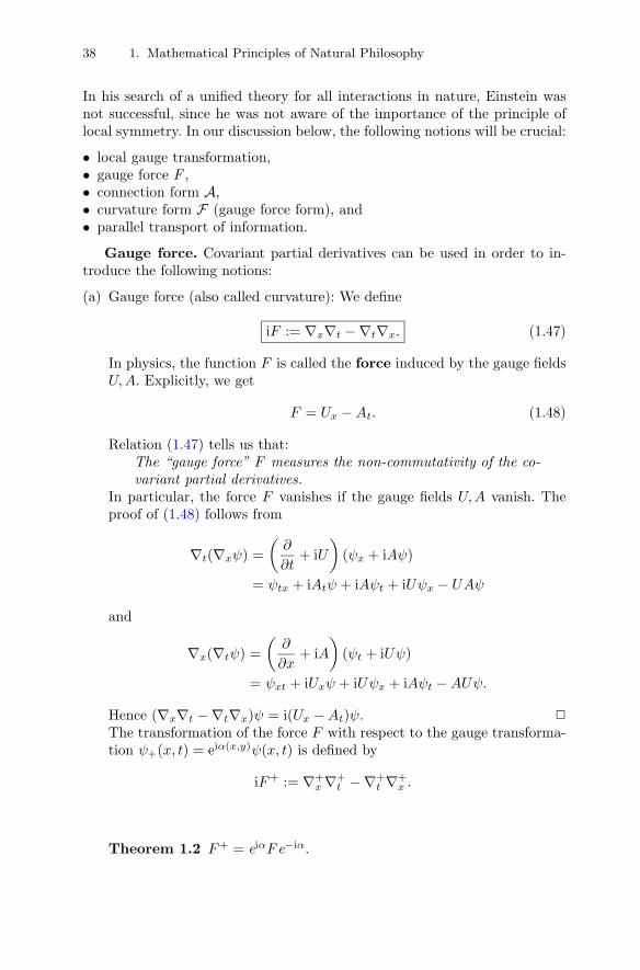
Gauge force. Covariant partial derivatives can be used in order to in-troduce the following notions:

(a) Gauge force (also called curvature): We define

iF := ∇x∇t −∇t∇x. (1.47)

In physics, the function F is called the force induced by the gauge fieldsU, A. Explicitly, we get

F = Ux − At. (1.48)

Relation (1.47) tells us that:The “gauge force” F measures the non-commutativity of the co-variant partial derivatives.

In particular, the force F vanishes if the gauge fields U, A vanish. Theproof of (1.48) follows from

∇t(∇xψ) =(

∂

∂t+ iU

)(ψx + iAψ)

= ψtx + iAtψ + iAψt + iUψx − UAψ

and

∇x(∇tψ) =(

∂

∂x+ iA

)(ψt + iUψ)

= ψxt + iUxψ + iUψx + iAψt − AUψ.

Hence (∇x∇t −∇t∇x)ψ = i(Ux − At)ψ. �

The transformation of the force F with respect to the gauge transforma-tion ψ+(x, t) = eiα(x,y)ψ(x, t) is defined by

iF+ := ∇+x ∇+

t −∇+t ∇+

x .

Theorem 1.2 F+ = eiαF e−iα.


Proof. It follows from Theorem 1.1 on page 37 that

iF+ψ+ = (∇+x ∇+

t −∇+t ∇+

x )ψ+ = ∇+x (eiα∇tψ) −∇+

t (eiα∇xψ)= eiα(∇x∇tψ −∇t∇xψ) = eiαiFψ = (eiαiF e−iα)ψ+.

�

In the present case, we have the commutativity property F e−iα = e−iαF.Hence

F+ = eiαe−iαF = F,

that is, the force F is gauge invariant. In more general gauge theories,the phase factor eiα(x,t) is a matrix. In this case, the force F is not gaugeinvariant anymore. However, it is possible to construct gauge invariantswhich depend on F . This is the case for the Standard Model in particlephysics (see Vol. III).

(b) Covariant directional derivative: Consider the curve

C : x = x(σ), t = t(σ),

where the curve parameter σ varies in the interval [0, σ0]. The classicaldirectional derivative along the curve C is defined by

d

dσ:=

dx(σ)dσ

∂

∂x+

dt(σ)dσ

∂

∂t.

Explicitly, we get

d

dσψ(x(σ), t(σ)) =

dx(σ)dσ

ψx(x(σ), t(σ)) +dt(σ)dσ

ψt(x(σ), t(σ)).

Similarly, the covariant directional derivative along the curve C is definedby

D

dσ:=

dx(σ)dσ

∇x +dt(σ)dσ

∇t.

Explicitly,

D

dσψ(x(σ), t(σ)) =

d

dσψ(x(σ), t(σ)) + iA(x(σ)), t(σ))

dx(σ)dσ

+iU(x(σ), t(σ))dt(σ)dσ

. (1.49)

(c) Parallel transport: We say that the field function ψ is parallel along thecurve C iff

D

dσψ(x(σ), t(σ)) = 0, 0 ≤ σ ≤ σ0. (1.50)

By (1.49), this notion depends on the gauge fields U, A. In particular, ifthe gauge fields U, A vanish, then parallel transport means that the fieldψ is constant along the curve C.


The following observation is crucial. It follows from the key relation (1.45)on page 36 that the equation (1.50) of parallel transport is invariant underlocal gauge transformations. This means that (1.50) implies

D+

dσψ+(x(σ), t(σ)) = 0, 0 ≤ σ ≤ σ0.

Consequently, in terms of mathematics, parallel transport possesses a geo-metric meaning with respect to local symmetry transformations.

In terms of physics, parallel transport describes the transport of phys-ical information in space and time.

This transport is local in space and time, which reflects the Faraday–Greenlocality principle.

The Cartan differential. The most elegant formulation of gauge theo-ries is based on the use of the covariant Cartan differential. As a preparation,let us recall the classical Cartan calculus. We will use the following relations:

dx ∧ dt = −dt ∧ dx, dx ∧ dx = 0, dt ∧ dt = 0. (1.51)

Moreover, the wedge product of three factors of the form dx, dt is alwaysequal to zero. For example,

dx ∧ dt ∧ dt = 0, dt ∧ dx ∧ dt = 0. (1.52)

For the wedge product, both the distributive law and the associative law arevalid. Let ψ : R

2 → C be a smooth function. By definition,

• dψ := ψxdx + ψtdt.

The differential 1-form

A := iAdx + iUdt (1.53)

is called the Cartan connection form. By definition,

• dA := idA ∧ dx + idU ∧ dt,• d(ψ dx ∧ dt) = dψ ∧ dx ∧ dt = 0 (Poincare identity).

The Poincare identity is a consequence of (1.52).The covariant Cartan differential. We now replace the classical par-

tial derivatives by the corresponding covariant partial derivatives. Therefore,we replace dψ by the definition

• Dψ := ∇xψ dx + ∇tψ dt.

Similarly, we define

• DA := iDA ∧ dx + iDU ∧ dt,• D(ψ dx ∧ dt) = Dψ ∧ dx ∧ dt = 0 (Bianchi identity).


The Bianchi identity is a consequence of (1.52). Let us introduce the Cartancurvature form F by setting

F := DA. (1.54)

Theorem 1.3 (i) Dψ = dψ + Aψ.(ii) F = dA + A ∧A (Cartan’s structural equation).(iii) DF = 0 (Bianchi identity).

In addition, we have the following relations for the curvature form F :

• F = dA + [U, A]−.22

• F = iFdx ∧ dt, where iF = Ux − At.

Proof. Ad (i). Dψ = (ψx + iAψ)dx + (ψt + iUψ)dt.Ad (ii). Note that

DA = i(Ax + A2)dx + i(At + iUA)dt,

DU = i(Ux + iAU)dx + (Ut + iU2)dt,

and

A ∧A = −(Adx + Udt) ∧ (Adx + Udt) = (UA − AU) dx ∧ dt.

Hence

DA = iDA ∧ dx + iDU ∧ dt

= i(At + iUA) dt ∧ dx + i(Ux + iAU) dx ∧ dt = dA + A ∧A.

This yields all the identities claimed above. �

The results concerning the curvature form F above show that Cartan’sstructural equation (1.54) is nothing else than a reformulation of the equation

iF = Ux − At,

which relates the force F to the potentials U, A. Furthermore, we will showin Sect. 5.11 on page 333 that Cartan’s structural equation is closely relatedto both

• Gauss’ theorema egregium on the computation of the Gaussian curvature ofa classic surfaces by means of the metric tensor and its partial derivatives,

• and the Riemann formula for the computation of the Riemann curvaturetensor of a Riemannian manifold by means of the metric tensor and itspartial derivatives.

In the present case, the formulas can be simplified in the following way. Itfollows from the commutativity property AU = UA that:22 Here, we use the Lie bracket [U, A]− := UA − AU.


• F = dA,• F = iF dx ∧ dt = i(Ux − At) dx ∧ dt.

A similar situation appears in Maxwell’s theory of electromagnetism. Formore general gauge theories, the symbols A and U represent matrices. Thenwe obtain the additional nonzero terms [U, A]− and A ∧ A. This is the casein the Standard Model of elementary particles (see Vol. III).

The mathematical language of fiber bundles. In mathematics, weproceed as follows:

• We consider the field ψ : R2 → C as a section of the line bundle R

2 × C

(with typical fiber C) (see Fig. 4.9 on page 208).• The line bundle R

2×C is associated to the principal fiber bundle R2×U(1)

(with structure group U(1) called the gauge group in physics).23

• As above, the differential 1-form A := iAdx+iUdt is called the connectionform on the base manifold R

2 of the principal fiber bundle R2×U(1) , and

• the differential 2-form

F = dA + A ∧A

is called the curvature form on the base manifold R2 of the principle fiber

bundle R2 × U(1).

• Finally, we define

Dψ := dψ + Aψ. (1.55)

This is called the covariant differential of the section ψ of the line bundleR

2 × C.

Observe that:

The values of the gauge field functions iU, iA are contained in the Liealgebra u(1) of the Lie group U(1). Thus, the connection form A isa differential 1-form with values in the Lie algebra u(1).

This can be generalized by replacing

• the special commutative Lie group U(1)• by the the general Lie group G.

Then the values of the gauge fields iU, iA are contained in the Lie algebra LGto G. If G is a noncommutative Lie group (e.g., SU(N) with N ≥ 2), then theadditional force term A∧A does not vanish identically, as in the special caseof the commutative group U(1).24 In Vol. III on gauge theory, we will showthat the Standard Model in particle physics corresponds to this approach bychoosing the gauge group U(1) × SU(2) × SU(3). Here,23 Recall that the elements of the Lie group U(1) are the complex numbers eiα with

real parameter α. The elements of the Lie algebra u(1) are the purely imaginarynumbers αi.

24 The Lie group SU(N) consists of all the unitary (N ×N)-matrices whose deter-minant is equal to one (special unitary group).


• the electroweak interaction is the curvature of a (U(1) × SU(2))-bundle(Glashow, Salam and Weinberg in the 1960s), and

• the strong interaction is the curvature of a SU(3)-bundle (Gell-Mann andFritzsch in the early 1970s).

Historical remarks. General gauge theory is equivalent to modern dif-ferential geometry. This will be thoroughly studied in Vol. III. At this pointlet us only make a few historical remarks.

In 1827 Gauss proved that the curvature of a 2-dimensional surfacein 3-dimensional Euclidean space is an intrinsic property of the man-ifold.

This means that the curvature of the surface can be measured without usingthe surrounding space. This is the content of Gauss’ theorema egregium. TheGauss theory was generalized to higher-dimensional manifolds by Riemannin 1854. Here, the Gaussian curvature has to be replaced by the Riemanncurvature tensor. In 1915 Einstein used this mathematical approach in or-der to formulate his theory of gravitation (general theory of relativity). InEinstein’s setting, the masses of celestial bodies (stars, planets, and so on)determine the Riemann curvature tensor of the four-dimensional space-timemanifold which corresponds to the universe. Thus, Newton’s gravitationalforce is replaced by the curvature of a four-dimensional pseudo-Riemannianmanifold M4. The motion of a celestial body (e.g., the motion of a planetaround the sun) is described by a geodesic curve C in M4. Therefore, Ein-stein’s equation of motion tells us that the 4-dimensional velocity vector ofC is parallel along the curve C. Roughly speaking, this corresponds to (1.50)where ψ has to be replaced by the velocity field of C. In the framework ofhis theory of general relativity, Einstein established the principle

force = curvature

for gravitation. Nowadays, the Standard Model in particle physics is alsobased on this beautiful principle which is the most profound connection be-tween mathematics and physics.

In 1917 Levi-Civita introduced the notion of parallel transport, and heshowed that both the Gaussian curvature of 2-dimensional surfaces and theRiemann curvature tensor of higher-dimensional manifolds can be computedby using parallel transport of vector fields along small closed curves. In the1920s, Elie Cartan invented the method of moving frames.25 In the 1950s,Ehresmann generalized Cartan’s method of moving frames to the moderncurvature theory for principal fiber bundles (i.e., the fibers are Lie groups)and their associated vector bundles (i.e., the fibers are linear spaces). In 1963,Kobayashi and Nomizu published the classic monograph25 For an introduction to this basic tool in modern differential geometry, we refer

to the textbook by T. Ivey and J. Landsberg, Cartan for Beginners: DifferentialGeometry via Moving Frames and Exterior Differential Systems, Amer. Math.Soc., Providence, Rhode Island, 2003. See also Vol. III.


Foundations of Differential Geometry,

Vols. 1, 2, Wiley, New York. This finishes a longterm development in math-ematics.

In 1954, the physicists Yang and Mills created the Yang–Mills theory. Itwas their goal to generalize Maxwell’s electrodynamics. To this end, theystarted with the observation that Maxwell’s electrodynamics can be formu-lated as a gauge theory with the gauge group U(1). This was known fromHermann Weyl’s paper: Elektron und Gravitation, Z. Phys. 56 (1929), 330–352 (in German). Yang and Mills

• replaced the commutative group U(1)• by the non-commutative group SU(2).

The group SU(2) consists of all the complex (2×2)-matrices A with AA† = Iand det A = 1. Interestingly enough, in 1954 Yang and Mills did not knowa striking physical application of their model. However, in the 1960s and1970s, the Standard Model in particle physics was established as a modifiedYang–Mills theory with the gauge group

U(1) × SU(2) × SU(3).

The modification concerns the use of an additional field called Higgs fieldin order to generate the masses of the three gauge bosons W+, W−, Z0. Inthe early 1970s, Yang noticed that the Yang–Mills theory is a special case ofEhresmann’s modern differential geometry in mathematics. For the historyof gauge theory, we refer to:

L. Brown et al. (Eds.), The Rise of the Standard Model, Cambridge Uni-versity Press, 1995.

L. O’Raifeartaigh, The Dawning of Gauge Theory, Princeton UniversityPress, 1997.

C. Taylor (Ed.), Gauge Theories in the Twentieth Century, World Scien-tific, Singapore, 2001 (a collection of fundamental articles).

Mathematics and physics. Arthur Jaffe writes the following in hisbeautiful survey article Ordering the universe: the role of mathematics in theNotices of the American Mathematical Society 236 (1984), 589–608:26

There is an exciting development taking place right now, reunification ofmathematics with theoretical physics. . . In the last ten or fifteen yearsmathematicians and physicists realized that modern geometry is in factthe natural framework for gauge theory. The gauge potential in gaugetheory is the connection of mathematics. The gauge field is the mathe-matical curvature defined by the connection; certain charges in physics arethe topological invariants studied by mathematicians. While the mathe-maticians and physicists worked separately on similar ideas, they did not

26 Reprinted by permission of the American Mathematical Society. This report wasoriginated by the National Academy of Sciences of the U.S.A.


duplicate each other’s efforts. The mathematicians produced general, far-reaching theories and investigated their ramifications. Physicists workedout details of certain examples which turned out to describe nature beauti-fully and elegantly. When the two met again, the results are more powerfulthan either anticipated. . . In mathematics, we now have a new motivationto use specific insights from the examples worked out by physicists. Thissignals the return to an ancient tradition.

Felix Klein (1849–1925) writes about mathematics:Our science, in contrast to others, is not founded on a single period ofhuman history, but has accompanied the development of culture throughall its stages. Mathematics is as much interwoven with Greek culture aswith the most modern problems in engineering. It not only lends a handto the progressive natural sciences but participates at the same time inthe abstract investigations of logicians and philosophers.

Hints for further reading:S. Chandrasekhar, Truth and Beauty: Aesthetics and Motivations in Sci-ence, Chicago University Press, Chicago, Illinois, 1990.

E. Wigner, Philosophical Reflections and Syntheses. Annotated by G.Emch. Edited by J. Mehra and A. Wightman, Springer, New York, 1995.

G. ’t Hooft, In Search for the Ultimate Building Blocks, Cambridge Uni-versity Press, 1996.

R. Brennan, Heisenberg Probably Slept Here: The Lives, Times, and Ideasof the Great Physicists of the 20th Century, Wiley, New York, 1997.

J. Wheeler and K. Ford, Geons, Black Holes, and Quantum Foam: a Lifein Physics, Norton, New York, 1998.

B. Greene, The Elegant Universe: Supersymmetric Strings, Hidden Dimen-sions, and the Quest for the Ultimate Theory, Norton, New York, 1999.

A. Zee, Fearful Symmetry: The Search for Beauty in Modern Physics,Princeton University Press, 1999.

G. Johnson, Strange Beauty: Murray Gell-Mann and the Revolution inTwentieth Century Physics, A. Knopf, New York, 2000.

G. Farmelo (Ed.), It Must be Beautiful: Great Equations of Modern Sci-ence, Granta Publications, London, 2003.

M. Veltman, Facts and Mysteries in Elementary Particle Physics, WorldScientific, Singapore, 2003.

R. Penrose, The Road to Reality: A Complete Guide to the Laws of theUniverse, Jonathan Cape, London, 2004.

J. Barrow, New Theories of Everything: The Quest for Ultimate Explana-tion, Oxford University Press, New York, 2007.

F. Patras, La pensee mathematique contemporaine (Philosophy of modernmathematics), Presses Universitaire de France, Paris, 2001 (in French).

H. Wußing, 6000 Years of Mathematics: a Cultural Journey through Time,Vols. I, II, , Springer, Heidelberg, 2008 (in German).

E. Zeidler, Reflections on the future of mathematics. In: H. Wußing (2008),Vol. II (last chapter) (in German).

The Cambridge Dictionary of Philosophy, edited by R. Audi, CambridgeUniversity Press, 2005.


1.10 The Challenge of Dark Matter

Although science teachers often tell their students that the periodic tableof the elements shows what the Universe is made of, this is not true. Wenow know that most of the universe – about 96% of it – is made of darkmatter that defies brief description, and certainly is not represented byMendeleev’s periodic table. This unseen ‘dark matter’ is the subject ofthis book. . .Dark matter provides a further remainder that we humans are not essentialto the Universe. Ever since Copernicus (1473–1543) and others suggestedthat the Earth was not the center of the Universe, humans have been ona slide away from cosmic significance. At first we were not at the center ofthe Solar System, and then the Sun became just another star in the MilkyWay, not even in the center of our host Galaxy. By this stage the Earthand its inhabitants had vanished like a speck of dust in a storm. This wasa shock.In the 1930s Edwin Hubble showed that the Milky Way, vast as it is, is amere ‘island Universe’ far removed from everywhere special; and even ourhome galaxy was suddenly insignificant in a sea of galaxies, then clustersof galaxies. Now astronomers have revealed that we are not even made ofthe same stuff as most of the Universe. While our planet – our bodies, even– are tangible and visible, most of the matter in the Universe is not. OurUniverse is made of darkness. How do we respond to that?

Ken Freeman and Geoff McNamarra, 2006

This quotation is taken from the monograph by K. Freemann and G. Mc-Namarra, In Search of Dark Matter, Springer, Berlin and Praxis PublishingChichester, United Kingdom, 2006 (reprinted with permission). As an intro-duction to modern cosmology we recommend the monograph by S. Weinberg,Cosmology, Oxford University, 2008.

Quantum Field Theory II: Quantum Electrodynamics - Zeidler

Documents

Transcript of Quantum Field Theory II: Quantum Electrodynamics - Zeidler