
QUANTUM FIELD THEORYofedorov/QFT/QFT-0E.pdf · 2016-11-01 · QUANTUM FIELD THEORY P.J. Mulders ......
134
QUANTUM FIELD THEORY P.J. Mulders Department of Theoretical Physics, Department of Physics and Astronomy, Faculty of Sciences, VU University, 1081 HV Amsterdam, the Netherlands E-mail: [email protected] October 2008 (version 3.1)
Transcript of QUANTUM FIELD THEORYofedorov/QFT/QFT-0E.pdf · 2016-11-01 · QUANTUM FIELD THEORY P.J. Mulders ......
QUANTUM FIELD THEORY
P.J. Mulders
Department of Theoretical Physics, Department of Physics and Astronomy,Faculty of Sciences, VU University,
1081 HV Amsterdam, the Netherlands
E-mail: [email protected]
October 2008 (version 3.1)
Contents
1 Introduction 1
1.1 Quantum field theory . . . . . . . . . . . . . . . . . . . . . . . . . . . . . . . . . . . . 11.2 Units . . . . . . . . . . . . . . . . . . . . . . . . . . . . . . . . . . . . . . . . . . . . . . 21.3 Conventions for vectors and tensors . . . . . . . . . . . . . . . . . . . . . . . . . . . . . 4
2 Relativistic wave equations 8
2.1 The Klein-Gordon equation . . . . . . . . . . . . . . . . . . . . . . . . . . . . . . . . . 82.2 Mode expansion of solutions of the KG equation . . . . . . . . . . . . . . . . . . . . . 92.3 Symmetries of the Klein-Gordon equation . . . . . . . . . . . . . . . . . . . . . . . . . 10
3 Groups and their representations 13
3.1 The rotation group and SU(2) . . . . . . . . . . . . . . . . . . . . . . . . . . . . . . . 133.2 Representations of symmetry groups . . . . . . . . . . . . . . . . . . . . . . . . . . . . 153.3 The Lorentz group . . . . . . . . . . . . . . . . . . . . . . . . . . . . . . . . . . . . . . 173.4 The generators of the Poincare group . . . . . . . . . . . . . . . . . . . . . . . . . . . . 193.5 Representations of the Poincare group . . . . . . . . . . . . . . . . . . . . . . . . . . . 20
4 The Dirac equation 26
4.1 The Lorentz group and SL(2, C) . . . . . . . . . . . . . . . . . . . . . . . . . . . . . . 264.2 Spin 1/2 representations of the Lorentz group . . . . . . . . . . . . . . . . . . . . . . . 284.3 General representations of γ matrices and Dirac spinors . . . . . . . . . . . . . . . . . 304.4 Plane wave solutions . . . . . . . . . . . . . . . . . . . . . . . . . . . . . . . . . . . . . 324.5 γ gymnastics and applications . . . . . . . . . . . . . . . . . . . . . . . . . . . . . . . . 34
5 Maxwell equations 37
5.1 The electromagnetic field . . . . . . . . . . . . . . . . . . . . . . . . . . . . . . . . . . 375.2 The electromagnetic field and topology∗ . . . . . . . . . . . . . . . . . . . . . . . . . . 38
6 Classical lagrangian field theory 42
6.1 Euler-Lagrange equations . . . . . . . . . . . . . . . . . . . . . . . . . . . . . . . . . . 426.2 Lagrangians for spin 0, 1/2 and 1 fields . . . . . . . . . . . . . . . . . . . . . . . . . . 446.3 Symmetries and conserved (Noether) currents . . . . . . . . . . . . . . . . . . . . . . . 466.4 Space-time symmetries . . . . . . . . . . . . . . . . . . . . . . . . . . . . . . . . . . . . 476.5 (Abelian) gauge theories . . . . . . . . . . . . . . . . . . . . . . . . . . . . . . . . . . . 48
7 Quantization of fields 52
7.1 Canonical quantization . . . . . . . . . . . . . . . . . . . . . . . . . . . . . . . . . . . . 527.2 Creation and annihilation operators . . . . . . . . . . . . . . . . . . . . . . . . . . . . 547.3 The real scalar field . . . . . . . . . . . . . . . . . . . . . . . . . . . . . . . . . . . . . 547.4 The complex scalar field . . . . . . . . . . . . . . . . . . . . . . . . . . . . . . . . . . . 577.5 The Dirac field . . . . . . . . . . . . . . . . . . . . . . . . . . . . . . . . . . . . . . . . 58
1
2
7.6 The electromagnetic field . . . . . . . . . . . . . . . . . . . . . . . . . . . . . . . . . . 60
8 Discrete symmetries 63
8.1 Parity . . . . . . . . . . . . . . . . . . . . . . . . . . . . . . . . . . . . . . . . . . . . . 638.2 Charge conjugation . . . . . . . . . . . . . . . . . . . . . . . . . . . . . . . . . . . . . . 648.3 Time reversal . . . . . . . . . . . . . . . . . . . . . . . . . . . . . . . . . . . . . . . . . 658.4 Bi-linear combinations . . . . . . . . . . . . . . . . . . . . . . . . . . . . . . . . . . . . 668.5 Form factors . . . . . . . . . . . . . . . . . . . . . . . . . . . . . . . . . . . . . . . . . 67
9 Path integrals and quantum mechanics 70
9.1 Time evolution as path integral . . . . . . . . . . . . . . . . . . . . . . . . . . . . . . . 709.2 Functional integrals . . . . . . . . . . . . . . . . . . . . . . . . . . . . . . . . . . . . . 729.3 Time ordered products of operators and path integrals . . . . . . . . . . . . . . . . . . 759.4 An application: time-dependent perturbation theory . . . . . . . . . . . . . . . . . . . 769.5 The generating functional for time ordered products . . . . . . . . . . . . . . . . . . . 789.6 Euclidean formulation . . . . . . . . . . . . . . . . . . . . . . . . . . . . . . . . . . . . 79
10 Feynman diagrams for scattering amplitudes 82
10.1 Generating functionals for free scalar fields . . . . . . . . . . . . . . . . . . . . . . . . 8210.2 Generating functionals for interacting scalar fields . . . . . . . . . . . . . . . . . . . . 8610.3 Interactions and the S-matrix . . . . . . . . . . . . . . . . . . . . . . . . . . . . . . . . 8910.4 Feynman rules . . . . . . . . . . . . . . . . . . . . . . . . . . . . . . . . . . . . . . . . 9210.5 Some examples . . . . . . . . . . . . . . . . . . . . . . . . . . . . . . . . . . . . . . . . 97
11 Scattering theory 100
11.1 kinematics in scattering processes . . . . . . . . . . . . . . . . . . . . . . . . . . . . . . 10011.2 Crossing symmetry . . . . . . . . . . . . . . . . . . . . . . . . . . . . . . . . . . . . . . 10311.3 Cross sections and lifetimes . . . . . . . . . . . . . . . . . . . . . . . . . . . . . . . . . 10411.4 Unitarity condition . . . . . . . . . . . . . . . . . . . . . . . . . . . . . . . . . . . . . . 10611.5 Unstable particles . . . . . . . . . . . . . . . . . . . . . . . . . . . . . . . . . . . . . . 108
12 The standard model 110
12.1 Non-abelian gauge theories . . . . . . . . . . . . . . . . . . . . . . . . . . . . . . . . . 11012.2 Spontaneous symmetry breaking . . . . . . . . . . . . . . . . . . . . . . . . . . . . . . 11412.3 The Higgs mechanism . . . . . . . . . . . . . . . . . . . . . . . . . . . . . . . . . . . . 11812.4 The standard model SU(2)W ⊗ U(1)Y . . . . . . . . . . . . . . . . . . . . . . . . . . . 11912.5 Family mixing in the Higgs sector and neutrino masses . . . . . . . . . . . . . . . . . . 123
3
References
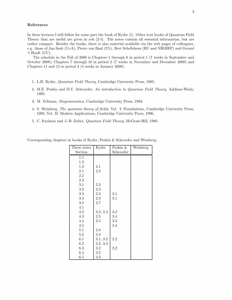
In these lectures I will follow for some part the book of Ryder [1]. Other text books of Quantum FieldTheory that are useful are given in refs [2-5]. The notes contain all essential information, but arerather compact. Besides the books, there is also material available via the web pages of colleagues,e.g. those of Jan Smit (UvA), Pierre van Baal (UL), Bert Schellekens (RU and NIKHEF) and Gerard’t Hooft (UU).
The schedule in the Fall of 2008 is Chapters 1 through 6 in period 1 (7 weeks in September andOctober 2008), Chapters 7 through 10 in period 2 (7 weeks in November and December 2008) andChapters 11 and 12 in period 3 (4 weeks in January 2009).
1. L.H. Ryder, Quantum Field Theory, Cambridge University Press, 1985.
2. M.E. Peskin and D.V. Schroeder, An introduction to Quantum Field Theory, Addison-Wesly,1995.
3. M. Veltman, Diagrammatica, Cambridge University Press, 1994.
4. S. Weinberg, The quantum theory of fields; Vol. I: Foundations, Cambridge University Press,1995; Vol. II: Modern Applications, Cambridge University Press, 1996.
5. C. Itzykson and J.-B. Zuber, Quantum Field Theory, McGraw-Hill, 1980.
Corresponding chapters in books of Ryder, Peskin & Schroeder and Weinberg.
These notes Ryder Peskin & WeinbergSection Schroeder
1.11.21.3 2.12.1 2.22.22.33.1 2.33.2 2.33.3 2.3 3.13.4 2.3 3.13.5 2.74.14.2 2.3, 2.4 3.24.3 2.5 3.44.4 2.5 3.34.5 3.45.1 2.85.2 3.46.1 3.1, 3.2 2.26.2 3.2, 3.36.3 3.2 2.26.4 3.26.5 3.3
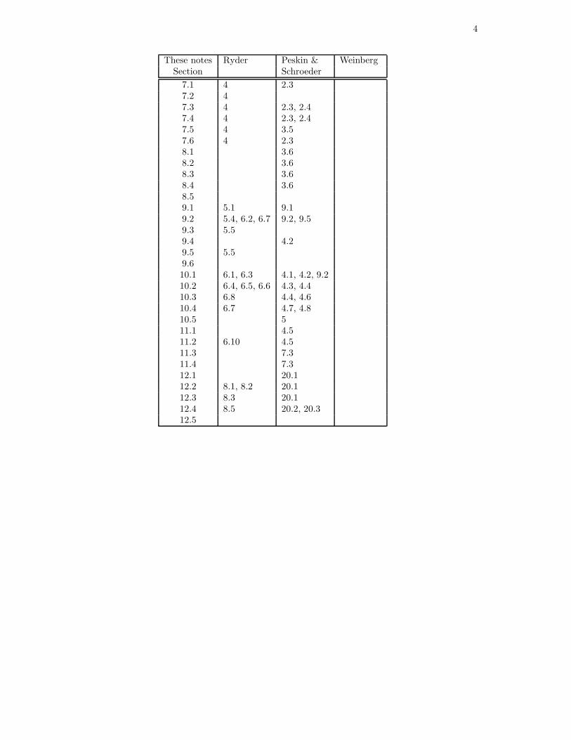
4
These notes Ryder Peskin & WeinbergSection Schroeder
7.1 4 2.37.2 47.3 4 2.3, 2.47.4 4 2.3, 2.47.5 4 3.57.6 4 2.38.1 3.68.2 3.68.3 3.68.4 3.68.59.1 5.1 9.19.2 5.4, 6.2, 6.7 9.2, 9.59.3 5.59.4 4.29.5 5.59.610.1 6.1, 6.3 4.1, 4.2, 9.210.2 6.4, 6.5, 6.6 4.3, 4.410.3 6.8 4.4, 4.610.4 6.7 4.7, 4.810.5 511.1 4.511.2 6.10 4.511.3 7.311.4 7.312.1 20.112.2 8.1, 8.2 20.112.3 8.3 20.112.4 8.5 20.2, 20.312.5

5
Chapter 1
Introduction
1.1 Quantum field theory
In quantum field theory the theories of quantum mechanics and special relativity are united. Inquantum mechanics a special role is played by Planck’s constant h, usually given divided by 2π,
h ≡ h/2π = 1.054 571 68 (18) × 10−34 J s
= 6.582 119 15 (56) × 10−22 MeV s. (1.1)
In the limit that the action S is much larger than h, S ≫ h, quantum effects do not play a roleanymore and one is in the classical domain. In special relativity a special role is played by the velocityof light c,
c = 299 792 458 m s−1. (1.2)
In the limit that v ≪ c one reaches the non-relativistic domain.In the framework of classical mechanics as well as quantum mechanics the position of a particle
is a well-defined concept and the position coordinates can be used as dynamical variables in thedescription of the particles and their interactions. In quantum mechanics, the position can in principlebe determined at any time with any accuracy, being eigenvalues of the position operators. One cantalk about states |r〉 and the wave function ψ(r) = 〈r||ψ〉. In this coordinate representation theposition operators rop simply acts as
rop ψ(r) = r ψ(r). (1.3)
The uncertainty principle tells us that in this representation the momenta cannot be fully determined.Corresponding position and momentum operators do not commute. They satisfy the well-known(canonical) operator commutation relations
[ri, pj ] = ih δij , (1.4)
where δij is the Kronecker δ function. Indeed, the action of the momentum operator in the coordinaterepresentation is not as simple as the position operator. It is given by
popψ(r) = −ih∇ψ(r). (1.5)
One can also choose a representation in which the momenta of the particles are the dynamical variables.The corresponding states are |p〉 and the wave functions ψ(p) = 〈p||ψ〉 are the Fourier transforms ofthe coordinate space wave functions,
ψ(p) =
∫
d3r exp
(
− i
hp · r
)
ψ(r), (1.6)
1
Introduction 2
and
ψ(r) =
∫d3p
(2πh)3exp
(i
hp · r
)
ψ(p). (1.7)
The existence of a limiting velocity, however, leads to new fundamental limitations on the possiblemeasurements of physical quantities. Let us consider the measurement of the position of a particle.This position cannot be measured with infinite precision. Any device that wants to locate the positionof say a particle within an interval ∆x will contain momentum components p ∝ h/∆x. Therefore ifwe want ∆x ≤ h/mc (where m is the rest mass of the particle), momenta of the order p ∝ mc andenergies of the order E ∝ mc2 are involved. It is then possible to create a particle - antiparticle pairand it is no longer clear of which particle we are measuring the position. As a result, we find that theoriginal particle cannot be located better than within a distance h/mc, its Compton wavelength,
∆x ≥ h
mc. (1.8)
For a moving particle mc2 → E (or by considering the Lorentz contraction of length) one has ∆x ≥hc/E. If the particle momentum becomes relativistic, one has E ≈ pc and ∆x ≥ h/p, which says thata particle cannot be located better than its de Broglie wavelength.Thus the coordinates of a particle cannot act as dynamical variables (since these must have a precisemeaning).
Some consequences are that only in cases where we restrict ourselves to distances ≫ h/mc, theconcept of a wave function becomes a meaningful (albeit approximate) concept. For a massless particleone gets ∆x ≫ h/p = λ/2π, i.e. the coordinates of a photon only become meaningful in cases wherethe typical dimensions are much larger than the wavelength.
For the momentum or energy of a particle we know that in a finite time ∆t, the energy uncertaintyis given by ∆E ≥ h/∆t. This implies that the momenta of particles can only be measured exactlywhen one has an infinite time available. For a particle in interaction, the momentum changes with timeand a measurement over a long time interval is meaningless. The only case in which the momentumof a particle can be measured exactly is when the particle is free and stable against decay. In this casethe momentum is conserved and one can let ∆t become infinitely large.
The result thus is that the only observable quantities that can serve as dynamical coordinates arethe momenta (and further the internal degrees of freedom like polarizations, . . . ) of free particles.These are the particles in the initial and final state of a scattering process. The theory will not givean observable meaning to the time dependence of interaction processes. The description of such aprocess as occurring in the course of time is just as unreal as classical paths are in non-relativisticquantum mechanics.
The main problem in Quantum Field Theory is to determine the probability amplitudes be-tween well-defined initial and final states of a system of free particles. The set of such amplitudes〈p′1,p′2; out|p1,p2; in〉 ≡ 〈p′1,p′2; in|S|p1,p2; in〉 determines the scattering matrix or S-matrix.
Another point that needs to be emphasized is the meaning of particle in the above context. Actu-ally, the better name might be ’degree of freedom’. If the energy is low enough to avoid excitation ofinternal degrees of freedom, an atom is a perfect example of a particle. In fact, it is the behavior underPoincare transformations or in the limit v ≪ c Gallilei transformations that determine the descriptionof a particle state, in particular the free particle state.
1.2 Units
It is important to choose an appropriate set of units when one considers a specific problem, becausephysical sizes and magnitudes only acquire a meaning when they are considered in relation to eachother. This is true specifically for the domain of atomic, nuclear and high energy physics, wherethe typical numbers are difficult to conceive on a macroscopic scale. They are governed by a fewfundamental units and constants, which have been discussed in the previous section, namely h and
Introduction 3
c. By making use of these fundamental constants, we can work with less units. For instance, thequantity c is used to define the meter. We could as well have set c = 1. This would mean that one ofthe two units, meter or second, is eliminated, e.g. given a length l the quantity l/c has the dimensionof time and one finds 1 m = 0.33× 10⁻⁸ s or eliminating the second one would use that, given a timet, the quantity ct has dimension of length and hence 1 s = 3 × 10⁸ m.
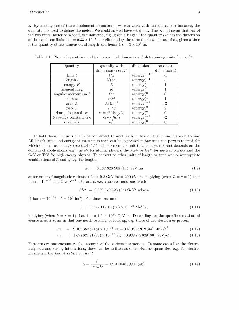
Table 1.1: Physical quantities and their canonical dimensions d, determining units (energy)d.
quantity quantity with dimension canonicaldimension energyd dimension d
time t t/h (energy)−1 -1length l l/(hc) (energy)−1 -1energy E E (energy)1 1
momentum p pc (energy)1 1angular momentum ℓ ℓ/h (energy)0 0
mass m mc2 (energy)1 1area A A/(hc)2 (energy)−2 -2force F F hc (energy)2 2
charge (squared) e2 α = e2/4πǫ0 hc (energy)0 0Newton’s constant GN GN/(hc
5) (energy)−2 -2velocity v v/c (energy)0 0
In field theory, it turns out to be convenient to work with units such that h and c are set to one.All length, time and energy or mass units then can be expressed in one unit and powers thereof, forwhich one can use energy (see table 1.1). The elementary unit that is most relevant depends on thedomain of applications, e.g. the eV for atomic physics, the MeV or GeV for nuclear physics and theGeV or TeV for high energy physics. To convert to other units of length or time we use appropriatecombinations of h and c, e.g. for lengths
hc = 0.197 326 968 (17) GeV fm (1.9)
or for order of magnitude estimates hc ≈ 0.2 GeV fm = 200 eVnm, implying (when h = c = 1) that1 fm = 10−15 m ≈ 5 GeV−1. For areas, e.g. cross sections, one needs
h2c2 = 0.389 379 323 (67) GeV2 mbarn (1.10)
(1 barn = 10−28 m2 = 102 fm2). For times one needs
h = 6.582 119 15 (56) × 10−22 MeV s, (1.11)
implying (when h = c = 1) that 1 s ≈ 1.5 × 1024 GeV−1. Depending on the specific situation, ofcourse masses come in that one needs to know or look up, e.g. those of the electron or proton,
me = 9.109 382 6 (16)× 10−31 kg = 0.510 998 918 (44) MeV/c2, (1.12)
mp = 1.672 621 71 (29)× 10−27 kg = 0.938 272 029 (80) GeV/c2. (1.13)
Furthermore one encounters the strength of the various interactions. In some cases like the electro-magnetic and strong interactions, these can be written as dimensionless quantities, e.g. for electro-magnetism the fine structure constant
α =e2
4π ǫ0 hc= 1/137.035 999 11 (46). (1.14)
Introduction 4
For weak interactions and gravity one has quantities with a dimension, e.g. for gravity Newton’sconstant,
GN
hc5= 6.708 7 (10)× 10−39 GeV−2. (1.15)
By putting this quantity equal to 1, one can also eliminate the last dimension. All masses, lengthsand energies are compared with the Planck mass or length (see exercises). Having many particles,the concept of temperature becomes relevant. A relation with energy is established via the averageenergy of a particle being of the order of kT , with the Boltzmann constant given by
k = 1.380 650 5(24)× 10−23 J/K = 8.617 343(15)× 10−5 eV/K. (1.16)
Quantities that do not contain h or c are classical quantities, e.g. the mass of the electron me.Quantities that contain only h are expected to play a role in non-relativistic quantum mechanics,e.g. the Bohr radius, a∞ = 4πǫ0h
2/mee2 or the Bohr magneton µe = eh/2me. Quantities that only
contain c occur in classical relativity, e.g. the electron rest energy mec2 and the classical electron
radius re = e2/4πǫ0 mec2. Quantities that contain both h and c play a role in relativistic quantum
mechanics, e.g. the electron Compton wavelength −λe = h/mec. It remains useful, however, to use hand c to simplify the calculation of quantities.
1.3 Conventions for vectors and tensors
We start with vectors in Euclidean 3-space E(3). A vector x can be expanded with respect to a basisei (i = 1, 2, 3 or i = x, y, z),
x =
3∑
i=1
xi ei = xi ei, (1.17)
to get the three components of a vector, xi. When a repeated index appears, such as on the righthand side of this equation, summation over this index is assumed (Einstein summation convention).Choosing an orthonormal basis, the metric in E(3) is given by ei · ej = δij , where the Kronecker deltais given by
δij =
1 if i = j0 if i 6= j,
. (1.18)
The inner product of two vectors is given by
x · y = xi yi ei · ej = xi yj δij = xiyi. (1.19)
The inner product of a vector with itself gives its length squared. A vector can be rotated, x′ = Rx
or x′i = Rijxj leading to a new vector with different components. Actually, rotations are those real,linear transformations that do not change the length of a vector. Tensors of rank n are objects with ncomponents that transform according to T ′i1...in
= Ri1j1 . . . RinjnTj1...jn
. A vector is a tensor of rank1. The inner product of two vectors is a rank 0 tensor or scalar. The Kronecker delta is a constantrank-2 tensor. It is an invariant tensor that does not change under rotations. The only other invariantconstant tensor in E(3) is the Levi-Civita tensor
ǫijk =
1 if ijk is an even permutation of 123−1 if ijk is an odd permutation of 1230 otherwise.
(1.20)
that can be used in the cross product of two vectors z = x × y, in which case zi = ǫijk xjyk. Usefulrelations are
ǫijk ǫimn = δjm δkn − δjn δkm, (1.21)
ǫijk ǫijl = 2 δkl. (1.22)
Introduction 5
We note that for Euclidean spaces (with a positive definite metric) vectors and tensors there is onlyone type of indices. No difference is made between upper or lower. So we could have used all upperindices in the above equations. When 3-dimensional space is considered as part of Minkowski space,however, we will use upper indices for the three-vectors.
In special relativity we start with a four-dimensional real vector space E(1,3) with basis nµ (µ =0,1,2,3). Vectors are denoted x = xµnµ. The length (squared) of a vector is obtained from the scalarproduct,
x2 = x · x = xµxν nµ · nν = xµxνgµν . (1.23)
The quantity gµν ≡ nµ · nν is the metric tensor, given by g00 = −g11 = −g22 = −g33 = 1 (theother components are zero). For four-vectors in Minkowski space we will use the notation with upperindices and write x = (t,x) = (x0, x1, x2, x3), where the coordinate t = x0 is referred to as the timecomponent, xi are the three space components. Because of the different signs occurring in gµν , it isconvenient to distinguish lower indices from upper indices. The lower indices are constructed in thefollowing way, xµ = gµνx
ν , and are given by (x0, x1, x2, x3) = (t,−x). One has
x2 = xµxµ = t2 − x2. (1.24)
The scalar product of two different vectors x and y is denoted
x · y = xµyνgµν = xµyµ = xµyµ = x0y0 − x · y. (1.25)
Within Minkowski space the real, linear transformations that do not change the length of a four-vectorare called the Lorentz transformations. These transformations do change the components of a vector,denoted as V ′µ = Λµ
ν Vν , The (invariant) lengths often have special names, such as eigentime τ for the
position vector τ2 ≡ x2 = t2 − x2. The invariant distance between two points x and y in Minkowskispace is determined from the length dsµ = (x − y)µ. The real, linear transformations that leave thelength of a vector invariant are called (homogeneous) Lorentz transformations. The transformationsthat leave invariant the distance ds2 = dt2 − (dx2 + dy2 + dz2) between two points are called inhomo-geneous Lorentz transformations or Poincare transformations. The Poincare transformations includeLorentz transformations and translations.
Unlike in Euclidean space, the invariant length or distance (squared) is not positive definite. Onecan distinguish:
• ds2 > 0 (timelike intervals); in this case an inertial system exists in which the two points are atthe same space point and in that frame ds2 just represents the time difference ds2 = dt2;
• ds2 < 0 (spacelike intervals); in this case an inertial system exists in which the two points areat the same time and ds2 just represents minus the spatial distance squred ds2 = −dx2;
• ds2 = 0 (lightlike or null intervals); the points lie on the lightcone and they can be connectedby a light signal.
Many other four vectors and tensors transforming like T ′µ1...µn = Λµ1ν1. . .Λµn
νnT ν1...νn can be con-
structed. In Minkowski space, one must distinguish tensors with upper or lower indices and one canhave mixed tensors. Relations relating tensor expressions, independent of a coordinate system, arecalled covariant. Examples are the scalar products above but also relations like pµ = mdxµ/dτ for themomentum four vector. Note that in this equation one has on left- and righthandside a four vectorbecause τ is a scalar quantity! The equation with t = x0 instead of τ simply would not make sense!The momentum four vector, explicitly written as (p0,p) = (E,p), is timelike with invariant length(squared) p2 = p · p = pµpµ = E2 − p2 = m2, where m is called the mass of the system.
The derivative ∂µ is defined ∂µ = ∂/∂xµ and we have a four vector ∂ with components
(∂0, ∂1, ∂2, ∂3) =
(∂
∂t,∂
∂x,∂
∂y,∂
∂z
)
=
(∂
∂t,∇
)
. (1.26)
Introduction 6
It is easy to convince oneself of the nature of the indices in the above equation, because one has
∂µ xν = gν
µ. (1.27)
Note that gνµ with one upper and lower index, constructed via the metric tensor itself, gν
µ = gµρgρν and
is in essence a ’Kronecker delta’, g00 = g1
1 = g22 = g3
3 = 1. The length squared of ∂ is the d’Alembertianoperator, defined by
2 = ∂µ∂µ =∂2
∂t2− ∇
2. (1.28)
The value of the antisymmetric tensor ǫµνρσ is determined in the same way as for ǫijk, startingfrom
ǫ0123 = 1. (1.29)
(Note that there are different conventions around and sometimes the opposite sign is used). It is aninvariant tensor, not affected by Lorentz transformations. The product of two epsilon tensors is givenby
ǫµνρσǫµ′ν′ρ′σ′
= −
∣∣∣∣∣∣∣∣
gµµ′
gµν′
gµρ′
gµσ′
gνµ′
gνν′
gνρ′
gνσ′
gρµ′
gρν′
gρρ′
gρσ′
gσµ′
gσν′
gσρ′
gσσ′
∣∣∣∣∣∣∣∣
, (1.30)
ǫµνρσǫ ν′ρ′σ′
µ = −
∣∣∣∣∣∣
gνν′
gνρ′
gνσ′
gρν′
gρρ′
gρσ′
gσν′
gσρ′
gσσ′
∣∣∣∣∣∣
, (1.31)
ǫµνρσǫ ρ′σ′
µν = −2(
gρρ′
gσσ′ − gρσ′
gσρ′)
, (1.32)
ǫµνρσǫ σ′
µνρ = −6gσσ′
, (1.33)
ǫµνρσǫµνρσ = −24. (1.34)
The first identity, for instance, is easily proven for ǫ0123 ǫ0123 from which the general case can beobtained by making permutations of indices on the lefthandside and permutations of rows or columnson the righthandside. Each of these permutations leads to a minus sign, but more important has thesame effect on lefthandside and righthandside. For the contraction of a vector with the antisymmetrictensor one often uses the shorthand notation
ǫABCD = ǫµνρσAµBνCρDσ. (1.35)
Exercises
Exercise 1.1
(a) In the the Hydrogen atom (quantum system) the scale is set by the Bohr radius, a∞ =4πǫ0h
2/mee2. Relate this quantity to the electron Compton wavelength −λe via the dimensionless
fine structure constant α.
(b) Relate the classical radius of the electron (a relativistic concept), re = e2/4πǫ0 mec2 to the
Compton wavelength.
(c) Calculate the Compton wavelength of the electron and the quantities under (a) and (b) usingthe value of hc, α and mec
2 = 0.511 MeV. This demonstrates how a careful use of units can savea lot of work. One does not need to know h, c, ǫ0, me, e, but only appropriate combinations.
Introduction 7
(d) Use the value of the gravitational constant GN/hc5 = 6.71 × 10−39 GeV−2 to construct a mass
Mpl (Planck mass). Compare it with the proton mass and use Eq. 1.13 to give its actual valuein kg. Also construct and calculate the Planck length Lpl, which is the Compton wavelength forthe Planck mass.
(e) Find a simple way (avoiding putting in the value of e) to calculate the Bohr magneton µe =eh/2me and the nuclear magneton µp = eh/2mp in electronvolt per Tesla (eV/T ).[Note: what is the MKS unit for V/T?]
Exercise 1.2
Prove the identity A× (B ×C) = (A ·C)B - (A ·B)C using the properties of the tensor ǫijk givenin section 1.3.
Exercise 1.3
Prove the following relation
ǫµνρσ gαβ = ǫανρσ gµβ + ǫµαρσ gνβ + ǫµνασ gρβ + ǫµνρα gσβ .
by a simple few-line reasoning [For instance: If µ, ν, ρ, σ is a permutation of 0, 1, 2, 3 the index αcan only be equal to one of the indices in ǫµνρσ, . . . ].
Exercise 1.4
Lightcone coordinates for a four vector a (which we will denote with square brackets as [a−, a+, a1, a2]or [a−, a+,aT ]) are defined through
a± ≡ (a0 ± a3)/√
2.
(a) Express the scalar product a · b in lightcone coordinates and deduce from this the values of g++,g−−, g+− and g−+.
(b) Check that the following vectors n0, n3, n+ and n−,
n0 = (1, 0, 0, 0)
n3 = (0, 0, 0, 1)
n+ = (1, 0, 0, 1)/√
2 = (n0 + n3)/√
2
n− = (1, 0, 0,−1)/√
2 = (n0 − n3)/√
2
can be used to obtain the corresponding components of a four vector, i.e. a · nα = aα. Thisimplies that the components of nα are given by nµ
α = gµα.
Chapter 2
Relativistic wave equations
2.1 The Klein-Gordon equation
In this chapter, we just want to play a bit with covariant equations and study their behavior underLorentz transformations. The Schrodinger equation in quantum mechanics is the operator equationcorresponding to the non-relativistic expression for the energy,
E =p2
2M, (2.1)
under the substitution (in coordinate representation)
E −→ Eop = i∂
∂t, p −→ pop = −i∇. (2.2)
Acting on the wave function one finds for a free particle,
i∂
∂tψ(r, t) = − ∇
2
2Mψ(r, t). (2.3)
Equations 2.1 and 2.3 are not covariant. But the replacement 2.2, written as pµ −→ i∂µ is covariant(the same in every frame of reference). Thus a covariant equation can be obtained by starting withthe (covariant) equation for the invariant length of the four vector (E,p),
p2 = pµpµ = E2 − p2 = M2, (2.4)
where M is the particle mass. Substitution of operators gives the Klein-Gordon (KG) equation for areal or complex function φ,
(2 +M2
)φ(r, t) =
(∂2
∂t2− ∇
2 +M2
)
φ(r, t) = 0. (2.5)
Although it is straightforward to find the solutions of this equation, namely plane waves characterizedby a wave number k,
φk(r, t) = exp(−i k0t+ ik · r), (2.6)
with (k0)2 = k2 +M2, the interpretation of this equation as a single-particle equation in which φ is acomplex wave function poses problems because the energy spectrum is not bounded from below andthe probability is not positive definite.
• The energy spectrum is not bounded from below: considering the above stationary plane wavesolutions one obtains
k0 = ±√
k2 +M2 = ±Ek, (2.7)
i.e. there are solutions with negative energy.
8
Relativistic wave equations 9
• Probability is not positive: in quantum mechanics one has the probability and probability current
ρ = ψ∗ψ (2.8)
j = − i
2M(ψ∗∇ψ − (∇ψ∗)ψ) ≡ − i
2Mψ∗↔∇ ψ. (2.9)
They satisfy the continuity equation,
∂ρ
∂t= −∇ · j, (2.10)
which follows directly from the Schrodinger equation. This continuity equation can be writtendown covariantly using the components (ρ, j) of the four-current j,
∂µjµ = 0. (2.11)
Therefore, relativistically the density is not a scalar quantity, but rather the zero component ofa four vector. The appropriate current corresponding to the KG equation (see Excercise 2.2) is
jµ = i φ∗↔∂µ φ or (ρ, j) =
(
i φ∗↔∂0 φ,−i φ∗
↔∇ φ
)
. (2.12)
It is easy to see that this current is conserved if φ (and φ∗) satisfy the KG equation. The KGequation, however, is a second order equation and φ and ∂φ/∂t can be fixed arbitrarily at agiven time. This leads to the existence of negative densities.
As we will see both problems are related and have to do with the existence of particles and antiparticles,for which we need the interpretation of φ as a field that must be quantized. Besides a wave functionthe field must be an operator. Its argument, the position r simply becomes a number (parameter) onwhich the operator depend, very much similar as the time t. Then, there are no longer fundamentalobjections to mix up space and time, which is what Lorentz transformations do. And, it is simply amatter of being careful to find a consistent (covariant) theory.
2.2 Mode expansion of solutions of the KG equation
Before quantizing fields, having the KG equation as a space-time symmetric (classical) equation, wenote that an arbitrary solution for the field φ can always be written as a superposition of plane waves,
φ(x) =
∫d4k
(2π)42π δ(k2 −M2) e−i k·x φ(k) (2.13)
with (in principle complex) coefficients φ(k). The integration over k-modes clearly is covariant andrestricted to the ‘mass’-shell (as required by Eq. 2.5). It is possible to rewrite it as an integration overpositive energies only but this gives two terms (use the result of exercise 2.3),
φ(x) =
∫d3k
(2π)3 2Ek
(
e−i k·x φ(Ek,k) + ei k·x φ(−Ek,−k))
. (2.14)
Introducing φ(Ek,k) ≡ a(k) and φ(−Ek,−k) ≡ b∗(k) one has
φ(x) =
∫d3k
(2π)3 2Ek
(e−i k·x a(k) + ei k·x b∗(k)
)= φ+(x) + φ−(x). (2.15)
In Eqs 2.14 and 2.15 one has elimated k0 and in both equations k · x = Ekt− k · x. The coefficientsa(k) and b∗(k) are the amplitudes of the two independent solutions (two, after restricting the energiesto be positive). They are referred to as mode and anti-mode amplitudes (or because of their originpositive and negative energy modes). The choice of a and b∗ allows an easier distinction between thecases that φ is real (a = b) or complex (a and b are independent amplitudes).
Relativistic wave equations 10
2.3 Symmetries of the Klein-Gordon equation
We arrived at the Klein-Gordon equation by constructing a covariant operator (∂µ∂µ + M2) acting
on a complex function φ. Performing some Lorentz transformation x→ x′ = Λx, one thus must havethat the function φ→ φ′ such that
φ′(x′) = φ(x) or φ′(x) = φ(Λ−1x). (2.16)
The consequence of this is discussed in Exercise 2.3We will explicitly discuss the example of a discrete symmetry, for which we consider space inversion,
i.e. changing the sign of the spatial coordinates, which implies
(xµ) = (t,x) → (t,−x) ≡ (xµ). (2.17)
Transforming everywhere in the KG equation x→ x one obtains
(
∂µ∂µ +M2
)
φ(x) = 0. (2.18)
Since a · b = a · b, it is easy to see that
(∂µ∂
µ +M2)φ(x) = 0, (2.19)
implying that for each solution φ(x) there exists a corresponding solution with the same energy,φP (x) ≡ φ(x) (P for parity). It is easy to show that
φP (x) = φ(x) =
∫d3k
(2π)3 2Ek
(e−i k·x a(k) + ei k·x b∗(k)
)
=
∫d3k
(2π)3 2Ek
(
e−i k·x a(k) + ei k·x b∗(k))
=
∫d3k
(2π)3 2Ek
(e−i k·x a(−k) + ei k·x b∗(−k)
), (2.20)
or since one can define
φP (x) ≡∫
d3k
(2π)3 2Ek
(e−i k·x aP (k) + ei k·x bP∗(k)
), (2.21)
one has for the mode amplitudes aP (k) = a(−k) and bP (k) = b(−k). This shows how parity trans-forms k-modes into −k modes.
Another symmetry is found by complex conjugating the KG equation. It is trivial to see that
(∂µ∂
µ +M2)φ∗(x) = 0, (2.22)
showing that with each solution there is a corresponding charge conjugated solution φC(x) = φ∗(x).In terms of modes one has
φC(x) = φ∗(x) =
∫d3k
(2π)3 2Ek
(e−i k·x b(k) + ei k·x a∗(k)
)
≡∫
d3k
(2π)3 2Ek
(e−i k·x aC(k) + ei k·x bC∗(k)
), (2.23)
i.e. for the mode amplitudes aC(k) = b(k) and bC(k) = a(k). For the real field one has aC(k) = a(k).This shows how charge conjugation transforms ’particle’ modes into ’antiparticle’ modes and viceversa.
Relativistic wave equations 11
Exercises
Exercise 2.1
Show that for a conserved current (∂µjµ = 0) the charge in a finite volume, QV ≡
∫
V d3x j0(x),
satisfies
QV = −∫
S
ds · j,
and thus for any normalized solution the full ‘charge’, letting V → ∞, is conserved, Q = 0.
Exercise 2.2
Show that if φ en φ∗ are solutions of the KG equation, that
jµ = i φ∗↔∂µ φ
is a conserved current
Note: A↔∂µ B ≡ A∂µB − (∂µA)B).
Exercise 2.3
Show that1 ∫d4k
(2π)42π δ(k2 −M2) θ(k0) F (k0,k) =
∫d3k
(2π)3 2EkF (Ek,k),
where Ek =√
k2 +M2.
Exercise 2.4
Derive from the mode expansion in Eq. 2.15, the 3-dimensional Fourier transform φ(k, t) ≡∫d3x φ(x, t) exp(−ik·
x) and its time derivative i∂0φ(k, t). Use these to show that
a(k) = ei Ekt i↔∂0 φ(k, t) = ei Ekt (i∂0 + Ek) φ(k, t),
b(k) = ei Ekt i↔∂0 φ∗(−k, t),
Note that a(k) and b(k) are independent of t.
Exercise 2.5
Express the full charge QV (exercise 2.1) for a complex scalar field current (exercise 2.2) in terms ofthe a(k) and b(k) using the expansion in Eq. 2.15.
Similarly express the quantities
E =
∫
d3x((∂0φ)∗(∂0φ) + ∇φ∗ · ∇φ+M2φ∗φ
),
P i =
∫
d3x (∂0φ)∗(∂iφ),
1Use the following property of delta functions
δ (f(x)) =X
zeros xn
1
|f ′(xn)| δ(x − xn).
Relativistic wave equations 12
in terms of the a(k) and b(k). Note that aµbν indicates symmetrization, aµbν ≡ aµbν + aνbµ. Wewill encounter these quantities later as energy and momentum.
Note: Do not repeat all steps, but realize which ones are common to the calculations. As an in-termediate step you could also calculate for two field φ1 (with coefficients a1 and b∗1) and φ2 (withcoefficients a2 and b∗2) the integral
∫
d3x φ∗1(x)φ2(x) =
∫d3k
(2π)3 4E2k
(
a∗1(k)a2(k) + b1(k)b∗2(k)
+ a∗1(k)b∗2(−k) e2iEkt + b1(k)a2(−k) e−2iEkt
)
.
Exercise 2.6 (optional)
Write down the mode expansion for the Lorentz transformed scalar field φ′(x) and show that it impliesthat the Lorentz transformed modes are a′(k) = a(k′), where k′ = Λ−1k with k = (Ek,k).
Chapter 3
Groups and their representations
Simple systems that ought to be described with relativistic equations are free particles with spin, e.g.electrons. In this section we will investigate if there exist objects other than just a scalar (real orcomplex) field φ, e.g. two-component fields in analogy to the two-component wave functions used toinclude spin in a quantum mechanical description of an electron in the atom.
Since the KG equation expresses just the relativistic relation between energy and momentum, italso must hold for particles with spin. However, since the symmetry group describing rotations isembedded in the Lorentz group, we must study the representations of the Lorentz group. Particleswith spin then will be described by certain spinors. The KG equation will actually remain valid, inparticular each component of these spinors will satisfy this equation.
Before proceeding with the Lorentz group we will first discuss the rotation group as an exampleof a Lie group with which we are familiar in ordinary quantum mechanics.
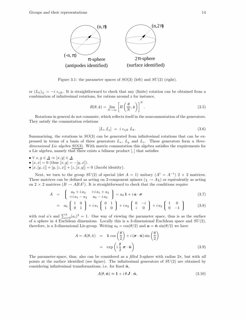
3.1 The rotation group and SU(2)
The rotation groups SO(3) and SU(2) are examples of Lie groups, that is groups characterized by afinite number of real parameters, in which the parameter space forms locally a Euclidean space. Ageneral rotation — we will consider SO(3) as an example — is of the form
V ′xV ′yV ′z
=
cos θ sin θ 0− sin θ cos θ 0
0 0 1
Vx
Vy
Vz
(3.1)
for a rotation around the z-axis or shorthand V ′ = R(θ, z)V . The parameter-space of SO(3) is asphere with radius π. Any rotation can be uniquely written as R(θ, n) where n is a unit vector andθ is the rotation angle, 0 ≤ θ ≤ π, provided we identify the antipodes, i.e. R(π, n) ≡ R(π,−n).Locally this parameter-space is 3-dimensional and correspondingly one has three generators. For aninfinitesimal rotation around the z-axis one has
R(θ, z) = 1 + i δθ Lz (3.2)
with as generator
Lz =1
i
∂R(θ, z)
∂θ
∣∣∣∣θ=0
=
0 −i 0i 0 00 0 0
. (3.3)
In the same way we can consider rotations around the x- and y-axes that are generated by
Lx =
0 0 00 0 −i0 i 0
, Ly =
0 0 i0 0 0−i 0 0
, (3.4)
13
Groups and their representations 14
(n, )
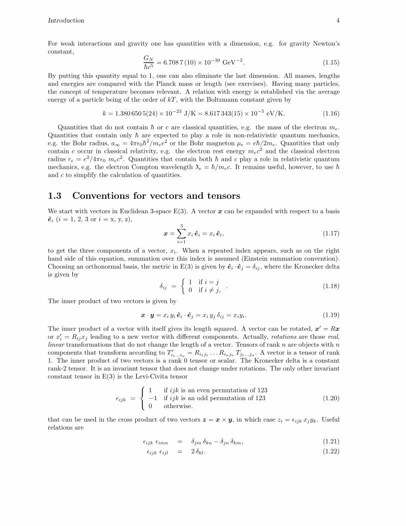
-sphere -sphere
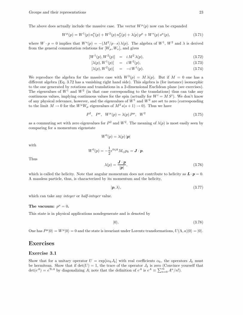
(n,2 )π
π π
π
π 2(antipodes identified) (surface identified)
(-n, )
Figure 3.1: the parameter spaces of SO(3) (left) and SU(2) (right).
or (Lk)ij = −i ǫijk. It is straightforward to check that any (finite) rotation can be obtained from acombination of infinitesimal rotations, for rations around z for instance,
R(θ, z) = limN→∞
[
R
(θ
N, z
)]N
. (3.5)
Rotations in general do not commute, which reflects itself in the noncommutation of the generators.They satisfy the commutation relations
[Li, Lj] = i ǫijk Lk. (3.6)
Summarizing, the rotations in SO(3) can be generated from infinitesimal rotations that can be ex-pressed in terms of a basis of three generators Lx, Ly and Lz. These generators form a three-dimensional Lie algebra SO(3). With matrix commutation this algebra satisfies the requirements fora Lie algebra, namely that there exists a bilinear product [, ] that satisfies
• ∀ x, y ∈ A⇒ [x, y] ∈ A.• [x, x] = 0 (thus [x, y] = −[y, x]).• [x, [y, z]] + [y, [z, x]] + [z, [x, y]] = 0 (Jacobi identity).
Next, we turn to the group SU(2) of special (det A = 1) unitary (A† = A−1) 2 × 2 matrices.These matrices can be defined as acting on 2-component spinors (χ → Aχ) or equivalently as actingon 2 × 2 matrices (B → ABA†). It is straightforward to check that the conditions require
A =
a0 + i a3 +i a1 + a2
+i a1 − a2 a0 − i a3
= a0 1 + ia · σ (3.7)
= a0
1 00 1
+ i a1
0 11 0
+ i a2
0 −ii 0
+ i a3
1 00 −1
(3.8)
with real a’s and∑3
i=0(ai)2 = 1. One way of viewing the parameter space, thus is as the surface
of a sphere in 4 Euclidean dimensions. Locally this is a 3-dimensional Euclidean space and SU(2),therefore, is a 3-dimensional Lie-group. Writing a0 = cos(θ/2) and a = n sin(θ/2) we have
A = A(θ, n) = 1 cos
(θ
2
)
+ i (σ · n) sin
(θ
2
)
= exp
(
iθ
2σ · n
)
(3.9)
The parameter-space, thus, also can be considered as a filled 3-sphere with radius 2π, but with allpoints at the surface identified (see figure). The infinitesimal generators of SU(2) are obtained byconsidering infinitesimal transformations, i.e. for fixed n,
A(θ, n) ≈ 1 + i θ J · n, (3.10)

Groups and their representations 15
with
J · n ≡ 1
i
∂A(θ, n)
∂θ
∣∣∣∣θ=0
=σ
2· n. (3.11)
Thus σx/2, σy/2 and σz/2 form the basis of the Lie-algebra SU(2). They satisfy
[σi
2,σj
2] = i ǫijk
σk
2. (3.12)
One, thus, immediately sees that the Lie algebras are identical, SU(2) ≃ SO(3), i.e. one has a Liealgebra isomorphism that is linear and preserves the bilinear product.
There exists a corresponding mapping of the groups given by
µ : SU(2) −→ SO(3)
A(θ, n) −→ R(θ, n) 0 ≤ θ ≤ π
−→ R(2π − θ, n) π ≤ θ ≤ 2π.
The relationA(σ · a)A−1 = σ ·RAa (3.13)
can be used to establish the homomorphism (Check that it satisfies the requirements of a homomor-phism). Near the identity, the above mapping corresponds to the trivial mapping of the Lie algebras.In the full parameter space, however, the SU(2) → SO(3) mapping is a 2 : 1 mapping where bothA = ±1 are mapped into R = I.
3.2 Representations of symmetry groups
The presence of symmetries simplifies the description of a physical system. Suppose we have a systemdescribed by a HamiltonianH . The existence of symmetries means that there are operators g belongingto a symmetry group G that commute with the Hamiltonian,
[g,H ] = 0 for g ∈ G. (3.14)
For a Lie group, it is sufficient that the generators commute with H , since any finite rotation can beconstructed from the infinitesimal ones, sometimes in more than one way (but this will be discussedlater), i.e.
[g,H ] = 0 for g ∈ G. (3.15)
Representations Φ of a group are mappings of G into a finite dimensional vector space, preservingthe group structure. In order to find local representations Φ of a Lie-group G, it is sufficient to considerthe representations Φ of the Lie-algebra G. These are mappings from G into a finite dimensionalvector space (its dimension is the dimension of the representation), which preserve the Lie-algebrastructure, i.e. the commutation relations. Among the generators one looks for a maximal commutingset of operators (in this case consisting of the operator Jz and the (quadratic Casimir) operatorJ2). Casimir operators commute with all the generators and the eigenvalue of J2 can be used tolabel the representation (j). Within the (2j + 1)-dimensional representation space V (j) one can labelthe eigenstates |j,m〉 with eigenvalues of Jz. The other generators Jx and Jy (or J± ≡ Jx ± iJy)then transform between the states in V (j). From the algebra one derives J2|j,m〉 = j(j + 1)|j,m〉,Jz|j,m〉 = m|j,m〉, while J±|j,m〉 =
√
j(j + 1) −m(m± 1)|j,m ± 1〉 with 2j + 1 being integer andm = j, j − 1, . . . ,−j.
Explicit representations using the basis states |j,m〉 with m-values running from the heighestto the lowest, m = j, j − 1, . . . ,−j one has for j = 0:
Jz =8
:09
; , J+ =8
:09
; J− =8
:09
; ,
Groups and their representations 16
for j = 1/2:
Jz =
8
>
>
:
1/2 00 −1/2
9
>
>
;
, J+ =
8
>
>
:
0 10 0
9
>
>
;
, J− =
8
>
>
:
0 01 0
9
>
>
;
,
for j = 1:
Jz =
8
>
>
>
>
>
>
:
1 0 00 0 00 0 −1
9
>
>
>
>
>
>
;
, J+ =
8
>
>
>
>
>
>
:
0√
2 0
0 0√
20 0 0
9
>
>
>
>
>
>
;
, J− =
8
>
>
>
>
>
>
:
0 0 0√2 0 0
0√
2 0
9
>
>
>
>
>
>
;
,
and for j = 3/2:
Jz =
8
>
>
>
>
>
>
>
>
>
:
3/2 0 0 00 1/2 0 00 0 −1/2 00 0 0 −3/2
9
>
>
>
>
>
>
>
>
>
;
, J+ =
8
>
>
>
>
>
>
>
>
>
>
:
0√
2 0 0
0 0√
3 0
0 0 0√
20 0 0 0
9
>
>
>
>
>
>
>
>
>
>
;
, J− =
8
>
>
>
>
>
>
>
>
>
>
:
0 0 0 0√2 0 0 0
0√
3 0 0
0 0√
2 0
9
>
>
>
>
>
>
>
>
>
>
;
.
If rotations leave H invariant, all states in the representation space have the same energy, orequivalently the Hilbert space can be written as a direct product space of spaces V (j).
For j = 1 another commonly used representation starts with three Cartesian basis states ǫ relatedto the previous basis via
|1, 1〉 ≡ ǫ1 ≡ − 1√2
(ǫx + i ǫy) , |1, 0〉 ≡ ǫ0 ≡ ǫz, |1,−1〉 ≡ ǫ−1 ≡ 1√2
(ǫx − i ǫy) .
The spin matrices for that Cartesian basis ǫx, ǫy , ǫz are
Jx =
8
>
>
>
>
>
>
:
0 0 00 0 −i0 i 0
9
>
>
>
>
>
>
;
, Jy =
8
>
>
>
>
>
>
:
0 0 i0 0 0−i 0 0
9
>
>
>
>
>
>
;
, Jz =
8
>
>
>
>
>
>
:
0 −i 0i 0 00 0 0
9
>
>
>
>
>
>
;
.
From the (hermitean) representation Φ(g) of G, one obtains the unitary representations Φ(g) =exp(iΦ(g)) of G. The matrix elements of the unitary representations are known as D-functions, for anelement A of SU(2) or R of SO(3) parametrized with Euler angles, U(φ, θ, χ) = e−iφJz e−iθJy e−iχJz ,
〈j,m′|U(φ, θ, χ)|j,m〉 = D(j)m′m(φ, θ, χ) = eim′φ d
(j)m′m(θ) e−imχ. (3.16)
Infinitesimally (around the identity) the D-functions for SU(2) and SO(3) are the same, e.g.
d(j)m′m(θ) ≈ δm′m − iθ(J2)m′m. (3.17)
By moving through the parameter space the D-functions can be extended to global functions for allallowed angles. For those global representations, however, the topological structure of the group isimportant. If the group is simply connected, that is any closed curve in the parameter space can becontracted to a point, any point in the parameter space can be reached in a unique way and anylocal (infinitesimal) representation can be extended to a global one. This works for SU(2). Thegroup SO(3), however, is not simply connected. There exist two different types of paths, contractableand paths that run from a point at the surface to its antipode. For an element in the group Gthe corresponding point in the parameter space can be reached in two ways. For a decent (well-defined) global representation, however, the extension from a local one must be unique. For SO(3),the possibility thus exist that some extensions will not be well-defined representations. This turns outto be the case for all half-integer representations of the Lie algebra. Of all groups of which the Liealgebras are homeomorphic, the simply connected group is called the (universal) covering group, i.e.SU(2) is the covering group of SO(3).
Given a representation, one can look at the conjugate representation. Consider the j = 1/2 repre-sentation of SU(2). If a transformation U acts on χ, the conjugate transformation U∗ acts on χ∗. Thejump U → U∗ implies for the generators σ/2 → −σ∗/2. For SU(2) the conjugate representation isnot a new one, however. Because there exists a matrix ǫ such that σ = −ǫσ∗ǫ−1 one immediately seesthat appropriate linear combinations of conjugate states, to be precise the states ǫχ∗ transform via σ.[Explicitly, if χ → σχ and χ∗ → −σ∗χ∗, then ǫχ∗ → −ǫσ∗χ∗ = σǫχ∗]. Therefore the representationand conjugate representation are equivalent in this case (see Excercise 3.3).
Groups and their representations 17
3.3 The Lorentz group
In the previous section spin has been introduced as a representation of the rotation group SU(2)without worrying much about the rest of the symmetries of the world. We considered the generatorsand looked for representations in finite dimensional spaces, e.g. σ/2 in a two-dimensional (spin 1/2)case. In this section we consider the Poincare group, consisting of the Lorentz group and translations.To derive some of the properties of the Lorentz group, it is convenient to use a vector notation for thepoints in Minkowski space. Writing x as a column vector and the metric tensor in matrix form,
G =
g00 g01 g02 g03g10 g11 g12 g13g20 g21 g22 g23g30 g31 g32 g33
=
1 0 0 00 −1 0 00 0 −1 00 0 0 −1
, (3.18)
the scalar product can be written asx2 = xTGx (3.19)
(Note that xT is a row vector).Denoted in terms of column vectors and 4-dimensional matrices one writes for the poincare trans-
formations x′ = Λ x+ a, explicitly
x′µ = (Λ)µν xν + aµ or x′µ = Λµνx
ν + aµ. (3.20)
The proper tensor structure of the matrix element (Λ)µν is a tensor with one upper and one lowerindex. Invariance of the length of a vector requires for the Lorentz transformations
x′2 = gµνx′µx′ν = gµνΛµ
ρ xρ Λν
σxσ = x2 = gρσx
ρxσ (3.21)
orΛµ
ρgµνΛνσ = gρσ, (3.22)
which as a matrix equation with (Λ)µν = Λµν and (G)µν = gµν gives
(ΛT )ρµ(G)µν(Λ)νσ = (G)ρσ . (3.23)
Thus one has the (pseudo-orthogonality) relation,
ΛTGΛ = G ⇔ GΛTG = Λ−1 ⇔ ΛGΛT = G. (3.24)
From this property, it is easy to derive some properties of the matrices Λ:
(i) det(Λ) = ±1.
proof: det(ΛTGΛ) = det(G) → (det Λ)2 = 1.(det Λ = +1 is called proper, det Λ = −1 is called improper).
(ii) |Λ00| ≥ 1.
proof: (ΛTGΛ)00 = (G)00 = 1 → Λµ0gµνΛν
0 = 1 → (Λ00)
2 −∑
i(Λi0)
2 = 1.Using (i) and (ii) the Lorentz transformations can be divided into 4 classes (with disconnectedparameter spaces)
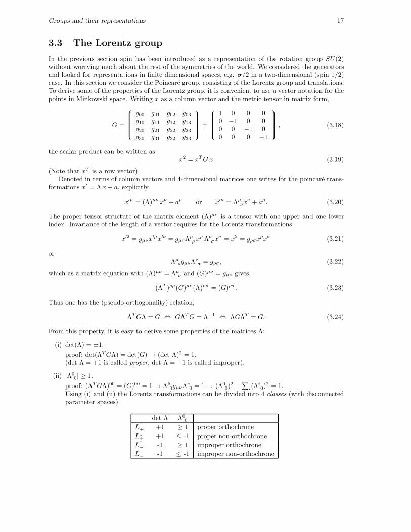
det Λ Λ00
L↑+ +1 ≥ 1 proper orthochrone
L↓+ +1 ≤ -1 proper non-orthochrone
L↑− -1 ≥ 1 improper orthochrone
L↓− -1 ≤ -1 improper non-orthochrone
Groups and their representations 18
(iii)∑3
i=1(Λi0)
2 =∑3
i=1(Λ0i )
2.
proof: use ΛTGΛ = G and ΛGΛT = G.
Note that Lorentz transformations generated from the identity must belong to L↑+, since I ∈ L↑+ and
det Λ and Λ00 change continuously along a path from the identity. In L↑+, one distinguishes rotations
and boosts. Rotations around the z-axis are given by ΛR(θ, z) = exp(i θ J3), infinitesimally given byΛR(θ, z) ≈ I + i θ J3. Thus
V 0′
V 1′
V 2′
V 3′
=
1 0 0 00 cos θ sin θ 00 − sin θ cos θ 00 0 0 1
V 0
V 1
V 2
V 3
−→ J3 =
0 0 0 00 0 −i 00 i 0 00 0 0 0
. (3.25)
Boosts along the z-direction are given by ΛB(φ, z) = exp(−i φK3), infinitesimally given by ΛB(φ, z) ≈I − i φK3. Thus
V 0′
V 1′
V 2′
V 3′
=
coshφ 0 0 sinhφ0 1 0 00 0 1 0
sinhφ 0 0 coshφ
V 0
V 1
V 2
V 3
−→ K3 =
0 0 0 i0 0 0 00 0 0 0i 0 0 0
. (3.26)
The parameter φ runs from −∞ < φ < ∞. Note that the velocity β = v = v/c and the Lorentzcontraction factor γ = (1 − β2)−1/2 corresponding to the boost are related to φ as γ = coshφ,βγ = sinhφ. Using these explicit transformations, we have found the generators of rotations, J =(J1, J2, J3), and those of the boosts, K = (K1,K2,K3), which satisfy the commutation relations(check!)
[J i, Jj ] = i ǫijk Jk,
[J i,Kj] = i ǫijk Kk,
[Ki,Kj ] = −i ǫijk Jk.
The first two sets of commutation relations exhibit the rotational behavior of J and K as vectors underrotations. From the commutation relations one sees that the boosts (pure Lorentz transformations)do not form a group, since the generators K do not form a closed algebra. the commutator of twoboosts in different directions (e.g. the difference of first performing a boost in the y-direction andthereafter in the x-direction and the boosts in reversed order) contains a rotation (in the examplearound the z-axis). This is the origin of the Thomas precession.
Returning to the global group, it is easy to find the following typical examples from each of thefour classes,
I =
+1 0 0 00 +1 0 00 0 +1 00 0 0 +1
∈ L↑+ (identity) (3.27)
It =
−1 0 0 00 +1 0 00 0 +1 00 0 0 +1
∈ L↓− (time inversion) (3.28)
Is =
+1 0 0 00 −1 0 00 0 −1 00 0 0 −1
∈ L↑− (space inversion) (3.29)
Groups and their representations 19
IsIt =
−1 0 0 00 −1 0 00 0 −1 00 0 0 −1
∈ L↓+ (space-time inversion) (3.30)
These four transformations form the Vierer group (group of Klein). Multiplying the proper or-thochrone transformations with one of them gives all Lorentz transformations.
Summarizing, the Lorentz transformations form a (Lie) group (Λ1Λ2 and Λ−1 are again Lorentz
transformations. There are six generators. Of the four parts only L↑+ forms a group. This is anormal subgroup and the factor group is the Vierer group. The extension to the Poincare group isstraightforward. Also this group can be divided into four parts, P ↑+ etc.
3.4 The generators of the Poincare group
The transformations belonging to P ↑+ are denoted as (Λ, a), infinitesimally approximated by (I+ω, ǫ),explicitly reading
x′µ = (Λ)µνxν + aµ inf= (δµν + (ω)µν)xν + ǫµ (3.31)
= Λµνx
ν + aµ = (gµν + ωµ
ν) xν + ǫµ.
The condition ΛTGΛ = G yields
(gρ
µ + ωρµ
)gρσ (gσ
ν + ωσν) = gµν =⇒ ωνµ + ωµν = 0, (3.32)
thus (ω)ij = −(ω)ji and (ω)0i = (ω)i0. We therefore find (again) that there are six generators for theLorentz group, three of which only involve spatial coordinates (rotations) and three others involvingtime components (boosts).
We now want to find a covariant form of the six generators of the Lorentz transformations, whichare obtained by writing the infinitesimal parameters (ω)µν in terms of six antisymmetric matrices(Mαβ)µν . One can easily convince oneself that
(ω)µν = ωµν = − i
2ωαβ (Mαβ)µν , (3.33)
(Mαβ)µν = i(gαµgβ
ν − gανg
βµ)
(3.34)
The algebra of the generators of the Lorentz transformations can be obtained by an explicit calcula-tion1,
[Mµν ,Mρσ] = −i (gµρMνσ − gνρMµσ) − i (gµσMρν − gνσMρµ) . (3.35)
Explicitly, we have for the (infinitesimal) rotations (around z-axis)
ΛR = I + i θ3 J3 = I − i ω12M12, (3.36)
with θi = − 12 ǫ
ijkωjk and J i = 12ǫ
ijkM jk (e.g. J3 = M12) and for the (infinitesimal) boosts (alongz-axis),
ΛB = I − i φ3K3 = I − i ω30M30, (3.37)
with φi = ωi0 and Ki = M0i (e.g. K3 = M03). Thus the two vector operators J and K form underLorentz transformations an antisymmetric tensor Mµν .
In order to find the commutation relations including the translation generators, we continue usingcovariance arguments. We will just require Poincare invariance for the generators themselves. The
1These commutation relations are the same as those for the ’quantummechanics’ operators i(xµ∂ν − xν∂µ)

Groups and their representations 20
infinitesimal form of any representation of the Poincare group (thus including the translations) is ofthe form
U(I + ω, ǫ) = 1 − i
2ωαβ M
αβ + i ǫα Pα. (3.38)
At this point, the generatorsMαβ no longer exclusively act in Minkowski space. The generators of thetranslations are the (momentum) operators Pµ. The requirement that Pµ transforms as a four-vector(for which we know the explicit behavior from the defining four-dimensional representation), leads to
U(Λ, a)PµU †(Λ, a) = (Λ)µνP
ν or U †(Λ, a)PµU(Λ, a) = (Λ−1)µνP
ν , (3.39)
(to decide on where the inverse is, check that U1U2 corresponds with Λ1Λ2). Infinitesimally,
(1 + iǫγPγ − i
2ωαβM
αβ)Pµ(1 − iǫδPδ +
i
2ωρσM
ρσ) = Pµ + ωµνP
ν , (3.40)
giving the following commutation relations by equating the coefficients of ǫµ and ωµν ,
[Pµ, P ν ] = 0, (3.41)
[Mµν , P ρ] = −i (gµρP ν − gνρPµ) . (3.42)
Note that the commutation relations among the generators Mµν in Eq. 3.35 could have been obtainedin the same way. They just state that Mµν transforms as a tensor with two Lorentz indices. Explicitly,writing the generator P = (H/c,P ) in terms of the Hamiltonian and the three-momentum operators,the tensor Mµν in terms of boosts cKi = M0i and rotations J i = 1
2 ǫijkM jk, one obtains
[P i, P j ] = [P i, H ] = [J i, H ] = 0, (3.43)
[J i, Jj ] = i ǫijkJk, [J i, P j] = i ǫijkP k, [J i,Kj] = i ǫijkKk, (3.44)
[Ki, H ] = i P i, [Ki,Kj] = −i ǫijkJk/c2, [Ki, P j] = i δijH/c2. (3.45)
We have here reinstated c, because one then sees that by letting c→ ∞ the commutation relations ofthe Galilei group, known from non-relativistic quantum mechanics are obtained.
3.5 Representations of the Poincare group
In order to label the states in an irreducible representation we construct a maximal set of commutingoperators. These define states with specified quantum numbers that are eigenvalues of these genera-tors. For instance, the generators J2 and J3 in the case of the rotation group. Taking any one of thestates in an irreducible representation, other states in that representation are obtained by the actionof operators outside the maximal commuting set. For instance, the generators J± in the case of therotation group.
Of the generators of the Poincare group we choose first of all the generators Pµ, that commuteamong themselves, as part of the set. The eigenvalues of these will be the four-momentum pµ of thestate,
Pµ|p, . . .〉 = pµ|p, . . .〉, (3.46)
where pµ is a set of four arbitrary real numbers. To find other generators that commute with Pµ welook for Lorentz transformations that leave the four vector pµ invariant. These form a group calledthe little group associated with that four vector.
Λµνp
ν = pµ + ωµνp
ν = pµ
⇒ ωµνpν = 0
⇒ ωµν = ǫµνρσpρsσ, (3.47)

Groups and their representations 21
where s is an arbitrary vector of which the length and the component along pσ are irrelevant, whichcan thus be chosen spacelike. The elements of the little group thus are
U(Λ(p)) = exp
(
− i
2ωµνM
µν
)
= exp
(
− i
2ǫµνρσM
µνpρsσ
)
(3.48)
and
U(Λ(p))|p, . . .〉 = exp
(
− i
2ǫµνρσM
µνpρsσ
)
|p, . . .〉 (3.49)
= exp (−isµWµ) |p, . . .〉 (3.50)
where the Pauli-Lubanski operators Wµ are given by
Wµ = −1
2ǫµνρσM
νρP σ. (3.51)
The following properties follow from the fact that Wµ is a four-vector by construction, of which thecomponents generate the little group of pµ or (for the third of the following relations) from explicitcalculation
[Mµν ,Wα] = −i (gµαWν − gναWµ) , (3.52)
[Wµ, Pν ] = 0, (3.53)
[Wµ,Wν ] = i ǫµνρσWρP σ. (3.54)
This will enable us to pick a suitable commuting ’spin’ operator. From the algebra of the generatorsone finds that
P 2 = PµPµ and W 2 = WµW
µ (3.55)
commute with all generators and therefore are invariants under Poincare transformations. Theseoperators are the Casimir operators of the algebra and can be used to define the representations ofP ↑+, for which we distinguish the following cases
p2 = m2 > 0 p0 > 0p2 = 0 p0 > 0pµ ≡ 0p2 = m2 > 0 p0 < 0p2 = 0 p0 < 0p2 < 0
Only the first two cases correspond to physical states, the third case represents the vacuum, while theothers have no physical significance.
Massive particles: p2 = M2 > 0, p0 > 0.
Given the momentum four vector pµ we choose a tetrade consisting of three orthogonal spacelike unitvectors ni(p), satisfying
gµνnµi (p)nν
j (p) = −δij , (3.56)
nµi (p) pµ = 0, (3.57)
ǫµνρσpµnν
i nρjn
σk = M ǫijk. (3.58)
Groups and their representations 22
We can write
Wµ(p) =
3∑
i=1
W i(p)nµi (p) (3.59)
(i.e. W i(p) = −W · ni(p)).Having made a covariant decomposition, it is sufficient to choose a particular frame to investigate
the coefficients in Eq. 3.59 The best insight in the meaning of the operators Wµ is to sit in the restframe of the particle and put Pµ = (M,0). In that case the vectors ni(p) are just the space directionsand W = (0,MJ) with components W i = (M/2)ǫijkM jk. The commutation relations
[W i(p),W j(p)] = iM ǫijkW k(p), (3.60)
show that W /M can be interpreted as the intrinsic spin.
More generally (fully covariantly) one can proceed by defining Si(p) ≡W i(p)/M and obtain
[Si(p), Sj(p)] = −inµi (p)nν
j (p)
M2ǫµνρσW
ρP σ = i ǫijkSk(p), (3.61)
i.e. the Si(p) form the generators of an SU(2) subgroup that belongs to the maximal set ofcommuting operators. Noting that
X
i
“
Si(p)”2
=1
M2W µ(p)W ν(p)
X
i
niµ(p)niν(p), (3.62)
and using the completeness relation
X
i
nµi (p)nν
i (p) = −„
gµν − pµpν
M2
«
, (3.63)
one sees thatX
i
“
Si(p)”2
= −W2
M2. (3.64)
Thus W 2 has the eigenvalues −M2 s(s + 1) with s = 0, 12 , 1, . . .. Together with the four momentum
states thus can be labeled as|M, s; p,ms〉, (3.65)
where E =√
p2 +M2 and ms is the z-component of the spin −s ≤ ms ≤ +s (in steps of one).The explicit construction of the wave function can be done using the D-functions (analogous as
the rotation functions). We will not do this but construct them as solutions of a wave equation to bediscussed explicitly in section 4
Massless particles: p2 = M2 = 0, p0 > 0.
In this case a set of four independent vectors is chosen starting with a reference frame in which pµ = pµ0
in the following way:
p0 = (p0, 0, 0, |p3|), (3.66)
n1(p0) ≡ (0, 1, 0, 0), (3.67)
n2(p0) ≡ (0, 0, 1, 0), (3.68)
s(p0) ≡ (1, 0, 0,−1) (3.69)
such that in an arbitrary frame where the four vectors p, n1(p), n2(p) and s(p) are obtained by aLorentz boost from the reference frame one has the property
ǫµνρσsµnν
1nρ2p
σ > 0. (3.70)
Groups and their representations 23
The above does actually include the massive case. The vector Wµ(p) now can be expanded
Wµ(p) = W 1(p)nµ1 (p) +W 2(p)nµ
2 (p) + λ(p) pµ +W s(p) sµ(p), (3.71)
where W · p = 0 implies that W s(p) = −(M2/p · s)λ(p). The algebra of W 1, W 2 and λ is derivedfrom the general commutation relations for [Wµ,Wν ], and gives
[W 1(p),W 2(p)] = iM2 λ(p), (3.72)
[λ(p),W 1(p)] = iW 2(p), (3.73)
[λ(p),W 2(p)] = −iW 1(p). (3.74)
We reproduce the algebra for the massive case with W 3(p) = M λ(p). But if M = 0 one has adifferent algebra (Eq. 3.72 has a vanishing right hand side). This algebra is (for instance) isomorphicto the one generated by rotations and translations in a 2-dimensional Euclidean plane (see exercises).The eigenvalues of W 1 and W 2 (in that case corresponding to the translations) thus can take anycontinuous values, implying continuous values for the spin (actually for W i = M Si). We don’t knowof any physical relevance, however, and the eigenvalues of W 1 and W 2 are set to zero (correspondingto the limit M → 0 for the WµWµ eigenvalues of M2 s(s+ 1) → 0). Thus we have
P 2, Pµ, Wµ(p) = λ(p)Pµ, W 2 (3.75)
as a commuting set with zero eigenvalues for P 2 and W 2. The meaning of λ(p) is most easily seen bycomparing for a momentum eigenstate
W 0(p) = λ(p) |p|
with
W 0(p) = −1
2ǫ0ijkMijpk = J · p.
Thus
λ(p) =J · p|p| , (3.76)
which is called the helicity. Note that angular momentum does not contribute to helicity as L ·p = 0.A massless particle, thus, is characterized by its momentum and the helicity,
|p, λ〉, (3.77)
which can take any integer or half-integer value.
The vacuum: pµ = 0.
This state is in physical applications nondegenerate and is denoted by
|0〉. (3.78)
One has Pµ|0〉 = Wµ|0〉 = 0 and the state is invariant under Lorentz transformations, U(Λ, a)|0〉 = |0〉.
Exercises
Exercise 3.1
Show that for a unitary operator U = exp[iαkJk] with real coefficients αk, the operators Jk mustbe hermitean. Show that if det(U) = 1, the trace of the operator Jk is zero (Convince yourself thatdet(eA) = eTrA by diagonalizing A; note that the definition of eA is eA ≡ ∑∞n=0A
n/n!).
Groups and their representations 24
Exercise 3.2
(a) Derive from the relation (valid for any vector a)
A(σ · a)A−1 = σ · RAa,
where A = exp(iφ · σ/2) = exp(iφσ · n/2), the relation
b · RAa = b · a cosφ+ n · (b × a) sinφ+ 2(b · n)(a · n) sin2(φ/2)
= b · a + b · (a × n) sinφ− 2 (b · a − (b · n)(a · n)) sin2(φ/2)
for any vectors a and b.
Note: Recall (or derive) that the Pauli matrices σ satisfy
Tr(σiσj) = 2 δij,
Tr(σiσjσk) = 2i ǫijk,
Tr(σiσjσkσl) = 2 (δij δkl − δik δjl + δil δjk) .
(b) Use the result under (a) to derive the matrix elements of a rotation around the z-axis and showthat it indeed represents the SO(3) rotation RA = exp(i φLz) in which the Lz is one of the(defining) generators of SO(3).
Excercise 3.3
Show that the Lie-algebra representations J = σ/2 and J = −σ∗/2 are equivalent, i.e. show thatone matrix ǫ exist such that ǫ†σǫ = −σ∗.
Excercise 3.4
Consider rotations and translations in a plane (two-dimensional Euclidean space). Use a 3-dimensionalmatrix representation or consider the generators of rotations and translations in the space of functionson the (x-y) plane. From either of these, derive the commutation relations and show that the algebra isisomorphic to (i.e., there is a one to one mapping) the algebra in Eqs 3.72 to 3.74 of the Pauli-Lubanskioperators for massless particles.
Exercise 3.5 (optional)
One might wonder if it is actually possible to write down a set of operators that generate the Poincaretransformations, consistent with the (canonical) commutation relations of a quantum theory. This ispossible for a single particle. Do this by showing that the set of operators,
H =√
p2 c2 +m2 c4,
P = p,
J = r × p + s,
K =1
2c2(rH +Hr) − tp +
p × s
H +mc2.
satisfy the commutation relations of the Poincare group if the position, momentum and spin operatorssatisfy the canonical commutation relations, [ri, pj ] = iδij and [si, sj ] = iǫijk sk; the others vanish,[ri, rj ] = [pi, pj] = [ri, sj] = [pi, sj ] = 0.Hint: for the Hamiltonian, show first the operator identity [r, f(p)] = i∇pf(p); if you don’t want todo this in general, you might just check relations involving J or K by taking some (relevant) explicitcomponents.

Groups and their representations 25
Just a comment: extending this to more particles is a highly non-trivial procedure, but it can bedone, although the presence of an interaction term V (r1, r2) inevitably leads to interaction terms inthe boost operators. These do not matter in the non-relativistic limit (c → ∞), that’s why many-particle non-relativistic quantum mechanics is ’easy’.

Chapter 4
The Dirac equation
4.1 The Lorentz group and SL(2, C)
Instead of the generators J and K of the homogeneous Lorentz transformations we can use the(non-hermitean) combinations
A =1
2(J + iK), (4.1)
B =1
2(J − iK), (4.2)
which satisfy the commutation relations
[Ai, Aj ] = i ǫijkAk, (4.3)
[Bi, Bj ] = i ǫijkBk, (4.4)
[Ai, Bj ] = 0. (4.5)
This shows that the Lie algebra of the Lorentz group is identical to that of SU(2)⊗SU(2). This tellsus how to find the representations of the group. They will be labeled by two angular momenta corre-sponding to the A and B groups, respectively, (j, j′). Special cases are the following representations:
Type I : (j, 0) K = −iJ (B = 0), (4.6)
Type II : (0, j) K = iJ (A = 0). (4.7)
From the considerations above, it also follows directly that the Lorentz group is homeomorphicwith the group SL(2, C), similarly as the homeomorphism between SO(3) and SU(2). The groupSL(2, C) is the group of complex 2 × 2 matrices with determinant one. It is simply connected and
forms the covering group of L↑+. It is easy to see that these matrices can be written as a product of aunitary matrix U and a hermitean matrix H ,
M = exp
(i
2θ · σ ± 1
2φ · σ
)
=
U(θ)H(φ)
U(θ)H(φ), (4.8)
with φ = φn and θ = θn, where we restrict (for fixed n the parameters 0 ≤ θ ≤ 2π and 0 ≤φ < ∞). With this choice of parameter-spaces the plus and minus signs are actually relevant. Theyprecisely correspond to the two types of representations that we have seen before, becoming thedefining representations of SL(2, C):
Type I (denoted M): J =σ
2, K = −i σ
2, (4.9)
Type II (denoted M): J =σ
2, K = +i
σ
2, (4.10)
26
The Dirac equation 27
Let us investigate the defining (two-dimensional) representations of SL(2, C). One defines spinors ξand η transforming similarly under unitary rotations (U † = U−1, U ≡ (U †)−1 = U)
ξ → Uξ, η → Uη, (4.11)
U(θ) = exp(i θ · σ/2)
but differently under hermitean boosts (H† = H , H ≡ (H†)−1 = H−1), namely
ξ −→ Hξ, η → Hη, (4.12)
H(φ) = exp(φ · σ/2),
H(φ) = exp(−φ · σ/2).
A practical boost for the spinors is the one transforming from the rest frame to the frame withmomentum p. With E = Mγ = M cosh(φ) and p = Mβγn = M sinh(φ) n it is given by
H(p) = exp
(φ · σ
2
)
= cosh
(φ
2
)
+ σ · n sinh
(φ
2
)
=M + E + σ · p√
2M(E +M), (4.13)
Also useful is the relation H2(p) = σµpµ/M = (E + σ · p)/M .The sets of four operators defined by definitions
σµ ≡ (1,σ), σµ ≡ (1,−σ), (4.14)
satisfying Tr(σµ σν) = −2 gµν and Tr(σµ σν) = 2gµν = 2 δµν (the matrices, thus, are not covariant!)
can be used to establish the homeomorphism between L↑+ and SL(2, C). The following relations forrotations and boosts are useful,
U σµaµ U−1 = σµΛRaµ, H σµaµH
−1 = σµΛBaµ (4.15)
U σµaµ U−1
= σµΛRaµ, H σµaµH−1
= σµΛBaµ. (4.16)
Non-equivalence of M and M
One might wonder if type I and type II representations are not equivalent, i.e. if there does not exista unitary matrix S, such that M = SMS−1. In fact, there exists the matrix
ǫ = iσ2, (ǫ∗ = ǫ; ǫ−1 = ǫ† = ǫT = −ǫ), (4.17)
that can be used to relate σµ∗ = ǫ†σµǫ = ǫ−1σµǫ and hence
U∗ = ǫ†Uǫ = ǫ† U ǫ, H∗ = ǫ†Hǫ = ǫ−1 Hǫ. (4.18)
As already discussed for SU(2), the first equation shows that the conjugate representation with spinorsχ∗ transforming according to −σ∗/2 is equivalent with the ordinary two-dimensional representation(±ǫχ∗ transforms according to σ/2). This is not true for the two-component spinors in SL(2, C) or
L↑+. Eqs 4.18 show that ±ǫξ∗ transforms as a type-II (η) spinor, while ±ǫη∗ transforms as a type-I
spinor. This shows that M∗ ≃M .Note that M∗ = ǫ†Mǫ has its equivalent for the Lorentz transformations Λ(M) and Λ(M∗).
They are connected via Λ(M∗) = Λ−1(ǫ)Λ(M)Λ(ǫ) within L↑+ because iσ2 = U(πy) showing that
ǫ ∈ SL(2, C) and, thus, Λ(ǫ) ∈ L↑+. The Lorentz transformations Λ(M) and Λ(M∗), however, cannot
be connected by a Lorentz transformation belonging to L↑+. One has
Λ(M∗) = I2 Λ(M) I−12 , (4.19)

The Dirac equation 28
where
I2 =
1 0 0 00 1 0 00 0 −1 00 0 0 1
. (4.20)
The matrix I2 does not belong to L↑+, but to L↑−. Thus M∗ and M are not equivalent within SL(2, C).
4.2 Spin 1/2 representations of the Lorentz group
Both representations (0, 12 ) and (1
2 , 0) of SL(2, C) are suitable for representing spin 1/2 particles. Theangular momentum operators J i are represented by σi/2, that have the correct commutation relations.Although these operators cannot be used to label the representations, but rather the operators W i(p)should be used, we have seen that in the rest frame W i(p)/M → J i, and the angular momentumin the rest frame is what we are familiar with as the spin of a particle. We also have seen thatthe representations (0, 1
2 ) and (12 , 0) are inequivalent, i.e. they cannot be connected by a unitary
transformation. Within the Lorentz group, they can be connected, but by a transformation belongingto the class P ↑−, as we have seen in section 4.1. The representing member of the class P ↑− is the parityor space inversion operator Is. A parity transformation changes aµ into aµ, where a = (a0,a) anda = (a0,−a). It has the same effect as lowering the indices. This provides the easiest way of seeingwhat is happening, e.g. ǫµνρσ will change sign, the aij elements of a tensor will not change sign.Examples (with between brackets the Euclidean assigments) are
r −→ −r (vector),
t −→ t (scalar),
p −→ −p (vector),
H −→ H (scalar),
J −→ J (axial vector),
λ(p) −→ −λ(p) (pseudoscalar),
K −→ −K (vector).
The behavior is the same for classical quantities, generators, etc. From the definition of the represen-tations (0, 1
2 ) and (12 , 0) (via operators J and K) one sees that under parity
(0,1
2) −→ (
1
2, 0). (4.21)
In nature parity turns (often) out to be a good quantum number for elementary particle states. For thespin 1/2 representations of the Poincare group including parity we, therefore, must combine the rep-resentations, i.e. consider the four component spinor that transforms under a Lorentz transformationas
u =
ξη
−→
M(Λ) 0
0 M(Λ)
ξη
, (4.22)
where M(Λ) = ǫM∗(Λ)ǫ−1 with ǫ given in Eq. 4.17. For a particle at rest only angular momentumis important and we can choose ξ(0,m) = η(0,m) = χm, the well-known two-component spinor for aspin 1/2 particle. Taking M(Λ) = H(p), the boost in Eq. 4.13, we obtain for the two components ofu which we will refer to as chiral right and chiral left components,
u(p,m) =
uR
uL
=
H(p) 0
0 H(p)
χm
χm
, (4.23)
The Dirac equation 29
with
H(p) =E +M + σ · p√
2M(E +M), (4.24)
H(p) =E +M − σ · p√
2M(E +M)= H−1(p). (4.25)
It is straightforward to eliminate χm and obtain the following constraint on the components of u,
0 H2(p)
H−2(p) 0
uR
uL
=
uR
uL
, (4.26)
or explicitly in the socalled Weyl representation
−M E + σ · p
E − σ · p −M
uR
uL
= 0, , (4.27)
which is an explicit realization of the (momentum space) Dirac equation, which in general is a linearequation in pµ,
(pµγµ −M)u(p) ≡ (/p−M)u(p) = 0, (4.28)
where γµ are 4 × 4 matrices called the Dirac matrices.As in section 2 we can use pµ = i∂µ to get the Dirac equation for ψ(x) = u(p)e−i p·x in coordinate
space,(iγµ∂µ −M)ψ(x) = 0, (4.29)
which is a covariant (linear) first order differential equation.The general requirements for the γ matrices are easily obtained. Applying (iγµ∂µ +M) from the
left gives(γµγν∂µ∂ν +M2
)ψ(x) = 0. (4.30)
Since ∂µ∂ν is symmetric, this can be rewritten
(1
2γµ, γν ∂µ∂ν +M2
)
ψ(x) = 0. (4.31)
To achieve also that the energy-momentum relation p2 = M2 is satisfied for u(p), one must requirethat for ψ(x) the Klein-Gordon relation
(2 +M2
)ψ(x) = 0 is valid for each component separately).
From this one obtains the Clifford algebra for the Dirac matrices,
γµ, γν = 2 gµν , (4.32)
suppressing on the RHS the identity matrix in Dirac space. The explicit realization appearing inEq. 4.27 is known as the Weyl representation. We will discuss another explicit realization of thisalgebra in the next section.
We first want to investigate if the Dirac equation solves the problem with the negative densitiesand negative energies. The first indeed is solved. To see this consider the equation for the hermiteanconjugate spinor ψ† (noting that γ†0 = γ0 and γ†i = −γi),
ψ†(
−iγ0←∂ 0 + iγi
←∂ i −M
)
= 0. (4.33)
Multiplying with γ0 on the right and pulling it through one finds
ψ(x)
(
iγµ←∂µ +M
)
= 0, (4.34)
The Dirac equation 30
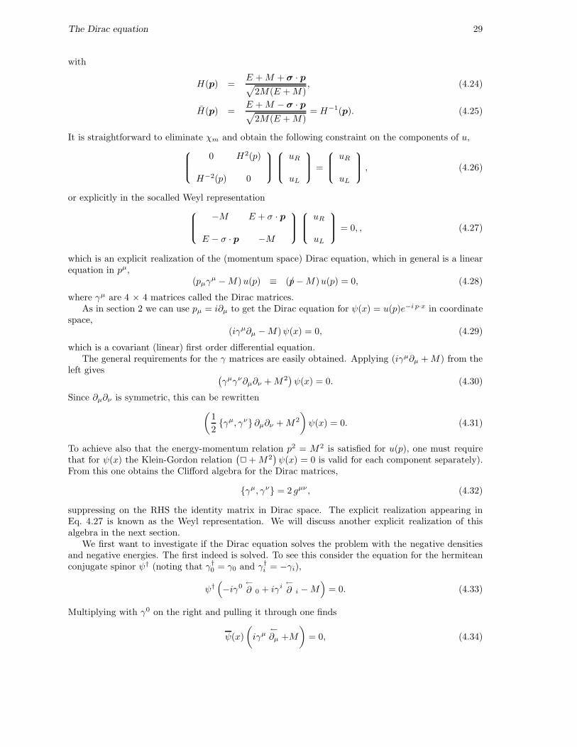
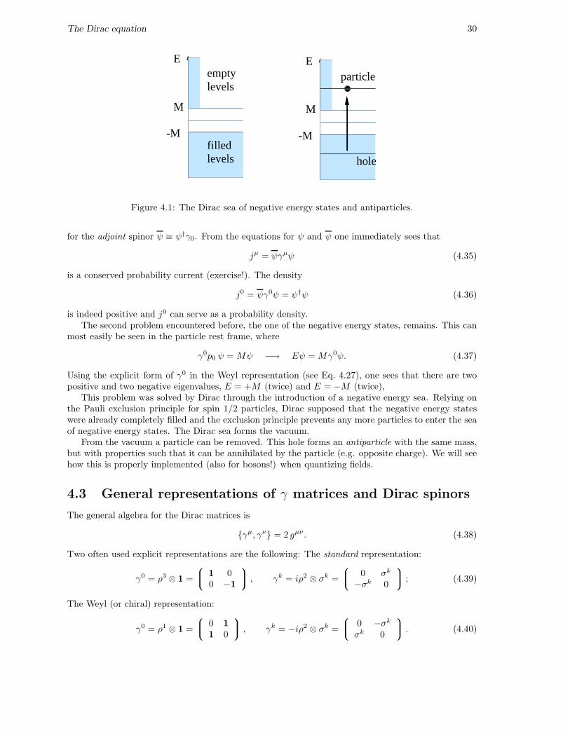
-M
M
E
filledlevels
emptylevels
-M
M
Eparticle
hole
Figure 4.1: The Dirac sea of negative energy states and antiparticles.
for the adjoint spinor ψ ≡ ψ†γ0. From the equations for ψ and ψ one immediately sees that
jµ = ψγµψ (4.35)
is a conserved probability current (exercise!). The density
j0 = ψγ0ψ = ψ†ψ (4.36)
is indeed positive and j0 can serve as a probability density.The second problem encountered before, the one of the negative energy states, remains. This can
most easily be seen in the particle rest frame, where
γ0p0 ψ = Mψ −→ Eψ = Mγ0ψ. (4.37)
Using the explicit form of γ0 in the Weyl representation (see Eq. 4.27), one sees that there are twopositive and two negative eigenvalues, E = +M (twice) and E = −M (twice),
This problem was solved by Dirac through the introduction of a negative energy sea. Relying onthe Pauli exclusion principle for spin 1/2 particles, Dirac supposed that the negative energy stateswere already completely filled and the exclusion principle prevents any more particles to enter the seaof negative energy states. The Dirac sea forms the vacuum.
From the vacuum a particle can be removed. This hole forms an antiparticle with the same mass,but with properties such that it can be annihilated by the particle (e.g. opposite charge). We will seehow this is properly implemented (also for bosons!) when quantizing fields.
4.3 General representations of γ matrices and Dirac spinors
The general algebra for the Dirac matrices is
γµ, γν = 2 gµν . (4.38)
Two often used explicit representations are the following: The standard representation:
γ0 = ρ3 ⊗ 1 =
1 00 −1
, γk = iρ2 ⊗ σk =
0 σk
−σk 0
; (4.39)
The Weyl (or chiral) representation:
γ0 = ρ1 ⊗ 1 =
0 1
1 0
, γk = −iρ2 ⊗ σk =
0 −σk
σk 0
. (4.40)
The Dirac equation 31
Different representations can be related to each other by unitary transformations,
γµ −→ SγµS−1, (4.41)
ψ −→ Sψ. (4.42)
We note that the explicit matrix taking us from the Weyl representation to the standard representation,(γµ)S.R. = S(γµ)W.R.S
−1, is
S =1√2
1 1
1 −1
. (4.43)
For all representations one hasㆵ = γ0γµγ0, (4.44)
and an adjoint spinor defined byψ = ψ†γ0. (4.45)
Another matrix which is often used is γ5 defined as
γ5 = i γ0γ1γ2γ3 = −i γ0γ1γ2γ3 =i ǫµνρσ
4!γµγνγργσ. (4.46)
It satisfies γ5, γµ = 0 and explicitly one has
(γ5)S.R. = ρ1 ⊗ 1 =
0 1
1 0
, (γ5)W.R. = ρ3 ⊗ 1 =
1 00 −1
. (4.47)
For instance in the Weyl representation (but valid generally), it is easy to see that
PR/L =1
2(1 ± γ5) (4.48)
are projection operators, that project out chiral right/left states, which in the case of the Weylrepresentation are just the upper and lower components.
Parity
There are a number of symmetries in the Dirac equation, e.g. parity. It is easy to convince oneselfthat if ψ(x) is a solution of the Dirac equation,
(i/∂ −M)ψ(x) = 0, (4.49)
one can apply space inversion, x = (t,x) → x = (t,−x) and via a few manipulations obtain again theDirac equation
(i/∂ −M)ψp(x) = 0, (4.50)
but with ψp(x) ≡ ηp γ0 ψ(x) (Exercise 4.5). Note that we have (as expected) explicitly in Weylrepresentation in Dirac space
ψ =
ξη
P−→ ψp = γ0 ψ =
ηξ
. (4.51)
Charge conjugation
The existence of positive and negative energy solutions implies another symmetry in the Dirac equa-tion. This symmetry does not change the spin 1/2 nature, but it does, for instance, reverse the chargeof the particle. As with parity we look for a transformation, called charge conjugation, that brings
The Dirac equation 32
ψ → ψc, which is again a solution of the Dirac equation. Starting with (i/∂ −M)ψ(x) = 0 we notethat by conjugating and transposing the Dirac equation one obtains
(iγµT∂µ +M
)ψ
T(x) = 0. (4.52)
In any representation a matrix C exist, such that
CγTµC−1 = −γµ, (4.53)
e.g.
(C)S.R. = iγ2γ0 = −iρ1 ⊗ σ2 =
0 −iσ2
−iσ2 0
=
0 −ǫ−ǫ 0
, (4.54)
(C)W.R. = iγ2γ0 = −iρ3 ⊗ σ2 =
−iσ2 0
0 iσ2
=
−ǫ 00 ǫ
. (4.55)
Thus we find back the Dirac equation,
(i/∂ −M)ψc(x) = 0. (4.56)
with the solutionψc(x) = ηc Cψ
T(x), (4.57)
where ηc is an arbitrary (unobservable) phase, usually to be taken unity. Some properties of C areC−1 = C† and CT = −C. One has ψc = −ψTC−1. In S.R. (or W.R.) and all representationsconnected via a real (up to an overall phase) matrix S, C is real and one has C−1 = C† = CT = −Cand [C, γ5] = 0. The latter implies that the conjugate of a right-handed spinor, ψ c
R, is a left-handedspinor. Explicitly, in Weyl representation we find in Dirac space
ψ =
ξη
C−→ ψc = C ψ
T=
−ǫ η∗ǫ ξ∗
. (4.58)
4.4 Plane wave solutions
For a free massive particle, the best representation to describe particles at rest is the standard repre-sentation, in which γ0 is diagonal (see discussion of negative energy states in section 4.1). The explicitDirac equation in the standard representation reads
i ∂∂t −M iσ · ∇
−iσ · ∇ −i ∂∂t −M
ψ(x) = 0. (4.59)
Looking for positive energy solutions ∝ exp(−iEt) one finds two solutions, ψ(x) = u±s(p) e−i p·x, with
E = Ep = +√
p2 +M2, where u satisfies
Ep −M −σ · p
σ · p −(Ep +M)
u(p) = 0, ⇔ (/p−M)u(p) = 0. (4.60)
There are also two negative energy solutions, ψ(x) = v±s(p) ei p·x, where v satisfies
−(Ep +M) σ · p
−σ · p (Ep −M)
v(p) = 0, ⇔ (/p+M) v(p) = 0. (4.61)

The Dirac equation 33
Explicit solutions in the standard representation are
u(p, s) =√
Ep +M
χs
σ·pEp+M χs
, v(p, s) =
√
Ep +M
σ·pEp+M χs
χs
, (4.62)
where χs are two independent (s = ±) two-component spinors.. Note that the spinors in the negativeenergy modes (antiparticles) could be two different spinors. Choosing χ = −ǫχ∗ (the equivalent spin1/2 conjugate representation), the spinors satisfy C uT (p, s) = v(p, s) and C vT (p, s) = u(p, s). Thesolutions are normalized to
u(p, s)u(p, s′) = 2M δss′ , v(p, s)v(p, s′) = −2M δss′ , (4.63)
u(p, s)v(p, s′) = v(p, s)u(p, s′) = 0, (4.64)
u†(p, s)u(p, s′) = v†(p, s)v(p, s′) = 2Ep δss′ . (4.65)
An arbitrary spin 1/2 field can be expanded in the independent solutions. After separating positiveand negative energy solutions as done in the case of the scalar field one has
ψ(x) =∑
s
∫d3k
(2π)3 2Ek
(u(k, s) e−i k·x b(k, s) + v(k, s) ei k·x d∗(k, s)
). (4.66)
It is straightforward to find projection operators for the positive and negative energy states
P+ =∑
s
u(p, s)u(p, s)
2M=
/p+M
2M, (4.67)
P− = −∑
s
v(p, s)v(p, s)
2M=
−/p+M
2M. (4.68)
In order to project out spin states, the spin polarization vector in the rest frame is the startingpoint. In that frame is a spacelike unit vector sµ = (0, s). In an arbitrary frame one has s · p = 0 ands(p) can e.g. be obtained by a Lorentz transformation. It is easy to check that
Ps =1 ± γ5/s
2=
1
2
1 ± σ · s 0
0 1 ∓ σ · s
(4.69)
(the last equality in the restframe and in standard representation) projects out spin ±1/2 states (checkthis in the restframe for s = z).
Note that for solutions of the massless Dirac equation /pψ = 0. Therefore, γ5/pψ = 0 but also /pγ5ψ= −γ5/pψ = 0. This means that in the solution space for massless fermions the chirality states,
ψR/L ≡ 1
2(I ± γ5)ψ, (4.70)
are independent solutions. In principle massless fermions can be described by two-component spinors.The chirality projection operators replace the spin projection operators which are not defined (by lackof a rest frame).
Explicit examples of spinors are useful to illustrate spin eigenstates, helicity states, chirality,etc. For instance with the z-axis as spin quantization axis, one has in standard representation:
u(p,+1/2) =1√
E +M
8
>
>
>
>
>
>
>
>
>
:
E +M0p3
p1 + i p2
9
>
>
>
>
>
>
>
>
>
;
, u(p,−1/2) =1√
E +M
8
>
>
>
>
>
>
>
>
>
:
0E +Mp1 − i p2
−p3
9
>
>
>
>
>
>
>
>
>
;
, (4.71)
The Dirac equation 34
v(p,+1/2) =1√
E +M
8
>
>
>
>
>
>
>
>
>
:
p1 − i p2
−p3
0E +M
9
>
>
>
>
>
>
>
>
>
;
, v(p,−1/2) =1√
E +M
8
>
>
>
>
>
>
>
>
>
:
−p3
−p1 − i p2
−(E +M)0
9
>
>
>
>
>
>
>
>
>
;
.
(4.72)Helicity states (p along z) in Standard representation are:
u(p, λ = +1/2) =
8
>
>
>
>
>
>
>
>
>
:
√E +M
0√E −M
0
9
>
>
>
>
>
>
>
>
>
;
, u(p, λ = −1/2) =
8
>
>
>
>
>
>
>
>
>
:
0√E +M
0
−√E −M
9
>
>
>
>
>
>
>
>
>
;
, (4.73)
v(p, λ = +1/2) =
8
>
>
>
>
>
>
>
>
>
:
0
−√E −M0√
E +M
9
>
>
>
>
>
>
>
>
>
;
, v(p, λ = −1/2) =
8
>
>
>
>
>
>
>
>
>
:
−√E −M0
−√E +M0
9
>
>
>
>
>
>
>
>
>
;
. (4.74)
By writing the helicity states in Weyl representation it is easy to project out righthanded (up-per components) and lefthanded (lower components). One finds for the helicity states in Weylrepresentation:
u(p, λ = +1/2) =1√2
8
>
>
>
>
>
>
>
>
>
:
√E +M +
√E −M
0√E +M −
√E −M
0
9
>
>
>
>
>
>
>
>
>
;
, u(p, λ = −1/2) =1√2
8
>
>
>
>
>
>
>
>
>
:
0√E +M −
√E −M
0√E +M +
√E −M
9
>
>
>
>
>
>
>
>
>
;
,
v(p, λ = +1/2) =1√2
8
>
>
>
>
>
>
>
>
>
:
0√E +M −
√E −M
0−√E +M −
√E −M
9
>
>
>
>
>
>
>
>
>
;
, v(p, λ = −1/2) =1√2
8
>
>
>
>
>
>
>
>
>
:
−√E +M −
√E −M
0+√E +M −
√E −M
0
9
>
>
>
>
>
>
>
>
>
;
.
Also for helicity states C uT (p, λ) = v(p, λ) and C uT (p, λ) = u(p, λ). We note that for high energythe positive helicity (λ = +1/2) is in essence righthanded, while the negative helicity (λ = −1/2)is in essence lefthanded. The ratio of the components is (directly or inversely) proportional to
√E +M −
√E −M√
E +M +√E −M
=2M
(√E +M +
√E −M)2
M≪E=⇒ M
2E,
which vanishes in the ultra-relativistic limit E ≫ M or in the massless case.
4.5 γ gymnastics and applications
An overview of properties can be found in many text books. Some elementary properties are:
Properties of products of γ-matrices:(1) γµγµ = 4(2) γµ γν γµ = −2 γν or γµ/aγµ = −2 /a.(3) γµ γργσ γµ = 4 gρσ or γµ/a/bγµ = 4 a · b.(4) γµ γνγργσ γµ = −2 γσγργν.(5) γµ γλγνγργσ γµ = 2
[γσγλγνγρ + γργνγλγσ
].
(6) γ5 = i γ0γ1γ2γ3 = −i ǫµνρσγµγνγργσ/4!.
(7) γµγ5 = -γ5γµ = i ǫµνρσγνγργσ/3!.
(8) σµν ≡ (i/2)[γµ, γν ](9) σµνγ5 = γ5σµν = ǫµνρσγ
ργσ/2.(10) γµγν = gµν − i σµν
(11) γµγνγρ = Sµνρσγσ + i ǫµνρσγσγ5 with Sµνρσ = (gµνgρσ - gµρgνσ + gµσgνρ).
The Dirac equation 35
Properties of traces of γ-matrices(1) Tr(γµ1 · · · γµn) = 0 if n is odd.(Use (γ5)
2 = 1 and pull one γ5 through.)(2) Tr(1) = 4.(3) Tr(γµγν) = 4 gµν or Tr(/a/b) = 4 a · b.(4) Tr(γµγνγργσ) = 4Sµνρσ.(5) Tr(γµ1 · · · γµn) = gµ1µ2Tr(γµ3 · · · γµn) - gµ1µ3Tr(γµ2γµ4 · · · γµn) + · · · .(6) Tr(γ5) = 0.(7) Tr(γ5γ
µγν) = 0 or Tr(γ5/a/b) = 0.(8) Tr(γ5γ
µγνγργσ) = −4i ǫµνρσ.(9) Tr(γµ1 · · · γµ2n) = Tr(γµ2n · · · γµ1).(Use matrices C to transpose the matrices in the expression under the trace and use TrAT = TrA.)
In order to show the use of the above relations, we will give one example, namely the calculationof the quantity
Lµν(k, k′) =1
2
∑
s,s′
(u(k, s)γµu(k′, s′))∗(u(k, s)γνu(k′, s′)) , (4.75)
which appears in quantum electrodynamics calculations (see Chapter 10) for the emission of a photonfrom an electron changing its momentum from k to k′ (k2 = k′2 = m2). In principle one can take arepresentation and just calculate the quantity u(k, s)γµu(k′, s′), etc. It is, however, more convenientto use the projection operators introduced earlier. For this we first have to prove (do this) that
(u(k, s)γµu(k′, s′))∗
= u(k′, s′)γµu(k, s), (4.76)
This leads with explicit Dirac indices to
Lµν =1
2
∑
s,s′
ui(k′, s′)(γµ)ijuj(k, s)uk(k, s)(γν)klul(k
′, s′)
=1
2
∑
s,s′
ul(k′, s′)ui(k
′, s′)(γµ)ijuj(k, s)uk(k, s)(γν)kl
=1
2(/k′ +m)li(γ
µ)ij(/k +m)jk(γν)kl
=1
2Tr [(/k′ +m)γµ(/k +m)γν ] .
The trace is linear and can be split up in parts containing traces with up to four gamma-matrices, ofwhich only the traces of four and two gamma-matrices are nonzero. They lead to
Lµν =1
2Tr [(/k′ +m)γµ(/k +m)γν ]
= 2[kµk′ν + kνk′µ − gµν(k · k′ −m2)
]
= 2 kµk′ν + 2 kνk′µ + (k − k′)2 gµν . (4.77)
Exercises
Excercise 4.1
Prove Eq. 4.13,
H(p) = exp
(φ · σ
2
)
=M + E + σ · p√
2M(E +M),
where E = Mγ = M cosh(φ) and p = Mβγn = M sinh(φ) n. Do this e.g. by proving
H2(p) = exp (φ · σ) = (E + σ · p)/M = σµpµ/M.
The Dirac equation 36
Exercise 4.2
Show that jµ = ψγµψ is a conserved current if ψ en ψ are solutions of the Dirac equation
Exercise 4.3
Show that in
P+ ≡∑
s=±1/2
u(p, s)u(p, s)
2M=
/p+M
2M
both sides are projection operators. Show that the equality holds, e.g. by letting them act on the fourbasis spinors u(p, s) and v(p, s).
Exercise 4.4
Show starting from the relation γµ, γν = 2gµν that
γµ/aγµ = −2 /a,
Tr(/a/b) = 4 a · b,Tr(γµ1 · · · γµn) = 0 if n is odd.
Excercise 4.5
Apply space-inversion, x → x, to the Dirac equation and use this to show that the spinor ψp(x) =γ0ψ(x), where x = (t,−x) is also a solution of the Dirac equation.
Exercise 4.6
(a) Show that (in standard representation)
ψ(x, t) = N
j0(kr)χm
i kE+M σ · r j1(kr)χm
e−i Et,
is a solution of the (free) Dirac equation. In this solution the wave number k = |k| =√E2 −M2
and χm a two-component spinor while j0 and j1 are spherical Bessel functions.
Note: use first the appropriate equation (which?) that is obeyed by each individual componentof the Dirac equation to show that the upper two components are allowed solutions.
(b) Next, we want to confine this solution to a spherical cavity with radius R. A condition forconfining the fermion in the cavity is i /nψ = ψ. Show that this condition is sufficient to guaranteethat nµj
µ = 0, i.e. there is no current flowing through the surface of the cavity.
Note: To prove this, you need to determine the corresponding confinement condition for ψ. Theconditions for ψ and ψ imply that nµj
µ = ψ/nψ = 0.
(c) Apply the confinement condition to find the lowest eigenmode in the spherical cavity for whichnµ = (0, r). Calculate it for MR = 0, MR = 1.5 and M → ∞.
(d) Plot for these cases the vector densities ψ†ψ and the scalar densities ψψ as a function of r/R.
Chapter 5
Maxwell equations
5.1 The electromagnetic field
With the electromagnetic field tensor
Fµν = ∂µAν − ∂νAµ (5.1)
=
0 −E1 −E2 −E3
E1 0 −B3 B2
E2 B3 0 −B1
E3 −B2 B1 0
, (5.2)
where Aµ is the four-vector potentialAµ = (φ,A), (5.3)
and the (conserved) current jµ = (ρ, j) the Maxwell equations read
∂µFµν = jν . (5.4)
Furthermore, the antisymmetry of Fµν implies that
∂µFµν = 0 or ∂λFµν + ∂µFνλ + ∂νFλµ = 0, (5.5)
where Fµν ≡ − 12ǫ
µνρσFρσ is the tensor where E → B and B → −E. It states the absence of magneticcharges and Faraday’s law.
For electrodynamics one has the freedom of gauge transformations. Under a gauge transformation
Aµ −→ Aµ + ∂µχ, (5.6)
the electric and magnetic fields are unchanged,
Fµν −→ Fµν + (∂µ∂νχ− ∂ν∂µχ) = Fµν . (5.7)
The equations of motion for the fields Aµ become
2Aµ − ∂µ(∂νAν) = jµ. (5.8)
This equation is not affected by a gauge transformation. The gauge freedom can be restricted byimposing the Lorenz condition
∂µAµ = 0, (5.9)
in which case one has2Aµ = jµ, (5.10)
37
Maxwell equations 38
of which the solutions give the Lienard-Wiechert potentials. The equation in vacuum, 2Aµ = 0,moreover, shows that the electromagnetic fields correspond to massless particles.
Although the Lorenz condition is a constraint, it does not eliminate the freedom of gauge trans-formations but they are now restricted to Aµ → Aµ + ∂µχ with 2χ = 0. The Lorenz condition canbe incorporated by changing the equations of motion to
2Aµ + (λ− 1)∂µ(∂νAν) = jµ. (5.11)
Taking the divergence one has for a conserved current and λ 6= 0 the condition
2∂µAµ = 0. (5.12)
Hence, if ∂µAµ = 0 for large times |t|, it will vanish at all times. This is not changed if in Eq. 5.11
the d’Alembertian is replaced by 2 +M2, corresponding to a massive field.The solutions of (2 +M2)Aµ = 0 are
Aµ(x) = ǫµ(k) e±ik·x. (5.13)
The Lorenz condition ∂µAµ = 0 implies that kµ ǫµ(k) = 0. In the restframe there are three independent
possibilities for ǫµ(k), namely (0, ǫλ), where the vectors ǫλ are the ones discussed in section 3.2,forming the basis for a spin 1 representation. The vectorfield is therefore suited to describe spin 1.
In an arbitrary frame ǫ(λ)µ (k) with λ = 0,±(1) are obtained by boosting the restframe vectors. The
(real) field Aµ(x), expanded in modes is given by
Aµ(x) =∑
λ=0,±
∫d3k
(2π)3 2E
(
ǫ(λ)µ (k) e−ik·x c(k, λ) + ǫ(λ)∗
µ (k) eik·x c∗(k, λ))
. (5.14)
Since the vectors ǫ(λ)µ (k) together with the momentum kµ form a complete set of four-vectors, one has
∑
λ=0,±ǫ(λ)µ (k) ǫ(λ)∗
ν (k) = −gµν +kµkν
M2. (5.15)
For M = 0, there is still a gauge freedom left (Aµ → Aµ + ∂µχ with 2χ = 0). One possible choiceis the gauge
A0 = 0 (5.16)
(radiation, transverse or Coulomb gauge). In that case one also has ∇·A = 0 or ki ǫi(k) = 0. Thereforeif kµ = (|k|, 0, 0, |k|), only two independent vectors remain
ǫ(±) µ(k) = (0,∓1,−i, 0), (5.17)
corresponding to the helicity states λ = ±1 of a massless photon.Note that via parity transformation one obtains another solution, AP
µ (x) = Aµ(x), while the fact
that the Minkowski space is real implies that ACµ (x) = A∗µ(x) = Aµ(x).
5.2 The electromagnetic field and topology∗
The electric and magnetic fields E and B as appearing for instance in the Lorentz force on a movingcharge,
F = eE + ev × B (5.18)
are gauge invariant, while the electromagnetic field Aµ is not. Nevertheless the significance of Aµ
is shown in the Aharonov-Bohm experiment. In this experiment an observable phase difference is
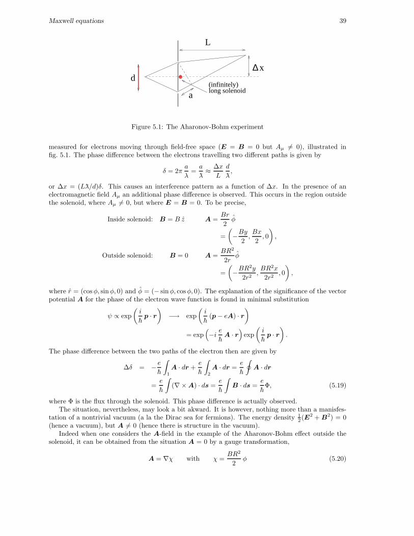
Maxwell equations 39
∆ x
L
a(infinitely)long solenoid
d
Figure 5.1: The Aharonov-Bohm experiment
measured for electrons moving through field-free space (E = B = 0 but Aµ 6= 0), illustrated infig. 5.1. The phase difference between the electrons travelling two different paths is given by
δ = 2πa
λ=a−λ≈ ∆x
L
d−λ,
or ∆x = (L−λ/d)δ. This causes an interference pattern as a function of ∆x. In the presence of anelectromagnetic field Aµ an additional phase difference is observed. This occurs in the region outsidethe solenoid, where Aµ 6= 0, but where E = B = 0. To be precise,
Inside solenoid: B = B z A =Br
2φ
=
(
−By2,Bx
2, 0
)
,
Outside solenoid: B = 0 A =BR2
2rφ
=
(
−BR2y
2r2,BR2x
2r2, 0
)
,
where r = (cosφ, sinφ, 0) and φ = (− sinφ, cosφ, 0). The explanation of the significance of the vectorpotential A for the phase of the electron wave function is found in minimal substitution
ψ ∝ exp
(i
hp · r
)
−→ exp
(i
h(p − eA) · r
)
= exp(
−i eh
A · r)
exp
(i
hp · r
)
.
The phase difference between the two paths of the electron then are given by
∆δ = − e
h
∫
1
A · dr +e
h
∫
2
A · dr =e
h
∮
A · dr
=e
h
∫
(∇× A) · ds =e
h
∫
B · ds =e
hΦ, (5.19)
where Φ is the flux through the solenoid. This phase difference is actually observed.The situation, nevertheless, may look a bit akward. It is however, nothing more than a manisfes-
tation of a nontrivial vacuum (a la the Dirac sea for fermions). The energy density 12 (E2 + B2) = 0
(hence a vacuum), but A 6= 0 (hence there is structure in the vacuum).Indeed when one considers the A-field in the example of the Aharonov-Bohm effect outside the
solenoid, it can be obtained from the situation A = 0 by a gauge transformation,
A = ∇χ with χ =BR2
2φ (5.20)

Maxwell equations 40
eiφ
Π1(S) = Z
U(1) S (space with solenoid)
class 0
class 1
class 2
Figure 5.2: The topology of the space in the Aharonov-Bohm experiment, illustrating also that thegroup structure of the mapping of U(1) into this space is that of the group of integers
(φ being the azimuthal angle). This situation that A can be written as ∇χ is always true when ∇×A
= 0. The observable phase going around in general is
∆δ =e
h
∮
A · dr =e
h
∮
∇χ · dr =e
hχ|φ=2π
φ=0 .
The function χ in Eq. 5.20, however, is multivalued as φ = 0 and φ = 2π are the same point in space.If this would be be happening in empty space one would be in trouble. By going around an arbitraryloop a different number of times the electron wave function would acquire different phases or it wouldacquire an arbitrary phase in a point by contracting a loop continuously into that point. Thereforethe gauge transformation must be uniquely defined in the space one is working in, implying that itmust be single-valued1.
Now back to the Aharonov-Bohm experiment. The difference here is that we are working ina space with a ’defect’ (the infinitely long solenoid). In such a space loops with different windingnumber (i.e. the number of times they go around the defect) cannot be continuously deformed intoone another. Therefore space outside the solenoid doesn’t care that χ is multi-valued. The Aharonov-Bohm experiment shows a realization of this possibility.
Another situation in which the topology of space can be used is in the case of superconductors.Consider a superconductor, forming a simple (connected) space. Below the critical temperature themagnetic field is squeezed out of the superconducting material, organizing itself in tiny flux tubes(Abrikosov strings), minimizing the space occupied by B fields. The only way for flux tubes to beformed and move around without global consequences is when each flux tube contains a flux Φ suchthat ∆δ = (e/h)Φ = n · 2π, giving no observable phase2.
1The occurrence of nontrivial possibilities, i.e. nonobservable phases φ = 2π n, has been employed by Dirac inconstructing magnetic monopoles in electrodynamics
2Actually, the relevant charge turns out to be 2e because the electrons appear in Cooper pairs
Maxwell equations 41
Exercises
Exercise 5.1
Show that Eqs. 5.4 and 5.5 explicitly give the equations
∇ · E = ρ,
∇ × B = j +∂E
∂t,
∇ × E +∂B
∂t= 0,
∇ · B = 0.
Chapter 6
Classical lagrangian field theory
6.1 Euler-Lagrange equations
In the previous chapter we have seen the equations for scalar fields (Klein-Gordon equation), Diracfields (Dirac equation) and massless vector fields (Maxwell equations) and corresponding to thesefields conserved currents describing the probability and probability current. These equations can beobtained from a lagrangian using the action principle.
As an example, recall classical mechanics with the action
S =
∫ t2
t1
dt L(x, x) (6.1)
and as an example the lagrangian
L(x, x) = K − V =1
2mx2 − V (x). (6.2)
The principle of minimal action looks for a stationary action under variations in the coordinates andtime, thus
t′ = t+ δτ, (6.3)
x′(t) = x(t) + δx(t), (6.4)
and the total changex′(t′) = x(t) + ∆x(t), (6.5)
with ∆x(t) = δx(t) + x(t) δτ . The requirement δS = 0 with fixed boundaries x(t1) = x1 and x(t2) =x2 leads to
δS =
∫ t2
t1
dt
∂L
∂xδx+
∂L
∂xδx
+ L δτ
∣∣∣∣
t2
t1
=
∫ t2
t1
dt
∂L
∂x− d
dt
(∂L
∂x
)
δx+
(∂L
∂xδx+ L δτ
)∣∣∣∣
t2
t1
. (6.6)
The first term leads to the Euler-Lagrange equations,
d
dt
(∂L
∂x
)
=∂L
∂x. (6.7)
The quantity ∂L/∂x plays a special role and is known as the canonical momentum,
p =∂L
∂x. (6.8)
42
Classical lagrangian field theory 43
For the lagrangian specified above this leads directly to Newton’s law p = mx = −∂V/∂x. The secondterm can be rewritten as
δS = . . .+
(∂L
∂x∆x−H δτ
)∣∣∣∣
t2
t1
, (6.9)
which is done because the first term (multiplying ∆x, which in classical mechanics vanishes at theboundary) does not play a role. The hamiltonian H is defined by
H(p, x) ≡ p x− L . (6.10)
One sees that invariance under time translations requires that H(t1) = H(t2), i.e. H is a conservedquantity.
In classical field theory one proceeds in complete analogy but using functions depending on spaceand time (classical fields, think for instance of a temperature or density distribution or of an electro-magnetic field). Consider a lagrangian density L which depends on these functions, their derivativesand possibly on the position, L (φ(x), ∂µφ(x), x) and an action
S[φ] =
∫ t2
t1
dt L =
∫
dt d3x L (φ(x), ∂µφ(x)) =
∫
R
d4x L (φ(x), ∂µφ(x)). (6.11)
Here R indicates a space-time volume bounded by (R3, t1) and R3, t2), also indicated by ∂R (amore general volume in four-dimensional space-time with some boundary ∂R can also be considered).Variations in the action can come from the coordinates or the fields, indicated as
x′µ = xµ + δxµ, (6.12)
φ′(x) = φ(x) + δφ(x) (6.13)
or combinedφ′(x′) = φ(x) + ∆φ(x), (6.14)
with∆φ(x) = δφ(x) + (∂µφ)δxµ. (6.15)
The resulting variation of the action is
δS =
∫
R
d4x′ L (φ′, ∂µφ′, x′) −
∫
R
d4x L (φ, ∂µφ, x). (6.16)
The change in variables x→ x′ in the integration volume involves a surface variation of the form∫
∂R
dσµ L δxµ.
Note for the specific choice of the surface for constant times t1 and t2,∫
∂R
dσµ . . . =
∫
(R3,t2)
d3x . . .−∫
(R3,t1)
d3x . . . . (6.17)
Furthermore the variations δφ and δ∂µφ contribute to δS, giving1
δS =
∫
R
d4x
[δL
δ(∂µφ)δ(∂µφ) +
δL
δφδφ
]
+
∫
∂R
dσµ L δxµ
=
∫
R
d4x
[δL
δφ− ∂µ
(δL
δ(∂µφ)
)]
δφ+
∫
∂R
dσµ
[δL
δ(∂µφ)δφ+ L δxµ
]
. (6.18)
1Taking a functional derivative, indicated with δF [φ]/δφ should pose no problems. We will come back to it in a bitmore formal way in section 9.2.
Classical lagrangian field theory 44
With for the situation of classical fields all variations of the fields and coordinates at the surfacevanishing, the second term is irrelevant. The integrand of the first term must vanish, leading to theEuler-Lagrange equations,
∂µ
(δL
δ(∂µφ)
)
=δL
δφ. (6.19)
6.2 Lagrangians for spin 0, 1/2 and 1 fields
By an appropriate choice of lagrangian density the equations of motion discussed in previous chaptersfor the scalar field (spin 0), the Dirac field (spin 1/2) and the vector field (spin 1) can be recovered,
The scalar field
It is straightforward to derive the equations of motion for a real scalar field φ from the followinglagrangian densities, which differ only by surface terms,
L =1
2∂µφ∂
µφ− 1
2M2 φ2 (6.20)
= −1
2φ(∂µ∂
µ +M2)φ, (6.21)
leading to(2 +M2)φ(x) = 0. (6.22)
For the complex scalar field one conventionally uses
L = ∂µφ∗∂µφ−M2 φ∗φ (6.23)
= −φ∗(∂µ∂
µ +M2)φ, (6.24)
which can be considered as the sum of the lagrangian densities for two scalar fields φ1 and φ2 with φ= (φ1 + iφ2)/
√2. One easily obtains
(2 +M2)φ(x) = 0, (6.25)
(2 +M2)φ∗(x) = 0. (6.26)
The Dirac field
The appropriate lagrangian from which to derive the equations of motion is
L =i
2ψ↔/∂ ψ −M ψψ =
i
2ψ→/∂ ψ − i
2ψ←/∂ ψ −M ψψ (6.27)
= ψ (i/∂ −M)ψ, (6.28)
where the second line is not symmetric but in the action only differs from the symmetric version bya surface term (partial integration). Using the variations in ψ (in the symmetric form),
δL
δ(∂µψ)= − i
2γµψ
δL
δψ=
i
2
→/∂ ψ −M ψ,
one obtains immediately(
i→/∂ −M
)
ψ = 0, (6.29)
Classical lagrangian field theory 45
and similarly from the variation with respect to ψ
ψ
(
i←/∂ +M
)
= 0. (6.30)
It is often useful to link to the two-component spinors ξ and η which we started with in chapter 4, orequivalently separate the field into right- and lefthanded ones. In that case one finds trivially
L =1
2ψR i
↔/∂ ψR +
1
2ψL i
↔/∂ ψL −M (ψR ψL + ψL ψR), (6.31)
showing e.g. that the lagrangian separates into two independent parts for M = 0.
The mass term in the Dirac lagrangian 6.31 rewritten in terms of ξ and η is
LM (Dirac) = −M“
ξ†η + η†ξ”
. (6.32)
There exists a different possibility to write down a mass term with only one kind of fields, namely2
LM (Majorana) = +1
2
“
M η†ǫη∗ −M∗ ηT ǫη”
. (6.33)
Since the kinetic term in L separates naturally in ξ and η, it is possible to introduce ’real’ spinorsor Majorana spinors that satisfies Υc = Υ. The spinor to be used satisfies
Υc = Υ and ΥL = ψL =
8
>
>
:
0η
9
>
>
;
⇒ Υ ≡8
>
>
:
−ǫ η∗η
9
>
>
;
, (6.34)
for which η0 = ǫ η∗0 . We note that
ψcL ≡ (ψL)c = C ψL
T=
8
>
>
:
−ǫ η∗0
9
>
>
;
= ΥR. (6.35)
Rewriting the Majorana mass term in Eq. 6.33 in terms of ψL and ψcL one finds
L =1
2ψL i
↔
/∂ ψL − 1
2
`
M ψcL ψL +M∗ ψL ψ
cL
´
. (6.36)
Note actually that using the following relations for Majorana spinors, ΥcR = ΥL and Υc
L = ΥR,the Majorana lagrangian is actually almost of the same form as the Dirac mass term,
L =1
4Υ i
↔
/∂ Υ − 1
2
`
M ΥRΥL +M∗ ΥLΥR
´
. (6.37)
Note the factor 1/2 as compared to the Dirac lagrangian, which comes because we in essence use’real’ spinors. The Majorana case is actually more general, since a lagrangian with both Dirac andMajorana mass terms can be rewritten as the sum of two Majorana lagrangians after redefiningthe fields (See e.g. Peshkin and Schroeder).
Vector field
From the lagrangian density
L = −1
4FµνF
µν +1
2M2 VµV
µ − λ
2(∂µV
µ)2
(6.38)
=1
2V µ[(∂2 +M2)gµν − (1 − λ)∂µ∂ν
]V ν , (6.39)
2This term is written down with η being an anticommuting Grassmann number for which
αβ = −βα,(αβ)∗ = β∗α∗ = −α∗β∗,
and thus (β∗α)∗ = α∗β = −βα∗. The reasons for Grassmann variables will become clear in the next chapter.
Classical lagrangian field theory 46
one immediately obtains
δL
δ(∂µVν)= −∂µV ν + ∂νV µ − λ gµν (∂ρV
ρ),
leading to the equations of motion
(2 +M2
)V µ − (1 − λ)∂µ(∂νV
ν) = 0, (6.40)
implying∂µF
µν +M2 V ν = 0 and ∂µVµ = 0. (6.41)
6.3 Symmetries and conserved (Noether) currents
For quantum fields (φ operator!) and in the case of the existence of symmetries variations at thesurface become important. In the first case it is not possible to specify for instance φ and φ on thesurface σ1. Also when the lagrangian is invariant under symmetries one can consider variations at theinitial or final surface that do not affect the dynamics. Returning to δS the surface term is rewrittento
δS =
∫
R
d4x . . .+
∫
∂R
dσµ
δL
δ(∂µφ)∆φ−
[δL
δ(∂µφ)∂νφ− L gµν
]
δxν
≡∫
R
d4x . . .+
∫
∂R
dσµ
δL
δ(∂µφ)∆φ− Θµν(x)δxν
, (6.42)
where
Θµν =δL
δ(∂µφ)∂νφ− L gµν . (6.43)
The variation δS thus can be expressed as
δS = F (σ1) − F (σ2) =
∫
∂R
dσµ Jµ(x) =
∫
R
d4x ∂µJµ(x), (6.44)
with
Jµ(x) = − δL
δ(∂µφ)∆φ+ Θµν(x)δxν . (6.45)
Thus considering ∂R = σ2 - σ1 with σ = (R3, t), the presence of a symmetry that leaves the lagrangianinvariant, requires the presence of a conserved quantity, F (t1) = F (t2), which is the space-integralover the zero-component of a conserved current, ∂µJ
µ(x) = 0,
F (t) =
∫
d3x J0(x, t), (6.46)
In the case of quantum fields, discussed in the next chapter, these conserved quantities becomeoperators, which in a consistent picture precisely generate the symmetries.
As an example consider U(1) transformations of the Dirac field proportional to the charge e,
ψ(x) → ei eΛψ(x) or ∆ψ(x) = i eΛψ(x). (6.47)
From the lagrangian for the Dirac field, we obtain (since δxµ = 0), omitting the parameter Λ
jµ = − δL
δ(∂µψi)· (−i e ψi
) − δL
δ(∂µψi)· (i e ψi)
= e ψγµψ. (6.48)
Classical lagrangian field theory 47
For the complex scalar field the U(1) transformations leave the lagrangian invariant and lead to theconserved current (see Exercise 6.3)
jµ = i e φ∗↔∂µ φ. (6.49)
These currents are conserved as discussed already in chapter 2. The integral over the zero-component,Q =
∫d3x j0(x, t) is the conserved charge (Q = 0). In the next section we will see the quantity show
up as the charge operator.
6.4 Space-time symmetries
One kind of symmetries that leave the lagrangian invariant are the Poincare transformations, includingthe space-time translations and the Lorentz transformations.
Translations
Under translations (generated by Pµop) we have
δxµ = ǫµ, (6.50)
∆φ(x) = 0, (6.51)
δφ(x) = −(∂µφ)δxµ = −ǫµ∂µφ(x). (6.52)
The behavior of the field under translations (δφ) is governed by the translational behavior of theargument in such a way that ∆φ = 0. From Noether’s theorem one sees that the current Θµνǫνis conserved. Therefore there are four conserved currents Θµν (ν labeling the currents!) and fourconserved quantities
P ν =
∫
dσµ Θµν =
∫
d3xΘ0ν . (6.53)
These are the energy and momentum. For quantized fields this will become the expressions of thehamiltonian and the momentum operators in terms of the fields, e.g. H =
∫d3xΘ00(x).
Lorentz transformations
In this case the transformation of the coordinates and fields are written as
δxµ = ωµνxν , (ωµνantisymmetric) (6.54)
∆φi(x) =1
2ωρσ(−i Sρσ)i
jφj(x). (6.55)
Note that the coordinate transformations can be written in a form similar to that for the fields,
δxµ =1
2ωρσ(aρσ)µ
νxν (6.56)
with(aρσ)µ
ν = gρµgσν − gσµgρ
ν . (6.57)
For the fields the behavior under Lorentz transformations has been the subject of chapter 3.Summarizing,
• Scalar field φ: −i Sρσ = 0.
• Dirac field ψ: −i Sρσ = −(1/4)[γρ, γσ]This result for the Dirac field is the same as discussed in chapter 3, but stated as the generalresult. Any specific behavior under Lorentz transformations may be found by substituting a
Classical lagrangian field theory 48
specific representation of the Dirac matrices. The general behavior (expressed in Dirac matrices)can be obtained by requiring them to behave as a four-vector, i.e. when ψ → Lψ with L =1 − (i/2)ωρσS
ρσ one has
L−1γµL = Λµνγ
ν with Λµν = gµ
ν + ωµν
[γµ, i Sρσ] = (aρσ)µνγ
ν = gρµγσ − gσµγρ,
−i Sρσ =1
4[γρ, γσ] = −i σ
ρσ
2.
• Vector field Aµ: −i Sρσ = aρσ.
The current following from Noether’s theorem is
Jµ = − δL
δ(∂µφi)∆φi + Θµνδxν
=1
2ωρσ
− δL
δ(∂µφi)(−i Sρσ)i
jφj + Θµρxσ − Θµσxρ
(6.58)
=1
2ωρσ Hµρσ + Θµρxσ − Θµσxρ (6.59)
=1
2ωρσM
µρσ. (6.60)
Therefore there are six conserved currentsMµρσ labeled by ρ and σ (antisymmetric) and correspondingto it there exist conserved quantities
Mρσ =
∫
d3x M0ρσ. (6.61)
A final note concernes the symmetry properties of Θµν . In general this tensor is not symmetric. Insome applications (specifically coupling to gravity) it is advantageous to have an equivalent currentthat is symmetric. Defining
Tµν = Θµν − ∂ρGρµν , (6.62)
with Gρµν = (Hρµν + Hµνρ + Hνµρ)/2, where Hρµν is the quantity appearing in Mρµν , one has atensor that satisfies
Tµν = T νµ, (6.63)
∂µTµν = ∂µΘµν , (6.64)
Mµρσ = Tµρxσ − Tµσxρ. (6.65)
6.5 (Abelian) gauge theories
In section 6.3 we have seen global transformations or gauge transformations of the first kind, e.g.
φ(x) → ei eΛφ(x), (6.66)
in which the U(1) transformation involves an angle eΛ, independent of x. Gauge transformations ofthe second kind or local gauge transformations are transformations of the type
φ(x) → ei eΛ(x)φ(x), (6.67)
i.e. the angle of the transformation depends on the space-time point x. The lagrangians which wehave considered sofar are invariant under global gauge transformations and corresponding to this there
Classical lagrangian field theory 49
exist a conserved Noether current. Any lagrangian containing derivatives, however, is not invariantunder local gauge transformations,
φ(x) → ei eΛ(x)φ(x), (6.68)
φ∗(x) → e−i eΛ(x)φ∗(x), (6.69)
∂µφ(x) → ei eΛ(x)∂µφ(x) + i e ∂µΛ(x) ei eΛ(x)φ(x), (6.70)
where the last term spoils gauge invariance.A solution is the one known as minimal substitution in which the derivative ∂µ is replaced by a
covariant derivative Dµ which satisfies
Dµφ(x) → ei eΛ(x)Dµφ(x). (6.71)
For this purpose it is necessary to introduce a vector field Aµ,
Dµφ(x) ≡ (∂µ + i eAµ(x))φ(x), (6.72)
The required transformation for Dµ then demands
Dµφ(x) = (∂µ + i eAµ(x))φ(x)
→ ei eΛ∂µφ+ i e (∂µΛ) ei eΛφ+ i eA′µ ei eΛφ
= ei eΛ(∂µ + i e(A′µ + ∂µΛ)
)φ
≡ ei eΛ (∂µ + i eAµ)φ. (6.73)
Thus the covariant derivative has the correct transformation behavior provided
Aµ → Aµ − ∂µΛ, (6.74)
the behavior which we have encountered before as a gauge freedom for massless vector fields withthe (free) lagrangian density L = −(1/4)FµνF
µν . Replacing derivatives by covariant derivatives andadding the (free) part for the massless vector fields to the original lagrangian therefore produces agauge invariant lagrangian,
L (φ, ∂µφ) =⇒ L (φ,Dµφ) − 1
4FµνF
µν . (6.75)
The field φ is used here in a general sense standing for any possible field. As an example consider theDirac lagrangian,
L =i
2
(ψγµ∂µψ − (∂µψ)γµψ
)−M ψψ.
Minimal substitution ∂µψ → (∂µ + i eAµ)ψ leads to the gauge invariant lagrangian
L =i
2ψ↔/∂ ψ −M ψψ − e ψγµψAµ − 1
4FµνF
µν . (6.76)
We note first of all that the coupling of the Dirac field (electron) to the vector field (photon) can bewritten in the familiar interaction form
Lint = −e ψγµψAµ = −e jµAµ, (6.77)
involving the interaction of the charge (ρ = j0) and three-current density (j) with the electric potential(φ = A0) and the vector potential (A), −e jµAµ = −e ρφ + e j · A. The equation of motion for thefermion follow from
δL
δ(∂µψ)= − i
2γµψ,
δL
δψ=
i
2/∂ψ −M ψ − e/Aψ
Classical lagrangian field theory 50
giving the Dirac equation in an electromagnetic field,
(i/D −M)ψ = (i/∂ − e/A−M)ψ = 0. (6.78)
For the photon the equations of motion follow from
δL
δ(∂µAν)= −Fµν ,
δL
δAν= −eψγνψ,
giving the Maxwell equation coupling to the electromagnetic current,
∂µFµν = jν , (6.79)
where jµ = e ψγµψ.
Exercises
Exercise 6.1
(a) Show that the Klein-Gordon equation for the real scalar field can be derived from the lagrangiandensity
L =1
2∂µφ∂
µφ− 1
2M2 φ2.
(b) Show that the Klein-Gordon equation for the complex scalar field (considering φ and φ∗ asindependent fields can be derived from the lagrangian density
L = ∂µφ∗∂µφ−M2 φ∗φ.
Exercise 6.2
(a) Show that the homogeneous Maxwell equations can be derived from the lagrangian density
L = −1
4FµνF
µν .
(b) What is the form of the interaction term involving a current jµ and the field Aµ that will givethe inhomogeneous Maxwell equations, ∂µF
µν = jν .
(c) Show that the interaction term is invariant under gauge transformations only if the current jµ isconserved, i.e. ∂µj
µ = 0 (Note that the addition of a total derivative to the lagrangian densitydoes not modify the equations of motion).
Exercise 6.3
Show that the current jµ = i φ∗↔∂µ φ for a complex scalar field is connected to a U(1) transformation
on the fields, φ → eiΛ φ.
Exercise 6.4
Given the Dirac equation for a (negatively charged) spin-1/2 particle in an external electromagnetic
field, [iγµ(∂µ − i eAµ)−M ]ψ = 0, give the equation which is satisfied by ψc = CψT, and deduce what
is the charge of the antiparticle as compared to a particle.
Classical lagrangian field theory 51
Exercise 6.5
Show that the Dirac equation for an electron with charge −e in an external electromagnetic field Aµ
= (A0,A) (see also exercise 6.4) for a stationary solution in the non-relativistic (and weak-field) limityields in the standard representation the following equation for the ’upper (two) components’ ψu,
(1
2M(−i∇ + eA)2 +
e
2Mσ · B − eA0
)
ψu(r, t) = En.r.ψu(r, t),
with En.r. = E −M .
Exercise 6.6 (optional)
Prove the properties of the tensor T µν in section 6.4.Hints: it may be useful to realize that Gµρσ is antisymmetric in first two indices; use ∂µT
µν = 0 and∂µM
µρσ = 0, in order to show that Θρσ −Θσρ = ∂µHµρσ; finally note that it is sufficient to show the
last equation for∫dσµM
µρσ.

Chapter 7
Quantization of fields
7.1 Canonical quantization
We will first recall the example of classical mechanics for one coordinate q(t), starting from thelagrangian L(q, q) also considered in the previous chapter,
L(q, q) =1
2mq2 − V (q). (7.1)
The Hamiltonian (also corresponding to a conserved quantity because of time translation invariance)is given by
H(p, q) = p q − L(q, q(q, p)) (7.2)
=p2
2m+ V (q), (7.3)
where the (canonical) momentum p = ∂L/∂q, in our example p = mq. Quantizing the system,canonical commutation relations between q and p are imposed,
[q, p] = i, (7.4)
with a possible realization as operators in the Hilbert space of (coordinate space) wave functionsthrough qopψ(q) = qψ(q) and popψ(q) = −idψ/dq.
An immediate generalization for fields can be obtained by considering them as coordinates, labeledby the position,
qx(t) =1
∆3x
∫
∆3x
d3x φ(x, t), (7.5)
etc. The lagrangian is given by
L =
∫
d3x L (φ(x), ∂µφ(x)) =
∫
d3x L (φ, φ,∇φ)
=∑
x
∆3xL x (qx, qx, qx+∆x) , (7.6)
In order to construct the hamiltonian it is necessary to find the canonical momenta,
px(t) =∂L
∂qx= ∆3x
∂Lx
∂qx= ∆3xΠx(t), (7.7)
52
Quantization of fields 53
where Πx(t) is obtained from the continuous field Π(x) ≡ δL /δ(∂0φ). The hamiltonian then is
H =∑
x
pxqx − L =∑
x
∆3x [Πxqx − L x] (7.8)
=∑
x
∆3xHx (7.9)
where
H (x) =δL
δφ(x)φ(x) − L (x) = Θ00(x). (7.10)
Note that this indeed corresponds to the zero-zero component (Θ00) of the conserved energy-momentumstress tensor Θµν , discussed in the section 6.2.
As an example, for the scalar field theory, we have
L (x) =1
2∂µφ∂
µφ− 1
2M2 φ2
=1
2(∂0φ)2 − 1
2(∇φ)2 − 1
2M2 φ2 (7.11)
Π(x) =δL
δ∂0φ)= ∂0φ, (7.12)
H (x) = Θ00(x) =1
2(∂0φ)2 +
1
2(∇φ)2 +
1
2M2 φ2. (7.13)
For the quantization procedure we can formulate a number of basic axioms of quantum field theory.Sometimes it is useful to keep in mind that, formally, the fields φ(x) can be considered as regularoperators in the Hilbert space after smearing with a test function f ,
Φ(f) =
∫
d4x φ(x) f(x). (7.14)
In fact, the discretization procedure above is an explicit example, albeit with ’sharp’ functions.The following items are essential for quantization of a theory.
• Canonical commutation relations
Quantization of the theory is achieved by imposing the canonical quantization condition [qx(t), py(t)]= i δxy or for the fields φ(x) and Π(x) the socalled equal time commutation relations
[φ(x, t),Π(y, t)] = i δ3(x − y), (7.15)
with furthermore the relations [φ(x, t), φ(y, t)] = [Π(x, t),Π(y, t)] = 0.
• Poincare invariance
The fields must satisfy the following transformation properties
U †(Λ, a)φi(x)U(Λ, a) = Rij(Λ−1)φj(Λ−1x− a), (7.16)
or if
U(Λ, a) = 1 + iǫµPµ − i
2ωµνM
µν ,
Rij(Λ−1) = 1 − i
2ωµν(Sµν)i
j ,
one has
[φi(x), Pµ] = i∂µφi(x), (7.17)
[φi(x),Mµν ] = i(xµ∂ν − xν∂µ)φi(x) + (Sµν)ijφ
j(x), (7.18)
with Sµν given in 6.4.2. This must be valid for the operator Pµ and Mµν expressed in terms ofthe fields via Noether’s theorem.
Quantization of fields 54
• Causality
Operators Φ(f) and Φ(g) for which the test functions are space-like separated can be mea-sured simultaneously (macroscopic causality). The measurements cannot influence each otheror [Φ(f),Φ(g)] = 0. Microscopic causality implies local commutativity,
[φ(x), φ(y)] = 0 if (x− y)2 < 0. (7.19)
7.2 Creation and annihilation operators
Before discussing (real and complex) scalar fields and Dirac fields we recall the analogy with the well-known harmonic oscillator as an example of quantization using creation and annihilation operators,sometimes referred to as second quantization. In simplified form the hamiltonian is given by
H =1
2P 2 +
1
2ω2Q2, (7.20)
where the coordinate Q and the momentum P satisfy the canonical commutation relations
[Q,P ] = i, [Q,Q] = [P, P ] = 0 (7.21)
Writing Q and P in terms of creation (a†) and annihilation (a) operators,
Q =1√2ω
(a+ a†) and P = −i√ω
2(a− a†) (7.22)
it is straightforward to check that the commutation relations between Q and P are equivalent withthe commutation relations
[a, a†] = 1, [a, a] = [a†, a†] = 0. (7.23)
The hamiltonian in this case can be expressed in the number operator N = a†a,
H = ω
(√ω
2Q− i
P√2ω
)(√ω
2Q+ i
P√2ω
)
− i
2[Q,P ]
= ω
a†a+1
2
= ω
N +1
2
. (7.24)
It is straightforward to find the commutation relations between N and a and a†,
[N, a†] = a†, and [N, a] = −a. (7.25)
Defining states |n〉 as eigenstates of N with eigenvalue n, N |n〉 = n|n〉 one finds
N a†|n〉 = (n+ 1) a†|n〉,N a|n〉 = (n− 1) a|n〉
i.e. a† and a act as raising and lowering operators. From the normalizations one obtains a†|n〉 =√n+ 1 |n + 1〉 and a|n〉 =
√n |n − 1〉, and we see that a state |0〉 must exist for which N |0〉 = a|0〉
= 0. In this way one has found for the harmonic oscillator the spectrum of eigenstates |n〉 (with n anon-negative integer) with En = (n+ 1/2)ω.
7.3 The real scalar field
We have expanded the (classical) field in plane wave solutions, which we have split into positive andnegative energy pieces with (complex) coefficients a(k) and a∗(k) multiplying them. The quantization
Quantization of fields 55
of the field is achieved by quantizing the coefficients in the Fourier expansion, e.g. the real scalar fieldφ(x) becomes
φ(x) =
∫d3k
(2π)3 2Ek
[a(k) e−i k·x + a†(k) ei k·x] , (7.26)
where the Fourier coefficients a(k) and a†(k) are now operators. Note that we will often write a(k)
or a†(k), but one needs to realize that in that case k0 = Ek =√
k2 +M2. The canonical momentumbecomes
Π(x) = φ(x) =−i2
∫d3k
(2π)3[a(k) e−i k·x − a†(k) ei k·x] . (7.27)
It is easy to check that these equations can be inverted (see Exercise 2.4 for the classical field)
a(k) =
∫
d3x ei k·x i↔∂0 φ(x), (7.28)
a†(k′) =
∫
d3x φ(x) i↔∂0 e
−i k′·x (7.29)
It is straightforward to prove that the equal time commutation relations between φ(x) and Π(x′) areequivalent with ’harmonic oscillator - like’ commutation relations between a(k) and a†(k′), i.e.
[φ(x),Π(x′)]x0=x′0 = i δ3(x − x′) and
[φ(x), φ(x′)] = [Π(x),Π(x′)] = 0, (7.30)
is equivalent with
[a(k), a†(k′)] = (2π)3 2Ek δ3(k − k
′) and
[a(k), a(k′)] = [a†(k), a†(k′)] = 0. (7.31)
The hamiltonian can be rewritten in terms of a number operator N(k) = N(k) = a†(k)a(k), whichrepresents the ’number of particles’ with momentum k.
H =
∫
d3x
[1
2(∂0φ)2 +
1
2(∇φ)2 +
1
2M2 φ2
]
=
∫d3k
(2π)3 2Ek
Ek
2
(a†(k)a(k) + a(k)a†(k)
)(7.32)
=
∫d3k
(2π)3 2EkEk N(k) + Evac, (7.33)
where the necessity to commute a(k)a†(k) (as in the case of the quantum mechanics case) leads to azero-point energy, in field theory also referred to as vacuum energy
Evac =1
2V
∫d3k
(2π)3Ek, (7.34)
where V = (2π)3 δ3(0) is the space-volume. This term will be adressed below. For the momentumoperator one has
P i =
∫
d3x Θ0i(x) =
∫
d3x ∂0φ∂iφ =
∫d3k
(2π)3 2EkkiN(k), (7.35)
where the vacuum contribution disappears because of rotational symmetry. Just as in the case of theharmonic oscillator it is essential (axiom) that there exists a ground state |0〉 that is annihilated by

Quantization of fields 56
a(k), a(k)|0〉 = 0. The rest of the states are then obtained from the groundstate via the creation
operator, defining particle states |k〉 = |k〉 (with positive energy, k0 = Ek =√
k2 +M2),
|k〉 = a†(k)|0〉, (7.36)
and multiparticle states
|(k1)n1 (k2)
n2 . . .〉 =(a†(k1))
n1
√n1!
(a†(k2))n2
√n2!
. . . |0〉, (7.37)
normalized as〈k|k′〉 = (2π)3 2Ek δ
3(k − k′), (7.38)
and satisfying the completeness condition
1 =
∫d4k
(2π)42π δ(k2 −M2) θ(k0) |k〉〈k| =
∫d3k
(2π)3 2Ek|k〉〈k|. (7.39)
The problem with the vacuum or zero-point energy, which now contains an infinite number of oscilla-tors, is solved by subtracting it as an (infinite) constant, which amounts to redefining H as
H =
∫
d3x : H (x) :=
∫d3k
(2π)3 2EkEk N(k). (7.40)
This procedure is known as normal ordering, i.e. writing all annihilation operators to the right of thecreation operators, assuring that the vacuum (by definition) has eigenvalue 0!.
For the purpose of normal ordering it is convenient to decompose the field in positive and negativefrequency parts,
φ(x) = φ+(x) + φ−(x), (7.41)
φ+(x) =
∫d3k
(2π)3 2Eka(k) e−i k·x, (7.42)
φ−(x) =
∫d3k
(2π)3 2Eka†(k) ei k·x. (7.43)
The normal ordered product can be expressed as
: φ(x)φ(y) := φ+(x)φ+(y) + φ−(x)φ+(y) + φ−(y)φ+(x) + φ−(x)φ−(y). (7.44)
The 1-particle wave function e−ip·x is obtained via
〈0|φ(x)|p〉 = 〈0|φ+(x)|p〉 =
∫d3k
(2π)3 2Ek〈0|a(k)a†(p)|0〉 e−i k·x = e−i p·x (7.45)
〈p|φ(x)|0〉 = 〈p|φ−(x)|0〉 = ei p·x. (7.46)
In order to ensure the consistency of the theory it is necessary to check that the operators P ν andMµν obtained from the conserved currents Θρσ and Mµρσ are indeed the generators of the Poincaregroup, i.e. that they satisfy the required commutation relations in Eqs (7.17) and (7.18).
The last item to be checked for the scalar field are the causality condition. In order to calculate[φ(x), φ(y)] consider
[φ+(x), φ−(y)] ≡ i∆+(x− y), (7.47)
=
∫d3k
(2π)3 2Ek
∫d3k′
(2π)3 2E′ke−i k·x+i k′·y [a(k), a†(k′)]
=
∫d3k
(2π)3 2Eke−i k·(x−y), (7.48)
[φ−(x), φ+(y)] ≡ i∆−(x− y), (7.49)
= −∫
d3k
(2π)3 2Ekei k·(x−y) = −i∆+(y − x), (7.50)
Quantization of fields 57
or as integrals over d4k,
i∆+(x) =
∫d4k
(2π)4θ(k0) 2π δ(k2 −M2) e−i k·x, (7.51)
i∆−(x) = −∫
d4k
(2π)4θ(k0) 2π δ(k2 −M2) ei k·x (7.52)
= −∫
d4k
(2π)4θ(−k0) 2π δ(k2 −M2) e−i k·x = −i∆+(−x)
The result for the invariant commutator function is
[φ(x), φ(y)] = i∆(x− y) = i (∆+(x− y) + ∆−(x− y)) , (7.53)
which has the following properties
(i) i∆(x) = i∆+(x) + i∆−(x) can be expressed as
i∆(x) =
∫d4k
(2π)4ǫ(k0) 2π δ(k2 −M2) e−i k·x, (7.54)
where ǫ(k0) = θ(k0) − θ(−k0).
(ii) ∆(x) is a solution of the homogeneous Klein-Gordon equation.
(iii) ∆(0,x) = 0 and hence ∆(x) = 0 for x2 < 0.
(iv) The equal time commutation relations follow from
∂
∂t∆(x)
∣∣∣∣t=0
= −δ3(x). (7.55)
(v) For M = 0,
∆(x) = − ǫ(x0)
2πδ(x2). (7.56)
7.4 The complex scalar field
In spite of the similarity with the case of the real field, we will consider it as a repetition of thequantization procedure, extending it with the charge operator and the introduction of particle andantiparticle operators. The field satisfies the Klein-Gordon equation and the density current (U(1)transformations) and the energy-momentum tensor are
jµ = i φ∗↔∂µ φ, (7.57)
Θµν = ∂µφ∗∂νφ− L gµν . (7.58)
The quantized fields are written as
φ(x) =
∫d3k
(2π)3 2Ek
[a(k) e−i k·x + b†(k) ei k·x] , (7.59)
φ†(x) =
∫d3k
(2π)3 2Ek
[b(k) e−i k·x + a†(k) ei k·x] , (7.60)
and satisfy the equal time commutation relation (only nonzero ones)
[φ(x), ∂0φ†(y)]x0=y0 = i δ3(x − y), (7.61)
Quantization of fields 58
which is equivalent to the relations (only nonzero ones)
[a(k), a†(k′)] = [b(k), b†(k′)] = (2π)3 2Ek δ3(k − k′). (7.62)
The hamiltonian is as before given by the normal ordered expression
H =
∫
d3x : Θ00(x) :
=
∫d3k
(2π)3 2EkEk :
[a†(k)a(k) + b(k)b†(k)
]:
=
∫d3k
(2π)3 2EkEk
[a†(k)a(k) + b†(k)b(k)
], (7.63)
i.e. particles (created by a†) and antiparticles (created by b†) with the same momentum contributeequally to the energy. Also the charge operator requires normal ordering (in order to give the vacuumeigenvalue zero),
Q = i
∫
d3x :[φ† ∂0φ− ∂0φ
† φ(x)]
:
=
∫d3k
(2π)3 2Ek:[a†(k)a(k) − b(k)b†(k)
]:
=
∫d3k
(2π)3 2Ek
[a†(k)a(k) − b†(k)b(k)
]. (7.64)
The commutator of φ and φ† is as for the real field given by
[φ(x), φ†(y)] = i∆(x− y). (7.65)
7.5 The Dirac field
From the lagrangian density
L =i
2ψγµ
↔∂µ ψ −M ψψ, (7.66)
the conserved density and energy-momentum currents are easily obtained,
jµ = ψγµψ, (7.67)
Θµν =i
2ψγµ
↔∂ν ψ −
(i
2ψ↔/∂ ψ −M ψψ
)
gµν . (7.68)
The canonical momentum and the hamiltonian are given by
Π(x) =δL
δψ(x)= i ψ†(x), (7.69)
H (x) = Θ00(x) = − i
2ψγi
↔∂i ψ +M ψψ
= iψγ0∂0ψ = iψ†∂0ψ, (7.70)
where the last line is obtained by using the Dirac equation.The quantized fields are written
ψ(x) =∑
s
∫d3k
(2π)3 2Ek
[b(k, s)u(k, s)e−i k·x + d†(k, s)v(k, s)ei k·x] , (7.71)
ψ(x) =∑
s
∫d3k
(2π)3 2Ek
[b†(k, s)u(k, s)ei k·x + d(k, s)v(k, s)e−i k·x] . (7.72)
Quantization of fields 59
In terms of the operators for the b and d quanta the hamiltonian and charge operators are (omittingmostly the spin summation in the rest of this section)
H =
∫
d3x : ψ†(x) i∂0ψ(x) : (7.73)
=
∫d3k
(2π)3 2EkEk :
[b†(k)b(k) − d(k)d†(k)
]: (7.74)
Q =
∫
d3x : ψ† ψ : (7.75)
=
∫d3k
(2π)3 2Ek:[b†(k)b(k) + d(k)d†(k)
]: , (7.76)
which seems to cause problems as the antiparticles (d-quanta) contribute negatively to the energy andthe charges of particles (b-quanta) and antiparticles (d-quanta) are the same.
The solution is the introduction of anticommutation relations,
b(k, s), b†(k′, s′) = d(k, s), d†(k′, s′) = (2π)3 2Ek δ3(k − k′) δss′ . (7.77)
Note that achieving normal ordering, i.e. interchanging creation and annihilation operators, thenleads to additional minus signs and
H =
∫d3k
(2π)3 2EkEk
[b†(k)b(k) + d†(k)d(k)
](7.78)
Q =
∫d3k
(2π)3 2Ek
[b†(k)b(k) − d†(k)d(k)
]. (7.79)
Also for the field and the canonical conjugate momentum anticommutation relations are considered,
ψi(x), ψ†j (y)x0=y0 =
∫d3k
(2π)3 2Ek
[∑
s
ui(k, s)u†j(k, s) e
−i k·(x−y)
+ vi(k, s)v†j (k, s) e
i k·(x−y)]
x0=y0.
Using the positive and negative energy projection operators discussed in section 4, one has
ψi(x), ψ†j (y)x0=y0 =
∫d3k
(2π)3 2Ek
[
(/k +M)il(γ0)lj e−i k·(x−y)
+ (/k −M)il(γ0)lj ei k·(x−y)
]
x0=y0
=
∫d3k
(2π)3 2Ek2Ek (γ0γ0)ij e
ik·(x−y)
= δ3(x − y) δij . (7.80)
For the scalar combination ψi(x), ψj(y) at arbitrary times one has
ψi(x), ψj(y) =
∫d3k
(2π)3 2Ek
[
(/k +M)ij e−i k·(x−y) + (/k −M)ij e
i k·(x−y)]
= (i/∂x +M)ij
∫d3k
(2π)3 2Ek
[
e−i k·(x−y) + −ei k·(x−y)]
= (i/∂x +M)ij i∆(x− y), (7.81)
Quantization of fields 60
where i∆ = i∆+ + i∆− is the same invariant commutator function as encountered before. Whenwe would have started with commutation relations for the field ψ and the canonical momentum, wewould have obtained
[ψi(x), ψj(y)] = (i/∂x +M)ij i∆1(x− y), (7.82)
where i∆1 = i∆+−i∆−, which however has wrong causality properties! Therefore the relation betweenspin and statistics is required to get micro-causality (which is also known as the spin statistics theorem).
7.6 The electromagnetic field
From the lagrangian density
L = −1
4FµνF
µν , (7.83)
the canonical momenta are
Π0 =δL
δA0
= 0, (7.84)
Πi =δL
δAi
= F i0 = Ei, (7.85)
which reflects the gauge freedom, but has the problem of being noncovariant, as the vanishing of Π0
induces a constraint. It is possible to continue in a covariant way with the lagrangian
L = −1
4FµνF
µν − λ
2(∂µA
µ)2,
This gives the equations of motion discussed before, it implies the Lorentz constraint and leads to thecanonical momenta
Π0 = −λ(∂ρAρ), (7.86)
Πi = Ei. (7.87)
If one wants to impose canonical commutation relations ∂µAµ = 0 cannot hold as an operator identity,
but we must restrict ourselves to the weaker condition
〈B|∂µAµ|A〉 = 0, (7.88)
for physical states |A〉 and |B〉.The quantized field is expanded as
Aµ(x) =
∫d3k
(2π)3 2Ek
3∑
λ=0
ǫ(λ)µ (k)
[c(k, λ)e−i k·x + c†(k, λ)ei k·x] , (7.89)
with four independent vectors ǫ(λ)µ , containing a time-like photon, a longitudinal photon and two
transverse photons. The canonical equal time commutation relations are
[Aµ(x),Πν (y)]x0=y0 = i gµν δ3(x − y), (7.90)
where Πν = F ν0−λ gν0 (∂ρAρ) and we have furthermore [Aµ(x), Aν(y)] = [Πµ(x),Πν(y)] = 0. In fact
the commutation relations imply
[Aµ(x), Aν (y)]x0=y0 = i gµν δ3(x − y), (7.91)
and are equivalent with
[c(k, λ), c†(k′, λ′)] = −gλλ′
2Ek (2π)3 δ3(k − k′). (7.92)
Quantization of fields 61
Note that for the transverse states there are no problems with the normalization and the statisticsof the states as −gij = δij for i, j = 1, 2. The hamiltonian in terms of the creation and annihilationoperators is (after normal ordering) given by
H =
∫d3k
(2π)3 2EkEk
[3∑
λ=1
c†(k, λ)c(k, λ) − c†(k, 0)c(k, 0)
]
, (7.93)
which does exhibit problems with the time-like photon. These problems are solved by the Lorentzconstraint between physical states given above, for which it is sufficient that ∂µA
µ+|A〉 = 0, where Aµ
+
is the part of the vector field containing the annihilation operators. It gives
3∑
λ=0
kµǫ(λ)µ (k)c(k, λ)|A〉 = 0. (7.94)
Choosing kµ = (|k3|, 0, 0, k3) this reads
(
|k3|a(0)(k) − k3a(3)(k))
|A〉 = 0 (7.95)(
a(0)(k) ∓ a(3)(k))
|A〉 = 0,
i.e. one time-like photon by itself is not allowed! This solves the problems with the normalization andthe negative energies.
Exercises
Exercise 7.1
Prove that the equal time commutation relations between φ(x) and Π(x′) are equivalent with thecommutation relations between a(k) and a†(k′)
Exercise 7.2
(a) Show thate−i aµPµ φ(x) ei aµPµ = φ(x− a)
requires [φ(x), Pµ] = i∂µφ(x).
(b) Check the above commutation relation [φ(x), Pµ] for the (real) scalar field using the expressionsfor the fields and momentum operator in terms of creation and annihilation operators. Is thesubtraction of ’zero point’ contributions essential in this check?
Exercise 7.3 (Green’s functions)
(a) Show that
∆hom(x) =1
(2π)4
∫
d4k e−ik·x δ(k2 −M2)f(k)
is a solution of the homogeneous Klein-Gordon equation, (2+M2)∆hom(x) = 0. It is invariant,∆hom(Λx) = ∆hom(x) if f is an invariant function, f(Λk) = f(k) for Lorentz transformations Λ.
(b) Show that
∆inhom(x) =1
(2π)4
∫
d4k e−ikx 1
k2 −M2
is a solution of the inhomogeneous Klein-Gordon equation, (2 +M2)∆inhom(x) = −δ4(x).
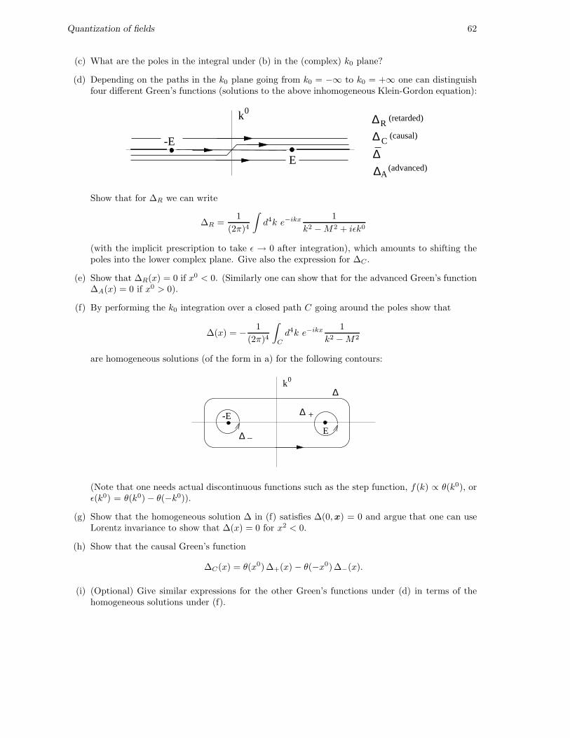
Quantization of fields 62
(c) What are the poles in the integral under (b) in the (complex) k0 plane?
(d) Depending on the paths in the k0 plane going from k0 = −∞ to k0 = +∞ one can distinguishfour different Green’s functions (solutions to the above inhomogeneous Klein-Gordon equation):
k0
-E
E
∆∆∆∆A
C
R(causal)
(advanced)
(retarded)
Show that for ∆R we can write
∆R =1
(2π)4
∫
d4k e−ikx 1
k2 −M2 + iǫk0
(with the implicit prescription to take ǫ → 0 after integration), which amounts to shifting thepoles into the lower complex plane. Give also the expression for ∆C .
(e) Show that ∆R(x) = 0 if x0 < 0. (Similarly one can show that for the advanced Green’s function∆A(x) = 0 if x0 > 0).
(f) By performing the k0 integration over a closed path C going around the poles show that
∆(x) = − 1
(2π)4
∫
C
d4k e−ikx 1
k2 −M2
are homogeneous solutions (of the form in a) for the following contours:
k0
∆ +
∆ _
-E
E
∆
(Note that one needs actual discontinuous functions such as the step function, f(k) ∝ θ(k0), orǫ(k0) = θ(k0) − θ(−k0)).
(g) Show that the homogeneous solution ∆ in (f) satisfies ∆(0,x) = 0 and argue that one can useLorentz invariance to show that ∆(x) = 0 for x2 < 0.
(h) Show that the causal Green’s function
∆C(x) = θ(x0)∆+(x) − θ(−x0)∆−(x).
(i) (Optional) Give similar expressions for the other Green’s functions under (d) in terms of thehomogeneous solutions under (f).
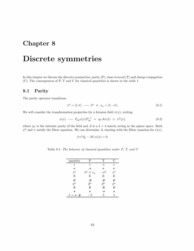
Chapter 8
Discrete symmetries
In this chapter we discuss the discrete symmetries, parity (P), time reversal (T) and charge conjugation(C). The consequences of P, T and C for classical quantities is shown in the table 1.
8.1 Parity
The parity operator transforms
xµ = (t, r) −→ xµ ≡ xµ = (t,−r). (8.1)
We will consider the transformation properties for a fermion field ψ(x), writing
ψ(x) −→ Popψ(x)P−1op = ηPAψ(x) ≡ ψp(x), (8.2)
where ηP is the intrinsic parity of the field and A is a 4 × 4 matrix acting in the spinor space. Bothψp and ψ satisfy the Dirac equation. We can determine A, starting with the Dirac equation for ψ(x),
(iγµ∂µ −M)ψ(x) = 0.
Table 8.1: The behavior of classical quantities under P, T, and C
quantity P T Ct t -t tr -r r r
xµ xµ ≡ xµ −xµ xµ
E E E Ep -p -p p
pµ pµ pµ pµ
L L -L L
s s -s s
λ = s · p −λ λ λ
63
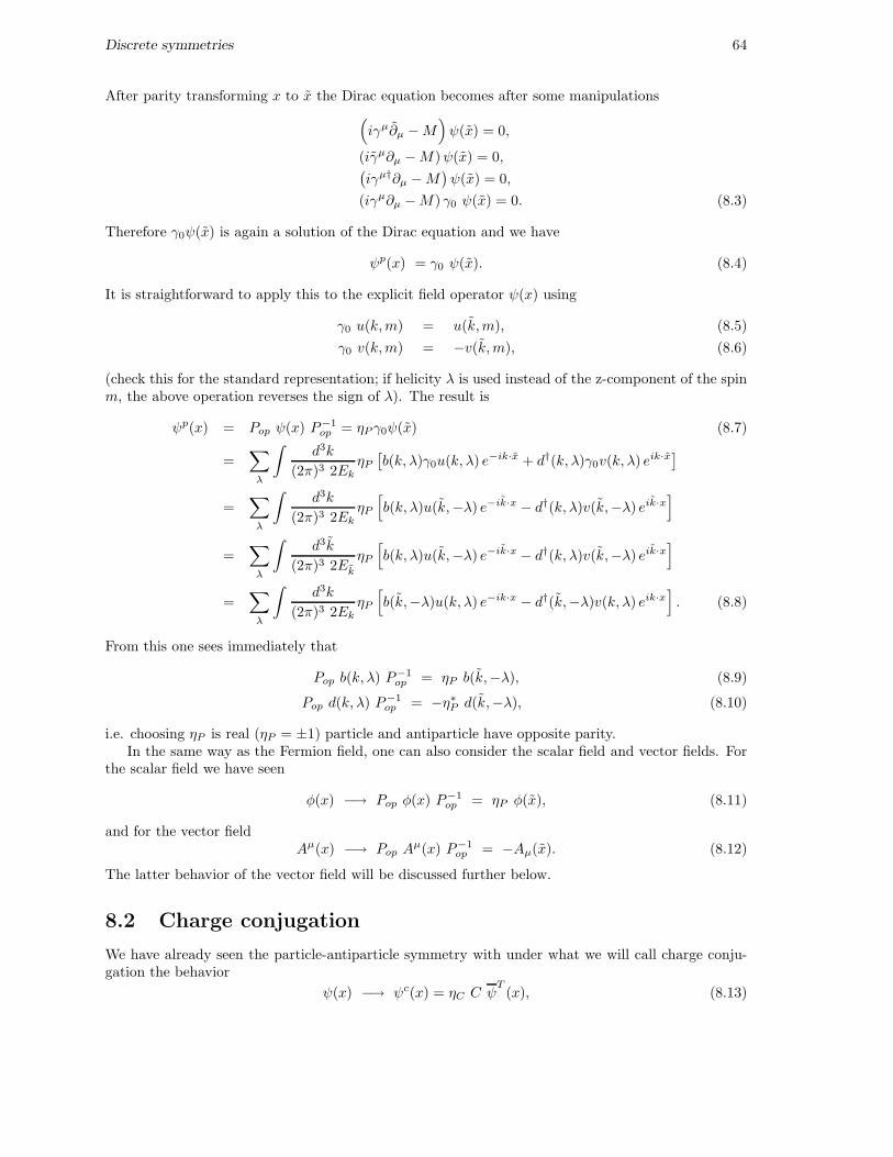
Discrete symmetries 64
After parity transforming x to x the Dirac equation becomes after some manipulations
(
iγµ∂µ −M)
ψ(x) = 0,
(iγµ∂µ −M)ψ(x) = 0,(i㵆∂µ −M
)ψ(x) = 0,
(iγµ∂µ −M) γ0 ψ(x) = 0. (8.3)
Therefore γ0ψ(x) is again a solution of the Dirac equation and we have
ψp(x) = γ0 ψ(x). (8.4)
It is straightforward to apply this to the explicit field operator ψ(x) using
γ0 u(k,m) = u(k,m), (8.5)
γ0 v(k,m) = −v(k,m), (8.6)
(check this for the standard representation; if helicity λ is used instead of the z-component of the spinm, the above operation reverses the sign of λ). The result is
ψp(x) = Pop ψ(x) P−1op = ηPγ0ψ(x) (8.7)
=∑
λ
∫d3k
(2π)3 2EkηP
[b(k, λ)γ0u(k, λ) e
−ik·x + d†(k, λ)γ0v(k, λ) eik·x]
=∑
λ
∫d3k
(2π)3 2EkηP
[
b(k, λ)u(k,−λ) e−ik·x − d†(k, λ)v(k,−λ) eik·x]
=∑
λ
∫d3k
(2π)3 2Ek
ηP
[
b(k, λ)u(k,−λ) e−ik·x − d†(k, λ)v(k,−λ) eik·x]
=∑
λ
∫d3k
(2π)3 2EkηP
[
b(k,−λ)u(k, λ) e−ik·x − d†(k,−λ)v(k, λ) eik·x]
. (8.8)
From this one sees immediately that
Pop b(k, λ) P−1op = ηP b(k,−λ), (8.9)
Pop d(k, λ) P−1op = −η∗P d(k,−λ), (8.10)
i.e. choosing ηP is real (ηP = ±1) particle and antiparticle have opposite parity.In the same way as the Fermion field, one can also consider the scalar field and vector fields. For
the scalar field we have seen
φ(x) −→ Pop φ(x) P−1op = ηP φ(x), (8.11)
and for the vector fieldAµ(x) −→ Pop A
µ(x) P−1op = −Aµ(x). (8.12)
The latter behavior of the vector field will be discussed further below.
8.2 Charge conjugation
We have already seen the particle-antiparticle symmetry with under what we will call charge conju-gation the behavior
ψ(x) −→ ψc(x) = ηC C ψT(x), (8.13)
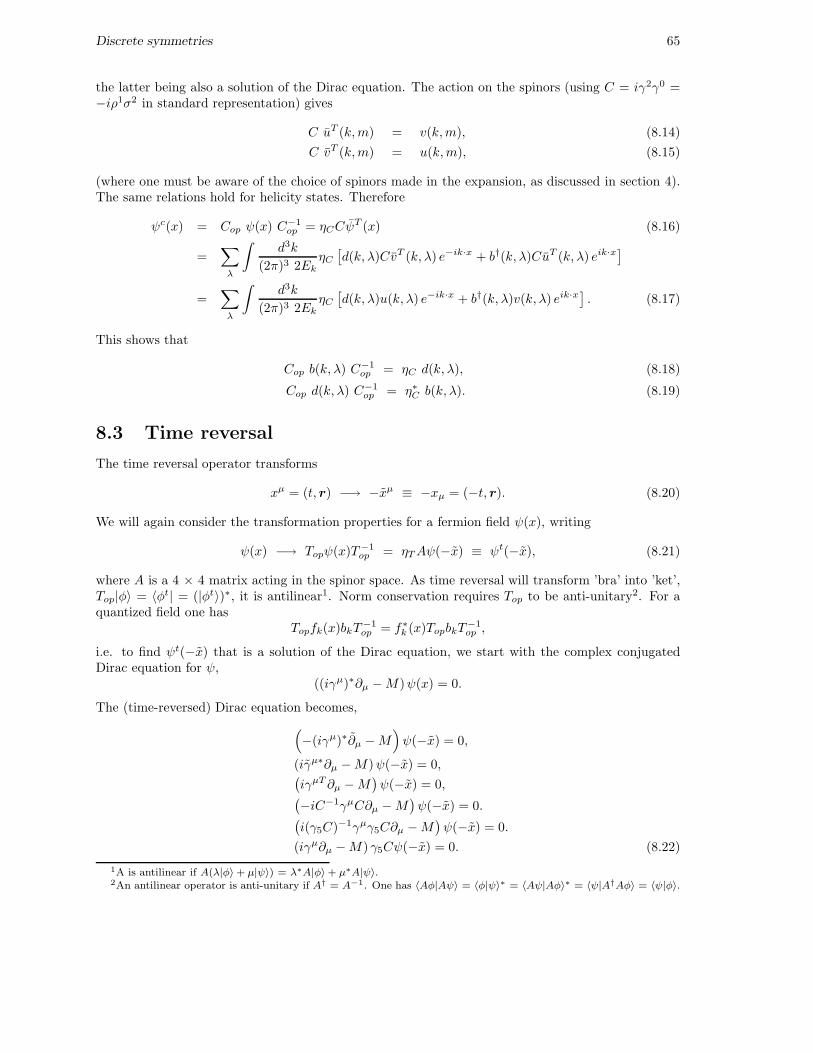
Discrete symmetries 65
the latter being also a solution of the Dirac equation. The action on the spinors (using C = iγ2γ0 =−iρ1σ2 in standard representation) gives
C uT (k,m) = v(k,m), (8.14)
C vT (k,m) = u(k,m), (8.15)
(where one must be aware of the choice of spinors made in the expansion, as discussed in section 4).The same relations hold for helicity states. Therefore
ψc(x) = Cop ψ(x) C−1op = ηCCψ
T (x) (8.16)
=∑
λ
∫d3k
(2π)3 2EkηC
[d(k, λ)CvT (k, λ) e−ik·x + b†(k, λ)CuT (k, λ) eik·x]
=∑
λ
∫d3k
(2π)3 2EkηC
[d(k, λ)u(k, λ) e−ik·x + b†(k, λ)v(k, λ) eik·x] . (8.17)
This shows that
Cop b(k, λ) C−1op = ηC d(k, λ), (8.18)
Cop d(k, λ) C−1op = η∗C b(k, λ). (8.19)
8.3 Time reversal
The time reversal operator transforms
xµ = (t, r) −→ −xµ ≡ −xµ = (−t, r). (8.20)
We will again consider the transformation properties for a fermion field ψ(x), writing
ψ(x) −→ Topψ(x)T−1op = ηTAψ(−x) ≡ ψt(−x), (8.21)
where A is a 4 × 4 matrix acting in the spinor space. As time reversal will transform ’bra’ into ’ket’,Top|φ〉 = 〈φt| = (|φt〉)∗, it is antilinear1. Norm conservation requires Top to be anti-unitary2. For aquantized field one has
Topfk(x)bkT−1op = f∗k (x)TopbkT
−1op ,
i.e. to find ψt(−x) that is a solution of the Dirac equation, we start with the complex conjugatedDirac equation for ψ,
((iγµ)∗∂µ −M)ψ(x) = 0.
The (time-reversed) Dirac equation becomes,
(
−(iγµ)∗∂µ −M)
ψ(−x) = 0,
(iγµ∗∂µ −M)ψ(−x) = 0,(iγµT∂µ −M
)ψ(−x) = 0,
(−iC−1γµC∂µ −M
)ψ(−x) = 0.
(i(γ5C)−1γµγ5C∂µ −M
)ψ(−x) = 0.
(iγµ∂µ −M) γ5Cψ(−x) = 0. (8.22)
1A is antilinear if A(λ|φ〉 + µ|ψ〉) = λ∗A|φ〉 + µ∗A|ψ〉.2An antilinear operator is anti-unitary if A† = A−1. One has 〈Aφ|Aψ〉 = 〈φ|ψ〉∗ = 〈Aψ|Aφ〉∗ = 〈ψ|A†Aφ〉 = 〈ψ|φ〉.
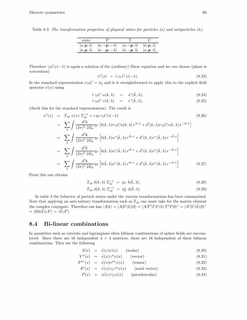
Discrete symmetries 66
Table 8.2: The transformation properties of physical states for particles (a) and antiparticles (a).
state P T C|a; p, λ〉 |a;−p,−λ〉 〈a;−p, λ| |a; p, λ〉|a; p, λ〉 |a;−p,−λ〉 〈a;−p, λ| |a; p, λ〉
Therefore γ5Cψ(−x) is again a solution of the (ordinary) Dirac equation and we can choose (phase isconvention)
ψt(x) = i γ5C ψ(−x). (8.23)
In the standard representation iγ5C = σ2 and it is straightforward to apply this to the explicit fieldoperator ψ(x) using
i γ5C u(k, λ) = u∗(k, λ), (8.24)
i γ5C v(k, λ) = v∗(k, λ), (8.25)
(check this for the standard representation). The result is
ψt(x) = Top ψ(x) T−1op = i ηTγ5Cψ(−x) (8.26)
=∑
λ
∫d3k
(2π)3 2EkηT
[b(k, λ)iγ5Cu(k, λ) e
ik·x + d†(k, λ)iγ5Cv(k, λ) e−ik·x]
=∑
λ
∫d3k
(2π)3 2EkηT
[
b(k, λ)u∗(k, λ) eik·x + d†(k, λ)v∗(k, λ) e−ik·x]
=∑
λ
∫d3k
(2π)3 2EkηT
[
b(k, λ)u∗(k, λ) eik·x + d†(k, λ)v∗(k, λ) e−ik·x]
=∑
λ
∫d3k
(2π)3 2EkηT
[
b(k, λ)u∗(k, λ) eik·x + d†(k, λ)v∗(k, λ) e−ik·x]
(8.27)
From this one obtains
Top b(k, λ) T−1op = ηT b(k, λ), (8.28)
Top d(k, λ) T−1op = η∗T d(k, λ). (8.29)
In table 2 the behavior of particle states under the various transformations has been summarized.Note that applying an anti-unitary transformation such as Top one must take for the matrix element
the complex conjugate. Therefore one has 〈A|k〉 = 〈A|b†(k)|0〉 = 〈A|T †T b†(k)T †T |0〉∗ = 〈At|b†(k)|0〉∗= 〈0|b(k)|At〉 = 〈k|At〉.
8.4 Bi-linear combinations
In quantities such as currents and lagrangians often bilinear combinations of spinor fields are encoun-tered. Since there are 16 independent 4 × 4 matrices, there are 16 independent of these bilinearcombinations. They are the following
S(x) = ψ(x)ψ(x) (scalar) (8.30)
V µ(x) = ψ(x)γµψ(x) (vector) (8.31)
T µν(x) = ψ(x)σµνψ(x) (tensor) (8.32)
Aµ(x) = ψ(x)γ5γµψ(x) (axial vector) (8.33)
P (x) = iψ(x)γ5ψ(x) (pseudoscalar) (8.34)

Discrete symmetries 67
Table 8.3: The behavior of the independent bilinear combinations of fermi fields under P, C, and T
P C T Θ = PCTS(x) S(x) S(x) S(−x) S(−x)V µ(x) Vµ(x) −V µ(x) Vµ(−x) −V µ(−x)T µν(x) Tµν(x) −T µν(x) −Tµν(−x) T µν(−x)Aµ(x) −Aµ(x) Aµ(x) Aµ(−x) −Aµ(−x)P (x) −P (x) P (x) −P (−x) P (−x)
The matrix σµν ≡ (i/2)[γµ, γν ]. The 16 combinations of Dirac matrices appearing above are linearlyindependent. Applying the results from the previous sections it is straightforward to determine thebehavior of the combinations under P, C, and T, as well as under the combined operation Θ = PCT(see Table 3). As the coupling of the photon field to fermions is given by an interaction term in thelagrangian of the form : ψ(x)γµψ(x) : Aµ(x) and behaves as a scalar one sees immediately that thephoton field Aµ(x) behaves in the same way as the vector combination ψ(x)γµψ(x). Note that thelagrangian density L (x) → L (−x) under Θ.
8.5 Form factors
Currents play an important role in field theory. In many applications the expectation values of currentsare needed, e.g. for the vector current V µ(x),
〈p′, s′|V µ(x)|p, s〉. (8.35)
The x-dependence can be accounted for straightforwardly using translation invariance, V µ(x) =ei Pop·xV µ(0)e−i Pop·x. This implies
〈p′|V µ(x)|p〉 = e−i (p−p′)·x〈p′|V µ(0)|p〉. (8.36)
As an example consider the vector current for a point fermion,
V µ(x) =: ψ(x)γµψ(x) :, (8.37)
of which the expectation value between momentum eigenstates can be simply found,
〈p′|V µ(0)|p〉 = u(p′)γµu(p). (8.38)
In general the expectation value between momentum states can be more complicated,
〈p′|V µ(x)|p〉 = u(p′)Γµ(p′, p)u(p) e−i (p−p′)·x, (8.39)
where Γµ(p′, p) can be built from any combination of Dirac matrices (1, γµ, σµν , γ5γµ or γ5), momenta
(pµ or p′µ) or constant tensors (ǫµνρσ or gµν). For instance for nucleons one has
Γµ(p′, p) = γµ F1(q2) +
iσµνqν
2MF2(q
2), (8.40)
where the coefficients are functions of invariants constructed out of the momenta, in this case onlyq2 = (p′ − p)2, called form factors. There are several other terms that also have the correct tensorialbehavior such as
qµ F3(q2),
(pµ + p′µ)
2MF..(q
2),γ5σ
µνqν2M
F..(q2), (8.41)
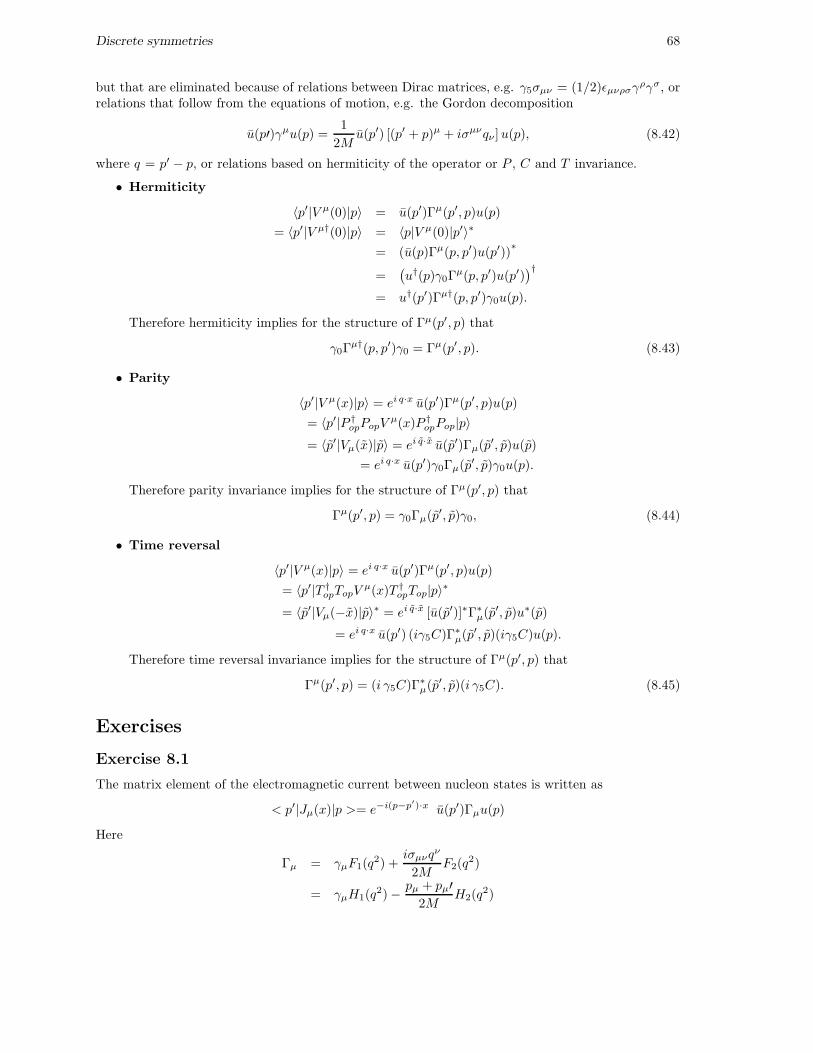
Discrete symmetries 68
but that are eliminated because of relations between Dirac matrices, e.g. γ5σµν = (1/2)ǫµνρσγργσ, or
relations that follow from the equations of motion, e.g. the Gordon decomposition
u(p′)γµu(p) =1
2Mu(p′) [(p′ + p)µ + iσµνqν ]u(p), (8.42)
where q = p′ − p, or relations based on hermiticity of the operator or P , C and T invariance.
• Hermiticity
〈p′|V µ(0)|p〉 = u(p′)Γµ(p′, p)u(p)
= 〈p′|V µ†(0)|p〉 = 〈p|V µ(0)|p′〉∗
= (u(p)Γµ(p, p′)u(p′))∗
=(u†(p)γ0Γ
µ(p, p′)u(p′))†
= u†(p′)Γµ†(p, p′)γ0u(p).
Therefore hermiticity implies for the structure of Γµ(p′, p) that
γ0Γµ†(p, p′)γ0 = Γµ(p′, p). (8.43)
• Parity
〈p′|V µ(x)|p〉 = ei q·x u(p′)Γµ(p′, p)u(p)
= 〈p′|P †opPopVµ(x)P †opPop|p〉
= 〈p′|Vµ(x)|p〉 = ei q·x u(p′)Γµ(p′, p)u(p)
= ei q·x u(p′)γ0Γµ(p′, p)γ0u(p).
Therefore parity invariance implies for the structure of Γµ(p′, p) that
Γµ(p′, p) = γ0Γµ(p′, p)γ0, (8.44)
• Time reversal
〈p′|V µ(x)|p〉 = ei q·x u(p′)Γµ(p′, p)u(p)
= 〈p′|T †opTopVµ(x)T †opTop|p〉∗
= 〈p′|Vµ(−x)|p〉∗ = ei q·x [u(p′)]∗Γ∗µ(p′, p)u∗(p)
= ei q·x u(p′) (iγ5C)Γ∗µ(p′, p)(iγ5C)u(p).
Therefore time reversal invariance implies for the structure of Γµ(p′, p) that
Γµ(p′, p) = (i γ5C)Γ∗µ(p′, p)(i γ5C). (8.45)
Exercises
Exercise 8.1
The matrix element of the electromagnetic current between nucleon states is written as
< p′|Jµ(x)|p >= e−i(p−p′)·x u(p′)Γµu(p)
Here
Γµ = γµF1(q2) +
iσµνqν
2MF2(q
2)
= γµH1(q2) − pµ + pµ′
2MH2(q
2)

Discrete symmetries 69
(a) Use the Dirac equation to prove the Gordon-decomposition
u(p′)γµu(p) =1
2Mu(p′)[(p′ + p)µ + iσµν(p′ − p)ν ]u(p)
(b) Give the relation between Hi en Fi.
(c) Show that hermiticity of the current requires that F1 en F2 are real.
Exercise 8.2
(a) Calculate the current matrix element (using the explicit fermion spinors) in the Breit-frame inwhich q = (0, 0, 0, |q|), p = (E, 0, 0,−|q|/2), p′ = (E, 0, 0, |q|/2) with E2 = M2 + |q|2/4 andexpress them in terms of the Sachs form factors depending on Q2 = −q2,
GE = F1 −Q2
4M2F2,
GM = F1 + F2.
(b) Show that in the interaction with the electromagnetic field,
L int = ejµAµ
the charge is given by eGE(0) and the magnetic moment by eGM (0)/2M .
Exercise 8.3
(a) Show that because of parity conservation no term of the form
γ5σµνqν
2MF3(q
2)
can appear in the current matrix element.
(b) Show that such a term is also not allowed by time-reversal symmetry.
(c) Show that if a term of this form would exist, it would correspond to an electric dipole momentd = −e F3(0)/2M (Interaction term d σ · E).
Chapter 9
Path integrals and quantummechanics
9.1 Time evolution as path integral
The time evolution from t0 → t of a quantum mechanical system is generated by the Hamiltonian,
U(t, t0) = e−i(t−t0)H (9.1)
or
i∂
∂tU(t, t0) = H U(t, t0) (9.2)
Two situations can be distinguished:
(i) Schrodinger picture, in which the operators are time-independent, AS(t) = AS and the statesare time dependent, |ψS(t)〉 = U(t, t0)|ψS(t0)〉,
i∂
∂t|ψS〉 = H |ψS〉, (9.3)
i∂
∂tAS ≡ 0. (9.4)
(ii) Heisenberg picture, in which the states are time-independent, |ψH(t)〉 = |ψH〉, and the operatorsare time-dependent, AH(t) = U−1(t, t0)AH(t0)U(t, t0),
i∂
∂t|ψH〉 ≡ 0, (9.5)
i∂
∂tAH = [AH , H ]. (9.6)
Of these the Heisenberg picture is most appropriate for quantum field theory since the field operatorsdo depend on the position and one would like to have position and time on the same footing.
Consider the two (time-independent) Heisenberg states:
|q, t〉 QH(t)|q, t〉 ≡ q|q, t〉,|q′, t′〉 QH(t′)|q′, t′〉 ≡ q′|q′, t′〉,
(9.7)
70
Path integrals and quantum mechanics 71
and Schrodinger states
|q〉 QS |q〉 ≡ q|q〉,|q′〉 QS |q′〉 ≡ q′|q′〉.
(9.8)
Choose t as the starting point with |q〉 = |q, t〉 and QH(t) = QS and study the evolution of the systemby calculating the quantum mechanical overlap amplitude
〈q′, t′|q, t〉 = 〈q′|e−i H(t′−t)|q〉. (9.9)
Dividing the interval from t ≡ t0 to t′ ≡ tn into n pieces of length ∆τ and using completeness (ateach time ti) one writes
〈q′, t′|q, t〉 = 〈q′|e−i n H∆τ |q〉 = 〈q′|(e−i H∆τ
)n |q〉
=
∫
dq1
∫
. . .
∫
dqn−1 〈q′|e−i H∆τ |qn−1〉 〈qn−1| . . . |q1〉 〈q1|e−i H∆τ |q〉. (9.10)
The purpose of this is to calculate the evolution for an infinitesimal time interval. The hamiltonianis an operator H = H(P,Q) expressed in terms of the operators P and Q. These can be written incoordinate or momentum representation as
Q =
∫
dq |q〉 q 〈q| (9.11)
P =
∫
dq |q〉(
−i ∂∂q
)
〈q| =
∫dp
2π|p〉 p 〈p|, (9.12)
where the transformation between coordinate and momentum space involves
〈q|p〉 = ei p.q. (9.13)
At least for a simple hamiltonian such as consisting of a kinetic energy term and a local potential,H(P,Q) = K(P ) + V (Q) = (P 2/2M) + V (Q) one can split e−i H∆τ ≈ e−i K∆τ e−i V ∆τ , with thecorrection1 being of order (∆τ)2. Then
〈qj+1, tj+1|qj , tj〉 ≈ 〈qj+1|e−i K∆τ e−i V ∆τ |qj〉
=
∫dpj
2π〈qj+1|pj〉 〈pj |e−i K∆τ e−i V ∆τ |qj〉. (9.15)
By letting the kinetic and potential parts act to left and right respectively one can express theexpectation values in terms of integrals containing H(pj , qj), which is a hamiltonian function in whichthe operators are replaced by real-numbered variables. Combining the two terms gives
〈qj+1, tj+1|qj , tj〉 =
∫dpj
2πei pj(qj+1−qj) e−i H(pj ,qj)∆τ
=
∫dpj
2πei pj(qj+1−qj)−i ∆τH(pj ,qj)
=
∫dpj
2πexp (i∆τ [pj qj −H(pj, qj)]) , (9.16)
1For this, use the Campbell-Baker-Hausdorff formula,
eA eB = eC with C = A+B +1
2[A,B] +
1
12[A, [A,B]] +
1
12[[A,B], B] + . . . (9.14)
Path integrals and quantum mechanics 72
or for the full interval
〈q′, t′|q, t〉 =
∫∏
τ
dq(τ) dp(τ)
2πexp
i
t′∑
t
∆τ [pq −H(p, q)]
=
∫
DqDp
2πexp
(
i
∫ t′
t
dτ [pq −H(p, q)]
)
, (9.17)
where Dq and Dp indicate functional integrals. The importance of this expression is that it expressesa quantum mechanical amplitude as a path integral with in the integrand a classical hamiltonianfunction.
Before proceeding we also give the straightforward extension to more than one degree of freedom,
〈q′1, . . . , q′N , t′|q1, . . . , qN , t〉 (9.18)
=
∫(
N∏
n=1
Dqn Dpn
2π
)
exp
(
i
∫ t′
t
dτ
[∑
n
pnqn −H(p1, q1, . . . , pN , qN )
])
.
9.2 Functional integrals
In this section I want to give a fairly heuristic discussion of functional integrals. What one is after isthe meaning of ∫
Dα F [α], (9.19)
where F [α] is a functional that represents a mapping from a function space F of (real) functions α(R → R) into the real numbers R, i.e. F [α] ∈ R. Examples are
F1[α] = α ≡∫
dx α(x),
F2[α] = α2 ≡∫
dx α2(x),
F3[α, β] = αK β ≡∫
dx dy α(x)K(x, y)β(y),
F4[α] = exp
(
−1
2α2
)
≡ exp
(
−1
2
∫
dx α2(x)
)
,
F5[α, α∗] = exp (−α∗K α) ≡ exp
(
−∫
dx dy α∗(x)K(x, y)α(y)
)
.
The kernels K(x, y) in the above examples can be (hermitean) operators acting on the functions,including differential operators, etc.
Two working approaches for functional integration are the following:
(i) the heuristic division of the space on which α acts into cells, i.e. α(x) → αx and F [α] = F (αx)changes into a multivariable function, while
∫
Dα F [α] =
∫(∏
x
dαx
N
)
F (αx) (9.20)
becomes a multidimensional integral.
Path integrals and quantum mechanics 73
(ii) Write α in terms of a sum of orthonormal basis functions, α(x) =∑
n αn fn and K(x, y) =∑
m,n fm(x)Kmn f∗n(y) and consider F [α] = F (αn) as a multivariable function, with
∫
Dα F [α] =
∫(∏
n
dαn
N
)
F (αn) (9.21)
again a multidimensional integral. In both cases N is an appropriately choosen normalizationconstant in such a way that the integral is finite. Note that procedure (i) is an example of themore general procedure under (ii).
Consider the gaussian functional as an example. Using method 1 one writes
∫
Dα exp
(
−1
2α2
)
=
∫(∏
x
dαx
N
)
exp
(
−1
2
∑
x
∆xα2x
)
=∏
x
∫dαx
Nexp
(
−1
2∆xα2
x
)
=∏
x
(
1
N
√
2π
∆x
)
≡ 1. (9.22)
The last equality is obtained by defining the right measure (normalization N) in the integration.Physical answers will usually come out as the ratio of two functional integrals and are thus independentof the chosen measure. Using the second method and expanding in a basis set of functions one obtainsfor the (real) gaussian functional
∫
Dα exp
(
−1
2α2
)
=
∫(∏
n
dαn
N
)
exp
(
−1
2
∑
m,n
αmαn
∫
dx fm(x)fn(x)
)
=∏
n
∫dαn
Nexp
(
−1
2α2
n
)
=∏
n
(√2π
N
)
≡ 1. (9.23)
Having defined the Gaussian integral, the following integrals can be derived for a symmetric or her-mitean kernel K,
∫
Dα exp
(
−1
2αK α
)
=1√
detK(α real-valued) (9.24)
∫
DαDα∗ exp (−α∗K α) =1
detK(α complex-valued) (9.25)
(see Exercises). A useful property of functional integration is the translation invariance,
∫
Dα F [α] =
∫
Dα F [α+ β]. (9.26)
As another important application of translation invariance we mention the identities
∫
Dα exp
(
−1
2α2 − ωα
)
= exp
(1
2ω2
)
, (9.27)
∫
DαDα∗ exp (−α∗α− α∗ω − ω∗α) = exp (ω∗ω) , (9.28)
Path integrals and quantum mechanics 74
Functional differentiation is defined as[
δ
δα(x), α(y)
]
= δ(x− y), (9.29)
or in discretized form
δ
δα(x)−→ 1
∆x
∂
∂αxwith
[∂
∂αx, αy
]
= δxy, (9.30)
δ
δα(x)−→
∑
n
f∗n(x)∂
∂αnwith
[∂
∂αm, αn
]
= δmn. (9.31)
Note that δ(x− y) =∑
n fn(x) f∗n(y). Examples of functional differentiation are
δ
δα(x)α =
δ
δα(x)
∫
dy α(y) =
∫
dy δ(x− y) = 1, (9.32)
δ
δα(x)αKβ =
∫
dy K(x, y)β(y) (9.33)
δ
δα(x)exp
(
−1
2α2
)
= −α(x) exp
(
−1
2α2
)
, (9.34)
δ
δα(x)exp (−αβ) = −β(x) exp (−αβ) . (9.35)
For applications to fermion fields, we need to consider Grassmann-valued functions involving an-ticommuting Grassmann variables, i.e. θη = −ηθ, θ2 = 0. In principle the definitions of functionals isthe same, e.g. the Gaussian-type functionals,
F [θ, θ∗] = exp (−θ∗ θ) ≡ exp
(
−∫
dx θ∗(x) θ(x)
)
,
F [θ, θ∗] = exp (−θ∗K θ) ≡ exp
(
−∫
dx dy θ∗(x)K(x, y) θ(y)
)
.
Integration for Grassmann variables is defined as∫
dθ 1 = 0 and
∫
dθ θ = 1. (9.36)
This gives for the Gaussian functional integral after expanding θ(x) =∑
n θnfn(x) where the coeffi-cients θn are Grassmann variables the result
∫
Dθ∗Dθ exp (−θ∗ θ) =
∫(∏
n
dθ∗n dθn
)
exp
(
−∑
n
θ∗n θn
)
=∏
n
∫
dθ∗n dθn exp (−θ∗n θn)
=∏
n
∫
dθ∗n dθn (1 − θ∗n θn) = 1. (9.37)
We note that from the first to the second line one needs to realize that a pair of different Grassmannvariables behaves as ordinary complex variables. In the expansion of the exponential (from second tothird line), however, products of the same pair appear, which vanish. It is now easy to check that
∫
Dθ∗Dθ exp (−θ∗K θ) = detK. (9.38)
Path integrals and quantum mechanics 75
Functional differentiation of Grassmann-valued functions is given by
δ
δθ(x), θ(y)
= δ(x− y), (9.39)
leading for two Grassmann variables θ and η to e.g.
δ
δη(x)e−θ∗η = θ∗(x) = θ∗(x) e−θ∗η, (9.40)
δ
δη∗(x)e−η∗θ = −θ(x) = −θ(x) e−η∗θ. (9.41)
The translation invariance property and the ’Fourier transform’ identity of Gaussian integrals, remainsin essence the same, e.g.
∫
Dθ∗Dθ exp (−θ∗θ − θ∗η − η∗θ) = exp (η∗η) . (9.42)
9.3 Time ordered products of operators and path integrals
As an example of working with functional integrals consider the expression for K(q′, t′; q, t) for alagrangian L(q, q) = 1
2 q2 − V (q) and the corresponding hamiltonian H(p, q) = 1
2p2 + V (q). The
expression
〈q′, t′|q, t〉 =
∫
DqDp
2πexp
(
i
∫ t′
t
dτ
[
pq − 1
2p2 − V (q)
])
, (9.43)
can be rewritten after rewriting the integrand as − 12 (p − q)2 + 1
2 q2 − V (q) = − 1
2 (p − q)2 + L(q, q).The result is
〈q′, t′|q, t〉 =
∫
Dq exp
(
i
∫ t′
t
dτ L(q, q)
)
, (9.44)
which was considered the starting point for path integral quantization by Feynman.
Note, however, that not always the Dp integration can be removed that easily. A counter exampleis the lagrangian L(q, q) = 1
2q2 f(q) for which H(p, q) = p2/[2f(q)]. As discussed for instance in
Ryder the Dp integration can still be removed but one ends up with an effective lagrangian in thepath integral
〈q′, t′|q, t〉 =
Z
Dq exp
i
Z t′
t
dτ Leff(q, q)
!
, (9.45)
which is of the form Leff (q, q) = L(q, q) − i2δ(0) ln f(q).
Making use of path integrals it is straightforward to calculate the expectation value 〈q′, t′|Q(s)|q, t〉of an operator Q(s) if t ≤ s ≤ t′. By sandwiching the time s in one of the infinitesimal intervals,tj ≤ s ≤ tj+1, we have
〈q′, t′|Q(s)|q, t〉 =
∫∏
i
dqi 〈q′, t′|qn, tn〉 . . .
×〈qj+1, tj+1|Q(s)|qj , tj〉 . . . 〈q1, t1|q, t〉. (9.46)
Using Q(s)|qj , tj〉 = q(s)|qj , tj〉, one gets
〈q′, t′|Q(s)|q, t〉 =
∫
DqDp
2πq(s) exp
(
i
∫ t′
t
dτ [pq −H(p, q)]
)
(9.47)
=
∫
Dq q(s) exp
(
i
∫ t′
t
dτ L(q, q)
)
. (9.48)
Path integrals and quantum mechanics 76
Defining the time ordered product of operators
T Q(t1) . . .Q(tn) ≡ Q(ti1) . . . Q(tin), (9.49)
where ti1 ≥ · · · ≥ tinis a permutation of t1, . . . , tn, one has
〈q′, t′|T Q(t1) . . . Q(tn)|q, t〉
=
∫
Dq q(ti1) . . . q(tin) exp
(
i
∫ t′
t
dτ L(q, q)
)
. (9.50)
Thus not only the quantum mechanical overlap of states can be calculated via a classical path integral,but also expectation of operators, at least if they appear time-ordered.
9.4 An application: time-dependent perturbation theory
From quantum mechanics one should be familiar with the procedure of time-dependent perturbationtheory, the lowest order leading to Fermi’s golden rule. One works in the socalled interaction picture,in which a separation is made of the hamiltonian H = H0 +HI . The fast time evolution is describedin H0 while HI is considered as a perturbation. The interaction picture is defined as
UI(t′, t) ≡ e−i H0(t′−t), (9.51)
ψI(t) ≡ ei H0tψS(t) = ei H0t e−i HtψS(0) = e−iHI tψS(0), (9.52)
AI(t) ≡ ei H0tAS(t)e−i H0t = ei H0tASe−i H0t, (9.53)
i.e. if HI = 0 it is the Heisenberg picture and the evolution 〈q′, t′|q, t〉 is described through theoperators by H0. The evolution of the (interaction) states is described only by HI ,
i∂
∂tψI = HI(t)ψI(t), (9.54)
i∂
∂tAI = [AI , H0], (9.55)
and
ψI(t′) = U(t′, t)ψI(t), (9.56)
i∂
∂tU(t′, t) = HI U(t′, t) (9.57)
with U(t, t) = 1 or
U(t′, t) = 1 − i
∫ t′
t
dτ HI(τ)U(τ, t), (9.58)
which can be solved by iteration, i.e. writing
U(t′, t) =
∞∑
n=0
U (n)(t′, t), (9.59)
one has
U (0)(t′, t) = 1
U (1)(t′, t) = 1 − i
∫ t′
t
dτ HI(τ)U(0)(τ, t) − U (0)(t′, t)
= (−i)∫ t′
t
dτ HI(τ)
Path integrals and quantum mechanics 77
U (2)(t′, t) = 1 − i
∫ t′
t
dτ HI(τ)[
U (0)(τ, t) + U (1)(τ, t)]
−[
U (0)(t′, t) + U (1)(t′, t)]
= (−i)∫ t′
t
dτ HI(τ)U(1)(τ, t)
...
U (n)(t′, t) = (−i)∫ t′
t
dτ HI(τ)U(n−1)(τ, t)
= (−i)n
∫ t′
t
dτ1
∫ τ1
t
dτ2 . . .
∫ τn−1
t
dτn HI(τ1) . . . HI(τn)
=(−i)n
n!
∫ t′
t
dτ1
∫ t′
t
dτ2 . . .
∫ t′
t
dτn T HI(τ1) . . . HI(τn). (9.60)
The last equality is illustrated for the second term U (2) in the following. The integration
Z t′
t
dτ1
Z τ1
t
dτ2 HI(τ1)HI(τ2)
can also be performed by first integrating over τ2 but changing the integration limits (check!).Thus we can write the integration as the sum of the two expressions (multiplying with 1/2),
=1
2
Z t′
t
dτ1
Z τ1
t
dτ2 HI(τ1)HI(τ2)
+1
2
Z t′
t
dτ2
Z t′
τ2
dτ1 HI(τ1)HI(τ2),
Now the integration can be extended by adding theta functions,
=1
2
Z t′
t
dτ1
Z t′
t
dτ2 HI(τ1)HI(τ2)θ(τ1 − τ2)
+1
2
Z t′
t
dτ2
Z t′
t
dτ1 HI(τ1)HI(τ2)θ(τ1 − τ2),
which can be rewritten (by interchanging in the second term the names of the integration variables)
=1
2
Z t′
t
dτ1
Z t′
t
dτ2 [HI(τ1)HI(τ2)θ(τ1 − τ2) +HI(τ2)HI(τ1)θ(τ2 − τ1)] ,
the desired result.
The time evolution operator, therefore, can be written as
U(t′, t) =∞∑
n=0
(−i)n
n!
∫ t′
t
dτ1
∫ t′
t
dτ2 . . .
∫ t′
t
dτn T HI(τ1) . . . HI(τn)
≡ T exp
(
−i∫ t′
t
dτ HI(τ)
)
. (9.61)
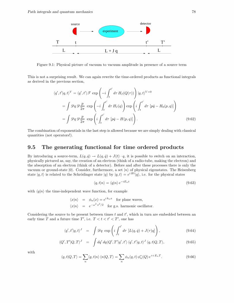
Path integrals and quantum mechanics 78
experiment
L + J q
detectorsource
T t t’ T’
LL
Figure 9.1: Physical picture of vacuum to vacuum amplitude in presence of a source term
This is not a surprising result. We can again rewrite the time-ordered products as functional integralsas derived in the previous section,
〈q′, t′|q, t〉V = 〈q′, t′|T exp
(
−i∫ t′
t
dτ HI(Q(τ))
)
|q, t〉V =0
=
∫
DqDp
2πexp
(
−i∫ t′
t
dτ HI(q)
)
exp
(
i
∫ t′
t
dτ [pq −H0(p, q)]
)
=
∫
DqDp
2πexp
(
i
∫ t′
t
dτ [pq −H(p, q)]
)
. (9.62)
The combination of exponentials in the last step is allowed because we are simply dealing with classicalquantities (not operators!).
9.5 The generating functional for time ordered products
By introducing a source-term, L(q, q) → L(q, q) + J(t) · q, it is possible to switch on an interaction,physically pictured as, say, the creation of an electron (think of a radio-tube, making the electron) andthe absorption of an electron (think of a detector). Before and after these processes there is only thevacuum or ground-state |0〉. Consider, furthermore, a set |n〉 of physical eigenstates. The Heisenbergstate |q, t〉 is related to the Schrodinger state |q〉 by |q, t〉 = ei Ht|q〉, i.e. for the physical states
〈q, t|n〉 = 〈q|n〉 e−iEnt (9.63)
with 〈q|n〉 the time-independent wave function, for example
〈x|n〉 = φn(x) = ei knx for plane waves,
〈x|n〉 = e−ω2 x2/2 for g.s. harmonic oscillator.
Considering the source to be present between times t and t′, which in turn are embedded between anearly time T and a future time T ′, i.e. T < t < t′ < T ′, one has
〈q′, t′|q, t〉J =
∫
Dq exp
(
i
∫ t′
t
dτ [L(q, q) + J(τ)q]
)
, (9.64)
〈Q′, T ′|Q, T 〉J =
∫
dq′ dq〈Q′, T ′|q′, t′〉 〈q′, t′|q, t〉J 〈q, t|Q, T 〉, (9.65)
with〈q, t|Q, T 〉 =
∑
n
〈q, t|n〉 〈n|Q, T 〉 =∑
n
φn(q, t)φ∗n(Q) e+i EnT . (9.66)
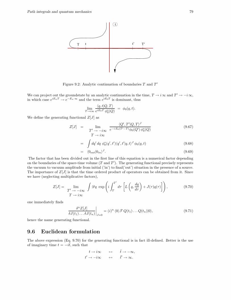
Path integrals and quantum mechanics 79
t
T t t’ T’
Figure 9.2: Analytic continuation of boundaries T and T ′
We can project out the groundstate by an analytic continuation in the time, T → i∞ and T ′ → −i∞,in which case eiEnT → e−En·∞ and the term eiE0T is dominant, thus
limT→i∞
〈q, t|Q, T 〉eiE0T φ∗0(Q)
= φ0(q, t).
We define the generating functional Z[J ] as
Z[J ] = limT ′ → −i∞T → i∞
〈Q′, T ′|Q, T 〉Je−i E0(T ′−T )φ0(Q′)φ∗0(Q)
(9.67)
=
∫
dq′ dq φ∗0(q′, t′)〈q′, t′|q, t〉J φ0(q, t) (9.68)
= 〈0out|0in〉J . (9.69)
The factor that has been divided out in the first line of this equation is a numerical factor dependingon the boundaries of the space-time volume (T and T ′). The generating functional precisely representsthe vacuum to vacuum amplitude from initial (’in’) to final(’out’) situation in the presence of a source.The importance of Z[J ] is that the time ordered product of operators can be obtained from it. Sincewe have (neglecting multiplicative factors),
Z[J ] = limT ′ → −i∞T → i∞
∫
Dq exp
(
i
∫ T ′
T
dτ
[
L
(
q,dq
dτ
)
+ J(τ)q(τ)
])
, (9.70)
one immediately finds
δnZ[J ]
δJ(t1) . . . δJ(tn)
∣∣∣∣J=0
= (i)n 〈0|T Q(t1) . . . Q(tn)|0〉, (9.71)
hence the name generating functional.
9.6 Euclidean formulation
The above expression (Eq. 9.70) for the generating functional is in fact ill-defined. Better is the useof imaginary time t = −it, such that
t→ i∞ ↔ t→ −∞,
t′ → −i∞ ↔ t′ → ∞.
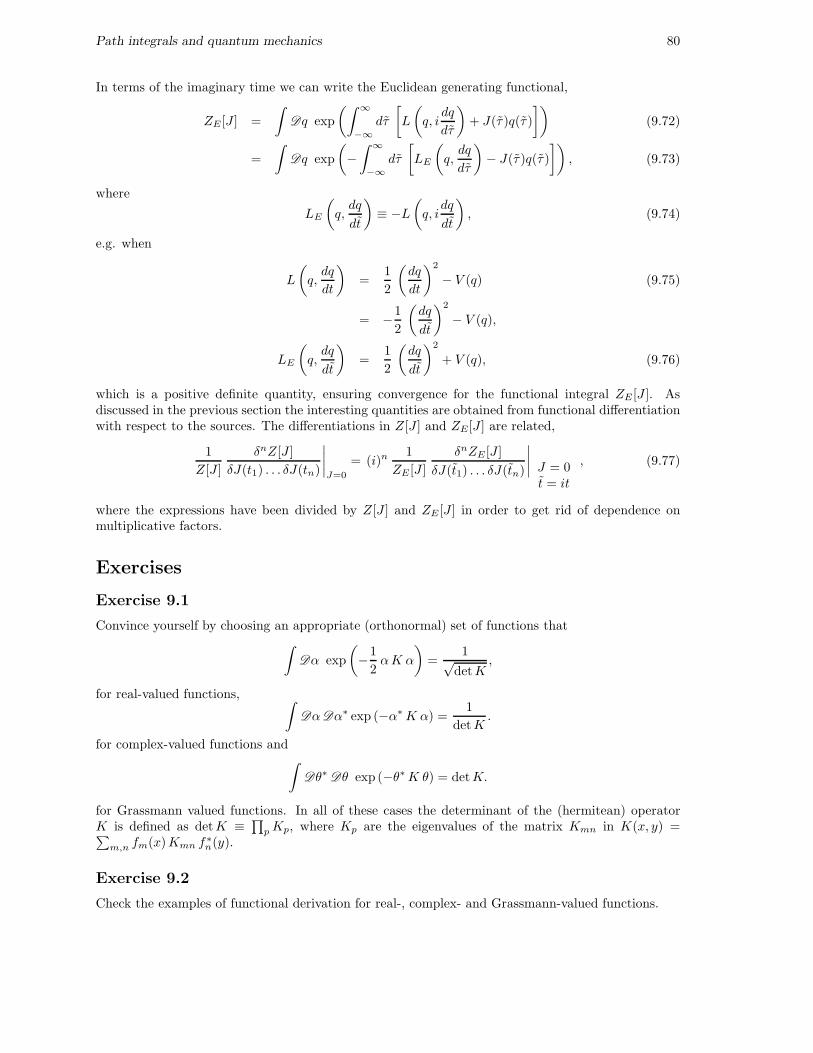
Path integrals and quantum mechanics 80
In terms of the imaginary time we can write the Euclidean generating functional,
ZE [J ] =
∫
Dq exp
(∫ ∞
−∞dτ
[
L
(
q, idq
dτ
)
+ J(τ )q(τ )
])
(9.72)
=
∫
Dq exp
(
−∫ ∞
−∞dτ
[
LE
(
q,dq
dτ
)
− J(τ )q(τ )
])
, (9.73)
where
LE
(
q,dq
dt
)
≡ −L(
q, idq
dt
)
, (9.74)
e.g. when
L
(
q,dq
dt
)
=1
2
(dq
dt
)2
− V (q) (9.75)
= −1
2
(dq
dt
)2
− V (q),
LE
(
q,dq
dt
)
=1
2
(dq
dt
)2
+ V (q), (9.76)
which is a positive definite quantity, ensuring convergence for the functional integral ZE [J ]. Asdiscussed in the previous section the interesting quantities are obtained from functional differentiationwith respect to the sources. The differentiations in Z[J ] and ZE[J ] are related,
1
Z[J ]
δnZ[J ]
δJ(t1) . . . δJ(tn)
∣∣∣∣J=0
= (i)n 1
ZE [J ]
δnZE [J ]
δJ(t1) . . . δJ(tn)
∣∣∣∣ J = 0t = it
, (9.77)
where the expressions have been divided by Z[J ] and ZE [J ] in order to get rid of dependence onmultiplicative factors.
Exercises
Exercise 9.1
Convince yourself by choosing an appropriate (orthonormal) set of functions that
∫
Dα exp
(
−1
2αK α
)
=1√
detK,
for real-valued functions, ∫
DαDα∗ exp (−α∗K α) =1
detK.
for complex-valued functions and∫
Dθ∗Dθ exp (−θ∗K θ) = detK.
for Grassmann valued functions. In all of these cases the determinant of the (hermitean) operatorK is defined as detK ≡ ∏
pKp, where Kp are the eigenvalues of the matrix Kmn in K(x, y) =∑
m,n fm(x)Kmn f∗n(y).
Exercise 9.2
Check the examples of functional derivation for real-, complex- and Grassmann-valued functions.
Path integrals and quantum mechanics 81
Exercise 9.3
Prove the following relations
∫
Dα exp
(
−1
2αK α− αω
)
=1√
detKexp
(1
2ωK−1 ω
)
, (9.78)
∫
Dα∗Dα exp (−α∗K α− α∗ω − ω∗α) =1
detKexp
(ω∗K−1 ω
), (9.79)
∫
Dθ∗Dθ exp (−θ∗K θ − θ∗η − η∗θ) = detK exp(η∗K−1 η
), (9.80)
where∫dy K(x, y)K−1(y, z) = δ(x − z).

Chapter 10
Feynman diagrams for scatteringamplitudes
10.1 Generating functionals for free scalar fields
The generating functional for quantum fields is a generalization of the results in the previous sectorto a system with more degrees of freedom, i.e. φ(x, t) is considered as a set of quantum operatorsφx(t) in the Heisenberg picture and
〈φ′;x′, t′|φ;x, t〉 =
∫
DφDΠ exp
(
i
∫ t′
t
dτ d3x[
Π(x)φ(x) − H (φ,Π)])
=
∫
Dφ exp
(
i
∫ σ′
σ
d4x L (x)
)
(10.1)
and
Z[J ] = limT → i∞T ′ → −i∞
∫
Dφ exp
(
i
∫ T ′
T
d4x [L (φ, ∂µφ) + Jφ]
)
(10.2)
=
∫
Dφ exp
(
−∫ ∞
−∞d4xE [LE(φ, ∂µφ) − Jφ]
)
(10.3)
The Euclidean formulation is as before, implying at the level of four vectors in coordinate and mo-mentum space (when k · x ≡ kE · xE) for instance
x4 = i x0 = i t k4 = −i k0
x · x = (x0)2 −∑3i=1(x
i)2 = −∑4µ=1(x
µ)2 k · k = (k0)2 −∑3i=1(k
i)2 = −∑4µ=1(k
µ)2
d4xE = i d4x d4kE = −i d4k
L = 12 ∂µφ∂
µφ− 12 M
2 φ2 LE = 12 (∂µ
Eφ)2 + 12 M
2 φ2
Furthermore we find the n-point Green functions
〈0|T φ(x1) . . . φ(xn)|0〉 = (−i)n δnZ[J ]
δJ(x1) . . . δJ(xn)
∣∣∣∣J=0
≡ G(n)(x1, . . . , xn), (10.4)
82
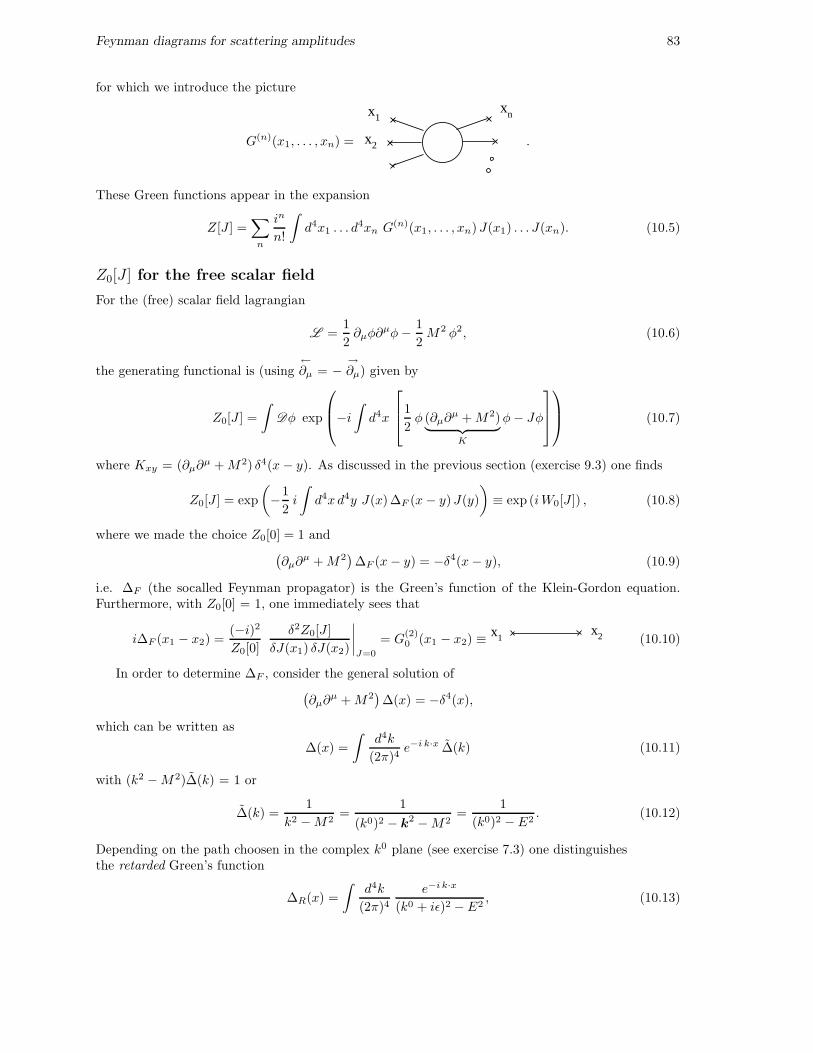
Feynman diagrams for scattering amplitudes 83
for which we introduce the picture
G(n)(x1, . . . , xn) =
x1
x
x
2
n
.
These Green functions appear in the expansion
Z[J ] =∑
n
in
n!
∫
d4x1 . . . d4xn G(n)(x1, . . . , xn)J(x1) . . . J(xn). (10.5)
Z0[J ] for the free scalar field
For the (free) scalar field lagrangian
L =1
2∂µφ∂
µφ− 1
2M2 φ2, (10.6)
the generating functional is (using←∂µ = −
→∂µ) given by
Z0[J ] =
∫
Dφ exp
−i
∫
d4x
1
2φ (∂µ∂
µ +M2)︸ ︷︷ ︸
K
φ− Jφ
(10.7)
where Kxy = (∂µ∂µ +M2) δ4(x− y). As discussed in the previous section (exercise 9.3) one finds
Z0[J ] = exp
(
−1
2i
∫
d4xd4y J(x)∆F (x− y)J(y)
)
≡ exp (iW0[J ]) , (10.8)
where we made the choice Z0[0] = 1 and(∂µ∂
µ +M2)∆F (x− y) = −δ4(x− y), (10.9)
i.e. ∆F (the socalled Feynman propagator) is the Green’s function of the Klein-Gordon equation.Furthermore, with Z0[0] = 1, one immediately sees that
i∆F (x1 − x2) =(−i)2Z0[0]
δ2Z0[J ]
δJ(x1) δJ(x2)
∣∣∣∣J=0
= G(2)0 (x1 − x2) ≡ x1
x2 (10.10)
In order to determine ∆F , consider the general solution of(∂µ∂
µ +M2)∆(x) = −δ4(x),
which can be written as
∆(x) =
∫d4k
(2π)4e−i k·x ∆(k) (10.11)
with (k2 −M2)∆(k) = 1 or
∆(k) =1
k2 −M2=
1
(k0)2 − k2 −M2=
1
(k0)2 − E2. (10.12)
Depending on the path choosen in the complex k0 plane (see exercise 7.3) one distinguishesthe retarded Green’s function
∆R(x) =
∫d4k
(2π)4e−i k·x
(k0 + iǫ)2 − E2, (10.13)
Feynman diagrams for scattering amplitudes 84
satisfying ∆R(x, t) = 0 for t < 0,the advanced Green’s function
∆A(x) =
∫d4k
(2π)4e−i k·x
(k0 − iǫ)2 − E2, (10.14)
satisfying ∆A(x, t) = 0 for t > 0,the causal Green’s function
∆C(x) =
∫d4k
(2π)4e−i k·x
(k0)2 − E2 + iǫ=
∫d4k
(2π)4e−i k·x
k2 −M2 + iǫ, (10.15)
and finally the Green’s function
∆(x) = P
∫d4k
(2π)4e−i k·x
k2 −M2. (10.16)
They are solutions of the inhomogeneous equation. The solution of the homogeneous equation(∂µ∂
µ +M2)∆(x) = 0 can also be written as an integral in k-space,
∆(x) = −∫
C
d4k
(2π)4e−i k·x
k2 −M2, (10.17)
where C is a closed contour in the complex k0-plane. The contours for
i∆(x) = [φ(x), φ(0)] = i∆+(x) + i∆−(x)
i∆+(x) = [φ+(x), φ−(0)] =
∫d3k
(2π)3 2Ee−i k·x
i∆−(x) = [φ−(x), φ+(0)] =
∫d3k
(2π)3 2Ee−i k·x
are also shown in exercise (7.3). It is straightforward (closing contours in the appropriate half of thecomplex plane) to prove for instance that
i∆C(x) = θ(x0) i∆+(x) − θ(−x0) i∆−(x). (10.18)
Thus we see various solutions. In order to see which is the appropriate Green’s function to beused in the generating functional Z0[J ] we will take two routes. The first possibility is to consider thewell-defined Euclidean formulation, the second is to explicitly consider 〈0|T φ(x1)φ(x2)|0〉.
• Firstly, in the (well-defined) Euclidean formulation starting with LE = 12 (∂µ
Eφ)2 + 12 M
2 φ2 -Jφ with the equation of motion
((∂µ
E)2 −M2)φ(x) = −J(x), the generating functional can be
written
Z0[J ] =
∫
Dφ exp
(∫
d4xE
[1
2φ(∂µ
E∂µE −M2
)φ+ Jφ
])
(10.19)
= exp
(
−1
2
∫
d4xE d4yE J(x) (−i∆F (x − y))J(y)
)
, (10.20)
where((∂µ
E)2 −M2)(i∆F (x− y)) = −δ4(x− y) (10.21)
or (see fig. 10.1 for countours)
∆F (x) = −i∫ k0
E=∞
k0E=−∞
d4kE
(2π)4e−i kE ·xE
k2E +M2
(10.22)
=
∫ k0=i∞
k0=−i∞
d4k
(2π)4e−i k·x
k2 −M2, (10.23)
where the latter contour can be deformed to the contour for ∆C , i.e. ∆F = ∆C .
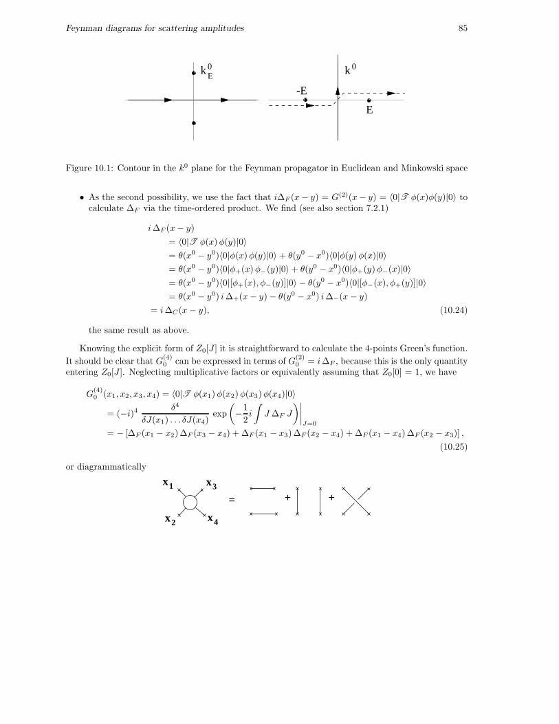
Feynman diagrams for scattering amplitudes 85
k E0
k 0
-E
E
Figure 10.1: Contour in the k0 plane for the Feynman propagator in Euclidean and Minkowski space
• As the second possibility, we use the fact that i∆F (x− y) = G(2)(x− y) = 〈0|T φ(x)φ(y)|0〉 tocalculate ∆F via the time-ordered product. We find (see also section 7.2.1)
i∆F (x− y)
= 〈0|T φ(x)φ(y)|0〉= θ(x0 − y0)〈0|φ(x)φ(y)|0〉 + θ(y0 − x0)〈0|φ(y)φ(x)|0〉= θ(x0 − y0)〈0|φ+(x)φ−(y)|0〉 + θ(y0 − x0)〈0|φ+(y)φ−(x)|0〉= θ(x0 − y0)〈0|[φ+(x), φ−(y)]|0〉 − θ(y0 − x0)〈0|[φ−(x), φ+(y)]|0〉= θ(x0 − y0) i∆+(x− y) − θ(y0 − x0) i∆−(x− y)
= i∆C(x− y), (10.24)
the same result as above.
Knowing the explicit form of Z0[J ] it is straightforward to calculate the 4-points Green’s function.
It should be clear that G(4)0 can be expressed in terms of G
(2)0 = i∆F , because this is the only quantity
entering Z0[J ]. Neglecting multiplicative factors or equivalently assuming that Z0[0] = 1, we have
G(4)0 (x1, x2, x3, x4) = 〈0|T φ(x1)φ(x2)φ(x3)φ(x4)|0〉
= (−i)4 δ4
δJ(x1) . . . δJ(x4)exp
(
−1
2i
∫
J ∆F J
)∣∣∣∣J=0
= − [∆F (x1 − x2)∆F (x3 − x4) + ∆F (x1 − x3)∆F (x2 − x4) + ∆F (x1 − x4)∆F (x2 − x3)] ,
(10.25)
or diagrammatically
x1
x2
x3
x4
= + +
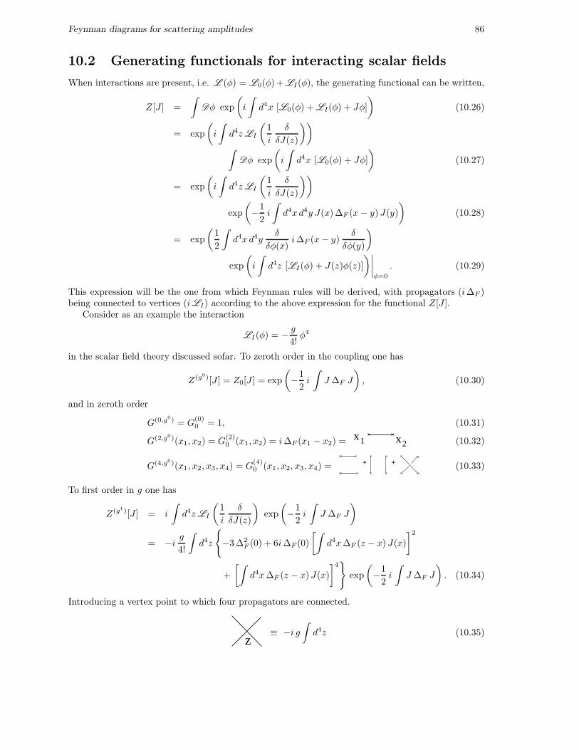
Feynman diagrams for scattering amplitudes 86
10.2 Generating functionals for interacting scalar fields
When interactions are present, i.e. L (φ) = L0(φ)+ LI(φ), the generating functional can be written,
Z[J ] =
∫
Dφ exp
(
i
∫
d4x [L0(φ) + LI(φ) + Jφ]
)
(10.26)
= exp
(
i
∫
d4zLI
(1
i
δ
δJ(z)
))
∫
Dφ exp
(
i
∫
d4x [L0(φ) + Jφ]
)
(10.27)
= exp
(
i
∫
d4zLI
(1
i
δ
δJ(z)
))
exp
(
−1
2i
∫
d4xd4y J(x)∆F (x− y)J(y)
)
(10.28)
= exp
(1
2
∫
d4xd4yδ
δφ(x)i∆F (x− y)
δ
δφ(y)
)
exp
(
i
∫
d4z [LI(φ) + J(z)φ(z)]
)∣∣∣∣φ=0
. (10.29)
This expression will be the one from which Feynman rules will be derived, with propagators (i∆F )being connected to vertices (iLI) according to the above expression for the functional Z[J ].
Consider as an example the interaction
LI(φ) = − g
4!φ4
in the scalar field theory discussed sofar. To zeroth order in the coupling one has
Z(g0)[J ] = Z0[J ] = exp
(
−1
2i
∫
J ∆F J
)
, (10.30)
and in zeroth order
G(0,g0) = G(0)0 = 1, (10.31)
G(2,g0)(x1, x2) = G(2)0 (x1, x2) = i∆F (x1 − x2) = x x21 (10.32)
G(4,g0)(x1, x2, x3, x4) = G(4)0 (x1, x2, x3, x4) = + + (10.33)
To first order in g one has
Z(g1)[J ] = i
∫
d4zLI
(1
i
δ
δJ(z)
)
exp
(
−1
2i
∫
J ∆F J
)
= −i g4!
∫
d4z
−3 ∆2F (0) + 6i∆F (0)
[∫
d4x∆F (z − x)J(x)
]2
+
[∫
d4x∆F (z − x)J(x)
]4
exp
(
−1
2i
∫
J ∆F J
)
. (10.34)
Introducing a vertex point to which four propagators are connected.
z≡ −i g
∫
d4z (10.35)
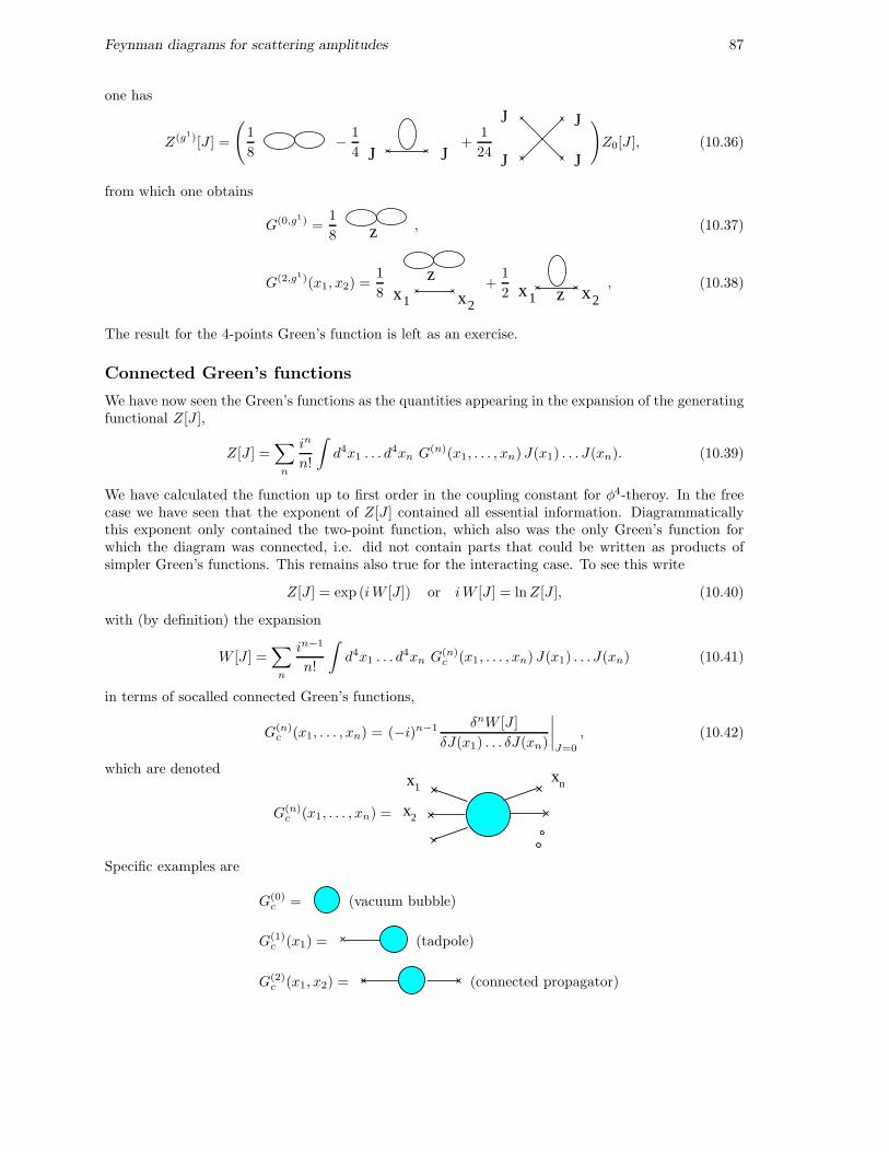
Feynman diagrams for scattering amplitudes 87
one has
Z(g1)[J ] =
(
1
8− 1
4 J J+
1
24
J
J
J
J
)
Z0[J ], (10.36)
from which one obtains
G(0,g1) =1
8 z , (10.37)
G(2,g1)(x1, x2) =1
8z
x x21+
1
2 zx x21, (10.38)
The result for the 4-points Green’s function is left as an exercise.
Connected Green’s functions
We have now seen the Green’s functions as the quantities appearing in the expansion of the generatingfunctional Z[J ],
Z[J ] =∑
n
in
n!
∫
d4x1 . . . d4xn G(n)(x1, . . . , xn)J(x1) . . . J(xn). (10.39)
We have calculated the function up to first order in the coupling constant for φ4-theroy. In the freecase we have seen that the exponent of Z[J ] contained all essential information. Diagrammaticallythis exponent only contained the two-point function, which also was the only Green’s function forwhich the diagram was connected, i.e. did not contain parts that could be written as products ofsimpler Green’s functions. This remains also true for the interacting case. To see this write
Z[J ] = exp (iW [J ]) or iW [J ] = lnZ[J ], (10.40)
with (by definition) the expansion
W [J ] =∑
n
in−1
n!
∫
d4x1 . . . d4xn G(n)
c (x1, . . . , xn)J(x1) . . . J(xn) (10.41)
in terms of socalled connected Green’s functions,
G(n)c (x1, . . . , xn) = (−i)n−1 δnW [J ]
δJ(x1) . . . δJ(xn)
∣∣∣∣J=0
, (10.42)
which are denoted
G(n)c (x1, . . . , xn) =
x1
x
x
2
n
Specific examples are
G(0)c = (vacuum bubble)
G(1)c (x1) = (tadpole)
G(2)c (x1, x2) = (connected propagator)
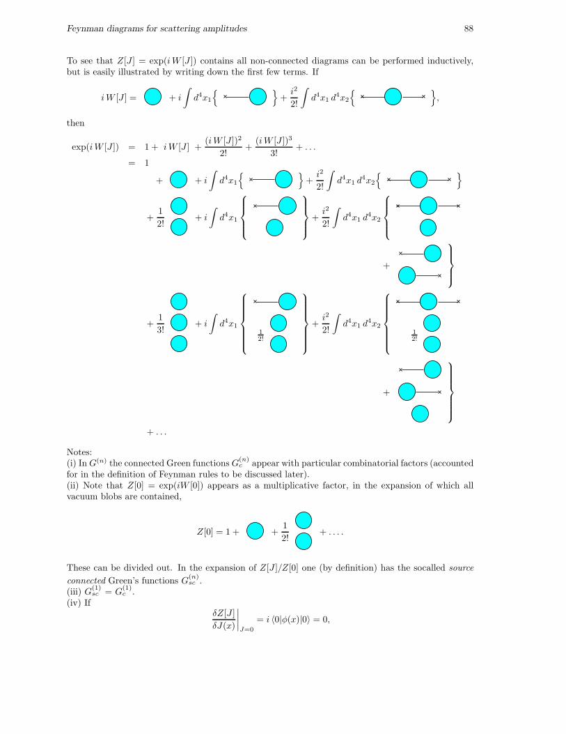
Feynman diagrams for scattering amplitudes 88
To see that Z[J ] = exp(iW [J ]) contains all non-connected diagrams can be performed inductively,but is easily illustrated by writing down the first few terms. If
iW [J ] = + i
∫
d4x1
+i2
2!
∫
d4x1 d4x2
,
then
exp(iW [J ]) = 1 + iW [J ] +(iW [J ])2
2!+
(iW [J ])3
3!+ . . .
= 1
+ + i
∫
d4x1
+i2
2!
∫
d4x1 d4x2
+1
2!+ i
∫
d4x1
+i2
2!
∫
d4x1 d4x2
+
+1
3!+ i
∫
d4x1
12!
+i2
2!
∫
d4x1 d4x2
12!
+
+ . . .
Notes:(i) In G(n) the connected Green functions G
(n)c appear with particular combinatorial factors (accounted
for in the definition of Feynman rules to be discussed later).(ii) Note that Z[0] = exp(iW [0]) appears as a multiplicative factor, in the expansion of which allvacuum blobs are contained,
Z[0] = 1 + +1
2!+ . . . .
These can be divided out. In the expansion of Z[J ]/Z[0] one (by definition) has the socalled source
connected Green’s functions G(n)sc .
(iii) G(1)sc = G
(1)c .
(iv) IfδZ[J ]
δJ(x)
∣∣∣∣J=0
= i 〈0|φ(x)|0〉 = 0,
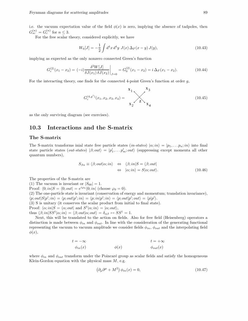
Feynman diagrams for scattering amplitudes 89
i.e. the vacuum expectation value of the field φ(x) is zero, implying the absence of tadpoles, then
G(n)sc = G
(n)c for n ≤ 3.
For the free scalar theory, considered explicitly, we have
W0[J ] = −1
2
∫
d4xd4y J(x)∆F (x− y)J(y), (10.43)
implying as expected as the only nonzero connected Green’s function
G(2)c (x1 − x2) = (−i) δ2W [J ]
δJ(x1) δJ(x2)
∣∣∣∣J=0
= G(2)0 (x1 − x2) = i∆F (x1 − x2). (10.44)
For the interacting theory, one finds for the connected 4-point Green’s function at order g,
G(4,g1)c (x1, x2, x3, x4) =
z
x
x
x
x
3
42
1
(10.45)
as the only surviving diagram (see exercises).
10.3 Interactions and the S-matrix
The S-matrix
The S-matrix transforms inial state free particle states (in-states) |α; in〉 = |p1, . . . pn; in〉 into finalstate particle states (out-states) |β; out〉 = |p′1, . . . p′m; out〉 (suppressing except momenta all otherquantum numbers),
Sβα ≡ 〈β; out|α; in〉 ⇔ 〈β; in|S = 〈β; out|⇔ |α; in〉 = S|α; out〉. (10.46)
The properties of the S-matrix are(1) The vacuum is invariant or |S00| = 1.Proof: 〈0; in|S = 〈0; out| = eiϕ0〈0; in| (choose ϕ0 = 0).(2) The one-particle state is invariant (conservation of energy and momentum; translation invariance),〈p; out|S|p′; in〉 = 〈p; out|p′; in〉 = 〈p; in|p′; in〉 = 〈p; out|p′; out〉 = 〈p|p′〉.(3) S is unitary (it conserves the scalar product from initial to final state).Proof: 〈α; in|S = 〈α; out| and S†|α; in〉 = |α; out〉,thus 〈β; in|SS†|α; in〉 = 〈β; out|α; out〉 = δαβ ↔ SS† = 1.
Next, this will be translated to the action on fields. Also for free field (Heisenberg) operators adistinction is made between φin and φout. In line with the consideration of the generating functionalrepresenting the vacuum to vacuum amplitude we consider fields φin, φout and the interpolating fieldφ(x),
t = −∞ t = +∞φin(x) φ(x) φout(x)
where φin and φout transform under the Poincare group as scalar fields and satisfy the homogeneousKlein-Gordon equation with the physical mass M , e.g.
(∂µ∂
µ +M2)φin(x) = 0, (10.47)
Feynman diagrams for scattering amplitudes 90
while φ satisfies the inhomogeneous Klein-Gordon equation with the bare mass M0 (this is the massappearing in the lagrangian L0),
(∂µ∂
µ +M20
)φ(x) = J(x). (10.48)
The fact that φin and φout satisfy the homogeneous Klein-Gordon equation with the physical massM implies that they create particles and antiparticles as discussed, e.g.
φin(x) =
∫d3k
(2π)3 2E
[a(k) fk(x) + a†(k) f∗k (x)
]. (10.49)
The field φ can be expressed in φin/out using retarded or advanced Green’s functions,
(∂µ∂
µ +M2)φ(x) = J(x) + (M2 −M2
0 )φ(x) = J(x) (10.50)
φ(x) =√Zφin(x) −
∫
d4y∆R(x − y) J(y)
=√Zφin(x) −
∫
d4y d4z∆R(x− y)K(y, z)φ(z) (10.51)
φ(x) =√Zφout(x) −
∫
d4y d4z∆A(x− y)K(y, z)φ(z). (10.52)
Although the above, as it stands, implies the strong (operator) convergence φ(x) →√Zφin(x), this
can actually not be used as it would imply [φ(x), φ(y)] = Z [φin(x), φin(y)] = iZ∆(x− y), a causalitycondition that can be proven to imply the absence of interactions. The convergence therefore mustbe weakened to
〈α|φf (t)β〉 t→−∞−→√Z〈α|φf
in(t)β〉 (10.53)
for normalizable states |α〉 and |β〉 and φf (t) ≡∫d3(x) f∗(x) i
↔∂ 0 φ(x) with f a normalizable solution
of the Klein-Gordon equation (wave packet). Considering plane waves one sees from
〈0|φ(x)|p〉 = limt→∞
√Z 〈0|φout(x)|p〉 =
√Z e−i p·x
= limt→−∞
√Z 〈0|φin(x)|p〉 =
√Z e−i p·x
that identical normalization of (single-particle) plane waves in initial and final state implies the samewave function normalization Z for in and out fields.
The relation between S-matrix and in- and out-fields is: φin(x) = S φout(x)S−1.
Proof:
〈β; out|φout =
〈β; in|φinS〈β; in|Sφout
→ φin S = S φout(x).
Finally we check that as expected S does not spoil Poincare invariance, i.e. S is invariant underPoincare transformations: U(Λ, a)SU−1(Λ, a) = S.Proof: φin(Λx+ a) = Uφin(x)U−1 = USφout(x)S
−1U−1 = US U−1U φout(x)U−1U S−1U−1
= USU−1 φout(Λx+ a)US−1U−1 ⇔ USU−1 = S.
The relation between S and Z[J ]
To establish this relation, the source term Jφ in the lagrangian density is treated in the interactionpicture. The time evolution operator (see Eq. 9.62) is then
UT ′
T [J ] = T exp
(
i
∫ T ′
T
d4xJ(x)φ(x)
)
, (10.54)
Feynman diagrams for scattering amplitudes 91
and satisfies the propertyδUT ′
T [J ]
δJ(x)= i UT ′
t [J ]φ(x)U tT [J ], (10.55)
or for U [J ] ≡ U∞−∞[J ]
δU [J ]
δJ(x)= i U∞t [J ]φ(x)U t
−∞[J ] (10.56)
t→∞−→ i φ(x)U [J ] → i√Z φout(x)U [J ]
t→−∞−→ i U [J ]φ(x) → i√Z U [J ]φin(x).
Since δU [J ]/δJ(x) satisfies the same equations as φ(x) and we know the limits, we can, just as we didfor φ(x), express it in terms of advanced and retarded Green’s functions,
δU [J ]
δJ(x)= i
√Z U [J ]φin(x) −
∫
d4y d4z∆R(x − y)K(y, z)δU [J ]
δJ(z)
= i√Z φout(x)U [J ] −
∫
d4y d4z∆A(x− y)K(y, z)δU [J ]
δJ(z).
Taking the difference between the two expressions
√Z (φout(x)U [J ] − U [J ]φin(x))
= i
∫
d4y d4z (∆R(x− y) − ∆A(x− y))K(y, z)δU [J ]
δJ(z), (10.57)
or
[φin(x), S U [J ]] =i√Z
∫
d4y d4z∆(x − y)K(y, z)δ
δJ(z)S U [J ]. (10.58)
In order to find a solution to this equation note that, with the use of the Baker-Campbell-Hausdorffformula e−B Ae+B = A+ [A,B] (for the case that [A,B] is a c-number), one has
[A, eB ] = [A,B]eB, (10.59)
[A, eB eC ] = [A,B + C]eB eC , (10.60)
provided [A,B] and [A,C] are c-numbers. Thus applied to the field φ(x) = φ+(x) + φ−(x),
[
φ(x), eR
d4x φ−(x) f(x) eR
d4y φ+(y) f(y)]
=
∫
d4y [φ(x), φ(y)] f(y) eR
d4z φ−(z) f(z) eR
d4z φ+(z) f(z),
i.e.[
φ(x), : eR
d4z φ(z) f(z) :]
= i
∫
d4y∆(x − y) f(y) : eR
d4z φ(z) f(z) :, (10.61)
where the normal ordered expression : eR
φ f : is used, which is equal to the expression eR
φ−f eR
φ+f
in which the creation operators are placed left of annihilation operators. Thus
S U [J ] =: exp
(1√Z
∫
d4xd4y φin(x)K(x, y)δ
δJ(y)
)
: F [J ], (10.62)
where F [J ] is some (arbitrary) functional. Noting that 〈0| : eA : |0〉 = 1 it follows that
F [J ] = 〈0|S U [J ]|0〉 = 〈0|U [J ]|0〉 = 〈0out|0in〉 ∝ Z[J ], (10.63)
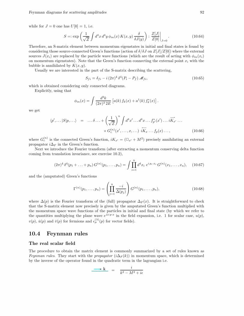
Feynman diagrams for scattering amplitudes 92
while for J = 0 one has U [0] = 1, i.e.
S =: exp
(1√Z
∫
d4xd4y φin(x)K(x, y)δ
δJ(y)
)
:Z[J ]
Z[0]
∣∣∣∣J=0
. (10.64)
Therefore, an S-matrix element between momentum eigenstates in initial and final states is found byconsidering those source-connected Green’s functions (action of δ/δJ on Z[J ]/Z[0]) where the externalsources J(xi) are replaced by the particle wave functions (which are the result of acting with φin(xi)on momentum eigenstates). Note that the Green’s function connecting the external point xi with thebubble is annihilated by K(x, y).
Usually we are interested in the part of the S-matrix describing the scattering,
Sfi = δfi − i (2π)4 δ4(Pi − Pf )Mfi, (10.65)
which is obtained considering only connected diagrams.Explicitly, using that
φin(x) =
∫d3k
(2π)3 2E
[a(k) fk(x) + a†(k) f∗k (x)
].
we get
〈p′, . . . |S|p, . . .〉 = . . . δ . . .+
(1√Z
)n ∫
d4x′ . . . d4x . . . f∗p′(x′) . . .−→iKx′ . . .
×G(n)c (x′, . . . , x, . . .)
←−iKx . . . fp(x) . . . , (10.66)
where G(n)c is the connected Green’s function, iKx′ = (2x′ +M2) precisely annihilating an external
propagator i∆F in the Green’s function.Next we introduce the Fourier transform (after extracting a momentum conserving delta function
coming from translation invariance, see exercise 10.2),
(2π)4 δ4(p1 + . . .+ pn)G(n)(p1, . . . , pn) =
∫ n∏
i=1
d4xi ei pi·xi G(n)(x1, . . . , xn), (10.67)
and the (amputated) Green’s functions
Γ(n)(p1, . . . , pn) =
n∏
j=1
−i∆(pj)
G(n)(p1, . . . , pn), (10.68)
where ∆(p) is the Fourier transform of the (full) propagator ∆F (x). It is straightforward to checkthat the S-matrix element now precisely is given by the amputated Green’s function multiplied withthe momentum space wave functions of the particles in initial and final state (by which we refer tothe quantities multiplying the plane wave e±i p·x in the field expansion, i.e. 1 for scalar case, u(p),
v(p), u(p) and v(p) for fermions and ǫ(λ)µ (p) for vector fields).
10.4 Feynman rules
The real scalar field
The procedure to obtain the matrix element is commonly summarized by a set of rules known asFeynman rules. They start with the propagator (i∆F (k)) in momentum space, which is determinedby the inverse of the operator found in the quadratic term in the lagrangian i.e.
k =i
k2 −M2 + iǫ
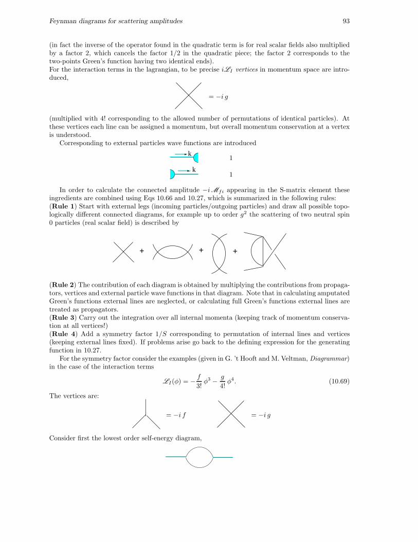
Feynman diagrams for scattering amplitudes 93
(in fact the inverse of the operator found in the quadratic term is for real scalar fields also multipliedby a factor 2, which cancels the factor 1/2 in the quadratic piece; the factor 2 corresponds to thetwo-points Green’s function having two identical ends).For the interaction terms in the lagrangian, to be precise iLI vertices in momentum space are intro-duced,
= −i g
(multiplied with 4! corresponding to the allowed number of permutations of identical particles). Atthese vertices each line can be assigned a momentum, but overall momentum conservation at a vertexis understood.
Corresponding to external particles wave functions are introduced
k1
k1
In order to calculate the connected amplitude −iMfi appearing in the S-matrix element theseingredients are combined using Eqs 10.66 and 10.27, which is summarized in the following rules:(Rule 1) Start with external legs (incoming particles/outgoing particles) and draw all possible topo-logically different connected diagrams, for example up to order g2 the scattering of two neutral spin0 particles (real scalar field) is described by
+ + +
(Rule 2) The contribution of each diagram is obtained by multiplying the contributions from propaga-tors, vertices and external particle wave functions in that diagram. Note that in calculating amputatedGreen’s functions external lines are neglected, or calculating full Green’s functions external lines aretreated as propagators.(Rule 3) Carry out the integration over all internal momenta (keeping track of momentum conserva-tion at all vertices!)(Rule 4) Add a symmetry factor 1/S corresponding to permutation of internal lines and vertices(keeping external lines fixed). If problems arise go back to the defining expression for the generatingfunction in 10.27.
For the symmetry factor consider the examples (given in G. ’t Hooft and M. Veltman, Diagrammar)in the case of the interaction terms
LI(φ) = − f
3!φ3 − g
4!φ4. (10.69)
The vertices are:
= −i f = −i g
Consider first the lowest order self-energy diagram,
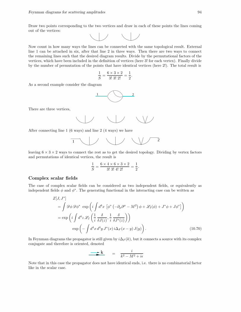
Feynman diagrams for scattering amplitudes 94
Draw two points corresponding to the two vertices and draw in each of these points the lines comingout of the vertices:
Now count in how many ways the lines can be connected with the same topological result. Externalline 1 can be attached in six, after that line 2 in three ways. Then there are two ways to connectthe remaining lines such that the desired diagram results. Divide by the permutational factors of thevertices, which have been included in the definition of vertices (here 3! for each vertex). Finally divideby the number of permutation of the points that have identical vertices (here 2!). The total result is
1
S=
6 × 3 × 2
3! 3! 2!=
1
2.
As a second example consider the diagram
21
There are three vertices,
After connecting line 1 (6 ways) and line 2 (4 ways) we have
1 2
leaving 6 × 3 × 2 ways to connect the rest as to get the desired topology. Dividing by vertex factorsand permutations of identical vertices, the result is
1
S=
6 × 4 × 6 × 3 × 2
3! 3! 4! 2!=
1
2.
Complex scalar fields
The case of complex scalar fields can be considered as two independent fields, or equivalently asindependent fields φ and φ∗. The generating functional in the interacting case can be written as
Z[J, J∗]
=
∫
DφDφ∗ exp
(
i
∫
d4x[φ∗(−∂µ∂
µ −M2)φ+ LI(φ) + J∗φ+ Jφ∗
])
= exp
(
i
∫
d4zLI
(1
i
δ
δJ(z),1
i
δ
δJ∗(z)
))
exp
(
−∫
d4xd4y J∗(x) i∆F (x− y)J(y)
)
. (10.70)
In Feynman diagrams the propagator is still given by i∆F (k), but it connects a source with its complexconjugate and therefore is oriented, denoted
k =i
k2 −M2 + iǫ
Note that in this case the propagator does not have identical ends, i.e. there is no combinatorial factorlike in the scalar case.
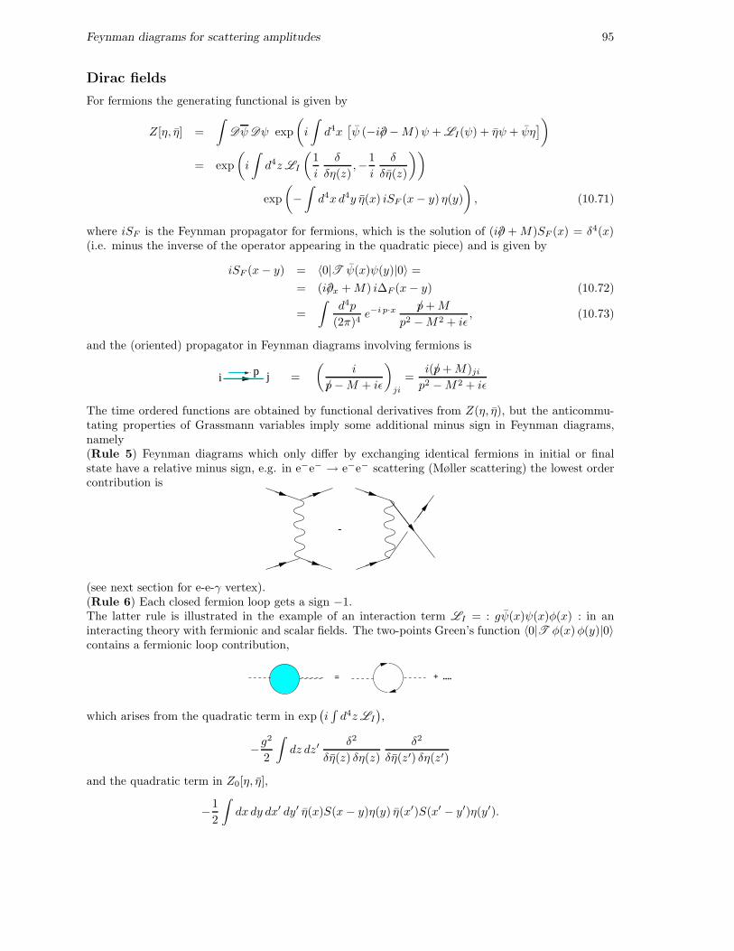
Feynman diagrams for scattering amplitudes 95
Dirac fields
For fermions the generating functional is given by
Z[η, η] =
∫
DψDψ exp
(
i
∫
d4x[ψ (−i/∂ −M)ψ + LI(ψ) + ηψ + ψη
])
= exp
(
i
∫
d4zLI
(1
i
δ
δη(z),−1
i
δ
δη(z)
))
exp
(
−∫
d4xd4y η(x) iSF (x− y) η(y)
)
, (10.71)
where iSF is the Feynman propagator for fermions, which is the solution of (i/∂ +M)SF (x) = δ4(x)(i.e. minus the inverse of the operator appearing in the quadratic piece) and is given by
iSF (x− y) = 〈0|T ψ(x)ψ(y)|0〉 =
= (i/∂x +M) i∆F (x− y) (10.72)
=
∫d4p
(2π)4e−i p·x /p+M
p2 −M2 + iǫ, (10.73)
and the (oriented) propagator in Feynman diagrams involving fermions is
pi j =
(i
/p−M + iǫ
)
ji
=i(/p+M)ji
p2 −M2 + iǫ
The time ordered functions are obtained by functional derivatives from Z(η, η), but the anticommu-tating properties of Grassmann variables imply some additional minus sign in Feynman diagrams,namely(Rule 5) Feynman diagrams which only differ by exchanging identical fermions in initial or finalstate have a relative minus sign, e.g. in e−e− → e−e− scattering (Møller scattering) the lowest ordercontribution is
-
(see next section for e-e-γ vertex).(Rule 6) Each closed fermion loop gets a sign −1.The latter rule is illustrated in the example of an interaction term LI = : gψ(x)ψ(x)φ(x) : in aninteracting theory with fermionic and scalar fields. The two-points Green’s function 〈0|T φ(x)φ(y)|0〉contains a fermionic loop contribution,
= + ....
which arises from the quadratic term in exp(i∫d4zLI
),
−g2
2
∫
dz dz′δ2
δη(z) δη(z)
δ2
δη(z′) δη(z′)
and the quadratic term in Z0[η, η],
−1
2
∫
dx dy dx′ dy′ η(x)S(x − y)η(y) η(x′)S(x′ − y′)η(y′).
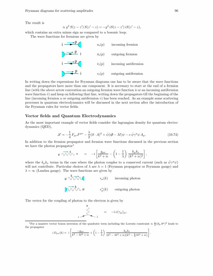
Feynman diagrams for scattering amplitudes 96
The result is∝ g2 S(z − z′)S(z′ − z) = −g2 iS(z − z′) iS(z′ − z),
which contains an extra minus sign as compared to a bosonic loop.The wave functions for fermions are given by
pi ui(p) incoming fermion
pi ui(p) outgoing fermion
pi vi(p) incoming antifermion
pi vi(p) outgoing antifermion
In writing down the expressions for Feynman diagrams one has to be aware that the wave functionsand the propagators have more than one component. It is necessary to start at the end of a fermionline (with the above arrow convention an outgoing fermion wave function u or an incoming antifermionwave function v) and keep on following that line, writing down the propagators till the beginning of theline (incoming fermion u or outgoing antifermion v) has been reached. As an example some scatteringprocesses in quantum electrodynamics will be discussed in the next section after the introduction ofthe Feynman rules for vector fields.
Vector fields and Quantum Electrodynamics
As the most important example of vector fields consider the lagrangian density for quantum electro-dynamics (QED),
L = −1
4FµνF
µν − λ
2(∂ ·A)2 + ψ(i/∂ −M)ψ − e ψγµψAµ. (10.74)
In addition to the fermion propagator and fermion wave functions discussed in the previous sectionwe have the photon propagator1
µ νk
= −i[
gµν
k2 + iǫ−(
1 − 1
λ
)kµkν
(k2 + iǫ)2
]
,
where the kµkν terms in the case where the photon couples to a conserved current (such as ψγµψ)will not contribute. Particular choices of λ are λ = 1 (Feynman propagator or Feynman gauge) andλ = ∞ (Landau gauge). The wave functions are given by
kµ ǫµ(k) incoming photon
kµ ǫ∗µ(k) outgoing photon
The vertex for the coupling of photon to the electron is given by
µ
i j
= −i e(γµ)ji.
1For a massive vector boson inversion of the quadratic term including the Lorentz constraint ∝ λ2(∂µAµ)2 leads to
the propagator
iDµν(k) = i
"
−gµν
k2 −M2 + iǫ+
„
1 − 1
λ
«
kµkν
(k2 −M2 + iǫ)(k2 − 1λM2 + iǫ)
#
.
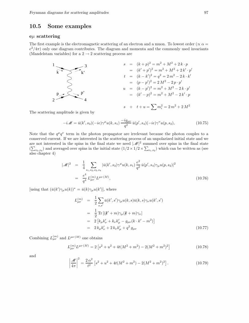
Feynman diagrams for scattering amplitudes 97
10.5 Some examples
eµ scattering
The first example is the electromagnetic scattering of an electron and a muon. To lowest order (∝ α =e2/4π) only one diagram contributes. The diagram and momenta and the commonly used invariants(Mandelstam variables) for a 2 → 2 scattering process are
k k’
p’p
1 3
2 4
s = (k + p)2 = m2 +M2 + 2 k · p= (k′ + p′)2 = m2 +M2 + 2 k′ · p′
t = (k − k′)2 = q2 = 2m2 − 2 k · k′
= (p− p′)2 = 2M2 − 2 p · p′
u = (k − p′)2 = m2 +M2 − 2 k · p′
= (k′ − p)2 = m2 +M2 − 2 k′ · p
s + t+ u =∑
m2i = 2m2 + 2M2
The scattering amplitude is given by
−iM = u(k′, s3)(−ie)γµu(k, s1)−igµν
q2u(p′, s4)(−ie)γνu(p, s2), (10.75)
Note that the qµqν term in the photon propagator are irrelevant because the photon couples to aconserved current. If we are interested in the scattering process of an unpolarized initial state and weare not interested in the spins in the final state we need |M |2 summed over spins in the final state(∑
s3,s4) and averaged over spins in the initial state (1/2× 1/2×
∑
s1,s2) which can be written as (see
also chapter 4)
|M |2 =1
4
∑
s1,s2,s3,s4
|u(k′, s3)γµu(k, s1)e2
q2u(p′, s4)γµu(p, s2)|2
=e4
q4L(m)
µν Lµν (M), (10.76)
[using that (u(k′)γµu(k))∗ = u(k)γµu(k
′)], where
L(m)µν =
1
2
∑
s,s′
u(k′, s′)γµu(k, s)u(k, s)γνu(k′, s′)
=1
2Tr [(/k′ +m)γµ(/k +m)γν ]
= 2[kµk
′ν + kνk
′µ − gµν(k · k′ −m2)
]
= 2 kµk′ν + 2 kνk
′µ + q2 gµν (10.77)
Combining L(m)µν and Lµν (M) one obtains
L(m)µν Lµν (M) = 2
[s2 + u2 + 4t(M2 +m2) − 2(M2 +m2)2
](10.78)
and ∣∣∣∣
M
4π
∣∣∣∣
2
=2α2
t2[s2 + u2 + 4t(M2 +m2) − 2(M2 +m2)2
]. (10.79)
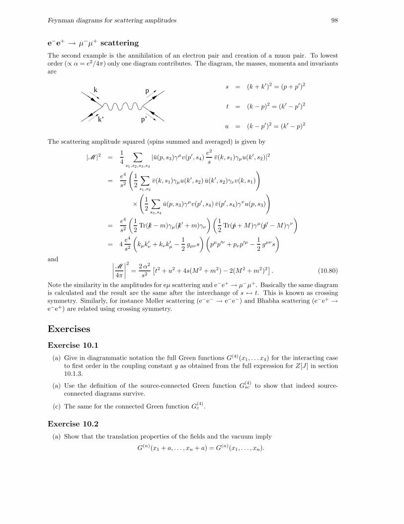
Feynman diagrams for scattering amplitudes 98
e−e+ → µ−µ+ scattering
The second example is the annihilation of an electron pair and creation of a muon pair. To lowestorder (∝ α = e2/4π) only one diagram contributes. The diagram, the masses, momenta and invariantsare
k
k’
p
p’
s = (k + k′)2 = (p+ p′)2
t = (k − p)2 = (k′ − p′)2
u = (k − p′)2 = (k′ − p)2
The scattering amplitude squared (spins summed and averaged) is given by
|M |2 =1
4
∑
s1,s2,s3,s4
|u(p, s3)γµv(p′, s4)e2
sv(k, s1)γµu(k
′, s2)|2
=e4
s2
(
1
2
∑
s1,s2
v(k, s1)γµu(k′, s2) u(k
′, s2)γνv(k, s1)
)
×(
1
2
∑
s3,s4
u(p, s3)γµv(p′, s4) v(p
′, s4)γνu(p, s3)
)
=e4
s2
(1
2Tr(/k −m)γµ(/k′ +m)γν
)(1
2Tr(/p+M)γµ(/p′ −M)γν
)
= 4e4
s2
(
kµk′ν + kνk
′µ − 1
2gµνs
)(
pµp′ν + pνp′µ − 1
2gµνs
)
and ∣∣∣∣
M
4π
∣∣∣∣
2
=2α2
s2[t2 + u2 + 4s(M2 +m2) − 2(M2 +m2)2
]. (10.80)
Note the similarity in the amplitudes for eµ scattering and e−e+ → µ−µ+. Basically the same diagramis calculated and the result are the same after the interchange of s ↔ t. This is known as crossingsymmetry. Similarly, for instance Møller scattering (e−e− → e−e−) and Bhabha scattering (e−e+ →e−e+) are related using crossing symmetry.
Exercises
Exercise 10.1
(a) Give in diagrammatic notation the full Green functions G(4)(x1, . . . x4) for the interacting caseto first order in the coupling constant g as obtained from the full expression for Z[J ] in section10.1.3.
(a) Use the definition of the source-connected Green function G(4)sc to show that indeed source-
connected diagrams survive.
(c) The same for the connected Green function G(4)c .
Exercise 10.2
(a) Show that the translation properties of the fields and the vacuum imply
G(n)(x1 + a, . . . , xn + a) = G(n)(x1, . . . , xn).
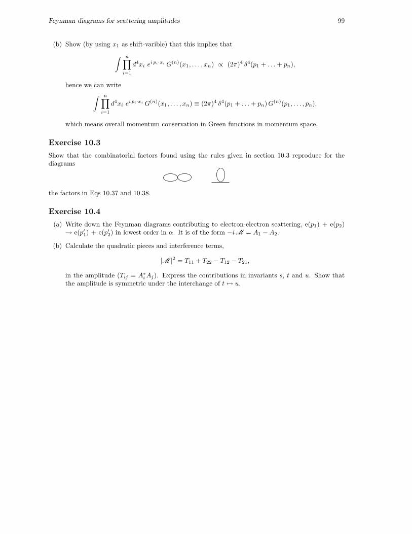
Feynman diagrams for scattering amplitudes 99
(b) Show (by using x1 as shift-varible) that this implies that
∫ n∏
i=1
d4xi ei pi·xi G(n)(x1, . . . , xn) ∝ (2π)4 δ4(p1 + . . .+ pn),
hence we can write
∫ n∏
i=1
d4xi ei pi·xi G(n)(x1, . . . , xn) ≡ (2π)4 δ4(p1 + . . .+ pn)G(n)(p1, . . . , pn),
which means overall momentum conservation in Green functions in momentum space.
Exercise 10.3
Show that the combinatorial factors found using the rules given in section 10.3 reproduce for thediagrams
the factors in Eqs 10.37 and 10.38.
Exercise 10.4
(a) Write down the Feynman diagrams contributing to electron-electron scattering, e(p1) + e(p2)→ e(p′1) + e(p′2) in lowest order in α. It is of the form −iM = A1 −A2.
(b) Calculate the quadratic pieces and interference terms,
|M |2 = T11 + T22 − T12 − T21,
in the amplitude (Tij = A∗iAj). Express the contributions in invariants s, t and u. Show thatthe amplitude is symmetric under the interchange of t↔ u.
Chapter 11
Scattering theory
11.1 kinematics in scattering processes
Phase space
The 1-particle state is denoted |p〉. It is determined by the energy-momentum four vector p = (E,p)which satisfies p2 = E2−p2 =m2. A physical state has positive energy. The phase space is determinedby the weight factors assigned to each state in the summation or integration over states, i.e. the 1-particle phase space is
∫d3p
(2π)3 2E=
∫d4p
(2π)4θ(p0) (2π)δ(p2 −m2), (11.1)
(proven in Chapter 2). This is generalized to the multi-particle phase space
dR(p1, . . . , pn) =
n∏
i=1
d3pi
(2π)3 2Ei, (11.2)
and the reduced phase space element by
dR(s, p1, . . . , pn) = (2π)4 δ4(P −∑
i
pi) dR(p1, . . . , pn), (11.3)
which is useful because the total 4-momentum of the final state usually is fixed by overall momentumconservation. Here s is the invariant mass of the n-particle system, s = (p1 + . . . + pn)2. It is auseful quantity, for instance for determining the threshold energy for the production of a final state1 + 2 + . . .+ n. In the CM frame the threshold value for s obviously is
sthreshold =
(n∑
i=1
mi
)2
. (11.4)
For two particle states |pa, pb〉 we start with the four vectors pa = (Ea,pa) and pb = (Eb,pb)satisfying p2
a = m2a and p2
b = m2b , and the total momentum four-vector P = pa +pb. For two particles,
the quantitys = P 2 = (pa + pb)
2, (11.5)
is referred to as the invariant mass squared. Its square root,√s is for obvious reasons known as the
center of mass (CM) energy.To be specific let us consider two frequently used frames. The first is the CM system. In that case
pa = (Ecma , q), (11.6)
pb = (Ecmb ,−q), (11.7)
100
Scattering theory 101
It is straightforward to prove that the unknowns in the particular system can be expressed in theinvariants (ma, mb and s). Prove that
|q| =
√
(s−m2a −m2
b)2 − 4m2
am2b
4s=
√
λ(s,m2a,m
2b)
4s, (11.8)
Ecma =
s+m2a −m2
b
2√s
, (11.9)
Ecmb =
s−m2a +m2
b
2√s
. (11.10)
The function λ(s,m2a,m
2b) is a function symmetric in its three arguments, which in the specific case
also can be expressed as λ(s,m2a,m
2b) = 4(pa · pb)
2 − 4p2a p
2b .
The second frame considered explicitly is the socalled target rest frame in which one of the particles(called the target) is at rest. In that case
pa = (Etrfa ,ptrf
a ), (11.11)
pb = (mb,0), (11.12)
Also in this case one can express the energy and momentum in the invariants. Prove that
Etrfa =
s−m2a −m2
b
2mb, (11.13)
|ptrfa | =
√
λ(s,m2a,m
2b)
2mb. (11.14)
One can, for instance, use the first relation and the abovementioned threshold value for s to calculatethe threshold for a specific n-particle final state in the target rest frame,
Etrfa (threshold) =
1
2mb
(
(∑
i
mi)2 −m2
a −m2b
)
. (11.15)
Explicit calculation of the reduced two-body phase space element gives
dR(s, p1, p2) =1
(2π)2d3p1
2E1
d3p2
2E2δ4(P − p1 − p2)
CM=
1
(2π)2d3q
4E1E2δ(√s− E1 − E2)
=1
(2π)2dΩ(q)
q2 d|q|4E1E2
δ(√s− E1 − E2)
which using |q| d|q| = E1 dE1 = E2 dE2 gives
dR(s, p1, p2) =|q|
(2π)2dΩ(q)
d(E1 + E2)
4(E1 + E2)δ(√s− E1 − E2)
=|q|
4π√s
dΩ(q)
4π=
√λ12
8π s
dΩ(q)
4π, (11.16)
where λ12 denotes λ(s,m21,m
22).
Scattering theory 102
Kinematics of 2 → 2 scattering processes
The simplest scattering process is 2 particles in and 2 particles out. Examples appear in
π− + p → π− + p (11.17)
→ π0 + n (11.18)
→ π+ + π− + n (11.19)
→ . . . . (11.20)
The various possibilities are referred to as different reaction channels, where the first is referred toas elastic channel and the set of all other channels as the inelastic channels. Of course there are notonly 2-particle channels. The initial state, however, usually is a 2-particle state, while the final stateoften arises from a series of 2-particle processes combined with the decay of an intermediate particle(resonance).
Consider the process a+ b→ c+ d. An often used set of invariants are the Mandelstam variables,
s = (pa + pb)2 = (pc + pd)
2 (11.21)
t = (pa − pc)2 = (pb − pd)
2 (11.22)
u = (pa − pd)2 = (pb − pc)
2 (11.23)
which are not independent as s+ t+ u = m2a +m2
b +m2c +m2
d. The variable s is always larger thanthe minimal value (ma +mb)
2. A specific reaction channel starts contributing at the threshold value(Eq. 11.4). Instead of the scattering angle, which for the above 2 → 2 process in the case of azimuthalsymmetry is defined as pa · pc = cos θ one can use in the CM the invariant
t ≡ (pa − pc)2 CM
= m2a +m2
c − 2EaEc + 2 qq′ cos θcm,
with q =√
λab/4s and q′ =√
λcd/4s. The minimum and maximum values for t correspond to θcmbeing 0 or 180 degrees,
tmaxmin = m2
a +m2c − 2EaEc ± 2 qq′
= m2a +m2
c −(s+m2
a −m2b)(s+m2
c −m2d)
2 s±
√λabλcd
2 s. (11.24)
Using the relation between t and cos θcm it is straightforward to express dΩcm in dt, dt = 2 qq′ d cos θcmand obtain for the two-body phase space element
dR(s, pc, pd) =q′
4π√s
dΩcm
4π=
√λcd
8π s
dΩcm
4π(11.25)
=dt
8π√λab
=dt
16π q√s. (11.26)
Kinematics of inclusive hard scattering processes
In high energy (hard) scattering processes, usually many particles are produced. In an inclusivemeasurements no particles are detected in the final state, in an exclusive measurements all particlesare detected. Consider the 1-particle inclusive case, in which one particle is detected, H1 + H2 →h1 + h2 +X , or including momenta
H1(P1) +H2(P2) → h1(K1) +X. (11.27)
At high energies, there is usually a preferred direction and it is useful to use rapidity as a variable,
E = mT cosh y, pz = mT sinh y, pT = (px, py), (11.28)

Scattering theory 103
with m2T
= m2 − p2T
= m2 + p2x + p2
y. The rapidity y,
y =1
2ln
(E + pz
E − pz
)
= ln
(E + Pz
mT
)
= tanh−1(pz
E
)
,
is convenient because under a boost (along z) with velocity β it changes as y → y − tanh−1 β, whichmeans that rapidity distributions dN/dy maintain their shape. For large energies and not too smallangles (θ ≫ 1/γ) y is approximately equal to the pseudo-rapidity η,
η = − ln(tan(θ/2)) = tanh−1(cos θ), (11.29)
which (only involving angles) is easier to determine. The one-particle phase space in terms of thesevariables becomes
d3p
(2π)3 2E=dy d2pT
2 (2π)3=dy d|pT |2
16π2
dφ
2π=
|p|E
dη d|pT |216π2
dφ
2π, (11.30)
with at high energies the factor |p|/E ≃ 1.
11.2 Crossing symmetry
In the previous chapter, we have seen that the amplitudes for the processes e−µ− → e−µ− and theprocess e−e+ → µ+µ− are simply related by an interchange of the variables s and t. This is knownas crossing symmetry.
Given a two-to-two scattering process ab→ cd one can relate the processes
p1
p2
p3
p4
a
b
c
d
ab cd b_
c_
p1
−p3
−p2
p4
a
d
ac bd _ _
b_
d_
p1 p
3
−p2
−p4
a ccb ad __
They are referred to as s-channel, t-channel and u-channel processes respectively. With the momentadefined as in the figures above one has for all these processes the same amplitude M (s, t, u) with
s = (p1 + p2)2 = (p3 + p4)
2,
t = (p1 − p3)2 = (p2 − p4)
2,
u = (p1 − p4)2 = (p2 − p3)
2.
These variables are precisely the Mandelstam variables for the s-channel process (ab → cd). For thet-channel process (ac → bd) one has
st = (pa + pc)2 = t,
tt = (pa − pb)2 = s,
u = (pa − pd)2 = u,
while for the u-channel process (ad→ cb) one has
su = (pa + pd)2 = u,
tt = (pa − pc)2 = t,
u = (pa − pb)2 = s.
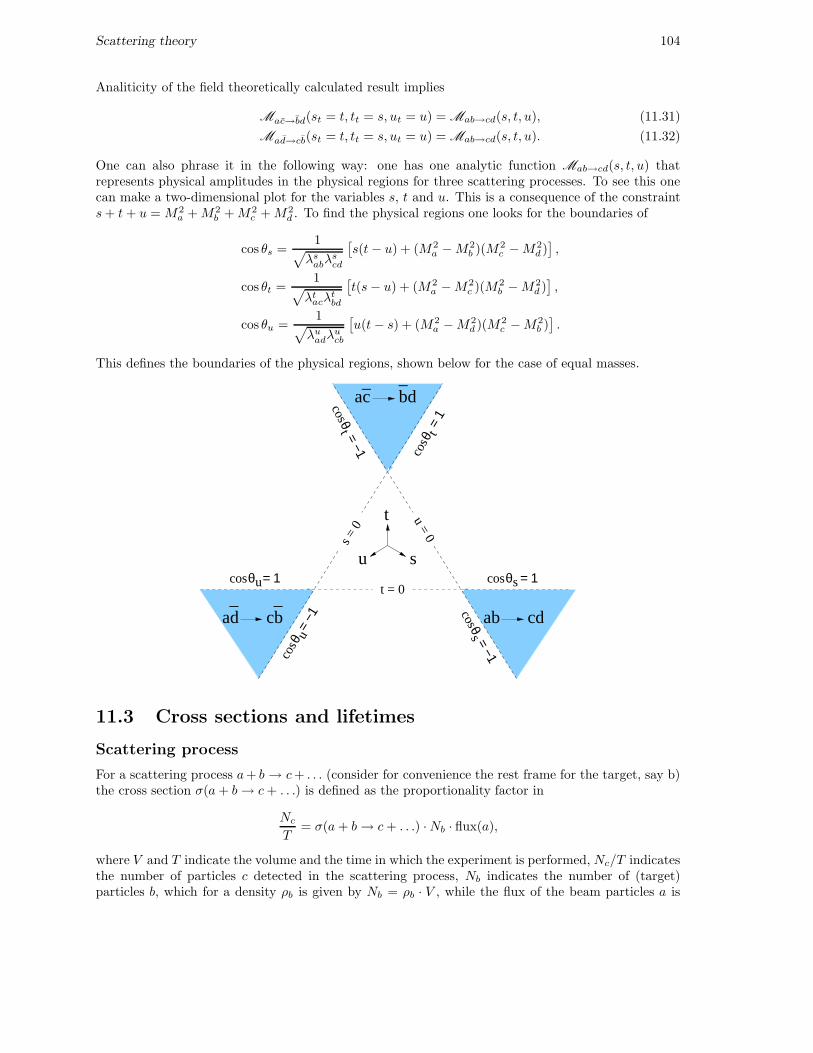
Scattering theory 104
Analiticity of the field theoretically calculated result implies
Mac→bd(st = t, tt = s, ut = u) = Mab→cd(s, t, u), (11.31)
Mad→cb(st = t, tt = s, ut = u) = Mab→cd(s, t, u). (11.32)
One can also phrase it in the following way: one has one analytic function Mab→cd(s, t, u) thatrepresents physical amplitudes in the physical regions for three scattering processes. To see this onecan make a two-dimensional plot for the variables s, t and u. This is a consequence of the constraints+ t+ u = M2
a +M2b +M2
c +M2d . To find the physical regions one looks for the boundaries of
cos θs =1
√λs
abλscd
[s(t− u) + (M2
a −M2b )(M2
c −M2d )],
cos θt =1
√λt
acλtbd
[t(s− u) + (M2
a −M2c )(M2
b −M2d )],
cos θu =1
√λu
adλucb
[u(t− s) + (M2
a −M2d )(M2
c −M2b )].
This defines the boundaries of the physical regions, shown below for the case of equal masses.
ac bd _ _
cb ad __
ab cd
cos θu= 1 cos θs= 1t = 0
cos θ u
= −1 cos θs = −1
cos θt = −1 cos θ t
= 1
s
t
u
s =
0
u = 0
11.3 Cross sections and lifetimes
Scattering process
For a scattering process a+ b → c+ . . . (consider for convenience the rest frame for the target, say b)the cross section σ(a+ b→ c+ . . .) is defined as the proportionality factor in
Nc
T= σ(a+ b→ c+ . . .) ·Nb · flux(a),
where V and T indicate the volume and the time in which the experiment is performed, Nc/T indicatesthe number of particles c detected in the scattering process, Nb indicates the number of (target)particles b, which for a density ρb is given by Nb = ρb · V , while the flux of the beam particles a is
Scattering theory 105
flux(a) = ρa ·vtrfa . The proportionality factor has the dimension of area and is called the cross section,
i.e.
σ =N
T · V1
ρaρb vtrfa
. (11.33)
Although this at first sight does not look covariant, it is. N and T · V are covariant. Using ρtrfa =
ρ(0)a · γa = ρ
(0)a ·Elab
a /ma (where ρ(0)a is the rest frame density) and vlab
a = plaba /Elab
a we have
ρaρb vtrfa =
ρ(0)a ρ
(0)b
4mamb2√
λab
or with ρ(0)a = 2ma,
σ =1
2√λab
N
T · V . (11.34)
Decay of particles
For the decay of particle a one has macroscopically
dN
dt= −ΓN, (11.35)
i.e. the amount of decaying particles is proportional to the number of particles with proportionalityfactor the em decay width Γ. From the solution
N(t) = N(0) e−Γ t (11.36)
one knows that the decay time τ = 1/Γ. Microscopically one has
Ndecay
T= Na · Γ
or
Γ =N
T · V1
ρa. (11.37)
This quantity is not covariant, as expected. The decay time for moving particles τ is related to thedecay time in the rest frame of that particle (the proper decay time τ0) by τ = γ τ0. For the (proper)decay width one thus has
Γ0 =1
2ma
N
T · V . (11.38)
Fermi’s Golden Rule
In both the scattering cross section and the decay constant the quantity N/TV appears. For this weemploy in essence Fermi’s Golden rule stating that when the S-matrix element is written as
Sfi = δfi − (2π)4 δ4(Pi − Pf ) iMfi (11.39)
(in which we can calculate −iMfi using Feynman diagrams), the number of scattered or decayedparticles is given by
N =∣∣(2π)4 δ4(Pi − Pf ) iMfi
∣∣2dR(p1, . . . , pn). (11.40)
One of the δ functions can be rewritten as T · V (remember the normalization of plane waves),
∣∣(2π)4 δ4(Pi − Pf )
∣∣2
= (2π)4 δ4(Pi − Pf )
∫
V,T
d4x ei(Pi−Pf )·x
= (2π)4 δ4(Pi − Pf )
∫
V,T
d4x = V · T (2π)4 δ4(Pi − Pf ).
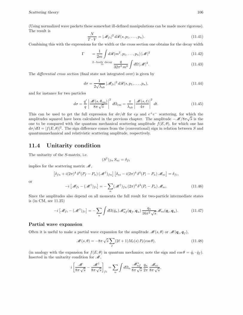
Scattering theory 106
(Using normalized wave packets these somewhat ill-defined manipulations can be made more rigorous).The result is
N
T · V = |Mfi|2 dR(s, p1, . . . , pn). (11.41)
Combining this with the expressions for the width or the cross section one obtains for the decay width
Γ =1
2m
∫
dR(m2, p1, . . . , pn) |M |2 (11.42)
2−body decay=
q
32π2m2
∫
dΩ |M |2. (11.43)
The differential cross section (final state not integrated over) is given by
dσ =1
2√λab
|Mfi|2 dR(s, p1, . . . , pn), (11.44)
and for instance for two particles
dσ =q′
q
∣∣∣∣
M (s, θcm)
8π√s
∣∣∣∣
2
dΩcm =π
λab
∣∣∣∣
M (s, t)
4π
∣∣∣∣
2
dt. (11.45)
This can be used to get the full expression for dσ/dt for eµ and e+e− scattering, for which theamplitudes squared have been calculated in the previous chapter. The amplitude −M /8π
√s is the
one to be compared with the quantum mechanical scattering amplitude f(E, θ), for which one hasdσ/dΩ = |f(E, θ)|2. The sign difference comes from the (conventional) sign in relation between S andquantummechanical and relativistic scattering amplitude, respectively.
11.4 Unitarity condition
The unitarity of the S-matrix, i.e.(S†)fn Sni = δfi
implies for the scattering matrix M ,[δfn + i(2π)4 δ4(Pf − Pn) (M †)fn
] [δni − i(2π)4 δ4(Pi − Pn)Mni
]= δfi,
or−i[Mfi − (M †)fi
]= −
∑
n
(M †)fn (2π)4 δ4(Pi − Pn)Mni. (11.46)
Since the amplitudes also depend on all momenta the full result for two-particle intermediate statesis (in CM, see 11.25)
−i[Mfi − (M †)fi
]= −
∑
n
∫
dΩ(qn)M ∗nf (qf , qn)
qn16π2
√sMni(qi, qn). (11.47)
Partial wave expansion
Often it is useful to make a partial wave expansion for the amplitude M (s, θ) or M (qi, qf ),
M (s, θ) = −8π√s∑
ℓ
(2ℓ+ 1)Mℓ(s)Pℓ(cos θ), (11.48)
(in analogy with the expansion for f(E, θ) in quantum mechanics; note the sign and cos θ = qi · qf ).Inserted in the unitarity condition for M ,
i
[M
8π√s− M †
8π√s
]
fi
=∑
n
∫
dΩn
M ∗nf
8π√s
qn2π
Mni
8π√s,
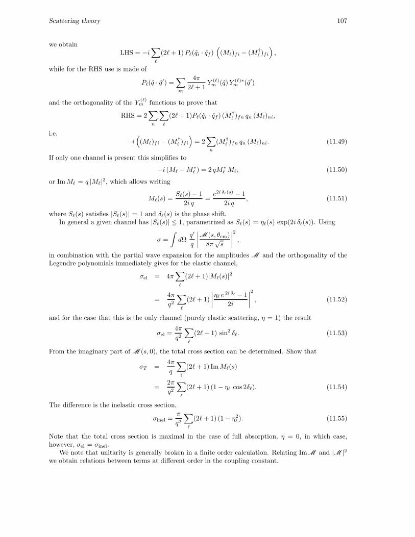
Scattering theory 107
we obtainLHS = −i
∑
ℓ
(2ℓ+ 1)Pℓ(qi · qf )(
(Mℓ)fi − (M †ℓ )fi
)
,
while for the RHS use is made of
Pℓ(q · q′) =∑
m
4π
2ℓ+ 1Y (ℓ)
m (q)Y (ℓ)∗m (q′)
and the orthogonality of the Y(ℓ)m functions to prove that
RHS = 2∑
n
∑
ℓ
(2ℓ+ 1)Pℓ(qi · qf ) (M †ℓ )fn qn (Mℓ)ni,
i.e.−i(
(Mℓ)fi − (M †ℓ )fi
)
= 2∑
n
(M †ℓ )fn qn (Mℓ)ni. (11.49)
If only one channel is present this simplifies to
−i (Mℓ −M∗ℓ ) = 2 qM∗ℓ Mℓ, (11.50)
or ImMℓ = q |Mℓ|2, which allows writing
Mℓ(s) =Sℓ(s) − 1
2i q=e2i δℓ(s) − 1
2i q, (11.51)
where Sℓ(s) satisfies |Sℓ(s)| = 1 and δℓ(s) is the phase shift.In general a given channel has |Sℓ(s)| ≤ 1, parametrized as Sℓ(s) = ηℓ(s) exp(2i δℓ(s)). Using
σ =
∫
dΩq′
q
∣∣∣∣
M (s, θcm)
8π√s
∣∣∣∣
2
,
in combination with the partial wave expansion for the amplitudes M and the orthogonality of theLegendre polynomials immediately gives for the elastic channel,
σel = 4π∑
ℓ
(2ℓ+ 1)|Mℓ(s)|2
=4π
q2
∑
ℓ
(2ℓ+ 1)
∣∣∣∣
ηℓ e2i δℓ − 1
2i
∣∣∣∣
2
, (11.52)
and for the case that this is the only channel (purely elastic scattering, η = 1) the result
σel =4π
q2
∑
ℓ
(2ℓ+ 1) sin2 δℓ. (11.53)
From the imaginary part of M (s, 0), the total cross section can be determined. Show that
σT =4π
q
∑
ℓ
(2ℓ+ 1) ImMℓ(s)
=2π
q2
∑
ℓ
(2ℓ+ 1) (1 − ηℓ cos 2δℓ). (11.54)
The difference is the inelastic cross section,
σinel =π
q2
∑
ℓ
(2ℓ+ 1) (1 − η2ℓ ). (11.55)
Note that the total cross section is maximal in the case of full absorption, η = 0, in which case,however, σel = σinel.
We note that unitarity is generally broken in a finite order calculation. Relating ImM and |M |2we obtain relations between terms at different order in the coupling constant.
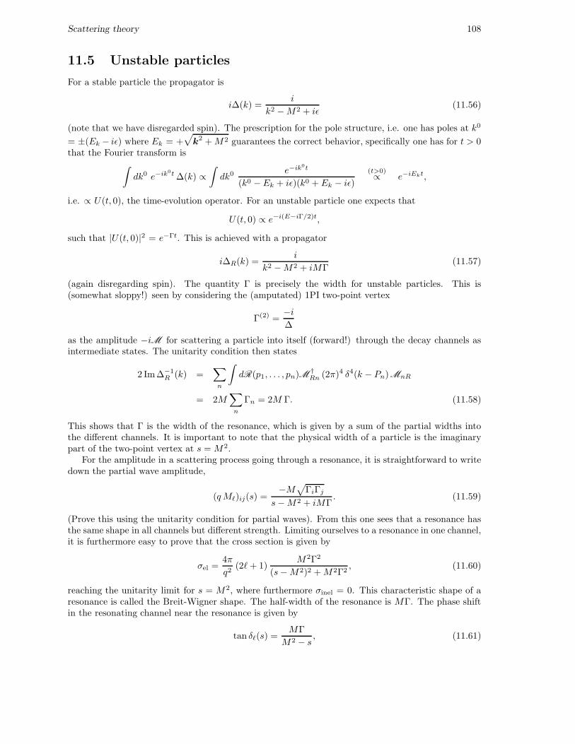
Scattering theory 108
11.5 Unstable particles
For a stable particle the propagator is
i∆(k) =i
k2 −M2 + iǫ(11.56)
(note that we have disregarded spin). The prescription for the pole structure, i.e. one has poles at k0
= ±(Ek − iǫ) where Ek = +√
k2 +M2 guarantees the correct behavior, specifically one has for t > 0that the Fourier transform is
∫
dk0 e−ik0t ∆(k) ∝∫
dk0 e−ik0t
(k0 − Ek + iǫ)(k0 + Ek − iǫ)
(t>0)∝ e−iEkt,
i.e. ∝ U(t, 0), the time-evolution operator. For an unstable particle one expects that
U(t, 0) ∝ e−i(E−iΓ/2)t,
such that |U(t, 0)|2 = e−Γt. This is achieved with a propagator
i∆R(k) =i
k2 −M2 + iMΓ(11.57)
(again disregarding spin). The quantity Γ is precisely the width for unstable particles. This is(somewhat sloppy!) seen by considering the (amputated) 1PI two-point vertex
Γ(2) =−i∆
as the amplitude −iM for scattering a particle into itself (forward!) through the decay channels asintermediate states. The unitarity condition then states
2 Im∆−1R (k) =
∑
n
∫
dR(p1, . . . , pn)M †Rn (2π)4 δ4(k − Pn)MnR
= 2M∑
n
Γn = 2M Γ. (11.58)
This shows that Γ is the width of the resonance, which is given by a sum of the partial widths intothe different channels. It is important to note that the physical width of a particle is the imaginarypart of the two-point vertex at s = M2.
For the amplitude in a scattering process going through a resonance, it is straightforward to writedown the partial wave amplitude,
(qMℓ)ij(s) =−M
√ΓiΓj
s−M2 + iMΓ. (11.59)
(Prove this using the unitarity condition for partial waves). From this one sees that a resonance hasthe same shape in all channels but different strength. Limiting ourselves to a resonance in one channel,it is furthermore easy to prove that the cross section is given by
σel =4π
q2(2ℓ+ 1)
M2Γ2
(s−M2)2 +M2Γ2, (11.60)
reaching the unitarity limit for s = M2, where furthermore σinel = 0. This characteristic shape of aresonance is called the Breit-Wigner shape. The half-width of the resonance is MΓ. The phase shiftin the resonating channel near the resonance is given by
tan δℓ(s) =MΓ
M2 − s, (11.61)
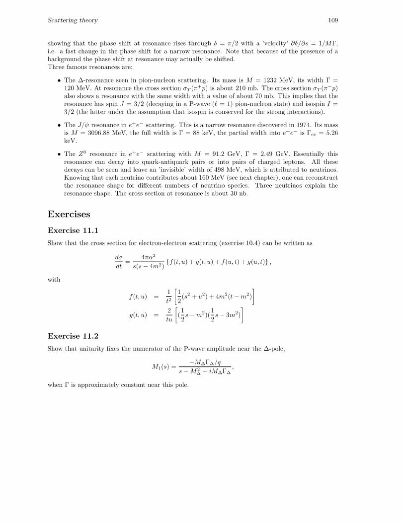
Scattering theory 109
showing that the phase shift at resonance rises through δ = π/2 with a ’velocity’ ∂δ/∂s = 1/MΓ,i.e. a fast change in the phase shift for a narrow resonance. Note that because of the presence of abackground the phase shift at resonance may actually be shifted.Three famous resonances are:
• The ∆-resonance seen in pion-nucleon scattering. Its mass is M = 1232 MeV, its width Γ =120 MeV. At resonance the cross section σT (π+p) is about 210 mb. The cross section σT (π−p)also shows a resonance with the same width with a value of about 70 mb. This implies that theresonance has spin J = 3/2 (decaying in a P-wave (ℓ = 1) pion-nucleon state) and isospin I =3/2 (the latter under the assumption that isospin is conserved for the strong interactions).
• The J/ψ resonance in e+e− scattering. This is a narrow resonance discovered in 1974. Its massis M = 3096.88 MeV, the full width is Γ = 88 keV, the partial width into e+e− is Γee = 5.26keV.
• The Z0 resonance in e+e− scattering with M = 91.2 GeV, Γ = 2.49 GeV. Essentially thisresonance can decay into quark-antiquark pairs or into pairs of charged leptons. All thesedecays can be seen and leave an ’invisible’ width of 498 MeV, which is attributed to neutrinos.Knowing that each neutrino contributes about 160 MeV (see next chapter), one can reconstructthe resonance shape for different numbers of neutrino species. Three neutrinos explain theresonance shape. The cross section at resonance is about 30 nb.
Exercises
Exercise 11.1
Show that the cross section for electron-electron scattering (exercise 10.4) can be written as
dσ
dt=
4πα2
s(s− 4m2)f(t, u) + g(t, u) + f(u, t) + g(u, t) ,
with
f(t, u) =1
t2
[1
2(s2 + u2) + 4m2(t−m2)
]
g(t, u) =2
tu
[
(1
2s−m2)(
1
2s− 3m2)
]
Exercise 11.2
Show that unitarity fixes the numerator of the P-wave amplitude near the ∆-pole,
M1(s) =−M∆Γ∆/q
s−M2∆ + iM∆Γ∆
,
when Γ is approximately constant near this pole.
Chapter 12
The standard model
12.1 Non-abelian gauge theories
In chapter 10 we have considered quantum electrodynamics as an example of a gauge theory. The pho-ton field Aµ was introduced as to render the lagrangian invariant under local gauge transformations.The extension to non-abelian gauge theories is straightforward. The symmetry group is a Lie-groupG generated by generators Ta, which satisfy commutation relations
[Ta, Tb] = i cabc Tc, (12.1)
with cabc known as the structure constants of the group. For a compact Lie-group they are antisym-metric in the three indices. In an abelian group the structure constants would be zero (for instancethe trivial example of U(1)). Consider a field transforming under the group,
φ(x) −→ ei θa(x)Laφ(x)inf= (1 + i θa(x)La)φ(x) (12.2)
where La is a representation matrix for the representation to which φ belongs, i.e. for a three-component field ~φ under an SO(3) or SU(2) symmetry transformation,
~φ −→ ei ~θ·~L~φinf= ~φ− ~θ × ~φ. (12.3)
The complication arises (as in the abelian case) when one considers for a lagrangian densityL (φ, ∂µφ) the behavior of ∂µφ under a local gauge transformation, U(θ) = ei θa(x)La ,
φ(x) −→ U(θ)φ(x), (12.4)
∂µφ(x) −→ U(θ)∂µφ(x) + (∂µU(θ))φ(x). (12.5)
Introducing as many gauge fields as there are generators in the group, which are conveniently combinedin the matrix valued field Wµ = W a
µLa, one defines
Dµφ(x) ≡(∂µ − igWµ
)φ(x), (12.6)
and one obtains after transformation
Dµφ(x) −→ U(θ)∂µφ(x) + (∂µU(θ))φ(x) − igW ′µ U(θ)φ(x).
Requiring that Dµφ transforms as Dµφ → U(θ)Dµφ (or Dµ → U(θ)DµU−1(θ)) gives
Dµφ(x) −→ U(θ)∂µφ(x) − ig U(θ)W µφ(x),
110
The standard model 111
which implies
W ′µ = U(θ)Wµ U−1(θ) − i
g(∂µU(θ))U−1(θ), (12.7)
or infinitesimal
W ′aµ = W aµ − cabcθ
bW cµ +
1
g∂µθ
a = W aµ +
1
gDµθ
a.
It is necessary to introduce the free lagrangian density for the gauge fields just like the term−(1/4)FµνF
µν in QED. For abelian fields Fµν = ∂µAν − ∂νAµ = (i/g)[Dµ, Dν ] is gauge invariant. Inthe nonabelian case ∂µW
aν − ∂νW
aµ does not provide a gauge invariant candidate for Gµν = Ga
µνLa,as can be checked easily. Generalizing the expression in terms of the covariant derivatives, provides agauge invariant definition for Gµν . We have
Gµν =i
g[Dµ, Dν ] = ∂µW ν − ∂νWµ − ig [Wµ,W ν ], (12.8)
with for the explicit fieldsGa
µν = ∂µWaν − ∂νW
aµ + g cabcW
bµW
cν , (12.9)
transforming likeGµν → U(θ)Gµν U
−1(θ). (12.10)
The gauge-invariant lagrangian density is now constructed as
L (φ, ∂µφ) −→ L (φ,Dµφ) − 1
2TrGµνG
µν = L (φ,Dµφ) − 1
4Ga
µνGµν a (12.11)
with the standard normalization Tr(LaLb) = 12δab. Note that the gauge fields must be massless, as a
mass term ∝M2WW a
µWµ a would break gauge invariance.
QCD, an example of a nonabelian gauge theory
As an example of a nonabelian gauge theory consider quantum chromodynamics (QCD), the theorydescribing the interactions of the colored quarks. The existence of an extra degree of freedom foreach species of quarks is evident for several reasons, e.g. the necessity to have an antisymmetric wavefunction for the ∆++ particle consisting of three up quarks (each with charge +(2/3)e). With thequarks belonging to the fundamental (three-dimensional) representation of SU(3)C , i.e. having threecomponents in color space
ψ =
ψr
ψg
ψb
,
the wave function of the baryons (such as nucleons and deltas) form a singlet under SU(3)C ,
|color〉 =1√6
(|rgb〉 − |grb〉 + |gbr〉 − |bgr〉 + |brg〉 − |rbg〉) . (12.12)
The nonabelian gauge theory that is obtained by making the ’free’ quark lagrangian, for one specificspecies (flavor) of quarks just the Dirac lagrangian for an elementary fermion,
L = i ψ/∂ψ −mψψ,
invariant under local SU(3)C transformations has proven to be a good candidate for the microscopictheory of the strong interactions. The representation matrices for the quarks and antiquarks in thefundamental representation are given by
Fa =λa
2for quarks,
Fa = −λ∗a
2for antiquarks,
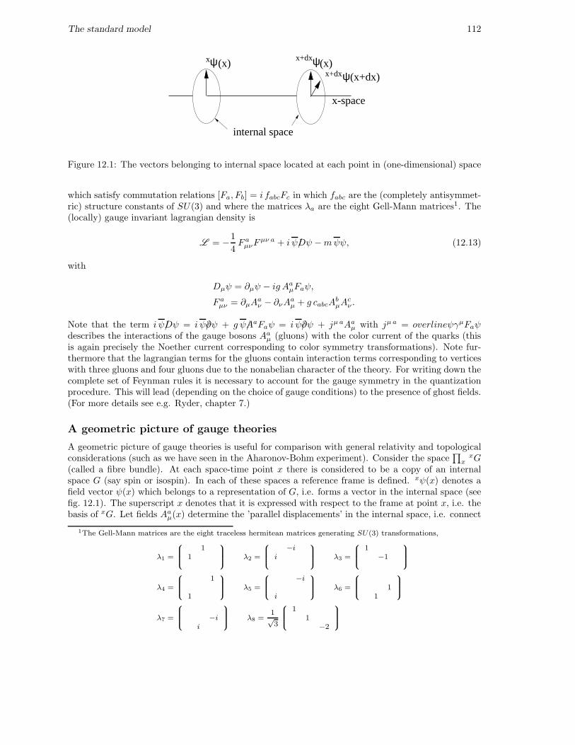
The standard model 112
internal space
ψx (x) ψx+dx(x)
x+dxψ(x+dx)
x-space
Figure 12.1: The vectors belonging to internal space located at each point in (one-dimensional) space
which satisfy commutation relations [Fa, Fb] = i fabcFc in which fabc are the (completely antisymmet-ric) structure constants of SU(3) and where the matrices λa are the eight Gell-Mann matrices1. The(locally) gauge invariant lagrangian density is
L = −1
4F a
µνFµν a + i ψ/Dψ −mψψ, (12.13)
with
Dµψ = ∂µψ − ig AaµFaψ,
F aµν = ∂µA
aν − ∂νA
aµ + g cabcA
bµA
cν .
Note that the term i ψ/Dψ = i ψ/∂ψ + g ψ/AaFaψ = i ψ/∂ψ + jµ aAaµ with jµ a = overlineψγµFaψ
describes the interactions of the gauge bosons Aaµ (gluons) with the color current of the quarks (this
is again precisely the Noether current corresponding to color symmetry transformations). Note fur-thermore that the lagrangian terms for the gluons contain interaction terms corresponding to verticeswith three gluons and four gluons due to the nonabelian character of the theory. For writing down thecomplete set of Feynman rules it is necessary to account for the gauge symmetry in the quantizationprocedure. This will lead (depending on the choice of gauge conditions) to the presence of ghost fields.(For more details see e.g. Ryder, chapter 7.)
A geometric picture of gauge theories
A geometric picture of gauge theories is useful for comparison with general relativity and topologicalconsiderations (such as we have seen in the Aharonov-Bohm experiment). Consider the space
∏
xxG
(called a fibre bundle). At each space-time point x there is considered to be a copy of an internalspace G (say spin or isospin). In each of these spaces a reference frame is defined. xψ(x) denotes afield vector ψ(x) which belongs to a representation of G, i.e. forms a vector in the internal space (seefig. 12.1). The superscript x denotes that it is expressed with respect to the frame at point x, i.e. thebasis of xG. Let fields Aa
µ(x) determine the ’parallel displacements’ in the internal space, i.e. connect
1The Gell-Mann matrices are the eight traceless hermitean matrices generating SU(3) transformations,
λ1 =
8
>
>
>
>
>
:
11
9
>
>
>
>
>
;
λ2 =
8
>
>
>
>
>
:
−ii
9
>
>
>
>
>
;
λ3 =
8
>
>
>
>
>
:
1−1
9
>
>
>
>
>
;
λ4 =
8
>
>
>
>
>
:
1
1
9
>
>
>
>
>
;
λ5 =
8
>
>
>
>
>
:
−i
i
9
>
>
>
>
>
;
λ6 =
8
>
>
>
>
>
:
11
9
>
>
>
>
>
;
λ7 =
8
>
>
>
>
>
:
−ii
9
>
>
>
>
>
;
λ8 =1√3
8
>
>
>
>
>
:
11
−2
9
>
>
>
>
>
;

The standard model 113
the basis for xG and x+dxG,
x+dxψ(x) =(1 + ig dxµ Aa
µ(x)Ta
)xψ(x) (12.14)
=(1 + ig dxµ Aµ(x)
)xψ(x), (12.15)
which connects two identical vectors, but expresses them with respect to different bases.If there is a ’true’ difference in the vector ψ(x) and ψ(x + dx) it is denoted with the covariant
derivative connecting the vectors expressed with respect to the same basis, i.e.
x+dxψ(x+ dx) =(1 + dxµ Dµ
)x+dxψ(x), (12.16)
which in the presence of the ’connection’ Aµ differs from the total change between xψ(x) and x+dxψ(x+dx),
x+dxψ(x+ dx) = (1 + dxµ ∂µ)xψ(x). (12.17)
The three equations given so far immediately give
Dµ = ∂µ − ig Aµ(x). (12.18)
We note that local gauge invariance requires that we can modify all local systems with a (local) unitarytransformation S(x). The relation in Eq. 12.16, should be independent of such transformations,requiring that the ’connection’ Aµ(x) is such that Dµ → S(x)DµS
−1(x).A ’constant’ vector that only rotates because of the arbitrary definitions of local frames satisfies
Dµ ψ(x) = 0, i.e.[∂µ − ig Aµ(x)
]ψ(x) = 0
or considering a path xµ(s) from a fixed origin (0) to point x,
dxµ
ds
[∂µ − ig Aµ(x(s))
]ψ(x) = 0,
which is solved by
dψ(s)
ds= ig Aµ(s)ψ(s)
dxµ
ds,
ψ(s) = P exp
(
ig
∫ s
0
ds′dxµ
ds′Aµ(s′)
)
ψ(0),
which is the path-ordered integral denoted
ψ(x) = P eigR
Pdxµ Aµ(x)ψ(0). (12.19)
This gives rise to a (path dependent) phase in each point.In principle such a phase in a given point is not observable. However, if two different paths to the
same point give different phases the effects can be observed. What is this physical effect by which the’connection’ Aµ can be observed? For this consider the phase around a closed loop,
dy-dy
-dx
dx
µ
µ
µ
µ
For the constant vector, it is given by
ψ(x) = (1 − i dyρDρ)(1 − i dxσDσ)(1 + i dyνDν)(1 + i dxµDµ)ψ(x)
=(1 + dxµdyν [Dµ, Dν ]
)ψ(x)
=(1 − ig dσµν Gµν
)ψ(x),
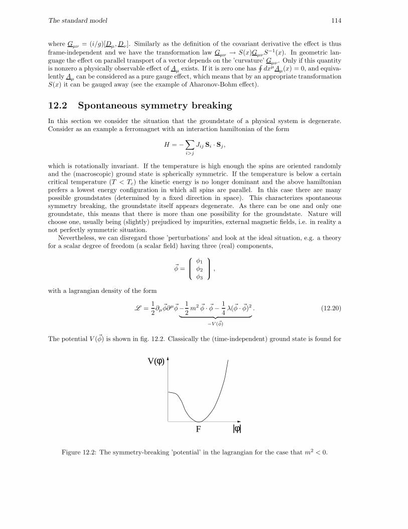
The standard model 114
where Gµν = (i/g)[Dµ, Dν ]. Similarly as the definition of the covariant derivative the effect is thus
frame-independent and we have the transformation law Gµν → S(x)GµνS−1(x). In geometric lan-
guage the effect on parallel transport of a vector depends on the ’curvature’ Gµν . Only if this quantityis nonzero a physically observable effect of Aµ exists. If it is zero one has
∮dxµAµ(x) = 0, and equiva-
lently Aµ can be considered as a pure gauge effect, which means that by an appropriate transformationS(x) it can be gauged away (see the example of Aharonov-Bohm effect).
12.2 Spontaneous symmetry breaking
In this section we consider the situation that the groundstate of a physical system is degenerate.Consider as an example a ferromagnet with an interaction hamiltonian of the form
H = −∑
i>j
Jij Si · Sj ,
which is rotationally invariant. If the temperature is high enough the spins are oriented randomlyand the (macroscopic) ground state is spherically symmetric. If the temperature is below a certaincritical temperature (T < Tc) the kinetic energy is no longer dominant and the above hamiltonianprefers a lowest energy configuration in which all spins are parallel. In this case there are manypossible groundstates (determined by a fixed direction in space). This characterizes spontaneoussymmetry breaking, the groundstate itself appears degenerate. As there can be one and only onegroundstate, this means that there is more than one possibility for the groundstate. Nature willchoose one, usually being (slightly) prejudiced by impurities, external magnetic fields, i.e. in reality anot perfectly symmetric situation.
Nevertheless, we can disregard those ’perturbations’ and look at the ideal situation, e.g. a theoryfor a scalar degree of freedom (a scalar field) having three (real) components,
~φ =
φ1
φ2
φ3
,
with a lagrangian density of the form
L =1
2∂µ~φ∂µ~φ−1
2m2 ~φ · ~φ− 1
4λ(~φ · ~φ)2
︸ ︷︷ ︸
−V (~φ)
. (12.20)
The potential V (~φ) is shown in fig. 12.2. Classically the (time-independent) ground state is found for
V( )φ
|φ|F
Figure 12.2: The symmetry-breaking ’potential’ in the lagrangian for the case that m2 < 0.
The standard model 115
a constant field (∇~φ = 0) and the condition
∂V
∂~φ
∣∣∣∣ϕc
= 0 −→ ~ϕc · ~ϕc = 0 or ~ϕc · ~ϕc = −m2
λ≡ F 2,
the latter only forming a minimum for m2 < 0. In this situation one speaks of spontaneous symmetrybreaking. The classical groundstate appears degenerate. Any constant field ϕc with ’length’ |~φ| = F isa possible groundstate. The presence of a nonzero value for the classical groundstate value of the fieldwill have an effect when the field is quantized. A quantum field theory has only one nondegenerategroundstate |0〉. Writing the field ~φ as a sum of a classical and a quantum field, ~φ = ~ϕc + ~φquantumwhere for the (operator-valued) coefficients in the quantum field one wants 〈0|c† = c|0〉 = 0, so onehas
〈0|φquantum|0〉 = 0 and 〈0|~φ|0〉 = ~ϕc. (12.21)
Stability of the action requires the classical groundstate ~ϕc to have a well-defined value (which canbe nonzero), while the quadratic terms must correspond with non-negative masses. In the case ofdegeneracy, therefore a choice must be made, say
〈0|~φ|0〉 =
00F
. (12.22)
The situation now is the following. The original lagrangian contained an SO(3) invariance under(length conserving) rotations among the three fields, while the lagrangian including the nonzerogroundstate expectation value chosen by nature, has less symmetry. It is only invariant under ro-tations around the 3-axis.
It is appropriate to redefine the field as
~φ =
ϕ1
ϕ2
F + η
, (12.23)
such that 〈0|ϕ1|0〉 = 〈0|ϕ2|0〉 = 〈0|η|0〉 = 0. The field along the third axis plays a special role becauseof the choice of the vacuum expectation value. In order to see the consequences for the particlespectrum of the theory we construct the lagrangian in terms of the fields ϕ1, ϕ2 and η. It is sufficientto do this to second order in the fields as the higher (cubic, etc.) terms constitute interaction terms.The result is
L =1
2(∂µϕ1)
2 +1
2(∂µϕ2)
2 +1
2(∂µη)
2 − 1
2m2 (ϕ2
1 + ϕ22)
−1
2m2 (F + η)2 − 1
4λ (ϕ2
1 + ϕ22 + F 2 + η2 + 2Fη)2 (12.24)
=1
2(∂µϕ1)
2 +1
2(∂µϕ2)
2 +1
2(∂µη)
2 +m2 η2 + . . . . (12.25)
Therefore there are 2 massless scalar particles, corresponding to the number of broken generators (inthis case rotations around 1 and 2 axis) and 1 massive scalar particle with mass m2
η = −2m2. Themassless particles are called Goldstone bosons.
Realization of symmetries
In this section we want to discuss a bit more formal the two possible ways that a symmetry can beimplemented. They are known as the Weyl mode or the Goldstone mode:
Weyl mode. In this mode the lagrangian and the vacuum are both invariant under a set of symmetrytransformations generated by Qa, i.e. for the vacuum Qa|0〉 = 0. In this case the spectrum is described
The standard model 116
by degenerate representations of the symmetry group. Known examples are rotational symmetry andthe fact that the the spectrum shows multiplets labeled by angular momentum ℓ (with memberslabeled by m). The generators Qa (in that case the rotation operators Lz, Lx and Ly or instead of thelatter two L+ and L−) are used to label the multiplet members or transform them into one another.A bit more formal, if the generators Qa generate a symmetry, i.e. [Qa, H ] = 0, and |a〉 and |a′〉 belongto the same multiplet (there is a Qa such that |a′〉 = Qa|a〉) then H |a〉 = Ea|a〉 implies that H |a′〉 =Ea|a′〉, i.e. a and a′ are degenerate states.
Goldstone mode. In this mode the lagrangian is invariant but Qa|0〉 6= 0 for a number of generators.This means that they are operators that create states from the vacuum, denoted |πa(k)〉. As thegenerators for a symmetry are precisely the zero-components of a conserved current Ja
µ(x) integratedover space, there must be a nonzero expectation value 〈0|Ja
µ(x)|πa(k)〉. Using translation invarianceand as kµ is the only four vector on which this matrix element could depend one may write
〈0|Jaµ(x)|πb(k)〉 = fπ kµ e
i k·x δab (fπ 6= 0) (12.26)
for all the states labeled by a corresponding to ’broken’ generators. Taking the derivative,
〈0|∂µJaµ(x)|πb(k)〉 = fπ k
2 ei k·x δab = fπ m2πa ei k·x δab. (12.27)
If the transformations in the lagrangian give rise to a symmetry the Noether currents are conserved,∂µJa
µ = 0, irrespective of the fact if they annihilate the vacuum, and one must have mπa = 0, i.e. amassless Goldstone boson for each ’broken’ generator. Note that for the fields πa(x) one would havethe relation 〈0|πa(x)|πa(k)〉 = ei k·x, suggesting the stronger relation ∂µJa
µ(x) = fπ m2πa πa(x).
Chiral symmetry
An example of spontaneous symmetry breaking is chiral symmetry breaking in QCD. Neglecting atthis point the local color symmetry, the lagrangian for the quarks consists of the free Dirac lagrangianfor each of the types of quarks, called flavors. Including a sum over the different flavors (up, down,strange, etc.) one can write
L = ψ(i/∂ −M)ψ, (12.28)
where ψ is extended to a vector in flavor space and M is a diagonal matrix,
ψ =
ψu
ψd
...
, M =
mu
md
. . .
(12.29)
(Note that each of the entries in the vector for ψ is a 4-component Dirac spinor). This lagrangiandensity then is invariant under unitary (vector) transformations in the flavor space,
ψ −→ ei ~α·~Tψ, (12.30)
which for instance including only two flavors form an SU(2)V symmetry (isospin symmetry) gen-
erated by the Pauli matrices, ~T = ~τ/2. The conserved currents corresponding to this symmetrytransformation are found directly using Noether’s theorem (see chapter 6),
~V µ = ψγµ ~Tψ. (12.31)
Using the Dirac equation, it is easy to see that one gets
∂µ~V µ = i ψ [M, ~T ]ψ. (12.32)

The standard model 117
Furthermore ∂µ~V µ = 0 ⇐⇒ [M, ~T ] = 0. From group theory (Schur’s theorem) one knows that the
latter can only be true, if in flavor space M is proportional to the unit matrix, M = m ·1. I.e. SU(2)V
(isospin) symmetry is good if the up and down quark masses are identical. This situation, both arevery small, is what happens in the real world. This symmetry is realized in the Weyl mode withthe spectrum of QCD showing an almost perfect isospin symmetry, e.g. a doublet (isospin 1/2) ofnucleons, proton and neutron, with almost degenerate masses (Mp = 938.3 MeV/c2 and Mn = 939.6MeV/c2), but also a triplet (isospin 1) of pions, etc.
There exists another set of symmetry transformations, socalled axial vector transformations,
ψ −→ ei ~α·~Tγ5ψ, (12.33)
which for instance including only two flavors form SU(2)A transformations generated by the Pauli
matrices, ~Tγ5 = ~τγ5/2. Note that these transformations also work on the spinor indices. The currentscorresponding to this symmetry transformation are again found using Noether’s theorem,
~Aµ = ψγµ ~Tγ5ψ. (12.34)
Using the Dirac equation, it is easy to see that one gets
∂µ~Aµ = i ψ M, ~T γ5 ψ. (12.35)
In this case ∂µ~Aµ = 0 will be true if the quarks have zero mass, which is approximately true for the up
and down quarks. Therefore the world of up and down quarks describing pions, nucleons and atomicnuclei has not only an isospin or vector symmetry SU(2)V but also an axial vector symmetry SU(2)A.This combined symmetry is what one calls chiral symmetry.
That the massless theory has this symmetry can also be seen by writing it down for the socalledlefthanded and righthanded fermions, ψR/L = 1
2 (1 ± γ5)ψ, in terms of which the Dirac lagrangiandensity looks like
L = i ψL/∂ψL + i ψR/∂ψR − ψRMψL − ψLMψR. (12.36)
If the mass is zero the lagrangian is split into two disjunct parts for L and R showing that there isa direct product SU(2)L ⊗ SU(2)R symmetry, generated by ~TR/L = 1
2 (1 ± γ5)~T , which is equivalentto the V-A symmetry. This symmetry, however, is by nature not realized in the Weyl mode. Howcan we see this. The chiral fields ψR and ψL are transformed into each other under parity. Thereforerealization in the Weyl mode would require that all particles come double with positive and negativeparity, or, stated equivalently, parity would not play a role in the world. We know that mesons andbaryons (such as the nucleons) have a well-defined parity that is conserved.
The conclusion is that the original symmetry of the lagrangian is spontaneously broken and as thevector part of the symmetry is the well-known isospin symmetry, nature has choosen the path
SU(2)L ⊗ SU(2)R =⇒ SU(2)V ,
i.e. the lagrangian density is invariant under left (L) and right (R) rotations independently, while thegroundstate is only invariant under isospin rotations (R = L). From the number of broken generatorsit is clear that one expects three massless Goldstone bosons, for which the field (according to thediscussion above) has the same behavior under parity, etc. as the quantity ∂µA
µ(x), i.e. (leavingout the flavor structure) the same as ψγ5ψ, i.e. behaves as a pseudoscalar particle (spin zero, parityminus). In the real world, where the quark masses are not completely zero, chiral symmetry is notperfect. Still the basic fact that the generators acting on the vacuum give a nonzero result (i.e. fπ 6= 0remains, but the fact that the symmetry is not perfect and the right hand side of Eq. 12.35 is nonzero,gives also rise to a nonzero mass for the Goldstone bosons according to Eq. 12.27. The Goldstonebosons of QCD are the pions for which fπ = 93 MeV and which have a mass of mπ ≈ 138 MeV/c2,much smaller than any of the other mesons or baryons.
The standard model 118
12.3 The Higgs mechanism
The Higgs mechanism occurs when spontaneous symmetry breaking happens in a gauge theory wheregauge bosons have been introduced in order to assure the local symmetry. Considering the sameexample with rotational symmetry (SO(3)) as for spontaneous symmetry breaking of a scalar field(Higgs field) with three components, made into a gauge theory,
L = −1
4~Gµν · ~Gµν +
1
2Dµ
~φ ·Dµ~φ− V (~φ), (12.37)
whereDµ
~φ = ∂µ~φ− igW a
µLa~φ. (12.38)
Since the explicit (conjugate, in this case three-dimensional) representation (La)ij = −i ǫaij one sees
that the fields ~Wµ and ~Gµν also can be represented as three-component fields,
Dµ~φ = ∂µ
~φ+ g ~Wµ × ~φ, (12.39)
~Gµν = ∂µ~Wν − ∂ν
~Wµ + g ~Wµ × ~Wν . (12.40)
The symmetry is broken in the same way as before and the same choice for the vacuum,
~ϕc = 〈0|~φ|0〉 =
00F
.
is made. The difference comes when we reparametrize the field ~φ. We have the possibility to performlocal gauge transformations. Therefore we can always rotate the field φ into the z-direction in orderto simplify the calculation, i.e.
~φ =
00φ3
=
00
F + η
. (12.41)
Explicitly one then has
Dµ~φ = ∂µ
~φ+ g ~Wµ × ~φ =
gF W 2µ + gW 2
µ η−gF W 1
µ − gW 1µ η
∂µη
,
which gives for the lagrangian density up to quadratic terms
L = −1
4~Gµν · ~Gµν +
1
2Dµ
~φ ·Dµ~φ− 1
2m2~φ · ~φ− λ
4(~φ · ~φ)2
= −1
4(∂µ
~Wν − ∂ν~Wµ) · (∂µ ~W ν − ∂ν ~Wµ) − 1
2g2F 2
(W 1
µWµ 1 +W 2
µWµ 2)
+1
2(∂µη)
2 +m2 η2 + . . . , (12.42)
from which one reads off that the particle content of the theory consists of one massless gauge boson(W 3
µ), two massive bosons (W 1µ and W 2
µ with MW = gF ) and a massive scalar particle (η with m2η =
−2m2. The latter is a spin 0 particle (real scalar field) called a Higgs particle. Note that the numberof massless gauge bosons (in this case one) coincides with the number of generators corresponding tothe remaining symmetry (in this case rotations around the 3-axis), while the number of massive gaugebosons coincides with the number of ’broken’ generators.
One may wonder about the degrees of freedom, as in this case there are no massless Goldstonebosons. Initially there are 3 massless gauge fields (each, like a photon, having two independent spincomponents) and three scalar fields (one degree of freedom each), thus 9 independent degrees offreedom. After symmetry breaking the same number (as expected) comes out, but one has 1 masslessgauge field (2), 2 massive vector fields or spin 1 bosons (2 × 3) and one scalar field (1), again 9 degreesof freedom.
The standard model 119
12.4 The standard model SU(2)W ⊗ U(1)Y
The symmetry ideas discussed before play an essential role in the standard model that describesthe elementary particles, the quarks (up, down, etc.), the leptons (elektrons, muons, neutrinos, etc.)and the gauge bosons responsible for the strong, electromagnetic and weak forces. In the standardmodel one starts with a very simple basic lagrangian for (massless) fermions which exhibits moresymmetry than observed in nature. By introducing gauge fields and breaking the symmetry a morecomplex lagrangian is obtained, that gives a good description of the physical world. The procedure,however, implies certain nontrivial relations between masses and mixing angles that can be testedexperimentally and sofar are in excellent agreement with experiment.
The lagrangian for the leptons consists of three families each containing an elementary fermion(electron e−, muon µ− or tau τ−), its corresponding neutrino (νe, νµ and ντ ) and their antiparticles.As they are massless, left- and righthanded particles, ψR/L = 1
2 (1 ± γ5)ψ decouple. For the neutrinoonly a lefthanded particle (and righthanded antiparticle) exist. Thus
L(f) = i eR/∂eR + i eL/∂eL + i νeL/∂νeL + (µ, τ). (12.43)
One introduces a (weak) SU(2)W symmetry under which eR forms a singlet, while the lefthandedparticles form a doublet, i.e.
L =
νe
eL
with TW =1
2and T 3
W =
+1/2−1/2
andR = eR with TW = 0 and T 3
W = 0.
Thus the lagrangian density isL
(f) = i L/∂L+ i R/∂R, (12.44)
which has an SU(2)W symmetry under transformations ei~α·~TW , explicitly
LSU(2)W−→ ei ~α·~τ/2L, (12.45)
RSU(2)W−→ R. (12.46)
One notes that the charges of the leptons can be obtained as Q = T 3W − 1/2 for lefthanded particles
and Q = T 3W − 1 for righthanded particles. This is written as
Q = T 3W +
YW
2, (12.47)
and YW is considered as an operator that generates a U(1)Y symmetry, under which the lefthandedand righthanded particles with YW (L) = −1 and YW (R) = −2 transform with eiβYW /2, explicitly
LU(1)Y−→ e−i β/2L, (12.48)
RU(1)Y−→ e−i βR. (12.49)
Next the SU(2)W ⊗U(1)Y symmetry is made into a local symmetry introducing gauge fields ~Wµ and
Bµ in the covariant derivative Dµ = ∂µ + i g ~Wµ · ~TW + i g′BµYW /2, explicitly
DµL = ∂µL+i
2g ~Wµ · ~τ L− i
2g′Bµ L, (12.50)
DµR = ∂µR− i g′Bµ R, (12.51)
The standard model 120
where ~Wµ is a triplet of gauge bosons with TW = 1, T 3W = ±1 or 0 and YW = 0 (thus Q = T 3
W ) andBµ is a singlet under SU(2)W (TW = T 3
W = 0) and also has YW = 0. Putting this in leads to
L(f) = L
(f1) + L(f2), (12.52)
L(f1) = i Rγµ(∂µ − ig′Bµ)R + i Lγµ(∂µ − i
2g′Bµ +
i
2g ~Wµ · ~τ )L
L(f2) = −1
4(∂µ
~Wν − ∂ν~Wµ + g ~Wµ × ~Wν)2 − 1
4(∂µBν − ∂νBµ)2.
In order to break the symmetry to the symmetry of the physical world, the U(1)Q symmetry (generatedby the charge operator), a complex Higgs field
φ =
φ+
φ0
=
1√2(θ2 + iθ1)
1√2(θ4 − iθ3)
(12.53)
with TW = 1/2 and YW = 1 is introduced, with the following lagrangian density consisting of asymmetry breaking piece and a coupling to the fermions,
L(h) = L
(h1) + L(h2), (12.54)
where
L(h1) = (Dµφ)†(Dµφ)−m2 φ†φ− λ (φ†φ)2
︸ ︷︷ ︸
−V (φ)
,
L(h2) = −Ge(LφR+Rφ†L),
and
Dµφ = (∂µ +i
2g ~Wµ · ~τ +
i
2g′Bµ)φ. (12.55)
The Higgs potential V (φ) is choosen such that it gives rise to spontaneous symmetry breaking withϕ†ϕ = −m2/2λ ≡ v2/2. For the classical field the choice θ4 = v is made, which assures with thechoice of YW of the Higgs field assures that Q generates the remaining U(1) symmetry. Using localgauge invariance θi for i = 1, 2 and 3 may be eliminated (the necessary SU(2)W rotation is precisely
e−i~θ(x)·τ ), leading to the parametrization
φ(x) =1√2
0
v + h(x)
(12.56)
and
Dµφ =
ig2
(W 1
µ−iW 2µ√
2
)
(v + h)
1√2∂µh− i
2
(gW 3
µ−g′Bµ√2
)
(v + h)
. (12.57)
Up to cubic terms, this leads to the lagrangian
L(h1) =
1
2(∂µh)
2 +m2 h2 +g2 v2
8
[(W 1
µ)2 + (W 2µ)2]
+v2
8
(gW 3
µ − g′Bµ
)2+ . . . (12.58)
=1
2(∂µh)
2 +m2 h2 +g2 v2
8
[(W+
µ )2 + (W−µ )2]
+(g2 + g′2) v2
8(Zµ)2 + . . . , (12.59)

The standard model 121
where the quadratically appearing gauge fields that are furthermore eigenstates of the charge operatorare
W±µ =1√2
(W 1
µ ± iW 2µ
), (12.60)
Zµ =gW 3
µ − g′Bµ√
g2 + g′2≡ cos θW W 3
µ − sin θW Bµ, (12.61)
Aµ =g′W 3
µ + g Bµ√
g2 + g′2≡ sin θW W 3
µ + cos θW Bµ, (12.62)
and correspond to three massive particle fields (W± and Z0) and one massless field (photon γ) with
M2W =
g2 v2
4, (12.63)
M2Z =
g2 v2
4 cos2 θW=
M2W
cos2 θW, (12.64)
M2γ = 0. (12.65)
The weak mixing angle is related to the ratio of coupling constants, g′/g = tan θW .The coupling of the fermions to the physical gauge bosons are contained in L (f1) giving
L(f1) = i eγµ∂µe+ i νeγ
µ∂µνe − g sin θW eγµeAµ
+g
cos θW
(
sin2 θW eRγµeR − 1
2cos 2θW eLγ
µeL +1
2νeγ
µνe
)
Zµ
+g√2
(νeγ
µeLW−µ + eLγ
µνeW+µ
). (12.66)
From the coupling to the photon, we can read off
e = g sin θW = g′ cos θW . (12.67)
The coupling of electrons or muons to their respective neutrinos, for instance in the amplitude forthe decay of the muon
µν µν
µ−µ−e− e−
νe
νe
−W =
is given by
−iM = −g2
2(νµγ
ρµL)−i gρσ + . . .
k2 +M2W
(eLγσνe)
≈ ig2
8M2W
(νµγρ(1 − γ5)µ)︸ ︷︷ ︸
(j(µ)†L
)ρ
(eγρ(1 − γ5)νe)︸ ︷︷ ︸
(j(e)L
)ρ
(12.68)
≡ iGF√
2(j
(µ)†L )ρ (j
(e)L )ρ, (12.69)
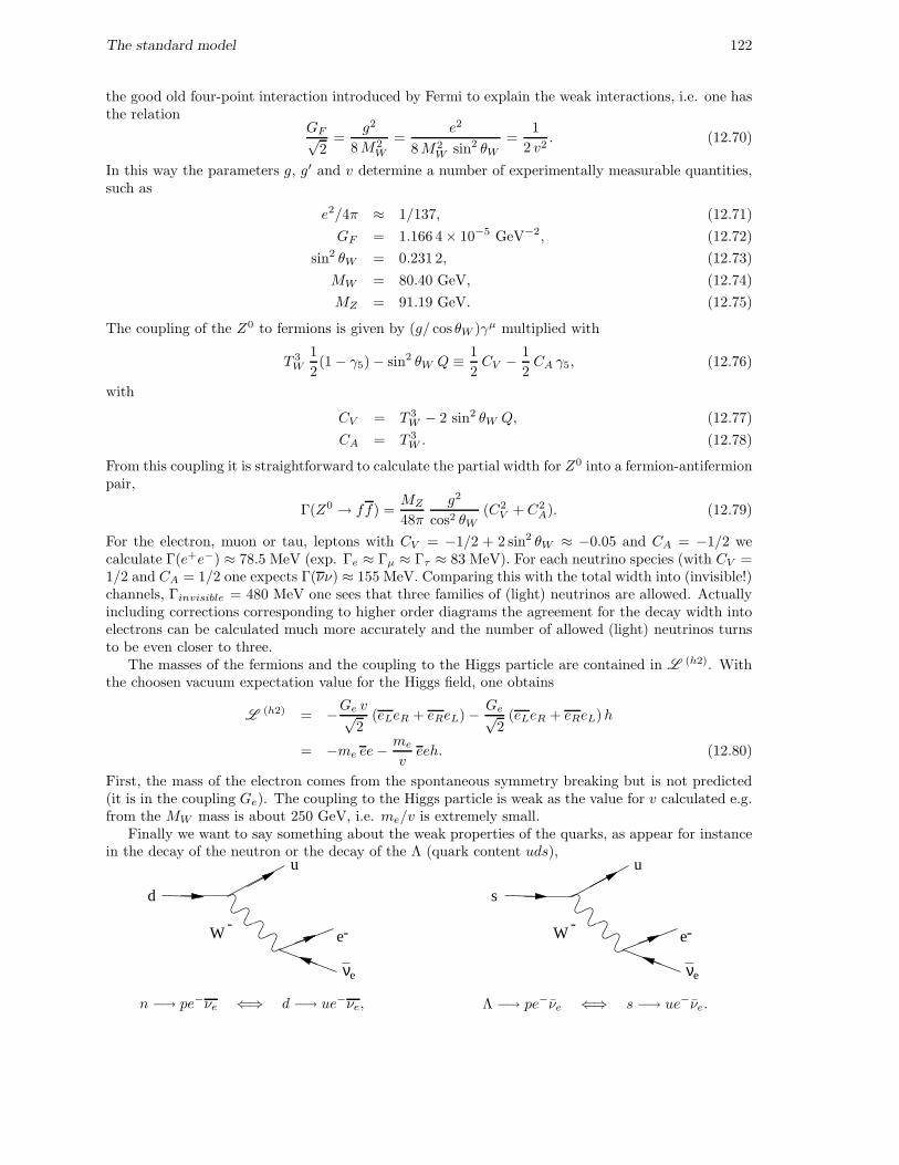
The standard model 122
the good old four-point interaction introduced by Fermi to explain the weak interactions, i.e. one hasthe relation
GF√2
=g2
8M2W
=e2
8M2W sin2 θW
=1
2 v2. (12.70)
In this way the parameters g, g′ and v determine a number of experimentally measurable quantities,such as
e2/4π ≈ 1/137, (12.71)
GF = 1.166 4× 10⁻⁵ GeV−2, (12.72)
sin2 θW = 0.231 2, (12.73)
MW = 80.40 GeV, (12.74)
MZ = 91.19 GeV. (12.75)
The coupling of the Z0 to fermions is given by (g/ cos θW )γµ multiplied with
T 3W
1
2(1 − γ5) − sin2 θW Q ≡ 1
2CV − 1
2CA γ5, (12.76)
with
CV = T 3W − 2 sin2 θW Q, (12.77)
CA = T 3W . (12.78)
From this coupling it is straightforward to calculate the partial width for Z0 into a fermion-antifermionpair,
Γ(Z0 → ff) =MZ
48π
g2
cos2 θW(C2
V + C2A). (12.79)
For the electron, muon or tau, leptons with CV = −1/2 + 2 sin2 θW ≈ −0.05 and CA = −1/2 wecalculate Γ(e+e−) ≈ 78.5 MeV (exp. Γe ≈ Γµ ≈ Γτ ≈ 83 MeV). For each neutrino species (with CV =1/2 and CA = 1/2 one expects Γ(νν) ≈ 155 MeV. Comparing this with the total width into (invisible!)channels, Γinvisible = 480 MeV one sees that three families of (light) neutrinos are allowed. Actuallyincluding corrections corresponding to higher order diagrams the agreement for the decay width intoelectrons can be calculated much more accurately and the number of allowed (light) neutrinos turnsto be even closer to three.
The masses of the fermions and the coupling to the Higgs particle are contained in L (h2). Withthe choosen vacuum expectation value for the Higgs field, one obtains
L(h2) = −Ge v√
2(eLeR + eReL) − Ge√
2(eLeR + eReL)h
= −me ee−me
veeh. (12.80)
First, the mass of the electron comes from the spontaneous symmetry breaking but is not predicted(it is in the coupling Ge). The coupling to the Higgs particle is weak as the value for v calculated e.g.from the MW mass is about 250 GeV, i.e. me/v is extremely small.
Finally we want to say something about the weak properties of the quarks, as appear for instancein the decay of the neutron or the decay of the Λ (quark content uds),
e-
νe
-W
d
u
n −→ pe−νe ⇐⇒ d −→ ue−νe,
e-
νe
-W
u
s
Λ −→ pe−νe ⇐⇒ s −→ ue−νe.
The standard model 123
The quarks also turn out to fit into doublets of SU(2)W for the lefthanded species and into singletsfor the righthanded quarks. A complication arises as it are not the ’mass’ eigenstates that appear inthe weak isospin doublets but linear combinations of them,
ud′
L
cs′
L
tb′
L
,
where
d′
s′
b′
L
=
Vud Vus Vub
Vcd Vcs Vcb
Vtd Vts Vtb
dsb
L
(12.81)
This mixing allows all quarks with T 3W = −1/2 to decay into an up quark, but with different strength.
Comparing neutron decay and Λ decay one can get an estimate of the mixing parameter Vus in thesocalled Cabibbo-Kobayashi-Maskawa mixing matrix. Decay of B-mesons containing b-quarks allowestimate of Vub, etc. In principle one complex phase is allowed in the most general form of the CKMmatrix, which can account for the (observed) CP violation of the weak interactions. This is only trueif the mixing matrix is at least three-dimensional, i.e. CP violation requires three generations. Themagnitudes of the entries in the CKM matrix are nicely represented using the socalled Wolfensteinparametrization
V =
1 − 12 λ
2 λ λ3A(ρ− i η)−λ 1 − 1
2 λ2 λ2A
λ3 A(1 − ρ− i η) −λ2A 1
+ O(λ4)
with λ ≈ 0.227, A ≈ 0.82 and ρ ≈ 0.22 and η ≈ 0.34. The imaginary part i η gives rise to CP violationin decays of K and B-mesons (containing s and b quarks, respectively).
12.5 Family mixing in the Higgs sector and neutrino masses
The quark sector
Allowing for the most general (Dirac) mass generating term in the lagrangian one starts with
L(h2,q) = −QLφΛdDR −DRΛ†dφ
†QL −QLφcΛuUR − URΛ†uφ
c†QL (12.82)
where we include now the three lefthanded quark doublets in QL, the three righthanded quarks withcharge +2/3 in UR and the three righthanded quarks with charges −1/3 inDR, each of these containing
the three families, e.g. UR =
uR cR tR
. The Λu and Λd are complex matrices in the 3×3 family
space. The Higgs field is still limited to one complex doublet. Note that we need the conjugate Higgsfield to get a U(1)Y singlet in the case of the charge +2/3 quarks, for which we need the appropriateweak isospin doublet
φc =
φ0∗
−φ−
=1√2
v + h
0
.
For the (squared) complex matrices we can find positive eigenvalues,
Λu Λ†u = VuG2u V†u , and Λd Λ†d = Vd G
2d V†d , (12.83)
where Vu and Vd are unitary matrices, allowing us to write
Λu = VuGu W†u and Λd = Vd Gd W
†d , (12.84)
with Gu and Gd being real and positive and Wu and Wd being different unitary matrices. Thus onehas
L(h2,q) =⇒ −DLVd MdW
†dDR −DRWd Md V
†d DL − ULVu MuW
†uUR − URWu Mu V
†uUL (12.85)
The standard model 124
with Mu = Guv/√
2 (diagonal matrix containingmu, mc andmt) and Md = Gdv/√
2 (diagonal matrixcontaining md, ms and mb). One then reads off that starting with the family basis as defined via theleft doublets that the mass eigenstates (and states coupling to the Higgs field) involve the righthanded
states UmassR = W †uUR and Dmass
R = W †dDR and the lefthanded states UmassL = V †uUL and Dmass
L =
V †d DL. Working with the mass eigenstates one simply sees that the weak current coupling to the W±
becomes UL γµDL = U
mass
L γµ V †uVd DmassL , i.e. the weak mass eigenstates are
D′L = DweakL = V †u Vd D
massL = VCKMDmass
L , (12.86)
the unitary CKM-matrix introduced above in an ad hoc way.
The lepton sector (massless neutrinos)
For a lepton sector with a lagrangian density of the form
L(h2,ℓ) = −LφΛeER − ERΛ†eφ
†L, (12.87)
in which
L =
NL
EL
is a weak doublet containing the three families of neutrinos (NL) and charged leptons (EL) and ER isa three-family weak singlet, we find massless neutrinos. As before, one can write Λe = Ve GeW
†e and
we findL
(h2,ℓ) =⇒ −Me
(ELVeW
†eER − ERWeV
†e EL
), (12.88)
with Me = Gev/√
2 the diagonal mass matrix with masses me, mµ and mτ . The mass fields EmassR
= W †eER, EmassL = V †e EL. For the (massless) neutrino fields we just can redefine fields into Nmass
L =V †e NL, since the weak current is the only place where they show up. The W -current then becomesEL γ
µNL = Emass
L γµNmassL , i.e. there is no family mixing for massless neutrinos.
The lepton sector (massive Dirac neutrinos)
In principle a massive Dirac neutrino could be accounted for by a lagrangian of the type
L(h2,ℓ) = −LφΛeER − ERΛ†eφ
†L− LφcΛnNR −NRΛ†nφc†L (12.89)
with three righthanded neutrinos added to the previous case, decoupling from all known interactions.Again we continue as before now with matrices Λe = VeGe W
†e and Λn = Vn GnW
†n, and obtain
L(h2,ℓ) =⇒ −ELVe MeW
†eER − ERWe Me V
†e EL −NLVnMnW
†nNR −NRWnMn V
†nNL. (12.90)
We note that there are mass fields EmassR =W †eER, Emass
L = V †e EL, NmassL = V †nNL andNmass
R =W †nNR
and the weak current becomes EL γµNL = Emass
L γµ V †e VnNmassL . Working with the mass eigenstates
for the charged leptons we see that the weak eigenstates for the neutrinos are NweakL = V †e NL with
the relation to the mass eigenstates for the lefthanded neutrinos given by
N ′L = NweakL = V †e VnN
massL = U †PMNSN
massL , (12.91)
with UPMNS = V †n Ve known as the Pontecorvo-Maki-Nakagawa-Sakata mixing matrix.For neutrino’s this matrix is parametrized in terms of three angles θij with cij = cos θij and
sij = sin θij and one angle δ,
UPMNS =
1 0 00 c23 s230 −s23 c23
c13 0 s13 eiδ
0 1 0−s13 eiδ 0 c13
c12 s12 0−s12 c12 0
0 0 1
, (12.92)

The standard model 125
a parametrization that in principle also could have been used for quarks. In this case, it is particularlyuseful because θ12 is essentially determined by solar neutrino oscillations requiring ∆m2
12 ≈ 8 × 10⁻⁵
eV2 (conventionm2 > m1), while θ23 then is determined by atmospheric neutrino oscillations requiring|∆m2
23| ≈ 2.5×10⁻³ eV2. The mixing is intriguingly close to the Harrison-Perkins-Scott tri-bimaximalmixing matrix
UHPS =
1 0 0
0√
1/2 −√
1/2
0√
1/2√
1/2
√
2/3√
1/3 0
−√
1/3√
2/3 00 0 1
=
√
2/3√
1/3 0
−√
1/6√
1/3 −√
1/2
−√
1/6√
1/3√
1/2
.
(12.93)
The lepton sector (massive Majorana fields)
An even simpler option than sterile righthanded Dirac neutrinos, is to add in Eq. 12.88 a Majoranamass term for the (lefthanded) neutrino mass eigenstates,
Lmass,ν = −1
2
(MLN c
LNL +M∗LNLNcL
), (12.94)
although this option is not attractive as it violates the electroweak symmetry. The way to circumventthis is to introduce as in the previous section righthanded neutrinos. with for the righthanded sectora mass term MR,
Lmass,ν = −1
2
(MRNRN
cR +M∗RN
cRNR
). (12.95)
In order to have more than a completely decoupled sector, one must for the neutrinos as well ascharged leptons, couple the right- and lefthanded species through Dirac mass terms coming from thecoupling to the Higgs sector as in the previous section. Thus (disregarding family structure) one hastwo Majorana neutrinos, one being massive. For the charged leptons there cannot exist a Majoranamass term as this would break the U(1) electromagnetic symmetry. For the leptons, the left- andrighthanded species then just form a Dirac fermion.
For the neutrino sector, the massless and massive Majorana neutrinos, coupled by a Dirac massterm, are equivalent to two decoupled Majorana neutrinos (see below). If the Majorana mass MR ≫MD one actually obtains in a natural way one Majorana neutrino with a very small mass. This iscalled the see-saw mechanism (outlined below).
For these light Majorana neutrinos one has, as above, a unitary matrix relating them to the weakeigenstates. Absorption of phases in the states is not possible for Majorana neutrinos, however, hencethe mixing matrix becomes
VPMNS = UPMNSK with K =
eiα1/2 0 0
0 eiα2/2 00 0 1
. (12.96)
containing three (CP-violating) phases (α1, α2 and δ).
The see-saw mechanism
Consider (for one family N = n) the most general Lorentz invariant mass term for two independentMajorana spinors, Υ′1 and Υ′2 (satisfying Υc = Υ and as discussed in chapter 6, Υc
L ≡ (ΥL)c = ΥR
and ΥcR = ΥL). We use here the primes starting with the weak eigenstates. Actually, it is easy to see
that this incorporates the Dirac case by considering the lefthanded part of Υ′1 and the righthandedpart of Υ′2 as a Dirac spinor ψ. Thus
Υ′1 = ncL + nL, Υ′2 = nR + nc
R, ψ = nR + nL. (12.97)
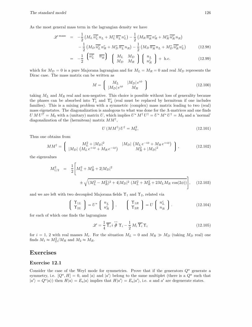
The standard model 126
As the most general mass term in the lagrangian density we have
Lmass = −1
2
(ML nc
L nL +M∗L nL ncL
)− 1
2
(MR nR n
cR +M∗R n
cR nR
)
− 1
2
(MD nc
L ncR +M∗D nL nR
)− 1
2
(MD nR nL +M∗D nc
R ncL
)(12.98)
= −1
2
ncL nR
ML MD
MD MR
nL
ncR
+ h.c. (12.99)
which for MD = 0 is a pure Majorana lagrangian and for ML = MR = 0 and real MD represents theDirac case. The mass matrix can be written as
M =
ML |MD| eiφ
|MD| eiφ MR
(12.100)
taking ML and MR real and non-negative. This choice is possible without loss of generality becausethe phases can be absorbed into Υ′1 and Υ′2 (real must be replaced by hermitean if one includesfamilies). This is a mixing problem with a symmetric (complex) mass matrix leading to two (real)mass eigenstates. The diagonalization is analogous to what was done for the Λ-matrices and one findsU M UT = M0 with a (unitary) matrix U , which implies U∗M † U † = U∗M∗U † = M0 and a ’normal’diagonalization of the (hermitean) matrix MM †,
U (MM †)U † = M20 , (12.101)
Thus one obtains from
MM † =
M2
L + |MD|2 |MD|(ML e
−iφ +MR e+iφ)
|MD|(ML e
+iφ +MR e−iφ)
M2R + |MD|2
, (12.102)
the eigenvalues
M21/2 =
1
2
[
M2L +M2
R + 2|MD|2
±√
(M2L −M2
R)2 + 4|MD|2 (M2L +M2
R + 2MLMR cos(2φ))
]
, (12.103)
and we are left with two decoupled Majorana fields Υ1 and Υ2, related via
Υ1L
Υ2L
= U∗
nL
ncR
,
Υ1R
Υ2R
= U
nc
L
nR
. (12.104)
for each of which one finds the lagrangians
L =1
4Υi i
↔/∂ Υi −
1
2Mi Υi Υi (12.105)
for i = 1, 2 with real masses Mi. For the situation ML = 0 and MR ≫ MD (taking MD real) onefinds M1 ≈M2
D/MR and M2 ≈MR.
Exercises
Exercise 12.1
Consider the case of the Weyl mode for symmetries. Prove that if the generators Qa generate asymmetry, i.e. [Qa, H ] = 0, and |a〉 and |a′〉 belong to the same multiplet (there is a Qa such that|a′〉 = Qa|a〉) then H |a〉 = Ea|a〉 implies that H |a′〉 = Ea|a′〉, i.e. a and a′ are degenerate states.
The standard model 127
Exercise 12.2
Derive for the vector and axial vector currents, ~V µ = ψγµ ~Tψ and ~Aµ = ψγµγ5~Tψ
∂µ~V µ = i ψ [M, ~T ]ψ,
∂µ~Aµ = i ψ M, ~T γ5 ψ.
Exercise 12.3
(a) The coupling of the Z0 particle to fermions is described by the vertex
−i g
2 cos θW
(
CfV γ
µ − CfA γ
µγ5
)
,
with
CV = T 3W − 2Q sin2 θW ,
CA = T 3W .
Write down the matrix element squared (averaged over initial spins and summed over finalspins) for the decay of the Z0. Neglect the masses of fermions and use the fact that the sumover polarizations is
3∑
λ=1
ǫ(λ)µ (p)ǫ(λ)∗
ν (p) = −gµν +pµpν
M2.
to calculate the width Γ(Z0 → f f),
Γ(Z0 → f f) =MZ
48π
g2
cos2 θW
(
Cf 2V + Cf 2
A
)
.
(b) Calculate the width to electron-positron pair, Γ(Z0 → e+e−), and the width to a pair of neu-trino’s, Γ(Z0 → νeνe). The mass of the Z0 is MZ = 91 GeV, the weak mixing angle is given bysin2 θW = 0.231.
Exercise 12.4
Calculate the lifetime τ = 1/Γ for the top quark (t) assuming that the dominant decay mode is
t → b +W+.
In the standard model this coupling is described by the vertex
−i g2√
2(γµ − γµγ5) .
The masses are mt ≈ 175 GeV, mb ≈ 5 GeV and MW ≈ 80 GeV.
Exercise 12.5
Show that the coupling to the Higgs (W+W−h, ZZh, hhh and e+e−h) are proportional to the masssquared (bosons) or mass (fermions) of the particles. Note that you can find the answer withoutexplicit construction of the interaction terms in the lagrangian.
Exercise 12.6
Check that the use of the Wolfenstein parametrization in the CKM matrix indeed gives a unitarymatrix, at least up to a high (which?) order in λ.

The standard model 128
Exercise 12.7
In this exercise two limits are investigated for the two-Majorana case.
(a) Calculate for the special choice ML = MR = 0 and MD real, the mass eigenvalues and showthat the mixing matrix is
U =1√2
1 1i −i
which enables one to rewrite the Dirac field in terms of Majorana spinors. Give the explicitexpressions that relate ψ and ψc with Υ1 and Υ2.
(b) A more interesting situation is 0 = ML < |MD| ≪ MR, which leads to the socalled see-sawmechanism. Calculate the eigenvalues ML = 0 and MR = MX . Given that neutrino massesare of the order of 0.05 eV, what is the mass MX if we take for MD the electroweak symmetrybreaking scale v (about 250 GeV).


