(Continuous Variables) Quantum Optics, Quantum Information ...
QUANTUM ENGINEERING WITH QUANTUM OPTICS
A DISSERTATION
SUBMITTED TO THE DEPARTMENT OF APPLIED PHYSICS
AND THE COMMITTEE ON GRADUATE STUDIES
OF STANFORD UNIVERSITY
IN PARTIAL FULFILLMENT OF THE REQUIREMENTS
FOR THE DEGREE OF
DOCTOR OF PHILOSOPHY
Joseph Kerckhoff
May 2011

iv

Abstract
Despite initial set backs in the 1980s, the prospect for large scale integration of optical
devices with high spatial-density and low energy consumption for information appli-
cations has grown steadily in the past decade. At the same time these advances have
been made towards classical information processing with integrated optics, largely
in an engineering context, a broad physics community has been pursuing quantum
information processing platforms, with a heavy emphasis on optics-based networks.
But despite these similarities, the two communities have exchanged models and tech-
niques to a very limited degree. The aim of this thesis is to provide examples of
the advantages of an engineering perspective to quantum information systems and
quantum models to systems of interest in optical engineering, in both theory and
experiment.
I present various observations of ultra-low energy optical switching in a cavity
quantum electrodynamical (cQED) system containing a single emitter. Although
such devices are of interest to the engineering community, the dominant, classical op-
tical models used in the field are incompatible with several photon, ultra-low energy
devices like these that evince a discrete Hilbert space and are perturbed by quantum
fluctuations. And in complement to this, I also propose a nanophotonic/cQED ap-
proach to building a self-correcting quantum memory, simply “powered” by cw laser
beams and motivated by the conviction that for quantum engineering to be a viable
paradigm, quantum devices will have to control themselves. Intuitive in its operation,
this network represents a coherent feedback network in which error correction occurs
entirely “on-chip,” without measurement, and is modeled using a flexible formalism
that suggests a quantum generalization of electrical circuit theory.
v

Acknowledgement
One can’t get through graduate school without help from a ridiculously large number
of people (and a few cats). Here I’ll try to acknowledge a few.
Tiku Majumder, my undergraduate advisor, who paid me to do research after
only a single class of undergraduate physics and with whom I continued to work for
much of my “free time” in college. His (continuing) encouragement and advice has so
much to do with so many of my career choices in college and beyond. He’s seriously
great; look at where all his students have gone.
Ben Lev, into whose research shoes I stepped immediately after joining Hideo’s
group at Caltech. In three short months, on top of everything else he had going on,
he was savvy enough to impart enough knowledge and excitement for the work to
give me an excellent start.
Paul Barclay, my first collaborator, friend and housemate. Through him I had the
privilege early on of seeing how a physicist learns new things and he always worked
with me as an equal, even with all his experience. Through him, I’ve also met so
many other great scientists at Caltech and HP.
Luc Bouten, with whom I actively worked only briefly and remotely, but whose
mark has been indelible. If he hadn’t been so bored with making figures, I never
would have learned about QSDEs. I wouldn’t be a “half-theorist” if it wasn’t for his
help, encouragement and writings.
Rick Pam, my teaching teacher, through whom I learned so much about inspiring
younger students and conducting great courses. Every applied physics grad student
should be his TA. I’m greatly in Mark Kasevich and Doug Osheroff’s debt in this
regard too.
vi
Dmitri Pavlichin, enduring co-author. I don’t understand why we work well to-
gether, but we do. He’s taught me a lot and I’ve taught myself a lot trying to teach
him.
Tony Miller, I don’t know 1/5th of the technical things he knows. His practical,
technical and actual gifts have been an essential part of me actually getting things
done around here.
Hendra Nurdin was so critical in moving a solid third of this thesis work from
mere concept to actual practice. His help, advice and interests have opened a whole
new field to me.
Mike Armen, it’s hard to know where to start. I snatched so many things and
thoughts he knowingly and unknowingly prepared, sometimes for me and sometimes
not. Seriously, he’s the best style coach I’ve had. (in physics)
The Group. No, I’m not going to list them all. Everyone hates that anyways.
Science is a social enterprise and and I can’t imagine having done any of this without
being in and around such talented people.
Hideo Mabuchi was perhaps the perfect advisor for me. The support, advice,
encouragement, freedom, talent and resources he’s given me have been rare indeed.
Perhaps my highest praise is that I can’t think of a better place for me to have spent
the past six years than in the group he’s constructed.
Oz and GC. I don’t care what everyone else says. You’re great. May your little
lives be full of packing tissue and turkey.
Mom and Dad, emotional, administrative, culinary, financial, and life support.
Everyone’s jealous that they’ve let me live with them the past two years (seriously,
they are). It would be an understatement to say I owe everything to them.
Sara, would you believe it if I told you I did this all for you? Let’s get married!
vii

Contents
Abstract v
Acknowledgement vi
I Quantum Optics with Quantum Stochastic Differential
Equations 3
1 Quantum stochastic differential equations 6
1.1 The quantum noise process . . . . . . . . . . . . . . . . . . . . . . . . 7
1.2 Quantum stochastic calculus . . . . . . . . . . . . . . . . . . . . . . . 9
1.3 The master equation . . . . . . . . . . . . . . . . . . . . . . . . . . . 15
1.4 The series product . . . . . . . . . . . . . . . . . . . . . . . . . . . . 16
1.5 Multiple fields . . . . . . . . . . . . . . . . . . . . . . . . . . . . . . . 19
1.6 Adiabatic elimination with QSDEs . . . . . . . . . . . . . . . . . . . 20
2 Optical measurements and state estimation 22
2.1 Optical measurement . . . . . . . . . . . . . . . . . . . . . . . . . . . 22
2.1.1 Photon counting . . . . . . . . . . . . . . . . . . . . . . . . . 22
2.1.2 Homodyne measurement . . . . . . . . . . . . . . . . . . . . . 24
2.1.3 Calculating photocurrent statistics . . . . . . . . . . . . . . . 26
2.2 Quantum trajectories . . . . . . . . . . . . . . . . . . . . . . . . . . . 31
2.2.1 The stochastic Schrodinger equation . . . . . . . . . . . . . . 32
viii

II Quantum ‘Bistability’ in Cavity QED 35
3 The cQED model 37
3.1 The cQED master equation . . . . . . . . . . . . . . . . . . . . . . . 37
3.2 The QSDE representation . . . . . . . . . . . . . . . . . . . . . . . . 41
3.3 The Maxwell-Bloch equations . . . . . . . . . . . . . . . . . . . . . . 43
4 Single atom ‘bistability’ 47
4.1 Absorptive ‘bistability’ . . . . . . . . . . . . . . . . . . . . . . . . . . 48
4.2 Dispersive ‘bistability’ . . . . . . . . . . . . . . . . . . . . . . . . . . 55
4.2.1 The Jaynes-Cumming ladder . . . . . . . . . . . . . . . . . . . 55
4.2.2 Phase ‘bistability’ in highly-excitated cQED . . . . . . . . . . 58
4.3 Toward optical control . . . . . . . . . . . . . . . . . . . . . . . . . . 61
4.3.1 Driven transition dynamics . . . . . . . . . . . . . . . . . . . . 62
4.3.2 Dynamics without control . . . . . . . . . . . . . . . . . . . . 64
4.3.3 Control dynamics . . . . . . . . . . . . . . . . . . . . . . . . . 66
4.3.4 Simulation of a controlled quantum dot system . . . . . . . . 67
5 The broadband cavity QED apparatus 70
5.1 The atom . . . . . . . . . . . . . . . . . . . . . . . . . . . . . . . . . 71
5.2 The cavity . . . . . . . . . . . . . . . . . . . . . . . . . . . . . . . . . 72
5.3 A tour of the apparatus . . . . . . . . . . . . . . . . . . . . . . . . . 76
5.3.1 Science cavity locking and probing . . . . . . . . . . . . . . . 76
5.3.2 Delivering the atoms . . . . . . . . . . . . . . . . . . . . . . . 80
5.3.3 Transit detection and homodyne measurements . . . . . . . . 81
6 Observations of optical ‘bistability’ 84
6.1 Amplitude ‘bistability’ . . . . . . . . . . . . . . . . . . . . . . . . . . 84
6.2 Phase ‘bistability’ . . . . . . . . . . . . . . . . . . . . . . . . . . . . . 90
ix

III Autonomous Nanophotonic Quantum Memories 98
7 Preliminary Models 102
7.1 Quantum error correction . . . . . . . . . . . . . . . . . . . . . . . . 102
7.1.1 The bit-flip and phase-flip codes . . . . . . . . . . . . . . . . . 103
7.1.2 The 9 qubit Bacon-Shor code . . . . . . . . . . . . . . . . . . 106
7.2 cQED parity networks . . . . . . . . . . . . . . . . . . . . . . . . . . 109
7.2.1 Physical model of a cQED TLS . . . . . . . . . . . . . . . . . 109
7.2.2 Continuous parity measurement in a nanophotonic network . . 115
8 Autonomous QEC nanophotonic networks 122
8.1 An autonomous bit-/phase-flip network . . . . . . . . . . . . . . . . . 123
8.1.1 Intuitive operation . . . . . . . . . . . . . . . . . . . . . . . . 123
8.1.2 Network model and dynamics . . . . . . . . . . . . . . . . . . 128
8.2 The autonomous subsystem QEC network . . . . . . . . . . . . . . . 132
Bibliography 141
x

List of Tables
1.1 The quantum Ito table . . . . . . . . . . . . . . . . . . . . . . . . . . 12
7.1 Bit-flip code syndrome measurements . . . . . . . . . . . . . . . . . . 104
xi

List of Figures
1.1 QSDE as I/O model . . . . . . . . . . . . . . . . . . . . . . . . . . . 10
1.2 QSDE network example . . . . . . . . . . . . . . . . . . . . . . . . . 17
2.1 Optical homodyne measurement . . . . . . . . . . . . . . . . . . . . . 24
3.1 cQED concept . . . . . . . . . . . . . . . . . . . . . . . . . . . . . . . 38
4.1 Steady state absorptive bistability . . . . . . . . . . . . . . . . . . . . 49
4.2 Steady state MBE vs. quantum solutions . . . . . . . . . . . . . . . . 50
4.3 Amplitude bistability W-functions . . . . . . . . . . . . . . . . . . . . 51
4.4 Amplitude bistability trajectories . . . . . . . . . . . . . . . . . . . . 52
4.5 Steady state amplitude bistability photocurrents . . . . . . . . . . . . 53
4.6 The Jaynes-Cummings spectrum . . . . . . . . . . . . . . . . . . . . 56
4.7 cQED transmission spectrum . . . . . . . . . . . . . . . . . . . . . . 57
4.8 Phase bistability steady state W-functions . . . . . . . . . . . . . . . 60
4.9 Controlled phase switching in a quantum dot . . . . . . . . . . . . . . 68
5.1 Cavity mounting schematic . . . . . . . . . . . . . . . . . . . . . . . . 72
5.2 Cavity transmission noise . . . . . . . . . . . . . . . . . . . . . . . . 75
5.3 Cavity mount mechanical resonances . . . . . . . . . . . . . . . . . . 76
5.4 Cavity stabilization and probing optics . . . . . . . . . . . . . . . . . 77
5.5 Laser frequency noise spectrum . . . . . . . . . . . . . . . . . . . . . 79
5.6 Atom transits with weak heterodyne detection . . . . . . . . . . . . . 82
6.1 Experiment concept . . . . . . . . . . . . . . . . . . . . . . . . . . . . 85
xii
6.2 Experimental absorptive ‘bistability’ signal . . . . . . . . . . . . . . . 86
6.3 Experimental steady state absorptive ‘bistability’ . . . . . . . . . . . 87
6.4 Photocurrent autocorrelation . . . . . . . . . . . . . . . . . . . . . . 88
6.5 cQED absorptive hysteresis. . . . . . . . . . . . . . . . . . . . . . . . 89
6.6 Near-detuned phase ‘bistabiliy’ . . . . . . . . . . . . . . . . . . . . . 91
6.7 Experimental phase ‘bistability’ signal . . . . . . . . . . . . . . . . . 92
6.8 Phase switching rate estimation . . . . . . . . . . . . . . . . . . . . . 93
6.9 High-drive-induced atom loss . . . . . . . . . . . . . . . . . . . . . . 94
6.10 Enhanced switching rate with cw control probe . . . . . . . . . . . . 97
6.11 A traditional quantum ‘circuit’ . . . . . . . . . . . . . . . . . . . . . 100
7.1 9 qubit subsystem code operator groups . . . . . . . . . . . . . . . . 106
7.2 One-sided cavity reflection . . . . . . . . . . . . . . . . . . . . . . . . 110
7.3 cQED qubit level structure . . . . . . . . . . . . . . . . . . . . . . . . 111
7.4 Cavity parity probe network . . . . . . . . . . . . . . . . . . . . . . . 116
7.5 Bell-state production in a cQED network . . . . . . . . . . . . . . . . 117
7.6 Performance of reduced model as an approximate quantum filter . . . 121
8.1 The autonomous bit-/phase-flip nanophotonic network . . . . . . . . 124
8.2 cQED relay level structure . . . . . . . . . . . . . . . . . . . . . . . . 125
8.3 QSDE circuit schematic for the bit-/phase-flip network . . . . . . . . 127
8.4 Logical fidelity in bit-flip network . . . . . . . . . . . . . . . . . . . . 131
8.5 The autonomous 9-qubit nanophotonic network . . . . . . . . . . . . 133
8.6 Alternate 9-qubit probe routing . . . . . . . . . . . . . . . . . . . . . 135
8.7 Logical fidelity in the 9-qubit network . . . . . . . . . . . . . . . . . . 138
8.8 Correction of different error classes in 9-qubit network . . . . . . . . . 139
xiii

xiv

Outline
On some days, my research has been motivated by the expectation that quantum
optics will be a future discipline of electrical engineering. On others, it’s been driven
by a notion that a generalized concept of the electrical circuit should guide a future
strain of quantum optics. Whichever way, both the experiments and theoretical work
described below have rested heavily on a unifying formalism of open quantum optical
systems that makes both perspectives natural, at the level of individual devices and
for large scale networks.
Part I introduces this formalism. While quantum stochastic differential equations
(QSDEs) have been developed by many authors over the past three decades, I have
increasingly recognized a need for an informal introduction to the formalism to com-
pliment the technical literature. Chapter 1 describes this approach to modeling open
quantum optical systems as noisy, Markovian dynamical processes. The interpreta-
tion of the QSDE model as describing input-output (I/O) devices for quantum fields
is emphasized, as well as a method for constructing composite network models built
from series and parallel interconnections of individual devices. Chapter 2 describes
how continuous optical measurement is naturally incorporated into the formalism and
gives it much of its utility, bringing together theories of weak measurement and real
time state estimation.
Part II centers on various observations of spontaneous optical switching of the field
transmitted by a Fabry-Perot cavity containing a single, strongly coupled Cs atom.
While confirming long-standing theoretical predictions, these observations also high-
light that binary optical signaling persists even into the ‘deep quantum’ regime of
1

2
devices with countable photon numbers and single emitters. As nanophotonic re-
search pushes into the attojoule device regime, these observations underscore that
quantum optical models will soon be essential for understanding nonlinear optical
device physics, offering both technological problems and opportunities not captured
by commonly employed semiclassical models. Chapter 3 introduces models for single-
atom cavity quantum electrodynamics (cQED) in both a semiclassical approximation
and as a QSDE optical I/O device. Chapter 4 describes how both models predict
an I/O bistable response as the cQED device is driven at and into the atomic sat-
uration regime. The picture that emerges is subtle, however: the quantum optical
model (the more accurate model) both predicts disrupted signal stability (due to
fractionally large quantum fluctuations) and sometimes enhanced signal discretiza-
tion (due to a discrete Hilbert space). Two different I/O regimes are considered,
absorptive/amplitude bistability, which occurs at the cusp of atomic saturation, and
dispersive/phase bistability which appears well into the saturation regime. Chap-
ter 5 then introduces the experimental apparatus built to measure the optical field
transmitted by a high finesse Fabry-Perot cavity containing a single, strongly coupled
Cs atom with broadband optical homodyne detection, emphasizing the improvements
and continuing issues in the system since 2009. Finally, chapter 6 reports observations
of the predictions introduced in chapter 4.
Part III considers how nanophotonic network models could aid the development
of quantum memories. This work imports abstract concepts of quantum error correc-
tion (QEC) into a hardware-specific circuit formalism, yielding an approach to QEC
that is well-suited to developing robust quantum technologies. These technologically
homogenous nanophotonic networks are noteworthy in that the error suppression oc-
curs continuously and autonomously, that is with a minimal amount of oversight
and supporting hardware. Chapter 7 first introduces the specific QEC codes our
designs emulate. It also details a physical model for cQED devices and networks ap-
propriate to implement these codes and characterizes how their performance rapidly
improves in a nanophotonic context. Finally, chapter 8 describes two types of designs
for nanophotonic networks that emulate three different codes and characterizes their
performance.

Part I
Quantum Optics with Quantum
Stochastic Differential Equations
3

Introduction
This first part introduces a formalism for modeling open quantum optical systems
that has been essential in both my experimental and theoretical work. While quan-
tum stochastic differential equations (QSDEs) represent a rigorous stochastic dyami-
cal modeling unfamiliar to most physicists, the approach becomes physically intuitive
once internalized. QSDEs take quantum field theory as the underlying physical model
[GPZ92, GZ04], but their manipulations appear as a quantum generalization of elec-
trical circuit theory and are able to adapt many powerful techniques from classical
control theory into the quantum regime, e.g. [NJD09, NJP09, JNP08, GJ09b]. Suf-
ficiently general to describe the dynamics of most systems foreseeable in quantum
optical systems, with or without measurement of optical fields, with or without stabi-
lizing (coherent optical or classical ‘electrical’) feedback, these models are attractive
due to their physically intuitive formulation [KNPM10] that admits both analytic
and numerical analysis through connections to theories of continuous measurement
[Bar90], state estimation [BvHJ07] and control [NJP09].
While the theory of QSDEs and QSDE networks has been developed by many
authors in the past three decades, the literature is fairly mathematical [HP84, Par92,
Fag90, GPZ92, Bar90, BvHJ07, BvHS08, GJ09b]. Over the past few years, many
students have asked me to explain how to use QSDEs in their own work, but I’ve
found that they usually get discouraged by the formal derivations and manipulations.
Somehow, I got through that initial hurdle and they have been essential in my work
ever since. As I feel there is a bright future for this formalism and that it has a
natural role to play in the emerging field of quantum optical engineering, this first
part introduces QSDEs and their manipulations that underlie most of the analysis
4

5
in the subsequent experimental and theoretical chapters. As the formalism has been
incredibly useful to me as a tool, not an object of study in itself, the concepts are
presented in a non-formal manner, at a level appropriate for a reader with grounding
in more mainstream quantum optics. The ‘results’ in this part are pedagogical, if
that, aiming to present an intuitive explanation of QSDEs to complement the proper
formulation found in the literature.

Chapter 1
Quantum stochastic differential
equations
Loosely, quantum stochastic differential equation (QSDEs) are a method of modeling
open quantum optical systems that resembles a quantum version of electrical circuit
theory. Free, bosonic quantum fields play the role of electrical current-carrying wires,
while localized systems like atoms or optical resonators function as input-output (I/O)
devices that affect the fields, but are also affected by them.
QSDEs are a rigorous, self-consistent mathematical formalism, but they are useful
because they represent a good approximation of most systems foreseeable in quantum
optics [GZ04, GPZ92]. This chapter begins by motivating the reasonableness of using
this representation to describe physical quantum optic phenomena, but will gradually
drift into working just with the abstracted objects themselves.
This introduction is quick and is meant to give the reader a glimpse of all the
steps on the way to a complete theory of QSDEs and their physical justification. A
more complete picture (although much longer) may be constructed through references
cited along the way, especially [GZ04, GPZ92, BvHJ07, Bar90, GJ09b, BvHS08].
6

1.1. THE QUANTUM NOISE PROCESS 7
1.1 The quantum noise process
As is common when considering an open quantum system, the global system composed
of a system (i.e. a localized system like an atom or optical resonator) and bath (i.e.
free optical fields) is considered ‘closed’ and its dynamics may be described with the
Hamiltonian
H0 Hs Hb Hi (1.1)
where the system and bath have their own, internal evolution govern by Hs and Hb,
respectively, and the two subsystems are also coupled via the interaction Hi. Hereon,
I will use “system” to refer to the localized system (with Hamiltonian Hs) and “global
system” to refer to the totality composed of isolated system(s) and bath(s). In the
quantum optics context, we assume that the bath is comprised of a dense spectrum
of bosonic fields, such that (~ 1)
Hb » 80
dωωb:pωqbpωq (1.2)
where bpωq are annihilation operator “densities,” : the Hermitian conjugate, andrbpωq, b:pω1qs δpω ω1q. We don’t need to specify anything about Hs yet, but the
coupling between the system and bath has to have a particular linear form
Hi i
» 80
dωaκpωqpcb:pωq c:bpωqq (1.3)
where c is some operator on the system and κpωq is a real-valued function describing
the strength of the interaction. Already, this interaction typically makes an approxi-
mation, commonly known as the rotating wave approximation, that coupling terms of
the form c:b:pωq and its hermitian conjugate (which exist in a complete description)
oscillate too quickly to influence the relatively slow dynamics we care about [GPZ92].
This approximation is itself only good when Hi is assumed to be weak compared to
the evolution of both c under Hs and bpωq under Hb. This is usually a very good ap-
proximation in quantum optics, as the coupling rates typically operate on GHz-MHz
frequency scales (call these κ frequency scales), while the principle system and bath

8 CHAPTER 1. QUANTUM STOCHASTIC DIFFERENTIAL EQUATIONS
operators oscillate at frequencies of order 100s of THzs (i.e. optical frequencies).
It is convenient to go into an interaction frame such that the global system states
become |ψ1ty Ñ eipHsHbqt|ψ1ty |ψty (1.4)
and the operators also gain some time-dependence, accordingly. In this picture, the
global state evolves according to the Schrodinger equation
d
dt|ψty » 8
0
dω?κpωqpcptqb:pω, tq c:ptqbpω, tqq|ψty. (1.5)
Given Hb, we have bpω, tq eiωtbpω, 0q, and it is typical that in this picture cptq eiω0tc, where ω0 is in the optical regime. In this case we can rewrite equation (1.5)
asd
dt|ψty a2πκpω0qpcb:ptq c:bptqq|ψty, (1.6)
where
bptq 1a2πκpω0q » 8
0
dωaκpωqbpω, 0qeipωω0qt. (1.7)
At this point, we make a Markov approximation that the coupling strength κpωqvaries slowly around ω0, slow compared to the inverse time scales κ on which we expect
the interesting dynamics to occur. Also, we allow ourselves to extend the lower limit
on the definition of bptq to 8, justifiable as ω0 " κ. With these approximations in
hand, we can calculate the commutator of bptq [GPZ92]rbptq, b:pt1qs » 88 dωeipωω0qptt1q κpωq2πκpω0q δpt t1q. (1.8)
Thus, due to our approximations, bptq looks very much like a delta-correlated white
noise process. In fact, with our aim set on a QSDE formalism, it is better to think of
it as a sort of quantum noise process, rather than as its definition (1.7) as the integral
of Schrodinger-picture operator densities in an interaction frame. Each bptq exerts itsinfluence on the global system in Eq. (1.6) in chronological succession, independent
of all other bpt1q [GPZ92]. For this reason, bptq may be considered noise ‘inputs’ to
the system [GZ04], with the ‘time’ t indexing the time at which the operator bptq

1.2. QUANTUM STOCHASTIC CALCULUS 9
interacts with the system; call them binptq bptq. Essentially a Fourier transform
of bpωq, bptq may also be thought of as a time-domain annihilation operator density,
acting on the infinitesimal segment of field that interacts with the system at time t.
Now, for t1 ¡ t, consider
boutptq 1?2π
» 88 dωeipωω0qptt1qbpω, t1q, (1.9)
which is almost the same as binptq, except that it is defined in terms of bpω, t1q in the
‘future.’ Comparing binptq and boutptq is more naturally done in the Heisenberg picture.
In this picture, given our interaction Hamiltonian, it may be straightforwardly shown
that for any choice of t1 in the definition of boutptq [GZ04]
boutptq binptq a2πκpω0qcptq. (1.10)
In other words, boutptq is a linear superposition of the ‘noise’ that interacts with the
system at time t, plus a contribution from the system at time t, proportional to cptq(which is itself dependent on all previous input values of binpt1q, t1 t). For this
reason, boutptq may be considered the field ‘output’ of the system at time t.
1.2 Quantum stochastic calculus
Although it may appear we now have a very nice quantum optic I/O theory, our input
and output operators are highly singular. For example, we immediately run into a
problem if we try to calculate the expectation of bptqb:ptq on the vacuum field state
[GPZ92] xvac|bptqb:ptq|vacy xvac|bptqb:ptq b:ptqbptq|vacy δp0q (1.11)
where we have used bptq|vacy 0. Fortunately, a solution to problems of this nature
is well known for classical noisy systems. Roughly speaking, we consider bptq to be the

10 CHAPTER 1. QUANTUM STOCHASTIC DIFFERENTIAL EQUATIONS
L L
dB T
dj (B )τ τ
Hs
tT>t τ<t
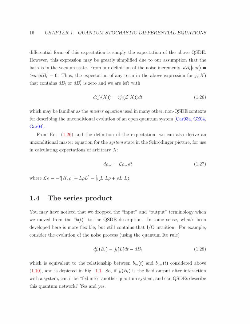
Figure 1.1: A cartoon depiction of the QSDE I/O formulation. A single, free opticalmode couples via an operator L to a fixed Hamiltonian system (Hs), affecting itand being affected by it. After interaction, the field continues to propagate, and ispossibly detected. The fundamental noise increment dBt may be thought of as theannihilation operator on an infinitesimal segment of the field that interacts with thesystem at time t. At time t, the segment indexed by T ¡ t has yet to interact withthe system (an ‘input’), but the segment indexed by τ t already has (and is an‘output’), transforming its noise increment as djτ pBτ q (Eq. (1.28)).(ill-defined) derivative of some rapidly varying, noise integral [GPZ92, GZ04, Gar04]
Bt Bt0 » tt0
dt1bpt1q » tt0
dBt1 ,B:t B
:t0
» tt0
dt1b:pt1q » tt0
dB:t1. (1.12)
In a classical analogy, bptq is like the velocity of a particle undergoing Brownian
motion (i.e. diffusion), whereas Bt is its position. The usual terminology is to call
Bt the annihilation and B:t the creation process. Later on we’ll also use another noise
process, called the gauge process [Bar90]
Λt Λt0 » tt0
dt1b:pt1qbpt1q » tt0
dΛt1. (1.13)
Note that through these definition and the commutator of bptq, Bt, B:t and Λt act as
the identity on processes that don’t overlap with the time interval p0, ts, a property
called adapted [BvHJ07, Bar90]. With these definitions, our Schrodinger equation
1.2. QUANTUM STOCHASTIC CALCULUS 11
above (1.6) is more accurately considered an integral equation|ψ, ty |ψ, t0y » tt0
pLdB:t1 L:dBt1q|ψ, t1y, (1.14)
where we have now defined the coupling operator L a2πκpω0qc. Replacing the
bptq and b:ptq with dBt and dB:t in (1.6) produces a quantum stochastic differential
equation (QSDE) representing the evolution of the global system in the Schrodinger
picture,
d|ψty pLdB:t L:dBtq|ψty, (1.15)
but it is understood as merely a symbolic abbreviation of integral equation (1.14).
This brings us to the critical question of how do we calculate these integrals? It
can be shown that if we require the noises to obey ordinary calculus (e.g. that
dpB:tBtq dpB:
t qBt B:tdpBtq), as would be expected of a physical system described
with “natural” processes and we’ve implicitly assumed so far, then these integrals
have to be understood as the limit (for example)» tt0
fpt1qdBt1 limnÑ8 1
2
n
i0
pfpiq fpi 1qqpBi1 Biq (1.16)
where fptq is some adapted function, and is known as a Stratonovich integral [GPZ92,
GZ04, Gar04]. However, there is a problem here: fpi1q does not commute with the
interval Bpi 1q Bpiq in general, which makes working with these equations very
awkward. This means that » tt0
fpt1qdBt1 » tt0
dBt1fpt1q, (1.17)
causing a practical nightmare in any integral calculation (in a classical analogy, the
noise processes fptq and dBt are correlated and their product is difficult to integrate).
An alternative definition of the stochastic integral is» tt0
fpt1qdBt limnÑ8 n
i0
fpiqpBi1 Biq (1.18)
12 CHAPTER 1. QUANTUM STOCHASTIC DIFFERENTIAL EQUATIONS
dXdY dBkt dB
k:t dΛklt dt
dBit 0 δikdt δikdB
lt 0
dBi:t 0 0 0 0
dΛijt 0 δjkdBi:t δjkdΛ
ilt 0
dt 0 0 0 0
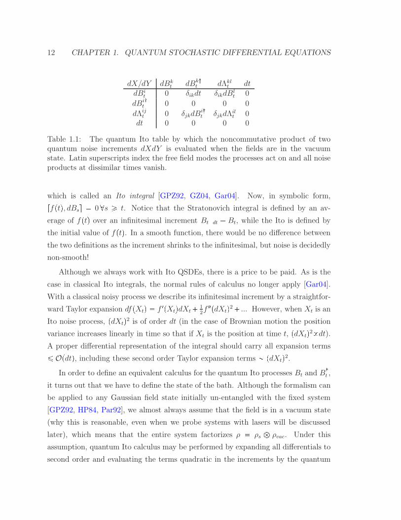
Table 1.1: The quantum Ito table by which the noncommutative product of twoquantum noise increments dXdY is evaluated when the fields are in the vacuumstate. Latin superscripts index the free field modes the processes act on and all noiseproducts at dissimilar times vanish.
which is called an Ito integral [GPZ92, GZ04, Gar04]. Now, in symbolic form,rfptq, dBss 0 s ¥ t. Notice that the Stratonovich integral is defined by an av-
erage of fptq over an infinitesimal increment Btdt Bt, while the Ito is defined by
the initial value of fptq. In a smooth function, there would be no difference between
the two definitions as the increment shrinks to the infinitesimal, but noise is decidedly
non-smooth!
Although we always work with Ito QSDEs, there is a price to be paid. As is the
case in classical Ito integrals, the normal rules of calculus no longer apply [Gar04].
With a classical noisy process we describe its infinitesimal increment by a straightfor-
ward Taylor expansion dfpXtq f 1pXtqdXt 12f 2pdXtq2 ... However, when Xt is an
Ito noise process, pdXtq2 is of order dt (in the case of Brownian motion the position
variance increases linearly in time so that if Xt is the position at time t, pdXtq29dt).A proper differential representation of the integral should carry all expansion terms¤ Opdtq, including these second order Taylor expansion terms pdXtq2.
In order to define an equivalent calculus for the quantum Ito processes Bt and B:t ,
it turns out that we have to define the state of the bath. Although the formalism can
be applied to any Gaussian field state initially un-entangled with the fixed system
[GPZ92, HP84, Par92], we almost always assume that the field is in a vacuum state
(why this is reasonable, even when we probe systems with lasers will be discussed
later), which means that the entire system factorizes ρ ρs b ρvac. Under this
assumption, quantum Ito calculus may be performed by expanding all differentials to
second order and evaluating the terms quadratic in the increments by the quantum
1.2. QUANTUM STOCHASTIC CALCULUS 13
Ito table 1.1. For example, for the adapted quantum stochastic processes X and Y ,
we calculate
dpXY q pdXqY XpdY q dXdY, (1.19)
where the last term is evaluated according to the above table. Taken together, the
rule of differentiation and the table above are called the quantum Ito rule [HP84,
GPZ92, BvHJ07].
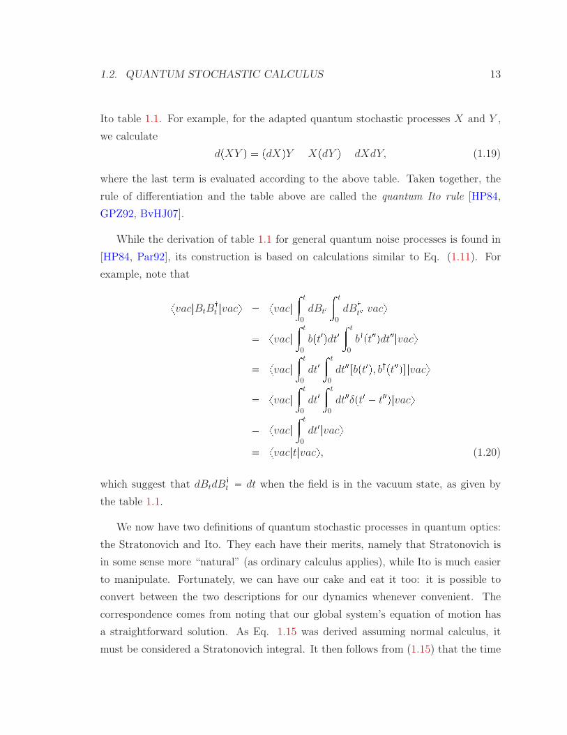
While the derivation of table 1.1 for general quantum noise processes is found in
[HP84, Par92], its construction is based on calculations similar to Eq. (1.11). For
example, note thatxvac|BtB:t |vacy xvac| » t
0
dBt1 » t0
dB:t2 |vacy xvac| » t
0
bpt1qdt1 » t0
b:pt2qdt2|vacy xvac| » t0
dt1 » t0
dt2rbpt1q, b:pt2qs|vacy xvac| » t0
dt1 » t0
dt2δpt1 t2q|vacy xvac| » t0
dt1|vacy xvac|t|vacy, (1.20)
which suggest that dBtdB:t dt when the field is in the vacuum state, as given by
the table 1.1.
We now have two definitions of quantum stochastic processes in quantum optics:
the Stratonovich and Ito. They each have their merits, namely that Stratonovich is
in some sense more “natural” (as ordinary calculus applies), while Ito is much easier
to manipulate. Fortunately, we can have our cake and eat it too: it is possible to
convert between the two descriptions for our dynamics whenever convenient. The
correspondence comes from noting that our global system’s equation of motion has
a straightforward solution. As Eq. 1.15 was derived assuming normal calculus, it
must be considered a Stratonovich integral. It then follows from (1.15) that the time
14 CHAPTER 1. QUANTUM STOCHASTIC DIFFERENTIAL EQUATIONS
evolution of any operator in the Heisenberg picture is fptq U:t fp0qUt, where we use
ordinary calculus to calculate Ut as the unitary propagator
Ut T exptL » t0
dB:t1 L: » t
0
dBt1u (1.21)
where T is the time-ordering operator. But, as Ut has no t1 dependence in the
integrals, it may be considered either a Stranonovich or Ito integral. If we interpret
the propagator as a Stratonovich integral, we re-apply our familiar rules of calculus
to arrive at a (symbolic) differential equation for our propagatorpSqdUt pLdB:t L:dBtqUt, U0 I, (1.22)
where I is the identity. However, as is more common, if we consider Ut an Ito integral,
its differential form is arrived at through a second-order expansion and application of
the quantum Ito rulepIqdUt pLdB:t L:dBt 1
2L:LdtqUt, U0 I. (1.23)
Thus, conversion between the two representation of the dynamics is done simply
thought the identification of these two differential equations for the propagator Ut
[GPZ92, GZ04].
The other important thing to note about the propagator is that all of the funda-
mental noise increments dBt, dB:t , dΛt commute with any propagator Urr,sq, r, s ¥ t,
which evolves the global system for the time interval from s to r [BvHJ07, Bar90].
This represents the intuitive property is that the field does not evolve after it has
interacted with the system, but simply propagates freely away, which will be of par-
ticular importance when we consider making measurements of the field. Moreover, Ut
is adapted, so it also commutes with the noise increments dBs s ¥ t. This represents
a convenient notion that the free field “noise” that drives the system at time t or
later is independent of any past, global dynamics.
It is often the case that in addition to the system-bath coupling, there are slow,
internal system dynamics that also perturb the otherwise fast ω0 evolution in
1.3. THE MASTER EQUATION 15
the lab frame. This common case is dealt with by carrying the perturbing system
Hamiltonian H , through all the above analysis such that, at the end, we are left with
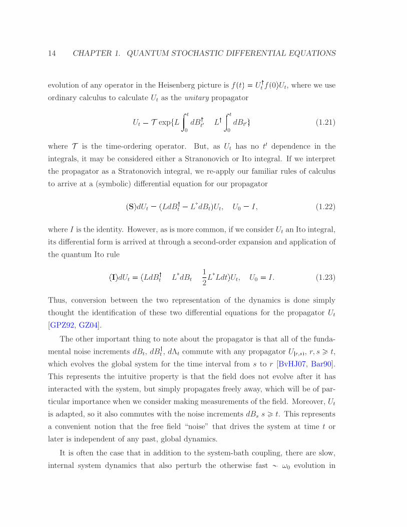
an Ito QSDE for the propagator (dropping the pIq hereon)dUt pLdB:
t L:dBt piH 1
2L:LqdtqUt, U0 I. (1.24)
Expressing the entire system dynamics, this equation of motion for the propagator is
the main object of analysis in most QSDE models [GZ04, BvHJ07, GJ09b].
You may have noticed that at no point have we “traced over the bath” in the
analysis, as is common to do in open quantum systems theory. This is because we
typically measure the bath to some extent. Before we get to the topic of measurement,
though, let’s consider what the above propagator tells us about the evolution of system
expectations when an experimenter makes no measurements.
1.3 The master equation
Say we have some system operator X and we want to calculate the evolution of its
expectation in time. The evolution of X in the Heisenberg picture is U :tXUt jtpXq.
A clearer picture of jtpXq comes from considering its differential form (using the
quantum Ito rule) [BvHJ07]. For this calculation, recall that as we are considering
Ito noise processes, the noise increments at time t are independent of the propagators
up to that point, or in other words rUt, dBts rUt, dB:t s 0. Moreover, as we are
limiting ourselves to system operators, the noise increments also commute with X .
With these, we have
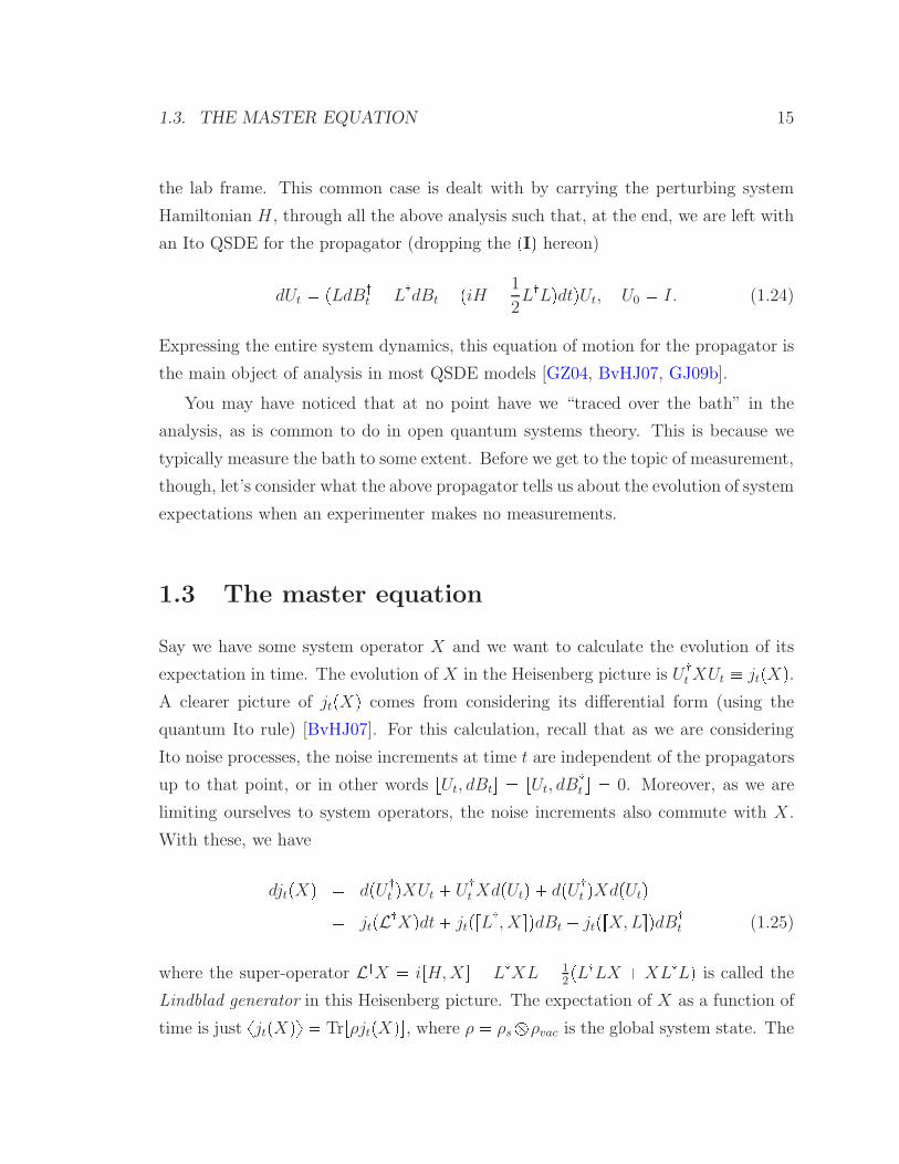
djtpXq dpU :t qXUt U
:tXdpUtq dpU :
t qXdpUtq jtpL:Xqdt jtprL:, XsqdBt jtprX,LsqdB:t (1.25)
where the super-operator L:X irH,Xs L:XL 12pL:LX XL:Lq is called the
Lindblad generator in this Heisenberg picture. The expectation of X as a function of
time is just xjtpXqy TrrρjtpXqs, where ρ ρsbρvac is the global system state. The
16 CHAPTER 1. QUANTUM STOCHASTIC DIFFERENTIAL EQUATIONS
differential form of this expectation is simply the expectation of the above QSDE.
However, this expression may be greatly simplified due to our assumption that the
bath is in the vacuum state. From our definition of the noise increments, dBt|vacy xvac|dB:t 0. Thus, the expectation of any term in the above expression for jtpXq
that contains dBt or dB:t is zero and we are left with
dxjtpXqy xjtpL:Xqydt (1.26)
which may be familiar as the master equation used in many other, non-QSDE contexts
for describing the unconditional evolution of an open quantum system [Car93a, GZ04,
Gar04].
From Eq. (1.26) and the definition of the expectation, we can also derive an
unconditional master equation for the system state in the Schrodinger picture, for use
in calculating expectations of arbitrary X :
dρuc Lρucdt (1.27)
where Lρ irH, ρs LρL: 12pL:Lρ ρL:Lq.
1.4 The series product
You may have noticed that we dropped the “input” and “output” terminology when
we moved from the “bptq” to the QSDE description. In some sense, what’s been
developed here is more flexible, but still contains that I/O intuition. For example,
consider the evolution of the noise process (using the quantum Ito rule)
djtpBtq jtpLqdt dBt (1.28)
which is equivalent to the relationship between binptq and boutptq considered above
(1.10), and is depicted in Fig. 1.1. So, if jtpBtq is the field output after interaction
with a system, can it be “fed into” another quantum system, and can QSDEs describe
this quantum network? Yes and yes.

1.4. THE SERIES PRODUCT 17
G1
G2
BS
N
Figure 1.2: An example QSDE optical network N constructed from the series andparallel connection of QSDE subsystems G1, G2, and BS: N BS G1 `G2.
Suppose the “first” system is characterized by a typical QSDE propagator, Up1qt
(Eq. (1.24)), specified by the set of coupling and Hamiltonian operators G1 pL1, H1q. A “later” system, Up2qt , is specified by G2 pL2, H2q. The process of
feeding the field, after its interaction with the first system immediately into a second
(assuming any propagation delay is much less than the dynamical timescales of the
system [GJ09a]) is modeled in the Heisenberg picture by infinitesimally propagating
any operator first by Up2qrtdt,tq and then by U
p1qrtdt,tq in infinite sequence (the Heisen-
berg picture essentially operates in “backwards” time). If we look just at the first
infinitesimal propagator [GJ09b, SSM08, GZ04]
Up2qdt U
p1qdt pI dU
p2q0 qpI dU
p1q0 q (1.29)
we can apply the quantum Ito rule to find
Up2qdt U
p1qdt I ppL1 L2qdB:
0 pL1 L2q:dB0 p12pL:1L1 L
:2L2q ipH1 H2qqdt L
:2L1dtq I ppL1 L2qdB:
0 pL1 L2q:dB0 p12pL1 L2q:pL1 L2q ipH1 H2 1
2ipL:2L1 L
:1L2qqdtq(1.30)

18 CHAPTER 1. QUANTUM STOCHASTIC DIFFERENTIAL EQUATIONS
A recursive analysis along these lines suggests that we may describe the evolution of
this cascaded system with a single propagator Up21qt propagated by the infinitesimal
increment in Eq. 1.30. More abstractly, we define a series product [GJ09b]
G21 G2 G1 L1 L2, H1 H2 1
2ipL:2L1 L:1L2q (1.31)
with its own, effective, coupling and Hamiltonian operators derived from the G1 and
G2 subsystems. Note that the consequence of putting one system after another is
essentially to couple their Hamiltonian dynamics. The ordering of the systems in the
the series is subtly encoded in the sign of this coupling term.
With this approach in hand, we revisit the question of how to model the field
produced by a laser if we are required to keep the bath in a vacuum state. First,
recall from QED that a coherent state like the output of an ideal laser may be modeled
as a displaced vacuum [WM08]. Thus, we can model a bath state with a coherent
amplitude α at times rt, 0s as|α, ty T exptα » t0
dB:t1 α: » t
0
dBt1u|vacy Wpαqt |vacy. (1.32)
From Eq. (1.32), we now have a new unitary operator called the Weyl operator that
has the differential form
dWpαqt
αdB:t α:dBt 1
2|α|2dtW pαq
t . (1.33)
If we want to analyze the dynamics of an open quantum system probed by a laser, we
can still use all our QSDE machinery by modeling the “laser” as a QSDE system that
takes the vacuum as input, displaces it by α using Wpαqt , and then feeds its output
field into the system of interest. That is, in our QSDE formalism a quantum system
interacting with the vacuum, G0 pL,Hq, is related to the same system probed by
a laser with amplitude α by [KNPM10]
Gα G0 W pαq pL α,H i
2pαL: α:Lqq. (1.34)

1.5. MULTIPLE FIELDS 19
1.5 Multiple fields
In addition to connecting systems in series, it is possible to connect them in parallel,
as depicted in Fig. 1.2. In fact, this is a more straightforward concept. We simply
assume the existence of multiple input fields, each of which must also have an output.
Physically, these fields may be any other free optical mode somehow orthogonal to the
others due to polarization, frequency, spacial mode, etc. Individual systems may also
have multiple field inputs (and an equal number of outputs). In this generalization,
each process must carry an index specifying to which mode it is associated. However,
the gauge process becomes particularly interesting in this generalization. If both biptqand bjptq are quantum noise processes, indexed to modes i and j, then we define
Λijt » t0
dΛijt » t0
dtb:i ptqbjptq. (1.35)
Because of this, gauge processes may now scatter field inputs between the outputs
(e.g. be used in the modeling of a beamsplitter). With multiple fields present, the
index of each field enters the quantum Ito table 1.1 in a straightforward manner.
We also define a more generalized propagator that evolves multiple fields, and may
describe a scattering among them [GJ09b, KNPM10]
dUt j,k
pSjk δjkqdΛjkt LjdBj:t L
:jSjkdB
kt piH 1
2L:jLjqdtUt, U0 I
(1.36)
where the scattering matrix S is necessarily unitary, and whose elements may be
system operator-valued. Thus, our set of characteristic operators for a system used
in the previous section must be expanded and generalized to be the set of operator
arrays G pÑS , ~L,Hq. As an example, a beamsplitter (which only scatters fields and
has no internal dynamics) is modeled as
BS α β:β α:
, 0, 0
(1.37)

20 CHAPTER 1. QUANTUM STOCHASTIC DIFFERENTIAL EQUATIONS
where |α|2 |β|2 1. Given this, individual QSDE components may be placed in
parallel using the concatenation product
G1 `G2 S1 0
0 S2
,
L1
L2
, H1 H2
(1.38)
The introduction of the scattering matrix also requires our definition of the series
product to be slightly modified to account for field scattering. Namely, we have
G2 G1 S2S1, L2 S2L1, H1 H2 i
2pL:1S:2L2 L
:2S2L1q (1.39)
1.6 Adiabatic elimination with QSDEs
Although the Markov approximation in section 1.1 yields a dramatically simpler (but
typically extremely accurate) description of the system-bath coupling dynamics, many
QSDE descriptions are still quite complex. In traditional quantum optics, it is some-
times appropriate to simplify open quantum systems by invoking a separation of
time-scales principle to adiabatically eliminate fast dynamical variables that do not
affect slower quantities of interest [Gar04, Sto06]. This technique has been adopted
into the QSDE literature with an algorithm that calculates an approximate propaga-
tor Ut that converges to the exact propagator Upkqt in a very strong sense [BvHS08]
limkÑ8 sup
0¥t¥T pU pkqt Utq|ψy 0, (1.40)
for all |ψy in the domain of the ‘slow’ dynamical subspace, where k is a parameter
that scales with the fast dynamical rates. The theorem that guarantees this strong
convergence assumes that the operator coefficients that define a stochastic integral of
the form Eq. (1.36) for Upkqt scale with k in a particular waypiH pkq1
2l
Lpkq:l L
pkql q: k2YkAB, L
pkq:i kFiGi, pSpkqji q: Wij . (1.41)

1.6. ADIABATIC ELIMINATION WITH QSDES 21
Define P0 as the projector onto the slow dynamical subspace, P1 the projector onto the
complement subspace, and assume that there exists a Y such that Y Y Y Y P1.
Given this scaling, and some structural domain requirements, the limit theorem is
guaranteed for an approximate propagator Ut that is also a stochastic integral of the
form Eq. (1.36) with operator coefficients [BvHS08] piH 1
2l
L:lLlq: P0pB AY AqP0, pSjiq:
l
P0WilpF :l Y Fj δljqP0
L:i P0pGi AY FiqP0, pL:jSjiq:
j
P0WijpG:j F
:j Y AqP0(1.42)
Readers familiar with the adiabatic elimination procedure common in the quantum
optics literature should see a clear parallel between the form of the approximate
dynamics derived with that approach [Gar04, Sto06] and the approximate QSDE
defined by Eqs. (1.42). This adiabatic elimination theorem has been essential in
my quantum network projects [KNPM10, KPCM11], yielding excellent approximate
models that isolate the critical dynamics we are interested in and require a simulation
space orders of magnitude smaller than that of the full physical model.
Chapter 2
Optical measurements and state
estimation
Any physical system obeys continuous time laws. The optical measurements we
make in a quantum optics lab are also continuous. Thus we gain knowledge about
the system we are measuring as it is evolving. In turn, by the postulates of quantum
mechanics, the dynamics of the system we are observing must be perturbed by our
measurement record. The continuous interplay of Hamiltonian and measurement
dynamics is naturally described in a QSDE context and is what gives the approach
much of its utility.
2.1 Optical measurement
2.1.1 Photon counting
As we interpret the bptq quantum noise objects as time-domain annihilation operator
densities on a free field (Eq. (1.7)), it is reasonable to claim that the gauge process
operator Eq. (1.13)
Λt » t0
b:ptqbptqdt (2.1)
22

2.1. OPTICAL MEASUREMENT 23
is an observable that counts the number of photons in the field over the time intervalp0, ts [Bar90, Car93a, GZ04, BvHJ07]. We can measure this operator experimentally
by shining the field on a photodetector for this time interval and then reading off the
total number of photons it received over the interval (as in the depiction in Fig. 1.1);
that they were received within the interval is the only information we have about the
arrival times of the photons. This procedure is known as photon counting.
In the Heisenberg picture, the photon counting operator evolves in time according
to the global propagator Eq. (1.36)
U:t ΛtUt jtpΛtq Y Λ
t . (2.2)
The infinitesimal increment of Y Λt is obtained by the quantum Ito rule
dY Λt dΛt jtpLqdB:
t jtpL:qdBt jtpL:Lqdt, (2.3)
and reapplying the rule, it immediately follows that pdY Λt q2 dY Λ
t [BvHJ07, GZ04].
This tells us that each infinitesimal increment is an observable with eigenvalues of
only 0 and 1, supporting the intuition that while Y Λt may count the number of photons
in an extended interval, dY Λt counts the number of photons incident on a detector
in a very small segment of time (i.e. so small that the probability of collecting¡1 photons is negligible). The expectation of this increment (in the vacuum field
state) is xdYty xjtpL:Lqydt, indicating that photon counting is useful as an indirect
measurement of the system’s L:L operator.
From the definition of Λt (2.1) in terms of the noise processes bptq it may be easily
seen that rΛt,Λss 0 for all t and s. More than this, though, due to the adaptedness
(section 1.2) of Λt, YΛt U
:t ΛtUt U :
sΛtUs for all s ¥ t. Thus, rY Λt , Y
Λs s 0 for all t
and s as well. This is the very important self-nondemolition property of photocount-
ing measurements of field outputs [BvHJ07]. This property is an expression of the
physically obvious notion that it is possible to build an experiment that counts the
photons up to time t and also counts them up to time s, and that we can speak of the
joint statistics of the results from both measurements. For example, if they didn’t
commute, a joint operator of these observables Y Λt Y
Λs wouldn’t even be an observable

24 CHAPTER 2. OPTICAL MEASUREMENTS AND STATE ESTIMATION
LO
signal
Figure 2.1: A depiction of optical homodyne detection. A signal mode is interferedwith a strong local oscillator (LO) beam on a 50/50 beamsplitter. The two out-puts of the beamsplitters are monitored with photodetectors and their photocurrentssubtracted.
(e.g. pY Λt Y
Λs q: Y Λ:
s YΛ:t Y Λ
s YΛt Y Λ
t YΛs ), and clearly couldn’t have any mea-
surement statistics. Because Y Λt and Y Λ
s commute, we can talk of these observables
having joint statistics. Similarly, it is straightforward to show that rjtpXq, Y Λs s 0 for
all s ¤ t, with X being any operator of the localized system (and thus commutes with
field observables like Λt). This is called the nondemolition property of photoncount-
ing. rjtpXq, Y Λs s 0 is not generally true when s ¡ t. The nondemolition property
will allow us to speak of future system observables as also having joint statistics with
the measurements we have already made [BvHJ07].
2.1.2 Homodyne measurement
There is another common type of optical measurement that is also naturally modeled
in the QSDE formalism. Homodyne detection consists of interfering a field signal with
a strong, co-resonant, coherent ‘local oscillator’ (LO) field on a 50-50 beamsplitter,
as depicted in Fig. 2.1. Photodetectors then monitor the two beamsplitter outputs
and their photocurrents are subtracted [Bar90, Car93a, WM93, GZ04, BvHJ07]. This
type of measurement has the effective operator
Y Wt U
:t peiφBt eiφB
:t qUt, (2.4)

2.1. OPTICAL MEASUREMENT 25
for some relative optical phase φ between the local oscillator and signal fields, defining
the quadrature of the homodyne measuremet. We can use our series and concatenation
products (sections 1.4 and 1.5), and our definition of photodetection to see why this
is a physically reasonable measurement model. Notice that we can describe this
quantum network of fields, local oscillators and beamsplitters as
Ghomo BS pG`W pαqq 1?2
1 11 1
,1?2
L α
L α
, H
(2.5)
where G pI, L,Hq is the system we seek to measure. The measurement operator
associated with our homodyne detection is now Y Λ1t Y Λ2
t which subtracts the photon
counts measured in one beamsplitter output from the other. This operator has the
increment
dY Λ1t dY Λ2
t dΛ11t dΛ22
t 1?2jtpL αqdB1:
t 1?2jtpL αqdB2:
t 1?2jtpL αq:dB1
t 1?2jtpL αq:dB2
t jtpα:L αL:qdt.(2.6)In the limit that α |α|eiφ is very large (compared to either the vacuum fluctuations
or L times them) this becomes
dY Λ1t dY Λ2
t 1?2|α|eiφjt dB1:
t dB2:t
1?2|α|eiφjt dB1
t dB2t
|α|jtpeiφL eiφL:qdt, (2.7)
which, up to a multiplicative factor of |α| and “undoing” the beamsplitter’s coherent
scattering of the fields (i.e. a simple change of free field bases) is exactly what one
gets for
dY Wt eiφdB
:t eiφdBt jtpeiφL eiφL:qdt; (2.8)
the two measurements are informationally equivalent.
Importantly, it can also be shown that homodyne detection satisfies the self-
nondemolition property and the nondemolition property. However, rY Λt , Y
Ws s 0

26 CHAPTER 2. OPTICAL MEASUREMENTS AND STATE ESTIMATIONt, s, which means that the joint statistics of homodyne and photocounting measure-
ments are ill-defined on overlapping time intervals, or more concretely, in a single ex-
periment, we can only choose one type of measurement on a given free field over a given
time interval (again, a physically sensible notion). Nor do homodyne measurements
of a given φ-quadrature commute with any other homodyne measurement of a differ-
ent quadrature over the same time interval. Also, it is straightforward to show that
in the case of homodyne measurement pdYtq2 dt and xY Wt y xjtpeiφL eiφL:qy
[BvHJ07]. Together, these properties give Y Wt the appearance of Brownian motion
(section 1.2), plus a deterministic drift determined by the coupling operators L.
2.1.3 Calculating photocurrent statistics
While it is immediately clear how to calculate the expectation of an optical measure-
ment increment xdY pW,Λqt y in the QSDE formalism, calculating the joint statistics of
measurements, e.g. xdY Wt dY W
s y, takes a bit more effort [WM93]. There are various
ways of calculating continuous measurement correlation functions, but QSDEs admit
an elegant approach based on characteristic functionals [Bar90, GZ04]. As the vast
majority of the experiments and theoretical work in this thesis utilize homodyne mea-
surements, this technique will be demonstrated for homodyne measurements alone,
and so I will drop the W superscript and write Yt as the optical measurement oper-
ator. This section is written more as an explanation of calculations presented later
in the thesis, and thus has a different motivation than the pedagogical explanation
of the QSDE formalism in the preceeding and succeeding sections. These technical
descriptions are a bit more involved.
Consider the functional [GZ04]
ΦT rks xexpti » T0
kpsqdYsuy xU :TVT rksUT y (2.9)
where kpsq is an arbitrary function of s, and dYs is the homodyne measurement
increment. Now note that for t1 ... tn T and using the functional derivative

2.1. OPTICAL MEASUREMENT 27
we get iBBkpt1qΦT rksk0
xdYt1dt
y xIt1ypiqn BnBkpt1q...BkptnqΦT rksk0 xIt1 ...Itny, (2.10)
where It may be thought of as the photocurrent operator (i.e. the rate of change
in Yt). Thus, we can use the characteristic functional ΦT rks to find all moments of
the photocurrent correlations. We can propagate Φtrks in time by first defining the
reduced characteristic operator χtrks TrbrVtrksUtρU :t s, in which ρ ρsb ρvac is the
global system state and the trace is over the bath subsystem only. It follows that
Φtrks Trsrχtrkss and χtr0s TrbrUtρU :t s (i.e. χtr0s is the reduced density matrix
at time t of the system alone). Choosing for demonstration purposes the φ 0 case
(i.e. amplitude quadrature measurement), the QSDE representation of Vtrks is thendVtrks #ikptqpdBt dB
:t q 1
2kptq2+Vtrks (2.11)
and it follows that
d
dtχtrks Lχtrks 1
2kptq2χtrks ikptqpLχtrks χtrksL:q, χ0rks Trbrρs, (2.12)
where L is the Lindblad generator from the master equation Eq. (1.27). Moreover,
note that this is a completely deterministic, ‘master equation-like’ equation of motion
for the measurement characteristic operator. Now using Eq. (2.12), we can find the
expected photocurrent at time txIty i BBkptqΦT rksk0 iTrsr BBkptqχT rkssk0 iTrs BBkptq » T0 pL 1
2kpsq2qχsrks ikpsqpLχsrks χsrksL:q ds
k0 TrsrpL L:qχtr0ss, (2.13)

28 CHAPTER 2. OPTICAL MEASUREMENTS AND STATE ESTIMATION
as well as the photocurrent correlation function (let t t1 T )xIt1Ity B2Bkpt1qBkptqΦT rksk0 B2Bkpt1qBkptqTrs T exp
"» T0
L 1
2kpsq2 ikpsqJ ds*χ0rks
k0 BBkpt1qTrsT exp
"» T0
L 1
2kpsq2 ikpsqJ ds*pkptq iJ qχtrks
k0 Trsrδpt1 tq exptLT uχ0r0s exptLpT t1quJ exptLpt1 tquJ χtr0ss δpt1 tq TrsrJ exptLpt1 tquJ χtr0ss (2.14)
where J ρ Lρ ρL:, T is the time-ordering operator and we have used the fact
that the Lindblad operator is trace-preserving. With Eq. (2.12), all higher order pho-
tocurrent correlations are similarly calculable. Although the calculations themselves
may be a bit opaque on a first read, note that the photocurrent expectation and
correlation functions have an intuitive final form. The expectation of the amplitude
quadrature photocurrent is simply the expectation of the “amplitude quadrature” of
the system, L L:, at time t. The two-time autocorrelation function is produced
by a combination of optical ‘shot noise’ (δpt1 tq) and another term that applies the
measurement jump super-operator J at time t, evolves the system unconditionally
until t1 (via exptLpt1 tqu), and then applies the measurement operator again before
finally taking the expectation. Eq. (2.14) was the basis for the theoretically predicted
photocurrent statistics used in Fig. 6.5.
Rather than consider the autocorrelation of instantaneous photocurrents, it is
more practically useful to consider the small, but not infinitesimal changes to the
measurement record over small, but not infinitesimal time intervals. This models a
realistic experimental situation where photocurrents are measured with a finite band-
width, or in our approximation, simply integrated over small time intervals p0, τ s. Theapproach adapts the above characteristic functional approach to give a 2D represen-
tation of the finite bandwidth photocurrents expected from homodyne measurements
of an arbitrary quadrature [Bar90], essentially producing a Wigner quasi-probability
2.1. OPTICAL MEASUREMENT 29
representation [WM08] of realistic photocurrent observables. This representation is
given by the function
W pβq 1
π2
»d2αeβα
:β:αΦτ pαq; Φτ pαq xU :τVτ pαqUτy;
Vτ pαq T exptαB:τ α:Bτu (2.15)
where α and β are c-numbers. Going beyond the suggestive looking construction of
W pαq, to demonstrate why this is like a W-function for homodyne measurements, we
can integrate the function over its imaginary axis:»dβiW pβq 1
π
»dαixT e2iαip 12Yτβrqy xδp1
2Yτ βrqy (2.16)
(where βi and βr are the real and imaginary components of β, etc.), which gives
the expectation of the observable that indicates whether amplitude quadrature mea-
surement yields a 2βr measurement result, in complete analogy to a Wigner func-
tion [WM08]. In much the same way, we calculate W pβq by defining a χτ pαq TrbrVτ pαqUtρU :
t s and finding its equation of motion
d
dtχτ pαq pL 1
2|α|2 J pαqqχτ pαq; J pαqχ αχL: α:Lχ. (2.17)
This means we can write
χτ pαq eτpL 1
2|α|2J pαqqχ0 eτpL 1
2|α|22iαrJi2iαiJrqχ0
Jrχ 1
2pχL: Lχq; Jiχ i
2pχL: Lχq; rJi,Jrs 0 (2.18)
where χ0 TrrUtρU :t s. Although everything thus far has been exact, and representa-
tions for time intervals p0, τ s of arbitrary length are valid, calculation of W pβq at thisstage would be highly numerical in most cases. However, if our detection bandwidth τ1 is fast enough, we should be able to ignore the internal, unconditional evolution
of the system over the sampling time of the detector and approximate Lτ 0. With
30 CHAPTER 2. OPTICAL MEASUREMENTS AND STATE ESTIMATION
this restriction in hand, we can use familiar non-commutative calculus to find
W pβq 2
πτTrsre 2
τ|τLβ|2χ0s (2.19)
which is very satisfying!
Why is this satisfying? It has an intuitive connection to the Wigner function for
infinitely strong measurements of the system operators L we are indirectly probing
with our homodyne field measurements. First, for simplicity assume we work with a
scaling such that L and τ are unitless. It can be shown that this strong measurement
Wigner function is [WM08]
Ws,strongpβsq 2
πTrre2|Lβs|2χ0s (2.20)
where the subscript s indicates units of the system “amplitude” (i.e. the range of L-
quadrature measurements). Through a simple change of variables, we can translate
Eq. (2.19) into these units:
W pβq ÑWspβsq 2
πTrre2|?τLβs|2χ0s (2.21)
which is equivalent to the strong measurement, but with ‘collection efficiency’?τ .
This can be seen by considering extending the system to include some other vacuum
mode χ0 Ñ χ0 b |vacyxvac| and taking L Ñ ?τL ?
1 τavac which also acts like
an annihilation operator on the vacuum mode. With this extension Ws,strongpβsq ismodified into Wspβq. Moreover, as we are assuming high bandwidth detection (so
that the collection efficiency τ 1), we can calculate the photocurrent’s Wigner
function representation Wspβsq directly from Ws,strongpβsq by noting that
Wspβsq 1?τWs,strongp βs?
τq 1?
1 τWvp βs?
1 τq; Wvpβsq 2
πe2|βs|2 , (2.22)
that is, the photocurrent Wigner function is simply the convolution of the strong
one with the Wigner function of a vacuum. This approach was the basis for the 2D
photocurrent representations and marginal quadrature distributions shown in Figs.

2.2. QUANTUM TRAJECTORIES 31
4.5 and 6.3.
2.2 Quantum trajectories
Photocurrent correlation functions may contain a complete description of I/O dynam-
ics, but they don’t give a visceral sense of what these optical measurements look like
on an oscilloscope. How can we construct typical measurement trajectories? At any
given time, we already know that the expectation of the next photocurrent increment
is xdYty xL L:ytdt (Eq. (2.13)) where the expectation is taken according to the
state at time t, and that pdYtq2 dt (apply the quantum Ito rule to Eq. (2.8)). With
these two facts, the spectral theorem and Levy’s theorem together tell us that the
quantity » t0
dMs » t0
xL L:ysds, (2.23)
where dMtdt is some photocurrent measurement sequence, is simple Brownian mo-
tion [BvHJ07], or in other words, that
dMt xL L:ytdt dWt (2.24)
where dWt is the increment of the Brownian motion process (a Gaussian-distributed
random variable). So far these arguments are very loose. For instance, we can’t
yet say what the state is at time t. If we have been making continuous homodyne
measurements up to t, the state is conditioned on the entire measurement sequence
up to time t, according to the postulates of quantum mechanics. The derivation of
the conditional expectation xL L:yc has been described by many other authors in
more rigorous contexts [Car93a, GZ04, GPZ92, SD81, WM93], most elegantly as a
continuous-time conditioning procedure derived from Bayes rule known as quantum
filtering [BvHJ07, vH07]. Again, a proper derivation is quite mathematical and is
framed in terms of probability rather than physical theories. Rather than simply
reiterate these derivations (which would take a long time), I feel it is more valuable
to try to offer a heuristic explanation for interested physicists.

32 CHAPTER 2. OPTICAL MEASUREMENTS AND STATE ESTIMATION
2.2.1 The stochastic Schrodinger equation
If we have a global system state that is initially |Ψ0y |ψs, vacby – the system is in
some state |ψsy and the free field that interrogates it is in the vacuum state – the
Schrodinger equation tells us that (using Eq. 1.24)
d|Ψty piH 1
2L:Lqdt LdB
:t L:dBt
|Ψty. (2.25)
Recall that from our definition of the noise increments, dBt|Ψty 0 for all t, that is,
dBt annihilates the state as it acts on the ‘incoming’ segment of the vacuum field at
time t. This means we can change the coefficient in front of dBt in (2.25) almost freely
without affecting the global dynamics. For example, it is also true that [BvHJ07]
d|Ψty piH 1
2L:Lqdt LpdB:
t dBtq |Ψty piH 1
2L:Lqdt LdY S
t
|Ψty (2.26)
where Y St B
:t Bt is the amplitude quadrature homodyne observable in this
Schrodinger picture. As every dY Ss commutes with every dY S
t (the self-nondemolition
property in section 2.1.2), these operators may be simultaneously diagonalized. The
diagonal elements of dY St are simply the possible photocurrent increments dMt at
time t. In principle any measurement increment from p8,8q is possible, but onlya narrow range of increments are reasonably probable, with a probability function
set by |Ψty. The diagonal elements are indexed by every possible entire measurement
sequence tdM0, ...dMtu.By the projection postulate, if we observe a particular measurement sequencetdM0, ...dMtu, then the state |Ψty is projected onto the subspace corresponding to
that particular sequence (generally decreasing the norm, if not re-normalized). Cor-
respondingly, for a particular measurement sequence, we may recursively construct
2.2. QUANTUM TRAJECTORIES 33
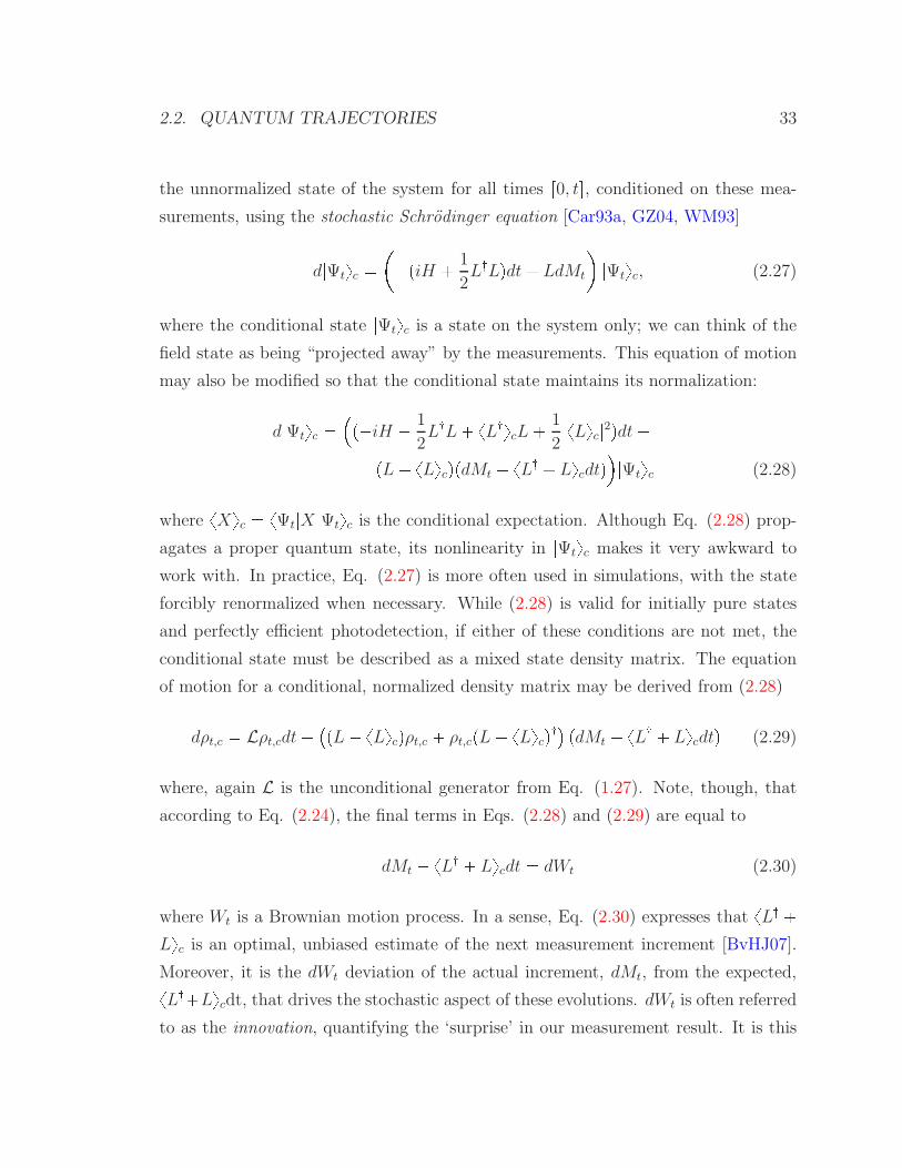
the unnormalized state of the system for all times r0, ts, conditioned on these mea-
surements, using the stochastic Schrodinger equation [Car93a, GZ04, WM93]
d|Ψtyc piH 1
2L:Lqdt LdMt
|Ψtyc, (2.27)
where the conditional state |Ψtyc is a state on the system only; we can think of the
field state as being “projected away” by the measurements. This equation of motion
may also be modified so that the conditional state maintains its normalization:
d|Ψtyc piH 1
2L:L xL:ycL 1
2|xLyc|2qdtpL xLycqpdMt xL: Lycdtq|Ψtyc (2.28)
where xXyc xΨt|X|Ψtyc is the conditional expectation. Although Eq. (2.28) prop-
agates a proper quantum state, its nonlinearity in |Ψtyc makes it very awkward to
work with. In practice, Eq. (2.27) is more often used in simulations, with the state
forcibly renormalized when necessary. While (2.28) is valid for initially pure states
and perfectly efficient photodetection, if either of these conditions are not met, the
conditional state must be described as a mixed state density matrix. The equation
of motion for a conditional, normalized density matrix may be derived from (2.28)
dρt,c Lρt,cdt pL xLycqρt,c ρt,cpL xLycq: pdMt xL: Lycdtq (2.29)
where, again L is the unconditional generator from Eq. (1.27). Note, though, that
according to Eq. (2.24), the final terms in Eqs. (2.28) and (2.29) are equal to
dMt xL: Lycdt dWt (2.30)
where Wt is a Brownian motion process. In a sense, Eq. (2.30) expresses that xL: Lyc is an optimal, unbiased estimate of the next measurement increment [BvHJ07].
Moreover, it is the dWt deviation of the actual increment, dMt, from the expected,xL:Lycdt, that drives the stochastic aspect of these evolutions. dWt is often referred
to as the innovation, quantifying the ‘surprise’ in our measurement result. It is this

34 CHAPTER 2. OPTICAL MEASUREMENTS AND STATE ESTIMATION
‘surprise’ that drives the stochastic evolution in Eq. (2.29); averaging over all possible
innovation trajectories Wt, we simply acquire the unconditional, master equation
dynamics for ρuc, as in Eq. (1.27).
Now we have a method for constructing photocurrent trajectories that we might
actual see on the oscilloscope of a quantum optics experiment, sampled from the
space of all possible measurement trajectories with the proper likelihoods. In each
time step, we first calculate the next dMt using the current ρt,c and a randomly sam-
pled value for dWt (a Weiner increment, which has a Gaussian probability density
function and generates the Brownian motion process Wt), according to (2.30). With
this same value for dWt, the conditional state ρtdt,c is updated according to (2.29).
The next photocurrent increment is then constructed in the same way, using the lat-
est conditioned state, and so on. Generalizations to imperfect detection efficiency
are straightforward (section 5.2.4 in [vH07]). Quantum trajectory simulations are
used throughout the following chapters (often using the quantum optics toolbox for
MATLAB [Tan99]), but Figs. 4.5, 6.3, and 6.5 are particularly notable for compar-
ing experimental and trajectory-simulated photocurrents with expected measurement
ensembles derived from the methods in section 2.1.3.
Any powerful set of equations has multiple interpretations, and Eqs. (2.29) and
(2.30) are powerful equations. If we have an experiment that produces a photocur-
rent trajectory tdM0, ...dMtudt, this sequence may serve as an input to Eq. (2.29),
generating a sequence of conditional states ρt,c that track the evolution of the isolated
system. This conditional state may be used to track the expectations of operators
that act on this system TrrXρt,cs πtpXq, conditioned on our measurement sequence
[BvHJ07, vH07]. This quantum filter function πtpq is optimal in the sense that, for
example, it may be used as an unbiased estimator of the next dMtdt increment, us-
ing πtpLL:q according to (2.30): πtpLL:q filters the photocurrent sequence down
to Gaussian (dWt) residuals. Quantum filtering using (simulated) photocurrents as
inputs is most directly employed in section 7.2.2.

Part II
Quantum ‘Bistability’ in Cavity
QED
35
Introduction
A two-level system (TLS) interacting with an optical resonator mode via an electric
dipole interaction has become one of the best studied quantum optical systems in the
past two decades [MD02, Car93a, TRK92, MTCK96, BMB04, EFZ07, FSS10,SBF10]. For this simple system, the sum is far richer than its parts. On its own,
an optical resonator is essentially a “classical” device: quantum mechanics may ad-
equately describe the system, but classical models also suffice unless the cavity is
driven by a non-classical field. A two-level atom is perhaps the canonical quantum
system, but in isolation, the system was completely described in the earliest decades
of quantum theory. Modern engineering has already provided us with a number of
critical technologies based on (approximate) two-level atomic spins, notably NMR
and atomic clocks. Many nonlinear optical systems may also be modeled as the inter-
action of light with atom ensembles. However, such well-known applications still rely
on ensembles of quantum mechanical spins and typically admit semi-classical models
for their interaction with electromagnetic radiation. When a single TLS couples to
an optical cavity mode with a very small mode volume, and both sub-systems each
couple weakly to all other free field modes, a fully quantum model is generally re-
quired to describe the dynamics of both the fixed (i.e. TLS and resonator) and free
field degrees of freedom, even for completely classicals input fields.
36

Chapter 3
The cQED model
This chapter introduces a standard model for cavity quantum eletrodynamics (cQED)
[MD02, Car93a] utilized in much of the remaining two parts. A single emitter with
a transition coupled to and nearly degenerate with a micron-scale optical resonator
properly requires a fully quantum I/O model to predict the evolution of its internal
states and its effect on optical probe fields. This quantum model is described, but I
also present a standard semiclassical approximation to the equations of motion. This
approximation corresponds to an analogous cQED system with many atoms coupling
strongly to the resonator in aggregate only. While the approximation fails in many
respects to describe our experimental system [KAPM11, KAM10], it is not irrelevant
and highlights the subtle dynamical transformations that occur as photonic devices
approach microscopic scales.
3.1 The cQED master equation
The Hamiltonian
We adopt the Jaynes-Cummings model [Car93a, AM06] to describe the internal,
Hamiltonian dynamics of our cQED system. Despite it’s dramatic simplifications
of any experimentally realistic system, the model captures much of what’s essential
and interesting in atom-photon interactions, and experimental realizations that best
37

38 CHAPTER 3. THE CQED MODEL
κγ⊥
g
Figure 3.1: A depiction of the cavity quantum electrodynamical (cQED) I/O system.A single, two level atom couples with rate g (per
?photon) to a single optical mode of
a resonator, here shown as a Fabry-Perot cavity. Optical free fields may drive one sideof the resonator and be transmitted through the other side via the highly reflectivemirrors. The cQED system is thus coupled to various free optical fields: the cavitymode and the input-output (I/O) free fields with cavity field decay rate κ, and theatom and transverse free fields with the atom’s electronic dipole decaying at rate γK.approximate this simplicity are often considered the most fruitful to study.
The “atom” (be it a real atom, like Cs [Ste], or a solid-state charge impurity, like
a nitrogen vacancy center [BFSB09] or quantum dot [EFZ07]) is a two-level system
(TLS), with the natural basis states ground |gy and excited |ey, so-named to reflect
their association with the atom’s electronic ground state and a single excited state.
The lab-frame energy associated with the two atomic states are 0 for the ground state
and a fraction of an aJ for the excited (corresponding to the optical range of the EM
spectrum, or several hundred THz). The single, optical cavity mode is modeled as
a quantum simple harmonic oscillator (SHO), with a harmonic spectrum that also
bestows single excitations (that is, photons) with optical energies. These models may
be derived from fundamental QED, but doing so is beyond the scope of the chapter
and is well-covered in many text books [CTDRG89, CTDRG92].
The Hamiltonians that describe the internal dynamics of the atom and cavity in
isolation are thus Ha ωaσ:σ and Hc ωca
:a, respectively, where σ |gyxe| isthe atomic lowering operator, a is the cavity annihilation operator, : the hermitian
conjugate, and ωa and ωc are the energies of the atom and cavity excitations, re-
spectively (~ 1 will be assumed throughout – except when experimental values
are needed). In addition to this, the dynamics associated with a coherent free field

3.1. THE CQED MASTER EQUATION 39
(i.e. a laser) driving the cavity may be modeled with an added Hamiltonian term
[Car93a, CTDRG92] Hd ipEa:eiω0t Eaeiω0tq, where E is a c-number with |E |2and argpEq proportional to the photon flux and phase of the laser drive, respectively,
and ω0 is the optical frequency of the drive.
The interaction between the cavity mode and atom is modeled as an electric
dipole interaction, or Hed gd E, where d is the atomic dipole operator (i.e. a
vector of Pauli-X and Pauli-Y operators in the t|gy, |eyu basis), E is electric field
operator for the cavity field, and g quantifies the rate of energy exchange between the
atom and field. However, it is common to invoke the rotating wave approximation
for cQED systems (dropping terms that produce interaction dynamics at twice the
excited state/photon energies), such that the interaction Hamiltonian simply becomes
Hi igpa:σ aσ:q, where the ‘phase’ of the interaction here is a convention and sets
a reference phase for the system [Car93a, AM06].
Putting all the terms together, the Hamiltonian that describes the internal dy-
namics of the cQED system in the lab frame is
Hlab Ha Hc Hi Hd ωaσ:σ ωca
:a igpa:σ aσ:q ipEa:eiω0t Eaeiω0tq. (3.1)
Dissipation dynamics
All experimental systems are open quantum systems [Car93a], meaning that at some
point they must interact with the many-body, “classical” systems which may (e.g.
photodetectors) or may not (e.g. brick walls) provide us with measurement results.
Measurements always perturb quantum systems, but when measurements are made
continuously, their effects become a critical aspect of the dynamical evolution. Even
if an experimenter is not dutifully measuring every free field that interacts with the
system with perfect efficiency (a practical impossibility), open system dynamics are
fundamentally perturbed from a Hamiltonian evolution.
Under fairly general conditions of a weak and Markovian interaction with a zero
temperature bath (like a freely-propagating optical field in a coherent state), the
equation of motion for a quantum system’s density matrix ρ, unconditioned on any
40 CHAPTER 3. THE CQED MODEL
measurement result, is described by the master equation (see section 1.3 and [Car93a,
GZ04])d
dtρ irH, ρs 2κDrOsρ, (3.2)
where H is the system Hamiltonian,
DrOsρ OρO: 1
2O:Oρ 1
2ρO:O (3.3)
is a superoperator describing the system’s coupling to the bath via operator O and
strength κ. Often, master equations like 3.2 are symbolically represented as9ρ Lρ (3.4)
where the Lindblad superoperator L generates the entire unconditional evolution.
In our cQED system, two different bath couplings are significant: transverse radi-
ation modes coupling to the atom (inducing spontaneous emission, for example), and
two single free field modes coupling to the cavity mode via the two high reflectivity
cavity mirrors (providing optical input and transmission channels). For interactions
with uncorrelated baths like these, the unconditional dynamics may be simply aggre-
gated, and the overall unconditional evolution in the lab frame becomes
d
dtρlab irHlab, ρs 2κDrasρlab 2γKDrσsρlab, (3.5)
where κ is the cavity field decay rate (such that each photon in the cavity leaks out
at mean rate 2κ) and γK is the atomic dipole decay rate (such that an excited atom
decays at mean rate 2γK).More convenient reference frames
The explicit time-dependence in Hlab is awkward to deal with. Consequently, it is
typical to boost our model into an interaction frame that removes these terms from
the Hamiltonian [CTDRG89, Arm09]. This is done by modeling the dynamics on the

3.2. THE QSDE REPRESENTATION 41
state
ρlab Ñ T :ρlabT ρ (3.6)
where
T eiω0pσ:σa:aqt. (3.7)
It follows from Eqs. (3.5), (3.6), and (3.7) that the unconditional dynamics in our
new frame isd
dtρ irH, ρs 2κDrasρ 2γKDrσsρ, (3.8)
where
H T :HlabT iBT :Bt T ∆σ:σ Θa:a igpa:σ aσ:q ipEa: Eaq (3.9)
where ∆ ωa ω0 and Θ ωc ω0 describe the laser drive’s detuning from the
atomic transition and cavity resonance frequencies, respectively.
While most analyses may be conveniently done in the frame of Eq. (3.8), for
computations it is often advantageous to apply yet another frame boost. Physically,
this transformation corresponds to “displacing” the cavity field by some complex am-
plitude α such that a cavity coherent state with amplitude β becomes β α. This
can be very convenient for canceling out large, DC cavity field amplitudes in simula-
tions if we are only interested in relatively small fluctuations in these amplitudes, for
example. The aptly named displacement operator [WM08, Arm09]
Dpαq eαa:αa (3.10)
induces this transformation of the frame: ρ Ñ Dpαq:ρDpαq ρα as well as a corre-
sponding transformation for the master equation.
3.2 The QSDE representation
While the master equation of Eq. (3.8) is extremely useful, it only tells part of the
story. While it represents the “average” effect of a bath on the cQED system (under

42 CHAPTER 3. THE CQED MODEL
appropriate approximations) [Car93a, GZ04], it doesn’t speak to the effect of the
quantum system on the bath fields that interact with it. If we are concerned with
the I/O dynamics of the free fields interacting with cQED devices, this is a critical
oversight!
A quantum stochastic differential equation (QSDE) representation of the the
cQED system is convenient for rolling both internal and free-field aspects of the
global system into a single, unified model. Given an initial state, the dynamics on
this global system is described by the QSDE for the propagator (see chapter 1)
dUt !?2κadA:
t ?2κa:dAt a2γKσdB:
t a2γKσ:dBt iH κa:a γKσ:σ dt)Ut, U0 I (3.11)
where dAt and dBt are QSDE annihilation processes (‘quantum noise’) on orthogonal
free field modes. As described in more detail in Part I, in the QSDE representation,
the internal cQED and external fields are on equal footing, so to speak. For example,
one may analyze the dynamics of internal variables jtpXq U :tXUt (in the Heisenberg
picture; X some cQED operator)
djtpXq jtpL:Xqdt?2κjtpra:, XsqdAt jtprX, asqdA:
t
a2γK jtprσ:, XsqdBt jtprX, σsqdB:
t
, (3.12)
where L: is the superoperator adjoint of the (Schrodinger-picture) unconditional gen-erator in equation (3.4), analogous to that in Eq. (1.26), and the dynamics of external
field outputs, e.g. jtpAtqdjtpAtq ?
2κjtpaqdt dAt, (3.13)
revealing intricate interrelations. Note that, in this system, the output field jtpAtqlooks an awful lot like a copy of the intracavity field, with added noise.
Similarly, dynamics conditioned on measurements of the free field outputs are also
naturally derived with the QSDE representation, as in section 2.2.1. For example,

3.3. THE MAXWELL-BLOCH EQUATIONS 43
we may wish to infer the internal state of the cQED system, ρc, based on amplitude
quadrature homodyne measurement of the optical field transmitted by a cQED device.
Given a photocurrent record from time 0 to t, with integralMt, the equation of motion
for the conditional state can be shown to be (section 2.2.1)
dρc Lρcdt?η?2κaρc ρca
: xa a:ycρc dMt ?η?2κxa a:ycdt (3.14)
where η is the quantum efficiency of the detection, and xyc is the conditional expec-
tation at time t. Note that when η 0, Eq. (3.14) is equivalent to the unconditional
evolution Eq. (3.8). Moreover, it can be shown that
dWt dMt ?η?2κxa a:ycdt (3.15)
is a Wiener increment (section 2.2.1), and thereby the statistics of Mt are also com-
pletely determined by the model. Thus, a QSDE approach, through Eqs. (3.14) and
(3.15) – and through the more elegant techniques of section 2.1.3 – is also naturally
suited to analyzing optical measurements.
3.3 The Maxwell-Bloch equations
As noted in section 3.2, the output fields we are interested in are roughly noisy versions
of the intracavity field. Thus, much intuition about the input-output dynamics of
cQED devices may gained by considering the equations of motion for expectations of
internal cQED operators. For example, from the master equation (3.8), we find thatx 9ay pκ iΘqxay gxσy Ex 9σy pγK i∆qxσy gxaσzyx 9σzy 2γKpxσzy 1q 2gpxσa:y xσ:ayq. (3.16)
where σz is the atomic Pauli-Z operator. Already, we see some important characteris-
tic dynamics. For example, with g Ñ 0, the intracavity field amplitude xay will decayto Epκ iΘq and the atom will decay to its ground state, xσzy Ñ 1. The coupling
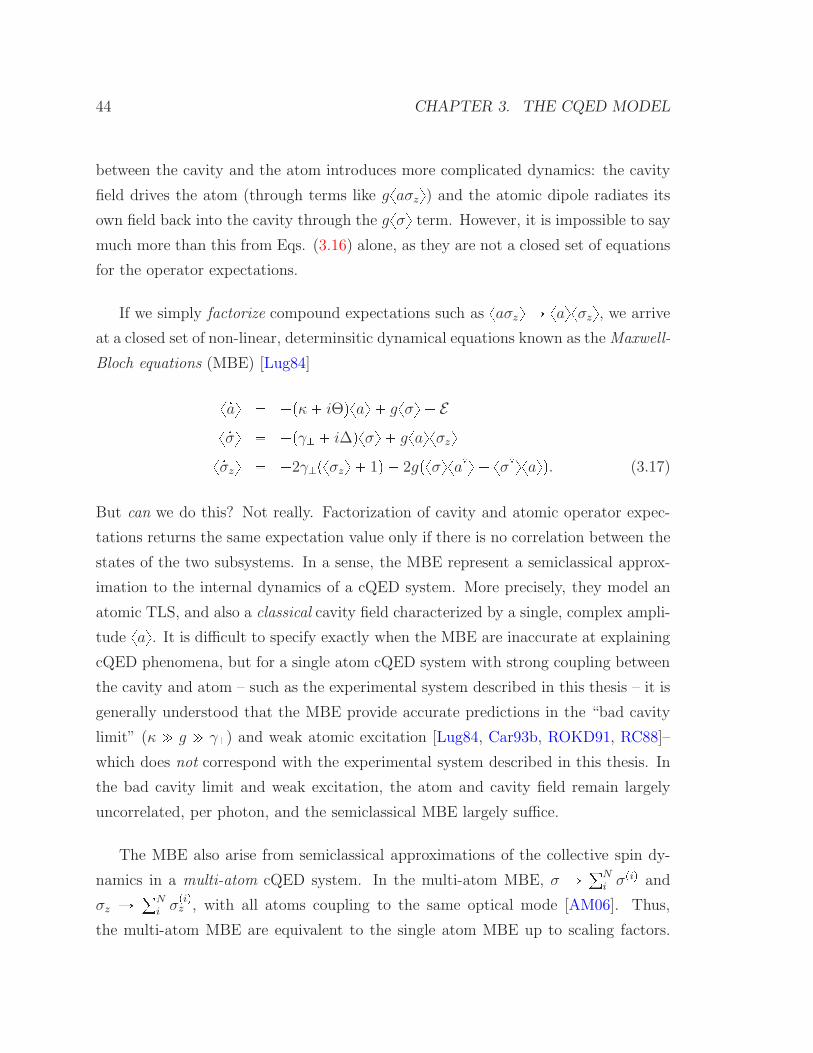
44 CHAPTER 3. THE CQED MODEL
between the cavity and the atom introduces more complicated dynamics: the cavity
field drives the atom (through terms like gxaσzy) and the atomic dipole radiates its
own field back into the cavity through the gxσy term. However, it is impossible to say
much more than this from Eqs. (3.16) alone, as they are not a closed set of equations
for the operator expectations.
If we simply factorize compound expectations such as xaσzy Ñ xayxσzy, we arrive
at a closed set of non-linear, determinsitic dynamical equations known as theMaxwell-
Bloch equations (MBE) [Lug84]x 9ay pκ iΘqxay gxσy Ex 9σy pγK i∆qxσy gxayxσzyx 9σzy 2γKpxσzy 1q 2gpxσyxa:y xσ:yxayq. (3.17)
But can we do this? Not really. Factorization of cavity and atomic operator expec-
tations returns the same expectation value only if there is no correlation between the
states of the two subsystems. In a sense, the MBE represent a semiclassical approx-
imation to the internal dynamics of a cQED system. More precisely, they model an
atomic TLS, and also a classical cavity field characterized by a single, complex ampli-
tude xay. It is difficult to specify exactly when the MBE are inaccurate at explaining
cQED phenomena, but for a single atom cQED system with strong coupling between
the cavity and atom – such as the experimental system described in this thesis – it is
generally understood that the MBE provide accurate predictions in the “bad cavity
limit” (κ " g " γK) and weak atomic excitation [Lug84, Car93b, ROKD91, RC88]–
which does not correspond with the experimental system described in this thesis. In
the bad cavity limit and weak excitation, the atom and cavity field remain largely
uncorrelated, per photon, and the semiclassical MBE largely suffice.
The MBE also arise from semiclassical approximations of the collective spin dy-
namics in a multi-atom cQED system. In the multi-atom MBE, σ Ñ °N
i σpiq and
σz Ñ °Ni σ
piqz , with all atoms coupling to the same optical mode [AM06]. Thus,
the multi-atom MBE are equivalent to the single atom MBE up to scaling factors.
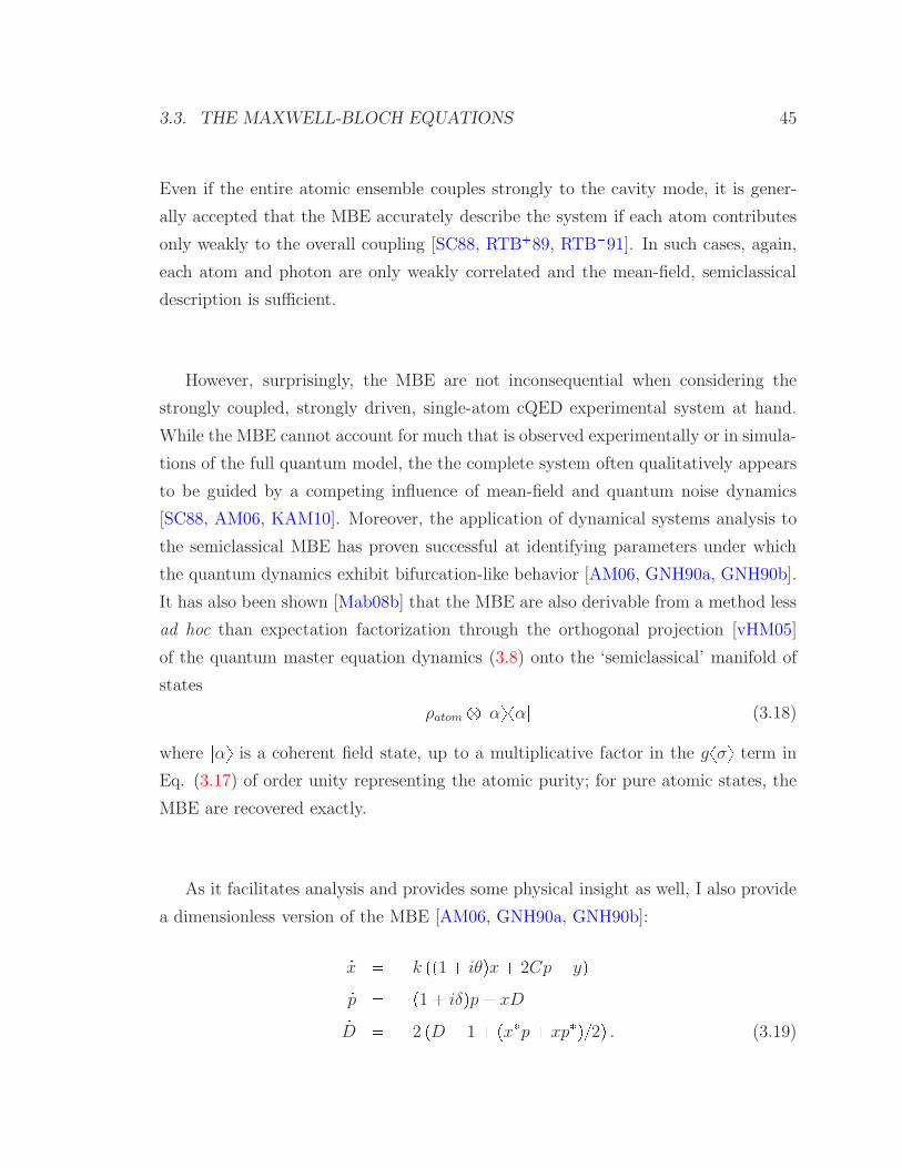
3.3. THE MAXWELL-BLOCH EQUATIONS 45
Even if the entire atomic ensemble couples strongly to the cavity mode, it is gener-
ally accepted that the MBE accurately describe the system if each atom contributes
only weakly to the overall coupling [SC88, RTB89, RTB91]. In such cases, again,
each atom and photon are only weakly correlated and the mean-field, semiclassical
description is sufficient.
However, surprisingly, the MBE are not inconsequential when considering the
strongly coupled, strongly driven, single-atom cQED experimental system at hand.
While the MBE cannot account for much that is observed experimentally or in simula-
tions of the full quantum model, the the complete system often qualitatively appears
to be guided by a competing influence of mean-field and quantum noise dynamics
[SC88, AM06, KAM10]. Moreover, the application of dynamical systems analysis to
the semiclassical MBE has proven successful at identifying parameters under which
the quantum dynamics exhibit bifurcation-like behavior [AM06, GNH90a, GNH90b].
It has also been shown [Mab08b] that the MBE are also derivable from a method less
ad hoc than expectation factorization through the orthogonal projection [vHM05]
of the quantum master equation dynamics (3.8) onto the ‘semiclassical’ manifold of
states
ρatom b |αyxα| (3.18)
where |αy is a coherent field state, up to a multiplicative factor in the gxσy term in
Eq. (3.17) of order unity representing the atomic purity; for pure atomic states, the
MBE are recovered exactly.
As it facilitates analysis and provides some physical insight as well, I also provide
a dimensionless version of the MBE [AM06, GNH90a, GNH90b]:9x k pp1 iθqx 2Cp yq9p p1 iδqp xD9D 2 pD 1 pxp xpq2q . (3.19)
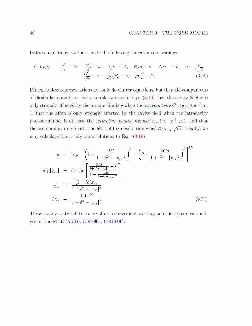
46 CHAPTER 3. THE CQED MODEL
In these equations, we have made the following dimensionless scalings
tÑ tγK, g2
2κγK C,γ2K2g2
n0 κγK k, Θκ θ, ∆γK δ, y E
κ?n0xay?
n0 x, 1?
2xσy p, xσzy D. (3.20)
Dimensionless representations not only de-clutter equations, but they aid comparisons
of dissimilar quantities. For example, we see in Eqs. (3.19) that the cavity field x is
only strongly affected by the atomic dipole p when the cooperativity C is greater than
1, that the atom is only strongly affected by the cavity field when the intracavity
photon number is at least the saturation photon number n0, i.e. |x|2 Á 1, and that
the system may only reach this level of high excitation when Eκ Á ?n0. Finally, we
may calculate the steady state solutions to Eqs. (3.19)
y |xss|1 2C
1 δ2 |xss|22 θ 2Cδ
1 δ2 |xss|2212
argrxsss arctan
2Cδ
1δ2|xss|2 θ
1 2C1δ2|xss|2
pss p1 iδqxss1 δ2 |xss|2
Dss 1 δ2
1 δ2 |xss|2 . (3.21)
These steady state solutions are often a convenient starting point in dynamical anal-
ysis of the MBE [AM06, GNH90a, GNH90b].

Chapter 4
Single atom ‘bistability’
The Maxwell-Bloch equations (MBE, Eq. 3.17) introduced in the previous chapter
represent a semiclassical description of cQED systems containing a single atom or an
ensemble of any number of atoms. Up to scaling factors, MBE describing the two
cases are equivalent. Although it’s impossible to draw a hard line between the param-
eter regimes the MBE adequately describe and those they don’t, the rule of thumb is
that they fail to capture the complete picture when individual atoms and photons are
highly correlated through strong coupling and strong driving. In these ‘deep quan-
tum’ systems, proper modeling requires a fully quantum mechanical representation.
Unfortunately, there is not yet a set of theoretical tools that generalize dynamical
systems theory to open quantum systems and one typically resorts to brute force
simulation for analysis. In other words, we don’t really understand or know what
to expect from strongly coupled, dynamical quantum systems. In particular, the a
priori relevance of semiclassical MBE dynamics to strongly-coupled cQED systems
is unclear. This thesis doesn’t resolve this uncertainty, but it demonstrates, with
experimental data, that any resolution is subtle.
This issue is not purely academic. Optical device engineering is beginning to
push into attojoule energy regime [ASO08, YHW07, LKH10, NTS10]. In the
visible to near-infrared regime, attojoule energies correspond to a countable number
of photons; e.g. one photon with an 852nm wavelength carries an energy of .23aJ.
Scientific, economic and environmental pressures are pushing information devices
47

48 CHAPTER 4. SINGLE ATOM ‘BISTABILITY’
smaller, faster and lower in energy [Mil09], and the logical consequence of this trend
is unavoidably quantum technologies. Indeed, for future optics-based processing to
be feasible, 10aJ scale devices are necessary [Mil10a], and quantum effects must
be significant if not dominant when the operating photons number in the hundreds
or less. Experimental and theoretical research has barely begun to systematically
explore this emerging engineering paradigm.
With this motivation, this chapter introduces a case study of optical I/O nonlin-
ear devices operating in the 10 photon regime that naturally arise in single atom,
strongly-coupled cQED systems. This theoretical background sets the stage for the
experiments presented in the following chapters.
4.1 Absorptive ‘bistability’
The saturable absorber is a canonical optical nonlinear I/O device. At low optical
drive powers, a medium may absorb a given fraction of incident photons, but at high
drive powers, the total power absorbed by the medium saturates. The input-output
power relationship is therefore nonlinear. Moreover, when the medium is contained
in a two-sided optical resonator and if the absorption coefficient is strong enough,
positive optical feedback from the resonator can even cause the I/O relationship to
be bistable, with either a low- or high-power transmission state possible with any
input power in a certain range [SDGK69].
This behavior can be inferred from the steady state solutions to the MBE (3.21),
with the cQED atoms in the role of the saturable medium [RTB91, AM06]. As
they become excited, the atoms scatter photons into radiation modes, dissipating the
drive power. The partially excited atoms also re-radiate their own intracavity field,
largely 180 out of phase with the optical drive, which coherently interferes with the
drive, preventing it from exciting the cavity. At high drive powers, however, the
two-level atoms become fully saturated, and the amplitude of the re-radiated field
and the rate of scattered photons no longer increase with increasing drive power. For
example, for MBE parameters (Eq. (3.20)) achievable in our single atom experiment
[KAM10], tC, n0,∆,Θu t67, .001, .7κ,1.1κu, I plot the steady-state solutions for

4.1. ABSORPTIVE ‘BISTABILITY’ 49
(a)
0.5 1 1.5 2 2.5 3 3.5
0.5
1
1.5
2
E [κ]
√n₀
|x
|ss
Steady-state intracavity amplitude vs. drive amplitude
Stable solution
Unstable solution
(b)
0.5 1 1.5 2 2.5 3 3.5
0.05
0.1
0.15
0.2
0.25
0.3
0.35
0.4
0.45
E [κ]
Steady−state atomic excitation and dipole moment
(1−D
ss)/2
|pss
|
Figure 4.1: Steady state solutions to the MBE given the parameters tC, n0,∆,Θu t67, .001, .7κ,1.1κu. (a), Steady state intracavity field magnitude,?n0|xss|, as a
function of drive amplitude E . Dynamically stable solutions are in blue, unstablesolutions in red. (b), Steady state atomic excited population, p1Dssq2, and dipolemoment, |pss|, for the same parameters. Dynamical stability again shown in blue andred.
the intracavity amplitude?n0|xss| as a function of the optical drive amplitude Eκ
in Fig. 4.1 using Eqs. (3.21). At low drive amplitudes, |E | 1.5κ, the intracavity
amplitude hardly increases with increasing drive. With increasing steady-state dipole
moment and excited state population in response to an increasing drive ampliutude,
the atoms in the MBE coherently and incoherently work to prevent field build up.
For a two-sided resonator, such as a Fabry-Perot cavity, the transmitted field is sim-
ply proportional to the intracavity amplitude and this low-|xss| state corresponds to
low optical power transmission. At high drive amplitudes, E ¡ 2.4κ, there is almost
a 1:1 correspondence between increasing drive and increasing intracavity amplitude;
consequently, nearly all the power incident on a symmetric, two-sided cavity is trans-
mitted. In this regime, atom has become completely saturated, and has no mean
dipole orientation (pss Ñ 0). The atom no longer responds to an increasing drive
amplitude, but simply scatters photons at the maximal rate of γK.Between 1.5 Eκ 2.4, however, there are three steady state solutions for any
given drive strength. The low- and high-|xss| states can be shown to be dynamically
stable, while the mid-level one is unstable [AM06]. Thus, the unstable solution serves
as a separatrix: if the system is initialized on the high- or low-side of the middle

50 CHAPTER 4. SINGLE ATOM ‘BISTABILITY’
0.5 1 1.5 2 2.5 3 3.5
0.5
1
1.5
2
2.5
3
3.5
E [κ]
Steady State Intracavity field magnitude from MBE and Quantum models
!<a
a>ss
MBE
Quantum
Figure 4.2: Steady state intracavity field amplitude solutions according to the MBEand full quantum models using the same parameters in Fig. 4.1.
solution, the system will respectively relax to the high- or low-|xss| steady state. The
MBE thus predict an amplitude bistable system for this parameter set. One dramatic
consequence is that it should be possible to adiabatically sweep the drive amplitude
from below 1.5κ to above 2.4κ and back again, and trace out a hysteretic I/O curve.
The potential use for a hysteretic input-output device like this as a robust digital
switch or for threshold signaling, has long been recognized [SDGK69, Mil10b].
But do the MBE apply in this single atom system [SC88]? To begin to answer this
question, we go back to the complete quantum mechanical master equation (3.8) from
which the MBE were derived and solve for the steady state density matrix for a cQED
system with the same parameters, over the same range of external drive amplitudes.
With these steady states, we can plot the expected magnitude of the intracavity field,axa:ayss, as in Fig. 4.2. In Fig. 4.2, rather than the same bistable response, we
see that the expected intracavity field in the full quantum model roughly “averages”
the semiclassical response, smoothly connecting the low- and high-drive regimes. In
fact, the lack of a truly bistable response is clear simply upon solving for ρss: for any
given external drive there is a unique ρss. Early single-atom cQED studies confirmed
this failure of the MBE to describe experimental single atom systems in the strong

4.1. ABSORPTIVE ‘BISTABILITY’ 51
(a) (b)
Low State High State0
0.1
0.2
0.3
0.4
0.5
0.6
0.7E =2.4κ
Low State High State0
0.1
0.2
0.3
0.4
0.5
0.6
0.7E =3κ
Low State High State0
0.1
0.2
0.3
0.4
0.5
0.6
0.7E =3.3κ
Low State High State0
0.1
0.2
0.3
0.4
0.5
0.6
0.7E =4.2κ
Low State High State0
0.1
0.2
0.3
0.4
0.5
0.6
0.7E =5.9κ
Low State High State0
0.1
0.2
0.3
0.4
0.5
0.6
0.7 E =7.4κ
P ±,e
Excited state population correlated low- and high-field states
Figure 4.3: (a), Steady state intracavity field W-functions for the same cQED pa-rameters as 4.1 and various drive amplitudes. The white cross marks the amplitudeorigin, the green circle the centroid of the W-function when the cavity is empty. (b),Excited state population correlated with the steady state low- and high-field statesfor the same parameters.
coupling regime by measuring the long-time averaged field transmitted by a Fabry-
Perot cavity containing a Cs atom [HCLK98]. But is that all there is to say about
the quantum-semiclassical correspondence?
The expected magnitude of the transmitted field is only one characteristic of
ρss. A more complete picture of the intracavity field comes when we look at the
Wigner quasi-probability functions [WM08] of each ρss after tracing over the atomic
degrees of freedom, Fig. 4.3a. As the drive amplitude is increased, in Fig. 4.3a
the intracavity field transitions from a near-vacuum state to a bimodal distribution
for 2.4 Eκ 4.2. Further inspection of ρss reveals that these lobes represent an
incoherent superposition of field states, each roughly coherent with amplitudes α 0
and α Eκ. Moreover, by projecting each ρss onto coherent field states centered
at the low- and high-lobes, we can find the excited state population associated with
each field state. To this end, in Fig. 4.3b, I plotx|α, eyxα, e|yssx|α, eyxα, e| |α, gyxα, g|yss P,e (4.1)
for each value of E in Fig. 4.3a. In Fig. 4.3b, for 2.4 Eκ 4.2, we see that
the atom in the low-field state is less than completely saturated, while the high-field

52 CHAPTER 4. SINGLE ATOM ‘BISTABILITY’
(a)
5 10 15 20 250246
⟨ X⟩ c
Expected intracavity amplitude quadrature trajectories
5 10 15 20 250246
⟨ X⟩ c
5 10 15 20 250246
⟨ X⟩ c
5 10 15 20 250246
⟨ X⟩ c
5 10 15 20 250246
⟨ X⟩ c
5 10 15 20 250246
Time [1/γ⊥ ]
⟨ X⟩ c
E = 7.4κ
E = 5.9κ
E = 4.2κ
E = 3.3κ
E = 3κ
E = 2.4κ
(b)
5 10 15 20 250246
ℜα
Amplitude quadrature photocurrent trajectories
5 10 15 20 250246
ℜα
5 10 15 20 250246
ℜα
5 10 15 20 250246
ℜα
5 10 15 20 250246
ℜα
5 10 15 20 250246
Time [1/γ⊥ ]
ℜα
E = 5.9κ
E = 7.4κ
E = 4.2κ
E = 3.3κ
E = 3κ
E = 2.4κ
Figure 4.4: (a), Quantum trajectory simulations of the conditional expectation of theintracavity amplitude field quadrature 1
2xa: ayc xXyc for the same parameters as
Figs. 4.1. (b), Simulated, 20MHz bandwidth amplitude quadrature homodyne pho-tocurrent data from the same trajectories in (a), assuming unit detection efficiency.
state is correlated with a fully-saturated atom. In contrast, the reemerging bimodality
for E ¡ 5.9κ associates a fully saturated atom with both field states, and thus has
more in common with the dispersive ‘bistability’ [AC91, AMM09, Arm09] described
in section 4.2.2. From Figs. 4.3a and 4.3b we see why the MBE fails to capture the
complete dynamics of the system (e.g. Fig. 4.2): in this near-saturation regime the
atom and cavity relax toward a superposition of highly correlated states, such that,
for example, xaσzyss xayssxσzyss. However, although the MBE steady state analysis
cannot be simply mapped onto the more accurate quantum mechanical model in this
case, the two descriptions are not completely foreign to each other. In particular, it
appears that evocative ‘remnants’ of semiclassical bistability are still retained in this
near-saturation regime: low- and high-excitation states exist in superposition in the
steady state.
But what does it mean for the steady state intracavity field to be bimodal? The
cavity can’t output a high and low amplitude field simultaneously. On a somewhat
related note, why does the long-time averaged transmitted field produce an I/O pic-
ture equivalent toaxa:ayss? These questions can be naturally addressed from the
QSDE representation of the system, as in section 3.2. For instance, from a QSDE
description, straightforward application of quantum trajectory techniques (section
2.2.1) allow us to simulate probable broadband homodyne measurements of the field
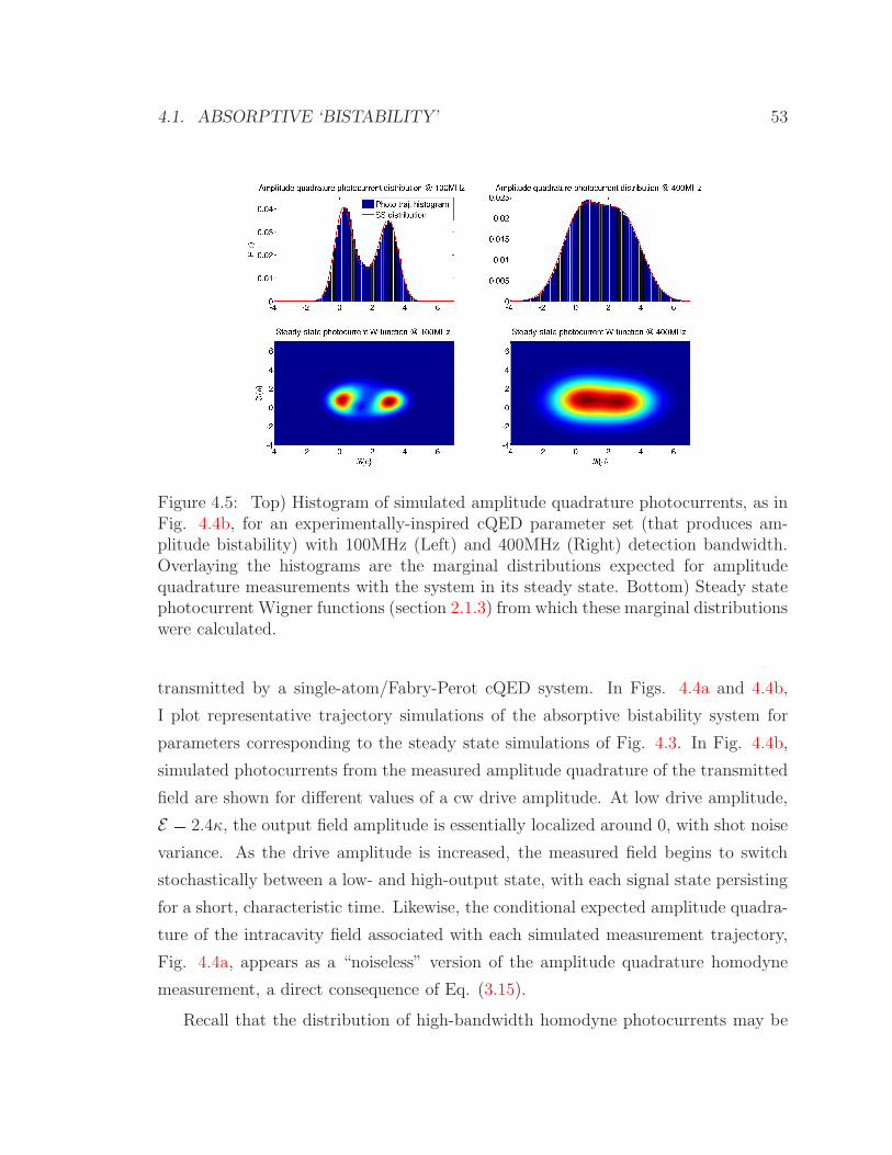
4.1. ABSORPTIVE ‘BISTABILITY’ 53
Figure 4.5: Top) Histogram of simulated amplitude quadrature photocurrents, as inFig. 4.4b, for an experimentally-inspired cQED parameter set (that produces am-plitude bistability) with 100MHz (Left) and 400MHz (Right) detection bandwidth.Overlaying the histograms are the marginal distributions expected for amplitudequadrature measurements with the system in its steady state. Bottom) Steady statephotocurrent Wigner functions (section 2.1.3) from which these marginal distributionswere calculated.
transmitted by a single-atom/Fabry-Perot cQED system. In Figs. 4.4a and 4.4b,
I plot representative trajectory simulations of the absorptive bistability system for
parameters corresponding to the steady state simulations of Fig. 4.3. In Fig. 4.4b,
simulated photocurrents from the measured amplitude quadrature of the transmitted
field are shown for different values of a cw drive amplitude. At low drive amplitude,
E 2.4κ, the output field amplitude is essentially localized around 0, with shot noise
variance. As the drive amplitude is increased, the measured field begins to switch
stochastically between a low- and high-output state, with each signal state persisting
for a short, characteristic time. Likewise, the conditional expected amplitude quadra-
ture of the intracavity field associated with each simulated measurement trajectory,
Fig. 4.4a, appears as a “noiseless” version of the amplitude quadrature homodyne
measurement, a direct consequence of Eq. (3.15).
Recall that the distribution of high-bandwidth homodyne photocurrents may be
54 CHAPTER 4. SINGLE ATOM ‘BISTABILITY’
associated with a convolution of the cavity field and vacuum field distributions, as in
section 2.1.3. If broadband photocurrents produced by an experiment or simulation
with a cw drive are accumulated for time intervals much longer than their mean corre-
lation time (see Fig. 4.3, section 2.1.3 and figure 6.4) they may be accumulated into a
histogram that matches the distribution of photocurrents expected from ρss, as in Fig.
4.5 (suggesting that the system is in a sense Ergodic). Moreover, the expected inte-
gral of these measurements approaches xYtyss t?2κxa: ayss (section 2.1.3). Thus,
if an experiment only has access to long time-averaged (low-bandwidth) records, the
inferred homodyne photocurrents of the field transmitted by a cavity simply reflect
the steady state expectation of the corresponding intracavity field quadrature, i.e.?2κxa: ayss, and may be used to directly compare the steady state semiclassical
and quantum mechanical predictions for the intracavity field, in a manner similar
to Fig. 4.2 or [HCLK98]. At the other extreme, very large bandwidth photocur-
rents correspond to very weak measurements of the instantaneous intracavity field,
and thus appear to be mainly shot noise. However, if full bandwidth measurements
are resampled at intermediate rates, only slightly faster than the bandwidth of the
photocurrent autocorrelation function, a sort of quasi-‘bistability’ response to the cw
drive is apparent in the transmitted field, randomly switching between low and high
states that correspond to the low- and high-amplitude states of the steady state intra-
cavity field, as in Figs. 4.4b, and accumulation of these photocurrents reveal bimodal
distributions as in 4.5. This insight begs the question then, if quasi-‘bistability’ is
apparent on these intermediate time scales, are other signatures of true bistability,
like hysteresis, apparent on these time scales? We will take up this question again in
chapter 6.
A loose explanation for the spontaneous switching dynamics visible in the quantum
trajectories Figs. 4.4 is that the semiclassical steady states apparent in Fig 4.1a are
‘destabilized’ by quantum fluctuations [SC88, RTB91, HCLK98]. As the low- and
high- field states are essentially coherent states in Fig. 4.3, separated by only 10photons, the quantum uncertainty in the field amplitude in either state is fractionally
large. For example, if the cQED system is in the saturated, high-field state, it doesn’t
take that long (the apparent state correlation time in Fig. 4.4b) for the statistical

4.2. DISPERSIVE ‘BISTABILITY’ 55
fluctuations in the intracavity field and atomic dipole to ‘kick’ the system into the
unsaturated, low-field state: if, by chance, a low intracavity photon number happens
to coincide with the atom being the ground state, the atom can efficiently work to
reinforce the low-field state. The MBE, however, accurately predict a truly bistable
system when the saturable medium is a strongly coupled atomic ensemble, rather
than a single atom [RTB91]. This is because although the single- and multi-atom
MBE are equivalent up to scaling factors, the photon-number separation of the low-
and high-field states scales as the number of atoms in the ensemble, greatly increasing
the fluctuation-limited correlation times of the two states [SC88]. Ensemble cQED
devices operate on much higher energy scales than single-atom devices with the same
dimensionless MBE parameters (3.20) [RTB91, SC88], in a regime where quantum
fluctuations are dynamically negligible.
4.2 Dispersive ‘bistability’
As a highly nonlinear system with many tunable parameters, it should not be sur-
prising that single atom cQED offers a wide range of interesting (and potentially
useful) I/O regimes. While the absorptive ‘bistability’ described in the preceeding
section occurs right at the cusp of atomic saturation, many nonlinear I/O systems
exist completely into the high drive regime. This perhaps runs contrary to a popular
conception that in the high-excitation regime, single-atom cQED becomes increas-
ingly ‘classical’ [HCLK98, EFF07, FSS10]. In a sense, this section complements
the previous one and illustrates that even into this ‘classical’ regime of strongly cou-
pled, but fully saturated single atom cQED, quantum dynamics are clearly apparent,
if you know how to look for them [AC91, AMM09, Arm09, KAPM11]!
4.2.1 The Jaynes-Cumming ladder
The argument for recovered classical behavior in the high-drive limit comes from
analysis of the Jaynes-Cummings Hamiltonian Eq. (3.1). Minus the external drive
term, the spectrum of energies associated with the lab-frame Eq. (3.1) for a resonant
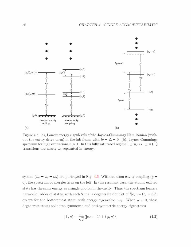
56 CHAPTER 4. SINGLE ATOM ‘BISTABILITY’
(a)
|–,1〉
|+,1〉
|–,2〉
|+,2〉
|g,0〉
|g,1〉,|e,0〉
|g,2〉,|e,1〉
|g,0〉
2g
2g√2
no atom-cavitycoupling
atom-cavitycoupling
ω0
ω0 ω0
ω0
(b)
|–,n〉
|+,n〉
|–,n+1〉
|+,n+1〉
ω0
ω0
2g√n+1
2g√n
Figure 4.6: a), Lowest energy eigenlevels of the Jaynes-Cummings Hamiltonian (with-out the cavity drive term) in the lab frame with Θ ∆ 0. (b), Jaynes-Cummingsspectrum for high excitations n " 1. In this fully saturated regime, |, ny Ø |, n1ytransitions are nearly ω0-separated in energy.
system (ωa ωc ω0) are portrayed in Fig. 4.6. Without atom-cavity coupling (g 0), the spectrum of energies is as on the left. In this resonant case, the atomic excited
state has the same energy as a single photon in the cavity. Thus, the spectrum forms a
harmonic ladder of states, with each ‘rung’ a degenerate doublet of t|e, n1y, |g, nyu,except for the bottommost state, with energy eigenvalue nω0. When g 0, these
degenerate states split into symmetric and anti-symmetric energy eigenstates|, ny 1?2p|e, n 1y i|g, nyq (4.2)

4.2. DISPERSIVE ‘BISTABILITY’ 57
Figure 4.7: The fractional optical power transmitted by a Fabry-Perot cavity con-taining a resonant strongly coupled TLS at various drive powers. The n drive powerindex refers to the number of photons that would be in an empty cavity on resonance.Taken from [Arm09].
with energy eigenvales E,n nω ?ng. Thus, for n ¥ 1, the energy eigenstates
are associated with a fully saturated atom (xσzy 0). However, an additional atom-
and-cavity “saturation regime” exists very high up, when n " 1. At these levels in
the energy spectrum, see Fig. 4.6b, the energy separation between eigenstates with
the same orientation approaches
E,n1 E,n ω0 g?
n 1?n ω0 g
2?n. (4.3)
As n Ñ 8, the spectrum of energies approaches that of a pair of harmonic ladders,
with raising/lowering energy ω0.
Adding drive dynamics to this picture provides the necessary energy to access
these high energy states, and dissipation dynamics cause the system to stabilize in
some energy regime. Moreover, the spontaneous decay of photons out of the cavity,
through the mirrors, and atomic spontaneous emission into radiation modes, broadens
the energy eigenstates of the Hamiltonian model such that each has an intrinsic

58 CHAPTER 4. SINGLE ATOM ‘BISTABILITY’
linewidth Γ maxtκ?n, γKu. When an external laser also at frequency ω0 is used to
drive the cavity when g " Γ, the cQED system cannot easily absorb the energy quanta
necessary to work its way up the first few rungs of the Jaynes-Cumming spectrum;
photons from the laser drive are not resonant with any allowed energy transitions
(to within their linewidth). However, a laser tuned to ω0 g will resonantly excite a
ground state system to |, 1y, but again cannot easily drive the transition to |, 2y.But once an ω0 laser does manage to off-resonantly excite the cQED system to the|, 2y state, all subsequent transitions to higher energy states become increasingly
resonant with the drive. If the cQED dissipation rates are slow, such that for a
g 0 system, a strong, on-resonant drive yields the steady state expected intracavity
photon number xa:ayss |Eκ|2 " 1, then even with a strongly coupled, g " Γ
single atom in the cavity, the steady state xa:ayss Æ |Eκ|2. Consequently, if the
optical drive strength is weak, the steady state power transmitted by a Fabry-Perot
cavity reveals a bimodal spectrum, with peaks at ω0 g, but if the drive is strong, a
single transmission peak is observed at ω0, as in Fig. 4.7. This ‘recovered’ harmonic
spectrum at high drive strengths would seem to suggest that highly excited single-
atom cQED systems are essentially classical objects, like any SHO [FSS10].4.2.2 Phase ‘bistability’ in highly-excitated cQED
However, even in the on-resonant, fully saturated regime of cQED with a cw laser
drive, the I/O field relationship carries clear signatures of the quantum mechanical
nature of the atom-cavity system [AC91, Arm09]. A heuristic, but remarkably accu-
rate [AC91, Arm09], explanation for this phenomenon comes from first noting that in
steady state with strong drives, the intracavity field is in some coherent state (this is
also suggested by the harmonic spectrum). Although the steady state system is not
in a photon number eigenstate, or even an energy eigenstate, the intracavity energy
distribution is centered at some ω0n, with width ω0
?n. This corresponds to a
population distribution amongst the |, n?ny energy eigenstates. The separation
in energy between ‘+’-oriented eigenstates is then ω0 g
2?n?n ω0 g
2?nand
the ‘-’-oriented eignenstates are split by ω0 g
2?n.

4.2. DISPERSIVE ‘BISTABILITY’ 59
We can then approximate this cQED system about the steady state as two, offset
SHOs with resonant energies ω0 g
2?n. As our optical drive is tuned to ω0, and is
thus slightly off-resonant with either SHO system, the intracavity optical dynamics
largely satisfy x 9ay κ ig
2|xay| xay E (4.4)
where xay is the intracavity field expectation associated with each, independent SHO
sub-system (compare with the MBE (3.17)). The steady state solutions to Eq. (4.4)
are
αss xay,ss E
κ
1 g
2E
2 ig
2κ
1 g
2E
2
, (4.5)
and as g
2EÑ 0, xay,ss E
κ ig
2κ. Thus the intracavity field will have a slight phase
shift dependent on which SHO ladder the system is localized on, the ‘+’ one or the ‘-’
one. Note that the existence of only two SHO systems can ultimately be traced to the
binary states of the atom. If the atom had more states, or if there was more than one
atom, there would be several or many more available levels in the energy spectrum,
which would eventually ‘wash out’ the digitization of the steady states xay,ss. The
intracavity ig
2κphase shift consequently results in a potentially observable positive
or negative phase shift in the field transmitted by a Fabry-Perot cavity.
So which phase state will the cQED system be in? As the system is completely
symmetric, the answer is, again, ‘both.’ But again, the cavity can’t simultaneously
transmit both types of fields. The open dynamics efficiently decoheres any quantum
superposition between the two intracavity coherent states. As in the case of single
atom absorptive ‘bistability,’ we can plot Wigner functions of the steady state intra-
cavity field for an on-resonant cQED system with increasing optical drive, see Fig.
4.8. As expected from the heuristic, semiclassical model Eq. (4.5), these fully quan-
tum mechanical simulations show a bimodal field distribution emerging in the phase
quadrature of the intracavity field as Eg increases beyond .5, with the separation
saturating at i gκ. Again, it can be shown that the steady state in the full saturation
regime is an incoherent mixture of the SHO steady states,
ρss 1
2
|, αssyx, αss| |, αssyx, αss| . (4.6)

60 CHAPTER 4. SINGLE ATOM ‘BISTABILITY’
Figure 4.8: Steady-state intracavity field Wigner functions for tg, κ, γK,Θ,∆u 2π t56.8, 9.3, 2.6, 0, 0uMHz and variable cavity drives E . The green circle denotesthe W-function centroid for an empty cavity for each drive case. Note that the realaxis changes for each plot.
As photon counting destroys any optical phase information, if one simply measures
the transmitted power in such a cQED system, as in Fig. 4.7, the cavity appears to
simply transmit a coherent field with amplitude|αss| E
κ
1 g
2E
2
, (4.7)
which approximates the empty cavity transmission in the high-drive limit.
Phase quadrature optical homodyne measurements reveal far more interesting dy-
namics, however [AC91]. As with the absorptive ‘bistability’ dynamics, the answer to
the question “which phase state will the cQED system be in” is essentially “sometimes
one, sometimes the other.” The rate at which these transitions happen on average
is γK2, which can be traced to the following physical picture. We have not yet ad-
dressed the role of atomic spontaneous emission in these phase ‘bistable’ systems.
As the atom is fully saturated in the strong driving regime, it will spontaneously
emit photons with an average rate of γK. With each emission event, the atom falls
into the ground state and one excitation (out of many) is lost from the system. The
still-strong field inside the cavity will again work to saturate the atom, but with a
4.3. TOWARD OPTICAL CONTROL 61
random polarization-orientation; half of the time the atom will reorient itself in the
‘’ state, half of the time in the ‘’ state. Thus the intracavity field, and the field
transmitted by the cavity will switch randomly between the two possible phase states
with mean rate γK2. Although the random, digital switching between two coherent
states in these phase ‘bistable’ systems (e.g. Fig. 4.9) may appear equivalent to the
behavior of the amplitude ‘bistability’ system (e.g. Fig. 4.4b) at first glance, it should
be emphasized that the system parameters, the underlying physical mechanisms, and
the energies associated with both flavors of ‘bistability’ are quite distinct.
4.3 Toward optical control
The existence of a ‘bistable’ response to an optical input is necessary to motivate single
atom cQED systems as a potential paradigm for ultra-low energy optical signaling
devices. That these systems switch between the two possible states spontaneously due
to quantum fluctuations in the cavity and atomic dipole is convenient for experimental
demonstration that both states exist and is a fundamental issue for low-energy devices,
but uncontrollable dynamics are usually useless. Some external, preferably optical,
control of the signaling state would be critical in any engineering application.
To this end, we have made some initial attempts to control the switching dynam-
ics of the phase ‘bistability’ system, as described in [KAPM11] and section 6.2. The
origin of the phase bistable phenomenon depicted in Fig. 4.6b suggests an intuitive
strategy for external control of the system’s phase state. By driving the cavity with
an additional laser beam tuned resonant with the |, ny Ø |, n 1y transition, oneshould be able to externally drive transitions between the two phase states. Such a
strategy is attractive in its simplicity, but there are several problems with it. For
instance, applying a full ‘bit-flip’ to the I/O state would depend on a carefully timed
optical pulse, with the required pulse length fairly sensitive to drifts in the system
parameters. Moreover, driving transitions between the two dispersive states coher-
ently (i.e. with the additional laser) works in direct competition with the dissipative
dynamics that enforce the digitization of the I/O response. On both counts, a more
elegant approach would be to incoherently “draw out” photons that would induce

62 CHAPTER 4. SINGLE ATOM ‘BISTABILITY’
the desired transition. An additional optical cavity tuned to ω 2?ng surrounding
the atom would do precisely that: a system in the |, αssy state would tend to emit
photons into the additional cavity mode, relaxing the system into the |, αssy state,where it would stabilize. Unfortunately, building a second cavity is not a realistic
experimental option (yet). Whereas adding another laser drive is a relative piece of
experimental cake.
In the next subsections, I lay out a partial theoretical analysis for the dynamics
associated with simply adding an additional ω2?ng tuned control beam to a phase
‘bistability’ system. Not only does this analysis introduce an alternative approach to
analyzing single atom cQED quantum dynamics using hybrid-Wigner functions, it is
hoped the analysis will aid future efforts to find more sophisticated optical control
techniques.
4.3.1 Driven transition dynamics
We model our controlled phase bistability system by adding a second cavity driving
term to the Hamiltonian, representing a second, control laser at a distinct optical
frequency:
H2 ωca:a ωaσσ igpa:σ aσq iεpeiωpta: eiωptaq
ipεceiωmta: εceiωmtaq (4.8)
where ωp is the frequency of the ‘probe’ laser, ε is its amplitude (chosen to be real, by
convention), ωm is the frequency of the ‘control’ laser with amplitude εc. As usual,
we transform the reference frame to remove the time dependence in the probe driving
term of the Hamiltonian using the transformation operator
Tt eiωpta:aeiωptσσ, (4.9)
which transforms the Hamiltonian as T :HT i BBt pT :qT to give
H 1 Θa:a∆σσ igpa:σ aσq ipε εceiΦtqa: ipε εceiΦtqa (4.10)

4.3. TOWARD OPTICAL CONTROL 63
where Φ ωm ωp is the residual rotation frequency of the control drive. The
dissipative cavity decay and spontaneous emission dynamics are not affected by this
transformation and are represented in a master equation by
DrCsP C:PC 1
2C:CP 1
2PC:C (4.11)
using Cc ?2κa and Ca ?
2γKσ terms. We will assume Θ ∆ 0 for the
remainder of this section. We will further displace the expected system mean field
α εκ with
Dpαq eαa:αa (4.12)
so that we again have a new, effective Hamiltonian
H igpa:σ aσq ipεceiΦta: εceiΦtaq iΩpσ σq (4.13)
where Ω gεκ. We transform the dynamics yet again into a iΩpσσq interactionpicture,
TΩ eΩpσσqt eiΩσyt, (4.14)
such that
T:ΩσTΩ i
2pµe2iΩt µz µe2iΩtq (4.15)
where the µ’s are essentially the raising and lowering operators in the Pauli-y basis:
σy|y |y, µ |yx|, µz σy. With this final transformation, the Hamilto-
nian becomes
HPB gXµz igY pµe2iΩt µe2iΩtq iεcpeiΦta: eiΦtaq (4.16)
where X 12pa a:q, Y i
2pa: aq. Normally, when εc is not present, the rotating
wave approximation is invoked at this point to omit the time dependent Hamiltonian
terms. The dissipative dynamics are unaffected by this final transformation, and after
the rotating wave approximation we are left with 2κDrasρ, γK2pDrµs Drµzs Drµsqρ decay processes. For much of the rest of this analysis we will set γK Ñ 0
to simplify the generally much faster dynamics we are concerned with. It’s hard

64 CHAPTER 4. SINGLE ATOM ‘BISTABILITY’
to pinpoint the effect of εc on the familiar phase ‘bistability’ dynamics. However,
a number of clues about its significant effect when Φ 2Ω can be found through
analysis and supported by simulation. Roughly, when this resonance condition is met,
the modulation of Y at frequency Φ by the final term in Eq. 4.16 results in ‘slow’
dynamics in the atomic dipole due to the ‘2Ω’ coupling term in the Hamiltonian
that is usually ignored. Intuitively, this ‘control’ drive is tuned to excite coherent
population transfer between the |, ny Ø |, n 1y states of the system. How well it
can achieve this, though, is limited both by the ‘measurement’ of the |, ny ‘dressedstate observable’ through cavity decay and the distribution of system population at
any given time over various ‘rungs’ in the phase bistability eigenenergy ‘ladder.’ I
attempt to understand these effects through divide and conquer: first tackling the
‘measurement’ of the system state through cavity decay without any control drive,
and then isolating just the control dynamics to gain some intuition of how well they
perform even without this decoherence process.
4.3.2 Dynamics without control
We will now shift to a Wigner function representation of the cavity state with the
hope that it will lead to a more physical picture of the dynamics (e.g. something that
appears like a Fokker-Planck equation). Thus, the system state will now be described
as a hybrid object:
ρpαq 1
π2
»d2βeβ
αβαTrcrρDpβqs (4.17)
where ρpαq is a density matrix of the atom only, Trcrs is a partial trace over the
cavity field and Dpβq is the displacement operator of coherent amplitude β, and
d2β dpℜtβuqdpℑtβuq. By writing the evolution of ρpαq due to the cavity operators
as partial differential operators on Dpβq (e.g. a:Dpβq BBβ β2
Dpβq) the cavity
master equation dynamics may be turned into a differential equation for the Wigner
representation [WM08]BBtρpαq BBαpκα εceiΦtq BBα pκα εceiΦtq κ
B2BαBα ρpαq. (4.18)

4.3. TOWARD OPTICAL CONTROL 65
Similarly, if we look at the dynamics that couple the field to the atomic dipole in Eq.
4.16 we get (ignoring terms that oscillate at 2Ω)BBtρpαq i
4g
BBα BBα tµz, ρpαqu i
2gpα αq rµz, ρpαqs (4.19)
where t, u is the anticommutator and r, s is the commutator. So that if we ignore
spontaneous emission and the control beam, we have the master equation dynamics
on this representationBBtρpαq BBαi pκαiρpαq g
4tρpαq, µzuq BBαrκαrρpαq igαrrρpαq, µzs
κ
4
B2Bα2r
B2Bα2i
ρpαq (4.20)
From Eq. 4.20, note thatBBtxµe2ig
καry g2
κxµe2i
g
καry
(4.21)
That is, the expectation of µe2ig
καr decays exponentially at the rate g2
κ. It can be
shown that this operator is simply µDpi gκq in the usual representation (and it’s
operator evolution is of course the same), but it was easier to identify this observable in
Wigner representation. When the system (in this displaced frame) is in the subspace
spanned by the states |,igκy, the expectation of this operator and its Hermitian
conjugate are the off-diagonal matrix elements of the density matrix. If we are to use
these off-diagonals to coherently rotate the system between |y, then we expect to
want κ ¡ g so that these state coherences are long-lived. Note, too, that in the κ " g
limit, µDpi gκq µ, clarifying the dynamics we’re interested in yet further.
66 CHAPTER 4. SINGLE ATOM ‘BISTABILITY’
4.3.3 Control dynamics
The ‘control’ aspects of the Hamiltonian consist of those terms rotating at 2Ω in our
frame:
Hc igY pµeiΦt µeiΦtq ipεceiΦta: εceiΦtaq (4.22)
where we have set 2ΩÑ Φ. To analyze these control dynamics, we rotate the system
into the control beam frame with T exppiΦa:atq so that
H 1c Φa:a g
2paµ a:µq ipεca: εcaq (4.23)
after we ignore all terms rotating at Φ. It is still convenient to analyze the dynamics
in this frame as the atomic operators remain unaffected by the transformation. Note
that that we have recovered a familiar cQED Hamiltonian with atom-field coupling
Eq. (3.9). The cavity is effectively off resonant with the drive, though, by Φ. The
equations of motion for the principle cQED operators are9a iΦa ig
2µ εc κa9µ ig
2aµz9µz igpaµ a:µq (4.24)
We apply the familiar semiclassical approximation (section 3.3), and replace a Ñz, 2µ Ñ v, µz Ñ m to represent the (factorized) operator expectations in the equa-
tions above. Solving for steady state, we get
z 0
v 4iεc
g
m 1 |4εcg|2 (4.25)
when |εc| g4. The limit for large control amplitude may be solved in this semiclas-
sical approximation, but other than the solution m 0, the steady state expectations
are quite messy and probably not very useful as the semiclassical approximation is
4.3. TOWARD OPTICAL CONTROL 67
not appropriate in this limit. Although it doesn’t really apply in the simulations I’ve
tried, however, the perturbative control amplitude limit is useful as it suggests that
the phase of the control amplitude is unimportant and that the control should be able
to drive complete inversions of the atomic dipole as long as it is faster than g (in the
limit of very slow spontaneous emission). The suggestion of this analysis is also that
a large?κg is preferred (so that a larger inversion per external control wattage is
achieved), which is consistent with the conclusions of the no-control dynamics section
4.3.2.
4.3.4 Simulation of a controlled quantum dot system
The principle insight from the immediately preceeding sections is that the additional
ω 2?ng laser only efficiently transfers population between the two phase states if
gκ is small. At first glance, this may seem completely contrary to the regime of
‘good’ phase bistability. For example, if gκ 1, the bimodality in Fig. 4.8 would
be impossible to see. However, these figures aren’t very relevant in this context. For
example, any coherent state is perfectly distinguishable, given an infinite integration
time. What ultimately limits the visibility of a phase bistability system is the cor-
relation time of the phase states, i.e. 2γK, recall Eq. (2.14) and Fig. 4.4b. Thus,
simple arguments suggest that the visibility of a phase bistability system essentially
scales as g?κγK9?C; two cQED systems with different tg, κ, γKu parameters, but
similar cooperativities C should yield phase bistability systems with similar visibility.
In this light, the world of nanophotonics looks particularly appealing. Solid state
cQED systems typically feature extremely small mode volumes and broad cavity
linewidths, relative to what’s achievable in gas-phase cQED systems. For instance, a
photonic crystal cavity containing a single quantum dot demonstrated in the Vuckovic
group [FMK10] features a parameter set of tg, κ, γKu 2π t20, 40, .1uGHz, which
has a comparable cooperativity as our Cs/Fabry-Perot system, but with g κ.
In quantum trajectory simulation we can straightfowardly try the intuitive optical
control strategy of adding a ω 2?ng cw laser that should simply increase the mean
rate at which transitions between the two phase states occur.

68 CHAPTER 4. SINGLE ATOM ‘BISTABILITY’
0 1 2 3 4 5 6 7 8 9 10−0.5
0
0.5
Ph
oto
curr
en
t [g
0/2
κ]
Simulated photocurrent for Qdot system with 11 μW signal
0 1 2 3 4 5 6 7 8 9 10−0.5
0
0.5
Time [1/γ⊥]
Ph
oto
curr
en
t [g
0/2
κ]
Simulated photocurrent with added .27 μW control beam
a
b
Figure 4.9: (from [KAPM11]) (a) Simulated photocurrent segment assuming cQEDparameters demonstrated by [FMK10], a 11µW probe with perfect detection ef-ficiency with a 10GHz detection bandwidth. (b) Simulated photocurrent segmentassuming the same system, plus a .27µW cw ‘control’ beam detuned by a the mag-nitude of the quantum dot-mode coupling Hamiltonian, i.e. by -400GHz relative tothe probe beam.
The results of this simulation are seen in Fig. 4.9 [KAPM11]. With no control
beam present, simulated phase-quadrature homodyne measurements portray a normal
phase bistable system with switching at rate γK2. Although gκ 1 in this
system, the relatively slow atomic decay allows the photocurrent to be aggressively
low-passed (here at 10GHz) such that the difference in phase mean of the two states
is clearly visible. When a cw control beam with less than 2.5% of the optical power of
the signal probe beam is added, the spontaneous switching rate clearly increases by
roughly an order of magnitude. Although neither phase state is actually stabilized, if
the signaling state is instead defined as the rate of spontaneous phase switching, we
can define-our-way-to-success by this simulated demonstration of a controlled ultra-
low energy optical device that exploits a single two-level atom to produce a digital
I/O response.
To give a sense of the energy scales involved here, an 11µW probe corresponds
to roughly 100 intracavity photons, or a 20aJ intrinsic energy scale. More simple
calculations show that the energy dissipated in the control beam (out of every control

4.3. TOWARD OPTICAL CONTROL 69
photon incident on the cavity) per induced switching event falls in the 100aJ/edge
regime, right at the current state of the art for controlled nanophotonic switching
devices [ASO08, YHW07, LKH10, NTS10]. However low, 100aJ is still almost
three orders of magnitude above the apparent, single-photon (sub-aJ) energy differ-
ence between the phase states. The experimentally difficult (but conceptually elegant)
detuned-cavity approach to “drawing-out” single photons to stabilize desired phase
states confirms that much more energy efficient approaches to controlled and quan-
tum nanophotonic devices exist in principle. It is hoped and expected that more
sophisticated techniques such as pulse-shaping could help bring all-optical control to
cQED devices like these down to this “natural,” single-photon limit.

Chapter 5
The broadband cavity QED
apparatus
An experiment was built to realize a strongly-coupled single-atom cQED system that
could be driven at and beyond the point of atomic saturation and the field transmitted
by the cavity monitored with broadband homodyne detection. The vast majority
of the apparatus was inherited from Michael Armen’s thesis work [Arm09], himself
building upon a less specialized laser-cooling setup built by Anthony Miller.
In the experiment, a cloud of laser-cooled (but still thermal) Cs atoms are dropped
onto a high-finesse Fabry-Perot cavity that is actively stabilized to be resonant to
optical drives close in frequency to the D2 line in Cs [Ste]. The Cs cloud is diffuse
enough, and the fundamental cavity mode a small enough target that as the cloud
free-falls past the cavity only single atoms interact with the mode. Weak, off-resonant
optical probing and optical heterodyne detection of the transmitted field is used to
detect when an atom is near-maximally coupled to the cavity mode. Upon detection,
the optical probe is immediately shifted to a frequency and amplitude appropriate
to drive the system into its saturation regime and observe the dynamical response of
the transmitted field.
70

5.1. THE ATOM 71
5.1 The atom
There’s no such thing as a two-level atom, but we have a nice little alkali that can
approximate one pretty well: 133Cs, the only stable isotope of cesium. With a nuclear
spin of 7/2 and a single valence electron, the lowest hyperfine electronic states have
the valence electron in an S orbital, with total angular momentum quantum numbers
F 3 and F 4. Our experiment attempts to target a single optical transition
from one Zeeman magnetic sub-level in this ground state manifold to another single
Zeeman sub-level of a low-lying electronic excited state. Specifically, we attempt to
isolate the p6S12, F 4, mF 4q Ø p6P32, F 1 5, mF 5q transition using a
near-resonant, circularly polarized optical probe with a wavelength of roughly 852nm.
This transition is an atomic cycling transition, meaning that a properly tuned and
polarized cw probe will rapidly drive an atom initialized anywhere in the F 4
hyperfine ground state manifold to themF 4 state, where it will then continuously
cycle between the p6S12, F 4, mF 4q Ø p6P32, F 1 5, mF 5q ground and
excited states. Imperfect optical polarization and (to a lesser degree) fluctuating
magnentic fields can cause the atom to explore different states within the F 4 and
F 1 5 manifolds. For our purposes here, this is problematic as each ground and
excited state has a different coupling strength to a given optical drive, and can even
cause the atom to be optically pumped into the ‘dark’ F 3 ground states, where
it is effectively lost to the experiment. Thus, maintaining full control of the optical
polarization inside our cavity was a high priority in the experimental construction.
A nice thing about working with real atoms is that they are all the same. This is
not the case with any solid-state ‘atom’ in a photonic or superconducting microwave
system. The solid state atoms can be fairly tunable and stay put, but are also frus-
tratingly inconstant and are only partially understood [TMH08, PLZY08, HKD09].You know what you get with Cs. Gas phase atoms are also attractive in quantum op-
tics for their spectrally narrow near-IR transitions; the lines are narrow in large part
because these gas-phase neutral atoms interact only weakly with their environment.
The transition utilized here has an excited state lifetime of 30.4ns, or, equivalently,
a mean excited state decay rate of 2γK 2π 5.2MHz. The main trade-off with

72 CHAPTER 5. THE BROADBAND CAVITY QED APPARATUS
(a) (b)
Figure 5.1: (a) Schematic of the Fabry-Perot cavity assembly, down to the first levelof the vibration isolation stack. The shear mode piezo plates between the Al mountsand Al block are not shown and the separation between the high reflecting mirrorsurfaces (HR) is greatly exaggerated. (b) Photo of the experimental cavity in theUHV chamber, on the multi-level (and gold-plated) vibration isolation stack.
working with an atomic system with such nice coherence properties is that Cs (and
any neutral atom) requires bulky, complicated, and fussy vacuum and laser cooling
systems just to put the atoms where we want them. For additional spectroscopic
information of the relevant states of Cs, I refer the reader to Dan Steck’s excellent
notes [Ste].
5.2 The cavity
Although we are pretty much stuck with Cs’s spectral and coherence properties (nice
as they are), our optical cavity has a flexible design. The resonator is formed by two
identical, slightly curved, ultra-high reflecting dielectric mirrors facing each other,
forming a Fabry-Perot cavity [Sie86]. Cavities very much like these have been used
in single atom, strong coupling cQED experiments from the beginning [ORX87,RTB91, TRK92, MTCK96, HCLK98].

5.2. THE CAVITY 73
The primary design consideration in single-atom cQED experiments is to construct
a cavity that gives the desired atom-coupling and cavity field decay rates, g and κ
(section 3.1). The coupling rate for a given resonator can be calculated from [Car93a]
g d
~
~ωa
2ǫ0V
12(5.1)
where ωa is the angular frequency of the atomic transition, d is the transition’s dipole
moment [Ste], and V is the ‘mode volume’ of the cavity, essentially the volume the
intracavity photons occupy. For our near-planar, Fabry-Perot cavity, the fundamen-
tal TEM00 mode has roughly the volume of a cylinder with the length of the cavity
and radius of half the mode waist [Sie86]. Thus, single-atom cQED systems tend to
be made with as small a cavity as possible, to minimize V . Small cavities also tend
to have fast field decay rates (the smaller the cavity, the more frequently photons
reflect off the cavity boundaries), and so high construction quality to minimize intra-
cavity optical loss is also essential. Our cQED system is about at the state-of-the-art
in its single atom cooperativity [BMB04, PSK08], and it’s not far from the best
achieveable with comparable technologies [HKY01].
The mirrors are a λ4 dielectric stack (of about 40 layers) on a 10cm radius of
curvature super-polished glass surface (5mm dia. x 4mm cylindrical substrate) special
ordered from A(dvanced) T(hin) F(ilms). As the diameter of ATF’s substrate and
curvature of the mirror surfaces limit the minimum cavity length achievable, the
mirrored end of the substrate is coned down by ATF to 2mm dia, see Fig. 5.1. These
mirrors were designed for 8ppm transmission at 852nm at normal incidence, with
a measured absorption/scattering loss of 2ppm. The cavity eventually constructed
(more on that shortly) had a length of 27µm corresponding to a free spectral range
(FSR) of 5521GHz, a finesse F 300, 0005%, and minimum TEM00 waist of 18µm
– I refer the reader unfamiliar with Fabry-Perot characterization to Michael Armen’s
thesis [Arm09] and [Sie86]. Given this cavity length, the curvature of the mirrors,
the cavity finesse, and the targeted atomic transition, the cQED parameters achieved
by the fundamental TEM00 optical mode in the this system are calculated to be
κ 2π 9.3MHz and a maximal coupling rate of g 2π 56.8MHz with the atom
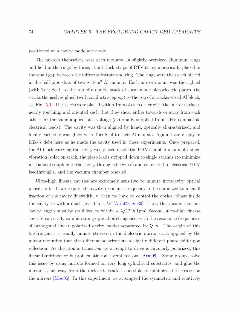
74 CHAPTER 5. THE BROADBAND CAVITY QED APPARATUS
positioned at a cavity mode anti-node.
The mirrors themselves were each mounted in slightly oversized aluminum rings
and held in the rings by three, 15mil thick strips of RTV655 symmetrically placed in
the small gap between the mirror substrate and ring. The rings were then each placed
in the half-pipe slots of two 1cm3 Al mounts. Each mirror-mount was then glued
(with Torr Seal) to the top of a double stack of shear-mode piezoelectric plates, the
stacks themselves glued (with conductive epoxy) to the top of a cracker-sized Al block,
see Fig. 5.1. The stacks were placed within 1mm of each other with the mirror surfaces
nearly touching, and oriented such that they shear either towards or away from each
other, for the same applied bias voltage (externally supplied from UHV-compatible
electrical leads). The cavity was then aligned by hand, optically characterized, and
finally each ring was glued with Torr Seal to their Al mounts. Again, I am deeply in
Mike’s debt here as he made the cavity used in these experiments. Once prepared,
the Al-block carrying the cavity was placed inside the UHV chamber on a multi-stage
vibration isolation stack, the piezo leads stripped down to single strands (to minimize
mechanical coupling to the cavity through the wires) and connected to electrical UHV
feedthroughs, and the vacuum chamber resealed.
Ultra-high finesse cavities are extremely sensitive to minute intracavity optical
phase shifts. If we require the cavity resonance frequency to be stabilized to a small
fraction of the cavity linewidth, κ, then we have to control the optical phase inside
the cavity to within much less than πF [Arm09, Sie86]. First, this means that our
cavity length must be stabilized to within ! λ2F 1pm! Second, ultra-high finesse
cavities can easily exhibit strong optical birefringence, with the resonance frequencies
of orthogonal linear polarized cavity modes separated by Á κ. The origin of this
birefringence is usually minute stresses in the dielectric mirror stack applied by the
mirror mounting that give different polarizations a slightly different phase shift upon
reflection. As the atomic transition we attempt to drive is circularly polarized, this
linear birefringence is problematic for several reasons [Arm09]. Some groups solve
this issue by using mirrors formed on very long cylindrical substrates, and glue the
mirror as far away from the dielectric stack as possible to minimize the stresses on
the mirrors [Moo05]. In this experiment we attempted the symmetric and relatively

5.2. THE CAVITY 75
−0.02 −0.015 −0.01 −0.005 0 0.005 0.01 0.015 0.02 0.025
0.4
0.5
0.6
0.7
0.8
0.9
1
Time [s]
Fra
ctio
nal t
rans
mis
sion
Cavity Transmission at κ detuning
0 500 1000 1500 2000 2500 3000 3500 4000 4500 50000
1
2
3
4
5
6
7
8
9x 10
5
Frequency [Hz]
Pow
er [a
rb. u
nits
]
Transmission Power Spectrum
Figure 5.2: Using only a 300V battery to tune the empty cavity resonance κ fromthe optical probe frequency, and despite passive stabilization, cavity instability issignificant even on kHz timescales. The transmitted power was measured with directdetection (top). Bottom plot shows the power spectrum of the transmission signal,with instability noise out to 2kHz.
weak mounting with the RTV strips.
This solution yielded a cavity with no perceptible birefringence, but unfortunately
had far greater mechanical stability issues than the previous cQED experiment. The
finesse of the cavity used in this work is more than twice that of the first cavity (F 130, 000) [Arm09, AMM09], meaning the stability constraints are also more than twice
as stringent. The relative floppiness of the RTV mounting probably also contributed
to the instability issues. For example, using only a battery voltage to supply the
piezo bias to define the mirror separation and the cavity resonance κ-detuned from
the the optical probe, the cavity-transmitted power is seen to fluctuate by almost
50% on ms-timescales, Fig. 5.2. We are still unsure of the origin of this instability
noise, but it is suspected to be mechanical vibrations in the piezo stack wires ‘short
circuiting’ the vibration isolation stack [Arm09], despite efforts to mechanically de-
couple these wires from the cavity mount. Efforts to actively compensate for these

76 CHAPTER 5. THE BROADBAND CAVITY QED APPARATUS
(a) (b)
102
103
104
105
−20
0
20
40
60
|(er
ror)
/(in
put)
|2 (dB
)
Cavity stabilization transfer function
102
103
104
105
−200
−100
0
100
200
Hz
arg[
(err
or)/
(inpu
t)] (
deg)
Figure 5.3: (a), Mechanical resonances in the Al block on which the cavity wasmounted, measured by microphone and tapping the bare, suspended block. Thelargest resonances appeared to be near-fundamental flexure modes, with an antinoderight where the cavity was placed. (b), Electro-optical Bode plot of the cavity as seenby its stabilization circuit. With the cavity length stabilized with only a 100Hzbandwidth servo, the AC piezo voltage to PDH error signal was mapped out, withapparent resonances corresponding to the modes of the Al block.
mechanical fluctuations using the standard Pound-Drever-Hall (PDH) cavity locking
technique [DHK83] were hindered by 5, 10, 12kHz and mechanical resonances in the
Al block, see Fig. 5.3a, which appeared to be near-fundamental, drumhead flexure
modes. Although eventually minimized with strategically placed (mechanically lossy)
Viton tabs and a complex PID controller, these cavity instabilities were a constant
technical difficulty; the cavity construction design could still be improved.
5.3 A tour of the apparatus
5.3.1 Science cavity locking and probing
Again, the apparatus used in this experiment was inherited from our group’s earlier
cQED work [Arm09, AMM09], and largely constructed by Mike Armen and Tony
Miller. Although significant structural re-arrangement of the optics, overhauls of
many supporting electronics, and more sophisticated modulation of the cavity probes
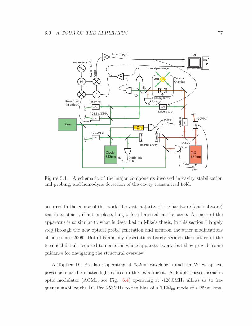
5.3. A TOUR OF THE APPARATUS 77
0
90
AOM1
AOM2
AOM3
AO
M4
Drive E, Δ, φ
Cav
ity
Θ
Vacuum
Chamber
Homodyne Fringe
Am
plit
ud
e
Qu
ad
.
Phase Quad.
(fringe lock)
Heterodyne LO
Transfer CavityTi:S lock
to TC
Slow
Fast
Diode lock
to TC
TC lock
to Cs ref.
Science cavity
lock
DAQ
Sig
LO
EOM1
Diode
852nmTi:S
832nm
Cs
Event Trigger
EO
M2
Slave
-253MHz
(126.5-Δ/2)MHz
-126.5MHz
~90MHz
MOT
Figure 5.4: A schematic of the major components involved in cavity stabilizationand probing, and homodyne detection of the cavity-transmitted field.
occurred in the course of this work, the vast majority of the hardware (and software)
was in existence, if not in place, long before I arrived on the scene. As most of the
apparatus is so similar to what is described in Mike’s thesis, in this section I largely
step through the new optical probe generation and mention the other modifications
of note since 2009. Both his and my descriptions barely scratch the surface of the
technical details required to make the whole apparatus work, but they provide some
guidance for navigating the structural overview.
A Toptica DL Pro laser operating at 852nm wavelength and 70mW cw optical
power acts as the master light source in this experiment. A double-passed acoustic
optic modulator (AOM1, see Fig. 5.4) operating at -126.5MHz allows us to fre-
quency stabilize the DL Pro 253MHz to the blue of a TEM00 mode of a 25cm long,

78 CHAPTER 5. THE BROADBAND CAVITY QED APPARATUS
mechanically-stable ‘transfer cavity’ (TC) using the PDH method and a servo band-
width of 500kHz. A small fraction of the DL Pro’s output power is also used in a
Cs modulation transfer spectrometer to measure the laser’s frequency deviation from
the p6S12, F 4q Ø p6P32, F 5q atomic transition, producing an error signal that
is servo’ed at 100Hz to lock the transfer cavity resonance to this atomic reference.
The primary purpose of the transfer cavity is to provide a stable frequency refer-
ence for the ‘science’ 852nm lasers and a ‘science cavity locking’ laser system operating
at 832nm. The 832nm laser is sourced from a titanium-sapphire (Ti:S) monolithic
block resonator that is also frequency locked to the transfer cavity via PDH, with
feedback to the Ti:S etalon and a double passed AOM (operating at 90MHz). As
the transfer cavity is 25cm long, FSR 797MHz, the available resonant modes
are far denser in frequency than in the 27µm-long science cavity. Despite this, it
is impossible to pick a TC configuration such that the TC-locked DL Pro and Ti:S
lasers are also co-resonant with the science cavity. A Photline waveguide electro-
optic modulator (EOM2) is used to put broadband-tunable frequency sidebands on
the Ti:S carrier frequency that provide the needed additional degree of freedom. One
of these sidebands serves as the ‘laser’ for a transmission-PDH lock of the science cav-
ity length. While the Ti:S carrier is ultimately referenced to the Cs line via the TC,
EOM2 can produce an optical frequency exactly two science cavity FSR away from
the desired 852nm resonance frequency (thus setting the probe-cavity detuning Θ
in the experiment).
The secondary purpose of the transfer cavity is to spectrally ‘scrub’ the 852nm
laser. As our measurements rely on sensitive optical homodyne measurements, and
the science cavity effectively adds several meters of delay in one of the arms of the
‘interferometer,’ laser phase noise was significantly above the local oscillator shot noise
in the critical 1-10MHz band of our measurements for large science-cavity drive powers
(several nW). The solution to this difficulty was to use the dramatically narrower
852nm laser transmitted by the 8kHz-linewidth TC as the optical reference in the
experiment, see Fig. 5.5. As only a few µW were transmitted by the narrow-line TC,
it is used to seed a homemade slave diode laser. Remarkably, the narrow line of the
TC-transmitted DL Pro laser was perfectly replicated by the 100mW slave laser,
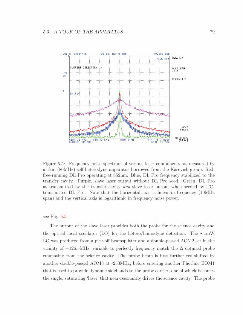
5.3. A TOUR OF THE APPARATUS 79
Figure 5.5: Frequency noise spectrum of various laser components, as measured bya 1km (80MHz) self-heterodyne apparatus borrowed from the Kasevich group. Red,free-running DL Pro operating at 852nm. Blue, DL Pro frequency stabilized to thetransfer cavity. Purple, slave laser output without DL Pro seed. Green, DL Proas transmitted by the transfer cavity and slave laser output when seeded by TC-transmitted DL Pro. Note that the horizontal axis is linear in frequency (10MHzspan) and the vertical axis is logarithmic in frequency noise power.
see Fig. 5.5.
The output of the slave laser provides both the probe for the science cavity and
the optical local oscillator (LO) for the hetero/homodyne detection. The 1mW
LO was produced from a pick-off beamsplitter and a double-passed AOM2 set in the
vicinity of +126.5MHz, variable to perfectly frequency match the ∆ detuned probe
emanating from the science cavity. The probe beam is first further red-shifted by
another double-passed AOM3 at -253MHz, before entering another Photline EOM1
that is used to provide dynamic sidebands to the probe carrier, one of which becomes
the single, saturating ‘laser’ that near-resonantly drives the science cavity. The probe
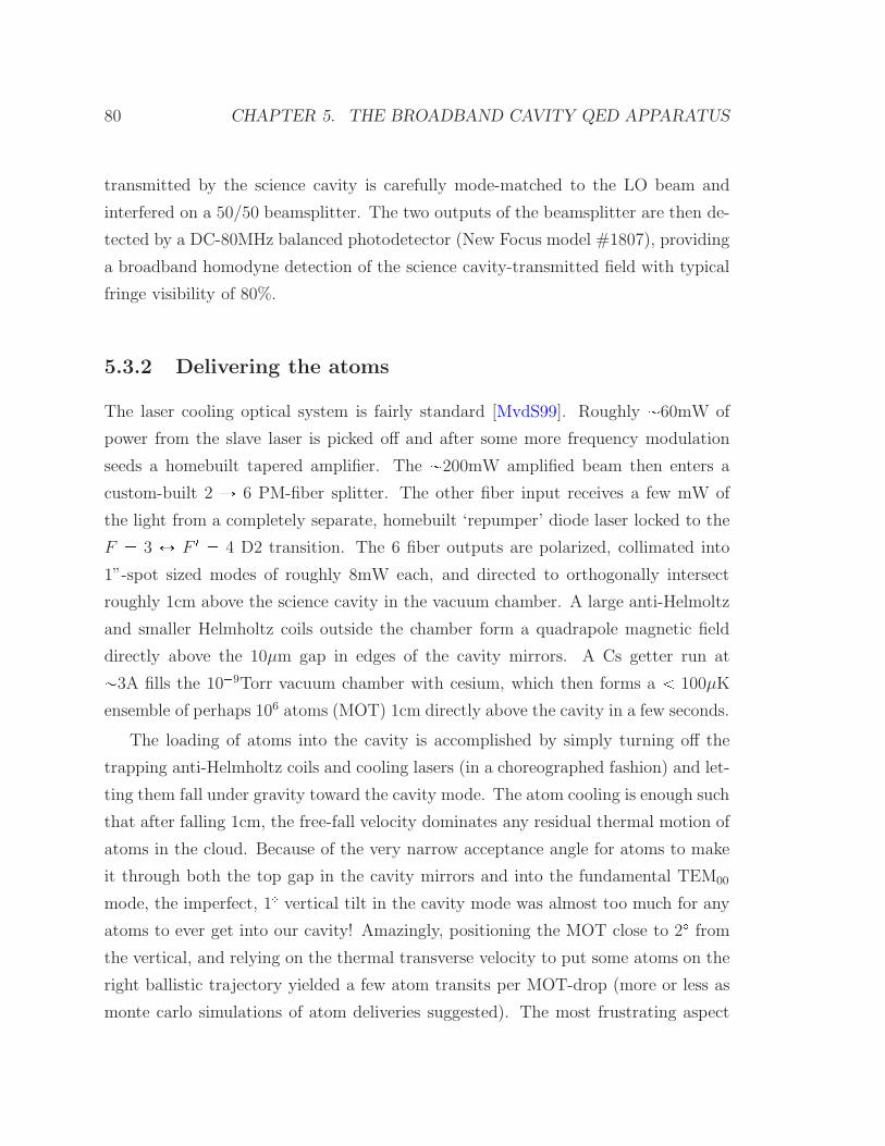
80 CHAPTER 5. THE BROADBAND CAVITY QED APPARATUS
transmitted by the science cavity is carefully mode-matched to the LO beam and
interfered on a 50/50 beamsplitter. The two outputs of the beamsplitter are then de-
tected by a DC-80MHz balanced photodetector (New Focus model #1807), providing
a broadband homodyne detection of the science cavity-transmitted field with typical
fringe visibility of 80%.
5.3.2 Delivering the atoms
The laser cooling optical system is fairly standard [MvdS99]. Roughly 60mW of
power from the slave laser is picked off and after some more frequency modulation
seeds a homebuilt tapered amplifier. The 200mW amplified beam then enters a
custom-built 2 Ñ 6 PM-fiber splitter. The other fiber input receives a few mW of
the light from a completely separate, homebuilt ‘repumper’ diode laser locked to the
F 3 Ø F 1 4 D2 transition. The 6 fiber outputs are polarized, collimated into
1”-spot sized modes of roughly 8mW each, and directed to orthogonally intersect
roughly 1cm above the science cavity in the vacuum chamber. A large anti-Helmoltz
and smaller Helmholtz coils outside the chamber form a quadrapole magnetic field
directly above the 10µm gap in edges of the cavity mirrors. A Cs getter run at3A fills the 109Torr vacuum chamber with cesium, which then forms a 100µK
ensemble of perhaps 106 atoms (MOT) 1cm directly above the cavity in a few seconds.
The loading of atoms into the cavity is accomplished by simply turning off the
trapping anti-Helmholtz coils and cooling lasers (in a choreographed fashion) and let-
ting them fall under gravity toward the cavity mode. The atom cooling is enough such
that after falling 1cm, the free-fall velocity dominates any residual thermal motion of
atoms in the cloud. Because of the very narrow acceptance angle for atoms to make
it through both the top gap in the cavity mirrors and into the fundamental TEM00
mode, the imperfect, 1 vertical tilt in the cavity mode was almost too much for any
atoms to ever get into our cavity! Amazingly, positioning the MOT close to 2 fromthe vertical, and relying on the thermal transverse velocity to put some atoms on the
right ballistic trajectory yielded a few atom transits per MOT-drop (more or less as
monte carlo simulations of atom deliveries suggested). The most frustrating aspect

5.3. A TOUR OF THE APPARATUS 81
of the atom delivery was actually the fiber splitter. Despite taking good care of the
polarization of the injected light and thermal stabilization, the power balance in the
splitter was off by a factor of 2 in some places, and changed slowly in time. Moreover,
the polarization exiting the PM fibers was hardly stable, and it typically took a few
hours of repeated MOT-dropping for the entire splitter to thermalize to the switching
beams before the polarization (and thus MOT) stabilized to something serviceable.
Thankfully, the fiber-splitter has since been replaced with a free-space beam delivery
system.
5.3.3 Transit detection and homodyne measurements
While the entire MOT cloud takes only a few ms to pass by the cavity, each individual
atom that interacts with the cavity mode in free-fall spends only 40µs in a coupled
state. With only a few atoms near-maximally coupled per MOT-drop, it’s essential
that we trigger our experiment on maximal-coupling events.
With the science cavity locked to the appropriate resonance frequency for the
experiment, and while the MOT is loading, the probe is detuned from its experimental
frequency by a few MHz and attenuated to a power such that the cavity without any
atom has a mean intracavity intensity below the atomic saturation point. In this
non-saturation regime, the semiclassical MBE (3.17) predict that the steady state
intracavity field with an atom-position dependent coupling isxayunsat E 1pγK i∆1qpκ iΘ1qpγK i∆1q g2prq (5.2)
where tE 1,Θ1,∆1u are the cQED drive amplitude and detuning parameters for this
weak probe. Thus, for a near-resonant probe, a minimum in the cavity transmis-
sion corresponds to a near-maximally coupled atom. With the weak, detuned optical
probe, continuous heterodyne detection of the transmitted field can reveal the pres-
ence or absence of individual atoms in the cavity mode in real time with a high
signal to noise ratio. Fig. 5.6 shows four individual atom transits with near maximal
coupling (and a few with lesser coupling) from one MOT drop, measured from the
demodulated amplitude quadrature of a continuous heterodyne measurement trace.

82 CHAPTER 5. THE BROADBAND CAVITY QED APPARATUS
5.02 5.04 5.06 5.08 5.1 5.12 5.14 5.16 5.18 5.2
x 10−3
0
0.5
1
Time [s]
Het
erod
yne
Am
plitu
de (
V)
Atom Transit Close−Up
4.5 5 5.5 6 6.5 7
x 10−3
0
0.5
1
Het
erod
yne
Am
plitu
de (
V)
Individual Atom Transits
Figure 5.6: Individual atom transits during a single MOT-drop, as seen with am-plitude quadrature heterodyne detection of the field transmitted by the cavity witha weak and off-resonant probe. Near-maximally coupled atoms are signaled by thenear-extinction of the measurement signal. Top, several-ms long, real-time measure-ment record showing at least four, near-maximally coupled atom transits (and a fewless-coupled transits). Bottom, close up of the first near-maximally coupled transi-tion.
The continuous, weak heterodyne probe serves another important purpose. The
eventual homodyne detection critically depends on the relative optical phase between
the signal emanating from the cavity and the LO. However, over the several meters
of free-space propagation, the length of the LO and signal paths fluctuate by more
than an optical wavelength due to slow mechanical and thermal drifts. While the
amplitude quadrature of the heterodyne signal is used to identify atom transits, the
phase quadrature is continuously fedback to the FM-modulation input of the RF
generator that drives the LO-shifting AOM2, locking the phase-quadrature signal to

5.3. A TOUR OF THE APPARATUS 83
zero with a 1kHz unity gain bandwidth and thus also locking the relative optical
phase of the signal and LO beams. As the atom transits and the experiment itself last
for a small fraction of a ms, this slow feedback loop guarantees that the homodyne
measurement experiments may be performed with a known optical phase-reference.
Rather than record the atom transits, as in Fig. 5.6, the amplitude quadrature of
the demodulated heterodyne signal is fed into a fast Schmitt trigger that compares the
transmitted optical signal to a low voltage threshold deemed to signify the presence
of a maximally-coupled atom. The firing of the Schmitt trigger causes the cavity
probe to be frequency, phase, and amplitude shifted to the appropriate settings for
measuring the dynamical response of the cQED system with a saturating drive. Its
firing is also recorded by the fast, 200MS/s GageScope card used for data acquisition.
As the signal produced by the balanced photodetector is recorded over the entire
period that the MOT cloud is expected to be in the vicinity of the cavity, this signal
from the Schmitt trigger is critical to mark the point in time that the experiment
actually began. In some experiments, the experimental probe drive was amplitude
modulated at relatively fast 1MHz frequencies, achieved by driving EOM1 with the
AM-modulated RF signal. Giving an RF signal such fast AM was a bit tricky. First,
a fixed amplitude RF-signal at the desired carrier frequency was sent to the L-port
of a standard RF mixer. Using an arbitrary function generator (also triggered by
the Schmitt) to drive the I-port, the envelope of the RF signal was modulated on
the R-port output, essentially driving the mixer “backwards.” In experiments that
required two laser drives within 1GHz of the cQED resonances, two RF generators
drove EOM1 separably, producing four optical sidebands on the probe beam, of which
two served as the coherent drives in the experiment.
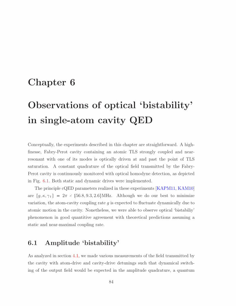
Chapter 6
Observations of optical ‘bistability’
in single-atom cavity QED
Conceptually, the experiments described in this chapter are straightforward. A high-
finesse, Fabry-Perot cavity containing an atomic TLS strongly coupled and near-
resonant with one of its modes is optically driven at and past the point of TLS
saturation. A constant quadrature of the optical field transmitted by the Fabry-
Perot cavity is continuously monitored with optical homodyne detection, as depicted
in Fig. 6.1. Both static and dynamic drives were implemented.
The principle cQED parameters realized in these experiments [KAPM11, KAM10]
are tg, κ, γKu 2π t56.8, 9.3, 2.6uMHz. Although we do our best to minimize
variation, the atom-cavity coupling rate g is expected to fluctuate dynamically due to
atomic motion in the cavity. Nonetheless, we were able to observe optical ‘bistabiliy’
phenomenon in good quantitive agreement with theoretical predictions assuming a
static and near-maximal coupling rate.
6.1 Amplitude ‘bistability’
As analyzed in section 4.1, we made various measurements of the field transmitted by
the cavity with atom-drive and cavity-drive detunings such that dynamical switch-
ing of the output field would be expected in the amplitude quadrature, a quantum
84
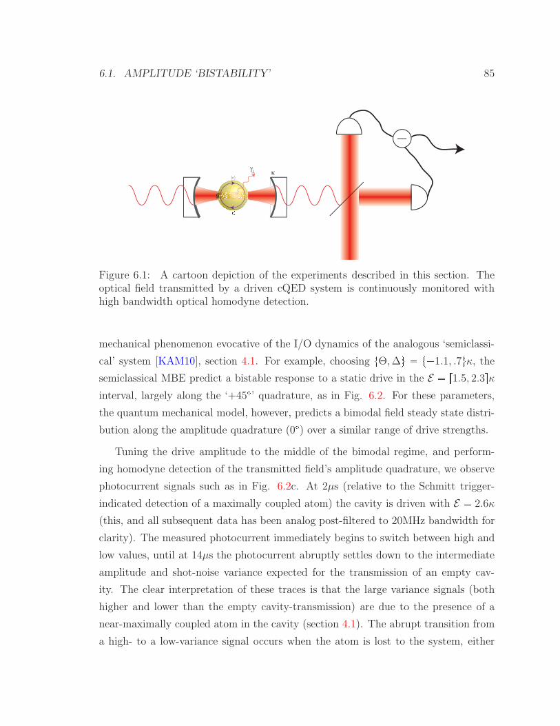
6.1. AMPLITUDE ‘BISTABILITY’ 85
κγ⊥
g
Figure 6.1: A cartoon depiction of the experiments described in this section. Theoptical field transmitted by a driven cQED system is continuously monitored withhigh bandwidth optical homodyne detection.
mechanical phenomenon evocative of the I/O dynamics of the analogous ‘semiclassi-
cal’ system [KAM10], section 4.1. For example, choosing tΘ,∆u t1.1, .7uκ, thesemiclassical MBE predict a bistable response to a static drive in the E r1.5, 2.3sκinterval, largely along the ‘+45’ quadrature, as in Fig. 6.2. For these parameters,
the quantum mechanical model, however, predicts a bimodal field steady state distri-
bution along the amplitude quadrature (0) over a similar range of drive strengths.
Tuning the drive amplitude to the middle of the bimodal regime, and perform-
ing homodyne detection of the transmitted field’s amplitude quadrature, we observe
photocurrent signals such as in Fig. 6.2c. At 2µs (relative to the Schmitt trigger-
indicated detection of a maximally coupled atom) the cavity is driven with E 2.6κ
(this, and all subsequent data has been analog post-filtered to 20MHz bandwidth for
clarity). The measured photocurrent immediately begins to switch between high and
low values, until at 14µs the photocurrent abruptly settles down to the intermediate
amplitude and shot-noise variance expected for the transmission of an empty cav-
ity. The clear interpretation of these traces is that the large variance signals (both
higher and lower than the empty cavity-transmission) are due to the presence of a
near-maximally coupled atom in the cavity (section 4.1). The abrupt transition from
a high- to a low-variance signal occurs when the atom is lost to the system, either

86 CHAPTER 6. OBSERVATIONS OF OPTICAL ‘BISTABILITY’
0.5 1 1.50.51
1.5
0
1
2
3
Mean−field steady state α vs. variable drive
Re(α)Im(α)
E [
κ]
stable solutionunstable solution
0 5 10 15 20
0
1
2
3
Amplitude quadrature photocurrent
Time [μ s]
Ph
oto
curr
en
t [α
]
drive triggered atom lost
(a) (b) (c)
Figure 6.2: (from [KAM10]) (a), Steady-state intracavity field amplitude α fromthe MBE as a function of the cavity drive amplitude E for the experimental systemwith tΘ,∆u t1.1, .7uκ. The dynamical stability of the steady-state solutions isdepicted in red and blue. (b), Wigner functions of the steady-state cavity field fromthe quantum model as a function of drive amplitude for the same parameters as (a).(c), Sample trace of amplitude quadrature homodyne measurement of the transmittedfield during an atom transit, as described in the text, with the drive turned on att 2µs and held at E 2.6κ.
because of pumping into the Cs F 3 ‘dark’ ground state or the atom exiting the
cavity. In fact, in this representative trace, the switching variance appears to slowly
decrease from a maximal value at 2µs before the abrupt loss at 14µs. This is consistent
with the expectation that the atom coupling is also a dynamic variable, with smaller
effective g’s typically yielding less splitting between the steady state intracavity lobes,
and thus also lower variance homodyne signals.
By taking the largest variance, few-µs sections of photocurrent signals from var-
ious experimental configurations, we can compare our data to the steady state I/O re-
sponse predicted by the quantum mechanical model. With tΘ,∆, Eu t1.1, .7, 2.6uκ(using the 20MHz bandwidth and calibrated detection efficiency that would vary from
10% to 20% – due to free-space mode-matching drifts in the homodyne detector), a
Wigner-function representation of the cavity-transmitted field appears as a amplitude-
quadrature (θ 0) bimodal distribution in Fig. 6.3a (section 2.1.3). Thus, for this cw
drive, steady state amplitude quadrature homodyne photocurrents should be sampled
from a bimodal distribution and phase quadrature (θ π2) measurements should
be sampled from a normal distribution, as in Fig. 6.3d. The distribution of accu-
mulated, maximum variance photocurrent data from both quadrature measurements

6.1. AMPLITUDE ‘BISTABILITY’ 87
Figure 6.3: (from [KAM10]) (a-c), Wigner function representations of the expectedsteady state photocurrent distributions, using calibrated detection efficiencies andbandwidths, for three sets of detuning and drive parameters. (d-f), Histograms rep-resenting the phase- (απ2) and amplitude-quadrature (α0) photocurrent distributionsfrom ensembles of the highest-variance segments, for the same drive parameters. Thehistograms are compared with theoretically expected distributions obtained from cor-responding Wigner functions (a-c), respectively.
matches the expected distributions calculated from the Wigner representation. Ex-
ploring other parameter ranges, further detuning the probe from the atom such thattΘ,∆, Eu t1, 3, 2.6uκ, rather than an equal-bimodal distribution, the steady state
population is expected to be biased toward the low-amplitude state, as the drive
threshold for atomic saturation increases with |∆|. Again, measurements of both
quadratures correspond well with the predicted marginal distributions in Fig. 6.3e.
Finally, increasing the drive into the saturation regime to tΘ,∆, Eu t1, 3, 3.7uκ,an even, bimodal distribution in the amplitude quadrature is both expected and
observed in Fig. 6.3f. All the data in Fig. 6.3 are in agreement with quantum the-
oretical predictions despite the use of a somewhat idealized model that assumes a
static coupling rate g (whereas g actually depends upon atomic position and Zeeman

88 CHAPTER 6. OBSERVATIONS OF OPTICAL ‘BISTABILITY’
10−2
10−1
100
1010.5
0.75
1Amplitude quadrature photocurrent autocorrelation
Time [µ s]
Aut
ocor
rela
tion
[nor
mal
ized
]
experimentsimulationno atom
κ−1
Figure 6.4: (from [KAM10]) The autocorrelation function for the same amplitudequadrature photocurrent data presented as a histogram in Fig. 6.3d is displayedin black. Blue crosses represent the autocorrelation of photocurrents simulated byquantum trajectory methods for identical parameters. The autocorrelation of thesequasi-bistable signals is enhanced relative to normalized experimental empty cavitytransmission data (red pluses), also presented here with a 20MHz analog bandwidth,and the κ1 17ns cavity decay time (dashed orange line).
sub-state, and can vary within a photocurrent segment because of atomic motion
and optical pumping). Although it may be possible to apply quantum smoothing
techniques [Tsa09] to estimate time-varying atomic coupling trajectories on a shot-
by-shot basis from the data, I used a simple fixed effective value g .8 g0 in the
analysis for all three parameter sets (the only fit in Fig. 6.3). Quantum trajectory
simulations further suggest that this approximation of fixed g and the finite (20 MHz)
bandwidth of the presented homodyne signals account for slight mismatches between
theory and experiment in the amplitude quadrature splitting and phase-quadrature
mean in the three data sets.
As predicted in section 4.1, even in the single-atom, 10 photon regime, dis-
tinct high- and low-amplitude states of the output field are expected. Signatures
of this remnant optical bistability are visible in the bimodal output photocurrents of
Fig. 6.3. Similarly, we see from the same data in Fig. 6.4 that although the output field
switches spontaneously when an atom is present in the cavity, it remains correlated
over timescales much longer than that of light transmitted through an empty cavity.
This atom-induced memory effect can be seen as a quantum remnant of semiclassical
optical bistability, where classically the high- and low-amplitude states are truly sta-
ble (due to negligible fluctuations in the system) and would therefore exhibit infinite

6.1. AMPLITUDE ‘BISTABILITY’ 89
15 20 25
0
2
4
Time [μ s]
Pho
tocu
rren
t [α
]
15 20 25
0
2
4
Photocurrent @ .25MHz AM
E [κ
]
12 14 16 18 20
0
2
4
Pho
tocu
rren
t [α
] Photocurrent @ 1MHz AM
12 14 16 18 20
0
2
4
Time [μ s]
E [κ
]
(a) (b)
(c) (d)
E [κ] E [κ]
Figure 6.5: (from [KAM10]) (a-b), Single-shot, amplitude quadrature measurementsas the drive amplitude is swept at .25MHz and 1MHz, respectively. Black traces are20MHz bandwidth photocurrents while the green, dashed traces represent the instan-taneous drive amplitude. (c-d), dashed red (blue) traces portray the same photocur-rent data in (a) and (b), respectively, as a function of the instantaneous increasing(decreasing) drive amplitude. Error bars represent sample mean and variance of thesame photocurrents within non-overlapping drive amplitude intervals. Red and blueregions represent theoretically expected photocurrent mean and sample variance as afunction of instantaneous drive (section 2.1.3).
correlation time. Consequently, it should also be possible to observe the hysteretic am-
plitude response characteristic of semiclassical optical bistability by modulating the
system drive slowly compared to the timescale for relaxation of the intracavity field
(set in our case by the cavity decay time) but rapidly compared to the ‘metastable’
memory timescale indicated in Fig. 6.4. Accordingly, the data in Fig. 6.5 were ob-
tained by recording amplitude-quadrature homodyne photocurrents while sweeping
the drive strength sinusoidally at 0.25MHz or 1MHz. Figs. 6.5a and 6.5b depict
representative single-shot photocurrent segments with tΘ,∆u t1.1, .7uκ encom-
passing several cycles of sinusoidal drive amplitude modulation (AM) spanning the
steady state bimodal region. Increases in both the mean and variance of the output

90 CHAPTER 6. OBSERVATIONS OF OPTICAL ‘BISTABILITY’
photocurrent, largely in phase with the drive amplitude, can be discerned in both of
these real-time plots. However, plotting the photocurrent as a function of the instan-
taneous drive amplitude (Figs. 6.5c and 6.5d) reveals a significant hysteresis in the
system response at 1MHz AM that is barely noticeable at the more adiabatic .25MHz
AM rate. Whereas the response of the empty cavity is linear and non-hysteretic
with fixed (shot-noise) output photocurrent variance at these modulation frequen-
cies, nonlinear increases in the signal mean and variance are evident in both traces
at mid-sweep. At 1MHz AM, a hysteresis loop appears to open between the upward
and downward drive amplitude sweeps, with the low (high) state persisting over a
wider range of increasing (decreasing) drive amplitudes than at .25MHz AM. These
data are in agreement with theoretical predictions again assuming a fixed value of
g .8 g0. It can also be shown that the slight elevation of the experimental high-
amplitude branch in Fig. 6.5d is also consistent with slight fluctuation in g over the
entire sequence, as in Fig. 6.3d.
6.2 Phase ‘bistability’
If we drive the cQED system harder and on-resonance [KAPM11], we move into a
different I/O response regime, physically distinct from the absorptive ‘bistability’
behavior. As described in section 4.2.2, in the strong-driving limit, the atom becomes
fully saturated and is forced to choose a dipole orientation either in- or completely-out
of phase with the laser drive. The orientation of the dipole determines the phase of
the field the atom re-radiates into the cavity, either 90 out of phase with the drive
(i.e. in phase with the ‘velocity’ of the electric dipole).
Rather than drive the cQED system completely on resonance, we found that sig-
nificantly improved data could be obtained by tuning both the drive and the cavity
resonance slightly to the red of the atomic transition (i.e. Θ 0, ∆ κ ¡ 0).
We attribute this signal enhancement to an attractive optical dipole force that tends
to draw the atom towards the maximally-coupled cavity anti-node positions. Luck-
ily, this opto-mechanical effect on the atom is apparently significant for ∆ κ, but
the population distribution of the low- and high-phase states is barely perturbed,

6.2. PHASE ‘BISTABILITY’ 91
Figure 6.6: Phase quadrature perspective of the steady state intracavity field Wignerfunction for the drive parameters tΘ,∆, Eu t0, 0, 3.7uκ (Left) and tΘ,∆, Eu t0, 1, 3.7uκ (Right).
so that the I/O response is nearly identical to the on-resonance case, see Fig. 6.6.
Taking the parameters tΘ,∆, Eu t0, 1, 3.7uκ, the phase quadrature photocurrent
measured during an atom transit show clear, binary switching between positive and
negative phase-shifted states in Fig. 6.7. The photocurrent segment (again, recorded
at 200MS/s but displayed with 20MHz bandwidth for clarity) resembles a random
telegraph with added Gaussian noise, featuring sporadic jumps between levels indi-
cating positive and negative phase shifts of the transmitted optical beam. Such sig-
nals stand as a marked improvement over our previous observations of TLS-induced
phase noise (as opposed to clear, binary phase switching) in Mike Armen’s thesis
work [Arm09], and more convincingly support long-standing theoretical predictions
[AC91] summarized in section 4.2.2. For example, the photocurrent histogram in
Fig. 6.7b suggests a dual-Gaussian distribution in this single shot segment, whereas
only “flat-top” distributions were previously visible after averaging many single-shot
signals in [AMM09]. Although a complex physical model is required to describe the
TLS-cavity system (section 3.2), the output of a device that possibly could function
as a random binary phase modulator should also be well described by a two-state,
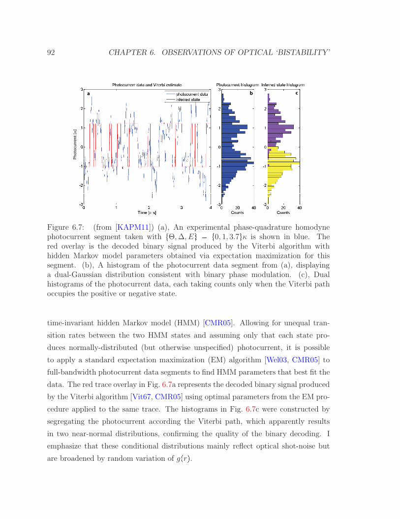
92 CHAPTER 6. OBSERVATIONS OF OPTICAL ‘BISTABILITY’
a b c
Ph
oto
curr
en
t [α
]
Figure 6.7: (from [KAPM11]) (a), An experimental phase-quadrature homodynephotocurrent segment taken with tΘ,∆, Eu t0, 1, 3.7uκ is shown in blue. Thered overlay is the decoded binary signal produced by the Viterbi algorithm withhidden Markov model parameters obtained via expectation maximization for thissegment. (b), A histogram of the photocurrent data segment from (a), displayinga dual-Gaussian distribution consistent with binary phase modulation. (c), Dualhistograms of the photocurrent data, each taking counts only when the Viterbi pathoccupies the positive or negative state.
time-invariant hidden Markov model (HMM) [CMR05]. Allowing for unequal tran-
sition rates between the two HMM states and assuming only that each state pro-
duces normally-distributed (but otherwise unspecified) photocurrent, it is possible
to apply a standard expectation maximization (EM) algorithm [Wel03, CMR05] to
full-bandwidth photocurrent data segments to find HMM parameters that best fit the
data. The red trace overlay in Fig. 6.7a represents the decoded binary signal produced
by the Viterbi algorithm [Vit67, CMR05] using optimal parameters from the EM pro-
cedure applied to the same trace. The histograms in Fig. 6.7c were constructed by
segregating the photocurrent according the Viterbi path, which apparently results
in two near-normal distributions, confirming the quality of the binary decoding. I
emphasize that these conditional distributions mainly reflect optical shot-noise but
are broadened by random variation of gprq.

6.2. PHASE ‘BISTABILITY’ 93
0 0.5 1 1.5 20
0.2
0.4
0.6
0.8
1
1.2
1.4
1.6
1.8
2
High → low [γ⊥ /2]
Low
→ h
igh
[γ⊥/2
]
Transition rates estimate for `near-detuned’ system
0 0.5 1 1.5 20
0.2
0.4
0.6
0.8
1
1.2
1.4
1.6
1.8
2
High → low [γ⊥ /2]
Low
→ h
igh
[γ⊥/2
]
Transition rates estimate for `far-detuned’ system
γ⊥ /2
T = 175 ⋅ 2/γ⊥
>Lmax
/3 indiv. region
>Lmax
/3 overall region
>Lmax
/3 simulated region
a b
Figure 6.8: (from [KAPM11]) Both plots depict contours of the likelihood functionsof hidden Markov model transition rates for lowØhigh switching. The most likelyrate-pairs inferred from data taken from individual atom transit segments are indi-cated by grey dots, with the diameter of each dot representing the duration of thecorresponding data segment. The grey bars represent the intervals over which thelikelihood of the individual transits’ rate-pairs are at least 1/3 of their maximum.The red cross locates the most likely rate-pair, given an aggregated segment formedfrom the individual transit measurements, with the red oval enclosing the region ofrate-pair likelihoods that are at least 1/3 of the maximum. The teal cross and ovalrepresent the same likelihood contours produced from simulated data. (a), Likelihoodcontours for tΘ,∆, Eu t0, 1, 3.7uκ. (b), tΘ,∆, Eu t0, 3, 3.7uκ.
With the good visibility of the switching states, we can also confirm that binary
decoding of the experimental photocurrent segments yields transition rate estimates
that match predictions of the full quantum model (section 3.2). The plots in Fig. 6.8
depict contours of the likelihood functions of HMM parameters estimated from indi-
vidual and aggregated atom transits, obtained under two different input conditions.
Fig. 6.8a reflects data acquired from a ‘near-detuned’ system with the same param-
eters as in Fig. 6.7. The high likelihood of a symmetric switching model apparent
here is both theoretically predicted (section 4.2.2) and consistent with the symmetric
photocurrent histograms in Fig. 6.7. The slightly greater than γK2 switching rates
of the most likely models (as opposed to exactly γK2, which occurs in the strong-
driving limit) is due to the moderate power of the probe. Fig. 6.8b reflects data taken
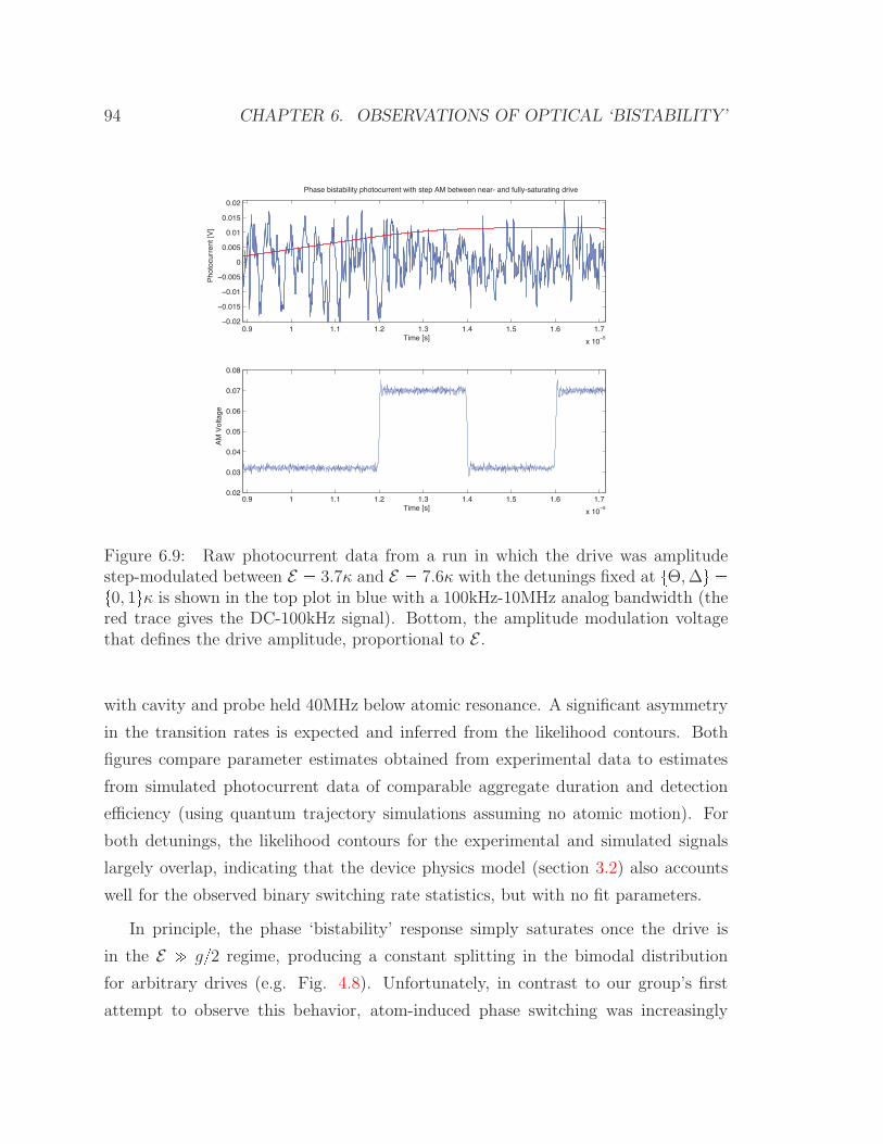
94 CHAPTER 6. OBSERVATIONS OF OPTICAL ‘BISTABILITY’
0.9 1 1.1 1.2 1.3 1.4 1.5 1.6 1.7
x 10−5
−0.02
−0.015
−0.01
−0.005
0
0.005
0.01
0.015
0.02
Phase bistability photocurrent with step AM between near- and fully-saturating drive
Time [s]
Ph
oto
curr
en
t [V
]
0.9 1 1.1 1.2 1.3 1.4 1.5 1.6 1.7
x 10−5
0.02
0.03
0.04
0.05
0.06
0.07
0.08
Time [s]
AM
Vo
ltag
e
Figure 6.9: Raw photocurrent data from a run in which the drive was amplitudestep-modulated between E 3.7κ and E 7.6κ with the detunings fixed at tΘ,∆u t0, 1uκ is shown in the top plot in blue with a 100kHz-10MHz analog bandwidth (thered trace gives the DC-100kHz signal). Bottom, the amplitude modulation voltagethat defines the drive amplitude, proportional to E .
with cavity and probe held 40MHz below atomic resonance. A significant asymmetry
in the transition rates is expected and inferred from the likelihood contours. Both
figures compare parameter estimates obtained from experimental data to estimates
from simulated photocurrent data of comparable aggregate duration and detection
efficiency (using quantum trajectory simulations assuming no atomic motion). For
both detunings, the likelihood contours for the experimental and simulated signals
largely overlap, indicating that the device physics model (section 3.2) also accounts
well for the observed binary switching rate statistics, but with no fit parameters.
In principle, the phase ‘bistability’ response simply saturates once the drive is
in the E " g2 regime, producing a constant splitting in the bimodal distribution
for arbitrary drives (e.g. Fig. 4.8). Unfortunately, in contrast to our group’s first
attempt to observe this behavior, atom-induced phase switching was increasingly

6.2. PHASE ‘BISTABILITY’ 95
rare to see, per atom transit event for drives E ¡ .8g 5κ. In contrast to drive
amplitudes below this regime (e.g. for E .6g 3.7κ), where phase bistability
effects were observed for several to tens of µs, in a majority of atom triggering events
in the very high saturation regime, phase bistable effects were rarely seen, and if
seen, only persisted for a few µs. We attribute this lack of high-drive data to the
strong drive mechanically expelling the atoms from the cavity mode with dipole force
effects. The significantly larger atom-cavity coupling in this experiment, g 2π 56.8MHz, compared to the earlier iteration, g 2π 16MHz [Arm09, AMM09],
means that the same opto-mechanical forces 9∇gprq?n present in this experiment
occurred at 13 times greater intracavity photons in the previous experiment. As
the quality of the phase bistability data in that experiment began to peter out at
about n 110, with shorter and shorter visible phase noise segments [Arm09], the
limitations of both systems seem compatible (note too, that the the earlier iteration
was also likely effected by faster dark state-pumping due to large cavity birefringence).
Importantly, amplitude step-modulating the drive strength between near- and far-
saturating regimes, we see that the high drive state causes the atom-induced phase
bistability to be lost, as in Fig. 6.9, rather than phase-bistable effects simply not
existing for very large drives. As the drive amplitude is step-modulated between
n 14 and n 58, phase switching is apparent for the initial, low-drive state, but
abruptly disappears when the drive is increased, and does not reappear when the
drive is switched low again.
Finally, despite our atomic system’s large gκ ratio, which is unfavorable for the
control method simulated in Fig. 4.9, we attempted exert an external, optical control
of the switching rate experimentally using the ‘near-detuned’ system. Fig. 6.10 shows
inferred ‘total’ transition rates (the mean rate at which switching in either direction
occurs) as a function of the power of the control beam, for three different control
beam frequencies. In the strong driving limit the optimum control detuning would
be 425MHz, but given our moderate signal power the effective coupling energy (and
therefore optimal control detuning) should be somewhat smaller. The statistical
significance of the data displayed in Fig. 6.10 is marginal, but the data do show
consistent trends that match expectations: data taken with -375MHz and -425MHz

96 CHAPTER 6. OBSERVATIONS OF OPTICAL ‘BISTABILITY’
control detuning induce higher transition rates with higher power, with -375MHz
consistently higher, while the -525MHz detuning induced essentially no net transition
increase over the accessible range of control powers (limited by opto-mechanical effects
on the high end). Linear fits to data obtained from trajectory simulations reproduce
these general trends of the data and confirm the limited degree of control achievable
in our experimental system. We thus infer an apparent control energy requirement of
only 1fJ/edge even in our atomic implementation (with unfavorable parameters for
efficient control) of the dressed-state binary phase modulator. I’d also like to point
out that the data presented in Fig. 6.10 was the last data ever taken in our group’s
Varian-Astro era, obtained the night before the lab tear-down for the Nano move!

6.2. PHASE ‘BISTABILITY’ 97
Figure 6.10: (from [KAPM11]) Data points represent inferred ‘total γ’ for vari-ous control beam parameters. The thin lines track the most likely total γ and theconfidence intervals represent the range of γ values with at least 1/3 the maximumlikelihood. The green, blue and red data points depict the total γ as a function ofcontrol power for a control probe detuned by -375MHz, -425MHz, and -525MHz fromthe signal probe, respectively. The colored shaded regions represent linear best fitsof the corresponding confidence intervals based on a simulated data set with perfectdetection efficiency and duration several times that of the experimental data. Theapparent positive, constant bias in the experimental γ relative to simulation for con-trol powers at least equal to the probe’s is perhaps due to enhanced opto-mechanicalmotion induced by a strong control beam.

Part III
Autonomous Nanophotonic
Quantum Memories
98

Introduction
Traditional approaches to quantum information theory [NC00] are non-committal to
any particular implementation. Instead, the basic concepts are framed in terms of the
axiomatic laws of quantum mechanics. This generality is a testament to the simple
power of the ideas, and allows for an impossibly large range of experiments to get
into the game, from trapped ion-computation [Win09] to liquid state NMR [VSB01].The fundamentals of quantum information can be explained using the same abstract
formalism of quantum mechanics taught to undergraduates, and usually are [NC00].
Because of this, there is a sense that experiments simply have to ‘catch up’ with
the established theory of quantum information, that qubits, gates, and measurements
that better approximate these simple ideals simply have to be realized. While this
is no doubt true, theoretical approaches framed in the natural laws of promising
systems are also lacking. It might be inappropriate that next generation quantum
information systems with trapped ions implement the same protocols as those made
from superconducting microwave circuits. But guided by equivalent, basic models, it’s
perhaps inevitable that all breeds of quantum information hardware have so far been
driven towards equivalent demonstrations [RRH04, DCG09, CLS04, DRS10,VSB01, PMO09].
In this final part, I describe some of our efforts to develop a method for de-
signing protected quantum memories out of networks of nanophotonic components
[KNPM10, KPCM11]. Modeling these systems with a framework based on a circuit
description of quantum optics, in applying basic quantum error correcting (QEC)
concepts we are naturally led to designs that are continuous and stationary in time
99

100
Figure 6.11: An example of a traditional quantum ‘circuit’ that depicts a traditionaldiscrete time version of the 3 qubit bit-flip code described in section 7.1.1.
and operate autonomously. This approach is in contrast to the traditional descrip-
tion of quantum error correction (QEC) [Got09, NC00] involving discrete operations,
clocked execution, instantaneous measurement and external corrections. These de-
signs are communicated through circuit schematics, with each ‘block’ representing a
physical device, with its own internal dynamics, and each connection between them
representing a physical optical field (e.g. Fig. 8.3). The continuous time dynamics
of this system are constructed from these diagrams simply by describing them in the
quantum circuit formalism based on quantum stochastic differential equations (QS-
DEs) (part I). Again, we like to contrast these schematics with traditional, so-called
‘quantum circuit’ diagrams composed of blocks representing discrete operations, not
devices, and the connections between them defining a chronology, not a physical cou-
pling (e.g. Fig. 6.11) [NC00]. Our designs are much more like an electrical schematic
that represents a specific hardware construction, while the traditional schematic rep-
resentation is more like a high-level programming language.
Moreover, these all-optical network designs naturally sidestep the difficulty of
having to build a distinct, classical apparatus operating in parallel with the quan-
tum memory, constantly monitoring and maintaining it. Typically, the mechanics of
this essential half of a quantum memory system are hardly considered at all, taking
a back seat in the analysis to the qubits in which the information is stored. This
assumption of a perfect, classical overseer glosses over the inherent technological mis-
match of typically fast, nanoscale and cold quantum systems with slow, mesoscopic,
and/or hot classical ones. The extreme performance demands for quantum informa-
tion processing should motivate solutions that weigh classical and quantum resources

101
wholistically and utilize system models as close to physical mechanics as possible.
Not only do our photonic networks model both the memory and controller on equal
footing, but they do so in a technologically homogenous context.

Chapter 7
Preliminary Models
The focus of the work described in this final part has been the design of nanophotonic
networks that could form a protected quantum memory element and require a min-
imum of external maintenance. Before we can get to the full designs, though, basic
concepts of quantum error correction, and the intuition behind and continuous-time
models of the nanophotonic components need to be introduced.
7.1 Quantum error correction
Quantum error correction (QEC) addresses the problem of how to do ‘nothing’
[Got09, NC00]. Simply staying in the same state for an extended period of time
is difficult for quantum objects, especially for highly entangled, many body systems.
Uncontrolled, unmonitored interactions between a quantum state we’d like to pre-
serve and its environment generally ruin the utility of the stored state. While noise is
a problem in classical memory banks too, of course, the problem of preserving a single
qubit of quantum information is more subtle. For instance, we can’t simply copy a
state to protect it through redundancy; measuring quantum states to diagnose errors
will perturb the states in general; and errors on spin-1/2 qubits are usually contin-
uous rotations, not discrete operations [NC00]. Rather than summarize the general
theories of stabilizer QEC [Got09], I will directly explain the operation of three basic
quantum codes our networks emulate.
102
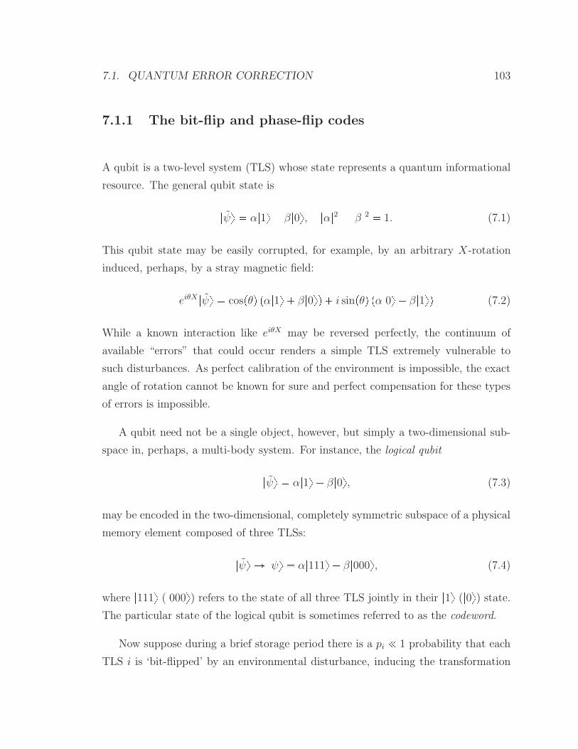
7.1. QUANTUM ERROR CORRECTION 103
7.1.1 The bit-flip and phase-flip codes
A qubit is a two-level system (TLS) whose state represents a quantum informational
resource. The general qubit state is|ψy α|1y β|0y, |α|2 |β|2 1. (7.1)
This qubit state may be easily corrupted, for example, by an arbitrary X-rotation
induced, perhaps, by a stray magnetic field:
eiθX |ψy cospθq pα|1y β|0yq i sinpθq pα|0y β|1yq (7.2)
While a known interaction like eiθX may be reversed perfectly, the continuum of
available “errors” that could occur renders a simple TLS extremely vulnerable to
such disturbances. As perfect calibration of the environment is impossible, the exact
angle of rotation cannot be known for sure and perfect compensation for these types
of errors is impossible.
A qubit need not be a single object, however, but simply a two-dimensional sub-
space in, perhaps, a multi-body system. For instance, the logical qubit|ψy α|1y β|0y, (7.3)
may be encoded in the two-dimensional, completely symmetric subspace of a physical
memory element composed of three TLSs:|ψy Ñ |ψy α|111y β|000y, (7.4)
where |111y (|000y) refers to the state of all three TLS jointly in their |1y (|0y) state.The particular state of the logical qubit is sometimes referred to as the codeword.
Now suppose during a brief storage period there is a pi ! 1 probability that each
TLS i is ‘bit-flipped’ by an environmental disturbance, inducing the transformation
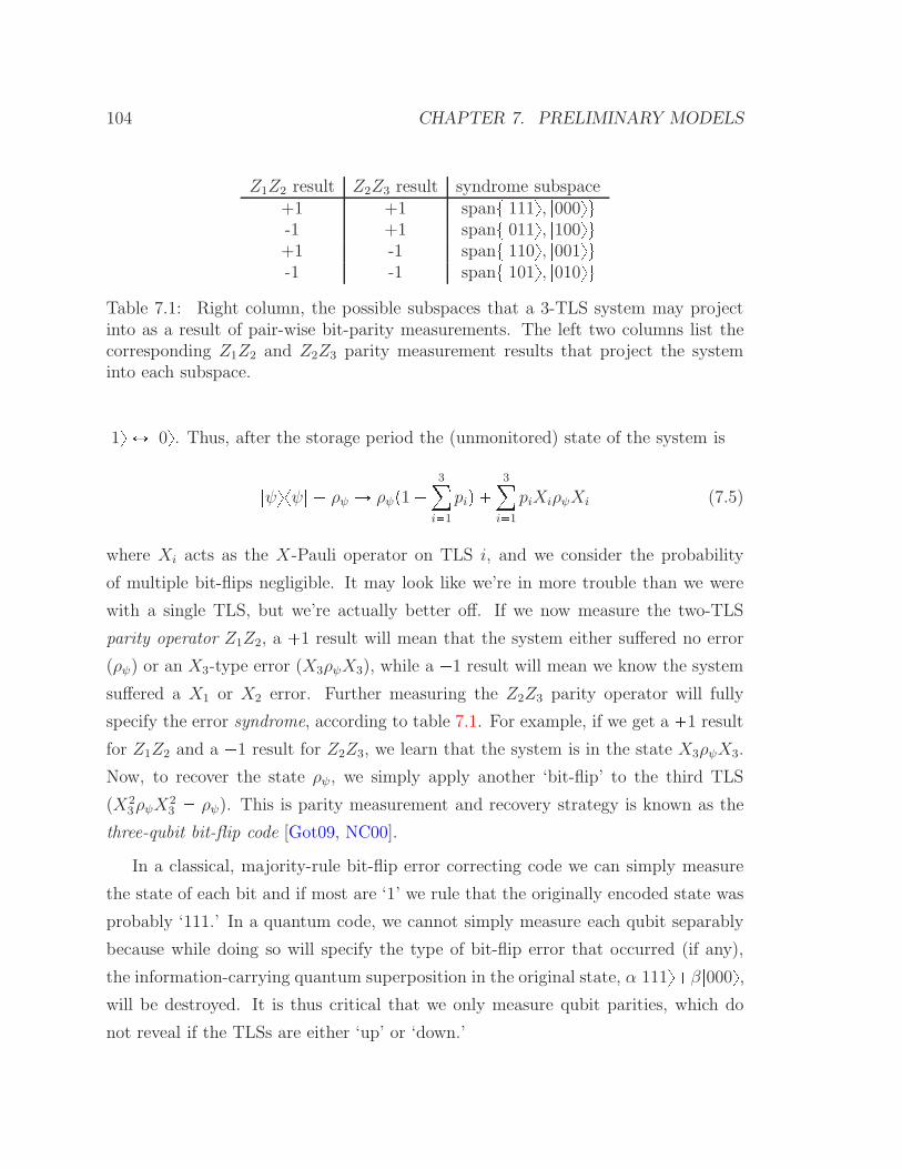
104 CHAPTER 7. PRELIMINARY MODELS
Z1Z2 result Z2Z3 result syndrome subspace+1 +1 spant|111y, |000yu-1 +1 spant|011y, |100yu+1 -1 spant|110y, |001yu-1 -1 spant|101y, |010yu
Table 7.1: Right column, the possible subspaces that a 3-TLS system may projectinto as a result of pair-wise bit-parity measurements. The left two columns list thecorresponding Z1Z2 and Z2Z3 parity measurement results that project the systeminto each subspace.|1y Ø |0y. Thus, after the storage period the (unmonitored) state of the system is|ψyxψ| ρψ Ñ ρψp1 3
i1
piq 3
i1
piXiρψXi (7.5)
where Xi acts as the X-Pauli operator on TLS i, and we consider the probability
of multiple bit-flips negligible. It may look like we’re in more trouble than we were
with a single TLS, but we’re actually better off. If we now measure the two-TLS
parity operator Z1Z2, a 1 result will mean that the system either suffered no error
(ρψ) or an X3-type error (X3ρψX3), while a 1 result will mean we know the system
suffered a X1 or X2 error. Further measuring the Z2Z3 parity operator will fully
specify the error syndrome, according to table 7.1. For example, if we get a 1 result
for Z1Z2 and a 1 result for Z2Z3, we learn that the system is in the state X3ρψX3.
Now, to recover the state ρψ, we simply apply another ‘bit-flip’ to the third TLS
(X23ρψX
23 ρψ). This is parity measurement and recovery strategy is known as the
three-qubit bit-flip code [Got09, NC00].
In a classical, majority-rule bit-flip error correcting code we can simply measure
the state of each bit and if most are ‘1’ we rule that the originally encoded state was
probably ‘111.’ In a quantum code, we cannot simply measure each qubit separably
because while doing so will specify the type of bit-flip error that occurred (if any),
the information-carrying quantum superposition in the original state, α|111yβ|000y,will be destroyed. It is thus critical that we only measure qubit parities, which do
not reveal if the TLSs are either ‘up’ or ‘down.’

7.1. QUANTUM ERROR CORRECTION 105
In the above bit-flip code example we presumed a very specific error model, either
TLS bit-flips occurred or they didn’t, which may seem a serious limitation if our errors
are more likely to be continuous rotations. However, one of the most powerful con-
cepts in QEC is that if a code can correct for the random application of error operatorstEu, then it can also correct for the random application of arbitrary linear combina-
tions of tEu [NC00]. Thus, since the bit-flip code works in the above pi ! 1 example
where tEu tI,X1, X2, X3u, it also works when tEu expriθtI,X1, X2, X3us. Thisremarkable result can be understood as a consequence of the measurement proce-
dure discretizing ‘analog’ errors. Even if a possible bit-rotation acting on TLS i is
not θ π2, measuring Z1Z2 and Z2Z3 forces the system into either |ψy or Xi|ψy.Thus, although continuous error models are appropriate in quantum information sys-
tems, QEC has more in common with digital classical error correction than (famously
impractical) analog error correction.
However, what about the finite possibility in the bit-flip example that multiple
bit-flip errors occur? In these cases, the strategy fails: if the first two TLSs flip, the
algorithm will erroneously determine that the third TLS flipped and apply the wrong
correction. Hence, the general notion is that QEC has to be done repeatedly and
rapidly enough such that the likelihood of multiple, independent single-TLS errors is
negligible. Moreover, what if the errors are of a different sort, such as Z-rotations?
Z-errors map |1y Ñ |1y and |0y Ñ |0y, and are consequently known as phase errors.
Again, the bit-flip code is helpless against such error types. However, if these are the
only type of error affecting each TLS, we can apply an analogous strategy and encode|ψy Ñ |ψy α| y β| y, (7.6)
where |y 1?2p|1y |0yq, and measure the phase-parity operators X1X2 and X2X3,
performing the analogous error decoding and recovery. This three qubit phase-flip
code is related to the bit-flip code via a simple basis change, and shares the analogous
advantages and limitations.
While very promising, both codes are also very limited, only capable of protecting
against a narrow class of errors. To make more powerful, general QEC codes, a

106 CHAPTER 7. PRELIMINARY MODELS
(a)
Q1,1 Q1,2 Q1,3
Q2,1 Q2,2 Q2,3
Q3,1 Q3,2 Q3,3
X2, X3,∗ ∗
Z ,1 Z ,2∗ ∗
Stabilizer generator examples
(b)
Q1,1 Q1,2 Q1,3
Q2,1 Q2,2 Q2,3
Q3,1 Q3,2 Q3,3
ZL
Logical operators
XL
(c)
Q1,1 Q1,2 Q1,3
Q2,1 Q2,2 Q2,3
Q3,1 Q3,2 Q3,3
ZT1
XT1
ZT2
XT2
XT3 XT4
ZT3
ZT4
Gauge operators
Figure 7.1: (a), Two of the stabilizer generators in the 9 qubit Bacon-Shor code.One stabilizer generator acts as the Z operator on all qubits in the first two columns,the other generator shown acts as X on all qubits in the last two rows (the remainingtwo stabilizer generators are not shown for clarity). (b), Logical operators that acton the 2D subsystem L in the no-error subspace: boxes again indicate Z (blue) andX (green) acting on all enclosed qubits. (c), One choice for the remaining gaugeoperators that act on the remaining, 4-qubit T subsystem in the no error subspace.
memory element composed of more TLSs is needed.
7.1.2 The 9 qubit Bacon-Shor code
Abstractly, the three-qubit codes in the previous section took the strategy of decom-
posing a multibody Hilbert space into
H L` E (7.7)
where L is a 2-dimensional ‘logical space’ in which the logical qubit is encoded. Any
states in E are deemed errorful. A generalization of this subspace-coding strategy is
a subsystem code [KLP05] in which a multibody Hilbert space is decomposed into
H pLb T q ` E (7.8)

7.1. QUANTUM ERROR CORRECTION 107
where now information is encoded in the L subsystem and any state in E is in error.
Thus, while a valid logical state has the form
ρψ pρL b ρT q ` 0 (7.9)
the state of the ‘gauge subsystem’ ρT carries no information, and may be scrambled
without consequence. This general strategy is exploited by another famous code, the
9 qubit Bacon-Shor subsystem QEC code [Bac06], which is the smallest of a class
of naturally fault-tolerant QEC codes [Got09, NC00] capable of protecting a single
logical qubit from arbitrary single-TLS errors.
In this code, 9 TLSs are arranged in a 33 grid, as in Figs. 7.1. In this configu-
ration, a non-Abelian operator group is the set of operators generated by pairs of X
operators acting on adjacent-row TLSs and pairs of Z operators acting on adjacent-
column TLSs
T xXi,jXi1,j, Zj,iZj,i1|i P Z2, j P Z3y, (7.10)
where Xi,j and Zi,j act as Pauli operators on the TLS in row i, column j and as the
identity on all others. An Abelian subgroup S T known as the ‘stabilizer’ group is
generated by X operators acting on all TLSs in two adjacent rows and Z operators
acting on all TLSs in two adjacent columns
S xXi,Xi1,, Z,iZ,i1|i P Z2y, (7.11)
as depicted in Fig. 7.1a. These generators of the stabilizer group play the same role as
the parity operators Z1Z2 and Z2Z3 in the three qubit bit-flip code: measuring them
reveals which errors have occurred to the 9 TLS system. That is, the 1 eigenvalues
of the generators of S may be used to label subspaces of the H pC2qb9system
Hilbert space
H à~a
H~a, (7.12)
where ~a is a string of the four binary eigenvalues of the stabilizer generators and
each H~a represents a 25-dimensional space. Each H~a may be further decomposed into
108 CHAPTER 7. PRELIMINARY MODELS
subsystems
H~a HL~a bHT
~a (7.13)
where elements from T (which commute with S) act non-trivially on some HT~a , and as
the identity onHL~a , encoding four ‘gauge’ qubits, modulo S. This action leaves theHL
~a
as single-qubit subsystems, in one of which our logical qubit is stored. We can choose
this logical qubit to be the one encoded by the operators XL X1, and ZL Z,1 inthe ~a t1,1,1,1u subspace (such that, for example, XL|1L, ψT y |0L, ψT y),as shown in Fig. 7.1b. The other four gauge qubits that live in this subspace’s HT
~a1b4
subsystem may be specified by four commuting pairs of anticommuting operators in
T : tXT i, ZT i|i P Z4u, as in Fig. 7.1c. Again, although a valid code state will define
some state on these gauge qubits, they will have no information encoded in them and
may be scrambled in the QEC procedure without consequence.
In the 9 qubit code, the encoded codeword may be rendered impervious to ar-
bitrary single-TLS rotations of any of the nine TLSs, although the state of the
gauge qubits may be depolarized. Measurement of the four stabilizer generators
“discretizes” any partial qubit rotations, projecting the system state into some er-
ror space H~a, with ~a t1,1,1,1u being the “no error” space. The results of
these syndrome measurements localize Pauli-X errors down to the column in which
they occurred, Pauli-Z down to the row, and Pauli-Y errors down to the TLS. Al-
though the precise location of the error is not known generally, codeword recovery
is achieved by applying a Pauli-X (-Z) to any qubit in the same column (row) as
a detected bit-flip (phase-flip) error. For example, if a partial Pauli-Y rotation oc-
curs to TLS Q2,2 (the middle TLS in the 33 grid), syndrome measurement may
project the system into the ~a t1,1,1,1u subspace, digitizing and indicating
the error. The encoded codeword may be recovered by then applying the operator
X3,2Z2,1, as the net, recovery-error operator, X3,2Z2,1Y2,2, commutes with S, XL and
ZL. However, X3,2Z2,1Y2,2 P T and thus the recovery operation disturbs the state of
the gauge qubits. Moreover, remarkably, the error syndrome need not be acquired by
directly measuring the 6-body operator generators. Separably measuring the 2-body
generators of T yields the same syndrome information as the generators of S and

7.2. CQED PARITY NETWORKS 109
although such measurements perturb the gauge qubits, they commute with XL and
ZL and thus preserve the codeword [AC07].
7.2 cQED parity networks
From the previous sections, it is apparent that multibody parity measurements are
at the heart of many QEC protocols. However, the physically abstracted models
used above presume perfect and instantaneous projective measurements. This is an
idealization: any actual measurement takes a certain amount of time, no measurement
is perfect and perfect TLSs do not exist. Physical systems operate according to
continuous time laws. Moreover, weak measurement, in which partial information
is gained incrementally in time, is usually (if not always) a more accurate physical
description of a measurement process.
We are interested in modeling how a system of nanophotonic devices could em-
ulate the key concepts of QEC in the context of their own, natural dynamics. One
motivator, the binary TLS model leads us to consider nanophotonic systems with
‘atoms,’ while another, the desire for a physical, continuous time description of these
systems and their measurement process immediately leads us to consider quantum
stochastic differential equation (QSDE) models (chapter 1).
7.2.1 Physical model of a cQED TLS
The central object in our nanophotonic QEC networks are cQED devices that should
increasingly approximate a continuously measurable TLS as the volume of the device
vanishes [KBSM09]. The physical intuition of these devices is represented in Fig. 7.2.
If an optical pulse encounters an ultra-high reflector, the pulse is simply reflected
with a π phase flip. If that same mirror is matched with a perfect reflector, so that
an optical resonator is formed between them, when a resonant optical pulse reflects
off the front mirror, it will instead be reflected with no net phase shift (in the limit
that the duration of the pulse is greater than the inverse of the field decay rate
of the resonator). If that same resonator contains a TLS with a degenerate and
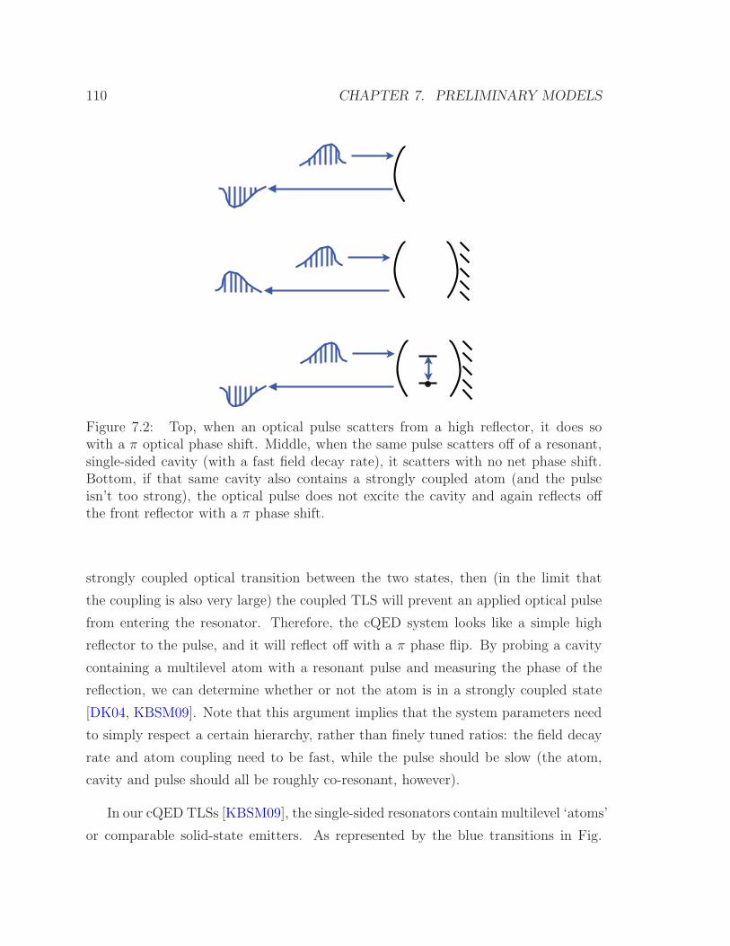
110 CHAPTER 7. PRELIMINARY MODELS
Figure 7.2: Top, when an optical pulse scatters from a high reflector, it does sowith a π optical phase shift. Middle, when the same pulse scatters off of a resonant,single-sided cavity (with a fast field decay rate), it scatters with no net phase shift.Bottom, if that same cavity also contains a strongly coupled atom (and the pulseisn’t too strong), the optical pulse does not excite the cavity and again reflects offthe front reflector with a π phase shift.
strongly coupled optical transition between the two states, then (in the limit that
the coupling is also very large) the coupled TLS will prevent an applied optical pulse
from entering the resonator. Therefore, the cQED system looks like a simple high
reflector to the pulse, and it will reflect off with a π phase flip. By probing a cavity
containing a multilevel atom with a resonant pulse and measuring the phase of the
reflection, we can determine whether or not the atom is in a strongly coupled state
[DK04, KBSM09]. Note that this argument implies that the system parameters need
to simply respect a certain hierarchy, rather than finely tuned ratios: the field decay
rate and atom coupling need to be fast, while the pulse should be slow (the atom,
cavity and pulse should all be roughly co-resonant, however).
In our cQED TLSs [KBSM09], the single-sided resonators contain multilevel ‘atoms’
or comparable solid-state emitters. As represented by the blue transitions in Fig.

7.2. CQED PARITY NETWORKS 111
a b
Figure 7.3: (from [KNPM10]) Atomic level diagrams of (a), Z probe interaction, (b)X probe interaction.
7.3, Z and X probe interactions emerge from a three level atomic system in a λ-
configuration interacting with a quantized mode of a single-sided cavity. In the case
of the Z probe, the |gy Ø |ey transition is strongly coupled and on resonance with
the cavity mode, while the |hy state is fully uncoupled. In the case of the X probe,
both |gy Ø |ey and |hy Ø |ey transitions are simultaneously coupled and on resonance
with the cavity mode. The X probe configuration could be realized with a degenerate
spin 1 ground state pair coupled to an excited spin-0 state via a linearly polarized
cavity mode, for example. Thus, in a properly rotating frame and applying the usual
rotating wave approximation, the familiar Jaynes-Cummings Hamiltonian interaction
for both systems is (section 3.1)
Hi igcpσ:a σa:q (7.14)
where a is the cavity mode annihilation operator, the atomic ‘lowering operators’ act
as σ |gyxe| on the atomic states in the Z-probe device, σ 1?2p|gy |hyq xe| in the
X-probe device, and the coupling rate gc may be taken real without loss of generality.
The remaining red optical transitions shown in Fig. 7.3 are for Raman interactions
discussed in the next chapter.
However, the cavity mode and atom also interact with the free fields that surround

112 CHAPTER 7. PRELIMINARY MODELS
them: the cavity photons will decay out of the resonator and the excited atomic
state will spontaneously emit photons into the environment. These interactions are
included in a QSDE description of the dynamics with the inclusion of two coupling
operators 1:
L1 ?2κa; L2 a2γKσ (7.15)
where κ and γK are the cavity field and atomic dipole decay rates, respectively. As
there is no direct coupling between the cavity and atomic decay channels, the scat-
tering matrix for this system is the identity. Thus, the QSDE descriptions of the
dynamics for the Z and X systems with vacuum inputs are characterized by the
operator coefficients (see section 1.5)
Q I,
?2κa?2γKσ
, igcpσ:a σa:q . (7.16)
I will eventually use the limiting evolution of these ‘vacuum’ cQED systems in the
network model, but note that familiar, driven cQED dynamics may be derived with
the inclusion of a Weyl operator (Eq. 1.33) in series product with the vacuum system
(representing an on-resonance, cw laser input to the cavity mode)
Qα QI, α
0
, 0
I,
?2κa α?2γKσ
, igcpσ:a σa:q i?κ
2pα:a αa:q, (7.17)
followed by the application of the master equation from section 1.3.
Rather than use the entire physical model for the cQED TLS given by Eq. (7.16)
in the network, I implement an adiabatic elimination procedure [BvHS08] (see section
1The physical system suggested for the X probe should actually include three coupling operators,as the state |ey may spontaneously emit right- or left-handed photons in a given direction. However,the proper inclusion of this additional decay channel leads to an equivalent limiting evolution.

7.2. CQED PARITY NETWORKS 113
1.6) on Q to obtain the very simple limiting dynamics of a measurable TLS, which
will be used in the network model. The physical intuition of the derived dynamics
is as follows. As described above and in [KBSM09, KNPM10], in a bad cavity limit
(κ Ñ 8), with the atom in a uncoupled state, a coherent probe resonant with the
cavity will enter the cavity and exit ‘immediately’ (due to the large κ), picking up no
additional phase shift. However, if the atom is in a coupled state, and the system is
also in a ‘small volume’ coupling limit (gc, κ Ñ 8 is expected as the device volume
vanishes), then the same probe will simply reflect from the off-resonant, atom-and-
cavity system, picking up an additional π phase shift. Thus, in these limits, the cQED
system acts as a simple scattering object with no internal dynamics, but which imparts
a phase shift on a cavity-incident coherent probe, as determined by the binary ground
state.
Following the mathematical formalism of [BvHS08], I redefine and relabel Q with
a scaling parameter k, which is assumed to take the limit k Ñ 8, and write the
component as a left QSDE (essentially the Hermitian conjugate of Q)
dQpkql,t Q
pkql,t
! k?2κadB1:
t k?2κa:dB1
ta2γKσdB2:
t a2γKσ:dB2t k2κa:adt γKσ:σdt
k2gcpσ:a σa:qdt). (7.18)
Note that with the scaling, the cavity field decay and coupling rates take the limits
described above (with gcκ constant).
In the notation of [BvHS08], the operator coefficients of the above left QSDE are
Kpkq k2κa:a γKσ:σ k2gca:σ aσ: ,
Lpkq k?2κa:?
2γKσ: , N pkq I.(7.19)
Through the adiabatic elimination procedure, a set of limiting operator coefficients
(denoted without the ‘pkq’) are derived, which define another, limiting propagator,
Ql,t, to which Qpkql,t strongly converges (see section 1.6). It is this limiting propagator
114 CHAPTER 7. PRELIMINARY MODELS
that will be used in the eventual network model in place of the physical cQED model.
For the adiabatic elimination we use (see section 1.6)
Y κa:a gca:σ aσ: , A 0, B γKσ:σ,
F ?2κa:
0
, G
0?2γKσ: , W I. (7.20)
In the Z probe case for the bit-flip network, H0 span t| g, 0y , |h, 0yu is the domain
of the ‘slow’ dynamics the adiabatic elimination procedure isolates and we define
Y t| g 0y , |h 0yu 0,
Y |hny 1
κn|hny , n ¥ 1;
Y | e pn 1qy gc?n
κ2n pn 1q g2cn| g ny
κn
κ2n pn 1q g2cn| e pn 1qy , n ¥ 1;
Y | g ny κ pn 1qκ2n pn 1q g2cn
| g nygc?n
κ2n pn 1q g2cn| e pn 1qy , n ¥ 1. (7.21)
which provides Y Y Y Y P1, the projector onto the complement of H0 (see section
1.6). Then by [BvHS08], the limiting operator coefficients are,
K 0, L1 L2 0, M1 M2 0, (7.22)

7.2. CQED PARITY NETWORKS 115
and (with Πin |i, nyxi, n|)N11 P0W11
F:1 Y F1 δ11
P0 P0 2κP0aY a
: pΠg0 Πh0q P0 2κP0aY p| g 1y xg 0| |h1y xh 0|q P0 2κP0a
1
gc| e 0y xg 0| 1
κ|h 1y xh 0| P0 2 |h 0y xh 0| Πg0 Πh0 Z,
N12 P0W11
F:1 Y F2 δ12
P0 0,
N21 P0W22
F:2 Y F1 δ21
P0 0,
N22 P0W22
F:2 Y F2 δ22
P0 1, (7.23)
Collecting the results, the limiting system (as a usual right-acting QSDE) is charac-
terized by the operator coefficients
Q Z 0
0 I
,
0
0
, 0
, (7.24)
to which the physical cQED system, Qpkq from Eq. (7.16), strongly converges in the
limit k Ñ 8. For the X probe case in the phase-flip network, the analogous follows,
but with the Pauli-X spin operator eventually replacing Z in equation (7.24).
7.2.2 Continuous parity measurement in a nanophotonic net-
work
Employing the series concatenation product (section 1.4), we can construct a QSDE
representation of a nanophotonic network in which two of these cQED TLSs are placed
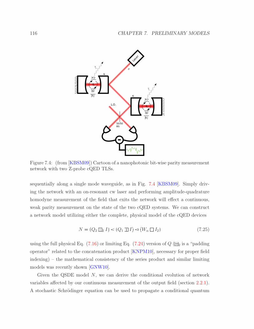
116 CHAPTER 7. PRELIMINARY MODELS
|h〉
|g〉
⊥
⊥
c
c
|h〉
|g〉
Figure 7.4: (from [KBSM09]) Cartoon of a nanophotonic bit-wise parity measurementnetwork with two Z-probe cQED TLSs.
sequentially along a single mode waveguide, as in Fig. 7.4 [KBSM09]. Simply driv-
ing the network with an on-resonant cw laser and performing amplitude-quadrature
homodyne measurement of the field that exits the network will effect a continuous,
weak parity measurement on the state of the two cQED systems. We can construct
a network model utilizing either the complete, physical model of the cQED devices
N pQ2 `2 Iq pQ1 ` Iq pWα ` I2q (7.25)
using the full physical Eq. (7.16) or limiting Eq. (7.24) version of Q (`2 is a “padding
operator” related to the concatenation product [KNPM10], necessary for proper field
indexing) – the mathematical consistency of the series product and similar limiting
models was recently shown [GNW10].
Given the QSDE model N , we can derive the conditional evolution of network
variables affected by our continuous measurement of the output field (section 2.2.1).
A stochastic Schrodinger equation can be used to propagate a conditional quantum

7.2. CQED PARITY NETWORKS 117
0 20 40 60 80 1000
0.2
0.4
0.6
0.8
1
|gg>
+ |
hh>
proj
ectio
n
Bell Expectations
0 20 40 60 80 100−0.5
0
0.5Homodyne Measurement Expectations
0 20 40 60 80 1000
0.2
0.4
0.6
0.8
1
|gh
> +
| h
g>
pro
ject
ion
0 20 40 60 80 100−0.5
0
0.5
time [units of (2γ )¯¹]
|gg> + |hh>
|gh> + |hg>
|gh> − |hg>
|gg> − |hh>
time [units of (2γ )¯¹]
<dY >t
Figure 7.5: (from [KBSM09]) Two independent simulations of atomic Bell-statepreparation in a realistic system (see text). The top pair of graphs show a simulationin which the system happened to reduce to even parity; the bottom pair shows anodd-parity example.
state derived from the continuous measurement records Mpiqt (where index piq speci-
fies the observed output channel). If the conditional state remains pure for all times
we may represent it by a vector |ψty. As complete purity of the conditional state
can only be achieved if all output channels are monitored with perfect efficiency, this
is not a realistic assumption in any actual implementation. However the equations
so derived are very useful for simulation and analysis; analogous equations for im-
perfect/incomplete observation with a mixed conditional state (density operator) are
easily derived as required for more practical purposes.
If we assume a Z-probe construction for Q and homodyne detection of the am-
plitude quadrature observable of the field that scatters off of both cavities Yp0qt
N:t pBt B
:t qNt jtpBt B
:t q, using Nt, the QSDE integral represented by the full
physical version of Eq. (7.25), and separate photon counting of each of the atomic ra-
diation modes Ypkqt jtpΛpkkq
t q k t1, 2u, the ‘physical’ pure-state propagator derived

118 CHAPTER 7. PRELIMINARY MODELS
from (7.25) is (section 2.2.1)
d|ψty #p?2κa1 ?2κa2 αqdY p0q
t g
2
i1
σpiq:ai σpiqa:idtpa:1a1 a
:2a2qκdt 2a:2a1κdt α
?2κpa1 a2q:dt 2
i1
pa2γKσpiq IqdY piqt γKσpiq:σpiqdt+|ψty. (7.26)
For simulation purposes Eq. (7.26) can be used to generate realistic homodyne mea-
surement records dYp0qt by driving the innovations and gauge processes with appro-
priate pseudo-random numbers (section 2.2.1 and [Tan99]). Similarly, if we define
jtpXq N:tXNt using the QSDE integral Nt represented by the limiting version of
Eq. (7.25) we can construct the ‘idealized’ pure state propagator assuming homodyne
measurement of Yt jtpBt B:t q as
d|ψty #αZ1Z2dYt |α|22dt
+|ψty, |ψ0y P H0 (7.27)
where Zi |hyxh||gyxg| on TLS i (note that for the limiting model for Q Eq. (7.24),
we don’t need to monitor the atomic radiation channels to maintain state purity).
It is straightforward to show that the idealized filter (7.27) represents a finite-time
unraveling of an ideal Z1Z2 projective measurement as discussed in [SvHM04]. As a
side note, it is interesting to point out that we can alternatively think of (7.27) as a
reduced filter for analyzing the homodyne photocurrent in a two-cavity setup, which
exploits adiabatic elimination for a reduction in the number of system variables. In
particular we could track the parity of the two ‘physical’ TLSs (approximately, but
with little computational effort) by driving (7.27) with an experimentally measured
homodyne photocurrent in place of dYt (see section 2.2.1). Below we will examine
the results of driving (7.27) with simulated ‘experimental’ photocurrents generated
by the physical Eq. (7.26).

7.2. CQED PARITY NETWORKS 119
To demonstrate that the physical model does realize an approximate parity mea-
surement, we can use (7.26) to simulate Bell-state entanglement generation from sep-
arable initial states of the atom-cavity systems [NC00], using parameters that should
be achievable in a Fabry-Perot cavity/cold Cs atom system with mm-scale dielectric
mirrors, tg, κ, γK, αu t20, 4.5, 0.5, 0.2u. We numerically integrate (7.26) from the
initial state |ψ0y 21pp|gy |hyq b |0yqb2 (that is, both cQED systems separably
in a superposition of the ground states and no photons in the cavity). As can be
seen in Fig. 7.5, the system begins with equal projections on the 212p|ggy |hhyqand 212p|ghy |hgyq joint atomic states and the expected homodyne photocurrent
vanishes. The laser is then adiabatically switched on and the conditional state grad-
ually projects into an atomic parity subspace with the corresponding xdY p0qt y 2α.
After a fixed time γKt 40 the probe is adiabatically switched off, but the projected
state persists. While the probe is on, the non-zero overlap with atomic Bell states not
present in the initial state is caused partially by entanglement with the cavity mode
states, but the residual expectation of such Bell states after the laser is switched off is
wholly due to the accumulation of weak measurements performed within the atomic
parity subspaces by the radiation field modes.
Finally, we compare the physical (7.26) and limiting (7.27) by two different com-
putational procedures. First, we compare independent simulations of the ideal-
ized projective measurement represented by Eq. (7.27) and the approximate pro-
jections represented by Eq. (7.26). To this end, we construct trajectories of the vari-
ance of parity operators: Varpσp1qZ σp2qZ q from |ψty in simulations of Eq. (7.26) (with
σZ |eyxe| |gyxg| |hyxh| distinguishing cavity-coupled and -uncoupled states),
and VarpZ1Z2q from |ψty in independent simulations of Eq. (7.27). Some summary
statistics from these simulations are depicted in Fig. 7.6. The integrations of the
idealized filter are initialized with |ψ0y 21p|gy |hyqb2. At t 0 we begin with
Varpσp1qZ σp2qZ q VarpZ1Z2q 1, and both variances decrease in time as the systems
randomly project into one parity subspace or the other. Indicative of their similar
statistics, the Varpσp1qZ σp2qZ q and VarpZ1Z2q trajectory ensembles largely overlap at all
times. Moreover, it can be shown that the excited state population remains small at
all times, pα?2κgq2, and that the atomic dynamics are principally constrained to the

120 CHAPTER 7. PRELIMINARY MODELS
two ground states.
Second, following up on our side note, we assess how well (7.27) performs as a
reduced filter for analyzing the physical system. In this case, we construct trajectories
of VarrfpZ1Z2q by integrating |ψty with photocurrents simulated from Eq. (7.26). A
representative VarrfpZ1Z2q,Varpσp1qZ σp2qZ q trajectory pair in Fig. 7.6 suggests the ac-
curacy of the reduced parity estimate. Underlaying this are the statistics of the frac-
tional residual error from 1000 such pairs: |Varpσp1qZ σp2qZ qVarrfpZ1Z2q|Varpσp1qZ σ
p2qZ q.
Although the range of Varpσp1qZ σp2qZ q spans 5 orders of magnitude, the reduced filter
performs well, tracking this physical parity estimate to within a factor of 2 in every
shot.

7.2. CQED PARITY NETWORKS 121
0 10 20 30 40 50 60 70 80 90 10010
−6
10−4
10−2
100
Physical vs. Ideal Parity Projection
Va
r rf(Ζ
Ζ 1 2 )
0 10 20 30 40 50 60 70 80 90 1000
0.2
0.4
0.6
0.8
1
Fra
ctio
na
l Re
sid
ua
l Err
or
0 10 20 30 40 50 60 70 80 90 10010
−6
10−4
10−2
100
Reduced Filter Performance
Va
r(σ
Z(1) σ
Z(2) ),
Var(Ζ Ζ1 2
)
Var(σZ
(1)σZ
(2))
time [units of (2γ )¯¹]
Figure 7.6: (from [KBSM09]) Summary of 1000 Bell-state projection simulations.The top graph compares the statistics of the ideal and physical parity variance. Themean of the Varpσp1qZ σ
p2qZ q trajectories is shown as a solid, black line; grey shading
indicates the one-standard deviation range of trajectories above and below the mean.The mean and standard deviation range of VarpZ1Z2q are shown by the dotted lineand blue shading. The bottom graph highlights the performance of the reduced filter.Referenced to the right axis, a representative Varpσp1qZ σ
p2qZ q, VarrfpZ1Z2q trajectory
pair are shown in solid black and dotted green, respectively. The blue-grey line andshading, referenced to the left axis, depicts the mean and standard deviation rangeof the fractional residual error over all trajectories.
Chapter 8
Autonomous QEC nanophotonic
networks
It’s well-established that quantum error correction (QEC) is critical to quantum in-
formation processing [NC00], but the usual formulation of error correction (e.g. see
section 7.1) entails a substantial overhead of classically controlled quantum operations
that is cumbersome to accommodate. In this section, I present a novel approach to
designing elementary QEC memory cells [KNPM10, KPCM11], in which all control
operations are performed autonomously by an embedded optical feedback loop. The
approach is natural for nanophotonic or superconducting microwave implementations
and in fact is expected to generally approach the ideal operation as the overall volume
of the system shrinks. The feedback network is entirely on-chip, requiring no external
clocking or control, and during steady-state operation would only need to be powered
by the injection of constant-amplitude coherent fields.
While the designs presented here are not yet possible to build, the network is
built from passive components such as optical waveguides, beamsplitters and cQED
devices, which have all shown rapid improvement in recent solid-state optical research
and should eventually be natural to integrate into large scale networks [PLP11,SBF10, KMV10, HKD09, FFE08]. Moreover, the details of the device imple-
mentation are of secondary importance. The specific designs were conceived of by
considering basic trends in device fabrication and the theoretical models available at
122
8.1. AN AUTONOMOUS BIT-/PHASE-FLIP NETWORK 123
this time. There are many different designs that could achieve these general goals. I
feel that the emphasis on designing quantum networks that control themselves and
the use of continuous-time physical modeling will be essential in developing actual
quantum technologies [JNP08, NJD09, Mab08a, IYY11, Mab11]. With QEC, even
in the abstract, this approach is also attractive for design and analysis because it
can connect the goal of quantum decoherence suppression with formal optimization
methods of classical control theory [ADL02, Mab09b].
While our approach exploits rigorous theoretical results derived using techniques
from quantum fields theory and coherent-feedback quantum control (part I), I first
give an intuitive presentation of a network that comprises five cavity QED devices and
emulates bit- or phase-flip QEC codes, depending on the configuration. That such
networks are naturally communicated both intuitively and formally (in the language
of QSDEs) suggests their general ability to bridge the gap between abstract quantum
information formulations and specific hardware implementations. The final section
builds off of the bit-/phase-flip network to propose a more powerful network capable
of protecting an encoded qubit from arbitrary single-TLS errors, demonstrating the
generalizability of the approach.
8.1 An autonomous bit-/phase-flip network
8.1.1 Intuitive operation
The photonic circuit shown in Fig. 8.1 implements continuous QEC [ADL02, Mab09b,
OLB08] based on the bit-flip or phase-flip code (section 7.1.1). Recall that in the bit-
flip code a single logical qubit is encoded in the joint state of three physical TLSs
and is protected against independent bit-flip errors on any of these register TLSs.
The logical state |0y is encoded by the physical state |000y (all three register TLSs
jointly in the ‘0’ state), while |1y is encoded by |111y. The analogous phase-flip code
associates |0y with |y and |1y with |y (where |y p|0y |1yq ?2) and the
logical qubit is protected against independent register phase-flip errors. In Fig. 8.1
Q1, Q2 and Q3 represent the register TLSs; the blue signal lines indicate the routing

124 CHAPTER 8. AUTONOMOUS QEC NANOPHOTONIC NETWORKS
Figure 8.1: (from [KNPM10]) Schematic diagram of an autonomous nanophotonicquantum memory showing TLSs in cavities (Q1, Q2 and Q3), circulators, beamsplit-ters, steering mirrors and relays.
of a laser beam (injected in the coherent state |2αy, where |α|2 has units photons
time1) used for error detection (following principles described in section 7.2.1); R1
and R2 represent two qubit-based photonic relays (as analyzed in [Mab09a]); and
the red signal lines indicate pathways for optical feedback using two additional laser
beams (injected in the coherent state |βy) for corrective Raman bit- or phase-flips.
The constant Hamiltonian interactions among the elementary physical systems along
the syndrome measurement pathway (blue signal lines) in Fig. 8.1 cause the |2αy fieldto be scattered into the inputs of the control relays R1 and R2 in such a way that
the relays correctly switch the routing of the optical power in the |βy feedback fields
(red signal lines) to perform a Raman bit flip or phase flip on any register qubit that
needs one. In this scheme α and β take the place of the usual discrete time interval
between executions of the circuit that implements syndrome measurement and unitary
restoration. Clocked execution of a special measurement/restoration circuit is not
required in this approach—with the physical component models described below,
the operation of the coherent controller is stationary in the sense that α, β and all
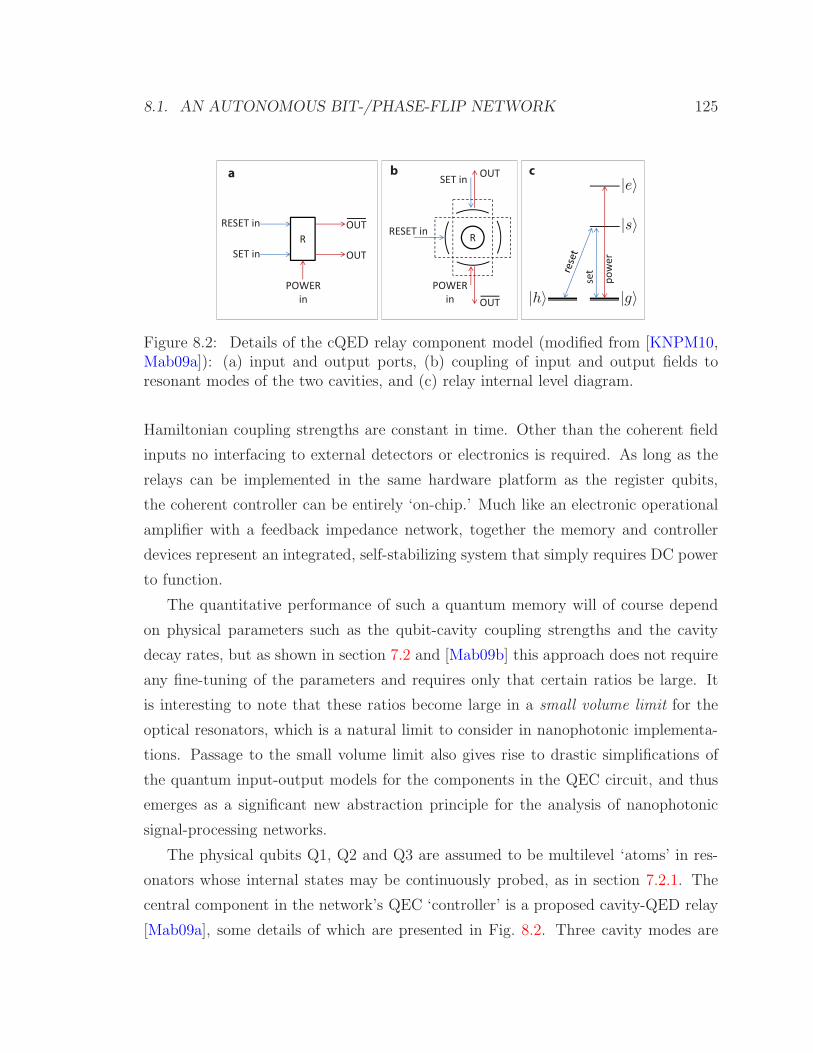
8.1. AN AUTONOMOUS BIT-/PHASE-FLIP NETWORK 125
a b c
Figure 8.2: Details of the cQED relay component model (modified from [KNPM10,Mab09a]): (a) input and output ports, (b) coupling of input and output fields toresonant modes of the two cavities, and (c) relay internal level diagram.
Hamiltonian coupling strengths are constant in time. Other than the coherent field
inputs no interfacing to external detectors or electronics is required. As long as the
relays can be implemented in the same hardware platform as the register qubits,
the coherent controller can be entirely ‘on-chip.’ Much like an electronic operational
amplifier with a feedback impedance network, together the memory and controller
devices represent an integrated, self-stabilizing system that simply requires DC power
to function.
The quantitative performance of such a quantum memory will of course depend
on physical parameters such as the qubit-cavity coupling strengths and the cavity
decay rates, but as shown in section 7.2 and [Mab09b] this approach does not require
any fine-tuning of the parameters and requires only that certain ratios be large. It
is interesting to note that these ratios become large in a small volume limit for the
optical resonators, which is a natural limit to consider in nanophotonic implementa-
tions. Passage to the small volume limit also gives rise to drastic simplifications of
the quantum input-output models for the components in the QEC circuit, and thus
emerges as a significant new abstraction principle for the analysis of nanophotonic
signal-processing networks.
The physical qubits Q1, Q2 and Q3 are assumed to be multilevel ‘atoms’ in res-
onators whose internal states may be continuously probed, as in section 7.2.1. The
central component in the network’s QEC ‘controller’ is a proposed cavity-QED relay
[Mab09a], some details of which are presented in Fig. 8.2. Three cavity modes are
126 CHAPTER 8. AUTONOMOUS QEC NANOPHOTONIC NETWORKS
resonant with various transitions in an intra-cavity atom, as shown in Fig. 8.2 (b)
and (c). In a similar small volume limit [Mab09a], the atomic dynamics are limited to
only the ground states, and when the atom is in state |hy (|gy) the cavity’s POWER
input is connected to the OUT (OUT) output port. A probe signal driving the SET
input port (in the absence of signal at the RESET input) causes the relay state to
decay to |hy, while driving only the RESET input induces decay to |gy. Through
these internal dynamics, a probe signal entering either the SET or RESET port of
the relay routes the POWER input out either the OUT or OUT port, respectively.
I now trace through the circuit dynamics of Fig. 8.1 in more detail, assuming a
bit-flip code implementation. A coherent input |2αy is split into probe and reference
beams. The probe beam first reflects from the cavity containing Q2, gaining a π or
0 phase shift depending on the state of that atom, putting the probe signal into a
coherent state with amplitude?2αZpQ2q (where ZpQ2q |hyxh| |gyxg| on Q2 and
the identity operation on all other Hilbert spaces is implied). The probe signal is
again split and the two resulting fields separately probe the cavities containing Q1
and Q3, resulting in signals with coherent amplitudes αZpQ1qZpQ2q and αZpQ2qZpQ3q.These are interfered with copies of the reference beam, producing four signals with
amplitudes αpIZpQ1qZpQ2qq?2 and αpIZpQ2qZpQ3qq?2. The ‘+’ signals are sent
to the SET inputs of relays R1 and R2, the ‘-’ to the RESET inputs. In this way,
the SET (RESET) input to R1 receives a coherent input signal if Q1 and Q2 have
even (odd) parity, while the RESET (SET) receives only a vacuum input. Similarly
for R2 and qubits Q2 and Q3. The POWER inputs to R1 and R2 are two more
coherent fields, each with amplitude β and frequency and polarization that drive the
remaining, far-detuned atomic transitions depicted in Fig. 7.3. The OUT port of R1
(R2) is directed to both Q1 and Q2 (Q2 and Q3). The OUT port of R1 (R2) is
directed to Q3 (Q1). When a qubit is simultaneously illuminated by two of these
feedback beams, Raman resonance conditions are satisfied, inducing a coherent Rabi
oscillation between the states of that single qubit. When only one feedback beam
illuminates an atom, the beam is assumed to be sufficiently detuned such that it only
imparts an AC Stark shift to one of the atomic ground states. Remarkably, a proper
choice of the ground state each feedback beam targets prevents Stark shift-induced
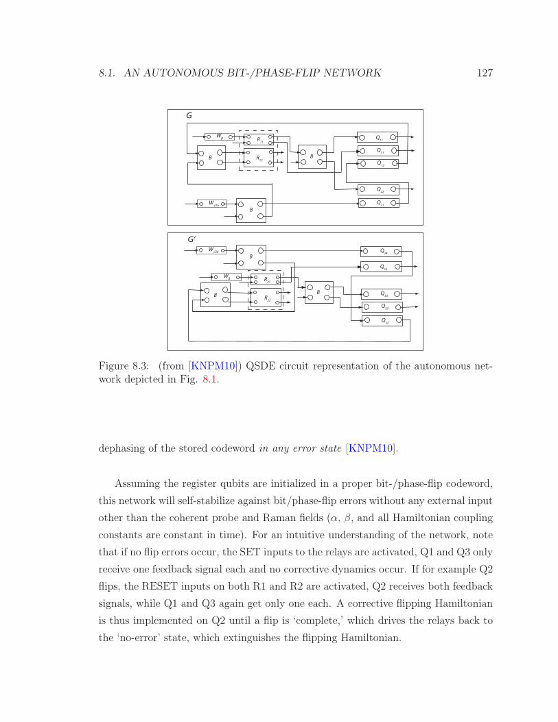
8.1. AN AUTONOMOUS BIT-/PHASE-FLIP NETWORK 127
B
B
Q11
Q13
Q12
Q32
Q31
Q33
Q24
Q23
Q22
Q21
B
B
B
B
G’
G
R12
R11
R22
R21
Wβ
Wβ
W√2α
W√2α
Figure 8.3: (from [KNPM10]) QSDE circuit representation of the autonomous net-work depicted in Fig. 8.1.
dephasing of the stored codeword in any error state [KNPM10].
Assuming the register qubits are initialized in a proper bit-/phase-flip codeword,
this network will self-stabilize against bit/phase-flip errors without any external input
other than the coherent probe and Raman fields (α, β, and all Hamiltonian coupling
constants are constant in time). For an intuitive understanding of the network, note
that if no flip errors occur, the SET inputs to the relays are activated, Q1 and Q3 only
receive one feedback signal each and no corrective dynamics occur. If for example Q2
flips, the RESET inputs on both R1 and R2 are activated, Q2 receives both feedback
signals, while Q1 and Q3 again get only one each. A corrective flipping Hamiltonian
is thus implemented on Q2 until a flip is ‘complete,’ which drives the relays back to
the ‘no-error’ state, which extinguishes the flipping Hamiltonian.

128 CHAPTER 8. AUTONOMOUS QEC NANOPHOTONIC NETWORKS
8.1.2 Network model and dynamics
A more schematic depiction of Fig. 8.1 appropriate for a QSDE representation of
the network is shown in Fig. 8.3. Static devices are now shown as labeled blocks,
with multiple I/O ports, while the fields connecting them are directional connections
between these ports. The QSDE component models are defined in the supplement of
[KNPM10], but Wα are coherent inputs (Weyl operators, section 1.4), B are beam-
splitters, Qij are the probe and Raman interaction subsystems of qubits Qi, and Rij
are subsystems of relay Ri.
The network considered in this section, shown schematically in 8.3 is slightly dif-
ferent from the network shown in Fig. 8.1. This is because in this more formal section,
the cavity for Q2 is taken to be two sided with a coherent probe laser impinging on
each side, allowing a decomposition of the network into two (symmetric) parts as
shown in Fig. 8.3 and simplifying the calculations for the overall network parameters.
On the other hand, in Fig. 8.1 all qubit cavities are identical and one sided, which
would be probably more suited in actual cQED implementations. Similar effects can
be achieved with either a double sided cavity for Q2 or a single sided cavity that is
followed by a 50/50 beamsplitter. Although the two networks are slightly different,
they only differ in the overall network scattering matrix, and a slightly modified re-
peat of the lengthy calculations, with Q2 one-sided and followed by a beamsplitter,
show that the network coupling vector and Hamiltonian will be the same for both
networks. As a consequence, I emphasize that the two networks will have the same
network master equation. Since, the main interest here is the network master equa-
tion, to derive this equation it is more convenient to work with the slightly modified
network of Fig. 8.3.
The unconditional master equation that describes the dynamics of the autonomous
network is immediately constructed after deriving the component model for G` G1,
8.1. AN AUTONOMOUS BIT-/PHASE-FLIP NETWORK 129
according to Fig. 8.3. First, following Fig. 8.3, the parts of G are
Gp R12 B ppQ12 Q21q` pI, 0, 0qq B W?
2α ` pI, 0, 0q ,Gf pQ11 `Q31 `Q22q pB `2 pI, 0, 0qq pR11 ` pI, 0, 0qq pWβ ` pI2, 0, 0qq , (8.1)
representing the ‘probe’ and ’feedback’ network subsystems of G Gp ` Gf , re-
spectively, and `2 is a “padding operator” related to the concatenation product
[KNPM10] (necessary for proper field indexing). Correspondences in G1 :R22 Ø R12, R21 Ø R11, Q23 Ø Q11, Q33 Ø Q22,
Q13 Ø Q31, Q24 Ø Q21, Q32 Ø Q12. (8.2)
The overall structure of the network is (with a trivial rearrangement of field indices)
N diagpSppq, S1ppq, Spfq, S1pfqq, Lppq
L1ppqLpfqL1pfq
,H ppq H 1ppq H pfq H 1pfq. (8.3)
In this calculation, the network components representing the bit- or phase-flips errors,
EpQiqX,Z , may be simply concatenated to the ‘correction’ network N immediately before
the derivation of the full system’s master equation.
A full, physical model for the network then follows from plugging in the physical
models for each of the W , B, Q, and R subsystems and applying the series and
concatenation products to obtain a single triplet, N pS, L,Hq network model. This
symbolic calculation may be done tediously by hand, but may also be automated
using symbolic matrix manipulation scripts. As the physical model utilizing both

130 CHAPTER 8. AUTONOMOUS QEC NANOPHOTONIC NETWORKS
the Q models derived in 7.2.1 for the probing component of Q1, Q2 and Q3 and the
full model for the Raman interactions are too cumbersome to analyze and too large
to simulate, we make use of the same adiabatic elimination theorem [BvHS08] to
consider instead the limiting dynamics as parameters are appropriately scaled. The
small volume limit may be taken before the network construction [GNW10], and so
the limiting version of Q model derived in section 7.2.1 (Eq. (7.24)) may be simply
plugged into N . The Raman interaction eliminates the excited state r in each qubit
(see Fig. 7.3) in the limit of large feedback amplitude and detuning. As the limiting
dynamics require input from both Gf and G1f components, this procedure may only
be done after N is at least partly constructed (see the supplemental of [KNPM10]).
After interconnecting simplified (small-volume) models for the bit-flip components
according to the bit-flip circuit diagram, including individual bit-flip error processes,
and adiabatically eliminating of all but the qubit and relay ground states, one obtains
[KNPM10] the closed-loop master equation9ρt irH, ρts 7
j1
LjρtL
j 1
2tLjLj , ρtu , (8.4)
where
H Ω
?2X pQ1qΠpR1q
g ΠpR2qh X pQ2qΠpR1q
g ΠpR2qg ?
2X pQ3qΠpR1qh ΠpR2q
g ΠpR1qg pΠpQ1q
g ΠpQ2qh q 2Π
pR1qh ΠpQ3q
g ΠpR2qg pΠpQ2q
g ΠpQ3qh q 2Π
pR2qh Π
pQ1qh
,
L1 α?2
ΠpR1qg Op12q σ
pR1qhg Ep12q , L2 α?
2
σpR1qgh Op12q ΠpR1qh Ep12q ,
L3 α?2
ΠpR2qg Op32q σ
pR2qhg Ep32q , L4 α?
2
σpR2qgh Op32q ΠpR2qh Ep32q ,
L5 ?ΓX pQ1q, L6 ?
ΓX pQ2q, L7 ?ΓX pQ3q (8.5)
where X pCq |hyxg| |gyxh|, σpCqjk |jyxk| and ΠpCqj |jyxj| on component C,
Epijq ZpQiqZpQjq 1 and Opijq ZpQiqZpQjq 1, each qubit suffers random flips at
a rate Γ, and the ‘feedback parameter’ Ω is proportional to |β|2∆ (note that several
Lj terms corresponding to strong dephasing of the relay states have been omitted

8.1. AN AUTONOMOUS BIT-/PHASE-FLIP NETWORK 131
0 0.02 0.04 0.06 0.08 .10.75
0.8
0.85
0.9
0.95
1
Γ t
Fid
elity
Ω = 0Ω = 10Ω = 60Ω = 110Ω = 160Ω = 210bare qubit
Figure 8.4: (from [KNPM10]) Decay of fidelity, xΨ0|ρt|Ψ0y, for several values of thefeedback parameter Ω |β|2γK2∆ (see the supplemental of [KNPM10]), α Ω8,and Γ 0.1. The fidelity decay of a single, bare qubit also suffering bitflip errors atrate Γ .1 is also shown.
as they have no appreciable effect on the dynamics). An analogous procedure using
the phase-flip component models leads to a master equation with the substitutions
ZpQiq Ø X pQiq, 2ΠpQiqhg
Ñ 1 X pQiq. While L5 through L7 drive the corrupting bit-
flip processes, the first three terms of the Hamiltonian (H) and remaining ‘collapse
operators’ work in concert to implement the corrections: L1 through L4 chiefly drive
the states of the two relays to reflect the qubit parities, and each bit-flipping term in
the Hamiltonian is only active for a particular ‘syndrome state’ [Got09], as indicated
by the relays. The remaining Hamiltonian terms physically correspond to AC Stark
shifts, whose effects have been minimized by design [KNPM10].
In Fig. 8.4 we display some illustrative numerical integrations [Tan99] of Eq. (8.4)
for the bit-flip scenario. With the flip rate set to Γ 0.1, the feedback amplitude is
varied from Ω 0 (no feedback) to Ω 210, with the probe amplitude kept at α Ω8. The initial state of the qubit register is chosen as |Ψ0y p|gggy i|hhhyq?2,

132 CHAPTER 8. AUTONOMOUS QEC NANOPHOTONIC NETWORKS
ρ0 |Ψ0yxΨ0|, and the fidelity decay xΨ0|ρt|Ψ0y is computed to quantify the deco-
herence suppression achieved by the coherent feedback loop. With Ω 0 the fidelity
decay is identical to that of the three-qubit register without any measurement or
feedback, while for larger values of Ω and longer storage times, the fidelity of the
encoded qubit is clearly improved relative to what it would be for a bare qubit. Vari-
able performance with |Ψ0y simply reflects the different susceptibilities of codewords
to bit-flip errors. Because of the small probability that additional errors accrue be-
fore the correction of a single flip, fidelity is gradually lost for finite probe/feedback
strengths, as in conventional QEC with finite correction time intervals.
8.2 The autonomous subsystem QEC network
While the network described in the previous section is able to emulate the bit- or
phase-flip QEC codes, such codes are severely limited: they can only protect the
encoded logical qubit against either single-qubit bit-flip or single-qubit phase-flip er-
rors. To emphasize how straightforwardly the approach scales to more powerful QEC
codes, in this final section I describe, model and simulate an autonomous nanopho-
tonic network that emulates the 9 qubit Bacon-Shor subsystem code [Bac06, AC07],
the smallest of a class of naturally fault-tolerant QEC codes capable of protecting a
single logical qubit from arbitrary single-qubit errors (see 7.1.2 for a description of
this code).
Using the same components and the intuition gained in section 8.1, it’s in fact
immediately clear how one could design a self-correcting nanophotonic network that
emulates the 9 qubit Bacon-Shor QEC code [Bac06]. In addition, one may also
immediately write down the full master equation that governs the internal dynamics
of all memory and controller devices of this network without having to resort to
a quantum circuit model, suggesting the general applicability of the approach (a
laborious, but straightforward network calculation confirms the master equation; see
below). In figure 8.5 we sketch the nanophotonic design. Two probe laser inputs first
travel down the middle row and column of a 3 3 grid of memory qubits. At the
end of the middle row or column, both probes are split on a beamsplitter with each
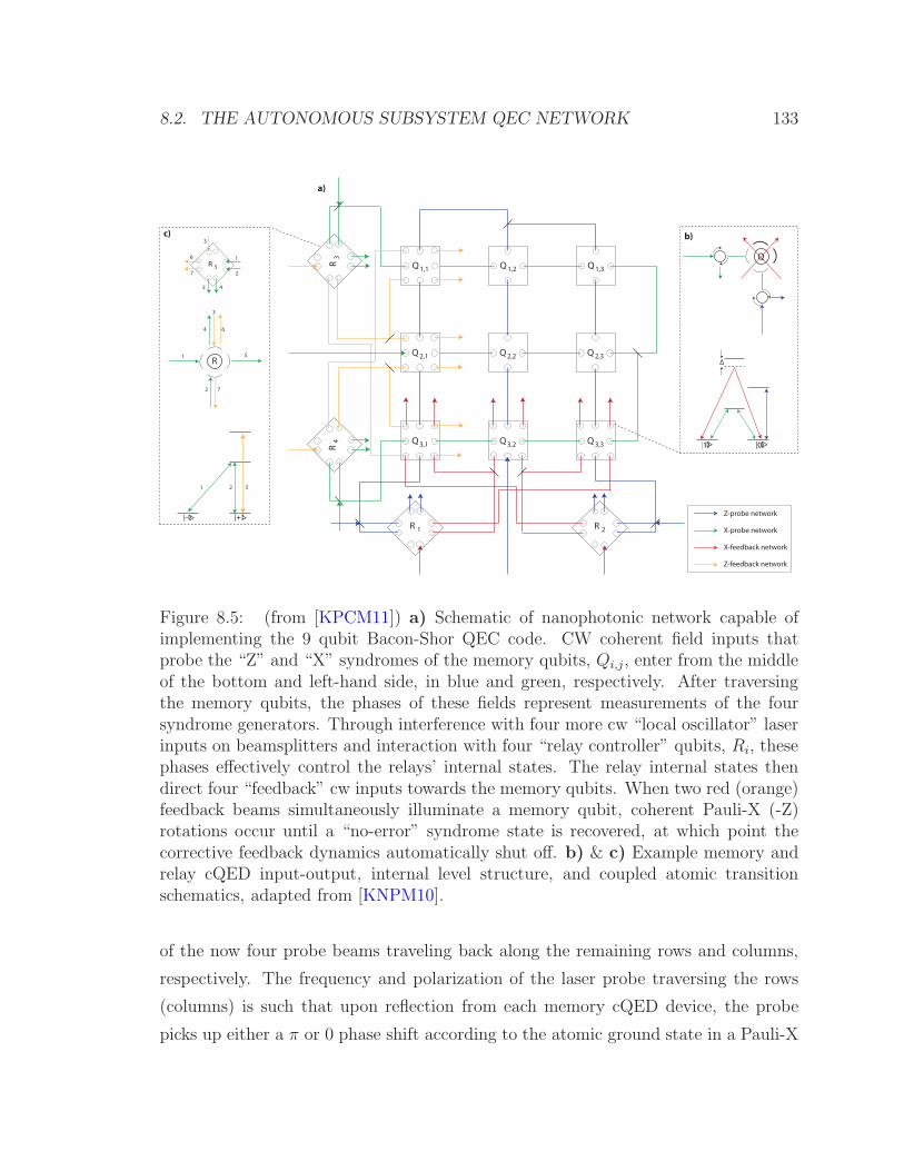
8.2. THE AUTONOMOUS SUBSYSTEM QEC NETWORK 133
Q 2,2
Q 1,2
Q 3,2Q 3,1
Q 1,3
Q 2,3
Q 3,3
Q 1,1
Q 2,1
R3
R4
R 1 R 2
a)
∆
Q
Z-probe network
X-probe network
X-feedback network
Z-feedback network
|1 |0
b)
R 3
1
2
3
45
6
7
1 2 3
1 5
4
3
6
72
R
|− |+
c)
> >
> >
Figure 8.5: (from [KPCM11]) a) Schematic of nanophotonic network capable ofimplementing the 9 qubit Bacon-Shor QEC code. CW coherent field inputs thatprobe the “Z” and “X” syndromes of the memory qubits, Qi,j, enter from the middleof the bottom and left-hand side, in blue and green, respectively. After traversingthe memory qubits, the phases of these fields represent measurements of the foursyndrome generators. Through interference with four more cw “local oscillator” laserinputs on beamsplitters and interaction with four “relay controller” qubits, Ri, thesephases effectively control the relays’ internal states. The relay internal states thendirect four “feedback” cw inputs towards the memory qubits. When two red (orange)feedback beams simultaneously illuminate a memory qubit, coherent Pauli-X (-Z)rotations occur until a “no-error” syndrome state is recovered, at which point thecorrective feedback dynamics automatically shut off. b) & c) Example memory andrelay cQED input-output, internal level structure, and coupled atomic transitionschematics, adapted from [KNPM10].
of the now four probe beams traveling back along the remaining rows and columns,
respectively. The frequency and polarization of the laser probe traversing the rows
(columns) is such that upon reflection from each memory cQED device, the probe
picks up either a π or 0 phase shift according to the atomic ground state in a Pauli-X

134 CHAPTER 8. AUTONOMOUS QEC NANOPHOTONIC NETWORKS
(Pauli-Z) basis. Thus after traversing the memory qubits, the phases of the four probe
lasers become entangled with the memory qubits via controlled-NOT interactions (in
a qubit Z- or X-basis) – essentially as four ancilla qubits would be to extract the
error syndrome in a measurement-based QEC scheme [Got09, NC00, AC07]. By
interfering with four local oscillator lasers, the phases of the four probes set the
internal state of four relays, which thus play the role of the classical register in a
measurement-based scheme; the four relay states together represent the quantum
memory’s error syndrome [Got09, NC00]. As in [KNPM10], these relays control
the routing of four more input “feedback” lasers that perform corrective, unitary
rotations on the ground state of the memory qubits via Raman interactions: when
a single qubit is simultaneously illuminated by feedback beams emitted by both “Z-
syndrome” (“X-syndrome”) relays, it undergoes coherent Pauli-X (Pauli-Z) rotations
between its ground states (for simplicity in this much larger network, we assume Stark-
shift compensation mechanisms are in place [KNPM10]) until the memory qubits –
followed by the controllers – recover their “no-error” state, and automatically shut
off the corrective feedback. Although errors may occur to any of memory qubits,
corrective feedback is applied to only a small subset of the memory qubits, as in
figure 8.5, due to the subsystem structure of the code [KLP05, Bac06] (see 7.1.2).
Moreover, as the internal states of the relays are continually reenforced by the cw
probes, errors in the relays’ atomic states should be self-corrected by the network.
The subsystem structure of the Bacon-Shor code [KLP05, Bac06] may be further
leveraged in a slightly modified network configuration. Although doing so would re-
quire a significantly more intricate waveguide network and/or cQED devices, instead
of threading the probe fields directly along rows and columns, a zig-zag configura-
tion, as in figure 8.6, should aid network robustness against optical waveguide loss.
Whereas photon loss almost anywhere in error-probe waveguide depicted in figure 8.5
effectively causes network-induced “errors” (which sometimes can be ameliorated by
the correction network), logical fidelity in the “zig-zag” network should be immune to
any waveguide loss in half of the probe network connections [AC07] (see 7.1.2). We
will consider these losses and other critical robustness concerns in depth a later pub-
lication, however, and so for my purposes here, both networks represented in figures
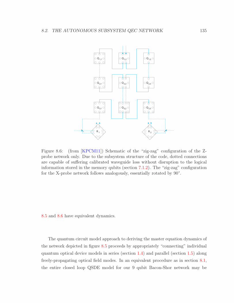
8.2. THE AUTONOMOUS SUBSYSTEM QEC NETWORK 135
Q 2,2
Q 1,2
Q 3,2Q 3,1
Q 1,3
Q 2,3
Q 3,3
Q 1,1
Q 2,1
R 1 R 2
Figure 8.6: (from [KPCM11]) Schematic of the “zig-zag” configuration of the Z-probe network only. Due to the subsystem structure of the code, dotted connectionsare capable of suffering calibrated waveguide loss without disruption to the logicalinformation stored in the memory qubits (section 7.1.2). The “zig-zag” configurationfor the X-probe network follows analogously, essentially rotated by 90.8.5 and 8.6 have equivalent dynamics.
The quantum circuit model approach to deriving the master equation dynamics of
the network depicted in figure 8.5 proceeds by appropriately “connecting” individual
quantum optical device models in series (section 1.4) and parallel (section 1.5) along
freely-propagating optical field modes. In an equivalent procedure as in section 8.1,
the entire closed loop QSDE model for our 9 qubit Bacon-Shor network may be

136 CHAPTER 8. AUTONOMOUS QEC NANOPHOTONIC NETWORKS
constructed from
GZp pRc
1 ` Rc2q pB ` Bq
QZ3,1 QZ
2,1 QZ1,1
` I1 ` QZ3,3 QZ
2,3 QZ1,3
ppB `2 I1q` I1q QZ1,2 QZ
2,2 QZ3,2 W
?2α`W α ` I1 `W α
Gf1
QX13,3 `QX1
3,1 `QX13,2
pI1 `Bq Rf1 W β ` I1
` I1
Gf2
QX13,1 `QX1
3,3 `QX13,2
pI1 `Bq Rf2 W β ` I1
` I1
GXp pRc
3 ` Rc4q pB ` Bq QX
1,1 QX1,2 QX
1,3
` I1 ` QX3,1 QX
3,2 QX3,3
ppB `2 I1q` I1q QX2,3 QX
2,2 QX2,1 W
?2α`W α ` I1 `W α
Gf3
QZ13,1 `QZ1
1,1 `QZ12,1
pI1 `Bq Rf3 W β ` I1
` I1
Gf4
QZ11,1 `QZ1
3,1 `QZ12,1
pI1 `Bq Rf4 W β ` I1
` I1
Gnetwork GZ
p `Gf1 `Gf2 `GXp `Gf3 `Gf4 (8.6)
where GZp (GX
p ) describes the “Z” (“X”) syndrome extraction network, Gfi describes
the feedback network controlled by relay i, and Gnetwork represents the pS, L,Hqtriple of the entire system, describing all but the error dynamics. As in the previous
section, the final step in the calculation, which yields a relatively low-dimensional total
network Gnetwork, is the application of an algorithmic adiabatic elimination procedure
[BvHS08] that restricts the Raman interaction dynamics to the ground states of the
memory qubits only.
Including arbitrary single-qubit dephasing of each memory qubit toGnetwork through
simple concatenation products, the closed loop dynamics of ρt, the density matrix for
all 9 memory and 4 relays qubits (physically representing the entire system’s dynam-
ics after tracing over the field degrees of freedom), is read off from the entire system’s

8.2. THE AUTONOMOUS SUBSYSTEM QEC NETWORK 137pS, L,Hq triple [KNPM10, Car93a], giving:9ρt irH, ρts 35
j1
LjρtL
j 1
2tLjLj , ρtu , with
H Ω
?2X3,1Π
1 Π
2 X3,2Π
1 Π
2 ?
2X3,3Π1 Π
2 ?
2Z1,1Π3 Π
4 Z2,1Π
3 Π
4 ?
2Z3,1Π3 Π
4
,
L1 α?2
Π
1 OZ1&2 σ1 EZ
1&2
, L2 α?
2
σ1 OZ1&2 Π
1 EZ1&2
,
L3 α?2
Π
2 OZ3&2 σ2 EZ
3&2
, L4 α?
2
σ2 OZ3&2 Π
2 EZ3&2
,
L5 α?2
Π
3 OX1&2 σ3 EX
1&2
, L6 α?
2
σ3 OX1&2 Π
3 EX1&2
,
L7 α?2
Π
4 OX3&2 σ4 EX
3&2
, L8 α?
2
σ4 OX3&2 Π
4 EX3&2
,
L917 ?ΓXi,j, L1826 ?
ΓZi,j, L2635 ?ΓYi,j i, j P Z3, (8.7)
where tXi,j, Zi,ju are the Pauli-tX,Zu operators on the memory qubit in row i and
column j, Πi is the projector onto state |y of relay i, σi |yx| for relay i, andtOZ
i&j, EZi&j,OX
i&j, OXi&j, u 1tZ,iZ,j, Z,iZ,j,Xi,Xj,, Xi,Xj,u with index signifying the operator product of all operators acting on some row or column. Γ
is the mean error rate of each type of single-qubit error, α is the coherent amplitude
of the (eventual) four probe lasers (where |α|2 has units photons time1), and Ω is
proportional to the optical power in each feedback beam. Comparison with the master
equation derived in the previous section Eq. (8.4), reveals that these dynamics for
the 9 qubit QEC subsystem code appear as an almost trivial expansion of that simple
bit-/phase-flip network.
Despite the idealized description of all cQED systems as simple qubits, Eq. (8.7)
still represents complex dynamics on a (sparse) density matrix with dimensions 294294. Due to the size of the problem, multi-threaded numerical integration of Eq.
(8.7) was carried out on a multicore computational server using BLAS routines with
OpenMP. Figure 8.7 depicts the time-evolution of the fidelity of the logical information
stored in the system, initialized with the logical qubit in the +1 YL eigenstate, the

138 CHAPTER 8. AUTONOMOUS QEC NANOPHOTONIC NETWORKS
0 0.01 0.02 0.03 0.04 0.05 0.06 0.07 0.08 0.09 0.10.5
0.55
0.6
0.65
0.7
0.75
0.8
0.85
0.9
0.95
1
Time [Γ t]
Fid
elity
Codeword fidelity decay
Ω = 0
Ω = 50
Ω = 100
Ω = 200
bare qubit
Figure 8.7: (from [KPCM11]) Decay of the logical codeword fidelity (see 7.1.2) intime for several feedback parameters. In the simulation, single-memory qubit X-, Y-and Z-errors occur each at average rate Γ .1 per qubit. While the amplitude of theprobes, are fixed at α Ω8, the feedback “strength” Ω is varied from 0 (no feedback)to 200. For large feedback strengths, the logical storage fidelity is eventually superiorto that of a single, bare qubit suffering arbitrary dephasing.
four gauge qubits in +1 ZT i eigenstates (see 7.1.2), and the four relays each in their
“no error” |y state. The bitwise-error rate was fixed at Γ .1, the probe strength
kept at α Ω8, and the “feedback strength” Ω varied from 0 to 200. Initially, all
fidelity curves drop steeply, representing a network “latency” before both probe and
feedback networks begin to correct errors. Thereafter, fidelity still drops due to the
finite probability that multiple errors irrecoverably accumulate before correction, but
at a retarded rate that decreases with increasing feedback strength. For Ω ¡ 100,
despite the initially steep fidelity loss, the decay is slow enough to eventually achieve
superior storage fidelity than a single, uncorrectable qubit suffering X-, Y-, and Z-
errors at the same bit-wise rate.
Finally, we may break down the dynamics of this particular network by calculating

8.2. THE AUTONOMOUS SUBSYSTEM QEC NETWORK 139
0 0.001 0.002 0.003 0.004 0.005 0.006 0.007 0.008 0.009 0.010.75
0.8
0.85
0.9
0.95
1QEC performance for different error classes
Time [Γ t]
FId
elity
X or Z errors
Y errors
All errors
All errors, Ω = 0
All errors, bare qubit
Figure 8.8: (from [KPCM11]) Comparison of network storage fidelity betweensystems suffering different types of errors. All solid curves are simulated withtΓ, α,Ωu t.1, 1008, 100u, except for the magenta curve, which has no feedback,as indicated. The blue curve represents the storage fidelity when only X- or onlyZ-errors occur to each memory qubit. The only slightly lower red curve comes from asystem suffering only Y-errors, which require coordination between all aspects of thenetwork. The green curve represents a system suffering all three types of error, eachat the same bit-wise rate, and has roughy the same fidelity decay as a sum of thedecays from each type of error acting alone. The dashed black line again representsthe logical fidelity of a single, bare qubit suffering all three types of errors at meanrate Γ .1 each.
its performance in response to different types of errors. In figure 8.8, we plot the
fidelity decay in time with tΓ, α,Ωu t.1, 1008, 100u, but with the memory qubits
suffering only single-qubit X-, Z-, or Y-errors. Systems suffering only X- or Z-errors
require only “half” of the feedback network to function well and achieve the best
storage fidelity. The system responds slightly worse to Y-errors. This is expected as
Y-flip errors (i.e. simultaneous bit-flip and phase-flip errors on a single qubit) requires
the two halves of the correction network to work in concert to correct the error. That
140 CHAPTER 8. AUTONOMOUS QEC NANOPHOTONIC NETWORKS
such coordination occurs without too much additional fidelity loss suggests that the
apparatus is fairly unbiased towards the types of errors it corrects. Similarly, when
all three errors are acting simultaneously, each at mean rate Γ .1 per qubit, the
additional fidelity loss scales roughly linearly with the total error rate in this strong
feedback regime, as one would expect for an efficiently operating system.

Bibliography
[AC91] P Alsing and H J Carmichael. Spontaneous dressed-state polarization
of a coupled atom and cavity mode. Quantum Optics: Journal of the
European Optical Society Part B, 3(1):13, 1991. Available from: http://
stacks.iop.org/0954-8998/3/i=1/a=003. 52, 55, 58, 60, 91
[AC07] Panos Aliferis and Andrew W. Cross. Subsystem fault tolerance with
the bacon-shor code. Phys. Rev. Lett., 98(22):220502, May 2007.
doi:10.1103/PhysRevLett.98.220502. 109, 132, 134
[ADL02] Charlene Ahn, Andrew C. Doherty, and Andrew J. Landahl. Continuous
quantum error correction via quantum feedback control. Phys. Rev. A,
65(4):042301, Mar 2002. doi:10.1103/PhysRevA.65.042301. 123
[AM06] M. A. Armen and H. Mabuchi. Low-lying bifurcations in cavity
quantum electrodynamics. Phys. Rev. A, 73(6):063801, Jun 2006.
doi:10.1103/PhysRevA.73.063801. 37, 39, 44, 45, 46, 48, 49
[AMM09] Michael A. Armen, Anthony E. Miller, and Hideo Mabuchi. Spon-
taneous dressed-state polarization in the strong driving regime
of cavity qed. Phys. Rev. Lett., 103(17):173601, Oct 2009.
doi:10.1103/PhysRevLett.103.173601. 52, 55, 75, 76, 91, 95
[Arm09] M. A. Armen. Bifurcations in single-atom cavity QED. PhD thesis,
California Institute of Technology, 2009. 40, 41, 52, 55, 57, 58, 70, 73,
74, 75, 76, 91, 95
141
142 BIBLIOGRAPHY
[ASO08] Peter A. Andrekson, Henrik Sunnerud, Shoichiro Oda, Takashi
Nishitani, and Jiang Yang. Ultrafast, atto-joule switch using
fiber-opticparametric amplifier operated in saturation. Opt. Ex-
press, 16(15):10956–10961, Jul 2008. Available from: http://
www.opticsexpress.org/abstract.cfm?URI=oe-16-15-10956,
doi:10.1364/OE.16.010956. 47, 69
[Bac06] Dave Bacon. Operator quantum error-correcting subsystems for self-
correcting quantum memories. Phys. Rev. A, 73(1):012340, Jan 2006.
doi:10.1103/PhysRevA.73.012340. 107, 132, 134
[Bar90] A Barchielli. Direct and heterodyne detection and other applications of
quantum stochastic calculus to quantum optics. Quantum Optics: Jour-
nal of the European Optical Society Part B, 2(6):423, 1990. Available
from: http://stacks.iop.org/0954-8998/2/i=6/a=002. 4, 6, 10, 14,
23, 24, 26, 28
[BFSB09] Paul E. Barclay, Kai-Mei Fu, Charles Santori, and Raymond G.
Beausoleil. Hybrid photonic crystal cavity and waveguide for cou-
pling to diamond nv-centers. Opt. Express, 17(12):9588–9601, Jun
2009. Available from: http://www.opticsexpress.org/abstract.
cfm?URI=oe-17-12-9588, doi:10.1364/OE.17.009588. 38
[BMB04] A. Boca, R. Miller, K. M. Birnbaum, A. D. Boozer, J. McK-
eever, and H. J. Kimble. Observation of the vacuum rabi spectrum
for one trapped atom. Phys. Rev. Lett., 93(23):233603, Dec 2004.
doi:10.1103/PhysRevLett.93.233603. 36, 73
[BvHJ07] Luc Bouten, Ramon van Handel, and Matthew R. James. An introduc-
tion to quantum filtering. SIAM Journal on Control and Optimization,
46(6):2199–2241, 2007. Available from: http://link.aip.org/link/?
SJC/46/2199/1, doi:10.1137/060651239. 4, 6, 10, 13, 14, 15, 23, 24,
26, 31, 32, 33, 34

BIBLIOGRAPHY 143
[BvHS08] Luc Bouten, Ramon van Handel, and Andrew Silberfarb. Approxima-
tion and limit theorems for quantum stochastic models with unbounded
coefficients. Journal of Functional Analysis, 254(12):3123 – 3147,
2008. Available from: http://www.sciencedirect.com/science/
article/B6WJJ-4S69SFK-1/2/1f6713358ce099d9ea560a15cbdf84eb,
doi:DOI:10.1016/j.jfa.2008.02.013. 4, 6, 20, 21, 112, 113, 114,
130, 136
[Car93a] H. Carmichael. An Open Systems Approach to Quantum Optics.
Springer Berlin / Heidelberg, 1993. 16, 23, 24, 31, 33, 36, 37, 39, 40, 42,
73, 137
[Car93b] H. J. Carmichael. Frontiers in Optics. Springer-Verlag, Berlin, 1993. 44
[CLS04] J. Chiaverini, D. Leibfried, T. Schaetz, M. D. Barrett, R. B. Blakestad,
J. Britton, W. M. Itano, J. D. Jost, E. Knill, C. Langer, R. Ozeri,
and D. J. Wineland. Realization of quantum error correction. Nature,
432(7017):602–605, 12 2004. Available from: http://dx.doi.org/10.
1038/nature03074. 99
[CMR05] O. Cappe, E. Moulines, and T. Ryden. Inference in Hidden Markov
Models. Springer, 2005. 92
[CTDRG89] C. Cohen-Tannoudji, J. Dupont-Roc, and G. Grynberg. Photons &
Atoms: Introduction to Quantum Electrodynamics. John Wiley & Sons,
Inc., 1989. 38, 40
[CTDRG92] C. Cohen-Tannoudji, J. Dupont-Roc, and G. Grynberg. Atom-Photon
Interactions: Basic Processes and Applications. John Wiley & Sons,
Inc., 1992. 38, 39
[DCG09] L. DiCarlo, J. M. Chow, J. M. Gambetta, Lev S. Bishop, B. R. John-
son, D. I. Schuster, J. Majer, A. Blais, L. Frunzio, S. M. Girvin, and
144 BIBLIOGRAPHY
R. J. Schoelkopf. Demonstration of two-qubit algorithms with a su-
perconducting quantum processor. Nature, 460(7252):240–244, 07 2009.
Available from: http://dx.doi.org/10.1038/nature08121. 99
[DHK83] R. W. P. Drever, J. L. Hall, F. V. Kowalski, J. Hough, G. M. Ford, A. J.
Munley, and H. Ward. Laser phase and frequency stabilization using
an optical resonator. Applied Physics B: Lasers and Optics, 31:97–105,
1983. 10.1007/BF00702605. Available from: http://dx.doi.org/10.
1007/BF00702605. 76
[DK04] L.-M. Duan and H. J. Kimble. Scalable photonic quantum computation
through cavity-assisted interactions. Phys. Rev. Lett., 92(12):127902,
Mar 2004. doi:10.1103/PhysRevLett.92.127902. 110
[DRS10] L. DiCarlo, M. D. Reed, L. Sun, B. R. Johnson, J. M. Chow, J. M. Gam-
betta, L. Frunzio, S. M. Girvin, M. H. Devoret, and R. J. Schoelkopf.
Preparation and measurement of three-qubit entanglement in a super-
conducting circuit. Nature, 467(7315):574–578, 09 2010. Available from:
http://dx.doi.org/10.1038/nature09416. 99
[EFF07] Dirk Englund, Andrei Faraon, Ilya Fushman, Nick Stoltz, Pierre Petroff,
and Jelena Vuckovic. Controlling cavity reflectivity with a single quan-
tum dot. Nature, 450(7171):857–861, 12 2007. Available from: http://
dx.doi.org/10.1038/nature06234. 55
[EFZ07] Dirk Englund, Andrei Faraon, Bingyang Zhang, Yoshihisa Yamamoto,
and Jelena Vuckovic. Generation and transfer of single photons
on a photonic crystal chip. Opt. Express, 15(9):5550–5558, Apr
2007. Available from: http://www.opticsexpress.org/abstract.
cfm?URI=oe-15-9-5550, doi:10.1364/OE.15.005550. 36, 38
[Fag90] Franco Fagnola. On quantum stochastic differential equations with un-
bounded coefficients. Probability Theory and Related Fields, 86:501–516,

BIBLIOGRAPHY 145
1990. 10.1007/BF01198172. Available from: http://dx.doi.org/10.
1007/BF01198172. 4
[FFE08] Andrei Faraon, Ilya Fushman, Dirk Englund, Nick Stoltz, Pierre Petroff,
and Jelena Vuckovic. Dipole induced transparency in waveguide cou-
pled photonic crystal cavities. Opt. Express, 16(16):12154–12162, Aug
2008. Available from: http://www.opticsexpress.org/abstract.
cfm?URI=oe-16-16-12154, doi:10.1364/OE.16.012154. 122
[FMK10] Andrei Faraon, Arka Majumdar, Hyochul Kim, Pierre Petroff, and Je-
lena Vuckovic. Fast electrical control of a quantum dot strongly coupled
to a photonic-crystal cavity. Phys. Rev. Lett., 104(4):047402, Jan 2010.
doi:10.1103/PhysRevLett.104.047402. 67, 68
[FSS10] J. M. Fink, L. Steffen, P. Studer, Lev S. Bishop, M. Baur, R. Bianchetti,
D. Bozyigit, C. Lang, S. Filipp, P. J. Leek, and A. Wallraff. Quantum-to-
classical transition in cavity quantum electrodynamics. Phys. Rev. Lett.,
105(16):163601, Oct 2010. doi:10.1103/PhysRevLett.105.163601. 36,
55, 58
[Gar04] C. W. Gardiner. Handbook of Stochastic Methods. Springer, 2004. 10,
11, 12, 16, 20, 21
[GJ09a] J. Gough and M. James. Quantum feedback networks: Hamiltonian for-
mulation. Communications in Mathematical Physics, 287:1109–1132,
2009. 10.1007/s00220-008-0698-8. Available from: http://dx.doi.
org/10.1007/s00220-008-0698-8. 17
[GJ09b] J. Gough and M.R. James. The series product and its ap-
plication to quantum feedforward and feedback networks. Auto-
matic Control, IEEE Transactions on, 54(11):2530 –2544, nov. 2009.
doi:10.1109/TAC.2009.2031205. 4, 6, 15, 17, 18, 19
146 BIBLIOGRAPHY
[GNH90a] Hu Gang, Cun-Zheng Ning, and H. Haken. Codimension-two bifurca-
tions in single-mode optical bistable systems. Phys. Rev. A, 41(5):2702–
2711, Mar 1990. doi:10.1103/PhysRevA.41.2702. 45, 46
[GNH90b] Hu Gang, Cun-Zheng Ning, and H. Haken. Distribution of sub-
critical hopf bifurcations and regular and chaotic attractors in op-
tical bistable systems. Phys. Rev. A, 41(7):3975–3984, Apr 1990.
doi:10.1103/PhysRevA.41.3975. 45, 46
[GNW10] John E. Gough, Hendra I. Nurdin, and Sebastian Wildfeuer. Com-
mutativity of the adiabatic elimination limit of fast oscillatory com-
ponents and the instantaneous feedback limit in quantum feed-
back networks. Journal of Mathematical Physics, 51(12):123518,
2010. Available from: http://link.aip.org/link/?JMP/51/123518/
1, doi:10.1063/1.3520513. 116, 130
[Got09] D. Gottesman. An Introduction to Quantum Error Correction and
Fault-Tolerant Quantum Computation. ArXiv e-prints, April 2009.
arXiv:0904.2557. 100, 102, 104, 107, 131, 134
[GPZ92] C. W. Gardiner, A. S. Parkins, and P. Zoller. Wave-function
quantum stochastic differential equations and quantum-jump sim-
ulation methods. Phys. Rev. A, 46(7):4363–4381, Oct 1992.
doi:10.1103/PhysRevA.46.4363. 4, 6, 7, 8, 9, 10, 11, 12, 13, 14, 31
[GZ04] C. W. Gardiner and P. Zoller. Quantum Noise: A Hanbook of Markovian
and Non-Markovian Quantum Stochastic Methods with Applications to
Quantum Optics. Springer, 2004. 4, 6, 8, 9, 10, 11, 12, 14, 15, 16, 17,
23, 24, 26, 31, 33, 40, 42
[HCLK98] C. J. Hood, M. S. Chapman, T. W. Lynn, and H. J. Kimble. Real-time
cavity qed with single atoms. Phys. Rev. Lett., 80(19):4157–4160, May
1998. doi:10.1103/PhysRevLett.80.4157. 51, 54, 55, 72
BIBLIOGRAPHY 147
[HKD09] A. Houck, Jens Koch, M. Devoret, S. Girvin, and R. Schoelkopf. Life
after charge noise: recent results with transmon qubits. Quantum Infor-
mation Processing, 8:105–115, 2009. 10.1007/s11128-009-0100-6. Avail-
able from: http://dx.doi.org/10.1007/s11128-009-0100-6. 71, 122
[HKY01] Christina J. Hood, H. J. Kimble, and Jun Ye. Characteriza-
tion of high-finesse mirrors: Loss, phase shifts, and mode struc-
ture in an optical cavity. Phys. Rev. A, 64(3):033804, Aug 2001.
doi:10.1103/PhysRevA.64.033804. 73
[HP84] R. L. Hudson and K. R. Parthasarathy. Quantum ito’s formula
and stochastic evolutions. Communications in Mathematical Physics,
93:301–323, 1984. 10.1007/BF01258530. Available from: http://dx.
doi.org/10.1007/BF01258530. 4, 12, 13
[IYY11] S. Iida, M. Yukawa, H. Yonezawa, N. Yamamoto, and A. Furusawa.
Experimental demonstration of coherent feedback control on optical field
squeezing. ArXiv e-prints, March 2011. arXiv:1103.1324. 123
[JNP08] M.R. James, H.I. Nurdin, and I.R. Petersen. h8 control of linear quan-
tum stochastic systems. Automatic Control, IEEE Transactions on,
53(8):1787 –1803, sept. 2008. doi:10.1109/TAC.2008.929378. 4, 123
[KAM10] J. Kerckhoff, M. A. Armen, and H. Mabuchi. Quantum remnants of
absorptive bistability in the attojoule regime. ArXiv e-prints, December
2010. arXiv:1012.4873. 37, 45, 48, 84, 85, 86, 87, 88, 89
[KAPM11] Joseph Kerckhoff, Michael A. Armen, Dmitri S. Pavlichin, and Hideo
Mabuchi. The dressed atom as binary phase modulator: towards
attojoule/edge optical phase-shift keying. Opt. Express, 19(7):6478–
6486, Mar 2011. Available from: http://www.opticsexpress.org/
abstract.cfm?URI=oe-19-7-6478, doi:10.1364/OE.19.006478. 37,
55, 61, 68, 84, 90, 92, 93, 97

148 BIBLIOGRAPHY
[KBSM09] Joseph Kerckhoff, Luc Bouten, Andrew Silberfarb, and Hideo
Mabuchi. Physical model of continuous two-qubit parity measure-
ment in a cavity-qed network. Phys. Rev. A, 79(2):024305, Feb 2009.
doi:10.1103/PhysRevA.79.024305. 109, 110, 113, 116, 117, 121
[KLP05] David Kribs, Raymond Laflamme, and David Poulin. Unified and
generalized approach to quantum error correction. Phys. Rev. Lett.,
94(18):180501, May 2005. doi:10.1103/PhysRevLett.94.180501. 106,
134
[KMV10] H. S. Ku, F. Mallet, L. R. Vale, K. D. Irwin, S. E. Russek, G. C.
Hilton, and K. W. Lehnert. Design and testing of superconducting
microwave passive components for quantum information processing.
Applied Superconductivity, IEEE Transactions on, PP(99):1 –4, 2010.
doi:10.1109/TASC.2010.2089403. 122
[KNPM10] Joseph Kerckhoff, Hendra I. Nurdin, Dmitri S. Pavlichin, and Hideo
Mabuchi. Designing quantum memories with embedded control: Pho-
tonic circuits for autonomous quantum error correction. Phys. Rev. Lett.,
105(4):040502, Jul 2010. doi:10.1103/PhysRevLett.105.040502. 4,
18, 19, 21, 99, 111, 113, 116, 122, 124, 125, 127, 128, 129, 130, 131, 133,
134, 137
[KPCM11] J. Kerckhoff, D. S. Pavlichin, H. Chalabi, and H. Mabuchi. Design of
nanophotonic circuits for autonomous subsystem quantum error correc-
tion. ArXiv e-prints, to appear in New J. Phys. (special issue Integrated
Quantum Optics), February 2011. arXiv:1102.3143. 21, 99, 122, 133,
135, 138, 139
[LKH10] Liu Liu, Rajesh Kumar, Koen Huybrechts, Thijs Spuesens, Gunther
Roelkens, Erik-Jan Geluk, Tjibbe de Vries, Philippe Regreny, Dries
Van Thourhout, Roel Baets, and Geert Morthier. An ultra-small,
low-power, all-optical flip-flop memory on a silicon chip. Nat Photon,

BIBLIOGRAPHY 149
4(3):182–187, 03 2010. Available from: http://dx.doi.org/10.1038/
nphoton.2009.268. 47, 69
[Lug84] L. A. Lugiato. Progress in Optics. North-Holland, Amsterdam, 1984.
44
[Mab08a] Hideo Mabuchi. Coherent-feedback quantum control with a dy-
namic compensator. Phys. Rev. A, 78(3):032323, Sep 2008.
doi:10.1103/PhysRevA.78.032323. 123
[Mab08b] Hideo Mabuchi. Derivation of maxwell-bloch-type equations by pro-
jection of quantum models. Phys. Rev. A, 78(1):015801, Jul 2008.
doi:10.1103/PhysRevA.78.015801. 45
[Mab09a] Hideo Mabuchi. Cavity-qed models of switches for attojoule-
scale nanophotonic logic. Phys. Rev. A, 80(4):045802, Oct 2009.
doi:10.1103/PhysRevA.80.045802. 124, 125, 126
[Mab09b] Hideo Mabuchi. Continuous quantum error correction as classical hybrid
control. New Journal of Physics, 11(10):105044, 2009. Available from:
http://stacks.iop.org/1367-2630/11/i=10/a=105044. 123, 125
[Mab11] H. Mabuchi. Coherent-feedback control strategy to suppress sponta-
neous switching in ultra-low power optical bistability. ArXiv e-prints,
January 2011. arXiv:1101.3461. 123
[MD02] H. Mabuchi and A. C. Doherty. Cavity quantum electrodynamics: Co-
herence in context. Science, 298(5597):1372–1377, 2002. Available from:
http://www.sciencemag.org/content/298/5597/1372.abstract,
arXiv:http://www.sciencemag.org/content/298/5597/1372.full.pdf,
doi:10.1126/science.1078446. 36, 37
[Mil09] D. Miller. Device requirements for optical interconnects to sili-
con chips. Proceedings of the IEEE, 97(7):1166 –1185, july 2009.
doi:10.1109/JPROC.2009.2014298. 48

150 BIBLIOGRAPHY
[Mil10a] David A. B. Miller. Are optical transistors the logical next step? Nat
Photon, 4(1):3–5, 01 2010. Available from: http://dx.doi.org/10.
1038/nphoton.2009.240. 48
[Mil10b] David A. B. Miller. Optical interconnects to electronic chips. Appl.
Opt., 49(25):F59–F70, Sep 2010. Available from: http://ao.osa.org/
abstract.cfm?URI=ao-49-25-F59, doi:10.1364/AO.49.000F59. 50
[Moo05] K. L. Moore. Ultracold Atoms, Circular Waveguides, and Cavity QED
with Milli-meter-scale Electromagnetic Traps. PhD thesis, University of
California, Berkeley, 2005. 74
[MTCK96] H. Mabuchi, Q. A. Turchette, M. S. Chapman, and H. J. Kim-
ble. Real-time detection of individual atoms falling through a high-
finesse optical cavity. Opt. Lett., 21(17):1393–1395, Sep 1996. Avail-
able from: http://ol.osa.org/abstract.cfm?URI=ol-21-17-1393,
doi:10.1364/OL.21.001393. 36, 72
[MvdS99] H. J. Metcalf and P. van der Straten. Laser Cooling and Trapping.
Springer, 1999. 80
[NC00] M. A. Nielsen and I. L. Chuang. Quantum Computation and Quanutm
Information. Cambridge University Press, 2000. 99, 100, 102, 104, 105,
107, 119, 122, 134
[NJD09] Hendra I. Nurdin, Matthew R. James, and Andrew C. Doherty.
Network synthesis of linear dynamical quantum stochastic sys-
tems. SIAM Journal on Control and Optimization, 48(4):2686–2718,
2009. Available from: http://link.aip.org/link/?SJC/48/2686/1,
doi:10.1137/080728652. 4, 123
[NJP09] Hendra I. Nurdin, Matthew R. James, and Ian R. Petersen. Co-
herent quantum lqg control. Automatica, 45(8):1837 – 1846,
2009. Available from: http://www.sciencedirect.com/science/
BIBLIOGRAPHY 151
article/B6V21-4WK4B3T-1/2/70c6e071f68558e9690d6fe9cbfb10f0,
doi:DOI:10.1016/j.automatica.2009.04.018. 4
[NTS10] Kengo Nozaki, Takasumi Tanabe, Akihiko Shinya, Shinji Matsuo,
Tomonari Sato, Hideaki Taniyama, and Masaya Notomi. Sub-femtojoule
all-optical switching using a photonic-crystal nanocavity. Nat Photon,
4(7):477–483, 07 2010. Available from: http://dx.doi.org/10.1038/
nphoton.2010.89. 47, 69
[OLB08] Ognyan Oreshkov, Daniel A. Lidar, and Todd A. Brun. Operator
quantum error correction for continuous dynamics. Phys. Rev. A,
78(2):022333, Aug 2008. doi:10.1103/PhysRevA.78.022333. 123
[ORX87] L. A. Orozco, M. G. Raizen, Min Xiao, R. J. Brecha, and
H. J. Kimble. Squeezed-state generation in optical bistabil-
ity. J. Opt. Soc. Am. B, 4(10):1490–1550, Oct 1987. Available
from: http://josab.osa.org/abstract.cfm?URI=josab-4-10-1490,
doi:10.1364/JOSAB.4.001490. 72
[Par92] K. R. Parthasarathy. An Introduction to Quantum Stochastic Calculus.
Birkhauser, Berlin, 1992. 4, 12, 13
[PLP11] Alberto Peruzzo, Anthony Laing, Alberto Politi, Terry Rudolph, and
Jeremy L. O’Brien. Multimode quantum interference of photons in mul-
tiport integrated devices. Nat Commun, 2, 03 2011. Available from:
http://dx.doi.org/10.1038/ncomms1228. 122
[PLZY08] David Press, Thaddeus D. Ladd, Bingyang Zhang, and Yoshihisa Ya-
mamoto. Complete quantum control of a single quantum dot spin using
ultrafast optical pulses. Nature, 456(7219):218–221, 11 2008. Available
from: http://dx.doi.org/10.1038/nature07530. 71
[PMO09] Alberto Politi, Jonathan C. F. Matthews, and Jeremy L.
O’Brien. Shor’s quantum factoring algorithm on a pho-
tonic chip. Science, 325(5945):1221, 2009. Available from:

152 BIBLIOGRAPHY
http://www.sciencemag.org/content/325/5945/1221.abstract,
arXiv:http://www.sciencemag.org/content/325/5945/1221.full.pdf,
doi:10.1126/science.1173731. 99
[PSK08] T.P. Purdy and D.M. Stamper-Kurn. Integrating cavity quantum elec-
trodynamics and ultracold-atom chips with on-chip dielectric mirrors
and temperature stabilization. Applied Physics B: Lasers and Optics,
90:401–405, 2008. 10.1007/s00340-007-2879-0. Available from: http://
dx.doi.org/10.1007/s00340-007-2879-0. 73
[RC88] P.R. Rice and H.J. Carmichael. Single-atom cavity-enhanced absorption.
i. photon statistics in the bad-cavity limit. Quantum Electronics, IEEE
Journal of, 24(7):1351 –1366, jul 1988. doi:10.1109/3.974. 44
[ROKD91] A. T. Rosenberger, L. A. Orozco, H. J. Kimble, and P. D. Drum-
mond. Absorptive optical bistability in two-state atoms. Phys. Rev.
A, 43(11):6284–6302, Jun 1991. doi:10.1103/PhysRevA.43.6284. 44
[RRH04] Christian F. Roos, Mark Riebe, Hartmut Haffner, Wolfgang Hansel, Jan
Benhelm, Gavin P. T. Lancaster, Christoph Becher, Ferdinand Schmidt-
Kaler, and Rainer Blatt. Control and measurement of three-qubit
entangled states. Science, 304(5676):1478–1480, 2004. Available from:
http://www.sciencemag.org/content/304/5676/1478.abstract,
arXiv:http://www.sciencemag.org/content/304/5676/1478.full.pdf,
doi:10.1126/science.1097522. 99
[RTB89] M. G. Raizen, R. J. Thompson, R. J. Brecha, H. J. Kimble, and H. J.
Carmichael. Normal-mode splitting and linewidth averaging for two-
state atoms in an optical cavity. Phys. Rev. Lett., 63(3):240–243, Jul
1989. doi:10.1103/PhysRevLett.63.240. 45
BIBLIOGRAPHY 153
[RTB91] G. Rempe, R. J. Thompson, R. J. Brecha, W. D. Lee, and H. J.
Kimble. Optical bistability and photon statistics in cavity quan-
tum electrodynamics. Phys. Rev. Lett., 67(13):1727–1730, Sep 1991.
doi:10.1103/PhysRevLett.67.1727. 45, 48, 54, 55, 72
[SBF10] C Santori, P E Barclay, K-M C Fu, R G Beausoleil, S Spillane, and
M Fisch. Nanophotonics for quantum optics using nitrogen-vacancy cen-
ters in diamond. Nanotechnology, 21(27):274008, 2010. Available from:
http://stacks.iop.org/0957-4484/21/i=27/a=274008. 36, 122
[SC88] C.M. Savage and H.J. Carmichael. Single atom optical bistability.
Quantum Electronics, IEEE Journal of, 24(8):1495 –1498, aug 1988.
doi:10.1109/3.7075. 45, 50, 54, 55
[SD81] M. D Srinivas and E. B. Davies. Photon counting probabilities in quan-
tum optics. Optica Acta: International Journal of Optics, 28(7):981–
996, 1981. 31
[SDGK69] A. Szoke, V. Daneu, J. Goldhar, and N. A. Kurnit. Bistable optical el-
ement and its applications. Applied Physics Letters, 15(11):376–379,
1969. Available from: http://link.aip.org/link/?APL/15/376/1,
doi:10.1063/1.1652866. 48, 50
[Sie86] A. Siegman. Lasers. University Science Books, 1986. 72, 73, 74
[SSM08] Gopal Sarma, Andrew Silberfarb, and Hideo Mabuchi. Quan-
tum stochastic calculus approach to modeling double-pass
atom-field coupling. Phys. Rev. A, 78(2):025801, Aug 2008.
doi:10.1103/PhysRevA.78.025801. 17
[Ste] D. A. Steck. Cesium d line data. Available from: http://steck.us/
alkalidata/cesiumnumbers.pdf. 38, 70, 72, 73
[Sto06] J. K. Stockton. Continuous Quantum Measurement of Cold Alkali-Atom
Spins. PhD thesis, California Institute of Technology, 2006. 20, 21
154 BIBLIOGRAPHY
[SvHM04] John K. Stockton, Ramon van Handel, and Hideo Mabuchi.
Deterministic dicke-state preparation with continuous measure-
ment and control. Phys. Rev. A, 70(2):022106, Aug 2004.
doi:10.1103/PhysRevA.70.022106. 118
[Tan99] Sze M Tan. A computational toolbox for quantum and atomic op-
tics. Journal of Optics B: Quantum and Semiclassical Optics, 1(4):424,
1999. Available from: http://stacks.iop.org/1464-4266/1/i=4/
a=312. 34, 118, 131
[TMH08] Ph Tamarat, N B Manson, J P Harrison, R L McMurtrie, A Nizovt-
sev, C Santori, R G Beausoleil, P Neumann, T Gaebel, F Jelezko,
P Hemmer, and J Wrachtrup. Spin-flip and spin-conserving optical
transitions of the nitrogen-vacancy centre in diamond. New Journal
of Physics, 10(4):045004, 2008. Available from: http://stacks.iop.
org/1367-2630/10/i=4/a=045004. 71
[TRK92] R. J. Thompson, G. Rempe, and H. J. Kimble. Observation of normal-
mode splitting for an atom in an optical cavity. Phys. Rev. Lett.,
68(8):1132–1135, Feb 1992. doi:10.1103/PhysRevLett.68.1132. 36,
72
[Tsa09] Mankei Tsang. Time-symmetric quantum theory of
smoothing. Phys. Rev. Lett., 102(25):250403, Jun 2009.
doi:10.1103/PhysRevLett.102.250403. 88
[vH07] Ramon van Handel. Filtering, Stability, and Robustness. PhD thesis,
California Institute of Technology, 2007. 31, 34
[vHM05] Ramon van Handel and Hideo Mabuchi. Quantum projection filter for
a highly nonlinear model in cavity qed. Journal of Optics B: Quantum
and Semiclassical Optics, 7(10):S226, 2005. Available from: http://
stacks.iop.org/1464-4266/7/i=10/a=005. 45
BIBLIOGRAPHY 155
[Vit67] A. Viterbi. Error bounds for convolutional codes and an asymptotically
optimum decoding algorithm. Information Theory, IEEE Transactions
on, 13(2):260 – 269, apr 1967. doi:10.1109/TIT.1967.1054010. 92
[VSB01] Lieven M. K. Vandersypen, Matthias Steffen, Gregory Breyta,
Costantino S. Yannoni, Mark H. Sherwood, and Isaac L. Chuang. Exper-
imental realization of shor’s quantum factoring algorithm using nuclear
magnetic resonance. Nature, 414(6866):883–887, 12 2001. Available
from: http://dx.doi.org/10.1038/414883a. 99
[Wel03] Lloyd R. Welch. Hidden Markov Models and the Baum-Welch Algo-
rithm. IEEE Information Theory Society Newsletter, 53(4), December
2003. Available from: http://www.itsoc.org/publications/nltr/
it_dec_03final.pdf. 92
[Win09] D J Wineland. Quantum information processing and quantum control
with trapped atomic ions. Physica Scripta, 2009(T137):014007, 2009.
Available from: http://stacks.iop.org/1402-4896/2009/i=T137/
a=014007. 99
[WM93] H. M. Wiseman and G. J. Milburn. Quantum theory of field-
quadrature measurements. Phys. Rev. A, 47(1):642–662, Jan 1993.
doi:10.1103/PhysRevA.47.642. 24, 26, 31, 33
[WM08] D. F. Walls and G. J. Milburn. Quantum Optics. Springer, 2008. 18,
29, 30, 41, 51, 64
[YHW07] Xiaodong Yang, Chad Husko, Chee Wei Wong, Mingbin Yu, and Dim-
Lee Kwong. Observation of femtojoule optical bistability involving fano
resonances in high-q/vm silicon photonic crystal nanocavities. Applied
Physics Letters, 91(5):051113, 2007. Available from: http://link.aip.
org/link/?APL/91/051113/1, doi:10.1063/1.2757607. 47, 69