Quantum Computation: from a Programmer’s … · Repetition cannot blindly be applied since a...
30
Quantum Computation from a Programmer’s Perspective 1 Quantum Computation: from a Programmer’s Perspective Benoˆ ıt Valiron University of Pennsylvania, Department of Computer and Information Science, 3330 Walnut Street, Philadelphia, Pennsylvania, 19104-6389, USA [email protected] Received 15 April 2012 Abstract This paper is the second part of a series of two articles on quantum computation. If the first part was mostly concerned with the mathematical formalism, here we turn to the programmer’s perspective. We analyze the various existing models of quantum computation and the problem of the stability of quantum information. We discuss the needs and challenges for the design of a scalable quantum programming language. We then present two interesting approaches and examine their strengths and weaknesses. Finally, we take a step back, and review the state of the research on the semantics of quantum computation, and how this can help in achieving some of the goals. Keywords Quantum Computation, Models of Computation, Quantum Programming Language, Semantics. §1 Introduction This paper is the second part of a two-articles series. The first part 30) was concerned with a general introduction to quantum computation; in this article, we discus quantum computation specifically from a programmer’s perspective. Supported by the Intelligence Advanced Research Projects Activity (IARPA) via Department of Interior National Business Center contract number D11PC20168. The U.S. Government is authorized to reproduce and distribute reprints for Governmental purposes notwithstanding any copyright annotation thereon. Disclaimer: The views and conclusions contained herein are those of the authors and should not be interpreted as necessarily representing the official policies or endorsements, either expressed or implied, of IARPA, DoI/NBC, or the U.S. Government.
Transcript of Quantum Computation: from a Programmer’s … · Repetition cannot blindly be applied since a...

Quantum Computation from a Programmer’s Perspective 1
Quantum Computation:from a Programmer’s Perspective
Benoıt Valiron
University of Pennsylvania,Department of Computer and Information Science,3330 Walnut Street, Philadelphia, Pennsylvania, 19104-6389, USA
Received 15 April 2012
Abstract This paper is the second part of a series of two articles on
quantum computation. If the first part was mostly concerned with the
mathematical formalism, here we turn to the programmer’s perspective.
We analyze the various existing models of quantum computation and
the problem of the stability of quantum information. We discuss the
needs and challenges for the design of a scalable quantum programming
language. We then present two interesting approaches and examine their
strengths and weaknesses. Finally, we take a step back, and review the
state of the research on the semantics of quantum computation, and how
this can help in achieving some of the goals.
Keywords Quantum Computation, Models of Computation, Quantum
Programming Language, Semantics.
§1 IntroductionThis paper is the second part of a two-articles series. The first part30) was
concerned with a general introduction to quantum computation; in this article,
we discus quantum computation specifically from a programmer’s perspective.
Supported by the Intelligence Advanced Research Projects Activity (IARPA) via Departmentof Interior National Business Center contract number D11PC20168. The U.S. Government isauthorized to reproduce and distribute reprints for Governmental purposes notwithstandingany copyright annotation thereon. Disclaimer: The views and conclusions contained herein arethose of the authors and should not be interpreted as necessarily representing the official policiesor endorsements, either expressed or implied, of IARPA, DoI/NBC, or the U.S. Government.

2 Benoıt Valiron
In particular, we assume that the quantum device is already scalable and
that we already know which algorithm we want to implement. The questions we
want to be able to answer are how to actually write the algorithm and how to
make sure that it is correct, and that it will run as expected.
The paper is organized as follows. First we discuss the distinction be-
tween the abstract models of computation in which algorithms are usually de-
fined; then we focus on the aspect that is not addressed in these scheme, that
is, the problem of error detection and correction. We then turn to the question
of the programming of quantum devices, from the perspective of the discussed
computational models. We first discuss the need for an actual quantum pro-
gramming language: why we need one, what can we expect from it. Then we
develop two attempts at building a language, and discuss their strengths, their
weaknesses and what lessons can be kept for future work.
To conclude the paper, we analyze what have been done in the semantics
of quantum computation: how they relate to models of computation, and what
benefits these studies can bring.
§2 Ideal versus realistic models of computation
In this section, we turn to the question of setting up a robust setting for
performing quantum computation. There are two sides to this coin: the first is
to define a logical layer, resilient to decoherence, and the other is the definition
of a paradigm for quantum computation, with ideal quantum bits.
2.1 Models of computationsWhat are the computational paradigms that allow us to actually design
and reason about algorithms? In this section, we briefly describe three of them.
Although there exist (many) other models of computation (quantum Turing ma-
chine, quantum cellular automata, adiabatic quantum computation. . . ), we only
focus on the models that we feel are the most susceptible to interface between a
hardware and a potential programming language.
Quantum circuits. As we saw in Section 6 (Part 130)), many quantum algo-
rithms consist of big blocks of preparation phase, followed by the application
of a unitary map (described in term of elementary operations), terminated by
the measurement of the system. The whole process is then regarded as a fancy

Quantum Computation from a Programmer’s Perspective 3
probabilistic process from which one can make some sense with classical pre-
and post-processing.
If we draw a parallel with classical boolean circuits, it makes sense to
consider quantum circuit as a model of quantum computation. A quantum
algorithm is then seen as a family of regular quantum circuits, one for each
input size. The circuits have all the same structure:
Input Output, to be measured
Unitary
|0000 . . .〉 M Garbage
This model is the “canonical” model of quantum computation, and the expressive
power of new models is usually determined by comparison with this one.
It has the advantage of being extremely close to the standard description
of quantum algorithms, and it is also well-suited for some physical implementa-
tions, such as quantum NMR30): we first set up an array of quantum bits, then
we send a series of pulses to change the state of the system, then we measure
and destroy the system.
The QRAM model. The model of computation behind quantum circuit can
be generalized to the model of “quantum random access machine”21). The model
can be best described as “quantum data, classical control”26): the computation
essentially takes place in a classical computer to which a quantum device is con-
nected. The device holds the quantum memory and can allocate new quantum
bits and measure or apply unitary maps on existing quantum bits at wish. The
quantum device is a black-box whose entries are instructions and whose only
outputs are the results of measurements and return codes of instructions.
Classicalcomputer
Instructions))
Quantumdevice
Results of measurementsReturn codes
ii
It is the model of computation implicitly behind most of the quantum algo-
rithms we discussed so far, and behind most error correcting codes. It is a
versatile model in which one can express most of the other models of quantum
computations.

4 Benoıt Valiron
Measurement-based model. Quantum circuits let us think that unitaries
are the ultimate computational unit of quantum computation. It turns out that
it is not the case, and one can develop a theory of computation using “mostly”
measurements. The model is called measurement-based quantum computation24)
(MBQC). In the following, we use the definitions found in (Danos et al., 2009)7)
In this model, quantum bits are usually represented arranged on a lat-
tice, and separated in three groups: the input qubits, the outputs qubits and
the auxiliary qubits. There are three main operations at hand:
• initialization of a quantum bit to the value 1√2(|0〉+ |1〉);
• entanglement of 2 (adjacent) quantum bits using ZC ;
• measurement against the basis 1√2(|0〉+ eiα|1〉), 1√
2(|0〉 − eiα|1〉);
• corrections: N and Z.
The computation run as follows. First, we initialize all the non-input qubits.
Then we perform entanglement between certain pairs of qubits. Finally, a se-
ries of measures and possibly correlated corrections are applied on each of the
non-output qubits. The order of operation is of course important (because of
the correlated corrections), and for a particular algorithm one can draw a de-
pendence graph specifying the order in which the measurements are supposed
to be executed.
This model is interesting for several reason. First, this dependence graph
is a powerful tool for optimizing a computation: it gives some non-local informa-
tion on what parts of the computation are unrelated (and can potentially be run
in parallel), and what parts are connected. It also give a notion of flow of infor-
mation (following the dependencies) that can potentially be used for optimizing
the way error-correction is implemented in the hardware.
This model is also well-connected to hardware (in particular lattice-
based technologies, such as trapped ions or quantum dots30)), and thought of as
a good candidate model for computations that would be more resilient to errors
than plain circuit model.
Finally, the model is equivalent to the quantum-circuit model: a quan-
tum circuit can be re-written as a measurement-based computation and vice-
versa. This can be seen as both a “compilation” of a quantum circuit onto a
MBQC-aware hardware, or as a tool to parallelize a quantum circuit6): from a
programmer’s perspective, this model could become a precious tool for automatic
code optimization in a compiler.
Quantum Computation from a Programmer’s Perspective 5
2.2 Physical versus logical quantum bitsAlthough quantum hardware is tuned to make the system as precise and
stable as possible, a reasonable computation is expected to outlive the coherence
time of the quantum memory30). Moreover, the elementary operations performed
on the system cannot be perfect, and errors are bound to occur. Therefore, before
any practical implementation of a quantum algorithm one needs to first find a
way to stabilize the quantum memory by detecting and correcting the error and
a way to render the operations resilient to errors.
This problem also exists in classical computation, and for example net-
working protocols make heavy use of repetition codes to overcome errors. How-
ever, compared to classical computation, quantum computation has peculiarities
that do not make classical codes directly applicable22).
• No-cloning. Repetition cannot blindly be applied since a piece of quantum
information cannot be duplicated in general.
• Errors are continuous. In classical computation, a bit is either flipped or
not. In quantum computation, errors can be more pernicious: The state
|0〉 can be modified to ε|0〉+(1−ε)|1〉, for a small ε; the state 1√2(|0〉+ |1〉)
can be sent to 1√2(|0〉+ eiε|1〉). . . This requires to adapt classical codes,
but also to develop new ideas to tackle the new setting.
• Measurement are destructive. In classical error correction, checking the
value of a bit is just a matter of looking at it. In quantum computation,
such an operation on a quantum bit will destroy the potentially huge en-
tangled state in which the qubit is part of. Beside, the notion of “looking
at” something has to be adapted to the new setting: In the phase shift1√2(|0〉 + eiε|1〉), a measure in the canonical basis will not say anything
useful.
For a very readable and extensive presentation of codes for detection and cor-
rection of errors, see Chapter 10 of (Kaye et al, 2007)20).
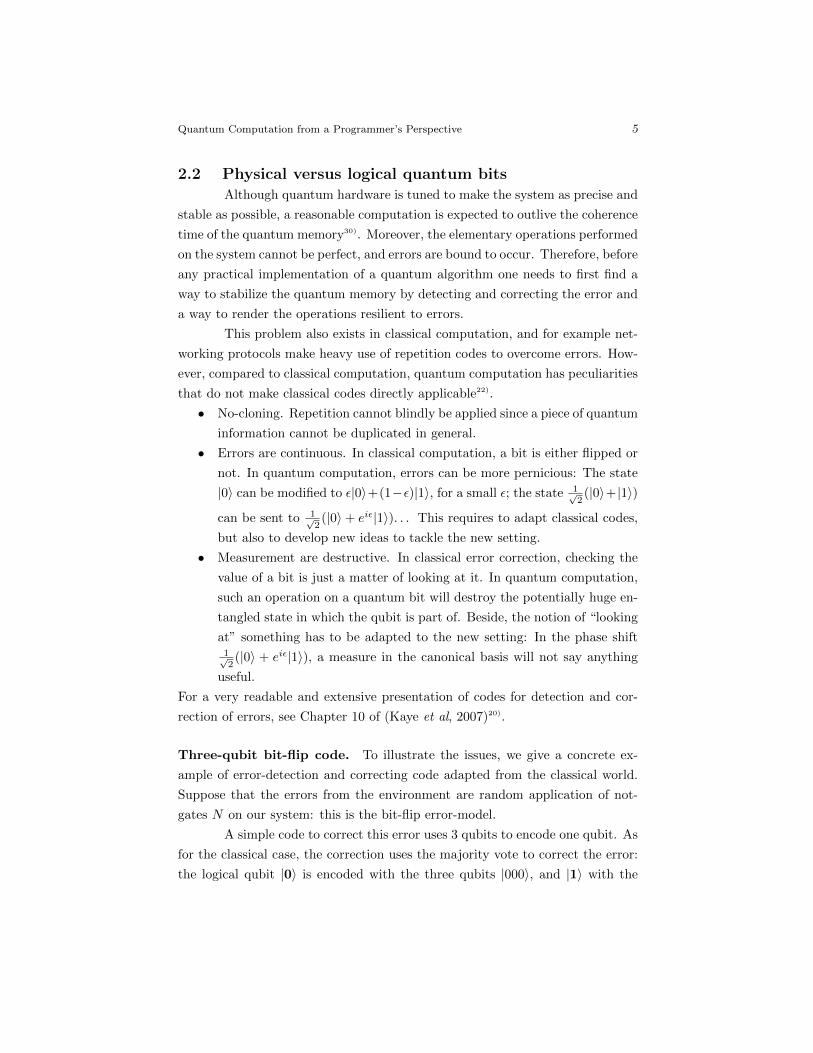
Three-qubit bit-flip code. To illustrate the issues, we give a concrete ex-
ample of error-detection and correcting code adapted from the classical world.
Suppose that the errors from the environment are random application of not-
gates N on our system: this is the bit-flip error-model.
A simple code to correct this error uses 3 qubits to encode one qubit. As
for the classical case, the correction uses the majority vote to correct the error:
the logical qubit |0〉 is encoded with the three qubits |000〉, and |1〉 with the
6 Benoıt Valiron
|φ〉 •|0〉 •|0〉 ⊕ ⊕
(a) Creation
• • U1xy
• U2xy
• U3xy
|0〉 ⊕ ⊕ M x
|0〉 ⊕ ⊕ M y
(b) Correction
H • •
⊕⊕
(c) Unitary
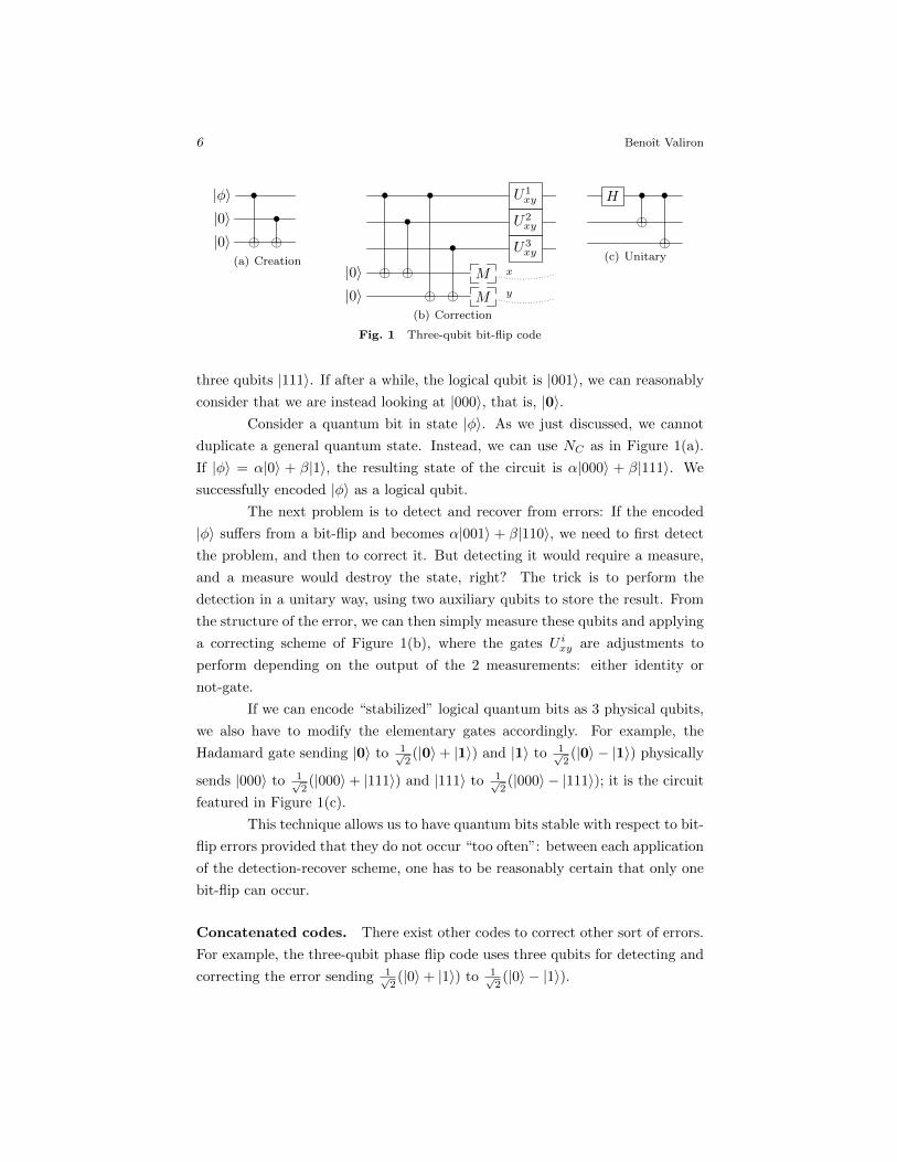
Fig. 1 Three-qubit bit-flip code
three qubits |111〉. If after a while, the logical qubit is |001〉, we can reasonably
consider that we are instead looking at |000〉, that is, |0〉.Consider a quantum bit in state |φ〉. As we just discussed, we cannot
duplicate a general quantum state. Instead, we can use NC as in Figure 1(a).
If |φ〉 = α|0〉 + β|1〉, the resulting state of the circuit is α|000〉 + β|111〉. We
successfully encoded |φ〉 as a logical qubit.
The next problem is to detect and recover from errors: If the encoded
|φ〉 suffers from a bit-flip and becomes α|001〉 + β|110〉, we need to first detect
the problem, and then to correct it. But detecting it would require a measure,
and a measure would destroy the state, right? The trick is to perform the
detection in a unitary way, using two auxiliary qubits to store the result. From
the structure of the error, we can then simply measure these qubits and applying
a correcting scheme of Figure 1(b), where the gates U ixy are adjustments to
perform depending on the output of the 2 measurements: either identity or
not-gate.
If we can encode “stabilized” logical quantum bits as 3 physical qubits,
we also have to modify the elementary gates accordingly. For example, the
Hadamard gate sending |0〉 to 1√2(|0〉+ |1〉) and |1〉 to 1√
2(|0〉 − |1〉) physically
sends |000〉 to 1√2(|000〉+ |111〉) and |111〉 to 1√
2(|000〉 − |111〉); it is the circuit
featured in Figure 1(c).
This technique allows us to have quantum bits stable with respect to bit-
flip errors provided that they do not occur “too often”: between each application
of the detection-recover scheme, one has to be reasonably certain that only one
bit-flip can occur.
Concatenated codes. There exist other codes to correct other sort of errors.
For example, the three-qubit phase flip code uses three qubits for detecting and
correcting the error sending 1√2(|0〉+ |1〉) to 1√
2(|0〉 − |1〉).

Quantum Computation from a Programmer’s Perspective 7
When one has two codes, for example the bit-flip code and the phase-
flip code, it is possible to concatenate them in the sense that the (logical) input
qubit of one code will be the output of the other code. In the case of these
two codes, we get the Shor code, correcting an arbitrary error happening on a
logical quantum bit, by using 9 physical qubits. Although it corrects only one
error at a time, this could be partially solved by concatenating yet another code.
However, even for this simple concatenation, the resulting logical qubit uses 9
physical qubits. And if we were concatenating more codes, the number of qubits
would be even larger.
An increase in the number of quantum bits means more memory man-
agement: more qubits need to be allocated and potentially moved around. Also,
the logical elementary operations are hindered by a corresponding overhead.
Given a particular hardware, there is therefore a subtle analysis to per-
form: sure enough there is some decoherence going on. But if it is possible at
all, what is the cost of a fault-tolerant quantum computation on this hardware?
Does the concatenation of one, two, three codes helps? If it does, it has to
be balanced with the increased number of physical quantum bits and physical
elementary gates required for their logical alter-ego.
For a real quantum computer with several hundreds of logical qubits,
this analysis will probably be daunting to perform by hand only. Dedicated
software analysis tools will be needed for fine tuning the design of a code for a
particular hardware combination. This is one of the place where programming
techniques and analysis might end up useful, if not necessary.
§3 Quantum programmingIn the discussion so far, we only hinted in a few places that formal
language should probably be a good thing for the field of quantum computa-
tion. This section is the place where we really pledge for quantum programming
languages: why we need them (or will soon), what can they bring, and some
guidelines to follow in order to get the best out of them. We then present two
existing languages with some good features but yet some drawbacks, showing
what we find are good directions to follow in the quest for an “ideal” program-
ming language.
3.1 The need for quantum programming languageIf eventually a quantum computer with enough quantum memory is

8 Benoıt Valiron
built, it is worthwhile to wonder how to use it. Several aspects require to be
taken into consideration.
Writing of algorithms. At a high-level view, the algorithms that we de-
scribed in Section 6 (Part 130)) are good examples of informally described al-
gorithms: no parser will ever be able to automatically transform the textual
description into an actual sequence of elementary operations.
There is therefore the need for a reasonably rich language for describing
quantum computation. At a minimum, the language should have the abilities21):
1. to allocate quantum registers, to apply unitaries and to measure quan-
tum registers;
2. to reason about quantum subroutines: to reverse a subroutine and to
condition it over the state of a quantum register;
3. to build a quantum oracle out of the description of a classical function.
Specification and verification. In classical programming languages, debug-
gers are useful tools while writing programs. In quantum computation, due to
impossibility to watch quantum information without modifying it, a debugger
for a program is a lost cause.
In classical programming languages, one can develop test suites to an-
alyze the behavior of a program and check whether it (statistically) behaves
correctly in the expected input data-range. In the case of embedded software, if
it is not possible to do it with the actual device, one can usually perform these
tests off-site. In quantum computation, because of the cost of running code
early quantum computers and the impossibility to efficiently simulate quantum
computation on large inputs, test suites are not an option.
In typed classical programming languages, one has the choice between
strong type systems, dynamic type systems, or even blends of these, bearing the
fact that run-time errors can be captured and potentially resolved by the user
(as in LISP, for example). In quantum computation, due to the cost of the run
of a quantum computation and the difficulty to keep stable quantum memory,
the programmer cannot afford run-time errors in his code, specially if they come
from something as simple as the attempt to clone a quantum bit.
The conclusion is that the work have to be done upstream.
• A program needs to be specified and verified beforehand. A quantum
programming language therefore needs to come up with a well-defined

Quantum Computation from a Programmer’s Perspective 9
and sound semantics, in which one can specify a particular behavior for
a piece of code, and eventually prove that the code behave as expected.
• Because of the cost of each run, the compiler of the programming language
should catch most of the standard causes of run-time errors: the language
needs a strong type system.
Resource sensitivity. At first, quantum computers will probably not have a
very large quantum memory. The programming language should come up with
tools to estimate the resources needed to run a particular piece of code: whether
it is the number of required quantum bits or the number of elementary gates to
be applied.
A particular issue in that respect is the place of the error detection-
correction scheme: should it be managed at the code level, so that the program-
mer can potentially choose which code to use or apply some smart optimization,
should it be left to the compiler, or should it be implemented directly in the
quantum device? A programming language for quantum computation should be
designed in order to be able to deal with codes for error management.
Existing languages for quantum computation. Various quantum pro-
gramming languages have been proposed in the literature14), both imperative-
style and functional-style. Many of these programming languages are theoretical
apparatuses to explore particular aspects of quantum computation and not de-
signed as scalable tools.
First, there is a trend of works developing notations for quantum Turing
machines, one of the paradigms we did not discuss here: its main use is of
theoretical nature.
In the realm of imperative programming languages, it is worthwhile men-
tioning the first real quantum programming language, QCL23), designed by Omer
between 1998 and 2004. This fine piece of software proposes a C-like language
with many nifty features for what he calls “structured quantum programming”.
The result is a language with a relatively natural way of writing algorithms.
However, with respect to the list of requirements we developed for a successful
programming language, QCL fails short in the specification/verification aspect,
and in the ability to address resource sensitivity. Various other imperative lan-
guages follows QCL footsteps. In particular, a C++ extension4) providing a hint
at a compilation process, the command-guarded language qGCL25). . .

10 Benoıt Valiron
In the realm of quantum functional programming, the proposed lan-
guages are usually coming up with a semantics: either denotational, as the
first-order QPL26) and the quantum lambda-calculus described in Section 3.2, or
operational, as van Tonder’s calculus31), or QML2), a purely quantum language
with compilation in term of quantum circuits, or the line of works proposing an
embedded language in Haskell and from which Section 3.3 is derived.
In the following, we discuss two approaches that we feel partially answer
the requirements we discussed in this section, and that might serve as a base for
future approaches: the quantum lambda-calculus of Selinger and Valiron28) and
the Haskell-embedded quantum IO monad of Green and Altenkirch17). Their
interest lies in the fact that despite their shortcomings, they are not only rea-
sonably expressive but also they possess a well-defined and extendable semantics
offering the premises of a specification.
3.2 A toy language for the QRAM modelWe first present a minimal ML-style language for the QRAM model28).
The intuition is the following.
1. The language should be able to express any classical, boolean computa-
tion; it should be higher-order and contain pairing constructs; it should
contain term constructs to express quantum bit creation, unitaries and
measurements.
2. Quantum data should be a first-class citizen: one should be able to
manipulate classical and quantum data with the same term constructs;
variables holding quantum data should be no different from variable
holding classical data; quantum data should be usable at higher-order.
3. The language should be typed and verify usual safety properties, plus
the additional requirement that it should forbid non-duplicable data to
be duplicated.
4. The only side-effect should come from the probabilistic measurement.
In particular, one should not need particular type constructors to hold
quantum data.
The language is formally defined as a lambda-calculus. A lambda-term
is an expression made of the following core grammar, written in BNF form:
Term M,N,P ::= x |MN | λx.M | ifM then N else P | 0 | 1 | ∗ |meas | new | U | 〈M,N〉 | let 〈x, y〉 = M in N,

Quantum Computation from a Programmer’s Perspective 11
where x ranges over an infinite set of term variables and U a set of unitary
gates; the term ifM then N else P stands for a test on P with output M if true,
N else; the constant terms 0 and 1 stand for the boolean values false and true
respectively; ∗ is the result of a command; the constant terms meas, new and
U stand respectively for the measurement, the creation and the application of
a unitary gate on a quantum bit; the terms let 〈x, y〉 = M in N stands for the
retrieval of the content of a pair.
We identify terms up to α-equivalence, defined as usual3). Similarly, the
notions of free and bound variables and of substitution are standard. We use
syntactic sugar for programs when the context is clear: let x = M in N for
(λx.N)M , and λ〈x, y〉.M for λz.(let 〈x, y〉 = z in N).
This language is purely functional: for example, a fair coin can be im-
plemented as the term meas(H(new 0)), where H is the Hadamard gate.
[3.2.1] Abstract machine
Although we want the language to perform quantum computation, no
quantum bit was added into the terms of the language. For example we might
want to represent the constant function outputting a quantum bit, as λx.(α|0〉+β|1〉). The reason why we do not allow such a notation is the problem of entan-
glement. As discussed in the first article of this series30), it is not always possible
to write a two quantum bit system in the form |φ〉 ⊗ |ψ〉. Therefore, if x is the
variable corresponding to the first quantum bit and y the one corresponding to
the second in an entangled state, it is not possible to write classically the term
(λf.fx)(λt.(gy)t) as there is no means of writing x and y.
This non-local nature of quantum information forces us to introduce a
level of indirection for representing the state of a quantum program. Following
the scheme of the QRAM model, we describe an abstract machine consisting of
a lambda-term M , an array of quantum bits Q (the QRAM), and a map linking
variables in M to quantum bits in Q. Formally, an abstract machine is a triple
[Q,L,M ], where
• Q is a normalized vector of ⊗ni=1C2, for some n > 0, called the quantum
array.
• M is a lambda term,
• L is an injective function from a set |L| of term variables to 1, . . . , n,where FV (M) ⊆ |L|. L is called the linking function.
We write |Q| = n. If L(xi) = i, we will sometimes write L as the ordered list

12 Benoıt Valiron
|x1 · · ·xn〉. The idea is that the variable xi is bound in the term M to qubit
number L(xi) of the state Q. We also call the pair (Q,L) a quantum context.
If there are no quantum bits, i.e. if Q ∈ C, we write Q = |〉. Similarly, if L is
empty we write L = |〉.
[3.2.2] Evaluation Strategy
Although we solved the problem of entanglement, there is another issue
that prevents us from blindly using substitution, namely the probabilistic nature
of the measurement: since tossing a coin and duplicating the result is not the
same thing as duplicating the coin and tossing each instance, we need to make
a choice of reduction strategy.
A reduction strategy is a deterministic procedure for reducing a general
abstract machine to a result. There are two main reduction strategies for the
lambda-calculus: in the presence of (λx.M)N , either we blindly substitute N
for x in M : this is call-by-name; or we first reduce N to a result before doing
the substitution: this is call-by-value.
In quantum computation, because of the non-duplicability of a quantum
bit, the choice of reduction strategy might even render invalid a piece of code.
For example, if x links to a quantum bit, the code (λfx.(fx)x)(meas x) cannot
be reduced right ahead to λf.(f((meas x))((meas x) as this duplicate the quan-
tum bit. We first have to apply the measure, yielding a classical bit that can
effectively be duplicated.
Generally speaking, in call-by-name a measurement of the form measM
is carried over along β-reductions. There is no possible way to “force” the
measurement to happen. However, it is possible to simulate a call-by-name
reduction in call-by-value by encapsulating terms in lambda-abstractions. For
example, to carry over the term measM using a call-by-value reduction strategy,
one can write the term as λy.measM , with y a fresh variable.
Because of this flexibility, in this quantum lambda-calculus we consider
the call-by-value reduction strategy.
[3.2.3] Reduction rules
We then define a probabilistic call-by-value reduction procedure for the
quantum lambda calculus. Note that, although the reduction itself is probabilis-
tic, the choice of which redex to reduce at each step is deterministic.

Quantum Computation from a Programmer’s Perspective 13
[ Q,L, if 0 then M else N ]→1 [ Q,L,N ]
[ Q,L, if 1 then M else N ]→1 [ Q,L,M ]
[ Q,L,U〈xj1 , . . . , xjn〉 ]→1 [ Q′, L, 〈xj1 , . . . , xjn〉 ]
[ α|Q0〉+ β|Q1〉, L,meas xi ]→|α|2 [ |Q0〉, L, 0 ]
[ α|Q0〉+ β|Q1〉, L,meas xi ]→|β|2 [ |Q1〉, L, 1 ]
[ Q, |x1 . . . xn〉,new 0 ]→1 [ Q⊗ |0〉, |x1 . . . xn+1〉, xn+1 ]
[ Q, |x1 . . . xn〉,new 1 ]→1 [ Q⊗ |1〉, |x1 . . . xn+1〉, xn+1 ]
Table 1 Reductions rules of the quantum lambda calculus
A value is a term of the following form:
Value V,W ::= x | λx.M | 0 | 1 | ∗ | meas | new | U | 〈V,W 〉.
An abstract machine of the form [Q,L, V ] where V is a value is called a quantum
value-state.
The reduction rules are shown in Table 1. We write [Q,L,M ] →p
[Q′, L′,M ′] for a single-step reduction of states which takes place with prob-
ability p. In the rule for reducing the term U〈xj1 , . . . , xjn〉, U is an n-ary
built-in unitary gate, j1, . . . , jn are pairwise distinct, and Q′ is the quantum
state obtained from Q by applying this gate to qubits j1, . . . , jn. In the rule for
measurement, |Q0〉 and |Q1〉 are normalized states of the form
|Q0〉 =∑j
αj |φ0j 〉 ⊗ |0〉 ⊗ |ψ0
j 〉, |Q1〉 =∑j
βj |φ1j 〉 ⊗ |1〉 ⊗ |ψ1
j 〉,
where φ0j and φ1
j are i-qubit states (so that the measured qubit is the one pointed
to by xi). In the rule for new , Q is an n-qubit state, so that Q⊗|i〉 is an (n+1)-
qubit state.
There are also ξ-rules for each term constructor, such as
[ Q,N ]→p [ Q′L, ,N ′ ]
[ Q,L,MN ]→p [ Q′, L,MN ′ ]
[ Q,M ]→p [ Q′, L,M ′ ]
[ Q,L,MV ]→p [ Q′, L,M ′V ]
or
[ Q,L, P ]→p [ Q′, L, P ′ ]
[ Q,L, if P then M else N ]→p [ Q′, L, if P ′ then M else N ]
keeping in mind that we do not reduce under the branches of a test.
[3.2.4] Type System

14 Benoıt Valiron
The reduction system has run-time errors: the state [Q,L,H(λx.x)] and
the state [Q, |xyz〉, U〈x, x〉] are both invalid. In the next section, we introduce
a type system designed to rule out such erroneous states.
Types In the lambda calculus we just defined, we need to be able to account
for higher-order, products, classical booleans and quantum booleans. Since we
do not want to have specific term constructs for dealing with duplication and
non-duplication, the information has to be encoded into the type system. We
use a type system inspired from linear logic15). By default, a term of type A
is assumed to be non-duplicable, and duplicable terms are given the type !A
instead.
Formally, we define the following type system for the quantum lambda
calculus as follows:
qType A,B ::= bit | qbit | !A | (A(B) | > | (A⊗B).
The constant types bit and qbit stand respectively for the classical and the
quantum booleans; the type !A is for duplicable elements of type A; the type
A(B for functions from A to B; the type > for result of commands; the type
A⊗B for pairs of elements of types A and B.
We call the operator “!” the exponential.
The typing rules will ensure that any value of type !A is duplicable.
However, there is no harm in using it only once; thus, such a value should also
have type A. For that purpose, we use a subtyping relation to capture this
notion: the subtyping is morally stating that !A <: A, and verifying the usual
properties otherwise: A ⊗ B <: A′ ⊗ B′ and A′( B <: A( B′ provided that
A<:A′ and B <:B′.
Typing Rules A typing judgment is the given of a set ∆ = x1 : A1, . . . , xn :
An of typed variables, a term M and a type B, written as ∆ BM : B. We call
the set ∆ the typing context, or simply the context.
Given two contexts ∆1 and ∆2, we write (∆1,∆2) for the context con-
sisting of the variables in ∆1 and in ∆2. When described in this form, it is
assumed that |∆1| ∩ |∆2| = ∅.A typing derivation is called valid if it can be inferred from the rules
of Table 2. We write !∆ for a context of the form x1 : !A1, . . . , xn : !An.We use the notation |∆| to represent the set of (untyped) variables x1, . . . , xn

Quantum Computation from a Programmer’s Perspective 15
contained in ∆. In the table, the symbol c spans the set of term constants
meas,new , U, 0, 1. To each constant c we associate a term Ac, as follows:
A0, A1 = bit , Anew = bit ( qbit , AU = qbit⊗n ( qbit⊗n, Ameas = qbit ( !bit .
The type !Ac is understood as being the “most generic” one for c, as
enforced by the typing rule (ax 2). For example, we defined Anew to be bit(qbit .
Since new can take any type B such that !Ac <:B, the term new can be typed
with all the types in the poset:
!(!bit ( qbit)<:
!(bit ( qbit)<:
<:!bit ( qbit .
bit ( qbit<:
This implies, as expected, that no created quantum bit can have the type !qbit .
In general, the type system enforces the requirement that variables hold-
ing quantum data cannot be freely duplicated; thus λx.〈x, x〉 is not a valid term
of type qbit(qbit⊗qbit . On the other hand, we allow variables to be discarded
freely.
Note also that due to rule (λ2) the term λx.M is duplicable only if all
the free variables of M (other that x) are duplicable. This follows the call-by-
value approach: since λx.M is a value, if it is duplicated it will be duplicated
as a syntactic string of symbols, thus duplicating every single free variable of it
(other than x).
Properties of the Type System An abstract machine [ Q,L,M ] can be
said to be well-typed (or valid) of type A as one could expect: M needs to be of
type A, and all the variables in L are taken to be of type qbit .
The properties of the type system are then canonical: A well-typed
program only reduces to well-typed programs of the same type, and if a program
is well-typed, either it is a value or it reduces to some other program.
[3.2.5] Example: quantum teleportation
It turns out that some quantum algorithms can be efficiently understood
as elements of higher-order types. We give in this section the implementation
of the teleportation procedure as a higher-order term, despite the fact that the
usual formalism is completely sequential30).
The Teleportation Procedure Consider the teleportation algorithm as it is
described in Section 4.3 (Part 130)). We can embed each part of the procedure
16 Benoıt Valiron
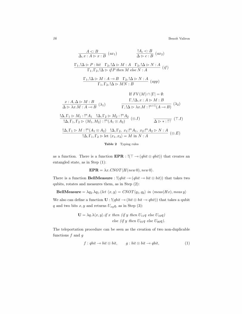
A<:B∆, x : A B x : B
(ax 1)!Ac <:B
∆ B c : B(ax 2)
Γ1, !∆ B P : bit Γ2, !∆ BM : A Γ2, !∆ B N : A
Γ1,Γ2, !∆ B if P then M else N : A(if )
Γ1, !∆ BM : A(B Γ2, !∆ B N : A
Γ1,Γ2, !∆ BMN : B(app)
x : A,∆ BM : B
∆ B λx.M : A(B(λ1)
If FV (M) ∩ |Γ| = ∅:Γ, !∆, x : A BM : B
Γ, !∆ B λx.M : !n+1(A(B)(λ2)
!∆,Γ1 BM1 : !nA1 !∆,Γ2 BM2 : !nA2
!∆,Γ1,Γ2 B 〈M1,M2〉 : !n(A1 ⊗A2)(⊗.I)
∆ B ∗ : !> (>.I)
!∆,Γ1 BM : !n(A1 ⊗A2) !∆,Γ2, x1:!nA1, x2:!nA2 B N : A
!∆,Γ1,Γ2 B let 〈x1, x2〉 = M in N : A(⊗.E)
Table 2 Typing rules
as a function. There is a function EPR : !(>( (qbit ⊗ qbit)) that creates an
entangled state, as in Step (1):
EPR = λx.CNOT 〈H(new 0),new 0〉.
There is a function BellMeasure : !(qbit ( (qbit ( bit ⊗ bit)) that takes two
qubits, rotates and measures them, as in Step (2):
BellMeasure = λq2.λq1.(let 〈x, y〉 = CNOT 〈q1, q2〉 in 〈meas(Hx),meas y〉
We also can define a function U : !(qbit ( (bit ⊗ bit ( qbit)) that takes a qubit
q and two bits x, y and returns Uxyq, as in Step (3):
U = λq.λ〈x, y〉.if x then (if y then U11q else U10q)
else (if y then U01q else U00q).
The teleportation procedure can be seen as the creation of two non-duplicable
functions f and g
f : qbit ( bit ⊗ bit , g : bit ⊗ bit ( qbit , (1)
Quantum Computation from a Programmer’s Perspective 17
such that (g f)(x) = x for an arbitrary qubit x. We can construct such a pair
of functions by the following code:
let 〈x, y〉 = EPR ∗ inlet f = BellMeasure x in
let g = U y
in 〈f, g〉.
Note that, since f and g depend on the state of the qubits x and y, respectively,
these functions cannot be duplicated, which is reflected in the fact that the types
of f and g do not contain a top-level “!”.
[3.2.6] Shortcomings of the language
This quantum lambda-calculus provides a sound and unified framework
for manipulating classical and quantum data. It also makes it possible to po-
tentially define oracles as higher-order functions. The language successfully ad-
dresses the issue of the distinction between duplicable and non-duplicable data,
even at higher-order type, and do so in a general manner. Finally, it can easily
be extended with a richer type system (such as lists) and recursion29).
However, it has several shortcomings that cannot be overcome with a
simple extension: first, if it is possible to write and manipulate oracles as first-
class objects, there is no way to automatically make a unitary map out of a
classical description: the only unitaries around are the elementary ones. It
also lacks a way of manipulating quantum circuits. For example, one cannot
reverse a computation. It is not possible to process a quantum circuit to remove
redundancies, or describe and apply optimization. It is neither possible to apply
an error correcting code to a given function within the language.
3.3 A toy language for circuit constructionThe shortcomings described in Section 3.2.6 are mainly due to the fact
that the semantics of the quantum lambda-calculus does not separate circuit
construction from circuit evaluation. The quantum IO monad of Green and
Altenkirch17) proposes an alternative approach for dealing with quantum com-
putation, and the technique addresses this particular problem.
The language follows an intuition different from the one developed in
the quantum lambda-calculus.
1. First, the language is a language embedded in a host language, Haskell.

18 Benoıt Valiron
The choice of the host language has its importance: Haskell is a higher-
order, functional language with a rich type system (much richer than
the ML type-system, for example). This makes it a good candidate for
hosting an embedded language while giving it a well-defined operational
semantics.
2. The language separates the construction of a quantum computation
from its execution. While being built, the computation is stored in a
datastructure that one could then theoretically manipulate. As such,
the language only proposes commands to run various simulations, but
the implementation is modular enough to imagine being able to add
a “run” command to hook on a real quantum computer, or add some
commands to perform code rewriting.
3. The other noteworthy feature of the quantum IO monad is the use of
Haskell’s rich type system to define a notion of generic quantum data.
With a single term construct, one can define the measure of a tuples of
quantum bits, or a list of quantum bits, or a tuples of list of quantum
bits. . . This gives a concrete definition of the otherwise vaporous notion
of quantum data.
In the following, we give a brief tutorial to the quantum IO monad, illustrating
the features that are worth having in a quantum programming language. Al-
though the language being embedded in Haskell, we’ll try our best to make the
exposition self-contained. Haskell code is written in typewriter font.
[3.3.1] An embedded language in Haskell
Standing on top of Haskell, the language comes with three main specific
type constructors: a type of quantum bits Qbit, a type of unitary maps U, and
a type constructor for quantum computation QIO. A function of type A→ QIO B
is understood as a function from an object of type A, returning a quantum
computation whose result would be of type B. The type constructor QIO records
the fact that some non-purely functional operations are taking place along the
evaluation of the function.
Elementary quantum computation. The basic blocks of quantum compu-
tation are represented as Haskell functions.
• measQbit :: Qbit -> QIO Bool. For measurements: a function taking
a qubit as input and outputting a classical boolean.

Quantum Computation from a Programmer’s Perspective 19
• mkQbit :: Bool -> QIO Qbit. For creating quantum bits: a function
taking a classical boolean as input and producing a quantum bit.
• applyU :: U -> QIO (). For unitaries: it is a command taking a uni-
tary matrix as input, and producing. . . a quantum computation. A
command is a function of output type void, represented by the empty
tuple () in Haskell.
Building unitaries. How are we to build unitaries of type U? The following
operations are at available.
• swap :: Qbit -> Qbit -> U. For swapping the quantum bits refer-
enced by the two inputs.
• cond :: Qbit -> (Bool -> U) -> U. For dynamically constructing of
controlled operation. This operation is nothing else than an if-then-else
construction for quantum bit, as it was already proposed in QML2).
• rot :: Qbit -> ((Bool,Bool) -> C) -> U. The first input is a ref-
erence to a quantum bit, and the second input is the description of a 2×2
matrix. This operation constructs the circuit applying the matrix to the
qubit.
• ulet :: Bool -> (Qbit -> U) -> U. Allocation of auxiliary ancillas.
First the ancilla is created with the value of the first input, then the
second argument is applied to this ancilla. Finally, the ancilla is erased
(i.e. measured).
• urev :: U -> U. Reverse the circuit description given in input.
Finally, the type U is enriched with the notion of monoid (thanks to Haskell’s
typeclass Monoid). Practically, this means that two other useful constructions
are available: mempty :: U, representing the empty circuit and mappend ::
U -> U -> U, representing sequencial composition of circuits.
Example of unitary constructions. The Hadamard gate, using an auxil-
liary function:
hadMat :: (Bool,Bool) → ChadMat (True,True) = -0.707...
hadMat (_,_) = 0.707...
uhad :: Qbit → U
uhad q = rot q hadMat
20 Benoıt Valiron
One can define a generic control operator as a one-sided if-construction:
ifQ :: Qbit → U → U
ifQ q u = cond q (λx → if x then u else mempty)
Using lists of quantum bits (in Haskell, [A] is the notation for a list of elements
of type A), one can use the programmable feature of the circuit construction and
define a multi-control operation with recursion.
ifQx :: [Qbit] → U → U
ifQx [] u = u
ifQx (h:t) u = ifQ h (ifQx t u)
Arguably, this program is implementing a multi-controlled gate in a “natural”
way.
General quantum computation. Haskell proposes an imperative style way
for composing operations of type QIO (thanks to the monadic interface). Con-
sider the two functions f :: A → QIO B and g :: B → QIO C. The com-
position of f and g is done using the syntax
h :: A → QIO C
h x = do y <- f x; z <- g y; return z
The syntax is self explanatory: store the result of f x in y, feed it to g, get
z, finally return z. One can of course compose many operations in one go, or
apply commands of type QIO (), extending the syntax in the obvious way. For
example, the coin-toss can be defined as follows.
coinToss :: QIO Bool
coinToss = do
q <- mkQbit False;
applyU (uhad q);
r <- measQbit q;
return r
Quantum teleportation. As a complete example, we show the implemen-
tation of the quantum teleportation algorithm17). Compared to the quantum
lambda-calculus, the main differences is that every function returns a computa-
tion QIO. We assume that unot is the gate N and that uZ is the gate Z.
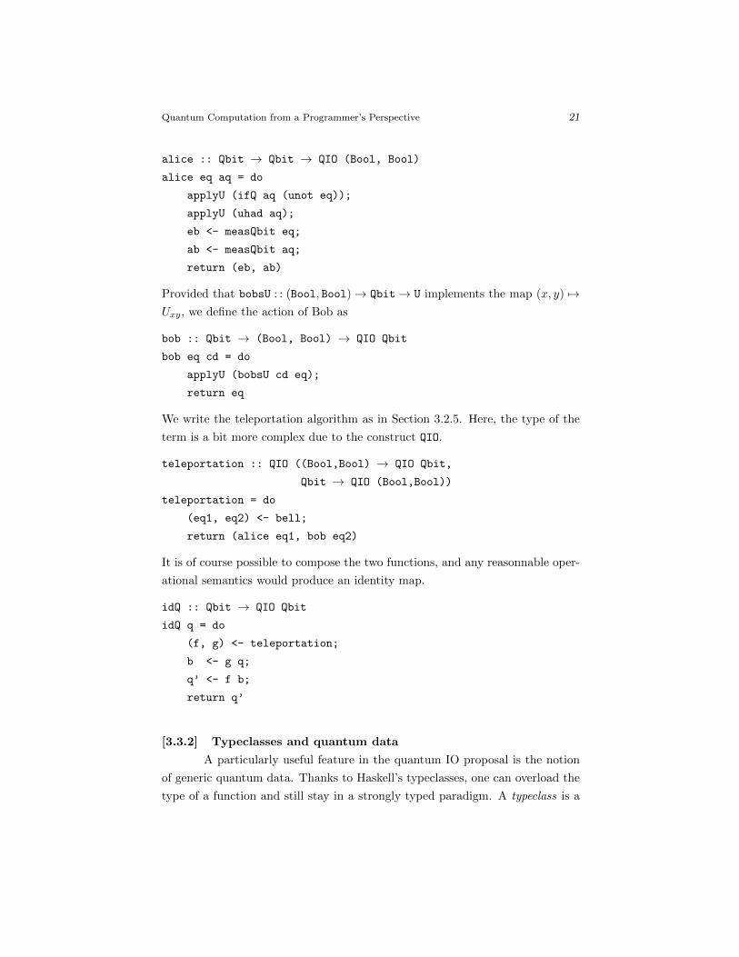
Quantum Computation from a Programmer’s Perspective 21
alice :: Qbit → Qbit → QIO (Bool, Bool)
alice eq aq = do
applyU (ifQ aq (unot eq));
applyU (uhad aq);
eb <- measQbit eq;
ab <- measQbit aq;
return (eb, ab)
Provided that bobsU : : (Bool, Bool)→ Qbit→ U implements the map (x, y) 7→Uxy, we define the action of Bob as
bob :: Qbit → (Bool, Bool) → QIO Qbit
bob eq cd = do
applyU (bobsU cd eq);
return eq
We write the teleportation algorithm as in Section 3.2.5. Here, the type of the
term is a bit more complex due to the construct QIO.
teleportation :: QIO ((Bool,Bool) → QIO Qbit,
Qbit → QIO (Bool,Bool))
teleportation = do
(eq1, eq2) <- bell;
return (alice eq1, bob eq2)
It is of course possible to compose the two functions, and any reasonnable oper-
ational semantics would produce an identity map.
idQ :: Qbit → QIO Qbit
idQ q = do
(f, g) <- teleportation;
b <- g q;
q’ <- f b;
return q’
[3.3.2] Typeclasses and quantum data
A particularly useful feature in the quantum IO proposal is the notion
of generic quantum data. Thanks to Haskell’s typeclasses, one can overload the
type of a function and still stay in a strongly typed paradigm. A typeclass is a

22 Benoıt Valiron
property of a type to which is attached a set of functions. In the case of quantum
data, the quantum IO monad proposes
class Qdata a qa | a -> qa, qa -> a where
mkQ :: a -> QIO qa
measQ :: qa -> QIO a
condQ :: qa -> (a -> U) -> U
That is, the typeclass Qdata place in relation two types a and qa, and define
for each pair (a,qa) three functions mkQ, measQ and condQ. The names of these
functions are deliberately close to the maps mkQbit, measQ and cond, since the
first pair (a,qa) is (Bool,Qbit):
instance Qdata Bool Qbit where
mkQ = mkQbit
measQ = measQbit
condQ = cond
Provided that (a,qa) and (b,qb) are already member of Qdata, we can also
make ((a,b),(qa,qb)) member of Qdata:
instance (Qdata a qa, Qdata b qb) => Qdata (a,b) (qa,qb) where
mkQ (x,y) = (mkQ x, mkQ y)
measQ (x,y) = (measQ x, measQ y)
condQ (x,y) f = condQ x λz → condQ y λz’ → f (z,z’)
Similarly, it is possible to add tuples, and lists in the scheme. But one
can make more “interesting” correspondences; for example, if we define the type
data QInt = QInt [Qbit]
one can make (Int, QInt) into an instance of Qdata (by fixing the number of
digits a QInt is allowed to have, and by choosing whether we are little or big
endian), so that mkQ 4 for example builds the state | . . . 0100〉
[3.3.3] Discussion
The quantum IO monad offers a versatile way of manipulating pieces of
quantum algorithms: quantum circuits on one hand, and quantum computation
in general on another hand. It also features a systematic procedure to extend
quantum datatypes. These ideas are to keep in mind while designing a scalable
quantum programming language.

Quantum Computation from a Programmer’s Perspective 23
However, several drawbacks hamper the language, and does not make it
the perfect fit we were looking for.
1. The type of unitaries U is untyped. As such, a unitary is a blackbox
that does not contain any information on the structure of the input
and the output. Unitaries cannot easily be used with Qdata.
2. The typeclass Qdata leaves the programmer frustrated: the correspon-
dence classical-quantum is only drawn for elementary functions: how
about producing a map QInt → QInt out of a map Int → Int?
3. Despite its power, Haskell’s type system is not capable of forbidding
duplication of quantum bits. For example, the following buggy code is
nonetheless valid:
copy :: Qbit -> QIO (Qbit, Qbit)
copy q = do return (q,q)
This is certainly problematic in the light of our requirements for a
quantum programming language.
3.4 Monads and quantum computationAlbeit kept under the shed, in the two languages we reviewed a struc-
turing notion kept showing up: the notion of monad. Monads are semantic tools
to capture and reason about side-effects.
Side-effects appear in a language when the notion of value, or result is
distinct from the notion of computation. Exemples of side-effects include.
• Probabilistic behavior. If there is a way to toss a coin in a language, the
coin-toss is operationally distinct from its result.
• Input-output. If the language possesses a library for accessing a terminal,
or a tape, or a network, or a file-system. . . , sure enough a computation
is not similar to a result.
• State. If references, or pointers are available in the language, this can
often be represented by a monad.
These three side-effects appear in the situations we explored:
• QIO is can be regarded as input-output,
• U is a state monad,
• the measurement induces a probabilistic side-effect.

24 Benoıt Valiron
In the quantum lambda-calculus, the operational semantics makes use of an ex-
plicit state monad to keep track of the quantum bits already allocated. However,
thanks to the type system enforcing linearity on quantum bits, a computation
involving unitaries (such as H (N x)) is the same thing as the result of the com-
putation (since one can only use it once): in the quantum lambda-calculus, the
quantum bits is not the part breaking the pure functionality of the language.
The important aspects these two languages teach us is that
• linear type systems can efficiently deal with the non-duplicability of quan-
tum information;
• monads are probably the good paradigm to manipulate quantum circuits
and quantum computation as a piece of data.
• generic quantum data definable by the programmer makes sense, but
should be used in parallel with automatic classical-to-quantum conversion
to take full advantage of their genericity.
3.5 Semantics of quantum computationA second research area is the development of semantics for quantum
computation. The goal is two-fold. First, understanding the structure of quan-
tum information13). Then, developping tools for specification and verification
of quantum algorithms. In the event of quantum computers, these tools might
reveal as useful as they were for classical computation32).
[3.5.1] Completely positive maps
A well-known fact22) is that vectors in Hilbert spaces do not form a
satisfying framework to describe quantum computation when it involves mea-
surement. Consider the two computations
new (meas (H (new 0))), (2)
H (new (meas (H (new 0))). (3)
The former outputs the equal probability distribution consisting of the states |0〉and |1〉 whereas the latter outputs the equal probability distribution consisting of
the states 1√2(|0〉+ |1〉) and 1√
2(|0〉− |1〉). One can argue that these are distinct.
However, this is not the case: there are observationally equivalent, i.e. one
cannot find a computation that can distinguish between them. For example, if
you simply measure them with respect to the standard basis, they both answer 0
and 1 with equal probability. Intuitively, the idea is that a quantum computation

Quantum Computation from a Programmer’s Perspective 25
on either state is morally “just” a general measurement, and one can generalize
this idea to build a denotational semantics for quantum computation.
A representation that is invariant under this observational equivalence is
the notion of positive matrix. There are several equivalent definitions for positive
matrices. The one of interest in our situation is this one:
Definition 3.1
A positive matrix is a square-matrix of the form∑ni=1 ρiuiu
∗i where the ρi’s
are non-negative reals, the ui’s are normalized vectors of same dimension. The
notation u∗i represents the conjugate transpose of ui. That is, if ui is the 2-
dimensional vector ( αβ ), u∗i is the row-vector (α β). The element uiu∗i is then
the 2× 2 matrix ( αα αββα ββ
).
One can therefore represent a probabilistic superposition of states by
taking the ρi’s as the probability for a particular state ui to be the result of the
computation. Then in the above example, the output of Program (2) is
1
2
(1
0
)(1 0) +
1
2
(0
1
)(0 1) =
(12 0
0 12
),
whereas the output of Program (3) is
1
2
(1√2
1√2
)( 1√
21√2) +
1
2
(1√2
-1√2
)( 1√
2-1√
2) =
1
2
(12
12
12
12
)+
1
2
(12
-12
-12
12
)=
(12 0
0 12
).
Their representation in term of positive matrices is the same: this is consistent
with the fact that the two programs are indistinguishable.
If the result of a computation is a positive matrix, a computation is a
completely positive map. That is:
• sending positive matrices to positive matrices;
• linear, in the sense of linear algebra: if the map is f , f(x+y) = f(x)+f(y)
and f(ρ · x) = ρ · f(x).
If we deal with first-order maps (i.e. with inputs and outputs being only classical
and quantum bits), one can also add
• trace-preserving,
in which case the map is called a superoperator.
Denotational semantics. A denotational semantics for a programming lan-
guage is a mathematical representation of its programs. A program is regarded

26 Benoıt Valiron
as a process inputting some data and outputting some other data: its semantics
is a function whose domain is the datatype of input and whose codomain is the
datatype of output.
The semantics of a programming language can have three properties: ad-
equacy, full-abstraction and full completeness. If [[P ]] represents the denotation
of the program P , we can define these notions as follows32).
• Let Ω be the diverging program. The semantics is adequate if when-
ever [[P ]] = [[Ω]] where Ω is the looping program, then P is also non-
terminating.
• The semantics is fully-abstract if for all programs P and Q, [[P ]] = [[Q]] if
and only if P and Q are observationally equivalent. A potential use for a
fully abstract semantics is to validate code optimization, for example in
the context of the construction of a compiler.
• Finally, the semantics is fully complete if moreover, every element v in the
image of a type A corresponds to a program P . With such a semantics,
one has a decision tool that can determine using mathematical methods
whether a given set of specifications can be realized by a program.
Quantum lambda-calculus. Positive matrices and completely positive maps
form a denotational for the quantum lambda-calculus in the following sense.
• Completely positive maps form a fully-abstract semantics for the strictly
linear fragment of the quantum lambda-calculus27): the model only rep-
resents programs whose types do not contain any instance of “!”. In
particular, if f and g are the two functions built in Section 3.2.5, then
g f : qbit → qbit has the same denotation as the identity function λx.x.
• Superoperators form a complete semantics for the first-order fragment of
the stricly linear lambda-calculus26). This means that any superoperator
can be regarded as a program unique up to observational equivalence,
and vice-versa.
[3.5.2] Linear logic
Completely positive maps does not capture the whole quantum lambda-
calculus: duplication is not handled. One can wonder what is the structure of
the type operator “!”, and what are the properties it satisfies.
Programs and Proofs. Through the Curry-Howard correspondence19), the
type of a program can be interpreted as a proposition in a particular logic. The

Quantum Computation from a Programmer’s Perspective 27
program corresponds to the proof of the proposition, and the cut-elimination
of the proof corresponds to the evaluation of the program. A rich enough logic
admits a notion of conjunction ∧ and a notion of implication ⇒. In the type
system, these correspond to pairing and function types. In the realm of the
semantics, the connectives (∧,⇒) forms an adjunction, a powerful categorical
notion.
The notions of semantics, typed languages and logical systems interact
in complex ways, each one giving insight on the structure of the other ones.
A modality for non-linearity. Linear logic is a resource-sensitive logic in-
troduced by Girard15). This logic acknowledges the fact that the structural rules
are usually hidden in regular, classical logic: for example, the introduction rule
for the conjunction can be decomposed in two distinct ways, giving rise to two
distinct conjunctions: a multiplicative ⊗ and an additive &:
∆ B A Γ B B∆,Γ B A⊗B
∆ B A ∆ B B∆ B A&B
In order to go from one to the other, one needs to apply two structural rules:
weakening and contraction:
A B CA,B B C
A,A B B
A B B
In linear logic, structural rules can only be applied on formulas of the form !A.
In general there are four structural rules: weakening and contraction, but also
dereliction and promotion, respectively:
A B CA, !B B C,
!A, !A B B
!A B B ,A B B!A B B,
!A B B!A B!B.
The modality “!” can be regarded as the duplicability flag in the type system
of the quantum lambda-calculus: weakening and promotion restricts which data
can be erased and duplicated, whereas derelication and promotion relate dupli-
cable data with non-duplicable data.
A valid typing judgement in the quantum lambda-calculus can therefore
be seen as a proof in a linear-logic-like logical system. It does not match precisely
linear logic because the type operator “!” is weaker: in particular, !!A is a type
equivalent to !A, which is not the case in linear logic.

28 Benoıt Valiron
Relation with models. If the two logical systems do not match precisely,
they match enough to be able to adapt models of linear logic to the subset of
quantum computation described by the quantum lambda-calculus. Specically,
many models of linear logic are based on functional analysis and theory of opera-
tor spaces, and use the algebraic linearity to reflect the logical linearity10, 5, 12, 11).
The spaces used for the models are rich enough to be able to generate the modal-
ities “!” with the correct behavior. It has been shown that in some context it is
possible to use the constructions to make models of quantum computation16, 18).
[3.5.3] Graphs and MBQC
An successful alternative approach to verify properties of quantum pro-
grams is the use of rewriting rules in graphical representation of symmetric
monoidal and compact closed categories. Although this is particularly relevant
in the paradigm of measurement-based quantum computation, it is a tool to
keep an eye on when concerned with optimization of quantum circuits.
Categorical representation. Entanglement structures such as the one de-
signed at the beginning of a computation in the MBQC model (Section 2.1) can
be regarded simply as a graph: called graph state, they possess many properties
that can be abstracted away and described in categorical models9).
The canonical categorical models that can be used to described quantum
computation are the compact closed structures1): for our purpose, their most
interesting aspect is that they feature a graphical language, and equations in
compact closed structures can be set in correspondence with rewrite rules in the
graphical language.
Playing with additional structures on compact closed categories allows
one to describe with sharp precision many constructions in quantum computa-
tion, in particular with what can be done with graph states. A partially au-
tomated tool, Quantomatic8), have been developped for helping the reasonning
in this theoretical framework. It is readily available to help analyzing circuit
optimizations.
§4 ConclusionQuantum computation is yet at an early stage: there does not yet ex-
ist a technology to build scalable quantum computers, and the development is
hindered by the unstability of quantum information.

Quantum Computation from a Programmer’s Perspective 29
However, if the technology is not yet up to scale, the theory behind
quantum computation is well-understood. This is calling for a theoretical com-
puter science to be developed, using all the insight computer science have been
developing for classical computation. Semantical tools are getting shaped: it is
time to develop quantum programming languages and analysis techniques to get
ready for the birth of scalable quantum computers.
This is an exciting field with many open questions and extremely diverse
problematics. We hope this review raised some interest among the readers: this
computational paradigm is still vastly unexplored, and it is calling for expertize
from all domains of computer science.
References
1) Abramsky, S. and Coecke, B., “A categorical semantics of quantum protocols,”in Proc. of LICS’04, pp. 415–425, 2004.
2) Altenkirch, T. and Grattage, J., “A functional quantum programming lan-guage,” in Proc. of LICS’05, pp. 249–258, 2005.
3) Barendregt, H. P., The Lambda-Calculus, its Syntax and Semantics, NorthHolland, 1984.
4) Bettelli, S., Calarco, T. and Serafini, L., “Toward an architecture for quantumprogramming,” The European Physical Journal D, 25, 2, pp. 181–200, 2003.
5) Blute, R. F., Cockett, J. R. B. and Seely, R. A. G., “Differential categories,”Math. Struct. in Comp. Sc., 16, 6, pp. 1049–1083, 2006.
6) Broadbent, A. and Kashefi, E., “Parallelizing quantum circuits,” Th. Comp.Sc., 410, 26, pp. 2489–2510, 2009.
7) Danos, V., Kashefi, E., Panangaden, P. and Perdrix, S., “Extended measure-
ment calculus,” Ch. 713), pp. 235–310.
8) Dixon, L. and Duncan, R., “Graphical reasoning in compact closed categoriesfor quantum computation,” Annals of Math. and Art. Int., 56, pp. 23–42, 2009.
9) Duncan, R. and Perdrix, S., “Rewriting measurement-based quantum compu-tations with generalised flow,” in Proc. of ICALP’10, pp. 285–296, 2010.
10) Ehrhard, T., “On Kothe sequence spaces and linear logic,” Math. Struct. inComp. Sc., 12, 5, pp. 579–623, 2002.
11) Ehrhard, T., “Finiteness spaces,” Math. Struct. in Comp. Sc., 15, 4, pp.615–646, 2005.
12) Ehrhard, T. and Regnier, L., “The differential lambda-calculus,” Th. Comp.Sc., 309, 1–2, pp. 1–41, 2003.
13) Gay, S. J. and Mackie, I., editors, Semantic Techniques in Quantum Computa-tion, Cambridge University Press, 2009.
14) Gay, S. J., “Quantum programming languages: Survey and bibliography,”Math. Struct. in Comp. Sc., 16, 4, pp. 581–600, 2006.

30 Benoıt Valiron
15) Girard, J. Y., “Linear logic,” Th. Comp. Sc., 50, 1, pp. 1–101, 1987.
16) Girard, J. Y., “Between logic and quantic: A tract,” in Linear logic in computerscience, Cambridge University Press, 2004.
17) Green, A. and Altenkirch, T., “The quantum IO monad,” Ch. 513), pp. 173–205.
18) Hasuo, I. and Hoshino, N., “Semantics of higher-order quantum computationvia geometry of interaction,” in Proc. of LICS’11, pp. 237–246, 2011.
19) Howard, W., “The formulae–as–types notion of construction,” in To H.B.Curry: essays on combinatory logic, lambda calculus, and formalism, AcademicPress, pp. 479–490, 1980.
20) Kaye, P., Laflamme, R, and Mosca M., An Introduction to Quantum Computing,Oxford University Press, 2007.
21) Knill, E. H., “Conventions for quantum pseudocode,” Tech. Rep. LAUR-96-2724, Los Alamos National Laboratory, 1996.
22) Nielsen, M. A. and Chuang, I. L., Quantum Computation and Quantum Infor-mation, Cambridge University Press, 2002.
23) Omer, B., Quantum programming in QCL, Master’s thesis, Institute of Infor-mation Systems, Technical University of Vienna, 2000.
24) Raussendorf, R. and Briegel, H. J., “A one-way quantum computer,” Phys.Rev. Lett., 86, 22, pp. 5188–5191, 2001.
25) Sanders, J. W. and Zuliani, P., “Quantum programming,” in Proc. of MPC’00,pp. 80–99, 2000.
26) Selinger, P., “Towards a quantum programming language,” Math. Struct. inComp. Sc., 14, 4, pp. 527–586, 2004.
27) Selinger, P. and Valiron, B., “On a fully abstract model for a quantum linearfunctional language,” pp. 123–137.
28) Selinger, P. and Valiron B., “A lambda calculus for quantum computation withclassical control,” Math. Struct. in Comp. Sc., 16, 3, pp. 527–552, 2006.
29) Selinger P. and Valiron, B., “Quantum lambda-calculus,” Ch 413), pp. 135–172.
30) Valiron, B., “Quantum computation: a tutorial,” New Generation Computing,2012. To appear.
31) van Tonder, A., “A lambda calculus for quantum computation,” SIAM Journalof Computing, 33, 5, pp. 1109–1135, 2004.
32) Winskel, G., The Formal Semantics of Programming Languages, MIT Press,1993.
![Title Fault-Tolerant Quantum Computation on Logical Cluster ......quantum computation under imperfect gate operations, namely fault-tolerant quantum computation [11, 12]. The main](https://static.fdocuments.net/doc/165x107/60f3fd58ff2b1f2547000d7a/title-fault-tolerant-quantum-computation-on-logical-cluster-quantum-computation.jpg)