Quantum-classical limit of quantum correlation functionsAlessandro Sergi and Raymond Kapral Citation: The Journal of Chemical Physics 121, 7565 (2004); doi: 10.1063/1.1797191 View online: http://dx.doi.org/10.1063/1.1797191 View Table of Contents: http://scitation.aip.org/content/aip/journal/jcp/121/16?ver=pdfcov Published by the AIP Publishing Articles you may be interested in Quantum-classical path integral. II. Numerical methodology J. Chem. Phys. 137, 22A553 (2012); 10.1063/1.4767980 Equivalence of two approaches for quantum-classical hybrid systems J. Chem. Phys. 128, 204104 (2008); 10.1063/1.2927348 Decoherence and the QuantumClassical Transition in Phase Space AIP Conf. Proc. 770, 301 (2005); 10.1063/1.1928864 Quantum statistics and classical mechanics: Real time correlation functions from ring polymer moleculardynamics J. Chem. Phys. 121, 3368 (2004); 10.1063/1.1777575 Quantum And Classical Dynamics Of Atoms In A Magnetooptical Lattice AIP Conf. Proc. 676, 283 (2003); 10.1063/1.1612224

This article is copyrighted as indicated in the article. Reuse of AIP content is subject to the terms at: http://scitation.aip.org/termsconditions. Downloaded to IP:

136.165.238.131 On: Sat, 20 Dec 2014 22:22:30

ARTICLES

Quantum-classical limit of quantum correlation functionsAlessandro Sergia)

Chemical Physics Theory Group, Department of Chemistry, University of Toronto, Toronto,Ontario M5S 3H6, Canada

Raymond Kapralb)

Chemical Physics Theory Group, Department of Chemistry, University of Toronto, Toronto, Ontario M5S 3H6,Canada and Fritz-Haber-Institut der Max-Planck-Gesellschaft, Faradayweg 4-6, 14195 Berlin,Germany

~Received 21 June 2004; accepted 30 July 2004!

A quantum-classical limit of the canonical equilibrium time correlation function for a quantumsystem is derived. The quantum-classical limit for the dynamics is obtained for quantum systemscomprising a subsystem of light particles in a bath of heavy quantum particles. In this limit the timeevolution of operators is determined by a quantum-classical Liouville operator, but the fullequilibrium canonical statistical description of the initial condition is retained. Thequantum-classical correlation function expressions derived here provide a way to simulate thetransport properties of quantum systems using quantum-classical surface-hopping dynamicscombined with sampling schemes for the quantum equilibrium structure of both the subsystem ofinterest and its environment. ©2004 American Institute of Physics.@DOI: 10.1063/1.1797191#

I. INTRODUCTION

The dynamical properties of systems close to equilib-rium may be described in terms of equilibrium time correla-tion functions of dynamical variables or operators. For aquantum system with HamiltonianH at temperatureT withvolumeV, linear response theory shows that the time corre-lation function of two operatorsA and B, needed to obtaintransport properties, has the Kubo transformed form,1,2

CAB~ t;b!51

b E0

b

dlTrA~ t !elHB†e2lHre

51

b E0

b

dl1

ZQTrB†e~ i /\! t1* HAe2 ~ i /\! t2H, ~1!

whereb5(kBT)21, re5ZQ21e2bH is the quantum canonical

equilibrium density operator,ZQ5Tre2bH is the canonicalpartition function, and, in the second line,t15t2 i\(b2l)and t25t2 i\l. The evolution of the operatorA(t) is givenby the solution of the Heisenberg equation of motion,dA(t)/dt5 i /\ @H,A(t)#, where the square brackets denotethe commutator.

While such correlation functions provide information onthe transport properties of the system, their direct computa-tion for condensed phase systems is not feasible due to our

inability to simulate the quantum mechanical evolution equa-tions for systems with a large number of degrees of freedom.While approximate schemes have been devised to treat quan-tum many-body dynamics, for example, quantum mode cou-pling methods have proved useful in the calculation of col-lective modes for some applications,3 we are primarilyconcerned with methods that approximate the full many-body evolution of the microscopic degrees of freedom. Inmany circumstances only a few degrees of freedom need tobe treated quantum mechanically~quantum subsystem! whilethe remainder of the system with which they interact can betreated classically~classical bath! to a good approximation.Examples where such a description is appropriate includeproton and electron transfer processes occurring in solventsor other chemical environments composed of heavy atoms.Quantum-classical methods have been reviewed by Egorov,Rabani, and Berne4 and one form of a quantum-classical ap-proximation has been assessed in the weak coupling limitwhere there is no feedback between the quantum and classi-cal subsystems. Although it is difficult to determine transportproperties such as the reaction rate constant from the fullquantum time correlation function when the entire system istreated quantum mechanically, methods are being developedto carry out such calculations.5 Mixed quantum-classicalmethods also provide a route to carry out nonadiabatic ratecalculations.

A number of schemes have been proposed for carryingout quantum dynamics in classical environments.6–13 We fo-cus on approaches where the evolution is described by aquantum-classical Liouville equation.14–21 For a quantumsystem coupled to a classical environment it is possible to

a!Electronic mail: asergi@chem.utoronto.cab!Electronic mail: rkapral@chem.utoronto.ca

JOURNAL OF CHEMICAL PHYSICS VOLUME 121, NUMBER 16 22 OCTOBER 2004

75650021-9606/2004/121(16)/7565/12/$22.00 © 2004 American Institute of Physics

This article is copyrighted as indicated in the article. Reuse of AIP content is subject to the terms at: http://scitation.aip.org/termsconditions. Downloaded to IP:

136.165.238.131 On: Sat, 20 Dec 2014 22:22:30

derive an evolution equation for dynamical variables or op-erators~or the density matrix! by an expansion in a smallparameter that characterizes the mass ratio of the light andheavy particles in the system. The quantum-classical analogof the Heisenberg equation of motion is21

d

dtAW~X,t !5

i

\@HW ,AW~ t !#2 1

2 @$HW ,AW~ t !%

2$AW~ t !,HW%#

5 i LAW~X,t !. ~2!

Here AW(X,t) is the partial Wigner representation21,22 of aquantum operator; it is still an operator in the Hilbert spaceof the quantum subsystem but a function of the phase spacecoordinatesX5(R,P) of the classical bath. In this equation$¯,¯% is the Poisson bracket andL is the quantum-classicalLiouville operator. A few features of quantum-classical Liou-ville dynamics are worth noting. This equation of motionincludes feedback between the classical and quantum de-grees of freedom. The environmental dynamics is fully clas-sical only in the absence of coupling to the quantum sub-system. In the presence of coupling the environmentalevolution cannot be described by Newtonian dynamics, al-though the simulation of the quantum-classical evolution canbe formulated in terms of classical trajectory segments.21 Forharmonic environmental potentials with bilinear coupling tothe quantum subsystem the evolution is equivalent to thefully quantum mechanical evolution of the entire system.Quantum-classical simulations of the spin-boson model arein accord with the numerically exact quantum results23 andhave been used to test quantum-classical simulationalgorithms.24,25

Equation~2! is valid in any basis and an especially con-venient basis for simulating the evolution by surface-hoppingschemes is the adiabatic basis,$ua1 ;R&%, the set of eigen-states of the quantum subsystem Hamiltonian in the presenceof fixed classical particles. In this case the matrix elements of

an operatorAW

a1a18(X,t)5^a1 ;RuAW(X,t)ua18 ;R& satisfy

d

dtA

W

a1a18~X,t !5 i (b1b18

La1a18b1b

18A

W

b1b18~X,t !, ~3!

whereLa1a18b1b

18denotes the representation of the quantum-

classical Liouville operator in the adiabatic basis.21 Thisequation may be solved using surface-hopping schemes thatcombine a probabilistic description of the quantum transi-tions interspersed with classical evolution trajectorysegments.24–28 Although further algorithm development isneeded to carry the simulations to arbitrarily long times, thequantum-classical evolution is not a short time approxima-tion to full quantum evolution. Rather, it is an approximationto the full quantum evolution for arbitrary times since thequantum-classical evolution is derived at the level of theLiouville operator and not the quantum propagator. Giventhe evolution equation~2! ~and the corresponding quantum-classical Liouville equation for the density matrix! one mayconstruct a statistical mechanics of quantum-classical

systems29,30and compute transport properties such as chemi-cal rate constants31 from the correlation functions obtainedfrom this analysis.

In this paper we consider another route to determinequantum-classical correlation functions for transport proper-ties. We begin with the full quantum mechanical expressionfor the time correlation function@Eq. ~1!# and take the limitwhere the dynamics is determined by quantum-classical evo-lution equations for the spectral density that enters the cor-relation function expression. While the calculations leadingto our expression for the correlation function are somewhatlengthy, the final result has a simple structure:

CAB~ t;b!5 (b18b1b28b2

E dX1dX2BW

†b1b18S X1 ,t

2D3A

W

b2b28S X2 ,2t

2D Wb18b1b28b2~X1 ,X2 ;b!.

~4!

This expression for the time correlation function retains thefull quantum statistical character of the initial conditionthrough the spectral density functionW @Eq. ~40! below# butthe forward and backward time evolution of the operators

BW

†b1b18 andAW

b2b28 , respectively, are given by the solutions ofthe quantum-classical evolution equation~3!. Consequently,one may combine algorithms for determining quantum equi-librium properties with surface-hopping algorithms forquantum-classical evolution to estimate the value of the cor-relation function. Quantum effects enter in all orders in thisexpression for the correlation function. In addition to the factthat the initial value of the spectral density contains the fullquantum equilibrium statistics, since the quantum-classicalLiouville operator appears in the exponent in the propagator,the quantum-classical propagator contains all orders of\,albeit in an approximate fashion.

The outline of the paper is as follows: In Sec. II weconstruct the partial Wigner representation of the quantumtime correlation function and obtain expressions for the spec-tral density and its matrix elements in an adiabatic basis. InSec. III we derive a quantum-classical evolution equation forthe matrix elements of the spectral density and establish aconnection to quantum-classical Liouville evolution. The re-sults of these two sections are used in Sec. IV to obtain Eq.~4!. In Sec. V we analyze the initial value of the spectraldensity in the high temperature limit. The conclusions of thestudy are given in Sec. VI while additional details of thecalculations are presented in the Appendixes.

II. PARTIAL WIGNER REPRESENTATIONOF QUANTUM CORRELATION FUNCTION

We consider quantum systems whose degrees of freedomcan be partitioned into two subsets corresponding to light~massm) and heavy~massM ) particles, respectively. Weuse small and capital letters to denote operators for phasepoints in the light and heavy mass subsystems, respectively.In this notation the Hamiltonian operator for the entire sys-

7566 J. Chem. Phys., Vol. 121, No. 16, 22 October 2004 A. Sergi and R. Kapral

This article is copyrighted as indicated in the article. Reuse of AIP content is subject to the terms at: http://scitation.aip.org/termsconditions. Downloaded to IP:

136.165.238.131 On: Sat, 20 Dec 2014 22:22:30

tem is the sum of the kinetic energy operators or the twosubsystems and the potential energy of the entire system,H

5 p2/2M1 p2/2m1V(q,Q).We are interested in the limit where the dynamics of the

heavy particle subsystem is treated classically and the lightparticle subsystem retains its full quantum character. To thisend it is convenient to take a partial Wigner transform of theheavy degrees of freedom and represent the light degrees offreedom in some suitable basis.

In order to carry out this program we begin with thequantum mechanical Kubo transformed correlation functionand write the trace over the heavy subsystem degrees of free-dom in the second line of Eq.~1! using a$Q% coordinaterepresentation,

CAB~ t;b!51

b E0

b

dl1

ZQTr8E )

i 51

4

dQi^Q1uB†uQ2&

3^Q2ue~ i /\! t1* HuQ3&^Q3uAuQ4&

3^Q4ue2 ~ i /\! t2HuQ1&. ~5!

The prime in Tr8 refers to the fact that the trace is now onlyover the light particle subsystem degrees of freedom. Makinguse of the change of variables,Q15R12Z1/2, Q25R1

1Z1/2, Q35R22Z2/2, and Q45R21Z2/2, this equationmay be written in the equivalent form

CAB~ t;b!51

b E0

b

dl1

ZQ

3Tr8E )i 51

2

dRidZi K R12Z1

2 UB†UR11Z1

2 L3 K R11

Z1

2 Ue~ i /\! t1* HUR22Z2

2 L3 K R22

Z2

2 UAUR21Z2

2 L3 K R21

Z2

2 Ue2 ~ i /\! t2HUR12Z1

2 L . ~6!

The next step in the calculation is to replace the coordinatespace matrix elements of the operators with their representa-tion in terms of Wigner transformed quantities. The partialWigner transform of an operator is defined by22,21

AW~R2 ,P2!5E dZ2e~ i /\! P2Z2K R22Z2

2 UAUR21Z2

2 L ,

~7!

while the inverse transform is

K R22Z2

2 UAUR21Z2

2 L5

1

~2p\!nh E dP2e2 ~ i /\! P2Z2AW~R2 ,P2!. ~8!

Herenh is the dimension of the heavy mass subsystem. Thepartially Wigner transformed operatorAW(X2) is a functionof the phase space coordinatesX2[(R2 ,P2) and an operator

in the Hilbert space of the quantum subsystem. It is conve-nient to consider a representation of such operators in basisof eigenfunctions. In this paper we use an adiabatic basissince, through this representation, we can make connectionwith surface-hopping dynamics. The partial Wignertransform of the HamiltonianH is HW5P2/2M1 p2/2m

1VW(q,R)[P2/2M1hW(R). The last equality defines theHamiltonianhW(R) for the light mass subsystem in the pres-ence of fixed particles of the heavy mass subsystem. Theadiabatic basis is determined from the solutions of the eigen-value problem,hW(R)ua;R&5Ea(R)ua;R&. The adiabaticrepresentation ofAW(X2) is

AW~X2!5 (a2a28

ua2 ;R2&AW

a2a28~X2!^a28 ;R2u, ~9!

whereAW

a2a28(X2)5^a2 ;R2uAW(X2)ua28 ;R2&.By inserting Eq.~9! into Eq. ~8! we can express the

coordinate representation of the operatorA as

K R22Z2

2 UAUR21Z2

2 L5

1

~2p\!nh (a2a28

E dP2e2 ~ i /\! P2Z2ua2 ;R2&AW

a2a28~X2!

3^a28 ;R2u. ~10!

Then, substituting the result into Eq.~6! ~along with a similarrepresentation of theB† operator!, we obtain

CAB~ t;b!51

b E0

b

dl (a1 ,a18 ,a2 ,a28

E )i 51

2

dXiBW

†a1a18~X1!

3AW

a2a28~X2!Wa18a1a28a2~X1 ,X2 ,t;b,l!.

~11!

Here we defined the matrix elements of the spectral densityby

Wa18a1a28a2~X1 ,X2 ,t;b,l!

51

ZQE )

i 51

2

dZie2 ~ i /\!(P1Z11P2Z2)^a18 ;R1u

3 K R11Z1

2 Ue~ i /\! t1* HUR22Z2

2 L ua2 ;R2&^a28 ;R2u

3 K R21Z2

2 Ue2 ~ i /\! t2HUR12Z1

2 L ua1 ;R1&1

~2p\!2nh.

~12!

Our task is now to find an evolution equation for

Wa18a1a28a2(X1 ,X2 ,t;b,l) in the mixed quantum-classicallimit. Before doing this we observe that the expression forthe quantum correlation function in the partial Wigner repre-sentation is equivalent to an expression involving fullWigner transforms of the operators.

7567J. Chem. Phys., Vol. 121, No. 16, 22 October 2004 Quantum correlation functions

This article is copyrighted as indicated in the article. Reuse of AIP content is subject to the terms at: http://scitation.aip.org/termsconditions. Downloaded to IP:

136.165.238.131 On: Sat, 20 Dec 2014 22:22:30

A. Relation to full Wigner representation

Since the correlation function is independent of the rep-resentation we choose for the light and heavy mass sub-systems; we may also represent the light mass subsystem interms of a Wigner transform instead of a set of basis func-tions. To establish the connection between these two formsof the correlation function we note that the full Wigner trans-form of the operatorA is given by

AW~x2 ,X2!5E dz2e~ i /\! p2z2K r 22z2

2 UAW~X2!Ur 21z2

2 L ,

5 (a2a28

E dz2e~ i /\! p2z2fa2S r 22z2

2;R2DA

W

a2a28~X2!

3fa28

* S r 21z2

2;R2D , ~13!

wherex25(r 2 ,p2) and fa2(r 2 ;R2)5^r 2ua2 ;R2&. We have

used Eq.~9! to write the second line of this equation. Theinverse of this expression is

AW

a2a28~X2!51

~2p\!n,E dp2dS r 22

z2

2 DdS r 21z2

2 D3e2 ~ i /\! p2z2AW~x2 ,X2!

3fa2* S r 22

z2

2;R2Dfa

28S r 21z2

2;R2D ,

~14!

wheren, is the dimension of the light mass subsystem. In-

serting this expression forAW

a2a28(X2) @and the analogous ex-

pression forBW

†a1a18(X1)] into Eq. ~11! we find

CAB~ t,b!51

b E0

b

dlE )i 51

2

dxidXiBW† ~x1 ,X1!

3AW~x2 ,X2!W~x1 ,X1 ,x2 ,X2 ;t,b,l!, ~15!

where

W~x1 ,x2 ,X1 ,X2 ,t;b,l!

5 (a18a1a28a2

E )i 51

2

dzie2 ~ i /\!(p1z11p2z2)

3fa18S r 11

z1

2;R1Dfa1

* S r 12z1

2;R1D

3fa28S r 21

z2

2;R2Dfa2

* S r 22z2

2;R2D

3Wa18a1a28a2~X1 ,X2 ,t;b,l!1

~2p\!2n,. ~16!

Using the definition of the matrix elements ofW in Eq. ~12!and performing the sums on states we may write this equa-tion in the equivalent form

W~x1 ,x2 ,X1 ,X2 ,t;b,l!

51

ZQE )

i 51

2

dzidZie2 ~ i /\!(p1z11p2z2)e2 ~ i /\!(P1Z11P2Z2)

3 K r 11z1

2 U K R11Z1

2 Ue~ i /\! t1* HUR22Z2

2 L Ur 22z2

2 L3 K r 21

z2

2 U K R21Z2

2 Ue2 ~ i /\! t2HUR12Z1

2 L Ur 12z1

2 L3

1

~2p\!2n , ~17!

wheren5n,1nh . Equation~17! gives the spectral densityin the full Wigner representation while Eq.~16! relates thisquantity to its matrix elements in the light mass subsystembasis. In particular, lettingW be a~super! matrix whose el-

ements areWa18a1a28a2, Eq. ~16! may be written formally as

W5T+W, ~18!

whereT is the transformation specified by Eq.~16!.For future use, we note that the inverse of this expres-

sion is given by

Wa18a1a28a2~X1 ,X2 ,t;b,l!

5E )i 51

2

dxidzie~ i /\!(p1z11p2z2)fa1S r 12

z1

2;R1D

3fa18

* S r 11z1

2;R1Dfa2S r 22

z2

2;R2D

3fa28

* S r 21z2

2;R2DW~x1 ,x2 ,X1 ,X2 ,t;b,l!, ~19!

as can be verified by substituting Eq.~17! into Eq. ~19! andperforming the integrals. Like Eq.~16!, Eq. ~19! gives arelation betweenW and its matrix elements but now in the

opposite direction, relatingWa18a1a28a2 to W. Using a formalnotation like that in Eq.~18!, we can write Eq.~19! as

W5T 21+W, ~20!

which definesT 21, the inverse ofT.

III. QUANTUM-CLASSICAL EVOLUTION EQUATIONFOR SPECTRAL DENSITY

The quantum-classical evolution equation for matrix el-

ements of the spectral densityWa18a1a28a2(X1 ,X2 ,t;b,l) canbe obtained using various routes. In this paper we first derivea quantum-classical evolution equation for the spectral den-sity W(x1 ,x2 ,X1 ,X2 ,t;b,l) in the full Wigner representa-tion. We then change to an adiabatic basis representation ofthe quantum subsystem to obtain our final result for the evo-

lution equation forWa18a1a28a2(X1 ,X2 ,t;b,l).

7568 J. Chem. Phys., Vol. 121, No. 16, 22 October 2004 A. Sergi and R. Kapral

This article is copyrighted as indicated in the article. Reuse of AIP content is subject to the terms at: http://scitation.aip.org/termsconditions. Downloaded to IP:

136.165.238.131 On: Sat, 20 Dec 2014 22:22:30

A. Evolution of W in the full Wigner representation

The evolution equation forW(x1 ,x2 ,X1 ,X2 ,t;b,l) canbe obtained by differentiating its definition in Eq.~17! withrespect to time and then inserting complete sets of coordinatestates to obtain a closed equation inW. The result was ob-tained earlier by Filinovet al.32 and, for our composite sys-tem, is given by

]

]tW~x1 ,x2 ,X1 ,X2 ,t;b,l!

521

2@ iL 1

(0)~x1 ,X1!2 iL 2(0)~x2 ,X2!#

3W~x1 ,x2 ,X1 ,X2 ,t;b,l!

11

2 E )i 51

2

dsidSi@v1~r 1 ,s1 ,R1 ,S1!d~s2!d~S2!

2v2~r 2 ,s2 ,R2 ,S2!d~s1!d~S1!#

3W~x12p1 ,X12P1 ,x22p2 ,X22P2 ,t;b,l!. ~21!

Here we have introduced the notationp i5(0,si) and P i

5(0,Si). The classical free streaming Liouville operators are

iL i(0)~xi ,Xi !5

pi

m

]

]qi1

Pi

M

]

]Ri~22!

for ( i 51,2). Thev i functions under the integral are definedby

v i~r i ,Ri ,si ,Si !52

\~p\!n E dr idRiV~r i2 r i ,Ri2Ri !

3sinS 2

\si r i1

2

\SiRi D . ~23!

B. Scaled equation of motion

In order to take the quantum-classical limit of Eq.~21!,we consider systems for which the ratio between the lightparticle mass and the heavy particle mass is small, and em-ploy the same mass scaling that is used in Ref. 21 to obtainthe quantum-classical Liouville equation. One is naturallyled to consider an expansion in the small parameterm5(m/M )1/2 from the following arguments. Consider a unitof energye0 , say the thermal energye05b21, a unit oflength lm5\/pm , where pm5(me0)1/2 is the unit of mo-mentum of the light particles, a unit of timet05\e0

21 and aunit of momentum for the heavy particlesPM5(Me0)1/2.These units may be used to scale the coordinates of the sys-tem so that the magnitude of the scaled momentum of theheavy particles,P/PM , is of the same order of magnitude asthat for the light particles,p/pm . Only momenta are scaledby different factors; characteristic lengths are scaled by thelight particle thermal de Broglie wavelengthlm . This isanalogous to the scaling used to derive the equations ofBrownian motion for a heavy particle in a bath of light par-ticles.

In the following, we denote scaled quantities with aprime; e.g.,r 85r /lm , R85R/lm , p85p/pm , P85P/PM ,t85t/t0 , etc. The scaled version of the equation of motionfor W has the same form as Eq.~21! but with all quantitiesreplaced by their primed dimensionless counterparts. Thescaled operators and functions in this equation are

iL i(0)8~xi8 ,Xi8!5pi8 S ]

]qi8D 1mPi8S ]

]Ri8D . ~24!

and

v i8~r i8 ,Ri8 ,si8 ,Si8!52

pn E dr i8dRi8V8~r i82 r i8 ,Ri82mRi8!

3sin~2si8 r i812Si8Ri8!. ~25!

In writing the last line of thev i8 equation we have performedthe change of variablesR15m21R1 in the dummy variablein the integration in order to move them dependence fromthe sine factor to the potential, which is more convenient fortaking the classical limit. We see that the classical freestreaming evolution is linear inm but the quantum kernel hasall powers ofm.

C. Quantum-classical equation for W

For m!1 the quantum-classical limit is obtained ex-panding the evolution operator up to linear terms inm. Sincemomentum is related to the de Broglie wavelength of a par-ticle, this procedure is equivalent to averaging out the shortde Broglie oscillations of the heavy particles on the scale ofthe long de Broglie oscillations of the light particles.

The expansion of the evolution operator is obtained fromthe expansion of the interaction potential to linear order inthe small parameterm,

V8~r i82 r i8 ,Ri82mRi8!5V~r i82 r i8 ,Ri8!2mRi

3F ]V8~r i82 r i8 ,Ri8!

]Ri8G1O~m2!.

~26!

Inserting this expansion in Eq.~25!, working out the inte-grals, substituting the result into the scaled version of Eq.~21! and finally going back to unscaled coordinates~the de-tails are given in Appendix A! one obtains the quantum-classical equation forW in unscaled coordinates as

7569J. Chem. Phys., Vol. 121, No. 16, 22 October 2004 Quantum correlation functions

This article is copyrighted as indicated in the article. Reuse of AIP content is subject to the terms at: http://scitation.aip.org/termsconditions. Downloaded to IP:

136.165.238.131 On: Sat, 20 Dec 2014 22:22:30

]

]tW~x1 ,x2 ,X1 ,X2 ,t;b,l!52

1

2@ iL 1

(0)~x1!1 iL 1~X1!2 iL 2(0)~x2!2 iL 2~X2!#W~x1 ,x2 ,X1 ,X2 ,t;b,l!

1E ds1ds2H 1

\~p\!n,E drFd~s2!V~r 12 r ,R1!sinS 2s1r

\ D2d~s1!V~r 22 r ,R2!sinS 2s2r

\ D G1

1

2 Fd~s2!DF1~R1 ,s1!]

]P12d~s1!DF2~R2 ,s2!

]

]P2G J W~x12p1 ,x22p2 ,X1 ,X2 ,t;b,l!.

~27!

Here we have defined full classical Liouville operators forthe heavy mass subsystem as

iL i~Xi !5Pi

M

]

]Ri1FRi

]

]Pi~28!

for ( i 51,2), where the forceFRi52]V(r i ,Ri)/]Ri . We

have also introduced the quantity

DFi~Ri ,si !52]

]RiFV~r i ,Ri !d~si !2

1

~p\!n,

3E drV~r i2 r ,Ri !cosS 2si r

\ D G . ~29!

If the potential is decomposed into light and heavy masssubsystem potentials,V,(r i) and Vh(Ri), respectively, andtheir interaction potentialVc(r i ,Ri) asV5V,1Vh1Vc , it iseasy to demonstrate thatDFi(Ri ,si) depends only on theinteraction potential.

The quantum-classical evolution equation~27! for W canbe written formally and compactly as

]

]tW~ t !5

1

2K+W~ t !, ~30!

where the operatorK is defined by comparison with Eq.~27!.To simplify the notation, we have dropped the classical phasespace arguments here and some of the following equationswhen confusion is unlikely to arise.

This quantum-classical evolution equation for the spec-tral density is not yet in a convenient form for simulationsince the kernels that appear in this equation are highly os-cillatory functions arising from the fact that a Wigner repre-sentation of the quantum degrees of freedom has been used.In the following section we reintroduce the adiabatic basisand obtain a form of the quantum-classical evolution equa-tion that can be solved by surface-hopping schemes.

D. Quantum-classical evolution equation for Wa18a1a28a2

The operatorsT andT 21 can be used to convert Eq.~30! into an evolution equation forW, the matrix elements ofW. Acting from the left withT 21 on Eq.~30! and insertingunity in the formW5T+T 21+W5T+W, we obtain

]

]tW~ t !5

1

2~T 21+K+T !+W~ t !,

[1

2K+W~ t !. ~31!

The transformed operator on right-hand side of Eq.~31! canbe calculated explicitly by a straightforward but lengthy cal-culation which is given in detail in Appendix B. The result ofthis calculation is

]

]tWa18a1a28a2~X1 ,X2 ,t;b,l!

51

2 (b18b1b28b2

Ka18a1a

28a2 ,b18b1b

28b2

3Wb18b1b28b2~X1 ,X2 ,t;b,l!

51

2 (b18b1b28b2

@2 iLa18a1 ,b

18b1~X1!da

28b28da2b2

1 iLa28a2 ,b

28b2~X2!da

18b18da1b1

#

3Wb18b1b28b2~X1 ,X2 ,t;b,l!. ~32!

We see that the apparently formidable evolution operatorK for the matrix elements of the spectral density, whichdepends on eight quantum indices, takes a simple form con-sisting of a difference of two quantum-classical Liouvilleoperators, each acting separately on the classical phase spacevariables and quantum indices with labels 1 and 2. Thequantum-classical Liouville operators are just those obtainedin earlier derivations of the quantum-classical Liouvilleequation,21

iLai8a i ,b

i8b i~Xi !5@ iva

i8a i~Ri !1 iL a

i8a i~Xi !#da

i8bi8da ib i

2Jai8a i ,b

i8b i~Xi !, ~33!

wherevaa8(R)5@Ea(R)2Ea8(R)#/\ and

iL ai8a i

~Xi !5Pi

M

]

]Ri1

1

2@F

W

a i8~Ri !1FWa i~Ri !#

]

]Pi~34!

are the classical Liouville operators involving themean of the Hellmann-Feynman forces whereFW

a

52^a;Ru]VW(q,R) /]R ua;R& 5 2^a;Ru ]HW (R) /]R ua;R&. Quantum transitions and bath momentum changes aredescribed by

7570 J. Chem. Phys., Vol. 121, No. 16, 22 October 2004 A. Sergi and R. Kapral

This article is copyrighted as indicated in the article. Reuse of AIP content is subject to the terms at: http://scitation.aip.org/termsconditions. Downloaded to IP:

136.165.238.131 On: Sat, 20 Dec 2014 22:22:30

Jai8a i ,b

i8b i~Xi !52

Pi

Mda

i8bi8F11

1

2Sa

i8bi8~Ri !

]

]PiGda ib i

2Pi

Mda ib iF11

1

2Sa ib i

~Ri !]

]PiGda

i8bi8,

~35!

where Sa ib i5(Ea i

2Eb i)da ib i

@(P/M ) da ib i#21 and da ib i

5^a i ;Ru¹Rub i ;R& are the nonadiabatic coupling matrix ele-ments.

The formal solution of Eq.~32! is

Wa18a1a28a2~ t !5FexpS 1

2Kt DW~0!G

a18a1a

28a2

. ~36!

Now that the quantum-classical evolution equation for thematrix elements ofW and its formal solution have been de-termined, we can return to the calculation of the quantum-classical limit of the quantum time correlation function.

IV. QUANTUM-CLASSICAL CORRELATION FUNCTION

Equation~32! is one of the main results of this paper.Using it we can obtain a quantum-classical approximation tothe quantum correlation function by replacing the full quan-tum evolution of the spectral density in Eq.~11! with itsevolution in the quantum-classical limit given by Eq.~36!,the solution of Eq.~32!. We have

CAB~ t;b!51

b E0

b

dl (a1 ,a18 ,a2 ,a28

E )i 51

2

dXiBW

†a1a18~X1!

3AW

a2a28~X2!

3FexpS 1

2Kt DW~X1 ,X2,0;b,l!G

a18a1a

28a2

.

~37!

Since the operatorK is the sum of two operators, one actingonly on functions ofX1 and quantum indices with subscript1, and the other on functions ofX2 and quantum indices withsubscript 2, we may integrate by parts to have the operatoract on the dynamical variables instead ofW. We obtain

CAB~ t,b!5 (b18b1b28b2

E )i 51

2

dXiBW

†b1b18S X1 ,t

2D3A

W

b2b28S X2 ,2t

2D Wb18b1b28b2~X1 ,X2 ;b!,

~38!

where

BW

†b1b18S X1 ,t

2D5 (a18a1

@ei ~ t/2!L(X1)#b1b18a1a

18B

W

†a1a18~X1!,

~39!

AW

b2b28S X2 ,2t

2D5 (a28a2

@e2 i ~ t/2!L(X2)#b2b28a2a

28A

W

a2a28~X2!.

In writing Eq. ~38! we defined

Wb18b1b28b2~X1 ,X2 ;b!51

b E0

b

dlWb18b1b28b2~X1 ,X2,0;b,l!.

~40!

Equation~38! shows that the correlation function at timetcan be calculated by samplingX1 and X2 from suitable

weights determined byWb18b1b28b2(X1 ,X2 ;b) at time zero

and propagatingBW

†a1a18 forward in time andAW

a2a28 backwardin time for an interval of lengtht/2. Note that while the timeevolution in Eq.~38! is by quantum-classical dynamics, the

initial condition for Wb18b1b28b2(X1 ,X2 ;b) is still an exactexpression for the full equilibrium quantum mechanicalspectral density.

V. HIGH TEMPERATURE FORM OF W

At t50, W is given explicitly by

Wa18a1a28a2~X1 ,X2,0;b,l!

51

~2p\!2nhZQE dZ1dZ2e2 ~ i /\!(P1Z11P2Z2)

3^a18 ;R1u K R11Z1

2 Ue2(b2l)HUR22Z2

2 L ua2 ;R2&

3^a28 ;R2u K R21Z2

2 Ue2lHUR12Z1

2 L ua1 ;R1&. ~41!

It can be computed using path integral techniques but itsevaluation is still a difficult problem. In order to illustrate itsstructure we consider its form in the high temperature limit.In this limit we may write

K R21Z2

2 Ue2lHUR12Z1

2 L'e2lh[Rc2 ~1/4! Z12] S M

2pl\2D nh/2

expF2M ~R122Zc!

2

2l\2 G ,~42!

where h5 ( p2/2m) 1V and we have introduced the vari-ablesZc5(Z11Z2)/2, Z125Z12Z2 , Rc5(R11R2)/2, andR125R12R2 . Taking the desired matrix element of this ex-pression and inserting complete sets of adiabatic states weobtain

^a28 ;R2u K R21Z2

2 Ue2lhUR12Z1

2 L ua1 ;R1&

5(a

e2lEa[Rc2 ~Z12/2)#K a28 ;R2Ua;Rc2Z12

4 L3 K a;Rc2

Z12

4 Ua1 ;R1L5(

ae2lEa(Rc)^a28 ;R2ua;Rc&^a;Rcua1 ;R1&1O~Z12!.

~43!

Keeping only the zero-order term inZ12, the integral overZ12 in Eq. ~41! gives a factor (4p\)nhd(P12P2). The other

7571J. Chem. Phys., Vol. 121, No. 16, 22 October 2004 Quantum correlation functions

This article is copyrighted as indicated in the article. Reuse of AIP content is subject to the terms at: http://scitation.aip.org/termsconditions. Downloaded to IP:

136.165.238.131 On: Sat, 20 Dec 2014 22:22:30

term in Eq.~41!, which arises from the combination of theGaussian on the right-hand side of Eq.~42! along with theanalogous expression coming from the high-temperature

limit of ^R11 (Z1/2) ue2(b2l)HuR22 (Z2/2) &, can be evalu-ated by performing the Gaussian integral onZc to obtain

S M

2p\2b D nh/2

e~ i /\!2Pc~~2l2b!/b! R12e2 @2M /\2(b)# R122

3e2 @l(b2l)/b#2Pc2/M

5S M

2p\2b D nh/2

f ~R12,Pc!e2 @l(b2l)/b#~2Pc

2/M !, ~44!

where Pc5(P11P2)/2. The functionf (R12,Pc) still con-tains quantum information since it is composed of a phasefactor and a Gaussian expressing quantum dispersion effectsin the heavy mass coordinates. We can obtain a classical bathapproximation if we representf (R12,Pc) in a multipole ex-pansion and keep only the first-order term,f (R12,Pc)'@*dR12f (R12,Pc)#d(R12), we have

f ~R12,Pc!'S p\2b

2M D nh/2

e2 ~Pc2/2bM !(2l2b)2

d~R12!. ~45!

Combining terms we obtain a high-temperature, classical-bath approximation toW:

Wa18a1a28a2~X1 ,X2,0;b,l!

'1

~2p\!nhZQe2b ~P1

2/2M !e2(b2l)Ea18(R1)e2lEa28

(R1)

3da18a2

da28a;R1

d~R12!d~P12!. ~46!

Thus the quantityW, defined in Eq.~40!, is given in thehigh-temperature, classical-bath limit by

Wa18a1a28a2~X1 ,X2 ;b!

51

~2p\!nhZQe2b[ ~P1

2/2M ! 1Ea18(R1)]

3eb[Ea18

(R1)2Ea28(R1)]21

b@Ea18~R1!2Ea

28~R1!#

da18a2

da28a;R1

d~R12!d~P12!.

~47!

Using similar manipulations, the high-temperature limit ofZQ is

ZQ'1

~2p\!nh (a E dRdPe2b[ ~P2/2M ! 1Ea(R)] . ~48!

If Eq. ~47! is used in the correlation function formula, Eq.~38!, the result may be shown to correspond with thequantum-classical linear response theory form29 to lowest or-der in \.

VI. CONCLUSION

The expression for the quantum-classical limit of thequantum correlation function derived in this paper provides aroute for the calculation of quantum transport properties in

condensed phase systems. Difficult many-body quantum dy-namics is replaced by quantum-classical evolution which canbe carried out using surface-hopping schemes involvingprobabilistic sampling of quantum transitions, with associ-ated momentum changes in the bath, and classical trajectorysegments. The classical trajectory segments are accompaniedby phase factors that account for quantum coherence whenoff-diagonal matrix elements appear.21 The full equilibriumquantum structure of the entire system is retained. While theequilibrium calculation is still a difficult problem it is moretractable than the quantum dynamics needed to treat themany-body system using full quantum dynamics. For ex-ample, imaginary time Feynman path integral methods forcomputing equilibrium properties are far more tractable thantheir corresponding real time variants. Since quantum infor-mation about the entire system is retained in the equilibriumstructure, the formula for the correlation function incorpo-rates some aspects of nuclear bath quantum dispersion that ismissing in other quantum-classical schemes. The importanceof retaining the full quantum equilibrium structure has beennoted in Ref. 33.

The results also provide a framework for exploring andextending the statistical mechanics of quantum-classical sys-tems. The correlation functions for transport properties thatresult from linear response theory in quantum-classical sys-tems involve both quantum-classical evolution, like that de-rived in this paper, as well as the equilibrium quantum-classical density that is stationary under the quantum-classical evolution.29,30One may construct approximations toquantum transport properties by considering other approxi-mate limiting forms of the equilibrium spectral density. Wealso note that to establish a complete comparison withquantum-classical linear response theory requires the reten-

tion of terms that were neglected in the calculations forWpresented in Sec. V. It should be fruitful to pursue extensionsof such calculations to obtain other approximations for quan-tum transport properties.

ACKNOWLEDGMENTS

This work was supported in part by a grant from theNatural Sciences and Engineering Research Council ofCanada. R.K. would like to thank S. Bonella and G. Ciccottifor discussions pertaining to part of the work presented here.

APPENDIX A: DERIVATION OF QUANTUM-CLASSICAL EVOLUTION EQUATION FOR W

The equation of motion for the spectral density@Eq.~21!# takes a similar form in scaled coordinates:

7572 J. Chem. Phys., Vol. 121, No. 16, 22 October 2004 A. Sergi and R. Kapral

This article is copyrighted as indicated in the article. Reuse of AIP content is subject to the terms at: http://scitation.aip.org/termsconditions. Downloaded to IP:

136.165.238.131 On: Sat, 20 Dec 2014 22:22:30

]

]tW8~x18 ,x28 ,X18 ,X28 ,t8;b8,l8!

521

2@ iL 1

(0)8~x18 ,X18!2 iL 2(0)8~x28 ,X28!#

3W8~x18 ,x28 ,X18 ,X28 ,t8;b8,l8!

11

2 E )i 51

2

dsi8dSi8@v18~r 18 ,s18 ,R18 ,S18!d~s28!d~S28!

2v28~r 28 ,s28 ,R28 ,S28!d~s18!d~S18!#

3W8~x182p18 ,X182P18 ,x282p28 ,X282P28 ,t8;b8,l8!,

~A1!

where the scaled free streaming Liouville operator and inte-gral kernel are defined in Eqs.~24! and ~25!, respectively.

Inserting Eq.~26! into the expression forv18 and retain-ing only terms up to linear order inm we find

v18~r 18 ,s18 ,R18 ,S18!'2

~p!n E dr18dR18V8~r 182 r 18 ,R18!

3sin~2s18 r 1812S18R18!22m

~p!n

3E dr18dR18]V8~r 182 r 18 ,R18!

]R18

3R18 sin~2s18 r 1812S18R18!1O~m2!.

~A2!

We observe that

E dr18dR18V8~r 182 r 18 ,R18!sin~2s18 r 1812S18R18!

5E dr18dR18V8~r 182 r 18 ,R18!@sin~2s18 r 18!cos~2S18R18!

1cos~2s18 r 18!sin~2S18R18!#, ~A3!

using the trigonometric identity for the sine of a sum ofarguments. Then, using the fact that*dR18 cos(2S18R18)5pnhd(S18) we have

E dr18dR18V8~r 182 r 18 ,R18!sin~2s18 r 1812S18R18!

5pnhE dr18V8~r 182 r 18 ,R18!sin~2s18 r 18!d~S18!, ~A4!

where we have used*dR18 sin(2S18R18)50. In a similar manner

E dr18dR18]V8~r 182 r 18 ,R18!

]R18R18 sin~2s18 r 1812S18R18!

52pnh

2 E dr18]V8~r 182 r 18 ,R18!

]R18cos~2s18 r 18!

dd~S18!

dS18,

~A5!

where we have used the relations*dR18R18 cos(2S18R18)50 and*dR18R18 sin(2S18R18)52(pnh/2)dd(S18)/dS18 . Then to orderO(m),

v18~r 18 ,s18 ,R18 ,S18!

52

pn,E dq8V8~r 182 r 18 ,R18!sin~2s18 r 18!d~S18!

1mF 1

pn,E dr18

]V8~r 182 r 18 ,R18!

]R18cos~2s18 r 18!

dd~S18!

dS18G .

~A6!

Using this expression we may compute the integral onthe right-hand side of Eq.~A1! involving v18 . The algebrafor the v28 term is similar. Given the expression~A6!, theintegral

E ds18dS18v18~r 18 ,s18 ,R18 ,S18!

3W8~x182p18 ,X182P18 ,x28 ,X28 ,t8;b,l! ~A7!

has two contributions. The first is

2

pn,E ds18dS18W8~x182p18 ,X182P18 ,x28 ,X28 ,t8;b,l!

3E dr18V8~r 182 r 18 ,R18!sin~2s18 r 18!d~S18!

52

pn,E ds18W8~x182p18 ,X18 ,x28 ,X28 ;t8,b,l!

3E dr18V8~r 182 r 18 ,R18!sin~2s18 r 18!, ~A8!

while the second is

m

pn,E ds18dS18W8~x12p18 ,X18

2P18 ,x28 ,X28 ,t8;b,l!E dr18]

]R18V8~r 182 r 18 ,R18!

3cos~2s18 r 18!dd~S18!

dS185

m

pn,E ds18

]

]P18

3W8~x182p18 ,X18 ,x28 ,X28 ,t8;b,l!•E dr18]

]R18

3V8~r 182 r 18 ,R18!cos~2s18 r 18!. ~A9!

Defining DFR18 ,s

188 52 (]/]R18) @V8(R18)d(s18)2 (1/pn,)

*dr18 cos(2s18r18)V8(r182r18 ,R18)# and returning to unscaled coor-dinates we obtain Eq.~27!, the desired quantum-classicalevolution equation for the full Wigner representation ofW.The first term in the definition ofDF8 is compensated by theintroduction of the full classical propagator for the heavymass degrees of freedom. Written in this form,DF8 alsodepends only on the interaction potential between the lightand heavy mass particles.

7573J. Chem. Phys., Vol. 121, No. 16, 22 October 2004 Quantum correlation functions

This article is copyrighted as indicated in the article. Reuse of AIP content is subject to the terms at: http://scitation.aip.org/termsconditions. Downloaded to IP:

136.165.238.131 On: Sat, 20 Dec 2014 22:22:30

APPENDIX B: EQUATION IN THE PARTIAL WIGNERREPRESENTATION

In this Appendix we perform explicitly the calculationsthat, starting from Eq.~27!, lead to Eq.~32!. This calculationamounts to the evaluation of (T 21+K+T )+W(t). The vari-ous terms inK, defined by Eq.~27!, are considered sepa-rately.

Consider the calculation of@T 21+ iL 1(X1)+T #+Wwhich is composed of two terms. The force term isT 21+FR1

]/]P1T+W5FR1]/]P1W, sinceT and its inverse

do not depend on P1 . The free streaming term@T 21+ (P1 /M ) ]/]R1 +T #+W requires additional calcula-tions sinceT depends onR1 . We have

S T 21+P1

M

]

]R1+TD +W5

P1

M (b1b18b2b28

E )j 51

2

dr jdzjfa18

* S r 11z1

2,R1Dfa1S r 12

z1

2,R1Dfa

28* S q21

z2

2;R2D

3fa2S r 22z2

2;R2Dfb

28S r 21z2

2;R2Dfb2

* S q22z2

2;R2D H F ]fb

18S r 11z1

2;R1D

]R1

3fb1* S r 12

z1

2;R1D1fb

18S r 11z1

2;R1D ]fb1

* S r 12z1

2;R1D

]R1

GWb18b1b28b2

1fb18S r 11

z1

2;R1Dfb1

* S r 12z1

2;R1D ]

]R1Wb18b1b28b2J . ~B1!

The last term where]W/]R1 appears is simple to calculate and gives (P1 /M ) ]/]R1 Wa18a1a28a2. To calculate the other twoterms, we make the change of variablesq15r 12 (z1/2) , q25r 11 (z1/2) , q35r 22 (z2/2) , andq45r 21 (z2/2). Integratingover q3 andq4 and using*dqfa(q,R)fb* (q,R)5dab , we obtain

P1

M (b1b18

E dq1dq2fa18

* ~q2 ;R1!fa1~q1 ;R1!

3F ]fb18~q2 ;R1!

]R1fb1

* ~q1 ;R1!1fb18~q2 ;R1!

]fb1* ~q1 ;R1!

]R1GWb18b1a28a2

5P1

M (b18

da18b

18Wb18a1a28a22

P1

M (b1

db1a1Wa18b1a28a2, ~B2!

where we have introduced the definition of the nonadiabatic coupling vector.Consider the calculation of@T 21+ iL 1

(0)(x1)+T #+W. In this case one integration over the momentum, arising from thedefinition of T 21, gives *dp1(p1 /m)e( i /\) p1(z12z3)5(2p\)n,( i\/m)]d(z12z3)/]z3 , while integration overp2 gives(2p\)n,d(z22z4). One can then integrate by parts onz3 and obtain

S T 21+p1

m

]

]r 1+TD +W52

i\

m (b1b18b2b28

E )j 51

2

dr j )k51

3

dzkd~z12z3!fa18

* S r 11z1

2;R1Dfa1S r 12

z1

2;R1D

3fa28

* S r 21z2

2;R2Dfa2S r 22

z2

2;R2Dfb

28S r 21z2

2;R2Dfb2

* S r 22z2

2;R2D

3]2

]z3]r 1Ffb

18S r 11z3

2;R1Dfb1

* S r 12z3

2;R1D GWb18b1b28b2. ~B3!

7574 J. Chem. Phys., Vol. 121, No. 16, 22 October 2004 A. Sergi and R. Kapral

This article is copyrighted as indicated in the article. Reuse of AIP content is subject to the terms at: http://scitation.aip.org/termsconditions. Downloaded to IP:

136.165.238.131 On: Sat, 20 Dec 2014 22:22:30

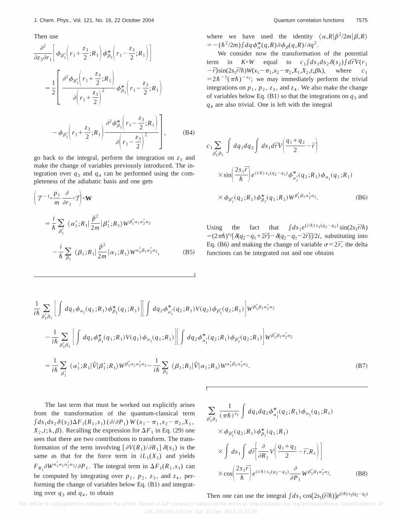
Then use

]2

]z3]r 1Ffb

18S r 11z3

2;R1Dfb1

* S r 12z3

2;R1D G

51

2F ]2fb18S r 11

z3

2;R1D

]S r 11z3

2 D 2 fb1* S r 12

z3

2;R1D

2fb18S r 11

z3

2;R1D ]2fb1

* S r 12z3

2;R1D

]S r 12z3

2 D 2 G , ~B4!

go back to the integral, perform the integration onz3 andmake the change of variables previously introduced. The in-tegration overq3 and q4 can be performed using the com-pleteness of the adiabatic basis and one gets

S T 21+p1

m

]

]r 1+TD +W

5i

\ (b18

^a18 ;R1up2

2mub18 ;R1&W

b18a1a28a2

2i

\ (b1

^b1 ;R1up2

2mua1 ;R1&W

a18b1a28a2, ~B5!

where we have used the identitya,Ru p2/2mub,R&52(\2/2m)*dqfa* (q,R)]fb(q,R)/]q2.

We consider now the transformation of the potentialterm in K+W equal to c1*ds1ds2d(s2)*drV(r 1

2 r )sin(2s1r/\)W(x12p1,x22p2,X1,X2,t;bl), where c1

52\21(p\)2n,; we may immediately perform the trivialintegrations onp1 , p2 , z3 , andz4 . We also make the changeof variables below Eq.~B1! so that the integrations onq3 andq4 are also trivial. One is left with the integral

c1 (b18b1

E dq1dq2E ds1drVS q11q2

22 r D

3sinS 2s1r

\ De~ i /\! s1(q22q1)fa18

* ~q2 ;R1!fa1~q1 ;R1!

3fb18~q2 ;R1!fb1

* ~q1 ;R1!Wb18b1a28a2. ~B6!

Using the fact that *ds1e( i /\) s1(q22q1) sin(2s1r/\)5(2p\)n,@d(q22q112r)2d(q22q122r)#/2i , substituting intoEq. ~B6! and making the change of variables52r , the deltafunctions can be integrated out and one obtains

1

i\ (b18b1

F E dq1fa1~q1 ;R1!fb1

* ~q1 ;R1!GF E dq2fa18

* ~q2 ;R1!V~q2!fb18~q2 ;R1!GWb18b1a28a2

21

i\ (b18b1

F E dq1fb1* ~q1 ;R1!V~q1!fa1

~q1 ;R1!GF E dq2fa18

* ~q2 ;R1!fb18~q2 ;R1!GWb18b1a28a2

51

i\ (b18

^a18 ;R1uVub18 ;R1&Wb18a1a28a22

1

i\ (b1

^b1 ;R1uVua1 ;R1&Wa18b1a28a2. ~B7!

The last term that must be worked out explicitly arisesfrom the transformation of the quantum-classical term*ds1ds2d (s2)DF1(R1 ,s1) (]/]P1) W (x12p1 ,x22p2 ,X1 ,X2 ,t;l,b). Recalling the expression forDF1 in Eq. ~29! onesees that there are two contributions to transform. The trans-formation of the term involving@]V(R1)/]R1# d(s1) is thesame as that for the force term iniL 1(X1) and yields

FR1]Wa18a1a28a2/]P1 . The integral term inDF1(R1 ,s1) can

be computed by integrating overp1 , p2 , z3 , and z4 , per-forming the change of variables below Eq.~B1! and integrat-ing overq3 andq4 , to obtain

(b18b1

1

~p\!n,E dq1dq2fa

18* ~q2 ;R1!fa1

~q1 ;R1!

3fb18~q2 ;R1!fb1

* ~q1 ;R1!

3E ds1E drF ]

]R1VS q11q2

22 r ,R1D G

3cosS 2s1r

\ De~ i /\! s1(q22q1)]

]P1Wb18b1a28a2. ~B8!

Then one can use the integral*ds1 cos@2s1(r/\)#e(i/\) s1(q22q1)

7575J. Chem. Phys., Vol. 121, No. 16, 22 October 2004 Quantum correlation functions

This article is copyrighted as indicated in the article. Reuse of AIP content is subject to the terms at: http://scitation.aip.org/termsconditions. Downloaded to IP:

136.165.238.131 On: Sat, 20 Dec 2014 22:22:30

5(2p\)n,@d(q22q112r)1d(q22q122r)#/2, make the changeof variables52r , and integrate out the delta functions tofind

1

2 F(b18

^a18 ;R1u]V~R1!

]R1ub18 ;R1&

]

]P1Wb18a1a28a2

1(b1

^b1 ;R1u]V~R1!

]R1ua1 ;R1&

]

]P1Wa18b1a28a2G . ~B9!

Analogous terms~but with opposite sign! are obtainedwhen considering the transformation of the terms dependingon x2 andX2 in Eq. ~27!.

Combining all terms and using the relationsFWab(R)

52^a;Ru¹RV(R)ub;R&5FWa 1(Ea2Eb)dab ,

2i

\ (b18

^a18 ;R1uS p2

2m1VD ub18 ;R1&W

b18a1a28a2

51i

\ (b1

^b1 ;R1uS p2

2m1VD ua1 ;R1&W

a18b1a28a2

52i

\@Ea

18~R1!2Ea1

~R1!#Wa18a1a28a2

52 iva18a1

~R1!Wa18a1a28a2, ~B10!

and introducing the definitionSa ib i5(Ea i

2Eb i)da ib i

@(P/M ) da ib i

#21, we find Eq.~32!.

1R. Kubo, J. Phys. Soc. Jpn.12, 570~1957!; R. Kubo, Rep. Prog. Phys.29,255 ~1966!.

2H. Mori, Prog. Theor. Phys.33, 423 ~1965!.3E. Rabani and D. Reichman, J. Chem. Phys.120, 1458~2004!.4S. A. Egorov, E. Rabani, and B. J. Berne, J. Phys. Chem. B103, 10978~1999!.

5A. A. Golosov, D. R. Reichman, and E. Rabani, J. Chem. Phys.118, 457~2003!.

6P. Pechukas, Phys. Rev.181, 166 ~1969!.7M. F. Herman, Annu. Rev. Phys. Chem.45, 83 ~1994!.8J. C. Tully, Modern Methods for Multidimensional Dynamics Computa-tions in Chemistry, edited by D. L. Thompson~World Scientific, NewYork, 1998!, p. 34.

9J. C. Tully, J. Chem. Phys.93, 1061~1990!; J. C. Tully, Int. J. QuantumChem. 25, 299 ~1991!; S. Hammes-Schiffer and J. C. Tully, J. Chem.Phys. 101, 4657 ~1994!; D. S. Sholl and J. C. Tully,ibid. 109, 7702~1998!.

10L. Xiao and D. F. Coker, J. Chem. Phys.100, 8646 ~1994!; D. F. Cokerand L. Xiao,ibid. 102, 496 ~1995!; H. S. Mei and D. F. Coker,ibid. 104,4755 ~1996!.

11F. Webster, P. J. Rossky, and P. A. Friesner, Comput. Phys. Commun.63,494 ~1991!; F. Webster, E. T. Wang, P. J. Rossky, and P. A. Friesner, J.Chem. Phys.100, 4835~1994!.

12T. J. Martinez, M. Ben-Nun, and R. D. Levine, J. Phys. Chem. A101,6389 ~1997!.

13A. Warshel and Z. T. Chu, J. Chem. Phys.93, 4003~1990!.14I. V. Aleksandrov, Z. Naturforsch. A36a, 902 ~1981!.15V. I. Gerasimenko, Repts. Ukranian Acad. Sci.10, 65 ~1981!; Teor. Mat.

Fiz. 150, 7 ~1982!.16W. Boucher and J. Traschen, Phys. Rev. D37, 3522~1988!.17W. Y. Zhang and R. Balescu, J. Plasma Phys.40, 199 ~1988!; R. Balescu

and W. Y. Zhang,ibid. 40, 215 ~1988!.18C. C. Martens and J.-Y. Fang, J. Chem. Phys.106, 4918 ~1996!; A.

Donoso and C. C. Martens, J. Phys. Chem.102, 4291~1998!; D. Kohenand C. C. Martens, J. Chem. Phys.111, 4343~1999!; 112, 7345~2000!.

19I. Horenko, C. Salzmann, B. Schmidt, and C. Schu¨tte, J. Chem. Phys.117,11075~2002!.

20C. Wan and J. Schofield, J. Chem. Phys.113, 7047~2000!.21R. Kapral and G. Ciccotti, J. Chem. Phys.110, 8919~1999!.22E. P. Wigner, Phys. Rev.40, 749 ~1932!; K. Imre, E. Ozizmir, M. Rosen-

baum, and P. F. Zwiefel, J. Math. Phys.5, 1097~1967!; M. Hillery, R. F.O’Connell, M. O. Scully, and E. P. Wigner, Phys. Rep.106, 121 ~1984!.

23K. Thompson and N. Makri, J. Chem. Phys.110, 1343~1999!.24D. Mac Kernan, G. Ciccotti, and R. Kapral, J. Chem. Phys.116, 2346

~2002!.25D. Mac Kernan, G. Ciccotti, and R. Kapral, J. Phys.: Condens. Matter14,

9069 ~2002!.26S. Nielsen, R. Kapral, and G. Ciccotti, J. Chem. Phys.112, 6543~2000!.27S. Nielsen, R. Kapral, and G. Ciccotti, J. Stat. Phys.101, 225 ~2000!.28A. Sergi, D. Mac Kernan, G. Ciccotti, and R. Kapral, Theor. Chem. Acc.

110, 49 ~2003!.29S. Nielsen, R. Kapral, and G. Ciccotti, J. Chem. Phys.115, 5805~2001!.30R. Kapral and G. Ciccotti, inBridging Time Scales: Molecular Simula-

tions for the Next Decade, 2001, A Statistical Mechanical Theory of Quan-tum Dynamics in Classical Environments, edited by P. Nielaba, M. Mare-schal, and G. Ciccotti~Springer, Berlin, 2003!, p. 445.

31A. Sergi and R. Kapral, J. Chem. Phys.118, 8566~2003!; ibid. 119, 12776~2003!.

32V. S. Filinov, Y. V. Medvedev, and V. L. Kamskyi, Mol. Phys.85, 711~1995!; V. S. Filinov, ibid. 88, 1517 ~1996!; ibid. 88, 1529 ~1996!; V. S.Filinov, S. Bonella, Y. E. Lozovik, A. Filinov, and I. Zacharov inClassicaland Quantum Dynamics in Condensed Phase Simulations, edited by B. J.Berne, G. Ciccotti, and D. F. Coker~World Scientific, Singapore, 1998!, p.667.

33S. A. Egorov, E. Rabani, and B. J. Berne, J. Chem. Phys.110, 5238~1999!.

7576 J. Chem. Phys., Vol. 121, No. 16, 22 October 2004 A. Sergi and R. Kapral

This article is copyrighted as indicated in the article. Reuse of AIP content is subject to the terms at: http://scitation.aip.org/termsconditions. Downloaded to IP:

136.165.238.131 On: Sat, 20 Dec 2014 22:22:30