Quantum-classical dualities in integrable systems

Andrei Zotov

Higher School of Economics and Steklov Mathematical Institute andSteklov Mathematical Institute of Russian Academy of Sciences, Moscow, Russia

Seminar at Department of Theoretical Physics

University of Szeged, Hungary

October 2019

Plan of the talk:

1. Algebraic Bethe ansatz for XXX spin chain

2. Classical Ruijsenaars-Schneider model

3. Duality

4. Quantum-quantum version of duality

5. Classical-classical version of duality

6. Further generalizations

Algebraic Bethe ansatz

1. Exchange relations (or RTT- or RLL- relations):

Rη00′(z, w)(T (z)⊗ I)(I ⊗ T (w)) = (I ⊗ T (w))(T (z)⊗ I)Rη00′(z, w) ,

R00′(z, w)T0(z)T0′(w) = T0′(w)T0(z)R00′(z, w) ,

T is a monodromy matrix operator-valued matrix in Mat(N,C), and R00′(z, w)is an invertible matrix from Mat(N,C)⊗2 with C-valued matrix elements depending

on spectral parameters z, w and the Planck constant η.

Example:

T (z) =

(A(z) B(z)C(z) D(z)

),

where A(z), B(z), C(c), D(z) are some operators.

R00′(z − w) =

1 + η

z−w 0 0 00 1 η

z−w 00 η

z−w 1 00 0 0 1 + η

z−w

(T (z)⊗ I) =

A(z) 0 B(z) 0

0 A(z) 0 B(z)C(z) 0 D(z) 0

0 C(z) 0 D(z)

(I ⊗ T (w)) =

A(w) B(w) 0 0C(w) D(w) 0 0

0 0 A(w) B(w)0 0 C(w) D(w)

Rη00′(z, w)(T (z) ⊗ I)(I ⊗ T (w)) = (I ⊗ T (w))(T (z) ⊗ I)Rη00′(z, w) , We get 16

commutation relations:

A(w)B(z) = (1 + ηz−w)B(z)A(w)− η

z−wB(w)A(z)

B(w)A(z) = (1 + ηz−w)A(z)B(w)− η

z−wA(w)B(z).....

1. Exchange relations (or RTT- or RLL- relations):

Rη00′(z, w)(T (z)⊗ I)(I ⊗ T (w)) = (I ⊗ T (w))(T (z)⊗ I)Rη00′(z, w) ,

R00′(z, w)T0(z)T0′(w) = T0′(w)T0(z)R00′(z, w) ,

T is a monodromy matrix operator-valued matrix in Mat(N,C), and R00′(z, w)

is an invertible matrix from Mat(N,C)⊗2 with C-valued matrix elements depending

on spectral parameters z, w and the Planck constant η.

2. The consistency condition for triple product T1(z1)T2(z2)T3(z3) (123→321in two ways) is the quantum Yang-Baxter equation:

Rη12(z12)Rη13(z13)Rη23(z23) = R

η23(z23)Rη13(z13)Rη12(z12) , zij = zi − zj

For example, the rational Yang's R-matrix

Rη00′(z − w) = I ⊗ I +

η

z − wP00′ , P00′ =

∑i,j

Eij ⊗ Eji .

Multiplying RTT-relations by R00′(z, w)−1

T0(z)T0′(w) = R00′(z, w)−1T0′(w)T0(z)R00′(z, w) ,

and taking the trace over the auxiliary spaces 0, 0′ we get

[T(z),T(w)] = 0

where

T(z) = tr T (z) .

is a transfer-matrix. Having an expansion of the form

T(z) =∑k

(z − z0)kIk

we obtain a set of commuting Hamiltonians

[Ik, Im] = 0 ∀k,m .

Spin chains:

t t t t t t t t t t t t t t t t t6 6 6 6 6 6 6 6

? ? ? ?? ? ? ? ?1nk

XXX Heisenberg chain

H =n∑

k=1

(σxkσ

xk+1 + σ

ykσ

yk+1 + σzkσ

zk+1

),

where the operators σαk = I⊗· · ·⊗σα⊗· · ·⊗I, α = x, y, z and σαn+1 = σα1 (closed

chain). The Hilbert space is H = V1 ⊗ ...⊗ Vn, For N = 2 Vk∼= C2, dimH = 2n.

R00′(z − w) =

1 + η

z−w 0 0 00 1 η

z−w 00 η

z−w 1 00 0 0 1 + η

z−w

To each site we assign the Lax operator Lk(z):

Lk(z) =

(I + η

zσzk

ηzσ−k

ηzσ

+k I − η

zσzk

)= R0k(z) ∈Mat(2,C)⊗ End(H) ∼= Mat(2,C)⊗(n+1)

T (z) =

(A(z) B(z)C(z) D(z)

),

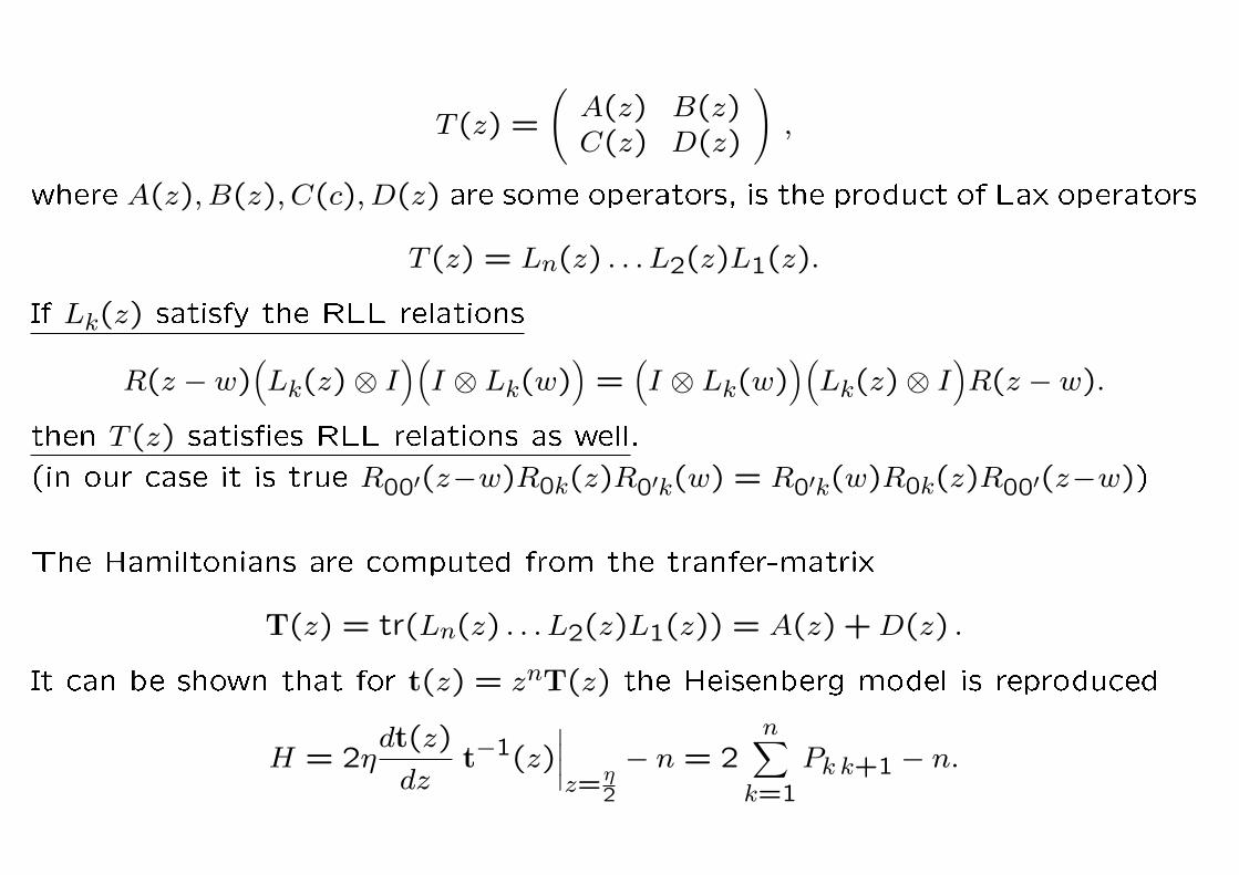
where A(z), B(z), C(c), D(z) are some operators, is the product of Lax operators

T (z) = Ln(z) . . . L2(z)L1(z).

If Lk(z) satisfy the RLL relations

R(z − w)(Lk(z)⊗ I

)(I ⊗ Lk(w)

)=(I ⊗ Lk(w)

)(Lk(z)⊗ I

)R(z − w).

then T (z) satises RLL relations as well.

(in our case it is true R00′(z−w)R0k(z)R0′k(w) = R0′k(w)R0k(z)R00′(z−w))

The Hamiltonians are computed from the tranfer-matrix

T(z) = tr(Ln(z) . . . L2(z)L1(z)) = A(z) +D(z) .

It can be shown that for t(z) = znT(z) the Heisenberg model is reproduced

H = 2ηdt(z)

dzt−1(z)

∣∣∣∣z=η

2

− n = 2n∑

k=1

Pk k+1 − n.

Generalized spin chain

Inhomogeneous twisted XXX chain:

T (z) = gLn(z − qn) . . . L1(z − q1) ,

where q1, ..., qn are inhomogeneity parameters and g =N∑a=1

Eaaga (diagonal)

constant twist matrix. It comes from the symmetry of R-matrix:

R(z − w)(g ⊗ g

)=(g ⊗ g

)R(z − w).

The generating function of commuting integrals of motion (the transfer matrix)

depending on the spectral parameter z being of the form

T(z) = tr0

(g(0)R0n(z − qn) . . . R02(z − q2)R01(z − q1)

)= tr g · I +

n∑j=1

ηHj

z − qj,

Rij(z) = I +η

zPij , Pij =

N∑a,b=1

E(i)ab E

(j)ba .

Its residues are non-local Hamiltonians:

Hi = Ri i−1(qi−qi−1) . . . Ri1(qi−q1)g(i)Rin(qi−qn) . . . Ri i+1(qi−qi+1)

Idea of the Bethe ansatz

Write down commutation relations:

[T jk(u), T jk(v)] = 0, j, k = 1,2,

A(w)B(z) = (1 + ηz−w)B(z)A(w)− η

z−wB(w)A(z)

B(w)A(z) = (1 + ηz−w)A(z)B(w)− η

z−wA(w)B(z).....

Recall that the elements of the monodromy matrices act in some Hilbert space

H. In the framework of the algebraic Bethe ansatz, very small requirements are

imposed on this space. Namely, it is necessary that there exist a vacuum vector

such that (a(z), d(z) below are some C-valued functions)

A(z)|0〉 = a(z)|0〉, D(z)|0〉 = d(z)|0〉, C(z)|0〉 = 0.

The vacuum vector for XXX spin chain: all spins up in N = 2 case, i.e.

|0〉 =(

10

)1⊗ · · · ⊗

(10

)n.

We look for the eigenvectors of the transfer-matrix ψ in the form

ψ = B(µ1)...B(µn1)|0〉 , (A(z) +D(z))ψ = λ(z, µ)ψ .

The vacuum vector is the eigenvector for the operators A(z) and D(z), while

the operator C(z) annihilates it. The action of the operator B(z) onto the

vacuum is free. It is assumed that acting with this operator on vacuum we

generate all the space H. The set of parameters µ1, ..., µn1 to be determined

Bethe roots.

Compute the action of the operator A(z) onto the vector ψ:

A(z)B(µ1)...B(µn1)|0〉 =

= a(z)Λ(z|µ)B(µ1)...B(µn1)|0〉+∑n1k=1 a(µk)Λk(z|µ)B(z)

∏l 6=k

B(µl)|0〉.

After computing the same for D(z) and summing up we get

T(z)B(µ1)...B(µn1)|0〉 =(a(z)Λ(v|µ) + d(v)Λ(z|µ)

)B(µ1)...B(µn1)|0〉

+∑nk=1

(a(µk)Λk(z|µ) + d(uk)Λk(z|µ)

)B(z)

∏l 6=k

B(µl)|0〉.

Conditions for vanishing of the unwanted terms Bethe equations:

a(µk)Λk(z|µ) + d(µk)Λk(z|µ) = 0, k = 1, . . . , n1

The generating function of the eigenvalues of transfer-matrix:

λ(z|µ) = a(z)Λ(z|µ) + d(z)Λ(z|µ) .

Example the Bethe equations (BE):

g1

g2

n∏k=1

µα − qk + η

µα − qk=

n1∏γ 6=α

µα − µγ + η

µα − µγ − η, α = 1 , ... , n1 .

The eigenvalues:

1

ηHXXX

i = g1

n∏k 6=i

qi − qk + η

qi − qk

n1∏γ=1

qi − µγ − ηqi − µγ

, i = 1 , . . . , n,

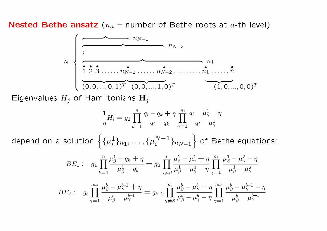
Nested Bethe ansatz (na number of Bethe roots at a-th level)

N

︷ ︸︸ ︷ nN−1︷ ︸︸ ︷ nN−2...︷ ︸︸ ︷ n1•1•2•3 . . . . . .

•nN−1 . . . . . .

•nN−2 . . . . . . . . .

•n1 . . . . . .

•n︸ ︷︷ ︸ ︸ ︷︷ ︸ ︸ ︷︷ ︸

(0,0, ...,0,1)T (0,0, ...,1,0)T (1,0, ...,0,0)T

Eigenvalues Hj of Hamiltonians Hj

1

ηHi = g1

n∏k=1

qi − qk + η

qi − qk

n1∏γ=1

qi − µ1γ − η

qi − µ1γ

depend on a solution

µ1

i n1, . . . , µN−1i nN−1

of Bethe equations:

BE1 : g1

n∏k=1

µ1β − qk + η

µ1β − qk

= g2

n1∏γ 6=β

µ1β − µ1

γ + η

µ1β − µ1

γ − η

n2∏γ=1

µ1β − µ2

γ − ηµ1β − µ2

γ

BE b : gb

nb−1∏γ=1

µbβ − µb−1γ + η

µbβ − µb−1γ

= gb+1

nb∏γ 6=β

µbβ − µbγ + η

µbβ − µbγ − η

nb+1∏γ=1

µbβ − µb+1γ − η

µbβ − µb+1γ

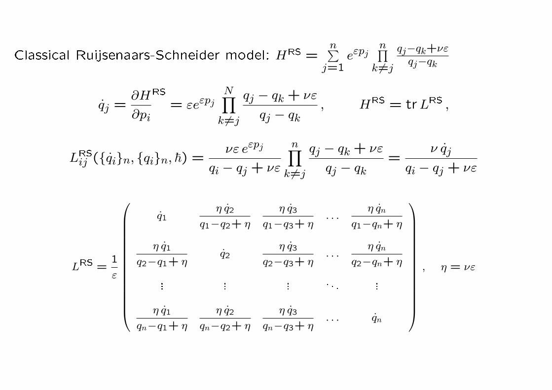
Classical Ruijsenaars-Schneider model: HRS =n∑

j=1eεpj

n∏k 6=j

qj−qk+νεqj−qk

qj =∂H

∂pi

RS

= εeεpjN∏k 6=j

qj − qk + νε

qj − qk, HRS = trLRS ,

LRSij (qin, qin, ~) =νε eεpj

qi − qj + νε

n∏k 6=j

qj − qk + νε

qj − qk=

ν qj

qi − qj + νε

LRS =1

ε

q1η q2

q1−q2+ η

η q3

q1−q3+ η. . .

η qn

q1−qn+ η

η q1

q2−q1+ ηq2

η q3

q2−q3+ η. . .

η qn

q2−qn+ η

... ... ... . . . ...

η q1

qn−q1+ η

η q2

qn−q2+ η

η q3

qn−q3+ η. . . qn

, η = νε

Factorization of the Ruijsenaars-Schneider Lax matrix:

Introduce the diagonal matrices D0 and D~

(D0)ij(uK) = δijK∏k 6=i

(ui − uk) ,

(D~)ij(uK) = δijK∏k 6=i

(ui − uk + ~) ,

i , j = 1 , ... ,K ,

the Vandermonde matrix Vij(uK) = ui−1j , i , j = 1 , ... ,K, and the triangular

matrix

(C~,K)ij =

(i− 1)! ~i−j

(j − 1)!(i− j)!, j ≤ i ,

0 , j > i ,

V (u+ eK~) = C~,KV (u)eK = (1, ...,1)

Then the following matrix has all eigenvalues equal to g:

(due to det(L− λ) = det(C~ − λ))

Lij(xN , g) =g ~

xi − xj + ~

N∏k 6=j

xj − xk + ~xj − xk

, i , j = 1 , ... , N

L(xN , g) = g D−1~ (xN)V T (xN + ~ eN)

(V T

)−1(xN)D~(xN) =

= g D−1~ (xN)V T (xN)CT~,N

(V T

)−1(xN)D~(xN) , eN = (1, ...,1)

and similarly for

Lαβ(yM , g) =g ~

yα − yβ + ~

M∏γ 6=β

yβ − yγ − ~yβ − yγ

, α , β = 1 , ... ,M .

L(yM , g) = g D0(yM)V −1(yM)V (yM − ~ eM)D−10 (yM) =

= g D0(yM)V −1(yM)C−~,M V (yM)D−10 (yM) .

Quantum-classical duality

On the quantum side: consider the inhomogeneous GL(N) generalized spin

chain of XXX type on n sites with inhomogeneity parameters qi and vector

representations at each site. Let us impose twisted boundary conditions with the

twist matrix g = diag(g1, . . . , gN), with the generating function of commuting

integrals of motion (the transfer matrix) depending on the spectral parameter

z being of the form

T(z) = tr0

(g(0)R0n(z − qn) . . . R02(z − q2)R01(z − q1)

)= tr g · I +

n∑j=1

ηHj

z − qj,

Rij(z) = I +η

zPij , Pij =

N∑a,b=1

E(i)ab E

(j)ba .

Its residues are (non-local) Hamiltonians

Hi = Ri i−1(qi−qi−1) . . . Ri1(qi−q1)g(i)Rin(qi−qn) . . . Ri i+1(qi−qi+1)

N

︷ ︸︸ ︷ nN−1︷ ︸︸ ︷ nN−2...︷ ︸︸ ︷ n1•1•2•3 . . . . . .

•nN−1 . . . . . .

•nN−2 . . . . . . . . .

•n1 . . . . . .

•n︸ ︷︷ ︸ ︸ ︷︷ ︸ ︸ ︷︷ ︸

(0,0, ...,0,1)T (0,0, ...,1,0)T (1,0, ...,0,0)T

Eigenvalues Hj of Hamiltonians Hj

1

ηHi = g1

n∏k=1

qi − qk + η

qi − qk

n1∏γ=1

qi − µ1γ − η

qi − µ1γ

depend on a solution

µ1

i n1, . . . , µN−1i nN−1

of Bethe equations:

BE1 : g1

n∏k=1

µ1β − qk + η

µ1β − qk

= g2

n1∏γ 6=β

µ1β − µ1

γ + η

µ1β − µ1

γ − η

n2∏γ=1

µ1β − µ2

γ − ηµ1β − µ2

γ

, β = 1...n1

BE b : gb

nb−1∏γ=1

µbβ − µb−1γ + η

µbβ − µb−1γ

= gb+1

nb∏γ 6=β

µbβ − µbγ + η

µbβ − µbγ − η

nb+1∏γ=1

µbβ − µb+1γ − η

µbβ − µb+1γ

, β = 1...nb

The claim is that under the substitution:

1. η is the Planck constant

2. positions of RS particles qi are inhomogeneous parameters

3. the velocities are eigenvalues of quantum Hamitonians

qj =1

ηHj

(qin; µ1

i n1, . . . , µN−1i nN−1

), j = 1 , ... , n , (1)

where the set of µai 's is any solution of the nested BE for the spin chain, the

eigenvalues of the Lax matrix are(g1 , . . . , g1︸ ︷︷ ︸

n−n1

, g2 , . . . , g2︸ ︷︷ ︸n1−n2

, . . . , gN−1 , . . . , gN−1︸ ︷︷ ︸nN−2−nN−1

, gN , . . . , gN︸ ︷︷ ︸nN−1

).

(2)

i.e.

det

[LRS

(1

η

Hjn,qjn, ηε

)∣∣∣∣BE− λ

]=

N∏a=1

(ga − λ)Ma, (3)

where M1 = n−n1, Ma = na−1−na (2 ≤ a ≤ N)

On the classical side: consider the RS model with coupling constant η and the

number of particles, n, equal to the number of sites of the GL(N) spin chain.

The Lax matrix of the model is n× n:

LRSij (qin, qin, η) =η qj

qi − qj + η. (4)

Statement: under substitution

qj =1

ηHj

(qin; µ1

i n1, . . . , µN−1i nN−1

), j = 1 , ... , n ,

where the sets µai are some solutions of BE, the eigenvalues of Lax matrix

acquire the form:(g1 , . . . , g1︸ ︷︷ ︸

n−n1

, g2 , . . . , g2︸ ︷︷ ︸n1−n2

, . . . , gN−1 , . . . , gN−1︸ ︷︷ ︸nN−2−nN−1

, gN , . . . , gN︸ ︷︷ ︸nN−1

).

GL(2) :(g1 , . . . , g1︸ ︷︷ ︸spin down

, g2 , . . . , g2︸ ︷︷ ︸spin up

).

Idea of the proof. Let us introduce the following pair of matrices:

Lij(xiN , yiM , g) =g ~

xi − xj + ~

N∏k 6=j

xj − xk + ~xj − xk

M∏γ=1

xj − yγxj − yγ + ~

, i , j = 1 , ... , N

and

Lαβ(yiM , xiN , g) =g ~

yα − yβ + ~

M∏γ 6=β

yβ − yγ − ~yβ − yγ

N∏k=1

yβ − xkyβ − xk − ~

, α, β = 1 , ... ,M

QC-duality is based on algebraic relation between determinants of L and L:

detN×N

(L (xiN , yiM , g)− λ

)= (g − λ)N−M det

M×M

(L (yiM , xiN , g)− λ

)For M = 0 (factorization of the Ruijsenaars Lax matrix)

detN×N

(L (xiN , yi0, g)− λ

)= (g − λ)N

LRS =1

η

H1η H2

q1−q2+ η

η H3

q1−q3+ η. . .

η Hn

q1−qn+ η

η H1

q2−q1+ ηH2

η H3

q2−q3+ η. . .

η Hn

q2−qn+ η

... ... ... . . . ...

η H1

qn−q1+ η

η H2

qn−q2+ η

η H3

qn−q3+ η. . . Hn

qj =1

ηHj = g1

n∏k=1

qj − qk + η

qj − qk

n1∏γ=1

qj − µ1γ − η

qj − µ1γ

where µai solutions of BE. We want to prove that eigenvalues of LRS are(g1 , . . . , g1︸ ︷︷ ︸

M1

, g2 , . . . , g2︸ ︷︷ ︸M2

, . . . , gN−1 , . . . , gN−1︸ ︷︷ ︸MN−1

, gN , . . . , gN︸ ︷︷ ︸MN

).

L(0)ij = LRSij (

1

ηHXXX

j n, qin, η) =η g1

qi − qj + η

n∏k 6=j

qj − qk + η

qj − qk

n1∏γ=1

qj − µ1γ − η

qj − µ1γ

= Lij(qi−ηn, µ1αn1, g1) ,

L(1)αβ = Lαβ(µ1

αn1, qi−ηn, g1) =η g1

µ1α − µ1

β + η

n1∏γ 6=β

µ1β − µ

1γ − η

µ1β − µ1

γ

n∏k=1

µ1β − qk + η

µ1β − qk

,

where α, β = 1 , ... , n1.

detn×n

(L(0) − λ) = (g1 − λ)n−n1 detn1×n1

(L(1) − λ) .

Next, impose the Bethe equations

L(1)αβ

∣∣∣∣BE1

=η g2

µ1α − µ1

β + η

n1∏γ 6=β

µ1β − µ

1γ + η

µ1β − µ1

γ

n2∏γ=1

µ1β − µ

2γ − η

µ1β − µ2

γ, α, β = 1 , ... , n1 ,

i.e.,

L(1)∣∣∣BE1

= L(µ1α−ηn1, µ

2αn2, g2) .

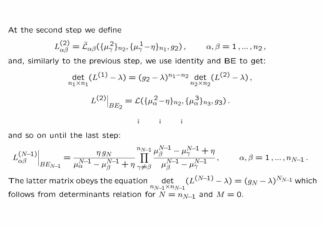
At the second step we dene

L(2)αβ = Lαβ(µ2

γ n2, µ1γ −ηn1, g2) , α, β = 1 , ... , n2 ,

and, similarly to the previous step, we use identity and BE to get:

detn1×n1

(L(1) − λ) = (g2 − λ)n1−n2 detn2×n2

(L(2) − λ) ,

L(2)∣∣∣BE2

= L(µ2α−ηn2, µ

3αn3, g3) .

... ... ...

and so on until the last step:

L(N−1)αβ

∣∣∣∣BEN−1

=η gN

µN−1α − µN−1

β + η

nN−1∏γ 6=β

µN−1β − µN−1

γ + η

µN−1β − µN−1

γ, α, β = 1 , ... , nN−1 .

The latter matrix obeys the equation detnN−1×nN−1

(L(N−1) − λ) = (gN − λ)NN−1 which

follows from determinants relation for N = nN−1 and M = 0.

Similar relation between the classical Calogero-Moser and quantum Gaudin

models appears in the limit ε→ 0 (η = νε). Then

LCMij = limε→0

LRSij − δijε

= δij qi + ν1− δijqi − qj

, qi = pi + ν∑k 6=i

1

qi − qk

HG

i =N∑a=1

vaE(i)aa +

n∑j 6=i

ν Pijqi − qj

= limε→0

Hi(qin, g = eεv, εη)− εηC(i)1

ηε2

where C(i)1 =

N∑a=1

e(i)aa è Pij =

∑Na,b=1E

(i)ab E

(j)ba

SpecLCM(

1~HG

j

n,qjn, ν = ~

)∣∣∣∣BE

=

=(v1 , . . . , v1︸ ︷︷ ︸

n−n1

, v2 , . . . , v2︸ ︷︷ ︸n1−n2

, . . . , vN−1 , . . . , vN−1︸ ︷︷ ︸nN−2−nN−1

, vN , . . . , vN︸ ︷︷ ︸nN−1

)

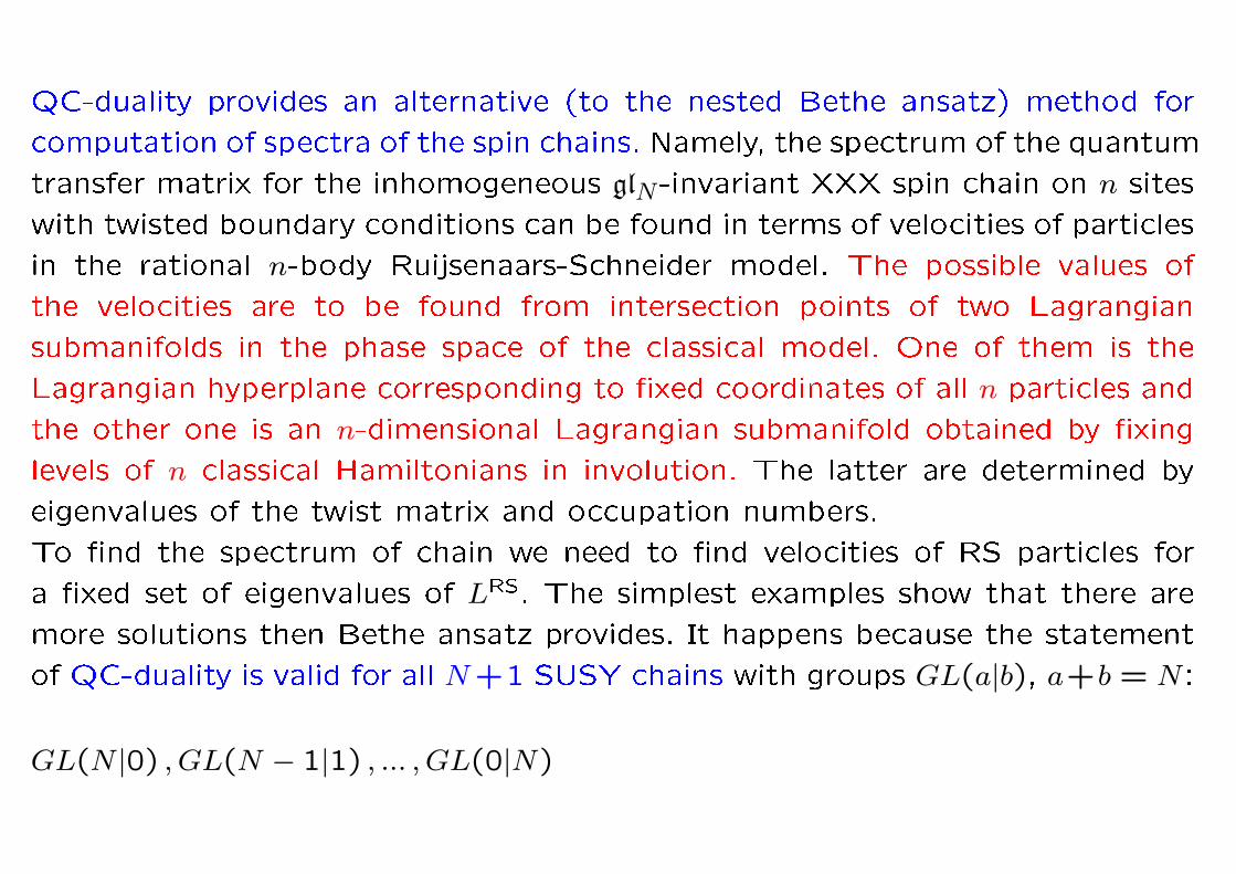
QC-duality provides an alternative (to the nested Bethe ansatz) method for

computation of spectra of the spin chains. Namely, the spectrum of the quantum

transfer matrix for the inhomogeneous glN-invariant XXX spin chain on n sites

with twisted boundary conditions can be found in terms of velocities of particles

in the rational n-body Ruijsenaars-Schneider model. The possible values of

the velocities are to be found from intersection points of two Lagrangian

submanifolds in the phase space of the classical model. One of them is the

Lagrangian hyperplane corresponding to xed coordinates of all n particles and

the other one is an n-dimensional Lagrangian submanifold obtained by xing

levels of n classical Hamiltonians in involution. The latter are determined by

eigenvalues of the twist matrix and occupation numbers.

To nd the spectrum of chain we need to nd velocities of RS particles for

a xed set of eigenvalues of LRS. The simplest examples show that there are

more solutions then Bethe ansatz provides. It happens because the statement

of QC-duality is valid for all N+1 SUSY chains with groups GL(a|b), a+b = N :

GL(N |0) , GL(N − 1|1) , ... , GL(0|N)

The Bethe ansatz in SUSY case is slightly more complicated, but the statement

is the same for any chain from the set.

Inverse problem: nd velocities from xed set of eigenvalues of the Lax matrix

(i.e. action variables) and coordintes qk.

det1≤i,j≤n

(λδij −

ηHiqi − qj + η

)=

N∏a=1

(λ− ga)Ma , Ma = na−1 − na

∑1≤i1<...<id≤n

Hi1 . . . Hid

∏1≤α<β≤d

1−η2

(qiα − qiβ)2

−1

= ed(Pj) ,

where Pj =∑aMagka, and ed elementary symmetric functions. These algebraic

equations describe spectrum of all N + 1 SUSY quantum chains.

Thus, we come to correspondence between classical many-body systems

and the set of spin chains. The desired simplication of the nested Bethe

ansatz is in fact replaced by another problem untangling of solutions between

dierent chains.

We have described the quantum-classical duality

What is quantum-quantum version?

And what is classical-classical version?

The quantum-quantum case is the Matsuo-Cherednik type correspondence

between the quantum Knizhnik-Zamolodchikov equations associated with GL(N)

and n-particle quantum Ruijsenaars-Schneider model, with n being not necessarily

equal to N .

qKZ-Ruijsenaars correspondence:

The quantum Knizhnik-Zamolodchikov (qKZ) equations:

eη~∂xi∣∣∣∣Φ⟩ = K(~)

i

∣∣∣∣Φ⟩, i = 1, . . . , n

K(~)i = Ri i−1(xi−xi−1+η~) . . .Ri1(xi−x1+η~)g(i)Rin(xi−xn) . . .Ri i+1(xi−xi+1)

Rij(x) =xI + ηPijx+ η

, Rij(x)Rji(−x) = id

Solutions can be found in the form∣∣∣∣Φ⟩ =∑σ∈Sn

Φσ

∣∣∣∣eσ⟩, ∣∣∣∣eσ⟩ = eσ(1) ⊗ eσ(2) ⊗ . . .⊗ eσ(n),

where ea are standard basis vectors in V = CN =⊕Na=1 Cea and Sn is the

symmetric group.

There is a natural weight decomposition of the Hilbert space of the spin chain:

V = V ⊗n =⊕

M1,...,MN

V(Ma)

dened by operators

Ma =n∑l=1

e(l)aa , [Ma,Mb] = [Hi,Ma] = 0

The basis vectors in V(Ma) are

∣∣∣∣J⟩ = ej1 ⊗ ej2 ⊗ . . .⊗ ejn, where the number

of indices jk such that jk = a is equal to Ma for all a = 1, . . . , N .

Important property:

n∑i=1

Hi =n∑i=1

g(i) =N∑a=1

gaMa

Statement: Let

∣∣∣∣Φ⟩ =∑J

ΦJ

∣∣∣∣J⟩ be a solution of qKZ in weight subspace

V(Ma). Then for E =N∑a=1

Maga and

Ψ =∑J

ΦJ =⟨

Ω∣∣∣∣Φ⟩ , ⟨

Ω∣∣∣∣ =

∑J

⟨J

∣∣∣∣we have

n∑i=1

n∏j 6=i

xi−xj+η

xi − xjΨ(x1, . . . , xi+η~, . . . , xn) = EΨ(x1, . . . , xn).

The proof is based on the property of Ma, relation R(x) = x+ηx R(x) = I + η

xP

and

⟨Ω∣∣∣∣Pij =

⟨Ω∣∣∣∣. From the latter we have

⟨Ω∣∣∣∣Rij(x) =

⟨Ω∣∣∣∣xI + ηPijx+ η

=⟨

Ω∣∣∣∣

and therefore,

⟨Ω∣∣∣∣K(~)

i =⟨

Ω∣∣∣∣K(0)

i . Recall that in spin chain we used R(x).

eη~∂xi⟨

Ω∣∣∣∣Φ⟩ = eη~∂xiΨ =

⟨Ω∣∣∣∣K(~)

i

∣∣∣∣Φ⟩ =⟨

Ω∣∣∣∣K(0)

i

∣∣∣∣Φ⟩.Therefore, multiplying by

n∏j 6=i

xi − xj + η

xi − xjand summing over i, we get:

n∑i=1

n∏j 6=i

xi − xj + η

xi − xj

eη~∂xiΨ =n∑i=1

n∏j 6=i

xi − xj + η

xi − xj

⟨Ω∣∣∣∣K(0)

i

∣∣∣∣Φ⟩

=n∑i=1

⟨Ω∣∣∣∣Hi

∣∣∣∣Φ⟩ =n∑i=1

⟨Ω∣∣∣∣g(i)

∣∣∣∣Φ⟩ =N∑a=1

ga

⟨Ω∣∣∣∣Ma

∣∣∣∣Φ⟩ =

N∑a=1

gaMa

Ψ.

A natural conjecture is that Ψ is the common eigenfunction for all higher

Ruijsenaars Hamiltonians Hk with the eigenvalues Ek =∑aMagka. It appears to

be true.

Classical-classical version

What is the classical analogue of the KZ equations? The answer: it is the

classical Schlesinger system non-autonomous version of the Gaudin model.

The Gaudin model:

L(z) = Λ +n∑i=1

Si

z − qi, Λ = diag(λ1, ..., λN) ,

The Hamiltonians follow from tr(L2(z)):

Hi = tr(SiΛ) +n∑

j:j 6=i

tr(SiSj)

qi − qj, i = 1, ..., n .

Equations of motion

∂tiSj =

[Si, Sj]

qi − qi, i 6= j , ∂tiS

i = −[Si,Λ]−n∑k 6=i

[Si, Sk]

qi − qk, i 6= j

are written in the Lax form

∂tiL(z) = [L(z),Mi(z)] , Mi(z) = −Si

z − qi.

The Schlesinger system is obtained by replacing time variables with the positions

of marked points qi:

∂qiSj =

[Si, Sj]

qi − qi, i 6= j , ∂qiS

i = −[Si,Λ]−n∑k 6=i

[Si, Sk]

qi − qk, i 6= j

The equations of motion are equivalent to the monodromy preserving equations

∂qiL(z)− ∂zMi(z) = [L(z),Mi(z)]

with the same Lax pairs as in Gaudin case.

The quantization of the Gaudin Hamiltonians is given as follows:

(tr(SiSj) =∑a,b S

iabS

jba →

∑ab e

iabe

jba = Pij)

Hi =l∑

c=1

λce(i)cc +

k∑j:j 6=i

Pij

qi − qj, i = 1, ..., k .

For the quantum Schlesinger system we have non-stationary Schrodinger equations(κ∂qi −Hi

)|Ψ〉 = 0 , i = 1, ..., k .

which are just the KZ equations.

Calogero-Moser model in the form of Gaudin-Schlesinger system:

Consider the Lax matrix of the classical Calogero-Moser model

Lij = δijpj + (1− δij)ν

qi − qj,

and its eigenvalue problem

LΨ = ΨΛ , Λ = diag(λ1, ..., λn) ,

where Ψ is a matrix of eigenvectors. Introduce "ctitious"spectral parameter

z through the gauge transformation:

Lij → L′ij = Lijz−qiz−qj = Lij + Lij(qi − qj) 1

z−qj

L′(z) = (z −Q)L(z −Q)−1 = L+ [L,Q](z −Q)−1 = L−O(z −Q)−1,

where Q = diag(q1, ..., qn) and O = [Q,L]: Oij = ν(1− δij).

L′(z) = L−n∑

a=1

Oa

z − qa, Oaij = ν(1− δij)δaj .

L′′(z) = Ψ−1L′(z)Ψ = Λ−n∑

a=1

Ψ−1OaΨ

z − qa

In the Schlesinger case the Lax matrix is replaced by the connection L→ ∂z+L.

The same gauge transformations results in

∂z + L′′(z) = ∂z + Ψ−1L′(z)Ψ = ∂z + Λ− νn∑

a=1

Ψ−1OaΨ

z − qa,

where Oaij = ν(1− δij)δaj + δijδaj. The Hamiltonians

Ha = tr(LOa)−∑c6=a

tr(OaOc)qa − qc

Since tr(LOa) = pa and tr(OaOc) = δac + ν(1− δac), we get

Ha = pa −∑c6=a

ν

qa − qc= qa

Symplectic form: ∑i

dHi ∧ dti =∑i

dpi ∧ dqi.

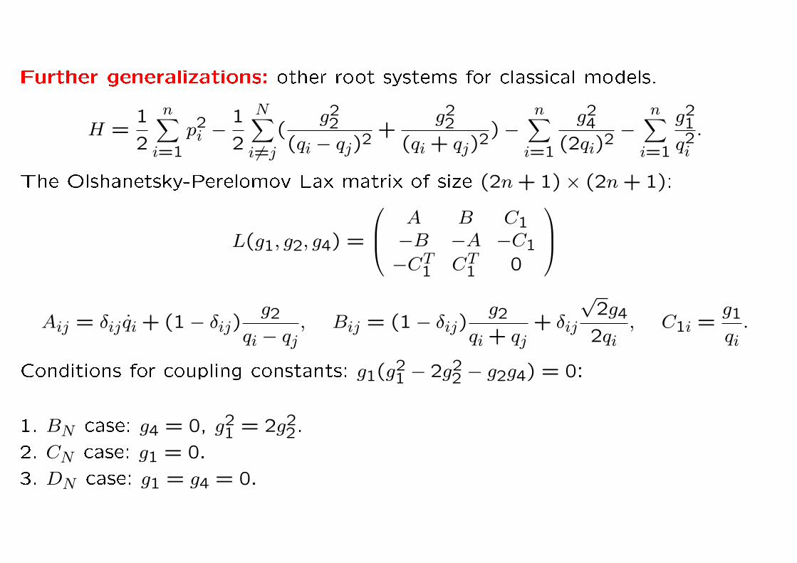
Further generalizations: other root systems for classical models.

H =1

2

n∑i=1

p2i −

1

2

N∑i 6=j

(g2

2

(qi − qj)2+

g22

(qi + qj)2)−

n∑i=1

g24

(2qi)2−

n∑i=1

g21

q2i

.

The Olshanetsky-Perelomov Lax matrix of size (2n+ 1)× (2n+ 1):

L(g1, g2, g4) =

A B C1−B −A −C1−CT1 CT1 0

Aij = δij qi + (1− δij)g2

qi − qj, Bij = (1− δij)

g2

qi + qj+ δij

√2g4

2qi, C1i =

g1

qi.

Conditions for coupling constants: g1(g21 − 2g2

2 − g2g4) = 0:

1. BN case: g4 = 0, g21 = 2g2

2.

2. CN case: g1 = 0.

3. DN case: g1 = g4 = 0.

In this cases on the quantum side we deal with open spin chains (with boundaries).

The boundaries are described by reection equations:

R12(u1 − u2)K−1 (u1)R12(u1 + u2)K−2 (u2) =

= K−2 (u2)R12(u1 + u2)K−1 (u1)R12(u1 − u2),

and the transfer-matrix is

T(u) = tr0

(K+0 (u)R01(u− q1)..R0N(u− qN)K−0 (u)R0N(u+ qN)..R01(u+ q1)).

Consider K-matrices

K−(u) =

(1 + α

u 00 −1 + α

u

), K+(u) =

1 + β−u−~ 0

0 −1 + β−u−~

,The Gaudin limit of the eigenvalues and Bethe equations are of the form:

tG(z) =n∑i=1

(HGi

z − qi−

HGi

z + qi

)

HGi = (α− β)

1

qi+

n∑k 6=i

(1

qi − qk+

1

qi + qk)−

n1∑k=1

(1

qi − µk+

1

qi + µk),

And the Bethe equations are

(α− β)2

µi+

n∑k=1

(1

µi − qk+

1

µi + qk) =

2

µi+

n1∑k 6=i

(2

µi − µk+

2

µi + µk),

The statement of the QC-duality is as follows: Consider the CN Calogero-

Moser Lax matrix (of size 2n × 2n). Plugging HGi = qi and g2 = ~, g4 =√

2~(α−β), g1 = 0 we obtain that such matrix has all zero eigenvalues on-shell

Bethe equations:

det(L(0, ~,√

2~(α− β))− λ) = λ2n .

Similar statements are valid for BN and DN models.

The talk is based on

A. Gorsky, A. Zabrodin, A. Zotov, Spectrum of quantum transfer matrices via classical many-

body systems, JHEP 01 (2014) 070; arXiv: 1310.6958;

Zengo Tsuboi, Anton Zabrodin, Andrei Zotov, Supersymmetric quantum spin chains and

classical integrable systems, JHEP 05 (2015) 086; arXiv: 1412.2586;

M. Beketov, A. Liashyk, A. Zabrodin, A. Zotov, Trigonometric version of quantumclassical

duality in integrable systems, Nuclear Physics B, 903 (2016) 150163, arXiv: 1510.07509;

A. Liashyk, D. Rudneva, A. Zabrodin, A. Zotov, Asymmetric 6-vertex model and classical

Ruijsenaars-Schneider system of particles, Theoret. and Math. Phys., 192:2 (2017) 1141-1153;arXiv:1611.02497;

A. Zabrodin, A. Zotov, KZ-Calogero correspondence revisited, J. Phys. A: Math. Theor. 50(2017) 205202, arXiv:1701.06074;

A. Zabrodin, A. Zotov, QKZ-Ruijsenaars correspondence revisited, Nuclear Physics B, 922(2017) 113-125; arXiv:1704.04527.

M. Vasilyev, A. Zotov, On factorized Lax pairs for classical many-body integrable systems,Reviews in Mathematical Physics, 31:6 (2019) 1930002, 45 pp; arXiv:1804.02777.

M. Vasilyev, A. Zotov, Quantum-classical duality for boundary Gaudin models, to appear

Thank you!