Quantitative ornithologywith a commercial marine radar:

standard-target calibration, target detection and tracking,

andmeasurement of echoes from individuals and flocks

Samuel S. Urmy* and JosephD.Warren

Stony BrookUniversity, School ofMarine andAtmospheric Sciences, 239MontaukHwy., Southampton, NY 11901, USA

Summary

1. Marine surveillance radars are commonly used for radar ornithology, but they are rarely calibrated. This pre-

vents them frommeasuring the radar cross-sections (RCS) of the birds under study. Furthermore, if the birds are

aggregated too closely for the radar to resolve them individually, the bulk volume reflectivity cannot be trans-

lated into a numerical density.

2. We calibrated a commercial off-the-shelf marine radar, using a standard spherical target of knownRCS.Once

calibrated, the radar was used to measure the RCS of common and roseate terns (Sterna hirundo L. and Sterna

dougallii Montagu) tracked from a land-based installation at their breeding colony on Great Gull Island, NY,

USA. We also integrated echoes from flocks of terns, comparing these total flock cross-sections with visual

counts from photos taken at the same time as the radarmeasurements.

3. The radar’s calibration parameters were determined with 1% error. RCS measurements made after calibra-

tion were expected to be accurate within�2 dB.Mean tern RCSwas estimated at�28 dB relative to one square

meter (dBsm), agreeing inmagnitudewith a simple theoreticalmodel. RCSwas 3–4 dB higher when birds’ aspect

angles were broadside to the radar beam compared with head- or tail-on. Integrated flock cross-section was lin-

early related to the number of birds. The slope of this line, an independent estimate of RCS, was �32 dBsm,

within an order ofmagnitude of the estimate from individual birds, and near themiddle of the frequency distribu-

tion ofRCS values.

4. These results indicate that a calibrated marine radar can count the birds in an aggregation via echo integra-

tion. Field calibration of marine radars is practical, enables useful measurements, and should be done more

often.

Key-words: echo integration, Great Gull Island, radar cross-section, radar equation, radar

ornithology, random forest, seabirds, terns, track while scan

Introduction

Radar has been used to study the movements and distribution

of birds since the end of the Second World War (Eastwood

1967), and is a key technique in the growing field of aeroecol-

ogy (Chilson et al. 2012). At the largest scale, networks of

weather radars have revealed continental patterns of bird

migration (Bruderer 1997; Chilson et al. 2012; Shamoun-

Baranes et al. 2014). Radar has also been applied to ecological

problems at more local scales, such as counting cryptic species

(Burger 2001), avoiding bird–airplane collisions at airports

(Nohara et al. 2005, 2007), and siting wind farms (Desholm

et al. 2006). Radar, like other active remote-sensing tech-

niques, returns limited information on the objects or animals

under observation, but it has powerful advantages. It can col-

lect near-continuous data over large spatial extents at high spa-

tial and temporal resolution, and is effective when visual

observations are not, for instance in darkness, fog or clouds.

To interpret radar echoes from an object, it is necessary to

understand how that object scatters electromagnetic (EM)

radiation at the frequency of interest. The radar cross-section

(RCS) quantifies how strongly a target scatters EMwaves, and

is a key variable inmost radar calculations. RCS, especially for

birds, is a complex function of multiple variables. These

include the size of the bird relative to the wavelength, the bird’s

aspect angle to the incident radiation, the polarization of that

radiation, the shape of the bird’s body, and the position of its

wings. Accurate RCS values are necessary for remote size iden-

tification. They are also necessary to convert volumetric

backscatter from distributed targets (e.g. migrating birds on

weather radar) to estimates of absolute animal density. RCS

can be estimated from a physics-based scattering model, or

measured empirically from a known target. Scattering models

for birds have mostly been based on extremely simplified geo-

metric shapes (Shaefer 1968; Vaughn 1985), though more

sophisticated models have recently appeared (Torvik et al.

2014). Even when theoretical scattering models are available,

empirical measurements are needed to validate them.*Correspondence author. E-mail: samuel.urmy@stonybrook.edu

© 2016 The Authors. Methods in Ecology and Evolution © 2016 British Ecological Society

Methods in Ecology and Evolution 2016 doi: 10.1111/2041-210X.12699

Marine radars, sometimes modified, have been used fre-

quently by radar ornithologists over the past several decades.

They are commercially available, relatively inexpensive, oper-

ate at wavelengths appropriate for observing birds, and are

designed for reliable operation under harsh conditions at sea

or in the field (Larkin & Diehl 2012). In the past, many studies

simply counted targets on the radar’s display, or took pho-

tographs or video of it. As analog-to-digital converters with

the necessary bandwidth have become more widely available

and less expensive, more studies havemade use of them to digi-

tize and record radar data. However, even when they capture

digital data, radar ornithologists rarely calibrate their radars.

A number of approaches to radar calibration exist (Atlas

2002), but of these, perhaps the most practical is the use of a

standard target with knownRCS.

This paper has three main objectives. The first is to describe

a practical method of capturing digital data from an off-the-

shelf marine radar and calibrating these data to an absolute

reference with a standard target. The second goal is to empiri-

cally measure the RCS of wild terns in the field. The final goal

is to assess the practicality of echo integration with such a

radar, by comparing the integrated energy from a number of

tern flocks with that predicted from the empirical RCS and the

number of birds each flock contained.

Materials andmethods

STUDY SPECIES AND LOCATION

This study was conducted during the summer of 2014 at

Great Gull Island, New York, USA (hereafter GGI). GGI

is 7 hectares in area and is located at the mouth of Long

Island Sound, at 41�120700 N, 72�7050 0. A former coastal

defense battery, GGI is currently a research station of the

American Museum of Natural History. From May

through August, it is home to a breeding colony of c.

10 000 pairs of common terns (Sterna hirundo) and 1000

pairs of roseate terns (Sterna dougallii). Both species feed

on small fishes and zooplankton by plunge diving from

3–10 m above the water. They make multiple foraging

trips per day to feed their chicks, and often form dense cir-

cling flocks over concentrations of prey. This project was

approved by the Stony Brook University Institutional

Animal Care and Use Committee (application number

2014-2101).

RADAR SYSTEM

We used a commercial marine radar (Furuno FR-7252, Fur-

uno Electric Co. Ltd., Nishinomiya, Hy�ogo Prefecture, Japan)

to track the terns. This radar transmitted at a nominal fre-

quency of 9�41 GHz (x-band) with a wavelength of 3�2 cm. Its

peak transmit power was 25 kW. The antenna was the stock

1�8 m slotted waveguide bar antenna, transmitting and receiv-

ing horizontally polarized radiation. The nominal beamwidth,

between half-power points, was 1�2� horizontally and 22� in thevertical (i.e. 11� above and below the horizon). The antenna

rotated once every 2�4 s, with a nominal pulse repetition fre-

quency (PRF) of 2100 Hz, making a total of 5040 pulses per

sweep with an inter-pulse angle of 0�07�. Because the inter-

pulse angle was less than the beam angle, even a point-like tar-

get would be illuminated by at least 16 pulses as the beam

rotated past. The radar was operated in short-rangemode with

a pulse length of 0�08 ls, giving an effective range resolution ofc. 12 m. The radar was mounted on the flat roof of a concrete

WWII-era fire control tower, the highest point on GGI at c.

20 meters above sea level (m.a.s.l.).

Radar returns were captured with a digitizing oscilloscope

(PicoScope 3405B, Pico Technology, Cambridgeshire, UK).

Three signals from the radar’s auxiliary display output were

connected to the digitizer via coaxial cables: the ‘heading’

pulse, marking each rotation of the antenna, the ‘trigger’ pulse,

marking the transmission of each pulse, and the ‘video’ signal,

whose voltage is proportional to the logarithm of the received

echo power (Larkin&Diehl 2012). The oscilloscope, operating

in ‘rapid block’ mode, captured every pulse from one rotation

of the antenna, then wrote this data to disk storage during the

subsequent sweep (because of limited data transfer speeds it

was not possible to capture every sweep). This lead to an effec-

tive temporal resolution of 1 sweep per 4�8 s, or 0�21 Hz.

Though the nominal range resolution was 12 m, each pulse

was digitized at a sampling rate of 50 MHz, equivalent to a

range resolution of 6 m (i.e. oversamped) since the shapes of

the transmitted pulse envelopes were closer to Gaussian than

square. The oscilloscope was controlled with a custom Python

program running on a laptop computer. All electrical power

was supplied by a portable gasoline generator through a 24 V

AC/DCpower converter.

STANDARD-TARGET CALIBRATION

The radar was calibrated on GGI using a hollow, 20�3 cm

diameter stainless-steel sphere (Rome Industries #708-S,

Peoria, IL, USA). We calculated the sphere’s RCS as

0�0321 m2 (321 cm2), using the Mie series solution for a per-

fectly conducting sphere (Mahafza 2000). The sphere was sus-

pended from the top of a 5�2 m, non-conducting, carbon-fibre

pole. An assistant stood in the radar shadow of a hill while

holding the pole upright so that the sphere was illuminated

above the hill’s crest (Fig. 1). This exercise was repeated at

ranges of 166, 309, and 419 m (as measured by the radar) on

GGI during August 2014. We conducted additional calibra-

tions in September 2015 in an empty parking lot in Southamp-

ton, NY, with the radar mounted on a rolling cart with the

antenna 1�25 m above ground. The sphere was supported at

the same height by a non-conducting plastic stand and placed

38, 62, and 146 m from the radar. Approximately one hundred

echoes were recorded from the sphere at each range. Although

we did not sheild the radar from ground clutter during the

parking lot calibration, backscattered energy from the dry

asphalt was quite low (at least 46 dB below the peak of the cali-

bration sphere), so it was a relativelyminor source of bias.

Wemanually selected the sphere on each radar image, reject-

ing those where it dipped behind one of the hills or could not

© 2016 The Authors. Methods in Ecology and Evolution © 2016 British Ecological Society, Methods in Ecology and Evolution

2 S. S. Urmy and J. D. Warren

be separated from passing birds. The peak voltage recorded as

the beam passed over the sphere was retained. The radar’s

video signal S is proportional to the logarithm of the received

echo power. The received power is determined by the radar

equation, which can be written in simplified form as

Pr ¼ PTxrGr4

; eqn 1

(Larkin & Diehl 2012), where Pr is the received power density

(in Wm�2), PTx is the transmitted power (in W), r is the tar-

get’s RCS (inm2), r is range (inm), andG is a gain factor incor-

porating all other constants. These include the system gain,

antenna beam pattern gain, range weighting gain due to the

pulse shape and a calibration offset. If the received levelRL (in

dB re 1 Wm�2) is 10 log10ðPrÞ, and S = a 9 RL, where a is a

constant of proportionality relating the logarithm of the

received power to the video signal, then

S ¼ a½10 log10ðPTxÞ þ 10 log10ðrÞ� 40 log10ðrÞ þ G� þ e;

eqn 2

where a normally distributed error e has been introduced. This

equation was solved by maximizing the likelihood of the

observed echo amplitudes from the calibration sphere, S, con-

ditional on a and G, using the the ‘optim’ function in R (R

Development Core Team 2014).

EMPIRICAL RCS MEASUREMENTS

Target detection and classification

Individual flying birds were detected and tracked through suc-

cessive radar sweeps by an automated algorithm. Radar

images were first smoothed with a Gaussian kernel with a 2

pixel standard deviation, implemented as part of SciPy (Jones,

Oliphant & Peterson 2001), which removed ‘speckles’ from

electrical noise and radio-frequency interference. Candidate

bird targets were identified on smoothed images as local max-

ima using theMahotas computer vision library (Coelho 2013).

Targets with peak RCS less than �60 dBsm were rejected as

too small to be birds.

Many objects besides birds appear as local maxima on the

radar image, including boats, reflections from waves (‘sea clut-

ter’), buoys, and electrical or radio interference. Visually, most

of these false targets are easily distinguished from birds based

on characteristics such as size, shape, peak echo intensity and

location (Stepanian, Chilson&Kelly 2014). However, translat-

ing what is obvious to the human eye into rules and procedures

which a computer can follow is not straightforward. Instead of

writing these rules explicitly, we instead opted to use supervised

machine learing.

The general goal of a classification algorithm is to separate

observations into different classes based on their measured

characteristics or features. In this case, the classes of interest

were ‘bird’ and ‘other’, and the features were a set of metrics

extracted from each local maximum detected on the radar

images. A subset of the data, in which a human has labelled

each observation, are used to ‘train’ the algorithm, which can

then (hopefully) be applied to classify new data.

The classification algorithm we selected was the random

forest (Ho 1995; Breiman 2001). Random forests are based

on decision trees (Safavian & Landgrebe 1990), which clas-

sify observations using a series of if/else statements based on

the values of their features, analogous to a troubleshooting

flowchart. Random forests are based on an ensemble of deci-

sion trees (hence ‘forest’), each one fit to a bootstrapped sam-

ple from the traning data. When presented with new data,

each tree in the forest essentially casts a vote as to how it

should be classified. The randomized, ensemble nature of the

random forest increases its robustness to overfitting com-

pared to individual decision trees (Ho 1995). In another

study using similar radars, Rosa et al. (2016) found random

forests were more effective than other approaches to auto-

matic target classification.

To train the random forest, we chose four radar images and

detected all local maxima in each image. The area above a

threshold of�60 dB surrounding each peak was then selected

as a ‘target’. We automatically extracted 11 features from each

target: its range, azimuth, size (number of pixels), eccentricity

(width/depth), and the mean, median, 10th and 90th per-

centiles, maximum, and logarithmic RCS of the pixels inside

the target region. Then, using a custom Python script, weman-

ually clicked all targets which were ‘bird-like’.

Based on our experience collecting data in the field and visu-

alizing it in the lab, birds created distinctive point-like echoes,

with extent in range and azimuth similar to the resolution of

the radar (i.e. 12 m 9 2�). These echoes were smaller, lower-

amplitude, and much less intense than echoes from boats, and

larger and rounder than spikes of electrical noise or EM inter-

ference. The othermajor sources of non-biological echoes were

land and sea clutter. Land clutter was stationary and obvious,

(b)(a)

Fig. 1. Schematic of radar calibration (not to

scale). (a) A spherical standard target was held

on non-conducting pole by an assistant stand-

ing in the shadow of a hill. (b) Photograph of

sphere (circled) during calibration on 18

August 2014.

© 2016 The Authors. Methods in Ecology and Evolution © 2016 British Ecological Society, Methods in Ecology and Evolution

Quantitative ornithology with a marine radar 3

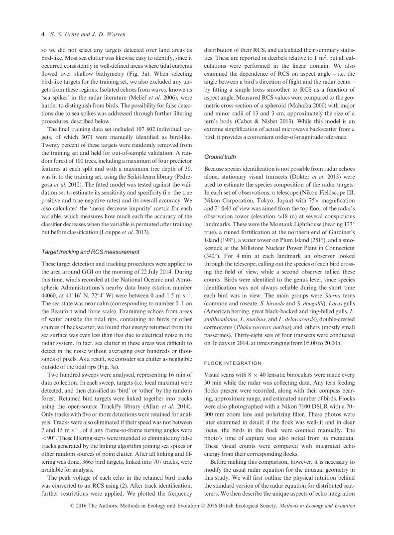
so we did not select any targets detected over land areas as

bird-like. Most sea clutter was likewise easy to identify, since it

occurred consistently in well-defined areas where tidal currents

flowed over shallow bathymetry (Fig. 3a). When selecting

bird-like targets for the training set, we also excluded any tar-

gets from these regions. Isolated echoes from waves, known as

‘sea spikes’ in the radar literature (Melief et al. 2006), were

harder to distinguish from birds. The possibility for false detec-

tions due to sea spikes was addressed through further filtering

procedures, described below.

The final training data set included 107 602 individual tar-

gets, of which 3071 were manually identified as bird-like.

Twenty percent of these targets were randomly removed from

the training set and held for out-of-sample validation. A ran-

dom forest of 100 trees, including amaximumof four predictor

features at each split and with a maximum tree depth of 30,

was fit to the training set, using the Scikit-learn library (Pedre-

gosa et al. 2012). The fitted model was tested against the vali-

dation set to estimate its sensitivity and specificity (i.e. the true

positive and true negative rates) and its overall accuracy. We

also calculated the ‘mean decrease impurity’ metric for each

variable, which measures how much each the accuracy of the

classifier decreases when the variable is permuted after training

but before classification (Louppe et al. 2013).

Target tracking andRCSmeasurement

These target detection and tracking procedures were applied to

the area around GGI on the morning of 22 July 2014. During

this time, winds recorded at the National Oceanic and Atmo-

spheric Administrations’s nearby data buoy (station number

44060, at 41�160 N, 72�40 W) were between 0 and 1�5 m s�1.

The sea state was near calm (corresponding to number 0–1 onthe Beaufort wind force scale). Examining echoes from areas

of water outside the tidal rips, containing no birds or other

sources of backscatter, we found that energy returned from the

sea surface was even less than that due to electrical noise in the

radar system. In fact, sea clutter in these areas was difficult to

detect in the noise without averaging over hundreds or thou-

sands of pixels. As a result, we consider sea clutter as negligible

outside of the tidal rips (Fig. 3a).

Two hundred sweeps were analysed, representing 16 min of

data collection. In each sweep, targets (i.e. local maxima) were

detected, and then classified as ‘bird’ or ‘other’ by the random

forest. Retained bird targets were linked together into tracks

using the open-source TrackPy library (Allan et al. 2014).

Only tracks with five ormore detections were retained for anal-

ysis. Tracks were also eliminated if their speedwas not between

7 and 15 m s�1, of if any frame-to-frame turning angles were

\90�. These filtering steps were intended to eliminate any false

tracks generated by the linking algorithm joining sea spikes or

other random sources of point clutter. After all linking and fil-

tering was done, 3665 bird targets, linked into 707 tracks, were

available for analysis.

The peak voltage of each echo in the retained bird tracks

was converted to an RCS using (2). After track identification,

further restrictions were applied. We plotted the frequency

distribution of their RCS, and calculated their summary statis-

tics. These are reported in decibels relative to 1 m2, but all cal-

culations were performed in the linear domain. We also

examined the dependence of RCS on aspect angle – i.e. the

angle between a bird’s direction of flight and the radar beam –by fitting a simple loess smoother to RCS as a function of

aspect angle.Measured RCS values were compared to the geo-

metric cross-section of a spheroid (Mahafza 2000) with major

and minor radii of 13 and 3 cm, approximately the size of a

tern’s body (Cabot & Nisbet 2013). While this model is an

extreme simplification of actual microwave backscatter from a

bird, it provides a convenient order-of-magnitude reference.

Ground truth

Because species identification is not possible from radar echoes

alone, stationary visual transects (Dokter et al. 2013) were

used to estimate the species composition of the radar targets.

In each set of observations, a telescope (Nikon Fieldscope III,

Nikon Corporation, Tokyo, Japan) with 759 magnification

and 2� field of view was aimed from the top floor of the radar’s

observation tower (elevation �18 m) at several conspicuous

landmarks. These were theMontauk Lighthouse (bearing 123�

true), a ruined fortification at the northern end of Gardiner’s

Island (198�), a water tower on Plum Island (251�), and a smo-

kestack at the Millstone Nuclear Power Plant in Connecticut

(342�). For 4 min at each landmark an observer looked

through the telescope, calling out the species of each bird cross-

ing the field of view, while a second observer tallied these

counts. Birds were identified to the genus level, since species

identification was not always reliable during the short time

each bird was in view. The main groups were Sterna terns

(common and roseate, S. hirundo and S. dougallii), Larus gulls

(American herring, great black-backed and ring-billed gulls,L.

smithsonianus,L.marinus, andL. delawarensis), double-crested

cormorants (Phalacrocorax auritus) and others (mostly small

passerines). Thirty-eight sets of four transects were conducted

on 16 days in 2014, at times ranging from 05.00 to 20.00h.

FLOCK INTEGRATION

Visual scans with 8 9 40 lensatic binoculars were made every

30 min while the radar was collecting data. Any tern feeding

flocks present were recorded, along with their compass bear-

ing, approximate range, and estimated number of birds. Flocks

were also photographed with a Nikon 7100 DSLR with a 70–300 mm zoom lens and polarizing filter. These photos were

later examined in detail; if the flock was well-lit and in clear

focus, the birds in the flock were counted manually. The

photo’s time of capture was also noted from its metadata.

These visual counts were compared with integrated echo

energy from their corresponding flocks.

Before making this comparison, however, it is necessary to

modify the usual radar equation for the unusual geometry in

this study. We will first outline the physical intuition behind

the standard version of the radar equation for distributed scat-

terers. We then describe the unique aspects of echo integration

© 2016 The Authors. Methods in Ecology and Evolution © 2016 British Ecological Society, Methods in Ecology and Evolution

4 S. S. Urmy and J. D. Warren

for tern flocks, and show how they require a modified radar

equation to account for them.

Standard radar equation for distributed targets

When there are multiple scatterers in a single pulse volume, the

total measured reflectivity at that range is equal to the total

number of scatterersNmultiplied by their meanRCS, ⟨r⟩.

Pr ¼ PTxNhriGr4

: eqn 3

The number of scatterers is in turn the product of their numeri-

cal density n (number per m3) and the pulse volume, V (m�3).

If the radar has horizontal and vertical beam widths of h and

/, the pulse volume is given by

V ¼ cspr2 sinh2

� �sin

/2

� �; eqn 4

where c and s are the speed of light (in m s�1) and the pulse

length (in s). Using the fact thatN = nV, we can rewrite Equa-

tion 3 in terms of the numerical density of birds as

Pr ¼ PTxncspr2 sinðh=2Þ sinð/=2ÞhriGr4

¼ PTxnhriG0

r2;

where the constant factors from (4) have been incorporated

into a new constant G0. Intuitively, the energy losses due to

two-way geometrical spreading still scale as r�4, but the num-

ber of birds (and hence reflectivity) increases proportional to

r2. The partial cancellation of these two scaling relations leaves

r2 in the denominator.

Modified radar equation

For the present purpose, however, a different version of the

radar equation is necessary. Feeding flocks, depending on the

number of terns, are on the order of 10s to 100s of meters

across. However, feeding terns rarely fly higher than about 6 m

above the surface (Cabot & Nisbet 2013). Because the radar

beam is vertically fan-shaped, feeding flocks will fill it horizon-

tally, but not vertically. As a result, while the pulse volume still

increases / r2 due to vertical and horizontal spreading, the

illuminated volume of the flock, Vflock, only increases in one

direction, horizontally. As a result, the number of birds illumi-

nated is

N ¼ nVflock ¼ ncs�hr sinh2

� �; eqn 5

where �h is the average height of the flock. Substituting (5) into

(3), we arrive at the correct (if unusual) radar equation for this

geometry, with a factor of r3 in the denominator,

Pr ¼ PTxnhriGr3

; eqn 6

where, once again, all constants have been gathered together

intoG for simplicity.

Integration and regression

The radar reflections from each photographed flock were out-

lined by hand using a lasso tool in a custom Python script. The

mean volume reflectivity inside each outline was multiplied by

the total outlined area to give an integral over this area. The

five radar sweeps recorded closest in time to each photo were

integrated and averaged together. Only flocks whose echoes

could be clearly separated from sea clutter and other targets

such as boats were used. Integrated echo energy was regressed

on the number of birds counted in the corresponding flock.

The slope of this line is expected to equal the average RCS of a

single bird, ⟨r⟩ (Diehl, Larkin & Black 2003). Based on the

diagnostics run on a preliminary ordinary least-squares regres-

sion, several of the data points had outsized influence (Cook’s

distance >n/4). To ensure the reliability of our results, we fit themodel, using robust regression (iterated re-weighted least

squares), as implemented in the R function ‘rlm’ in the ‘MASS’

package (Venables & Ripley 2002). The scripts used for this

analysis, and all other analyses described here, are available in

the online Supporting Information for this article (Data S1).

Results

Echoes from the calibration sphere at different ranges were

well described (R2 ¼ 0�85) by the theoretical curve (Equation2). The optimized values (�95% confidence interval) of a and

Gwere 0�0126 (�0�0003) V dB�1 and 144�7 (�2�1) dB (Fig. 2).

Though the parameters were fairly well constrained, the likeli-

hood surface showed an inverse relationship between them,

V = a(PdB − 40log10R + TS + G)

a = 0·0129 G = 145

0·6

0·8

1·0

1·2

1·4

1·6

0 100 200 300 400

Range (m)

Ech

o pe

ak (

V)

(a)

130

140

150

160

170

0·010 0·011 0·012 0·013 0·014 0·015 0·016

a (V dB−1)

G (

dB)

−2000

−1500

−1000

−500

0Δ LL

(b)

Fig. 2. Results of radar calibration. (a) Peak

voltages of echoes from the 20�3 cm diameter

stainless steel calibration sphere were well

described by the theoretical model. Line shows

predicted voltage at optimum values of the

parameters a (V dB�1) andG (dB). (b) D Log-

likelihood surface near the optimal values of

the parameters (black diamond). The surface

is normalized so the value at the maximum is

zero. Contours are drawn at �3, �10 and

�100.

© 2016 The Authors. Methods in Ecology and Evolution © 2016 British Ecological Society, Methods in Ecology and Evolution

Quantitative ornithology with a marine radar 5

indicating that the two parameters could trade off against each

other. The echoes were also variable in amplitude, with a resid-

ual standard deviation of 0�06 V. The variability in the echoes

appeared greatest at the longest ranges.

When tested against the validation data set (n = 21 521), the

random forest correctly rejected 20 861 of 20 929 non-bird tar-

gets, for a specificity of 99�7%, and detected 423 of 529 bird-

like targets, for a sensitivity of 71% (Fig. 3). The overall accu-

racy (correct/total classifications) was 99�99%. The most

important features for classification in the random forest were

mean echo level, azimuth angle, 90th percentile of echo level,

and eccentricity (Table 1). When features were correlated (e.g.

mean echo level, echo peak, and RCS), the random forest

tended to rely on them roughly evenly, as seen in their similar

importance weights.

The RCS of birds tracked on the radar ranged from �60 to

�6 dBsm, with an overall mean and median of �25 and

�34 dBsm (Fig. 4). In linear terms, these correspond to cross-

sections of 32 and 4 cm2. RCSwas 3–4 dB higher at broadside

incidence than head- or tail-on (Fig. 4a), though this wasminor

Fig. 3. Detection, classification, and tracking of bird targets from radar images. (a) Radar image showing Great Gull Island (GGI, bright patch at

centre), Little Gull Island (LGI, smaller patch to the northeast of GGI), sea clutter due to rough water in tidal rips (areas of diffuse scattering along

diagonal line from SW to NE), and terns departing GGI. The radius of the displayed image is 1�6 km. (b) Same image, with all automatically

detected local maxima marked by white points. Many of these detections are spurious (i.e. not birds), especially over land, over tidal rips, and at

longer ranges, where the signal-to-noise ratio begins to fall. (c) Same image, but with estimated non-bird targets removed by a random-forest classi-

fier. Note the rejection of almost all targets associated with areas of land and sea clutter. (d) Final set of bird tracks from this area during the sampled

time period (c. 16 min).Most are flying towards or away from the colony, consistent with the behaviour of foraging terns.

© 2016 The Authors. Methods in Ecology and Evolution © 2016 British Ecological Society, Methods in Ecology and Evolution

6 S. S. Urmy and J. D. Warren

effect: the loess model explained only 1% of the overall vari-

ance. Most birds were flying towards or away from GGI, so

aspect angles near 0� and 180� (head-on and tail-on) weremost

common. The geometric cross-section of the tern-sized ellip-

soid was greatest at broadside incidence and lowest end-on

(�12 and �38 dBsm). Birds identified in visual transects were

overwhelmingly terns: out of 5563 total birds counted, 5394, or

97%, were terns. Of the remainder, 86 were gulls, 72 were cor-

morants, and 11were other species.

Sixteen flocks had sufficiently clear photographic and radar

images to be counted and integrated. Integrated flock reflectiv-

ity was positively related to the number of birds (Fig. 5). The

slope of the regression line was 6�2 � 104 m2 per bird with a

standard error of 0�1� 10�5 m2 per bird. This corresponds to

a logarithmic RCS of �32 dBsm, or 6 cm2. The difference of

this slope from zero was highly significant (P 0�001). Thefitted intercept, 6�6 � 10�3, was not significantly different

from zero (P = 0�77).

Discussion

The theoretical calibration curve fit the raw echoes from the

calibration sphere well. As an aside, theMie-series solution for

the sphere’s RCS was within 1% of its simple geometric cross-

section (i.e. pr2), so this approximation would have been ade-

quate in this situation, with the sphere’s circumference more

than 20 times the wavelength. The estimates of the two calibra-

tion parameters were fairly well constrained, with coefficients

of variation (i.e. standard error/fitted value) both near 1%.

However, the variable voltage of the raw echoes, especially at

long ranges, limited the final accuracy of the calibration. The

maximum-likelihood values of the two parameters were nega-

tively related, indicating a minor degree of indeterminacy: an

increase in the value of one parameter could be partly offset by

a decrease in the other. Based on the precision of the estimate

of the gainG, RCSmeasurements made with this radar system

had a 95% confidence interval of c.�2 dB. It is worth empha-

sizing that these calibration values are only valid for this instru-

ment, and would have to be determined independently for

other radars. They might also be expected to shift over time as

the radar’smagnetron ages.

The uncertainty in the calibration parameters is due the vari-

able peak voltages of the raw echoes from the calibration

sphere. A certain amount of variability in the radar’s video sig-

nal was due to electrical noise. This radar was designed for reli-

able performance in a shipboard environment at reasonable

cost, not for precise reflectivity measurements, so some of the

electrical noise in the system is probably a result of the radar’s

original design goals and compromises. Also, the gasoline

Table 1. Relative importance of features included in random forest

classifier for bird targets

Feature Importance

Mean 0�18Azimuth 0�1390th percentile 0�11Eccentricity 0�11Echo peak 0�10RCS 0�08Range 0�07Size 0�06SD 0�05Median 0�0510th percentile 0�05

Features were extracted automatically from local maxima on radar

images. Importance weights are rounded for display and so do not sum

exactly to 1. RCS, radar cross-sections.

Fig. 4. Empirical tern radar cross sections

(RCS). (a) All RCS values from tern tracks

plotted as a function of their angle relative to

the radar beam. At 0�, birds are flying towardsthe radar; at 90�, they are broadside to the

beam; and at 180�, they are flying away. The

solid line shows the geometric cross-section of

a spheroid the approximate size of a tern’s

body, while the dotted line shows a fitted loess

smoother. (b) Marginal histogram of RCS

values.

0·0

0·1

0·2

0·3

0 100 200 300

Flock size (birds)

RC

S(m

2 )

Fig. 5. Integrated flock echo vs. number of birds counted in pho-

tographs. Points andwhiskers showmeans and ranges of five replicated

integrals of each flock. The regression has a y-intercept of 0 and a slope

of 6�2 � 10�4; the shaded area indicates the 95% confidence interval

for the slope.

© 2016 The Authors. Methods in Ecology and Evolution © 2016 British Ecological Society, Methods in Ecology and Evolution

Quantitative ornithology with a marine radar 7

generator, while practical on an island with no outside power

supply, was not as electrically quiet as a direct current, or a bet-

ter-filtered alternating current, system could have been.

The higher variance in echo voltage at longer ranges is

harder to explain, since electrical noise should be constant at

all ranges. One possibility is that the sphere was near the verti-

cal ‘shoulder’ of the beam’s main lobe at these locations, and

slight changes in its position caused variability in the effective

gain from the beam pattern. However, this effect was proba-

bly not major, given the beam’s 22� vertical width and the fact

that the sphere was always within a few degrees of the beam’s

centre (the geometry of the radar’s beam is discussed more in

detail below). Another possibility is a change in temperature.

On the afternoon of 17 August 2014, when measurements

were made at the two longest ranges, ambient temperatures

were near 25 �C, at least 5� higher than on any of the other

calibration dates, and the temperature inside the radar scan-

ner, in exposed sunlight, may have been higher. Thermal noise

in a conductor is proportional to temperature (Nyquist 1928),

and this temperature difference could possibly account for

higher noise in the longest-range measurements. Another pos-

sibility is that the radar beam’s side lobes may have transmit-

ted or collected returns from objects off-axis, possibly

contributing to the variability.

The random forest classifier had a much higher specificity

(99�9%) than sensitivity (71%). Put differently, these numbers

imply ‘type I’ and ‘type II’ error rates of <0�001 and 0�29. Inother words, it was highly conservative, and passed very few

false targets into the analytic sample. When combined with the

additional filtering performed by the target tracking algorithm,

in particular the rejection of short tracks and thosewith unreal-

istic speeds for terns, we can be even more confident that the

large majority of tracked targets were birds. Finally, nearly all

the birds observed visually near GGI were terns, supporting

the assumption that all bird-like targets were due to terns. This

conclusion is corroborated by the fact that most of the tracks

were flying along paths to and from the island (Fig. 3d), consis-

tent with behaviour by foraging terns. While there are proba-

bly a few returns from other species, and false detections due to

sea clutter or external noise, they are not expected to affect the

overall picture of ternRCS.

We intentionally selected a period with low winds and flat

water to measure tern RCS. The performance of our algo-

rithms, both in terms of sensitivity and specificity, would be

expected to drop during rougher conditions, when energy scat-

tered by the sea surface would overwhelm echoes from birds.

Our goal in this study was to obtain the best possible measure-

ments of tern RCS. For this reason, we only used data from a

calm period. Assessing the performance of the target detection,

classification, and tracking methods under varying conditions

of wind and sea state is an important objective on its own, and

will be the topic of a future study using this data set.

Empirical RCS values for tracked terns fell in the expected

range for birds of their size (Vaughn 1985). RCS was highly

variable, ranging across nearly five orders of magnitude,

though this is expected for radar targets with complex shapes

which change as they flap their wings (Shaefer 1968; Vaughn

1985; Chilson et al. 2012). Terns have a wingbeat frequency

on the order of 1 Hz, which is much lower than the radar’s

PRF (2100 Hz) and higher than its sweep frequency (0�2 Hz),

meaning that our RCS measurements should be approxi-

mately independent snapshots of the birds’ wingbeat cycles.

Measured RCS values were in reasonable agreement with the

range of values predicted by the simple geometric model,

though there was only a weak dependence of RCS on aspect

angle. Birds are generally expected to scatter more strongly

near broadside (Shaefer 1968), but this trend was evidently

masked by other sources of error. These could include vari-

ability in the birds’ tilt angle (which the radar could not mea-

sure), system noise in the radar, and imprecision in estimates

of the birds’ flight direction. Wind drift could also lead to

track headings that differed from the birds’ true orientation.

Finally, it is important to note that all RCS values here are

for horizontally polarized radiation, and would be expected

to change under alternate polarizations.

Total flock RCS was related linearly to the number of birds

in each flock. The slope of this line, an independent estimate of

mean tern RCS, was near the centre of the distribution mea-

sured from individual terns. Flocks displayed substantial vari-

ability in their integrated RCS from one radar image to the

next. This variability could be due to several factors. The echo

from multiple scatterers at the same range is the sum of their

individual echoes, which may interfere constructively or

destructively depending on their positions in space. This is why

it is necessary to average several successive echoes to estimate

the flock’s total RCS. Birds could also leave or join the flock in

between radar sweeps, changing the total number. Finally, the

average orientation of birds could change from one sweep to

the next, altering the mean RCS without changing the number

of birds. Regardless of the cause or causes of within-flock vari-

ability, the slope of the fitted regression line was in agreement

with the individual RCS measurements, indicating that echo

integration with a marine radar is a viable method to estimate

the number of seabirds in a near-surface feeding flock.

One aspect of the radar system we ignored in this work was

its beam pattern. In general, the energy returned from a target

depends on its angular distance from the centre of the beam.

The horizontal beam pattern could be safely ignored, since the

high PRImeant each target was ‘painted’ with at least 16 pulses

(PRF 9 rotation period 9 horizontal beam width/360�),ensuring one pulse would land on-axis, or very near it. The

effects of vertical position in the beam pattern were also likely

minor, though for different reasons. Foraging terns habitually

fly close to the water, rarely rising more than 5–10 m above the

surface. If the radar is at height h1 and a tern is flying at range

R and height h2, then its off-axis angle is tan�1ððh1 � h2Þ=RÞ.At ranges longer than a few hundred meters, this means that

nearly all terns will be within 1–2� of the beam’s vertical axis.

Since the beam is so wide vertically, the beam pattern is quite

flat on axis, so this will be a minor source of error in most of

the surveyed area. For the RCS measurements reported here,

90% of which come from ranges of 300 m or more, the effect is

negligible. Closer to the radar, however, the beam pattern

would have to be taken into account.

© 2016 The Authors. Methods in Ecology and Evolution © 2016 British Ecological Society, Methods in Ecology and Evolution

8 S. S. Urmy and J. D. Warren

The shape of the radar’s pulse was also largely ignored

in this study. As mentioned previously, the pulse generated

by the magnetron is not square, ramping up and down

from its peak transmit power over tens of nanoseconds.

We also over-sampled the video signal with respect to the

nominal range resolution. The combination of these factors

meant that each bird target typically returned some energy

in each of 4–6 consecutive range bins, with its highest

return (used to calculate RCS) in one of the central bins.

Temporal oversampling had a similar effect to painting the

target with multiple pulses: at least one digitization bin

was likely close to the true peak echo. Oversampling was

not as great in range as it was in azimuth, however, and

so the uncertainty as to where exactly the target fell in the

range gate is another source of uncertainty both in the cal-

ibration and in measuring RCS. While oversampling in

range and azimuth reduces uncertainty in RCS measure-

ments, it also increases the data storage and processing

requirements dramatically. These tradeoffs need to be con-

sidered when planning studies that depend on measuring

RCS precisely.

If birds are flying overhead, measuring their RCS

becomes much more challenging, since their position in the

beam is hard to determine. Phased array radars are cap-

able of measuring the target’s position electronically, but

have historically been too expensive for all but military

applications. However, phased array systems based on less-

expensive solid-state amplifiers are beginning to be used in

meteorological research. There is a possibility that they will

become available to radar biologists as well at some point

in the not-too-distant future.

This paper demonstrates a practical method tomakemarine

radar measurements truly quantitative by calibrating the radar

with a standard target. The procedure is straightforward and

does not require a great deal of time. Field calibration can be

performed in a few hours or less, and the analysis required is

no more complex than fitting a nonlinear regression model.

The benefits are considerable – even with an off-the-shelf mar-

ine radar, empirical RCS measurements can be taken, and the

size of flocks estimated accurately from their integrated

echoes.

The last major review of RCS in radar biology (Vaughn

1985) is over 30 years old. The physics of radar scattering

from biological targets is poorly understood, and most

models to date have been based on simple shapes like

sphere, cylinders, and spheroids. To our knowledge only

one group has calculated scattering from a bird model

with realistic shape and material properties (Torvik et al.

2014). More theoretical and modelling work is clearly

needed, as are field measurements of as many species as

possible. Accurate RCS values are needed to estimate the

density of animals in distributed bioscatter, for instance in

large-scale studies of bird migration, using weather radars.

And knowledge of the scattering properties of individual

organisms is the first step on the difficult path to remotely

classifying them. Before one can obtain these necessary

data, calibration is the necessary procedure.

Authors’ contributions

S.S.U. conceived and designed the study, collected and analysed the data,

and drafted the manuscript. J.D.W. provided guidance on methodology and

analysis. Both authors edited the manuscript and approved it for publica-

tion.

Acknowledgements

We are grateful to Dr. Helen Hays of the AMNH and Great Gull Island Project

for allowing us to work on GGI, and to the many other volunteers and scientists

on who made that work such a pleasure. This project would not have been possi-

ble without the capable field assistance of Maria Anderson and Emily Runnells.

The StonyBrook Southampton PoliceDepartmentwere very understanding dur-

ing the late-night parking lot calibrations. Allan Reynolds of Port Neches, TX

generously exchanged needed radar parts for beer and fishing lures. We also

thank Dr. Ron Larkin and three anonymous referees for their helpful comments.

Funding for this work was provided by the FrankM. ChapmanMemorial Fund

of theAMNH.We declare no conflicts of interest.

Data accessibility

Processed data and analysis scripts inR andPython have been uploaded as online

Supporting Information.Raw radar data has been deposited in theDryadRepos-

itory: http://datadryad.org/resource/doi:10.5061/dryad.45gb4 (Urmy & Warren

2016). The Python script used to digitize the radar data using the oscilloscope is

available online at https://github.com/ElOceanografo/PyRad/blob/master/src/

radar_scope.py.

References

Allan, D., Caswell, T.A., Keim,N., Boulogne, F., Perry, R.W.&Uieda, L. (2014)

TrackPy v0.2.4. Available at: https://github.com/soft-matter/trackpy [accessed

15November 2016].

Atlas, D. (2002) Radar calibration: some simple approaches.Bulletin of the Amer-

icanMeteorological Society, 83, 1313–1316.Breiman, L. (2001) Random forests.Machine Learning, 45, 5–32.Bruderer, B. (1997) The study of bird migration by radar. Naturwissenschaften,

84 (2): 45–54.Burger, A.E. (2001) Using radar to estimate populations and assess habitat

associations of Marbled Murrelets. The Journal of Wildlife Management, 65,

696–715.Cabot, D.&Nisbet, I. (2013)Terns. Collins, London,UK.

Chilson, P.B., Frick, W.F., Kelly, J.F., Howard, K.W., Larkin, R.P., Diehl,

R.H., Westbrook, J.K., Kelly, T.A. & Kunz, T.H. (2012) Partly cloudy with a

chance of migration: weather, radars, and aeroecology. Bulletin of the Ameri-

canMeteorological Society, 93, 669–686.Coelho, L.P. (2013) Mahotas: open source software for scriptable computer

vision. Journal of Open Research Software, 1(July), 1–7. doi: 10.5334/

jors.ac.

Desholm, M., Fox, A., Beasley, P., & Kahlert, J. (2006) Remote techniques for

counting and estimating the number of bird–wind turbine collisions at sea: a

review. Ibis, 148, 76–89.Diehl, R.H., Larkin, R.P. & Black, J.E. (2003) Radar observations of bird migra-

tionover the great lakes.TheAuk, 120, 278–290.Dokter, A.M., Baptist, M.J., Ens, B.J., Krijgsveld, K.L. & van Loon, E.E. (2013)

Bird radar validation in the field by time-referencing line-transect surveys.PloS

One, 8, e74129.

Eastwood, E. (1967)Radar Ornithology.Metheuen Books, London.

Ho, T.K. (1995) Random decision forests. Proceedings of the 3rd International

Conference on Document Analysis and Recognition vol 1, pp. 278–282. IEEE,Montreal.

Jones, E., Oliphant, T., Peterson, P. et al. (2001) SciPy: Open source scientific

tools for Python. Available at: http://www.scipy.org/ [accessed 11 November

2016].

Larkin, R.P. & Diehl, R.H. (2012) Radar techniques for wildlife research. The

Wildlife Techniques Manual, chapter 13, 7th edn (ed. N.J. Silvy), pp. 319–340.JohnsHopkinsUniversity Press, Baltimore,MD.

Louppe,G.,Wehenkel, L., Sutera,A.&Geurts, P. (2013)Understanding variable

importances in forests of randomized trees. Advances in Neural Information

Processing Systems, 26, 431–439.Mahafza, B.R. (2000) Radar cross section (RCS). Radar Systems Analysis and

Design using MATLAB, chapter 14, pp. 485–540. Chapman Hall/CRC, Boca

Raton, FL,USA.

© 2016 The Authors. Methods in Ecology and Evolution © 2016 British Ecological Society, Methods in Ecology and Evolution

Quantitative ornithology with a marine radar 9

Melief, H.W., Greidanus, H., VanGenderen, P. &Hoogeboom, P. (2006) Analy-

sis of sea spikes in radar sea clutter data. IEEE Transactions on Geoscience and

Remote Sensing, 44, 985–993.Nohara, T.J., Weber, P., Premji, A., Krasnor, C., Gauthreaux, S.A., Brand, M.,

& Key, G. (2005) Affordable avian radar surveillance systems for natural

resourcemanagement andBASHapplications. IEEE International Radar Con-

ference, 2005, vol 1, pp. 10–15, IEEE,Arlington, VA.Nohara, T.J., Eng, B., Eng, M., Weber, P., Ukrainec, A. & Jones, G. (2007) An

overview of avian radar developments–past, present and future. Bird Strike

2007Conference, pp. 1–8,Kingston, Ontario, Canada.

Nyquist, H. (1928) Thermal agitation of electric charge in conductors. Physical

Review, 32, 110–113.Pedregosa, F., Varoquaux, G., Gramfort, A.et al. (2012) Scikit-learn:

machine learning in Python. Journal of Machine Learning Research, 12,

2825–2830.R Development Core Team. (2014) R: A language and environment for statistical

computing. R Foundation for Statistical Computing, Vienna. Available at:

http://www.r-project.org [accessed 11November 2016].

Rosa, I.M.D., Marques, A.T., Palminha, G., Costa, H., Mascarenhas, M., Fon-

seca, C. & Bernardino, J. (2016) Classification success of six machine learning

algorithms in radar ornithology. Ibis, 158, 28–42.Safavian, S.R. & Landgrebe, D. (1990) A survey of decision tree classifier

methodology. IEEE Transactions on Systems, Man, And Cybernetics, 21, 660–674.

Shaefer, G.W. (1968) Bird recognition by radar: a study in quantitative radar

ornithology. The Problems of Birds as Pests: Institute of Biology Symposia

Number 17 (eds R. Murton and E. Wright), pp. 53–86, Academic Press, New

York,NY,USA.

Shamoun-Baranes, J., Alves, J.A., Bauer, S.et al. (2014) Continental-scale radar

monitoring of the aerial movements of animals.Movement Ecology, 2, 9.

Stepanian, P.M., Chilson, P.B. & Kelly, J.F. (2014) An introduction to radar

image processing in ecology.Methods in Ecology and Evolution, 5, 730–738.Torvik, B., Knapskog, A., Lie-Svendsen, Ø., Olsen, K.E. &Griffiths, H.D. (2014)

Amplitudemodulation on echoes from large birds.EuropeanMicrowaveWeek

2014: ‘Connecting the Future’, EuMW2014 –Conference Proceedings; EuRAD2014: 11th EuropeanRadar Conference, pp. 177–180.

Urmy, S.S. &Warren, J. (2016) Data from: Quantitative ornithology with a com-

mercial marine radar: standard-target calibration, target detection and track-

ing, and measurement of echoes from individuals and flocks. Dryad Digital

Repository, http://dx.doi.org/10.5061/dryad.45gb4

Vaughn, C.R. (1985) Birds and insects as radar targets: a review. Proceedings of

the IEEE, 73, 205–227.Venables, W.N. & Ripley, B.D. (2002)Modern Applied Statistics with S, 4th edn.

Springer, NewYork, NY,USA.

Received 6 July 2016; accepted 20October 2016

Handling Editor: Francesca Parrini

Supporting Information

Additional Supporting Information may be found online in the support-

ing information tab for this article:

Data S1.Analysis scripts.

© 2016 The Authors. Methods in Ecology and Evolution © 2016 British Ecological Society, Methods in Ecology and Evolution

10 S. S. Urmy and J. D. Warren