Quantitative Risk Tolerance Analysis and Simulation ...
103
Quantitative Risk Tolerance Analysis and Simulation Template Development by Xiang Yu Zhou A thesis submitted in partial fulfillment of the requirements for the degree of Master of Science In Construction Engineering and Management Department of Civil and Environmental Engineering University of Alberta © Xiang Yu Zhou, 2015
Transcript of Quantitative Risk Tolerance Analysis and Simulation ...

Quantitative Risk Tolerance Analysis and Simulation Template Development
by
Xiang Yu Zhou
A thesis submitted in partial fulfillment of the requirements for the degree of
Master of Science
In
Construction Engineering and Management
Department of Civil and Environmental Engineering University of Alberta
© Xiang Yu Zhou, 2015

ii
Abstract
In the current construction industry, simulation is an effective technology that can assist
engineers’ decision making on project planning and estimation. The key contribution of
simulation is to model uncertainty and risk occurrence during the construction process;
however, this method still lacks a quantitative method to determine how much risk the
decision maker is willing to accept. This thesis aims to develop an approach that can assist
decision making on what percentile from a cumulative distribution function (CDF) of project
cost reflects the organization’s risk appetite and overall acceptance of risk. In order to
enhance this quantitative risk analysis, a special purpose template was re-developed in
Simphony.Net, based on program evaluation and review technique (PERT). This template
provides an integrated cost/schedule model, and transforms the model to simulation-
based planning, in which the uncertainties of project cost and schedule are evaluated
through computer simulation.

iii
Table of Contents
1 Introduction .................................................................................................................. 1
1.1 Background ........................................................................................................... 1
1.2 Purpose of the Study ............................................................................................. 2
1.3 Expected Contributions .......................................................................................... 3
1.4 Research Methodology .......................................................................................... 3
1.5 Thesis Organization ............................................................................................... 4
2 Literature Review ......................................................................................................... 5
2.1 Introduction ............................................................................................................ 5
2.2 Definitions .............................................................................................................. 5
2.3 Examining an Individual’s Risk Tolerance .............................................................. 6
2.3.1 Culture ............................................................................................................ 6
2.3.2 Risk Attitude .................................................................................................... 9
2.3.3 Individual Decision Makers’ Risk Attitudes towards Construction Organizations
............................................................................................................................... 12
2.4 Examining Organization’s Risk Tolerance ............................................................ 13
2.4.1 Risk Identification .......................................................................................... 14
2.4.2 Quantitative Risk Analysis ............................................................................. 17
2.4.3 Organization’s Risk Appetite.......................................................................... 18
2.5 Literature Limitation ............................................................................................. 21
3 Determining Risk Tolerance: Utility Theory ................................................................. 22
3.1 Introduction of Utility Theory ................................................................................ 22
3.2 Expected Value .................................................................................................... 22
3.3 Expected Utility .................................................................................................... 24
3.3.1 Expected Utility Curve ................................................................................... 27
3.3.2 Create Utility Function ................................................................................... 31
3.3.3 Common Types of Utility Functions ............................................................... 35
4 Application of Utility Theory ........................................................................................ 42
4.1 Determine the Utility Curve for a Cumulative Project Cost ................................... 42
4.1.1 Risk Capacity ................................................................................................ 42
4.1.2 Create Utility Curve ....................................................................................... 44
4.2.1 Determine the Shape of the Risk Utility Function ........................................... 49
4.3 Two Utility Function Combination ......................................................................... 49
4.3.1 Utility Function Normalization ........................................................................ 50

iv
4.3.2 Overall Utility Formation ................................................................................ 52
4.3.3 Determine the Weight of Utility Function ........................................................ 55
5 Development of Simulation Tool ................................................................................. 58
5.1 Framework of PERT ............................................................................................ 58
5.1.1 WBS .............................................................................................................. 58
5.1.2 Basic Theory of PERT ................................................................................... 61
5.1.3 PERT Network Diagram ................................................................................ 62
5.2 Original PERT Template in Simphony.NET .......................................................... 64
5.2.1 Structure of Original PERT Template ............................................................ 64
5.2.2 Limitations of Original Template .................................................................... 67
5.3 Revised PERT Template Interface ....................................................................... 68
5.3.1 Modeling Elements of PERT Template .......................................................... 68
5.3.2 Input and Output Data Processing ................................................................. 71
6 Case Study................................................................................................................. 75
6.1 Project Information ............................................................................................... 75
6.2 Create Simulation Model in PERT ........................................................................ 76
6.3 PERT Template Output ........................................................................................ 81
6.3 Determine Organization’s Risk Appetite ............................................................... 87
7 Conclusion ................................................................................................................. 92
7.1 Conclusion ........................................................................................................... 92
7.2 Limitations and Future Recommendations ........................................................... 93
References .................................................................................................................... 94

v
List of Figures
Figure 1 Sample risk matrix ........................................................................................... 21
Figure 2 The expected utility for the game ..................................................................... 26
Figure 3 Sample utility curve for risk aversion ............................................................... 28
Figure 4 Sample utility curve for risk neutrality .............................................................. 30
Figure 5 Sample utility curve for risk seeking................................................................. 31
Figure 6 Equivalent value for risk averse, risk neutral, and risk seeking ........................ 33
Figure 7 Sample utility function for risk aversion ............................................................ 34
Figure 8 Sample utility function for risk seeking ............................................................. 35
Figure 9 What is the maximum amount (R) you would accept ....................................... 37
Figure 10 Sample exponential utility function ................................................................ 39
Figure 11 Determine the certain equivalent ................................................................... 40
Figure 12 Example of customize utility function ............................................................. 41
Figure 13 CDF plot of project cost ................................................................................. 44
Figure 14 CDF of project cost fitted by normal distribution ............................................ 45
Figure 15 Probability confidence vs. potential profit ....................................................... 47
Figure 16 Exponential utility function of potential profit .................................................. 48
Figure 17 Sample risk utility function ............................................................................. 49
Figure 18 Normalized profit utility curve ......................................................................... 51
Figure 19 Profit utility function with respect to project cost............................................. 53
Figure 20 Project risk utility function with respect to project cost ................................... 53
Figure 21 Overall utility function R=10000 ..................................................................... 54
Figure 22 Overall utility function R=30000 ..................................................................... 55
Figure 23 Overall utility curve with applied weight coefficient ........................................ 56
Figure 24 Sample WBS for house construction (Mark Swidersik, 2012) ........................ 60
Figure 25 Sample AON diagram.................................................................................... 63

vi
Figure 26 PERT scheduling ........................................................................................... 63
Figure 27 Sample WBS for PERT template ................................................................... 64
Figure 28 Resource block ............................................................................................. 65
Figure 29 Risk breakdown structure .............................................................................. 66
Figure 30 Flowchart of simulation process (Hong, 2012) ............................................... 67
Figure 31 Template elements and relationship .............................................................. 69
Figure 32 Network diagram of the revised PERT template ............................................ 70
Figure 33 Sample cost result ......................................................................................... 74
Figure 34 Project element ............................................................................................. 77
Figure 35 PERT network diagram ................................................................................. 78
Figure 36 Resource input table ..................................................................................... 79
Figure 37 Assign resource into activities ....................................................................... 80
Figure 38 Risk assignment sample ................................................................................ 81
Figure 39 CDF graph of the project completion duration ............................................... 82
Figure 40 CDF graph of the project completion cost ...................................................... 82
Figure 41 CDF curve of project cost .............................................................................. 87
Figure 42 CDF curve of project cost converted to normal distribution curve .................. 88
Figure 43 Potential gain and loss of the project ............................................................. 88
Figure 44 Utility function of potential profit ..................................................................... 89
Figure 45 Utility function of potential profit (normalized) ................................................ 90
Figure 46 Utility curve for potential risk (normalized) ..................................................... 90
Figure 47 Overall utility function .................................................................................... 91

vii
List of Tables
Table 1 Culture & Risk Tolerance (Statman, 2010) ......................................................... 7
Table 2 Risk Likelihood and its Linguistic Interpretation ................................................ 16
Table 3 Risk Verbal Expression and its Corresponding Impact ..................................... 16
Table 4 Considerations Affecting Risk Appetite (COSO, 2012) ..................................... 19
Table 5 Gamble Payoff .................................................................................................. 25
Table 6 Sample Utility of Risk Aversion ......................................................................... 27
Table 7 Sample Utility for Risk Neutrality ....................................................................... 29
Table 8 Sample Utility for Risk Seeking ......................................................................... 31
Table 9 Project Cost and Potential Profit ....................................................................... 46
Table 10 Sample Project Sequence and Duration ......................................................... 61
Table 11 WBS of the Hypothetical Road Construction (Hong, 2012) ............................. 75
Table 12 Project Cost of WBS ....................................................................................... 83
Table 14 Resource Cost Report .................................................................................... 85

1
1 Introduction
1.1 Background
A typical construction project can be categorized into five basic process groups,
which are initiating, planning, executing, monitoring and controlling, and closing (Project
Management Institute, 2004). Among them, planning is the most prominent process, and
nearly half of the processes occurring in a project fall within this group. More importantly,
a quantitative risk analysis (QRA) is usually done in this process, related to the project
management plan, scope, and activities. The objectives of the QRA are to increase the
probability and impact of positive events and decrease the probability and impact of
adverse events (PMI, 2004).
A capital construction project undergoes various risk factors including funding risk,
schedule risk, cost risk, and technical risk. Simulation is widely used as an effective risk
analysis method in the project pre-planning process to estimate the impact of those
uncertainties. This thesis focuses on quantitatively defining an organization’s risk
tolerance towards a certain project based on Monte Carlo Simulation results. The
simulation supplies the decision maker with all the possible outcomes and the probabilities
that they will occur, which is usually shown as a distribution. For example, the simulated
result of a project cost can be displayed as a cumulative distribution curve (CDF) within a
range between the lowest possible price and the maximum possible price. The Monte
Carlo method delivers a new level of project estimation process compared to the traditional
“cost plus contingency” method.
Over the past few decades, the construction industry has valued risk analysis as
one of the most significant components of project success. When it comes to
understanding risks, organizations need to focus on two dimensions of risk: investment
risks and investor risk. Investment risk encompasses the risk traits of an investment or
2
project, and investor risk lies on the head of the investor. However, how much risk an
organization is willing to accept is still debatable. Two key aspects (1) risk appetite and (2)
risk capacity are currently used to assist decision making. Risk appetite is defined as “the
amount of risk, on a broad level, an organization is willing to accept in pursuit value”
(COSO, 2012). Nowadays, many construction companies have created their own risk
appetite statements. A sample risk appetite statement can be defined as follows, “we
expect a return of 18% on this investment, we are not willing to take more than a 25%
chance that the investment leads to a loss of more than 50% of our existing capital” (COSO,
2012). Risk capacity is the amount of risk that the company can undertake. There are
multiple ways to determine risk capacity; and normally it standards for the bottom line of
a company’s risk seeking decision. For contractors, the risk capacity usually explores the
dividing line between profits and losses. For owners, the risk capacity is the budget of a
project where the profit and losses are transferred to savings to budget and exceeding of
the budget. For the rest of the thesis, the terms profits and losses are used in the new
developed approach.
Although the aforementioned two aspects are important in decision making, there
is still a lack of comprehensive methods to express a company’s overall risk tolerance.
The current recommendation for risk tolerance is at the 85th percentile of the
aforementioned CDF, which means a 15% possibility of cost overrun (SMA Consulting).
This research aims to develop an approach that can assist a decision maker to determine
a more reliable percentile from the cumulative distribution curve so that the selected price
will reflect the organization’s overall risk tolerance.
1.2 Purpose of the Study
Although risk analysis is not a new topic in the construction industry, risk tolerance
is still worthy of study because of its subjectivity. The purpose of this study was to:
Understand the QRA using Monte Carlo Simulation.

3
Provide a list of possible factors which will influence an organization’s overall risk
tolerance.
Provide a method for assisting decision makers in deciding on what percentile to
use from the cumulative distribution curve that will reflect a company’s risk
tolerance. This thesis will mainly focus on defining an organization’s acceptance
of risk of project cost overrun. .
Provide improvements to the user interface of a program evaluation and review
technique (PERT) special purpose template developed in Simphony.NET.
1.3 Expected Contributions
Develop a new approach to quantitatively assess an organization’s attitudes
towards risk, in order to help organizations to select the most comfortable project
cost.
Develop a simulation template based on PERT.
1.4 Research Methodology
This research was conducted using the following methodology:
Conduct a literature review on risk tolerance, decision making, quantitative risk
analysis, Monte Carlo method, and utility theory.
Study a company’s risk appetite and capacity in order to determine the factors
that influence an organization’s decision making.
Study utility theory related to risk tolerance decision.
Develop a method using utility theory to assist an organization to determine a
reliable risk tolerance range.
Interview professional engineers to simplify a simulation template which assists
the research.

4
1.5 Thesis Organization
The thesis is divided into seven main chapters with a list of references.
Chapter 1 outlines the research background, research objectives, methodology, and
expected contributions.
Chapter 2 contains a literature review of previous research about the risk attitude in
construction fields. The chapter also provides the gaps of the previous research.
Chapter 3 presents an introduction to utility theory and explains the conceptual idea of
using utility theory to model an organization’s or individual’s risk tolerance.
Chapter 4 explains the new approach developed for quantitative risk tolerance analysis. It
introduces the procedure of how to measure an organization’s risk tolerance using utility
theory.
Chapter 5 introduces the re-developed template.
Chapter 6 describes a hypothetical road construction project that is simulated using the
new template. It introduces the step-by-step procedure of creating a model in the related
template.
Chapter 7 includes the conclusions, limitations, and future enhancements.

5
2 Literature Review
2.1 Introduction
Akintoye and MacLeod (1997) indicate that risk in construction has been an object
of attention because of the time and cost over-runs associated with construction projects.
Since construction is a risky business, effective risk management is important because it
analyzes and controls risk as the key to profit. Quantitative risk analysis (QRA), with
respect to an organization’s risk tolerance, is a vital part of archiving risk management and
it provides more detailed information compared to traditional qualitative risk assessment.
An organization’s risk tolerance can be influenced by various categories. Kwak and
LaPlace (2004) suggest that risk tolerance related to a project consists of three
perspectives, which are firm, project manager, and stakeholder. It is so dependent on the
human dynamic that a quantitative measure of an organization or individual’s risk
tolerance is difficult to achieve. Numerous research projects have been undertaken to
examine the topic of risk management.
2.2 Definitions
There are numerous definitions of risk tolerance and risk appetite. The following is
a select set of definitions that are commonly encountered:
According to the PMBOK Guide (2013), risk tolerance is the “degree, amount or
volume of risk that an organization or individual will withstand.” If an organization
or stakeholder is willing to accept risks with high impact or high possibility of
occurrence, they are considered to have high risk tolerance.
ISO Guide 73 (2009) defines risk tolerance as an “organization’s or stakeholder’s
readiness to bear the risk after risk treatment in order to achieve its objectives,”
and risk appetite is defined as the “amount and type of risk that an organization is
willing to pursue or retain.”

6
COSO (2012) indicates that risk tolerance “reflects the acceptable variation in
outcomes related to specific performance measures linked to objectives the
entity seeks to achieve.” In COSO’s framework, risk appetite is defined as the
“amount of risk, on a broad level, an organization is willing to accept in pursuit of
value.” Each organization pursues various objectives to add value and should
broadly understand the risk it is willing to undertake in doing so. For example, a
financial organization with a lower risk appetite might choose to avoid
opportunities that are more risky, but offer greater returns.
KPMG (2009) defines risk tolerance as the “typical measures of risk used to
monitor exposure compared with the stated risk appetite,” and risk appetite is
defined as the “total impact of risk an organization is prepared to accept in the
pursuit of its strategic objectives.” The corporation indicates that the amount of
risk acceptable varies from organization to organization, and the risk appetite
also various across business units and risk types.
2.3 Examining an Individual’s Risk Tolerance
In the past few decades, individual’s risk tolerance has being examined through
multiple dimensions. Three aspects are the essential targets used to analyze an
individual’s risk tolerance:
1. Culture
2. Risk Perception
3. Risk Preference
2.3.1 Culture
The following section explores the links between culture and an individual’s risk
tolerance. Risk is associated with culture. Individuals with different cultural backgrounds

7
will have different attitude towards risk. Furthermore, risk tolerance varies depending on
gender, age, etc.
2.3.1.1 Culture Difference
Statman (2010) explores the relationship between cultural background and risk
tolerance. From his research, various factors have been discovered that can influence an
individual’s risk tolerance. Table 1 summarizes the key factors from Statman’s research
that link culture and risk tolerance.
Table 1 Culture & Risk Tolerance (Statman, 2010)
Risk Tolerance
High Low
Collectivistic Countries Individualistic Countries
Low Income-Per-Capital High Income-Per-Capital
High Social Spending High Uncertainty Avoidance
Egalitarian Countries
Harmonious Countries
Before Statman explored the correlation between culture and risk tolerance, other
research had already been conducted on the same topic. Fan and Xiao’s (2003) study on
this topic compared risk-taking attitudes and behaviors between Chinese and Americans.
The findings show that Chinese are more risk tolerant than Americans in their financial
decisions, which is similar to Statman’s statement (2010).
Hsee and Weber (1998) suggest that risk perception varies between cultures. They
indicate that those from a collective country will have a lower risk perception than those
from an individualism country, which results in a higher risk tolerance level (1998). Hsee
and Weber (1999) also prove that systematic cross-national differences in risk preference

8
exist. Their research aims to quantitatively analyze risk preferences between Americans
and Chinese and study the correlation between risk preference and risk perception. Weber
(2013) examines the correlation between personality and risk tolerance by conducting an
investigation of risk-taking behavior. The results show that people with large worries about
finances have a higher probability of being risk averse and people with virtually no worries
about finances are more likely to be risk prone.
Griffin et al. (2009) investigate the role of national culture in corporate risk-taking
using individual data at the firm level from 35 countries. Based on their research, three
factors (1) harmony, (2) individualism, and (3) uncertainty avoidance are identified from
the national culture that may impact risk-taking attitudes. The research reveals that
harmony and uncertainty avoidance are negatively associated with an individual’s risk
tolerance, but individualism is positively associated with risk tolerance.
Frijins et al. (2013) examine the role of national culture in corporate takeover
decisions to show that culture affects financial decision making at the individual level. The
research team collect a sample of 25,750 acquisitions made by 7,681 firms from 39
countries to find that countries with higher levels of religiosity and uncertainty avoidance
will have a lower risk tolerance.
Ryack (2011) explores how family relationships and financial education impact an
individual’s risk tolerance using a sample of college freshmen and their parents. The
results show that higher levels of financial education will lead to lower risk tolerance;
however, the education level of relatives has no significant impact on an individual’s risk
tolerance.
2.3.1.2 Gender Difference
Statman (2010) indicates in his research that women have lower risk tolerance
than men in both portfolios and jobs. In this, Statman is consistent with many others.
Beckmann et al. (2008) suggest that women are significantly more risk averse, tend to be

9
less overconfident and behave less competitively-oriented in the financial industry with
risk taking and decision making. Charness and Gneezy (2007) identify consistent results
that women invest less, which indicates that they tend to be more financially risk averse
than men. Watson and McNaughton (2007) suggest that women choose more
conservative investment strategies than men, which directly results in relatively lower
retirement benefits. Lemaster and Strough (2013) again indicate the gender difference
that men are more risk tolerant and make riskier financial decision than women from the
perspective of core biological mechanisms.
2.3.1.3 Age Difference
Several studies mention that risk attitudes and tolerance vary with age. Weber
(2013) classifies that as age increases, risk tolerance decreases. In addition, the research
indicates that married individuals are more likely to be risk averse, and their risk tolerance
is in a direct ratio towards their number of children. In this, Weber is consistent with other
research. Sahm (2007) explores the impact of life cycle on an individual’s risk tolerance
through a measure of a gamble test response under macroeconomic conditions. The
researcher indicates that each year of age is associated with a 1.7% decline in an
individual’s risk tolerance.
2.3.2 Risk Attitude
Despite culture factors, an organization’s leader’s attitude towards risk will have
greater impacts on decision making. Frijins et al. (2013) indicate that risk decisions are
affected by the company leader’s personal traits and interests. Their research was
conducted on a company’s takeover decisions, and the results show that a CEO’s appetite
for risk or perception of risk involved may play a decisive role.
The methods to determine an individual’s risk attitude have been examined
through research for many years. Risk attitude is composed of risk perception and risk

10
preference. Statman (2010) indicates that wealthy people may have the same risk
preference as poor people in the same situation, yet their risk perceptions are likely to be
different. The same proposition can be made on the project cost and company assets for
decision maker’s risk perception of a construction organization.
2.3.2.1 Risk Perception
Perception is an important factor to be taken into account when communicating
risks. Risk perception is usually understood as the subjective judgement that people make
about the characteristics and severity of a risk. The risk perception is generally influenced
by an individual’s beliefs, attitudes, judgements and feelings (Akintoye & MacLeod, 1997).
Solvic (2004) suggests that risks and benefits are positively correlated in real life; however,
risk perception and benefits are negatively correlated. Based on Solvic’s work, Nyre and
Jaatun (2013) constructed a multi-dimensional risk perception model to quantitatively
measure an individual’s risk perception.
2.3.2.2 Risk Preference
Risk preference is the tendency of an individual to choose a risky or less risky
option. It can be applied to any decision that involves risk. Several types of risk preference
exist, and the associated risk involved generally depends on the decision maker and for
whom the decision maker takes the risk.
Risk Preference Definition
In decision theory, risk refers to the attitude of a decision maker towards a
particular lottery (Keeney & Raiffa, 1976). Wild (2013) suggests that this risk attitude is
characterized by the preference of the decision maker either for the certain amount “z,” or
for a risky lottery “L” with expected value “z.” Based on this research, a person is
considered risk averse if he/she prefers the amount “z” to any risk lottery “L” with expected
“z,” i.e., z > L; a person is considered as risk seeking if the lottery “L” is preferred to its

11
expected value “z,” i.e., L > z; and risk neutrality means that the decision maker is
indifferent between every lottery and its expected value, i.e., z = L.
Despite the decision theory of risk averse or risk seeking, Hanna et al. (2001)
classify risk preference into 5 standard statements, as follows, which are determined
through a set of questionnaires.
1. Take substantial financial risk expecting to earn substantial returns.
2. Take above average financial risk expecting to earn above average returns.
3. Take average financial risk expecting to earn average returns.
4. Take low financial risk expecting low returns.
5. Not willing to take any financial risk.
Risk Preference Measure
Individuals’ risk preferences have been measured in a variety of ways. Gilliam et
al. (2010) concluded that two common methods to assess financial risk tolerance are (1)
single risk-tolerance item found in the survey of consumer finances (SCF), and (2) 13-item
financial risk-tolerance scale (Grable & Lytton, 1999).
Barsky et al. (1997) attempt to elicit individual preference parameters about risk
through questions derived from economic theory. The research team obtained the
measure of risk aversion by asking respondents about their willingness to gamble on
lifetime income. A sample question is shown as follows:
Suppose that you are the only income earner in the family, and you have a good
job guaranteed to give your current family income every year for life. You are
given the opportunity to take a new and equally good job, with a 50-50 chance
it will double your family income and a 50-50 chance that it will cut your family
income by a third. Would you take the new job? (Hanna 2001).
Hanna et al. (2001) indicate four effective methods of measuring risk preference.

12
1. Asking about investment choice,
2. Asking a combination of investment and subjective questions,
3. Assessing actual behavior, and
4. Asking hypothetical questions with carefully specified scenarios.
2.3.3 Individual Decision Makers’ Risk Attitudes towards Construction Organizations
“Construction, like many other industries in a free-enterprise system, has sizeable
risk built into its profit structure” (Mustafa and Al-Bahar, 1991). Although previous work
intended to examine an individual’s attitude towards risk, a decision maker’s risk attitude
towards a construction organization is still considered risk aversion.
An individual’s risk tolerance is still a debatable topic because of its human dynamic;
however, early studies found that individual decision makers are risk averse (Pratt, 1964
& Arrow, 1965). Kaheman and Lovallo (1993) suggest that project managers are
“extremely susceptible to unjustified optimism and unreasonable risk aversion.” Their
research proposes that project managers or decision makers will intuitively become
prudent risk takers themselves because of pressure from project uncertainties. Akintoye
and Macleod (1996) indicate that risk management is important to construction
organizations because of the need to limit professional indemnity and to protect
companies’ reputations. The study included several surveys of contractors on project
management practices, and the results prove that decision makers are biased towards
safer projects with lower profits as compared to risky investments. Hanna and Lindamood
(2004) indicate that decision makers usually place a lower value on gain than they place
on losses, which means that when individuals are confronted with risky investments, they
are somewhat risk averse. Hulett (2013) indicates that decision makers may shy away
from project alternatives that would expose the organization to significant down-side

13
results if they are to fail, even if these kinds of projects also offer a great opportunity of up-
side results and success.
Kwak and LaPlace (2005) argue that the pre-determined risk tolerance level is
nullified without the proper recognition of risks. The researchers suggest that project
managers should weigh the credit and blame before making any decisions. The
importance of a project will also influence a project manager’s risk tolerance. For example,
if a manager possesses a promotion chance, he or she may accept more risk in a highly
visible project to gain accolades; however, the project manager may have less incentive
to take risks in smaller projects (Kwak and LaPlace, 2005). This risk attitude is in contrast
with the firm’s risk tolerance profile because construction organizations are willing to take
risks on relatively smaller projects that have little impact on the entire company
environment.
2.4 Examining Organization’s Risk Tolerance
In order to survive in the market, organizations have developed their own risk
management processes, which are now commonly referred to as enterprise risk
management (ERM). The COSO (2004) identifies the ERM as “a process, effected by an
entity’s board of directors, management and other personnel, applied in strategy setting
and across the enterprise, designed to identify potential events that may affect the entity,
and manage risks to be within its risk appetite, to provide reasonable assurance regarding
the achievement of entity objectives.” In order to achieve effective risk management,
organizations must know how much risk is acceptable as they consider ways to
accomplish objectives, both at the organization level and individual level. ERM is often
qualitative in nature; however, this approach aims to quantitatively analyze risk appetite.
Three major steps are essential to the objective: (1) risk identification, (2) quantitative risk
analysis, and (3) develop risk appetite.

14
2.4.1 Risk Identification
Risk management is divided into four stages: risk identification, risk analysis, risk
mitigation, and risk control (AbouRizk, 2009; Abdelgawad, 2010). Among them, risk
identification is an indispensable process because insufficient or unrealistically defined
risks may mislead the management of an entire project. PMI (2000) defines risk
identification as the process of investigating risk events that might become threats or
opportunities to the projects. Huang and Wang (2008) indicate that one-off construction
projects have greater uncertainty than other activities, so that identification and
management of construction risks becomes more difficult and imperious. Perry and Hayes
(1985) and Mustafa and Al-Bahar (1991) have defined key risk sources to construction
activities, which are physical, environmental, design, financial, legal, construction and
operation risks.
2.4.1.1 Risk Factor Identification
There are multiple ways to identify risk factors for a construction project. Huang
and Wang (2008) indicate five common methods for construction project risk assessment,
which are: (1) investigation and expert marking method, (2) fuzzy mathematics, (3)
analytical hierarchy process, (4) analytic network process, and (5) artificial neutral network.
Their research also suggests that experts should evaluate the project with the
consideration of its multidimensional characteristics. Before Huang and Wang’s work,
Wilemon and Cicero (1970) pointed out that risk can be identified into two categories:
project risk applies to the uncertainties for a project manager in achieving project goals in
terms of time, cost, and performance; and professional risk deals with a project manger’s
uncertainties with respect to future job advancement and rewards.
In the current construction industry, the risk identification process is still mainly based on
expertise and past experience. The typical techniques are standard checklists, expert
interviews, facilitated brainstorming sessions, and the Delphi technique. Mustafa and Al-

15
Bahar (1991) introduced the analytic hierarchy process (AHP) for project risk assessment.
With the risk preferences provided by the decision maker, the AHP can provide risk
classification, and the corresponding impact weight of each risk can be determined. Zou
et al. (2007) explore twenty key risk factors (in rank) in construction projects by analyzing
the data collected from postal questionnaire surveys. The result showed that project risks
are mainly related to contractors, clients and designers; among them, “tight project
schedule” and “design variations” are the top two risk factors that can influence project
objectives in multiple categories.
Russell and Orozco (2013) introduce a holistic approach of risk identification as a
function of project context. In their research, project context is divided into four
components, which are physical, process, participant, and environment. The risk register
process is based on a hierarchical view consisting of categories, issues, and events. For
example, the category of construction phase risk may encounter the issue of migratory
birds, and the risk event is that the alignment is full of nests during surveying in breeding
season (Russell & Orozco, 2013).
2.4.1.2 Risk Impact Identification
In order to estimate the uncertainties, two key factors: (1) likelihood and (2) severity
must be examined. AbouRizk (2009) shows a table that illustrates the relationship
between the likelihood and its linguistic interpretation (see Table 2).

16
Table 2 Risk Likelihood and its Linguistic Interpretation (AbouRizk, 2009)
Likelihood Low
Probability
High
Probability
HL--Highly Likely: Almost certain that it will happen 70.00% 100.00%
LI--Likely: More than 50-50 chance 50.00% 70.00%
SL--Somewhat Likely: Less than 50-50 chance 15.00% 50.00%
UN--Unlikely: Small likelihood but could well happen 1.00% 15.00%
VU--Very Unlikely: Not expected to happen 0.01% 1.00%
EU--Extremely Unlikely: Just Possible but would be very surprising 0.00% 0.01%
In the same study, an assessment of risk impact was also developed to verbally
and quantitatively express the influence of events, as shown in Table 3 (AbouRizk, 2009).
Table 3 Risk Verbal Expression and its Corresponding Impact (AbouRizk, 2009)
Verbal Expression Cost Impact Schedule Impact
Disastrous $ 100 M 3 seasons
Severe $ 50 M 2 seasons
Substantial $ 10 M 1 seasons
Moderate $ 2.5 M 6 months
Marginal $ 1 M 3 months
Negligible $ 0.1 M 1 months
However, previous research does not have a consistent definition of risk impact;
the influence of risk is still based on the organization environment and project
characteristics.

17
2.4.2 Quantitative Risk Analysis
“Risk analysis is a phase of quantifying the effect of risk events on the project’s
objectives such as scope, cost, time, and quality” (Hong, 2012). Quantitative risk analysis
(QRA) assesses the project uncertainty in terms of cost and schedule by multiplying the
probability of the occurrence and its corresponding impacts in order to gain a value for risk
severity (CII, 2012). A common methodology is to create a QRA model based on Monte
Carlo technology. In a QRA model, each of the risk factors is assigned by the quantified
probability of occurrence and the related cost or schedule impact. Through Monte Carlo
Simulation, each individual risk is combined together to estimate the overall impact to the
project’s cost and schedule.
2.4.2.1 Monte Carlo Simulation
The modern version of Monte Carlo algorithms was invented by Stanislaw Ulam in
the late 1940s in the Los Alamos Lab in order to simulate the neutron activities for nuclear
weapon development, which is known as the Manhattan Project. Nowadays, it is a
computerized mathematical technique that allows people to account for risk in quantitative
analysis and decision making (Palisade Corporation). Monte Carlo Simulation depends on
statistical sampling to evaluate possible outcomes. The objective of this method, when
used in the construction industry, is to derive all the possible outcomes into a form of
distribution so that under uncertainties, the estimated cost or schedule can be shown as
a probability distribution rather than a single number.
Li et al. (2011) introduced the standard steps for implementing Monte Carlo Simulation:
1. Determine the evaluation objectives, such as project cost, project schedule, etc.
2. Determine the risk variables and their probability distribution, which exerts impact
on the evaluation objectives.
3. Take the random numbers in line with the established probability distribution of
variables via computer.

18
4. Set up a mathematical model. The model structure will closely follow the WBS.
Then calculate the evaluation objective based on the random variables.
5. Repeat step 3 and 4 until the pre-determined experiment time is reached.
6. Collect the simulation result, and draw a cumulative probability map.
A more detailed application of Monte Carlo Simulation for quantitative risk analysis
related to Project Evaluation and Review Technology (PERT) will be given in Chapter 6.
2.4.3 Organization’s Risk Appetite
An organization’s risk appetite will have a huge impact on the decision making
regarding overall risk tolerance. Companies with higher risk appetite generally focus more
on the potential for a significant increase in value and earning that they may be willing to
accept higher risk in return; conversely, companies with relatively lower risk appetite are
more risk averse, as their focus in on stable earning (RIMS, 2012). The COSO (2004)
framework formalized a requirement for organizations to become more explicit about their
risk appetite. An organization with an aggressive appetite for risk might set aggressive
goals, while an organization that is risk-averse, with a low appetite for risk, might set
conservative goals. The company strategy should align with the organization’s risk
appetite.
2.4.3.1 Developing an Organization’s Risk Appetite
“An organization must consider its risk appetite at the same time it decides which
goals or operational tactics to pursue” (COSO, 2012). Rittenberg and Martens (2012)
suggest that an organization should take three steps to determine its risk appetite, which
are (1) develop risk appetite, (2) communicate risk appetite, and (3) monitor and update
risk appetite. In the same research, they develop a list of considerations that affect an
organization’s risk appetite, as shown in Table 4.

19
Table 4 Considerations Affecting Risk Appetite (COSO, 2012)
Considerations Affecting Risk
Appetite
Existing Risk Profile
The current level and distribution of risk
across the entity and across various risk
categories
Risk Capacity The amount of risk that the entity is able to
support in pursuit of its objectives
Risk Tolerance
Acceptable level of variation an entity is
willing to accept regarding the pursuit of tis
objectives
Attitudes Towards Risk
The attitudes towards growth, risk, and
return
KPMG (2012) conducted a study of risk appetite through a group of senior risk
executives from large public and private Australian companies. The result showed that
only a quarter of organizations have determined a formal risk appetite statement. The
findings showed that most organization have experience in describing risk appetite in
traditional areas such as regulatory compliance; however, there is shortage of statements
that define risk appetite in qualitative areas such as company reputation.
RIMS (2012) introduced several types of risk appetite statements with respect to both
quantitative and qualitative. The quantitative risk appetite statements should address
categories such as the maximum tolerance for market, credit and operational losses, and
the qualitative risk appetite statement should address risks such as regulatory risk,
reputation risk, or operational risks in the execution of business plans. This thesis focuses

20
on the quantitative risk appetite in order to quantitatively determine an organization’s risk
tolerance. An example quantitative risk appetite statement is shown as follows (COSO,
2012).
We expected a return of 18% on this investment, we are not willing to take
more than a 25% chance that the investment leads to a loss of more than
50% of our existing capital.
Kindinger (2002) suggests using a frequency and consequence risk matrix to
identify risk events and qualitatively or quantitatively categorize them. A risk matrix is a
matrix used to define risk severity as the product of the likelihood and impact. Figure 1
shows a sample risk matrix of a risk averse organization. The numbers in the matrix
represent the risk tolerance coefficient which stands for the willingness to accept risk.
impact
1 0.2 0.4 0.6 0.8 1
0.8 0.16 0.32 0.48 0.64 0.8
0.6 0.12 0.24 0.36 0.48 0.6
0.4 0.08 0.16 0.24 0.32 0.4
0.2 0.04 0.08 0.12 0.16 0.2
0 0.2 0.4 0.6 0.8 1
probability

21
Figure 1 Sample risk matrix
The red area shows high risk that an organization must avoid in any circumstances,
the yellow area is the medium risk that the organization is capable of bearing, and the
green area is the low risk that the organization is comfortable with.
2.5 Literature Limitation
Risk tolerance is still a developing area of research, because of its human
dynamics. In reality, the definitions of risk tolerance or risk appetite are vague and the gap
between theory and practice is wide. Past research has not developed a clear solution to
quantitatively illustrate how much risk an organization is willing to take. Further analysis is
required in order to achieve this objective.
22
3 Determining Risk Tolerance: Utility Theory
3.1 Introduction of Utility Theory
Since risk tolerance is generally concerned with an individual’s and an
organization’s risk attitude and perception, basic problems of risk assessment can be
adequately treated within the comparative framework of utility theory (Geiger, 2005). In
the economics and game theory, utility is the happiness or satisfaction derived by a person
from the consumption of a good or service. In another words, it is an alternative way of
measuring the attractiveness of the result of a decision. Utility function in decision
measures the attractiveness of money by transferring monetary units to another measure.
In the construction industry, utility theory is an effective tool to quantify and
measure an individual’s or company’s aversion towards risk taking decisions. However,
for substantial risks, organizations as well as individuals tend to be risk averse. Expected
value is widely used to examine risk attitudes.
3.2 Expected Value
The expected value combined with willingness-to-accept (WTA) and willingness-
to-pay (WTP) in decision theory are commonly used to determine an organization’s risk
tolerance attitude. Willingness-to-accept and willingness-to-pay are two effective methods
for the valuation of lotteries (Wild, 2013).
Willingness-to-accept
Willingness-to-accept (WTA) is the amount that a person is willing to accept
negative to keep something positive or when they will abandon a good thing based on too
much negative. In economics, WTA is the minimum monetary amount accepted for sale
of a good or acquisition of something that is thought of as undesirable.
Willingness-to-pay

23
Willingness-to-pay (WTP) is the maximum monetary amount an individual is willing
to sacrifice to pursue a good or avoid something undesirable. Since decision makers in
the construction industry are generally risk averse, the WTP is a more important measure
for an organization to value their risk tolerance because construction organizations are
more willing to pay to avoid risk.
Different from decision theory, expected value is the simplest method to test an
individual’s or an organization’s risk attitude with a lottery or gambling. Risk averse, risk
neutral, and risk seeking are three most common attitudes towards risk. For example, if
there is a 1 in 80 chance that a person can win $100, the expected value of this gamble
is $1.25 as compared to a sure award of $1.00 with this gamble.
𝑒𝑥𝑝𝑒𝑐𝑡𝑒𝑑 𝑣𝑎𝑙𝑢𝑒 𝑜𝑓 𝑡ℎ𝑒 𝑔𝑎𝑚𝑏𝑙𝑖𝑛𝑔 = $100 ×1
80+ $0 ×
79
80= $1.25
Risk averse: if the person is willing to accept the sure amount of $1.00, then he is
considered risk averse because the expected return of the gamble is greater than
the certain amount guaranteed.
Risk neutral: if the person is indifferent between playing the game and receiving
the sure amount, then he is considered as risk neutral.
Risk seeking: if the person is willing to gamble for the $100 prize, then he is
considered to be risk seeking.
Expected value (expected return) is also a good method for an individual or an
organization to make a decision between alternatives. For example, if a person is asked
to play a game with two alternatives: (1) 50 percent chance of winning $100, 50 percent
chance of losing $50, or (2) 50 percent chance of winning $120, or losing $60:
𝑒𝑥𝑝𝑒c𝑡𝑒𝑑 𝑟𝑒𝑡𝑢𝑟𝑛 𝑜𝑓 𝑎𝑙𝑡𝑒𝑟𝑛𝑎𝑖𝑡𝑣𝑒 1 = 50% × $100 + 50% × (−$50) = $25
𝑒𝑥𝑝𝑒𝑐𝑡𝑒𝑑 𝑟𝑒𝑡𝑢𝑟𝑛 𝑜𝑓 𝑎𝑙𝑡𝑒𝑟𝑛𝑎𝑡𝑖𝑣𝑒 2 = 50% × $120 + 50% × (−$60) = $30

24
Since the expected return of alternative 2 is greater than that of alternative 1, most
individuals will chose alternative 2. However, Kahneman and Tversky (2000) suggest that
most of the decision makers violate the expected value theory that there is risk in the
choices because humans have their own attitudes towards risk. When there is risk in the
choices, people are usually risk-averse and prefer to get something for sure. The
researchers proved their statement through a survey. For example, assume there are two
choices: one plays a $3000 lottery with a probability of 1, while the other plays a $4000
lottery with a probability of 0.8, and otherwise nothing. If a decision maker maximizes the
expected value, the decision maker should choose the second choice as the expected
value is higher. However, the experiment showed that out of 95 respondents, 80% choose
the first option (Kahneman & Tversky, 2000). Hulett and Hillson (2004) indicated that most
organizations are cautious in situations where they think they might be vulnerable to
losses. As a result, the expected value theory is not appropriate to use when risks are
involved, especially substantial risk that can cause project collapse.
3.3 Expected Utility
Since the expected value theory is inappropriate for organizations to evaluate a
project with risks, a theory that “allows for the accommodation of all kinds and degrees of
individual risk attitudes was proposed by Cramer (1728/1954) and Bernoulli (1738/1954)
and has become known as expected utility” (Wild, 2013). Similar to the expected value
theory, the decision maker’s risk preference between two alternatives is transferred from
a certain monetary value to a utility through a mathematical utility transformation. For
example, consider the following game in which a gamble infers 99% of losing $10,000,
and 1% of winning $1,000,000. The payoff table is shown as follows:

25
Table 5 Gamble Payoff
State of nature
Decision 99% 1%
Play -$ 10,000.00 $ 1,000,000.00
Do not Play 0 0
The probability of losing and winning are 0.99 and 0.01, respectively. If the decision maker
follows the rule of expected value, the expected returns of whether to play the game or
not are:
𝑒𝑥𝑝𝑒𝑐𝑡𝑒𝑑 𝑟𝑒𝑡𝑢𝑟𝑛 (𝑝𝑙𝑎𝑦) = −$10,000 × 0.99 + $1,000,000 × 0.01 = $100
𝑒𝑥𝑝𝑒𝑐𝑡𝑒𝑑 𝑟𝑒𝑡𝑢𝑟𝑛 (𝑑𝑜 𝑛𝑜𝑡 𝑝𝑙𝑎𝑦) = 0 × 0.99 + 0 × 0.01 = 0
Since the expected return of playing is greater, the decision maker should play the gamble
if he follows the criterion of expected value. However, if analyzing the same problem using
expected utility theory, the result will change. Suppose the two alternatives of the game
stand for the best utility and worst utility in a range of [-1, 1], thus, the expected utility for
losing $10,000 is “-1,” and the expected utility for winning $1,000,000 is “1,” and the value
of zero stands for a utility of zero.

26
Figure 2 The expected utility for the game
The calculation of expected utility is the same as the calculation of expected value, thus,
the expected utilities of whether to play the game or not are:
𝑒𝑥𝑝𝑒𝑐𝑡𝑒𝑑 𝑢𝑡𝑖𝑙𝑖𝑡𝑦 (𝑝𝑙𝑎𝑦) = 1 × 0.01 + (−1) × 0.99 = −0.98
𝑒𝑥𝑝𝑒𝑐𝑡𝑒𝑑 𝑢𝑡𝑖𝑙𝑖𝑡𝑦 (𝑑𝑜 𝑛𝑜𝑡 𝑝𝑙𝑎𝑦) = 0 × 0.01 + 0 × 0.99 = 0
Since the expected utility of do not play the game is greater, the decision maker should
not play the gamble. Wakkler (2010) indicates that expected utility is considered a
reasonable theory of choice under risk for one-shot decisions for large stakes. However,
numerous researchers suggest that expected utility theory is correlated with initial wealth.
The initial wealth is usually not expressed in the outcomes, but will influence the utility
transformation process. The expected utility curve is commonly used to determine the
utility of a certain value.
1000000, 1
-10000, -1
0, 0
-1.5
-1
-0.5
0
0.5
1
1.5
-200000 0 200000 400000 600000 800000 1000000 1200000
uti
lity
$
expected utility of the gamble

27
3.3.1 Expected Utility Curve
Decisions made by risk-averse organizations tend to be best represented by
models that maximize their expected utility (Hulett and Hillson, 2004). Organizations can
build their own utility functions that give serious negative utility to the possibility of large
losses, in comparison to the serious positive utility to the possibility of large gain, according
to their attitudes towards risks. Although most organizations are considered risk-avoiders,
the utility curve can still present three risk attitudes, which are: (1) risk averse, (2) risk
neutral, and (3) risk seeking. However, the first rule of expected utility curve is that it is a
non-decreasing curve, since more money is always at least as attractive as less money.
Risk Averse
If the decision maker is considered risk averse this can be understood as the
decision maker is more sensitive when he loses money as compared to when he gains.
For example, if an individual receives money from $0 to $400, his utility of each hundred
value can be determined as a certain number. Assume the utility is in a range of [0, 1],
and the utility of each hundred is shown in the following table.
Table 6 Sample Utility of Risk Aversion
monetary value utility
$ - 0.00
$ 100.00 0.50
$ 200.00 0.68
$ 300.00 0.77
$ 400.00 0.82

28
To illustrate, assume the initial outcome of the individual is zero, and he first
receives one hundred dollars. The individual’s utility increases by:
𝑢($100) − 𝑢($0) = 0.5 − 0 = 0.5
Now, suppose the initial outcome of the individual is $300, and he receives another
hundred dollars, which increases his final outcome to $400. Then the individual’s utility is
increase by:
𝑢($400) − 𝑢($300) = 0.82 − 0.77 = 0.05
As a result, an additional $100 is less attractive if an individual already has a certain
amount on hand than it is if he starts with nothing. However, this can also be illustrated in
the opposite way, where losing $100 is more painful towards risk averse people.
The utility curve can be plotted out if the individual’s utility towards the monetary
value is determined. This specific case is represented in Figure 3.
Figure 3 Sample utility curve for risk aversion
0
0.1
0.2
0.3
0.4
0.5
0.6
0.7
0.8
0.9
1
0 50 100 150 200 250 300 350 400
uti
lity
dollars
Sample utility curve for risk aversion
29
As a result, under expected utility theory, if an individual is considered risk averse, his
utility curve must be concave, which means the gain of a specified number of dollars
increases utility less than the loss of the same number of dollars decreases utility. Figure
3 also illustrates the form often chosen for utility function. The horizontal axis shows the
possible values (monetary value), and the vertical axis shows the corresponding utility,
where the utility is a numerical rating assigned to every possible value.
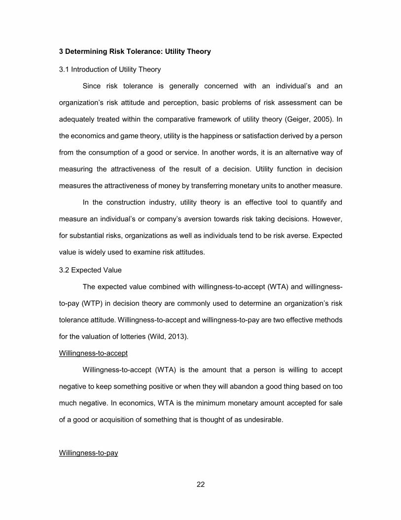
Risk Neutral
Different from risk aversion, if the decision maker is considered risk neutral, it
means that gain or loss of a specific dollar amount results in the same magnitude in
increasing or decreasing utility. In the aforementioned case, the utility of each hundred
dollars then shares the same increment.
Table 7 Sample Utility for Risk Neutrality
Monetary Value utility
$ - 0.00
$ 100.00 0.25
$ 200.00 0.50
$ 300.00 0.75
$ 400.00 1.00

30
Figure 4 Sample utility curve for risk neutrality
The utility curve for risk neutrality is usually shown as a straight line, which is same as the
risk indifference function.
Risk Seeking
Contrary to risk aversion, if an individual is considered risk seeking, it means that
gain of a specified amount of dollars increases the utility more than a loss of the same
amount of dollars decreases the utility.
0
0.1
0.2
0.3
0.4
0.5
0.6
0.7
0.8
0.9
1
0 50 100 150 200 250 300 350 400
uti
lity
dollars
Sample utility curve for risk neutrality

31
Table 8 Sample Utility for Risk Seeking
monetary value utility
$ - 0.00
$ 100.00 0.10
$ 200.00 0.25
$ 300.00 0.50
$ 400.00 0.90
Figure 5 Sample utility curve for risk seeking
As shown in Figure 5, if the individual is considered risk seeking, his utility curve is always
convex up.
3.3.2 Create Utility Function
As mentioned in the previous section, the utility curve can be plotted if the utilities
are pre-determined; however, sometimes the utility of a monetary value is difficult to
0
0.1
0.2
0.3
0.4
0.5
0.6
0.7
0.8
0.9
1
0 50 100 150 200 250 300 350 400
uti
lity
dollars
sample utility curve for risk seeking

32
determine because of its human dynamic. In order to mathematically map the physical
measure of monetary value and the perceived value of money, utility functions are
required to assess utility.
Lee Merkhofer (2003) suggested that the goal of a risk averse decision maker is
to maximize a certain equivalent. The researcher defined the term “certain equivalent” as
the amount of pay off that an agent would have to receive to be indifferent between that
pay off and a given gamble. The utility function is used to estimate the results from the
simple gamble, and the outputs can be used to infer certain equivalents of more
complicated risks. For example, a decision maker is facing a risky project that ranges from
$0 to $1,000,000. It is difficult to determine the certain equivalent for this project directly;
however, a certain equivalent can be determined when the risky project is transformed to
a two-end gamble with an equal chance of yielding $0 or $1,000,000. Although the
expected return of the gamble is $500,000, the certain equivalent will be less than the
expected return if the decision maker is considered risk averse. Assume the outcome $0
has a utility of zero, probability of “p” and the outcome $1,000,000 has a utility of one,
probability of (1-p). The certain equivalent holds that:
𝑢(𝑐𝑒𝑟𝑡𝑎𝑖𝑛 𝑒𝑞𝑢𝑖𝑣𝑎𝑙𝑒𝑛𝑡) = 𝑝 × u($0) + (1 − 𝑝)𝑢($1000,000)
In this case:
𝑢(𝑐𝑒𝑟𝑡𝑎𝑖𝑛 𝑒𝑞𝑢𝑖𝑣𝑎𝑙𝑒𝑛𝑡) = 0.5 × 0 + 0.5 × 1 = 0.5
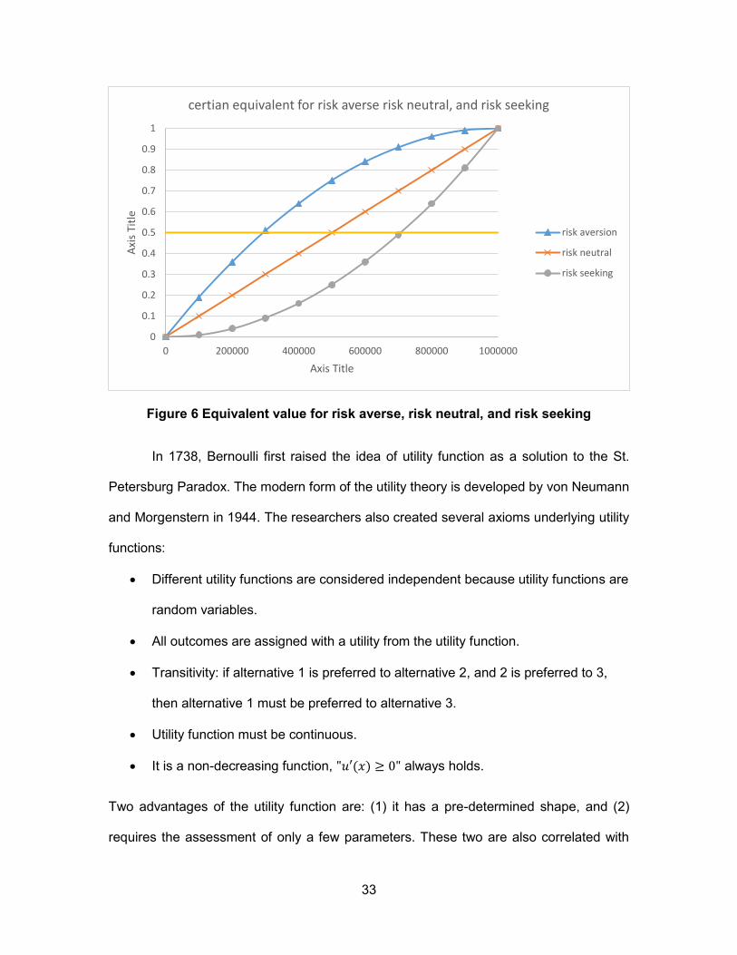
So, the certain equivalent is the monetary amount that has a utility of 0.5 generated from
the utility function. As shown in Figure 6, if the decision maker is risk averse, and the utility
function is concave down, the certain equivalent is less than the expected return. If the
decision maker is risk neutral, the utility function is a straight line, and the certain
equivalent is equal to the expected return. If the decision maker is risk seeking, the utility
function is convex up, and the certain equivalent is greater than the expected value.
33
Figure 6 Equivalent value for risk averse, risk neutral, and risk seeking
In 1738, Bernoulli first raised the idea of utility function as a solution to the St.
Petersburg Paradox. The modern form of the utility theory is developed by von Neumann
and Morgenstern in 1944. The researchers also created several axioms underlying utility
functions:
Different utility functions are considered independent because utility functions are
random variables.
All outcomes are assigned with a utility from the utility function.
Transitivity: if alternative 1 is preferred to alternative 2, and 2 is preferred to 3,
then alternative 1 must be preferred to alternative 3.
Utility function must be continuous.
It is a non-decreasing function, "𝑢′(𝑥) ≥ 0" always holds.
Two advantages of the utility function are: (1) it has a pre-determined shape, and (2)
requires the assessment of only a few parameters. These two are also correlated with
0
0.1
0.2
0.3
0.4
0.5
0.6
0.7
0.8
0.9
1
0 200000 400000 600000 800000 1000000
Axi
s Ti
tle
Axis Title
certian equivalent for risk averse risk neutral, and risk seeking
risk aversion
risk neutral
risk seeking

34
each other as the parameters will determine the shape of the utility function, and the shape
of the utility function determines the degree of aversion of taking risks. For example, Figure
7 shows two concave utility functions: utility function 1 and utility function 2, and both of
them are considered as risk averse.
Figure 7 Sample utility function for risk aversion
In general, both utility functions in Figure 7 are considered as risk averse; however,
if comparing the two utility functions to each other, utility function 1 is relatively risk seeking
and utility function 2 is relatively risk averse. The reason is that utility function 2 converges
faster than utility function 1, so the same amount of monetary value will bring an
organization that holds utility function 2 a higher satisfaction level, which is a higher utility
value. As a result, for the risk averse utility function, the more the plot bends over, the
more risk aversion is represented. In parallel with the risk averse utility function, Figure 8
shows two utility functions for risk seeking: utility function 3 and utility function 4.
-0.8
-0.6
-0.4
-0.2
0
0.2
0.4
0.6
0.8
1
1.2
-1 0 1 2 3 4
uti
lity
millions
Sample utility function for risk aversion
utility function 1
utility function 2

35
Figure 8 Sample utility function for risk seeking
Utility function 3 and utility function 4 are considered risk seeking, since the shape of both
curves are convex up. However, utility function 3 is considered to be relatively risk averse
when compared to the other, because the same monetary amount increment brings more
utility to utility function 4.
3.3.3 Common Types of Utility Functions
From previous research, the most commonly used utility function are:
1. Exponential utility function:
𝑢(𝑥) = 1 − 𝑒−𝛼𝑥, 𝛼 > 0
2. Logarithmic utility function:
𝑢(𝑥) = 𝑙𝑜𝑔 (𝑥)
3. Power utility function:
𝑢(𝑥) = 𝑥𝛼
4. Iso-elastic utility function:
-1.5
-1
-0.5
0
0.5
1
1.5
2
-1 -0.5 0 0.5 1 1.5 2 2.5 3 3.5
uti
lity
millions
Sample utility function for risk seeking
utility function 3
utility function 4
36
𝑢(𝑥) =𝑥1−𝜂
1 − 𝜂, 𝜂 < 1
Although these four utility functions are widely used, this research tends to focus on
exponential utility function to model construction organizations’ risk tolerance.
3.3.3.1 Exponential Utility Function
Any decision facing the organization can be analyzed best if the organization’s
attitude towards project risk is well known and represented in the analysis by an
appropriate utility function (Hulett, 2013). As mentioned in the previous section,
construction organizations often perceive a greater aversion to losses from failure of the
project than they benefit from a similar-size gain from project success. For example, in the
construction industry, the fear of losing $1 million usually overweighs the benefit of gaining
$1 million. Exponential utility function is a common choice for representing a construction
organization’s risk averse attitude, because of its convenience when risk are presented. It
also has an appropriate curvature for risk aversion since the normal exponential utility
function is always concave.
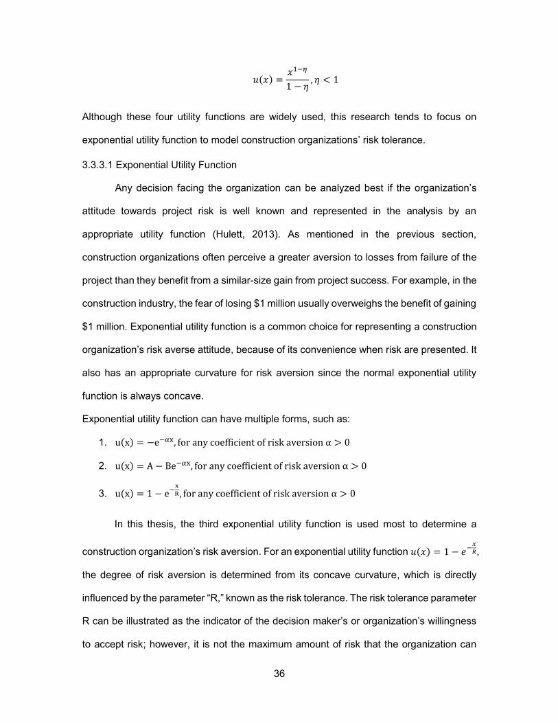
Exponential utility function can have multiple forms, such as:
1. u(x) = −e−αx, for any coefficient of risk aversion α > 0
2. u(x) = A − Be−αx, for any coefficient of risk aversion α > 0
3. u(x) = 1 − e−x
R, for any coefficient of risk aversion α > 0
In this thesis, the third exponential utility function is used most to determine a
construction organization’s risk aversion. For an exponential utility function 𝑢(𝑥) = 1 − 𝑒−𝑥
𝑅,
the degree of risk aversion is determined from its concave curvature, which is directly
influenced by the parameter “R,” known as the risk tolerance. The risk tolerance parameter
R can be illustrated as the indicator of the decision maker’s or organization’s willingness
to accept risk; however, it is not the maximum amount of risk that the organization can

37
afford to lose. It is difficult to discover the organization’s risk tolerance parameter by
directly asking people about their degree of risk aversion or the risk tolerance parameter,
but there are still several ways to determine the risk parameter for an organization. The
most widely used method to determine the risk tolerance parameter R is to ask senior
decision makers, ideally the CEO, to answer the following hypothetical question (Lee
Merkhofer, 2003):
Suppose you have an opportunity to make a risky, but potentially
profitable investment. The required investment is an amount R that, for
the moment, is unspecified. The investment has a 50-50 chance of
success. If it succeeds, it will generate the full amount invested, including
the cost of capital, plus that amount again. In other words, the return will
be R if the investment is successful. If the investment fails, half the
investment will be lost, so the return is minus R/2. So, what is the
maximum amount (R) you would accept in this investment?
Figure 9 What is the maximum amount (R) you would accept (Lee Merkhofer
Consulting, 2011)
As shown in Figure 9, the expected profit return of this investment is determined
to be R/4, the maximum return is 2R, and the minimum return is R/2. The risk tolerance R
is the monetary amount that a decision maker or an organization is indifferent between
investing and not investing. In the construction industry, if the amount R is low, most
Return
0.5
R
-R/20.5 x R + 0.5 x (-R/2) = 0.25 R
Expected Value
Success
Failure
0.5

38
organizations would make the investment because most of them can bear the risk.
However, if R is very large, those organizations would not make the investment because
they cannot afford to lose. As a result, organizations with relatively larger risk tolerance R
are considered to be less risk averse. Lee Merkhofer Consulting suggests that the typical
risk tolerance at the CEO or Board level are often equal to about 20% of the organization’s
market value for publicly traded firms.
However, sometimes this method, when used to determine risk tolerance
parameter, is still vague for a decision maker of an organization. The question will be
clearer if this investment question is transferred to a lottery question. A sample lottery
question is shown as follows: “Assume there is a lottery game with two alternatives: the
first alternative is to win $50,000, the second alternative is to lose half, which is $25,000.
Will you play this lottery game?” If the decision maker’s answer is positive, by increasing
the monetary value, there is a peak point that the decision maker will not play this lottery
game, where the peak point is described as the risk tolerance parameter R.

39
Once the risk tolerance parameter is set, the exponential utility function can be
plotted for further analysis. Figure 10 illustrates the difference between exponential utility
functions corresponding to the different risk tolerance parameter R.
Figure 10 Sample exponential utility function
As shown in Figure 9, the utility function of the risk tolerance parameter R is equal
to 1 million bends over the most that it holds the highest risk aversion among these three
utility functions. When the exponential utility function is determined, it can be used to
compute the certain equivalent. Assume R equals 2 million, and the risk is a 50% chance
of -$1.5 million and 3.5 million. The procedures to define its certain equivalent are listed
as follow:
1. From Figure 10, determine the utility of -$1.5 million and $3.5 million.
𝑢(−1.5 𝑚𝑖𝑙𝑙𝑖𝑜𝑛) = −1.117
𝑢(3.5 𝑚𝑖𝑙𝑙𝑖𝑜𝑛) = 0.826
2. Determine the expected utility for this risk, which is
-4
-3.5
-3
-2.5
-2
-1.5
-1
-0.5
0
0.5
1
-2 -1.5 -1 -0.5 0 0.5 1 1.5 2 2.5 3 3.5 4
uti
lity
millions
Exponential utility function u(x)=1-e^(-x/R)
R = 1 million
R = 2 million
R = 3 million
40
0.5 × 𝑢(−1.5 𝑚) + 0.5 × 𝑢(3.5 𝑚) = 0.5 × (−1.117) + 0.5 × 0.826 = −0.146
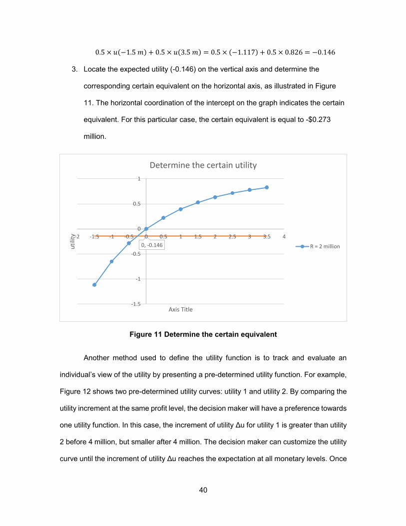
3. Locate the expected utility (-0.146) on the vertical axis and determine the
corresponding certain equivalent on the horizontal axis, as illustrated in Figure
11. The horizontal coordination of the intercept on the graph indicates the certain
equivalent. For this particular case, the certain equivalent is equal to -$0.273
million.
Figure 11 Determine the certain equivalent
Another method used to define the utility function is to track and evaluate an
individual’s view of the utility by presenting a pre-determined utility function. For example,
Figure 12 shows two pre-determined utility curves: utility 1 and utility 2. By comparing the
utility increment at the same profit level, the decision maker will have a preference towards
one utility function. In this case, the increment of utility Δu for utility 1 is greater than utility
2 before 4 million, but smaller after 4 million. The decision maker can customize the utility
curve until the increment of utility Δu reaches the expectation at all monetary levels. Once
0, -0.146
-1.5
-1
-0.5
0
0.5
1
-2 -1.5 -1 -0.5 0 0.5 1 1.5 2 2.5 3 3.5 4
uti
lity
Axis Title
Determine the certain utility
R = 2 million
Δu1
Δu2

41
the utility increment of a utility curve at each level is agreed upon by the decision maker
through the trial, this final utility curve expresses the decision maker’s attitude towards
profit. This method is more accurate than the utility function, but it requires more inputs
and time compared to the previous method.
Figure 12 Example of customized utility function
0
0.1
0.2
0.3
0.4
0.5
0.6
0.7
0.8
0.9
1
0 2 4 6 8 10
uti
lity
Profit (million)
utility 1
utility 2

42
4 Application of Utility Theory
4.1 Determine the Utility Curve for a Cumulative Project Cost
A cumulative distribution of project cost can be generated from the simulation tool
that reflects all the possible outcomes from the risks. Since a construction project usually
involves multiple risks, it is difficult to create a series of utility functions for each risk factor
encountered. Instead, the utility theory is applied to the cumulative distribution function
(CDF) as a whole. In order to fit CDF to the aforementioned exponential utility function,
the cumulative distribution of project cost is transferred into a distribution of potential profit.
The potential profit of a project can be defined through a pre-determined project
budget. This project budget is the critical value on the cumulative distribution of project
cost that also stands for the maximum risk capacity an organization can afford to lose.
4.1.1 Risk Capacity
Risk capacity (contractor) or budget (owner) is defined as how much risk the
individual or organization can afford. In detail, the Financial Service Authority Guidance
(2011) defines the capacity for loss as:
[The] customer’s ability to absorb falls in the value of their investment. If
any loss of capital would have a materially detrimental effect on their
standard of living, this should be taken into account in assessing the risk
that they are able to take.
In the construction industry, risk tolerance and risk capacity are always indispensable
topics to discuss in the project planning process. Although organizations with different risk
attitudes will lead to different risk tolerances, the risk capacities will not be influenced by
the risk attitudes. Malkiel (1996) proposed that risk tolerance is subjective, but individual’s
risk capacity can be measured by their position in the life cycle. A project’s state can be
reflected by comparing an organization’s risk tolerance and capacity. A large risk tolerance

43
with low capacity is a dangerous condition for a project, while a low tolerance with large
capacity means a missed opportunity. However, in contrast, risk capacity can affect the
risk tolerance. If a company has a large risk capacity, it may be more risk seeking in
investment since it can bear more loss, while a company with low risk capacity may be
more risk averse since it cannot afford to fail.
For a construction organization, especially for contractors, risk capacity is
understood as the amount of risk that the company is able to support in pursuit of its
objectives (COSO, 2012). In other words, the maximum risk capacity can be determined
as the bottom line of a project cost, where any cost exceeding the maximum risk capacity
will result in a negative net return in the end. There are multiple ways to determine the
maximum risk capacity for a project. Three major facts need to be considered.
Initial wealth – The more an organization has, the more it can afford to lose.
Existing risk profile – If a construction organization undergoes multiple projects,
its risk capacity may be relatively small compared to a same level organization
that only has one project at a time.
Project conditions – Risk capacity of a construction company varies between
different projects. A project with diverse risk factors will result in a higher risk
capacity, while a relatively safer project will decrease a company’s risk capacity,
since the possibility of the occurrence of unexpected consequence is small.
Similar to the previous section about the risk tolerance parameter R for expected utility,
the maximum risk capacity can be determined from a questionnaire and what if analysis.
However, most organizations determine their risk capacity from the company’s situation,
past history, and the market situation.

44
4.1.2 Create Utility Curve
Once the maximum risk capacity is determined, the potential profit can be calculated from
the original cumulative project cost as follows:
𝑝𝑜𝑡𝑒𝑛𝑡𝑖𝑎𝑙 𝑝𝑟𝑜𝑓𝑖𝑡 = 𝑚𝑎𝑥𝑖𝑚𝑢𝑚 𝑟𝑖𝑠𝑘 𝑐𝑎𝑝𝑎𝑐𝑖𝑡𝑦 − 𝑜𝑟𝑖𝑔𝑖𝑛𝑎𝑙 𝑝𝑟𝑜𝑗𝑒𝑐𝑡 𝑐𝑜𝑠𝑡
For example, assume a project suffers from various risk events. The simulated result gives
a project cost minimum $269,430.19 to maximum $324,739.12. Figure 13 is the plot of the
project cost as a cumulative distribution function.
Figure 13 CDF plot of project cost
Before processing further analysis, a probability distribution is fitted to the series
of the cost data collected. Vose (2010) indicates that a common problem in risk analysis
is fitting a probability distribution to a set of observation for a variable in order to be able
to make forecasts about the probability or frequency of occurrence in the future. Using
probability distribution is a scientific way of dealing with uncertainty and making informed
business decisions. In this case, normal distribution is selected as the fitting distribution of
0
0.2
0.4
0.6
0.8
1
1.2
260000.00 270000.00 280000.00 290000.00 300000.00 310000.00 320000.00 330000.00
pro
bab
ility
project cost
CDF plot of project cost

45
the CDF, as shown in Figure 14. For example, if the construction organization wants to
have 95% confidence that the project can be finished, the corresponding results from the
CDF are determined to be around $321,200.
Figure 14 CDF of project cost fitted by normal distribution
For this particular example, assume the maximum risk capacity is $310,000. The
potential profit is determined in the following Table 9. The resulting maximum potential
profit occurs when the project is finished within its minimum possible cost, which is
$40,569.81, while the worst situation is that the project loses $14,739.12 when the
simulation reaches the maximum project cost.
0
0.1
0.2
0.3
0.4
0.5
0.6
0.7
0.8
0.9
1
260000.00 270000.00 280000.00 290000.00 300000.00 310000.00 320000.00 330000.00
pro
bab
ility
project cost ($)
CDF of project cost fitted by normal distribution

46
Table 9 Project Cost and Potential Profit
Probability Project Cost Maximum Risk Capacity Potential Profit
0.0131025 269430.19 310000 40569.81
0.03684085 275251.83 310000 34748.17
0.06734714 279173.43 310000 30826.57
0.08515186 280842.80 310000 29157.20
0.12828786 284013.76 310000 25986.24
…… …… …… ……
0.94927746 321153.39 310000 -11153.39
0.95300505 321646.75 310000 -11646.75
0.95607325 322076.96 310000 -12076.96
0.95942121 322575.00 310000 -12575.00
0.97164611 324739.12 310000 -14739.12
As shown in Figure 15, the x axis is the probability generated from the normal
distribution, and the y axis is the potential profit with respect to the probability confidence.
The result shows that there is nearly 80% chance that this project can be finished within
the budget.

47
Figure 15 Probability confidence vs. potential profit
As the potential profit distribution is known, it can be applied to the utility function
determined in the previous section:
𝑢(𝑥) = 1 − 𝑒−𝑥𝑅
For this particular case, assume two opposite conditions:
1. The construction organization is risk averse and the risk tolerance parameter R is
equal to $10,000.
2. The construction organization is relatively risk seeking and the risk tolerance
parameter R is equal to $30,000.
Figure 16 shows the actual plot of the exponential utility function for the potential profit
with respect to the two different risk tolerance parameters.
-20000
-10000
0
10000
20000
30000
40000
50000
0 0.1 0.2 0.3 0.4 0.5 0.6 0.7 0.8 0.9 1
po
ten
tial
pro
fit
probability
Probability confidence that the project will finish within corresponding potential profit

48
Figure 16 Exponential utility function of potential profit
4.2 Determine the Utility for Project Risk
For a cumulative distribution function of project cost, a simple utility function cannot
be used to determine risk tolerance because the greatest utility will always be the
preference, which occurs at the minimum project cost in the series of data. However, as
the simulation result in Figure 13 shows, the probability to finish the project within the
minimum project cost $269,430.19 is nearly zero. In order to modify the exponential utility
function, another utility function of project risk is created.
The project risk utility function should also fulfill the requirement that the overall
risk attitude towards the project is risk aversion, and the utility is always proportional to the
project cost. Since the maximum project cost leads to the largest probability confidence to
finish the project within the estimated budget, the corresponding utility of the maximum
cost is determined to be 1, while on the opposite side, the minimum project cost should
have the lowest utility.
-4
-3.5
-3
-2.5
-2
-1.5
-1
-0.5
0
0.5
1
1.5
-20000 -10000 0 10000 20000 30000 40000 50000
uti
lity
potential profit ($)
Exponential utiltiy function of potential profit
R = 10000
R = 30000

49
4.2.1 Determine the Shape of the Risk Utility Function
As mentioned in the previous section, the risk utility function is always risk averse,
which means a higher uncertainty will reflect a larger drop in the overall utility. Assume a
project cost varies from $3 million to $4 million. The risk utility function should be plotted
in a concave curve as shown in Figure 17.
Figure 17 Sample risk utility function
The risk utility function should fulfill the requirement that 丨 Δu1丨 < 丨 Δu2丨 <
丨 Δu3丨, thus, logarithmic or exponential function is an appropriate choice for the utility
function. However, in order to estimate the risk utility more accurately, questionnaires can
be used for further analysis.
4.3 Two Utility Function Combination
As mentioned in the previous sections, one cumulative distribution curve of project
potential profit or project risk cannot be used to determine the risk tolerance because the
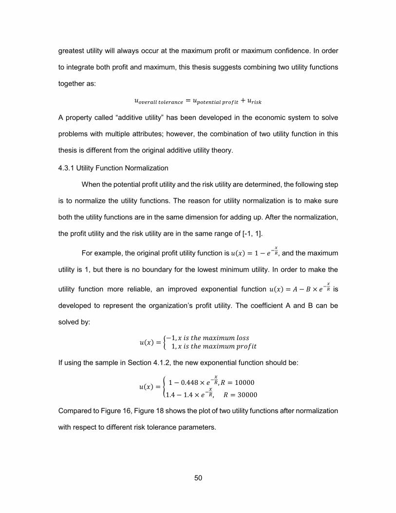
50
greatest utility will always occur at the maximum profit or maximum confidence. In order
to integrate both profit and maximum, this thesis suggests combining two utility functions
together as:
𝑢𝑜𝑣𝑒𝑟𝑎𝑙𝑙 𝑡𝑜𝑙𝑒𝑟𝑎𝑛𝑐𝑒 = 𝑢𝑝𝑜𝑡𝑒𝑛𝑡𝑖𝑎𝑙 𝑝𝑟𝑜𝑓𝑖𝑡 + 𝑢𝑟𝑖𝑠𝑘
A property called “additive utility” has been developed in the economic system to solve
problems with multiple attributes; however, the combination of two utility function in this
thesis is different from the original additive utility theory.
4.3.1 Utility Function Normalization
When the potential profit utility and the risk utility are determined, the following step
is to normalize the utility functions. The reason for utility normalization is to make sure
both the utility functions are in the same dimension for adding up. After the normalization,
the profit utility and the risk utility are in the same range of [-1, 1].
For example, the original profit utility function is 𝑢(𝑥) = 1 − 𝑒−𝑥
𝑅, and the maximum
utility is 1, but there is no boundary for the lowest minimum utility. In order to make the
utility function more reliable, an improved exponential function 𝑢(𝑥) = 𝐴 − 𝐵 × 𝑒−𝑥
𝑅 is
developed to represent the organization’s profit utility. The coefficient A and B can be
solved by:
𝑢(𝑥) = {−1, 𝑥 𝑖𝑠 𝑡ℎ𝑒 𝑚𝑎𝑥𝑖𝑚𝑢𝑚 𝑙𝑜𝑠𝑠
1, 𝑥 𝑖𝑠 𝑡ℎ𝑒 𝑚𝑎𝑥𝑖𝑚𝑢𝑚 𝑝𝑟𝑜𝑓𝑖𝑡
If using the sample in Section 4.1.2, the new exponential function should be:
𝑢(𝑥) = {1 − 0.448 × 𝑒−
𝑥𝑅, 𝑅 = 10000
1.4 − 1.4 × 𝑒−𝑥𝑅, 𝑅 = 30000
Compared to Figure 16, Figure 18 shows the plot of two utility functions after normalization
with respect to different risk tolerance parameters.

51
Figure 18 Normalized profit utility curve
After the normalized profit utility curve is generated, organizations can compare
their risk appetite with the determined curve. For the above example, the maximum profit
of the project is rounded to $40,000 and the maximum loss is $14,700. Assume there is
an investment with two alternatives, winning the same amount as the maximum profit, or
losing the same amount as the maximum loss. An organization can self-determine the
probability distribution of these two alternatives; thus, the organization will participate in
the investment with the determined probability distribution. Assume an organization is risk
averse with a risk tolerance parameter R equal to 30000, as shown in Figure 18, the
probability “P” of winning $40,000 should fulfill the following equation:
1 × 𝑃 + (−1) × (1 − 𝑃) = 𝑌 − 𝑖𝑛𝑡𝑒𝑟𝑐𝑒𝑝𝑡 ≈ 0.5
Thus, the probability “P” of winning is at least 0.75 in order to participate. If the organization
is relatively risk seeking and its risk tolerance parameter R is equal to 10000, the
probability “P” of winning is dropped from 0.75 to 0.5. Organizations can self-check the
-1.5
-1
-0.5
0
0.5
1
1.5
-20000 -10000 0 10000 20000 30000 40000 50000
uti
lity
potential profit ($)
Normalized profit utility curve
R = 10000
R = 30000

52
potential risk utility function using the above approach in order to determine the correct
risk aversion attitudes.
The project risk utility function can also be normalized to a range of [-1, 1] by adding
a coefficient to the utility equation. For the example in Section 4.1.2, assume the original
risk utility function uses logarithmic function to represent its risk aversion degree, the risk
utility function is determined as 𝑢(𝑥) = 1 + 𝐴 × 𝑙𝑛 (𝑥
𝑚𝑎𝑥𝑖𝑚𝑢𝑚 𝑝𝑟𝑜𝑗𝑒𝑐𝑡 𝑐𝑜𝑠𝑡), which fulfills the
requirement that utility equals 1 when the project cost is at its maximum. The coefficient
A can be generated from the point (minimum project cost, -1). In the end, the risk utility
function for the above example is determined as the following equation:
𝑢(𝑥) = 1 + 10.67 × 𝑙𝑛 (𝑥
325000)
4.3.2 Overall Utility Formation
The core approach to determine an organization’s risk tolerance is to sum both
profit utility and risk utility together to obtain an overall utility function indicating the risk
attitudes with respect to not only the profit, but also the potential risk from seeking profit.
The normalized utility function will ensure that the overall utility equals zero in both the
best and worst cases, because the maximum project cost has a utility of -1 for potential
profit and 1 for project risk, while the minimum project cost has the opposite situation.
In order to plot the overall utility function, the x-axis of the project potential utility function
should transfer from the profit to the project cost, which can be done by reflecting the curve
about the y-axis, as shown in Figure 19. Based on the sample project in section 4.1.2, the
project risk utility function is shown in Figure 20.

53
Figure 19 Profit utility function with respect to project cost
Figure 20 Project risk utility function with respect to project cost
-1.5
-1
-0.5
0
0.5
1
1.5
260000 270000 280000 290000 300000 310000 320000 330000uti
lity
project cost ($)
Profit utility function
R = 10000
R = 30000
-1.5
-1
-0.5
0
0.5
1
1.5
260000 270000 280000 290000 300000 310000 320000 330000uti
lity
project cost ($)
Project risk utility function

54
Once the potential profit utility function and the project risk utility function are in the
same dimension, the following step is to add two functions to create an overall utility curve
that represents the organization’s overall risk tolerance, as shown in Figures 21 and 22.
Figure 21 Overall utility function R=10000
-0.2
0
0.2
0.4
0.6
0.8
1
1.2
260000 270000 280000 290000 300000 310000 320000 330000
uti
lity
project cost ($)
Overall utility function R=10000

55
Figure 22 Overall utility function R=30000
As shown in the above figures, the optimal project cost for R equal to 10000 is
somewhere between $306,978.2 and $307,070.9, while the optimal project cost for R
equal to 30000 is between $300,067.4 and $302,664.7. Since the sample is a hypothetical
small project, the estimated project cost for different risk tolerance parameter R is
relatively close; however, the organization with a higher risk aversion has a larger project
cost.
4.3.3 Determine the Weight of Utility Function
Although the normalization process translates two utility functions into the same
range for analyzing, the profit utility function and risk utility function may also be weighed
for other purposes. The weighed utility function should have the following formula that
balances the potential profit and risk:
𝑢𝑜𝑣𝑒𝑟𝑎𝑙𝑙 = 𝜆 × 𝑢𝑝𝑟𝑜𝑓𝑖𝑡 + (1 − 𝜆) × 𝑢𝑟𝑖𝑠𝑘
Although the approach of adding utility function is based on a rule that construction
organizations are always risk averse towards any type of project, there is still bias between
0
0.1
0.2
0.3
0.4
0.5
0.6
260000 270000 280000 290000 300000 310000 320000 330000
uti
lity
project cost ($)
overall utility function R=30000

56
how much risk the organization is willing to bear and the resulting profit it is willing to
pursue. In a normal situation, assume a construction organization is totally unbiased
between profit and risk; the related weight coefficient 𝜆 should be 0.5. However, the
attitude towards gain and loss is always a human dynamic that varies in different
circumstances. For example, if the organization values profit more than the corresponding
risks, the 𝜆 under such circumstances may have a range between (0.5, 1), which provides
a heavier weight to the profit side. To illustrate this graphically, assuming the new
estimated 𝜆 for a relatively aggressive construction company with a risk tolerance
parameter of R equal to 30000 is 0.7, the new overall utility curve from the previous
example is plotted in Figure 23. The optimal project cost is between $298,965.74 and
$299,516.62, which is less than the original value.
Figure 23 Overall utility curve with applied weight coefficient
-0.6
-0.4
-0.2
0
0.2
0.4
0.6
0.8
260000 270000 280000 290000 300000 310000 320000 330000
uti
lity
project cost ($)
overall utility curve R=30000

57
4.3.3.1 Weight Assessment
There are multiple ways to determine the weight coefficient. Survey is an effective
method to assess individual’s preferences between risk and profit, but it is difficult to
quantitatively determine the ratio between these two factors.
A simple method to determine the weight of utility function is to compare
individual’s preferences by assigning a hypothetic rate to the risk and profit. If an
organization can directly specify the ratio of the weights as 𝜆𝑝𝑟𝑜𝑓𝑖𝑡 = 2𝜆𝑟𝑖𝑠𝑘, then 𝜆𝑝𝑟𝑜𝑓𝑖𝑡
equals to 2/3 and 𝜆𝑟𝑖𝑠𝑘 equals to 1/3.
Another method is to compare the uncertainty amount with a sure amount in order
to manage the ratio between risk and profit. For example, if a project suffers from an
uncertainty which may cause 20% chance of losing $10,000, the organization is asked to
determine the sure amount they are willing to pay to eliminate the potential risk. Assume
the following equation holds; the ratio between the risk utility and profit utility can be
calculated from the sure amount determined in the above hypothetic question:
𝑒𝑥𝑝𝑒𝑐𝑡𝑒𝑑 𝑟𝑖𝑠𝑘 𝑖𝑚𝑝𝑎𝑐𝑡
𝑠𝑢𝑟𝑒 𝑎𝑚𝑜𝑢𝑛𝑡 𝑑𝑒𝑡𝑒𝑟𝑚𝑖𝑛𝑒𝑑=
𝜆𝑝𝑟𝑜𝑓𝑖𝑡
𝜆𝑟𝑖𝑠𝑘
The expected risk impact is calculated as the total impact multiplied by the occurrence
possibility, which is $2,000 in the above sample. If an organization is willing to pay $1,500
to eliminate the risk, then the ratio "𝝀𝒑𝒓𝒐𝒇𝒊𝒕
𝝀𝒓𝒊𝒔𝒌" is determined to be 4/3. Since the organization
only accepts to disburse $1,500 from potential profit to manage a risk with expected impact
of $2,000, the organization is considered to be profit biased.

58
5 Development of Simulation Tool
This chapter is intended to introduce a revised user interface of a simulation
template developed in Simphony.NET. The template is based on Program Evaluation
Review Technology (PERT), which is designed to represent and analyze the tasks
involved in a given project. PERT was first developed by the US navy in the 1960’s to
measure and forecast progress in the Polaris submarine missile research. However,
nowadays, it is widely used in the construction industry to model the construction schedule
and the related risks. Several software tools such as Microsoft Project, Primavera 6, which
is commonly used in project management, are designed in a PERT base.
5.1 Framework of PERT
The early version of PERT used to model project complete duration consists of
three core steps:
1. Identify the specific activities.
2. Determine the proper sequence of the activities.
3. Construct a network diagram.
Nowadays, PERT also can be used to model the project cost with respect to the
project uncertainties. The following sections briefly describe the theory of how PERT
works in the project planning process.
5.1.1 WBS
The first step to model the project schedule using PERT is to determine all the
tasks that the project requires and the order in which they must be completed. A work
breakdown structure (WBS) is the most appropriate method used to determine all the
tasks of a project. PMI (2004) defines the WBS as “a deliverable-oriented hierarchical
decomposition of the work to be executed by the project team, to accomplish the project
objectives and create required deliverable.” According to the Project Management Body

59
of Knowledge (PMBOK®), WBS can be used to effectively decompose the project scope,
to improve estimating, to better control the project execution and to more accurately verify
project completion (PMBOK, 2013).
In construction engineering, a common WBS allows people to visually see the
overall work scope. A typical WBS is presented in the form of a tree structure. Generally,
a project can be classified into three hierarchical levels, which are project, work package,
and work task. Figure 24 shows a sample WBS diagram of a simple house construction.
The highest level is always the project level, which only consists of one element that
identifies the project. In this diagram, the project of house construction includes three work
packages, which are internal work, foundation work, and external work. Each work
package also includes several sub work packages, and the lowest level of the WBS is the
work tasks allocated under the sub work packages. For example, the internal work has
two sub work packages, electrical and plumbing, and the electrical work package consists
of three work tasks, rough-in electrical, install and terminate, and HVAC equipment.

60
Construction of a house
Internal Work Foundation Work External Work
Electrical
Rough-in electrical
Install and terminate
HAVC equipment
Plumbing
Rough-in plumbing
Set fixtures
Test and clean
Excavation
Pour concrete
Cure & strip forms
Steel Erection
Steel columns
Beams
Joist
Masonry Work
Lay masonry
Install roof drains
Install toilet
roofing
Building Finshing
Paint walls
Ceiling tile
Hang wallpaper
carpet
Figure 24 Sample WBS for house construction (Mark Swidersik, 2012)

61
5.1.2 Basic Theory of PERT
In order to model the project schedule using PERT, the sequence of each work
package and the duration of each work task must be identified in the beginning. A sample
project precedence shown in Table 10 illustrates the general requirements for creating a
PERT model.
Table 10 Sample Project Sequence and Duration
Work Task Predecessor
Estimated Duration
Expected Duration Optimistic Mode Pessimistic
A - 3 6 8 5.83
B - 5 9 14 9.17
C A 4 7 9 6.83
D A 2 7 10 6.67
E C 4 10 15 9.83
F B, C 3 5 7 5.00
G D 4 8 11 7.83
H F 2 3 7 3.50
The conventional PERT method incorporates uncertainties in duration using three
estimates: optimistic, most likely, and pessimistic.
Optimistic time is the minimum possible duration required to accomplish a work
task,
Mode time is the most likely duration which is the best estimate duration to
represent the work task, and
Pessimistic time is the maximum possible duration required to accomplish a work
task.

62
The expected duration “T” is calculated using the formula:
𝑇 =𝑜𝑝𝑡𝑖𝑚𝑖𝑠𝑡𝑖𝑐 𝑑𝑢𝑟𝑡𝑖𝑜𝑛 + 4 × 𝑚𝑜𝑑𝑒 𝑑𝑢𝑟𝑎𝑡𝑖𝑜𝑛 + 𝑝𝑒𝑠𝑠𝑖𝑚𝑖𝑠𝑡𝑖𝑐 𝑑𝑢𝑡𝑎𝑖𝑜𝑛
6
However, the conventional PERT method has its weakness. Each work task can only have
one duration, instead of random activity duration. Lu and AbouRizk (2000) indicated that
one promising solution to PERT’s defects is to perform a formal stochastic simulation such
as the Monte Carlo Simulation. In the simulation based network analysis, work task
durations are randomly selected from the distribution that the user specifies, and the
overall project duration will be displayed in a cumulative distribution curve. Moreover, the
stochastic simulation can also be applied to the estimation of project cost, which reflects
the impacts of the uncertainties. By allowing users to consider the schedule risk and cost
risk associated with a project, the simulation based network analysis results in a more
accurate and realistic estimation of project completion time and overall cost (Hong, 2012).
5.1.3 PERT Network Diagram
PERT network diagram is usually presented as a chart that graphically represents
all the tasks in a project. There are two types of network diagrams, activity on arrow (AOA)
and activity on node (AON). The simulation template created in Simphony.NET is based
on AON network. To create an AON diagram, it is recommended to start with a node
named “start” and to finish with a node named “finish.” These two nodes are considered
as two activities with no durations. For example, Figure 25 is an AON diagram based on
the information given in Table 10.

63
Start
A
B
C
D
E
F
G
H
Finish
Figure 25 Sample AON diagram
The direction of the arrows on the lines indicates the sequence of tasks. In this
diagram, for example, activity A, D, and G must be completed in sequence, or activity F
can only start when both activity B and C are completed, etc.
The duration schedule calculation for a conventional PERT model is
straightforward by following the critical path method scheduling rule. Figure 26 shows the
sample scheduling for the project in Table 10. “S” means the start time of the activity and
“F” means the finish time. In a PERT network diagram, the finish time is usually equal to
the start time plus the activity duration.
S: 0F: 0
S: 0, F: 5.83
S: 0F: 9.17
S: 5.83F: 12.66
S: 5.83F: 12.5
S: 12.66F: 22.49
S: 12.66F: 17.66
S: 12.5F: 20.33
S: 17.66F: 21.16
S: 22.49F: 22.49
A
B
C
D
E
F H
G
Start Finish
Figure 26 PERT scheduling

64
5.2 Original PERT Template in Simphony.NET
The original PERT template in Simphony was developed by Hong and AbouRizk
in 2012. This section will briefly introduce the interface of the old template and identify the
limitations.
5.2.1 Structure of Original PERT Template
The original PERT template in Simphony consists of three core components, WBS,
RBS, and resource block.
WBS
The work breakdown structure is the main body of the template configuration shown in
Figure 27. Each node stands for one work task and they are connected in sequence using
the direction arrows as mentioned in the previous section.
Figure 27 Sample WBS for PERT template
There are multiple inputs for one work task, such as duration, fixed cost, variable cost,
and the resource allocation and risk assignment, which should be provided with the project
information.

65
Resource Block
Resource block is a collection table shown in Figure 28 that identifies all the
resources used in the project. Three categories: labour, equipment, and material, can be
inputted in the left side of the table, and the right side of the table identifies the operation
cost and the risk factors that influence the resource.
Figure 28 Resource block
RBS
The risk breakdown structure states the possible risk that influence project cost
and schedule and the resource operation. As shown in Figure 29, the RBS consists of the
risk category element, which is the intermediate level of RBS, and risk factor element.

66
Figure 29 Risk breakdown structure
The risk factor is defined at the lowest level of an RBS, which will be assigned into
work tasks and resource block. Each risk factor will require three inputs: (1) impact on cost,
(2) impact on delay, and (3) likelihood. During the risk assignment process, the user is
asked to determine the sensitivity of a risk factor that stands for the degree of the impact.
After the model is completed, the simulation process is developed, based on the
flowchart shown in Figure 30.

67
Create WBS and define WPs properties
Define resource information
No
Yes
i = i+1
Start
Resource-driven estimating?
Risk analysis?
Create RBS and define risk factors
Generate scheduling network
Assign resources to WPs
Assign risk factors to WPs and resouces
Specify number of iterations (N)
Create operation models inside of WPs
Set current iteration (i) = 1
and start simulation
Input data preprocessing
Simulate operation models
Simulated scheduling network
Generate reports and graphs
i = N?
A
A
Save simulation result
End
Yes
Yes
No
No
Figure 30 Flowchart of simulation process (Hong, 2012)
5.2.2 Limitations of Original Template
Several limitations of the original PERT template interface are found during
application. This section includes a discussion of current limitations.
1. During the application, it was found that the time required to build a simulation
model in the PERT template is much longer than other special purpose
templates.
2. The WBS appearance is still based on the CPM network instead of the PERT
network, and the project duration calculation is also based on the CPM method.
3. The template currently assumes an unlimited supply of resources. It can be
modified to consider resource-constrained scheduling.

68
4. For a construction company use, it is difficult to determine the risk breakdown
structure related with the impacts and corresponding sensitivity.
5. With an initialized RBS, a risk factor assigned to different work tasks will share
the same likelihood and impact.
6. The determined risk factors can only affect work packages; however, there are
risks that may influence the entire project (e.g., inaccurate estimation in the
planning).
7. The risk allocation process is complicated since both resources and work
packages need to be assigned by risk factors.
5.3 Revised PERT Template Interface
This section will introduce the new user interface of the revised PERT template.
Section 5.3.1 presents the modeling elements and their relationship. Section 5.3.2 gives
the information about input and output data processing.
5.3.1 Modeling Elements of PERT Template
The modeling elements of the revised PERT template are linked to each other, as
shown in Figure 31. The first element created in the template is the project element, whose
properties are the general information of the project. The project element requires two
inputs: (1) all the resources involved in the project including labour and equipment, and
(2) risk factors that will influence the entire project as a whole, such as inaccurate
estimation in planning, etc. The outputs of the element contain the report of the overall
simulation results, such as project schedule and cost.

69
Model
Scenario
Simphony.NET default structure; multiple scenarios are built for comparison or revision
Project element Resource profile (category/name/cost/quantity) Risk Factors (category/factor/likelihood/cost impact/
schedule impact)
Work Package element Risk Factors (category/factor/likelihood/cost impact/
schedule impact)
Work Task element Activity Duration Material Cost Resource Assignment (name/quantity) Risk Factors (category/factor/likelihood/cost impact/
schedule impact)
Figure 31 Template elements and relationship
The project element contains two child elements, work package element and work
task element, which structure the WBS of a project. The work package is an intermediary
element between project and work task, which integrates a series of work tasks into a
package.
There is only one necessary input for work package element, which is the risk
assignment. The risk factors assigned to a certain work package will influence all the work
tasks under it. The work task element is the main object to be analyzed in simulation-
based network scheduling. It includes properties such as duration, material associated
with the task, resources associated with the task, and the risk factors that will influence
the task. Figure 32 shows the network chart of the template.

70
Figure 32 Network diagram of the revised PERT template
Each work task can have resources and risk factors assigned in the schedule
network view. The resources assigned in the project element are directly applied to the
work task in order to perform resource-driven scheduling. The quantity of each resource
initialized in the project element will be considered as the resource constraint for
simulation.
The risk assignment is identical for project, work package, and work task element.
Risks applied to the project, work package, or work task have 5 properties: (1) risk
category, (2) risk factor name, (3) likelihood, (4) cost impact, and (5) schedule impact.
Each risk factor has an independent impact; therefore, a work task has a cumulative
impact when multiple risk factors materialize at the same time. Both cost impact and
schedule impact are entered, either deterministically (constant) or probabilistically
(distribution), as a percentage of the initial duration or cost. For example, if a work task
with a duration of 5 is influence by two risks (1) bad weather, and (2) bad geological
condition, assuming both risks have a likelihood of 1 and a schedule impact of 20%, the
new duration “D” for the task is calculated as:
𝐷 = 𝑜𝑟𝑖𝑔𝑖𝑛𝑎𝑙 𝑑𝑢𝑟𝑎𝑡𝑖𝑜𝑛 + 𝑜𝑟𝑖𝑔𝑖𝑛𝑎𝑙 𝑑𝑢𝑟𝑎𝑡𝑖𝑜𝑛 × (𝐵(1,1) × 20% + 𝐵(1,1) × 20%) = 7
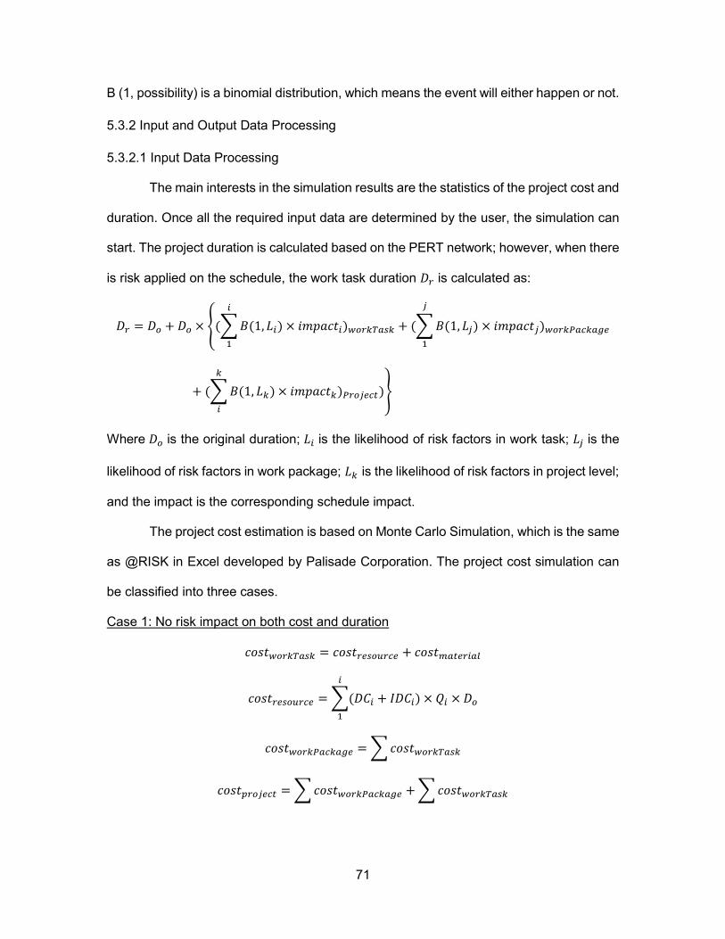
71
B (1, possibility) is a binomial distribution, which means the event will either happen or not.
5.3.2 Input and Output Data Processing
5.3.2.1 Input Data Processing
The main interests in the simulation results are the statistics of the project cost and
duration. Once all the required input data are determined by the user, the simulation can
start. The project duration is calculated based on the PERT network; however, when there
is risk applied on the schedule, the work task duration 𝐷𝑟 is calculated as:
𝐷𝑟 = 𝐷𝑜 + 𝐷𝑜 × {(∑ 𝐵(1, 𝐿𝑖
𝑖
1
) × 𝑖𝑚𝑝𝑎𝑐𝑡𝑖)𝑤𝑜𝑟𝑘𝑇𝑎𝑠𝑘 + (∑ 𝐵(1, 𝐿𝑗
𝑗
1
) × 𝑖𝑚𝑝𝑎𝑐𝑡𝑗)𝑤𝑜𝑟𝑘𝑃𝑎𝑐𝑘𝑎𝑔𝑒
+ (∑ 𝐵(1, 𝐿𝑘
𝑘
𝑖
) × 𝑖𝑚𝑝𝑎𝑐𝑡𝑘)𝑃𝑟𝑜𝑗𝑒𝑐𝑡)}
Where 𝐷𝑜 is the original duration; 𝐿𝑖 is the likelihood of risk factors in work task; 𝐿𝑗 is the
likelihood of risk factors in work package; 𝐿𝑘 is the likelihood of risk factors in project level;
and the impact is the corresponding schedule impact.
The project cost estimation is based on Monte Carlo Simulation, which is the same
as @RISK in Excel developed by Palisade Corporation. The project cost simulation can
be classified into three cases.
Case 1: No risk impact on both cost and duration
𝑐𝑜𝑠𝑡𝑤𝑜𝑟𝑘𝑇𝑎𝑠𝑘 = 𝑐𝑜𝑠𝑡𝑟𝑒𝑠𝑜𝑢𝑟𝑐𝑒 + 𝑐𝑜𝑠𝑡𝑚𝑎𝑡𝑒𝑟𝑖𝑎𝑙
𝑐𝑜𝑠𝑡𝑟𝑒𝑠𝑜𝑢𝑟𝑐𝑒 = ∑(𝐷𝐶𝑖 + 𝐼𝐷𝐶𝑖) × 𝑄𝑖 × 𝐷𝑜
𝑖
1
𝑐𝑜𝑠𝑡𝑤𝑜𝑟𝑘𝑃𝑎𝑐𝑘𝑎𝑔𝑒 = ∑ 𝑐𝑜𝑠𝑡𝑤𝑜𝑟𝑘𝑇𝑎𝑠𝑘
𝑐𝑜𝑠𝑡𝑝𝑟𝑜𝑗𝑒𝑐𝑡 = ∑ 𝑐𝑜𝑠𝑡𝑤𝑜𝑟𝑘𝑃𝑎𝑐𝑘𝑎𝑔𝑒 + ∑ 𝑐𝑜𝑠𝑡𝑤𝑜𝑟𝑘𝑇𝑎𝑠𝑘

72
Where 𝐷𝐶𝑖 is the direct cost of the resource; 𝐼𝐷𝐶𝑖 is the indirect cost of the resource; and
𝑄𝑖 is the quantity of the resource assigned into the work task.
Case 2: Risks’ impact on durations
𝑐𝑜𝑠𝑡𝑤𝑜𝑟𝑘𝑇𝑎𝑠𝑘 = 𝑐𝑜𝑠𝑡𝑟𝑒𝑠𝑜𝑢𝑟𝑐𝑒 + 𝑐𝑜𝑠𝑡𝑚𝑎𝑡𝑒𝑟𝑖𝑎𝑙
𝑐𝑜𝑠𝑡𝑟𝑒𝑠𝑜𝑢𝑟𝑐𝑒 = ∑(𝐷𝐶𝑖 + 𝐼𝐷𝐶𝑖) × 𝑄𝑖 × 𝐷𝑟
𝑖
1
𝑐𝑜𝑠𝑡𝑤𝑜𝑟𝑘𝑃𝑎𝑐𝑘𝑎𝑔e = ∑ costworkTask
costproject = ∑ costworkPackage + ∑ costworkTask
The calculation for project cost, which is influenced by schedule risk, is the same as the
original cost calculation; however, the only difference is application of the new duration Dr
into the resource cost calculation, since the duration change will only affect the operation
cost of the resource.
Case 3: Risk impact on cost
If there are risk factors influencing the project cost directly, the calculation follows
one rule: that the risks impact on duration is always applied before risks impact on cost.
costworkPackage = ∑ costworkTask
costproject = ∑ costworkPackage + ∑ costworkTask
costworkTask = costo + costr
costr = costo × {(∑ B(1, Li
i
1
) × impacti)workTask + (∑ B(1, Lj
j
1
) × impactj)workPackage
+ (∑ B(1, Lk
k
i
) × impactk)Project)}

73
Where costo is the original cost after risks impact on schedule; costr is the extra cost of a
work task caused by the risks impact on project cost; and the impact is the corresponding
cost impact.
5.3.2.2 Output Data Processing
The outputs for the project, work package, and work task contain three statistics,
the cost information, the start time, and the finish time. By implementing Monte Carlo
Simulation technique in this PERT template, the ranges of possible duration and cost are
calculated based on the impacts of associated factors. The statistics of outputs have
various properties including mean, standard deviation, minimum, maximum, kurtosis, and
skewness, etc.
The template’s overall results are displayed in the form of histograms and
cumulative distribution function graphs, as mentioned in the previous section. The
template can generate both duration CDF, and cost CDF for use in decision making.
Figure 33 shows a sample result of a cumulative distribution curve of project cost from the
simulation.

74
Figure 33 Sample cost result

75
6 Case Study
This chapter presents a hypothetical road construction case study in order to test
the new developed approach and to verify the simulation template. The case study was
used by Hong and AbouRizk (2011).
6.1 Project Information
The example used is a 1km long, one-way, two-lane road construction, which
encompasses 19 work packages, as shown in Table 11.
Table 11 WBS of the Hypothetical Road Construction (Hong, 2012)
Code Description ID
1 Country road construction 0
1.1 Mobilization 1
1.2 Preparation 2
1.2.1 Site clearing and grubbing 3
1.2.1.1 Sta. 130 to 750 4
1.2.1.2 Sta. 750 to 1,000 and Sta. 0 to 130 5
1.2.2 Earth cut (Sta. 400 to 750) and fill (Sta. 130 to 320) 6
1.2.3 Drainages 7
1.2.3.1 Storm Sewer manhole connected to curbs 8
1.2.3.2 Culvert installation 9
1.2.3.2.1 Culvert at Sta. 220 10
1.2.3.2.2 Culvert at Sta. 360 11
1.2.3.2.3 Culvert at Sta. 600 12

76
1.2.3.2.4 Culvert at Sta. 900 13
1.3 Road work 14
1.3.1 Base layers 15
1.3.1.1 250mm deep lime-stabilized layer 16
1.3.1.2 150mm deep crushed 20mm gravel layer 17
1.3.2 Asphalt paving layers 18
1.3.2.1 110mm deep first asphalt layer 19
1.3.2.2 60mm deep second asphalt layer 20
1.3.3 Curbs 21
1.3.3.1 Cast-in place concrete curbs 22
1.3.3.2 Saw-cut at 20 meter intervals 23
1.4 Finishing work 24
1.4.1 Painting stripes 25
1.4.2 Sign installation 26
1.4.3 Fine grading and seeding work 27
1.5 Demobilization 28
6.2 Create Simulation Model in PERT
The procedure of creating the road construction model in the PERT template can
be summarized as follows:
(1) Create a project element, which is the top level of the model that indicates the
project name and description, as shown in Figure 34.

77
Figure 34 Project element
Under the project element, create the WBS structure, which is indicated in Table
11. The activity duration and the relationship should also be identified at the same time.
Figure 35 displays the schedule network model created for the case study.

78
Figure 35 PERT network diagram

79
(2) Create the resource information under the project element. All the resources,
including labour and equipment and their related cost and quantity, should be
identified at this block. Figure 36 illustrates the user interface for the resource
definition.
Figure 36 Resource input table
(3) Assign the resources indicated in the last procedure into each work activity
according to the project information given. The quantity of resources also needs
to be identified in this step. Figure 37 shows a sample of resource allocation of
the activity “asphalt level 1”.

80
Figure 37 Assign resource into activities
(4) Input the material cost for each activity if available. The material cost is
determined as a lump sum price for each activity and pre-calculation is required.
From the project information provided, the material cost can be calculated using
the following equation:
material cost = unit cost ($/unit) × quantity
For example, the first asphalt layer is estimated to be 13,545 m2, and the unit
cost for asphalt is $35.55/m2, so the total material cost for this activity is
$481,524.8.
(5) Identify the risk factors that influence the project, work packages, and work
activities. Identify the risk impacts on both schedule and cost. A single work task
can be impacted by multiple risk events, which are considered as independent. A
risk factor consists of 5 components: (1) risk category, (2) risk factor, (3)
likelihood, (4) impact on schedule, and (5) impact on cost. In order to create a
simulation model to estimate the uncertainty of the project, the risk information
should be provided in advance. In this hypothetical case, two risk events, conflict
between parties and unfavourable market condition, are determined as the key

81
factors that influence the entire project. These two are directly assigned in the
project level, as shown in Figure 38.
Figure 38 Risk assignment sample
Other risk factors such as weather condition, resource availability, and labour
skill, etc. are assigned into each work activity as indicated in the project
information.
(6) After assigning all the risk factors into the WBS, specify the desired number of iterations
for the Monte Carlo Simulation and the expected percentile for the result, then execute
the simulation.
6.3 PERT Template Output
After simulating the model 200 times, the possible range of project cost and
duration are generated. Figures 39 and 40 display the statistics of the estimated project
durations and costs, respectively, in a CDF diagram. The results show that the completion
time of this road construction project is in a range of [82.4, 105.4] days, and the mean
completion time is 94.7 days. The 85 percentile of project duration is estimated to be 100.1
days, which means there is 85 percent chance that this project will be finished in 100 days.
A possible range of the project completion cost is [2,506,257.417, 3,294,163.042] dollars

82
and 85 percentile of the project cost is determined by the CDF diagram provided which is
$3,055,374.417.
Figure 39 CDF graph of the project completion duration
Figure 40 CDF graph of the project completion cost

83
The PERT template also provided reports for analysis. Table 12 displays the cost
reports for each work activity, and the risk allowance explains the amount of money that
organization spends on the risk events. Table 13 displays the cost report of the resource
category.
Table 12 Project Cost of WBS
WBS Minimum Mean Maximum % Percentile
(0.85)
Risk
Allowance
Road
Construction
$ $ $ $ $
2506257.42 2894676.4 3294163 3048176.08 551826.27
asphalt level 1 $ $ $ $ $
585397.04 716639.35 966072.81 809654.4 131242.31
asphalt level 2
$ $ $ $ $
346631.14 427286 565870.3 479708.36 80654.86
Clearing 1
$ $ $ $ $
85033.8 103257.61 140543.43 114820.94 18223.81
Clearing 2
$ $ $ $ $
56689.2 68871.22 90972.27 76404.19 12182.02
Concrete Curbs
$ $ $ $ $
81936 82110.52 108365.03 84136.51 174.52
Culvert Sta 220
$ $ $ $ $
23737.12 29272.23 39100.25 32666.13 5535.11
Culvert Sta 360
$ $ $ $ $
23737.12 29119.65 39124.12 32339.05 5382.53
Culvert Sta 600 $ $ $ $ $

84
34625.68 42756.69 55537.48 47537.41 8131.01
Culvert Sta 900 $ $ $ $ $
34625.68 43014.76 54694.41 47713.35 8389.08
Curb Saw-Cut $ $ $ $ $
2190 2199.93 2731.48 2266.17 9.93
Demobilization $ $ $ $ $
14976 15751.75 20090.74 16754.45 775.75
Earth Work $ $ $ $ $
206799.36 308729.28 463332.95 368194.58 101929.92
Fine Grading $ $ $ $ $
103326.96 103736.44 136289.99 107240.45 409.48
Gravel Layer $ $ $ $ $
357565.04 440647.63 613820.15 504365.49 83082.59
Lime Layer $ $ $ $ $
289079.44 380813.77 518286.42 436892.68 91734.33
Mobilization $ $ $ $ $
11232 11897.15 15339.51 12614.17 665.15
paiting Strips $ $ $ $ $
21260 22514.84 27735 24352.26 1254.84
Sign installation $ $ $ $ $
15858 15899.97 18965.95 16256.58 41.97
Storm Sewer
Manhole
$ $ $ $ $
48150.56 50157.62 55167.95 52279.89 2007.06

85
Table 13 Resource Cost Report
Resource
Category
Resource
Name
Direct Cost Indirect Cost Total Cost
Minimum Mean Maximum Minimum Mean Maximum Minimum Mean Maximum
Labour Labourer 101304 105281.94 119559.09 55944 58140.8 66025.2 157248 163423 185584
Labour Cost Subtotal 101304 105281.94 119559.09 55944 58140.8 66025.2 157248 163423 185584
Equipment Crane 33150.6 34452.34 39124.37 10710 11130.6 12640 43860.6 45582.9 51764.3
Equipment Dozer 121942.8 153239.09 212834.82 20779.92 26113 36268.6 142723 179352 249103
Equipment Grader 75335.52 94258.22 128017.64 18177.12 22742.8 30888.4 93512.6 117001 158906
Equipment Loader 134250.48 139522.14 158442.56 26331.48 27365.5 31076.4 160582 166888 189519
Equipment Paver 42076.8 53769.34 74877.85 6664.32 8516.24 11859.5 48741.1 62285.6 86737.4
Equipment Pneumatic
Roller 12254.4 15659.72 21807.34 3637.44 4648.23 6473.01 15891.8 20308 28280.4
Equipment Tandem
Roller 20836.8 26627.05 37080.17 7081.92 9049.88 12602.6 27918.7 35676.9 49682.8
Equipment Truck 25254 25329.4 30837.17 7596 7618.68 9275.33 32850 32948.1 40112.5
Equipment Vibration
Roller 266666.4 333647.4 453146.2 63903.84 79955.1 108592 330570 413603 561738

86
Equipment Cost Subtotal 731767.8 876504.7 1156168.13 164882.04 197140 259676 896650 1073645 1415844
Total 833071.8 981786.65 1275727.21 220826.04 255281 325701 1053898 1237067 1601428

87
6.3 Determine Organization’s Risk Appetite
This section illustrates how the newly developed risk tolerance assessment
approach works in this hypothetical case. Assume that after the model simulates 200 times,
the overall CDF curve is shown in Figure 41. From the previous experience, we know that
most likely, this curve can be converted into a normal distribution curve as shown in Figure
42.
Figure 41 CDF curve of project cost
0
0.2
0.4
0.6
0.8
1
1.2
2400000 2600000 2800000 3000000 3200000 3400000
pro
bab
ility
project cost ($)
CDF curve of project cost

88
Figure 42 CDF curve of project cost converted to normal distribution curve
As mentioned in Chapter 4, the following step is to determine a cost capacity for
the organization based on their company situation, market situation and other important
factors. The capacity determined on the CDF curve will potentially illustrate the possible
gain and loss in this road construction project. In this case, assume the risk capacity for
an organization is determined to be $3,000,000 for this road construction project, then the
potential gain and loss graph is illustrated in Figure 43.
Figure 43 Potential gain and loss of the project
0
0.2
0.4
0.6
0.8
1
1.2
2400000 2600000 2800000 3000000 3200000 3400000
pro
bab
ility
project cost ($)
0
0.2
0.4
0.6
0.8
1
1.2
-400000 -200000 0 200000 400000 600000
pro
bab
ility
potential gain and loss

89
The y axis of the above diagram shows that the probability of making profit. For
example, there is approximately only 10% chance that the organization can complete the
project with at least $300,000 gain, or there is approximate 40% chance that the
organization can complete the project with at least $150,000 gain. On the negative side,
the organization can complete the project with 90% confidence that the worst situation of
the outcome is only losing $100,000.
The following step is to apply the utility function to the potential profit curve. The
risk tolerance parameter R in this case study is pre-determined to be $250,000, and the
utility curve obtained using the following exponential utility function u(x) = 1 − e−x
R, where
R is 250000, is shown in Figure 44. Figure 45 shows the normalized utility curve for the
potential profit where the new utility function is determined as u(x) = 1.083 − 0.643 ∗ e−x
R.
Figure 44 Utility function of potential profit
-2.5
-2
-1.5
-1
-0.5
0
0.5
1
1.5
-400000 -200000 0 200000 400000 600000
uti
lity
potential gain and loss ($)
Y-Values
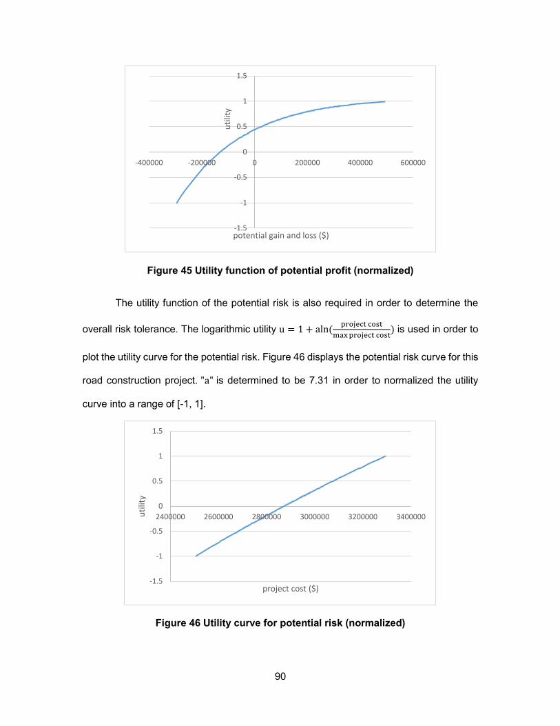
90
Figure 45 Utility function of potential profit (normalized)
The utility function of the potential risk is also required in order to determine the
overall risk tolerance. The logarithmic utility u = 1 + aln (project cost
max project cost) is used in order to
plot the utility curve for the potential risk. Figure 46 displays the potential risk curve for this
road construction project. "a" is determined to be 7.31 in order to normalized the utility
curve into a range of [-1, 1].
Figure 46 Utility curve for potential risk (normalized)
-1.5
-1
-0.5
0
0.5
1
1.5
-400000 -200000 0 200000 400000 600000
uti
lity
potential gain and loss ($)
-1.5
-1
-0.5
0
0.5
1
1.5
2400000 2600000 2800000 3000000 3200000 3400000uti
lity
project cost ($)

91
The last step is to determine the weight of both utility functions. The simplest way
is to determine the ratio "𝛌𝐩𝐫𝐨𝐟𝐢𝐭
𝛌𝐫𝐢𝐬𝐤" as mentioned in Chapter 4. In this hypothetical case,
assume the decision maker is indifferent between seeking profit or safely completing the
project, thus the overall utility for this project is shown in Figure 47.
Figure 47 Overall utility function
At the lowest project cost, the organization has the opportunity to make the
greatest profit, but there is almost a 100% chance that construction cannot finish within
the budget; at the maximum project cost, the organization will have maximum confidence
to complete the project, but the overall net value will be negative. From the data analysis,
the highest utility occurs in the cost range [2988138.107, 2988200.85] dollars. So the most
reasonable project cost, which will reflect organization’s attitude towards risk, is around
$2,988,200. Compared to the original 85 percentile of the cumulative project cost
($3,055,375), the new project cost is slightly biased towards risk. However, the new cost
is still above the 80th percentile of the overall distribution, which means that the
organization is still considered risk averse.
-0.1
0
0.1
0.2
0.3
0.4
0.5
0.6
0.7
0.8
2400000 2600000 2800000 3000000 3200000 3400000
uti
lity
project cost ($)

92
7 Conclusion
This chapter summarizes the work conducted in the research. It also outlines the
gap of the current work and recommendations for future enhancement.
7.1 Conclusion
In the current construction industry, simulation is a significantly useful technology
that can assist engineer’s decision making on project planning and estimation, especially
towards uncertainties. Although simulation can provide a range of project cost or duration,
it is still short of an analytical method to determine how much risk the organization is willing
to take. The objective of this research was to develop an approach that can assist decision
making on what percentile to use from a cumulative distribution function of project cost to
reflect the organization’s risk appetite and overall acceptance of risk.
The main contributions of this research are:
1. It developed an approach based on utility theory that can model an organization’s
risk attitude towards profit and potential loss. Two utility functions were
developed. One reflects an organization’s appetite towards potential profit and
the other reflects its tolerance towards potential risk in a specific project. Both
utility functions are determined from the cumulative distribution curve of project
cost, which was generated from the simulation tool. By combining the
aforementioned two utility functions, a balanced utility curve is obtained that
illustrates the overall utility for the organization towards a specific project.
2. In order to enhance the quantitative risk tolerance analysis, a special purpose
template in Simphony.NET, based on program evaluation and review technology
(PERT), was re-developed. The template provides an integrated cost/schedule
model and transforms the model to simulation-based planning, in which
uncertainties of project cost and schedule are evaluated through Monte Carlo
Simulation.

93
7.2 Limitations and Future Recommendations
This research is intended to provide a prototype for organizations which raises
the topic of how much risk they are willing to take. Utility theory is a good start to
examine risk attitudes. However, risk tolerance is such a subjective topic that it keeps
changing with the environment. It is difficult to have an approach that can 100%
adequately model risk attitudes.
The limitations of this research are:
1. An organization’s risk attitude is much more complicated than a simple
exponential utility function. More factors needs to be considered.
2. Organizations usually have their own risk statements that indicate how much risk
they can bear. This research did not consider the risk appetite statement.
3. The re-developed simulation template is still on a 24-hour schedule, a calendar
can be added to the template.
4. It is difficult to validate this approach because each organization has its own
strategy for determining how much risk they can bear.
For future research on this topic, data are required in order to compare the
analytical solution with the real situation. Surveys and interviews are also required in order
to determine the key factors that may influence the organization’s risk attitude. With all the
information provided, the utility function of risk tolerance can be more complicated and
reliable.

94
References
AbouRizk, S. M., and Hajjar, D. (1998). “A Framework for Applying Simulation in
Construction.” Canadian Journal of Civil Engineering, 25(3), 604-617.
AbouRizk, S.M. (2009). “Risk Analysis for Construction Project: A proactical guide for
engineers and project managers.” Edmonton: NSERC Industrial Research Chair in
Construction Engineering and Management.
Bell, D.E. (1988). “One-Switch Utility Functions and A Measure of Risk.” Management
Science, 34(12): 1416-1424.
Bell, D.E. (1995). “Risk, Return, and Utility.” Management Science, 41(1): 23-30.
Frijins, B., Gilbert, A., Lehnert, T., & Tourani-Rad, A. (2013). “Uncertainty avoidance, risk
tolerance and corporate takeover decisions.” Journal of Banking & Finance, (37):
2457-2471.
Froot, K.A, Venter, G.G. & Major, J.A. “Capital and Value of Risk Transfer.” Harvard
Business School, Boston.
Grable, J. & Lytton, R.H. (1999). “Financial risk tolerance revisited: the development of a
risk assessment instrument.” Financial Services Review, (8): 163-181.
Gilliam, J., Chatterjee, S., & Grable, J. (2010). “Measuring the Perception of Financial Risk
Tolerance: A Tale of Two Measures.” Association for Financial Counseling and
Planning Education.
Griffin, D., Li, K., Yue, H., & Zhao, L. (2009.) “Cultural Value and Corporate Risk-Taking.”
Hong, J., and AbouRizk, S. M. (2011). “A special purpose simulation tool for stochastic
precedence network scheduling.” Proceedings – CSCE Construction Specialty
Conference, CN-112-1-8.
Hanna, S., & Chen, P. (1997). “Subjective and Objective Risk Tolerance: Implications for
Optimal Portfolios.” Association for Financial Counseling and Planning Education.

95
Hanna, S.D., Gutter, M.S., & Fan, J.X. (2001). “A Measure of Risk Tolerance Based on
Economic Theory.” Association for Financial Counseling and Planning Education.
Hanna, S.D., & Lindamood, S. (2004). “An Improved Measure of Risk Aversion.”
Association for Financial Counseling and Planning Education.
Hsee, C.K., & Weber, E.U. (1999). “Cross-national Difference in Risk Preference and Lay
Predictions.” Journal of Behavioral Decision Making, 12: 165-179.
Hulett, D.T. (2006). “Use Decision Trees to Make Important Project Decisions.” Use
Decision Trees to Make Important Project Decisions, PM Network, Project
Management Institute, Newtown Square.
ISO. (2009). “ISO Guide 73.” Switzerland:ISO.
Kaheman, D., Lovallo, D. (1993). “Timid choices and bold forecasts: a cognitive
perspective on risk taking”. Mangement Science, 39(1): 17-31.
Kwak, Y.H., & LaPlace, K.S. (2005). “Examining risk tolerance in project-driven
organization.” Technovation, (25): 691-695.
Kindinger, J.P. (2002). “The Case for Quantitative Project Risk Analysis.” Decision
Applications Division, Probabilistic Risk Analysis Group (D-11), Los Alamos National
Laboratory.
Mustafa, M.A., & Al-Bahar, J.F. (1991). “Project Risk Assessment using the Analytic
Hierachy Process.” IEEE Transaction on Engineering Management, 38-1.
Project Management Institute. (2000). “A Guide to the Project Management Body of
Knowledge.” Pennsylvania: Project Management Institute.
Palisade Corporation. (2010). Palisade.
Rittenberg, L., & Martens, F. (2002) “Understanding and Communicating Risk Appetite.”
Enterprise Risk Management, COSO.
Statmen, M. (2010). “The cultures of risk tolerance.” Tilburg University.

96
Tversky, A., & Wakker, P. (1995), “Risk Attitudes and Decision Weights.” Econometrica,
63(6): 1255-1280.
Watson, J., & McNaughton, M. (2007). “Gender Difference in Risk Aversion and Expected
Retirement Benefits.” Financial Analysts Journal, 63(4), 52-62.
Wild, A., D. (2013). “Unraveling Risk Appetite.” Dissertation, Erasmus Universiteit
Rotterdam.
Weber, E.U., Blais, A.R., & Betz, N.E. (2002). “A Domain-specific Risk-attitude Scale:
Measuring Risk Perceptions and Risk Behaviors.” Journal of Behavioral Decision
Making, (15): 263-290.
Wei, L., Yuan, Y.N., Dong, W.D., & Zhang, B. (2011), “Study on Financial Risk
Assessment of Substation Project Based on Monte Carlo Simulation.” IEEE.