Synopsis

Quantitative Methods

1. Introducing Statistics: Some Simple Uses and Misuses

Learning Objectives

This module gives an overview of statistics, introducing basic ideas and concepts at a general

level, before dealing with them in greater detail in later modules. The purpose is to provide a

gentle way into the subject for those without a statistical background, in response to the

cynical view that it is not possible for anyone to read a statistical text unless they have read it

before. For those with a statistical background the module will provide a broad framework

for studying the subject.

Sections

1.1 Introduction

1.2 Probability

1.3 Discrete Statistical Distributions

1.4 Continuous Statistical Distributions

1.5 Standard Distributions

1.6 Wrong Use of Statistics

1.7 How to Spot Statistical Errors

Learning Summary

The purpose of this introduction has been twofold. The first aim has been to present some

statistical concepts as a basis for more detailed study of the subject. All the concepts will be

further explored later. The second aim has been to encourage a healthy scepticism and

atmosphere of constructive criticism which are necessary when weighing statistical evidence.

The healthy scepticism can be brought to bear on applications of the concepts introduced

so far as much as elsewhere in statistics. Probability and distributions can both be subject to

misuse.

Logical errors are often made with probability. For example, suppose a questionnaire

about marketing methods is sent to a selection of companies. From the 200 replies, it

emerges that 48 of the respondents are not in the area of marketing. It also emerges that 30

are at junior levels within their companies. What is the probability that any particular

questionnaire was filled in by someone neither in marketing nor at a senior level? It is

tempting to suppose that:

This is almost certainly wrong because of double counting. Some of the 48 non-

marketers are also likely to be at a junior level. If 10 respondents were non-marketers and at a

junior level, then:

Only in the rare case where none of those at a junior level were outside the marketing

area would the first calculation have been correct.

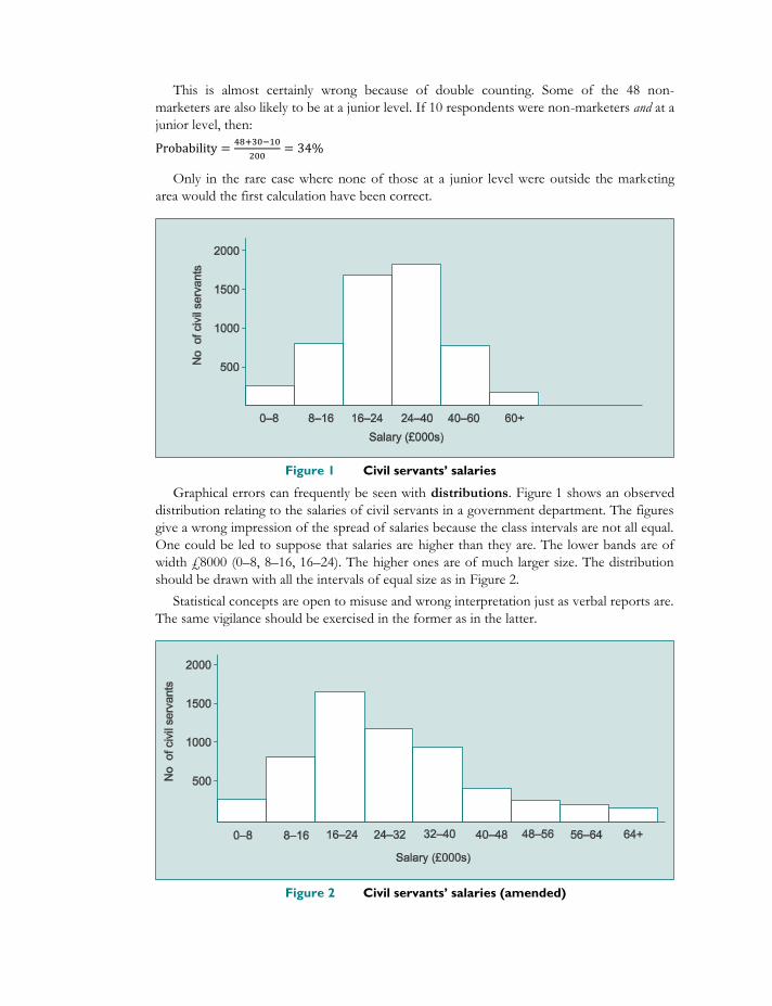
Figure 1 Civil servants’ salaries

Graphical errors can frequently be seen with distributions. ‎Figure 1 shows an observed

distribution relating to the salaries of civil servants in a government department. The figures

give a wrong impression of the spread of salaries because the class intervals are not all equal.

One could be led to suppose that salaries are higher than they are. The lower bands are of

width £8000 (0–8, 8–16, 16–24). The higher ones are of much larger size. The distribution

should be drawn with all the intervals of equal size as in ‎Figure 2.

Statistical concepts are open to misuse and wrong interpretation just as verbal reports are.

The same vigilance should be exercised in the former as in the latter.

Figure 2 Civil servants’ salaries (amended)

2. Basic Mathematics: School Mathematics Applied to

Management

Learning Objectives

This module describes some basic mathematics and associated notation. Some management

applications are described but the main purpose of the module is to lay the mathematical

foundations for later modules. It will be preferable to encounter the shock of the mathemat-

ics at this stage rather than later when it might detract from the management concepts under

consideration. For the mathematically literate the module will serve as a review; for those in

a rush it could be omitted altogether.

Sections

2.1 Introduction

2.2 Graphical Representation

2.3 Manipulation of Equations

2.4 Linear Functions

2.5 Simultaneous Equations

2.6 Exponential Functions

3. Data Communication

Learning Objectives

By the end of the module the reader should know how to improve data presentation. This is

important both in communicating data to others and in analysing data. The emphasis is on

the visual aspects of data presentation. Special reference is made to accounting data and

graphs.

Sections

3.1 Introduction

3.2 Rules for Data Presentation

3.3 The Special Case of Accounting Data

3.4 Communicating Data through Graphs

Learning Summary

The communication of data is an area that has been neglected, presumably because it is

technically simple and there is a tendency in quantitative areas (and perhaps elsewhere) to

believe that only the complex can be useful. Yet in modern organisations there can be few

things more in need of improvement than data communication.

Although the area is technically simple, it does involve immense difficulties. What exactly

is the readership for a set of data? What is the purpose of the data? How can the common

insistence on data specified to a level of accuracy that is not needed by the decision maker

and is not merited by the collection methods be overcome? How much accounting conven-

tion should be retained in communicating financial information to the layman? What should

be done about the aspects of data presentation that are a matter of taste? The guiding

principle among the problems is that the data should be communicated according to the

needs of the receiver rather than the producer. Furthermore, they should be communicated

so that the main features can be seen quickly. The seven rules of data presentation described

in this module seek to accomplish this.

(a) Rule 1: round to two effective digits.

(b) Rule 2: reorder the numbers.

(c) Rule 3: interchange rows and columns.

(d) Rule 4: use summary measures.

(e) Rule 5: minimise use of space and lines.

(f) Rule 6: clarify labelling.

(g) Rule 7: use a verbal summary.

Producers of data are accustomed to presenting them in their own style. As always there

will be resistance to changing an attitude and presenting data in a different way. The idea of

rounding especially is usually not accepted instantly. Surprisingly, however, while objections

are raised against rounding, graphs tend to be universally acclaimed even when not appropri-

ate. Yet the graphing of data is the grossest form of rounding. There is evidently a need for

clear and consistent thinking in regard to data communication.

This issue has been of increasing importance because of the growth in usage of all types

and sizes of computers and the development of large-scale management information

systems. The benefits of this technological revolution should be enormous but the potential

has yet to be realised. The quantities of data that circulate in many organisations are vast. It

is supposed that the data provide information which in turn leads to better decision making.

Sadly this is frequently not the case. The data circulate, not providing enlightenment, but

causing at best indifference and at worst tidal waves of confusion. Poor data communication

is a prime cause of this. It could be improved. Otherwise, one must question the wisdom of

the large expenditures many organisations make in providing untouched and bewildering

management data. One thing is clear. If information can be assimilated quickly, it will be

used; if not, it will be ignored.

4. Data Analysis

Learning Objectives

By the end of this module the reader should know how to analyse data systematically. The

methodology suggested is simple, relying very much on visual interpretation, but it is suitable

for most data analysis problems in management. It carries implications for the ways

information is produced and used.

Sections

4.1 Introduction

4.2 Management Problems in Data Analysis

4.3 Guidelines for Data Analysis

Learning Summary

Every manager sees the problem of handling numbers differently because each sees it mainly

in the (probably) narrow context with which he or she is familiar in his or her own work.

One manager sees numbers only in the financial area, another sees them only in production

management. The guidelines suggested here are intended to be generally applicable to the

analysis of business data in many different situations and with a range of different require-

ments. The key points are:

(a) Simple methods are preferable to complex ones.

(b) Visual inspection of well-arranged data can play a role in coming to understand them.

(c) Data analysis is like verbal analysis.

(d) The guidelines merely make explicit what comes naturally when dealing with words.

The need for better skills to turn data into real information in managerial situations is not

new. What has made the need so urgent in recent times is the exceedingly rapid development

of computers and associated management information systems. The ability to provide vast

amounts of data very quickly has grown enormously. It has far outstripped the ability of

management to make use of the data. The result has been that in many organisations

managers have been swamped with so-called information which in fact is no more than mere

numbers. The problem of general data analysis is no longer a small one that can be ignored.

When companies are spending large amounts of money on data provision, the question of

how to turn the data into information and use them in decision making is one that has to be

faced.

The inadequacy of the traditional subject of statistics to help in this area is now being

recognised. New skills and techniques are being developed. For example, Tukey has

developed an ‘alternative statistics’ called exploratory data analysis which is, in his view,

better able to deal with modern statistical problems. Time will reveal its value. Work such as

Tukey’s is an indication of the new circumstances that are unfolding within organisations

with regard to quantitative matters. The help with the problem given in this module is at a

much lower technical level than exploratory data analysis. The guidelines help non-statistical

managers make a start at understanding their own data in recognition of the fact that much

of the data analysis a typical manager has to do does not require a high level of technical

expertise.

5. Summary Measures

Learning Objectives

By the end of the module, the reader should know how large quantities of numbers can be

reduced to a few simple summary measures which are much easier to handle them than the

raw data. The most common measures are those of location and scatter. The special case of

summarising time series data with indices is also described.

Sections

5.1 Introduction

5.2 Usefulness of the Measures

5.3 Measures of Location

5.4 Measures of Scatter

5.5 Other Summary Measures

5.6 Dealing with Outliers

5.7 Indices

Learning Summary

In the process of analysing data, at some stage the analyst tries to form a model of the data

as suggested previously. ‘Pattern’ or ‘summary’ are close synonyms for ‘model’. The model

may be simple (all rows are approximately equal) or complex (the data are related via a

multiple regression model). Often specifying the model requires intuition and imagination.

At the very least, summary measures can provide a model based on specifying for the data

set:

(a) a measure of location;

(b) a measure of scatter;

(c) the shape of the distribution.

In the absence of other inspiration, these four attributes provide a useful model of a set

of numbers. If the data consist of two or more distinct sets (as, for example, a table), then

this basic model can be applied to each. This will give a means of comparison between the

rows or columns of the table or between one time period and another.

The first attribute (number of readings) is easily supplied. Measures of location and scat-

ter have already been discussed. The shape of the distribution can be found by drawing a

histogram and literally describing its shape (as with the symmetrical, U and reverse J

distributions seen earlier). A short verbal statement about the shape is often an important

factor in summarising or forming a model of a set of data.

Verbal statements have a more general role in summarising data. They should be short, no

more than one sentence, and only used when they can add to the summary. They are used in

two ways: first, they are used when the quantitative measures are inadequate; second, they

are used to point out important features in the data. For example, a table of a company’s

profits over several years might indicate that profits had doubled. Or a table of the last two

months’ car production figures might have a note stating that 1500 cars were lost because of

a strike.

It is important in using verbal summaries to distinguish between helpful statements

pointing out major features and unhelpful statements dealing with trivial exceptions and

details. A verbal summary should always contribute to the objective of adding to the ease

and speed with which the data can be handled.

6. Sampling Methods

Learning Objectives

By the end of this module the reader should know the main principles underlying sampling

methods. Most managers have to deal with sampling in some way. It may be directly in

commissioning a sampling survey, or it may be indirectly in making use of information based

on sampling. For both purposes it is necessary to know something of the techniques and,

more importantly, the factors critical to their success.

Sections

6.1 Introduction

6.2 Applications of Sampling

6.3 The Ideas behind Sampling

6.4 Random Sampling Methods

6.5 Judgement Sampling

6.6 The Accuracy of Samples

6.7 Typical Difficulties in Sampling

6.8 What Sample Size?

Learning Summary

It is most surprising that information collection should be so often done in apparent

ignorance of the concept of sampling. Needing information about invoices, one large

company investigated every single invoice issued and received over a three-month period, a

monumental task. A simple sampling exercise would have reduced the cost to around one

per cent of the actual cost with little or no loss of accuracy.

Even after it is decided to use sampling there is still, obviously, a need for careful plan-

ning. This should include a precise timetable of what and how things are to be done. The

crucial questions are: ‘What are the exact objectives of the study?’ and ‘Can the information

be provided from any other source?’ Without this careful planning it is possible to collect a

sample and then find the required measurements cannot be made. For example, having

obtained a sample of 2000 of the workforce, it may be found that absence records do not

exist, or it may be found that another group in the company carried out a similar survey 18

months before and their information merely needs updating.

The range of uses of sampling is extremely wide. Whenever information has to be col-

lected, sampling can prove valuable. The following list gives a guide to the applications that

are frequently encountered:

(a) market research of consumer attitudes and preferences;

(b) medical investigations;

(c) agriculture (crop studies);

(d) accounting;

(e) quality control (inspection of manufactured output);

(f) information systems.

In all applications, sampling is a trade-off between accuracy and expense. By sampling at

all one is losing accuracy but saving money. The smaller the sample the greater the accuracy

loss but the greater the saving. The trade-off has to be made in consideration of the accuracy

required by the objectives of the study and the budget available. Even when the full

population is investigated, however, the results will not be entirely accurate. The same

problems that occur in sampling – non-response, the sampling frame and bias – will occur

with the full population. The larger the sample size, the closer the accuracy will be to the

maximum accuracy that is obtainable with the full population. It may even be the case that

measurement errors may overwhelm sampling errors. For instance, even a slightly ambigu-

ous set of questions in an opinion poll can distort the results far more than any inaccuracy

resulting from taking a sample rather than considering the full population. The concern that

many managers have that sample information must be vastly inferior to population infor-

mation is ill-founded. A modest sample can provide results which are of only slightly lower

accuracy than those provided by the whole population and at a fraction of the cost.

7. Distributions

Learning Objectives

By the end of the module the reader should be aware of how and why distributions,

especially standard distributions, can be useful. Having numbers in the form of a distribution

helps both in describing and analysing. Distributions can be formed from collected data, or

they can be derived mathematically from knowledge of the situation in which the data are

generated. The latter are called standard distributions. Two standard distributions, the

binomial and the normal, are the main topics of the module.

Proof of some of the formulae requires a high level of mathematics. Where possible

mathematical derivations are given but since the purpose of this course is to explore the

practical applications of techniques, not their historical and mathematical development, there

are situations where the mathematics is left in its ‘black box’.

Note on Technical Sections: Section 7.3 ‘Probability Concepts’, Section 7.5.3 ‘Deriving

the Binomial Distribution’ and Section 7.6.3 ‘Deriving the Normal Distribution’ are technical

and may be omitted on a first reading.

Sections

7.1 Introduction

7.2 Observed Distributions

7.3 Probability Concepts

7.4 Standard Distributions

7.5 Binomial Distribution

7.6 The Normal Distribution

Learning Summary

The analysis of management problems often involves probabilities. For example, postal

services define their quality of service as the probability that a letter will reach its destination

the next day; electricity utilities set their capacity at a level such that there is no more than

some small probability that it will be exceeded and power cuts necessitated; marketing

managers in contracting companies may try to predict future business by attaching probabili-

ties to new contracts being sought. In such situations and many others, including those

introduced earlier, the analysis is frequently based on the use of observed or standard

distributions.

An observed distribution usually entails the collection of large amounts of data from

which to form histograms and estimate probabilities.

A standard distribution is mathematically derived from a theoretical situation. If an actual

situation matches (to a reasonable approximation) the theoretical then the standard distribu-

tion can be used both to describe and analyse the situation. As a result fewer data need be

collected.

This module has been concerned with two standard distributions: the binomial and the

normal. For both, the following have been described:

(a) the situations in which it can be used;

(b) its derivation;

(c) the use of probability tables;

(d) its parameters;

(e) how to decide whether an actual situation matches the theoretical situation on which the

distribution is based.

The mathematics of the distributions have been indicated but not pursued rigorously.

The underlying formulae, particularly the normal probability formula, require a relatively

high level of mathematical and statistical knowledge. Fortunately such detail is not necessary

for the effective use of the distributions because tables are available. Furthermore, the role

of the manager will rarely be that of a practitioner of statistics, rather he or she will have to

supervise the use of statistical methods in an organisation. It is therefore the central concepts

of the distributions, not the mathematical detail, that are of concern. To look at them more

deeply goes beyond what a manager will find helpful and enters the domain of the statistical

practitioner.

The distributions that have been the subject of this module are just two of the many that

are available. However, they are two of the most important and useful. The principles behind

the use of any standard distribution are the same, but each is associated with a different

situation. A later module will look at other standard distributions and their applications.

8. Statistical Inference

Learning Objectives

Statistical inference is the set of methods by which data from samples can be turned into

more general information about populations. By the end of the module, the reader should

understand the basic underlying concepts. Statistical inference has two main parts. Estima-

tion is concerned with making predictions and specifying their accuracy; significance testing

is concerned with distinguishing between a result arising by chance and one arising from

other factors. The module describes some of the many different types of significance test. As

in the last module, some of the mathematics will have to be left in a ‘black box’.

Sections

8.1 Introduction

8.2 Applications of Statistical Inference

8.3 Confidence Levels

8.4 Sampling Distribution of the Mean

8.5 Estimation

8.6 Basic Significance Tests

8.7 More Significance Tests

8.8 Reservations about the Use of Significance Tests

Learning Summary

Statistical inference belongs to the realms of traditional statistical theory. Its relevance lies in

its applicability to specialised management tasks, such as quality control and market research.

Most managers would find that it can only occasionally be applied directly to general

management problems. Its major value is that it encompasses ideas and concepts which

enable problems to be viewed in broader and more structured ways.

Two areas have been discussed, estimation and significance testing. New theory – confi-

dence levels, the sampling distribution of the mean, the central limit theorem and the

variance sum theorem – has been introduced.

The conceptual contribution that estimation makes is to concentrate attention on the

range of a business forecast rather than merely the point estimate. To take a previous market

research example, the estimate that 61 per cent of male toiletries are purchased by females

sounds fine. But what is the accuracy of the estimate? The 61 per cent is no more than the

most likely value. By how much could the true value be different from 61 per cent? If it can

be said with near certainty (95 per cent confidence) that the percentage is between 58 per

cent and 64 per cent, then the estimate is a good one on which decisions may be reliably

based. If the range is eight per cent to 88 per cent, then there must be doubts about its

usefulness for decision making. Surprisingly, the confidence limits of business forecasts are

often reported with little emphasis, or not reported at all.

The second area considered was significance testing. It is concerned with distinguishing

real from apparent differences. The discrepancy between a sample mean and what is thought

to be the mean of the whole population is judged in the context of inherent variation. An

apparent difference is one that is likely to have arisen purely by chance because of the

inherent variation; a real difference is one that is unlikely to have arisen purely by chance and

some other explanation (i.e. that the hypothesis is untrue) is supposed. A significance level

draws a dividing line between the two. The dividing line marks an abrupt border. In practice,

extra care is exercised over samples falling in the grey areas immediately on either side of the

border.

A number of significance tests have been introduced and it can be difficult to know

which one to use. To illustrate the different circumstances in which each is appropriate, a

medical example will be used in which a new treatment for reducing cholesterol levels is

being tried out. Country-wide records are available showing that the existing treatment on

average reduces cholesterol levels by five units.

The three types of test described in the module are:

(a) Single sample. This is the basic significance test described in Section 8.6. Evidence from

one sample is used to test a hypothesis relating to the population from which it has

come. For example, to show that the new cholesterol treatment was more effective than

the existing treatment the hypothesis would be that the new treatment was no more

effective than the old, i.e. it reduced cholesterol levels by five units on average. A repre-

sentative sample of patients would be given the new treatment and the average reduction

in cholesterol measured. This would be compared with the hypothesised population

figure of five units.

(b) Two independent samples (Section 8.7.1). Two independently drawn samples are

compared, usually with the hypothesis that there is no difference between them. For

example, in trying out the new cholesterol treatment there might be some doubt about

the accuracy of the country-wide data on which the hypothesis was based. One way to

get round the problem would be to use two samples. The first would be a sample of

patients to whom the new treatment had been given and the second a ‘control’ sample of

patients to whom the old treatment was given. As before the hypothesis would be that

the new treatment was no better than the old. The average reduction measured for the

first sample would be compared to that from the second to test whether the evidence

supported this.

(c) Paired samples (Section 8.7.2). Two samples are compared but they are not drawn

independently. Each observation in one sample has a ‘partner’ in the other. For example,

instead of testing the ultimate effect of the new treatment in reducing cholesterol levels,

it might be helpful to know whether it worked quickly, taking effect within, say, three

days. To do this the new treatment would be given to a single sample of patients. Their

cholesterol levels would be measured at the outset and again three days later. There

would then be two samples, the first of cholesterol levels at the outset and the second of

levels three days later. However, each observation in one sample would be paired with

one in the other – paired because the two observations would relate to the same patient.

The hypothesis would be that the treatment had made no difference to cholesterol levels

after three days. As described in Section 8.7.2 the significance test would be carried out

by forming a new sample from the difference in cholesterol levels for each patient and

testing whether the average for the new sample could have come from a population of

mean zero.

If two independent samples had been used, i.e. the two samples contained different

patients (as for the independent samples above), and the cholesterol levels had been

measured for one sample at the outset and for the second three days later, any difference in

cholesterol levels might be accounted for by the characteristics of the patients rather than

the treatment.

In deciding how to conduct a significance test there are three other factors to consider.

First, the test can be conducted with probabilities or critical values. This is purely a matter of

preference for the tester – both would produce the same result (see Section 8.6.1). Second,

the test can be one-tailed or two-tailed. This decision is not a matter of preference and it

depends upon the purpose of the test and what outcome is wanted (Section 8.6.2). Third, the

test could use data in the form of proportions. This depends on the nature of the data,

whether proportional or not (Section 8.7.3).

Both estimation and significance testing can improve the way a manager thinks about

particular types of numerical problems. Moreover, they help to show the manager what to

look for in a management report: Does an estimate or forecast also include a measure of

accuracy? In making comparisons, are the differences real or apparent? From the point of

view of day-to-day management, this is where their importance lies.

9. More Distributions

Learning Objectives

By the end of this module the reader should be more aware of the very wide range of

standard distributions that are available as well as their applications in statistical inference.

Two standard distributions, the binomial and normal, and statistical inference were the

subjects of the previous two modules. Those fundamental concepts are amplified and

extended in this module. More standard distributions relating to a variety of theoretical

situations and their use in estimation and significance tests are described.

The module covers some advanced material and may be omitted the first time through

the course.

Sections

9.1 Introduction

9.2 The Poisson Distribution

9.3 Degrees of Freedom

9.4 t-Distribution

9.5 Chi-squared Distribution

9.6 F-Distribution

9.7 Other Distributions

Learning Summary

In respect of their use and the rationale for their application, the standard distributions

introduced in this module (Poisson, , chi-squared, , negative binomial and beta-binomial)

are in principle the same as the earlier ones (normal and binomial). Their areas of application

are to problems of inference, specifically estimation and significance testing. The advantages

their use brings are twofold. First, they reduce the need for data collection compared with

the alternative of collecting one-off distributions for each and every problem. Second, each

standard distribution brings with it a body of established knowledge that can widen and

speed the analysis.

The eight standard distributions encountered so far are just a few, but probably the most

important few, of the very many that are available. Each has been developed to cope with a

particular type of situation. Details of each distribution has then been recorded and made

generally available. When a new distribution has been developed and added to the list, it has

usually been because it is applicable to some particular problem which can be generalised. For

instance, W. S. Gosset developed the -distribution because of its value when applied to a

sampling problem in the brewing company for which he worked. Because this problem was a

special case of a general type of problem, the -distribution has gained wide acceptance.

To summarise, when one is faced with a statistical problem involving the need to look at

a distribution, there is often a better alternative than having to collect large amounts of data.

A wide range of standard distributions are available and may be of help. Table 1 summarises

the standard distributions described so far and the theoretical situations from which they

have been derived.

One of the principal uses of standard distributions is in significance testing. Table 2 lists

four types of significance test and shows the standard distribution that is the basis of each.

In addition to their direct application to problems, standard distributions are fundamental

to many other parts of formal statistical analysis. In later modules a knowledge of distribu-

tions, particularly the normal, will be fundamental.

Table 1 Summary of standard distributions

Distribution Situation

Normal Observations taken (or measurements made) of some quantity which is essentially constant but is subject to many small,

additive, independent disturbances.

Binomial Samples taken from a population in which the elements are of two types. The variable is the number of elements of one of the

types in the sample.

Poisson Samples taken of a continuum (e.g. time, length). The variable is the number of ‘events’ in the sample.

Similar to the normal but where the standard deviation is estimated from a sample of size < 30.

Chi-squared Sample taken from a normal population. The variable is based on the ratio between the sample variance and the population

variance.

Two samples taken from a normal population. The variable is the ratio between the variances of the two samples.

Negative binomial Like the Poisson, but with the parameter, λ, itself subject to variation across the population.

Beta-binomial Like the binomial, but with the parameter, , subject to variation

across the population.

Table 2 Summary of significance tests

Significance test Distribution

Comparing a sample mean with a population

mean. Normal (if sample size ≥ 30); (if sample size

< 30)

Comparing one sample mean with another sample mean.

Normal (if combined sample ≥ 30); (if combined sample < 30)

Comparing a sample variance with a

population variance.

Chi-squared

Comparing one sample variance with

another sample variance.

10. Analysis of Variance

Learning Objectives

Up to now the statistical tests have concentrated on the differences between two samples. In

practice a number of different samples are often available and there is need for a test which

shows whether there are statistically significant differences within a group of samples.

Analysis of variance is such a test. By the end of the module the reader should know how

analysis of variance extends statistical inference from the one- and two-sample tests

described in earlier modules to many-sample tests. He or she should know the difference

between one-way and two-way analyses of variance and the type of problems to which they

are applied, and should also appreciate further extensions of the subject to more complicated

tests. As with all statistical inference the crucial underlying assumptions and points of

practical interest should accompany the knowledge of how and where to apply them.

This module covers advanced material and may be omitted first time through the course.

Sections

10.1 Introduction

10.2 Applications

10.3 One-Way Analysis of Variance

10.4 Two-Way Analysis of Variance

10.5 Extensions of Analysis of Variance

Learning Summary

Analysis of variance is one of the most advanced topics of modern statistics. It is far more

than an extension of two-sample significance tests for it allows significance tests to be

approached in a much more practical way. The additional sophistication allows significance

tests to be used far more realistically in areas such as market research, medicine and

agriculture.

In practical situations there is a close association between analysis of variance and re-

search design. Although multi-factor analysis of variance is theoretically possible, attempts to

carry out such tests can involve large amounts of data and computing power. Moreover,

large and involved pieces of work can be more difficult to comprehend conceptually than

statistically. The results often present enormous problems of interpretation. Consequently,

before one embarks upon lengthy analyses, time must be spent planning the research so that

the eventual statistical testing is as simple as possible. This process is known as experi-

mental design. It offers methods of isolating the main effects as simply as possible. If it is

at all possible, multi-factor analysis of variance should only be undertaken after very careful

planning of the research.

11. Regression and Correlation

Learning Objectives

Regression and correlation are concerned with relationships between variables. By the end of

this module the reader should understand the basic principles of these techniques and where

they are used. He or she should be able to carry out simple analyses using a calculator or a

personal computer. The many pitfalls in practical applications should also be known.

The module deals with simple linear regression and correlation at a non-statistical level.

The aim is to explain conceptually the principles underlying these topics and highlight the

management issues involved in their application. The next module extends the topics and

describes the statistical background.

Sections

11.1 Introduction

11.2 Applications

11.3 Mathematical Preliminaries

11.4 Simple Linear Regression

11.5 Correlation

11.6 Checking the Residuals

11.7 Regression on a Personal Computer (PC)

11.8 Some Reservations about Regression and Correlation

Learning Summary

Regression and correlation are important techniques for predicting and understanding

relationships in data. They have a wide range of applications: economics, sales forecasting,

budgeting, costing, human resource planning, corporate planning etc. The underlying

statistical theory (outlined in the next module) is extensive. Unfortunately the depth of the

subject can in itself lead to errors. Users of regression can allow the statistics to dominate

their thought processes. Many major errors have been made because the wider non-statistical

issues have been neglected. As well as providing company knowledge and broad expertise,

managers have a role to play in drawing attention to these wider issues. They should be the

ones asking the penetrating questions about the way regression and correlation are being

applied. If not the managers, who else will?

Managers can only do this, however, if they have a reasonable grasp of the basic princi-

ples (although they should not be expected to become experts nor to be involved in the

technical details). Only when they have taken the trouble to equip themselves in this way will

they be taken seriously when they participate in discussions. Only then will they take

themselves seriously and have sufficient confidence to participate in the discussions.

Regression and correlation have a mixed track record in organisations, varying from high

success to abject failure. A key to success seems to be for managers to become truly

involved. Too often the managers pay lip-service to participation. Their contribution is

potentially very large. To make it count they need to be aware of two things. First, the broad

principles and managerial issues (the topics in this module) are at least as important as the

technical, statistical aspects. Second, knowledge of the statistical principles (the topic for the

next module) is necessary, not in order that they may do the regression analyses themselves,

but as a passport to a legitimate place in discussions.

12. Advanced Regression Analysis

Learning Objectives

Regression and correlation are complicated subjects. The previous module presented the

basic concepts and the managerial issues involved. In this module, the basic concepts are

extended in three directions. First, multiple regression deals with equations involving more

than one variable. Second, non-linear regression allows relationships to be based on

equations that represent curves. Third, the statistical theory underlying regression is

described. This last topic permits rigorous statistical tests to be used in the evaluation of the

results. Finally, to bring together all aspects of regression and correlation, a step-by-step

approach to carrying out a regression analysis is given.

This module contains advanced material and may be omitted first time through the

course.

Sections

12.1 Introduction

12.2 Multiple Regression Analysis

12.3 Non-Linear Regression Analysis

12.4 Statistical Basis of Regression and Correlation

12.5 Regression Analysis Summary

Learning Summary

This module has extended the ideas of simple linear regression by removing the limitations

of ‘simple’ and ‘linear’. First, multiple regression analysis makes the extension beyond simple

regression. It allows changes in one variable (the variable) to be explained by changes in

several other variables (the variables). Multiple regression analysis is based on the same

principle, the least-squares criterion, as simple regression. However, the addition of the extra

variables does bring about added complications. ‎Table 3 summarises the similarities and

differences between the two cases as far as their practical application is concerned.

Table 3 Comparing single and multiple regression

Similarities

(a) Substitution of values in regression equation to make predictions.

(b) test to measure closeness of fit.

(c) Checking of residuals for randomness.

(d) Use of SE(Pred) to measure accuracy.

Differences

(a) Adjustment of correlation coefficient to allow for degrees of freedom.

(b) test to determine variables to leave out.

(c) Check for collinearity.

The second extension beyond linear regression is to ‘curved’ relationships between varia-

bles. This is done by transforming one or more of the variables so that the equation can be

handled as if it were linear. The range of possible transformations is wide, allowing a variety

of non-linear relationships to be modelled through regression.

The possibilities of many explanatory variables and many types of equation may seem to

be advantageous but it leads to a danger. This is that more and more regression equations

will be tried until one is found that just happens to fit the set of observations that are

available. Indeed there is a technique, called stepwise regression, which is a process for

regressing all possible combinations of variables and selecting the one that, statistically, is the

best. The risk is that causality will be forgotten. Ideally the role of regression should be to

confirm some prior belief, rather than to find a ‘belief’ from the data. This latter process

can of course be successful but it is likely to lead to many purely associative relationships

between variables. In multiple and non-linear regression analysis it is more important than

ever to ask the question: Is the regression sensible? This question should be asked even

when the statistical checks are satisfactory.

The theoretical background to regression has also been introduced. The whole subject is

large and complex. The surface has been scratched in this module but no more. A further

extension to the topic would have been to look at criteria other than that of least squares.

Even within the least-squares criterion the statistical tests presented are just a few of the

many available. Fortunately, computer packages, so essential to all but the smallest of

problems, can carry out these tests automatically. On the other hand, when a package carries

out many tests, some of which are alternatives, the problem of interpreting the computer’s

output is an important one. A major problem faced by new users of regression analysis is

that, while they may have a good understanding of the topic, their first sight of a computer’s

output causes them to doubt. The answer is not to be put off by the initial shock, but to

persevere and select from the output just those parts that are required. Computer packages

are trying to satisfy a wide range of users at all levels of sophistication. For this reason their

output tends to be confusingly large.

Perhaps the best advice in this statistical minefield is to make the correct balance between

statistical and non-statistical factors. For example, the test for the inclusion of variables in a

multiple regression equation should be taken carefully into account but not to the exclusion

of other factors. In the earlier example on predicting sales of children’s clothing, the value

for advertising was only 1.3. Statistically it should be excluded. On the other hand, if it has

been found from other sources (such as market research interviews) that advertising does

have an effect, then the variable should be retained. The poor statistical result may have

arisen because of the limited sample chosen or because of data inaccuracy. The profusion of

complex data produced by regression analyses can promote a spurious sense of accuracy and

a spurious sense of the importance of the statistical aspects. It is not unknown for experts in

regression analysis to make mountains out of statistical molehills.

13. The Context of Forecasting

Learning Objectives

The intention of this module is to provide a background to business forecasting. By the end

the reader should know what it can be applied to and the types of techniques that are used.

Special attention is paid to qualitative techniques at this stage since they are the alternative to

the quantitative techniques which are usually thought to form the nucleus of the subject.

Sections

13.1 Introduction

13.2 A Review of Forecasting Techniques

13.3 Applications

13.4 Qualitative Forecasting Techniques

Learning Summary

The obvious characteristic that distinguishes qualitative from quantitative forecasting is that

the underlying information on which it is based consists of judgements rather than numbers,

but the distinction goes beyond this. Qualitative forecasting is usually concerned with

determining the boundaries within which the long-term future might lie; quantitative

forecasting tends to provide specific point forecasts and ranges for variables in the nearer

future. Qualitative forecasting offers techniques that are very different in type, from the

straightforward, exploratory Delphi method to the normative relevance trees. Also, qualita-

tive forecasting is at an early stage of development and many of its techniques are largely

unproven.

Whatever the styles of qualitative techniques their aims are the same, to use judgements

systematically in forecasting and planning. In using the techniques it should be borne in

mind that the skills and abilities that provide the judgements are more important than the

techniques. Just as it would be pointless to try a quantitative technique with ‘made-up’

numerical data, so it would be folly to use a qualitative technique in the absence of real

knowledge of the situation in question. The difference is that it is perhaps easier to discern

the lack of accurate data than the lack of genuine expertise.

On the other hand, where real expertise does exist, it would be equal folly not to make

use of it. For long-term forecasting by far the greater proportion of available information

about a situation is probably in the form of judgement rather than numerical data. To use

these judgements without the help of a technique usually results in a plan or forecast biased

by personality, group effects, self-interest etc. Qualitative techniques offer chances to distill

the real information from the surrounding noise and refine it into something useful.

In spite of this enthusiasm there is a warning. In essence most qualitative techniques

come down to asking questions of experts, albeit scientifically. Doubts about the value of

experts are well entrenched in management folklore. But doubts about the questions can be

much more serious, making all else pale into insignificance. Armstrong (1985) quotes the

following extract from a survey of opinion by Hauser (1975).

Question % answering yes

1. Do you believe in the freedom of speech? 96

2. Do you believe in the freedom of speech to the extent of allowing radicals to hold meetings and express their views to the community?

22

The lesson must be that the sophistication of the techniques will only be worth while if

the forecaster gets the basics right first.

14. Time Series Techniques

Learning Objectives

By the end of the module the reader should know where to use time series methods. Time

series data are distinguished by being stationary or non-stationary. In the latter case the series

may contain one or more of a trend, seasonality or a cycle. The module describes at least one

technique to deal with each type of series.

Technical sections: Sections marked with * contain technical material and may be

omitted on a first reading of the module.

Sections

14.1 Introduction

14.2 Where Time Series Methods Are Successful

14.3 Stationary Series

14.4 Series with a Trend

14.5 Series with Trend and Seasonality

14.6 Series with Trend, Seasonality and Cycles

14.7 Review of Time Series Techniques

Learning Summary

In spite of the fact that surveys have demonstrated how effective time series methods can

be, they are often undervalued. The reason is that, since a variable is predicted solely from its

own historical record, the methods have no power to respond to changes in business or

company conditions. They work on the assumption that circumstances will be as in the past.

Nevertheless, their track record is good, especially for short-term forecasting. In addition,

they have one big advantage over other methods. Because they work solely from the historical

record and do not necessarily require any element of judgement or forecasts of other causal

variables, they can operate automatically. For example, a large warehouse, holding thousands of

items of stock, has to predict future demands and stock levels. The large number of items,

which may be of low unit value, means that it is neither practicable nor economic to give each

variable individual attention. Time series methods will provide good short-term forecasts by

computer without needing managerial attention. Of course, initially some research would have

to be carried out, for instance to find the best overall values of smoothing constants. But once

this research was done, the forecasts could be made automatically. All that would be needed

would be the updating of the historical record as new data became available. Especially with a

computerised stock system this should cause little difficulty.

The conclusion is therefore not to underestimate time series methods. They have ad-

vantages in cost and, in the short term, in accuracy over other methods.

15. Managing Forecasts

Learning Objectives

The purpose of this module is to describe what managers need to know if they are to use

forecasts in their work. It is stressed that forecasting should be viewed as a system, not a

technique. The system needs to be managed and it is here that the manager’s role is crucial.

The parts of it that fall within a manager’s sphere rather than that of the forecasting expert

are discussed in some detail. Some actual and costly mistakes in business forecasting will

demonstrate the crucial nature of the manager’s role. By the end the readers should know

how they can use the forecasting techniques described in previous modules effectively in

their organisations.

Sections

15.1 Introduction

15.2 The Manager’s Role in Forecasting

15.3 Guidelines for an Organisation’s Forecasting System

15.4 Forecasting Errors

Learning Summary

Managers have a clear role in ‘managing’ forecasts. But increasingly they are also finding a

role as practitioners of forecasting. The advent of personal computers has led to this

development. Management journals have recently been reporting this phenomenon. The low

cost of a fairly powerful personal computer means that it is not a major acquisition; software

and instruction manuals are readily available. With a small investment in time and money,

managers, frustrated by delays and apparent barriers around specialist departments, take the

initiative and are soon generating forecasts themselves. They can use their own data to make

forecasts for their own decisions without having to work through management services or

data processing units.

This development has several benefits. The link between technique and decision is made

more easily; one person has overall understanding and control; time is saved; re-forecasts are

quickly obtained. But of course there are pitfalls. There may be no common database, no

common set of assumptions within an organisation. For instance, an apparent difference

between two capital expenditure proposals may have more to do with data/assumption

differences than with differences between the profitabilities of the projects. Another pitfall is

in the use of statistical techniques which may not be as straightforward as the software

manual suggests. The use of techniques by someone with no knowledge of when they can or

cannot be applied is dangerous. A time series method applied to a random data series is an

example. The computer will always (nearly always) give an answer. Whether it is legitimate to

base a business decision on it is another matter.

However, it is with management aspects of forecasting that this module has primarily

been concerned. It has been suggested that this is an area of expertise too often neglected

and that it should be given more prominence. Statistical theory and techniques are of course

important as well but the disproportionate amounts of time spent studying and discussing

them give a wrong impression of their importance relative to management issues.

In particular, the topics covered as steps 7–9 in the guidelines – the incorporation of

judgements, implementation and monitoring – are given scandalously little attention within

the context of forecasting. This is generally true whether books, courses, research or the

activities of organisations are being referred to. A moment’s thought demonstrates that this

is an error. If a forecasting technique is wrongly applied, good monitoring will permit it to be

adjusted speedily: the situation can be retrieved. If judgements, implementation or monitor-

ing are badly done or ignored, communication between producers and users will probably

disappear and the situation will be virtually impossible to retrieve.

Why should these issues be held in such low regard? Perhaps the answer lies in the wide-

spread attitude which says that a manager needs to be taught statistical methods but that the

handling of judgements, implementation and monitoring are matters of instinct which all

good managers have. They are undoubtedly management skills, but whether they are

instinctive is another matter. Whatever the reason, the effect of this inattention is almost

certainly a stream of failed forecasting systems.

How can the situation be righted? A different attitude on the part of all concerned would

certainly help, but attitudes are notoriously hard to change. A long-term, yet realistic

approach calls for more information. Comparatively little is known about these management

aspects. If published reports and research on the management of forecasting were as

plentiful as they are on technical aspects, a great improvement could be anticipated.

Even so, the best advice of all is probably to avoid forecasting. Sensible people should

only use forecasts, not make them. The general public and the world of management judge

forecasts very harshly. Unless they are exactly right, they are failures. And they are never

exactly right. This rigid and unrealistic test of forecasting is unfortunate. The real test is

whether the forecasting is, on average, better than the alternative which is often a guess,

frequently not even an educated one.

A more positive view is that the present time is a particularly rewarding one to invest in

forecasting. The volatility in data series seen since the mid-1970s puts a premium on good

forecasting. At the same time facilities for making good forecasts are now readily available in

the form of a vast range of techniques and wide choice of relatively cheap microcomputers.

With the latter even sophisticated forecasting methods can be applied to large data sets. It

can all be done on a manager’s desk-top without the need to engage in lengthy discussions

with experts in other departments of the organisation.

Whether the manager is doing the forecasting in isolation or is part of a team, he or she

can make a substantial contribution to forward planning. To do so, a systematic approach to

forecasting through the nine guidelines and an awareness of the hidden traps will serve that

manager well.