Quantitative Finance & Investments Core Study Manual Core SAMPLE.pdf · ACTEX Learning New...

Learn Today. Lead Tomorrow. ACTEX Learning

Quantitative Finance & InvestmentsCore Study ManualVolume ISpring 2018 Edition

Richard E. Owens, FSA, MAAA, CFA

ACTEX LearningNew Hartford, Connecticut

Quantitative Finance & Investments Core Study Manual

Volume I

Spring 2018 Edition

Richard E. Owens, FSA, MAAA, CFA

Copyright © 2018, ACTEX Learning, a division of SRBooks Inc.

ISBN: 978-1-63588-259-9

Printed in the United States of America.

No portion of this ACTEX Study Manual may bereproduced or transmitted in any part or by any means

without the permission of the publisher.

Actuarial & Financial Risk Resource Materials

Since 1972

Learn Today. Lead Tomorrow. ACTEX Learning

ACTEX QFI Core Study Manual, Spring 2018 Edition

ACTEX is eager to provide you with helpful study material to assist you in gaining the necessary knowledge to become a successful actuary. In turn we would like your help in evaluating our manuals so we can help you meet that end. We invite you to provide us with a critique of this manual by sending this form to us at

your convenience. We appreciate your time and value your input.

Your opinion is important to us

Publication:

Very Good

A Professor

Good

School/Internship Program

Satisfactory

Employer

Unsatisfactory

Friend Facebook/Twitter

In preparing for my exam I found this manual: (Check one)

I found Actex by: (Check one)

I found the following helpful:

I found the following problems: (Please be specific as to area, i.e., section, specific item, and/or page number.)

To improve this manual I would:

Or visit our website at www.ActexMadRiver.com to complete the survey on-line. Click on the “Send Us Feedback” link to access the online version. You can also e-mail your comments to [email protected].

Name:Address:

Phone: E-mail:

(Please provide this information in case clarification is needed.)

Send to: Stephen Camilli ACTEX Learning

P.O. Box 715 New Hartford, CT 06057

i

ACTEX Learning SOA QFI Core Exam Study Manual

Table of Contents

Volume I 1 SC. Mathematics, Statistics and Stochastic Calculus SOA Learning Objectives and Learning Outcomes SC-1 Text Quantitative Finance Chapter 5 Elementary Stochastic Calculus SC-3 Chapter 6 The Black-Scholes Model SC-15 Text: An Introduction to the Mathematics of Financial Derivatives, 3rd Edition Chapter 1 Financial Derivatives - A Brief Introduction SC-23 Chapter 2 A Primer on the Arbitrage Theorem SC-31 Chapter 3 Review of Deterministic Calculus SC-43 Chapter 4 Pricing Derivatives: Models and Notation SC-55 Chapter 5 Tools in Probability Theory SC-61 Chapter 6 Martingale and Martingale Representations SC-75 Chapter 7 Differential Equations in Stochastic Environments SC-93 Chapter 8 The Wiener Process, Levy Processes

and Rare Events in Financial Markets SC-101 Chapter 9 Integration in Stochastic Environments SC-119 Chapter 10 Ito's Lemma SC-131 Chapter 11 The Dynamics of Derivative Prices SC-145 Chapter 12 Pricing Derivative Products: Partial Differential Equations SC-161 Chapter 13 PDEs and PIDEs - An Application SC-171 Chapter 14 Pricing Derivative Products: Equivalent Martingale Measures SC-179 Chapter 15 Equivalent Martingale Measures SC-195 QFIC-113-17 Frequently Asked Questions in Quantitative Finance Question 23 Jensen's Inequality and Its Role in Finance SC-205 Question 25 Why Does Risk-Neutral Valuation Work? SC-207 Question 26 What Is Girsanov's Theorem SC-211 Question 36 What Is Meant By 'Complete' And 'Incomplete' Markets"? SC-213 Question 37 Can I Use Real Probabilities To Price Derivatives? SC-215 Question 60 What Are The Stupidest Things Said About Risk Neutrality? SC-217 Text Problems and Solutions in Mathematical Finance Vol 1 Stochastic Calculus Chapter 1 SC-219 Chapter 2 SC-221 Chapter 3 SC-226 Chapter 4 SC-236 Chapter 5 SC-249

ii


2 DH. Derivatives and Hedging SOA Learning Objectives and Learning Outcomes DH-1 Text Quantitative Finance Chapter 2 Derivatives DH-3 Chapter 8 The Black-Scholes Formula and the 'Greeks' DH-11 Chapter 10 How to Delta Hedge DH-19 QFIC-102-13 What does an Option Pricing Model Tell Us about Option Prices DH-27 QFIC-103-13 How to Use the Holes in Black-Scholes DH-31 QFIC-104-13 Mild vs. Wild Randomness DH-35 QFIC-114-17 Frequently Asked Questions in Quantitative Finance Question 38 What is volatility? DH-39 Question 39 What is the volatility smile? DH-41 Question 53 How Robust is the Black-Scholes model? DH-45 QFIC-115-17 Delta Hedging, Volatility Arbitrage and Optimal Portfolios DH-47 3 IRM. Interest Rate Models SOA Learning Objectives and Learning Outcomes IRM-1 Text Quantitative Finance Chapter 16 One-Factor Interest Rate Modeling IRM-3 Chapter 17 Yield Curve Fitting IRM-11 Chapter 18 Interest Rate Derivatives IRM-15 Chapter 19 The Heath, Jarrow & Merton and Brace, Gatarek & Musiela Models IRM-25 Text: An Introduction to the Mathematics of Financial Derivatives Chapter 16 New Results and Tools for Interest-Sensitive Securities IRM-35 Chapter 17 Arbitrage Theorem in a New Setting IRM-39 Chapter 18 Modeling Term Structure and Related Concepts IRM-53 Chapter 19 Classical and HJM Approaches to Fixed Income IRM-59 QFIC-116-17 Low Yield Curves and Absolute/Normal Volatilities IRM-69 4 V. Volatility SOA Learning Objectives and Learning Outcomes V-1 Text Quantitative Finance Chapter 9 Overview of Volatility Modeling V-3 Text: Analysis of Financial Time Series Chapter 1 Financial Time Series and Their Characteristics V-9 Chapter 2 Linear Time Series Analysis and Its Applications V-19 Chapter 3 Conditional Heteroscedastic Models V-49

iii


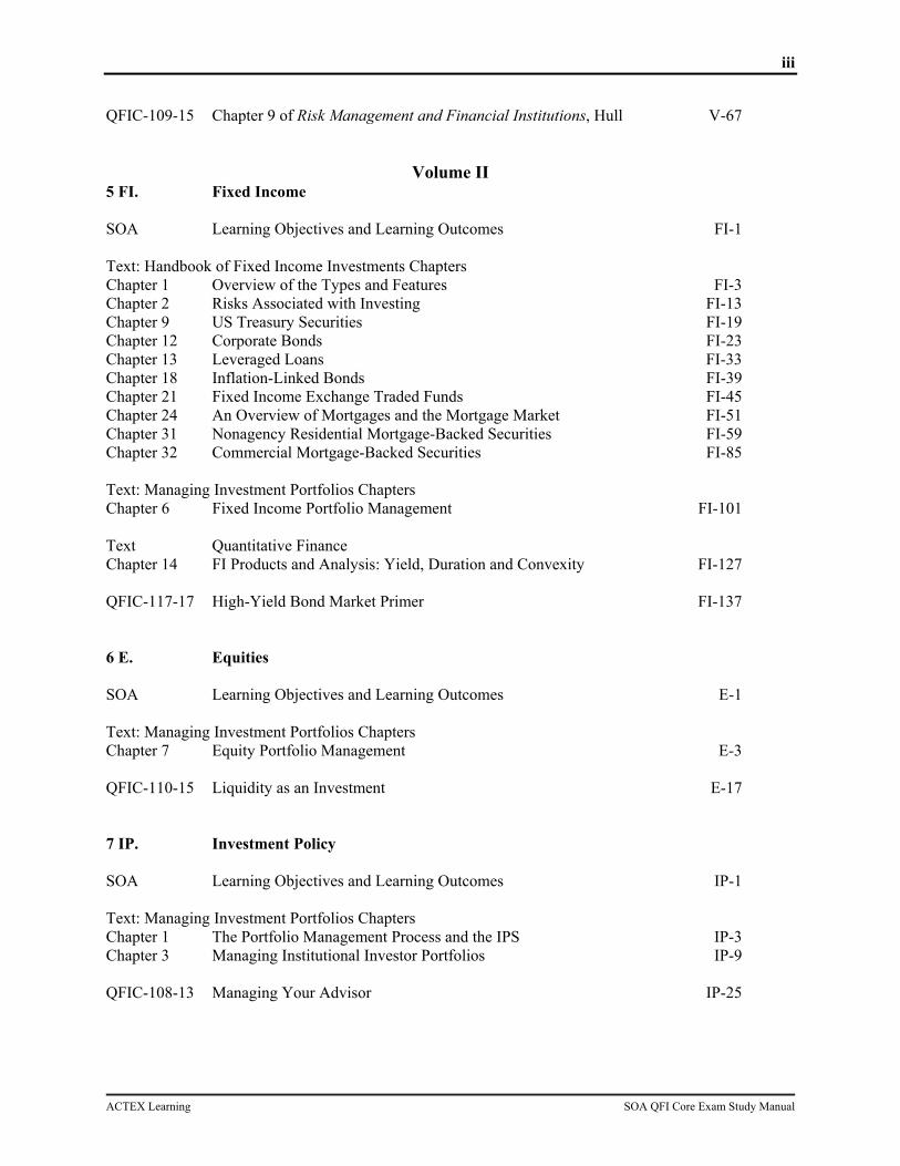
QFIC-109-15 Chapter 9 of Risk Management and Financial Institutions, Hull V-67

Volume II 5 FI. Fixed Income SOA Learning Objectives and Learning Outcomes FI-1 Text: Handbook of Fixed Income Investments Chapters Chapter 1 Overview of the Types and Features FI-3 Chapter 2 Risks Associated with Investing FI-13 Chapter 9 US Treasury Securities FI-19 Chapter 12 Corporate Bonds FI-23 Chapter 13 Leveraged Loans FI-33 Chapter 18 Inflation-Linked Bonds FI-39 Chapter 21 Fixed Income Exchange Traded Funds FI-45 Chapter 24 An Overview of Mortgages and the Mortgage Market FI-51 Chapter 31 Nonagency Residential Mortgage-Backed Securities FI-59 Chapter 32 Commercial Mortgage-Backed Securities FI-85 Text: Managing Investment Portfolios Chapters Chapter 6 Fixed Income Portfolio Management FI-101 Text Quantitative Finance Chapter 14 FI Products and Analysis: Yield, Duration and Convexity FI-127 QFIC-117-17 High-Yield Bond Market Primer FI-137 6 E. Equities SOA Learning Objectives and Learning Outcomes E-1 Text: Managing Investment Portfolios Chapters Chapter 7 Equity Portfolio Management E-3 QFIC-110-15 Liquidity as an Investment E-17 7 IP. Investment Policy SOA Learning Objectives and Learning Outcomes IP-1 Text: Managing Investment Portfolios Chapters Chapter 1 The Portfolio Management Process and the IPS IP-3 Chapter 3 Managing Institutional Investor Portfolios IP-9 QFIC-108-13 Managing Your Advisor IP-25

iv


8 AA. Asset Allocation SOA Learning Objectives and Learning Outcomes AA-1 Text: Managing Investment Portfolios Chapters Chapter 5 Asset Allocation AA-3 QFIC-111-16 Stop Playing with Your Optimizer AA-25 QFIC-112-16 Risk Factors as Building Blocks for Portfolio Diversification AA-29 PP. Practice Problems Practice Problems PP-1

SOA Learning Objectives and Learning Outcomes SC-1


Topic 1: Stochastic Calculus SOA Learning Objectives and Learning Outcomes

I. Learning Objectives

A. "The candidate will understand the fundamentals of stochastic calculus as they apply to option pricing."

II. Learning Outcomes

A. "The Candidate will be able to:

1. "Understand and apply concepts of probability and statistics important in mathematical finance

2. "Understand the importance of the no-arbitrage condition in asset pricing

3. "Understand Ito’s integral and stochastic differential equations

4. "Understand and apply Ito's Lemma

5. "Understand and apply Jensen’s Inequality

6. "Demonstrate an understanding of the option pricing techniques and theory for equity and interest rate derivatives

7. "Demonstrate understanding of the differences and implications of real-world versus risk-neutral probability measures.

8. "Define and apply the concepts of martingale, market price of risk and measures in single and multiple state variable contexts.

9. "Understand and apply Girsanov’s theorem in changing measures.

10. "Understand the Black Scholes Merton PDE (partial differential equation).

SC-2 SOA Learning Objectives and Learning Outcomes


Quantitative Finance Chapter 5 SC-3


Quantitative Finance Paul Wilmott

Chapter 5 Elementary Stochastic Calculus

I. Introduction

A. Random nature of financial markets requires randomness in mathematical tools, thus stochastic calculus

B. Author attempts to be not too technical, avoiding excessive rigor

C. Wants reader to:

1. Understand technical terms

2. Be able to use the stochastic techniques

II. A motivating example

A. Coin toss

1. Heads you win $1

2. Tails you pay $1

3. Ri is the random amount, +1 or -1, for the i-th toss

a. Expectations of Ri

i. E[Ri] = 0, expected value of any toss is 0

ii. [ ] = 1, second moment = 1

iii. E[RiRj] = 0, each toss is independent, past has no impact on future

4. Si is the total amount won up to and including the i-th toss

a. = ∑

b. Expectations of Si

i. E[Si] = 0, cumulative expected value of the tosses is 0

ii. [ ] =

iii. Dependent upon what has happened in previous tosses

SC-4 Quantitative Finance Chapter 5


c. Conditional Expectation

i. E[Si | R1, …Ri-1] = Si-1

a) Expected value of cumulative winnings for the next roll is the same as the current cumulative winnings

III. The Markov property

A. The Markov property - “The expected value of the random variable Si conditional upon all of the past events only depends on the previous value Si-1”

B. Random walk has no “memory” other than where it is currently

1. No Memory – it does not matter the path taken to get to Si-1, all that matters is that the random variable is at Si-1, as if the past was forgotten or if there is no memory of how it got to its state at Si-1

C. Not all random variables have the Markov property

D. Generalization of Markov – If only have information through Sj, 1 ≤ j < i, then estimate of Si is based only on Sj

E. Financial models

1. Most have Markov property

2. Some have small amount of memory

3. A few are totally path dependent, all steps to get to current point matter

IV. The martingale property

A. Martingale property – “conditional expectation of your winnings at any time in the future is just the amount you already hold”

1. E[Si | Sj, j < i] = Sj

a. Here j is the current time, and i is some future time

V. Quadratic variation

A. Definition of quadratic variation for the random walk

1. ∑ ( − )

B. As win/lose 1 after each toss, |Sj – Sj-1| = 1

C. Therefore, quadratic variation is equal to i

1. ∑ ( − ) =



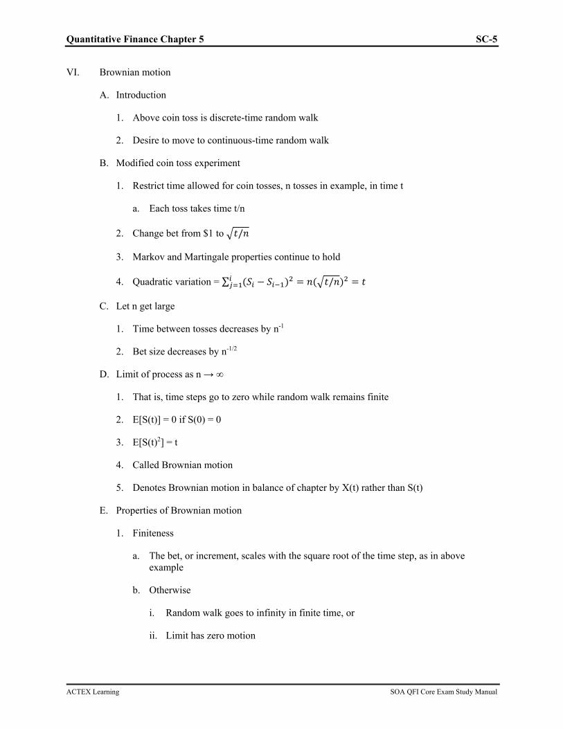
VI. Brownian motion

A. Introduction

1. Above coin toss is discrete-time random walk

2. Desire to move to continuous-time random walk

B. Modified coin toss experiment

1. Restrict time allowed for coin tosses, n tosses in example, in time t

a. Each toss takes time t/n

2. Change bet from $1 to /

3. Markov and Martingale properties continue to hold

4. Quadratic variation = ∑ ( − ) = ( / ) =

C. Let n get large

1. Time between tosses decreases by n-1

2. Bet size decreases by n-1/2

D. Limit of process as n → ∞

1. That is, time steps go to zero while random walk remains finite

2. E[S(t)] = 0 if S(0) = 0

3. E[S(t)2] = t

4. Called Brownian motion

5. Denotes Brownian motion in balance of chapter by X(t) rather than S(t)

E. Properties of Brownian motion

1. Finiteness

a. The bet, or increment, scales with the square root of the time step, as in above example

b. Otherwise

i. Random walk goes to infinity in finite time, or

ii. Limit has zero motion



2. Continuity

a. The path has no discontinuities

b. Brownian motion is the continuous-time random walk, the limit of the discrete-time coin toss example

3. Markov

a. “the conditional distribution of X(t) given information up until τ < t depends only on X(τ)”

i. Information means the values of X previous to and including X(τ) 4. Martingale

a. “Given information up until τ < t the conditional expectation of X(t) is X(τ)”

5. Quadratic variation

a. When time 0 to time t is divided with n+1 partition points, ti = i t /n, then b. ∑ ( − ( )) →

i. “almost surely”

6. Normality

a. With finite increments tj-1 to tj, X(tj) – X(tj-1) is normally distributed

b. Mean = 0 and variance is time increment tj - tj-1

7. Brownian motion is defined by the above six properties

a. Brownian motion is important in financial models

b. X(t) is a random walk process with time steps approaching 0 and is called Brownian motion

VII. Stochastic integration

A. Define stochastic integral as

1. ( ) = ( ) ( ) = lim→ ∑ ( )( − ( ))

a. tj = jt/n

B. Important points about the definition

1. Function f(t) is evaluated at the left-hand point in the summation, i.e. tj-1



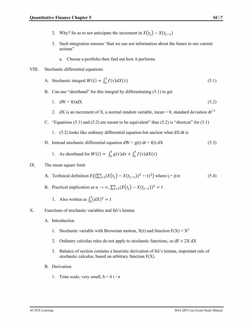
2. Why? So as to not anticipate the increment in − ( )

3. Such integration ensures “that we use not information about the future in our current actions”

a. Choose a portfolio then find out how it performs

VIII. Stochastic differential equations

A. Stochastic integral ( ) = ( ) ( ) (5.1)

B. Can use “shorthand” for this integral by differentiating (5.1) to get

1. dW = f(t)dX (5.2)

2. dX is an increment of X, a normal random variable, mean = 0, standard deviation dt1/2

C. “Equations (5.1) and (5.2) are meant to be equivalent” thus (5.2) is “shortcut” for (5.1)

1. (5.2) looks like ordinary differential equation but unclear what dX/dt is

D. Instead stochastic differential equation dW = g(t) dt + f(t) dX (5.3)

1. As shorthand for ( ) = ( ) + ( ) ( )

IX. The mean square limit

A. Technical definition [(∑ ( − ( )) − ) ] where tj = jt/n (5.4)

B. Practical implication as n → ∞, ∑ ( − ( )) =

1. Also written as ( ) =

X. Functions of stochastic variables and Ito’s lemma

A. Introduction

1. Stochastic variable with Brownian motion, X(t) and function F(X) = X2

2. Ordinary calculus rules do not apply to stochastic functions, so dF ≠ 2X dX

3. Balance of section contains a heuristic derivation of Ito’s lemma, important rule of stochastic calculus, based on arbitrary function F(X)

B. Derivation

1. Time scale, very small, h = δ t / n



2. Approximate F(X(t+h)) with Taylor series

a. ( + ℎ) − ( ) = ( + ℎ) − ( ) ( ) + ( + ℎ) −( ) ( ) + ⋯

b. Sum the series of time steps differences to time t + nh

c. ( + ℎ) − ( ) + ( + 2ℎ) − ( + ℎ) + ⋯ + ( + ℎ) −( + ( − 1)ℎ) = ∑ ( ( + ℎ) − ( + ( − 1)ℎ)) ( + ( − 1)ℎ) +( ) ∑ ( + ℎ) − ( + ( − 1)ℎ) + ⋯

i. Above uses approximation good enough for accuracy desired of

a) ( + ( − 1)ℎ) = ( )

ii. RHS of c. simplifies to F(X(t + nh)) – F(X(t) = F(X(t + δ t)) – F(X(t))

iii. First term of LHS of c. is

iv. Second term of LHS of c. is ( )

d. Result is ( + ) − ( ) = ( ) ( ) + ( )

3. Extend result from time 0 to time t

a. ( ) = (0) + ( ) ( ) + ( )

i. Integral version of Ito’s Lemma

b. Usually written as a stochastic differential equation

i. Ito’s Lemma = + (5.5)

a) More general results of Ito’s Lemma are show below

4. Example of Use of Ito’s Lemma

a. F = X2

b. dF/dX = 2X and d2F/dX2 = 2, assume standard derivatives

c. Result by Ito’s Lemma, dF = 2X dX + (1/2)2dt = 2X dX + dt

i. Not the same as if F were deterministic



d. Integral form = ( ) = (0) + 2 + 1 = 2 +

i. Rearranging, = −

XI. Interpretation of Ito’s Lemma

A. Lemma important in pricing options

B. Figure 5.4 shows random stock price movement and option prices based on that stock price movement

C. Stock price follows stochastic differential equation dS = μ S dt + σ S dX

D. Maybe option value, V(S, t) follows a stochastic differential equation dV = ____dt + ___dX?

E. Ito will help fill in the blanks

XII. Ito and Taylor

A. Seeking intuition behind Ito’s lemma

B. Simple Taylor series expansion of F with small change in X, dX

1. ( + ) = ( ) + + ( )

2. ( + ) − ( ) is change in F, or dF, and

3. = ( ) + ( )

a. Very similar to (5.5) and Ito

b. Difference, (5.5) has “dt” while above has “dX2”

4. And without “rigor”, dX2 = dt (5.6)

C. Generalize the stochastic differential equation

1. dS = a(S) dt + b(S) dX (5.7)

a. a(S), b(S) functions of S, although in some formulas Wilmott uses simply a, b, dropping (S)

b. dX the Brownian motion increment

c. S thus has deterministic time element, dt, and a random element, dX



2. Another function of S, V(S), what is dV?

a. “Cheat by using Taylor series with dX2 = dt”, replacing “F” with “V” and “X” with “S”

i. = + (5.7a)

ii. Random element in this equation is not shown directly, i.e. no dX term, but is inside of the dS term.

b. Equation using the pure random term dX

i. = ( ) + ( ) + ( )

ii. Derive from 2.a.i and using equation (5.7), gathering the dt terms

XIII. Ito in higher dimensions

A. In finance, many functions of deterministic t and stochastic S, and the coefficients of stochastic differential equation of S are functions of both S and t, a(S, t) and b(S, t). The derivative V(S, t) a function of both S and t.

1. dS = a(S, t) dt + b(S, t) dX

2. = + + , the general version of Ito with a single random

variable

B. Function of two or more random variables V(S1, S2, t) with correlated random increments dX1, dX2

1. dS1 = a1(S1, t) dt + b1(S1, t) dX1

2. dS2 = a2(S2, t) dt + b2(S2, t) dX2

3. Rules of thumb, = , = , =

4. Ito’s Lemma result

a. = + + + + + (5.9)

XIV. Some pertinent examples

A. Section Beginning

1. General form of stochastic differential equation of interest, dS = ____dt + ___dX

a. Deterministic piece with dt and random piece with dX



b. What functions to use with each piece? Different functions for different financial instruments

B. Brownian motion with drift

1. dS = μ dt + σ dX

a. μ is the drift, or movement away from a mean of 0

b. Can go negative, shown in Figure 5.5, not good for some financial values such as equity values or interest rates (text written before the 2007-09 financial crisis and central banks causing interest rates to go negative)

c. Integrate SDE to get S(t) = S(0) + μt + σ(X(t) – X(0))

C. The lognormal random walk

1. dS = μSdt + σSdX (5.10)

a. Both drift and randomness multiplied by S

b. With S(0) > 0, S(t) cannot be negative

2. Define F(S) = log S then

a. = + = ( + ) − = − +

i. As = and = −

b. -∞ < Log S < ∞, but cannot reach the limit in finite time, and S cannot reach either 0 or ∞

3. Integral form: ( ) = (0) ( ( ) ( )) 4. For V(S, t), with a lognormal random walk, using Ito

a. = + + (5.11)

D. A mean-reverting random walk

1. dS = (ν – μS)dt + σ dX

a. Negative coefficient of S implies large S will tend to move down, small S will tend to move up, “reverting to the mean”

b. S does not have to stay positive

2. Mean reverting often used for interest rates



3. Vasicek model for short-term interest rates, use “r” rather than “S” E. And another mean-reverting random walk

1. Adjust the random term of the prior SDE3e

2. dS = (ν – μS)dt + σS1/2 dX

a. When S gets close to 0, randomness decreases

3. Define F = S1/2, find SDE for F

a. Ito’s Lemma result = +

i. Why σ2S in the dt term? It is the square of the coefficient of the random dX term in the SDE for S

ii. Note similar usage in the formula at the bottom of page 135

b. Derivatives of F

i. = / , = −

c. Substitute derivatives and dS into Ito

i. = / [( − ) + ] + [− ]

ii. = − + −

iii. = ( − ) +

a) Constant random term, messy drift term

b) Drift term is problematic at F = S = 0

4. Find F(S) such that drift term is 0

a. Need ( − ) + = 0

i. Applied Ito to dS above

b. Resulting equation =

i. A is any constant

ii. If ν is large enough, random walk avoids a value of 0



XV. Summary

A. With Ito’s Lemma, can handle functions of a random variable

B. Asset S with a stochastic differential equation, then can price derivatives of S

C. Need to be able to use the Ito tool

XVI. Time Out – Learn by Using

A. “Stochastic differential equations are like recipes for generating random walks”

B. “If you have some quantity, let’s call it S, that follows such a random walk, then any function of S is also going to follow a random walk.”

C. “The question then becomes ‘What is the random walk for this function of S?’ That is, what is its recipe, or what is its stochastic differential equation?”

D. “Applying something very like Taylor series but with two tricks”

1. One – in Taylor expansion, “only keep terms of size dt or bigger (dt1/2)”

2. Two – Replace dX2 with dt



Quantitative Finance Paul Wilmott

Chapter 6 The Black-Scholes Model

I. Introduction

A. "Most important chapter in the book"

B. Building blocks of derivative theory

1. Delta hedging

2. No arbitrage

C. While Black-Scholes (B-S) assumptions can be incorrect, model is important in practice and theory

II. A Very Special Portfolio

A. Notation: Value of an option:

1. V(S, t; σ, μ; E, T; r)

a. S and t are variables

i. S spot price of underlying asset

ii. t current time or today's date

b. σ, μ are parameters of the asset price

i. σ: annualized volatility or standard deviation

ii. μ: annualized growth rate, however we know this does not impact the price of the option

c. E and T are details of the option contract

i. E strike price (note different notation than other authors)

ii. T time of expiry of contract

d. r is parameter of the currency of the option

e. Generally, will use V(S, t) or V if others clear from context

B. Notation: Value of Portfolio of one long option and a short position of Δ in underlying:

1. Π = V(S, t) - ΔS (6.1)



C. Assume price of underlying asset follows lognormal random walk

1. dS = μS dt + σS dX

a. Change in price of the underlying is mean return on asset for time period of dt plus the volatility of the underlying time the value of the underlying times dX

b. X(t) is a Brownian motion

i. Properties of Brownian motion p121-122 (these pages are not on syllabus but they can assist understanding)

a) Finiteness - increment scales with square root of time step

b) Continuity - Brownian motion is continuous-time limit of discrete time random walk

c) Markov - Conditional X(t) given prior info until τ < t depends only on X(τ)

d) Martingale - Given info until τ < t, conditional expectation of X(t) is X(τ)

e) Quadratic Variation - sum of squares of differences of X(t), of [X(ti) - X(ti-1)] approach t, on a 0 to t time range

f) Normality - differences of [X(ti) - X(ti-1)] are normally distributed with mean zero and variance tj-tj-1

D. Change in value of portfolio

1. dΠ = dV - ΔdS

2. From Ito's Lemma

a. = + +

b. For review of Ito's Lemma, see Neftci Chapter 10

3. Then change in value of portfolio is

a. Π = + + − ∆ (6.2)

i. Deterministic terms of dt

ii. Random or stochastic terms of dS, the risk in the portfolio

III. Elimination of Risk: Delta Hedging

A. If random term ( − ∆) = 0, then risk eliminated

B. If Δ = ∂V/∂S, then risk eliminated (6.3)



C. Hedging - "any reduction in randomness"

D. Delta-hedging - "exploiting correlation between two instruments"

E. Dynamic hedging strategy - as delta changes with time, the delta-hedge must be adjusted or rebalanced, theoretically continuously.

IV. No Arbitrage

A. Given Δ above, then Π = ( + ) (6.4)

1. No risk in dΠ as no dS term in above equation

2. No risk implies portfolio should earn risk free rate using no-arbitrage principle

3. dΠ = rΠ dt (6.5)

V. The Black-Scholes Equation

A. Given

1. Π = ( + )

2. dΠ = rΠ dt

3. Π = V(S, t) - ΔS

4. Δ = ∂V/∂S,

B. Then, substituting 4 into 3, and the result into right hand side of 2, equating 1 and 2, dividing all than by dt and rearranging,

1. + + − = 0 (6.6)

C. Above equation is the B-S equation

1. A linear parabolic partial differential equation

a. Linear - If have two solutions, then the sum of the two solutions is also a solution

b. Parabolic - related to diffusion equation

c. Relatively easy to solve numerically

D. Why no "drift" term or mean or expected return parameter in B-S?

1. Mathematical argument - μ dropped out with dS term

2. Economic argument - If can hedge risk of option with underlying, there should be no reward for such a portfolio, it should earn the risk free rate



3. Option can be replicated with cash and buying/selling the underlying

4. Complete market - one which an option can be replicated with the underlying

a. Transaction costs lead to incomplete markets

5. Time Out

a. At a time-step before expiry, δt, the value of the option appears to be the "moneyness" of the option plus, if in the money, a time value that looks like an interest earning on the strike price for that time-step

VI. The Black-Scholes Assumptions

A. Wilmott lists most important assumptions and discusses some generalizations

B. Underlying follows lognormal random walk

1. To find solutions

a. Random term must be proportional to S

b. σ does not need to be constant but needs to be proportional to time

c. Elimination of arbitrage eliminates μ term from solution

C. Risk-free interest rate is a known function of time

1. Restriction helps find solutions

2. If constant formula easier

3. Reality - risk-free rate is not known and it is stochastic

D. No dividends on the underlying

1. Restriction to be dropped shortly

E. No transaction costs

1. Not realistic

2. Trade-off between transaction costs and frequency of rebalancing

F. No arbitrage opportunities

1. Exist in reality

2. Rule out model-dependent arbitrage



VII. Final Conditions

A. B-S equation independent on type of option, strike and expiry

B. These distinctions handled by "final conditions" or the payoff at expiry

1. Heaviside function, (using Greek capital eta as I cannot find the symbol Wilmott uses)

a. Ή(·)

i. Zero when argument is zero

ii. One when argument is positive

2. Examples of Final Conditions

a. Call option V(S, T) = max(S - E, 0)

b. Put option V(S, T) = max(E - S, 0)

c. Binary Call V(S, T) = Ή(S - E)

d. Binary Put V(S, T) = Ή(E - S)

C. Observe that S and ert satisfy the B-S equation

1. Let V = S,

a. Then

i. ∂V/∂S = 1

ii. ∂2V/∂S2 = 0

iii. ∂V/∂t = 0

b. Substituting into B-S, rS-rS = 0 satisfying the equation

2. Similar process letting V = ert

VIII. Options on Dividend-Paying Equities

A. Simple modification of non-dividend paying B-S equation

1. Let D = continuous dividend rate

2. D S dt = dividend paid in time dt

3. Holding Δ shares, dividend is D ΔS dt

B. Generalized equation is

1. + + ( − ) − = 0 (6.7)



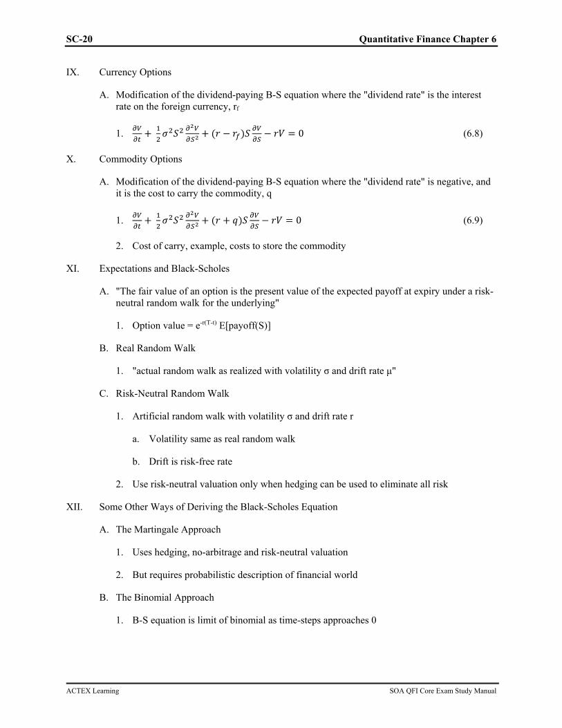
IX. Currency Options

A. Modification of the dividend-paying B-S equation where the "dividend rate" is the interest rate on the foreign currency, rf

1. + + ( − ) − = 0 (6.8)

X. Commodity Options

A. Modification of the dividend-paying B-S equation where the "dividend rate" is negative, and it is the cost to carry the commodity, q

1. + + ( + ) − = 0 (6.9)

2. Cost of carry, example, costs to store the commodity

XI. Expectations and Black-Scholes

A. "The fair value of an option is the present value of the expected payoff at expiry under a risk-neutral random walk for the underlying"

1. Option value = e-r(T-t) E[payoff(S)]

B. Real Random Walk

1. "actual random walk as realized with volatility σ and drift rate μ"

C. Risk-Neutral Random Walk

1. Artificial random walk with volatility σ and drift rate r

a. Volatility same as real random walk

b. Drift is risk-free rate

2. Use risk-neutral valuation only when hedging can be used to eliminate all risk

XII. Some Other Ways of Deriving the Black-Scholes Equation

A. The Martingale Approach

1. Uses hedging, no-arbitrage and risk-neutral valuation

2. But requires probabilistic description of financial world

B. The Binomial Approach

1. B-S equation is limit of binomial as time-steps approaches 0



C. CAPM/Utility

1. Uses risk and reward (return) to optimally allocate portfolio

2. Including options in framework does not increase risk/reward as options are simply functions of the underlyings

3. Market completeness

XIII. No Arbitrage in the Binomial, Black-Scholes and 'Other' Worlds

A. With binomial and B-S, proper choice of Δ can eliminate risk

B. Not so with other models

1. Trinomial model example

a. Effectively trying to solve two equations with the one unknown, Δ

C. Footnote 4, page 150, Wilmott makes an important point that these are models, not reality. However, they can be a good starting point, not an ending point as models can be "wrong'

XIV. Forwards and Futures

A. Forwards

1. S is fixed delivery price

2. Portfolio Π = V(S, t) - ΔS, then as above, choose Δ = ∂V/∂S, eliminate risk, apply no arbitrage, result is B-S equation

a. At expiry, V(S, T) = S - S

b. Solution to PDE is V(S, t) = S(t) - S e-r(T-t)

c. At initiation, V(S, 0) = 0, no price is needed to enter a forward, then S = S erT)

3. Verify B-S holds, Let V = S(t) - S e-r(T-t)

a. Then

i. ∂V/∂S = 1

ii. ∂2V/∂S2 = 0

iii. ∂V/∂t = - r S e-r(T-t)

b. Substituting into B-S, - r S e-r(T-t) + rS - r(S - S e-r(T-t)) = 0 satisfying the equation



XV. Futures Contracts

A. F(S, t) notation for futures price

1. F(S, t) = 0 for all t due to daily settlement of contract

2. Portfolio long future and short Δ shares of stock

a. Π = 0 - ΔS

b. dΠ = dF - ΔdS, with dF being the continuous settlement cash flow

c. Π = + + − Δ

d. Make dS terms go away by setting Δ = ∂F/∂S

e. Eliminate risk by dΠ = rΠdt

3. Result is not a B-S form, + + = 0

a. Final condition, F(S, T) = S as futures price and underlying must have the same value at maturity

b. General solution F(S, t) = Ser(T-t)

4. Note, when interest rates are a known function of time, forward and futures prices are the same

a. Differences when rates are stochastic

XVI. Options on Futures

A. Futures price

1. = ( )

B. V(S, t) = ( , )

1. + − = (6.10)

Introduction to the Mathematics of Financial Derivatives Chapter 1 SC-23


An Introduction to the Mathematics of Financial Derivatives, 3rd Edition Ali Hirsa, Salih Neftci

Chapter 1 Financial Derivatives - A Brief Introduction

I. Introduction

A. Book discusses logic behind asset pricing

B. Chapter discusses two building blocks of financial derivatives, options and forwards

C. Complicated derivatives can be decomposed into simpler derivatives

D. Study manual author note: Much of the material in this chapter is a review from Exams FM and MFE

II. Definition

A. Derivative security or contingent claim: "A financial contract is a derivative security, or a contingent claim, if its value at expiration date T is determined exactly by the market price of the underlying cash instrument at time T"

B. Notation

1. T: expiration date of derivative

a. After this date the derivative contract no longer exists

2. F(T): price of derivative asset

3. ST: price of the relevant cash instrument, called the "underlying asset", at time T

4. F(t) and F(St, t): price of derivative on underlying St at time t

5. dt : Yield of payout on a derivative

III. Types of Derivatives

A. Introduction

1. Three general types of derivatives

a. Futures and forwards: basic building block

b. Options: basic building block

c. Swap: hybrid security that can be decomposed into set of forwards and options

SC-24 An Introduction to the Mathematics of Financial Derivatives Chapter 1


2. Five main groups of underlying assets

a. Stocks

i. Claims on returns from production of goods/services

b. Currencies

i. Not direct claims on real assets

c. Interest Rates

i. Not really assets, so a notional asset needs to be determined

d. Indexes

i. E. G. S&P 500, FT-SE100

ii. Need notional amount

e. Commodities

i. Not financial assets, can be physically purchased and stored

B. Cash-and-Carry Markets

1. Cash-and-Carry are an alternative to holding a forward/futures contract on commodity

a. Buy directly in cash markets or buy indirectly using forward/futures

i. At expiration, in either case, the long position holds the commodity

2. Examples: gold, silver, currencies, T-bonds

3. Features of Cash-and-Carry Market

a. Borrow at risk-free rates by collateralizing the underlying

b. Buy and store the product

c. Insure it until expiration of derivative contract

4. Additional property

a. Information about future conditions, supply/demand, etc., should not change the spread between cash and futures prices

i. New information changes the price of both by about the same amount



C. Price-Discovery Markets

1. Differences from Cash-and-Carry

a. Commodity is perishable or

b. Commodity does not yet exist, e.g. spring wheat

2. Features

a. Not physically possible to buy commodity and store until expiration date of derivative

b. No cash market yet exists, e.g. crop has not yet been harvested

3. Impact of Information

a. Future supply/demand cannot influence cash price

b. Such information will influence, and thus can be discovered, in the futures market

D. Expiration Date

1. Value of futures contract at expiry should be equal to the value of the underlying

a. F(T) = ST (1.1)

2. Value of F(t), t < T, is not necessarily equal to St

IV. Forwards and Futures

A. Forward

1. Forward: "a forward contract is an obligation to buy (sell) an underlying asset at a specified forward price on a known date"

2. Review of payoff diagrams, pages 4,6

B. Futures

1. Similar to forwards in that they are both obligations for settlement at a specified future date of an underlying

2. Differences between forwards and futures

a. Where Traded

i. Futures: on formal, public exchanges

ii. Forwards: private contracts in the OTC market (over the counter)



b. Credit Risk

i. Futures: cleared through an exchange designed to reduce default risk

ii. Forwards: private contracts so risk depends on the credit quality of the counterparty

c. Mark-to-Market

i. Futures: Daily, effectively settled daily with a new contract created

a) Daily profit/loss recorded

ii. Forwards: no mark-to-market

C. Repos, Reverse Repos, and Flexible Repos

1. Repos

a. Definition

i. "A repurchase agreement, also known as a repo, is a transaction in which one party sells securities to another party in return for cash, with an agreement to repurchase equivalent securities at an agreed upon price and on an agreed upon future date."

a) You could think of this as a loan with the difference between the cash amount and the "agreed upon price" as interest on the loan.

i) Securities are the collateral for the loan

ii) This interest amount creates the "repo rate"

b) Alternatively, think of a repo as a spot sale and a forward contract

ii. For seller, called repo

iii. For buyer of security, called reverse repo

iv. Classified as money market instruments

b. Types of repos

i. Overnight: one-day maturity

ii. Term: specified maturity date other than one-day

iii. Open: no end date

c. Forms of Repo Transactions

i. Specified Delivery



ii. Tri-party

iii. Hold-in-custody

a) Selling party holds security during repo term

2. Flexible Repos

a. A repo with a flexible withdrawal schedule, both in terms of timing and amount

b. Differences from traditional repo

i. "Convexity due to cash withdrawals

ii. "Formal written auction like trade

iii. Additional documentation is necessary for credit protection

iv. Counterparties are typically muni bond issuers

c. Types of flexible repos

i. Secured

a) Municipality receives collateral

i) Treasuries, GNMA, agency MBS, etc.

ii) Collateral comes from a reverse repo

b) Average size 10 - 20 million

ii. Unsecured

a) No collateral but likely higher rate

b) Average size - smaller than secured

V. Options

A. General

1. The right, but not an obligation, to do something

2. Call: "A European-type call option on a security St is the right to buy the security at a preset strike price K. This right may be exercised at the expiration date T of the Option. The call option can be purchased for a price of Ct dollars, the call premium, at time t < T"

3. Put: right to sell



4. Exercise Dates

a. European options: only at expiry

b. American options: exercised at any time, not just the expiration date

5. Reasons traders need to know the value of Ct

a. Estimate of price to trade, especially if traded infrequently

b. Evaluate risk

c. Determine any mispricing for an arbitrage opportunity

B. Some Notation

1. Best to find a formula, or closed form solution, for Ct as a function the underlying

2. Only known formula for Ct is at T

a. Out of the money expiry, ST < K (1.2)

i. Implies CT = 0 (1.3)

b. In-the-money expiry, ST > K (1.4)

i. Implies CT = ST - K (1.5)

c. CT = max(ST - K, 0) (1.6)

i. Formula for CT shows options are non-linear

3. Figures 1.3 and 1.4, page 8, graph values of call options at times before expiry

VI. Swaps

A. General

1. Swap: "A swap is the simultaneous selling and purchasing of cash flows involving various currencies, interest rates, and a number of other financial assets"

2. Method to price swaps is to decompose swap into forwards and options, price the forwards and options, sum these prices to get price of swap

B. A Simple Interest Rate Swap

1. Notional principals



2. Two counterparties for interest rate swap

a. Party A to pay fixed on notional, receive floating on notional

b. Party B to received fixed on notional, pay floating on notional

c. Each period, payments are netted, net payment is essentially the interest rate differential times the notional principal

d. Based on comparative advantage, each party should secure lower rates

e. Swap dealer earns a fee for bringing parties together

3. Basket of forward contracts will replicate the cash flow helping to value the swap

C. Cancelable Swaps

1. Definition

a. "A cancelable swap is a swap where one or both parties has the right but not the obligation to cancel the swap before its maturity."

i. Dates to cancel the swap specified in the contract

2. Types of Cancelable Swaps

a. Callable Swap

i. Payer of fixed rate has the option

a) On specified dates

b) At cancelation, payer

i) Pays present value of future payments

ii) Receives a premium

b. Puttable Swap

i. Receiver of fixed rate has the option

a) On specified dates

c. Vanilla Swap can be "closed out"

i. By paying net present value of future payments

3. Uses of Cancelable Swaps

a. Use with callable bonds



b. Use as asset/liability hedges

i. Specifically, when liabilities have prepayment options

Quantitative Finance & Investments Core Study Manual Core SAMPLE.pdf · ACTEX Learning New...

Documents

Transcript of Quantitative Finance & Investments Core Study Manual Core SAMPLE.pdf · ACTEX Learning New...