Software Tip

Quantitative EMG analysis inLabChart

Quantitative EMG analysis in LabChart:

Area under curve

Measuring area under the rectified EMG waveform is standard practice for quantifying myoelectricsignals during muscle contraction. LabChart can do this in two ways:

Part I - Use the Peak Analysis module on Smoothed EMG data (easiest method);

Part II - Compute the integral of raw windowed EMG data and add to the Data Pad for analysis.

Part I - Easy solution using Peak Analysis

Smoothing the EMG waveform 1. Create a new channel from Setup and rename it ‘Smoothed EMG’ (figure 1). Under Calculation in thefar right column, select Smoothing for the newly created channel.

Figure 1: From the top menu select: Setup->Channel Settings.

Page 1/16

Software Tip

2. Apply a Triangular smoother to the raw EMG data with a window width of 301 samples (figure 2).

Figure 2: A triangular window with a width of 301 samples (for a sampling rate of 1 kHz)produces significant EMG smoothing, such that individual spikes are no longer present.

3. A new channel should now appear below the original recorded EMG signal (figure 3).

Page 2/16

Software Tip

Figure 3: Top trace: grip force recording. Middle trace: raw EMG data.Lower trace: smoothed EMG data.

Detect EMG event 4. Open Peak Analysis settings from the top menu (figure 3). In the analysis type, choose ‘General –Unstimulated’ for voluntary muscle activity or, if electrical stimulation was used to elicit the EMGactivity, choose ‘Evoked Response’. Make sure the source channel is set to the smoothed EMG signal and apply to a data selection or entirechannel as necessary. The preset detector ‘General – Peak After Threshold’ works best for EMG data.Although it cannot cope with baseline drift, it allows single-peak detection when the peak region isquite noisy.

Page 3/16

Software Tip

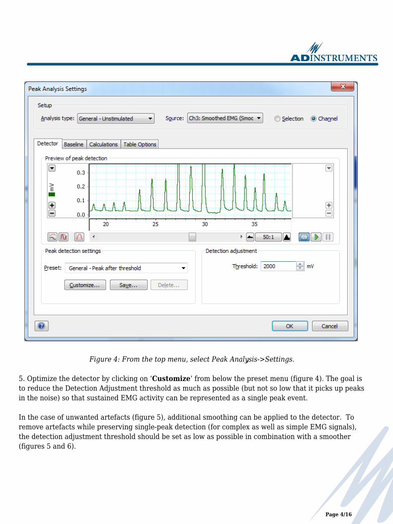
Figure 4: From the top menu, select Peak Analysis->Settings. 5. Optimize the detector by clicking on ‘Customize’ from below the preset menu (figure 4). The goal isto reduce the Detection Adjustment threshold as much as possible (but not so low that it picks up peaksin the noise) so that sustained EMG activity can be represented as a single peak event. In the case of unwanted artefacts (figure 5), additional smoothing can be applied to the detector. Toremove artefacts while preserving single-peak detection (for complex as well as simple EMG signals),the detection adjustment threshold should be set as low as possible in combination with a smoother(figures 5 and 6).

Page 4/16

Software Tip

Figure 5: Detection on unwanted signal – further optimization required.

Figure 6: Use smoothing in combination with a detection threshold. EMG analysis 6. In Peak Analysis Settings, under the Table Options tab (figure 7), select Height and Peak Area.

Page 5/16

Software Tip

Open the Table View from the Peak Analysis menu (figure 8); the data for peak amplitudes will bedisplayed, as well as the area under the curve. If PeakArea values cannot be calculated and are missing from the Table View, detection settings mayneed to be optimized further. In any case, using the Analysis View (top left of figure 8) is helpful forchecking the accuracy of peak detection.

Figure 7: Table View options: height and area are probably most applicable to EMG data –but other parameters may be useful too such as width, onset time, and time to peak.

Page 6/16

Software Tip

Figure 8: Diagnosing the detected peaks using Table View and Analysis View. Troubleshooting PeakArea calculations 7. Open the Analysis and Table Views from the Peak Analysis menu. Clicking on a row in the Table Viewthat does not contain a PeakArea value will cause that peak to be displayed in the Analysis View. In the Example shown below using Peak Analysis 1.3.2 (figure 9a) the reason PeakArea is notcalculated in the first entry (highlighted in blue in the Table View) is the end of the peak did not crossthe baseline, due to the onset of a second peak.

Page 7/16

Software Tip

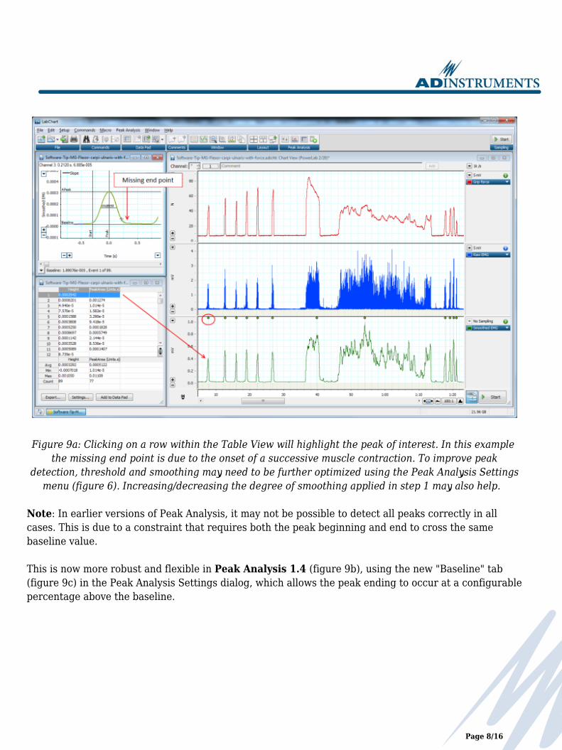
Figure 9a: Clicking on a row within the Table View will highlight the peak of interest. In this example

the missing end point is due to the onset of a successive muscle contraction. To improve peakdetection, threshold and smoothing may need to be further optimized using the Peak Analysis Settings

menu (figure 6). Increasing/decreasing the degree of smoothing applied in step 1 may also help. Note: In earlier versions of Peak Analysis, it may not be possible to detect all peaks correctly in allcases. This is due to a constraint that requires both the peak beginning and end to cross the samebaseline value. This is now more robust and flexible in Peak Analysis 1.4 (figure 9b), using the new "Baseline" tab(figure 9c) in the Peak Analysis Settings dialog, which allows the peak ending to occur at a configurablepercentage above the baseline.

Page 8/16

Software Tip

Figure 9b: Peak Analysis 1.4 with all peaks detected and missing Peak Area calculated.

Page 9/16

Software Tip

Figure 9c: "Baseline" tab in Peak Analysis 1.4 Settings dialog with TStart set to 5% and TEnd set to 3%.

Part II - Computing the integral as a channel calculation

Where Peak Analysis is unable to detect EMG waveform boundaries optimally, you can manuallycompute the area under the rectified EMG curve using Comments and Multiple Add to Data Padfeatures. Create an integral channel 1. Setup menu->Channel Settings (figure 10).

Page 10/16

Software Tip

Figure 10: From the LabChart menu, select Setup->Channel Settings.

2. Integral settings: Set the source channel to the raw EMG data and ensure the reset type is set to NoReset (figure 11).

Page 11/16

Software Tip

Figure 11: Integral Settings Menu. 3. Define EMG ‘windows’ using comments. For each epoch of EMG activity, add a comment to thebeginning of the series by positioning the cursor and right-clicking (or Ctrl-K) followed by ‘addcomment’. Label the comment ‘s’ to denote start. Repeat for the end of the EMG event and label ‘e’ todenote end. Repeat this for all muscle contractions of interest (Figure 12).

Page 12/16

Software Tip

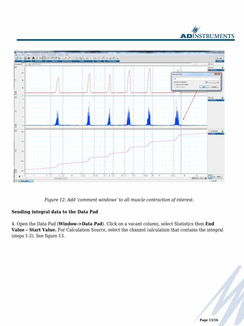
Figure 12: Add ‘comment windows’ to all muscle contraction of interest. Sending integral data to the Data Pad 4. Open the Data Pad (Window->Data Pad). Click on a vacant column, select Statistics then EndValue – Start Value. For Calculation Source, select the channel calculation that contains the integral(steps 1-2). See figure 13.

Page 13/16

Software Tip

Figure 13: Prepare a DataPad column for the next step – multiple add to DataPad. 5. Use Multiple Add to Data Pad (Commands->Multiple Add to Data Pad) to send the integral data(defined by the ‘s’ and ‘e’ boundaries) to the Data Pad. The column previously set up (column 4a) willautomatically compute and display the integral difference between the start and end of the EMG event. Multiple Add to Data Pad

Page 14/16

Software Tip

Figure 14: Multiple Add to Data Pad settings.

6. Find using: comment 7. From channel: any 8. Containing: ‘s’ (without quotation marks) 9. Select to the next comment containing: ‘e’ (without quotation marks) 10. Step through: whole file

11. The Data Pad will now be populated with the absolute integral for each windowed region in the rawEMG data series (figure 15).

Page 15/16

Software Tip

Figure 15: Area under curve for each EMG event.

Page 16/16