Quantitative Description of Robot-Environment Interaction

Using Chaos Theory1

Ulrich Nehmzow Keith Walker

Dept. of Computer Science Department of PhysicsUniversity of Essex Point Loma Nazarene UniversityWivenhoe Park 3900 Lomaland DriveColchester CO4 3SQ San Diego, CA 92106-2899United Kingdom USA

Abstract. Any theory (such as, for example a theory of robot-environment interaction) is dependent upon quanti-tative descriptions of behaviour. In this paper we present experiments on the application of chaos theory to describea robot’s behaviour quantitatively.Computing the Lyapunov exponent of robot trajectories observed in a number of experiments, we find that a changein task influences robot behaviour far more noticeably than a change in environment.

1 Introduction

1.1 Motivation

Research in mobile robotics to date has, with very few exceptions, been based on trial-and-error experimen-tation and the presentation of existence proofs. Task- achieving robot control programs are obtained througha process of iterative refinement, typically involving the use of computer models of the robot, the robot itself,and program refinements based on observations made using the model and the robot. This process is iterateduntil the robot’s behaviour resembles the desired behaviour to a sufficient degree of accuracy. Typically, theresults of these iterative refinement processes are valid within a very narrow band of application scenarios,they constitute “existence proofs”. As such, they demonstrate that a particular behaviour can be achieved,but not how that particular behaviour can in general be achieved for any experimental scenario.

1.2 A Theory of Robot-Environment Interaction

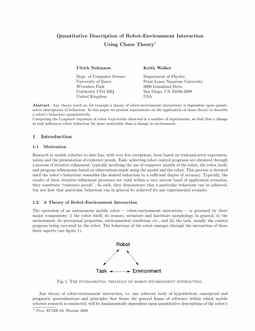
The operation of an autonomous mobile robot — robot-environment interaction — is governed by threemajor components: i) the robot itself, its sensors, actuators and hardware morphology in general, ii) theenvironment, its perceptual properties, environmental conditions etc., and iii) the task, usually the controlprogram being executed by the robot. The behaviour of the robot emerges through the interaction of thesethree aspects (see figure 1).

Fig. 1. The fundamental triangle of robot-environment interaction.

Any theory of robot-environment interaction, i.e. any coherent body of hypothetical, conceptual andpragmatic generalisations and principles that forms the general frame of reference within which mobilerobotics research is conducted, will be fundamentally dependent upon quantitative descriptions of the robot’s1 Proc. ECMR 03, Warsaw 2003

behaviour. While we investigate a general theory of robot-environment interaction in ongoing work at Essexand Point Loma, the purpose of this paper is to introduce the idea that chaos theory can be applied todescribe a robot’s behaviour quantitatively.

1.3 Quantitative Analysis of Robot-Environment Interaction

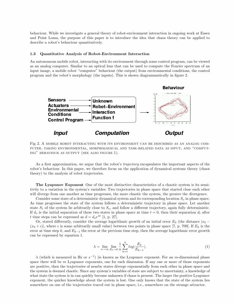
An autonomous mobile robot, interacting with its environment through some control program, can be viewedas an analog computer. Similar to an optical lens that can be used to compute the Fourier spectrum of aninput image, a mobile robot “computes” behaviour (the output) from environmental conditions, the controlprogram and the robot’s morphology (the inputs). This is shown diagrammatically in figure 2.

Fig. 2. A mobile robot interacting with its environment can be described as an analog com-

puter, taking environmental, morphological and task-related data as input, and “comput-

ing” behaviour as output (see also figure 1).

As a first approximation, we argue that the robot’s trajectory encapsulates the important aspects of therobot’s behaviour. In this paper, we therefore focus on the application of dynamical systems theory (chaostheory) to the analysis of robot trajectories.

The Lyapunov Exponent One of the most distinctive characteristics of a chaotic system is its sensi-tivity to a variation in the system’s variables: Two trajectories in phase space that started close each otherwill diverge from one another as time progresses, the more chaotic the system, the greater the divergence.

Consider some state of a deterministic dynamical system and its corresponding location So in phase space.As time progresses the state of the system follows a deterministic trajectory in phase space. Let anotherstate S1 of the system lie arbitrarily close to So, and follow a different trajectory, again fully deterministic.If do is the initial separation of these two states in phase space at time t = 0, then their separation dt aftert time steps can be expressed as d = doe

λt [1, p. 27].Or, stated differently, consider the average logarithmic growth of an initial error E0 (the distance |x0 −

(x0 + ε)|, where ε is some arbitrarily small value) between two points in phase space [7, p. 709]. If Ek is theerror at time step k, and Ek−1 the error at the previous time step, then the average logarithmic error growthcan be expressed by equation 1.

λ = limn→∞

limE0→0

1n

n∑k=1

log| EkEk−1

|. (1)

λ (which is measured in Hz or s−1) )is known as the Lyapunov exponent. For an m-dimensional phasespace there will be m Lyapunov exponents, one for each dimension. If any one or more of those exponentsare positive, then the trajectories of nearby states diverge exponentially from each other in phase space andthe system is deemed chaotic. Since any system’s variables of state are subject to uncertainty, a knowledge ofwhat state the system is in can quickly become unknown if chaos is present. The larger the positive Lyapunovexponent, the quicker knowledge about the system is lost. One only knows that the state of the system liessomewhere on one of the trajectories traced out in phase space, i.e., somewhere on the strange attractor.

The Lyapunov exponent is one of the most useful quantitative measures of chaos, since it will reflectdirectly whether the system is indeed chaotic, and will quantify the degree of that chaos. Also, knowledge ofthe Lyapunov exponents becomes imperative for any analysis on prediction of future states. For example, ina system exhibiting highly chaotic deterministic behaviour (large Lyapunov exponent), predictions within adefined error margin of future system states are only possible for a few time steps ahead. The movement ofa billiard ball in a game of pools is an example of this. On the other hand, for systems exhibiting no or verylittle deterministic chaos (small Lyapunov exponent, for example a pendulum), predicitions within the samedefined error margin are possible for a larger number of time steps.

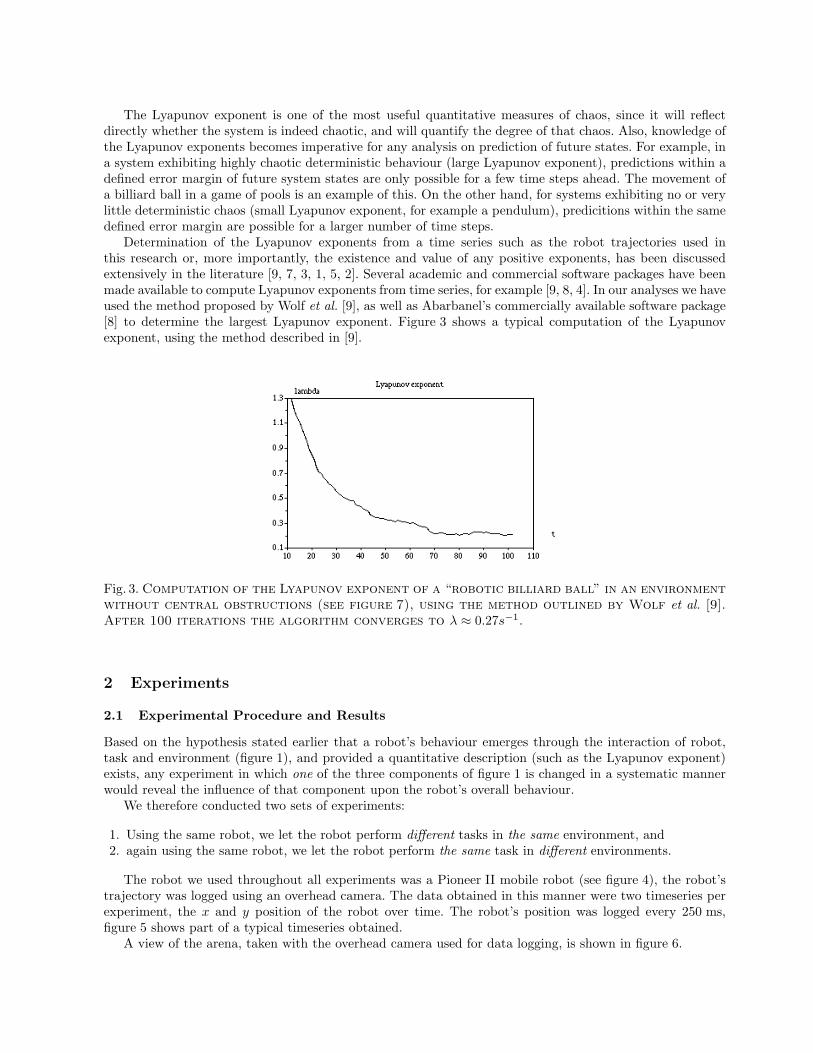
Determination of the Lyapunov exponents from a time series such as the robot trajectories used inthis research or, more importantly, the existence and value of any positive exponents, has been discussedextensively in the literature [9, 7, 3, 1, 5, 2]. Several academic and commercial software packages have beenmade available to compute Lyapunov exponents from time series, for example [9, 8, 4]. In our analyses we haveused the method proposed by Wolf et al. [9], as well as Abarbanel’s commercially available software package[8] to determine the largest Lyapunov exponent. Figure 3 shows a typical computation of the Lyapunovexponent, using the method described in [9].

Fig. 3. Computation of the Lyapunov exponent of a “robotic billiard ball” in an environment

without central obstructions (see figure 7), using the method outlined by Wolf et al. [9].

After 100 iterations the algorithm converges to λ ≈ 0.27s−1.

2 Experiments

2.1 Experimental Procedure and Results

Based on the hypothesis stated earlier that a robot’s behaviour emerges through the interaction of robot,task and environment (figure 1), and provided a quantitative description (such as the Lyapunov exponent)exists, any experiment in which one of the three components of figure 1 is changed in a systematic mannerwould reveal the influence of that component upon the robot’s overall behaviour.

We therefore conducted two sets of experiments:

1. Using the same robot, we let the robot perform different tasks in the same environment, and2. again using the same robot, we let the robot perform the same task in different environments.

The robot we used throughout all experiments was a Pioneer II mobile robot (see figure 4), the robot’strajectory was logged using an overhead camera. The data obtained in this manner were two timeseries perexperiment, the x and y position of the robot over time. The robot’s position was logged every 250 ms,figure 5 shows part of a typical timeseries obtained.

A view of the arena, taken with the overhead camera used for data logging, is shown in figure 6.

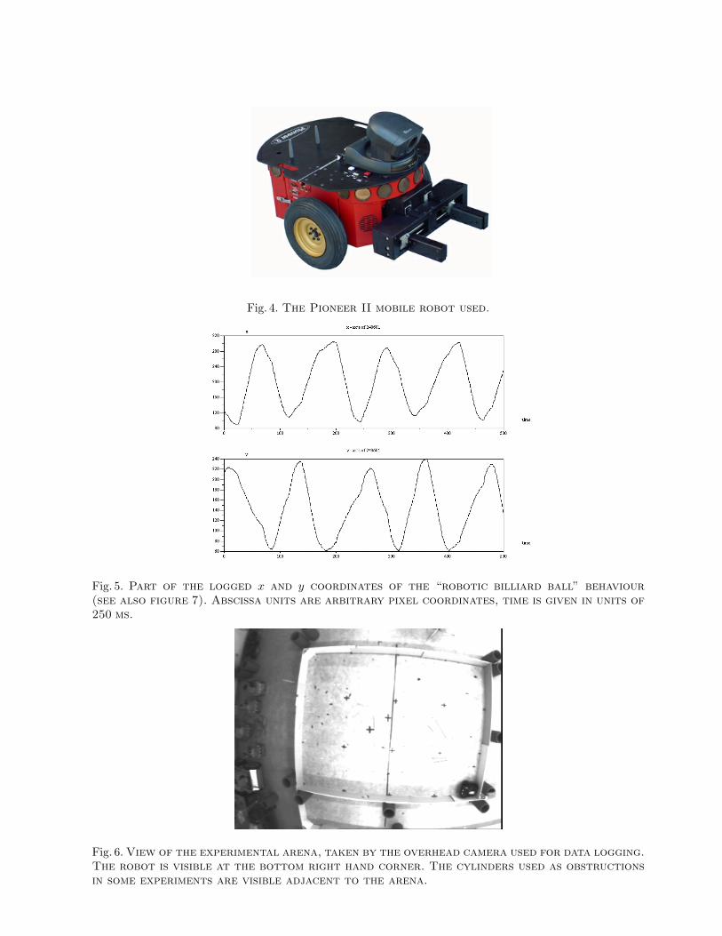
Fig. 4. The Pioneer II mobile robot used.

Fig. 5. Part of the logged x and y coordinates of the “robotic billiard ball” behaviour

(see also figure 7). Abscissa units are arbitrary pixel coordinates, time is given in units of

250 ms.

Fig. 6. View of the experimental arena, taken by the overhead camera used for data logging.

The robot is visible at the bottom right hand corner. The cylinders used as obstructions

in some experiments are visible adjacent to the arena.

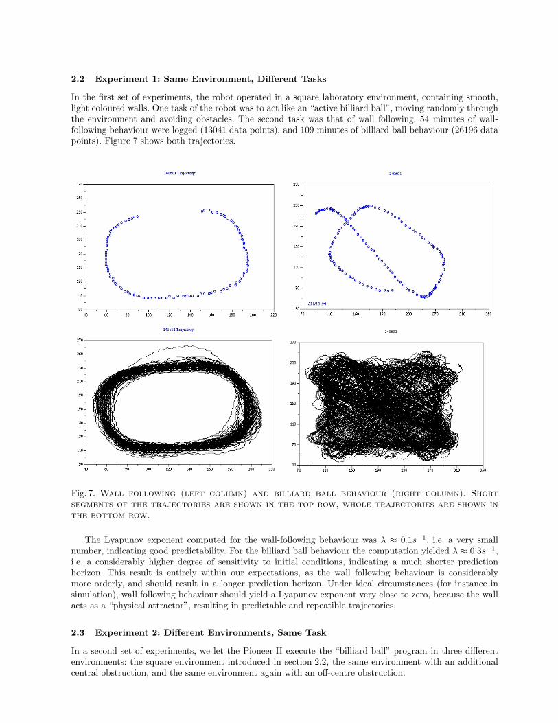
2.2 Experiment 1: Same Environment, Different Tasks

In the first set of experiments, the robot operated in a square laboratory environment, containing smooth,light coloured walls. One task of the robot was to act like an “active billiard ball”, moving randomly throughthe environment and avoiding obstacles. The second task was that of wall following. 54 minutes of wall-following behaviour were logged (13041 data points), and 109 minutes of billiard ball behaviour (26196 datapoints). Figure 7 shows both trajectories.

Fig. 7. Wall following (left column) and billiard ball behaviour (right column). Short

segments of the trajectories are shown in the top row, whole trajectories are shown in

the bottom row.

The Lyapunov exponent computed for the wall-following behaviour was λ ≈ 0.1s−1, i.e. a very smallnumber, indicating good predictability. For the billiard ball behaviour the computation yielded λ ≈ 0.3s−1,i.e. a considerably higher degree of sensitivity to initial conditions, indicating a much shorter predictionhorizon. This result is entirely within our expectations, as the wall following behaviour is considerablymore orderly, and should result in a longer prediction horizon. Under ideal circumstances (for instance insimulation), wall following behaviour should yield a Lyapunov exponent very close to zero, because the wallacts as a “physical attractor”, resulting in predictable and repeatible trajectories.

2.3 Experiment 2: Different Environments, Same Task

In a second set of experiments, we let the Pioneer II execute the “billiard ball” program in three differentenvironments: the square environment introduced in section 2.2, the same environment with an additionalcentral obstruction, and the same environment again with an off-centre obstruction.

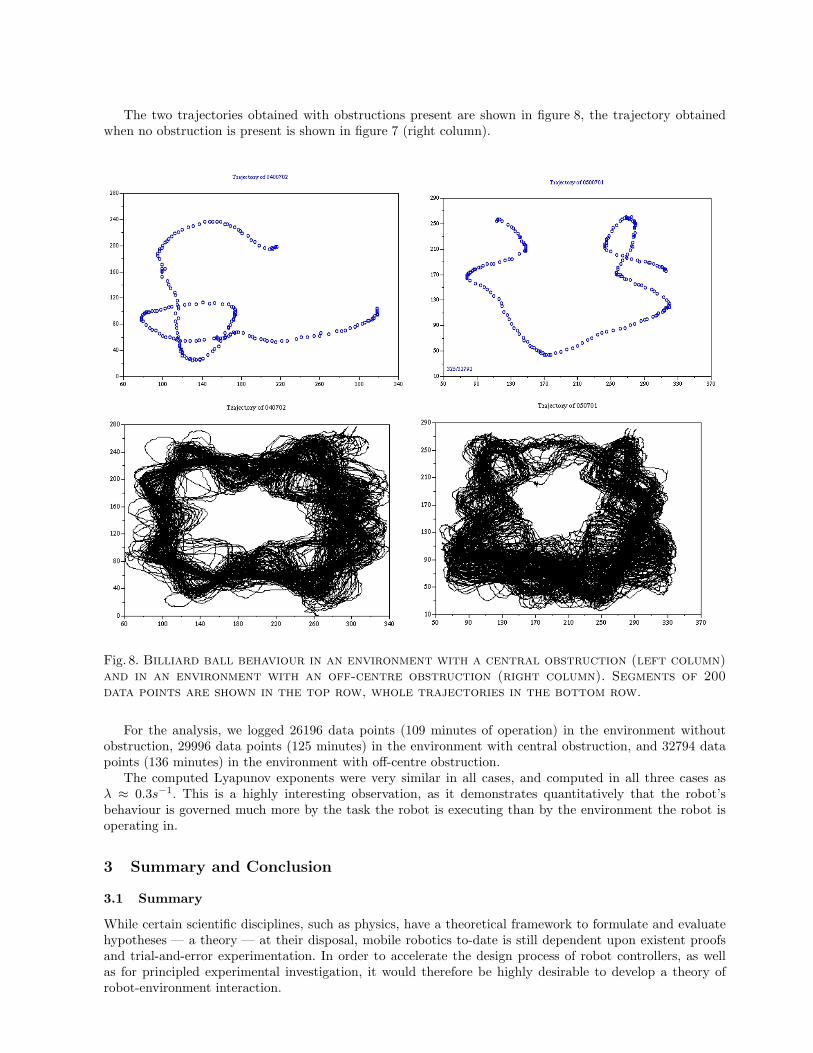
The two trajectories obtained with obstructions present are shown in figure 8, the trajectory obtainedwhen no obstruction is present is shown in figure 7 (right column).

Fig. 8. Billiard ball behaviour in an environment with a central obstruction (left column)

and in an environment with an off-centre obstruction (right column). Segments of 200

data points are shown in the top row, whole trajectories in the bottom row.

For the analysis, we logged 26196 data points (109 minutes of operation) in the environment withoutobstruction, 29996 data points (125 minutes) in the environment with central obstruction, and 32794 datapoints (136 minutes) in the environment with off-centre obstruction.

The computed Lyapunov exponents were very similar in all cases, and computed in all three cases asλ ≈ 0.3s−1. This is a highly interesting observation, as it demonstrates quantitatively that the robot’sbehaviour is governed much more by the task the robot is executing than by the environment the robot isoperating in.

3 Summary and Conclusion

3.1 Summary

While certain scientific disciplines, such as physics, have a theoretical framework to formulate and evaluatehypotheses — a theory — at their disposal, mobile robotics to-date is still dependent upon existent proofsand trial-and-error experimentation. In order to accelerate the design process of robot controllers, as wellas for principled experimental investigation, it would therefore be highly desirable to develop a theory ofrobot-environment interaction.

The foundation of any theory is a quantitative description of experimental results. In this paper, we presentexperiments with an autonomous mobile robot, in which we analyse the robot’s behaviour quantitatively,using concepts from chaos theory.

3.2 Conclusion

Assuming that there are three main aspects that influence the overall behaviour of the robot — robot,task and environment — we conducted two experiments in which two of the three components were keptunchanged, whilst the third component was modified.

In a first set of experiments we let the robot conduct two different tasks in the same environment. Ourfinding was that the Lyapunov exponent differed markedly between the two tasks, signifying that the overallbehaviour of the robot differed between the two experiments, and that this must have been due to thechanged control program (because this was the only changed parameter in our experimentation).

In a second set of experiments we kept robot and task constant, and varied the environment. TheLyapunov exponent was the same in any of the three environments we used, indicating that the overallbehaviour of the robot was not noticeably influenced by the environment the robot was operating in.

While these results require further consolidation, they are nevertheless interesting and encouraging. Theyseem to indicate that robot-environment interaction is far more influenced by the control program — aparameter that the user has influence over — than the environment — a parameter the user often has noinfluence over. This raises hopes that it might eventually be possible to develop a theory that will allow todesign robot control programs without trial-and-error experimentation, and to make predictions regardingthe robot behaviour before an experiment is conducted.

3.3 Future Work

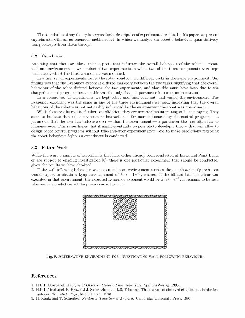
While there are a number of experiments that have either already been conducted at Essex and Point Lomaor are subject to ongoing investigation [6], there is one particular experiment that should be conducted,given the results we have obtained.

If the wall following behaviour was executed in an environment such as the one shown in figure 9, onewould expect to obtain a Lyapunov exponent of λ ≈ 0.1s−1, whereas if the billiard ball behaviour wasexecuted in that environment, the expected Lyapunov exponent would be λ ≈ 0.3s−1. It remains to be seenwhether this prediction will be proven correct or not.

Fig. 9. Alternative environment for investigating wall-following behaviour.

References

1. H.D.I. Abarbanel. Analysis of Observed Chaotic Data. New York: Springer-Verlag, 1996.2. H.D.I. Abarbanel, R. Brown, J.J. Sidorowich, and L.S. Tsimring. The analysis of observed chaotic data in physical

systems. Rev. Mod. Phys., 65:1331–1392, 1993.3. H. Kantz and T. Schreiber. Nonlinear Time Series Analysis. Cambridge University Press, 1997.

4. H. Kantz and T. Schreiber. TISEAN — Nonlinear Time Series Analysis. URL=http://www.mpipks-dresden.mpg.de/ tisean/, Last access May 2003.

5. D. Kaplan and L. Glass. Understanding Nonlinear Dynamics. Springer Verlag London, 1995.6. U. Nehmzow and K. Walker. Is the behaviour of a mobile robot chaotic? In Proc. AISB Convention Aberystwyth,

ISBN 1 902956 32 3, 2003.7. H.-O. Peitgen, H. Jurgens, and D. Saupe. Chaos and Fractals. Springer Verlag, 1992.8. Applied Nonlinear Sciences. Tools for Dynamics. http://www.zweb.com/apnonlin, Last access May 2003.9. A Wolf, J. Swift, H. Swinney, and J. Vastano. Determining lyapunov exponents from a time series. Physica 16D,

1995.