Quantitative Assessment of Quantitative Assessment of Human Bone Tissue by Novel Human Bone Tissue by Novel

Ultrasound TechniquesUltrasound Techniques

Presenter : Pei - Jarn ChenPresenter : Pei - Jarn Chen

NCKU BME Ultrasound Lab.

OutlineOutline1. Introduction1. Introduction ---- Osteoporosis---- Osteoporosis ---- Quantitative Ultrasound (QUS)---- Quantitative Ultrasound (QUS)2. Motivations2. Motivations3. Material and Methods3. Material and Methods (a) Quantitative assessment of osteoporosis from (a) Quantitative assessment of osteoporosis from

the tibia shaft by the tibia shaft by dual-transducers techniquedual-transducers technique (b) Measurements of ultrasonic parameters on (b) Measurements of ultrasonic parameters on

calcaneus by calcaneus by two-sided interrogation two-sided interrogation techniquestechniques

(c) Measurements of acoustic velocity dispersion (c) Measurements of acoustic velocity dispersion on calcaneus using on calcaneus using time-domain split spectrum time-domain split spectrum processing (SSP) techniquesprocessing (SSP) techniques

4. Results4. Results5. Conclusion and Discussion5. Conclusion and Discussion6. Future developments6. Future developments

IntroductionIntroduction1. Osteoporosis1. Osteoporosis

http://www.mayohealth.com http://www.nof.org

WHO : (1994)Osteoporosis is defined as a disease characterized by both a loss of bone mass and microarchitecture alteration, leading to hyperfragility, and to an uncommonly high risk of fracture.

cortical

cancellous (trabecular)

Type I : -- induced by estrogen

deficiency -- women after menopause

Type II : -- Senile osteoporosis-- affects both sexes after age

70 and results in a reduced bone density of both the cortical and trabecular bone

http://www.mayohealth.com/

http://medlib.med.utah.edu/ http://www.jococ.org/

2. 2. Bone Density Assessment System Bone Density Assessment System in Clinicin Clinic

(a) Non-ultrasound techniques SPA (Single Gamma Photon

Absorptiometry) DPA (Dual Gamma Photon

Absorptiometry) DEXA (Dual-Energy X-ray

Absorptiometry) QCT (X-ray Computed Tomography)

----- BMD (Bone Mineral Density, g/cm2, g/cm3)

Disadvantages : (1) radiation (2) high cost (3) mechanical properties ?

(b) Ultrasound techniques ---- QUS (quantitative ultrasound) Advantages: (1) moveable (2) radiation free (3)

low cost

DEXA----- Lunar DPX

RegionRegion AreaArea BMC(g)BMC(g) BMD(g/cmBMD(g/cm22)) T-scoreT-score Z-scoreZ-score

NeckNeck 4.704.70 3.983.98 0.8470.847 -0.0-0.0 0.30.3

TrochTroch 8.288.28 6.956.95 0.8390.839 1.31.3 1.51.5

InterInter 15.7615.76 19.1319.13 1.2141.214 0.70.7 0.80.8

TotalTotal 28.7428.74 1.051.05 0.8090.809 0.60.6 1.31.3

Normal T-score > -1Low bone mass -2.5 < T-score < -1Osteoporosis T< -2.5Severe osteoporosis (1) T < -2.5 (2) fracture* Unit : SD (standard deviation)

WHO criteria

• T- score: the difference in SD between the individual’s BMD and the mean BMD of health young (24-40).• Z - score: bone density compared with that of an average of people in same age group and gender

Broadband Ultrasound Attenuation ( BUA )

Speed of Sound ( SOS ) E: Young’s Modulus : density

Acoustic impedance Backscattering coefficient

(AIB, apparent integrated backscattering) Velocity dispersion

E

v

xfeII )(0

cz

3. Quantitative Ultrasound (QUS)3. Quantitative Ultrasound (QUS)

water

bone

BUA BUA (dB / MHz)(dB / MHz) Measurement Measurement

Signal Frequency domain

fyxBUA

fyxA

fyxAfyx

MHzslope

r

,,

,,

,,*20,,

]6.02.0[

log

BUABUA

f

dB

FFT

)(

)(

21

21

ttt

ssx

t

xvelocityBone

xb

b

xtx

velocityLimb

SOS measurements

(1) Time domain (signal velocity, group velocity)

* TOF : time of flight

Time of Flight ( TOF)

1. First Arrival2. Threshold3. Zero Crossing4. Envelope Peak

T

1234

P. H. F. Nicholson, G. Lowet, C. M. Langton, J. Dequeker and G. Van der Perre, “ A comparison of time-domain and frequency-domain approaches to ultrasonic velocity measurement in trabecular bone”, Phys. Med.Biol., 41, pp. 2421-2435, 1996.

water

bone

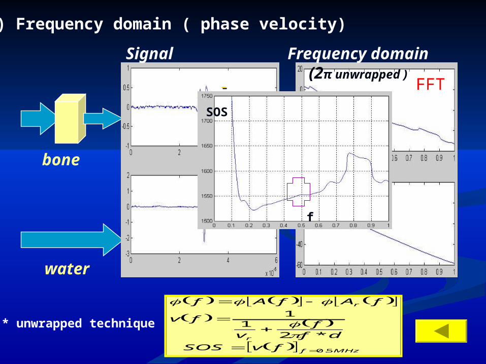
Signal Frequency domain (2π unwrapped )

MHzf

r

r

fvSOS

dff

v

fv

fAfAf

5.0

*21

1

(2) Frequency domain ( phase velocity)

* unwrapped technique

f

SOS

FFT

◆ ◆ based on : attenuated with power lawbased on : attenuated with power law

dss

s

VV PP

0

20

)(2

)(

1

)(

1

Velocity Dispersion

yii 0

※ Kramers – Kronig Relationship ( O’Donnell , 1981)( O’Donnell , 1981)

※ Conventional approaches (a) time domain (b) frequency domain

VDM may convey important structural information not already contained in BMD, SOS, or BUA . ( Droin, 1998)

＊ ＊ Velocity dispersion Velocity dispersion magnitudemagnitude ( m s( m s-1-1 MHz MHz-1-1)) VDM = ∆V = V( fmax ) - VDM = ∆V = V( fmax ) - V( fmin )V( fmin )

Conventional velocity dispersion measurements

frequency domain

fdfC

CfV

w

wp )(

1)(

Vp(f) : phase velocity

Cw : acoustic speed in water

d : thickness of phantom

f : frequency

(f) : phase difference

between water and medium

time domain

f1f2

fn

f1

f2

fn

Vp(f1)me

diu

m

Vp(f2)

Vp(fn)

1. discontinuity

2. absolute phase

* substitution method

Recent VDM researches on Recent VDM researches on Calcaneus Calcaneus in vitroin vitro measurements measurements

Authors n Frequency range Dispersion (mean ± standard (kHz) deviation) (m s-1 MHz-1)

Wear (2000)

Nicholson et al (1996)

Strelitizki and Evans (1996)

Dorin et al (1998)

24 200-600 -18 ± 15

70 200-800 -40

10 600-800 -32 ± 27

15 200-600 -15 ± 13

Negative (63/70)

Positive (7/70)

P. H. F. Nicholson, G. Lowet, C. M. Langton, J. Dequeker and G. Van der Perre, “ A comparison of time-domain and frequency-domain approaches to ultrasonic velocity measurement in trabecular bone”, Phys. Med. Biol., 41, pp. 2421-2435, 1996.

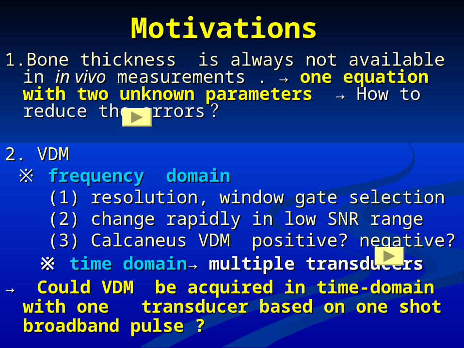
Motivations Motivations 1.Bone thickness is always not available in 1.Bone thickness is always not available in in in

vivovivo measurements . measurements . → → one equation with one equation with two unknown parameterstwo unknown parameters → How to reduce → How to reduce the errorsthe errors ？？

2. VDM2. VDM ※ ※ frequency frequency domaindomain (1) resolution, window gate selection(1) resolution, window gate selection (2) change rapidly in low SNR range(2) change rapidly in low SNR range (3) Calcaneus VDM positive? negative?(3) Calcaneus VDM positive? negative? ※ ※ time domaintime domain→ multiple transducers→ multiple transducers→ → CouldCould VDM be acquired in time-domain VDM be acquired in time-domain

with one transducer based on one shot with one transducer based on one shot broadband pulse ?broadband pulse ?

(a) Contact (dry) type

(b) Water bath

Achilles Lunar

CUBA QUS-2 SoundScan 2000DBM 2000

wbone

bonew

Vd

dVV

w

p

bone

p

p

V

dd

d

V

VV

1

1

15 20 25 30 35 40 45 50-40

-30

-20

-10

0

10

20

30

40

true calcaneus width (mm)

err

or

(%)

SOS: 1600 m/sSOS: 2000 m/sSOS: 3000 m/s

The SOS estimation errors vs. true bone tissue thickness for different bone velocities assuming a preset bone thickness of 40 mm. ( ＋ : 1600 m/s, ＊ : 2000 m/s, : 3000 m/s).◇

1. For a dry system, a 6 mm decrease in heel thickness caused an increase of 24 m/s in SOS as reported by Johansen

2. For a dry system, such as CUBA system, presses transducers against the skin to obtain the calcaneus width and the mean speed of sound (SOS) measured by contact type (soft tissue intact) is lower 89 m/s than the mean bone SOS (no soft tissue) in in vitro measurements .

1. A. Johansen, and M. D. Stone, “ The effect of angle edema on bone ultrasound assessment of the heel,” Osteoporos Int., vol. 7, pp. 44-47, 1997.

2. K. D. Häulser, etc. “ Water bath and contact methods in ultrasonic evaluation of bone,” Calcif Tissue Int., vol. 61, pp. 26-29, 1997.

Material and Methods

1.1. Quantitative assessment of osteoporosisQuantitative assessment of osteoporosis from the tibia shaft by from the tibia shaft by dual-ultrasound dual-ultrasound

techniquetechnique

3. Measurements of acoustic velocity 3. Measurements of acoustic velocity dispersion on calcaneus using dispersion on calcaneus using time-time-domain split spectrum processing (SSP) domain split spectrum processing (SSP) techniquetechnique

2.2. Measurements of ultrasonic parameters onMeasurements of ultrasonic parameters on calcaneus by calcaneus by two-sided interrogation two-sided interrogation

techniquetechnique

1

2

xCw

1

2 2xC

zCw b

2 x

CBECw w

2

xC

zC

CDC

DECw b b w

A--B--A

A--B--C--B--A

A--B--E

A--B--C--D--E

--------------(1)

---------------(2)

---------------------------(3)

---------(4)

#1

#2 x z

A B

D

CTransducer

Transducer

y

E

Coupling medium Tibia shaft

Dual-ultrasound Dual-ultrasound techniquetechnique

b

w

C

Czz : Effective distance

z

(transmitter & receiver)

( receiver)

,1 1

,2 2

Cb

Cy

K Kb

( )

[( ) ] ( )

1

1 2 1 2

111 2 2 2

K

1

212

2 2 1

12 2

1

4 2( )

( )and

: the TOFs from the trigger of the transmitting pulse to the front and the rear echoes of bone tissue received by transducer #1

: the TOFs on transducer #2

: sound speed in bone tissue (tibia)

y : the separation distance of two transducers

then

where

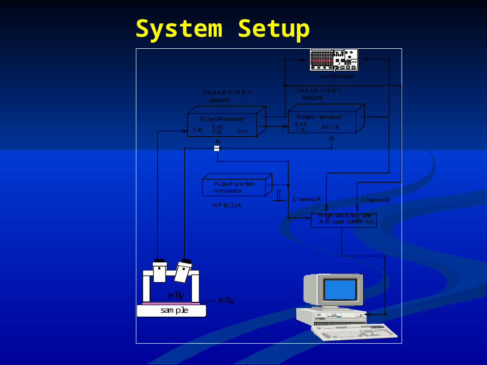
Pulser/Receiver

PANAMETRICS

5058PR

PANAMETRICS

5052PR

High sampling rateA/D card (100Mhz)

Channel A Channel B

T/R RCVR

Pulse/FunctionGenerator

Pulser / receiver

Ext.Tri.

Ext.Tri.Syn.

oscilloscope

HP 8111A

Jelly

sampleJelly

System Setup

Theoretical DerivationTheoretical Derivation

w

ww V

dt

dw

ffmw

bf

ff tV

dddd

V

d

V

ddm

)( 2121

)(f

fwdwfm

mwb

V

dttVdd

dVV

Vf = 1540 m/s

Vw= 1487 m/s at 22 oC

Two-sided interrogation Two-sided interrogation techniques (1)techniques (1)

* df = df1= df2

2121 tt

V

d

f

f

2342 tt

V

d

f

f

dw

ffmw

bf

ff tV

dddd

V

d

V

ddm

)( 2121

)22

()22

( 341231 ttttV

ttVdd fwwm

)2

()(2

34123412

ttttttVtttt

Vd

dVV

wdwf

m

mwb

Two-sided interrogation Two-sided interrogation techniques (2)techniques (2)

System ArchitectureSystem Architecture

TransducerTransducerTransducer: Part number : Panametrics V391Frequency : 0.5 MHzType : Immersion transducerElement size : 29 mm (1.125")Focusing configurations :1.5", PTF (Point Target Focus) Spherical focus

1. Good axial resolution

2. Improved signal-to-noise (SNR) in attenuated or scattering materials

x1

x2

xn

x1’

x2’

xn’

med

ium

Velocity dispersion ?

f ( Hz )

V (m/s)

A0(t) A(t)

decompose decompose

VDM ----- Theory development

※ ※ SSP - SSP - Bilgutay, 1981 Bilgutay, 1981

BPF : bandpass filter

Split Spectrum Processing (SSP)

Y(t)

BPF f1(t)

BPF f2(t)

BPF fn(t)

X’1(t)

X’2(t)

X’n(t)

Y’(t)

expansion reconstruction

filter bank

x’n(t)

N

i

N

iii tythty

1 1

)()()(

)()()( fYfHfY

n

ii fHfH

1

)()(

)2sin()(2

2

2 tfAeth i

t

it

if H(f) =1

Bandpass filter bank design

5

2000 5 10

0 2000 4000 6000 0 5 10 15

x 105

each gaussion filter in t domain FFT of each Gaussion filter

Hz

x

fB ci

2

Total filter numbers

N = BT + 1B: total bandpass filter width ( fmax- fmin )

T : total signal time

fc: central frequency

: predetermined threshold

: attenuation coefficient

X: thickness

Each filter bandwidth

Bi = 50 kHz

( Ping He, 1998 )

( Karpur, 1987 )

0 2 4 6 8 10 12

x 105

0

0.2

0.4

0.6

0.8

1

1.2

1.4

Hz

Summed bandpass filter

Individual Gaussian filter

fmin fmax

B

1,....,0minmaxmin

Nnn

N

ffffi

t f

1 2 3 4 5 6 7 8 9 10

x 104

10-7

10-6

10-5

10-4

10-3

The ROC curve of gauss filter width with RMS error

RM

S e

rror m

agni

tude

gaussion band width (Hz)

-150 m/s-40m/s 0 m/s 40 m/s 150 m/s

1 2 3 4 5 6 7 8 9 10

x 104

-2000

-1500

-1000

-500

0

500

1000 The ROC curve of gaussion filter width with velocity error

gaussion band width (Hz)

velo

city e

rror

(m/s

)

-150 m/s-40 m/s 0 m/s40 m/s 150 m/s

Gaussian Filter Design

NiyixEN

irms /)()(

2

1

＊ optimal bandwidth

→ 50 KHz

Reconstruction error Error between preset velocity and SOS evaluated

0 1000 2000 3000 4000 5000 6000-1

-0.8

-0.6

-0.4

-0.2

0

0.2

0.4

0.6

0.8

1

b--- input signal with SSPk--- simulated input signal

Velocity dispersion and BUA estimation

0 2000 4000 6000 0 2000 4000 6000

BUAi

incident transmission

)(

)(log20

tA

tABUA

ri

ii

d : medium thickness

ti : time of difference

Cw : acoustic speed in water

phase velocity

d

tCC

fViw

wip

1)(

Ai(t) : narrow band incident signal in time domain

Ari(t) : narrow band reference signal through water

Δti

ResultsResults

1.1. Quantitative assessment of osteoporosisQuantitative assessment of osteoporosis from the tibia shaft by from the tibia shaft by dual-ultrasound dual-ultrasound

techniquetechnique

3. Measurements of acoustic velocity 3. Measurements of acoustic velocity dispersion on calcaneus using dispersion on calcaneus using time-time-domain split spectrum processing (SSP) domain split spectrum processing (SSP) techniquetechnique

2.2. Measurements of ultrasonic parameters onMeasurements of ultrasonic parameters on calcaneus by calcaneus by two-sided interrogation techniquetwo-sided interrogation technique

thi cknes

s

(mm)

1

(sec)

1

(sec)

2

(sec)

2

(sec)

sos

(m/ sec)

y

(mm)

8.96 62.80 69.32 63.28 70.84 2748.5 8.5720

Thickness= 8.96 mm, SOS= 2748.5 m s-1 Plexiglas

System performance test (1)

τ1τ1

τ2 τ2’

τ1’

0 20 40 60 80 100 120-1.5

-1

-0.5

0

0.5

1

0 20 40 60 80 100 120-1

-0.5

0

0.5

1

Dual-ultrasound techniquesDual-ultrasound techniques

0 20 40 60 80 100 120-1.5

-1

-0.5

0

0.5

1

0 20 40 60 80 100 120-1

-0.5

0

0.5

1

thi ckness

(mm)

y

(mm)

1

(sec)

1

(sec)

2

(sec)

2

(sec)

SOS*2

(m/ sec)

* 8.5720 65.64 70.16 65.74 71.02 2731.3

unknown thickness Plexiglas

System performance test (2)

Accuracy = 99.3%

CV%= 3.53 % for 10 measurementsat different sites

In-vivo measurements

0 20 40 60 80 100 120 140 160 180-1

-0.8

-0.6

-0.4

-0.2

0

0.2

0.4

0.6

0.8

1

0 50 100 150 200 250 300-0.2

-0.15

-0.1

-0.05

0

0.05

0.1

0.15

0.2

0 20 40 60 80 100 120-4

-2

0

2

4

0 20 40 60 80 100 120-2

-1

0

1

2

0 20 40 60 80 100 120-1

-0.5

0

0.5

1

1.5

0 20 40 60 80 100 120-1.5

-1

-0.5

0

0.5

1

normal subject

osteoporosis

0 .90 1 .00 1 .10 1 .20 1 .30

B M D (g/ cm ^2)

2500 .00

3000 .00

3500 .00

4000 .00

4500 .00

SO

S (m

/s)

Subjects: --- 18 outpatients recruited from NCKU Hospital--- suffering from low back pain, radiological evidence of

osteoporosis and/or compression fracture of the vertebral body -- post-menopausal or senile osteoporosis: 5 males, 4 females

( mean age 65 years, 56 ~ 73 )-- nine patients had been immobilized for more than 3 months

after various orthopedic surgeries ( mean age 52 years, 21 ~ 72)

R= 0.93

BMD- measured by DEXA (Lunar DPX, radiology of NCKU Hospital)

Two-sided interrogation techniquesTwo-sided interrogation techniques

In vitro measurements

model 2583model 2572

2583: normal bone SOS = 1576 m s-1 BUA= 69 dB/MHz 2572: osteoporosis SOS = 1501 m s-1 BUA= 48 dB/MHz

porcine skin (7.3 mm)

Set df1=df2 =0, t1= t2, t3= t4

porcine skin thickness = 7.3 mm

(~ 43.6 mm)

In vivoIn vivo measurements measurements

Subjects : 6 males 8 females Measurement site : left calcaneus

Echo Signals : Subject No.1, Male, Age 24

Echo Signals : Subject No.2, Female, Age Echo Signals : Subject No.2, Female, Age 2323

Transmission SignalsTransmission Signals

In vivoIn vivo measurements measurements

Time-domain split spectrum processing Time-domain split spectrum processing (SSP) techniques(SSP) techniques

※ Model-based ultrasound signals with velocity dispersion

FN(fN)

RN(t)

R(t)

Y(t)

R2(t)

R1(t)

f1 f2 fN

f1 f2 fN

f1 f2 fN

F1(f1)

F2(f2)

attenuation & dispersion

Fig. Schematic representation of model-based ultrasound signal

0022 22/)( ifit eeAetY t Σ

Ri(t) Time delay tgi Zi(t)dfie

)( 0ffbC

dt

issogi

)()( tZtZ i

2600 2800 3000 3200 3400 3600 3800

-0.1

-0.05

0

0.05

0.1

-150 m/s MHz-80 m/s MHz -40 m/s MHz 0 m/s MHz

2600 2800 3000 3200 3400 3600 3800

-0.1

-0.05

0

0.05

0.1

0 m/s MHz 40 m/s MHz 80 m/s MHz 150 m/s MHz

0 1000 2000 3000 4000 5000 6000-1

-0.8

-0.6

-0.4

-0.2

0

0.2

0.4

0.6

0.8

1k- simulated input signalr-- simulated output signal

bs= - 80 m/s MHzcalcaneus: 2 cmattenuation : 20 dB1550 m/s at 0.5 MHz

bs : velocity dispersion parameters (m/s MHz)Cso : group velocityf0 : central frequency

The simulation results of an ultrasound pulse transmits the calcaneus with velocity dispersion ( -80 m s-1 MHz-1)

negative dispersion

positive dispersion

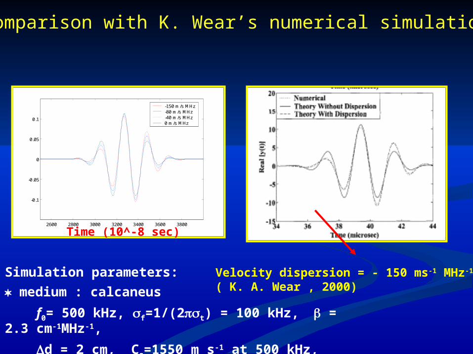
※ Comparison with K. Wear’s numerical simulation

Simulation parameters: medium : calcaneus

f0= 500 kHz, f=1/(2t) = 100 kHz, = 2.3 cm-1MHz-1,

d = 2 cm, Cs=1550 m s-1 at 500 kHz, 0=0, Cw=1480 m s-1

2600 2800 3000 3200 3400 3600 3800

-0.1

-0.05

0

0.05

0.1

-150 m/s MHz-80 m/s MHz -40 m/s MHz 0 m/s MHz

Velocity dispersion = - 150 ms-1 MHz-1

( K. A. Wear , 2000)

Time (10^-8 sec)

2 3 4 5 6 7 8 9

x 105

1450

1500

1550

1600

1650

Hz

SOS

(m/s

)

bs = -150 m/sMHz

bs = 150 m/sMHz

Fig. The analysis of phase velocity by SSP technique with various velocity dispersion. ( -150 m s-1 MHz-1 ~ 150 m s-1 MHz-1) - : preset value + : SOS predicted by SSP technique

SSP results with model-based ultrasound signals

Preset VDM (m/s Preset VDM (m/s MHz)MHz)

Predicted VDM by Predicted VDM by SSPSSP

Error Error (%)(%)

150150 126.52126.52 15.6615.66

8080 72.6272.62 9.229.22

4040 36.6536.65 8.378.37

00 0.00.0 0.00.0

-40-40 -36.68-36.68 8.308.30

-80-80 -72.59-72.59 9.269.26

-150-150 -125.96-125.96 16.0216.02

※ The comparisons with conventional The comparisons with conventional techniques in frequency-domaintechniques in frequency-domain

Conventional techniqueConventional technique ( Nicholson, 1996)( Nicholson, 1996)

2π unwrapped

Circular- rotating Circular- rotating technique (Ping He, technique (Ping He, 2001)2001)

2 3 4 5 6 7 8 9 10 11 12

x 105

1000

1100

1200

1300

1400

1500

1600

1700

1800

1900

2000

Hz

SO

S (

m/s

)

VDM by SSPPreset VDMVDM by f-domainVDM by Ping He

Bs= -40 m/s

2 3 4 5 6 7 8 9 10 11 12

x 105

1000

1100

1200

1300

1400

1500

1600

1700

1800

1900

2000

Hz

SOS (

m/s)

VDM by SSPPreset VDMVDM by f-domainVDM by Ping He

Bs= 0 m/s MHz

2 3 4 5 6 7 8 9 10 11 12

x 105

1000

1100

1200

1300

1400

1500

1600

1700

1800

1900

2000

Hz

SO

S (

m/s

)

VDM by SSPPreset VDMVDM by f-domainVDM by Ping He

Bs= 40 m/s

Bs= - 40 m/s MHz

Bs= 40 m/s MHz

Bs= 0 m/s MHz

mimic calcaneus phantoms mimic calcaneus phantoms a. a. normal bonenormal bone (model 2583, CIRS Inc., Norfolk, VA. )(model 2583, CIRS Inc., Norfolk, VA. ) manufacturer’s specifications manufacturer’s specifications ::

thickness 3.63 cm, SOS = 1576 m sthickness 3.63 cm, SOS = 1576 m s -1-1, ,

BUA= 69 dB MHzBUA= 69 dB MHz-1-1 ( 0.2 ~ 0.55 MHz ) ( 0.2 ~ 0.55 MHz )

b. b. osteoporosis boneosteoporosis bone

(model 2572, CIRS Inc., Norfolk, VA. )(model 2572, CIRS Inc., Norfolk, VA. ) manufacturer’s specifications : manufacturer’s specifications :

thickness 3.64cm, SOS = 1510 m sthickness 3.64cm, SOS = 1510 m s -1-1, ,

BUA= 48 dB MHzBUA= 48 dB MHz-1-1 ( 0.2 ~ 0.55 MHz) ( 0.2 ~ 0.55 MHz)

Phantoms measurements

model 2583 model 2572* SOS: speed of sound

0.5 MHz unfocused0.5 MHz unfocused

2 * Transducer 2 * Transducer

T/R : 5058 PR, Panametrics Inc., Waltham, MA.

oscilloscope: TDS 520D, ( Tektronix Inc., Beaverton, OR.)

Measurement system

0 .00 200000 .00 400000 .00 600000 .00 800000 .00 1000000 .00

1450 .00

1500 .00

1550 .00

1600 .00

1650 .00

1700 .00

SO S (m / s)

H z

Phantom VDM by SSP(mean ± SD)(m / s MHz)

Signal velocity

(manufacturer’s specifications )(m / s)

Signal velocity by SSP(μ ± σ m/s)(m / s)

normal 1 85.41 ± 9.63 1576 1559.72 ± 7.51

osteoporosis 2 34.08 ± 4.15 1510 1499.98 ± 2.37

Fig. The comparisons of signal velocity(: 0.25, 0.5, 0.75 MHz) and phase velocity analyzed by SSP technique [ osteoporotic bone phantom ( ＊ ), normal bone phantom ()].

1. normal bone: CIRS ( model: 2583)2. osteoporotic bone: CIRS ( model : 2572)

0 1 2 3 4 5 6 7 8 9 10

x 105

1200

1300

1400

1500

1600

1700

1800

Hz

phas

e ve

locity

(m/s

)

group velocityphase velocity by SSPphase velocity (unwrap)phase velocity (cir. rot.)

0 1 2 3 4 5 6 7 8 9 10

x 105

1200

1300

1400

1500

1600

1700

1800

Hz

phas

e ve

locity

(m/s

)

group velocityphase velocity by SSPphase velocity (unwrap)phase velocity (cir. rot.)

The comparisons between time-domain The comparisons between time-domain SSP and conventional techniques in SSP and conventional techniques in frequency-domainfrequency-domain

Normal bone phantom (Model 2583) ※ different window gate selection

0 1 2 3 4 5 6 7 8 9 10

x 105

1200

1300

1400

1500

1600

1700

1800

Hz

phas

e ve

loci

ty (m

/s)

group velocityphase velocity by SSPphase velocity (unwrap)phase velocity (cir. rot.)

0 1 2 3 4 5 6 7 8 9 10

x 105

1200

1300

1400

1500

1600

1700

1800

Hz

phas

e ve

locity

(m/s

)

group velocityphase velocity by SSPphase velocity (unwrap)phase velocity (cir. rot.)

The comparisons between time-domain The comparisons between time-domain SSP and conventional techniques in SSP and conventional techniques in frequency-domainfrequency-domain

Osteoporosis phantom (Model 2572) ※ different window gate selection

In vivo measurements

Sampling rate 50 MHzCentral frequency 0.7 MHzHeel width 45 mm(1) subject_1

(2) subject_4

Sampling rate 50 MHzCentral frequency 0.7 MHzHeel width 53 mm

VP : group velocity by envelop peak Vc : group velocity at 0. 8 MHz by SSP techniqueVDM : velocity dispersion magnitude between 0.4 ~ 1.2 MHz

SOSUBIS: SOS by UBIS 5000BUAUBIS: BUA by UBIS 5000

The results of in vivo measurements on calcaneus

Discussion (1)Discussion (1)(a) Quantitative assessment of osteoporosis from the (a) Quantitative assessment of osteoporosis from the

tibia shaft by tibia shaft by dual-ultrasound techniquedual-ultrasound technique

1. Without knowing he thickness of tibia, the proposed 1. Without knowing he thickness of tibia, the proposed techniques can estimate the SOS with tibia, only from techniques can estimate the SOS with tibia, only from the different TOFs acquired from two transducers.the different TOFs acquired from two transducers.

2. High accuracy ( 99 %) and low CV (3.53 %) reveal in 2. High accuracy ( 99 %) and low CV (3.53 %) reveal in Plexiglas phantom measurements with developed Plexiglas phantom measurements with developed system.system.

3. High correlation coefficient (R = 0.93) exists between 3. High correlation coefficient (R = 0.93) exists between BMD (DEXA) and SOS BMD (DEXA) and SOS in vivoin vivo measurements. measurements.

Discussion (2-1)Discussion (2-1)(b) Measurements of ultrasonic parameters on(b) Measurements of ultrasonic parameters on

calcaneus by calcaneus by two-sided interrogation techniquetwo-sided interrogation technique1. The proposed two-sided interrogation technique can 1. The proposed two-sided interrogation technique can

directly measure the bone thickness and estimates the directly measure the bone thickness and estimates the SOS on calcaneus, neglecting the soft tissue effect.SOS on calcaneus, neglecting the soft tissue effect.

2. Based on the test of bone phantom attached with 2. Based on the test of bone phantom attached with porcine skin , the accuracy with SOS estimation is high porcine skin , the accuracy with SOS estimation is high up 99 % and 96 % using proposed techniquesup 99 % and 96 % using proposed techniques..

3.3. Based on 14 normal subjects Based on 14 normal subjects in vivo in vivo measurements, measurements, the thickness of calcaneus ranged between the thickness of calcaneus ranged between 3.3 ~ 4.7 3.3 ~ 4.7 cmcm and the SOS of calcaneus ranged from and the SOS of calcaneus ranged from 1473 m s1473 m s-1-1 to to 15371537 m sm s-1-1. Those agree with literatures’ reports. . Those agree with literatures’ reports. (1. (1. Glüer, 1995; 29.0 ± 2.9 mm from radiographics, 30.0 ± 2.8 Glüer, 1995; 29.0 ± 2.9 mm from radiographics, 30.0 ± 2.8 mm from CT. 2. Laugier, 1997; 1485 ~ 1550 m smm from CT. 2. Laugier, 1997; 1485 ~ 1550 m s-1-1, 5.8 ~ 18.2 , 5.8 ~ 18.2 dB cmdB cm-1-1 MHz MHz-1-1))

Discussion (2-2)Discussion (2-2)

4. The SOS on calcaneus measured with 4. The SOS on calcaneus measured with proposed technique were lower than the proposed technique were lower than the results with constant accumulated thickness results with constant accumulated thickness (bone + soft tissue) assumption and those (bone + soft tissue) assumption and those from UBIS 5000 measurements.from UBIS 5000 measurements.

Discussion (3-1)Discussion (3-1)(c) Measurements of acoustic velocity (c) Measurements of acoustic velocity

dispersion on calcaneus using dispersion on calcaneus using time-domain time-domain split spectrum processing (SSP) techniquesplit spectrum processing (SSP) technique

1.The SSP technique decomposes a 1.The SSP technique decomposes a

broadband pulse into serial signals having broadband pulse into serial signals having

different frequency using an optimal different frequency using an optimal

bandpass filter bank combined by many bandpass filter bank combined by many

narrow bandpass filter with constant narrow bandpass filter with constant

bandwidth .bandwidth .

2. 2. The VDM can be obtained only from one The VDM can be obtained only from one

shot broadband ultrasound pulse with a shot broadband ultrasound pulse with a

single interrogation.single interrogation.

3. The VDM evaluated by SSP technique are 3. The VDM evaluated by SSP technique are consistent with the simulation on model-consistent with the simulation on model-based signals, especial for the low based signals, especial for the low velocity dispersion ( < 80 m svelocity dispersion ( < 80 m s-1-1 MHz MHz-1-1).).

4. 4. The VDM measurements of two The VDM measurements of two commercial bone phantoms are agreeable commercial bone phantoms are agreeable to the results measured by three to the results measured by three transducers with different central transducers with different central frequencies.frequencies.

Discussion (3-2)Discussion (3-2)

ConclusionConclusion1. Three novel ultrasound techniques 1. Three novel ultrasound techniques

proposed in this thesis are fair simple, proposed in this thesis are fair simple, straightforward and easily performed in straightforward and easily performed in time-domain to estimate the SOS, VDM time-domain to estimate the SOS, VDM on bone tissue.on bone tissue.

2. 2. Based on the phantoms measurements, Based on the phantoms measurements, the simulation with model-based signals the simulation with model-based signals and the and the in vivo in vivo measurements, measurements, respectively; the results reveal that the respectively; the results reveal that the proposed three novel ultrasound proposed three novel ultrasound techniques may have the potential on techniques may have the potential on clinical applications for osteoporosis clinical applications for osteoporosis assessments.assessments.

Future DevelopmentsFuture Developments1. A QUS scan system developed on PC based 1. A QUS scan system developed on PC based

on two-sided interrogation technique has on two-sided interrogation technique has been developed and is in progress . been developed and is in progress .

2. The VDM image based on proposed SSP 2. The VDM image based on proposed SSP technique may be developed in above technique may be developed in above system.system.

3. The techniques proposed in this thesis 3. The techniques proposed in this thesis hope to be performed in an embedded hope to be performed in an embedded SOPC system (System on Programmable SOPC system (System on Programmable Chip) (i.e. FPGA-NIOS system).Chip) (i.e. FPGA-NIOS system).

4. The relations between VDM,4. The relations between VDM, BMD and BMD and bone microstructurebone microstructure are worth to further are worth to further studystudy..

Thanks for your attention !!

Dual Energy X-ray Absorptiometry (DEXA)

SB70B38

o3838o7070SB

BS70S38

o3838o7070BS

R

)/I(Iln)/Iln(IRM

R

)/I(Iln)/Iln(IRM

R

RS S38 S70

B B38 B70

where:

I I exp[-( M M )]

I I exp[- M M )]38 o38 S38 S B38 B

70 o70 S70 S B70 B

(

Imaging ultrasound Imaging ultrasound densitometry:densitometry: UBIS 5000(DMS) UBIS 5000(DMS)

Reference CurveReference Curve

407 healthy Caucasian U.S. females,ranging in age from 20 to 79 years were used to establish the normality curve.

Diagnostic dataDiagnostic data

1.BUA

2.SOS

3.STI

4.T-score

5.Z-score