Quantile regression with panel databgraham/WorkingPapers/QuantilePanel/Quan... · Quantile...
66
Quantile regression with panel data Bryan S. Graham ♦ , Jinyong Hahn ♮ , Alexandre Poirier † and James L. Powell ♦∗ March 13, 2015 ∗ Earlier versions of this paper, with an initial draft date of March 2008, were presented under a variety of titles. We would like to thank seminar participants at Berkeley, CEMFI, Duke, University of Michi- gan, Université de Montréal, NYU, Northwestern and at the 2009 North American Winter Meetings of the Econometric Society, the 2009 All-California Econometrics Conference at UC - Riverside, the 2009 CEMMAP Quantile Regression Conference, and the 2014 Midwest Econometrics Group. Financial support from the National Science Foundation (SES #0921928) is gratefully acknowledged. All the usual disclaimers apply. ♦ Department of Economics, University of California - Berkeley, 508-1 Evans Hall #3880, Berkeley, CA 94720. E-mail: [email protected], [email protected]. ♮ Department of Economics, University of California - Los Angeles, Box 951477, Los Angeles, CA 90095-1477. E-mail: [email protected]. † Department of Economics, University of Iowa, W210 John Pappajohn Business Building, Iowa City, IA 52242. E-mail: [email protected].
Transcript of Quantile regression with panel databgraham/WorkingPapers/QuantilePanel/Quan... · Quantile...
Quantile regression with panel data
Bryan S. Graham♦, Jinyong Hahn♮, Alexandre Poirier† and James L. Powell♦∗
March 13, 2015
∗Earlier versions of this paper, with an initial draft date of March 2008, were presented under a varietyof titles. We would like to thank seminar participants at Berkeley, CEMFI, Duke, University of Michi-gan, Université de Montréal, NYU, Northwestern and at the 2009 North American Winter Meetings of theEconometric Society, the 2009 All-California Econometrics Conference at UC - Riverside, the 2009 CEMMAPQuantile Regression Conference, and the 2014 Midwest Econometrics Group. Financial support from theNational Science Foundation (SES #0921928) is gratefully acknowledged. All the usual disclaimers apply.♦Department of Economics, University of California - Berkeley, 508-1 Evans Hall #3880, Berkeley, CA94720. E-mail: [email protected], [email protected].♮Department of Economics, University of California - Los Angeles, Box 951477, Los Angeles, CA 90095-1477.E-mail: [email protected].†Department of Economics, University of Iowa, W210 John Pappajohn Business Building, Iowa City, IA52242. E-mail: [email protected].
Abstract
We propose a generalization of the linear quantile regression model to accommodatepossibilities afforded by panel data. Specifically, we extend the correlated random coeffi-cients representation of linear quantile regression (e.g., Koenker, 2005; Section 2.6). Weshow that panel data allows the econometrician to (i) introduce dependence between theregressors and the random coefficients and (ii) weaken the assumption of comonotonic-ity across them (i.e., to enrich the structure of allowable dependence between differentcoefficients). We adopt a “fixed effects” approach, leaving any dependence between theregressors and the random coefficients unmodelled. We motivate different notions ofquantile partial effects in our model and study their identification.
For the case of discretely-valued covariates we present analog estimators and charac-terize their large sample properties. When the number of time periods (T ) exceeds thenumber of random coefficients (P ), identification is regular, and our estimates are
√N
- consistent. When T = P , our identification results make special use of the subpopu-lation of stayers - units whose regressor values change little over time - in a way whichbuilds on the approach of Graham and Powell (2012). In this just-identified case westudy asymptotic sequences which allow the frequency of stayers in the population toshrink with the sample size. One purpose of these “discrete bandwidth asymptotics” isto approximate settings where covariates are continuously-valued and, as such, thereis only an infinitesimal fraction of exact stayers, while keeping the convenience of ananalysis based on discrete covariates. When the mass of stayers shrinks with N , identi-fication is irregular and our estimates converge at a slower than
√N rate, but continue
to have limiting normal distributions.
We apply our methods to study the effects of collective bargaining coverage on earningsusing the National Longitudinal Survey of Youth 1979 (NLSY79). Consistent withprior work (e.g., Chamberlain, 1982; Vella and Verbeek, 1998), we find that using paneldata to control for unobserved worker heterogeneity results in sharply lower estimatesof union wage premia. We estimate a median union wage premium of about 9 percent,but with, in a more novel finding, substantial heterogeneity across workers. The 0.1quantile of union effects is insignificantly different from zero, whereas the 0.9 quantileeffect is of over 30 percent. Our empirical analysis further suggests that, on net, unionshave an equalizing effect on the distribution of wages.
Key Words: Panel Data, Quantile Regression, Fixed Effects, Difference-in-Differences,Union Wage Premium, Discrete Bandwidth Asymptotics, Decomposition AnalysisJel Codes: C14, C21, C23, J31, J51
Linear quantile regression analysis is a proven complement to least squares methods (Koenker
and Bassett, 1978). Chamberlain (1994) and Buchinsky (1994) represent important appli-
cations of these methods to the analysis of earnings distributions, an area where continued
application has proved especially fruitful (e.g., Angrist, Chernozhukov and Fernández-Val,
2006; Kline and Santos, 2013). Recent work has applied quantile regression methods to
counterfactual and decomposition analysis (e.g., Machado and Mata, 2005; Firpo, Fortin
and Lemieux, 2009; Chernozhukov, Fernández-Val and Melly, 2013), program evaluation
(Athey and Imbens, 2006; Firpo, 2007) and triangular systems with endogenous regressors
(e.g., Ma and Koenker, 2006; Chernozhukov and Hansen, 2007; Imbens and Newey, 2009).
The application of quantile regression methods to panel data analysis has proven to be espe-
cially challenging (e.g., Koenker, 2005, Section 8.7). The non-linearity and non-smoothness
of the quantile regression criterion function in its parameters is a key obstacle. In an impor-
tant paper, Kato, Galvao and Montes-Rojas (2012) show that a linear quantile regression
model with individual and quantile-specific intercepts is consistent and asymptotically nor-
mal in an asymptotic sequence where both N and T grow. Unfortunately T must grow
quickly relative to rates required in other large-N , large-T panel data analyses (e.g., Hahn
and Newey, 2004). In a recent working paper, Arellano and Bonhomme (2013), develop cor-
related random effects estimators for panel data quantile regression. They extend a method
of Wei and Carroll (2009), developed for mismeasured regressors, to operationalize their
identification results. Other recent attempts to integrate quantile regression and panel data
include Abrevaya and Dahl (2008), Rosen (2012), Chernozhukov, Fernández-Val, Hahn and
Newey (2013) and Chernozhukov, Fernandez-Val, Hoderlein, Holzmann and Newey (2014).
We return to the relationship between our own and prior work at the conclusion of the paper.
Our contribution is a quantile regression method that accommodates some of the possibilities
afforded by panel data. A key attraction of panel data for empirical researchers is in its
ability to control for unobserved correlated heterogeneity (e.g., Chamberlain, 1984). A key
attraction of quantile regression, in turn, is its ability to accommodate heterogeneous effects
(e.g., Abrevaya, 2001). Our method incorporates both of these attractions. Our approach
is a “fixed effects” one: it leaves the structure of dependence between the regressors and
unobserved heterogeneity unrestricted. We further study identification and estimation in
settings where T is small and N is large.
The starting point of our analysis is the textbook linear quantile regression model of Koenker
and Bassett (1978). This model admits a (one-factor) random coefficients representation
(e.g., Koenker, 2005, Section 2.6). While this representation provides a structural interpre-
tation for the slope coefficients associated with different regression quantiles, it also requires
1
strong maintained assumptions. We show how panel data may be used to substantially
weaken these assumptions in ways likely to be attractive to empirical researchers. In evalu-
ating the strengths and weakness of our approach, we emphasize that our model is a strict
generalization of the textbook quantile regression model.
In the next section we introduce our notation and model. Section 2 motivates several quantile
partial effects associated with our model and discusses their identification. Section 3 presents
our estimation results. Our formal results are confined to the case of discretely-valued
regressors. This is an important special case, accommodating our empirical application,
as well as applications in, for example, program evaluation as we describe below. The
assumption of discrete regressors simplifies our asymptotic analysis, allowing us to present
rigorous results in a relatively direct way.1 Each of our estimators begins by estimating the
conditional quantiles of the dependent variable in each period given all leads and lags of
the regressors. This is a high-dimensional regression function and our asymptotic analysis
needs to properly account for sampling error in our estimate of it. With discretely-valued
regressors, we do not need to worry about the effects of bias in this first stage of estimation.
This is convenient, and substantially simplifies what nevertheless remains a complicated
analysis of the asymptotic properties of our estimators.
While our theorems only apply to the discrete regressor case, we conjecture that our rates-
of-convergence calculations and asymptotic variance expressions, would continue to hold in
the continuous regressor case. This would, of course, require additional regularity conditions
and assumptions on the first stage estimator. We elaborate on this argument in Section 5
below.
We present large sample results for two key cases. First, the regular case, where the number
of time periods (T ) exceeds the number of regressors (P ). Our analysis in this case parallels
that given by Chamberlain (1992) for average effects with panel data. Second, the irregular
case, where T = P . This is an important special case, arising, for example, in a two
period analysis with a single policy variable. Our analysis in this case makes use of so-called
‘stayers’, units whose regressor values to not change over time. Stayer units serve as a type
of control group, allowing the econometrician to identify aggregate time trends (as in the
textbook difference-in-differences research design).
With continuously-valued regressors there will generally be only an infinitesimal fraction of
stayers in the population. Graham and Powell (2012) show that this results in slower than√N rates of convergence for average effects. We mimic this continuous case in our quantile
1Chernozhukov, Fernandez-Val, Han and Newey (2013) study identification in discrete choice panel datamodels with discrete regressors.
2

effects context by considering asymptotic sequences which place a shrinking mass on stayer
regressor realizations as the sample size grows. We argue that these “discrete bandwidth
asymptotics” approximate settings where covariates are continuously-valued and, as such,
there is only an infinitesimal fraction of exact stayers, while keeping the convenience of an
analysis based on discrete covariates. This tool may be of independent interest to researchers
interested in studying identification and estimation in irregularly identified semiparametric
models.2 Our approach is similar in spirit to Chamberlain’s (1987, 1992) use of multinomial
approximations in the context of semiparametric efficiency bound analysis.
Section 4 illustrates our methods in a study of the effect of collective bargaining coverage on
the distribution of wages using an extract from the National Longitudinal Survey of Youth
1979 (NLSY79). The relationship between unions and wage inequality is a long-standing area
of analysis in labor economics. Card, Lemieux and Riddell (2004) provide a recent survey of
research. Like prior researchers we find that allowing a worker’s unobserved characteristics
to be correlated with their union status sharply reduces the estimated union wage premium
(e.g., Chamberlain, 1982; Jakubson, 1991; Card, 1995; Vella and Verbeek, 1998). This work
has focused on models admitting intercept heterogeneity in earnings functions. Our model
incorporates slope heterogeneity as well. It further allows for the recovery of quantiles of
these slope coefficients. We find a median union wage effect of 9 percent, close to the mean
effect found by, for example, Chamberlain (1982). In a more novel finding, however, we
find substantial heterogeneity in this effect across workers. For many workers the returns to
collective bargaining coverage are close to, and insignificantly different from, zero. While,
for a smaller proportion of workers, the returns to coverage are quite high, in excess of 20
percent.
We are only able to identify quantile effects for the subpopulation of workers that move
in and/or out of the union sector during our sample period (i.e., “mover” units). Movers
constitute just over 25 percent of our sample. For this group we can study inequality in a
world of universal collective bargaining coverage versus one with no such coverage. We find
that the average conditional 90-10 log earnings gap would be over 20 percent lower in the
universal coverage counterfactual. Our results are consistent with unions having a substantial
compressing effect on the distribution of wages (at least within the subpopulation of movers).
While the asymptotic analysis of our estimators is non-trivial, their computation is straight-
forward.3 The first two steps of our procedure are similar to those outlined in Chamberlain
2Examples include sample selection models with “identification at infinity”, (smoothed) maximum scoreand regression discontinuity models.
3A short STATA script which replicates our empirical application is available for download from the firstauthors’ website.
3

(1994), consisting of sorting and weighted least squares operations. The final step of our
procedures consist of either averaging, or a second sorting step, depending on the target
estimand. While we do not provide a formal justification for doing so, we recommend the
use of the bootstrap as a convenient tool for inference (the results of, for example, Cher-
nozhukov, Fernández-Val and Melly (2013), suggest that the use of the bootstrap is valid in
our setting).
Section 5 outlines a few simple extensions of our basic approach. Section 6 concludes with
some suggestions for further research and application. We also develop some additional
connections between our approach and prior work in the conclusion.
1 Setup and model
The econometrician observes N independently and identically distributed random draws of
the T × 1 outcome vector Y = (Y1, . . . , YT )′ and T ×P regressor matrix X = (X1, . . . , XT )
′ .
Here Yt corresponds to a random unit’s period t outcome and Xt ∈ XtN ⊂ RP to a corre-
sponding vector of period t regressors.4 The outcome is continuously-valued with a condi-
tional cumulative distribution function (CDF), given the entire regressor sequence X = x,
of FYt|X(yt|x). This CDF is invertible in yt, yielding the conditional quantile function
QYt|X(τ |x) = F−1Yt|X
(y|x).
Let QY|X(τ |x) =(QY1|X (τ |x) , ..., QYT |X (τ |x)
)′be the T ×1 stacked vector of period-specific
conditional quantile functions. Let W = w (X) denote a T × R matrix of deterministic
functions of X (and w = w (x)). We assume that QY|X(τ |x) takes the semiparametric form
QY|X (τ |x) = xβ (τ ;x) +wδ (τ) (1)
for all x ∈ XTN = ×t∈{1,...,T}XtN and all τ ∈ (0, 1).5 While a subset of our estimands
only require (1) to hold for a single (known) τ , for convenience, we maintain the stronger
requirement that (1) hold for all τ ∈ (0, 1).
A key feature of (1) is that the coefficients multiplying the elements of Xt, the vector β (τ ;x),
are nonparametric functions of x, while those multiplying the elements ofWt, the vector δ (τ),
4The first element of this vector is a constant unless noted otherwise.5The notation XT
N reflects the fact that, for some of our results, we allow the support of X to vary withthe sample size N in a way that is detailed below. For arguments based on a fixed support we omit thissubscript.
4
are constant in x (Wt corresponds to the transpose of the tth row of W). In what follows we
will refer to δ (τ) as the common coefficients and β (τ ;x) as, depending on the context, the
correlated, heterogenous or individual-specific coefficients.
Model (1), with conditional expectations replacing conditional quantiles, was introduced by
Chamberlain (1992) and further analyzed by Graham and Powell (2012) and Arellano and
Bonhomme (2012). The quantile formulation is new.
A direct justification for (1) is provided by the one-factor random coefficients model
Yt = X ′tBt +W ′
tDt (2)
with
Bt = β (Ut;X) , Dt = δ(Ut), Ut|X ∼ U [0, 1] , t = 1, . . . , T.
Validity of the resulting linear quantile representation (1), which must be nondecreasing in
the argument τ almost surely in X, requires further restrictions on the functions β (τ ;x) and
δ (τ) and the regressors Xt and Wt = wt(X), which we implicitly assume throughout (cf.,
Koenker (2005)).
Under (2) a natural target estimand is the τ th quantile of the pth component Bt, which is
constant in t = 1, . . . , T (i.e., F−1Bps
(τ) = F−1Bpt
(τ) for s 6= t). Let βp (τ) denote this object,
which we call the τ th unconditional quantile effect (UQE) of Xpt. Ignoring, for the moment,
any dependence between Xt and Wt (i.e., temporarily assume that ∂Wt/∂Xt = 0), the UQE
has a simple interpretation: the “return” to a unit increase in the pth component of Xt is
smaller than βp (τ) for 100τ percent of units, and greater than βp (τ) for 100(1− τ) percent
of units.
We provide two, more primitive, derivations of (1) immediately below. The first follows from
a generalization of the linear quantile regression model for cross sectional data (e.g., Koenker
and Bassett, 1978; Koenker, 2005). The second from a generalization of the textbook linear
panel data model (e.g., Chamberlain, 1984).
Generalizing the linear quantile regression model
The strongest interpretation of the estimands we introduce below, and the one we primarily
maintain throughout, occurs when we can characterize the relationship between the quantile
regression coefficients in (1) and quantiles of the individual components of Bt in the random
coefficients model:
Yt = X ′tBt, t = 1, . . . , T. (3)
5

We discuss the time series properties of Bt, as well as its relationship with Xt, shortly.
In the cross-section setting (T = 1) we can construct a mapping between quantiles of the
individual elements of B1 in (3) and their corresponding quantile regression coefficients in
the linear quantile regression of Y1 onto X1 if (i) X1 is independent of B1, (ii) there exists
a non-singular rotation B∗1 = A−1B1 such that the elements of B∗
1 are comonotonic (i.e.,
perfectly concordant) and (iii) the elements of x′1A are non-negative for all x1 ∈ X1.
Under (i) through (iii) we have
QY1|X1(τ | x1) = x′1b (τ)
for all x1 ∈ X1 and τ ∈ (0, 1) and, critically, that
bp (U) ∼ Bp1, U ∼ U [0, 1] . (4)
Under (4) quantiles of Bp1 (i.e, the UQE of a unit change in Xp1) are identified by the
rearranged quantile regression coefficients on Xp1:
βp (τ) = inf {c ∈ R : Pr (Bp1 ≤ c) ≥ τ}= inf {c ∈ R : Pr (bp (U) ≤ c) ≥ τ} ,
where βp (τ) equals the τ th unconditional quantile effect (UQE) of a unit change in Xp1.6
Requirement (iii) is related to the quality of the linear approximation of the quantile regres-
sion process. Requirements (i) and (ii) are economic in nature and restrictive.7 Assuming
independence of X1 and B1 is very strong outside of particular settings (e.g., randomized
control trials), but the issues involved, and how to reason about them, are familiar. The
requirement of comonotonicity of the random coefficients, possibly after rotation, is more
subtle and less familiar. It too has strong economic content.
To illustrate some of the issues associated with the comonotonicity requirement, as well as
how panel data may be used to weaken it (as well as the assumption of independence), it
is helpful to consider, as we do in the empirical application below, the relationship between
the distribution of wages and collective bargaining coverage.
If we let Yt equal the logarithm of period t wages, and UNIONt be a binary variable indicating
whether a worker’s wages are covered by a collective bargaining agreement in period t or
6See Chernozhukov, Fernandez-Val and Galichon (2010) for results on re-arranging quantiles.7The requirement that comonotonicity of the random coefficients needs to hold for only a single rotation
is an implication of equivariance of quantile regression to reparameterization of design (e.g., Koenker andBassett, 1978).
6
not, we can write, without loss of generality,
Yt = B1t +B2tUNIONt, t = 1, . . . , T. (5)
The the τ th quantile of B2t – F−1B2t
(τ) – has a simple economic interpretation: the “return”
to collective bargaining coverage is smaller for 100τ percent of workers, and greater for
100(1− τ) percent of workers.
Now consider the coefficient on UNION1 in the τ th linear quantile regression of log wages in
period 1 onto a constant and UNION1. This coefficient, b2 (τ), equals
b2 (τ) = F−1
B11+B21|UNION1
(τ |UNION1 = 1)− F−1
B11|UNION1
(τ |UNION1 = 0) ,
which, without further assumptions, is not a quantile effect.
Requirement (i) – independence – yields the simplification
b2 (τ) = F−1B11+B21
(τ)− F−1B11
(τ) .
Requirement (ii) – comonotonicity – implies that there exists at least one rotation B∗1 =
A−1B1 such that B∗11 and B∗
21 are comonotonic. Different rotations have different economic
content. For example if B11 and B11 + B21 are comonotonic, then the workers with the
highest potential earnings in the union sector coincide with those with the highest potential
earning in the non-union sector and vice versa. This rules out comparative advantage.
If, instead, B11 and B21 are comonotonic, then those workers which benefit the most from
collective bargaining coverage are also those who earn the most in its absence. Either of these
comonotonicity assumptions imply (4). As a final example, if B1t and -B2t are comonotonic,
such that low earners in the absence of coverage gain the most from acquiring it, then
b2 (τ) = F−1B11
(τ) + F−1B21
(1− τ)− F−1B11
(τ)
= F−1B21
(1− τ) ,
which also implies (4).
These examples illustrate both the flexibility and restrictiveness of the comonotonicity re-
quirement. Depending on the setting, it may be reasonable to assume comonotonicity of
B∗t = A−1Bt for some non-singular rotation A. Certain rotations may be more plausible
than others. Nevertheless the assumption is often difficult to justify. Even in the program
evaluation context, where independence of X1 and B1 may hold by design, researchers are
7

often reluctant to interpret quantile treatment effects as anything more than the difference
in two marginal survival functions (e.g., Koenker, 2005, pp. 30 - 31; Firpo, 2007).
At the same time, it is worth noting that textbook linear models with additive heterogeneity
imply stronger rank invariance properties. For example, the basic models fitted by Cham-
berlain (1982), Jakubson (1991) and Card (1995) all have the implication that those workers
with the highest potential earnings in the union sector coincide with those with the highest
potential earnings in the non-union sector (cf., Vella and Verbeek (1998) for discussion).
The availability of panel data may be used to substantially weaken the assumptions of both
comonotonicity and independence of the random coefficients. In particular we can replace (i)
and (ii) above, with the requirement that the elements of B∗t = A (x)−1Bt are comonotonic
within the subpopulation of workers with common history X = x:8
A (x)−1Bt
∣∣X = xD=(F−1B1t|X
(Ut|x) , . . . , F−1BPt|X
(Ut|x)), U ∼ U [0, 1] , (6)
for some non-singular A (x). Under (5) and (6) we have
QYt|X (τ |x) = x′tβt (τ ;x)
and, critically, also that
βpt (U ;x) ∼ Bpt|X = x, U ∼ U [0, 1] .
Note that the rotation of Bt that ensures conditional comonotonicity can vary with X = x.9
In addition to conditional comonotonicity, we also, as is typical in panel data models, need
to impose some form of stationarity in the distribution of Bt over time. A convenient, but
flexible, assumption is to require that the distribution of Bp1 and Bpt, for t > 1, are related
according to
FBp1|X (b|x) = FBpt|X (b+∆pt (b)|x) , t = 2, . . . , T, p = 1, . . . , P. (7)
Restriction (7) corresponds to a “common trends” assumption. To see this solve for ∆pt (b)
∆pt (b) = F−1Bpt|X
(FBp1|X (b|x)
∣∣x)− b,
8We also require that x′tA (x) is non-negative for all xt ∈ Xt.
9Clotilde and Napp (2004) present basic results on conditionally comonotonic random variables.
8
which after changing variables to τ = FBp1|X (b|x) gives
βpt (τ ;x)− βp1 (τ ;x) ≡ δpt (τ) ,
for βpt (τ ;x) = QBpt|X (τ |x). Under assumption (7) it is convenient to define, in a small
abuse of notation, βp (τ ;x) = βp1 (τ ;x).
Under restriction (7) differences in the conditional quantile functions of Bpt and Bps for t 6= s
do not depend on X. Under (3), (6) and (7) the conditional quantiles for Y given X satisfy
(1) with
W =
0′P · · · 0′P
X′2 · · · 0′P
.... . .
...
0′P · · · X′T
, δ (τ) =
δ2 (τ)...
δT (τ)
,
where 0P denotes a P ×1 vector of zeroes. Here dim (δ (τ)) = R = (T − 1)P , since we allow
the entire coefficient vector multiplying Xt to vary across periods. In practice, additional
exclusion restrictions might be imposed or tested. For example one could impose the restric-
tion that all components of δt(τ) corresponding to the non-constant components of Xt are
zero. In that case we could set W =(
0T−1, IT−1
)′with dim (δ (τ)) = R now equal to
T − 1.
To understand the generality embodied in (5), (6) and (7) relative to the cross-section case,
it is again helpful to return to our empirical example. Suppose that Xt = (1,UNIONt)′ with
T = 2, so that there are just four possible sequences of collective bargaining coverage:
(UNION1,UNION2) ∈ {(0, 0) , (0, 1) , (1, 0) , (1, 1)} .
With panel data we can assume, for example, that B1t and B1t + B2t are comonotonic
within the subpopulation of union joiners (i.e., (UNION1,UNION2) = (0, 1)), while B1t and
−B2t are comonotonic within the subpopulation of union leavers (i.e., (UNION1,UNION2) =
(1, 0)). There may be no rotation of B1 in which comonotonicity holds unconditionally on
X = x. Other than the assumption of conditional comonotonicity, all other features of the
joint distribution of Bt and X are unrestricted. This allows for dependence between Xt and
Bt. For example it may be that the distribution of B2t, the returns to collective bargaining
coverage, across workers in the union sector both periods, stochastically dominates that
across workers not in the union sector both periods (cf., Card, Lemieux and Riddell, 2004).
Equations (5), (6) and (7) show how our semiparametric model arises as a strict general-
ization of the textbook linear quantile regression model. Here, relative to the cross section
9
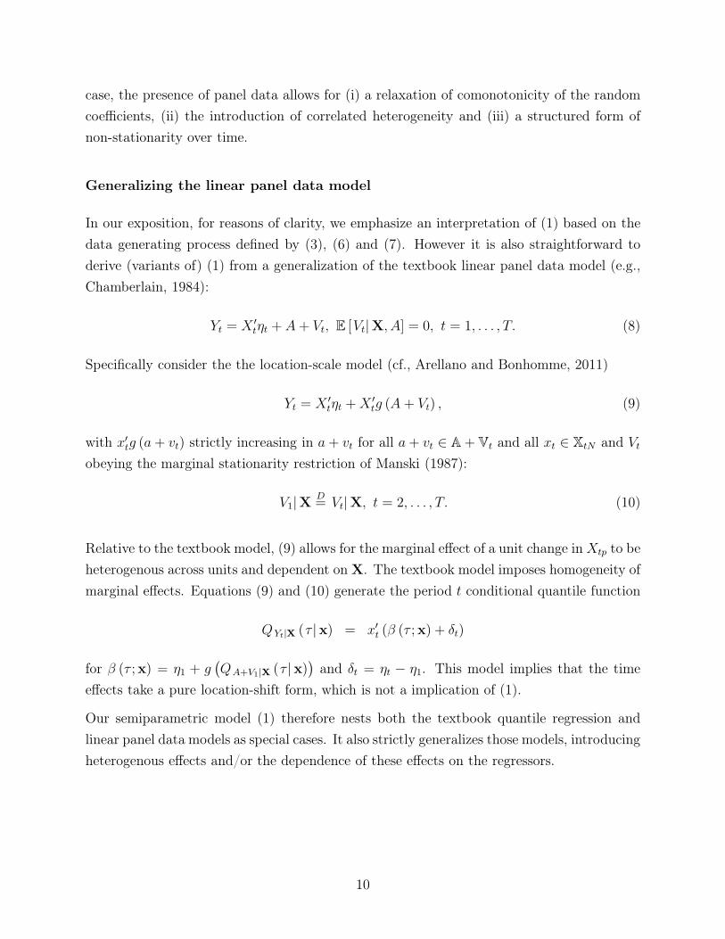
case, the presence of panel data allows for (i) a relaxation of comonotonicity of the random
coefficients, (ii) the introduction of correlated heterogeneity and (iii) a structured form of
non-stationarity over time.
Generalizing the linear panel data model
In our exposition, for reasons of clarity, we emphasize an interpretation of (1) based on the
data generating process defined by (3), (6) and (7). However it is also straightforward to
derive (variants of) (1) from a generalization of the textbook linear panel data model (e.g.,
Chamberlain, 1984):
Yt = X ′tηt + A+ Vt, E [Vt|X, A] = 0, t = 1, . . . , T. (8)
Specifically consider the the location-scale model (cf., Arellano and Bonhomme, 2011)
Yt = X ′tηt +X ′
tg (A + Vt) , (9)
with x′tg (a+ vt) strictly increasing in a+ vt for all a+ vt ∈ A+ Vt and all xt ∈ XtN and Vt
obeying the marginal stationarity restriction of Manski (1987):
V1|X D= Vt|X, t = 2, . . . , T. (10)
Relative to the textbook model, (9) allows for the marginal effect of a unit change inXtp to be
heterogenous across units and dependent on X. The textbook model imposes homogeneity of
marginal effects. Equations (9) and (10) generate the period t conditional quantile function
QYt|X (τ |x) = x′t (β (τ ;x) + δt)
for β (τ ;x) = η1 + g(QA+V1|X (τ |x)
)and δt = ηt − η1. This model implies that the time
effects take a pure location-shift form, which is not a implication of (1).
Our semiparametric model (1) therefore nests both the textbook quantile regression and
linear panel data models as special cases. It also strictly generalizes those models, introducing
heterogenous effects and/or the dependence of these effects on the regressors.
10
2 Estimands and identification
In this section we introduce three estimands based on (1). We motivate these estimands vis-
a-vis the correlated random coefficients model defined by (3), (6) and (7) above, although
this is not essential to our formal results (i.e., one could make reference to (2) directly). A
subset of our estimands only require that (1) hold for a single known τ .
Our first estimand is the R × 1 vector of common coefficients δ (τ). Recall that in our
motivating data generating process the elements of δ (τ) coincide with time effects.
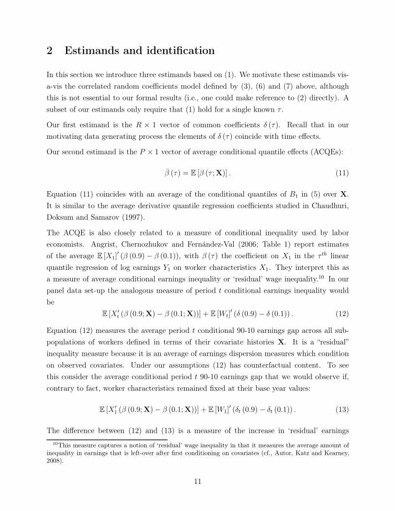
Our second estimand is the P × 1 vector of average conditional quantile effects (ACQEs):
β (τ) = E [β (τ ;X)] . (11)
Equation (11) coincides with an average of the conditional quantiles of B1 in (5) over X.
It is similar to the average derivative quantile regression coefficients studied in Chaudhuri,
Doksum and Samarov (1997).
The ACQE is also closely related to a measure of conditional inequality used by labor
economists. Angrist, Chernozhukov and Fernández-Val (2006; Table 1) report estimates
of the average E [X1]′ (β (0.9)− β (0.1)), with β (τ) the coefficient on X1 in the τ th linear
quantile regression of log earnings Y1 on worker characteristics X1. They interpret this as
a measure of average conditional earnings inequality or ‘residual’ wage inequality.10 In our
panel data set-up the analogous measure of period t conditional earnings inequality would
be
E [X ′t (β (0.9;X)− β (0.1;X))] + E [Wt]
′ (δ (0.9)− δ (0.1)) . (12)
Equation (12) measures the average period t conditional 90-10 earnings gap across all sub-
populations of workers defined in terms of their covariate histories X. It is a “residual”
inequality measure because it is an average of earnings dispersion measures which condition
on observed covariates. Under our assumptions (12) has counterfactual content. To see
this consider the average conditional period t 90-10 earnings gap that we would observe if,
contrary to fact, worker characteristics remained fixed at their base year values:
E [X ′1 (β (0.9;X)− β (0.1;X))] + E [W1]
′ (δt (0.9)− δt (0.1)) . (13)
The difference between (12) and (13) is a measure of the increase in ‘residual’ earnings
10This measure captures a notion of ‘residual’ wage inequality in that it measures the average amount ofinequality in earnings that is left-over after first conditioning on covariates (cf., Autor, Katz and Kearney,2008).
11

inequality due to changes in worker characteristics between periods 1 and t. Similar reasoning
leads to more complicated decomposition estimands.
Our final estimand is the unconditional quantile effect (UQE), defined implicitly by, for
p = 1, . . . , P,
βp (τ) = QB1p(τ)
= inf {b ∈ R : Pr (B1p ≤ b) ≥ τ}= inf {b ∈ R : Pr (βp (U1,X) ≤ b) ≥ τ}
where U1 ∼ U [0, 1], independent of X. The UQE βp (τ) corresponds to the τ th quantile of
the pth component of the random coefficient vector B1. If we took a random draw from the
population and increased her pth regressor value by one unit, then with probability τ the
effect on Y1 would be less than or equal to βp (τ), while with probability 1 − τ it would be
greater. To get the total effect for a tth period intervention, we would need to take into
account the effect on W′tδ(τ) of the change in regressor Wt (as a function of Xt).
The UQE is the quantile analog of an average partial effect (APE).
Identification
We present two sets of identification results. The first requires that the time dimension of the
panel (T ) strictly exceed the number of regressors (P ). We refer to this as the “regular” case.
Chamberlain (1992) studied identification of average partial effects in this setting. Second
we study identification when T = P . This is the case studied in Graham and Powell (2012).
We refer to this case as “irregular”. Both are empirically relevant (cf., Graham and Powell,
2012). Throughout this section we assume that the joint distribution of the observable data
matrix (Y,X) is known – in particular, that the T × 1 vector QY|X (τ |X) is known for all
τ ∈ (0, 1) and X ∈ XT .
Regular case (T > P )
Let A (X) be any T × T positive definite matrix, possibly a function of X, and define the
residual-maker matrix
MA (X) = IT −X (X′A (X)X)−1
X′A (X) . (14)
12

If E [‖X‖2 + ‖W‖2] <∞ and E [W′MA(X)W] is invertible we can recover δ (τ) by
δ (τ) = E [W′MA (X)W]−1 × E
[W
′MA (X)QY|X (τ |X)]. (15)
Equation (15) shows that δ (τ) indexes a (generalized) within-unit, double residual, linear
regression function. The dependent variable associated with this regression is QYt|X (τ |X)
deviated from its unit-specific “mean” and the independent variable the deviation of Wt
about its corresponding “mean” . Chamberlain (1992, Section 4) introduced transformations
of this type in the panel context (cf., Graham and Powell (2012)). Bajari, Hahn, Hong and
Ridder (2011) use a similar transformation to study identification in incomplete information
games.
Once δ(τ) is identified, we can also identify the τ th conditional quantile of the random
coefficient, for X realizations with full rank, through the relation
β(τ ;X) = (X′A (X)X)−1
X′A (X) (QY|X(τ |X)−Wδ(τ)). (16)
If all realizations of X are of full rank, we can directly recover the average conditional quantile
effect (ACQE) from (16) by
β(τ) = E [β(τ ;X)]
= E
[(X′A (X)X)
−1X
′A (X) (QY|X(τ |X)−Wδ(τ))], (17)
while the unconditional quantile βp(τ) of the pth component of B1 is identified as the solution
to the equation
E [1(βp(U ;X) ≤ βp(τ))− τ ] = 0, (18)
with U uniformly distributed on (0, 1), independently from X. The UQE βp(τ) will be
uniquely identified if the distribution of β(U ;X) is continuous around its τ th quantile with
positive density.
Equations (17) and (18) do not follow if the probability π0 that X is rank deficient is strictly
positive. Denote by XM the region of the support of X where its rank is full, and denote
by π0 the probability that the rank of X is less than P . When π0 > 0 it is still possible to
identify δ(τ), by using the observations where X ∈ XM , via
δ(τ) = E[W
′MA(X)W|X ∈ XM]−1 × E
[W
′MA(X)QY|X(τ |X)|X ∈ XM],
if we now assume that E[W
′MA(X)W|X ∈ XM]
is invertible and under the same moments
13
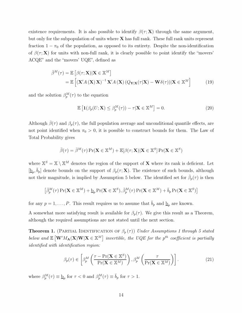
existence requirements. It is also possible to identify β(τ ;X) through the same argument,
but only for the subpopulation of units where X has full rank. These full rank units represent
fraction 1 − π0 of the population, as opposed to its entirety. Despite the non-identification
of β(τ ;X) for units with non-full rank, it is clearly possible to point identify the “movers’
ACQE” and the “movers’ UQE”, defined as
βM(τ) = E[β(τ ;X)|X ∈ X
M]
= E
[(X′A (X)X)
−1X
′A (X) (QY|X(τ |X)−Wδ(τ))|X ∈ XM]
(19)
and the solution βMp (τ) to the equation
E[1(βp(U ;X) ≤ βMp (τ))− τ |X ∈ X
M]= 0. (20)
Although β(τ) and βp(τ), the full population average and unconditional quantile effects, are
not point identified when π0 > 0, it is possible to construct bounds for them. The Law of
Total Probability gives
β(τ) = βM(τ) Pr(X ∈ XM) + E[β(τ ;X)|X ∈ X
S] Pr(X ∈ XS)
where XS = X \ XM denotes the region of the support of X where its rank is deficient. Let
[bp, bp] denote bounds on the support of βp(τ ;X). The existence of such bounds, although
not their magnitude, is implied by Assumption 5 below. The identified set for βp(τ) is then
[βMp (τ) Pr(X ∈ X
M) + bp Pr(X ∈ XS), βMp (τ) Pr(X ∈ X
M) + bp Pr(X ∈ XS)]
for any p = 1, . . . , P . This result requires us to assume that bp and bp are known.
A somewhat more satisfying result is available for βp(τ). We give this result as a Theorem,
although the required assumptions are not stated until the next section.
Theorem 1. (Partial Identification of βp (τ)) Under Assumptions 1 through 5 stated
below and E[W
′MA(X)W|X ∈ XM]
invertible, the UQE for the pth coefficient is partially
identified with identification region:
βp(τ) ∈[βMp
(τ − Pr(X ∈ XS)
Pr(X ∈ XM)
), βMp
(τ
Pr(X ∈ XM)
)]. (21)
where βMp (τ) ≡ bp for τ < 0 and βMp (τ) ≡ bp for τ > 1.
14

Proof. See Appendix B.
Since the movers’ UQE is identified, as well as Pr(X ∈ XM) and Pr(X ∈ X
S) = 1− Pr(X ∈XM), the analog estimators for the lower and upper bounds of the identified set given in
(21) are easy to compute.11 If prior bounds on the random coefficient are unknown, these
bounds are only meaningful for τ in a subset of (0, 1). The width of this subset depends on
the fraction of stayers. When τ is close to either 0 or 1, we must rely on prior bounds bp and
bp to set identify the UQE, as is the case for the ACQE.
Irregular case (T = P )
We now consider the T = P case. Our approach builds on that of Graham and Powell (2012)
for average effects in a conditional mean variant of (1). While identification in the regular
case is based solely on the subpopulation of movers, the irregular case utilizes both movers
and stayers. The role of stayers is to identify the common parameter δ (τ), which in our
motivating data generating process, captures aggregate time effects. Stayers, as we detail
below, serve as a type of control group, allowing the econometrician to identify “common
trends” affecting all units.
Let D = det(X), X∗ denote the adjugate (or adjoint) matrix of X (i.e., the matrix such that
X−1 = 1
DX
∗ when D 6= 0), and W∗ = X
∗W. Premultiplying equation (1) by X
∗ gives
X∗QY|X(τ |X) = W
∗δ(τ) +Dβ(τ ;X). (22)
Assuming that zero is in the support of the determinant, D, E [‖W∗‖2] < ∞ and that
E[W∗′W
∗|D = 0] is of full rank, we can identify δ(τ), using only stayer (i.e., D = 0)
observations, by:
δ(τ) = E [W∗′W
∗|D = 0]−1 × E
[W
∗′X
∗QY|X(τ |X)|D = 0]. (23)
Given identification of δ(τ), we can then recover β(τ ;X) by
β(τ ;X) = X−1(QY|X(τ |X)−Wδ(τ)) (24)
for all X where X−1 = 1
DX
∗ is well-defined (i.e., for “mover” realizations of X).
11The endpoints’ joint asymptotic distribution can be readily inferred from the process convergence of theUQE process established below.
15

As long as Pr (D = 0) = 0 it follows that the conditional effect β(τ ;X) will be identified
with probability one. However, the identification of the ACQE and UQE estimands is more
delicate than in the regular case, due to the fact that if the density of D is positive in
a neighborhood of 0 (which we require for identification of δ(τ)), expectations involving
X−1 = 1
DX
∗ will not exist in general (e.g., Khan and Tamer (2010) and Graham and Powell
(2012)). In order to identify the ACQE, β(τ), we write it as the limit of a sequence of
“trimmed” expectations
β(τ) = E[β(τ ;X)]
= limh↓0
E[β(τ ;X)1(|D| > h)]
= limh↓0
E[X−1(QY|X(τ |X)−Wδ(τ))1(|D| > h)], (25)
where the second equality holds because
β(τ)− E[β(τ ;X)1(|D| > h)] = E[β(τ ;X)1(|D| ≤ h)] = O(h)
under sufficient smoothness conditions. This trimming is not strictly necessary at the iden-
tification stage, under the maintained assumption that β(τ) exists, but is introduced in
anticipation of its estimation. In particular, replacing QY|X(τ |X) with a nonparametric esti-
mate introduces noise into the numerator of the sample analog of (25). This sampling error
may cause the expectation of the estimated conditional effect
β(τ ;X) = X−1(QY|X(τ |X)−Wδ(τ))
to be undefined due to a lack of moments of the remainder term
β(τ ;X)− β(τ ;X) = X−1(QY|X(τ |X)−QY|X(τ |X)−W(δ(τ)− δ(τ))
).
We can also characterize the identification of βp(τ), the UQE associated with the pth regres-
sor, in terms of a sequence of trimmed means. Assuming that the distribution of β(U ;X)
given D = t is continuously differentiable in a neighborhood of t = 0, we can write βp(τ) as
the solution to
0 = E [1(βp(U ;X) ≤ βp(τ))− τ ]
= limh↓0
E [(1(βp(U ;X) ≤ βp(τ))− τ)1(|D| > h)] .
16

Our approach to estimation exploits this characterization.
If there is a point mass of stayer units with D = 0 (i.e. π0 > 0), the same identification
issues arise here as in the regular (T > P ) case. In this case we can continue to identify δ(τ)
as before, but β(τ ;X) will be unidentified for a set of X values with positive probability. It
is still possible identify the movers’ ACQE and UQE using straightforward modifications of
the arguments given for the regular case in the previous subsection.
As a simple example of irregular identification consider a two period version of (1) with a
single time-varying regressor (X2t) and an intercept time shift.12 This setup yields conditional
quantiles for each period of
QY1|X(τ |x) = β1 (τ ;x) + β2 (τ ;x)X21
QY2|X(τ |x) = δ (τ) + β1 (τ ;x) + β2 (τ ;x)X22.
Here X2t might be a policy variable, such as an individuals’ workers compensation benefit
level, which depends on own earnings as well as state-specific benefit schedules, and Yt an
outcome of interest to a policymaker, such as time out of work following an injury.
Evaluating (23) we get
δ (τ) = E[ω (X21)
{QY2|X(τ |X)−QY1|X(τ |X)
}∣∣D = 0], ω (X1) =
1 +X221
E [1 +X221|D = 0]
,
so that δ (τ) is identified by a weighted average of changes in the τ th quantile of Yt between
periods 1 and 2 across the subpopulation of stayers. Stayer units, who in this case correspond
to units where X21 = X22 (i.e., the nonconstant regressor stays fixed over time), serve as a
type of “control group”, identifying aggregate time effects or “common trends”.
The conditional quantile effect of a unit change in X2t is given by the second element of (24),
which evaluates to
βp (τ ;x) =QY2|X(τ |x)−QY1|X(τ |x)− δ (τ)
△x2,
for all x with x22−x22 = △x2 6= 0. Hence βp (τ ;x) is identified by a “difference-in-differences”.
12This corresponds to (1) with T = P = 2 and W and X equal to
W =
(01
), X =
(1 X21
1 X22
)
so that D = X22 −X21 = △X2.
17
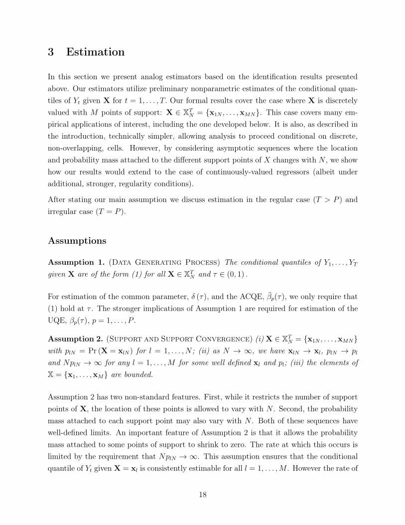
3 Estimation
In this section we present analog estimators based on the identification results presented
above. Our estimators utilize preliminary nonparametric estimates of the conditional quan-
tiles of Yt given X for t = 1, . . . , T. Our formal results cover the case where X is discretely
valued with M points of support: X ∈ XTN = {x1N , . . . ,xMN}. This case covers many em-
pirical applications of interest, including the one developed below. It is also, as described in
the introduction, technically simpler, allowing analysis to proceed conditional on discrete,
non-overlapping, cells. However, by considering asymptotic sequences where the location
and probability mass attached to the different support points of X changes with N , we show
how our results would extend to the case of continuously-valued regressors (albeit under
additional, stronger, regularity conditions).
After stating our main assumption we discuss estimation in the regular case (T > P ) and
irregular case (T = P ).
Assumptions
Assumption 1. (Data Generating Process) The conditional quantiles of Y1, . . . , YT
given X are of the form (1) for all X ∈ XTN and τ ∈ (0, 1) .
For estimation of the common parameter, δ (τ), and the ACQE, βp(τ), we only require that
(1) hold at τ . The stronger implications of Assumption 1 are required for estimation of the
UQE, βp(τ), p = 1, . . . , P .
Assumption 2. (Support and Support Convergence) (i) X ∈ XTN = {x1N , . . . ,xMN}
with plN = Pr (X = xlN) for l = 1, . . . , N ; (ii) as N → ∞, we have xlN → xl, plN → pl
and NplN → ∞ for any l = 1, . . . ,M for some well defined xl and pl; (iii) the elements of
X = {x1, . . . ,xM} are bounded.
Assumption 2 has two non-standard features. First, while it restricts the number of support
points of X, the location of these points is allowed to vary with N . Second, the probability
mass attached to each support point may also vary with N . Both of these sequences have
well-defined limits. An important feature of Assumption 2 is that it allows the probability
mass attached to some points of support to shrink to zero. The rate at which this occurs is
limited by the requirement that NplN → ∞. This assumption ensures that the conditional
quantile of Yt given X = xl is consistently estimable for all l = 1, . . . ,M . However the rate of
18

convergence of these estimates will be slower for points of support with shrinking probability
mass as N grows large.13
For the analysis which follows it is convenient to partition the support of X as follows.
1. Units with X = xmN for m = 1, . . . , L1 < M correspond to movers. Movers cor-
respond to units where, recalling that xmN → xm, xm and xmN are of full rank.
Intuitively movers are units whose covariate values “vary a lot” over time.
2. Units with X = xmN for m = L1 + 1, . . . , L < M correspond to near stayers. Near
stayers correspond to units where xmN is of full rank, but its limit xm is not. We will
be more precise about the behavior of these units’ design matrices along the path to
the limit below. Intuitively near stayers are units who covariate values change “very
little” over time.
3. Units with X = xmN for m = L + 1, . . . ,M correspond to stayers. Stayers are units
where xmN is neither of full rank along the path nor in the limit. Stayers correspond
to units where the number of distinct rows of X is less than P (i.e., whose regressor
sequences display substantial persistence).
We let XMN = {x1N , . . .xLN} denote the set of mover support points (including near stayers).
The set of stayer support points is denoted by XSN = {xL+1N , . . .xMN}. We introduce more
structure to this basic set-up (as needed) below.
Assumption 3. (Random Sampling) {Yi,Xi}Ni=1 is a random (i.i.d.) sample from the
population of interest.
Assumption 4. (Bounded and Continuous Densities) The conditional distribution
FYt|X (yt|x) has density fYt|X (yt|x) such that ψ (τ ;x) = fYt|X
(F−1Yt|X
(τ |x)∣∣∣x)
and ∂ψ(τ ;x)∂τ
are uniformly bounded and bounded away from zero for all τ ∈ (0, 1), all x ∈ XTN , and
all t = 1, . . . , T. Also, this conditional distribution does not vary with the sample size N .
Finally, fYt|X (yt|x), FYt|X (yt|x) and F−1Yt|X
(yt|x) are all continuous in x.
Assumption 5. (Bounded Coefficients) The support of Btp is compact and its density
is bounded away from 0 for any p = 1, . . . , P and t = 1, . . . , T .
Assumptions 3 is standard, as is Assumption 4 is the quantile regression context. Assumption
5, in conjunction with Assumption 2 ensures that Y has bounded support.
13Also note that, since W is a function of X alone, it too has M points of support: W ∈ WTN =
{w1N , . . . ,wMN} .
19
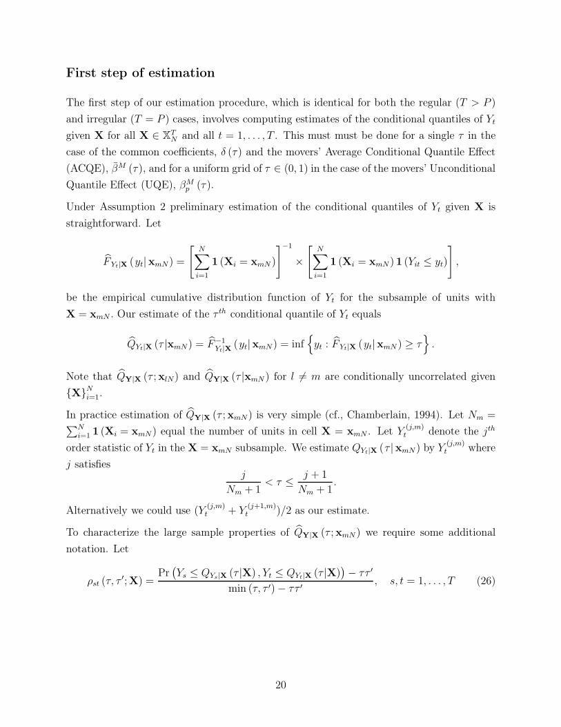
First step of estimation
The first step of our estimation procedure, which is identical for both the regular (T > P )
and irregular (T = P ) cases, involves computing estimates of the conditional quantiles of Yt
given X for all X ∈ XTN and all t = 1, . . . , T . This must must be done for a single τ in the
case of the common coefficients, δ (τ) and the movers’ Average Conditional Quantile Effect
(ACQE), βM (τ), and for a uniform grid of τ ∈ (0, 1) in the case of the movers’ Unconditional
Quantile Effect (UQE), βMp (τ).
Under Assumption 2 preliminary estimation of the conditional quantiles of Yt given X is
straightforward. Let
FYt|X (yt|xmN ) =[
N∑
i=1
1 (Xi = xmN )
]−1
×[
N∑
i=1
1 (Xi = xmN ) 1 (Yit ≤ yt)
],
be the empirical cumulative distribution function of Yt for the subsample of units with
X = xmN . Our estimate of the τ th conditional quantile of Yt equals
QYt|X (τ |xmN ) = F−1Yt|X
(yt|xmN ) = inf{yt : FYt|X (yt|xmN ) ≥ τ
}.
Note that QY|X (τ ;xlN) and QY|X (τ |xmN ) for l 6= m are conditionally uncorrelated given
{X}Ni=1.
In practice estimation of QY|X (τ ;xmN ) is very simple (cf., Chamberlain, 1994). Let Nm =∑N
i=1 1 (Xi = xmN ) equal the number of units in cell X = xmN . Let Y(j,m)t denote the jth
order statistic of Yt in the X = xmN subsample. We estimate QYt|X (τ |xmN ) by Y(j,m)t where
j satisfiesj
Nm + 1< τ ≤ j + 1
Nm + 1.
Alternatively we could use (Y(j,m)t + Y
(j+1,m)t )/2 as our estimate.
To characterize the large sample properties of QY|X (τ ;xmN ) we require some additional
notation. Let
ρst (τ, τ′;X) =
Pr(Ys ≤ QYs|X (τ |X) , Yt ≤ QYt|X (τ |X)
)− ττ ′
min (τ, τ ′)− ττ ′, s, t = 1, . . . , T (26)
20
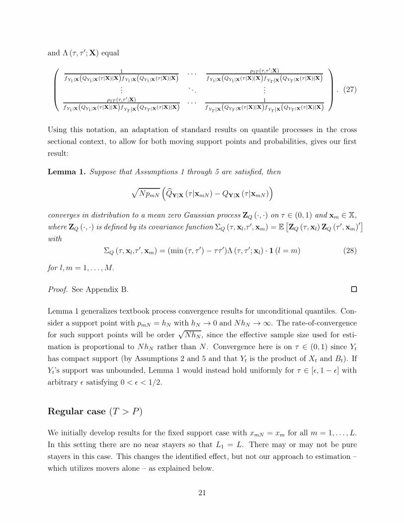
and Λ (τ, τ ′;X) equal
1
fY1|X(QY1|X(τ |X)|X)fY1|X(QY1|X
(τ |X)|X)· · · ρ1T (τ,τ ′;X)
fY1|X(QY1|X(τ |X)|X)fYT |X(QYT |X(τ |X)|X)
.... . .
...ρ1T (τ,τ ′;X)
fY1|X(QY1|X(τ |X)|X)fYT |X(QYT |X(τ |X)|X)
· · · 1
fYT |X(QYT |X(τ |X)|X)fYT |X(QYT |X(τ |X)|X)
. (27)
Using this notation, an adaptation of standard results on quantile processes in the cross
sectional context, to allow for both moving support points and probabilities, gives our first
result:
Lemma 1. Suppose that Assumptions 1 through 5 are satisfied, then
√NpmN
(QY|X (τ |xmN )−QY|X (τ |xmN )
)
converges in distribution to a mean zero Gaussian process ZQ (·, ·) on τ ∈ (0, 1) and xm ∈ X,
where ZQ (·, ·) is defined by its covariance function ΣQ (τ,xl,τ′,xm) = E
[ZQ (τ,xl)ZQ (τ ′,xm)
′]
with
ΣQ (τ,xl,τ′,xm) = (min (τ, τ ′)− ττ ′)Λ (τ, τ ′;xl) · 1 (l = m) (28)
for l, m = 1, . . . ,M.
Proof. See Appendix B.
Lemma 1 generalizes textbook process convergence results for unconditional quantiles. Con-
sider a support point with pmN = hN with hN → 0 and NhN → ∞. The rate-of-convergence
for such support points will be order√NhN , since the effective sample size used for esti-
mation is proportional to NhN rather than N . Convergence here is on τ ∈ (0, 1) since Yt
has compact support (by Assumptions 2 and 5 and that Yt is the product of Xt and Bt). If
Yt’s support was unbounded, Lemma 1 would instead hold uniformly for τ ∈ [ǫ, 1 − ǫ] with
arbitrary ǫ satisfying 0 < ǫ < 1/2.
Regular case (T > P )
We initially develop results for the fixed support case with xmN = xm for all m = 1, . . . , L.
In this setting there are no near stayers so that L1 = L. There may or may not be pure
stayers in this case. This changes the identified effect, but not our approach to estimation –
which utilizes movers alone – as explained below.
21

Let Π(τ) = (QY|X(τ |x1)′, . . . , QY|X(τ |xL)′)′ be a TL × 1 vector with movers’ conditional
quantiles and notice that, under (1),
Π(τ) = Gγ(τ)
for τ ∈ (0, 1) with
γ (τ)(R+PL)×1
=
δ (τ)
β (τ ;x1)...
β (τ ;xL)
, G
TL×(R+PL)=
w1 x1 · · · 0T0′P
......
. . ....
wL 0T0′P · · · xL
. (29)
Since rank (G) = dim (γ (τ)) we have
γ (τ) = (G′AG)−1G′AΠ (τ) , (30)
for any TL× TL positive-definite weight matrix A.
When A is block diagonal with mth T × T block pmA (xm) , it is straightforward to demon-
strate that the first R elements of γ(τ) in (30) can be expressed as
δ(τ) = E[W
′MA(X)W|X ∈ XM]−1 × E
[W
′MA(X)QY|X(τ |X)|X ∈ XM],
which coincides with (15) above. Manipulation of (30) also yields, for all X ∈XM ,
β (τ ;X) = [X′A (X)X]−1
X′A (X)
(QY|X(τ |X)−Wδ (τ)
),
which coincides with (16) above.
Our analog estimator is
γ(τ) = (G′AG)−1G′AΠ(τ) (31)
where A is a consistent estimator of a positive definite weight matrix and Π(τ) is as defined
above. To get precise results we make the following assumption on the weight matrix.
Assumption 6. (Weight Matrix) A = diag{p1N , . . . , pLN}⊗IT where pl =1N
∑Ni=1 1(Xi =
xlN).
This assumption is made to simplify the analysis and because weighting each support point
by its relative frequency is often a reasonable choice. Although we do not develop this point
22

here, it is straightforward to show, by adapting the argument given by Chamberlain (1994),
that this choice of weight matrix also allows for easy characterization of the large sample
properties of γ(τ) under misspecification (i.e., when (1) does not hold).
Define
W =MI (X)W, MI (X) = IT −X (X′X)
−1X
′
K (X) = (X′X)
−1X
′W, Γ = E
[W
′W
∣∣∣X ∈ XM].
Theorem 2. Suppose that Assumptions 1 through 6 are satisfied, the distribution of X is
fixed, and E
[W
′W|X ∈ XM
]is invertible, then (i)
√N(δ (·)− δ (·)
)converges in distribu-
tion to a mean zero Gaussian process Zδ (·), where Zδ (·) is defined by its covariance function
Σδ(τ, τ′) = E[Zδ (τ)Zδ (τ
′)′] = (min (τ, τ ′)− ττ ′)
Γ−1E
[W
′Λ (τ, τ ′;X)W
∣∣∣X ∈ XM]Γ−1
P(X ∈ XM),
(32)
and (ii)√N(β (·; ·)− β (·; ·)
)also converges in distribution to a mean zero Gaussian process
Z (·, ·), where Z (·, ·) is defined by its covariance function
Σ(τ,xl, τ′,xm) = E
[Z (τ,xl)Z (τ ′,xm)
′]
= (min (τ, τ ′)− ττ ′)(x′
lxl)−1
x′lΛ (τ, τ ′;xl)xl (x
′lxl)
−1
pl· 1 (l = m)
+K (xl) Σδ(τ, τ′)K (xm)
′ , (33)
for l, m = 1, . . . , L.
Proof. See Appendix B.
When X has finite support and, as maintained here, the location and probability mass
attached to this support does not change with N , the rate of convergence of β (τ ;xm) and
δ (τ) is√N . At the same time it is not possible to identify β(τ ;xm) for the stayer realizations
m = L+1, . . . ,M . Hence under the fixed support assumption β(τ), the average conditional
quantile effect, is not point identified. However, the movers’ ACQE, defined as βM(τ) =
E[β(τ ;X)|X ∈ XM ], is consistently estimable by
βM
(τ) =
∑Ni=1 1
(Xi ∈ XM
)β (τ ;Xi)∑N
i=1 1 (Xi ∈ XM). (34)
23

Theorem 3. Under the assumptions maintained in Theorem 2 above,√N(β
M
(·)− βM(·))
converges in distribution to a mean zero Gaussian process Zβ (·), where Zβ (·) is defined by
its covariance function
Σβ(τ, τ′) = E
[Zβ (τ)Zβ (τ
′)′]
=C(β (τ ;X) , β (τ ′;X)′
∣∣X ∈ XM)
P (X ∈ XM)+ Υ1(τ, τ
′) +KMΣδ(τ, τ′)KM ′ (35)
where
Υ1 (τ, τ′) =
(min (τ, τ ′)− ττ ′)
P(X ∈ XM)E
[(X′
X)−1
X′Λ (τ, τ ′;X)X (X′
X)−1 |X ∈ X
M],
KM = E[K(X)|X ∈ XM ].
Proof. See Appendix B.
The first term in the asymptotic distribution of βM
(τ) arises from variation in the random
coefficients across the subpopulation of movers. The second and third terms reflect sampling
uncertainty in β(τ ;x) and δ(τ) respectively (which arises because the conditional distribution
of Y given X is unknown). The form of Σβ(τ, τ′) mirrors that derived by Chamberlain (1992)
for averages of random coefficients.
As with the ACQE, unconditional quantile effects are only identified across the subpopulation
of movers. Our estimate of βMp (τ) is given by the solution to the empirical counterpart of
(20) above
N∑
i=1
1(Xi ∈ X
M){ˆ u=1
u=0
[1(βp(u;Xi) ≤ βMp (τ))− τ
]du
}= 0. (36)
The integral in (36) can be calculated exactly since βp(u;xl) is piecewise linear for each
xl with finitely many pieces. Alternatively it may be approximated by a finite sum of the
integrand evaluated at H evenly spaced points u1, . . . , uH between zero and one. In that case
βMp (τ) has a simple order statistic representation. Let NMOVER =∑N
i=1 1(Xi ∈ XM
)equal
the number of movers in the sample and construct the list
{{βp(uh;Xi)
}Hh=1
}NMOVER
i=1
.14 The
14We assume, without loss of generality, that the sample is ordered such that mover realizations appearfirst with indices i = 1, . . . , NMOVER.
24

jth order statistic of this list is our estimate of βMp (τ) where j satisfies
j
HNMOVER + 1< τ ≤ j + 1
HNMOVER + 1.
Theorem 4. Under the assumptions maintained in Theorem 2 above√N(βMp (·)− βMp (·)
)
converges in distribution to a mean zero Gaussian process Zβp (·), where Zβp (·) is defined by
its covariance function, Σβp(τ, τ′)
Σβp(τ, τ′) =
1
P (X ∈ XM)
Υ2 (τ, τ′) + Υ3 (τ, τ
′) + Υ4 (τ, τ′)
fBp|X∈XM
(βMp (τ)
∣∣X ∈ XM)fBp|X∈XM
(βMp (τ ′)
∣∣X ∈ XM) , (37)
where
Υ2(τ, τ′) =
C(FBp|X(β
Mp (τ)|X), FBp|X(β
Mp (τ ′)|X)|X ∈ XM
)
P (X ∈ XM), (38)
Υ3(τ, τ′) = P
(X ∈ X
M)−1
E[(min
(FBp|X(β
Mp (τ)|X), FBp|X(β
Mp (τ ′)|X)
)
−FBp|X(βMp (τ)|X)FBp|X(β
Mp (τ ′)|X)
)
× e′p (X′X)
−1X
′Λ(FBp|X(β
Mp (τ)|X), FBp|X(β
Mp (τ ′)|X);X
)X (X′
X)−1ep
×fBp|X(βMp (τ)|X)fBp|X(β
Mp (τ ′)|X)
∣∣X ∈ XM], (39)
and
Υ4(τ, τ′) = e′p
(ˆ ˆ [
fBp|X(βMp (τ)|x)fBp|X(β
Mp (τ ′)|x)
×K (x) Σδ(FBp|X(β
Mp (τ)|x), FBp|X(β
Mp (τ ′)|x)
)K (x)′
]
×fX|X∈XM
(x|x ∈ X
M)fX|X∈XM
(x| x ∈ X
M)dm(x)dm(x)
)ep (40)
with ep a P × 1 vector with a 1 in its pth row and zeros elsewhere.
Proof. See Appendix B.
While the form of the covariance function Σβp(τ, τ′) is complicated, each term in it has
a straightforward interpretation. The Υ2(·) term reflects sampling variability arising from
the econometrician’s lack of knowledge of the marginal distribution of X. It would also be
zero if the distribution of Bp|X = x were constant across all x ∈ XM (i.e., no correlated
heterogeneity). This term is analogous to the first term appearing the covariance expression
25

for the ACQE in Theorem 3 above. The Υ3(·) term measures estimation error associated with
a lack of knowledge of the distribution of Y given X; specifically it captures the influence
of sampling error in conditional quantiles of Yt on the sampling variability of the estimated
UQE. The Υ4(·) term is due to the estimation of the common coefficient δ(·).15
Irregular case (T = P )
Our estimation procedure for the regular T > P case only utilizes information on movers.
Our analysis of the irregular T = P case additionally utilizes information on stayers and near
stayers, making full use of the possibilities implied by Assumption 2. In the irregular case,
similar to Graham and Powell (2012), estimation of the common coefficient, δ (τ), requires
the availability of stayers and/or near stayers.
We introduce the presence of near stayers to illustrate how the population-wide ACQE and
UQE, not just their movers’ counterparts, may be consistently estimated.
Our analysis relies on “discrete bandwidth asymptotics”, we argue that our approach, in
addition to being of value on its own terms, approximates many features of an analysis with
continuously-valued covariates. To motivate this claim we begin by reproducing the results
of Graham and Powell (2012) (which used a linear model for conditional expectations instead
of quantiles and imposed continuity of some components of X).
Discrete bandwidth framework
We first outline the discrete bandwidth framework we use for the T = P case; adding
maintained details to the basic set-up outlined in Assumption 2. With T = P , the X matrix
is square, with full rank if and only if detX 6= 0. Recall that D = detX and suppose that
D ∈ DN = {d1, . . . , dK ,−hN , hN , 0}, the support of the determinant of X. The first K
elements of DN correspond to the L1 mover support points of X. The next two elements
of DN correspond to the L−L1 near stayer support points of X. The final element of DN
corresponds to the M − L stayer support points of X.
We set Pr(D = hN ) = Pr(D = −hN ) = φ0hN for some φ0 ≥ 0, defining dK+1,N = −hN ,
dK+2,N = hN and dK+3 = 0. The mover support points dk for 1 ≤ k ≤ K are bounded away
from 0 for all N .
15Note the measure in Υ4 (·) is the counting measure.
26

We also set the probability of observing a singular X be Pr(D = 0) = 2φ0hN . Finally,
Pr(D = dk) = πNk for k = 1, . . . , K with∑K
k=1 πNk = 1 − 4φ0hN , with 4φ0hN < 1 for all N .
We also let πk = limN→∞ πNk , so that∑K
k=1 πk = 1.16
In this setup, observations with D = 0 are stayers, D = ±hN are near-stayers, while those
with D = dk for k = 1, . . . , K correspond to movers. The inclusion of near-stayers is a way
to approximate a continuous distribution of D, letting near stayers (those with D = ±hN )
have characteristics very similar to those of stayers (D = 0).
Let qmN |k = Pr(X = xmN |D = dk), qmN |−h = Pr(X = xmN |D = −hN ), qmN |h = Pr(X =
xmN |D = hN) and qmN |0 = Pr(X = xmN |D = 0). For simplicity, we assume that qmN |· does
not vary with N , so that conditional on the value of the determinant, which has varying
support, the distribution of X does not depend on the sample size. We also assume that
limN→∞
qm|h = limN→∞
qm|−h = qm|0 for all m = 1, . . . ,M . This is a smoothness assumption.
In what follows recall that X∗ = adj (X) denotes the adjoint of X such that X−1 = 1DX
∗,when
X−1 exists and also that Y∗ = X
∗Y and W
∗ = X∗W.
Average partial effects under discrete bandwidth asymptotics
To illustrate the operation of our discrete bandwidth framework in a familiar setting we
revisit the conditional mean model studied by Graham and Powell (2012):
E[Y|X] = Wδ0 +Xβ0(X).
For the case where Xt is continuously-valued, T = P , and other maintained assumptions,
Graham and Powell (2012) estimate δ0 and the average β0 = E[β(X)] by (cf., equations (24)
and (25) in their paper).
δ =
(1
Nh
N∑
i=1
W∗′i W
∗i1(|Di| < hN )
)−1(1
Nh
N∑
i=1
W∗′i Y
∗i 1(|Di| < hN )
)(41)
β =1N
∑Ni=1X
−1i (Yi −Wiδ)1(|Di| ≥ hN)
1N
∑Ni=1 1(|Di| ≥ hN )
(42)
where Y∗i = X
∗iYi.
17
16The πk are well defined limits by Assumption 2.17Note that, relative to their expressions, we have changed the definition of stayers from units with
|Di| ≤ hN to units with |Di| < hN and conversely for movers. This change has no impact when D iscontinuously distributed, and is made here to allow the near-stayers in our framework to be categorized asmovers rather than stayers.
27
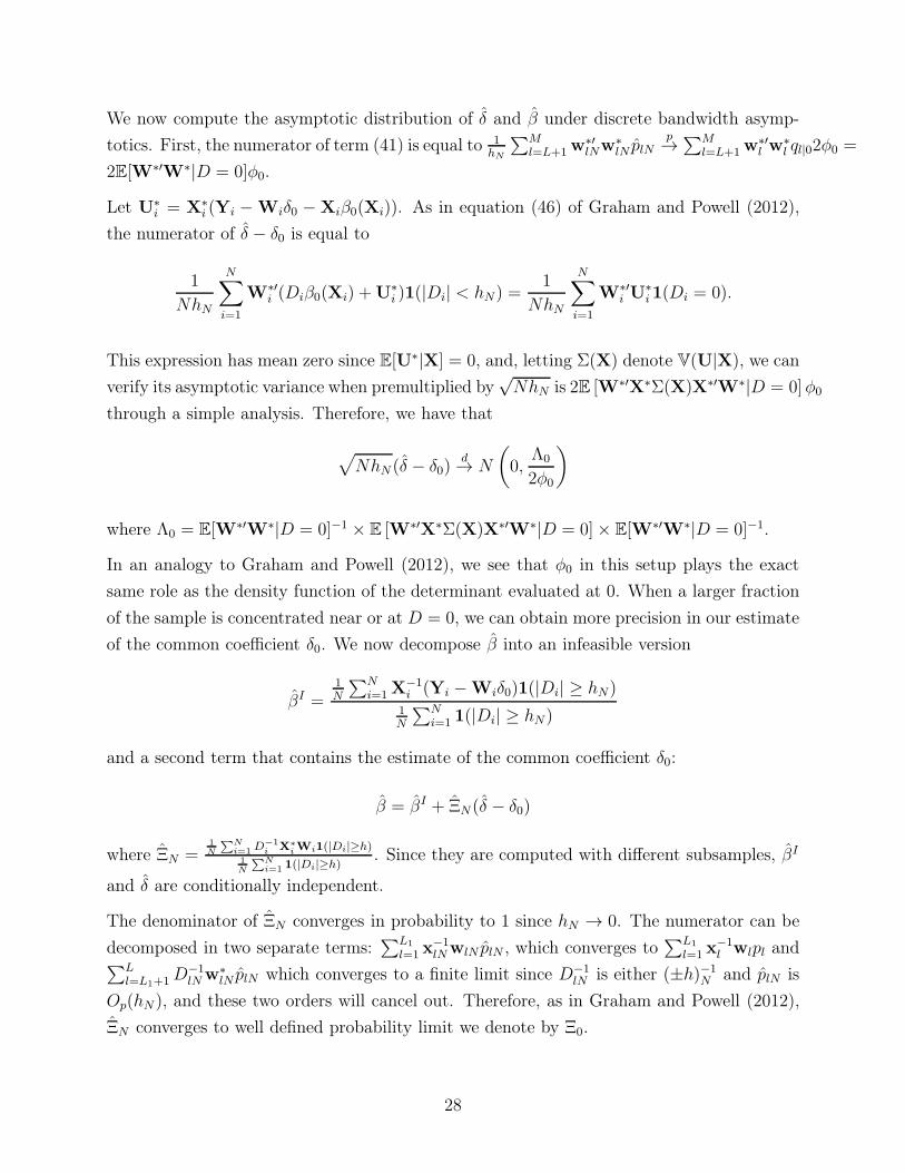
We now compute the asymptotic distribution of δ and β under discrete bandwidth asymp-
totics. First, the numerator of term (41) is equal to 1hN
∑Ml=L+1w
∗′lNw
∗lN plN
p→∑Ml=L+1w
∗′l w
∗l ql|02φ0 =
2E[W∗′W
∗|D = 0]φ0.
Let U∗i = X
∗i (Yi − Wiδ0 −Xiβ0(Xi)). As in equation (46) of Graham and Powell (2012),
the numerator of δ − δ0 is equal to
1
NhN
N∑
i=1
W∗′i (Diβ0(Xi) +U
∗i )1(|Di| < hN) =
1
NhN
N∑
i=1
W∗′i U
∗i1(Di = 0).
This expression has mean zero since E[U∗|X] = 0, and, letting Σ(X) denote V(U|X), we can
verify its asymptotic variance when premultiplied by√NhN is 2E [W∗′
X∗Σ(X)X∗′
W∗|D = 0]φ0
through a simple analysis. Therefore, we have that
√NhN (δ − δ0)
d→ N
(0,
Λ0
2φ0
)
where Λ0 = E[W∗′W
∗|D = 0]−1 × E [W∗′X
∗Σ(X)X∗′W
∗|D = 0]× E[W∗′W
∗|D = 0]−1.
In an analogy to Graham and Powell (2012), we see that φ0 in this setup plays the exact
same role as the density function of the determinant evaluated at 0. When a larger fraction
of the sample is concentrated near or at D = 0, we can obtain more precision in our estimate
of the common coefficient δ0. We now decompose β into an infeasible version
βI =1N
∑Ni=1X
−1i (Yi −Wiδ0)1(|Di| ≥ hN)
1N
∑Ni=1 1(|Di| ≥ hN)
and a second term that contains the estimate of the common coefficient δ0:
β = βI + ΞN (δ − δ0)
where ΞN =1
N
∑Ni=1
D−1i X∗
iWi1(|Di|≥h)1
N
∑Ni=1
1(|Di|≥h). Since they are computed with different subsamples, βI
and δ are conditionally independent.
The denominator of ΞN converges in probability to 1 since hN → 0. The numerator can be
decomposed in two separate terms:∑L1
l=1 x−1lNwlN plN , which converges to
∑L1
l=1 x−1l wlpl and∑L
l=L1+1D−1lNw
∗lN plN which converges to a finite limit since D−1
lN is either (±h)−1N and plN is
Op(hN ), and these two orders will cancel out. Therefore, as in Graham and Powell (2012),
ΞN converges to well defined probability limit we denote by Ξ0.
28

Finally, we see that
βI − β0 =1N
∑Ni=1(β0(Xi)− β0)1(|Di| ≥ hN )
1N
∑Ni=1 1(|Di| ≥ hN)
+1N
∑Ni=1D
−1i U
∗i1(|Di| > hN)
1N
∑Ni=1 1(|Di| ≥ hN)
+1N
∑Ni=1D
−1i U
∗i1(|Di| = hN)
1N
∑Ni=1 1(|Di| ≥ hN)
.
The denominators of both terms above, 1N
∑Ni=1 1(|Di| ≥ h), converge to 1 since the fraction
of movers converges to 1. The numerator of the first term is equal to∑L
l=1(β0(xlN)−β0)plN .
This term will be of order√N since
√N(plN − plN) = Op(1) for l = 1, . . . , L1 and Op(
√hN)
for l = L1 + 1, . . . , L by equation (94) in the Appendix B.
The numerator of the second term will be of order√N since it concerns strict movers only,
which have non-shrinking probabilities and Di bounded away from 0. For these reasons, the
usual limit theorem can be applied to show this term exhibits a standard rate of convergence.
The numerator of the third term’s convergence is more delicate. Premultiplying this term
by√NhN , its variance is equal to
EN
[X
∗Σ(X)X∗′h1(|D| = hN)
D2
]= EN
[X
∗Σ(X)X∗′1(|D| = hN )
hN
]
= EN [X∗Σ(X)X∗′||D| = hN ]Pr(|D| = hN )
hN
→ 2E [X∗Σ(X)X∗′|D = 0]φ0
= 2Υ0φ0
since Pr(|D| = hN) = 2φ0hN and by the continuity of the conditional distribution of X|D in
D near 0. Combining results for these terms, we get that
√NhN (β
I − β0)d→ N (0, 2Υ0φ0) ,
and using the independence of βI and δ, we see that
√NhN (β − β0)
d→(0, 2Υ0φ0 +
Ξ0Λ0Ξ′0
2φ0
),
exactly as in Graham and Powell (2012, Theorem 2.1).
To make these results coincide, it is important to let Pr(|D| = hN) = Pr(D = 0). We
make this assumption for the following reason: in the continuous setup, the fraction of the
sample considered as stayers is approximately 2φ0hN , and these stayers solely determine the
29
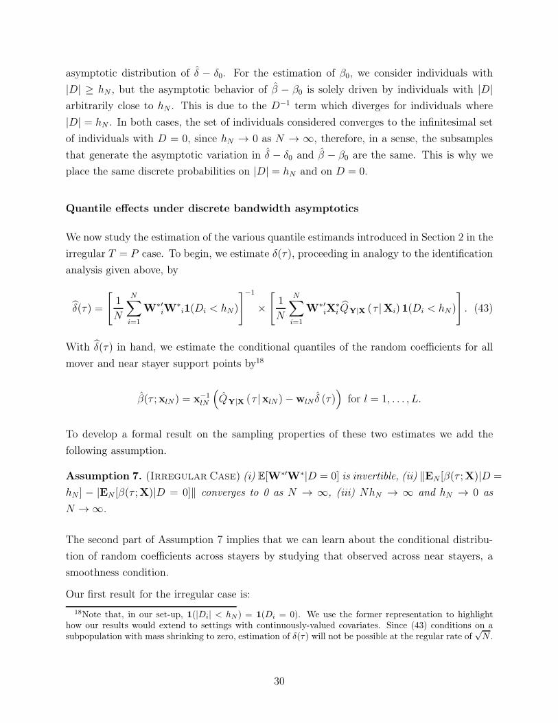
asymptotic distribution of δ − δ0. For the estimation of β0, we consider individuals with
|D| ≥ hN , but the asymptotic behavior of β − β0 is solely driven by individuals with |D|arbitrarily close to hN . This is due to the D−1 term which diverges for individuals where
|D| = hN . In both cases, the set of individuals considered converges to the infinitesimal set
of individuals with D = 0, since hN → 0 as N → ∞, therefore, in a sense, the subsamples
that generate the asymptotic variation in δ − δ0 and β − β0 are the same. This is why we
place the same discrete probabilities on |D| = hN and on D = 0.
Quantile effects under discrete bandwidth asymptotics
We now study the estimation of the various quantile estimands introduced in Section 2 in the
irregular T = P case. To begin, we estimate δ(τ), proceeding in analogy to the identification
analysis given above, by
δ(τ) =
[1
N
N∑
i=1
W∗′iW
∗i1(Di < hN)
]−1
×[1
N
N∑
i=1
W∗′iX
∗i QY|X (τ |Xi) 1(Di < hN )
]. (43)
With δ(τ) in hand, we estimate the conditional quantiles of the random coefficients for all
mover and near stayer support points by18
β(τ ;xlN ) = x−1lN
(QY|X (τ |xlN )−wlN δ (τ)
)for l = 1, . . . , L.
To develop a formal result on the sampling properties of these two estimates we add the
following assumption.
Assumption 7. (Irregular Case) (i) E[W∗′W
∗|D = 0] is invertible, (ii) ‖EN [β(τ ;X)|D =
hN ] − |EN [β(τ ;X)|D = 0]‖ converges to 0 as N → ∞, (iii) NhN → ∞ and hN → 0 as
N → ∞.
The second part of Assumption 7 implies that we can learn about the conditional distribu-
tion of random coefficients across stayers by studying that observed across near stayers, a
smoothness condition.
Our first result for the irregular case is:
18Note that, in our set-up, 1(|Di| < hN ) = 1(Di = 0). We use the former representation to highlighthow our results would extend to settings with continuously-valued covariates. Since (43) conditions on asubpopulation with mass shrinking to zero, estimation of δ(τ) will not be possible at the regular rate of
√N .
30
Theorem 5. Suppose that Assumptions 1 through 5 and 7 are satisfied, then under the
discrete bandwidth framework
(i)√NhN
(δ (·)− δ (·)
)converges in distribution to a mean zero Gaussian process Zδ (·),
where Zδ (·) is defined by its covariance function
Σδ(τ, τ′) = E[Zδ (τ)Zδ (τ
′)′]
=(min(τ, τ ′)− ττ ′)
2φ0E[W
∗′W
∗|D = 0]−1×
E[W
∗′X
∗Λ(τ, τ ′;X)X∗′W
∗|D = 0]E[W
∗′W
∗|D = 0]−1
, (44)
(ii)√NhN
(β (·;xlN)− β (·;xlN)
)also converges in distribution for each l = 1, . . . , L1 to a
mean zero Gaussian process Z (·,xl), where Z (·,xl) is defined by its covariance function
Σ(τ,xl, τ′,xm) = E
[Z (τ,xl)Z (τ ′,xm)
′]= x
−1l wlΣδ(τ, τ
′)w′mx
−1′m (45)
for l, m = 1, . . . , L1 and
(iii)√Nh3N
(β (·;xlN)− β (·;xlN)
)also converges in distribution for each l = L1 +1, . . . , L
to a mean zero Gaussian process Z (·,xl), where Z (·,xl) is defined by its covariance function
Σ(τ,xl, τ′,xm) = E
[Z (τ,xl)Z (τ ′,xm)
′](46)
= (min (τ, τ ′)− ττ ′)x∗lΛ (τ, τ ′;xl)x
∗′l
ql|02φ0
· 1 (l = m)
+w∗lΣδ(τ, τ
′)w∗′m
for l, m = L1 + 1, . . . , L.
Proof. See Appendix B.
The rate of convergence for δ(τ) coincide with that which would be expected when X has
a continuous distribution, as in Graham and Powell (2012). The δ(τ) estimator relies on
the sample with D = 0, which has fraction equal to 2φ0hN giving an effective sample size
of approximately 2Nφ0hN for estimation. As φ0 increases, more effective observations are
available for estimation, and therefore the asymptotic precision increases. The influence of
the preliminary quantile estimator appears through the Λ(τ, τ ′;X) matrix.
The conditional coefficient estimates, β (τ ;xlN), converge at different rates depending on
whether xlN has shrinking mass or not. Since these estimates depend linearly on δ(τ), their
fastest possible rate of convergence is√NhN , the rate of convergence of δ(τ). This rate
31
is achieved for (strict) movers, whose population frequencies are bounded away from zero.
In fact, for movers, the only component of the asymptotic variance of β (τ ;xlN) is due to
sampling variability in δ(τ), since the other ingredient to the estimator, the conditional
quantiles of Yt, are estimated at rate√N .
For units whose covariate sequences have shrinking mass, that is, for near-stayers, the rate
of convergence of β (τ ;xlN) is√Nh3N . For near stayers, X−1 = X
∗D−1, which diverges since
D = hN → 0 as N → ∞. To account for, and cancel, this shrinking denominator term, the
extra hN term is present. Note that we do not require that Nh3N → ∞ as N → ∞, and
in fact these conditional betas will not be consistently estimated if Nh3N → 0. This is not
a problem, since their consistent estimation is not the goal. Rather, we will show that the
ACQE and UQE estimators can incorporate these inconsistent estimates and still deliver a
consistent and asymptotically normal estimator for these functionals.
We now turn to the estimation of the average conditional quantile effect (ACQE). The
ACQE is consistently estimable under our discrete bandwidth setup because the mass of
stayers shrinks to zero as N → ∞. Specifically, the ACQE is identified by the limit β(τ) =
limN→∞ EN
[β(τ ;X)|X ∈ XM
N
]since β(τ ;X) is identified on XM
N and the probability mass of
stayers vanishes as N goes to infinity. Our estimate of the ACQE in the T = P case is
βN (τ) =1N
∑Ni=1X
−1i
(QY|X (τ |Xi)−Wiδ(τ)
)1(Xi ∈ XM
N )
1N
∑Ni=1 1(Xi ∈ XM
N ).
Theorem 6. Under Assumptions 1 through 5, Assumption 7, and Nh3N → 0, we have that,
under the discrete bandwidth framework:
√NhN
(βN(τ)− βN(τ))
d→ Zβ(τ),
a zero mean Gaussian process, on τ ∈ (0, 1). The variance of the Gaussian process Zβ(·) is
defined as
E[Zβ(τ)Zβ(τ
′)′]= Υ1(τ, τ
′) + Ξ0Σδ(τ, τ′)Ξ′
0 (47)
with
Υ1(τ, τ′) = 2φ0 (min (τ, τ ′)− ττ ′)E [X∗Λ(τ, τ ′,X)X∗′|D = 0]
Ξ0 = limN→∞
EN
[X
−1W| |D| ≥ hN
].
Proof. See Appendix B.
32
The rate of convergence of βN(τ) is√NhN , as is the case for the average effect studied by
Graham and Powell (2012). The asymptotic variance depends only on terms with D = 0,
since only stayers and near stayers contribute to the asymptotic distribution of the estimator.
If φ0 increases, it is possible to estimate the term Ξ0Σδ(τ, τ′)Ξ′
0 with more precision since
δ(τ) is more precisely determined when there are many units with D = 0. On the other
hand, term Υ1(τ, τ′) increases with φ0. The intuition behind this increase is that there are
more near-stayers when φ0 is large, and their contributions to βN(τ) are estimated at a
slower rate than those of movers.
Finally we turn to the unconditional quantile effect, βp(τ), the τ th quantile of Bp. As in the
regular case our estimate is the solution to (36). The only difference between the regular
and irregular case is the method used to estimate the conditional quantile effects βp(τ,x).
Theorem 7. Fix p ∈ {1, . . . , P}. Under the assumptions maintained in Theorem 6 we have
that
√NhN
(βp(τ)− βp(τ)
)d→ Zβp(τ)
on τ ∈ (0, 1) with Zβp(·) being a zero mean Gaussian process. The covariance of this Gaussian
process is equal to:
E[Zβp(τ)Zβp(τ
′)′]=
Υ3(τ, τ′) + Υ4(τ, τ
′)
fBp(βp(τ))fBp
(βp(τ ′))
where
Υ3(τ, τ′) = 2φ0E
[e′pX
−1Λ(FBp|X(βp(τ)|X), FBp|X(βp(τ′)|X),X)X−1′ep
× (min(FBp|X(βp(τ)|X), FBp|X(βp(τ′)|X))− FBp|X(βp(τ)|X)FBp|X(βp(τ
′)|X))
×fBp|X(βp(τ)|X)fBp|X(βp(τ′)|X)|D = 0
]
Υ4(τ, τ′) =
L∑
l=1
L∑
l′=1
e′p(x−1l wlpl1(l ≤ L1)
+w∗l ql|02φ01(l > L1))Σδ(FBp|X(βp(τ)|xl), FBp|X(βp(τ
′)|Xl′))
× (x−1l′ wl′pl′1(l
′ ≤ L1) +w∗l′ql′|02φ01(l
′ > L1))′epfBp|X(βp(τ)|xl)fBp|X(βp(τ
′)|xl′).
Proof. See Appendix B.
The asymptotic distribution of the UQE depends on the conditional density of Bp|X evalu-
ated at βp(τ). The term Υ3(·) reflects the estimation error for the near-stayers’ conditional
33
quantile effects. The overall rate of convergence is (NhN )−1/2. Although the conditional
quantile effects of near stayers converge at rate (Nh3N )−1/2 , they enter the UQE with a
weight which is of order O(hN), leading to the (NhN)−1/2 rate. The Υ4(·) term reflects
the influence of estimation error in δ(τ). Both these terms are divided by the density of
Bp evaluated at βp(τ), meaning that a larger density of the random coefficient around the
estimated quantile will lead to a smaller asymptotic variance. How the constant φ0 enters
these equation tells us that a smaller density of stayers and near-stayers will lead to smaller
asymptotic contribution of term Υ3(·) since there are less stayers excluded from the UQE
estimator. On the other hand, a lower φ0 can increase Υ4(·) since it reduces the precision of
the estimator of δ(τ), due to a lower relative sample size.
4 Union wage premium
The effect of collective bargaining coverage on the distribution of earnings is a question of
longstanding interest to labor economists (e.g., Card, Lemieux and Riddell, 2004). This is
also an area where both panel data and quantile regression methods have played important
roles in empirical work (e.g., Chamberlain, 1982; Jakubson, 1991; Card, 1995; Chamberlain,
1994), making an analysis which combines both approaches of particular interest.
We begin with a target sample consisting of the 4,837 male NLSY79 respondents in the cross-
sectional and supplemental Black and Hispanic subsamples. Our frame excludes respondents
in the supplementary samples of poor whites and military personnel (cf., MaCurdy, Mroz
and Gritz, 1998). We constructed a balanced panel of respondents who were (i) engaged
in paid private sector or government employment in each of the years 1988 to 1992 and (ii)
had complete wage and union coverage information. Exclusion from the estimation sample
occurred for several reasons. We excluded all self-employed individuals, individuals with
stated hourly wages less than $1, or greater than $1,000, in 2010 prices, and individuals who
were not surveyed in all five calendar years. We use the hourly wage measure associated with
each respondent’s “CPS” job. Our measure of collective bargaining coverage is also defined
vis-a-vis the CPS job.19 Respondents were between the ages of 24 and 33 in 1988 and hence
past the normal school-leaving age.
Our estimation sample is similar to that used by Chernozhukov, Fernandez-Val, Hahn and
Newey (2013), who also study the union wage premia using the NLSY79. Our subsample
19The “CPS” job coincides with a respondents primary employment as determined by the same criteriaused in the Current Population Survey (CPS).
34

Table 1: Union wage premiumFull Stayers Movers
Sample Never Always
Black (N=2,444) 0.1168 0.0864 0.1510 0.1868
Hispanic (N=2,444) 0.0602 0.0568 0.0616 0.0692
Years of Schooling (N=2,437)12.99(2.17)
13.24(2.31)
12.59(1.50)
12.50(1.92)
AFQT percentile (N=2,351)52.00(29.88)
56.57(29.91)
47.72(25.86)
40.87(28.34)
Source: National Longitudinal Survey of Youth 1979 and authors’ calculations.
Notes: Analysis based of the balanced panel of NLSY79 2,444 male respondents (in 2,104 households)
described in the main text. AFQT corresponds to Armed Force Qualification Test. Stayers consist of
workers who are never covered by a collective bargaining agreement as well as those who are always covered.
Movers consist of individuals who move in and/or out of coverage during the sample period. Sample sizes
are smaller for some covariates due to item non-response.
includes slightly more individuals, primarily by virtue of the fact that we follow respondents
for five instead of eight years, reducing attrition.
Table 1 reports a selection of worker attributes known to be predictive of wages by collec-
tive bargaining coverage status. Column 1 reports the mean of these characteristics across
all individuals in our sample (standard deviations are in parentheses for non-binary-valued
variables). Column 2 reports the corresponding statistics for workers who are never covered
by a collective bargaining agreement during the sample period, column 3 for those who are
always covered, and column 4 for those who mover in and/or out of coverage during the
sample period. Movers are more likely to be minority and have lower years of completed
school and AFQT scores. Workers who are never covered, have the lowest minority share,
the greatest years of completed schooling, and highest AFQT scores.
Table 2 reports out main results. All specifications allow for shifts in the intercept over time,
but maintain homogeneity of slope coefficients across time. Column 1 reports the coefficient
on the union dummy in a simple pooled least squares fit of log wages onto the union dummy
and a vector of year dummies. Column 2 reports the union coefficient in a specification
that additionally adds a vector of covariates for race, education and AFQT (see the notes to
Table (2) for details). Column 3 reports the union wage premium in a specification which
includes worker-specific intercepts. The estimator is as described by Arellano and Bover
(1995), which is a GMM variant of Chamberlain’s (1984) minimum distance estimator for
linear panel data models. Column 4 reports an estimate of the movers’ average union wage
premium using the variant of Chamberlain’s (1992) correlated random coefficients estimator
described in Graham and Powell (2012, Section 3.3). The movers average union effect is
between one-half and two-thirds of the OLS estimates of Columns 1 and 2. It is also very
35
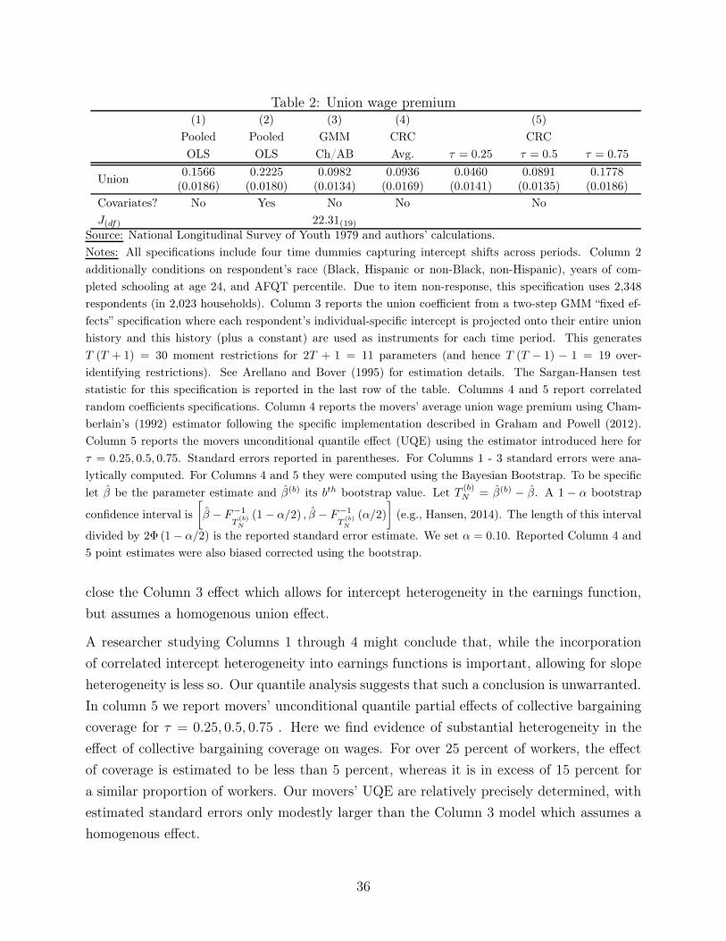
Table 2: Union wage premium(1) (2) (3) (4) (5)
Pooled Pooled GMM CRC CRC
OLS OLS Ch/AB Avg. τ = 0.25 τ = 0.5 τ = 0.75
Union0.1566(0.0186)
0.2225(0.0180)
0.0982(0.0134)
0.0936(0.0169)
0.0460(0.0141)
0.0891(0.0135)
0.1778(0.0186)
Covariates? No Yes No No No
J(df) 22.31(19)Source: National Longitudinal Survey of Youth 1979 and authors’ calculations.
Notes: All specifications include four time dummies capturing intercept shifts across periods. Column 2
additionally conditions on respondent’s race (Black, Hispanic or non-Black, non-Hispanic), years of com-
pleted schooling at age 24, and AFQT percentile. Due to item non-response, this specification uses 2,348
respondents (in 2,023 households). Column 3 reports the union coefficient from a two-step GMM “fixed ef-
fects” specification where each respondent’s individual-specific intercept is projected onto their entire union
history and this history (plus a constant) are used as instruments for each time period. This generates
T (T + 1) = 30 moment restrictions for 2T + 1 = 11 parameters (and hence T (T − 1) − 1 = 19 over-
identifying restrictions). See Arellano and Bover (1995) for estimation details. The Sargan-Hansen test
statistic for this specification is reported in the last row of the table. Columns 4 and 5 report correlated
random coefficients specifications. Column 4 reports the movers’ average union wage premium using Cham-
berlain’s (1992) estimator following the specific implementation described in Graham and Powell (2012).
Column 5 reports the movers unconditional quantile effect (UQE) using the estimator introduced here for
τ = 0.25, 0.5, 0.75. Standard errors reported in parentheses. For Columns 1 - 3 standard errors were ana-
lytically computed. For Columns 4 and 5 they were computed using the Bayesian Bootstrap. To be specific
let β be the parameter estimate and β(b) its bth bootstrap value. Let T(b)N = β(b) − β. A 1 − α bootstrap
confidence interval is
[β − F−1
T(b)N
(1− α/2) , β − F−1
T(b)N
(α/2)
](e.g., Hansen, 2014). The length of this interval
divided by 2Φ (1− α/2) is the reported standard error estimate. We set α = 0.10. Reported Column 4 and
5 point estimates were also biased corrected using the bootstrap.
close the Column 3 effect which allows for intercept heterogeneity in the earnings function,
but assumes a homogenous union effect.
A researcher studying Columns 1 through 4 might conclude that, while the incorporation
of correlated intercept heterogeneity into earnings functions is important, allowing for slope
heterogeneity is less so. Our quantile analysis suggests that such a conclusion is unwarranted.
In column 5 we report movers’ unconditional quantile partial effects of collective bargaining
coverage for τ = 0.25, 0.5, 0.75 . Here we find evidence of substantial heterogeneity in the
effect of collective bargaining coverage on wages. For over 25 percent of workers, the effect
of coverage is estimated to be less than 5 percent, whereas it is in excess of 15 percent for
a similar proportion of workers. Our movers’ UQE are relatively precisely determined, with
estimated standard errors only modestly larger than the Column 3 model which assumes a
homogenous effect.
36
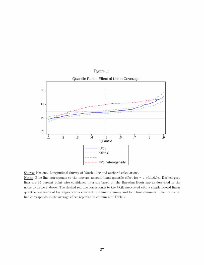
Figure 1:
−.2
0.2
.4
.1 .2 .3 .4 .5 .6 .7 .8 .9Quantile
UQE95% CI
w/o heterogeneity
Quantile Partial Effect of Union Coverage
Source: National Longitudinal Survey of Youth 1979 and authors’ calculations.
Notes: Blue line corresponds to the movers’ unconditional quantile effect for τ ∈ (0.1, 0.9). Dashed grey
lines are 95 percent point wise confidence intervals based on the Bayesian Bootstrap as described in the
notes to Table 2 above. The dashed red line corresponds to the UQE associated with a simple pooled linear
quantile regression of log wages onto a constant, the union dummy and four time dummies. The horizontal
line corresponds to the average effect reported in column 4 of Table 2
37
Figure 1 plots our estimated movers’ unconditional quantile effects as well as 95 percent
point-wise confidence bands. The figure also includes quantile effects associated with a
model which does not incorporate correlated heterogeneity. These effects are estimated by a
linear quantile regression of wages onto a constant, the union dummy and four time dummies.
The coefficients on the union dummy, rearranged to be monotonic, are plotted as the dashed
red line. As is the case for mean effects, quantile partial effects of union coverage are severely
overstated in models which do not allow unobserved worker attributes to covary with union
status.
Our empirical analysis also allows for assessment of the impact of collective bargaining
coverage on inequality, at least within the subpopulation of movers. The counterfactual
1992 average 90-10 log wage gap in a world with no collective bargaining coverage is given
by
E
[(1
0
)′
([β (0.9;X) + δ92 (0.9)]− [β (0.1;X) + δ92 (0.9)])
∣∣∣∣∣X ∈ XM
].
The corresponding gap in a world of universal coverage is given by
E
[(1
1
)′
([β (0.9;X) + δ92 (0.9)]− [β (0.1;X) + δ92 (0.9)])
∣∣∣∣∣X ∈ XM
].
We estimate an average 90-10 gap in the no coverage counterfactual of 1.28. The corre-
sponding gap in the universal coverage case is 1.07. The difference is 0.22 with a standard
error of 0.08. Our analysis implies that unions have a substantially compressing effect on
the distribution of wages, at least within the movers subpopulation.
5 Extensions
Using stayers to identify time effects when T > P
When identification is regular, as outlined above, δ (τ) is estimable using mover units alone.
However, it may nevertheless be advantageous to incorporate stayer units into the estimation
procedure. This can improve the precision of δ (τ). It can also increase the precision with
which the movers’ ACQE and UQE are estimated, through the influence of sampling error
in δ (τ) on the asymptotic variance of both of these objects (see Theorems 3 and 4 above).
Let xl denote a stayer realization of X and consider the full rank decomposition xl = ulvl.
Let mul= IT − ul (u
′lul)
−1ul and observe that mul
x = ulvl − ul (u′lul)
−1ulvl = 0. We
38
therefore have
mulQY|X (τ |x) = mul
wδ (τ)
for l = L+1, . . . ,M . If we define Π (τ) =(Π (τ)′ ,muL+1
QY|X (τ |x)′ , . . . ,muMQY|X (τ |x)′
)′
and G = (G′, (G∗)′)′, with G as defined in (29) and G∗ equal to
G∗
T (M−L)×(R+PL)=
muL+1w 0T0
′P · · · 0T0
′P
......
. . ....
muMw 0T0
′P · · · 0T0
′P
,
we have the relationship Π (τ) = Gγ (τ), upon which the obvious analog estimator may be
based. In fact we incorporate stayers in this way in the empirical analysis reported in Section
4.
Non-shrinking mass of stayers in the irregular case
In some applications, it is common to observe a positive mass of stayers at D = 0 along with
a small number of near-stayers. We can model this in our discrete bandwidth framework by
letting Pr(D = 0) = π0 + 2φ0hN where π0 > 0 and keeping Pr(D = hN ) = Pr(D = −hN) =φ0hN .
In this case, it will be possible to estimate δ(τ) at a√N rate since the mass of stayers is
bounded away from 0. On the other hand, the conditional beta for near-stayer realizations
will still be estimated at rate√Nh3N since the slowest rate of convergence prevails. Their
asymptotic variance will be reduced since the term associated with the estimation of δ(τ)
vanishes. Estimation of conditional betas for strict-mover realizations can now be performed
at the√N rate rather than
√NhN .
Despite these improvements, the movers’ ACQE now becomes inconsistent since the fraction
of stayers does not vanish asymptotically. We can modify the estimator and include the
near-stayers’ coefficients as an approximation to the stayers’ coefficients in the following
way:
ˆβN (τ) =
L∑
l=1
β(τ ;xlN)qMlN
{1
N
N∑
i=1
1(Di 6= 0)
}+
L∑
l=L1+1
β(τ ;xlN)ql|±h
{1
N
N∑
i=1
1(Di = 0)
},
where ql|±h =1
N
∑Ni=1
1(Xi=xlN )1
N
∑Ni=1
1(|Di|=hN ). The term
∑Ll=L1+1 β(τ ;xlN)ql|±h approximates E[β(τ ;X)|X ∈
39
XSN ] using the near-stayers. The conditional beta for near-stayers is estimated at rate
√Nh3N
but their contribution is now of order Op(1) rather than Op(hN) in the previous case. There-
fore, the convergence rate of the ACQE estimator will be√Nh3N as well.
The same concern applies in the UQE estimation where the share of stayers does not vanish
asymptotically. It is also possible to show that the rate of convergence will deteriorate
from√NhN to
√Nh3N . The result in this case is analogous to that in Graham and Powell
(2012) where the mass at D = 0 simplifies the estimation of the common coefficients while
complicating the estimation of average partial effects.
In the case when there is a mass of stayers but no near-stayers, i.e. Pr(D = 0) = π0 and
Pr(|D| = hN) = 0, it is not possible to identify the ACQE and UQE. This is a result similar
to that found in the overidentified case, which does not contain near-stayers as well. Rates of
convergence for the movers’ ACQE and the movers’ UQE will be of order N−1/2, since there
is no shrinking mass of near-stayers involved in the rate calculations. It is also possible to
show the set identification of the ACQE and the UQE in a way similar to the overidentified
case. We present the results for the just-identified case with no near-stayers in detail in
Appendix A.
Continuous regressors
The identification results in the previous section are all based on the conditional quantiles
of Yt given X = x for t = 1, . . . , T . There are different methods of estimating these condi-
tional quantiles depending on the structure of the support of X. When the support of X
is discrete, as is assumed in this paper, we can write by standard arguments the following
linear representation of our first step conditional quantile estimator:
QYt|X (τ |x)−QYt|X (τ |x) = 1
N
N∑
i=1
(1(Yit ≤ QYt|X(τ |x)
)− τ)1(Xi = x)
fYt|X(QYt|X(τ |x)|x)pN+ RN(τ ;x) (48)
where pN is the probability associated with support point x and the residual RN(τ ;x) goes
to 0 in probability as N → ∞.
A kernel based estimator can be used to compute the analog estimator when X has continuous
support. Examples include local linear regression (Qu and Yoon, forthcoming), or inversion
of conditional CDF estimates (Lee, 2013). The Bahadur representation of these estimators
40

is the following:
QYt|X (τ |x)−QYt|X (τ |x)
=1
NbTP
N∑
i=1
(1(Yit ≤ QYt|X(τ |x)
)− τ)K (B−1 (vec(Xi)− vec(x)))
fYt|X(QYt|X(τ |x)|x)fX(x)+RN(τ ;x) (49)
where K(·) is a kernel function, and B = bITP where b is a bandwidth converging to 0.
These representations contain just two differences. The first difference is the presence of the
kernel in the continuous case. We note that this kernel function converges to an indicator
for {Xi = x} whenever K(0) = 1. This restriction is satisfied by different kernels, including
a uniform kernel with support [−1/2, 1/2].
The second difference is the density of X versus its probability that it is equal to x. The
bandwidth term bTP also is present with the density. These two terms can be reconciled
if we consider the probability that X is included in a TP -dimensional neighborhood of x
with diameter equal to b. For exposition, consider T = P = 1. Then, the probability
that X ∈ [x − b/2, x + b/2] is approximately equal to fX(x)b. This probability can be
approximated with the mass pN if this mass depends on the sample size through b such that
pN = O(b). That way, discrete probabilities will behave like probabilities for continuous
densities, and NpN will be the approximate sample size for the support point, similar to the
Nb in traditional nonparametric density estimation.
We see that there is no substantial difference between the asymptotic representations, except
that it is much simpler to impose conditions on the asymptotic convergence of Πt (τ ;x) −Πt (τ ;x) in the discrete case than in the continuous case. For this reason, we conjecture
that our rates of convergence and limit distribution results will generalize to the case of
continuous regressors (under additional regularity conditions). Such an extension, however,
is likely to be difficult and non-trivial.
Choice of Bandwidth
In this spirit of the argument given immediately above, we can use our discrete bandwidth
asymptotics to gain some insight into bandwidth selection. As discussed earlier, we need that
hN → 0, NhN → ∞, and Nh3N → 0 as N → ∞. These conditions allow us to put shrinking
mass on some support points (hN → 0), while allowing for consistent estimation of objects
conditional on these shrinking mass support points (NhN → ∞). The third condition is
required to eliminate the bias in our estimators for the ACQE and UQE. Let a be a P × 1
vector of constants. The fastest rate of convergence in mean square for either a′ ˆβ(τ) to
41

a′β(τ) or βp(τ) to βp(τ) is N−2/3 with bandwidth sequences of the form h∗N = C0N−1/3 for
some constant C0. Consider first the MSE for the estimator a′ ˆβ(τ). Using the results of
Theorem 6, the asymptotic bias will be equal to
bias = 2a′(E[β(τ ;X)]− E[β(τ ;X)|D = 0])φ0hN
and therefore the asymptotic MSE minimizing bandwidth constant is
C0 =1
2
(1
φ20
)1/3(a′ (Υ1(τ, τ) + Ξ0Σδ(τ, τ)Ξ
′0) a
a′(E[β(τ ;X)]− E[β(τ ;X)|D = 0])(E[β(τ ;X)]− E[β(τ ;X)|D = 0])′a
)1/3
which is similar to the one found in Graham and Powell (2012) for average partial effects.
Since choosing bandwidth with order exactly equal to N−1/3 leads to an asymptotic bias,
we can choose a slightly faster bandwidth sequence, say, of order o(N−1/3) such that the
asymptotic bias disappears. An alternative is to use a plug-in bandwidth using an estimate
of C0 and then bias correct. This approach preserves the rate of convergence of N−1/3.
We now consider the bias associated with the estimation of βp(τ), the UQE associated with
the pth regressor. The leading term of the asymptotic bias of βp(τ) is equal to
bias = 2φ0hNFBp
(βp(τ))− FBp|D=0(βp(τ))
fBp(βp(τ))
.
Once again, the MSE minimizing rate for the bandwidth is N−1/3 and the mean squared
error minimizing choice of constant is
C0 =1
2
(1
φ20
)1/3(
Υ3(τ, τ) + Υ4(τ, τ)[FBp
(βp(τ))− FBp|D=0(βp(τ))]2
)1/3
.
Trimming Extremal Quantiles
Estimation of quantiles can become problematic when the quantile considered is close to 0 or
1. As an example, the estimation of unconditional quantiles of a scalar random variable does
not converge in process over τ ∈ (0, 1) when the support of the random variable is unbounded.
On the other hand, it does converge when considering τ ∈ [ǫ, 1 − ǫ] for any 0 < ǫ < 1/2.
Whether the support is bounded or not, trimming extremal quantiles is common practice
since estimators for them may be poorly approximated by the same asymptotic distribution
as non-extremal quantiles. This could lead to a problem for the identification of β(τ) since
42

it requires the use of β(τ ;X) for all τ ∈ (0, 1). Trimming any fixed amount of quantiles will
result in a loss of point identification.
Suppose that the researcher proceeds with the estimation of conditional quantiles ranging
from τ = ǫ to τ = 1 − ǫ so that only these conditional quantiles are identified. We can
decompose the moment condition used for the estimation of βp(τ) for p = 1, . . . , P in three
parts:
τ = m(b)
= E
[ˆ 1
0
1(βp(u;X) ≤ b)du
]
= E
[ˆ ǫ
0
1(βp(u;X) ≤ b)du
]+ E
[ˆ 1−ǫ
ǫ
1(βp(u;X) ≤ b)du
]+ E
[ˆ 1
1−ǫ
1(βp(u;X) ≤ b)du
].
The first and third term are uniformly bounded below and above by 0 and ǫ respectively.
Therefore,
τ − 2ǫ ≤ E
[ˆ 1−ǫ
ǫ
1(βp(u;X) ≤ b)du
]≤ τ.
Let V be uniformly distributed on [ǫ, 1 − ǫ] independently from X. We can think of this V
as the trimmed version of the unobserved heterogeneity U . Then, we see that
τ − 2ǫ
1− 2ǫ≤ Fβp(V ;X)(b) ≤
τ
1− 2ǫ,
and therefore, the UQE for the pth regressor is partially identified with bounds equal to
βp(τ) ∈[F−1βp(V ;X)
(τ − 2ǫ
1− 2ǫ
), F−1
βp(V ;X)
(τ
1− 2ǫ
)].
These lower and upper bounds are identified since we can identify β(τ ;X) when τ ∈ [ǫ, 1−ǫ].We also see that this identification region collapses to a point as ǫ approaches zero. These
bounds may be used instead of the point estimates if it is believed that a significant portion
of the conditional quantiles need to be trimmed. The researcher may also compare the lower
and upper bounds’ estimates to get a rough sense of the contribution of these extremal
quantiles to identification.
43

6 Conclusion
The extension of quantile regression methods to panel data has proved to be especially
challenging due to the non-linearity of quantiles. Our approach to this challenge generalizes
both the textbook linear quantile regression and linear panel data models. Relative to these
benchmarks our set-up allows for richer types of correlated (unobserved) heterogeneity, while
still offering positive identification results. While the large sample theory of our estimators
is non-trivial, their computation is not, requiring only sorting and weighted least squares
operations. Our empirical analysis illustrates some of the possibilities of our approach.
One area of application where our methods may be especially attractive to researchers is for
program and policy evaluation. As a concrete example consider a researcher who wishes to
study the effect of minimum wage laws on the distribution of earnings using several waves of
the Current Population Survey (CPS). Here X would encode the minimum wage level over
time within a state. Since we observe many workers per state in each period, and hence
per realization of X, our discrete covariate results apply. Specifically FYt|X (y|x) may be
estimated by the empirical distribution function of period t wages in states with minimum
wage sequence X = x. Applications in educational policy, where the entire distribution of
test scores may be of interest, are also natural.
Our paper is not the first to explore the intersection of quantile regression and panel data.
Here we briefly touch on the relationship between our work and two very recent contributions.
Chernozhukov, Fernandez-Val, Hahn and Newey (2013), CFHN for short, includes some
results on quantile effects in the context of a wide-ranging analysis of identification in non-
separable panel data models. The simplest case allowing for interesting comparisons between
their results and our own is when P = 2 with the non-constant covariate binary-valued (i.e.,
Xt = (1, X2t)′ with X2t ∈ {0, 1}). For simplicity we ignore time effects in what follows so
that the conditional distribution of Yt given X = x is stationary over time and, if (3) is also
being maintained, so is the distribution of random coefficients.
Following the notation of CFHN let Ti (x) =∑T
t=1 1 (Xit = x) and define
Gi (y, x) =
{Ti (x)
−1∑Tt=1 1 (Xit = x) 1 (Yit ≤ y) , Ti (x) > 0
0, Ti (x) = 0
and also
GM (y, x) =
∑Ni=1 Gi (y, x)1
(Xi ∈ XM
)∑N
i=1 1 (Xi ∈ XM).
44
Their quantile treatment effect (QTE) estimate is
λ (τ) = G−1M (τ, 1)− G−1
M (τ, 0) .
To understand the relationship between λ (τ) and our unconditional quantile effect (UQE)
estimand further, we simplify to the case where T = 2. Let
π01 = Pr(X21 = 0, X22 = 1|X ∈ XM
)and π10 = Pr
(X21 = 1, X22 = 0|X ∈ XM
). Let
GM (y, x)p→ GM (y, x), under the random coefficients data generating process (3) we have
that
GM (y, 1) = π01FB1+B2
(y|X22 = 1,X ∈ X
M)+ π10FB1+B2
(y|X21 = 1,X ∈ X
M)
GM (y, 0) = π01FB1
(y|X21 = 0,X ∈ X
M)+ π10FB1
(y|X22 = 0,X ∈ X
M),
so that λ (τ) = G−1M (τ, 1)−G−1
M (τ, 0) does not correspond to any quantile of B2, even if
our conditional monotonicity assumption holds. Indeed if we set
FB1+B2
(y|X22 = 1,X ∈ XM
)= FB1
(y|X22 = 0,X ∈ XM
)and
FB1+B2
(y|X21 = 1,X ∈ XM
)= FB1
(y|X21 = 0,X ∈ XM
)for all y ∈ Yt we will have λ (τ)
identically equal to zero for all τ ∈ (0, 1) and our movers’ UQE, βM2 (τ), possibly different
from zero for all τ ∈ (0, 1). The difference between CFHN’s estimand and our movers’
UQE arises from how marginalization over X occurs. CFHN marginalize over X before
inverting to recover quantile effects, we first recover quantile effects for each possible
x ∈ XM and then ‘marginalize’. Under our correlated random coefficients structure the
CFHN estimand will, in general, not recover quantiles of B2.
Arellano and Bonhomme (2013) study identification and estimation of the model
QYt|X,A (τ |X, A) = X ′tβ (τ) + Aγ (τ)
for all τ ∈ (0, 1) . Here A corresponds to an unobserved time-invariant regressor. Arel-
lano and Bonhomme (2013) also allow for a particular form of dependence between X
and A, hence their model is a correlated random effects one. If A were observed, then
θ (τ) =(β (τ)′ , γ (τ)
)′could be estimated by the τ th linear pooled quantile regression of Yt
onto Xt and A (here the pooling is across all periods of data t = 1, . . . , T ). This set-up
represents an alternative generalization of the linear panel model of Chamberlain (1984) to
the quantile regression setting. The Arellano and Bonhomme (2013) approach and ours are
non-nested. Their model effectively includes two-dimensional unobserved heterogeneity. The
first component of this heterogeneity vector is A, this component is allowed to covary with
45

X is a reasonably flexible way. The second component corresponds to the common factor
in the random coefficients on Xt and A. This component is independent of both X and A.
Hence input “returns” and input choices are independent in their model. Relatedly their
set-up also requires a comonotonicity assumption on the random coefficients.
Our model, effectively, includes only a single dimension of unobserved heterogeneity. However
we impose weaker comonotonicity assumptions and leave the dependence structure between
the random coefficients and X nonparametric, allowing input ‘returns’ and input choices to
correlate. Our view is that both approaches are attractive, with the merits of each being
context specific.
References
[1] Abrevaya, Jason. (2001). “The effects of demographics and maternal behavior on the
distribution of birth outcomes,” Empirical Economics 26 (1): 247 - 257.
[2] Abrevaya, Jason and Christian M. Dahl. (2008). “The effects of birth inputs on birth-
weight,” Journal of Business & Economic Statistics 26 (4): 379 - 397.
[3] Angrist, Joshua, Victor Chernozhukov, and Iván Fernández-Val. (2006). “Quantile re-
gression under misspecification, with an application to the U.S. wage structure,” Econo-
metrica 74 (2): 539 - 563.
[4] Arellano, Manuel and Stéphane Bonhomme. (2011). “Nonlinear panel data analysis,”
Annual Review of Economics 3: 395 - 424.
[5] Arellano, Manuel and Stéphane Bonhomme. (2012). “Identifying Distributional Char-
acteristics in Random Coefficients Panel Data Models,” Review of Economic Studies 79
(3): 987 - 1020.
[6] Arellano, Manuel and Stéphane Bonhomme. (2013). “Random-effects quantile regres-
sions,” Mimeo, CEMFI.
[7] Arellano, Manuel and Olympia Bover. (1995). “Another look at the instrumental variable
estimation of error-components models,” Journal of Econometrics 68 (1): 29 - 51.
[8] Athey, Susan and Guido W. Imbens. (2006). “Identification and inference in nonlinear
difference-in-differences models,” Econometrica 74 (2): 431 - 497.
46

[9] Autor David H. ,Lawrence F. Katz and Melissa S. Kearney. (2008). “Trends in U.S.
wage inequality: revising the revisionists,” Review of Economics and Statistics 90 (2):
300 - 323.
[10] Bajari, Patrick, Jinyong Hahn, Han Hong and Geert Ridder. (2011). “A note on semi-
parametric estimation of finite mixtures of discrete choice models with applications to
game theoretic models,” International Economic Review 52 (3): 807 - 824.
[11] Buchinsky, Moshe. (1994). “Changes in the U.S. wage structure 1963-1987: application
of quantile regression,” Econometrica 62 (2): 405 - 458.
[12] Card, David. (1995). “The effects of unions on the structure of wages: a longitudinal
analysis,” Econometrica 64 (4): 957 - 979.
[13] Card, David, Thomas Lemieux and W. Craig Riddell. (2004). “Unions and wage in-
equality,” Journal of Labor Research 25 (4): 519 - 559.
[14] Chamberlain, Gary. (1982). “Multivariate regression models for panel data,” Journal of
Econometrics 18 (1): 5 - 46.
[15] Chamberlain, Gary. (1984). “Panel data,” Handbook of Economics 2: 1247 - 1318 (Z.
Griliches & M. Intriligator, Eds.). Amsterdam: North-Holland.
[16] Chamberlain, Gary. (1987). “Asymptotic efficiency in estimation with conditional mo-
ment restrictions,” Journal of Econometrics 34 (3): 305 - 334.
[17] Chamberlain, Gary. (1992). “Efficiency bounds for semiparametric regression,” Econo-
metrica 60 (3): 567 – 596.
[18] Chamberlain, Gary. (1994). “Quantile regression, censoring, and the structure of wages,”
Advances in Econometrics, Sixth World Congress I : 171 - 209. (C. Sims, Ed.). Cam-
bridge: Cambridge University Press.
[19] Chaudhuri, Probal, Kjell Doksum and Alexander Samarov. (1997). “On average deriva-
tive quantile regression,” Annals of Statistics 25 (2): 715 - 744.
[20] Chernozhukov, Victor, Ivan Fernández-Val and Alfred Galichon. (2010). “Quantile and
probability curves without crossing,” Econometrica 78 (3): 1093 - 1125.
[21] Chernozhukov, Victor, Ivan Fernandez-Val and Blaise Melly. (2013). “Inference on Coun-
terfactual Distributions,” Econometrica 81 (6): 2205 - 2268.
47
[22] Chernozhukov, Victor, Ivan Fernandez-Val, Jinyong Hahn and Whitney Newey. (2013).
“Average and quantile effects in nonseparable panel models,” Econometrica 81 (2): 535
- 580.
[23] Chernozhukov, Victor, Ivan Fernandez-Val, Stefan Hoderlein, Hajo Holzmann and
Whitney K. Newey. (2014). “Nonparametric identification in panels using quantiles,”
Mimeo.
[24] Chernozhukov, Victor and Christian Hansen. (2007). “Instrumental variable quantile
regression: a robust inference approach,” Journal of Econometrics 142 (1): 379 - 398.
[25] Clotilde, Elyès and Jouini Napp. (2004). “Conditional comonotonicity,” Decisions in
Economics and Finance 27 (2): 153 - 166.
[26] Firpo, Sergio. (2007). “Efficient semiparametric estimation of quantile treatment effects,”
Econometrica 75 (1): 259 – 276.
[27] Firpo, Sergio, Nicole M. Fortin and Thomas Lemieux. (2009). “Unconditional quantile
regressions,” Econometrica 77 (3): 953 – 973.
[28] Graham, Bryan S. and James L. Powell. (2012). "Identification and estimation of av-
erage partial effects in ‘irregular’ correlated random coefficient panel data models,"
Econometrica 80 (5): 2105 - 2152.
[29] Hahn, Jingyong and Whitney K. Newey. (2004). “Jackknife and analytical bias reduction
for nonlinear panel models,” Econometrica 72 (4): 1295 – 1319.
[30] Hansen, Bruce E. (2014). Econometrics. Mimeo, University of Wisconsin.
[31] Imbens, Guido. W. and Whitney K. Newey. (2009). “Identification and estimation of
triangular simultaneous equations models without additivity,” Econometrica 77 (5):
1481 – 1512.
[32] Jakubson, George. (1991). “Estimation and testing of the union wage effect using panel
data,” Review of Economic Studies 58 (5): 971 - 991.
[33] Kato, Kenjo, Antonio F. Galvao Jr., Gabriel V. Montes-Rojas. (2012). “Asymptotics for
panel quantile regression models with individual effects,” Journal of Econometrics 170
(1): 76 - 91.
[34] Khan, Shakeeb and Elie Tamer. (2010). “Irregular identification, support conditions,
and inverse weight estimation,” Econometrica 78 (6): 2021 – 2042.
48
[35] Kline, Patrick and Andres Santos. (2013). “Sensitivity to missing data assumptions:
Theory and an evaluation of the U.S. wage structure,” Quantitative Economics 4 (2):
231 – 267.
[36] Koenker, Roger. (2005). Quantile Regression. Cambridge: Cambridge University Press.
[37] Koenker, Roger and Gilbert Bassett, Jr. (1978). “Regression quantiles,” Econometrica
46 (1): 33 - 50.
[38] Lee, Ying-Ying. (2013). “Nonparametric weighted average quantile derivative,” Mimeo,
Nuffield College, Oxford University.
[39] Lemieux, Thomas. (2006). “Postsecondary education and increasing wage inequality,”
American Economic Review 96 (2): 195 - 199.
[40] Ma, Lingjie and Roger Koenker. (2006). “Quantile regression methods for recursive
structural equation models,” Journal of Econometrics 134 (2): 471 - 506.
[41] MaCurdy, Thomas, Thomas Mroz and R. Mark Gritz. (1998). “An evaluation of the
National Longitudinal Survey on Youth,” Journal of Human Resources 33 (2): 345 -
436.
[42] Machado, Jose. A. F. and Jose Mata. (2005). “Counterfactual decomposition of changes
in wage distributions using quantile regression,” Journal of Applied Econometrics 20
(4): 445 – 465.
[43] Manski, Charles F. (1987). “Semiparametric analysis of random effects linear models
from binary panel data,” Econometrica 55 (2): 357 - 362.
[44] Qu, Zhongjun and Jungmo Yoon. (forthcoming), “Nonparametric estimation and infer-
ence on conditional quantile processes,” Journal of Econometrics.
[45] Rosen, Adam. (2012). “Set identification via quantile restrictions in short panels,” Jour-
nal of Econometrics 166 (1):127 - 137.
[46] Vella, Francis and Marno Verbeek. (1998). “Whose wages do unions raise? A dynamic
model of unionism and wage rate determination for young men?” Journal of Applied
Econometrics 13 (2): 163 - 183.
[47] Wei, Ying and Raymond J. Carroll. (2009). “Quantile regression with measurement
error,” Journal of the American Statistical Association 104 (487): 1129 - 1143.
49
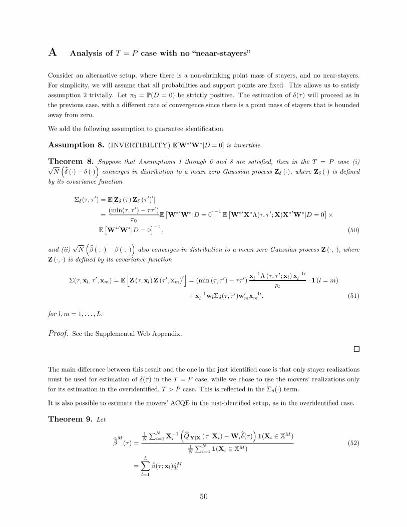
A Analysis of T = P case with no “neaar-stayers”
Consider an alternative setup, where there is a non-shrinking point mass of stayers, and no near-stayers.
For simplicity, we will assume that all probabilities and support points are fixed. This allows us to satisfy
assumption 2 trivially. Let π0 = P(D = 0) be strictly positive. The estimation of δ(τ) will proceed as in
the previous case, with a different rate of convergence since there is a point mass of stayers that is bounded
away from zero.
We add the following assumption to guarantee identification.
Assumption 8. (INVERTIBILITY) E[W∗′W
∗|D = 0] is invertible.
Theorem 8. Suppose that Assumptions 1 through 6 and 8 are satisfied, then in the T = P case (i)√N(δ (·)− δ (·)
)converges in distribution to a mean zero Gaussian process Zδ (·), where Zδ (·) is defined
by its covariance function
Σδ(τ, τ′) = E[Zδ (τ)Zδ (τ
′)′]
=(min(τ, τ ′)− ττ ′)
π0E[W
∗′W
∗|D = 0]−1
E[W
∗′X
∗Λ(τ, τ ′;X)X∗′W
∗|D = 0]×
E[W
∗′W
∗|D = 0]−1
, (50)
and (ii)√N(β (·; ·)− β (·; ·)
)also converges in distribution to a mean zero Gaussian process Z (·, ·), where
Z (·, ·) is defined by its covariance function
Σ(τ,xl, τ′,xm) = E
[Z (τ,xl)Z (τ ′,xm)
′]= (min (τ, τ ′)− ττ ′)
x−1l Λ (τ, τ ′;xl)x
−1′l
pl· 1 (l = m)
+ x−1l wlΣδ(τ, τ
′)w′mx
−1′m , (51)
for l,m = 1, . . . , L.
Proof. See the Supplemental Web Appendix.
The main difference between this result and the one in the just identified case is that only stayer realizations
must be used for estimation of δ(τ) in the T = P case, while we chose to use the movers’ realizations only
for its estimation in the overidentified, T > P case. This is reflected in the Σδ(·) term.
It is also possible to estimate the movers’ ACQE in the just-identified setup, as in the overidentified case.
Theorem 9. Let
βM
(τ) =
1N
∑Ni=1 X
−1i
(QY|X (τ |Xi)−Wiδ(τ)
)1(Xi ∈ XM )
1N
∑Ni=1 1(Xi ∈ XM )
(52)
=
L∑
l=1
β(τ ;xl)qMl
50
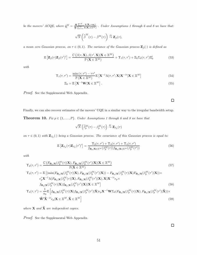
be the movers’ ACQE, where qMl =1N
∑Ni=1 1(Xi=xl)
1N
∑Ni=1 1(Xi∈XM )
. Under Assumptions 1 through 6 and 8 we have that:
√N
(βM
(τ)− βM (τ)
)D→ Zβ(τ),
a mean zero Gaussian process, on τ ∈ (0, 1). The variance of the Gaussian process Zβ(·) is defined as
E[Zβ(τ)Zβ(τ
′)′]=
C(β(τ,X), β(τ ′,X)|X ∈ XM
)
P (X ∈ XM )+ Υ1(τ, τ
′) + Ξ0Σδ(τ, τ′)Ξ′
0 (53)
with
Υ1(τ, τ′) =
min (τ, τ ′)− ττ ′
P (X ∈ XM )E[X
−1Λ(τ, τ ′;X)X−1′|X ∈ XM]
(54)
Ξ0 = E[X
−1W|X ∈ X
M]. (55)
Proof. See the Supplemental Web Appendix.
Finally, we can also recover estimates of the movers’ UQE in a similar way to the irregular bandwidth setup.
Theorem 10. Fix p ∈ {1, . . . , P}. Under Assumptions 1 through 6 and 8 we have that
√N(βMp (τ) − βM
p (τ))
D→ Zβp(τ)
on τ ∈ (0, 1) with Zβp(·) being a Gaussian process. The covariance of this Gaussian process is equal to:
E[Zβp
(τ)Zβp(τ ′)′
]=
Υ2(τ, τ′) + Υ3(τ, τ
′) + Υ4(τ, τ′)
fBp|X∈XM (βMp (τ))fBp|X∈XM (βM
p (τ ′))(56)
with
Υ2(τ, τ′) =
C(FBp|X(βM
p (τ)|X), FBp |X(βMp (τ ′)|X)|X ∈ XM
)
P(X ∈ XM )(57)
Υ3(τ, τ′) = E
[(min(FBp|X(βM
p (τ)|X), FBp |X(βMp (τ ′)|X))− FBp|X(βM
p (τ)|X)FBp |X(βMp (τ ′)|X))×
e′pX−1Λ(FBp|X(βM
p (τ)|X), FBp |X(βMp (τ ′)|X),X)X−1′ep×
fBp|X(βMp (τ)|X)fBp|X(βM
p (τ ′)|X)|X ∈ XM]
(58)
Υ4(τ, τ′) =
1
π0E
[fBp|X(βM
p (τ)|X)fBp |X(βMp (τ ′)|X)epX
−1WΣδ(FBp|X(βM
p (τ)|X), FBp |X(βMp (τ ′)|X))×
W′X
−1′ep|X ∈ XM , X ∈ X
M]
(59)
where X and X are independent copies.
Proof. See the Supplemental Web Appendix.
51

Since in this case the UQE is not point identified, we can recover bounds using the movers’ UQE as in
Theorem 1.
B Proofs of Theorems
Proof of Lemma 1
First consider the asymptotic distribution of the conditional CDF estimate
FYt|X(c|xmN ) =1N
∑Ni=1 1(Yit ≤ c,Xi = xmN )1N
∑Ni=1 1(Xi = xmN )
. (60)
We have that 1N
∑Ni=1 1(Xi = xmN ) − pmN = Op
(1√
NpmN
)and 1
N
∑Ni=1 1(Yit ≤ c,Xi = xmN ) − Pr(Yit ≤
c,X = xmN ) = Op
(1√
NpmN
). Using the delta method we get
FYt|X(c|xmN )− FYt|X(c|xmN ) =1
N
N∑
i=1
(1(Yit ≤ c,Xi = xmN )
pmN
− PN (Yt ≤ c|X = xmN )
pmN
1(Xi = xmN )
)
(61)
+Op
(1
NpmN
).
By Lyapunov’s Central Limit Theorem, and Assumptions 2 to 5, we have that, for fixed c, the normalized
difference√NpmN
(FYt|X(c|xmN )− FYt|X(c|xmN )
)is asymptotically normal with limiting variance equal
to
limN→∞
Pr(Yt ≤ c|X = xmN )(1 − Pr(Yt ≤ c|X = xmN ))
= Pr(Yt ≤ c|X = xm)(1 − Pr(Yt ≤ c|X = xm)).
Note that continuity of the conditional CDF of Yit given X, a component of Assumption 4, is important for
this result.
The next step is to show that the convergence of the normalized difference is uniform in c ∈ R and that
the limiting process is Gaussian. The normalized summand 1(Yit≤c,Xi=xmN )√pmN
− Pr(Yt≤c|X=xmN)√pmN
1(Xi = xmN )
can be shown to have a finite bracketing integral for any N (since indicator functions have finite bracketing
integrals) and Pr(Yt ≤ c|X = xmN ) has bounded derivatives in c since the conditional density of Yt given X
is uniformly bounded in all arguments by Assumption 4. Consider the function GN = 1(Xi=xmN )√pmN
and notice
it is an envelope function for
1(Yit ≤ c,Xi = xmN )√pmN
− Pr(Yt ≤ c|X = xmN )√pmN
1(Xi = xmN ). (62)
This envelope function has the following properties: E[G2N ] = 1 and for ε > 0, E[G2
N1(GN > ε√N)] → 0 as
long as√NpmN → ∞, which is assumed (Assumption 2). Therefore, this estimator satisfies the conditions
52

of Theorem 19.28 in van der Vaart (1998) and√NpmN
(FYt|X(c|xmN )− FYt|X(c|xmN )
)is P-Donsker and
therefore converges in process over c ∈ R for any t = 1, . . . , T and any m = 1, . . . ,M .
Next we use the fact that Yt is bounded, its positive density, and Corollary 21.5 in van der Vaart (1998) (or
Lemma 12.8 (ii) in Kosorok (2007)) to show that the inverse of the conditional CDF process, i.e. the condi-
tional quantile process, converges over τ ∈ (0, 1) to a mean zero Gaussian process with the asymptotically
linear representation:
√NpmN (QYt|X(τ |xmN )−QYt|X(τ |xmN ))
=−1√NpmN
N∑
i=1
(1(Yit ≤ QYt|X(τ |xmN ))− τ
)1(Xi = xmN )
fYt|X(QYt|X(τ |xmN )|xmN )+Op
(1√
NpmN
).
Since both t and m have finite range, the convergence of this process is uniform over all values of t and
m (as well as on τ ∈ (0, 1)). Using the continuity of fYt|X(QYt|X(τ |xmN )|xmN ) and the boundedness of
indicator functions, we apply Lyapunov’s Central Limit Theorem to show that the covariance kernel of the
limiting process of√NpmN (QYt|X(τ |xmN ) − QYt|X(τ |xmN )) is equal to ΣQ(τ,xl, τ
′,xm) = (min(τ, τ ′) −ττ ′)Λ(τ, τ ′;xl)1(l = m) as claimed.
Proof of Theorem 1
By the Law of Total Probability
τ = P(Bp ≤ βp(τ)) = P(Bp ≤ βp(τ)|X ∈ XM )P(X ∈ X
M ) + P(Bp ≤ βp(τ)|X ∈ XS)P(X ∈ X
S).
The quantities P(X ∈ XM ), P(X ∈ XS) and the conditional distribution of Bp given X ∈ XM are identified
by arguments detailed above. The quantity P(Bp ≤ βp(τ)|X ∈ XS) can take arbitrary values in the [0, 1]
interval. Therefore, the identified set of βp(τ) is defined by:
{bp(τ) : P(Bp ≤ bp(τ)|X ∈ X
M )P(X ∈ XM ) + qP(X ∈ X
S) = τ, q ∈ [0, 1]}.
Since P(Bp ≤ bp(τ)|X ∈ XM ) is monotone in bp(τ), we can get bounds on βp(τ) by inverting this region at
q = 0 and q = 1:
P(Bp ≤ βp(τ)|X ∈ XM ) ∈
[τ − 1× P(X ∈ X
S)
P(X ∈ XM ),τ − 0× P(X ∈ X
S)
P(X ∈ XM )
]
⇒ βp(τ) ∈[βMp
(τ − P(X ∈ XS)
P(X ∈ XM )
), βM
p
(τ
P(X ∈ XM )
)].
Finally observe that if τ−P(X∈XS)
P(X∈XM) < 0 or if, τP(X∈XM) > 1, the quantiles of Bp|X ∈ XM are not defined. For
these cases, the inversion leads to bounds of bp and bp respectively.
53

Proof of Theorem 2
Recall that γ(τ) = (δ(τ)′, β(τ ;x1)′, . . . , β(τ ;xL)
′)′, manipulating (31) of the main text yields
√N(γ(τ) − γ(τ)) = (G′AG)−1G′A
√N(Π(τ) −Π(τ)). (63)
By a Law of Large Numbers, Ap→ A = diag{p1, . . . , pL} ⊗ IT and by the Continuous Mapping Theorem
(G′AG)−1 p→ (G′AG)−1 which can be shown to be equal to
(G′AG)−1 =
Γ−1
Pr(X∈XM )−Γ−1
Pr(X∈XM )K′
−K Γ−1
P(X∈XM ) diag{
(x′
1x1)−1
p1, . . . ,
(x′
LxL)−1
pL
}+K Γ−1
Pr(X∈XM )K′
(64)
where K = (K(x1)′, . . . ,K(xL)
′)′.
The numerator, G′A√N(Π(·) −Π(·)), converges in distribution, by Slutsky’s theorem, to G′AZQ(·) where
ZQ(·) =(
ZQ(·,x1)√p1
′, . . . ,
ZQ(·,xL)√pL
′)′with ZQ(·,xl) as defined in the statement of Lemma 1. The variance-
covariance matrix of ZQ(·) is
ΣQ(τ, τ′) = (min(τ, τ ′)− ττ ′)diag
{Λ(τ, τ ′;x1)
p1, . . . ,
Λ(τ, τ ′;xL)
pL
}. (65)
This gives an asymptotic covariance of√N(γ(τ) − γ(τ)) and
√N(γ(τ ′)− γ(τ ′)) equal to
(G′AG)−1G′AΣQ(τ, τ′)AG(G′AG)−1. (66)
Partitioning this matrix yields an asymptotic covariance of√N(δ(τ) − δ(τ)) and
√N(δ(τ ′)− δ(τ ′)) equal
Σδ(τ, τ′) = (min (τ, τ ′)− ττ ′)
Γ−1E
[W
′Λ (τ, τ ′;X)W
∣∣∣X ∈ XM]Γ−1
Pr(X ∈ XM ), (67)
as claimed in the statement of the theorem.
The asymptotic covariance of√N(β(τ,xl)− β(τ,xl)) and
√N(β(τ ′,xm)− β(τ ′,xm)) is
E
[Z (τ,xl)Z (τ ′,xm)
′]
= (min (τ, τ ′)− ττ ′)(x′
lxl)−1
x′lΛ (τ, τ ′;xl)xl (x
′lxl)
−1
pl· 1 (l = m)
+K (xl)Σδ(τ, τ′)K (xm)
′,
as claimed.
54
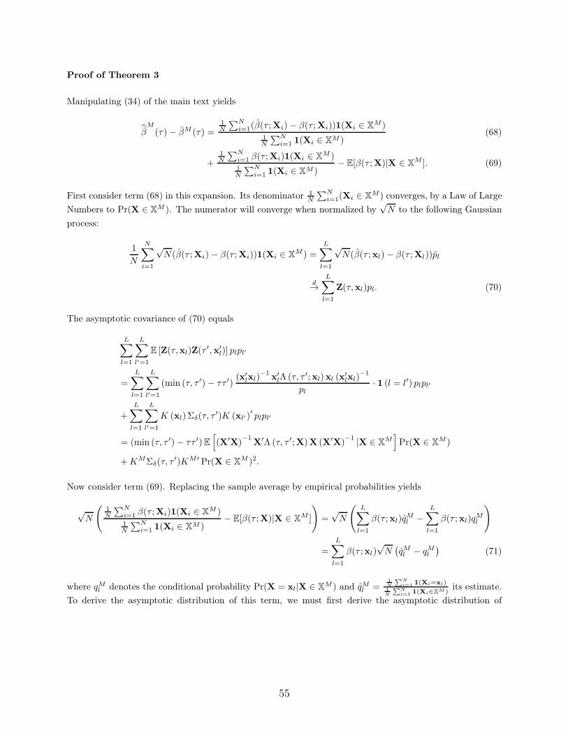
Proof of Theorem 3
Manipulating (34) of the main text yields
βM
(τ) − βM (τ) =1N
∑Ni=1(β(τ ;Xi)− β(τ ;Xi))1(Xi ∈ XM )
1N
∑Ni=1 1(Xi ∈ XM )
(68)
+1N
∑Ni=1 β(τ ;Xi)1(Xi ∈ X
M )1N
∑Ni=1 1(Xi ∈ XM )
− E[β(τ ;X)|X ∈ XM ]. (69)
First consider term (68) in this expansion. Its denominator 1N
∑Ni=1(Xi ∈ XM ) converges, by a Law of Large
Numbers to Pr(X ∈ XM ). The numerator will converge when normalized by√N to the following Gaussian
process:
1
N
N∑
i=1
√N(β(τ ;Xi)− β(τ ;Xi))1(Xi ∈ X
M ) =
L∑
l=1
√N(β(τ ;xl)− β(τ ;Xl))pl
d→L∑
l=1
Z(τ,xl)pl. (70)
The asymptotic covariance of (70) equals
L∑
l=1
L∑
l′=1
E [Z(τ,xl)Z(τ′,x′
l)] plpl′
=
L∑
l=1
L∑
l′=1
(min (τ, τ ′)− ττ ′)(x′
lxl)−1
x′lΛ (τ, τ ′;xl)xl (x
′lxl)
−1
pl· 1 (l = l′) plpl′
+
L∑
l=1
L∑
l′=1
K (xl)Σδ(τ, τ′)K (xl′ )
′plpl′
= (min (τ, τ ′)− ττ ′)E[(X′
X)−1
X′Λ (τ, τ ′;X)X (X′
X)−1 |X ∈ X
M]Pr(X ∈ X
M )
+KMΣδ(τ, τ′)KM′ Pr(X ∈ X
M )2.
Now consider term (69). Replacing the sample average by empirical probabilities yields
√N
(1N
∑Ni=1 β(τ ;Xi)1(Xi ∈ XM )1N
∑Ni=1 1(Xi ∈ XM )
− E[β(τ ;X)|X ∈ XM ]
)=
√N
(L∑
l=1
β(τ ;xl)qMl −
L∑
l=1
β(τ ;xl)qMl
)
=
L∑
l=1
β(τ ;xl)√N(qMl − qMl
)(71)
where qMl denotes the conditional probability Pr(X = xl|X ∈ XM ) and qMl =1N
∑Ni=1 1(Xi=xl)
1N
∑Ni=1 1(Xi∈XM )
its estimate.
To derive the asymptotic distribution of this term, we must first derive the asymptotic distribution of
55

qMl − qMl . Begin with the fact that
√N
1N
∑Ni=1 1(Xi = x1)− p1
...1N
∑Ni=1 1(Xi = xL)− pL
1N
∑Ni=1 1(Xi ∈ XM )− Pr(Xi ∈ XM )
d→ N
0...
0
0
,
p1(1− p1) · · · −p1pL p1(1− Pr(X ∈ XM ))...
. . ....
...
−p1pL · · · pL(1− pL) pL(1− Pr(X ∈ XM ))
p1(1− Pr(X ∈ XM )) · · · pL(1 − Pr(X ∈ X
M )) Pr(X ∈ XM )(1 − Pr(X ∈ X
M ))
(72)
and use the delta method to show
√N
qM1 − qM1...
qML − qML
d→ N(0L,ΣqM
)(73)
where
ΣqM =1
Pr(X ∈ XM )
qM1 (1− qM1 ) · · · −qM1 qML...
. . ....
−qM1 qML · · · qML (1− qML )
. (74)
Note that some of these limiting variance matrices are singular. Putting things together yields an asymptotic
variance-covariance for (71) of
L∑
l=1
L∑
l′=1
β(τ ;xl)ΣqM (l, l′)β(τ ′;xl′ )′ (75)
=1
Pr(Xi ∈ XM )
L∑
l=1
L∑
l′=1
β(τ ;xl)(qMl 1(l = l′)− qMl qMl′ )β(τ
′;xl′)′
=1
Pr(X ∈ XM )
(E[β(τ ;X)β(τ ′;X)′|X ∈ X
M]− E
[β(τ ;X)|X ∈ X
M]E[β(τ ′;X)|X ∈ X
M]′)
=C(β(τ ;X), β(τ ′;X)|X ∈ XM )
P(X ∈ XM ). (76)
Terms (70) and (71) are asymptotically independent, since the variation of (70) is conditional on X, while
the variation of (71) depends on X alone. Therefore, the limiting covariance of βM
(τ) is the sum of the
covariances of its two components, which yields the claimed result.
Proof of Theorem 4
There are two main steps to the proof. The first is to recover an estimate of the distribution function of
56
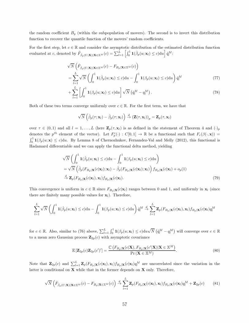
the random coefficient Bp (within the subpopulation of movers). The second is to invert this distribution
function to recover the quantile function of the movers’ random coefficients.
For the first step, let c ∈ R and consider the asymptotic distribution of the estimated distribution function
evaluated at c, denoted by Fβp(U ;X)|X∈XM (c) =∑L
l=1
[´ 1
01(βp(u;xl) ≤ c)du
]qMl :
√N(Fβp(U ;X)|X∈XM (c)− FBp|X∈XM (c)
)
=
L∑
l=1
√N
(ˆ 1
0
1(βp(u;xl) ≤ c)du −ˆ 1
0
1(βp(u;xl) ≤ c)du
)qMl (77)
+
L∑
l=1
[ˆ 1
0
1(βp(u;xl) ≤ c)du
]√N(qMl − qMl
). (78)
Both of these two terms converge uniformly over c ∈ R. For the first term, we have that
√N(βp(τ ;xl)− βp(τ ;xl)
)d→ (Z(τ,xl))p = Zp(τ,xl)
over τ ∈ (0, 1) and all l = 1, . . . , L (here Zp(τ,xl) is as defined in the statement of Theorem 4 and (·)pdenotes the pth element of the vector). Let F c
p (·) : C[0, 1] → R be a functional such that Fc(β(·,x)) =´ 1
0 1(βp(u;x) ≤ c)du. By Lemma 8 of Chernozhukov, Fernandez-Val and Melly (2012), this functional is
Hadamard differentiable and we can apply the functional delta method, yielding
√N
(ˆ 1
0
1(βp(u;xl) ≤ c)du−ˆ 1
0
1(βp(u;xl) ≤ c)du
)
=√N(βp(FBp|X(c|xl);xl)− βp(FBp|X(c|xl);xl)
)fBp|X(c|xl) + op(1)
d→ Zp(FBp|X(c|xl),xl)fBp|X(c|xl). (79)
This convergence is uniform in c ∈ R since FBp|X(c|xl) ranges between 0 and 1, and uniformly in xl (since
there are finitely many possible values for xl). Therefore,
L∑
l=1
√N
(ˆ 1
0
1(βp(u;xl) ≤ c)du−ˆ 1
0
1(βp(u;xl) ≤ c)du
)qMl
d→L∑
l=1
Zp(FBp|X(c|xl),xl)fBp|X(c|xl)qMl
for c ∈ R. Also, similar to (76) above,∑L
l=1
´ 1
0 1(βp(u;xl) ≤ c)du√N(qMl − qMl
)will converge over c ∈ R
to a mean zero Gaussian process Z2p(c) with asymptotic covariance
E [Z2p(c)Z2p(c′)′] =
C(FBp|X(c|X), FBp|X(c′|X)|X ∈ XM
)
Pr (X ∈ XM ). (80)
Note that Z2p(c) and∑L
l=1 Zp(FBp|X(c|xl),xl)fBp|X(c|xl)qMl are uncorrelated since the variation in the
latter is conditional on X while that in the former depends on X only. Therefore,
√N(Fβp(U ;X)|X∈XM (c)− FBp|X∈XM (c)
)d→
L∑
l=1
Zp(FBp|X(c|xl),xl)fBp|X(c|xl)qMl + Z2p(c) (81)
57

over c ∈ R.
We now turn to step two of the proof: inverting the distribution of the random coefficient to recover the
distribution of its quantiles. By assumption 5, Bp is assumed to have bounded support and fBp|X∈XM (c)
is strictly positive for all c ∈ R. Therefore by Kosorok (2007, Lemma 12.8 part (ii)) the inverse func-
tional is Hadamard differentiable into D(0, 1), the space of left-continuous functions with right-hand limits.
Evaluating this inverse at c = βMp (τ) yields
√N(βMp (τ) − βM
p (τ))
d→∑L
l=1 Zp(FBp|X(βMp (τ)|xl),xl)fBp|X(βM
p (τ)|xl)qMl + Z2p(β
Mp (τ))
fBp|X∈XM (βMp (τ))
= Zβp(τ) (82)
uniformly over τ ∈ (0, 1). To conclude the proof, we evaluate E[Zβp
(τ)Zβp(τ ′)′
], the asymptotic covariance
of this Gaussian process:
E
[Zβp
(τ)Zβp(τ ′)
′]
=
∑Ll=1
∑Ll′=1 fBp|X(βM
p (τ)|xl)e′pΣ(τ, FBp|X(βM
p (τ)|xl),xl), τ′, FBp|X(βM
p (τ ′)|xl′ ),xl′))epfBp|X(βMp (τ ′)|xl′ )q
Ml qMl′
fBp|X∈XM (βMp (τ))fBp|X∈XM (βM
p (τ ′))
+E[Z2p(β
Mp (τ))Z2p(β
Mp (τ ′))
]
fBp|X∈XM (βMp (τ))fBp|X∈XM (βM
p (τ ′))
where
∑Ll=1
∑Ll′=1 fBp|X(βM
p (τ)|xl)qMl e′pΣ(τ, FBp|X(βM
p (τ)|xl),xl), τ′, FBp|X(βM
p (τ ′)|xl′ ),xl′ )epfBp|X(βMp (τ ′)|xl′ )q
Ml′
fBp|X∈XM (βMp (τ))fBp|X∈XM (βM
p (τ ′))
=1
Pr (X ∈ XM )E[(min
(FBp|X(βM
p (τ)|X), FBp |X(βMp (τ ′)|X)
)− FBp|X(βM
p (τ)|X)FBp |X(βMp (τ ′)|X)
)
× e′p (X′X)
−1X
′Λ(FBp|X(βM
p (τ)|X), FBp |X(βMp (τ ′)|X);X
)X (X′
X)−1
ep
fBp|X(βMp (τ)|X)fBp|X(βM
p (τ ′)|X)∣∣X ∈ X
M]
(83)
+ E
[fBp|X(βM
p (τ)|X)fBp|X(βMp (τ ′)|X)
e′pK (X) Σδ
(FBp|X(βM
p (τ)|X), FBp |X(βMp (τ ′)|X)
)K(X
)′ep
∣∣∣∣X ∈ XM , X ∈ X
M
](84)
= Υ3(τ, τ′) + Υ4(τ, τ
′),
where X is an independent copy of X. Also,
E[Z2p(β
Mp (τ))Z2p(β
Mp (τ ′))
]=
C(FBp|X(βM
p (τ)|X), FBp |X(βMp (τ ′)|X)|X ∈ XM
)
Pr (X ∈ XM )(85)
= Υ2(τ, τ′),
which agrees with the expressions in the statement of the Theorem.
58
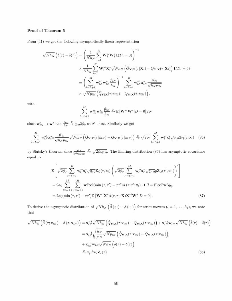
Proof of Theorem 5
From (41) we get the following asymptotically linear representation
√NhN
(δ(τ)− δ(τ)
)=
(1
NhN
N∑
i=1
W∗′i W
∗i 1(Di = 0)
)−1
× 1
NhN
N∑
i=1
W∗′i X
∗i
√NhN
(QY|X(τ |Xi)−QY|X(τ |Xi)
)1(Di = 0)
=
(M∑
l=L+1
w∗′lNw
∗lN
plNhN
)−1M∑
l=L+1
w∗′lNx
∗lN
plN√hNplN
×√NplN
(QY|X(τ |xlN )−QY|X(τ |xlN )
).
withM∑
l=L+1
w∗′lNw
∗lN
plNhN
p→ E [W∗′W
∗|D = 0] 2φ0
since w∗lN → w
∗l and plN
hN
p→ ql|02φ0 as N → ∞. Similarly we get
M∑
l=L+1
w∗′lNx
∗lN
plN√hNplN
√NplN
(QY|X(τ |xlN )−QY|X(τ |xlN )
)p→√2φ0
M∑
l=L+1
w∗′l x
∗l
√ql|0ZQ(τ,xl) (86)
by Slutsky’s theorem since plN√hNplN
p→ √2φ0ql|0. The limiting distribution (86) has asymptotic covariance
equal to
E
√2φ0
M∑
l=L+1
w∗′l x
∗l
√ql|0ZQ(τ,xl)
(√2φ0
M∑
l′=L+1
w∗′l′ x
∗l′√ql′|0pZQ(τ
′,xl′ )
)′
= 2φ0
M∑
l=L+1
M∑
l′=L+1
w∗′l x
∗l (min (τ, τ ′)− ττ ′)Λ (τ, τ ′;xl) · 1 (l = l′)x∗′
l w∗l ql|0
= 2φ0(min (τ, τ ′)− ττ ′)E[W
∗′X
∗Λ(τ, τ ′;X)X∗′W
∗|D = 0]. (87)
To derive the asymptotic distribution of√NhN
(β (·; ·)− β (·; ·)
)for strict movers (l = 1, . . . , L1), we note
that
√NhN
(β (τ ;xlN )− β (τ ;xlN )
)= x
−1lN
√NhN
(QY|X(τ |xlN )−QY|X(τ |xlN )
)+ x
−1lNwlN
√NhN
(δ(τ) − δ(τ)
)
= x−1lN
√hN
plN
√NplN
(QY|X(τ |xlN )−QY|X(τ |xlN )
)
+ x−1lNwlN
√NhN
(δ(τ) − δ(τ)
)
p→ x−1l wlZδ(τ) (88)
59

since hN
plN→ 0 for strict mover realizations. Finally, for near-stayers (l = L1 + 1, . . . , L) with DlN = hN :
√Nh3
N
(β (τ ;xlN )− β (τ ;xlN )
)= x
−1lN
√h3N
plN
√NplN
(QY|X(τ |xlN )−QY|X(τ |xlN )
)
+ x−1lNwlNhN
√NhN
(δ(τ) − δ(τ)
)
= x∗lN
hN
DlN
√hN
plN
√NplN
(QY|X(τ |xlN )−QY|X(τ |xlN )
)
+w∗lN
hN
DlN
√NhN
(δ(τ)− δ(τ)
)
D→ x∗l ZQ(τ,xl)√ql|02φ0
+w∗l Zδ(τ) (89)
since hN/DlN = 1 and by Slutsky’s Theorem. For near-stayers with DlN = −hN ,
√Nh3
N
(β (τ ;xlN )− β (τ ;xlN )
)D→ −x
∗l ZQ(τ,xl)√ql|02φ0
−w∗l Zδ(τ). (90)
Since ZQ(·,xl) and Zδ (·) are independent for l = 1, . . . , L, we can add the individual covariances of these
processes and get the desired result.
Proof of Theorem 6
We begin with the decomposition
√NhN
(βN (τ) − βN (τ))=√NhN
(βN (τ) − E[β(τ ;X)|X ∈ X
MN
])+√NhN
(E[β(τ ;X)|X ∈ X
MN
]− E [β(τ ;X)]
)
=
L∑
l=1
β(τ ;xlN )√NhN
(qMlN − qMlN
)(91)
+L∑
l=1
√NhN
(β(τ ;xlN )− β(τ ;xlN )
)qMlN (92)
+√NhN
(E[β(τ ;X)|X ∈ X
MN
]− E [β(τ ;X)]
). (93)
We first consider the joint asymptotic distribution of√NhN
(qMlN − qMlN
)for all l = 1, . . . , L. We start by
considering the asymptotic distribution of unconditional probabilities, which are normalized differently for
60
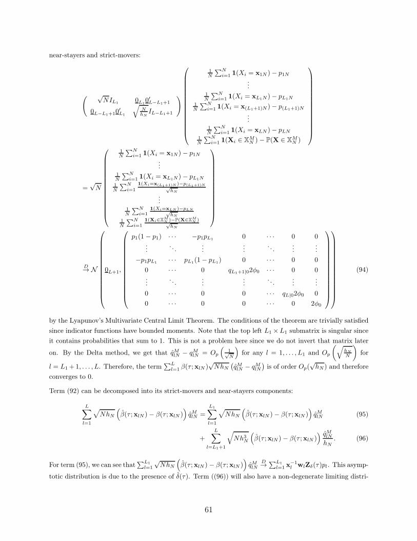
near-stayers and strict-movers:
( √NIL1 0L1
0′L−L1+1
0L−L1+10′L1
√NhN
IL−L1+1
)
1N
∑Ni=1 1(Xi = x1N )− p1N
...1N
∑Ni=1 1(Xi = xL1N )− pL1N
1N
∑Ni=1 1(Xi = x(L1+1)N )− p(L1+1)N
...1N
∑Ni=1 1(Xi = xLN )− pLN
1N
∑Ni=1 1(Xi ∈ XM
N )− P(X ∈ XMN )
=√N
1N
∑Ni=1 1(Xi = x1N )− p1N
...1N
∑Ni=1 1(Xi = xL1N )− pL1N
1N
∑Ni=1
1(Xi=x(L1+1)N )−p(L1+1)N√hN
...1N
∑Ni=1
1(Xi=xLN )−pLN√hN
1N
∑Ni=1
1(Xi∈XMN )−P(X∈X
MN )√
hN
D→ N
0L+1,
p1(1 − p1) · · · −p1pL1 0 · · · 0 0...
. . ....
.... . .
......
−p1pL1 · · · pL1(1− pL1) 0 · · · 0 0
0 · · · 0 qL1+1|02φ0 · · · 0 0...
. . ....
.... . .
......
0 · · · 0 0 · · · qL|02φ0 0
0 · · · 0 0 · · · 0 2φ0
(94)
by the Lyapunov’s Multivariate Central Limit Theorem. The conditions of the theorem are trivially satisfied
since indicator functions have bounded moments. Note that the top left L1 ×L1 submatrix is singular since
it contains probabilities that sum to 1. This is not a problem here since we do not invert that matrix later
on. By the Delta method, we get that qMlN − qMlN = Op
(1√N
)for any l = 1, . . . , L1 and Op
(√hN
N
)for
l = L1 +1, . . . , L. Therefore, the term∑L
l=1 β(τ ;xlN )√NhN
(qMlN − qMlN
)is of order Op(
√hN ) and therefore
converges to 0.
Term (92) can be decomposed into its strict-movers and near-stayers components:
L∑
l=1
√NhN
(β(τ ;xlN )− β(τ ;xlN )
)qMlN =
L1∑
l=1
√NhN
(β(τ ;xlN )− β(τ ;xlN )
)qMlN (95)
+
L∑
l=L1+1
√Nh3
N
(β(τ ;xlN )− β(τ ;xlN )
) qMlNhN
. (96)
For term (95), we can see that∑L1
l=1
√NhN
(β(τ ;xlN )− β(τ ;xlN )
)qMlN
D→∑L1
l=1 x−1l wlZδ(τ)pl. This asymp-
totic distribution is due to the presence of δ(τ). Term ((96)) will also have a non-degenerate limiting distri-
61

bution:
L∑
l=L1+1
√Nh3
N
(β(τ ;xlN )− β(τ ;xlN )
) qMlNhN
D→L∑
l=L1+1
Z(τ,xl)ql|02φ0 (97)
sinceqMlNh
p→ 2φ0ql|0. The asymptotic covariance of (92) will then be
= (min (τ, τ ′)− ττ ′)L∑
l=L1+1
L∑
l′=L1+1
x∗lΛ (τ, τ ′;xl)x
∗′l · 1 (l = l′) ql|02φ0
+
(L∑
l=L1+1
w∗l ql|02φ0 +
L1∑
l=1
x−1l wlpl
)Σδ(τ, τ
′)
(L∑
l′=L1+1
w∗l′ql′|02φ0 +
L1∑
l′=1
x−1l′ wl′pl′
).
We now show that Ξ0 = limN→∞
EN
[X
−1W||D| ≥ hN
]=∑L
l=L1+1 w∗l ql|02φ0 +
∑L1
l=1 x−1l wlpl:
limN→∞
EN
[X
−1W||D| ≥ hN
]= lim
N→∞
L∑
l=1
x−1lNwlNqMlN
= limN→∞
L∑
l=L1+1
w∗lN
Pr(X = xlN |D = |hN |)1− 2φ0hN
2φ0 + limN→∞
L1∑
l=1
x−1lNwlN
plN1− 2bhN
=
L∑
l=L1+1
w∗l ql|02φ0 +
L1∑
l=1
x−1l wlpl
by continuity in N .
Finally, we consider the bias term (93). We see that
√NhN
(EN
[β(τ ;X)|X ∈ X
MN
]− EN [β(τ ;X)]
)=√NhN
(L∑
l=1
β(τ ;xlN )qMlN −M∑
l=1
β(τ ;xlN )plN
)
=L∑
l=1
β(τ ;xlN )√NhN
(qMlN − plN
)−
M∑
l=L+1
β(τ ;xlN )√NhNplN .
We see that for l = 1, . . . , L,√Nh
(qMlN − plN
)= plN
2φ0
√Nh3
N
1−2φ0hN→ 0 since plN = O(1) and Nh3
N → 0. For
stayer realizations l = L + 1, . . . ,M , we have√NhNplN → 0 since
∑Ml=L+1 plN = 2φ0hN and Nh3
N → 0.
Therefore, term (93) converges to 0.
Proof of Theorem 7
We start by deriving the asymptotic distribution of the empirical cumulative distribution function of βp(U ;X)
with U distributed uniformly on [0, 1] independently of X, while conditioning on X ∈ XMN . The CDF estimand
62
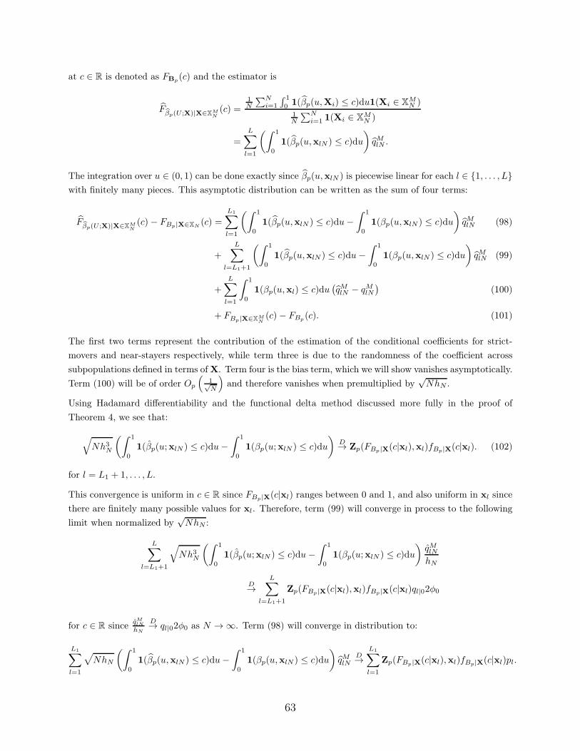
at c ∈ R is denoted as FBp(c) and the estimator is
Fβp(U ;X)|X∈XM
N
(c) =1N
∑Ni=1
´ 1
0 1(βp(u,Xi) ≤ c)du1(Xi ∈ XMN )
1N
∑Ni=1 1(Xi ∈ XM
N )
=L∑
l=1
(ˆ 1
0
1(βp(u,xlN ) ≤ c)du
)qMlN .
The integration over u ∈ (0, 1) can be done exactly since βp(u,xlN ) is piecewise linear for each l ∈ {1, . . . , L}with finitely many pieces. This asymptotic distribution can be written as the sum of four terms:
Fβp(U ;X)|X∈XM
N
(c)− FBp|X∈XN(c) =
L1∑
l=1
(ˆ 1
0
1(βp(u,xlN ) ≤ c)du−ˆ 1
0
1(βp(u,xlN ) ≤ c)du
)qMlN (98)
+
L∑
l=L1+1
(ˆ 1
0
1(βp(u,xlN ) ≤ c)du−ˆ 1
0
1(βp(u,xlN ) ≤ c)du
)qMlN (99)
+
L∑
l=1
ˆ 1
0
1(βp(u,xl) ≤ c)du(qMlN − qMlN
)(100)
+ FBp|X∈XMN(c)− FBp
(c). (101)
The first two terms represent the contribution of the estimation of the conditional coefficients for strict-
movers and near-stayers respectively, while term three is due to the randomness of the coefficient across
subpopulations defined in terms of X. Term four is the bias term, which we will show vanishes asymptotically.
Term (100) will be of order Op
(1√N
)and therefore vanishes when premultiplied by
√NhN .
Using Hadamard differentiability and the functional delta method discussed more fully in the proof of
Theorem 4, we see that:
√Nh3
N
(ˆ 1
0
1(βp(u;xlN ) ≤ c)du−ˆ 1
0
1(βp(u;xlN ) ≤ c)du
)D→ Zp(FBp|X(c|xl),xl)fBp|X(c|xl). (102)
for l = L1 + 1, . . . , L.
This convergence is uniform in c ∈ R since FBp|X(c|xl) ranges between 0 and 1, and also uniform in xl since
there are finitely many possible values for xl. Therefore, term (99) will converge in process to the following
limit when normalized by√NhN :
L∑
l=L1+1
√Nh3
N
(ˆ 1
0
1(βp(u;xlN ) ≤ c)du−ˆ 1
0
1(βp(u;xlN ) ≤ c)du
)qMlNhN
D→L∑
l=L1+1
Zp(FBp|X(c|xl),xl)fBp|X(c|xl)ql|02φ0
for c ∈ R sinceqMlNhN
D→ ql|02φ0 as N → ∞. Term (98) will converge in distribution to:
L1∑
l=1
√NhN
(ˆ 1
0
1(βp(u,xlN ) ≤ c)du−ˆ 1
0
1(βp(u,xlN ) ≤ c)du
)qMlN
D→L1∑
l=1
Zp(FBp|X(c|xl),xl)fBp|X(c|xl)pl.
63
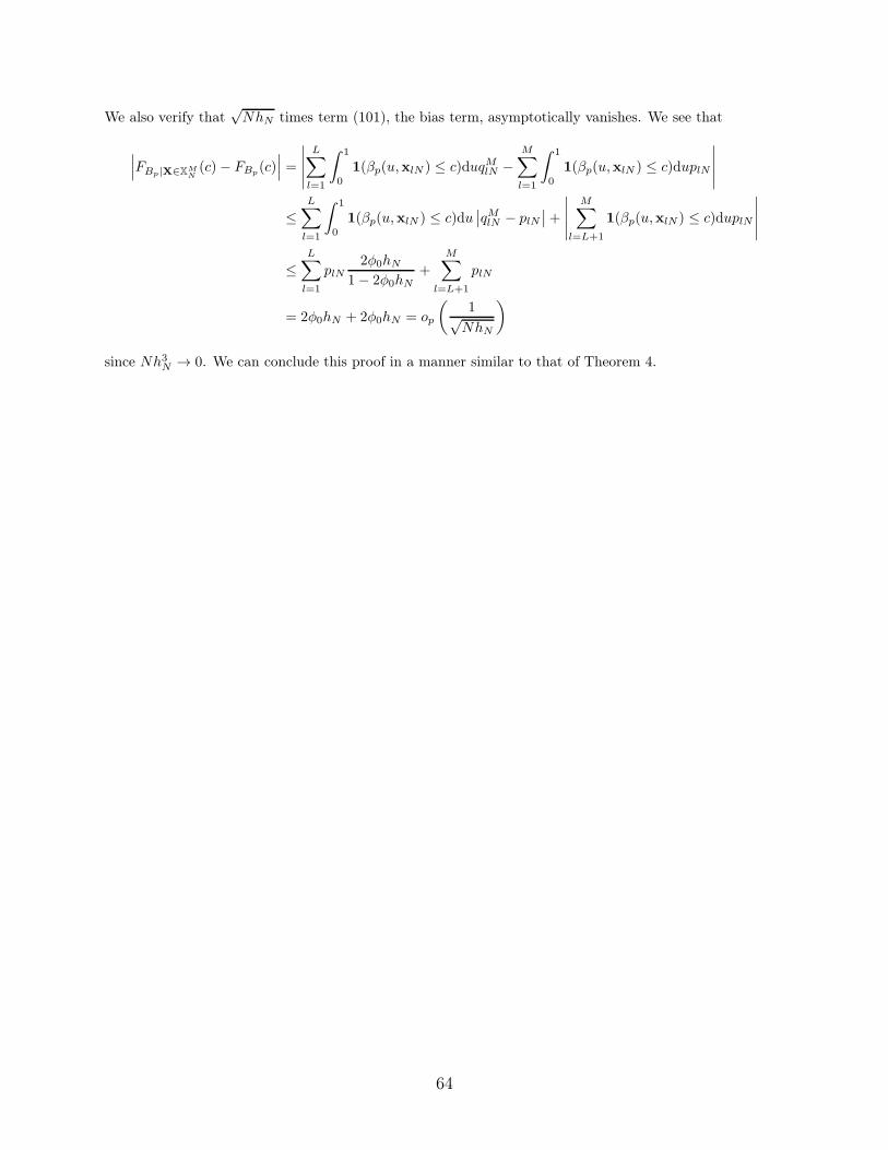
We also verify that√NhN times term (101), the bias term, asymptotically vanishes. We see that
∣∣∣FBp|X∈XMN(c)− FBp
(c)∣∣∣ =
∣∣∣∣∣
L∑
l=1
ˆ 1
0
1(βp(u,xlN ) ≤ c)duqMlN −M∑
l=1
ˆ 1
0
1(βp(u,xlN ) ≤ c)duplN
∣∣∣∣∣
≤L∑
l=1
ˆ 1
0
1(βp(u,xlN ) ≤ c)du∣∣qMlN − plN
∣∣+∣∣∣∣∣
M∑
l=L+1
1(βp(u,xlN ) ≤ c)duplN
∣∣∣∣∣
≤L∑
l=1
plN2φ0hN
1− 2φ0hN
+
M∑
l=L+1
plN
= 2φ0hN + 2φ0hN = op
(1√NhN
)
since Nh3N → 0. We can conclude this proof in a manner similar to that of Theorem 4.
64