1 3

DOI 10.1007/s00382-015-2860-2Clim Dyn (2016) 47:637–649

ORIGINAL ARTICLE

Quantifying the uncertainty of the annular mode time scale and the role of the stratosphere

Junsu Kim1,2 · Thomas Reichler1

Received: 13 January 2015 / Accepted: 25 September 2015 / Published online: 5 October 2015 © Springer-Verlag Berlin Heidelberg 2015

mode time scale over the Northern Hemisphere is similarly variable, there is no guarantee that the historical reanalysis record is a fully representative target for model evaluation. Over the Southern Hemisphere, however, the discrepancies between model and reanalysis are sufficiently large to con-clude that the model is unable to reproduce the observed time scale structure correctly. The effects of ocean coupling lead to a considerable increase in time scale and uncer-tainty in time scale, effects which are noticeable in both troposphere and stratosphere. We further use the model simulation to investigate the dynamical coupling between the stratosphere and the troposphere from the perspective of the annular mode time scale. Over the Northern Hemi-sphere, we find only weak indication for influences from stratosphere–troposphere coupling on the annular mode time scale. The situation is very different over the South-ern Hemisphere, where we find robust connections between the annular mode time scale in the stratosphere and that in the troposphere, confirming and extending earlier results of influences of stratospheric variability on the troposphere.

Keywords Annular mode time scale · Internal variability · Stratosphere–troposphere coupling · Dynamical sensitivity

1 Introduction

Climate sensitivity is a remarkably important characteristic of climate because many aspects of climate change scale almost linearly with it (Meehl et al. 2007). Research on climate sensitivity has now been ongoing for decades, but despite this the estimated range of climate sensitivity and the associated uncertainty essentially remained unchanged over this period (Knutti et al. 2006; Houghton et al. 2001;

Abstract The proper simulation of the annular mode time scale may be regarded as an important benchmark for cli-mate models. Previous research demonstrated that this time scale is systematically overestimated by climate models. As suggested by the fluctuation–dissipation theorem, this may imply that climate models are overly sensitive to external forcings. Previous research also made it clear that calcu-lating the AM time scale is a slowly converging process, necessitating relatively long time series and casting doubts on the usefulness of the historical reanalysis record to con-strain climate models in terms of the annular mode time scale. Here, we use long control simulations with the cou-pled and uncoupled version of the GFDL climate model, CM2.1 and AM2.1, respectively, to study the effects of internal atmospheric variability and forcing from the lower boundary on the stability of the annular mode time scale. In particular, we ask whether a model’s annular mode time scale and dynamical sensitivity can be constrained from the 50-year-long reanalysis record. We find that internal variability attaches large uncertainty to the annular mode time scale when diagnosed from decadal records. Even under the fixed forcing conditions of our long control run at least 100 years of data are required in order to keep the uncertainty in the annular mode time scale of the Northern Hemisphere to 10 %; over the Southern Hemisphere, the required length increases to 200 years. If nature’s annular

* Junsu Kim junsu.kim@snu.ac.kr

1 Department of Atmospheric Sciences, University of Utah, 135 S 1460 East RM 819 (WBB), Salt Lake City, UT 84112-0110, USA

2 Present Address: School of Earth and Environmental Sciences, Seoul National University, Seoul, South Korea

638 J. Kim, T. Reichler

1 3

Randall et al. 2007). The main reasons for this lack of pro-gress are the shortage of reliable observations and uncer-tainties in the formulation of climate models.

Recently, it has been suggested that the persistence time scale of major modes of extratropical variability in the atmosphere, also known as the annular modes (Thomp-son and Wallace 2001), could provide another impor-tant measure of sensitivity (Gerber et al. 2008a; Ring and Plumb 2008; Chen and Plumb 2009). This measure has been termed “dynamical sensitivity” to emphasize that it expresses the sensitivity of the circulation to climate change (Grise and Polvani 2014). As predicted by the fluc-tuation–dissipation theorem (Leith 1975), the equilibrium response to external forcings and thus dynamical sensitiv-ity should be proportional to the persistence time scale of the annular modes (hereafter simply AM time scale or τ). Thus, comparing the time scale between models and obser-vations could provide a useful alternative for understanding how realistic a model’s dynamical sensitivity is.

Previous studies already investigated the AM time scale from observational (Baldwin et al. 2003) and modeling (Gerber et al. 2008a, b, 2010; Son et al. 2008) data. Gerber et al. (2008b, 2010) found that the AM time scale is sys-tematically overestimated in climate models, particularly during summer over the Southern Hemisphere (SH). Like-wise, the AM time scale seems to be unrealistically long in more simple models (Gerber et al. 2008a).

In order to test dynamical sensitivity using the AM time scale one needs to determine the time scale robustly. However, the AM time scale is highly sensitive to internal atmospheric variability, complicating reliable estimates. For example, Chan and Plumb (2009) find that in ideal-ized models irregular and unpredictable regime shifts of the jet stream interfere with the determination of the AM time scale. Further, Gerber et al. (2008a) suggest that about 30 years of perpetual January model simulations are required to determine a time scale of 25 days at a 10 % accuracy. However, their measure is only an approximation and does not take into account complicating effects from the annual cycle and from variations in external forcings in more realistic data.

The difficulty in determining τ becomes evident from Fig. 1, showing the reanalysis derived time scale as a func-tion of season and height for two 25-year-long non-over-lapping periods. Although the two resulting τ structures are similar, there exist also important differences that cast doubts on the interpretation of the outcomes. For exam-ple, the result from the first period suggests that the win-tertime peak in τ occurs first in the stratosphere and then in the troposphere, but the second period shows the oppo-site behavior. A similar analysis conducted by Baldwin et al. (2003) using the same data but for one longer period (1958–2002) suggests that the stratospheric peak in τ

precedes that in the troposphere, similar to what is shown in Fig. 1a for the first period. Some of these discrepan-cies might be related to inconsistencies in the reanalysis or trends associated with climate change. An equally valid explanation, however, is that the time scale is highly sensi-tive to natural variability in the underlying data and that the process of calculating the time scale converges only slowly to its actual value. In other words, 25 or 50 years of obser-vations may not be sufficient to derive a reliable estimate of τ.

The goal of the present study is to investigate the AM time scale in a model and to understand the role of inter-nal atmospheric variability for determining the time scale. We try to answer the practical question of how many years of data are actually required to reduce the uncertainty in τ below a certain level. A related question is to what extent differences between models and reanalysis are indica-tive for real model biases and to what extent they are sim-ply due to internal atmospheric variability, also known as noise. We address our questions from long control simula-tions with coupled and uncoupled climate models, which because of their long length allows us to answer these ques-tions with a high degree of certainty.

Examining the differences between the coupled and uncoupled model enables us to distinguish between the influences from internal atmospheric dynamics and that from persistent lower boundary condition forcing on the annular mode time scale and its uncertainty. To the extent that our models are representative for other models, our finding then provides new insight into the shortcoming of models in reproducing the observed time scale. As we will show, the limited length of the historical observations

Fig. 1 NAM time scale (in days) as a function of month of the year and pressure, derived from the first (1959–1983) and last 25 years (1984–2008) of the NCEP/NCAR reanalysis

639Quantifying the uncertainty of the annular mode time scale and the role of the stratosphere

1 3

combined with internal atmospheric variability leads to large uncertainty in determining the AM time scale. Over the Northern Hemisphere (NH), the reanalysis derived time scale therefore does not provide a useful constraint for dynamical sensitivity. The situation over the SH is some-what different in that we find that the model has a signifi-cant bias in reproducing the observed time scale structure.

Another question to be addressed in our study is whether the stratosphere has as a detectable influence on the trop-osphere in terms of τ. Such an influence might be related to a dynamical downward influence from the stratosphere into the troposphere. Based on the observation that the win-ter time peak in the tropospheric AM time scale over the Northern Hemisphere is preceded by a similar peak in the stratosphere, Baldwin et al. (2003) were the first to suggest that such an influence exists. More recently, Simpson et al. (2011) found that indeed a dynamically active stratosphere serves to lengthen the time scale of the tropospheric annu-lar mode during winter. In the present study we come to a similar conclusion, but we find that the strength of the cou-pling in terms of the time scale is weaker over the NH than over the SH.

The outline of this paper is as follows. In Sect. 2, we describe our data and methodology. Section 3 compares the observed AM time scale with that derived from the model simulation. In Sect. 4, we investigate the uncertainty of the AM time scale when the calculations are based on the 50-year-long historical record. Section 5 explores the extent to which agreement between model and observations based on 50 years of data can be used to evaluate a model. In Sect. 6 we investigate the connection between the strato-sphere and troposphere in terms of the time scale and find that there are important differences between the NH and the SH. In Sect. 7, we investigate the uncertainty of the AM time scale structure as a function of length of the under-lying data, which we hope provides useful information for other similar studies. Our final section offers a summary and interpretation of our results.

2 Data and methodology

2.1 Data

We use daily zonal mean geopotential height fields pole-ward of 20° from the National Centers for Environmen-tal Prediction/National Center for Atmospheric Research (NCEP/NCAR) reanalyses (Kalnay et al. 1996), which are widely employed in annular mode studies (Baldwin and Thompson 2009; Thompson and Wallace 2000). The rea-nalysis dataset is available at 17 vertical levels from 1000 to 10 hPa, and our calculations are based on the 50-year-long period from 1959 to 2008.

The model simulated annular mode data are derived from long control simulations performed with two models. First, we utilize a 4000-year-long preindustrial control run with the coupled climate model CM2.1, developed at the Geophysical Fluid Dynamics Laboratory (GFDL Global Atmospheric Model Development Team 2004; Delworth et al. 2006). Second, we utilize a 2000-year long control integration with the uncoupled atmosphere-only com-panion model of CM2.1, also known as AM2.1. The pre-scribed SST and sea ice distribution (hereafter simply SST) for the uncoupled model were derived from averaging the coupled model’s SST over many years (Staten et al. 2014). All external forcings (greenhouse gases, ozone, solar influ-ences, and aerosol) in both simulations were held fixed at preindustrial levels. The spatial resolution of both models in the atmosphere is 2 degree latitude by 2.5 degree lon-gitude with 24 vertical levels up to 10 hPa. The models produce realistic climates (Reichler and Kim 2008), and despite their relatively low vertical resolution, they simu-late the annular mode variability and its coupling between the stratosphere and troposphere quite well (Reichler et al. 2012).

2.2 Methodology

Our procedure to compute the annular mode indices follows the method proposed by Baldwin and Thompson (2009). Specifically, it is based on the leading empirical orthogo-nal function (EOF) of daily zonal mean geopotential height anomaly fields at each pressure level, with anomalies being defined as deviations from the daily varying climatology with the global mean removed. The annular mode index is the principal component time series of the leading EOF. Similar to previous studies (Gerber et al. 2008b; Baldwin et al. 2003), the AM time scale is defined as the e-folding time of the autocorrelation function of the annular mode index. The calculation of the autocorrelation function is based on the daily annular mode index time series for all years. To calculate the autocorrelation for a given day of the year, we multiply each year of the original annular mode time series with a Gaussian kernel with a full width at half maximum of 60 days centered on the day under con-sideration. The result is a time series with yearly oscillat-ing amplitudes, maximum amplitudes for dates close to the central date, and decreasing amplitudes for dates distant to it. We next create 180 similar time series, but at lags for ±1 to ±90 days with respect to the central date, and then corre-late each with the time series for the central date. Since the resulting autocorrelation function is far from exponential (Ambaum and Hoskins 2002) and since the e-folding time scale is only meaningful if the autocorrelation function drops off exponentially, we base the calculation of the time scale off an exponential least-square fit to the empirically

640 J. Kim, T. Reichler

1 3

determined autocorrelation function. The AM time scale is then given by the day the fitted autocorrelation function drops to a value of 1/e. We repeat these calculations for each day of the year.

The time scale from the models is calculated by split-ting the 4000 and 2000-year-long simulations into several N-year-long segments (denoted as model segments). In most cases, we use N = 50, which allows a nice compari-son with the reanalysis derived time scale and which results in 80 and 40, respectively, different segments. We calculate the AM time scale individually for each segment and then use the mean time scale from all segments as our best esti-mate. The variability of the AM time scale is derived from the standard deviation across all segments, and our measure of uncertainty is given by the ratio between the standard deviation and the mean.

3 Comparison between model and reanalysis

We begin with a comparison of reanalysis and model derived AM time scale. This discussion is based on Fig. 2, which shows the time scale structures of the Northern and Southern Annular Modes (NAM and SAM) derived from 50 years of reanalysis data and 4000 and 2000, respec-tively, years of model data. We first note that the AM time

scale calculated from zonal mean fields is very similar to that from using two-dimensional data (e.g., Figure 1 of Baldwin et al. 2003). Key features of the reanalysis-derived time scale structure are well captured by the models. This includes tropospheric peaks in the NAM during boreal winter and in the SAM during austral spring. Further, in the stratosphere both reanalysis and models exhibit much longer time scales than in the troposphere, with two distinct maxima at 10 hPa in summer and at 100 hPa in winter for the NAM, and a time scale that is long throughout the year for the SAM.

The model derived time scales also exhibit important differences with respect to the reanalyses. First, the trop-ospheric peaks both for NAM and SAM are too broad in the models, a deficiency common to many models (Ger-ber et al. 2008b, 2010). Second, the tropospheric peak of the NAM in the models occurs in February, which is about 1–2 months delayed with respect to the reanalyses. Third, the models generally underestimate the stratospheric AM time scales over both hemispheres, whereas they over-estimate the tropospheric time scale, particularly for the coupled model and in the SH. As predicted by the fluctua-tion–dissipation theorem, the linear relationship between AM time scale and dynamical sensitivity suggests that the model’s sensitivity is too large in the troposphere and prob-ably too small in the stratosphere to the extent that these

Fig. 2 NAM and SAM time scale (in days) for (top) NCEP/NCAR reanalysis (1959–2008), (middle) the coupled (CM, mean over eighty 50-year-long segments) and uncoupled (AM, mean over forty 50-year-long segments) models, and (bot-tom) the percentage differ-ence between the two models (CM-AM). The time scale at 1000 hPa is derived from zonal mean sea level pressure; for all other levels, zonal mean geo-potential heights are used

641Quantifying the uncertainty of the annular mode time scale and the role of the stratosphere

1 3

biases are related to internal atmospheric dynamics and not to external persistent forcings.

We now discuss in more detail the differences in time scale between the coupled and uncoupled simulations (Fig. 2g, h). The prevalence of reddish colors in the dif-ference plots indicates that, on average, the coupled model has a longer time scale than the uncoupled model. This effect is unsurprising as low-frequency variations of the ocean increase the atmosphere’s interannual variability and hence its time scale (Keeley et al. 2009). In addition, it is well known that prescribed SSTs induce artificially large turbulent heat fluxes at the atmosphere’s lower boundary, reduce atmospheric variability (Barsugli and Battisti 1998), and hence decrease atmospheric persistence. A third factor which may play some role is that the climatological base state between the two models is not exactly the same; this may cause subtle changes in the internal dynamics and pro-cesses that determine the time scale (e.g., positive dynami-cal feedbacks).

For the NAM (Fig. 2g), ocean coupling leads to a mod-est ~20 % increases in tropospheric τ (from ~9 to ~12 days) during winter and spring. Generally, this is the time when atmosphere–ocean interaction is strongest and the El Nino Southern Oscillation is most active. However, the exact rea-son why the coupling effect on τ is most pronounced dur-ing April is not clear to us. It may be related to the winter-to-summer transition of the atmospheric circulation, the timing of which is likely to be more variable in the cou-pled model. For the SAM (Fig. 2h), the increase in τ from ocean coupling is more robust (ca. +50 %) than for the NAM, it affects the entire atmospheric column, and is most

pronounced during SH summer (DJF). The peak influence during summer may be related to enhanced variability in the timing of the breakdown of the SH polar vortex, which is believed to be responsible for the overall increase in time scale during this time of the year.

4 Time scale uncertainty in the historical record

We next examine the uncertainties associated with the AM time scale when 50-year-long data such as the NCEP/NCAR reanalysis are available. To this end we split the 4000-year-long (2000-year-long) coupled (uncoupled) model simulation into eighty (forty) different 50-year-long segments and calculate the time scale individually for each segment. The standard deviation (or variability) amongst the eighty coupled model segments exhibits a similar struc-ture as the time scale itself. The variability of the NAM time scale of the coupled model (Fig. 3a) displays dis-tinct maxima of 4–5 days at 100 hPa in early winter and at 10 hPa in summer. In the lower stratosphere and in the troposphere, this large variability persists out to spring. A similar variability in the seasonal timing of the peak time scale of the NAM amongst individual 50 year selections of the same simulation was found by Simpson et al. (2011). The variability of the SAM time scale (Fig. 3b) is gener-ally much larger than that of the NAM, somewhat consist-ent with the larger magnitude of the SAM time scale itself (Fig. 2d). In the lower stratosphere and also in the tropo-sphere, the SAM time scale is most variable during late spring and early summer, exceeding values of 15 days.

Fig. 3 Variability and uncer-tainty of model derived time scale. Shown are (top) standard deviation of the time scale (in days), derived from 80 samples of 50-year-long segments from the coupled model (CM), (middle) uncertainty of the time scale of the coupled model (in %), given by the standard deviation divided by the mean uncertainty, and (bottom) the difference in uncertainty (in %) between the coupled and uncou-pled model. Using F-statistics and neglecting differences in mean timescale between the two models, differences in uncertainty of about 20 % are statistically significant

642 J. Kim, T. Reichler

1 3

The large variability of the NAM time scale in the lower stratosphere during winter is likely related to different forms of dynamical variability in the stratosphere, which includes strong vortex events as well as stratospheric sud-den warming (SSW)-like events. SSWs occur in winter and represent abrupt weakenings or even complete break-downs of the polar vortex, creating pronounced NAM variability in the lower stratosphere and also in the troposphere (Simp-son et al. 2011; Baldwin et al. 2003). The variable timing and long persistence of weak and strong vortex events and also their infrequent occurrence likely contribute to the wintertime maximum of the NAM time scale in the strato-sphere and troposphere (Fig. 2c). This and also interdecadal intermittency in the occurrence of SSWs (Schimanke et al. 2011; Reichler et al. 2012) help to explain the large winter-time variability of the NAM time scale (Fig. 3a). Over the SH there are no SSWs. Instead, during spring there is large variability in the exact timing of the annual breakdown of the polar vortex, which is an important factor for interan-nual variability in the SAM during this time of the year. This explains the increase in the SAM time scale (Fig. 2d) and its variability (Fig. 3b) during spring.

A more objective measure for the uncertainty of the AM time scale is derived by taking the ratio between the stand-ard deviation and the mean of the time scale (Fig. 3c, d). This eliminates the effect of the mean on the variability. In most cases the annular mode uncertainty derived from 50-year-long segments amounts to 10–20 % of the mean, but it occasionally exceeds 25 %. We note that the uncer-tainty structure of the NAM (Fig. 3c) closely resembles that of the standard deviation (Fig. 3a), whereas the SAM (Fig. 3b, d) does not show this effect.

The lower panels of Fig. 3 show the percentage differ-ence in uncertainty between the coupled and uncoupled model. The reddish colors indicate that ocean coupling

leads to a general increase in uncertainty, as one might expect from the added atmospheric variance from the lower boundary condition forcings. However, the struc-ture of uncertainty increase does not necessarily resemble the structure in time scale increase (Fig. 2g, h). In particu-lar for the NAM there are increases in uncertainty (up to 60 %) during most times of the year and throughout the entire atmosphere, which reflects intense vertical coupling between the surface, troposphere, and stratosphere. The situation for the SAM is somewhat different, with relatively modest increases in uncertainty concentrated in the strato-sphere and during SH spring. The weakness of the ocean coupling effect over the SH is perhaps related to the fact that the southern polar cap is entirely covered by land.

5 Comparison of model and reanalysis derived AM time scales

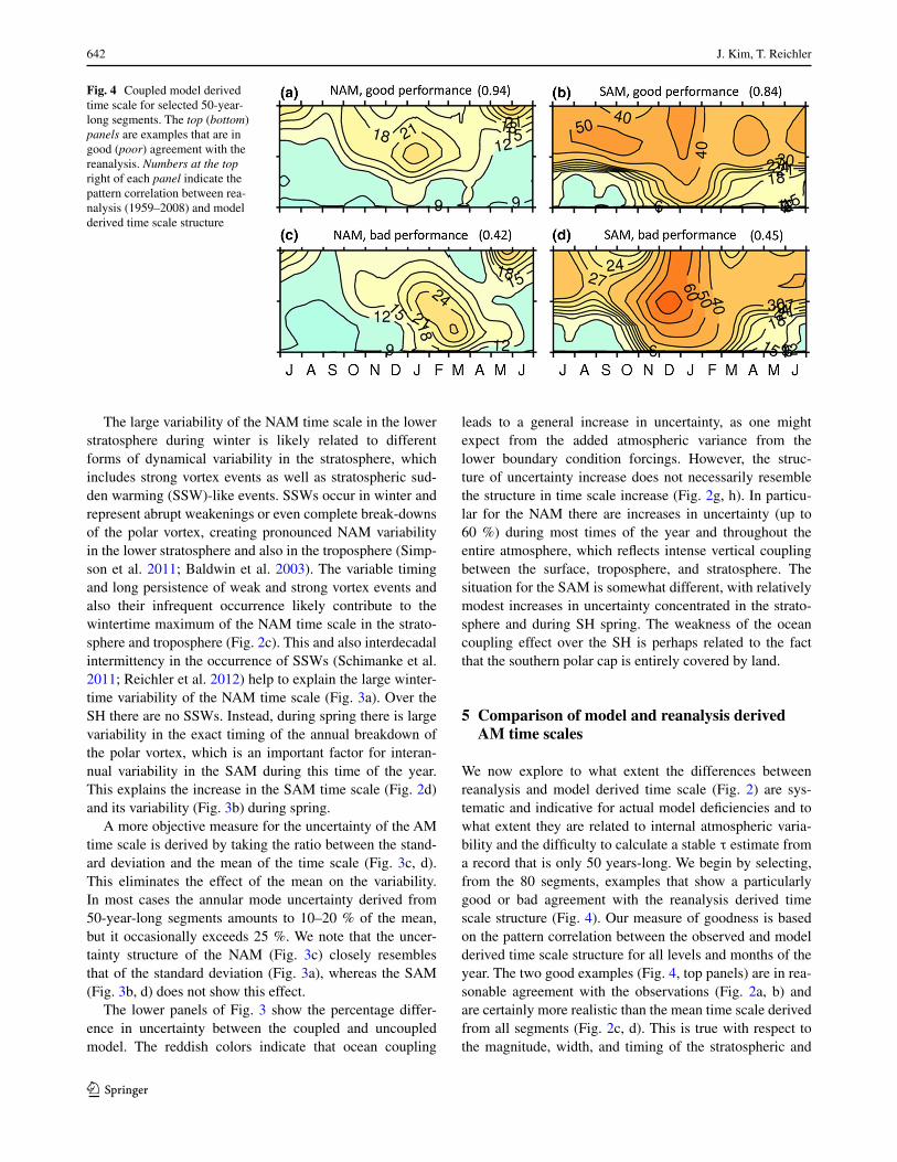
We now explore to what extent the differences between reanalysis and model derived time scale (Fig. 2) are sys-tematic and indicative for actual model deficiencies and to what extent they are related to internal atmospheric varia-bility and the difficulty to calculate a stable τ estimate from a record that is only 50 years-long. We begin by selecting, from the 80 segments, examples that show a particularly good or bad agreement with the reanalysis derived time scale structure (Fig. 4). Our measure of goodness is based on the pattern correlation between the observed and model derived time scale structure for all levels and months of the year. The two good examples (Fig. 4, top panels) are in rea-sonable agreement with the observations (Fig. 2a, b) and are certainly more realistic than the mean time scale derived from all segments (Fig. 2c, d). This is true with respect to the magnitude, width, and timing of the stratospheric and

Fig. 4 Coupled model derived time scale for selected 50-year-long segments. The top (bottom) panels are examples that are in good (poor) agreement with the reanalysis. Numbers at the top right of each panel indicate the pattern correlation between rea-nalysis (1959–2008) and model derived time scale structure

643Quantifying the uncertainty of the annular mode time scale and the role of the stratosphere

1 3

tropospheric peaks. The two examples of particularly poor agreement (bottom panels Fig. 4) hardly capture the observed seasonal cycle of the time scale, with peaks that have different timing, multiple maxima, no maxima, or are much too broad in structure. These examples demonstrate that internal variability has a huge effect on the outcomes of the time scale structure and that one must be cautious when judging models based on their performance in repro-ducing the observed time scale of the 50-year-long reanaly-sis record.

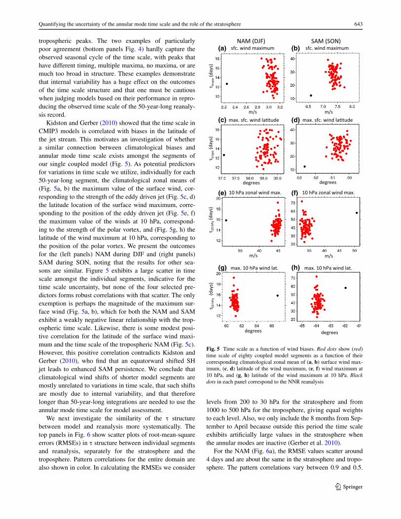
Kidston and Gerber (2010) showed that the time scale in CMIP3 models is correlated with biases in the latitude of the jet stream. This motivates an investigation of whether a similar connection between climatological biases and annular mode time scale exists amongst the segments of our single coupled model (Fig. 5). As potential predictors for variations in time scale we utilize, individually for each 50-year-long segment, the climatological zonal means of (Fig. 5a, b) the maximum value of the surface wind, cor-responding to the strength of the eddy driven jet (Fig. 5c, d) the latitude location of the surface wind maximum, corre-sponding to the position of the eddy driven jet (Fig. 5e, f) the maximum value of the winds at 10 hPa, correspond-ing to the strength of the polar vortex, and (Fig. 5g, h) the latitude of the wind maximum at 10 hPa, corresponding to the position of the polar vortex. We present the outcomes for the (left panels) NAM during DJF and (right panels) SAM during SON, noting that the results for other sea-sons are similar. Figure 5 exhibits a large scatter in time scale amongst the individual segments, indicative for the time scale uncertainty, but none of the four selected pre-dictors forms robust correlations with that scatter. The only exemption is perhaps the magnitude of the maximum sur-face wind (Fig. 5a, b), which for both the NAM and SAM exhibit a weakly negative linear relationship with the trop-ospheric time scale. Likewise, there is some modest posi-tive correlation for the latitude of the surface wind maxi-mum and the time scale of the tropospheric NAM (Fig. 5c). However, this positive correlation contradicts Kidston and Gerber (2010), who find that an equatorward shifted SH jet leads to enhanced SAM persistence. We conclude that climatological wind shifts of shorter model segments are mostly unrelated to variations in time scale, that such shifts are mostly due to internal variability, and that therefore longer than 50-year-long integrations are needed to use the annular mode time scale for model assessment.

We next investigate the similarity of the τ structure between model and reanalysis more systematically. The top panels in Fig. 6 show scatter plots of root-mean-square errors (RMSEs) in τ structure between individual segments and reanalysis, separately for the stratosphere and the troposphere. Pattern correlations for the entire domain are also shown in color. In calculating the RMSEs we consider

levels from 200 to 30 hPa for the stratosphere and from 1000 to 500 hPa for the troposphere, giving equal weights to each level. Also, we only include the 8 months from Sep-tember to April because outside this period the time scale exhibits artificially large values in the stratosphere when the annular modes are inactive (Gerber et al. 2010).

For the NAM (Fig. 6a), the RMSE values scatter around 4 days and are about the same in the stratosphere and tropo-sphere. The pattern correlations vary between 0.9 and 0.5.

NAM (DJF) SAM (SON)

max. sfc. wind la!tude

10 hPa zonal wind max.

max. 10 hPa wind lat.

m/s m/s

m/sm/s

degrees degrees

degreesdegrees

(c) (d)

(e) (f)

(g) (h)

τ tro

po(d

ays)

τ 10

hPa

(day

s)τ t

ropo

(day

s)τ 1

0 hP

a(d

ays)

sfc. wind maximum sfc. wind maximum

max. sfc. wind la!tude

10 hPa zonal wind max.

max. 10 hPa wind lat.

(a) (b)

Fig. 5 Time scale as a function of wind biases. Red dots show (red) time scale of eighty coupled model segments as a function of their corresponding climatological zonal mean of (a, b) surface wind max-imum, (c, d) latitude of the wind maximum, (e, f) wind maximum at 10 hPa, and (g, h) latitude of the wind maximum at 10 hPa. Black dots in each panel correspond to the NNR reanalysis

644 J. Kim, T. Reichler

1 3

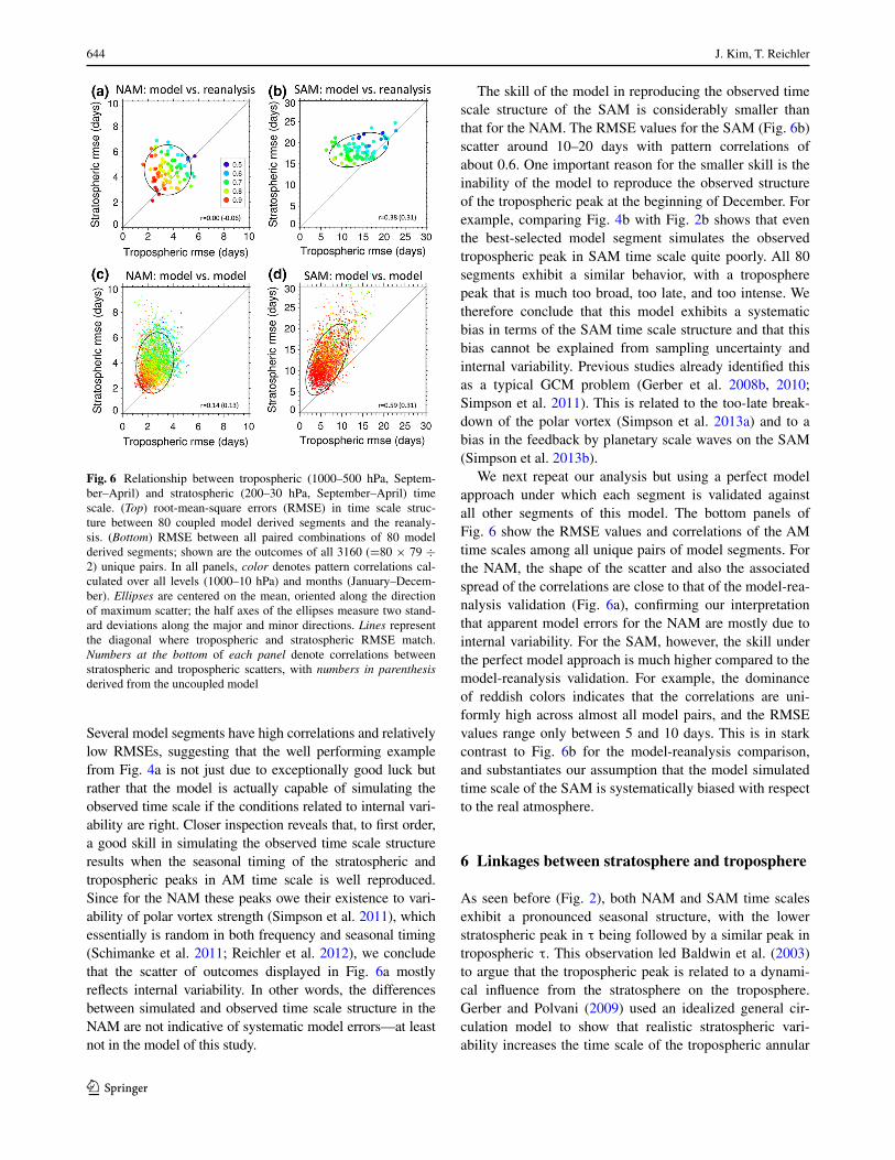
Several model segments have high correlations and relatively low RMSEs, suggesting that the well performing example from Fig. 4a is not just due to exceptionally good luck but rather that the model is actually capable of simulating the observed time scale if the conditions related to internal vari-ability are right. Closer inspection reveals that, to first order, a good skill in simulating the observed time scale structure results when the seasonal timing of the stratospheric and tropospheric peaks in AM time scale is well reproduced. Since for the NAM these peaks owe their existence to vari-ability of polar vortex strength (Simpson et al. 2011), which essentially is random in both frequency and seasonal timing (Schimanke et al. 2011; Reichler et al. 2012), we conclude that the scatter of outcomes displayed in Fig. 6a mostly reflects internal variability. In other words, the differences between simulated and observed time scale structure in the NAM are not indicative of systematic model errors—at least not in the model of this study.

The skill of the model in reproducing the observed time scale structure of the SAM is considerably smaller than that for the NAM. The RMSE values for the SAM (Fig. 6b) scatter around 10–20 days with pattern correlations of about 0.6. One important reason for the smaller skill is the inability of the model to reproduce the observed structure of the tropospheric peak at the beginning of December. For example, comparing Fig. 4b with Fig. 2b shows that even the best-selected model segment simulates the observed tropospheric peak in SAM time scale quite poorly. All 80 segments exhibit a similar behavior, with a troposphere peak that is much too broad, too late, and too intense. We therefore conclude that this model exhibits a systematic bias in terms of the SAM time scale structure and that this bias cannot be explained from sampling uncertainty and internal variability. Previous studies already identified this as a typical GCM problem (Gerber et al. 2008b, 2010; Simpson et al. 2011). This is related to the too-late break-down of the polar vortex (Simpson et al. 2013a) and to a bias in the feedback by planetary scale waves on the SAM (Simpson et al. 2013b).

We next repeat our analysis but using a perfect model approach under which each segment is validated against all other segments of this model. The bottom panels of Fig. 6 show the RMSE values and correlations of the AM time scales among all unique pairs of model segments. For the NAM, the shape of the scatter and also the associated spread of the correlations are close to that of the model-rea-nalysis validation (Fig. 6a), confirming our interpretation that apparent model errors for the NAM are mostly due to internal variability. For the SAM, however, the skill under the perfect model approach is much higher compared to the model-reanalysis validation. For example, the dominance of reddish colors indicates that the correlations are uni-formly high across almost all model pairs, and the RMSE values range only between 5 and 10 days. This is in stark contrast to Fig. 6b for the model-reanalysis comparison, and substantiates our assumption that the model simulated time scale of the SAM is systematically biased with respect to the real atmosphere.

6 Linkages between stratosphere and troposphere

As seen before (Fig. 2), both NAM and SAM time scales exhibit a pronounced seasonal structure, with the lower stratospheric peak in τ being followed by a similar peak in tropospheric τ. This observation led Baldwin et al. (2003) to argue that the tropospheric peak is related to a dynami-cal influence from the stratosphere on the troposphere. Gerber and Polvani (2009) used an idealized general cir-culation model to show that realistic stratospheric vari-ability increases the time scale of the tropospheric annular

Fig. 6 Relationship between tropospheric (1000–500 hPa, Septem-ber–April) and stratospheric (200–30 hPa, September–April) time scale. (Top) root-mean-square errors (RMSE) in time scale struc-ture between 80 coupled model derived segments and the reanaly-sis. (Bottom) RMSE between all paired combinations of 80 model derived segments; shown are the outcomes of all 3160 (=80 × 79 ÷ 2) unique pairs. In all panels, color denotes pattern correlations cal-culated over all levels (1000–10 hPa) and months (January–Decem-ber). Ellipses are centered on the mean, oriented along the direction of maximum scatter; the half axes of the ellipses measure two stand-ard deviations along the major and minor directions. Lines represent the diagonal where tropospheric and stratospheric RMSE match. Numbers at the bottom of each panel denote correlations between stratospheric and tropospheric scatters, with numbers in parenthesis derived from the uncoupled model

645Quantifying the uncertainty of the annular mode time scale and the role of the stratosphere

1 3

mode, confirming the earlier hypothesis from Baldwin et al. (2003). Similar conclusions were reached by Gerber et al. (2010), using a suite of stratosphere-resolving chem-istry climate models, and by Simpson et al. (2011), using the Canadian Middle Atmosphere Model. More precisely, Simpson et al. (2011) found that stratospheric variability approximately doubles the peak of the tropospheric SAM time scale, but that influences other than that from the strat-osphere also contribute to the long tropospheric SAM time scale. Here, we further address the issue of stratospheric influences on tropospheric time scale using our large ensembles with the coupled and uncoupled GFDL models, applying a different technique, and extending the analysis also to the NH.

We begin by investigating the relationship between strat-ospheric and tropospheric RMSE values from individual model segments of the coupled model when one validates against the reanalysis (top panels of Fig. 6). For the NAM (Fig. 6a), there is no obvious relationship between strato-spheric and tropospheric RMSE values as seen from the zero correlation of the scatter. For the SAM (Fig. 6b), how-ever, the two seem to be somewhat related, as shown by the modestly positive correlation (r = 0.38) of the scatter and the elliptical shape of its envelope. In other words, for an individual 50-year-long segment the time scale in the trop-osphere is generally better simulated when the time scale in the stratosphere is also well simulated, and vice versa. The connection between tropospheric and stratospheric time scale becomes even clearer when a perfect model approach is used to validate the model against itself (Fig. 6 bottom). As before, the correlations of the scatter are clearly posi-tive for the SAM (r = 0.59), and even for the NAM they are now somewhat positive (r = 0.14). This indicates that indeed stratospheric and tropospheric time scales are con-nected, and that in this model the connection is stronger for the SAM than for the NAM. The stronger SAM connection is consistent with the longer time scale of the tropospheric SAM as compared to that of the NAM, which according to the fluctuation–dissipation theorem should be associated with a stronger response to a given stratospheric forcing.

We further investigate the possible influence of the stratospheric time scale on the tropospheric time scale by focusing separately on the timing and on the strength of the peaks in τ (Fig. 7). To this end, we determine for all 50-year-long model segments the date and the strength of maximum τ in the lower troposphere (1000–500 hPa) and in the lower stratosphere (200–30 hPa). For the NAM, the stratospheric and tropospheric peaks occur between Novem-ber and March (Fig. 7a). The shape of the ellipses of maxi-mum scatter and also the correlation of the scatter itself show that the dates of the tropospheric peaks are essentially unrelated to the dates of the stratospheric peaks (r = 0.08). Also, most scatter symbols are located above the diagonal

line, indicating that the tropospheric peak dates usually lag the stratospheric peaks. Taking the mean over all segments (black circle in the center of the ellipses) we find that in the stratosphere the peak usually occurs during mid-January and in the troposphere at the beginning of March, which is a lag of several weeks. In contrast to the simulations, the rea-nalyses (black diamond) exhibit about a 1-week delay from the stratosphere into the troposphere and a peak date that occurs about 1 month earlier. Examining the magnitude of the peaks in τ for the NAM (Fig. 7c), we again find only a very weak connection between stratosphere and troposphere (r = 0.09). We note that, despite the differences in the mean timing, the outcomes for the segments as a whole are con-sistent with the reanalysis since the black diamond symbols for the reanalyses are located well within the uncertainty ellipses of the model. In other words, various segments have

Fig. 7 Relationship between stratospheric and tropospheric time scale maxima derived from 80 coupled model segments. a, b Date of lower stratospheric (200–30 hPa) and lower tropospheric (1000–500 hPa) time scale maxima (results are not sensitive to the exact choice of the vertical levels). c, d Relative strength of time scale maxima, given by the ratio of time scale maxima and the mean of all maxima (23 days for stratospheric NAM, 15 for tropospheric NAM, 71 for stratospheric SAM, and 47 for tropospheric SAM). Colored circles show outcomes from individual model segments and black circles indicate the mean. Ellipses are centered on the mean, oriented along the direction of maximum scatter, with the two axes showing four standard deviations along the major and minor direction. Numbers at the bottom are correlations between stratospheric and tropospheric scatters. Numbers in parenthesis indicate correlations derived from the uncoupled model. Black diamonds show outcomes from NCEP/NCAR reanalysis (1959–2008). Lines in top panels represent match-ing stratospheric and tropospheric date

646 J. Kim, T. Reichler

1 3

a NAM time scale structure that is similar to the reanalysis, both in terms of peak date and peak magnitude.

For the SAM there is somewhat less scatter in peak dates (Fig. 7b), but as for the NAM the peaks in the stratosphere mostly lead that in the troposphere, which may be some-what indicative for a stratospheric influence on the tropo-sphere. The SAM peak dates are centered on late Novem-ber in the stratosphere and on December in the troposphere. Comparing to the NAM and taking into account the sea-sonal shift of 6 months between the two hemispheres, the SAM dates are shifted late by about 4 months. This shift, which was also noted by Gerber et al. (2008b), is consistent with the fact that variability of the NAM is dominated by vacillations of the polar vortex during mid-winter whereas that of the SAM is related to the changing breakdown date of the polar vortex during spring. For the SAM the strato-spheric peak timing is somewhat correlated with the tropo-spheric peak (r = 0.20). The narrow range in timing and the moderately positive correlation between stratospheric and tropospheric peak timing is likely related to the smaller internal variability and non-existence of SSWs over the SH. As shown in Fig. 7d, there is much more scatter in the magnitude of the peak time scale for the SAM than for the NAM and a quite significant correlation between the strato-sphere and the troposphere (r = 0.72). The model outcomes are consistent with the reanalyses (black triangles) for the seasonal timing of the peak. This, however, is not true for the intensity of the peak time scale, which is significantly stronger in the model than for the reanalysis.

The above analysis (Figs. 6, 7) suggests that stratospheric and tropospheric time scale are somewhat connected, in par-ticular over the SH. However, this analysis is based on cou-pled model data, and it is still unclear to what extent the con-nection is due to oceanic variability influencing stratosphere and troposphere in similar ways and to what extent it is due to internal atmospheric processes. In order to shed somewhat more light on this question, we repeat our analysis using data from the uncoupled model, where oceanic variability can-not be the source or recipient of influence. The outcomes for the uncoupled model data (see numbers in parenthesis) are similar to the coupled model, except that the stratosphere-troposphere relationships become weaker for the SAM and stronger for the NAM. For example, the relatively tight corre-lation of r = 0.72 in SAM peak time scale reduces to r = 0.32 in the uncoupled model. Such a reduction is expected as ocean signals forcing the troposphere, stratosphere, or both are eliminated, and tropospheric variability is damped. In terms of peak time scale (Fig. 7c, d), the remaining relation-ship between stratosphere and troposphere is weakly positive (r ~ 0.3) and about the same for NAM and SAM. The small correlation is somewhat indicative for a stratospheric influ-ence in lengthening the tropospheric time scale.

7 Uncertainty in time scale

Calculating the time scale of the annular mode is a slowly converging procedure, and multi-decade-long data are needed to arrive at reasonable estimates. From Fig. 3 one can see that the uncertainty is ~15–25 % if the calculations are based on a 50-year-long record. This raises the more general question of how long of a record is required in order to limit the uncertainty of the time scale calculations to a certain value. Our long control simulations provide an excellent opportunity to answer this question by deriving empirical relationships between time scale uncertainty and length of the simulation period.

We employ a procedure similar to that of Fig. 3 and calculate a measure of uncertainty of the AM time scale by determining the standard deviation of the τ structure amongst multiple N-year-long model segments, averaged over all levels and all days of the year. We repeat the calcu-lation for increasing N = (10, 20, 50, 100, 200, 500 years), noting that the total number of segments decreases as N increases. In Fig. 8, the outcomes for the coupled and uncoupled model are shown by the red and blue symbols, respectively.

For a segment length of N = 10 years, the uncertainty is very large and amounts to 40–50 % of the mean time scale. As expected, the uncertainty and its range become smaller as N increases. In order to limit the uncertainty to 10 % at least N = 100 years of data are needed. The lines in Fig. 8 are extrapolations from the empirically determined values for N = 10 years, assuming that uncertainty for longer N scales inversely proportional to the square root of N. Such a scaling is intuitive if one assumes that calculating τ over increasing N is similar to taking the mean τ from multi-ple (=N/10) 10-year-long segments and knowing that the standard error of the mean equals the sample standard devi-ation divided by the square root of the sample size. One can see that the extrapolated values are very similar to the empirically determined ones. Therefore, it is reasonable to assume that the extrapolated uncertainties for the reanaly-sis (black curve) are good approximations for the actual (unknown) uncertainties.

Figure 8 also indicates that the uncertainty of the SAM is larger than that of the NAM (50 vs. 40 % for N = 10). Since our measure of uncertainty is relative to the mean, the increase is indicative for differences between NAM and SAM time scale that go beyond the simple effects of the mean.

Comparing the differences in NAM uncertainty from the coupled (red) and uncoupled (blue) model one finds that, as expected from Fig. 3e, the uncertainty of the uncoupled model is consistently lower, but the differences with respect to the coupled model are not very large. For the SAM, the

647Quantifying the uncertainty of the annular mode time scale and the role of the stratosphere

1 3

differences between coupled and uncoupled model time scale uncertainty are even smaller. In other words, averaged over the whole atmosphere and entire year, internal atmos-pheric dynamics dominate the uncertainty of the time scale, while effects from low-frequency lower boundary forcing are of second order.

We next test how our uncertainty estimate derived from dividing our long control runs into shorter segments com-pares with an alternate method suggested by Simpson et al. (2011). Simpson’s method is based on resampling one sin-gle relatively short time series using bootstrapping with

replacement to produce a large number of synthetic time scale estimates. We also apply Simpson’s approach, but instead of using just one arbitrary fifty-year-long model time series for the resampling, we utilize all 80 fifty-year long time series of our control run and average the results. In Fig. 9 we compare the outcomes from the two approaches for N = 50 years and a level of 500 hPa. It is reassuring to find that the two methods lead to very similar outcomes in terms of the mean time scale (top). However, resampling (dashed) consistently leads to somewhat larger uncertainty estimates than our approach (solid). Getting

Fig. 8 Uncertainty of NAM and SAM time scale structure (aver-ages over all levels and days of the year) as a function of length of the underlying time series for (black) the NCEP/NCAR reanalysis, (red) the coupled model, and (blue) the uncoupled model, all calcu-lated from multiple segments of given length N. Grey symbols indi-cate outcome for NCEP/NCAR reanalysis from using bootstrapping (100 times, with replacement) data within the N-year-long segments.

Uncertainty is defined as in Fig. 3. Circles are actual calculations (slightly shifted along the x-axis for clarity), and curves represent extrapolations from N = 10 years using the analytical expression (inversely proportional to the square root of the length of the seg-ment, see text). Error bars denote ±2 standard deviations from the mean, calculated from bootstrapping by randomly selecting a subset of five segments with replacement and repeating this 100 times

Fig. 9 Multiple samples versus bootstrapping in coupled model. Shown are (top) time scale at 500 hPa (in days) and (bottom) corre-sponding ± 2 standard deviation, derived from (solid) 80 fifty-year-

long samples and (dashed) bootstrapping (100 times) with replace-ment of N = 50 year-long samples

648 J. Kim, T. Reichler

1 3

back to Fig. 8, the grey symbols indicate uncertainty esti-mates for the NCEP/NCAR reanalysis using Simpson’s method, which can be compared with the black symbols. The small differences suggests that future studies can safely use Simpson’s method and that this perhaps leads to somewhat larger uncertainty estimates than our method. The huge benefit of Simpson’s approach is that long time series are not needed.

8 Summary and discussion

In this study we examined the AM time scale of the GFDL general circulation model CM2.1 and compared it against the NCEP/NCAR reanalysis. We investigated the overall time-height structure of the time scale and the seasonal timing and strength of the time scale maxima in the tropo-sphere and stratosphere. A particular focus was understand-ing the uncertainties associated with determining the time scale and also possible connections between stratospheric and tropospheric time scale. Overall, the model simulated time scale structure agreed reasonably well with that of the reanalysis, in particular in terms of the seasonal timing of the tropospheric peaks. However, a major model deficiency was the seasonal cycle of the time scale in the troposphere, which like in most models (Gerber et al. 2008b, 2010) was much too broad compared to the reanalysis.

An important theme of this study was the slow conver-gence of the time scale and the role of internal variability for the convergence. Gerber et al. (2008a) used theoretical arguments to estimate that if τ is 10 days about 10 years of a perpetual January integrations are necessary to deter-mine the time scale at 20 % accuracy. Multiplying this number by a factor of four to account for the seasonal cycle in our integrations one arrives at about 40 years of data, which agrees very well with our empirically derived results (Fig. 8). According to our long control run at least 100 years of integration are needed in order to limit the uncertainty below 10 %. At the same time, we find that the uncertainty of the SAM time scale is consistently larger than that of the NAM, which might be indicative for larger low-frequency variability in the SAM as compared to the NAM. Our uncertainty estimates agree well with an alter-nate method proposed by Simpson et al. (2011), which is based on resampling. Simpson’s method is preferable because it requires only short records, and, as we have shown, produces reasonable results.

The large time scale uncertainty also raises the ques-tion of whether the 50-year-long historical record is long enough to evaluate climate models. Since the uncertainty amounts to 20 % when only 50 years of data are available it is clear that caution is necessary when judging models in terms of their time scale agreement with the reanalysis.

Indeed, our analysis shows that for the NAM the reanalysis lies within the scatter of outcomes from individual 50-year-long model segments. This is not only true in terms of the overall time scale structure (Fig. 6) but also in terms of seasonal timing and magnitude of the winter maximum in NAM time scale (Fig. 7). Our results suggest that the differences between model and reanalysis can be largely explained from internal variability. Systematic model biases that would be indicative for unrealistic dynamical sensitivity could not be detected.

For the SAM, however, the above-described situation is different. For example, if the model is validated against itself under a perfect model approach, individual segments agree much better with each other than with the reanaly-sis. Further analysis shows that the disagreement between model and reanalysis for the SAM is mostly related to the magnitude of the spring/summer time maximum in tropo-spheric SAM time scale. On average and compared against the reanalysis, the model overestimates the strength of the peak in time scale by a factor of two. To the extent that this bias is associated with internal dynamics and not with overly persistent forcings, this indicates that the model’s tropospheric SAM is too sensitive with respect to external influences.

There has been some recent discussion about possible influences of stratospheric variability in lengthening the tropospheric AM time scale (Baldwin et al. 2003). Vari-ous previous modeling studies found conclusive evidence for such influences. We also investigated this question and found that in the coupled model the stratospheric connec-tion to the tropospheric time scale is weak at best over the NH and quite strong over the SH (Figs. 6, 7). The situa-tion in the uncoupled model is somewhat different, with a weaker connection over the SH and a stronger connec-tion over the NH. The correlation over the NH is still quite weak and therefore somewhat in disagreement with Simp-son et al. (2011), who state that “in the NH, virtually all of the seasonality in AM time scales arises from the down-ward influence of stratospheric annular mode variability”. It is likely that differences in how the two studies approach the question and how stratospheric variability is generated are responsible for the different conclusions.

The connection between stratospheric and tropospheric time scale in the model is quite pronounced over the SH in terms of the magnitude of the peak time scale (Fig. 7d). For the SAM, there is only a slight delay between stratospheric and tropospheric time scale maxima, and most model seg-ments suggest that over the SH the stratospheric peak leads the troposphere by a week or so. Further, there are no sig-nificant differences between model and reanalysis in terms of this lag over the SH. For the NH, the situation is very dif-ferent. Averaged over all model segments, the stratospheric peak in the NAM leads the tropospheric peak by about

649Quantifying the uncertainty of the annular mode time scale and the role of the stratosphere

1 3

2 months, which is unrealistically long when compared to the reanalysis (Figs. 2, 7). However, as noted above, many individual model segments are in perfect agreement with the reanalysis in terms of their timing of stratospheric and tropospheric peaks. Based on these results one must con-clude that differences in the stratosphere-troposphere lag between the mean model outcome and the reanalysis are not indicative for real model deficiencies, or that the lag of just a few days seen in the reanalysis is a characteristic fea-ture of our atmosphere.

Acknowledgments We thank the two anonymous reviewers for their constructive comments and suggestions, and the National Sci-ence Foundation for its financial support under Grant 1446292. We thank the University of Utah Center for High Performance Comput-ing (CHPC) and the National Energy Research Scientific Computing Center (NERSC) for computing support.

References

Ambaum MHP, Hoskins BJ (2002) The NAO troposphere-strato-sphere connection. J Clim 15:1969–1978

Baldwin MP, Thompson DWJ (2009) A critical comparison of stratosphere-troposphere coupling indices. Quart J R Met Soc 135:1661–1672

Baldwin MP, Stephenson DB, Thompson DWJ, Dunkerton TJ, Charl-ton AJ, Alan ON (2003) Stratospheric memory and skill of extended-range weather forecasts. Science 301:636–640

Barsugli JJ, Battisti DS (1998) The basic effects of atmosphere-ocean thermal coupling on midlatitude variability. J Atmos Sci 55:477–493

Chan CJ, Plumb RA (2009) The response to stratospheric forcing and its dependence on the state of the troposphere. J Atmos Sci 66:2107–2115

Chen G, Plumb RA (2009) Quantifying the eddy feedback and the persistence of the zonal index in an idealized atmospheric model. J Atmos Sci 66:3707–3720

Delworth TL et al (2006) GFDL’s CM2 global coupled climate mod-els. Part I: formulation and simulation characteristics. J Clim 19:643–674

Gerber EP, Polvani LM (2009) Stratosphere-troposphere coupling in a relatively simple AGCM: the importance of stratospheric vari-ability. J Clim 22:1920–1933

Gerber EP, Voronin S, Polvani LM (2008a) Testing the annular mode autocorrelation time scale in simple atmospheric general circula-tion models. Mon Wea Rev 136:1523–1536

Gerber EP, Polvani LM, Ancukiewicz D (2008b) Annular mode time scales in the Intergovernmental Panel on Climate Change Fourth Assessment Report models. Geophys Res Lett 35:L22707

Gerber EP et al (2010) Stratosphere-troposphere coupling and annu-lar mode variability in chemistry-climate models. J Geophys Res 115:D00M06

GFDL Global Atmospheric Model Development Team (2004) The new GFDL global atmosphere and land model AM2-LM2: eval-uation with prescribed SST simulations. J Clim 17:4641–4673

Grise KM, Polvani LM (2014) Is climate sensitivity related to dynam-ical sensitivity? A Southern Hemisphere perspective. Geophys Res Lett 41:534–540

Houghton JT et al (2001) Climate change 2001: The scientific basis. Cambridge University Press, Cambridge

Kalnay E et al (1996) The NCEP/NCAR 40-year reanalysis project. Bull Am Met Soc 77:437–471

Keeley SPE, Sutton RT, Shaffrey LC (2009) Does the North Atlan-tic oscillation show unusual persistence on intraseasonal time-scales? Geophys Res Lett 36:L22706

Kidston J, Gerber EP (2010) Intermodel variability of the poleward shift of the austral jet stream in the CMIP3 integrations linked to biases in 20th century climatology. Geophys Res Lett 37:L09708

Knutti R, Meehl GA, Allen MR, Stainforth DA (2006) Constraining climate sensitivity from the seasonal cycle in surface tempera-ture. J Clim 19:4224–4233

Leith CE (1975) Climate response and fluctuation dissipation. J Atmos Sci 32:2022–2026

Meehl GA et al (2007) Global Climate Projections. In: Solomon S, Qin D, Manning M, Chen Z, Marquis M, Averyt KB, Tignor M, Miller HL (eds) Climate Change 2007: The physical science basis. Contribution of Working Group I to the fourth assessment report of the intergovernmental panel on climate change. Cam-bridge University Press, Cambridge

Randall DA et al (2007) Cilmate models and their evaluation. In: Sol-omon S, Qin D, Manning M, Chen Z, Marquis M, Averyt KB, Tignor M, Miller HL (eds) Climate change 2007: The physical science basis. Contribution of working Group I to the fourth assessment report of the intergovernmental panel on climate change. Cambridge University Press, Cambridge

Reichler T, Kim J (2008) How well do coupled models simulate today’s climate? Bull Am Met Soc 89:303–311

Reichler T, Kim J, Manzini E, Kröger J (2012) A stratospheric con-nection to Atlantic climate variability. Nature Geos 5:783–787

Ring MJ, Plumb RA (2008) The response of a simplified GCM to axisymmetric forcings: applicability of the fluctuation–dissipa-tion theorem. J Atmos Sci 65:3880–3898

Schimanke S, Körper J, Spangehl T, Cubasch U (2011) Multi-decadal variability of sudden stratospheric warmings in an AOGCM. Geophys Res Lett 38:L01801

Simpson IR, Hitchcock P, Shepherd TG, Scinocca JF (2011) Strato-spheric variability and tropospheric annular-mode timescales. Geophys Res Lett 38:L20806

Simpson IR, Hitchcock P, Shepherd TG, Scinocca JF (2013a) South-ern annular mode dynamics in observations and models. Part I: the influence of climatological zonal wind biases in a compre-hensive GCM. J Clim 26:3953–3967

Simpson IR, Shepherd TG, Hitchcock P, Scinocca JF (2013b) South-ern annular mode dynamics in observations and models. Part II: Eddy Feedbacks. J Clim 26:5220–5241

Son S-W, Lee S, Feldstein SB, Ten Hoeve JE (2008) Time scale and feedback of zonal-mean-flow variability. J Atmos Sci 65:935–952

Staten PW, Reichler T, Lu J (2014) The transient circulation response to radiative forcings and sea surface warming. J Clim 27:9323–9336

Thompson DWJ, Wallace JM (2000) Annular modes in the extrat-ropical circulation. Part I: Month-to-month variability. J Clim 13:1000–1016

Thompson DWJ, Wallace JM (2001) Regional climate impacts of the Northern Hemisphere annular mode. Science 293:85–89