
Quantifying the Potential for District Heating and Cooling ...
16
Project No: IEE/13/650 Quantifying the Potential for District Heating and Cooling in EU Member States Work Package 2 Background Report 6
Transcript of Quantifying the Potential for District Heating and Cooling ...

Project No: IEE/13/650
Quantifying the Potential for District Heating and
Cooling in EU Member States
Work Package 2
Background Report 6

Page 2
Authors: Bernd Möller, University of Flensburg
Sven Werner, Halmstad University
Contact: University of Flensburg
Munketoft 3b
Raum MV 014
24937 Flensburg
Tel: +49 (0) 461/805-2506
Fax: +49 (0) 461/805-2505
Version 3 (additional data for each country with updated costs and description)
© 2016
Deliverable No. D 2.2: Public Document.
The STRATEGO project (Multi-level actions for enhanced Heating & Cooling plans) is
supported by the Intelligent Energy Europe Programme. The sole responsibility for the
content of this document lies with the authors. It does not necessarily reflect the
opinion of the funding authorities. The funding authorities are not responsible for any
use that may be made of the information contained therein.
STRATEGO Website: http://stratego-project.eu Heat Roadmap Europe Website: http://www.heatroadmap.eu
Online Maps: http://maps.heatroadmap.eu

Page 3
Contents 1. Potential for district heating and cooling and their corresponding distribution costs.................. 4
1.1. Objectives ........................................................................................................................... 4
1.2. Potentials for district heat development .............................................................................. 4
1.3. Identification of potential district heating systems .............................................................. 5
1.4. Potentials for district cooling development ......................................................................... 6
2. Assessment of investment costs for heat and cold distribution ................................................. 7
2.1. Background ........................................................................................................................ 7
2.2. Method ................................................................................................................................ 7
2.3. Intermediate estimations .................................................................................................... 7
2.4. Result ................................................................................................................................. 9
2.5. Cost-supply analysis ......................................................................................................... 10
References ...................................................................................................................................... 16

Page 4
1. Potential for district heating and cooling and their corresponding
distribution costs
1.1. Objectives
For the five Stratego target countries: CZ, HR, IT, RO and UK the prospective DH areas are to be
delineated and their properties are to be mapped. The costs of establishing district heating and
cooling grids are to be calculated on the basis of empirical, analytical cost models. Using the mapped
potentials for district heating and cooling in combination with the cost mapping and the properties of
prospective district heating and cooling grids, cost-supply analysis is to be carried out, which yields
tabular results for export to energy systems analysis as well as a graphical representation of the
economic constraints of utilizing the potential to develop district energy systems.
1.2. Potentials for district heat development
Potentials for the development of district heating are assessed initially using heat demand density
as a single criterion. Where ever heat demand is falling into categories of 0 – 30, 30 – 100, 100 –
300 or above 300 TJ/km2, it is being summarized for a whole country. This first assessment of
potentials leaves out the connectedness of systems, the size of operations and its location relative
to renewable energy sources. What can be seen in Table 1 is how the potentials are distributed for
the five countries. With current district heating technology, which may require heat demand densities
above 100 TJ/km2, the potential is highest in the UK, in relative and absolute terms. A country like
Croatia however has just 12% of is present heat demand located in sufficiently dense areas, and
size and location of the country in a warmer climate also mean that the absolute heat market is very
small. With advanced 4th generation district heating systems (4DH), the required heat demand
densities are lower, increasing the shares of heat demand likely to be covered with 4DH systems to
57 to 86%.
Table 1: Heat demand by heat demand density classes, which explain the suitability for developing district heating, in PJ and in %.
Member State CZ HR IT RO UK
Heat demand density 0 - 30 TJ/km2 (PJ) 28 13 46 60 46
Heat demand density 30 - 100 TJ/km2 (PJ) 95 28 321 91 306
Heat demand density 100 - 300 TJ/km2 (PJ) 110 8 664 95 1,075
Heat demand density > 300 TJ/km2 (PJ) 24 0 954 2 118
Heat demand in built-up areas, sum (PJ) 256 48 1,124 248 1,545
Heat demand, total (PJ) 290 63 1,344 290 1,738
Heat demand in rural areas (PJ) 34 14 219 42 192
Heat demand in rural areas, % 12% 23% 16% 14% 11%
DH Almost Impossible (0 - 30 TJ/km2) 10% 20% 3% 21% 3%
Potential for 4DH (30 - 100 TJ/km2) 33% 44% 24% 31% 18%
DH Currently Possible (100 - 300 TJ/km2) 38% 12% 49% 33% 62%
DH Highly Feasible (>300 TJ/km2) 8% 0% 7% 1% 7%
Cumulative Above 30 TJ/km2 79% 57% 80% 65% 86%
Cumulative Above 100 TJ/km2 46% 13% 56% 34% 69%

Page 5
1.3. Identification of potential district heating systems
In order to find coherent areas with heat demands, which could comprise prospective district heating
areas, a clustering process is required. By means of contingency mapping, connected cells are
grouped to individual heat supply areas, see Figure 1. A threshold of 1 km is used to interconnect
neighbouring areas. The result is a clustering of heat demand into larger, coherent areas, which may
comprise prospective district heating systems, depending on their demand densities and the
resulting costs of district heat supply.
Figure 1: Prospective DH systems by size (sum of gross annual heat demand) around the city of Prague, Czech Republic. This mapping allows for a quantification of potentials and costs by several system variables, one of
which is the size of a system, which may be related to the heat production technologies used. Furthermore, systems located less than 1 km apart are considered coherent, i.e. they could be connected to agglomerated
systems.
For each of these areas a number of attributes can be derived from the map, or attached from other
map layers using spatial analysis. By means of zonal statistics by district heat supply area, the sum
of heat demand, the area and the average heat demand densities are fused to the heat supply area
layer. The attributes are then used in the cost-supply areas in order to establish relationships of
potentials and costs by various system properties, such as system size in terms of area or heat
demand, as well as access to renewable energy sources etc.
Table 2 shows the heat demand of the five targeted countries by prospective DH system size, which
is the sum of heat demand within each individual, coherent area. While very large systems above
10 PJ/a comprise about 20% of the non-rural heat demand in the Czech Republic, in the UK this is
more than half. Romania is predominantly rural, which means that about half of the heat demand is
located in areas, which have less than 0.3 PJ annual heat demand. Systems in the size of 3 to 10
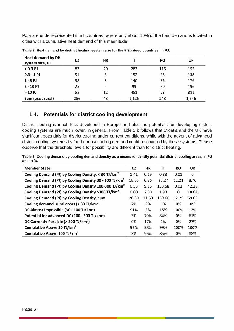
Page 6
PJ/a are underrepresented in all countries, where only about 10% of the heat demand is located in
cities with a cumulative heat demand of this magnitude.
Table 2: Heat demand by district heating system size for the 5 Stratego countries, in PJ.
Heat demand by DH system size, PJ
CZ HR IT RO UK
< 0.3 PJ 87 20 283 116 155
0.3 - 1 PJ 51 8 152 38 138
1 - 3 PJ 38 8 140 36 176
3 - 10 PJ 25 - 99 30 196
> 10 PJ 55 12 451 28 881
Sum (excl. rural) 256 48 1,125 248 1,546
1.4. Potentials for district cooling development
District cooling is much less developed in Europe and also the potentials for developing district
cooling systems are much lower, in general. From Table 3 it follows that Croatia and the UK have
significant potentials for district cooling under current conditions, while with the advent of advanced
district cooling systems by far the most cooling demand could be covered by these systems. Please
observe that the threshold levels for possibility are different than for district heating.
Table 3: Cooling demand by cooling demand density as a means to identify potential district cooling areas, in PJ and in %.
Member State CZ HR IT RO UK
Cooling Demand (PJ) by Cooling Density, < 30 TJ/km2 1.41 0.19 0.83 0.01 0
Cooling Demand (PJ) by Cooling Density 30 - 100 TJ/km2 18.65 0.26 23.27 12.21 8.70
Cooling Demand (PJ) by Cooling Density 100-300 TJ/km2 0.53 9.16 133.58 0.03 42.28
Cooling Demand (PJ) by Cooling Density >300 TJ/km2 0.00 2.00 1.93 0 18.64
Cooling Demand (PJ) by Cooling Density, sum 20.60 11.60 159.60 12.25 69.62
Cooling demand, rural areas (< 30 TJ/km2) 7% 2% 1% 0% 0%
DC Almost Impossible (30 - 100 TJ/km2) 91% 2% 15% 100% 12%
Potential for advanced DC (100 - 300 TJ/km2) 3% 79% 84% 0% 61%
DC Currently Possible (> 300 TJ/km2) 0% 17% 1% 0% 27%
Cumulative Above 30 TJ/km2 93% 98% 99% 100% 100%
Cumulative Above 100 TJ/km2 3% 96% 85% 0% 88%

Page 7
2. Assessment of investment costs for heat and cold distribution
2.1. Background
The assignment is to estimate the average investment costs for heat and cold distribution as a
function of the heat and cold densities for modelling and planning purposes. This aim is achieved by
elaborating the basic theory of heat and cold distribution costs presented in section 11.4 of the
international textbook of (Frederiksen & Werner, 2013).
2.2. Method
The expected output from this estimation analysis is to obtain the specific investment cost for heat
and cold distribution as a function of heat and cold densities. This output is achieved in five steps:
Estimation of the investment cost per metre of trench length by pipe dimension and ground
conditions.
Estimation of the average investment cost with respect to typical ground conditions.
Estimation of the average pipe dimension from the linear heat density
Estimation of the average investment cost from the average pipe dimension as a function of
the land area density as heat or cold demand per land area
Final estimation of the specific investment cost per heat and cold sold as a function of the
heat and cold densities.
2.3. Intermediate estimations
The two first two steps are presented in Figure 2, showing the investment cost for district heating
pipes per trench length. The information is based on the Swedish cost level of 2007. Hereby, the
cost level includes also a learning process for putting the pipes efficiently into the ground as achieved
in mature district heating countries. Small pipes are normally used in areas with single family areas,
with a high proportion of green areas. Wider pipes are normally used in inner city areas with higher
building densities and higher construction costs, as presented in Figure 2. These ground conditions
are considered when creating the average cost line by using the marked dots in Figure 2. This
estimated linear average cost line will have the following composition:
Average investment cost = 130 + 2858*(average pipe diameter in m) [EUR/m]
The third step will utilize the experienced relation between the linear heat densities and the average
pipe dimensions in 134 Swedish heat distribution networks or parts of networks as presented in
Figure 11.8 in (Frederiksen & Werner, 2013). The linear heat density is the heat sold annually divided
by the corresponding trench length. This relation can be written as
Average pipe dimension = 0.0486 * LN (linear heat density in MWh/m) + 0.063 [m]
The fourth step is obtained by combining the average cost line in Figure 2, the relation above for the
average pipe dimension, and an effective width of 65 m. The latter assumption for the effective width
is based on Figure 11.10 in (Frederiksen & Werner, 2013) showing that the effective width is almost
constant at that level for plot ratios above 0.4. The effective width is needed since the linear densities
are equal to the product of the effective width and the land area densities. The intermediate result
from the fourth step is presented in Figure 3.

Page 8
Figure 2: The investment cost for distribution pipes per trench length by pipe dimension and ground conditions
based on Swedish experiences for the 2007 cost level.
Figure 3: The estimated average distribution costs for district heating and district cooling as a function of the
heat and cold densities, respectively.
The average cost line for district cooling was estimated with pipe dimensions that are wider than the
corresponding pipe dimension for district heating. The used upscaling factor was the square root of
five, since the flows in district cooling networks are about five times higher than in district heating

Page 9
networks at same demand levels. This higher flow level appear since the temperature differences in
district cooling networks are about one fifth of the temperature differences in district heating
networks.
2.4. Result
The final fifth and resulting step in the estimation is presented in Figure 3. The specific average
investment costs were estimated by dividing the average investment costs in Figure 2 by the
corresponding linear densities as defined in (Frederiksen & Werner, 2013). The linear densities were
again estimated by the product of the land area densities with the assumed constant effective width
of 65 m.
These specific average investment costs are consequentially being used within the STRATEGO
project for overall assessments and feasibility studies for new or extended district heating and district
cooling networks.
Figure 4. The specific investment cost per heat or cold annually sold as function of the heat and cold densities, both related to the corresponding land area.
From Figure 4 it follows that district cooling systems are more expensive to install for the same
amount of energy delivered. The highest sensitivity to energy density is in the low density areas at
the threshold to economic feasibility. It can be expected that the geographical boundaries between
collective and individual heating or cooling systems are subject to high cost sensitivity also, as the
cost curves suggest.

Page 10
2.5. Cost-supply analysis
In cost-supply analysis, the marginal costs of cumulative utilization of a potential are given. A cost-
supply curve establishes a mathematical relation between the amount of a given resource (in this
case heating or cooling demand) and their costs (here the annualized investment costs to utilize the
resource). The basic assumption is that the most economical portions of a resource are used first,
to be followed by marginally less attractive, in economic terms. Cost-supply curves of district heating
and cooling therefor allow for establishing the costs of supply especially for supply, whose cost highly
depends on the potentials used. Because the potentials of district energy highly depend on the
location, distribution and distance to sources, it is obvious to use GIS-based cost-supply modelling.
The inputs to this are a) the quantification of costs, b) the quantification of supply available at these
costs, and c) several other attributes to be used to further specify the cost-supply relations, such as
member state, size of system, or the availability of renewable energy sources. All these data can be
retrieved from the Heating and Cooling Atlas.
Investment costs have been annualized using a technical lifetime of 30 years and a socio-economic
interest rate of 3%.
Figure 5 shows the cost-supply curves for the five countries participating in work package 2 of the
Stratego-project as per cent of total urban heat demand. In the UK, the Czech Republic and in Italy
about 25% of the total demand in villages, towns and cities can be supplied at less than 1.5 €/GJ
annual heat demand. At a threshold of 2 €/GJ the share rises to 50 – 70% in these countries, which
is well consistent with Persson and Werner (2011). For Romania the costs are on a higher level
because of the low demand densities, while in Croatia the cost-supply curve in Figure 5 is very steep
initially and the costs are generally very high, while the economic potential is very small for both
countries. Generally, the steeper the cost curves, the higher i the cost sensitivity to geographical
factors. It has to be added that the feasibility also depends on the costs of heat supply, and that the
specific investment costs are here assumed to be the same for all countries despite different levels
of labour costs etc.

Page 11
Figure 5: Cost-supply curves for district heat distribution for the 5 STRATEGO countries showing the average, annualized costs of developing district heating distribution infrastructure.
Costs of distributing district cooling are generally higher, partly because the higher specific costs but
also because of generally lower cooling demand densities; see Figure 6. At a threshold of 2€/GJ
(annualized) the UK may have 22% of its potential cooling demand covered with district cooling,
while Croatia may just be at 3% and the other Stratego countries are left with minute potentials at
this level. At 2.5 €/GJ, Italy reaches 4%, Croatia 44%, and the UK 56%. Italy reaches 42% at 3€/GJ,
while the economic potential remains zero in the Czech Republic and in Romania. However, one
great uncertainty is the degree of connectedness of the cooling demand in towns and cities, which
along with the fact that all above figures relate to the potential cooling demand, makes any results
uncertain and indicative only.
-
1.00
2.00
3.00
4.00
5.00
6.00
0% 10% 20% 30% 40% 50% 60% 70% 80% 90% 100%
Ave
rage
an
nu
aliz
ed c
ost
s o
f D
H d
istr
ibu
tio
n
inve
stm
en
ts [
€/G
J]
Cumulative utilisation of DH potential
CZ HR IT RO UK

Page 12
Figure 6: Cost-supply analysis of district cooling grids showing average annualised costs of establishing DC grids in the five Stratego countries.
DH potential by size of system
Using the prospective supply system properties, cost-supply curves can be produced for different
system types as well. Accordingly, Figure 7 presents a cost-supply curve for the Czech Republic by
prospective district heating system size. Each curve features a more or less distinct turn at which
costs increase disproportionally. This indicates a point where the economic (under most optimistic
conditions) and the total potential can be separated. Usually the economic potential, it follows from
this example, is about half of the total. Depending on the threshold for economic feasibility, which is
subject to an overall economic assessment, because other cost factors, such as the production costs
of district heat, need to be included, the economic potential for a given location and system size can
be derived for systems of different size. It can be seen that larger systems, because they are usually
located in denser urban areas of bigger towns and cities, have lower distribution costs than smaller
systems. It shows that in the Czech Republic systems > 10PJ/a have a heat supply market of 38PJ/a
at an annualized distribution cost of 1.5€/GJ, while another 10PJ/a can be found in systems of 1-3
and 3-10 PJ/a, respectively. For smaller systems the steeper curves furthermore indicate greater
uncertainties in the economic potentials.
The economic potentials for district heating in Croatia require generally higher investments in
distribution grid infrastructure. Assuming cost thresholds of 2.5 €/GJ, the biggest systems may
realize 5PJ/a, while another 3PJ is available in smaller systems, see Figure 8.
-
1.00
2.00
3.00
4.00
5.00
6.00
7.00
8.00
0% 10% 20% 30% 40% 50% 60% 70% 80% 90% 100%
Ave
rage
an
nu
alis
ed
co
sts
of
DC
dis
trib
uti
on
inve
stm
en
ts
[€/G
J]
Cumulative utilization of DC potentiall
CZ HR IT RO UK

Page 13
Italy shows good economic potentials for the development of district heating systems, see Figure 9.
At 2 €/GJ, almost all of the heat demand in the largest cities can be covered, while the share is 50-
70% for systems between 0.5 and 10 PJ. Even the smallest systems < 0.3 PJ/a may represent a
potential market.
Romania, because it is predominantly rural, has a rather small district heating potential. However,
almost all of the heat demand in the biggest city of Bucharest can be covered by district heating, as
well as the major part in systems between 1 and 10 PJ annual demand, see Figure 10.
Finally, the heat market of the UK is greatly dominated by large cities, which comprise 80% of the
economic potential at 1.5 €/GJ annualized costs, see Figure 11.
Figure 7: The cost-supply curve for district heating potentials in the Czech Republic by prospective district
heating system size.
-
0.50
1.00
1.50
2.00
2.50
3.00
3.50
4.00
4.50
5.00
- 20 40 60 80 100 120
An
nu
aliz
ed a
vera
ge d
istr
ibu
tio
n c
ost
s [€
/GJ]
Cumulative heat demand [PJ]
CZ > 10PJ/a CZ 3-10 PJ/a CZ 1-3 PJ/a CZ 0.5-1 PJ/a CZ < 0.5 PJ/a

Page 14
Figure 8: Cost-supply curve for district hearting potentials in Croatia by prospective district heating system size.
Figure 9: Cost-supply curves for district heating potentials in Italy by prospective district heating system size.
-
1.00
2.00
3.00
4.00
5.00
6.00
7.00
8.00
- 5 10 15 20 25
An
nu
aliz
ed d
istr
ibu
tio
n c
ost
s [€
/GJ
he
at d
em
and
]
Cumulative heat demand [PJ]
HR > 10PJ/a HR 3-10 PJ/a HR 1-3 PJ/a HR 0.5-1 PJ/a HR < 0.5 PJ/a
-
0.50
1.00
1.50
2.00
2.50
3.00
3.50
- 50 100 150 200 250 300 350 400 450 500
An
nu
aliz
ed d
istr
ibu
tio
n c
ost
s [€
/GJ
he
at d
em
and
]
Cumulative heat demand [PJ]
IT > 10PJ/a IT 3-10 PJ/a IT 1-3 PJ/a IT 0.5-1 PJ/a IT < 0.5 PJ/a

Page 15
Figure 10: Cost-supply curves for district heating potentials in Romania by prospective district heating system
size.
Figure 11: Cost-supply curves for district heating potentials in the United Kingdom by prospective district
heating system size.
-
1.00
2.00
3.00
4.00
5.00
6.00
7.00
8.00
9.00
- 20 40 60 80 100 120 140
An
nu
aliz
ed d
istr
ibu
tio
n c
ost
s [€
/GJ
he
at d
em
and
]
Cumulative heat demand [PJ]
RO > 10PJ/a RO 3-10 PJ/a RO 1-3 PJ/a RO 0.5-1 PJ/a RO < 0.5 PJ/a
-
0.50
1.00
1.50
2.00
2.50
3.00
3.50
- 100 200 300 400 500 600 700 800 900 1,000
An
nu
aliz
ed d
istr
ibu
tio
n c
ost
s [€
/GJ
he
at d
em
and
]
Cumulative heat demand [PJ]
UK > 10PJ/a UK 3-10 PJ/a UK 1-3 PJ/a UK 0.5-1 PJ/a UK < 0.5 PJ/a

Page 16
References
Frederiksen S and Werner S, District Heating and Cooling. Studentlitteratur, 2013.
Persson U, Werner S, Heat distribution and the future competitiveness of district heating. Applied
Energy 88 (2011) 568-576.