Quantifyin g the Net Social Ben efits of ehicle Trip Redu … accident reductions, congestion...
77
G Quan uidanc ntifyin ce for C ng the Ve Custom 42 e Net ehicle mizing t Cen University o 202 E. Fowle Socia Trip the TR Contract nter for Urba of South Flor r Ave., CUT1 al Ben Redu RIMMS© Final D t No. BD549, W FDOT P Rep an Transport rida, College 100, Tampa, efits o ctions © Mod Draft Repo Work Order # April, 20 Project Manag Amy D ort prepared Sisinnio Con Philip L. Wint tation Resea e of Engineer FL 33620‐53 of s: el ort #52 009 ger: Datz d by: ncas ters arch ring 375
-
Upload
trinhnguyet -
Category
Documents
-
view
214 -
download
1
Transcript of Quantifyin g the Net Social Ben efits of ehicle Trip Redu … accident reductions, congestion...

G
Quan
uidanc
ntifyin
ce for C
ng theVe
Custom
42
e Net ehicle mizing t
Cen
University o
202 E. Fowle
Socia Trip the TR
Contract
nter for Urba
of South Flor
r Ave., CUT1
al Ben ReduRIMMS©
Final D
t No. BD549, W
FDOT P
Rep
an Transport
rida, College
100, Tampa,
efits octions© Mod
Draft Repo
Work Order #
April, 20
Project Manag
Amy D
ort prepared
Sisinnio Con
Philip L. Wint
tation Resea
e of Engineer
FL 33620‐53
of s: el
ort
#52
009
ger:
Datz
d by:
ncas
ters
arch
ring
375

iiQuantifying the Net Social Benefits of Vehicle Trip Reductions: Guidance for Customizing the TRIMMS Model
This research was conducted under a grant from the Florida Department of Transportation. The opinions, findings, and conclusions expressed in this report are those of the authors and not necessarily those of the Florida Department of Transportation.

iiiQuantifying the Net Social Benefits of Vehicle Trip Reductions: Guidance for Customizing the TRIMMS Model
Technical Report Documentation Page
1. Report No. BD 549 WO 52
2. Government Accession No.
3. Recipient's Catalog No.
4. Title and Subtitle Quantifying the Net Social Benefits of Vehicle Trip Reductions: Guidance for Customizing the TRIMMS© Model
5. Report Date April, 2009
6. Performing Organization Code
7. Author(s) Concas, Sisinnio, Winters, Philip L.
8. Performing Organization Report No. 77805
9. Performing Organization Name and Address National Center for Transit Research Center for Urban Transportation Research University of South Florida 4202 E. Fowler Ave., CUT 100 Tampa, FL 33620‐5375
10. Work Unit No. (TRAIS)
11. Contract or Grant No. BD 549 WO 52
12. Sponsoring Agency Name and Address Florida Department of Transportation, Office of Public Transportation Transit Planning Program Florida Department of Transportation Research Center 605 Suwannee Street, MS 30 Tallahassee FL 32399‐0450
13. Type of Report and Period Covered Final Report
01/17/08 ‐ 07/08/09
14. Sponsoring Agency Code
15. Supplementary Notes FDOT Project Manager: Amy Datz
16. Abstract This study details the development of a series of enhancements to the Trip Reduction Impacts of Mobility Management Strategies (TRIMMS) model. TRIMMS© allows quantifying the net social benefits of a wide range of transportation demand management (TDM) initiatives in terms of emission reductions, accident reductions, congestion reductions, excess fuel consumption and adverse global climate change impacts. The model also includes a sensitivity analysis module that provides program cost‐effectiveness assessment. This feature allows conducting TDM evaluation to meet the Federal Highway Administration Congestion and Air Quality (CMAQ) Improvement Program requirements for program effectiveness assessment and benchmarking. This document provides guidance to help TDM professionals to use the model by selecting the appropriate cost parameters, providing referenced sources where such parameters can be obtained, and by offering general guidance on how to incorporate data already at their disposal.
17. Key Word Transportation Demand Management, TDM, TDM Evaluation, TDM prediction models, TRIMMS©
18. Distribution Statement No restrictions
19. Security Classif. (of this report) Not classified
20. Security Classif. (of this page)
21. No. of Pages
22. Price
Form DOT F 1700.7 (8‐72) Reproduction of completed page authorized

ivQuantifying the Net Social Benefits of Vehicle Trip Reductions: Guidance for Customizing the TRIMMS Model
Acknowledgements
TBD
FDOT Project Manager
Amy Datz
Florida Department of Transportation, Office of Public Transportation
CUTR Project Team
Principal Investigator: Sisinnio Concas
Co‐Principal Investigator: Philip L. Winters
Working Group
Transportation Demand Management

vQuantifying the Net Social Benefits of Vehicle Trip Reductions: Guidance for Customizing the TRIMMS Model
Executive Summary With funding from the Florida Department of Transportation and the U.S. Department of Transportation, the National Center for Transit Research (NCTR) at the Center for Urban Transportation Research (CUTR), University of South Florida (USF), recently developed TRIMMS© (Trip Reduction Impacts for Mobility Management Strategies), a practitioner‐oriented sketch planning tool.
TRIMMS© is a spreadsheet application that estimates the impacts of a broad range of transportation demand management (TDM) initiatives and provides program cost effectiveness measures, such as net program benefits and benefit to cost ratio indicators.
TRIMMS© evaluates strategies directly affecting the cost of travel, like public transportation subsidies, parking pricing, pay‐as‐you‐go pricing and other financial incentives. TRIMMS© also evaluates the impact of strategies affecting access and travel times and a host of employer‐based program support strategies, such as flexible working hours, telecommuting and guaranteed ride home programs.
In this study, we further enhance TRIMMS© by allowing regional customization of default benefit and cost parameters. This allows a wider range of default values needed for the analysis, specifying under what conditions or ranges of conditions the values can be considered reliable or appropriate. This flexibility will improve the ability of TDM practitioners to identify and put in place TDM programs that can produce the highest estimated social benefits. Further, for agencies that want to tailor default values to their areas, the research provides sample data collection and measurement methods.
Results
The model new version, TRIMMS© 2.0 presents notable improvements. Specifically, the model now offers default parameters for 85 metropolitan statistical areas in the U.S. encompassing large and small urban areas. The model’s improvements allow improved customization and the ability to clearly differentiate between analysis at the regional and employer‐site levels.
Recognizing that there is uncertainty in the value of inputs such as cost of accidents, emissions costs, we added an extended capability to allow sensitivity analysis of the impact estimates. This feature is not present in any other currently available spreadsheet application of this kind. The simulation can help practitioners estimate the probability that program benefit‐to‐cost ratios will at least be greater than some predetermined benchmarking value. This feature allows conducting TDM evaluation to meet the Federal Highway Administration Congestion and

viQuantifying the Net Social Benefits of Vehicle Trip Reductions: Guidance for Customizing the TRIMMS Model
Air Quality (CMAQ) Improvement Program requirements for program effectiveness assessment and benchmarking.
Further Research
TRIMMS© 2.0 provides significant improvements over the earlier version. Still, there are areas where the tool could be expanded. For example, one future enhancement to TRIMMS© 2.0 could provide guidance on estimating the costs for the various TDM programs rather than treating total program costs as a single input.
• While TRIMMS© 2.0 focuses on the social benefits of TDM, the effectiveness of TDM programs depends on employer cooperation and policies supporting these strategies.
• Employees’ use of transit depends on the compatibility of the work hour policies, such as flextime. The effectiveness of advanced traveler information systems to alter arrival and departure times to avoid congested periods depends on those same employer policies.
• Employer work‐life friendly programs, such as compressed workweek programs and telework influence when or if a commute trip is made.
• Employer parking policies determine the availability and price of parking that influence mode choice by employees.
• Employer provision of bike and locker facilities can make the difference between someone choosing to drive or use a non‐motorized method.
TDM provides a variety of benefits to employers as well as society. Telework programs can improve productivity, enhance recruitment and retention of employees, and reduce absenteeism. Compressed work week programs enable the employer to expand coverage to enhance customer service. Employers allowing employees to pay for transit passes and parking as a pre‐tax benefit save payroll taxes. While most of the tools available to assess the impacts of TDM strategies focus on air quality benefits, there is a lack of tools to assist employers in assessing the costs and potential business benefits of implementing TDM programs. A return‐on‐investment approach based on these employer benefits and costs, augmented by the Monte Carlo analysis, could be perceived as a very useful tool to commuter assistance programs that work with employers in establishing TDM programs at worksites.
Finally, integrating TRIMMS© 2.0 as an off‐model to be used with the four‐step regional transportation planning models could assist transportation planners in estimating the impacts on traffic flows and traffic congestion in particular corridors due to TDM. TRIMMS© 2.0 could modify the mode choice and trip generation inputs to the regional models for that purpose.

viiQuantifying the Net Social Benefits of Vehicle Trip Reductions: Guidance for Customizing the TRIMMS Model
[This page Intentionally Left Blank]

viiiQuantifying the Net Social Benefits of Vehicle Trip Reductions: Guidance for Customizing the TRIMMS Model
Table of Contents
Executive Summary ................................................................................................................. v
List of Tables............................................................................................................................ x
List of Figures .......................................................................................................................... 1
Chapter 1: Introduction ........................................................................................................... 2
1.1 Introduction ...................................................................................................................... 2
1.2 Objectives ......................................................................................................................... 3
1.3 Research Approach .......................................................................................................... 3
1.3.1 Cost and Travel Time Elasticity Parameters Collection and Analysis .................................... 3
1.3.2 Guidance to Update and Customization of Cost‐Benefit Parameters .................................. 4
1.3.3 TRIMMS© Model Update to Version 2.0 .............................................................................. 4
1.4 Report Organization ......................................................................................................... 4
Chapter 2: Development of TRIMMS© 2.0 .............................................................................. 5
2.1 Introduction ...................................................................................................................... 5
2.2 Overview of the TRIMMS© Model .................................................................................. 5
2.3 New Spreadsheet Layout ................................................................................................. 8
2.3.1 Step 1 – Analysis Description and Scope .............................................................................. 9
2.3.2 Step 2 – Geographical Area Selection ................................................................................... 9
2.3.2 Step 3 – Program Details ..................................................................................................... 11
2.3.3 Step 4 – Baseline Mode Shares and Trip Length ................................................................. 13
2.3.4 Step 5 through 9 – Employer Support Program Evaluation ................................................ 14
2.3.5 Step 10 – Financial and Pricing Strategies Evaluation......................................................... 18
2.3.6 Step 11 – Access and Travel Time Improvements Evaluation ............................................ 18
2.3.7 Output ................................................................................................................................. 19
2.4 Impact Analysis Disaggregation ..................................................................................... 20
2.4.1 Changes in Air Pollution Emissions Costs ............................................................................ 21
2.4.2 Changes in Congestion Costs .............................................................................................. 21
2.4.3 Changes in Excess Fuel Consumption Costs ........................................................................ 22
2.4.4 Changes in Global Climate Change Costs ............................................................................ 22
2.4.5 Changes in Health and Safety Costs .................................................................................... 22

ixQuantifying the Net Social Benefits of Vehicle Trip Reductions: Guidance for Customizing the TRIMMS Model
2.4.6 Changes in Noise Pollution Cost ......................................................................................... 22
2.5 Default Input Disaggregation ......................................................................................... 23
2.6 Sensitivity Analysis Module ............................................................................................ 23
Chapter 3: Guidance to Update Input Parameters ................................................................. 25
3.1 Introduction .................................................................................................................... 25
3.2 TRIMMS© basic input parameters ................................................................................ 25
3.2.1 Global Parameters .............................................................................................................. 25
3.2.2 Regional Parameters ........................................................................................................... 27
3.3 Estimation of External or Social Costs ............................................................................ 28
3.3.1 Congestion Costs ................................................................................................................. 28
3.3.2 Health and Safety ................................................................................................................ 31
3.3.4 Air Pollution ........................................................................................................................ 34
3.3.5 Global Climate Change ........................................................................................................ 37
3.3.6 Noise Pollution .................................................................................................................... 38
3.4 Guidance on How to Update Input Parameters ............................................................. 39
3.4.1 Global and Regional Inputs ................................................................................................. 39
3.4.2 Social Cost Parameters ........................................................................................................ 40
3.5 Trip Demand Functions Elasticity Parameters ............................................................... 43
3.5.1 Guidance on How to Update Elasticity Parameters ............................................................ 46
Chapter 4: Sensitivity Analysis Module .................................................................................. 47
4.1 Introduction .................................................................................................................... 47
4.2 Monte Carlo Simulation ................................................................................................. 47
4.3 Running TRIMMS© Sensitivity Analysis Module ........................................................... 49
Chapter 5: Conclusions .......................................................................................................... 55
5.1 Model Limitations .......................................................................................................... 55
5.2 Directions for Further Research .......................................................................................... 56
References............................................................................................................................. 58
Appendix A: Constant Elasticity Trip Demand Functions ........................................................ 60
Appendix B: List of Metropolitan Statistical Areas ................................................................. 65

xQuantifying the Net Social Benefits of Vehicle Trip Reductions: Guidance for Customizing the TRIMMS Model
List of Tables Table 3.1 Value of Time: All Occupations, 2007 dollars ............................................................... 30 Table 3.2 Monetary and Nonmonetary Crash Costs ($/crash, 2002 dollars) ............................... 32 Table 3.3 Crash Rates (crashes/million VMT) ‐ Florida ................................................................. 33 Table 3.4 Example of Parameter Regionalization ‐ NOX Health Emissions .................................. 36 Table 3.5 Noise Pollution Costs .................................................................................................... 38 Table 3.6 Fare and Price Elasticities .............................................................................................. 44 Table 3.7 Travel Time Elasticities .................................................................................................. 45 Table 3.8 Parking Pricing Elasticities ............................................................................................. 46

Quantifying the Net Social Benefits of Vehicle Trip Reductions: Guidance for Customizing the TRIMMS Model
1
List of Figures Figure 2.1 TRIMMS© Model Structure ........................................................................................... 7 Figure 2.2 TRIMMS© – Introduction .............................................................................................. 8 Figure 2.3 TRIMMS© – Step 1 – Analysis Description and Scope ................................................ 10 Figure 2.4 TRIMMS© – Step 2 – Geographic Area Selection ........................................................ 10 Figure 2.5 TRIMMS© – Step 3 – Program Information: Employer Based Analysis ...................... 12 Figure 2.6 TRIMMS© – Step 3 –Program Information: Area Wide Analysis ................................ 12 Figure 2.7 TRIMMS© – Step 4 – Mode Share and Trip Length..................................................... 13 Figure 2.8 TRIMMS© – Step 5 – Program Support Evaluation: Program Subsidies ..................... 14 Figure 2.9 TRIMMS© – Program Support Evaluation: GRH and Ride Match ............................... 15 Figure 2.10 TRIMMS© – Program Support Evaluation: Telework and Flex Hours ....................... 15 Figure 2.11 TRIMMS© – Program Support Evaluation: Worksite Accessibility ........................... 16 Figure 2.12 TRIMMS© – Program Support Evaluation: Worksite Amenities ............................... 16 Figure 2.13 TRIMMS© – Program Support Evaluation: Worksite Parking ................................... 17 Figure 2.14 TRIMMS© – Program Support Evaluation: Program Marketing ............................... 17 Figure 2.15 TRIMMS© – Step 10 – Financial and Pricing Strategies ............................................ 18 Figure 2.16 TRIMMS© – Step 11 – Access and Travel Time Improvements Evaluation .............. 19 Figure 2.17 TRIMMS© – Results Worksheet ................................................................................ 20 Figure 2.18 TRIMMS© – Air Pollution Estimates .......................................................................... 21 Figure 3.1 Model Parameters Module: Global Parameters .......................................................... 39 Figure 3.2 Model Parameters Module: Regional Parameters ...................................................... 40 Figure 3.3 Model Parameters Module: Air Pollution Costs .......................................................... 41 Figure 3.4 Model Parameters Module: Congestion Costs ............................................................ 41 Figure 3.5 Model Parameters Module: Global Climate Change Costs ......................................... 42 Figure 3.6 Model Parameters Module: Health and Safety Costs ................................................. 42 Figure 3.7 Model Parameters Module: Noise Pollution Costs...................................................... 43 Figure 3.8 Elasticities Worksheet .................................................................................................. 46 Figure 4.1 Monte Carlo Simulation Example: Changes in Fuel Consumption Costs ..................... 49 Figure 4.2 Summary of TDM Costs and Benefits taken from Results Sheet ................................. 50 Figure 4.3 Sensitivity Analysis Prompt Screen .............................................................................. 51 Figure 4.4 MC Simulation Progress Status Bar ............................................................................. 52 Figure 4.5 TRIMMS© Sensitivity Analysis Results ........................................................................ 52 Figure 4.6 Sensitivity Analysis with B/C target set at 2.0 ............................................................. 53 Figure 4.7 Sensitivity Analysis Results with B/C target set at 2.0 ................................................. 54

Quantifying the Net Social Benefits of Vehicle Trip Reductions: Guidance for Customizing the TRIMMS Model
2
Chapter 1: Introduction
1.1 Introduction
The Federal Highway Administration Congestion and Air Quality CMAQ) Improvement Program provides explicit guidelines to program effectiveness assessment and benchmarking. The program calls for quantitative analysis of benefits and disbenefits (i.e., emission increases) resulting from emission reduction strategies for project selection of congestion and emission reduction initiatives [1]. In a partial attempt to quantify the net social benefits of congestion reduction strategies, an increasing number of state, regional, and local agencies are attempting to measure the benefits of transportation demand management (TDM) initiatives. Transportation Demand Management or TDM (also called Mobility Management) refers to various strategies that change travel behavior to increase transport system efficiency and achieve specific planning objectives [2]. .
With funding from the Florida Department of Transportation and the US Department of Transportation, the National Center for Transit Research at the University of South Florida recently developed the TRIMMS© (Trip Reduction Impacts for Mobility Management Strategies) model [3]. TRIMMS© is a visual basic (VB) application spreadsheet model that estimates the impacts of a broad range of TDM initiatives and provides program cost effectiveness measures, such as net program benefits and benefit‐to‐cost ratio analysis.
TRIMMS© evaluates strategies directly affecting the cost of travel, like public transportation subsidies, parking pricing, pay‐as‐you‐go pricing initiatives and other financial incentives. TRIMMS© also evaluates the impact of strategies affecting access and travel times and a host of employer‐based program support strategies, such as flexible working hours, telecommuting and guaranteed ride home programs. TRIMMS© permits program managers and funding agencies like FDOT to make informed decisions on where to spend finite transportation dollars based on a full range of benefits and costs. The model allows some regions to use local data or opt to use defaults from national research findings, select the benefits and costs of interest, and calculate the costs and benefits of a given program.
In this study, we further enhance TRIMMS© by allowing regional customization of default benefit and cost parameters. The enhancement allows a wider range of default values needed for the analysis, specifying under what conditions the values can be considered reliable or appropriate. This will improve the ability of TDM practitioners to identify and put in place TDM programs that can produce the highest estimated social benefits. TRIMMS© also applies an economic analysis approach comparable to those used for infrastructure investment

Quantifying the Net Social Benefits of Vehicle Trip Reductions: Guidance for Customizing the TRIMMS Model
3
evaluation. Furthermore, this research provides sample data collection and measurement methods to guide agencies that want to tailor default values to their areas.
1.2 Objectives
The objective of this study is twofold. First, we collect a broad range of cost and benefit parameters to allow model customization at a regional level. In addition to this data collection effort, we update the model to a new, streamlined, version. Second, this project provides the research and documentation necessary to help professionals to use the model by selecting the appropriate cost parameters, with clear reference to the sources where such parameters can be obtained, and by offering general guidance on how to incorporate data already at their disposal.
1.3 Research Approach
The current version of TRIMMS© makes use of cost‐benefit parameters culled from a literature review of benefits and impact of TDM initiatives at the national level. Although the model allows updating these parameters, it does not differentiate between regional areas across the U.S. We updated the parameters to take into account differences that exist between geographical areas in terms of congestion emission rates, costs, and population density levels. Finally, we implemented a series of enhancements that update TRIMMS© to a new version. We detail these improvements in this report.
1.3.1 Cost and Travel Time Elasticity Parameters Collection and Analysis
At the core of TRIMMS© is the capability to estimate mode share changes. The modeling framework allows capturing a broader range of trade‐offs that users constantly face and is capable of quantifying impacts on travel patterns by using prices as the direct drivers of travel demand. Furthermore, the approach is able to take into account how individuals re‐adjust over time in their trade‐offs. The estimation of modal share changes brought about by TDM strategies affecting the generalized time and monetary costs of travel are based on specific trip demand functions. These functions rely on cost and travel time elasticity parameters.
The objective of this task is to revisit each trip demand function to incorporate additional elasticities that estimate a broader range of impacts. For example, the transit travel demand function will be expanded to account for the different impact a fare change exerts, depending on time of the day (peak and off‐peak).

Quantifying the Net Social Benefits of Vehicle Trip Reductions: Guidance for Customizing the TRIMMS Model
4
1.3.2 Guidance to Update and Customization of CostBenefit Parameters
The objective of this task is to produce a technical document to help professionals to use the model and the cost parameters, and to provide a reference to sources where such parameters can be obtained.
1.3.3 TRIMMS© Model Update to Version 2.0
One of the project tasks was updating the TRIMMS© model to allow more customization, and to clearly differentiate between analysis at the regional and employer‐site levels. Furthermore, the module that evaluates the impact of employer support programs is revised. This includes a refinement of the employer support program evaluation module, which employs parameters estimated by a panel data regression analysis of commuter trip reduction programs.
Recognizing that there is uncertainty in the value of inputs such as cost of accidents, emissions costs, we added an extended capability to allow for Monte Carlo simulation of the impact estimates. The simulation approach uses repeated random sampling to compute their results to produce a range of probable outcomes. Monte Carlo simulation uses random sampling from probability distribution functions as model inputs to produce a sensitivity analysis. As part of this update, we developed a specific algorithm that generates random variation in the input parameters. The algorithm is run many times (from a few hundred up to millions) to provide simulated ranges for the input parameters and assess which factors might be responsible for variability and uncertainty in the model outcome. This effort resulted in the design of a module that permits sensitivity analysis, a feature to date not present in any other spreadsheet application of this kind. Chapter 4 will discuss this module in more detail.
1.4 Report Organization
Chapter 2 presents and overview of TRIMMS© and describes Version 2.0. Chapter 3 goes into detail on the model’s parameters and provides guidance and sources on how to substitute default parameters with custom parameters. Chapter 4 describes the sensitivity analysis module and provides a hands‐on example on how to conduct such analysis. Chapter 5 concludes and provides direction for further research.
Quantifying the Net Social Benefits of Vehicle Trip Reductions: Guidance for Customizing the TRIMMS Model
5
Chapter 2: Development of TRIMMS© 2.0
2.1 Introduction
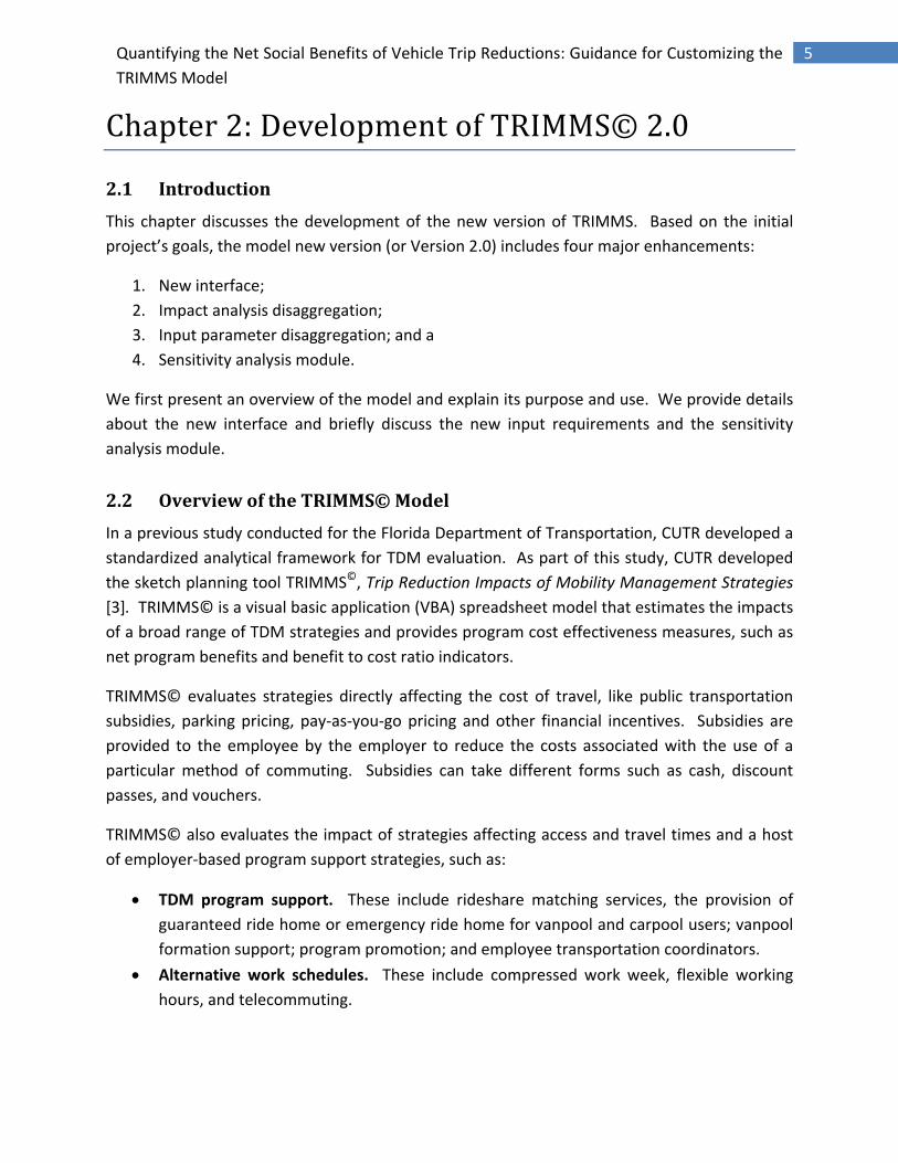
This chapter discusses the development of the new version of TRIMMS. Based on the initial project’s goals, the model new version (or Version 2.0) includes four major enhancements:
1. New interface; 2. Impact analysis disaggregation; 3. Input parameter disaggregation; and a 4. Sensitivity analysis module.
We first present an overview of the model and explain its purpose and use. We provide details about the new interface and briefly discuss the new input requirements and the sensitivity analysis module.
2.2 Overview of the TRIMMS© Model
In a previous study conducted for the Florida Department of Transportation, CUTR developed a standardized analytical framework for TDM evaluation. As part of this study, CUTR developed the sketch planning tool TRIMMS©, Trip Reduction Impacts of Mobility Management Strategies [3]. TRIMMS© is a visual basic application (VBA) spreadsheet model that estimates the impacts of a broad range of TDM strategies and provides program cost effectiveness measures, such as net program benefits and benefit to cost ratio indicators.
TRIMMS© evaluates strategies directly affecting the cost of travel, like public transportation subsidies, parking pricing, pay‐as‐you‐go pricing and other financial incentives. Subsidies are provided to the employee by the employer to reduce the costs associated with the use of a particular method of commuting. Subsidies can take different forms such as cash, discount passes, and vouchers.
TRIMMS© also evaluates the impact of strategies affecting access and travel times and a host of employer‐based program support strategies, such as:
• TDM program support. These include rideshare matching services, the provision of guaranteed ride home or emergency ride home for vanpool and carpool users; vanpool formation support; program promotion; and employee transportation coordinators.
• Alternative work schedules. These include compressed work week, flexible working hours, and telecommuting.

Quantifying the Net Social Benefits of Vehicle Trip Reductions: Guidance for Customizing the TRIMMS Model
6
• Worksite TDM oriented amenities. These include the provision of childcare facilities and the presence of sidewalks connecting transit stops within or nearby the worksite.
TRIMMS© predicts mode share and VMT changes brought about by the above TDM initiatives using constant elasticity trip demand functions. These functions estimate changes from baseline trip demands taking into account users’ responsiveness to changes in pricing and travel times. The evaluation of program support strategies is based on regression equation coefficients that weight in the relative strength of program support strategies and pricing strategies. Appendix A details the modeling technique and the use of these demand functions.
Figure 2.1 shows TRIMMS’ structure. Starting from a baseline scenario describing a TDM program in terms of commuter travel behavior (mode shares, average trip lengths, peak and off‐peak spreads), TRIMMS© evaluates the impacts of TDM implementation by estimating changes in travel behavior (mode shares, VMT reductions). Changes in the baseline scenario are then used to estimate changes in the external costs associated with these travel behavior changes.
Generally, costs that are borne directly by transportation users are defined as internal costs and those costs that are not directly borne by these users are defined as external costs. External or societal costs belong to what economists describe as negative externalities. Negative externalities arise whenever costs associated with single occupant vehicle (SOV) use, such as added congestion delay, air pollution, and increased accident risk, are not directly sustained by auto users but are rather imposed on the society as a whole. TRIMMS© estimates changes in external costs for the following externalities:
• Air pollution emissions
• Added congestion
• Excess fuel consumption
• Global climate change
• Health and safety
• Noise pollution
Chapter 3 discusses these costs, their definition and measurement.

Quantifying the Net Social Benefits of Vehicle Trip Reductions: Guidance for Customizing the TRIMMS Model
7
Figure 2.1 TRIMMS© Model Structure
Baseline CaseProgram Description ‐ Mode Shares ‐ Trip Length
Pricing and Travel Time ImpactsTrip Demand Estimation ‐ Constant Elasticity Demands
Support Program Impacts Fixed‐effect Regression Equation
Change in Baseline Case ‐ Mode Trips ‐ Mode Shares
Changes in Social Costs: ‐ Air Pollution ‐ Congestion ‐ Excess Fuel Consumption ‐ Global Climate Change ‐ Health and Safety ‐ Noise Pollution
Program Evaluation ‐ Program Annual Benefits ‐ Program Annualize Costs ‐ Net Program Benefits ‐ Benefit/Cost Ratio

Quantifying the Net Social Benefits of Vehicle Trip Reductions: Guidance for Customizing the TRIMMS Model
8
Analysts consider reductions in these cost externalities as benefits generated by TDM. TRIMMS© sums these benefits and annualizes them. It also annualizes the cost of the program and, by taking the ratio of benefits to costs, it estimates the benefit to cost (B/C) ratio. The B/C ratio is suitable for comparison across different competing TDM alternatives and for their cost‐effectiveness benchmarking with respect to the more traditional capital infrastructure investments.
2.3 New Spreadsheet Layout
The new spreadsheet layout reduces the number of steps required to conduct program evaluation and accommodates the expanded disaggregation of the model parameters. Impact analysis now makes use of default parameters tailored to 85 metropolitan statistical areas (MSAs) across the U.S. To corroborate the analysis results, we developed a new module that assesses the sensitivity of results with respect to the inputs used.
As in the previous version, the model runs on the Microsoft Excel© software platform (compatible with Excel 2007 version). As an added advantage, the new version is relatively small in size (less than one megabyte in size), which makes it easy to download and run. Upon launching the program, a welcome screen appears, the model loads up and activates a worksheet called Introduction containing the Run Analysis and User Manual button.
Figure 2.2 TRIMMS© – Introduction

Quantifying the Net Social Benefits of Vehicle Trip Reductions: Guidance for Customizing the TRIMMS Model
9
By clicking on the Run Analysis button, the model launches a module consisting of 11 steps leading to the evaluation of pricing strategies, public transit access and travel time improvements, and employer‐based support programs. At the bottom right side of the module a clickable question mark launches a help file providing a description of the purpose and function of each step.
2.3.1 Step 1 – Analysis Description and Scope
In this first step, the user enters information that identifies the analysis scenario. Upon entering the analysis date, the model immediately updates all input cost parameters to the year the analysis is being conducted. Next, the user specifies the analysis scope by either choosing area wide or site‐specific analysis. Area wide or multi‐employer analysis defines a scope where the number of travelers being affected by the policy under evaluation is represented by the total regional employment population or a specific target population. Site specific or single employer analysis allows evaluating TDM initiative for a single employment site.
The area wide option was not offered in the first version of TRIMMS© and is the result of feedback comments from users that needed to conduct a regional evaluation of various TDM programs. While the TDM initiatives that can be evaluated are the same for both options, the input requirements change. As described in the next section, area wide analysis requires basic information on the number of employers operating in the area, such as average employer size by major industrial sector. The model automatically calls these inputs after the selection of the geographical area.
2.3.2 Step 2 – Geographical Area Selection
In this step, the user selects the geographical area that most closely matches the analysis impact area. This action calls default cost and travel behavior parameters tailored for 85 metropolitan statistical areas. To customize emission factors the user can select summer or winter emission conditions and can also select if program or policy will likely affect freeway, arterial or all travel conditions. For example, the user interested in evaluating a TDM program located in the Tampa Bay region, Florida, must click on the U.S. Census region and then select the Tampa‐Saint Petersburg‐Clearwater MSA. The full list of MSA is available in Appendix B.

Quantifying the Net Social Benefits of Vehicle Trip Reductions: Guidance for Customizing the TRIMMS Model
10
Figure 2.3 TRIMMS© – Step 1 – Analysis Description and Scope
Figure 2.4 TRIMMS© – Step 2 – Geographic Area Selection

Quantifying the Net Social Benefits of Vehicle Trip Reductions: Guidance for Customizing the TRIMMS Model
11
2.3.2 Step 3 – Program Details
In this third step, the user enters specific information on the program characteristics. The information and options that can be checked change according to the scope of analysis. The model displays a different module depending on the scope of analysis selected in Step 1, as shown in Figure 4 and Figure 5. The user must enter information related to the program size, overall cost and duration. Information on the current discount rate allows annualizing program costs. The default discount rate is automatically loaded and the user can change its value in this window.
The total number of employees defines the size of the commuting population under study and is used to compute baseline vehicle trips, VMT and emissions. Depending on the scope of analysis, this figure can represent the size of a single employment site, the total regional employment population, or a specific target population. For example, if running an area wide analysis, employers below a certain size might not be required to participate in any voluntary trip reduction program. Therefore, users might want to restrict the analysis to employers of a relevant size.
Employer support programs tend to differ in terms of magnitude based on industry sector and size. If conducting a site‐based analysis (Figure 4), the user must determine the employer’s industry sector. This choice is mutually exclusive (i.e., no more than one sector can be selected at the same time). This tailors specific inputs such as the prevailing wage rate used to compute congestion cost changes and the calculation of employer support programs impacts. Employer support programs tend to differ in terms of magnitude based on the employment sector and size.
If running an area wide analysis, the user can check the industry sectors that are likely to be affected by the program. Two or more sectors can be checked. If the policy affects all sectors, then the user can check the All Sectors box. This action is relevant as it calls the geographic area default industry composition information from TRIMMS© database file and affects the calculation of baseline mode share changes.

Quantifying the Net Social Benefits of Vehicle Trip Reductions: Guidance for Customizing the TRIMMS Model
12
Figure 2.5 TRIMMS© – Step 3 – Program Information: Employer Based Analysis
Figure 2.6 TRIMMS© – Step 3 –Program Information: Area Wide Analysis

Quantifying the Net Social Benefits of Vehicle Trip Reductions: Guidance for Customizing the TRIMMS Model
13
2.3.3 Step 4 – Baseline Mode Shares and Trip Length
Based on the MSA selection, TRIMMS© calls specific default mode shares. These are obtained from the American Community Survey (ACS) three‐year average for the period 2005‐2007 and are discussed in more detail in the next chapter. If running a site specific analysis, the user enters baseline mode share information from employee travel survey data. If running an area wide analysis, then these mode shares can be used as baseline mode shares for the employment population. In the next chapter, we show how to gather this information from publicly available data for other metropolitan statistical areas not covered here.
Default average trip length is based on the National Household Travel Survey (NHTS) average trip length. Trip length differs by mode, which means that mode share shifts from drive alone to other modes will generate different VMT reductions. While the user can change trip length values right on this screen, average vehicle occupancy can be changed by clicking on the Model Parameters button on the results sheet.
The default percent of trips occurring in peak period is set at 63.9 % of all work trips. TRIMMS© uses this split to compute trip emissions for peak and off‐peak periods, recognizing that emission rates differ. The user can also change this value during this step.
Figure 2.7 TRIMMS© – Step 4 – Mode Share and Trip Length

Quantifying the Net Social Benefits of Vehicle Trip Reductions: Guidance for Customizing the TRIMMS Model
14
2.3.4 Step 5 through 9 – Employer Support Program Evaluation
Program support evaluation information is selected in five steps starting with Step 5 and ending in Step 9. The user walks through a series of screens (shown in Figure 2.8 through Figure 2.14) where several options related to employer support programs are available. This action calls specific parameters from a regression equation that predicts the mode share impacts. This action is similar the Environmental Protection Agency (EPA) COMMUTER model mode share balancing based on relational factors. The main difference is that TRIMMS© does not use relational factors based on less subjective rules of thumb about the efficacy and intensity of TDM support programs. Rather it uses coefficients estimated from a fixed effect equation that the authors run on a commute trip reduction program of Washington State running over the course of three years. We describe the statistical technique and the estimation equation in Appendix A.
Figure 2.8 TRIMMS© – Step 5 – Program Support Evaluation: Program Subsidies

Quantifying the Net Social Benefits of Vehicle Trip Reductions: Guidance for Customizing the TRIMMS Model
15
Figure 2.9 TRIMMS© – Program Support Evaluation: GRH and Ride Match
Figure 2.10 TRIMMS© – Program Support Evaluation: Telework and Flex Hours

Quantifying the Net Social Benefits of Vehicle Trip Reductions: Guidance for Customizing the TRIMMS Model
16
Figure 2.11 TRIMMS© – Program Support Evaluation: Worksite Accessibility
Figure 2.12 TRIMMS© – Program Support Evaluation: Worksite Amenities

Quantifying the Net Social Benefits of Vehicle Trip Reductions: Guidance for Customizing the TRIMMS Model
17
Figure 2.13 TRIMMS© – Program Support Evaluation: Worksite Parking
Figure 2.14 TRIMMS© – Program Support Evaluation: Program Marketing
Quantifying the Net Social Benefits of Vehicle Trip Reductions: Guidance for Customizing the TRIMMS Model
18
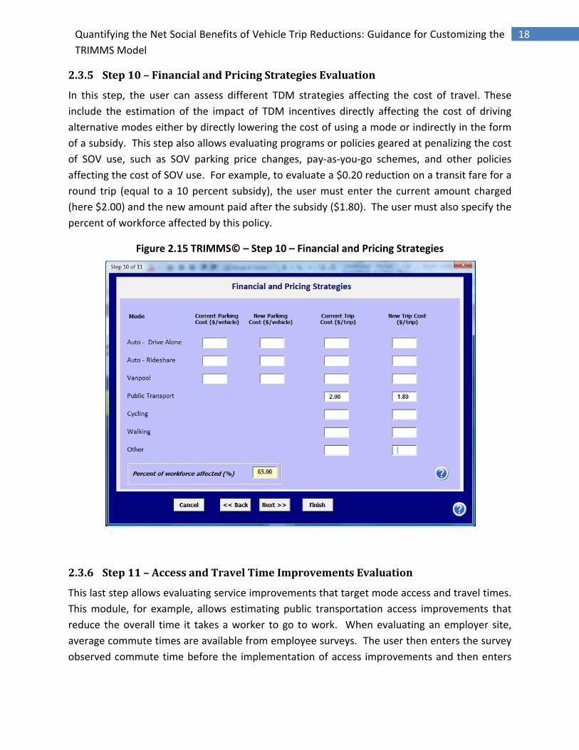
2.3.5 Step 10 – Financial and Pricing Strategies Evaluation
In this step, the user can assess different TDM strategies affecting the cost of travel. These include the estimation of the impact of TDM incentives directly affecting the cost of driving alternative modes either by directly lowering the cost of using a mode or indirectly in the form of a subsidy. This step also allows evaluating programs or policies geared at penalizing the cost of SOV use, such as SOV parking price changes, pay‐as‐you‐go schemes, and other policies affecting the cost of SOV use. For example, to evaluate a $0.20 reduction on a transit fare for a round trip (equal to a 10 percent subsidy), the user must enter the current amount charged (here $2.00) and the new amount paid after the subsidy ($1.80). The user must also specify the percent of workforce affected by this policy.
Figure 2.15 TRIMMS© – Step 10 – Financial and Pricing Strategies
2.3.6 Step 11 – Access and Travel Time Improvements Evaluation
This last step allows evaluating service improvements that target mode access and travel times. This module, for example, allows estimating public transportation access improvements that reduce the overall time it takes a worker to go to work. When evaluating an employer site, average commute times are available from employee surveys. The user then enters the survey observed commute time before the implementation of access improvements and then enters

Quantifying the Net Social Benefits of Vehicle Trip Reductions: Guidance for Customizing the TRIMMS Model
19
the new, expected, travel time after the improvement. TRIMMS© estimates mode share changes based on these numbers.
Figure 2.16 TRIMMS© – Step 11 – Access and Travel Time Improvements Evaluation
2.3.7 Output
Upon clicking the Finish button, TRIMMS© performs all calculations and displays the Results worksheet, shown in Figure 10. This sheet reports mode share, trip and VMT changes with respect to the baseline case.
TRIMMS© reports changes in social costs generated by the TDM policy under evaluation. Changes with a negative value correspond to a reduction in social costs and, therefore, represent a benefit of TDM. These values are reported in terms of daily dollar amounts. When annualized, the sum of these benefits produces the program total annual benefits, which are also reported. Finally, the results sheet produces a B/C ratio for program evaluation purposes. In this sheet, the user can conduct additional analysis by clicking on the Sensitivity Analysis button or modify the model underlying default parameters by clicking on the Model Parameters button. Additional functions include the possibility to save and print the results, perform a total reset, and modify the trip demand elasticity parameters. We describe the use of these features in detail in the next sections of this chapter.

Quantifying the Net Social Benefits of Vehicle Trip Reductions: Guidance for Customizing the TRIMMS Model
20
Figure 2.17 TRIMMS© – Results Worksheet
2.4 Impact Analysis Disaggregation
In the previous section, we discussed that one improvement of TRIMMS© is that it can perform analysis either at the regional (area wide) level or at the individual employer site. Another enhancement to the previous TRIMMS© version is its ability to provide breakdown estimates by benefit type. TRIMMS© 1.0 only presented a single aggregate estimate of the benefits related to the TDM policy under evaluation. Several TRIMMS© users commented on the desire to present a breakdown of these benefits better to assess program effectiveness. For example some users are interested in measuring TDM by its capacity to reduce air pollution emissions, while others want to know the impact on other types of benefits, such as noise pollution reductions, or its impact in terms of global climate pollution reductions. Version 2.0 now provides estimates of changes in external or social costs associated with:
• Air pollution
• Added congestion
• Excess fuel consumption
• Global climate change
• Health and safety
• Noise pollution
As previously explained these costs are defined as external costs, or costs associated with the choice of a particular mode and that are imposed to the society. For example, pollution costs, although not directly borne by a commuter using SOV to go to work, they are imposed on all

Quantifying the Net Social Benefits of Vehicle Trip Reductions: Guidance for Customizing the TRIMMS Model
21
other individuals. These costs are used in social benefit cost analysis to compare the costs and benefits associated with a given transportation alternative. Social and external costs are also relevant to pricing and are used to compare alternative plans for efficient use of transportation systems.
2.4.1 Changes in Air Pollution Emissions Costs
Air pollution costs are costs associated with emissions produced by motor vehicle use. Motor vehicles produce various harmful emissions that have negative effect at local and global levels. Exhaust air emissions cause damage to human health, visibility, materials, agriculture and forests [4, 5]. The major source of pollutants include carbon monoxide (CO), volatile organic compounds (VOCs), nitrogen oxide (NOx), sulphur oxide (SOx), and particulate matter (PM). Mobile emissions also affect global climate as gases increase the global warming effect.
TRIMMS© estimates changes in baseline VOCs, CO, NOx, CO2 emissions both in absolute quantities (lbs/day and metric tons/day) and as percentage reduction over the baseline case. Figure 11 shows a snapshot from the Results tab summarizing the change in air pollutions by pollutant.
Figure 2.18 TRIMMS© – Air Pollution Estimates
The estimation of pollution emissions relies on emission pollution factors. Upon selecting one of the 85 geographical areas, TRIMMS© loads a set of emission files that we obtained from the EPA MOBILE6 model. The next chapter describes in detail how we obtained these factors and the methods and sources to measure air pollution costs.
2.4.2 Changes in Congestion Costs
TRIMMS© estimates the costs associated with congestion delay produced by motor vehicle use. Congestion delay is the added delay imposed to all users as an additional vehicle is introduced into the traffic stream. Any TDM initiative that removes a vehicle from the road can potentially produce benefits in terms of changes or reductions in added delay. The cost of added delay is the opportunity cost of time spent on a motor vehicle for work or non‐work related purposes; time that could be spent on other activities, such as leisure or other more work. This cost is a portion of the overall travel time costs since it only considers the portion of congestion costs generated by added delay to others.
CHANGE IN EMISSIONS (Amount, Daily) (negative value is a reduction)
Pollutant Peak Off Peak Total Peak Off Peak Total Peak Off Peak TotalVOCs ‐0.13 ‐0.11 ‐0.24 0.00 0.00 0.00 ‐0.38% ‐0.34% ‐0.72%CO ‐1.24 ‐1.14 ‐2.37 0.00 0.00 0.00 ‐0.29% ‐0.27% ‐0.56%NOX ‐0.50 ‐0.33 ‐0.83 0.00 0.00 0.00 ‐1.67% ‐1.09% ‐2.76%
CO2 ‐187.31 ‐167.54 ‐354.85 ‐0.08 ‐0.08 ‐0.16 ‐1.10% ‐0.99% ‐2.09%
lbs/day metric tons/day Percent Reduction over Baseline

Quantifying the Net Social Benefits of Vehicle Trip Reductions: Guidance for Customizing the TRIMMS Model
22
2.4.3 Changes in Excess Fuel Consumption Costs
In addition to travel time‐savings, added congestion contributes to excess fuel consumption. Research shows that TDM can contribute to reduce excess fuel consumption and thus reduce dependency from fossil fuel consumption [2, 4]. TRIMMS© estimates the reduction of excess fuel consumption generated by a given TDM initiative in total gallons per day.
2.4.4 Changes in Global Climate Change Costs
Climate change costs quantify the damage associated with climate change. The Intergovernmental Panel on Climate Change (IPCC) defines climate change as the “state of any change in climate over time, whether due to natural variability or as a result of human activity [6].” Trapped heat in the atmosphere is a major driver of global climate change. Gases that trap heat in the atmosphere are called greenhouse gases. These include carbon dioxide (CO2), methane (CH4), nitrous oxide (N2O) and fluorinated gases [7]. Motor vehicle fuel production and consumption release greenhouse gases, mainly CO2, a major contributor to global climate change. EPA estimates that represents CO2 about 30 percent of all greenhouse gas emissions [8]. There are mitigation and damage costs associated with global climate change. Damage costs are costs related to the environment, health, and reduced economic productivity.
TRIMMS© estimates the impact that single occupancy vehicle use has on climate change. It measure changes in CO2 emissions and measures the costs associated with each ton of this greenhouse gas.
2.4.5 Changes in Health and Safety Costs
Health and safety costs associated with crashes represent another relevant component of social costs. These include monetary costs, such as property and personal injury damages caused by collisions and cost avoidance activities, as well as nonmonetary costs, such as pain and loss of productivity. TRIMMS© estimates the change in comprehensive health and safety costs associated with changes in the number of vehicle crashes of the TDM initiatives under evaluation.
2.4.6 Changes in Noise Pollution Cost
Noise costs quantify the damage imposed on others from motor vehicle use. Motor vehicles produce noise from engine acceleration and vibration, from tire contact on road surfaces, from break and horn usage. Noise disrupts sleep, activities, causes stress, and negatively affects property values. Several studies analyze the impact and value of external costs associated with noise emissions. TRIMMS© use default noise costs, measured in dollars per VMT, and estimates the total change in noise pollution costs resulting from a TDM initiative.

Quantifying the Net Social Benefits of Vehicle Trip Reductions: Guidance for Customizing the TRIMMS Model
23
As previously described, a negative value associated with any of these cost represent a reduction with respect to baseline values. A reduction is equivalent to a benefit generated by the TDM initiative under evaluation.
2.5 Default Input Disaggregation
As a major improvement upon the previous version, TRIMMS© now offers default input parameters for 85 individual areas corresponding to selected metropolitan statistical areas (MSAs) across the U.S. This not only represents an improvement upon the previous version, but also an advantage with respect to other programs, which are limited to offering default parameters for a handful of MSAs, like, for example, the Environmental Protection Agency COMMUTER Model [9]. As explained in detail in the next chapter, the 85 MSAs coincide with the 85 urban areas listed by the Urban Mobility Report of the Texas Transportation Institute. These MSAs are representative of small, medium, large and very large urban areas. Therefore, they can be considered as representative of many other comparable areas not considered by the model. The correspondence between TRIMMS© and TTI urban area allows using the Urban Mobility Report average freeway and arterial speeds as input in the pollution emission factors. Appendix B reports the list MSA.
2.6 Sensitivity Analysis Module
Another enhancement to TRIMMS© is the implementation of a Monte Carlo (MC) simulation module. The addition of this module represents a major improvement and is a feature that, to our knowledge, is not present in any other TDM evaluation tool currently available.
All sketch‐planning tools perform a series of calculations based on a set of inputs to provide estimates of parameters of interest. Results are provided in terms of single point estimates and there is generally no way to corroborate the robustness of these results. To compensate for this shortcoming, some models provide low and high point estimates [10].
A less subjective but technically challenging way to validate results is to conduct a sensitivity analysis using MC simulation methods. These methods are useful for modeling events with significant uncertainty in the values of inputs. This is especially true in the case of TDM evaluation, where there is a lot of uncertainty regarding the potential impact of TDM in terms of mode share changes and the resulting benefits.
MC simulation deals with uncertainty by treating the model’s input parameters as variables subject to random variation. Then specific statistical techniques are employed to simulate this random variation. To develop a statistical dataset for how the model behaves, specific algorithms must be developed to generate random variation in the input parameters. The algorithm is run many times (from a few hundred up to millions) to provide simulated ranges

Quantifying the Net Social Benefits of Vehicle Trip Reductions: Guidance for Customizing the TRIMMS Model
24
for the input parameters and assess which factors might be responsible for variability and uncertainty in the model outcome. As we will explain in Chapter 4, TRIMMS© simulation typically involves over 10,000 evaluations of the model, a task which in the past was only practical using super computers but that is now easily done on personal computers. Chapter 4 discusses in detail TRIMMS© sensitivity analysis module, the use of MC simulation algorithms and provides a walk through example.

Quantifying the Net Social Benefits of Vehicle Trip Reductions: Guidance for Customizing the TRIMMS Model
25
Chapter 3: Guidance to Update Input Parameters
3.1 Introduction
In this chapter, we discuss the input parameters needed to run TRIMMS. We define the parameters of interest; we discuss where we obtained default values and how to substitute these with custom values for a more targeted TDM evaluation. We first distinguish between global parameters or parameters whose values remain constant across the 85 MSA default regions and regional parameters that are specific to each area. Then, we define each of the social costs used for program benefit evaluation. Finally, we discuss the sources of elasticity parameters used in estimating mode‐specific trip demand functions.
3.2 TRIMMS© basic input parameters
3.2.1 Global Parameters
This is a set of parameters whose values are unaffected by the choice of a specific regional area. The following parameters are defined as global input parameters:
• Number of working days
• Household income – U.S. average
• Discount rate
• Consumer Price Index
• Vehicle occupancy
• Percent work trips in peak period
• Marginal added delay
Number of Working Days
We assume there are 235 working days in year. This implies that there are 10 days of holidays, 10 days of vacation, and 5 days of sick leave. By multiplying daily benefits to the number of working days we estimate total annual benefits.
Household Income
We use the ratio of regional median household income to median U.S. household income to obtain a regional scalar that accounts for differences in the cost living of between the 85 MSAs and the U.S. We multiply the regional scalar to the original estimates of various input costs whose values represent national averages. We obtained the median household income from the 2007 American Community Survey (ACS) Table B19113, which is equal to $61,173 in 2007 inflation‐adjusted dollars [11].

Quantifying the Net Social Benefits of Vehicle Trip Reductions: Guidance for Customizing the TRIMMS Model
26
Discount Rate
We use the discount rate to convert the total program cost into an annualized cost by discounting it into constant‐dollar flows. The default discount rate is 2.7 percent, which is equal to the nominal discount rate published by the Office of Management and Budget of the White House and used for cost‐effectiveness analysis [12]. The formula to compute the annualized total cost is:
1
1 1
where P is the program total cost, is the discount rate, and n is the length of the program, measured in years. The user enters these values in Step 3 of the analysis module.
Consumer Price Index
The Results sheet provides estimates of costs and benefits. These figures are all in current dollars. Since many of the inputs are culled from many sources and analyses conducted in different years, they must be adjusted from their original values. We use the Consumer Price Index (CPI) to adjust all input costs. For example, the U.S. median household income is reported in 2007 inflation‐adjusted dollars. If the analysis is conducted in 2009 then we must use the following adjustment factor:
221.76207.34 1.07
Then . . $, 2009 61,173 1.07 65,427
We use the not‐seasonally adjusted CPI for all urban consumers from the Bureau of Labor Statistics [13]. To allow running the analysis for future years, we forecasts CPI values for the years 2009‐2015 assuming a 3.0 percent annual growth rate.
Vehicle Occupancy
We use the National Household Travel Survey (NHTS) average vehicle occupancy estimates to calculate changes in VMT as well as vehicle trips. Average vehicle occupancy measures the average number of persons per vehicle. We assume the following average vehicle occupancy:
• Auto – drive alone: 1.1
• Auto‐ rideshare: 1.5
• Vanpool: 7.2

Quantifying the Net Social Benefits of Vehicle Trip Reductions: Guidance for Customizing the TRIMMS Model
27
Percent of Work Trips Peak Period
We assume that 63.9 percent of all work trips occur in the a.m. or p.m. peak periods. TRIMMS© uses this number to compute trip emissions in both peak and off‐periods since emission rates differ. We obtained this estimate from the NHTS [14].
Marginal Added Delay
Marginal added delay results from the presence of one extra vehicle on the road and is measured in added hours of delay per thousands of passenger‐car equivalent (pce) VMT. We assume a value of 61.26 hours of delay per 1,000 pce VMT, as reported by Sinha and Labi [15] who referred to the Highway Economic System Requirements technical documentation [16]. We use the marginal added delay to compute changes in added congestions to others. This is explained in detail in the next section of this chapter.
3.2.2 Regional Parameters
This is a set of parameters whose values are specific to the default MSAs or any other regional area the user defines. The following parameters are defined as regional input parameters:
• Population density
• Household income
• Fuel price
• Fuel economy
• Average travel speed
Population Density
Population density measures the number of persons per square mile. TRIMMS© provides default population density estimates for all the 85 MSAs. As described in the next section, we use the ratio of population density to the U.S average population density to adapt the original pollution costs estimated by Delucchi [17] to the specific area under analysis. We obtained population density estimates from the U.S. Census Bureau Summary File 3 [18]. When customizing this input, the user should use the U.S. Census Bureau Fact Finder and obtain population density estimates for the specific area of interest.
Household Income
We use the ratio of regional median household income to median U.S. household income to obtain a regional scalar that accounts for differences in the cost living of between the 85 MSA and the U.S. For each of the 85 MSAs, we obtained the median household income from the

Quantifying the Net Social Benefits of Vehicle Trip Reductions: Guidance for Customizing the TRIMMS Model
28
2007 ACS (variable code B19013_1_MOE). When customizing this input to a region other than a default MSA, the user should use U.S. Census Bureau Fact Finder.
Fuel Price
For each MSA, we use the annual average cost per gallon of fuel net of taxes provided by the Energy Information Administration [19]. We do not include taxes since they are a transfer from consumers to government or producers and do not represent an economic social cost.
Fuel economy
We use the Texas Transport Institute (TTI) Urban Mobility Report equation A‐7[20] to get the average fuel economy in congestion:
Average Fuel Economy in Congestion
= 8.8 + 0.25 X average peak period congested speed
Average Travel Speed
For each of the 85 MSAs, we use the estimated travel speeds reported in Appendix A (Exhibit A‐7) of the Urban Mobility Report. Average travel speeds are necessary to estimate the above fuel economy equation. Both fuel price and fuel economy values are necessary to estimate the cost of excess fuel consumption discussed in Section 3.3.1.
3.3 Estimation of External or Social Costs
In this section, we provide detailed information on the description of each cost externality, its measurement and the sources where to obtain relevant data. We consider the following external costs:
• Congestion
• Health and Safety
• Pollution
• Climate Change
• Noise
3.3.1 Congestion Costs
We consider two congestion related external costs: the cost of added delay to others from vehicles entering into the traffic stream and the cost of excess fuel consumption due to lower average fuel economy in congested conditions.

Quantifying the Net Social Benefits of Vehicle Trip Reductions: Guidance for Customizing the TRIMMS Model
29
The cost of added delay is the opportunity cost of time spent on a motor vehicle for work or non‐work related purposes; time that could be spent on other activities, such as leisure or other more work. This cost is a portion of the overall travel time costs since it only considers the portion of congestion costs generated by added delay to others from vehicles entering into the traffic stream.
Measurement
The cost of added delay is the product of three values:
• Marginal added delay, measured in hours per thousand passenger‐car equivalent (pce)
VMT (hours/1,000 pce VMT);
• Daily vehicle miles of travel (VMT), estimated by TRIMMS; and,
• value of time, measured in dollars per hour
The cost of congestion is equal to person‐hours of delay multiplied by the cost per hour of time.
Total cost of delay
=
Marginal added delay (hours/1,000
VMT)
X Change in daily pce VMT
X Value of time
($/hour) X
Number of
working days
Value of Time
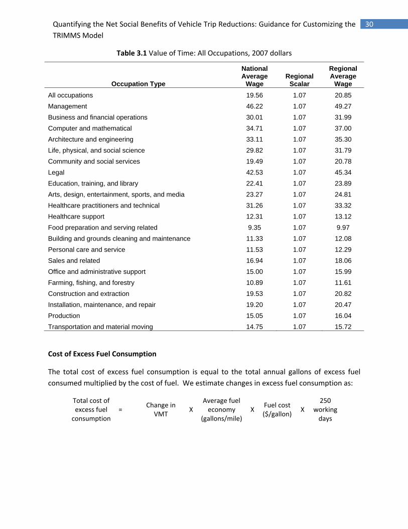
Following findings from a recently published NCTR report on the value of time [21], we measure the value of time for commuting purposes as 40 percent of the prevailing average wage rate. We use the current Bureau of Labor Statistics (BLS) average prevailing hourly wage rates by occupation type, scaled to account for cost of living differentials [22]. Following is an example of calculation of the average wage rate for the Tampa‐St. Petersburg‐Clearwater MSA.
Quantifying the Net Social Benefits of Vehicle Trip Reductions: Guidance for Customizing the TRIMMS Model
30
Table 3.1 Value of Time: All Occupations, 2007 dollars
Occupation Type
National Average
Wage Regional
Scalar
Regional Average
Wage All occupations 19.56 1.07 20.85 Management 46.22 1.07 49.27 Business and financial operations 30.01 1.07 31.99 Computer and mathematical 34.71 1.07 37.00 Architecture and engineering 33.11 1.07 35.30 Life, physical, and social science 29.82 1.07 31.79 Community and social services 19.49 1.07 20.78 Legal 42.53 1.07 45.34 Education, training, and library 22.41 1.07 23.89 Arts, design, entertainment, sports, and media 23.27 1.07 24.81 Healthcare practitioners and technical 31.26 1.07 33.32 Healthcare support 12.31 1.07 13.12 Food preparation and serving related 9.35 1.07 9.97 Building and grounds cleaning and maintenance 11.33 1.07 12.08 Personal care and service 11.53 1.07 12.29 Sales and related 16.94 1.07 18.06 Office and administrative support 15.00 1.07 15.99 Farming, fishing, and forestry 10.89 1.07 11.61 Construction and extraction 19.53 1.07 20.82 Installation, maintenance, and repair 19.20 1.07 20.47 Production 15.05 1.07 16.04 Transportation and material moving 14.75 1.07 15.72
Cost of Excess Fuel Consumption
The total cost of excess fuel consumption is equal to the total annual gallons of excess fuel consumed multiplied by the cost of fuel. We estimate changes in excess fuel consumption as:
Total cost of excess fuel consumption
= Change in
VMT X
Average fuel economy
(gallons/mile) X
Fuel cost ($/gallon)
X 250
working days

Quantifying the Net Social Benefits of Vehicle Trip Reductions: Guidance for Customizing the TRIMMS Model
31
We use TTI Urban Mobility Report equation A‐7 [20] to get the average fuel economy in congestion:
Average Fuel Economy in Congestion
= 8.8 + 0.25 X average peak period congested speed
For each area, we use the annual average cost per gallon of fuel net of taxes provided by the Energy Information Administration [19]. Taxes are a transfer from consumers to government or producers and do not represent an economic social cost.
Resources
Fuel Costs: Energy Information Administration Gasoline, Prices by Formulation, Grade, Sales Type http://tonto.eia.doe.gov/dnav/pet/pet_pri_allmg_d_nus_PTA_cpgal_m.htm
Average Hourly Wage Rates: Bureau of Labor Statistics: http://www.bls.gov/oes/oes_dl.htm
3.3.2 Health and Safety
Another relevant component of social costs is represented by health and safety costs. These include monetary costs, such as property and personal injury damages caused by collisions and cost avoidance activities, as well as nonmonetary costs, such as pain and loss of productivity.
Measurement
We estimate the comprehensive health and safety costs associated with vehicle crashes as the total social cost per accident by severity type multiplied by the number of crashes in each severity class; its product summed over all severity classes.
Accident Costs
We use the comprehensive cost estimates of from the National Highway Traffic Safety Administration (NHTSA) report on the economic impact of motor vehicle crashes [23]. The report provides estimate of average economic and comprehensive costs by maximum abbreviated injury scale (MAIS). Economic costs consist of loss of human capital, market productivity, household productivity, medical care, property damage, and travel delay. NHTSA does not recommend using economic costs for cost‐benefit ratios, since economic costs do not include the “willingness to pay” or intangible costs to avoid these events. The willingness to pay is included in the comprehensive cost estimates using a quality‐adjustment life years (QALYs) factor loss. The comprehensive cost estimates are presented in Appendix A of the same report (Blincoe et al., 2002, Table A‐1, pp. 62), which we report below in Table 3.2. We

Quantifying the Net Social Benefits of Vehicle Trip Reductions: Guidance for Customizing the TRIMMS Model
32
scale these costs for each region using the ratio of the region’s median household income to the U.S. median household income.
Table 3.2 Monetary and Nonmonetary Crash Costs ($/crash, 2002 dollars)
Property Damage Only
No Injury Minor Injury
Moderate Injury
Serious Injury
Severe Injury
Critical Injury
PDO MAIS 0 MAIS 1 MAIS 2 MAIS 3 MAIS 4 MAIS 5 Fatal
Medical ‐ 1
2,380
15,625
46,495
131,306
332,457
22,095
Emergency Services
31 22
97
212
368
830
852
833
Market Productivity
‐ ‐ 1,749
25,017
71,454
106,439
438,705
595,358
HH Productivity
47 33
572
7,322
21,075
28,009
149,308
191,541
Insurance Administration
116 80
741
6,909
18,893
32,335
68,197
37,120
Workplace Cost
51 34
252
1,953
4,266
4,698
8,191
8,702
Legal Costs ‐ ‐ 150
4,981
15,808
33,685
79,856
102,138
Subtotal 245 170
5,941
62,019
178,359
337,302
1,077,566
957,787
Non‐Injury Components
Travel Delay 803 773
777
846
940
999
9,148
9,148
Property Damage
1,484 1,019
3,844
3,954
6,799
9,833
9,446
10,273
Subtotal 2,287 1,792
4,621
4,800
7,739
10,832
18,594
19,421
QALYs ‐ ‐ 15,017
157,958
314,204
731,580
2,402,997
3,366,388
Total 2,532 1,962
10,562
66,819
186,098
348,134
1,096,160
977,208
Source: [23]1.
Change in Number of Crashes
To obtain the change in number of crashes, we multiply changes in VMT estimated by TRIMMS© by the crash rate of each severity.
1 The MAIS scale includes seven levels with: 0 = no injury; 1 = minor injury (whiplash, bruise); 2 = moderate injury (closed leg fracture, finger crush); 3 = serious injury (open leg fracture, amputated arm, major nerve laceration); 4 = severe injury (partial spinal cord severance, concussion); 5 = critical injury (complete spinal cord severance, concussion with loss of consciousness lasting more than 24 hours); Fatal (death).

Quantifying the Net Social Benefits of Vehicle Trip Reductions: Guidance for Customizing the TRIMMS Model
33
Crash Rates
Crash rates are positively related to traffic density, vehicle speeds, and roadway characteristics. For example, Kockelman [24] reports a nonlinear positive relationship between crash rates and vehicle speeds. Wand and Kockelman [25] find that crash rates vary according to vehicle type with light duty vehicles (minivans, pickups and sport utility vehicles) being associated with higher crash rates. Litman [26] provides empirical evidence that crashes increase with annual vehicle mileage and that mileage reduction reduces crashes and crash costs.
We use the National Highway Traffic Safety Administration Fatality Analysis Reporting System (FARS) to obtain estimate of crash rates in number of crashes per million VMT. These estimates are based on historical information on crashes for all vehicle types by KABCO severity, i, and by road functional classification, k:
, ,
where i = KABCO scale (K = killed; A = incapacitating injury; B = non‐incapacitating injury; C = possible injury; O = no injury); k = road functional classification (1 = arterial rural; 2 = arterial urban; 3 = freeway rural; 4 = freeway urban; 5 = collector rural; 6 = collector urban).
As an example, Table 3.2 reports crash rates for the State of Florida by injury and road functional classification. To substitute the default crash rates with area‐specific values the user can run a query on the FARS system (check the internet link below).
Table 3.3 Crash Rates (crashes/million VMT) ‐ Florida
Resources
Crash costs
The Economic Impact of Motor Vehicle Crashes, 2000: Appendix A, Table A‐1, pp.62. National Highway Traffic Safety Administration:
Injury Severity Interstate Arterial Collector Total Interstat Arterial Collector Total Total State
No Injury (0) 0.004 0.007 0.018 0.010 0.002 0.009 0.004 0.005 0.006
Possible Injury (C) 0.001 0.003 0.005 0.003 0.001 0.002 0.001 0.001 0.002Nonincapacitating Evident Injury (B) 0.003 0.005 0.009 0.006 0.001 0.003 0.001 0.002 0.003Incapacitating Injury (A) 0.004 0.006 0.012 0.008 0.001 0.003 0.001 0.002 0.003
Fatal Injury (K) 0.012 0.020 0.052 0.029 0.006 0.016 0.007 0.010 0.014
Total 0.024 0.042 0.097 0.055 0.011 0.033 0.014 0.021 0.027
Rural Urban

Quantifying the Net Social Benefits of Vehicle Trip Reductions: Guidance for Customizing the TRIMMS Model
34
http://www.nhtsa.dot.gov/staticfiles/DOT/NHTSA/Communication%20&%20Consumer%20Information/Articles/Associated%20Files/EconomicImpact2000.pdf
Crash rates by KABCO severity class
National Highway Traffic Safety Administration, Fatality Analysis Reporting System:
http://www‐fars.nhtsa.dot.gov/Main/index.aspx
Vehicle miles of travel by roadway type
Federal Highway Administration, Highway Statistics 2007, Highway Statistics Series:
http://www.fhwa.dot.gov/policyinformation/statistics/2007/vm2.cfm
3.3.4 Air Pollution
Air pollution costs refer to costs associated with motor vehicle use. Motor vehicles produce various harmful emissions that have negative effects at local and global levels. Exhaust air emission cause damage to human health, visibility, materials, agriculture and forests [4, 5]. The major source of pollutants include carbon monoxide (CO), volatile organic compounds (VOCs), nitrogen oxide (NOx), sulphur oxide (SOx), and particulate matter (PM). Mobile emissions also affect global climate as gases increase the global warming effect. We discuss this issue in the next section.
Measurement
Pollution costs are the product of three values:
• emission estimates, measured in grams/mile;
• emission costs, measured in $/gram
• vehicle miles of travel (VMT), estimated by TRIMMS.
For each mode i and each pollutant k, the total pollution cost PC is equal to:
∑ $
These values are summed across all vehicle classes, pollutants, and impact categories to produce estimates of total pollution benefits of each TDM strategy being evaluated.
Emission Estimates
To obtain accurate emission estimates we used the Environmental Protection Agency’s (EPA) latest vehicle emission factor model MOBILE6.2 [27]. We run the model for each metropolitan statistical area, distinguishing between freeway and arterial travel conditions, and accounting

Quantifying the Net Social Benefits of Vehicle Trip Reductions: Guidance for Customizing the TRIMMS Model
35
for summer and winter temperatures for a total of 340 runs. The set up of MOBILE6.2 input files is based on the following assumptions:
• Average passenger vehicle age of 8 years
• Average transit vehicle age of 7 years
• Freeway and arterial estimated average speeds
• Average ambient temperature, winter and summer time
• Standard operating mode (cold‐start, hot‐start, stabilized), no inspection/maintenance or anti‐tampering programs, and gasoline volatility of 8.7 per square inch RBP (Reid vapor pressure).
The U.S. National Transportation Statistics (Table 1‐25 and Table 1‐28a) reports average passenger and transit vehicle age. The Texas Transportation Institute Urban Mobility Report provides average freeway and arterial speeds by major metropolitan statistical area [20]. Historical summer and winter average ambient temperatures for each of the metropolitan statistical are available online from the website weather.com. All other assumptions represent Mobile 6 default input values.
Pollution Emission Costs
Pollution emission costs are measured in $/Kg damages related to health and visibility impacts and physical impacts on the environment. We adopted the costs estimates of Delucchi [4], who estimated costs for several impact categories for urban areas of the U.S. in 1991. Delucchi recently updated the original values to account for changes in information about pollution and its effects [10]. He customizes these estimates by using regional exposure scalars to get from the average exposure basis in U.S. urban areas to the average exposure in each of the metropolitan statistical areas. According to Delucchi, population density is the best simple measure of exposure to air pollution. This exposure scalar is equal to the ratio of population density in each individual area to the average urban‐area population density in the original analysis of 1991 (2,150 persons per square mile).
The original 1991 $/Kg are scaled to 2009 dollar values using the consumer price index (CPI). To account for cost of living geographical differences, these estimates are scaled to each individual region using the ratio of median household income of each area to the U.S. median household income.
Table 3.4 provides an example of regionalization of pollution costs for the Tampa‐Saint Petersburg‐Clearwater metropolitan statistical area. It shows the calculation of health costs related to NOx emissions.

Quantifying the Net Social Benefits of Vehicle Trip Reductions: Guidance for Customizing the TRIMMS Model
36
Table 3.4 Example of Parameter Regionalization ‐ NOX Health Emissions
Resources
Average Age of Passenger Vehicles
Bureau of Transportation Statistics, National Transportation Statistics, Table 1‐25: Average Age of Automobiles and Trucks in Operation in the United States (Years)
http://www.bts.gov/publications/national_transportation_statistics/html/table_01_25.html
Average Age of Urban Transit Vehicles
Bureau of Transportation Statistics, National Transportation Statistics, Table 1‐28a: Average Age of Urban Transit Vehicles (Years)
http://www.bts.gov/publications/national_transportation_statistics/html/table_01_28a.html
National Emission Levels
Table 4‐38: Estimated National Average Vehicle Emissions Rates per Vehicle by Vehicle Type using Gasoline and Diesel
http://www.bts.gov/publications/national_transportation_statistics/html/table_04_38.html
Mobile 6 Vehicle Emission Modeling Software
Software is available for download at the EPA website: http://www.epa.gov/otaq/m6.htm
Cost Type 1991 $/kg
2009 CPI/1991
CPI
Population Density
(persons/mile2)
U.S. Population Density
(persons/mile2)
exposure Scalar (C/D)
Regional Cost of Living Index 2008 $/Kg
(A) (B) ( C ) (D) (E) (F) (A* B * E *F)
Health 187.50 1.52 938 2150 0.44 0.96 119.05

Quantifying the Net Social Benefits of Vehicle Trip Reductions: Guidance for Customizing the TRIMMS Model
37
3.3.5 Global Climate Change
The Intergovernmental Panel on Climate Change (IPCC) defines climate change as the “state of any change in climate over time, whether due to natural variability or as a result of human activity [6].” Trapped heat in the atmosphere is a major driver of global climate change. Gases that trap heat in the atmosphere are called greenhouse gases. These include carbon dioxide (CO2), methane CH4, nitrous oxide N2O and fluorinated gases [7]. Motor vehicle fuel production and consumption release greenhouse gases, mainly CO2, a major contributor to global climate change. EPA estimates that CO2 represents about 30 percent of all greenhouse gas emissions. There are mitigation and damage costs associated with global climate change. Damage costs are costs related to the environment, health, and reduced economic productivity.
Measurement
We estimate the global climate change costs (GCCC) for each mode i as:
∆ $
where ∆ is the change in VMT for mode i estimated by TRIMMS; represent
CO2 emissions estimated by MOBILE6; and $ is the marginal damage cost associated with
CO2 emissions.
Marginal Damage Costs of CO2 Emissions
We estimate the marginal damage costs, or the cost of a change in greenhouse gas emissions associated with motor vehicle use. The unit of measure is the marginal damage in US dollars caused by a metric ton of CO2 emissions ($/tC). Since cost estimates vary widely across the literature, we adopt the estimate of $50/tC by Tol [28] who reviewed who analyzed and combined 103 estimates of marginal damage costs of carbon dioxide emissions from 28 published studies. We use the mean marginal damage cost that takes into account of only peer‐reviewed literature (pp.2070). We multiply this estimate by 10‐6 to scale it down to dollar per gram ($/g), since MOBILE6 estimates CO2 emissions in g/mile.
Note that while we only consider the marginal damage costs associated with CO2 emissions, other authors provide more comprehensive estimates of greenhouse emission costs. For example, Delucchi [10] considers the global emission costs of pollutants other than CO2 by calculating a ratio of CO2 equivalent emissions to CO2 emissions. Since EPA [7, 8, 29] considers these other greenhouse gases as more volatile and difficult to estimate, we follow EPA approach that only models CO2 global emissions.

Quantifying the Net Social Benefits of Vehicle Trip Reductions: Guidance for Customizing the TRIMMS Model
38
3.3.6 Noise Pollution
Noise costs refer to negative externalities associated with motor vehicle noise emissions. Motor vehicles produce noise from engine acceleration and vibration, from tire contact on road surfaces, from break and horn usage. Noise disrupts sleep, activities, causes stress, and negatively affects property values.
Measurement
We measure the total cost of noise emissions (NC) as:
∆ $
where ∆ is the change in VMT for mode i estimated by TRIMMS; represents noise with k indicating rural or urban area.
Noise costs
Several studies monetize traffic noise costs (see for example, Delucchi [30]. We use noise cost estimates by Tod Litman [31], who comprehensively reviews the literature and provides estimates by mode type for urban and rural areas. These estimates are reproduced in the table below. In TRIMMS© these costs are scaled to account for cost of living differentials between national averages and each regional area.
Table 3.5 Noise Pollution Costs
Mode Urban Peak
Urban Off‐Peak Rural Average
Average Car 0.013 0.013 0.007 0.011 Van/Light Truck 0.013 0.013 0.007 0.011 Rideshare Passenger 0.000 0.000 0.000 0.000 Diesel Bus 0.066 0.066 0.033 0.053 Motorcycle 0.132 0.132 0.066 0.106 Bicycle 0.000 0.000 0.000 0.000 Walk 0.000 0.000 0.000 0.000 Telecommute 0.000 0.000 0.000 0.000
Source: [31]

Quantifying the Net Social Benefits of Vehicle Trip Reductions: Guidance for Customizing the TRIMMS Model
39
3.4 Guidance on How to Update Input Parameters
3.4.1 Global and Regional Inputs
The user can change all global and regional input parameters. This is accomplished by clicking on the Model Parameters button located in the Results sheet. This activates the module shown in Figure 3.1. This module consists of three steps that allow changing global, regional, and cost parameters for all social costs. In the first step, the user can modify all global parameters. In step two, shown in Figure 2.2, the user can modify all regional parameters.
Figure 3.1 Model Parameters Module: Global Parameters

Quantifying the Net Social Benefits of Vehicle Trip Reductions: Guidance for Customizing the TRIMMS Model
40
Figure 3.2 Model Parameters Module: Regional Parameters
3.4.2 Social Cost Parameters
In the third step (Step 3) of the Model Parameters module, the user can change all of the default parameters associated with the social costs. Step 3 consists of five tabs that allow modifying each of the social costs. We refer the user to the previous sections of this chapter for the sources to retrieve inputs to customize these parameters.
Upon clicking on the Finish button, TRIMMS© accepts all changes the user has made. Next, the user must re‐run the analysis to use the customized parameters. Clicking on the Run Analysis button will recall the analysis back will all information previously filled. Clicking the Model Reset button allows returning to the default parameters.

Quantifying the Net Social Benefits of Vehicle Trip Reductions: Guidance for Customizing the TRIMMS Model
41
Figure 3.3 Model Parameters Module: Air Pollution Costs
Figure 3.4 Model Parameters Module: Congestion Costs

Quantifying the Net Social Benefits of Vehicle Trip Reductions: Guidance for Customizing the TRIMMS Model
42
Figure 3.5 Model Parameters Module: Global Climate Change Costs
Figure 3.6 Model Parameters Module: Health and Safety Costs

Quantifying the Net Social Benefits of Vehicle Trip Reductions: Guidance for Customizing the TRIMMS Model
43
Figure 3.7 Model Parameters Module: Noise Pollution Costs
3.5 Trip Demand Functions Elasticity Parameters
As explained in more detail in Appendix A, TRIMMS© estimates changes in trips using trip demand functions that rely on certain parameter estimates to properly function. These parameters are defined as elasticities and they measures users’ responsiveness to changes in pricing and travel times. Economists define the term elasticity as the percentage change in demand of a good caused by a one‐percent change in its price or other characteristics. For example, an elasticity of ‐0.5 for single occupancy vehicle trips with respect to fuel costs means that each 1 percent increase in the price of fuel results in a 0.5 percent reduction in the demand for vehicle trips.
TRIMMS© trip demand functions make use of direct elasticities and cross elasticities. Direct elasticities refer to the percentage change in the demand for trips of any given mode resulting from a change in its own price or other measurable characteristics. Cross elasticities refer to the percentage change in the demand for trips of any given mode caused by a change in price or other measurable characteristics of other modes. For example, an increase in parking prices causes a direct negative percent change in the demand for auto trips and causes a positive change in the demand for transit services. The use of cross elasticities recognizes a certain degree of substitution, or mode shift, between transport modes; the intensity of substitution depending on circumstances and measured by the cross elasticities.

Quantifying the Net Social Benefits of Vehicle Trip Reductions: Guidance for Customizing the TRIMMS Model
44
To obtain default parameters, we surveyed the empirical literature. There are a number of excellent surveys of the empirical literature on the demand for transportation and the role of elasticities [32‐35]. TRIMMS© uses parameters from these studies and other publications. For example the estimated
Fare (and in general, pricing) elasticities are dynamic, as they vary over time. Researchers distinguish between short run and long run elasticity estimates. There are many definitions of short and long run, but most author define short run to be 1 or 2 years, and the long run to be about 12 to 15 years. Since most of the TDM programs run for a period corresponding to the short run, we adopted short run estimates as default values. These estimates are on average lower than the long run, signifying that users are less responsive to price changes in the immediate. The user can change all elasticity parameters, by clicking on the Modify Elasticities button located in the Results sheet. Table 3.6 reports the default values estimates for direct and cross fare and price elasticities.
Table 3.6 Fare and Price Elasticities
Mode Elasticity Source Notes
short run long run
Auto ‐ Drive Alone
Direct ‐0.11 Litman (VTPI) Table 22, pp.27
Cross‐Price: Transit 0.03 0.15 Litman (VTPI) We use the lower ranges
Auto ‐ Rideshare
Direct
Cross‐Price: Transit 0.03 0.15 Litman (VTPI) same as auto‐drive alone
Vanpool
Direct ‐0.73 ‐1.46 Concas et al. Long run twice of short run
Cross‐Price: Auto ‐ Rideshare n/a n/a n/a n/a
Transit Direct: Peak ‐0.05 ‐0.33 Graham et al.
Direct: Off‐Peak ‐0.10 ‐0.66 Our assumptionOur assumption: assume twice of peak
Cross‐Price: Auto ‐ Drive Alone 0.05 0.20 Litman (VTPI) We use the lower ranges
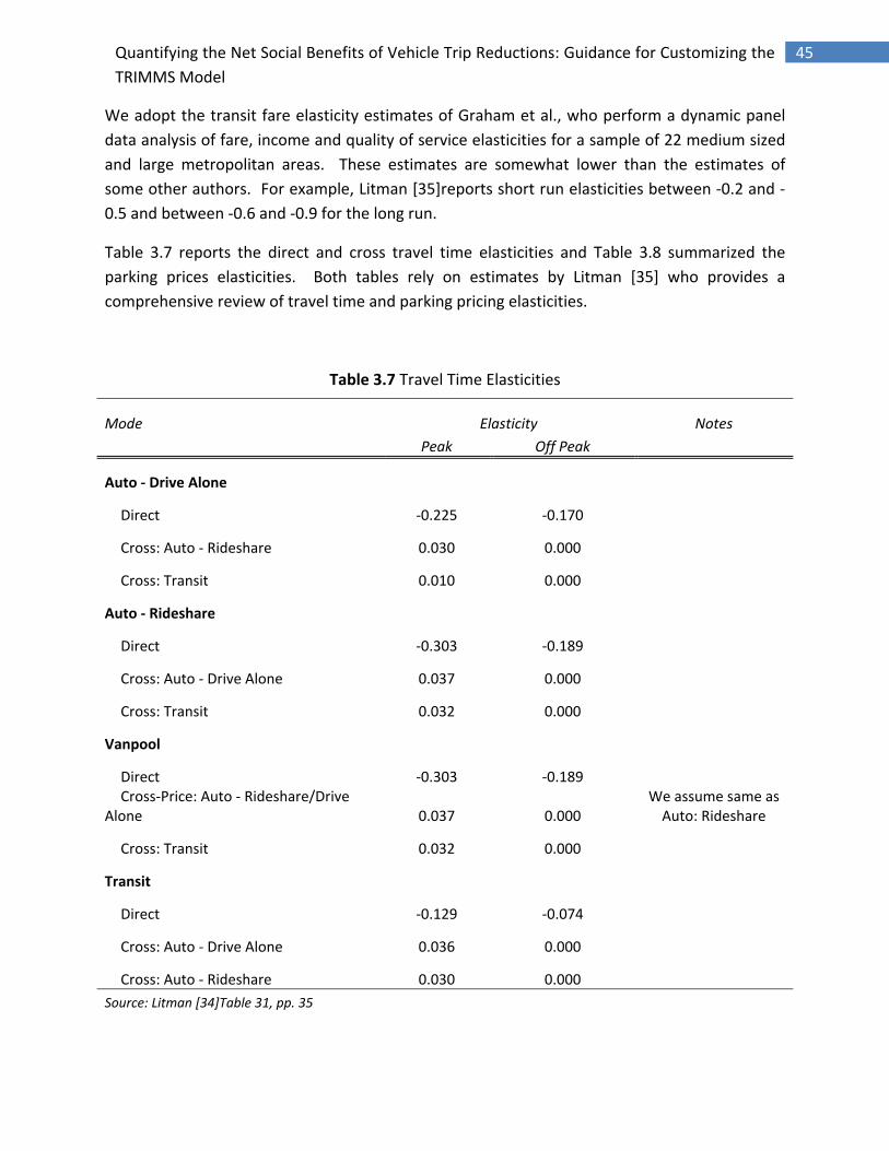
Quantifying the Net Social Benefits of Vehicle Trip Reductions: Guidance for Customizing the TRIMMS Model
45
We adopt the transit fare elasticity estimates of Graham et al., who perform a dynamic panel data analysis of fare, income and quality of service elasticities for a sample of 22 medium sized and large metropolitan areas. These estimates are somewhat lower than the estimates of some other authors. For example, Litman [35]reports short run elasticities between ‐0.2 and ‐0.5 and between ‐0.6 and ‐0.9 for the long run.
Table 3.7 reports the direct and cross travel time elasticities and Table 3.8 summarized the parking prices elasticities. Both tables rely on estimates by Litman [35] who provides a comprehensive review of travel time and parking pricing elasticities.
Table 3.7 Travel Time Elasticities
Mode Elasticity Notes
Peak Off Peak
Auto ‐ Drive Alone
Direct ‐0.225 ‐0.170
Cross: Auto ‐ Rideshare 0.030 0.000
Cross: Transit 0.010 0.000
Auto ‐ Rideshare
Direct ‐0.303 ‐0.189
Cross: Auto ‐ Drive Alone 0.037 0.000
Cross: Transit 0.032 0.000
Vanpool
Direct ‐0.303 ‐0.189We assume same as Auto: Rideshare
Cross‐Price: Auto ‐ Rideshare/Drive Alone 0.037 0.000
Cross: Transit 0.032 0.000
Transit
Direct ‐0.129 ‐0.074
Cross: Auto ‐ Drive Alone 0.036 0.000
Cross: Auto ‐ Rideshare 0.030 0.000 Source: Litman [34]Table 31, pp. 35

Quantifying the Net Social Benefits of Vehicle Trip Reductions: Guidance for Customizing the TRIMMS Model
46
Table 3.8 Parking Pricing Elasticities
Parking Elasticities
Trip Purpose Auto ‐ Drive Alone Auto ‐ Rideshare Transit Slow Modes
Commuting ‐0.08 0.02 0.02 0.02 Source: Litman (2008), Table 13, pp. 17
3.5.1 Guidance on How to Update Elasticity Parameters
The user can change all elasticity parameters by clicking on the Modify Elasticities. This action shows a hidden worksheet called Elasticities. In this sheet, the user can enter custom values, which override the default ones. The user manual included in with the model shows step‐by‐step instructions on how to enter these values.
Figure 3.8 Elasticities Worksheet

Quantifying the Net Social Benefits of Vehicle Trip Reductions: Guidance for Customizing the TRIMMS Model
47
Chapter 4: Sensitivity Analysis Module
4.1 Introduction
As discussed in Chapter 2, the Results sheet provides a summary of travel impacts and change in social costs. As useful and informative as these results are for project evaluation, they represent a single point estimate and are defined as deterministic in statistical terms. They must be taken as true estimates with no possibility of random variation. In fact, if we were to run the model multiple times, we would get the same results repeatedly. As seen in Chapter 3, this is not exactly what happens in reality as the evaluation of social costs is characterized by uncertainty and variability. With single point estimates there is no way to corroborate the validity of results. Some sketch planning tools provide two scenarios using high and low ranges of point estimates. Usually the analyst must conduct a sensitivity analysis of factors most likely to affect the analysis. A less subjective but technically challenging way to validate results is to conduct a sensitivity analysis using Monte Carlo (MC) simulation methods. This chapter discusses TRIMMS© sensitivity analysis module in detail. We define MC simulation and explain how TRIMMS© uses this method to corroborate the estimation results and to provide additional program cost effectiveness benchmarking measures. Finally, we show step by step how to conduct this analysis using an application example.
4.2 Monte Carlo Simulation
The definition of Monte Carlo was created by some physicists during the World War II Manhattan Project because of the similarity of the method to capital of Monaco’s famous games of chance [36]. These methods are useful for modeling events with significant uncertainty in the values of inputs. MC simulation is now used routinely to study a broad array of physical phenomena involving randomness. This is especially true in the case of TDM evaluation, where there is a lot of uncertainty regarding the potential impact of TDM in terms of mode share changes and the resulting benefits.
MC simulation deals with uncertainty by treating the model’s input parameters as variables subject to random variation. Because MC simulation is based on repeated sampling from a random process, it must rely on a process to simulate this random variation. This process is offered by computer programs like Excel, which have built‐in random number generators. In TRIMMS, we use an improvement to the Excel random generator to develop a statistical dataset that accounts for random variation in the input parameters. The algorithm is run many times to provide simulated ranges for the input parameters and assess which factors might be responsible for variability and uncertainty in the model outcome.

Quantifying the Net Social Benefits of Vehicle Trip Reductions: Guidance for Customizing the TRIMMS Model
48
To set up the MC simulation we must follow these steps:
1‐ Assume what inputs to treat as random variables 2‐ Assume which family of probability distributions these belong to 3‐ Decide how many times to run the simulation
In TRIMMS, we assume that all social costs are random variables coming from log‐normal distributions that are truncated at their minimum and maximum values. For example, the costs associated with each pollutant take the minimum and maximum values as in Delucchi [17], but we assume that in each MC simulation run these costs can take any positive value between the minimum and the maximum. We treat all other social costs, with the exception of gasoline cost, in the same manner. We treat gasoline cost as a random variable from a log‐normal distribution with a mean value equal to the mean fuel cost. The mean and standard deviation come from the Energy Outlook Report by the Energy Information Administration, which provides medium and long‐term fuel cost forecasts, including standard deviation estimates.
We treat accident rates as random variables generated by a truncated log‐normal distribution. The minimum and maximum values that this distribution can take correspond to the accident rates of freeway and arterial conditions, while its mean is assumed to correspond to the accident rate for all roadway types.
Finally, we set the number of runs in each simulation at 10,000 iterations. We then run a simulation using peak values and another run for off‐peak values. The relatively high number of iterations ensures that the estimation of the probability distribution approximates to the true underlying parameters. To run the MC simulation, we implemented a Visual Basic macro that uses the Barreto/Howland [36] random number generator. This random number generator improves upon the default Excel random number generator in terms of better approximation to true randomness. Figure 4.1 shows the result of the MC simulation of excess fuel consumption costs.

Quantifying the Net Social Benefits of Vehicle Trip Reductions: Guidance for Customizing the TRIMMS Model
49
Figure 4.1 Monte Carlo Simulation Example: Changes in Fuel Consumption Costs
This figure displays the simulated mean, minimum and maximum values. Minimum and maximum values are equal to the 5th and 95th percentiles of the above distribution. Note that the initial estimate of $‐7.62/day from the Results sheet (displayed in Figure 4.2) is close, but not equal, to the mean of $‐8.7/day of Figure 4.1. After the MC simulation, the estimate of changes in excess fuel consumption costs is not longer one point estimate but a range of estimates. Analysts and decision makers can answer additional questions using MC simulation. For example, one might be interested in knowing the probability that the estimated fuel cost reductions are actually equal to TRIMMS© single point estimate or equal to a predetermined quantity. This question becomes more relevant when simulating ranges in B/C ratio, which is at the core of TRIMMS© simulation module.
4.3 Running TRIMMS© Sensitivity Analysis Module
As shown in Chapter 2, the Results sheet provides a summary of travel impacts and estimates of program benefits and costs. Figure 4.2 provides a close‐up of these estimates. TRIMMS© estimates changes in trips, VMT, and mode shares with respect to the baseline information entered. TRIMMS© then estimates the changes in six major categories of social costs. A reduction in social costs represents a benefit attributable to the TDM program under evaluation. The sum of these daily benefits over the number of working days in a year gives the
0
100
200
300
400
500
600
700
800
900
1000
-$21.74 -$19.33 -$16.92 -$14.51 -$12.10 -$9.69 -$7.28 -$4.87
Change in Excess Fuel Consumption Costs ($/Day)
‐8.7Mean
Min
Max
‐13.1
‐5.4

Quantifying the Net Social Benefits of Vehicle Trip Reductions: Guidance for Customizing the TRIMMS Model
50
Total Annual Benefits. To obtain the Total Annualized Cost, the program total cost is annualized using the following formula described in Chapter 3.
The ratio of Total Annual Benefits to the Total Annualized Cost produces the Benefit to Cost Ratio:
This measure provides an economic assessment of how cost‐efficient a TDM program is while producing positive benefits. The benefit to cost (B/C) ratio can be used as a cost effectiveness benchmark. A ratio equal to 1.0 indicates that for each dollar spent on the TDM program under evaluation there is a one‐dollar return in terms of social benefits. Usually, the prioritization of transportation infrastructure investments for funding appropriation relies on the B/C ratio to produce a project‐ranking list.
Figure 4.2 Summary of TDM Costs and Benefits taken from Results Sheet
In TRIMMS, the MC simulation module is set up to treat all benefits as random variables. We treat the total annualized cost as deterministic (not subject to variation). One could consider this cost as a random variable, but this issue is beyond the scope of this study and a potential future enhancement. Given the above formula, the resulting B/C ratio is itself a random variable. We are interested in estimating its mean and the minimum and maximum values defining the 5th and 95th lower and upper boundary values of its distribution. These values give us an idea of how likely the single point estimates of Figure 4.2 are to occur if we were to implement the TDM strategy under evaluation over and over again. Another question that the simulation can help answer is: “What is the probability that the B/C ratio will at least be greater than a certain value?” Often, transportation analysts are interested in knowing if the B/C cost

Quantifying the Net Social Benefits of Vehicle Trip Reductions: Guidance for Customizing the TRIMMS Model
51
ratio will at least greater than 1.0 to guarantee some returns over each dollar invested in the program.
Suppose the user runs an analysis and obtains the results of Figure 4.2. The B/C ratio is equal to 1.09 and to 0.94 for the peak and off‐peak period respectively. The user wants to test: 1) how likely are these numbers to vary due to input cost parameter variation, and 2) what is the probability that these values will be greater than 1.0 or any other threshold value.
To answer this question the user must activate the simulation module. This is done by clicking on the Sensitivity Analysis button located on the Results sheet (note that to run this module the user must first conduct the analysis as described in Chapter 2), which launches the screen shown in Figure 4.3.
Figure 4.3 Sensitivity Analysis Prompt Screen
By default, TRIMMS© runs 10,000 iterations. On a typical personal computer (3.0 gigahertz processor and 2.0 gigabytes of random access memory) the simulation takes about one minute. To run the simulation faster, the user can reduce the number of iterations. We strongly suggest not going under 3,000 iterations to guarantee statistical robustness of the results.
On this screen, the user can set up a target B/C ratio to estimate that probability that the B/C ratios estimated by TRIMMS© and reported in the Result sheet will be greater than that value. In this example, we set a target B/C ratio equal to one. If the user leaves this cell empty, then

Quantifying the Net Social Benefits of Vehicle Trip Reductions: Guidance for Customizing the TRIMMS Model
52
the default B/C targets are the B/C ratios for peak and off‐peak periods reported in the Result sheet. Upon clicking on the Ok button, the MC simulation starts. A progress status bar located on the bottom left side of TRIMMS© shows percent completion information.
Figure 4.4 MC Simulation Progress Status Bar
Once the simulation is completed the Sensitivity sheet appears and show the results of MC simulation, as shown in Figure 4.5.
Figure 4.5 TRIMMS© Sensitivity Analysis Results
The charts of Figure 4.5 display the simulated B/C ratio distributions, the distribution mean and the minimum (5th percentile) and maximum (95th percentile) values. The table under the charts reports the original single point estimates for the Results sheet. On the top right hand of each chart is the estimated probability that the B/C ratio is greater than the target value. For this example, the probability that the B/C ratio is greater than 1.0 is equal to 100 percent and 99.4 percent for the peak and off‐peak periods. Looking at the distributions this result is to be expected as the simulated mean B/C ratio is 1.6 and 1.4 for peak and off‐peak period respectively.
Next, we wish to know the probability that the B/C ratio will be greater than two. We are interested in knowing the likelihood that the TDM program being evaluated will return at least $2 for each $1 invested in it. To do so, we click on Back to Results button and we re‐run the

Quantifying the Net Social Benefits of Vehicle Trip Reductions: Guidance for Customizing the TRIMMS Model
53
simulation setting up a B/C target ratio to 2.0 as shown in Figure 4.5. To expedite the simulation, we set the iterations at 5,000 runs.
Figure 4.6 Sensitivity Analysis with B/C target set at 2.0
Figure 4.6 displays the results. The probability that the B/C ratio is greater than two is equal to 2.7 and 0.0 percent for the peak and off‐peak periods respectively. Assuming that the agency had a B/C threshold of 2.0 for project selection purposes, it would have rejected this TDM strategy.

Quantifying the Net Social Benefits of Vehicle Trip Reductions: Guidance for Customizing the TRIMMS Model
54
Figure 4.7 Sensitivity Analysis Results with B/C target set at 2.0

Quantifying the Net Social Benefits of Vehicle Trip Reductions: Guidance for Customizing the TRIMMS Model
55
Chapter 5: Conclusions This research project reports the results of a series of enhancement to the Trip Reduction Impacts of Mobility Management Strategies (TRIMMS©) model. The model new version (or Version 2.0) includes a series of improvements that allow TDM practitioners better customization of input parameters and disaggregation of TDM benefits. TRIMMS© now includes default input parameters for 85 metropolitan statistical areas, which cover several small, large, medium and very large urban areas across the U.S.
One of the project tasks was updating the TRIMMS© model to allow more customization, and to clearly differentiate between analysis at the regional and employer‐site levels. Furthermore, the module that evaluates the impact of employer support programs is revised. This includes a refinement of the employer support program evaluation module, which employs parameters estimated by a panel data regression analysis of commuter trip reduction programs.
Recognizing that there is uncertainty in the value of inputs such as cost of accidents, emissions costs, we added an extended capability to allow for Monte Carlo simulation of the impact estimates. Monte Carlo simulation uses random sampling from probability distribution functions as model inputs to produce a sensitivity analysis. As part of this update, we developed a specific algorithm that generates random variation in the input parameters. This effort resulted in the design of a module that permits sensitivity analysis, a feature to date not present in any other spreadsheet application of this kind. The simulation can help practitioners estimate the probability that the B/C ratio will at least be greater than some predetermined benchmarking value. This feature allows conducting TDM evaluation to meet the Federal Highway Administration Congestion and Air Quality (CMAQ) Improvement Program requirements for program effectiveness assessment and benchmarking. [1].
5.1 Model Limitations
As any other sketch‐planning tool, TRIMMS has limitations that come from the need to aggregate data and the assumptions related to trip and mode share change estimation. Some of these limitations are the result of a trade‐off between the need to strike a balance between the complexity and intensive data needs of traditional transportation analysis tools (like regional travel forecasting models) and the substantial time and cost savings of sketch‐planning applications. TRIMMS simplifies the quantification requirements for TDM programs by making careful simplifications, as well as enhancements.

Quantifying the Net Social Benefits of Vehicle Trip Reductions: Guidance for Customizing the TRIMMS Model
56
In addition, some of TRIMMS limitations are due to data‐gathering related to the estimation of TDM benefits and to the use of elasticities to measure travelers’ responsiveness to price and travel time changes.
We considered a subset of all relevant benefits that TDM strategies can produce by focusing on those that can be explicitly and more easily measured. The literature shows that TDM provides benefits that go beyond emission reductions, health and safety, global climate change, excess fuel consumption, noise pollution [2]. TDM benefits extend to land‐use through the more efficient pricing and allocation of land and improvements in accessibility. TDM can also affect economic productivity. For example, the provision of flexible working schedule and telecommuting arrangements might results in increased employee productivity. TDM can also have positive health impacts in terms of improved fitness by promoting non‐motorized travel. Our choice of a subset of these benefits relies on the necessity to conduct program effectiveness and benefit‐to‐cost evaluation which require monetization of benefits. Not all of the above benefits can be quantified and therefore cannot be used for benefit‐to‐cost ratio computation.
Although there is a vast literature on the estimation of price and travel time elasticities, which are at the core of the model’s trip demand functions, analysts must put care in deciding which parameters to use for transportation planning and evaluation purposes. The elasticities we report in Chapter 3 are the results of various studies each subject to many factors that affect how users react to price and travel time changes. By developing the sensitivity analysis module, we account for the variability in estimates by introducing Monte Carlo simulation into the evaluation process to corroborate the estimation results.
Another limitation we must note is related to the estimation of global climate change impacts. We only consider the marginal damage costs associated with CO2 emissions, while other authors provide more comprehensive estimates of greenhouse emission costs. For example, Delucchi [10] considers the global emission costs of pollutants other than CO2 by calculating a ratio of CO2 equivalent emissions to CO2 emissions. Since EPA considers these other greenhouse gases as more volatile and difficult to estimate we followed EPA approach that only models CO2 global emissions. As the new EPA model will be made available, we intend to integrate CO2 emissions with other greenhouse gases responsible for global climate change.
5.2 Directions for Further Research
TRIMMS© 2.0 provides significant improvements over the earlier version. Still, there are areas where the tool could be expanded. For example, one future enhancement to TRIMMS© 2.0 could provide guidance on estimating the costs for the various TDM programs rather than treating total program costs as a single input.

Quantifying the Net Social Benefits of Vehicle Trip Reductions: Guidance for Customizing the TRIMMS Model
57
• While TRIMMS© 2.0 focuses on the social benefits of TDM, the effectiveness of TDM programs depends on employer cooperation and policies supporting these strategies.
• Employees’ use of transit depends on the compatibility of the work hour policies, such as flextime. The effectiveness of advanced traveler information systems to alter arrival and departure times to avoid congested periods depends on those same employer policies.
• Employer work‐life friendly programs such as compressed workweek programs and telework influence when or if a commute trip is made.
• Employer parking policies determine the availability and price of parking that influence mode choice by employees.
• Employer provision of bike and locker facilities can make the difference between someone choosing to drive or use a non‐motorized method.
TDM provides a variety of benefits to employers as well as society. Telework programs can improve productivity, enhance recruitment and retention of employees, and reduce absenteeism. Compressed work week programs enable the employer to expand coverage to enhance customer service. Employers allowing employees to pay for transit passes and parking as a pre‐tax benefit save payroll taxes. While most of the tools available to assess the impacts of TDM strategies focus on air quality benefits, there is a lack of tools to assist employers in assessing the costs and potential business benefits of implementing TDM programs [37]. One direction for further research is to extend TRIMMS capabilities to extend TDM evaluation to quantify the direct benefits to employers. These key benefits, such changes in employee productivity and reduction in turnovers, have significant impacts on the costs of doing business. A possible extension would be to develop a separate version of the model that estimates and summarizes this type of benefits. A return‐on‐investment approach based on these employer benefits and costs, augmented by the Monte Carlo analysis, could be perceived as a very useful tool to commuter assistance programs that work with employers in establishing TDM programs at worksites.
Finally, integrating TRIMMS© 2.0 as an off‐model to be used with the four‐step regional transportation planning models could assist transportation planners in estimating the impacts on traffic flows and traffic congestion in particular corridors due to TDM. TRIMMS© 2.0 could modify the mode choice and trip generation inputs to the regional models for that purpose.

Quantifying the Net Social Benefits of Vehicle Trip Reductions: Guidance for Customizing the TRIMMS Model
58
References 1. FHWA, Publication of Final Guidance on the Congestion Mitigation and Air Quality
Improvement (CMAQ) Program, F.H. Administration, Editor. 2008. 2. Litman, T., Energy Conservation and Emission Reduction Strategies, in TDM
Encyclopedia, V.T.P. Institute, Editor. 2008, Victoria Transport Policy Institute: Victoria. 3. Concas, S. and P.L. Winters, Economics of Transportation Demand Management (TDM),
N.C.f.T. Research, Editor. 2007, Center for Urban Transportation Research: Tampa. 4. Delucchi, M., Summary of the Nonmonetary Externalities of Motor‐Vehicle Use, in The
annualized social cost of motor‐vehicle use in the United States, based on 1990‐1991 Data. 1998, Institute of Transportation Studies.
5. Litman, T., Air Pollution Costs, in Transportation Cost and Benefit Analysis ‐ Techniques, Estimates and Implications, V.T.P. Institute, Editor. 2009, Victoria Transport Policy Institute: Victoria.
6. Bernstein, L., et al., Climate Change 2007: Synthesis Report, in An Assessment of the Intergovernmental Panel on Climate Change. 2007, Intergovernmental Panel on Climate Change.
7. EPA. Greenhouse Gas Emission. Climate Change 2009 [cited 2009 January, 2009]; Available from: http://www.epa.gov/climatechange/emissions/index.html.
8. EPA, Greenhouse Gas Emissions for the U.S. Transportation Sector 1990‐2003, U.S.E.P.A.O.o.T.a.A. Quality, Editor. 2006, U.S. Environmental Protection Agency: Fairfax.
9. Kuzmyak, J.R., et al., Procedures Manual for the COMMUTER Model v2.0, O.o.T.a.A. Quality, Editor. 2005, U.S. Environmental Protection Agency
10. Delucchi, M., The Social‐Cost Calculator (SCC): Documentation of Methods and Data, and Case Study of Sacramento. 2005, Institute of Transportation Studies.
11. ACS, American Community Survey (ACS). 2007, U.S. Census Bureau. 12. OMB, Guidelines and Discount Rates for Benefit‐Cost Analysis of Federal Programs,
O.o.M.a. Budget, Editor. 2009, Office of Management and Budget: Washington, DC`. 13. BLS, Consumer Price Index ‐ All Urban Consumers. 2009, Bureau of Labor Statistics. 14. NHTS, National Household Travel Survey. 2001. 15. Sinha, K.C. and S. Labi, Impacts on Energy Use. Transportatio decision making: principles
of project evaluation and programming. 2007: John Wiley & Sons. 16. FHWA, HERS‐ST Technical Report, in HERS ‐ST Highway Economic Requirements System‐
State Version, F.H. Administration, Editor. 2000. 17. Delucchi, M., The Annualized Social Cost of Motor‐Vehicle Use in the U. S., 1990‐1991:
Summary of Theory, Data, Methods, and Results, in The annualized social cost of motor‐vehicle use in the United States, based on 1990‐1991 Data. 1996, Institute of Transportation Studies.
18. Census, U.S., U.S. Census Summary File 3 (SF3). 2000. 19. EIA, Gasoline Prices by Formulation, Grade, Sales Type. 2009, Energy Information
Administration. 20. Schrank, D. and T. Lomax, The 2007 Urban Mobility Report, T.T. Institute, Editor. 2007,
Texas Transportation Institute: College Station.

Quantifying the Net Social Benefits of Vehicle Trip Reductions: Guidance for Customizing the TRIMMS Model
59
21. Concas, S. and A. Kolpakov, Synthesis of Researh on the Value of Time and Value of Reliability of Travel Time, N.C.f.T. Research, Editor. 2009, Center for Urban Transportation Research: Tampa.
22. BLS, Occupational Employment Statistics. 2007, Bureau of Labor Statistics. 23. Blincoe, L.J., et al., The Economic Impact of Motor Vehicle Crashes 2000, N.H.T.S.
Administration, Editor. 2002, U.S. Department of Transportation: Washington, D.C. . 24. Kockelman, K., Safety Impacts and Other Implications of Raised Speed Limits on High‐
Speed Roads, N.C.H.R. Program, Editor. 2006, Transportation Research Board of the National Academies.
25. Wang, X. and K. Kockelman, Use of heteroscedastic ordered logit model to study severity of occupant injury: distinguishing effects of vehicle weight and type. Transportation Research Record, 2005. 1908(1908): p. 195‐204.
26. Litman, T., Evaluating safety and health impacts, in Transportation Cost and Benefit Analysis ‐ Techniques, Estimates and Implications, V.T.P. Institute, Editor. 2008, Victoria Transport Policy Institute: Victoria.
27. EPA, User's Guide to MOBILE6.1 and MOBILE6.2 in Mobile Source Emission Factor Model, E.P. Agency, Editor. 2003.
28. Tol, R.S.J., The marginal damage of carbon dioxide emissions: an assessment of the uncertainties. Energy Policy, 2005. 34: p. 2064‐2074.
29. EPA, Average Carbon Dioxide Emissins Resulting from Gasoline and Diesel Fuel, U.S.E.P.A.O.o.T.a.A. Quality, Editor. 2005, U.S. Environmental Protection Agency: Fairfax.
30. Delucchi, M. and S.‐L. Hsu, The external damage cost of noise emitted from motor vehicles. Journal of Transportation and Statistics, 1998. 1(3): p. 1‐25.
31. Litman, T., Noise Costs, in Transportation Cost and Benefit Analysis ‐ Techniques, Estimates and Implications, V.T.P. Institute, Editor. 2009, Victoria Transport Policy Institute: Victoria.
32. Paulley, N., et al., The Demand for Public Transport: The Effects of Fares, Quality of Service, Income and Car Ownership. Transport Policy, 2006. 13(13): p. 295‐306.
33. McCollom, B.E. and R.H. Pratt, Chapter 12 ‐ Transit Pricing and Fares, in TCRP Report 95, T.C.R. Program, Editor. 2004, Federal Transit Administration: Washington D.C. .
34. Litman, T., Transit Price Elasticities and Cross‐Elasticities. Journal of Public Transportation, 2004. 7(2): p. 37‐58.
35. Litman, T., Transportation Elasticities, in Transportation Cost and Benefit Analysis ‐ Techniques, Estimates and Implications, V.T.P. Institute, Editor. 2008, Victoria Transport Policy Institute: Victoria.
36. Barreto, H. and F.M. Howland, Introductory Econometrics: Using Monte Carlo Simulation with Microsfot Excel. 2006, New York: Cambridge University Press.
37. Winters, P.L. and S.J. Hendricks, Quantifying the Business Benefits of TDM, National Center for Transit Research, Editor. 2005, Center for Urban Transportation Research.

Quantifying the Net Social Benefits of Vehicle Trip Reductions: Guidance for Customizing the TRIMMS Model
60
Appendix A: Constant Elasticity Trip Demand Functions TRIMMS© predicts mode share and VMT changes brought about by the above TDM initiatives using constant elasticity trip demand functions. These functions estimate changes from baseline trip demands taking into account users’ responsiveness to changes in pricing and travel times.
The following example is designed to provide a better understanding of the relationship between price and travel time elasticities and how these relate to travel behavior. We assume that there are two modes, auto and transit; and, that the trip demand functions depend solely on fare costs and travel times. Let us assume the following travel demand function for auto:
, … (A.1)
Where:
= demand for auto travel, measured in person trips per day
= transit mode
A= scale parameter
= car travel fuel price
= car travel time
= transit travel time
= car trip cost elasticity
= car travel time elasticity
, = car travel time cross‐elasticity with respect to transit travel time
We specify the demand function using a constant‐elasticity demand function because of its wide empirical application in the estimation of travel demand elasticities and for its ease of analytical tractability.2
2 The demand curves usually employed and depicted in graphs are linear demand curves, which have the property that price elasticity declines as we move down the demand curve. Not all demand curves have this property,

Quantifying the Net Social Benefits of Vehicle Trip Reductions: Guidance for Customizing the TRIMMS Model
61
The price elasticity of a car measures the percent reduction in trips due to a one percent increase in its price. The travel time elasticity of demand measures the percent reduction in trips due to a one percent increase in travel time. Finally, the car travel time cross elasticity with respect to transit travel time measures the percent reduction in trips due to a one percent decrease in transit travel time. We assume that car and transit are substitutes.3
Now, for initial values of fuel price, time and trips, denoted by subscript zeros, the auto trip demand is:
, … (A.2)
Solving for A in (A.2) and substituting the results back into (A.1), we can eliminate the scale parameter A and ensure that the demand function passes through the point (d0,P0,T0). The resulting equation is:
, (A.3)
Then, for a given change in trip costs and travel times, the new number of vehicle trips is obtained by substituting the new costs and travel times into equation (A.3), giving:
, (A.4)
Finally, what we are interested in is the change in the number of vehicle trips, which is given by:
however; on the contrary, there are demand curves for which price elasticity can remain constant or even rise with movements down the demand curve. The constant elasticity demand curve is the name given to a demand curve for which elasticity does not vary with price and quantity. Whereas the linear demand curve has the general form , the constant elasticity demand curve is instead written as:
Where k and η are positive numbers that determined the shape of the curve.
3 Two goods are considered substitutes if the increase in the price of one determines an increase in the demand for the other. Two goods are considered complements if the increase in the price of one good causes a decrease in the demand for both goods (e.g., coffee and cream). The relationship is further refined by considering perfect versus less‐than‐perfect substitution and complement.

Quantifying the Net Social Benefits of Vehicle Trip Reductions: Guidance for Customizing the TRIMMS Model
62
Δ,
1 (A.5)
This last formula constitutes the approach to model the change in demand brought about by program or policies affecting the perceived cost of travel, both monetary and non‐monetary. Equation (A.5) can be simplified or expanded to include additional cost factors and to comprise cross relationships with one or more modes.
Advantages and Constraints
There are different ways of providing a simple, yet powerful and robust approach to estimating the impacts of alternative strategies at a sketch planning level. The constant elasticity of demand approach proposed requires basic information on the cost and time components of modal trips, and on the initial mode share. By entering the impact on the generalized cost of travel of a given policy or program, the model estimates the impact on the final mode shares. These data requirements are described in greater detail in this report.
The model estimates impacts on travel behavior in a synergistic fashion. That is, the model allows the simultaneous impact assessment of several TDM policies or strategies, where the final total impacts are greater than the sum of the impact of each individual strategy. In addition, the constant elasticity of demand equation (A.5) assures that impacts are assessed in a multiplicative, rather than an additive, fashion avoiding impacts overestimation. For example, if one strategy (e.g., a transit subsidy) reduces SOV use by 5 percent and another strategy, say parking pricing, reduces SOV use by an additional 7 percent, the total combined effect is a 11.5 percent reduction( calculated as 100% ‐ [95% x 93%]), rather than a 12 percent reduction (linearly calculated as 7% + 5%).
Another advantage of the model is that it allows program evaluation based on incremental impacts. For example, under the constant elasticity demand framework the congestion reduction benefits of a shift from SOV to transit is the difference in congestion impacts between SOV and transit travel. Using a base case approach (a scenario where a policy or program is not implemented), the model estimates the net benefits of shifting from SOV to alternative modes. Also, the model permits distinguishing between peak and off‐peak impact estimation at an urban area level.
One of the constraints related to the use of elasticities relates to timeframes employed when empirically estimating their values. Applied work generally employs short and medium terms (3‐5 years), thus tending to underestimate the full, long term effects of price and service changes. In other terms, increasing (reducing) a transit fare has more negative (positive) effects

Quantifying the Net Social Benefits of Vehicle Trip Reductions: Guidance for Customizing the TRIMMS Model
63
than what generally predicted by most models. The constant elasticity of demand model is best suited for strategies that directly affect the generalized cost of driving, and a set of TDM strategies, such as:
• Parking pricing;
• Modal subsidies;
• Pay as you go schemes;
• Transit service improvements; and,
• Other interventions affecting the cost of driving or modal access and travel time.
These strategies often integrate both incentives and disincentives. The latter are usually defined as “sticks” and comprise actions geared at directly influencing the cost of driving, such as increased auto user charges, parking pricing, and traffic calming.
Estimating Program Support Strategies
Program support strategies that are designed to enhance voluntary behavior changes are usually defined as “carrots” and usually consist of measures geared either at increasing the knowledge of alternative modes and programs or at internalizing some of the costs associated to driving that would otherwise be borne by others. Examples of soft program initiatives include:
• Travel Planning;
• Advertising;
• Flexible Work Hours;
• Telecommuting;
• Guaranteed Ride Home Programs; and,
• Discount for Walking and/or Cycling Gear.
Although these programs do not directly affect the cost of using a mode, they tend to impact travel behavior when part of a program consists of hard measures. Generally, it is not possible to directly estimate change in travel behavior from these TDM strategies.
To evaluate the impact of program support strategies on travel behavior, TRIMMS© relies on an econometric analysis of the relationship between hard and soft programs of the Washington

Quantifying the Net Social Benefits of Vehicle Trip Reductions: Guidance for Customizing the TRIMMS Model
64
State Department of Transportation Trip Reduction Program. We first prepared a dataset covering the period 1995 to 2005. The data reports information on worksite characteristics, such as firm size and industry type, employee mode share, and information of TDM programs.
We specify a regression equation where each of employer support programs enters into an empirical equation estimating the change in ridership as an explanatory variable in a context of interaction with hard programs.4 The regression equation takes the form:
(A.7)
Where is the dependent variable, in this case vehicle trip rate at worksite; , , … are explanatory variables (soft and hard program policies, firm characteristics, other controls); and is a stochastic or error term. Equation (A.7) can include squared terms to acknowledge nonlinear relationships, and interaction terms between the response variables.
We analyzed the dataset and employed factor analysis to reduce the number of explanatory variables to improve model prediction power.5 We use these results to specify a predictive model that allows for interaction between qualitative variables was chosen as the one with the higher predictive power.6
4 The model herein proposed to build upon previous work conducted by CUTR in estimating worksite trip reduction tables [30]. 5 Factor analysis is a statistical technique that reduces several variables that are correlated into a smaller set of new, uncorrelated and meaningful variables. 6 In a regression model, qualitative variables take the form of dummy variables. These are explanatory variables that take the value of 1 if present or take the value 0 if absent. For example, dummy variables can be used to estimate main effects due to the presence or the absence of a given program promotion initiative, a given subsidy, and the offering or not of a guaranteed ride home program. Furthermore, very often these initiatives are linked to each other in an interactive fashion. An interaction model has to be built to analyze a main effect model.

Quantifying the Net Social Benefits of Vehicle Trip Reductions: Guidance for Customizing the TRIMMS Model
65
Appendix B: List of Metropolitan Statistical Areas
Metropolitan Statistical Area Urban Area Census Region
Baltimore MD Large SouthBuffalo‐‐Niagara Falls, NY MSA Large NortheastCincinnati‐‐Hamilton, OH‐‐KY‐‐IN CMSA Large MidwestCleveland‐‐Akron, OH CMSA Large MidwestColumbus, OH MSA Large MidwestDenver‐‐Boulder‐‐Greeley, CO CMSA Large WestIndianapolis, IN MSA Large MidwestKansas City, MO‐‐KS MSA Large MidwestLas Vegas, NV‐‐AZ MSA Large WestMemphis, TN‐‐AR‐‐MS MSA Large SouthMilwaukee‐‐Racine, WI CMSA Large MidwestMinneapolis‐‐St. Paul, MN‐‐WI MSA Large MidwestNew Orleans, LA MSA Large SouthOrlando, FL MSA Large SouthPittsburgh, PA MSA Large NortheastPortland‐‐Salem, OR‐‐WA CMSA Large WestProvidence‐‐Fall River‐‐Warwick, RI‐‐MA MSA Large NortheastRiverside‐San Bernardino CA Large WestSacramento‐‐Yolo, CA CMSA Large WestSan Antonio, TX MSA Large SouthSan Diego, CA MSA Large WestSan Jose CA Large WestSt. Louis, MO‐‐IL MSA Large MidwestTampa‐‐St. Petersburg‐‐Clearwater, FL MSA Large SouthVirginia Beach VA Large SouthAkron OH Medium MidwestAlbany‐‐Schenectady‐‐Troy, NY MSA Medium NortheastAlbuquerque, NM MSA Medium WestAllentown‐‐Bethlehem‐‐Easton, PA MSA Medium NortheastAustin‐‐San Marcos, TX MSA Medium SouthBirmingham, AL MSA Medium SouthBridgeport‐Stamford CT‐NY Medium NortheastCharlotte NC‐SC Medium SouthDayton‐‐Springfield, OH MSA Medium MidwestEl Paso, TX MSA Medium SouthFresno, CA MSA Medium West

Quantifying the Net Social Benefits of Vehicle Trip Reductions: Guidance for Customizing the TRIMMS Model
66
Grand Rapids‐‐Muskegon‐‐Holland, MI MSA Medium MidwestHartford, CT MSA Medium NortheastHonolulu, HI MSA Medium WestJacksonville, FL MSA Medium SouthLouisville, KY‐‐IN MSA Medium MidwestNashville, TN MSA Medium SouthNew Haven CT Medium NortheastOklahoma City, OK MSA Medium SouthOmaha, NE‐‐IA MSA Medium MidwestOxnard‐Ventura CA Medium WestRaleigh‐‐Durham‐‐Chapel Hill, NC MSA Medium SouthRichmond‐‐Petersburg, VA MSA Medium SouthRochester, NY MSA Medium NortheastSalt Lake City‐‐Ogden, UT MSA Medium WestSarasota‐‐Bradenton, FL MSA Medium SouthSpringfield, MA MSA Medium NortheastToledo, OH MSA Medium MidwestTucson, AZ MSA Medium WestTulsa, OK MSA Medium SouthAnchorage, AK MSA Small WestBakersfield, CA MSA Small WestBeaumont‐‐Port Arthur, TX MSA Small SouthBoulder CO Small WestBrownsville‐‐Harlingen‐‐San Benito, TX MSA Small SouthCharleston‐‐North Charleston, SC MSA Small SouthColorado Springs, CO MSA Small WestColumbia, SC MSA Small SouthCorpus Christi, TX MSA Small SouthEugene‐‐Springfield, OR MSA Small WestFort Myers‐‐Cape Coral, FL MSA Small SouthLaredo, TX MSA Small SouthLittle Rock‐‐North Little Rock, AR MSA Small SouthPensacola, FL MSA Small SouthSalem OR Small WestSpokane, WA MSA Small WestAtlanta, GA MSA Very Large SouthBoston‐‐Worcester‐‐Lawrence, MA‐‐NH‐‐ME‐‐CT CMSA Very Large NortheastChicago‐‐Gary‐‐Kenosha, IL‐‐IN‐‐WI CMSA Very Large MidwestDallas‐‐Fort Worth, TX CMSA Very Large SouthDetroit‐‐Ann Arbor‐‐Flint, MI CMSA Very Large MidwestHouston‐‐Galveston‐‐Brazoria, TX CMSA Very Large SouthLos Angeles‐‐Riverside‐‐Orange County, CA CMSA Very Large WestMiami‐‐Fort Lauderdale, FL CMSA Very Large South

Quantifying the Net Social Benefits of Vehicle Trip Reductions: Guidance for Customizing the TRIMMS Model
67
New York‐‐Northern New Jersey‐‐Long Island, NY‐‐NJ‐‐CT‐‐PA CMSA Very Large NortheastPhiladelphia‐‐Wilmington‐‐Atlantic City, PA‐‐NJ‐‐DE‐‐MD CMSA Very Large NortheastPhoenix‐‐Mesa, AZ MSA Very Large WestSan Francisco‐‐Oakland‐‐San Jose, CA CMSA Very Large WestSeattle‐‐Tacoma‐‐Bremerton, WA CMSA Very Large WestWashington‐‐Baltimore, DC‐‐MD‐‐VA‐‐WV CMSA Very Large South