Research, Development, and TechnologyTurner-Fairbank Highway Research Center6300 Georgetown PikeMcLean, VA 22101-2296

Quantification of Smoothness IndexDifferences Related to Long-TermPavement Performance Equipment TypePUBLICATION NO. FHWA-HRT-05-054 SEPTEMBER 2005

FOREWORD

The main objective of this project is to quantify and resolve the differences in the longitudinal profile and roughness indices that are attributable to the different profiling equipment that have been used in the LTPP program. The Long-Term Pavement Performance (LTPP) program was designed as a 20-year study of pavement performance. A major data collection effort at LTPP test sections is the collection of longitudinal profile data using inertial profilers. Three types of inertial profilers have been used since the inception of the LTPP program: (1) K.J. Law Engineers DNC 690 incandescent profilers, (2) K.J. Law Engineers T-6600 infrared-system profilers, and (3) ICC laser profilers. The following analyses were performed for this research project: (1) investigate data collection characteristics and compare profile data collected by the different inertial profilers, (2) compare International Roughness Index (IRI) values obtained by the different inertial profilers, (3) investigate factors that contribute to differences in IRI for data obtained from profilers and Dipstick®, and (4) identify problems with equipment functionality and current data collection and processing procedures. The analysis indicated good agreement of IRI values among the different inertial profilers that have been used in the LTPP program. Steve Chase, Acting Director Office of Infrastructure Research and Development

NOTICE This document is disseminated under the sponsorship of the U.S. Department of Transportation in the interest of information exchange. The U.S. Government assumes no liability for its contents or use thereof. This report does not constitute a standard, specification, or regulation. The U.S. Government does not endorse products or manufacturers. Trade and manufacturers’ names appear in this report only because they are considered essential to the object of the document.

QUALITY ASSURANCE STATEMENT The Federal Highway Administration (FHWA) provides high-quality information to serve Government, industry, and the public in a manner that promotes public understanding. Standards and policies are used to ensure and maximize the quality, objectivity, utility, and integrity of its information. FHWA periodically reviews quality issues and adjusts its programs and processes to ensure continuous quality improvement.

Technical Report Documentation Page 1. Report No. FHWA–HRT–05–054

2. Government Accession No.

3. Recipient's Catalog No.

4. Title and Subtitle QUANTIFICATION OF SMOOTHNESS INDEX DIFFERENCES RELATED TO LTPP EQUIPMENT TYPE

5. Report Date September 2005

6. Performing Organization Code

7. Author(s) R.W. Perera and S.D. Kohn

8. Performing Organization Report No.

9. Performing Organization Name and Address Soil and Materials Engineers, Inc. 43980 Plymouth Oaks Blvd. Plymouth, MI 48170

10. Work Unit No. (TRAIS)

11. Contract or Grant No. DTFH61-02-D-00137

12. Sponsoring Agency Name and Address Office of Research, Development, and Technology Office of Infrastructure R&D Federal Highway Administration 6300 Georgetown Pike

13. Type of Report and Period Covered Final Report January–December 2004

McLean, VA 22101 14. Sponsoring Agency Code

15. Supplementary Notes Contracting Officer’s Technical Representative (COTR): Larry Wiser, HRDI-13. This research was conducted in collaboration with the University of Michigan Transportation Research Institute (UMTRI) through participation and contributions from Steven Karamihas. Work was performed as a subcontract to Construction Technology Laboratories, Inc. (CTL), Columbia, MD. Dr. Shiraz Tayabji served as the project manager for the CTL contract. 16. Abstract The Long-Term Pavement Performance (LTPP) program was designed as a 20-year study of pavement performance. A major data collection effort at LTPP test sections is the collection of longitudinal profile data using inertial profilers. Three types of inertial profilers have been used since the inception of the LTPP program: (1) K.J. Law Engineers DNC 690 incandescent profilers, (2) K.J. Law Engineers T-6600 infrared-system profilers, and (3) International Cybernetics Corporation (ICC) laser profilers. The following analyses were performed for this research project: (1) investigate data collection characteristics and compare profile data collected by the different inertial profilers, (2) compare International Roughness Index (IRI) values obtained by the different inertial profilers, (3) investigate factors that contribute to differences in IRI for data obtained from profilers and Dipstick®, and (4) identify problems with equipment functionality and current data collection and processing procedures. The analyses indicated good agreement of IRI values among the different inertial profilers that have been used in the LTPP program. 17. Key Words IRI, inertial profilers, Dipstick, pavement data collection, pavement profile, profile measurement, profiler, LTPP.

18. Distribution Statement No restrictions. This document is available to the public through the National Technical Information Service, Springfield, VA 22161.

19. Security Classif. (of this report) Unclassified

20. Security Classif. (of this page) Unclassified

21. No. of Pages 157

22. Price

Form DOT F 1700.7 (8-72) Reproduction of completed page authorized

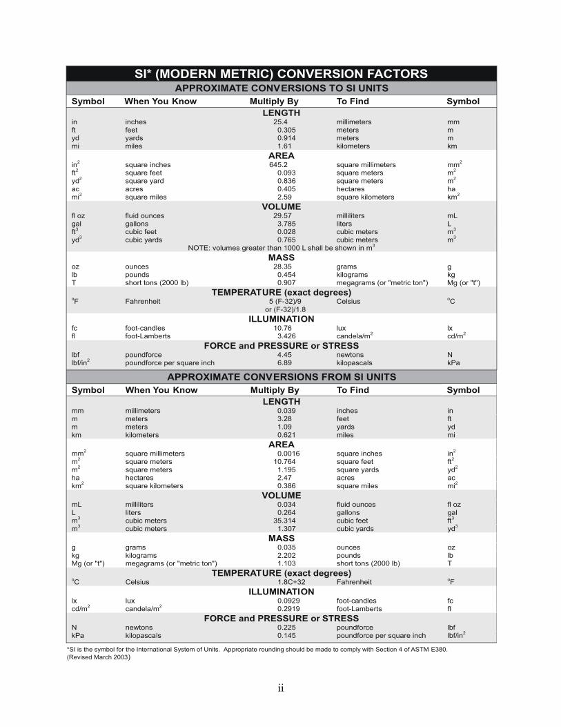
SI* (MODERN METRIC) CONVERSION FACTORS APPROXIMATE CONVERSIONS TO SI UNITS

Symbol When You Know Multiply By To Find Symbol LENGTH

in inches 25.4 millimeters mm ft feet 0.305 meters m yd yards 0.914 meters m mi miles 1.61 kilometers km

AREA in2 square inches 645.2 square millimeters mm2

ft2 square feet 0.093 square meters m2

yd2 square yard 0.836 square meters m2

ac acres 0.405 hectares hami2 square miles 2.59 square kilometers km2

VOLUME fl oz fluid ounces 29.57 milliliters mL gal gallons 3.785 liters L ft3 cubic feet 0.028 cubic meters m3

yd3 cubic yards 0.765 cubic meters m3

NOTE: volumes greater than 1000 L shall be shown in m3

MASS oz ounces 28.35 grams glb pounds 0.454 kilograms kgT short tons (2000 lb) 0.907 megagrams (or "metric ton") Mg (or "t")

TEMPERATURE (exact degrees) oF Fahrenheit 5 (F-32)/9 Celsius oC

or (F-32)/1.8 ILLUMINATION

fc foot-candles 10.76 lux lxfl foot-Lamberts 3.426 candela/m2 cd/m2

FORCE and PRESSURE or STRESS lbf poundforce 4.45 newtons N lbf/in2 poundforce per square inch 6.89 kilopascals kPa

APPROXIMATE CONVERSIONS FROM SI UNITS Symbol When You Know Multiply By To Find Symbol

LENGTHmm millimeters 0.039 inches in m meters 3.28 feet ft m meters 1.09 yards yd km kilometers 0.621 miles mi

AREA mm2 square millimeters 0.0016 square inches in2

m2 square meters 10.764 square feet ft2

m2 square meters 1.195 square yards yd2

ha hectares 2.47 acres ackm2 square kilometers 0.386 square miles mi2

VOLUME mL milliliters 0.034 fluid ounces fl oz L liters 0.264 gallons gal m3 cubic meters 35.314 cubic feet ft3

m3 cubic meters 1.307 cubic yards yd3

MASS g grams 0.035 ounces ozkg kilograms 2.202 pounds lbMg (or "t") megagrams (or "metric ton") 1.103 short tons (2000 lb) T

TEMPERATURE (exact degrees) oC Celsius 1.8C+32 Fahrenheit oF

ILLUMINATION lx lux 0.0929 foot-candles fc cd/m2 candela/m2 0.2919 foot-Lamberts fl

FORCE and PRESSURE or STRESS N newtons 0.225 poundforce lbf kPa kilopascals 0.145 poundforce per square inch lbf/in2

*SI is the symbol for th International System of Units. Appropriate rounding should be made to comply with Section 4 of ASTM E380. e(Revised March 2003)

ii

TABLE OF CONTENTS CHAPTER 1: INTRODUCTION...........................................................................1

LONG-TERM PAVEMENT PERFORMANCE PROGRAM................................................... 1 DATA COLLECTION AT GPS AND SPS SECTIONS ........................................................... 2 DEVICES FOR PROFILE DATA COLLECTION ................................................................... 4 RESEARCH OBJECTIVES ....................................................................................................... 4 ORGANIZATION OF THE REPORT....................................................................................... 5

CHAPTER 2: PROFILING DEVICES USED IN THE LTPP PROGRAM.....7

INERTIAL PROFILERS............................................................................................................ 7 K.J. Law Engineers DNC 690 Profiler ................................................................................... 7 K.J. Law Engineers T-6600 Profiler ....................................................................................... 8 International Cybernetics Corporation Profiler ...................................................................... 9

DIFFERENCES AMONG THE INERTIAL PROFILERS...................................................... 10 Height-Sensor Type and Footprint........................................................................................ 10 Sensor Spacing...................................................................................................................... 10 Number of Sensors................................................................................................................ 10 Location of Height Sensors................................................................................................... 11 Measurement Range of Height Sensors................................................................................ 11 Data Recording Interval........................................................................................................ 12 Data Filtering Methods ......................................................................................................... 12

DIPSTICK................................................................................................................................. 12 MANUALS FOR PROFILER OPERATIONS ........................................................................ 12 COMPUTATION OF ROUGHNESS INDICES ..................................................................... 13

CHAPTER 3: PROFILER COMPARISON STUDIES.....................................15

INTRODUCTION .................................................................................................................... 15 LTPP PROFILER COMPARISON STUDIES......................................................................... 15

Overview............................................................................................................................... 15 Purpose of Comparison Test................................................................................................. 16 Selection of Test Sections..................................................................................................... 17 Collection of Reference Elevation Measurements................................................................ 18 Profiler Data Collection ........................................................................................................ 18 Computation of IRI Values................................................................................................... 19 Analysis of Data from LTPP Comparison Studies ............................................................... 19

LTPP PROFILER VERIFICATION STUDIES....................................................................... 19 OTHER PROFILER COMPARISON/ANALYTICAL STUDIES.......................................... 19

PIARC Comparison .............................................................................................................. 19 Road Profiler User Group Comparisons: 1993 and 1994 ..................................................... 20 LTPP Profile Variability Analysis ........................................................................................ 20

iii

CHAPTER 4: ANALYTICAL PROCEDURES .................................................21 INTRODUCTION .................................................................................................................... 21 ANALYTICAL TECHNIQUES AND SOFTWARE .............................................................. 21

Roughness Profiles................................................................................................................ 21 Power Spectral Density Plots................................................................................................ 24 Data Filtering ........................................................................................................................ 24 Cross Correlation .................................................................................................................. 26 RoadRuf Software................................................................................................................. 28

ANALYTICAL APPROACH .................................................................................................. 29 CHAPTER 5: DATA COLLECTION CHARACTERISTICS AND COMPARISON OF DATA COLLECTED BY LTPP’S PROFILERS ...........31

CHARACTERISTICS OF DATA COLLECTED BY LTPP’S PROFILERS......................... 31 K.J. Law Engineers DNC 690 Profiler ................................................................................. 31 K.J. Law Engineers T-6600 Profiler ..................................................................................... 31 International Cybernetics Corporation Profiler .................................................................... 32

COMPARISON OF K.J. LAW ENGINEERS DNC 690 AND T-6600 PROFILERS ............ 33 Comparison of Profile Data .................................................................................................. 33 Comparison of IRI Values .................................................................................................... 36 Cross Correlation of IRI........................................................................................................ 44 Analysis of Variance and Regression Analysis of IRI.......................................................... 45

COMPARISON OF K.J. LAW ENGINEERS T-6600 AND ICC PROFILERS ..................... 46 Comparison of Profile Data .................................................................................................. 46 Comparison of IRI Values .................................................................................................... 53 Cross Correlation of IRI........................................................................................................ 59 ANOVA and Regression Analysis of IRI............................................................................. 60

EFFECTS OF APPLYING A MOVING AVERAGE ONTO PROFILE DATA .................... 60 Faulted Pavement.................................................................................................................. 61 Effects of Downward Features.............................................................................................. 61 Effects of Sharp Upward Features ........................................................................................ 64 Smooth Asphalt Pavement.................................................................................................... 64

SUMMARY OF THE FINDINGS ........................................................................................... 66 CHAPTER 6: DIFFERENCES BETWEEN DIPSTICK AND PROFILER IRI ......................................................................................................69

INTRODUCTION .................................................................................................................... 69 FACTORS CONTRIBUTING TO DIFFERENCES BETWEEN DIPSTICK AND PROFILER IRI ....................................................................................................................... 69 Sampling Qualities of Dipstick............................................................................................. 69 Variations in the Path Followed by the Profiler.................................................................... 73 Features Recorded by the Profiler That Are Missed or Underestimated by Dipstick .......... 75 Averaging Effects of Profiler Data ....................................................................................... 77 Dipstick Data Errors ............................................................................................................. 78 IRI Computation Procedure for Dipstick Data ..................................................................... 81

iv

DISCUSSION OF DIFFERENCES IN IRI BETWEEN DIPSTICK AND THE PROFILERS ........................................................................................................................... 82

EXPECTED DIFFERENCES BETWEEN DIPSTICK AND PROFILER IRI........................ 88 SUMMARY OF THE FINDINGS ........................................................................................... 90

CHAPTER 7: OTHER FINDINGS FROM ANALYSIS OF THE DATA ......93

INTRODUCTION .................................................................................................................... 93 IRI VALUES COMPUTED USING PROQUAL .................................................................... 93 ACCELEROMETER EFFECTS ON THE K.J. LAW ENGINEERS T-6600 PROFILER DATA ..................................................................................................................................... 94

OBSERVATIONS ON SHORT-WAVELENGTH DATA COLLECTED BY THE K.J. LAW ENGINEERS T-6600 PROFILERS...................................................................... 97 Data from the 2000 Profiler Comparison.............................................................................. 97 Evaluation of Data from the 1998 LTPP Profiler Comparison........................................... 100

IRI DIFFERENCES FOR THE SOUTHERN PROFILER DURING THE 1991 PROFILER COMPARISON .................................................................................................................... 103

SUMMARY OF THE FINDINGS ......................................................................................... 103 CHAPTER 8: CONCLUSIONS AND RECOMMENDATIONS .................. 105

DATA COLLECTED BY INERTIAL PROFILERS............................................................. 105 EFFECT OF APPLYING A MOVING AVERAGE ONTO PROFILE DATA .................... 105 COMPARISON OF THE K.J. LAW ENGINEERS DNC 690 AND T-6600 PROFILERS.. 106 COMPARISON OF THE K.J. LAW ENGINEERS T-6600 AND ICC PROFILERS .......... 106 IRI VALUES .......................................................................................................................... 106 DIFFERENCES IN IRI BETWEEN PROFILERS AND DIPSTICK.................................... 107 REPEATABILITY OF THE K.J. LAW ENGINEERS T-6600 PROFILER ......................... 108 SHORT-WAVELENGTH ERRORS IN DATA COLLECTED BY THE K.J. LAW

ENGINEERS T-6600 PROFILER........................................................................................ 108 Spikes in PSD Plots ............................................................................................................ 108 Western K.J. Law Engineers T-6600 Profiler Data ............................................................ 109

RECOMMENDATIONS FOR IMPROVING CURRENT LTPP DATA COLLECTION AND DATA PROCESSING PROCEDURES ..................................................................... 109

RECOMMENDATIONS ON LTPP PROFILER COMPARISONS ..................................... 110 APPENDIX A: LTPP PROFILER COMPARISON STUDIES..................... 111 APPENDIX B: PROFILER VERIFICATION STUDIES.............................. 131 REFERENCES.................................................................................................... 143

v

LIST OF FIGURES Figure 1. LTPP regions. .................................................................................................................. 3 Figure 2. K.J. Law Engineers DNC 690 profiler with a motor-home body. .................................. 7 Figure 3. K.J. Law Engineers DNC 690 profiler housed in a van. ................................................. 7 Figure 4. K.J. Law Engineers T-6600 profiler................................................................................ 9 Figure 5. ICC MDR 4086L3 profiler.............................................................................................. 9 Figure 6. Height-sensor footprints. ............................................................................................... 11 Figure 7. Schematic view of Dipstick........................................................................................... 13 Figure 8. Roughness of a roadway expressed in 10-m (33-ft) segments. ..................................... 21 Figure 9. Example of a roughness profile..................................................................................... 22 Figure 10. IRI obtained from two repeat runs............................................................................... 23 Figure 11. Roughness profiles at 10-m (33-ft) base length for two runs...................................... 23 Figure 12. Example of a PSD plot. ............................................................................................... 24 Figure 13. Profile recorded by a profiler. ..................................................................................... 25 Figure 14. Profile after being subjected to a 5-m (16-ft) high-pass filter. .................................... 25 Figure 15. Profile after being subjected to a 10-m (33-ft) low-pass filter. ................................... 26 Figure 16. Profile after being subjected to a band-pass filter. ...................................................... 26 Figure 17. Three IRI filtered profiles with an average correlation greater than 0.995. ................ 27 Figure 18. Three IRI filtered profiles with an average correlation of 0.84.(21) ............................. 28 Figure 19. PSD plot of data collected by the K.J. Law Engineers DNC 690 profiler. ................. 31 Figure 20. PSD plot of data collected by the K.J. Law Engineers T-6600 profiler...................... 32 Figure 21. PSD plot of data collected by the ICC profiler............................................................ 33 Figure 22. Data collected by the North Central K.J. Law Engineers DNC 690 and T-6600

profilers at the smooth AC site during the 1996 verification test. ............................................. 34 Figure 23. Data collected by the North Central K.J. Law Engineers DNC 690 and T-6600

profilers at the rough AC site during the 1996 verification test. ............................................... 34 Figure 24. PSD plot of data collected by the K.J. Law Engineers DNC 690 and T-6600

profilers ...................................................................................................................................... 35 Figure 25. PSD plots of K.J. Law Engineers DNC 690 profiler data and ProQual-processed

T-6600 profiler data ................................................................................................................... 36 Figure 26. Relationship between IRI from the K.J. Law Engineers DNC 690 and T-6600

profilers. ..................................................................................................................................... 39Figure 27. Differences in IRI between the K.J. Law Engineers DNC 690 and T-6600 profilers:

All regions.................................................................................................................................. 40 Figure 28. Differences in IRI between the K.J. Law Engineers DNC 690 and T-6600 profilers:

North Atlantic region ................................................................................................................. 41 Figure 29. Differences in IRI between the K.J. Law Engineers DNC 690 and T-6600 profilers:

North Central region .................................................................................................................. 42 Figure 30. Differences in IRI between the K.J. Law Engineers DNC 690 and T-6600 profilers:

Southern region.......................................................................................................................... 43 Figure 31. Differences in IRI between the K.J. Law Engineers DNC 690 and T-6600 profilers:

Western region ........................................................................................................................... 44 Figure 32. Comparison of ICC and K.J. Law Engineers profiles: Western site 320209. ............. 47 Figure 33. Comparison of ICC and K.J. Law Engineers profiles: Western site 069107. ............. 48 Figure 34. Response of the IRI filter. ........................................................................................... 48

vi

Figure 35. PSD plot of 25-mm (1-inch) data collected by the North Central ICC and K.J. Law Engineers profilers at the chip-seal section during the 2002 verification test............ 49

Figure 36. Closeup view of 25-mm (1-inch) profile data collected by North Central ICC and K.J. Law Engineers profilers on a chip-seal pavement.............................................................. 50

Figure 37. Readings taken over a joint by the two profilers......................................................... 52 Figure 38. Profile data obtained by the ICC and K.J. Law Engineers profilers at a concrete site.52 Figure 39. Relationship between IRI from the K.J. Law Engineers and ICC profilers. ............... 54 Figure 40. Differences in IRI between the K.J. Law Engineers and ICC profilers. ..................... 54 Figure 41. Differences in IRI between the K.J. Law Engineers and ICC profilers:

North Atlantic region. ................................................................................................................ 55 Figure 42. Differences in IRI between the K.J. Law Engineers and ICC profilers:

North Central region. ................................................................................................................. 56Figure 43. Differences in IRI between the K.J. Law Engineers and ICC profilers:

Southern region.......................................................................................................................... 58Figure 44. Differences in IRI between the K.J. Law Engineers and ICC profilers:

Western region. .......................................................................................................................... 59 Figure 45. Profile distortion caused by the application of a moving average onto data collected

over a fault. ................................................................................................................................ 61 Figure 46. Profile distortion caused by the application of a moving average onto data collected

over a patched crack................................................................................................................... 62 Figure 47. Profile distortion caused by the application of a moving average onto data collected

over a crack. ............................................................................................................................... 63 Figure 48. Application of a moving average onto data collected for a concrete pavement.......... 64 Figure 49. Application of a moving average onto a profile containing a sharp upward feature. . 65 Figure 50. The 25-mm (1-inch) data and 150-mm (5.9-inch) averaged data from a smooth AC

section. ....................................................................................................................................... 65 Figure 51. Offset profile plot of 25-mm (1-inch) data and averaged 150-mm (5.9-inch) data

collected from a smooth AC pavement...................................................................................... 66 Figure 52. Dipstick response to a sinusoid with a wavelength equal to the footpad spacing of

Dipstick. ..................................................................................................................................... 70 Figure 53. Gain plot of Dipstick. .................................................................................................. 71 Figure 54. An example of aliasing................................................................................................ 72 Figure 55. Roughness profiles for nine runs that show good agreement...................................... 74 Figure 56. Roughness profiles for two profile runs that show variations..................................... 75 Figure 57. Roughness profiles along the left wheelpath for three profilers.................................. 75 Figure 58. Measurement of cracks by a profiler and Dipstick...................................................... 76 Figure 59. Measurement of a downward feature by a profiler and Dipstick. ............................... 77 Figure 60. Illustration of artificial profile used by ProQual for computing IRI. .......................... 78 Figure 61. Left-wheelpath 10-m (33-ft) base-length roughness profiles for profiler and

Dipstick at site 5......................................................................................................................... 79 Figure 62. Left-wheelpath profiles for profiler and Dipstick at site 5. ......................................... 80 Figure 63. Right-wheelpath profiles for profiler and Dipstick at site 1........................................ 80 Figure 64. Roughness profiles for a profiler and Dipstick showing good agreement in roughness

distribution. ................................................................................................................................ 83 Figure 65. Roughness profiles for a profiler and Dipstick showing moderate agreement in

roughness distribution................................................................................................................ 84

vii

Figure 66. Roughness profiles for the case with the lowest cross correlation.............................. 86 Figure 67. Roughness profiles for the case with the highest cross correlation............................. 86 Figure 68. Overlaid right-sensor profiles of the K.J. Law Engineers DNC 690 profiler.............. 95 Figure 69. Overlaid right-sensor profiles of the K.J. Law Engineers T-6600 profiler. ................ 96 Figure 70. Overlaid right-sensor profiles from the K.J. Law Engineers DNC 690 and

T-6600 profilers. ........................................................................................................................ 96 Figure 71. Right-sensor profile data collected by the Western and North Central profilers. ....... 98 Figure 72. PSD plots of the right-sensor data collected by the North Central and Western

profilers at site 2......................................................................................................................... 98 Figure 73. PSD plot of the left-sensor profile data from the North Atlantic profiler. ................ 100 Figure 74. PSD plots of 25-mm (1-inch) right-sensor data from the North Central and Western

profilers. ................................................................................................................................... 101 Figure 75. PSD plots of ProQual-processed right-sensor data from the North Central

and Western profilers............................................................................................................... 102

viii

LIST OF TABLES

Table 1. GPS experiments............................................................................................................... 2 Table 2. SPS experiments. .............................................................................................................. 2 Table 3. Changes in IRI caused by lateral variations in the longitudinal path. ............................ 37 Table 4. IRI values from the 1996 verification test. ..................................................................... 39 Table 5. Results of cross correlation between the K.J. Law Engineers DNC 690 and

T-6600 profilers. ........................................................................................................................ 45 Table 6. Standard deviations of filtered elevation values. ............................................................ 51 Table 7. Results of cross correlation between the K.J. Law Engineers T-6600 and

ICC profilers. ............................................................................................................................. 60 Table 8. IRI values for Dipstick data computed using ProQual and RoadRuf. ............................ 82 Table 9. Results of cross-correlation analysis: Left wheelpath. ................................................... 84 Table 10. Results of cross-correlation analysis: Right wheelpath. ............................................... 85 Table 11. Cross correlation of IRI for North Atlantic and Western profilers............................... 87 Table 12. Differences between the K.J. Law Engineers DNC 690 profiler IRI and

Dipstick IRI................................................................................................................................ 89 Table 13. Differences between the K.J. Law Engineers T-6600 profiler IRI and Dipstick IRI. .. 89 Table 14. Differences between the ICC profiler IRI and Dipstick IRI......................................... 90 Table 15. IRI values computed using ProQual and RoadRuf. ...................................................... 94 Table 16. Comparison of the IRI from the 25-mm (1-inch) data with the IRI from ProQual. ..... 95 Table 17. IRI values along the left wheelpath (1991)................................................................. 112 Table 18. IRI values along the right wheelpath (1991). ............................................................. 113 Table 19. Differences between profiler IRI and Dipstick IRI: Left wheelpath (1991)............... 113 Table 20. Differences between profiler IRI and Dipstick IRI: Right wheelpath (1991). ........... 113 Table 21. Standard deviations of IRI for 80-km/h (50-mi/h) runs: Left wheelpath (1991)........ 114 Table 22. Standard deviations of IRI for 80-km/h (50-mi/h) runs: Right wheelpath (1991)...... 114 Table 23. IRI values along the left wheelpath (1992)................................................................. 116 Table 24. IRI values along the right wheelpath (1992). ............................................................. 116 Table 25. Differences between profiler IRI and Dipstick IRI: Left wheelpath (1992)............... 117 Table 26. Differences between profiler IRI and Dipstick IRI: Right wheelpath (1992). ........... 117 Table 27. Standard deviations of IRI for 80-km/h (50-mi/h) runs: Left wheelpath (1992)........ 117 Table 28. Standard deviations of IRI for 80-km/h (50-mi/h) runs: Right wheelpath (1992)...... 118 Table 29. IRI values along the left wheelpath (1998)................................................................. 120 Table 30. IRI values along the right wheelpath (1998). ............................................................. 120 Table 31. Differences between the profiler IRI and Dipstick IRI: Left wheelpath (1998)......... 120Table 32. Differences between the profiler IRI and Dipstick IRI: Right wheelpath (1998). ..... 121Table 33. Standard deviations of IRI: Left wheelpath (1998). ................................................... 121 Table 34. Standard deviations of IRI: Right wheelpath (1998). ................................................. 121 Table 35. IRI values along the left wheelpath (2000)................................................................. 123 Table 36. IRI values along the right wheelpath (2000). ............................................................. 123 Table 37. Differences between the profiler IRI and the walking profiler IRI (2000)................. 123 Table 38. Standard deviations of IRI: Left wheelpath (2000). ................................................... 124 Table 39. Standard deviations of IRI: Right wheelpath (2000). ................................................. 124 Table 40. IRI values along the left wheelpath (2003)................................................................. 126 Table 41. IRI values along the right wheelpath (2003). ............................................................. 126

ix

Table 42. Differences between the profiler IRI and Dipstick IRI: Left wheelpath (2003)......... 127 Table 43. Differences between the profiler IRI and Dipstick IRI: Right wheelpath (2003). ..... 127 Table 44. Standard deviations of IRI: Left wheelpath (2003). ................................................... 127 Table 45. Standard deviations of IRI: Right wheelpath (2003). ................................................. 128 Table 46. Profiler IRI for 80-km/h (50-mi/h) runs and Dipstick IRI: North Atlantic region. .... 132 Table 47. Differences between the profiler IRI and the Dipstick IRI: North Atlantic region. ... 132 Table 48. Profiler IRI for 80-km/h (50-mi/h) runs and Dipstick IRI: North Central region. ..... 134 Table 49. Differences between the profiler IRI and the Dipstick IRI: North Central region. .... 134 Table 50. Profiler IRI for 80-km/h (50-mi/h) runs and Dipstick IRI: Southern region. ............. 135 Table 51. Differences between the profiler IRI and the Dipstick IRI: Southern region. ............ 136 Table 52. Profiler IRI for 80-km/h (50-mi/h) runs and Dipstick IRI: Western region. .............. 137 Table 53. Differences between the profiler IRI and the Dipstick IRI: Western region. ............. 138 Table 54. IRI values obtained from the 2002 verification study. ............................................... 141

x

ACRONYMS AND ABBREVIATIONS

AC Asphalt Concrete ANOVA Analysis of Variance ARRB Australian Road Research Board DMI Distance Measuring Instrument DOT Department of Transportation FHWA Federal Highway Administration GPS General Pavement Studies ICC International Cybernetics Corporation IRI International Roughness Index LTPP Long-Term Pavement Performance Mn/DOT Minnesota Department of Transportation Mn/ROAD Minnesota Road Research Project NCHRP National Cooperative Highway Research Program PCC Portland Cement Concrete PSD Power Spectral Density RMSVA Root Mean Square Vertical Acceleration RN Ride Number RSC Regional Support Contractor SHRP Strategic Highway Research Program SPS Specific Pavement Studies TxDOT Texas Department of Transportation UMTRI University of Michigan Transportation Research Institute

xi

CHAPTER 1: INTRODUCTION LONG-TERM PAVEMENT PERFORMANCE PROGRAM The Strategic Highway Research Program (SHRP) was a 5-year, $150-million research program that began in 1987. The research areas targeted under SHRP were asphalt, pavement performance, concrete and structures, and highway operations. One aspect of SHRP was the Long-Term Pavement Performance (LTPP) program. The LTPP program was designed as a 20-year study. The first 5 years of the program were administrated by SHRP and, afterwards, administration of the program was transferred to the Federal Highway Administration (FHWA). The objectives of the LTPP program are to: • Evaluate existing design methods. • Develop improved design methods and strategies for rehabilitating existing pavements. • Develop improved design equations for new and reconstructed pavements. • Determine the effects of loading, environment, material properties and variability,

construction quality, and maintenance levels on pavement distress and performance. • Determine the effects of specific design features on pavement performance. • Establish a national long-term pavement database to support SHRP objectives and future

needs. To accomplish these objectives, the LTPP program was divided into two complementary programs. The first program, General Pavement Studies (GPS), uses inservice pavement test sections in either their original design phase or in their first overlay phase. The second program, Specific Pavement Studies (SPS), investigates the effects of specific design features on pavement performance. Under the GPS program, more than 800 test sections were established on inservice pavements in all 50 States and in Canada. Each GPS section is 152.4 meters (m) (500 feet (ft)) long, and is located in the outside traffic lane. The GPS sections are categorized into different experiments based on the pavement type as shown in table 1. The GPS sections generally represent pavements that incorporate materials and structural designs used in standard engineering practices in the United States and Canada. The objective of the GPS program is to use the data collected at the GPS sections to develop improved pavement design procedures. The SPS experiments are designed to study the effects of specific design features on pavement performance. Each SPS experiment consists of multiple test sections. The SPS experiments that were designed for the LTPP program are shown in table 2.

1

Table 1. GPS experiments.

GPS Experiment Description

Number GPS-1 Asphalt Concrete on Granular Base GPS-2 Asphalt Concrete on Stabilized Base GPS-3 Jointed Plain Concrete GPS-4 Jointed Reinforced Concrete GPS-5 Continuously Reinforced Concrete GPS-6 Asphalt Concrete Overlay of Asphalt Pavements GPS-7 Asphalt Overlay of Concrete Pavements GPS-9 Unbonded Concrete Overlay of Concrete Pavements

Table 2. SPS experiments.

SPS Experiment Description

Number SPS-1 Strategic Study of Structural Factors for Flexible Pavements SPS-2 Strategic Study of Structural Factors for Rigid Pavements SPS-3 Preventive Maintenance Effectiveness for Flexible Pavements SPS-4 Preventive Maintenance Effectiveness for Rigid Pavements SPS-5 Rehabilitation of Asphalt Concrete Pavements SPS-6 Rehabilitation of Jointed Concrete Pavements SPS-7 Bonded Concrete Overlay of Concrete Pavements SPS-8 Study of Environmental Factors in the Absence of Heavy Loads SPS-9 Validation of SHRP Asphalt Specifications and Mix Design

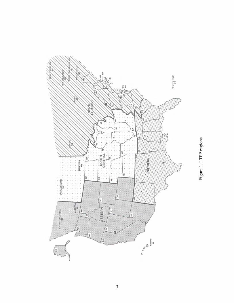
DATA COLLECTION AT GPS AND SPS SECTIONS The GPS and SPS test sections are monitored at regular intervals to collect deflection, profile, and distress data. For purposes of data collection, the United States and the Canadian Provinces have been subdivided into four regions: (1) North Atlantic, (2) North Central, (3) Southern, and (4) Western. Each region is served by a Regional Support Contractor (RSC) who performs data collection at the test sections located within its region. The regional boundaries defining the jurisdiction of each RSC are shown in figure 1. One of the major data collection efforts in the LTPP program is the collection of longitudinal profile data at LTPP test sections. Longitudinal profile data are collected using an inertial profiler (except for test sections located in Alaska, Hawaii, and Puerto Rico, where data are collected using Dipstick®, a hand-operated device manufactured by the Face Company®).

2

Figu

re 1

. LTP

P re

gion

s.

3

Profile data at LTPP test sections are collected along the two wheelpaths. The collected profile data are processed to compute roughness indices such as the International Roughness Index (IRI), Root Mean Square Vertical Acceleration (RMSVA), Slope Variance, and the Mays Index. The computed roughness parameters and the profile data are stored in the LTPP database after undergoing quality control checks. The data in the LTPP database are available to the research community. DEVICES FOR PROFILE DATA COLLECTION Each RSC operates an inertial profiler to collect longitudinal profile data. From the inception of the LTPP program until the end of 1996, profile data at test sections were collected using a model DNC 690 incandescent profiler manufactured by K.J. Law Engineers. In late 1996, each RSC replaced their model DNC 690 profiler with a model T-6600 infrared profiler manufactured by K.J. Law Engineers. In September 2002, each RSC replaced their T-6600 profiler with an International Cybernetics Corporation (ICC) MDR 4086L3 laser profiler. At test sections located in Alaska, Hawaii, and Puerto Rico, longitudinal profile data collection is performed using Dipstick. RESEARCH OBJECTIVES As described previously, data collection at LTPP test sections has been performed using three types of inertial profilers. Differences in the sampling interval, filtering procedures, and sensing devices for these profilers could lead to differences in profiles and smoothness index values among the devices. To ensure that high-quality and repeatable data are collected with each device, it is important to confirm the compatibility of the indices obtained using these devices. An analysis of LTPP profile data and equipment is necessary for quantifying the differences in IRI values among these profiling devices. The end result of this analysis will be an improvement in the quality of future LTPP data collection and an understanding of how to use the current LTPP profile data for analysis. Another useful result is quantification of the tolerances with which these profilers agree so that studies of roughness progression may be done with the knowledge of the differences among the devices. The main objective of this project is to quantify and resolve the differences in the longitudinal profile and roughness indices that are attributable to the different profiling equipment that have been used in the LTPP program. Under this research project, the following activities were carried out to meet the project objective: • Review of reports on LTPP profiler comparison studies that have been performed in the

past and review of other literature on Dipstick testing and profiler comparisons. • Quantification of differences in IRI related to different profiling equipment and

investigation of factors causing differences in IRI among the different inertial profiler types.

4

• Use of data collected for LTPP profiler comparison studies to investigate factors causing differences in IRI obtained from Dipstick and different types of profilers.

• Identification of problems with equipment functionality, and current data collection and

data processing procedures. Provision of recommendations for modifying current data collection and data processing procedures.

• Development of a table listing the expected range of differences among the IRI values

collected using LTPP’s profilers and Dipstick, and provision of recommendations for recalculation of IRI based on the findings.

• Preparation of a final report that describes the analyses performed, findings from the

analyses, and recommendations for improvements in LTPP data collection and processing procedures.

All analyses were performed using the data that were collected during LTPP profiler comparison studies. ORGANIZATION OF THE REPORT Chapter 2 presents a description of profiling devices that have been used in the LTPP program to collect longitudinal profile data. Chapter 3 presents an overview of LTPP profiler comparison studies that have been performed since the inception of the LTPP program. Chapter 4 presents a description of analytical procedures that were used in this research project to analyze profile data. Chapter 5 presents a description of the data collection characteristics of LTPP’s profilers and a comparison of the devices. Chapter 6 presents the factors that can cause differences in IRI obtained from profilers and Dipstick. Chapter 7 presents several other findings from analysis of the profile data obtained from LTPP profiler comparison studies. Chapter 8 presents conclusions and recommendations for improvements to current procedures used in the collection and processing of profile data in the LTPP program.

5

CHAPTER 2: PROFILING DEVICES USED IN THE LTPP PROGRAM

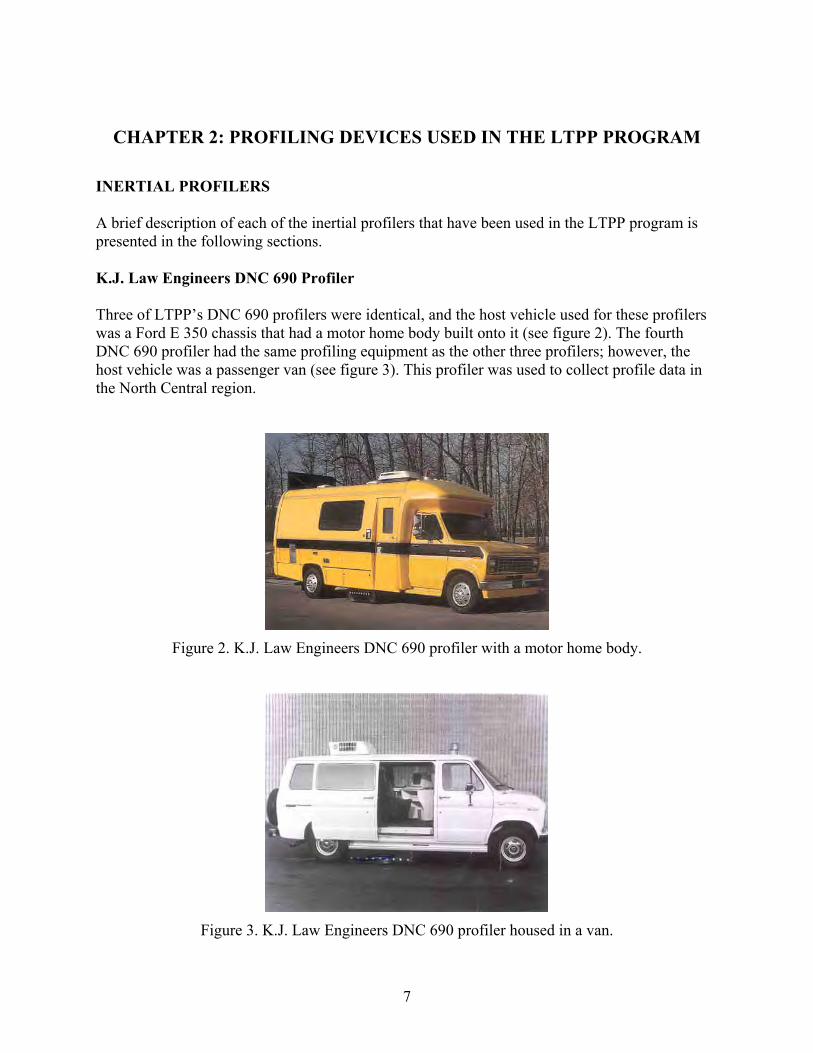
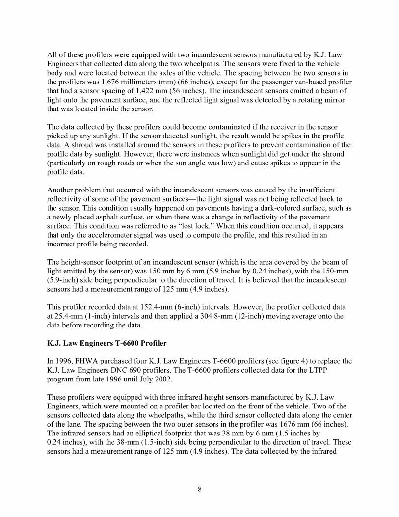
INERTIAL PROFILERS A brief description of each of the inertial profilers that have been used in the LTPP program is presented in the following sections. K.J. Law Engineers DNC 690 Profiler Three of LTPP’s DNC 690 profilers were identical, and the host vehicle used for these profilers was a Ford E 350 chassis that had a motor home body built onto it (see figure 2). The fourth DNC 690 profiler had the same profiling equipment as the other three profilers; however, the host vehicle was a passenger van (see figure 3). This profiler was used to collect profile data in the North Central region.

Figure 2. K.J. Law Engineers DNC 690 profiler with a motor home body.

Figure 3. K.J. Law Engineers DNC 690 profiler housed in a van.

7

All of these profilers were equipped with two incandescent sensors manufactured by K.J. Law Engineers that collected data along the two wheelpaths. The sensors were fixed to the vehicle body and were located between the axles of the vehicle. The spacing between the two sensors in the profilers was 1,676 millimeters (mm) (66 inches), except for the passenger van-based profiler that had a sensor spacing of 1,422 mm (56 inches). The incandescent sensors emitted a beam of light onto the pavement surface, and the reflected light signal was detected by a rotating mirror that was located inside the sensor. The data collected by these profilers could become contaminated if the receiver in the sensor picked up any sunlight. If the sensor detected sunlight, the result would be spikes in the profile data. A shroud was installed around the sensors in these profilers to prevent contamination of the profile data by sunlight. However, there were instances when sunlight did get under the shroud (particularly on rough roads or when the sun angle was low) and cause spikes to appear in the profile data. Another problem that occurred with the incandescent sensors was caused by the insufficient reflectivity of some of the pavement surfaces—the light signal was not being reflected back to the sensor. This condition usually happened on pavements having a dark-colored surface, such as a newly placed asphalt surface, or when there was a change in reflectivity of the pavement surface. This condition was referred to as “lost lock.” When this condition occurred, it appears that only the accelerometer signal was used to compute the profile, and this resulted in an incorrect profile being recorded. The height-sensor footprint of an incandescent sensor (which is the area covered by the beam of light emitted by the sensor) was 150 mm by 6 mm (5.9 inches by 0.24 inches), with the 150-mm (5.9-inch) side being perpendicular to the direction of travel. It is believed that the incandescent sensors had a measurement range of 125 mm (4.9 inches). This profiler recorded data at 152.4-mm (6-inch) intervals. However, the profiler collected data at 25.4-mm (1-inch) intervals and then applied a 304.8-mm (12-inch) moving average onto the data before recording the data. K.J. Law Engineers T-6600 Profiler In 1996, FHWA purchased four K.J. Law Engineers T-6600 profilers (see figure 4) to replace the K.J. Law Engineers DNC 690 profilers. The T-6600 profilers collected data for the LTPP program from late 1996 until July 2002. These profilers were equipped with three infrared height sensors manufactured by K.J. Law Engineers, which were mounted on a profiler bar located on the front of the vehicle. Two of the sensors collected data along the wheelpaths, while the third sensor collected data along the center of the lane. The spacing between the two outer sensors in the profiler was 1676 mm (66 inches). The infrared sensors had an elliptical footprint that was 38 mm by 6 mm (1.5 inches by 0.24 inches), with the 38-mm (1.5-inch) side being perpendicular to the direction of travel. These sensors had a measurement range of 125 mm (4.9 inches). The data collected by the infrared

8

height sensors were not affected by ambient light. These profilers recorded profile data at 25-mm (l-inch) intervals.

Figure 4. K.J. Law Engineers T-6600 profiler.

International Cybernetics Corporation Profiler In July 2002, FHWA purchased four new ICC MDR 4086L3 profilers (see figure 5) to replace the K.J. Law Engineers T-6600 profilers. The ICC profilers began collecting profile data for the LTPP program in August 2002, and currently are used to collect profile data.

Figure 5. ICC MDR 4086L3 profiler.

These profilers were equipped with three Selcom® Systems laser sensors mounted on a profiler bar located on the front of the vehicle. Two sensors collect data along the wheelpaths, while the third sensor collects data along the center of the lane. The spacing between the two outer sensors is 1676 mm (66 inches). The footprint of a laser sensor is circular, and has a diameter of about 1.5 mm (0.06 inches). The laser sensors have a measurement range of 200 mm (7.9 inches). The readings obtained by the laser sensors are not affected by ambient light. The ICC profilers do not record profile data, but rather they record in a file the signals measured by the height sensors and the accelerometers, and the distance data from the distance measuring instrument (DMI). After

9

data collection has been completed, a computer program is used to generate profile data at 25-mm (l-inch) intervals. DIFFERENCES AMONG THE INERTIAL PROFILERS Several differences among the three types of inertial profilers that have been used to collect profile data for the LTPP program are: • Height-sensor type and footprint. • Sensor spacing. • Number of sensors. • Location of height sensors. • Measurement range of height sensors. • Data recording interval. • Data filtering methods. Height-Sensor Type and Footprint The DNC 690, T-6600, and ICC profilers were equipped with incandescent sensors, infrared sensors, and laser sensors, respectively. The height-sensor data collected by the DNC 690 profiler could get contaminated by sunlight getting into the sensor through the shroud covering the sensors. The data collection capabilities of the infrared sensors on the T-6600 profiler and the laser sensors on the ICC profilers were not affected by ambient light. Another problem with the DNC 690 profilers was the occurrence of lost lock. This problem did not occur in either the T-6600 profilers or the ICC profilers. There were differences in the height-sensor footprint size among the three profilers. The DNC 690 profilers had a footprint size of 150 mm by 6 mm (5.9 inches by 0.24 inches); the 150-mm (5.9-inch) side was perpendicular to the direction of travel. The T-6600 profilers had an elliptical footprint that was 38 mm by 6 mm (1.5 inches by 0.24 inches); the 38-mm (1.5-inch) side was perpendicular to the direction of travel. The ICC profilers were equipped with laser height sensors that had a circular footprint of about 1.5 mm (0.06 inches) in diameter. Figure 6 shows the relative size of the sensor footprints for the three height sensors. Sensor Spacing The spacing between the two outer sensors for all three profilers was 1,676 mm (66 inches), except for the DNC 690 profiler operated by the North Central region. This profiler had a sensor spacing of 1,422 mm (56 inches). Number of Sensors The DNC 690 profilers were equipped with two height sensors for collecting profile data along the wheelpaths. The T-6600 profilers and the ICC profilers had three sensors for collecting profile data (two sensors collected data along the wheelpaths, and the third sensor was located at the midpoint between the two outer sensors).

10

INCANDESCENT INFRARED LASER

1 inch = 25.4 mm

Figure 6. Height-sensor footprints. Location of Height Sensors In the DNC 690 profilers, the height sensors were located midway between the two axles of the vehicle. The sensors in the T-6600 profilers and the ICC profilers were housed inside a sensor bar that was mounted on the front of the vehicle. Measurement Range of Height Sensors The ICC profilers were equipped with Selcom laser sensors that had a measurement range of 200 mm (7.9 inches). The T-6600 profilers that were equipped with infrared sensors had a measurement range of 125 mm (4.9 inches). It is believed that the incandescent sensors that were used on the DNC 690 profilers had a similar measurement range. A National Cooperative Highway Research Program (NCHRP) study that analyzed data from roads having a roughness of up to 4.5 meters per kilometer (m/km) (285 inches per mile (inches/mi)) found that the range of vertical movement that was expected in a vehicle between the axles (where the sensors on the DNC 690 profiler were located) was well within the measurement range of the sensors on the DNC 690 profiler.(1) Therefore, it is unlikely that the height sensors on the DNC 690 profiler exceeded the measurement range while collecting data. On a road with a given roughness value, the range of movement that is experienced by the profiler bar that is located on the front of the vehicle is much more than the movement that occurs in the vehicle body between the axles. Therefore, on any given road, the height sensors of the T-6600 profiler that were mounted on the front profiler bar measured much more movement than that measured by the height sensors on the DNC 690 profiler. There is a possibility that the measurement range of the height sensors on the T-6600 profiler may have been exceeded at extremely rough locations. If this occurred, it is believed that the reading obtained at the cutoff limit of the height sensor was used to compute the profile at that location. The 200-mm (7.9-inch) height-sensor range for the ICC profilers is expected to be sufficient for collecting data on rough LTPP sections without the height sensors exceeding the measurement range.

11

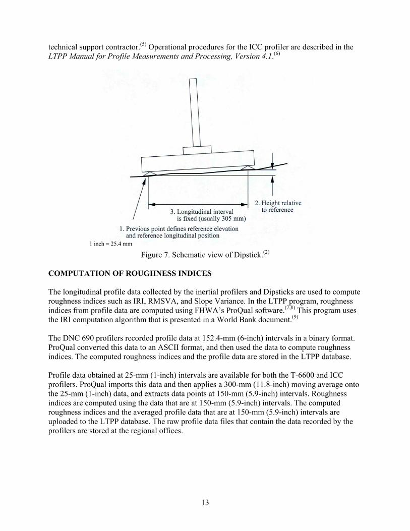
Data Recording Interval The DNC 690 profilers collected profile data at 25.4-mm (1-inch) intervals, and then applied a 304.8-mm (12-inch) moving average onto the data and recorded the data at 152.4-mm (6-inch) intervals. The T-6600 profilers recorded profile data at 25-mm (1-inch) intervals. The ICC profilers do not record profile data; however, they record data obtained from the height sensors, accelerometers, and DMI. It is possible to obtain profile data at 25-mm (1-inch) intervals from these data. Data Filtering Methods Details about the filters used in the computation of the profile data for all three profiler types are not available. The manufacturers of the profilers consider this information to be proprietary. It is possible that the filtering methods used with the DNC 690 and T-6600 profilers may be similar, since the same manufacturer built both of these profilers. Differences in the filtering techniques used in the K.J. Law Engineers profilers and the ICC profilers are expected. A 100-m (328-ft) upper-wavelength cutoff filter is applied to the data obtained from the T-6600 and ICC profilers. The data collected by the DNC 690 profiler were subjected to a 91-m (300-ft) upper-wavelength cutoff filter. DIPSTICK In the LTPP program, longitudinal profile data collection at the test sections located in Alaska, Hawaii, and Puerto Rico is performed using Dipstick, a hand-operated device manufactured by the Face Company. Dipstick has a digital inclinometer that measures the elevation difference between the two footpads (see figure 7).(2) The diameter of the footpads of the Dipsticks used in the LTPP program is approximately 32 mm (1.25 inches). The spacing between the centers of the two footpads is 304.8 mm (12 inches). Dipstick is walked along a test section, and at each position it displays the elevation difference between the two footpads, which is recorded in a data collection form. The individual readings are then added to get the elevation profile. Dipstick is used during LTPP profiler comparisons to obtain reference elevations along the two wheelpaths at the test sections. In 1989, the Center for Transportation Research at the University of Texas at Austin investigated the ability of Dipstick to measure road profiles.(3) This investigation showed that when properly calibrated and operated, Dipstick could give profiles as good as those from rod-and-level surveys, but at a fraction of the time and cost. MANUALS FOR PROFILER OPERATIONS Manuals have been developed that document the operational procedures to be followed when measuring pavement profiles for the LTPP program using an inertial profiler or Dipstick. These manuals cover field testing procedures, data collection procedures, calibration of equipment, record keeping, and maintenance of equipment. The operational procedures for the DNC 690 profiler are documented in a SHRP report (report no. SHRP-P-378).(4) The operational procedures for the T-6600 profiler are contained in a legacy document written by the LTPP

12

technical support contractor.(5) Operational procedures for the ICC profiler are described in the LTPP Manual for Profile Measurements and Processing, Version 4.1.(6)

Figure 7. Schematic view of Dipstick.(2)

OMPUTATION OF ROUGHNESS INDICES

he longitudinal profile data collected by the inertial profilers and Dipsticks are used to compute

he DNC 690 profilers recorded profile data at 152.4-mm (6-inch) intervals in a binary format.

rofile data obtained at 25-mm (1-inch) intervals are available for both the T-6600 and ICC nto

the

1 inch = 25.4 mm

C Troughness indices such as IRI, RMSVA, and Slope Variance. In the LTPP program, roughness indices from profile data are computed using FHWA’s ProQual software.(7,8) This program usesthe IRI computation algorithm that is presented in a World Bank document.(9)

TProQual converted this data to an ASCII format, and then used the data to compute roughness indices. The computed roughness indices and the profile data are stored in the LTPP database. Pprofilers. ProQual imports this data and then applies a 300-mm (11.8-inch) moving average othe 25-mm (1-inch) data, and extracts data points at 150-mm (5.9-inch) intervals. Roughness indices are computed using the data that are at 150-mm (5.9-inch) intervals. The computed roughness indices and the averaged profile data that are at 150-mm (5.9-inch) intervals are uploaded to the LTPP database. The raw profile data files that contain the data recorded by profilers are stored at the regional offices.

13

When computing IRI values from the Dipstick data, the following procedure is used in ProQual: 1. Sum the individual Dipstick readings to obtain the elevation profile of a wheelpath. 2. Rotate the profile for a wheelpath by 180 degrees so that an additional length of 152.4 m

(500 ft) is available before the start of the section. 3. Apply the long-wavelength cutoff filter that is used in the profiler to filter the data so that

wavelengths greater than 100 m (328 ft) are removed. 4. Extract the filtered profile from the start of the test section to the end of the test section. 5. Compute roughness indices using this filtered profile.

14

CHAPTER 3: PROFILER COMPARISON STUDIES

INTRODUCTION Studies have been conducted at regular intervals to compare the output from the four LTPP profilers. For each study, several test sections were laid out, and reference profile measurements along each wheelpath were obtained using Dipstick. Thereafter, profile measurements were performed on the test sections by the profilers. The primary method for checking if the profilers were functioning accurately was to compare the IRI values computed from Dipstick data with the values computed from the data obtained from the profilers. The repeatability of the profilers was evaluated by analyzing the standard deviations of the IRI, which were computed using the IRI values obtained from repeat measurements on a test section. In the profiler comparison studies that have been performed since 1998, in addition to comparing the IRI values, profiles obtained by the profilers were compared to evaluate profiler repeatability and reproducibility. The details of these comparison tests are presented later in this chapter. Whenever FHWA purchased new profilers, the profilers underwent rigorous testing to ensure that they met the requirements that were specified in the contract documents. After each regional contractor took delivery of a new profiler, a comparison of the new profiler and the old profiler was performed in each region before collecting data with the new profiler. The purpose of these verification tests was to compare the output from the old and the new profilers. Details about these verification tests are presented later in this chapter. In this research project, a literature review was also performed to gather information on other profiler comparison studies that have been performed in the past. The results of this literature review are presented later in this chapter. LTPP PROFILER COMPARISON STUDIES Overview The following six LTPP profiler comparison studies have been held since the start of the LTPP program: • 1990: Austin, TX. • 1991: Ann Arbor, MI. • 1992: Ames, IA. • 1998: Urbana, IL. • 2000: College Station, TX. • 2003: Minnesota Road Research Project (Mn/ROAD) of the Minnesota Department of

Transportation (Mn/DOT). This section presents a brief description of the following activities related to an LTPP profiler comparison: (1) purpose of comparison test, (2) selection of test sections, (3) collection of

15

reference elevation measurements, (4) profiler data collection, (5) computation of IRI values, and (6) analysis of data from LTPP comparison studies. Purpose of Comparison Test The purpose of performing a comparison test of the four LTPP profilers is to ensure that the profilers are collecting accurate, repeatable, and reproducible data. Currently, the following analyses are performed on the data collected during a comparison test:(6)

• Evaluation of the static accuracy of the profiler height sensors: Performed before data

collection, this test checks the static accuracy of the height sensors using a set of blocks to determine whether the readings are within a specified tolerance.

• Evaluation of the results from the bounce test: The bounce test determines whether the

height-sensor readings and accelerometer readings are canceling each other. The results of this test for each of the four profilers are compared to determine whether all four profilers are providing similar results.

• Evaluation of the accuracy of the DMI: Performed before data collection, this test

determines whether the DMI meets specified bias and precision criteria. A 300-m- (984-ft-) long section is laid out to perform this test.

• Evaluation of the repeatability of the IRI values obtained by the profilers and a

comparison of the IRI values obtained by profilers with those obtained using Dipstick: The IRI values obtained from the repeat runs of a profiler on a test section are used to evaluate the precision (repeatability) of a profiler. The IRI values are also used to evaluate the bias of a profiler with respect to Dipstick. For comparison studies that have been performed since 1998, the following precision and bias criteria have been evaluated: (1) determination of whether the precision of the IRI along a wheelpath (obtained by computing the standard deviations of the IRI for the repeat profiler runs) is less than 0.04 m/km (2.5 inches/mi), and (2) determination of whether the difference in IRI for a wheelpath between the average profiler IRI (which is calculated by averaging IRI obtained from the five profiler runs) and the Dipstick IRI is within ±0.16 m/km (±10 inches/mi).

• Evaluation of the repeatability of the profile data: The point-to-point repeatability for

each profiler along each wheelpath is computed to evaluate the repeatability of the profile data.

• Comparison of the profile data obtained by the four profilers: One representative run for

each profiler is selected for a test section and overlaid profile plots for each wheelpath at each test section are prepared to compare the data collected by the four profilers.

For comparison tests performed before 1998, an evaluation of the profile data was not performed; the analysis of the data was confined to IRI values.

16

Selection of Test Sections The current LTPP procedures for performing a profiler comparison indicate that five test sections, which satisfy the following criteria, should be selected:(6)

• Section 1: Smooth Asphalt: Asphalt concrete (AC) pavement with an average IRI for the

two wheelpaths of less than 1.6 m/km (101 inches/mi). • Section 2: Rough Asphalt: AC pavement with an average IRI for the two wheelpaths of

greater than 2.2 m/km (139 inches/mi).

• Section 3: Smooth Concrete: Jointed portland cement concrete (PCC) pavement with an average IRI for the two wheelpaths of less than 1.6 m/km (101 inches/mi).

• Section 4: Rough Concrete: Jointed PCC pavement with an average IRI for the two

wheelpaths of greater than 2.2 m/km (139 inches/mi). • Section 5: Chip-sealed section. The comparison study performed in 1990 used six test sections, the studies in 1991 and 1992 used eight test sections, the study in 1998 used four test sections, and the studies in 2000 and 2003 used five test sections. The following guidelines are specified for selecting test sections:(6)

• Each test section should be 152.4 m (500 ft) in length, with the beginning and end

marked. • The test sections should be located on flat, tangential sections that have sufficient length

at each end to allow for acceleration to a constant speed before the section and safe deceleration past its end.

• The speed limit of the roadway containing the test sections should be at least

80 kilometers per hour (km/h) (50 miles per hour (mi/h)). • The test sections should have a marked outside lane-edge stripe that can be used as a

lateral reference when profiling the test section. • The AC sections should not be concrete sections that have been overlaid with asphalt. • Where possible, test sections should be located within a centralized locale, with short

travel distances between each test section to reduce travel time.

17

Collection of Reference Elevation Measurements Dipstick has been used to collect reference elevation data for all profiler comparison studies, except for the study in 2000. In the 2000 study, the reference profile measurements were obtained using an Australian Road Research Board (ARRB) walking profiler. In the 1992 comparison, rod-and-level measurements were obtained in addition to Dipstick measurements. Dipstick measurements are performed along both wheelpaths at all test sections. The current procedures for performing Dipstick measurements are outlined in the LTPP Manual for Profile Measurements and Processing.(6) As described in this document, Dipstick data collection from a test section is performed according to the following sequence: 1. Start data collection from the beginning of the section along the right wheelpath. 2. When the end of the section is reached, go across the lane toward the left wheelpath. 3. Perform measurements along the left wheelpath toward the beginning of the section. 4. After reaching the start of the section, go across the lane and terminate data collection at

the right wheelpath. It is not known whether this procedure for Dipstick data collection was followed when data were collected for the 1990 study. However, this procedure for Dipstick data collection was used for all other profiler comparison studies, except for the study performed in 1991 in Michigan. In the Michigan study, Dipstick measurements were first made along a wheelpath from the beginning of the section to the end of the section and, thereafter, measurements were made along the same path from the end of the section to the beginning of the section. This resulted in two profiles being available for each wheelpath. (Note: This was the Dipstick measurement procedure used in the LTPP program at that time.) Dipstick measurements on PCC test sections were performed in the afternoon, at the same approximate time of day as expected for the collection of profiler data for all comparison studies. This procedure was followed to avoid the slab curling effects that may be present in the PCC pavements in the morning. Profiler Data Collection Current test procedures indicate that data collection at the test sections should be performed at a test speed of 80 km/h (50 mi/h).(6) Data collection at PCC sections was performed in the afternoon, at the same approximate time of day as when Dipstick data were collected at the sections. At each test section, each profiler collects a set of measurements following the normal operating procedures that are used during data collection at LTPP sections. During the 1990 profiler comparison, profile testing was performed at test speeds of 56 and 80 km/h (35 and 50 mi/h). In the profiler comparison studies that were performed in 1991 and 1992, profile testing was performed at test speeds of 64 and 80 km/h (40 and 50 mi/h). For all other comparison studies, profile testing was performed only at 80 km/h (50 mi/h).

18

The left wheelpath for all test sections was marked using paint dots for the profiler comparisons that were conducted in 1990 and 1991. In these studies, the profiler driver was asked to align the vehicle along the left wheelpath when profiling the test sections. In the 2000 comparison, the wheelpaths of two sections were marked with paint dots. In the 2003 comparison, both wheelpaths on all test sections were marked with paint dots. The location of the wheelpaths was not marked for the comparisons that were held in 1992 and 1998. In these studies, the profiler driver judged the location of the wheelpaths and aligned the profiler along the wheelpaths when profiling the test sections. Computation of IRI Values The computation of IRI values from the profiler data was performed by each region using the ProQual software.(7,8) The number of runs that were used in the analysis for the different comparison studies was either five or six. Each RSC selected the profile runs that were to be used in the analysis from all available repeat runs. Each RSC prepared a table that included the left- and right-wheelpath IRI values for all selected runs and submitted the table and a brief report to FHWA and its technical support contractor. Analysis of Data from LTPP Comparison Studies The analysis of data obtained from the LTPP profiler comparison studies has been performed by the LTPP technical support contractor. Reports documenting the analyses and findings for all profiler comparison studies are available. (See references 10, 11, 12, 13, 14, and 15.) Summaries of the findings from each profiler comparison study are presented in appendix A. LTPP PROFILER VERIFICATION STUDIES Profiler equipment changes occurred in the LTPP program in 1996 and 2002. In 1996, each RSC replaced their K.J. Law Engineers DNC 690 profiler with a K.J. Law Engineers T-6600 profiler. In 2002, each RSC replaced their T-6600 profiler with an ICC MDR 4086L3 profiler. On each of these occasions, after accepting delivery of the new profiler, each RSC performed a comparison of the old and new profilers before collecting data with the new profiler. Details and findings from these two verification studies are presented in appendix B. OTHER PROFILER COMPARISON/ANALYTICAL STUDIES A literature review was performed to gather information on other studies that have been performed to compare IRI from profilers and reference devices. The purpose of obtaining information about other studies was to determine if they contained any explanations regarding the differences in IRI between inertial profilers and reference devices that could be useful for this research project. In addition, reports on other studies that have analyzed LTPP profile data were reviewed. PIARC Comparison

19

In 1998, World Road Association (PIARC) Committee C1 on Surface Characteristics conducted a global experiment to investigate the performance of various high-speed profiling equipment.(16) Test sections were established in the United States, Japan, and Europe (The Netherlands and Germany). Reference profile measurements at the test sections were conducted using Dipstick and the ARRB walking profiler. The number of high-speed profilers that performed measurements in the United States, Japan, and Europe were 4, 7, and 25, respectively. The profilers that took measurements at the test sections in the United States generally showed good agreement in IRI. However, there was wide variability in the IRI values that were obtained by the different profilers at the test sections located in Japan and Europe. In addition, there were some large discrepancies in the IRI values obtained from the reference devices and the high-speed profilers at many sections. The causes of the differences in IRI were not investigated in this project. Road Profiler User Group Comparisons: 1993 and 1994 Four regional test centers were used for these studies performed in 1993 and 1994—Pennsylvania, South Dakota, Nevada, and Mississippi.(17,18) Eight test sections were used at each regional center, except for Nevada, where six test sections were used. Dipstick measurements were obtained at all test sections. LTPP’s DNC 690 profilers were used in these two comparisons. An evaluation of the results indicated that at each of the regional test centers, LTPP’s profilers were among the profilers that best matched the Dipstick IRI. LTPP Profile Variability Analysis This study visually reviewed all LTPP profile data that were collected between June 1989 and October 1997 for saturation spikes, lost lock, shifted start, wrong location, out of study, and other equipment- and operator-related problems.(19) The data for the review were obtained from the LTPP database. The profile data for the period under review were collected by the DNC 690 profilers, except for a few data sets that were collected by the T-6600 profilers. The profiles that exhibited problems were divided into two groups—reparable and irreparable profiles. Reparable profiles included profiles with saturation spikes that were not marked. These data were reprocessed, and the IRI values in the LTPP database were updated. Data that exhibited problems that could not be repaired were deleted from the LTPP database.

20

CHAPTER 4: ANALYTICAL PROCEDURES

INTRODUCTION This section describes the analytical techniques and software that were used in this research project, and the overall approach that was used to analyze data collected for the various LTPP profiler comparison and verification studies. The following analytical techniques/software were used for data analysis: • Roughness profiles. • Power spectral density (PSD) plots. • Data filtering. • Cross correlation. • Road Profile Analysis Software (RoadRuf™).1 ANALYTICAL TECHNIQUES AND SOFTWARE Roughness Profiles The roughness of a section of roadway can be expressed by the IRI, which indicates the average roughness for that road section. However, the roughness within this section of roadway can vary. For example, consider a 100-m- (328-ft-) long section of roadway that has a roughness of 1.23 m/km (6.5 ft/mi). This road section can be divided into 10 equidistant segments, where the length of each segment is 10 m (33 ft). Figure 8 shows the roughness of each of these 10-m (33-ft) segments.

0.00.20.40.60.81.01.21.41.6

1 2 3 4 5 6 7 8 9 10Segment Number

IRI (

m/k

m)

1 m/km = 5.28 ft/mi

Figure 8. Roughness of a roadway expressed in 10-m (33-ft) segments.

1 Initially funded by FHWA, this software was developed by the University of Michigan’s Transportation Research Institute.

21

As shown in this figure, the roughness values for the 10-m (33-ft) segments are variable, with segment 1, which has an IRI of 1.42 m/km (7.5 ft/mi), having the highest roughness, and segment 9, which has an IRI of 1.01 m/km (5.3 ft/mi), having the lowest roughness. Instead of using a single value to characterize the roughness of a roadway, a roughness profile can be used to show how roughness varies with distance along the roadway. Figure 9 shows a roughness profile based on a 10-m (33-ft) base length for the same section of roadway whose roughness distribution was shown in figure 8. In figure 9, the roughness value for a specific location is the average roughness over a 10-m (33-ft) length (i.e., the base length of the roughness profile) that is centered at that location. For example, the roughness shown at a distance of 25 m (82 ft) is the average roughness from 20 to 30 m (66 to 98 ft). The highest roughness value in the roughness profile occurs at a distance of 50 m (164 ft), and, therefore, the 10-m (33-ft) stretch of the road that has the highest roughness is between 45 and 55 m (148 and 181 ft). A roughness profile can be constructed for any base length. A detailed description of roughness profiles is presented by Sayers.(20)

0.00.20.40.60.81.01.21.41.61.8

0 20 40 60 80 100Distance (m)

IRI (

m/k

m)

1 m = 3.28 ft. 1 m/km = 5.28 ft/mi

Figure 9. Example of a roughness profile. When evaluating the IRI repeatability of a profiler, or when comparing IRI values obtained by different profilers, an evaluation of roughness profiles provides much more information than just evaluating the IRI value that is obtained for the entire road section. For example, consider the following case where two repeat runs were conducted by a profiler (not LTPP’s profiler) on a test section that was 180 m (590 ft) long. The left-wheelpath IRI values for the two runs were 1.66 and 1.63 m/km (105 and 103 inches/mi). The IRI values obtained for the two repeat runs were very similar, which seems to indicate that the profiler is capable of collecting repeatable data. Figure 10 shows the IRI values for the two runs reported at 10-m (33-ft) intervals. This figure shows that at some segments, there was a considerable difference between the IRI values obtained for the two runs. However, averaging IRI over the 152.4-m- (500-ft-) long section caused these variations to smooth out and gave an overall IRI value for the two repeat runs that was very similar to the individual value for each run.

22

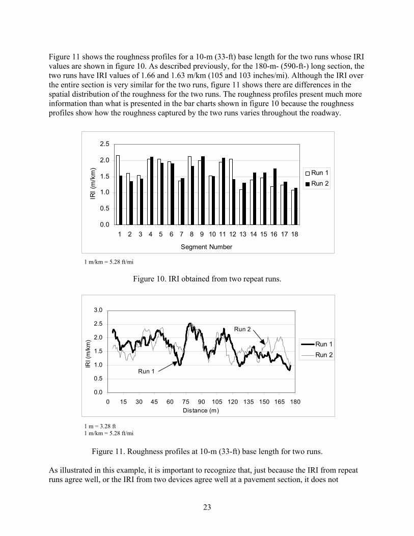
Figure 11 shows the roughness profiles for a 10-m (33-ft) base length for the two runs whose IRI values are shown in figure 10. As described previously, for the 180-m- (590-ft-) long section, the two runs have IRI values of 1.66 and 1.63 m/km (105 and 103 inches/mi). Although the IRI over the entire section is very similar for the two runs, figure 11 shows there are differences in the spatial distribution of the roughness for the two runs. The roughness profiles present much more information than what is presented in the bar charts shown in figure 10 because the roughness profiles show how the roughness captured by the two runs varies throughout the roadway.

0.0

0.5

1.0

1.5

2.0

2.5

1 2 3 4 5 6 7 8 9 10 11 12 13 14 15 16 17 18

Segment Number

IRI (

m/k

m)

Run 1Run 2

Figure 10. IRI obtained from two repeat runs.

1 m = 3.28 ft 1 m/km = 5.28 ft/mi

1 m/km = 5.28 ft/mi

0.0

0.5

1.0

1.5

2.0

2.5

3.0

0 15 30 45 60 75 90 105 120 135 150 165 180Distance (m)

IRI (

m/k

m) Run 1

Run 2

Run 1

Run 2

Figure 11. Roughness profiles at 10-m (33-ft) base length for two runs. As illustrated in this example, it is important to recognize that, just because the IRI from repeat runs agree well, or the IRI from two devices agree well at a pavement section, it does not

23

necessarily mean that the two devices are collecting similar profile data. Roughness profiles can be used to determine whether repeat runs from a profiler or profile runs from different devices are giving a similar spatial distribution of IRI along the section. Power Spectral Density Plots A road profile encompasses a spectrum of sinusoidal wavelengths. A PSD function is a statistical representation of the importance of the various wavelengths contained in the profile.(2) The PSD function of the profile slope best shows the differences in the roughness properties because the basic spectrum of roughness over the wave numbers is more uniform.(2) In this research project, PSD plots that use the profile slope were used in the analyses. Figure 12 shows an example of a PSD plot of a road profile. This plot presents a view of the distribution of the wavelengths that are contained within the road profile. The x-axis of the PSD plot represents the wave number. The wave number is the inverse of the wavelength. If prominent wavelengths are present in a profile, such wavelengths will show up as dominant spikes in the PSD plot.

1 cycle/m = 0.3 cycle/ft 1 m/cycle = 3 ft/cycle

Figure 12. Example of a PSD plot. Data Filtering The profiles obtained by the T-6600 and ICC profilers have been filtered with a 100-m (328-ft) upper-wavelength cutoff filter, while the data obtained by the DNC 690 profilers have been filtered with a 91-m (300-ft) upper-wavelength cutoff filter. The profile data can be further filtered during data analysis to look at details within the profile. The types of filters that are commonly used in analyses are high-pass filters, low-pass filters, and band-pass filters. A high-pass filter removes wavelengths greater than a specified value. A low-pass filter removes wavelengths less than a specified value. A band-pass filter keeps the wavelengths within a specified waveband and removes all other wavelengths. The following example illustrates the application of filtering techniques to profile data. Figure 13 shows a plot of a typical profile that was obtained from LTPP’s T-6600 profiler. Figures 14, 15,

24

and 16, respectively, show this profile after it has been subjected to a 5-m (16-ft) high-pass filter, a 10-m (33-ft) low-pass filter, and a band-pass filter that has a lower wavelength of 5 m (16 ft) and an upper wavelength of 10 m (33 ft). The profile plot shown in figure 14 has all wavelengths that are greater than 5 m (16 ft) removed. The profile plot shown in figure 15 has all wavelengths less than 10 m (33 ft) removed. The plot shown in figure 16 contains only the wavelengths between 5 and 10 m (16 and 33 ft).

-15

-10

-5

0

5

10

0 20 40 60 80 100 120 140 160Distance (m)

Ele

vatio

n (m

m)

25.4 mm = 1 inch 1 m = 3.28 ft

Figure 13. Profile recorded by a profiler.

-10-8-6-4-2024

0 20 40 60 80 100 120 140 160

Distance (m)

Ele

vatio

n (m

m)

25.4 mm = 1 inch 1 m = 3.28 ft

Figure 14. Profile after being subjected to a 5-m (16-ft) high-pass filter.

25

-2-1012345

0 20 40 60 80 100 120 140 160

Distance (m)

Ele

vatio

n (m

m)

25.4 mm = 1 inch 1 m = 3.28 ft

Figure 15. Profile after being subjected to a 10-m (33-ft) low-pass filter.

-4-3-2-10123

0 20 40 60 80 100 120 140 160

Distance (m)

Ele

vatio

n (m

m)

25.4 mm = 1 inch

Figure 16. Profile after being subjected to a band-pass filter. 1 m = 3.28 ft

Cross Correlation The cross-correlation method for analyzing road profiles, which is an objective procedure for rating the agreement between profile measurements, was developed by Karamihas.(21) This procedure is based on the cross-correlation function described by Bendant and Piersol.(22) The description of the cross-correlation procedure presented in this section was obtained from University of Michigan Transportation Research Institute (UMTRI) report 2002-36.(21)

The cross-correlation method can be used to rate agreement between profiles in a given waveband. It can also be applied to rate agreement between the devices for any given roughness index, including IRI. This procedure provides a single, unitless rating agreement (ranging from 0 to 1) that describes how well two profiles correlate with each other.

26

Consider the example presented previously during the discussion on roughness profiles, where two repeat runs from a profiler provided very good agreement in overall IRI; however, there were significant differences in the distribution of roughness within the section. The cross-correlation method can be applied to this situation to obtain a value between 0 and 1 that will indicate how well the profiles agreed with each other in their ability to measure IRI over the section. This method compares the magnitude as well as the spatial distribution of the roughness within the section when computing the value of the correlation. When the cross-correlation method is used to compare the IRI for two profiles, both profiles are first filtered with the IRI filter that is contained in the IRI algorithm. Afterwards, the cross-correlation method is used on these filtered profiles to obtain a cross-correlation rating. To have a high rating between the two filtered profiles, the same level of roughness should be present in the two filtered profiles and, in addition, the rough features in both profiles must appear at the same location and have the same shape. Cross correlation is superior to direct comparison of IRI values because it compares the overall roughness, as well as the spatial distribution of the roughness. Figure 17 shows an example of three repeat measurements made by a profiler after they have passed through the filters in the IRI algorithm. The filtered signals compare well with each other and have an average cross correlation that is higher than 0.995. The average cross correlation was computed by comparing two profiles at a time for all possible combinations and then computing the average of the cross-correlation values. The traces shown in figure 17 overlay so well that they are barely distinguishable from each other.

Figure 17. Three IRI filtered profiles with an average correlation greater than 0.995.(21)

Figure 18 provides an example of a moderate correlation. It shows the repeat measurements from

1 m/km = 5.28 ft/mi 1 m = 3.28 ft

60 65 70 75 80 85 90Distance (m)

-10

-5

0

5

10

Filte

red

Prof

ile (m

/km

)

the same device on a different pavement section after they have passed through the filters of the IRI algorithm. The profiles compare fairly well, with an average correlation of 0.84. The traces do not overlay nearly as well as the traces shown in figure 17, and significant differences in the IRI filtered profiles are noted at some locations.

27

60 65 70 75 80 85 90 Distance (m)

-5

0

5

10

IRI filtered profiles with an average correlation of 0.84.(21)

The cross- avebands. or example, the agreement between two profiles can be evaluated for short wavelengths,

re represents repeatability when it is applied to o measurements of the same profile by the same device, reproducibility when it is applied to

lation method is to ensure that the two profiles re properly synchronized so that the start location for both profilers is the same. Any error in the

y or reproducibility is that the rofiles were obtained along the same path. Lateral variability during profiling can cause

erence

ools for interpreting longitudinal road profiles.(23) oadRuf was developed at UMTRI and was funded by FHWA. It is free software and can be

s. nd

Filte

red

Prof

ile (m

/km

)

1 m = 3.28 ft 1 m/km = 5.28 ft/mi

Figure 18. Three

correlation method can also be used to compare two profiles over different wFmedium wavelengths, and long wavelengths. The rating agreement provided by this procedutwtwo measurements of the same profile by different devices, and accuracy when a measurementfrom one of the devices is deemed to be correct. An important step before applying the cross-correaDMI of a profiler could have an impact on the results obtained from this method when it is applied to evaluate the reproducibility or accuracy of a profiler. Another important assumption made when evaluating repeatabilitpdifferences in the profile features that are measured, and these will be interpreted as an equipment factor during cross-correlation analysis. When this method is used to compare aprofiler with a reference device, it is assumed that the measurements obtained by the refdevice are error free. RoadRuf Software RoadRuf is an integrated set of computer tRdownloaded from the Internet. RoadRuf contains a variety of tools for analyzing road profileThe tools available in RoadRuf that were used in this research project are: (1) computing IRI aRide Number (RN) values, (2) plotting profile data, (3) evaluating roughness profiles, and (4) plotting PSD.

28

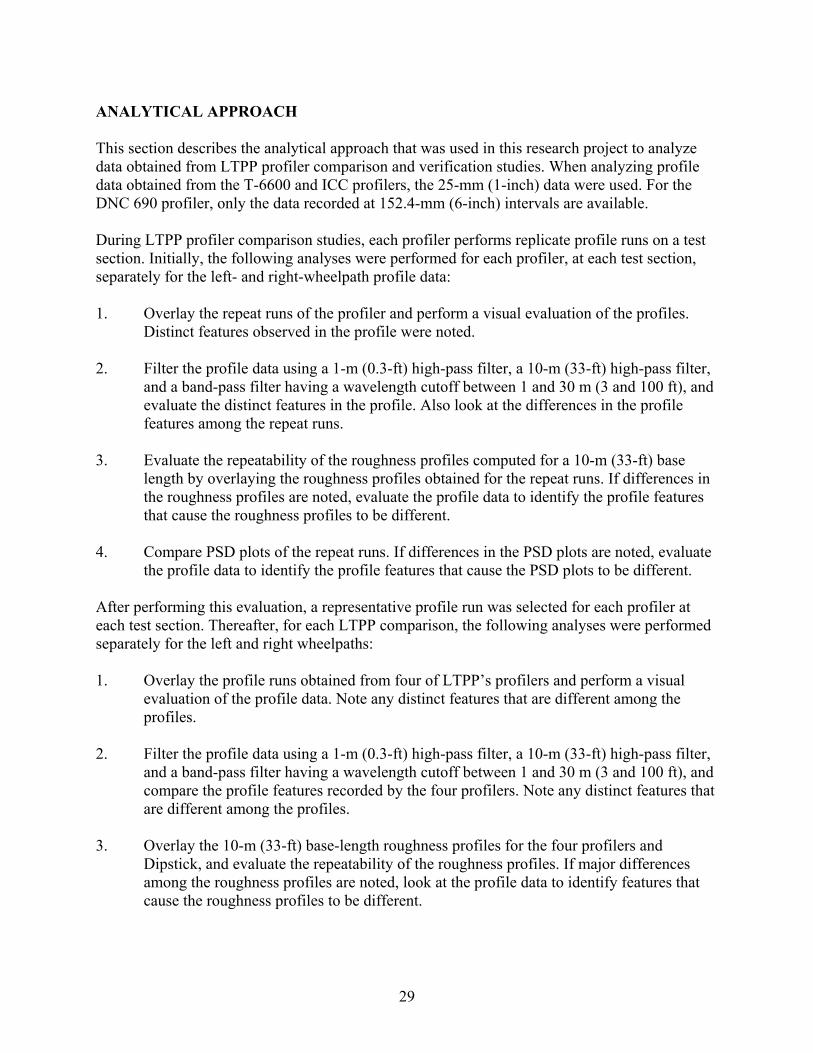
ANALYTICAL APPROACH

cal approach that was used in this research project to analyze ata obtained from LTPP profiler comparison and verification studies. When analyzing profile

n a test ction. Initially, the following analyses were performed for each profiler, at each test section,

a visual evaluation of the profiles. Distinct features observed in the profile were noted.

2. lter, a 10-m (33-ft) high-pass filter, and a band-pass filter having a wavelength cutoff between 1 and 30 m (3 and 100 ft), and

3. roughness profiles computed for a 10-m (33-ft) base

length by overlaying the roughness profiles obtained for the repeat runs. If differences in s

4. ces in the PSD plots are noted, evaluate

the profile data to identify the profile features that cause the PSD plots to be different.

After pach test section. Thereafter, for each LTPP comparison, the following analyses were performed

four of LTPP’s profilers and perform a visual evaluation of the profile data. Note any distinct features that are different among the

2. profile data using a 1-m (0.3-ft) high-pass filter, a 10-m (33-ft) high-pass filter,

and a band-pass filter having a wavelength cutoff between 1 and 30 m (3 and 100 ft), and

3. gth roughness profiles for the four profilers and

Dipstick, and evaluate the repeatability of the roughness profiles. If major differences that

This section describes the analytiddata obtained from the T-6600 and ICC profilers, the 25-mm (1-inch) data were used. For the DNC 690 profiler, only the data recorded at 152.4-mm (6-inch) intervals are available. During LTPP profiler comparison studies, each profiler performs replicate profile runs oseseparately for the left- and right-wheelpath profile data: 1. Overlay the repeat runs of the profiler and perform

Filter the profile data using a 1-m (0.3-ft) high-pass fi

evaluate the distinct features in the profile. Also look at the differences in the profile features among the repeat runs.

Evaluate the repeatability of the

the roughness profiles are noted, evaluate the profile data to identify the profile featurethat cause the roughness profiles to be different.

Compare PSD plots of the repeat runs. If differen

erforming this evaluation, a representative profile run was selected for each profiler at

eseparately for the left and right wheelpaths: 1. Overlay the profile runs obtained from

profiles.

Filter the

compare the profile features recorded by the four profilers. Note any distinct features that are different among the profiles.

Overlay the 10-m (33-ft) base-len

among the roughness profiles are noted, look at the profile data to identify featurescause the roughness profiles to be different.

29

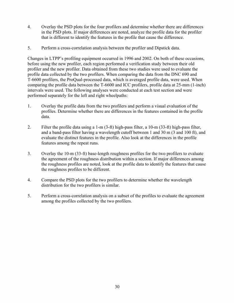
4. Overlay the PSD plots for the four profilers and determine whether there are differences

. Perform a cross-correlation analysis between the profiler and Dipstick data.

hanges in LTPP’s profiling equipment occurred in 1996 and 2002. On both of these occasions,

. Overlay the profile data from the two profilers and perform a visual evaluation of the e

. Filter the profile data using a 1-m (3-ft) high-pass filter, a 10-m (33-ft) high-pass filter,

d

. Overlay the 10-m (33-ft) base-length roughness profiles for the two profilers to evaluate

. Compare the PSD plots for the two profilers to determine whether the wavelength

. Perform a cross-correlation analysis on a subset of the profiles to evaluate the agreement

in the PSD plots. If major differences are noted, analyze the profile data for the profiler that is different to identify the features in the profile that cause the difference.

5 Cbefore using the new profiler, each region performed a verification study between their old profiler and the new profiler. Data obtained from these two studies were used to evaluate the profile data collected by the two profilers. When comparing the data from the DNC 690 and T-6600 profilers, the ProQual-processed data, which is averaged profile data, were used. When comparing the profile data between the T-6600 and ICC profilers, profile data at 25-mm (1-inch)intervals were used. The following analyses were conducted at each test section and were performed separately for the left and right wheelpaths: 1

profiles. Determine whether there are differences in the features contained in the profildata.

2and a band-pass filter having a wavelength cutoff between 1 and 30 m (3 and 100 ft), anevaluate the distinct features in the profile. Also look at the differences in the profile features among the repeat runs.

3the agreement of the roughness distribution within a section. If major differences among the roughness profiles are noted, look at the profile data to identify the features that causethe roughness profiles to be different.

4distribution for the two profilers is similar.

5among the profiles collected by the two profilers.

30

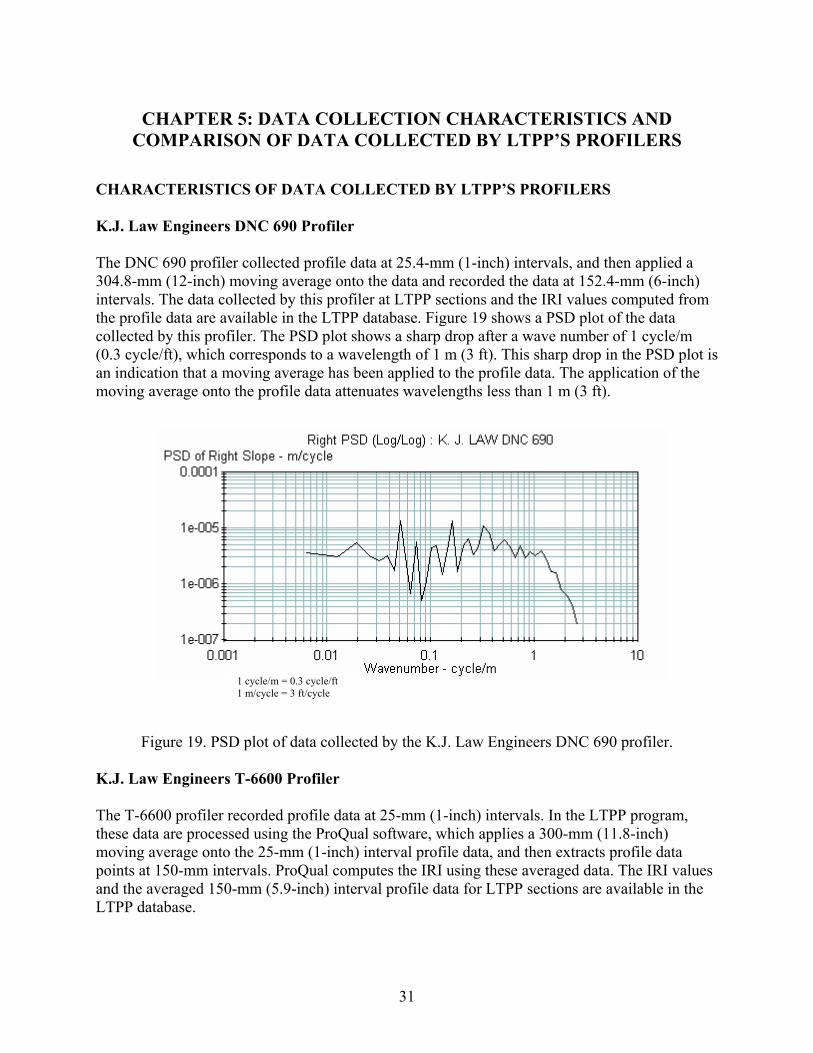
CHAPTER 5: DATA COLLECTION CHARACTERISTICS AND COMPARISON OF DATA COLLECTED BY LTPP’S PROFILERS

CHARACTERISTICS OF DATA COLLECTED BY LTPP’S PROFILERS K.J. Law Engineers DNC 690 Profiler The DNC 690 profiler collected profile data at 25.4-mm (1-inch) intervals, and then applied a 304.8-mm (12-inch) moving average onto the data and recorded the data at 152.4-mm (6-inch) intervals. The data collected by this profiler at LTPP sections and the IRI values computed from the profile data are available in the LTPP database. Figure 19 shows a PSD plot of the data collected by this profiler. The PSD plot shows a sharp drop after a wave number of 1 cycle/m (0.3 cycle/ft), which corresponds to a wavelength of 1 m (3 ft). This sharp drop in the PSD plot is an indication that a moving average has been applied to the profile data. The application of the moving average onto the profile data attenuates wavelengths less than 1 m (3 ft).

1 cycle/m = 0.3 cycle/ft 1 m/cycle = 3 ft/cycle

Figure 19. PSD plot of data collected by the K.J. Law Engineers DNC 690 profiler. K.J. Law Engineers T-6600 Profiler The T-6600 profiler recorded profile data at 25-mm (1-inch) intervals. In the LTPP program, these data are processed using the ProQual software, which applies a 300-mm (11.8-inch) moving average onto the 25-mm (1-inch) interval profile data, and then extracts profile data points at 150-mm intervals. ProQual computes the IRI using these averaged data. The IRI values and the averaged 150-mm (5.9-inch) interval profile data for LTPP sections are available in the LTPP database.

31

Figure 20 shows a PSD plot of the 25-mm (1-inch) data collected by the T-6600 profiler and the PSD plot of the same data after it has been processed using ProQual. Figure 20 shows that there is a significant difference in the profile content between the two profilers for wave numbers greater than 1 cycle/m (0.3 cycle/ft), which corresponds to wavelengths less than 1 m (3 ft). The sharp dropoff seen in the PSD plot for 150-mm (5.9-inch) data for wave numbers greater than 1 cycle/m (0.3 cycle/ft) occurs because the moving average attenuates wavelengths less than 1 m (3 ft) in the profile.

1 cycle/m = 0.3 cycle/ft 1 m/cycle = 3 ft/cycle

Figure 20. PSD plot of data collected by the K.J. Law Engineers T-6600 profiler. International Cybernetics Corporation Profiler The ICC profilers do not record profile data, but rather record the data collected by the height sensors, accelerometers, and the DMI. These data can be used to generate profiles with a 25-mm (1-inch) sampling interval. In the LTPP program, these 25-mm (1-inch) data are processed using the ProQual software, which uses the same procedure as described for the T-6600 profiler. As in the case of the T-6600 profiler, IRI is computed using the averaged data that are at 150-mm (5.9-inch) intervals. The computed IRI values and the averaged profile data for LTPP sections are available in the LTPP database. Figure 21 shows a PSD plot of the 25-mm (1-inch) data collected by the ICC profiler and the PSD plot of the same data after it had been processed using ProQual. The trend between the 25-mm (1-inch) data and the 150-mm (5.9-inch) data seen in this figure is similar to the trend that was observed for the T-6600 profiler, where the application of the moving average caused profile features that have a wave number greater than 1 cycle/m (0.3 cycle/ft) to become attenuated.

32

COMPARISON OF K.J. LAW ENGINEERS DNC 690 AND T-6600 PROFILERS Comparison of Profile Data The DNC 690 profiler recorded profile data at 152.4-mm (6-inch) intervals, while the T-6600 profiler recorded profile data at 25-mm (1-inch) intervals. The DNC 690 and T-6600 profilers applied a 91-m (300-ft) and 100-m (328-ft) upper-wavelength cutoff filter to the profile data, respectively.

1 cycle/m = 0.3 cycle/ft 1 m/cycle = 3 ft/cycle

Figure 21. PSD plot of data collected by the ICC profiler. Figure 22 shows overlaid profile plots of data collected at the same site by the DNC 690 and T-6600 profilers. These data are from the smooth AC section that was used by the North Central region for the 1996 profiler verification test.(24) Figure 23 shows a similar plot at the rough AC section used by the North Central region for the same study.

33

-8-6-4-202468

10

0 20 40 60 80 100 120 140 160

Distance (m)

Elev

atio

n (m

m)

DNC 690

T-6600

2.54 mm = 1 inch 1 m = 3.28 ft

Figure 22. Data collected by the North Central K.J. Law Engineers DNC 690 and T-6600 profilers at the smooth AC site during the 1996 verification test.

-60

-40

-20

0

20

40

60

0 20 40 60 80 100 120 140 160

Distance (m)

Ele

vatio

n (m

m)

DNC 690

T-6600

T-6600 DNC 690

2.54 mm = 1 inch 1 m = 3.28 ft

Figure 23. Data collected by the North Central K.J. Law Engineers DNC 690 and T-6600 profilers at the rough AC site during the 1996 verification test.

The data collected by the two profilers overlay extremely well at the smooth AC section, while at the rough AC section, the agreement is less when compared to the agreement seen at the smooth AC section. At the rough AC section, although there is a slight shift between the two profiles, an evaluation of the profile data using filtering techniques shows that similar profile features are captured by both profilers. The overall shape of a profile plot primarily depends on the long-wavelength content in the profile. There is a slight difference in the long-wavelength cutoff limit used by the two profilers, which can cause some differences to occur in the profile plots. The long-wavelength content at

34

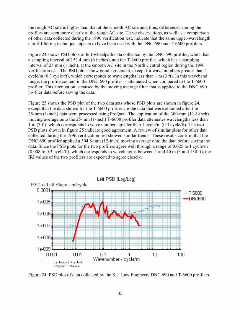
the rough AC site is higher than that at the smooth AC site and, thus, differences among the profiles are seen more clearly at the rough AC site. These observations, as well as a comparison of other data collected during the 1996 verification test, indicate that the same upper-wavelength cutoff filtering technique appears to have been used with the DNC 690 and T-6600 profilers. Figure 24 shows PSD plots of left-wheelpath data collected by the DNC 690 profiler, which has a sampling interval of 152.4 mm (6 inches), and the T-6600 profiler, which has a sampling interval of 25 mm (1 inch), at the smooth AC site in the North Central region during the 1996 verification test. The PSD plots show good agreement, except for wave numbers greater than 1 cycle/m (0.3 cycle/ft), which corresponds to wavelengths less than 1 m (3 ft). In this waveband range, the profile content in the DNC 690 profiler is attenuated when compared to the T-6600 profiler. This attenuation is caused by the moving average filter that is applied to the DNC 690 profiler data before saving the data. Figure 25 shows the PSD plot of the two data sets whose PSD plots are shown in figure 24, except that the data shown for the T-6600 profiler are the data that were obtained after the 25-mm (1-inch) data were processed using ProQual. The application of the 300-mm (11.8-inch) moving average onto the 25-mm (1-inch) T-6600 profiler data attenuates wavelengths less than 1 m (3 ft), which corresponds to wave numbers greater than 1 cycle/m (0.3 cycle/ft). The two PSD plots shown in figure 25 indicate good agreement. A review of similar plots for other data collected during the 1996 verification test showed similar trends. These results confirm that the DNC 690 profiler applied a 304.8-mm (12-inch) moving average onto the data before saving the data. Since the PSD plots for the two profilers agree well through a range of 0.025 to 1 cycle/m (0.008 to 0.3 cycle/ft), which corresponds to wavelengths between 1 and 40 m (3 and 130 ft), the IRI values of the two profilers are expected to agree closely.

1 cycle/m = 0.3 cycle/ft 1 m/cycle = 3 ft/cycle

Figure 24. PSD plot of data collected by the K.J. Law Engineers DNC 690 and T-6600 profilers.

35

Figure 25. PSD plots of K.J. Law Engineers DNC 690 profiler data and ProQual-processed

num

When comparison testing between the two profilers is performed, the profiler driver should do the Align the profiler along the wheelpaths.

1 cycle/m = 0.3 cycle/ft 1 m/cycle = 3 ft/cycle

T-6600 profiler data.

The PSD plots also indicate that the spectral content of the data collected at the same site by the two profilers was similar. This indicates that the profile features that are recorded by the two profilers are similar. (Note: These observations are only valid when the DNC 690 profiler data are compared to ProQual-processed T-6600 profiler data. If 25-mm (1-inch) T-6600 profiler data are compared to DNC 690 profiler data, differences among the profile data will be seen for wave

bers greater than 1 cycle/m (0.3 cycle/ft).) The PSD plots also indicated good agreement between the two profilers for low wave numbers (long wavelengths), which is an indication that the filtering technique used by the two profilers for the upper-wavelength cutoff is similar. The slight differences seen in the PSD plots for the low wave numbers (long wavelengths) are probably related to the different upper-wavelength cutoff values that were used in the two profilers, which are 91 m (300 ft) for the DNC 690 profiler and 100 m (328 ft) for the T-6600 profiler.

Comparison of IRI Values

following two tasks accurately:

•• Maintain a consistent path within the test section. If the profiler driver does not correctly align the profiler along the wheelpaths, the longitudinal path followed by the sensors of the different profilers will be different. This can cause IRI

36

obtained from the different profilers to vary. After aligning the profiler along the wheelpaths, the driver should also follow a consistent path within the test section without lateral wander. If theis variability in the path that is followed within the section, it can result in differences in IRI when the two profilers are being compared. The ability of a driver to correctly align the profiler along the wheelpaths and to follow a consistent path within the section can vary among drivers. Drivers who are more experienced iprofiling c

re

n an probably do these two tasks much better than a driver who is inexperienced in

rofiling. A driver who is experienced in profiling probably will also be able to follow a more g repeat measurements at a site than a person who does not have

uch experience in operating the profiler.

ity within the section during profiling, will sually have a greater impact on the IRI for sections that have distresses. This is because, in such

ment features either to be included or missed in der is an issue that can sometimes

omplicate the analysis when the IRI from different profilers are compared.

is

shown in table 3. As shown in this table, the ercent change in IRI will vary for different pavements. Some pavements showed extremely

hange

Section IRI (m/km) Percent Change in IRI

pconsistent path when obtaininm Not following the correct wheelpath, or variabilusections, lateral variations can cause certain pavethe profile, thus affecting the IRI. The effect of lateral wanc A study performed for an NCHRP project found that variations in the longitudinal path thatfollowed during profiling could have a significant effect on IRI.(1) In this study, the effect of lateral variations in profiling was studied at seven test sections. The percent change in IRI that was obtained for each wheelpath at the test sections for a 0.3-m (1-ft) lateral shift in the longitudinal path to the left and to the right isplarge variations in IRI for a 0.3-m (1-ft) shift from the wheelpath. Generally, the percent cin IRI that was observed along the left wheelpath was less than that obtained for the right wheelpath.

Table 3. Changes in IRI caused by lateral variations in the longitudinal path.

Wheelpath Shifted 0.3 m Right Shifted 0.3 m Left Left Right Wheelpath Wheelpath Left Right Left Right

New AC 0.85 0.98 −4 6 −4 −7 AC with Transverse Cracks 1.20 1.22 −3 34 8 2 Old AC 1.85 2.63 −7 0 −17 −22 1-year-old PCC 0.84 1.41 1 13 −4 −21 3-year-old PCC 0.59 0.58 −5 14 15 7 6-year-old PCC 1.41 1.75 4 13 −4 −3 Severely Faulted PCC 3.67 3.83 −1 1 8 −2

After each r

1 m = 3.28 ft 1 m/km = 5.28 ft/mi

egional contractor accepted delivery of the T-6600 profiler in 1996, they performed a comparison of this profiler and the DNC 690 profiler. Four test sections were used in each region

37

to perform m this test are described in appendix B. In the reports e IRI value for a wheelpath from the that were pe puted u ng different procedures. In this r ct aobtained from all four regions to compare value DNC 690 and T-6600 profilers. The IRI values obtained fo sequen 2 tes ere u this a c ite 1 ern region for the DNC 690 profiler, where sequence 1 values were used because sequence 2 data had s pi he ge IRI for each wheelpath at each test section wa th run had the least standard deviations in IRI for the mean IRI (i.e., the average IRI for ft a ht wheelpaths). The comp veragva ilers for all reg re in t e 4. Whe l 4 regi ere c red, the 16 test sites (3 eelp ons between the 2 profilers co Figure 26 shows the IRI relationship between the two profilers, w e data ob ned for

h wn. There is very good agreement in the IRI values obtained by the two ro one case along the left wheelpath. This data point corresponds to the left

this comparison. (See references 24, 25, 26, and 27.) The results obtained froprepared by th

multiple runse regional contractors, the averagrformed at a site was com

si esearch proje , a consistent method w s used on data the IRI s between the

r ce ting w sed in nalysis (ex ept at s in the West

aturation ss computed using the IRI for

kes). T averae five s that the le nd rig uted a e IRI

lues for both prof ions a shown abl n al ons w onsidere were a total of 2 wh aths) where IRI comparis

uld be made.

her tai 32 w eelpaths are sho

filers, except forpwheelpath of site 2 in the Western region. An evaluation of the data indicated that the data collected by the DNC 690 profiler had a significant number of spikes that were caused by sunlight being picked up by the sensor, which resulted in a high IRI value. The correlation coefficient for the data shown in figure 26 is 0.98.

38

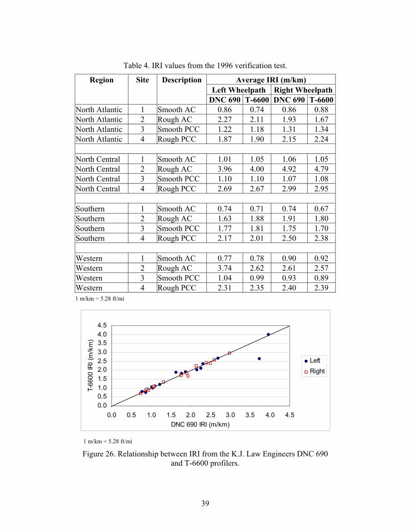
Table 4. IRI values from the 1996 verification test.

Region Site Description Average IRI (m/km) Left Wheelpath Right Wheelpath DNC 690 T-6600 DNC 690 T-6600North Atlantic 1 Smooth AC 0.86 0.74 0.86 0.88 North Atlantic 2 Rough AC 2.27 2.11 1.93 1.67 North Atlantic 3 Smooth PCC 1.22 1.18 1.31 1.34 North Atlantic 4 Rough PCC 1.87 1.90 2.15 2.24 North Central 1 Smooth AC 1.01 1.05 1.06 1.05 North Central 2 Rough AC 3.96 4.00 4.92 4.79 North Central 3 Smooth PCC 1.10 1.10 1.07 1.08 North Central 4 Rough PCC 2.69 2.67 2.99 2.95 Southern 1 Smooth AC 0.74 0.71 0.74 0.67 Southern 2 Rough AC 1.63 1.88 1.91 1.80 Southern 3 Smooth PCC 1.77 1.81 1.75 1.70 Southern 4 Rough PCC 2.17 2.01 2.50 2.38 Western 1 Smooth AC 0.77 0.78 0.90 0.92 Western 2 Rough AC 3.74 2.62 2.61 2.57 Western 3 Smooth PCC 1.04 0.99 0.93 0.89 Western 4 Rough PCC 2.31 2.35 2.40 2.39

0.00.51.01.52.02.53.03.54.04.5

0.0 0.5 1.0 1.5 2.0 2.5 3.0 3.5 4.0 4.5DNC 690 IRI (m/km)

T-66

00 IR

I (m

/km

)

LeftRight

1 m/km = 5.28 ft/mi

1 m/km = 5.28 ft/mi

Figure 26. Relationship between IRI from the K.J. Law Engineers DNC 690 and T-6600 profilers.

39

The difference in IRI between the DNC 690 and T-6600 profilers (DNC 690 IRI – T-6600 IRI) was computed along each wheelpath for all of the test sections. These data are shown in figure 27 as a function of the IRI for the wheelpath, where the IRI for the wheelpath was computed by averaging the IRI obtained for that wheelpath by the DNC 690 and T-6600 profilers. Of the 32 available cases, the difference in IRI was within ±0.10 m/km (±6 inches/mi) for 23 cases. For six cases, the difference was between 0.10 and 0.20 m/km (6 and 13 inches/mi). There was one case where the difference was between −0.20 and −0.30 m/km (−13 and −19 inches/mi), one case where the difference was between 0.20 and 0.30 m/km (13 and 19 inches/mi), and one case where the difference was greater than 1.1 m/km (70 inches/mi) (this data point is not shown in figure 27).

-0.3

-0.2

-0.1

0.0

0.1

0.2

0.3

0.0 1.0 2.0 3.0 4.0 5.0 6.0

IRI of Wheelpath (m/km)

DN

C 6

90 IR

I -T-

6600

IRI (

m/k

m)

LeftRight

-0.3

-0.2

-0.1

0.0

0.1

0.2

0.3

0.0 1.0 2.0 3.0 4.0 5.0 6.0

IRI of Wheelpath (m/km)

DN

C 6

90 IR

I -T-

6600

IRI (

m/k

m)

LeftRight

1 m/km = 5.28 ft/mi

Figure 27. Differences in IRI between the K.J. Law Engineers DNC 690 and T-6600 profilers: All regions.

An investigation was performed separately for each region to identify the cause of the difference in IRI between the two profilers for cases where the difference in IRI was outside ±0.10 m/km (±6 inches/mi). In each region, the difference in IRI between the DNC 690 and T-6600 profilers (DNC 690 IRI – T-6600 IRI) for each wheelpath was plotted as a function of the IRI for the wheelpath, with the IRI for the wheelpath computed by averaging IRI obtained by the two profilers for that wheelpath. North Atlantic Region Figure 28 shows the difference in IRI from the DNC 690 and T-6600 profilers at the test sections tested by the North Atlantic profilers as a function of the IRI for the wheelpath. A difference in IRI between the DNC 690 and T-6600 profilers (DNC 690 –IRI – T-6600 IRI) that was outside ±0.10 m/km (±6 inches/mi) was observed for the following three cases: (1) left wheelpath of site 1 (a difference of 0.12 m/km (8 inches/mi)), (2) left wheelpath of site 2 (a difference of 0.16 m/km (10 inches/mi)), and (3) right wheelpath of site 2 (a difference of 0.26 m/km (16 inches/mi)).

40

Site 1: The left-wheelpath IRI from the DNC 690 profiler was 0.12 m/km (8 inches/mi) higher than IRI obtained by the T-6600 profiler. The DNC 690 profiler conducted six runs on this section. IRI along the left wheelpath for these six runs ranged from 0.83 to 0.87 m/km (53 to 55 inches/mi). The T-6600 profiler conducted nine runs at this site, and the left-wheelpath IRI for eight runs ranged from 0.72 to 0.77 m/km (46 to 49 inches/mi); however, there was one run that had an IRI of 0.85 m/km (54 inches/mi). The roughness profile of this run overlaid extremely well with the roughness profiles obtained by the DNC 690 profiler. This indicates that the probable cause of the difference in IRI between the two profilers was a difference in the paths that were followed during profiling.

North Atlantic

-0.15

-0.10-0.05

0.000.05

0.100.15

0.200.25

0.30

0.0 0.5 1.0 1.5 2.0 2.5

IRI of Wheelpath (m/km)

Left

Right

Site 2

Site 2Site 1

North Atlantic

-0.15

-0.10-0.05

0.000.05

0.100.15

0.200.25

0.30

0.0 0.5 1.0 1.5 2.0 2.5

IRI of Wheelpath (m/km)

Left

Right

Site 2

Site 2Site 1

DN

C IR

I–T-

6600

(m/k

m)

1 m/km = 5.28 ft/mi

Figure 28. Differences in IRI between the K.J. Law Engineers DNC 690 and T-6600 profilers: North Atlantic region.

Site 2: IRI from the DNC 690 profiler was higher than IRI from the T-6600 profiler by 0.16 m/km (10 inches/mi) and 0.26 m/km (16 inches/mi) for the left and right wheelpaths, respectively. This analysis used IRI values obtained during sequence 2 testing. The average IRI from the T-6600 profiler from sequence 1 testing at this site, along the left and right wheelpaths, were 2.21 m/km (140 inches/mi) and 1.89 m/km (120 inches/mi), respectively. These values compare extremely well with the IRI values obtained for the left and right wheelpaths by the DNC 690 profiler (2.27 m/km (144 inches/mi) and 1.93 m/km (122 inches/mi), respectively). This section had significant transverse and longitudinal cracking along both wheelpaths throughout the test section. Thus, the differences in IRI that were observed between the two profilers for sequence 2 testing are attributed to variations in the wheelpaths followed by the two profilers. North Central Region Figure 29 shows the differences in IRI from the DNC 690 and T-6600 profilers at the test sections in the North Central region as a function of the IRI for the wheelpath.

41

A difference in IRI between the DNC 690 and T-6600 profilers that was outside ±0.10 m/km (±6 inches/mi) was observed only along the right wheelpath at site 2, where the IRI from the DNC 690 profiler was higher than that from the T-6000 profiler by 0.13 m/km (8 inches/mi). The right wheelpath at this site is extremely rough. The right-wheelpath IRI for the five selected runs from the DNC 690 profiler ranged from 4.77 to 4.96 m/km (302 to 314 inches/mi), while the IRI for the five selected runs from the T-6600 profiler ranged from 4.74 to 4.81 m/km (301 to 305 inches/mi). These ranges for the two profilers have some overlap. The difference in IRI between the two profilers at this site is attributed to variations in the wheelpaths.

North Central

-0.15-0.10

Figure 29. Differences in IRI between the K.J. Law Engineers DNC 690 and T-6600 profilers: North Central region.

Southern Region Figure 30 shows the difference in IRI from the DNC 690 and T-6600 profilers at the test sections tested by the Southern profilers as a function of the IRI for the wheelpath. Differences in IRI between the DNC 690 and T-6600 profilers (DNC 690 –IRI – T-6600 IRI) that were outside ±0.10 m/km (±6 inches/mi) were observed for the following four cases: (1) left wheelpath of site 2 (a difference of −0.25 m/km (−16 inches/mi)), (2) right wheelpath of site 2 (a difference of 0.11 m/km (10 inches/mi)), (3) left wheelpath of site 4 (a difference of 0.16 m/km (10 inches/mi)), and (4) right wheelpath of site 4 (a difference of 0.12 m/km (7 inches/mi)).

1 m/km = 5.28 ft/mi

-0.050.000.050.100.150.200.250.30

0.0 1.0 2.0 3.0 4.0 5.0 6.0

IRI of Wheelpath (m/km)

LeftRight

Site 2

North Central

-0.15-0.10

0.000.050.100.150.200.250.30

0.0 1.0 2.0 3.0 4.0 5.0 6.0

IRI of Wheelpath (m/km)

-0.05

LeftRight

DN

C IR

I–T-

6600

(m/k

m)

Site 2

42

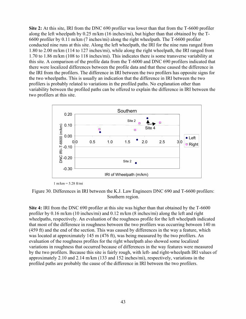
Site 2: At this site, IRI from the DNC 690 profiler was lower than that from the T-6600 profiler along the left wheelpath by 0.25 m/km (16 inches/mi), but higher than that obtained by the T-6600 profiler by 0.11 m/km (7 inches/mi) along the right wheelpath. The T-6600 profiler conducted nine runs at this site. Along the left wheelpath, the IRI for the nine runs ranged from 1.80 to 2.00 m/km (114 to 127 inches/mi), while along the right wheelpath, the IRI ranged from 1.70 to 1.86 m/km (108 to 118 inches/mi). This indicates there is some transverse variability at this site. A comparison of the profile data from the T-6000 and DNC 690 profilers indicated that there were localized differences between the profile data and that these caused the difference in the IRI from the profilers. The difference in IRI between the two profilers has opposite signs for the two wheelpaths. This is usually an indication that the difference in IRI between the two profilers is probably related to variations in the profiled paths. No explanation other than variability between the profiled paths can be offered to explain the difference in IRI between the two profilers at this site.

Southern

-0.30

Figure 30. Differences in IRI between the K.J. Law Engineers DNC 690 and T-6600 profilers: Southern region.

Site 4: IRI from the DNC 690 profiler at this site was higher than that obtained by the T-6600 profiler by 0.16 m/km (10 inches/mi) and 0.12 m/km (8 inches/mi) along the left and right wheelpaths, respectively. An evaluation of the roughness profile for the left wheelpath indicated that most of the difference in roughness between the two profilers was occurring between 140 m (459 ft) and the end of the section. This was caused by differences in the way a feature, which was located at approximately 145 m (476 ft), was being measured by the two profilers. An evaluation of the roughness profiles for the right wheelpath also showed some localized variations in roughness that occurred because of differences in the way features were measured by the two profilers. Because this site is fairly rough, with left- and right-wheelpath IRI values of approximately 2.10 and 2.14 m/km (133 and 152 inches/mi), respectively, variations in the profiled paths are probably the cause of the difference in IRI between the two profilers.

1 m/km = 5.28 ft/mi

-0

-0

.20

.10

0.00

0.10

0.20

0.0 0.5 1.0 1.5 2.0 2.5 3.0

IRI of Wheelpath (m/km)

LeftRight

Site 2

Site 2

Site 4

Southern

-0.30

.20

.10

0.00

0.10

0.20

0.0 0.5 1.0 1.5 2.0 2.5 3.0

IRI of Wheelpath (m/km)

-0

-0

LeftRight

Site 2

Site 2

Site 4

DN

C IR

I–T-

6600

(m/k

m)

43

Western Region Figure 31 shows the difference in IRI from the DNC 690 and T-6600 profilers at the sections tested by the two Western profilers as a function of the IRI for the wheelpath. The difference in IRI between the two profilers was within ±0.10 m/km (±6 inches/mi) for all of the cases except one. This case was along the left wheelpath at section 2, where the difference in IRI was 1.1 m/km (70 inches/mi). This occurred because data collected by the DNC 690 profiler was contaminated by saturation spikes. This data point is not shown in figure 31. Cross Correlation of IRI The cross-correlation technique provides a method to compare the magnitude and the spatial distribution of IRI between two devices. This technique was used to compare IRI obtained by the DNC 690 and T-6600 profilers using data obtained during the 1996 verification testing in the North Central and Western regions. When using the cross-correlation technique, the DNC 690 profiler was considered to be the “correct” device and, thus, the analysis will indicate how well the T-6600 profiler reproduced the results from the DNC 690 profiler.

Western

-0.15-0.10-0.050.000.050.100.150.200.250.30

0.0 1.0 2.0 3.0

IRI of Wheelpath (m/km)

LeftRight

Western

-0.15-0.10-0.050.000.050.100.150.200.250.30

0.0 1.0 2.0 3.0

IRI of Wheelpath (m/km)

LeftRight

DN

C IR

I–T-

6600

(m/k

m)

1 m/km = 5.28 ft/mi

Figure 31. Differences in IRI between the K.J. Law Engineers DNC 690 and T-6600 profilers: Western region.

One representative run was selected for each profiler at each site to perform this analysis. In this analysis, for the T-6600 profiler, the ProQual-processed averaged data that are at 150-mm (5.9-inch) intervals was used, while for the DNC 690 profiler, the 152.4-mm (6-inch) data obtained by the profiler was used. Because the data collected by the DNC 690 profiler is considered to be the correct data, any deviations in the path followed by the T-6600 profiler from the path followed by the DNC 690 profiler will affect the results. The results of the cross-correlation analysis are presented in table 5.

44

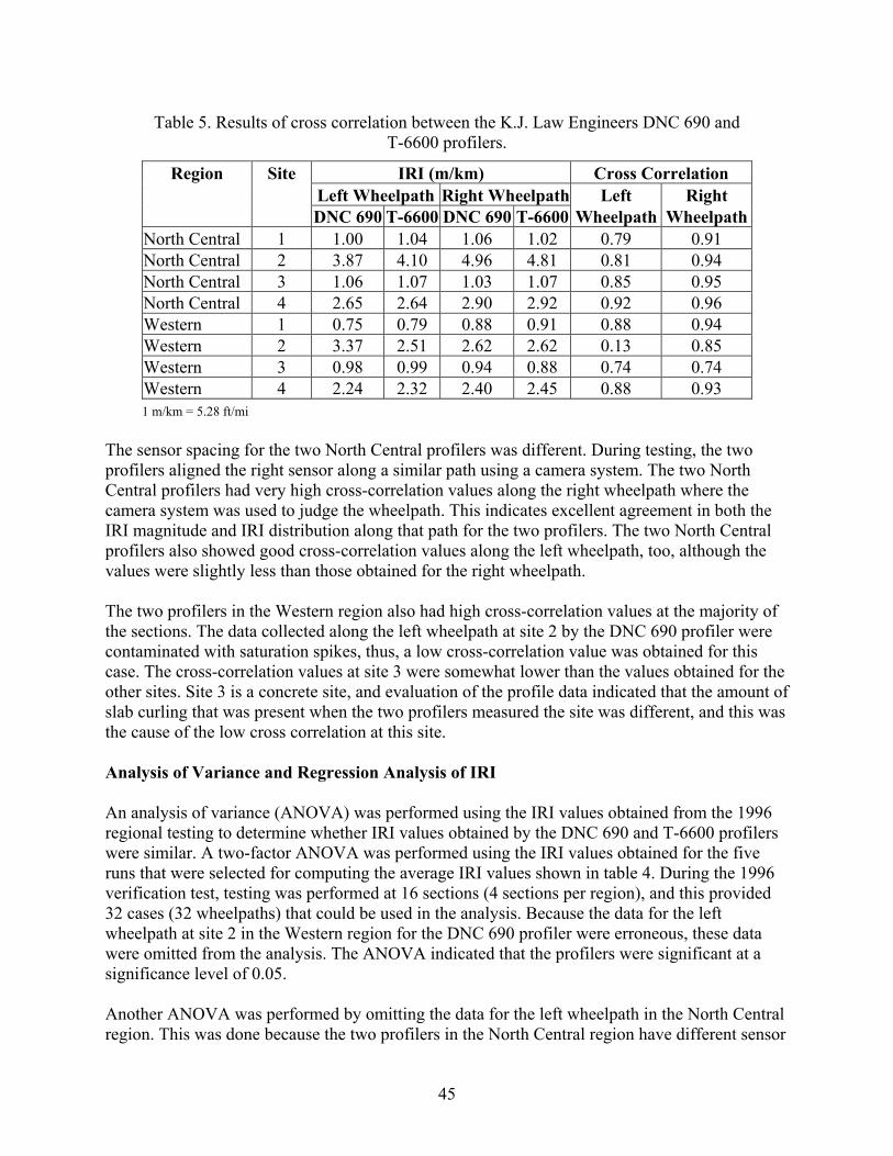
Table 5. Results of cross correlation between the K.J. Law Engineers DNC 690 and

T-6600 profilers.

Region Site IRI (m/km) Cross Correlation Left Wheelpath Right Wheelpath Left Right DNC 690 T-6600 DNC 690 T-6600 Wheelpath WheelpathNorth Central 1 1.00 1.04 1.06 1.02 0.79 0.91 North Central 2 3.87 4.10 4.96 4.81 0.81 0.94 North Central 3 1.06 1.07 1.03 1.07 0.85 0.95 North Central 4 2.65 2.64 2.90 2.92 0.92 0.96 Western 1 0.75 0.79 0.88 0.91 0.88 0.94 Western 2 3.37 2.51 2.62 2.62 0.13 0.85 Western 3 0.98 0.99 0.94 0.88 0.74 0.74 Western 4 2.24 2.32 2.40 2.45 0.88 0.93

1 m/km = 5.28 ft/mi The sensor spacing for the two North Central profilers was different. During testing, the two profilers aligned the right sensor along a similar path using a camera system. The two North Central profilers had very high cross-correlation values along the right wheelpath where the camera system was used to judge the wheelpath. This indicates excellent agreement in both the IRI magnitude and IRI distribution along that path for the two profilers. The two North Central profilers also showed good cross-correlation values along the left wheelpath, too, although the values were slightly less than those obtained for the right wheelpath. The two profilers in the Western region also had high cross-correlation values at the majority of the sections. The data collected along the left wheelpath at site 2 by the DNC 690 profiler were contaminated with saturation spikes, thus, a low cross-correlation value was obtained for this case. The cross-correlation values at site 3 were somewhat lower than the values obtained for the other sites. Site 3 is a concrete site, and evaluation of the profile data indicated that the amount of slab curling that was present when the two profilers measured the site was different, and this was the cause of the low cross correlation at this site. Analysis of Variance and Regression Analysis of IRI An analysis of variance (ANOVA) was performed using the IRI values obtained from the 1996 regional testing to determine whether IRI values obtained by the DNC 690 and T-6600 profilers were similar. A two-factor ANOVA was performed using the IRI values obtained for the five runs that were selected for computing the average IRI values shown in table 4. During the 1996 verification test, testing was performed at 16 sections (4 sections per region), and this provided 32 cases (32 wheelpaths) that could be used in the analysis. Because the data for the left wheelpath at site 2 in the Western region for the DNC 690 profiler were erroneous, these data were omitted from the analysis. The ANOVA indicated that the profilers were significant at a significance level of 0.05. Another ANOVA was performed by omitting the data for the left wheelpath in the North Central region. This was done because the two profilers in the North Central region have different sensor

45

spacing, and they were aligned along the right wheelpath during testing. This analysis also found that the profilers were significant at a significance level of 0.05. Thereafter, separate ANOVAs were performed for each region. The only case where the profilers were not significant was in the Western region. Thereafter, for each region, separate ANOVAs were performed for each wheelpath. The only cases where the profilers were not significant at a significance level of 0.05 were for the left and right wheelpaths in the Western region, and for the left wheelpath in the North Central region. A regression analysis was performed for the IRI from the DNC 690 and T-6600 profilers. The IRI for the five runs that were selected at each section to compute the average IRI value in the previous analysis were used in the regression. This provided 155 pairs of data for the regression (i.e., four regions x four sections per region x two wheelpaths per section x five runs per section, less the erroneous left-wheelpath runs at section 2 in the Western region). The following relationship was obtained from the regression:

(1) IRI (T-6600) = 0.982 IRI (DNC 690) + 0.004where:

• IRI (T-6600) = IRI from T-6600 profiler for a wheelpath (m/km). • IRI (DNC 690) = IRI from DNC 690 profiler for a wheelpath (m/km). • R2 = 0.99, standard error = 0.09 m/km.

The regression analysis indicated that IRI from the two profilers were extremely similar; however, IRI obtained from the DNC 690 profiler was predicted to be slightly higher than that obtained from the T-6600 profiler. COMPARISON OF K.J. LAW ENGINEERS T-6600 AND ICC PROFILERS Comparison of Profile Data The data obtained from the 2002 verification test were used for this analysis. Both profilers applied a 100-m (328-ft) upper-wavelength cutoff filter onto the data. The data collected by both profilers along each wheelpath at each site were overlaid to evaluate differences in the data. At some sites, the profiles overlaid extremely well; however, at many sites, there were significant differences among the profiles. Figure 32 shows an example of a case where close agreement was obtained between the profile data from the two profilers. Figure 33 shows an example of a case where there were significant differences between the profile plots. The data shown in figures 32 and 33 are the 25-mm (1-inch) left-wheelpath data collected by the two Western profilers during the 2002 verification test at LTPP sites 320209 and 069107, respectively.

46

-10-8-6-4-202468

0 20 40 60 80 100 120 140Distance (m)

Ele

vatio

n (m

m)

Law

ICC

25.4 mm = 1 inch 1 m = 3.28 ft

Figure 32. Comparison of ICC and K.J. Law Engineers profiles: Western site 320209. An evaluation of all data collected for the 2002 verification test indicated that the profile plots from the two profilers usually overlaid well at sites that did not have much long-wavelength content. However, differences between the profile plots were noticeable at sites that had more long-wavelength content. An evaluation of the profile data using filtering techniques indicated that profile features that were present on the pavement were being measured similarly by both profilers. These observations indicate that there are differences in the long-wavelength data collected by the two profilers. The differences in the long wavelengths appear to be occurring for wavelengths greater than approximately 40 m (131 ft).

47

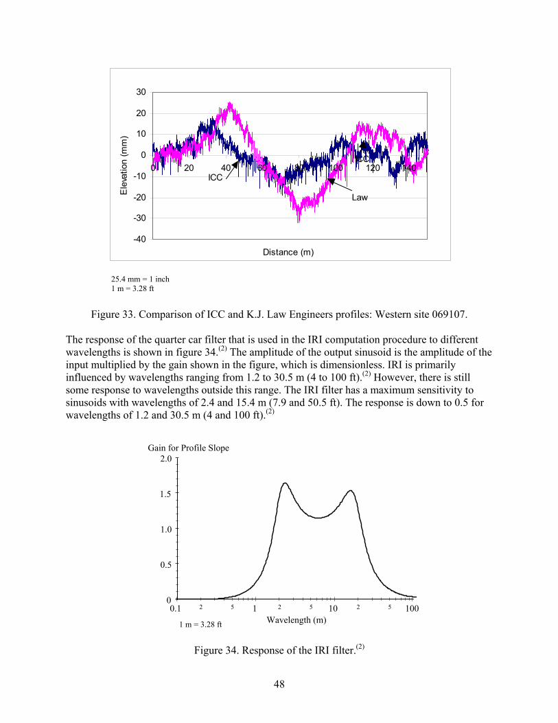
-40

-30

-20

-10

0

10

20

30

0 20 40 60 80 100 120 140

Distance (m)

Ele

vatio

n (m

m)

Law

ICC

ICC

Figure 33. Comparison of ICC and K.J. Law Engineers profiles: Western site 069107. The response of the quarter car filter that is used in the IRI computation procedure to different wavelengths is shown in figure 34.(2) The amplitude of the output sinusoid is the amplitude of the input multiplied by the gain shown in the figure, which is dimensionless. IRI is primarily influenced by wavelengths ranging from 1.2 to 30.5 m (4 to 100 ft).(2) However, there is still some response to wavelengths outside this range. The IRI filter has a maximum sensitivity to sinusoids with wavelengths of 2.4 and 15.4 m (7.9 and 50.5 ft). The response is down to 0.5 for wavelengths of 1.2 and 30.5 m (4 and 100 ft).(2)

0

0.5

1.0

1.5

2.0Gain for Profile Slope

1001010.1 2 5 2 5 2 5

Wavelength (m)

25.4 mm = 1 inch 1 m = 3.28 ft

1 m = 3.28 ft

Figure 34. Response of the IRI filter.(2)

48

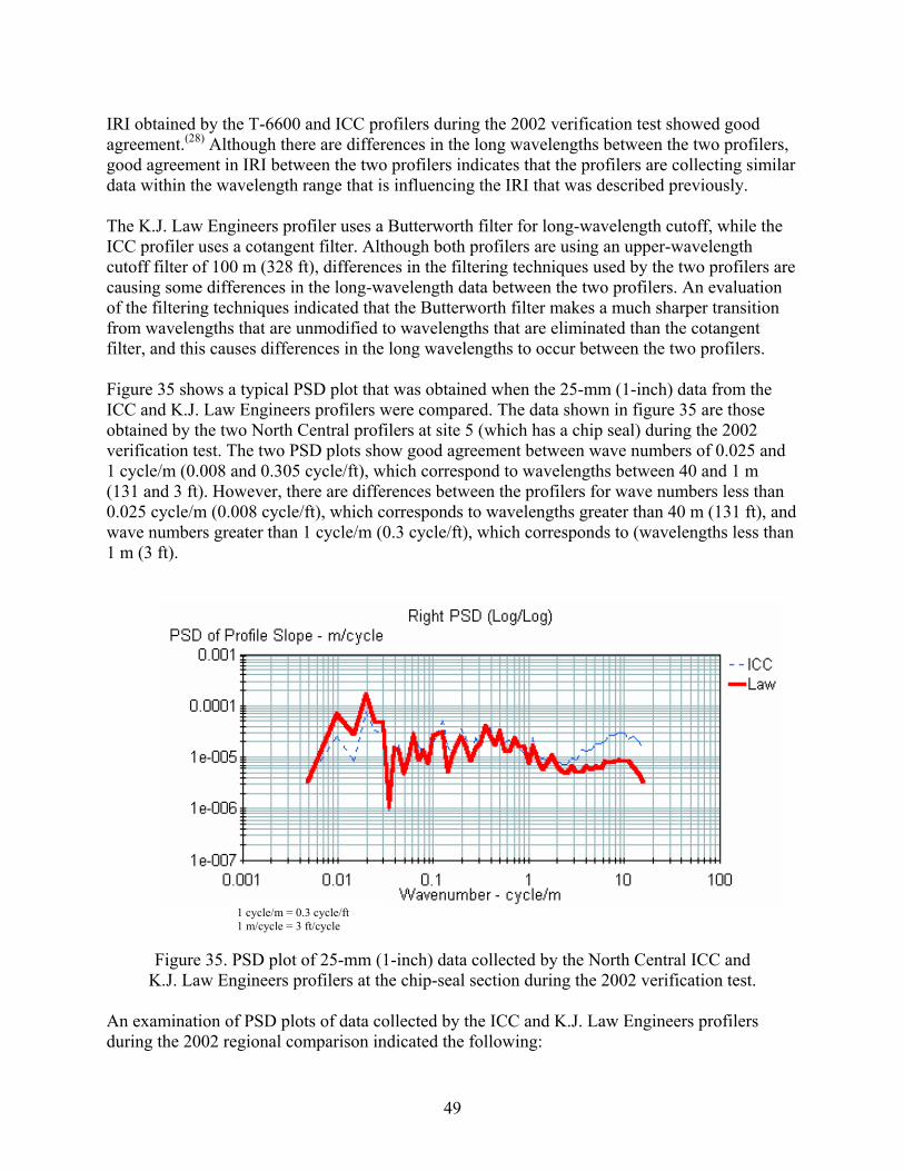
IRI obtained by the T-6600 and ICC profilers during the 2002 verification test showed good agreement.(28) Although there are differences in the long wavelengths between the two profilers, good agreement in IRI between the two profilers indicates that the profilers are collecting similar data within the wavelength range that is influencing the IRI that was described previously. The K.J. Law Engineers profiler uses a Butterworth filter for long-wavelength cutoff, while the ICC profiler uses a cotangent filter. Although both profilers are using an upper-wavelength cutoff filter of 100 m (328 ft), differences in the filtering techniques used by the two profilers are causing some differences in the long-wavelength data between the two profilers. An evaluation of the filtering techniques indicated that the Butterworth filter makes a much sharper transition from wavelengths that are unmodified to wavelengths that are eliminated than the cotangent filter, and this causes differences in the long wavelengths to occur between the two profilers. Figure 35 shows a typical PSD plot that was obtained when the 25-mm (1-inch) data from the ICC and K.J. Law Engineers profilers were compared. The data shown in figure 35 are those obtained by the two North Central profilers at site 5 (which has a chip seal) during the 2002 verification test. The two PSD plots show good agreement between wave numbers of 0.025 and 1 cycle/m (0.008 and 0.305 cycle/ft), which correspond to wavelengths between 40 and 1 m (131 and 3 ft). However, there are differences between the profilers for wave numbers less than 0.025 cycle/m (0.008 cycle/ft), which corresponds to wavelengths greater than 40 m (131 ft), and wave numbers greater than 1 cycle/m (0.3 cycle/ft), which corresponds to (wavelengths less than 1 m (3 ft).

1 cycle/m = 0.3 cycle/ft 1 m/cycle = 3 ft/cycle

Figure 35. PSD plot of 25-mm (1-inch) data collected by the North Central ICC and K.J. Law Engineers profilers at the chip-seal section during the 2002 verification test.

An examination of PSD plots of data collected by the ICC and K.J. Law Engineers profilers during the 2002 regional comparison indicated the following:

49

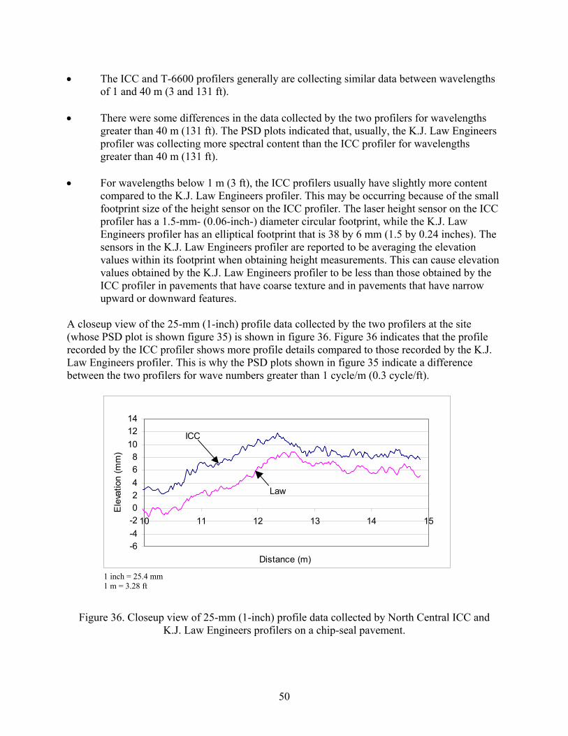
• The ICC and T-6600 profilers generally are collecting similar data between wavelengths

of 1 and 40 m (3 and 131 ft). • There were some differences in the data collected by the two profilers for wavelengths

greater than 40 m (131 ft). The PSD plots indicated that, usually, the K.J. Law Engineers profiler was collecting more spectral content than the ICC profiler for wavelengths greater than 40 m (131 ft).

• For wavelengths below 1 m (3 ft), the ICC profilers usually have slightly more content

compared to the K.J. Law Engineers profiler. This may be occurring because of the small footprint size of the height sensor on the ICC profiler. The laser height sensor on the ICC profiler has a 1.5-mm- (0.06-inch-) diameter circular footprint, while the K.J. Law Engineers profiler has an elliptical footprint that is 38 by 6 mm (1.5 by 0.24 inches). The sensors in the K.J. Law Engineers profiler are reported to be averaging the elevation values within its footprint when obtaining height measurements. This can cause elevation values obtained by the K.J. Law Engineers profiler to be less than those obtained by the ICC profiler in pavements that have coarse texture and in pavements that have narrow upward or downward features.

A closeup view of the 25-mm (1-inch) profile data collected by the two profilers at the site (whose PSD plot is shown figure 35) is shown in figure 36. Figure 36 indicates that the profile recorded by the ICC profiler shows more profile details compared to those recorded by the K.J. Law Engineers profiler. This is why the PSD plots shown in figure 35 indicate a difference between the two profilers for wave numbers greater than 1 cycle/m (0.3 cycle/ft).

-6-4-202468

101214

10 11 12 13 14 15

Distance (m)

Ele

vatio

n (m

m)

ICC

Law

1 inch = 25.4 mm 1 m = 3.28 ft

Figure 36. Closeup view of 25-mm (1-inch) profile data collected by North Central ICC and K.J. Law Engineers profilers on a chip-seal pavement.

50

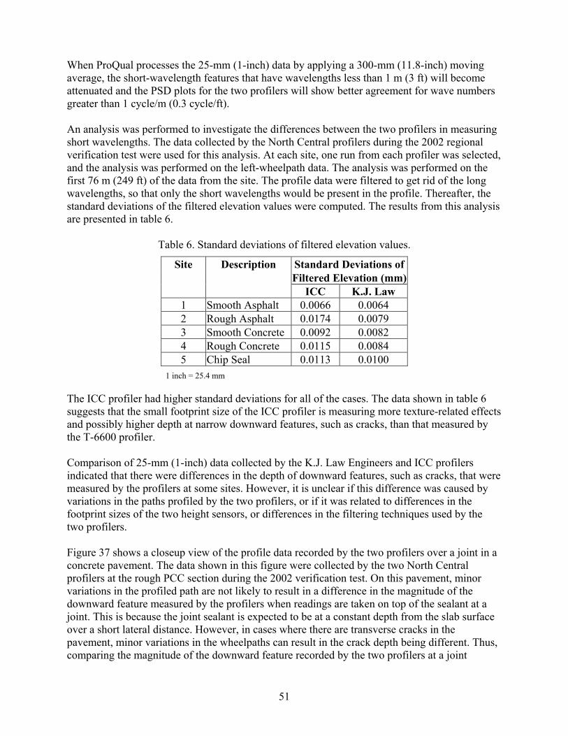
When ProQual processes the 25-mm (1-inch) data by applying a 300-mm (11.8-inch) moving average, the short-wavelength features that have wavelengths less than 1 m (3 ft) will become attenuated and the PSD plots for the two profilers will show better agreement for wave numbers greater than 1 cycle/m (0.3 cycle/ft). An analysis was performed to investigate the differences between the two profilers in measuring short wavelengths. The data collected by the North Central profilers during the 2002 regional verification test were used for this analysis. At each site, one run from each profiler was selected, and the analysis was performed on the left-wheelpath data. The analysis was performed on the first 76 m (249 ft) of the data from the site. The profile data were filtered to get rid of the long wavelengths, so that only the short wavelengths would be present in the profile. Thereafter, the standard deviations of the filtered elevation values were computed. The results from this analysis are presented in table 6.

Table 6. Standard deviations of filtered elevation values.

Site Description Standard Deviations of Filtered Elevation (mm) ICC K.J. Law 1 Smooth Asphalt 0.0066 0.0064 2 Rough Asphalt 0.0174 0.0079 3 Smooth Concrete 0.0092 0.0082 4 Rough Concrete 0.0115 0.0084 5 Chip Seal 0.0113 0.0100

1 inch = 25.4 mm The ICC profiler had higher standard deviations for all of the cases. The data shown in table 6 suggests that the small footprint size of the ICC profiler is measuring more texture-related effects and possibly higher depth at narrow downward features, such as cracks, than that measured by the T-6600 profiler. Comparison of 25-mm (1-inch) data collected by the K.J. Law Engineers and ICC profilers indicated that there were differences in the depth of downward features, such as cracks, that were measured by the profilers at some sites. However, it is unclear if this difference was caused by variations in the paths profiled by the two profilers, or if it was related to differences in the footprint sizes of the two height sensors, or differences in the filtering techniques used by the two profilers. Figure 37 shows a closeup view of the profile data recorded by the two profilers over a joint in a concrete pavement. The data shown in this figure were collected by the two North Central profilers at the rough PCC section during the 2002 verification test. On this pavement, minor variations in the profiled path are not likely to result in a difference in the magnitude of the downward feature measured by the profilers when readings are taken on top of the sealant at a joint. This is because the joint sealant is expected to be at a constant depth from the slab surface over a short lateral distance. However, in cases where there are transverse cracks in the pavement, minor variations in the wheelpaths can result in the crack depth being different. Thus, comparing the magnitude of the downward feature recorded by the two profilers at a joint

51

provides a better choice for comparing the two profilers. The two plots in figure 37 show that the depths of the joint as recorded by the two profilers are very similar; however, the depth recorded by the ICC profiler is slightly higher.

-12-10-8-6-4-20246

61.3 61.5 61.7 61.9 62.1 62.3

Distance (m)

Ele

vatio

n (m

m)

ICCLaw

25.4 mm = 1 inch

1 m = 3.28 ft

Figure 37. Readings taken over a joint by the two profilers. Figure 38 shows the 25-mm (1-inch) profile data collected by the two profilers at this site after the data have been subjected to a 3-m (10-ft) high-pass filter. The slab length in this concrete pavement is 13 m (43 ft). Figure 38 shows that both profile plots are showing all joint locations, and the depths recorded over the joints by the two profilers are very similar.

3-m High Pass Filtered (Profiles Offset)

-10

-5

0

5

10

15

0 25 50 75 100 125 150

Distance (m)

Elev

atio

n (m

m)

Law

ICC

25.4 mm = 1 inch 1 m = 3.28 ft

Figure 38. Profile data obtained by the ICC and K.J. Law Engineers profilers at a concrete site.

52

Although the profilers output data at 25-mm (1-inch) intervals, the height sensors in the profilers are obtaining data at much closer intervals, and are then averaging the data and using the averaged height-sensor value for computing the profile data at 25-mm (1-inch) intervals. If the profilers were just getting height-sensor data at 25-mm (1-inch) intervals, there is always the possibility that a reading may not be obtained on top of a joint. However, because the height sensors are obtaining readings at much closer intervals than 25 mm (1 inch), a reading is always obtained on top of the joint sealant. When the height-sensor data are averaged to obtain a reading every 25 mm (1 inch), the reading obtained over the joint was of sufficient magnitude for the joint to be clearly seen in the filtered profile. Another interesting observation seen in figure 37 is that the profile data show the joint to be a feature that is spread over a distance of 75 mm (3 inches), when the actual width of the joint is on the order of 10 mm (0.4 inches). The joint appears like this in the profile data because of the averaging procedure that is used on the height-sensor data and possibly because of the application of an anti-aliasing filter onto the profile data. The averaging procedure and the anti-aliasing filter will also cause some attenuation in the magnitude of the depth of narrow downward features such as joints and cracks. Comparison of IRI Values An analysis of the IRI values obtained from the 2002 verification test was performed to compare IRI values obtained by the two profilers.(28) In the North Central region, testing by both profilers was performed on the same day. In the North Atlantic region, testing at six of the eight sites was performed on the same day by the two profilers, while in the Western region, a similar procedure was followed for three of the five sites. In the Southern region, testing at the sites by the ICC profiler was performed approximately 1.5 months after testing by the K.J. Law Engineers profiler. The IRI values obtained from the testing (average IRI from five runs) and the test dates are presented in appendix B. There were 23 test sites (46 wheelpaths) where IRI comparisons of the two profilers could be made. Figure 39 shows the IRI relationship between the two profilers, where data for 46 wheelpaths are shown. There is very good agreement in IRI between the two profilers, with the correlation coefficient for the two sets of IRI values being 0.99.

53

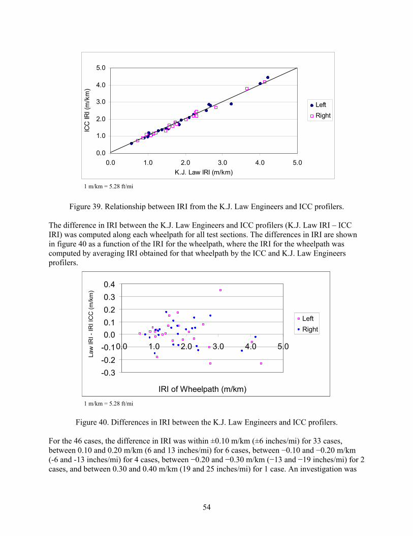
0.0

1.0

2.0

3.0

4.0

5.0

0.0 1.0 2.0 3.0 4.0 5.0K.J. Law IRI (m/km)

ICC

IRI (

m/k

m)

LeftRight

Figure 39. Relationship between IRI from the K.J. Law Engineers and ICC profilers.

The difference in IRI between the K.J. Law Engineers and ICC profilers (K.J. Law IRI – ICC IRI) was computed along each wheelpath for all test sections. The differences in IRI are shown in figure 40 as a function of the IRI for the wheelpath, where the IRI for the wheelpath was computed by averaging IRI obtained for that wheelpath by the ICC and K.J. Law Engineers profilers.

1 m/km = 5.28 ft/mi

1 m/km = 5.28 ft/mi

-0.3-0.2-0.10.00.10.20.30.4

0.0 1.0 2.0 3.0 4.0 5.0

IRI of Wheelpath (m/km)

Law

IRI -

IRI I

CC

(m/k

m)

LeftRight

-0.3-0.2-0.10.00.10.20.30.4

0.0 1.0 2.0 3.0 4.0 5.0

IRI of Wheelpath (m/km)

Law

IRI -

IRI I

CC

(m/k

m)

LeftRight

Figure 40. Differences in IRI between the K.J. Law Engineers and ICC profilers.

For the 46 cases, the difference in IRI was within ±0.10 m/km (±6 inches/mi) for 33 cases, between 0.10 and 0.20 m/km (6 and 13 inches/mi) for 6 cases, between −0.10 and −0.20 m/km (-6 and -13 inches/mi) for 4 cases, between −0.20 and −0.30 m/km (−13 and −19 inches/mi) for 2 cases, and between 0.30 and 0.40 m/km (19 and 25 inches/mi) for 1 case. An investigation was

54

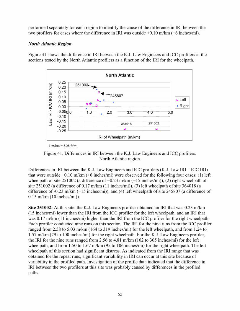
performed separately for each region to identify the cause of the difference in IRI between the two profilers for cases where the difference in IRI was outside ±0.10 m/km (±6 inches/mi). North Atlantic Region Figure 41 shows the difference in IRI between the K.J. Law Engineers and ICC profilers at the sections tested by the North Atlantic profilers as a function of the IRI for the wheelpath.

North Atlantic

-0.25-0.20-0.15-0.10-0.050.000.050.100.150.200.25

0.0 1.0 2.0 3.0 4.0 5.0

IRI of Wheelpath (m/km)

Law

IRI -

ICC

IRI (

m/k

m)

LeftRight

251002364018

251002

245807

North Atlantic

-0.25-0.20-0.15-0.10-0.050.000.050.100.150.200.25

0.0 1.0 2.0 3.0 4.0 5.0

IRI of Wheelpath (m/km)

Law

IRI -

ICC

IRI (

m/k

m)

LeftRight

251002364018

251002

245807

1 m/km = 5.28 ft/mi

Figure 41. Differences in IRI between the K.J. Law Engineers and ICC profilers: North Atlantic region.

Differences in IRI between the K.J. Law Engineers and ICC profilers (K.J. Law IRI – ICC IRI) that were outside ±0.10 m/km (±6 inches/mi) were observed for the following four cases: (1) left wheelpath of site 251002 (a difference of −0.23 m/km (−15 inches/mi)), (2) right wheelpath of site 251002 (a difference of 0.17 m/km (11 inches/mi)), (3) left wheelpath of site 364018 (a difference of -0.23 m/km (−15 inches/mi)), and (4) left wheelpath of site 245807 (a difference of 0.15 m/km (10 inches/mi)). Site 251002: At this site, the K.J. Law Engineers profiler obtained an IRI that was 0.23 m/km (15 inches/mi) lower than the IRI from the ICC profiler for the left wheelpath, and an IRI that was 0.17 m/km (11 inches/mi) higher than the IRI from the ICC profiler for the right wheelpath. Each profiler conducted nine runs on this section. The IRI for the nine runs from the ICC profiler ranged from 2.58 to 5.03 m/km (164 to 319 inches/mi) for the left wheelpath, and from 1.24 to 1.57 m/km (79 to 100 inches/mi) for the right wheelpath. For the K.J. Law Engineers profiler, the IRI for the nine runs ranged from 2.56 to 4.81 m/km (162 to 305 inches/mi) for the left wheelpath, and from 1.50 to 1.67 m/km (95 to 106 inches/mi) for the right wheelpath. The left wheelpath of this section had significant distress. As indicated from the IRI range that was obtained for the repeat runs, significant variability in IRI can occur at this site because of variability in the profiled path. Investigation of the profile data indicated that the difference in IRI between the two profilers at this site was probably caused by differences in the profiled paths.

55

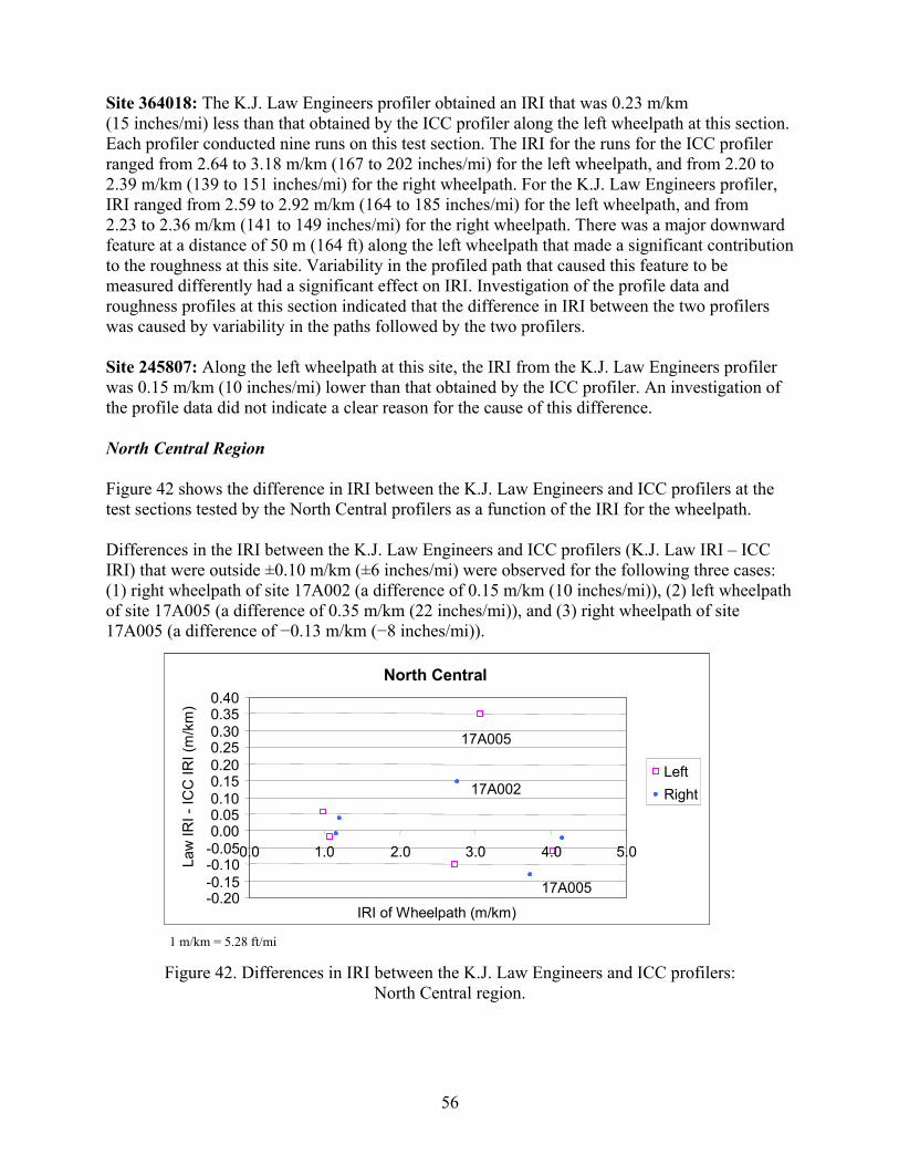
Site 364018: The K.J. Law Engineers profiler obtained an IRI that was 0.23 m/km (15 inches/mi) less than that obtained by the ICC profiler along the left wheelpath at this section. Each profiler conducted nine runs on this test section. The IRI for the runs for the ICC profiler ranged from 2.64 to 3.18 m/km (167 to 202 inches/mi) for the left wheelpath, and from 2.20 to 2.39 m/km (139 to 151 inches/mi) for the right wheelpath. For the K.J. Law Engineers profiler, IRI ranged from 2.59 to 2.92 m/km (164 to 185 inches/mi) for the left wheelpath, and from 2.23 to 2.36 m/km (141 to 149 inches/mi) for the right wheelpath. There was a major downward feature at a distance of 50 m (164 ft) along the left wheelpath that made a significant contribution to the roughness at this site. Variability in the profiled path that caused this feature to be measured differently had a significant effect on IRI. Investigation of the profile data and roughness profiles at this section indicated that the difference in IRI between the two profilers was caused by variability in the paths followed by the two profilers. Site 245807: Along the left wheelpath at this site, the IRI from the K.J. Law Engineers profiler was 0.15 m/km (10 inches/mi) lower than that obtained by the ICC profiler. An investigation of the profile data did not indicate a clear reason for the cause of this difference. North Central Region Figure 42 shows the difference in IRI between the K.J. Law Engineers and ICC profilers at the test sections tested by the North Central profilers as a function of the IRI for the wheelpath. Differences in the IRI between the K.J. Law Engineers and ICC profilers (K.J. Law IRI – ICC IRI) that were outside ±0.10 m/km (±6 inches/mi) were observed for the following three cases: (1) right wheelpath of site 17A002 (a difference of 0.15 m/km (10 inches/mi)), (2) left wheelpath of site 17A005 (a difference of 0.35 m/km (22 inches/mi)), and (3) right wheelpath of site 17A005 (a difference of −0.13 m/km (−8 inches/mi)).

North Central

-0.20-0.15-0.10-0.050.000.050.100.150.200.250.300.350.40

0.0 1.0 2.0 3.0 4.0 5.0

IRI of Wheelpath (m/km)

Law

IRI -

ICC

IRI (

m/k

m)

LeftRight

17A005

17A005

17A002

North Central

-0.20-0.15-0.10-0.050.000.050.100.150.200.250.300.350.40

0.0 1.0 2.0 3.0 4.0 5.0

IRI of Wheelpath (m/km)

Law

IRI -

ICC

IRI (

m/k

m)

LeftRight

17A005

17A005

17A002

1 m/km = 5.28 ft/mi

Figure 42. Differences in IRI between the K.J. Law Engineers and ICC profilers: North Central region.

56

Site 17A002: The IRI from the K.J. Law Engineers profiler was higher than that of the ICC profiler by 0.15 m/km (10 inches/mi) along the right wheelpath at this site. However, along the left wheelpath, the IRI from the K.J. Law Engineers profiler was 0.10 m/km (6 inches/mi) lower than that obtained by the ICC profiler. An investigation of the profile data did not indicate a definitive cause for the difference in IRI between the profilers. However, variability in the wheelpath is a likely cause for the difference in IRI. In this case, the difference in IRI between the K.J. Law Engineers and ICC profilers had opposite signs for the wheelpaths (negative for the left wheelpath and positive for the right wheelpath). This is an indication that the two profilers followed different wheelpaths. Site 17A005: The IRI from the K.J. Law Engineers profiler was higher than that obtained by the ICC profiler by 0.35 m/km (22 inches/mi) along the left wheelpath; along the right wheelpath, the IRI from the K.J. Law Engineers profiler was lower than that obtained by the ICC profiler by 0.13 m/km (8 inches/mi). An investigation of the profile data did not indicate a definitive cause for the difference in IRI between the profilers. Since there was a reversal in signs for the difference in IRI for the two wheelpaths as in the previous case, the differences in IRI between the two profilers at this site were probably cased by variability in the paths followed by the two profilers. Southern Region Figure 43 shows the difference in IRI between the K.J. Law Engineers and ICC profilers at the sections tested by the Southern profilers as a function of the IRI for the wheelpath. Differences in the IRI between the K.J. Law Engineers and ICC profilers (K.J. Law IRI – ICC IRI) that were outside ±0.10 m/km (±6 inches/mi) were observed for the following three cases: (1) left wheelpath of site 48B350 (a difference of 0.17 m/km (11 inches/mi)), (2) right wheelpath of site 48B350 (a difference of −0.13 m/km (−8 inches/mi)), and (3) right wheelpath of site 485253 (a difference of 0.11 m/km (7 inches/mi)). The data recorded by the ICC profiler could not be converted to obtain the 25-mm (1-inch) data, thus, a comparison of the profiles between the ICC and K.J. Law Engineers profilers could not be performed.

57

Southern Region

-0.20-0.15

-0.10-0.05

0.00

0.050.100.15

0.20

0.0 0.5 1.0 1.5 2.0 2.5 3.0

IRI of Wheelpath (m/km)

Law

IRI -

ICC

IRI (

m/k

m)

LeftRight

48B350

48B350

485253

Southern Region

-0.20-0.15

-0.10-0.05

0.00

0.050.100.15

0.20

0.0 0.5 1.0 1.5 2.0 2.5 3.0

IRI of Wheelpath (m/km)

Law

IRI -

ICC

IRI (

m/k

m)

LeftRight

48B350

48B350

485253

1 m/km = 5.28 ft/mi

Figure 43. Differences in IRI between the K.J. Law Engineers and ICC profilers: Southern region.

At site 48B350, the IRI from the K.J. Law Engineers profiler was higher than that obtained by the ICC profiler by 0.17 m/km (11 inches/mi) along the left wheelpath; however, along the right wheelpath, the IRI from the K.J. Law Engineers profiler was lower than that obtained by the ICC profiler by 0.13 m/km (8 inches/mi). Since the difference in the IRI between the two profilers had opposite signs for the left and right wheelpaths, variability in the paths followed by the two profilers is a likely cause of the difference in the IRI between the two profilers. Western Region Figure 44 shows the difference in IRI between the K.J. Law Engineers and ICC profilers at the sections tested by the Western profilers as a function of the IRI for the wheelpath. Differences in IRI between the K.J. Law Engineers and ICC profilers (K.J. Law IRI – ICC IRI) that were outside ±0.10 m/km (±6 inches/mi) were observed for the following three cases: (1) left wheelpath of site 320209 (a difference of -0.18 m/km (11 inches/mi)), (2) right wheelpath of site 320209 (a difference of -0.15 m/km (−10 inches/mi)), and (3) right wheelpath of site 067454 (a difference of 0.13 m/km (8 inches/mi)). Site 320209: The IRI from the K.J. Law Engineers profiler was lower than that obtained by the ICC profiler by 0.18 m/km (11 inches/mi) and 0.15 m/km (10 inches/mi) along the left and right wheelpaths, respectively. The two profilers measured this section on different dates. An evaluation of the profile data indicated that the amount of slab curling present when the ICC profiler profiled the section was slightly higher than the curling that was present when the site was profiled by the K.J. Law Engineers profiler. The higher IRI obtained by the ICC profiler is attributed to higher slab curling.

58

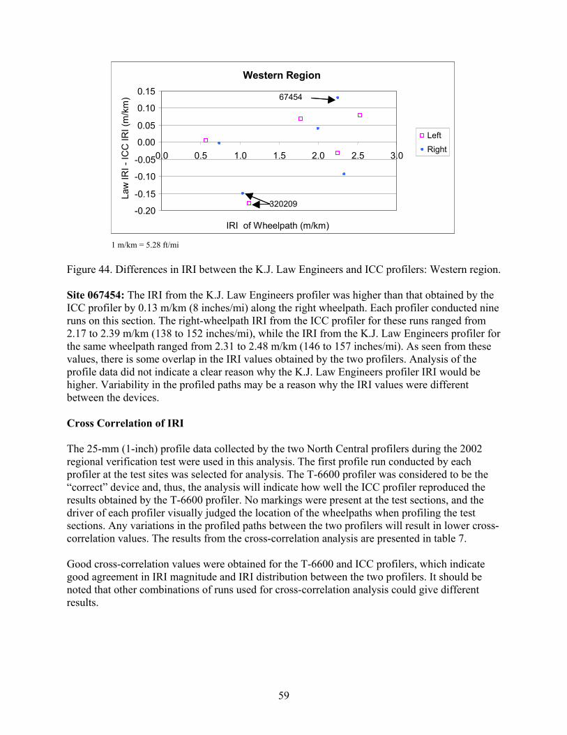
Western Region

-0.20

-0.15

-0.10

-0.05

0.00

0.05

0.10

0.15

0.0 0.5 1.0 1.5 2.0 2.5 3.0

IRI of Wheelpath (m/km)

Law

IRI -

ICC

IRI (

m/k

m)

Left

Right

320209

67454

Western Region

-0.20

-0.15

-0.10

-0.05

0.00

0.05

0.10

0.15

0.0 0.5 1.0 1.5 2.0 2.5 3.0

IRI of Wheelpath (m/km)

Law

IRI -

ICC

IRI (

m/k

m)

Left

Right

320209

67454

1 m/km = 5.28 ft/mi

Figure 44. Differences in IRI between the K.J. Law Engineers and ICC profilers: Western region.

Site 067454: The IRI from the K.J. Law Engineers profiler was higher than that obtained by the ICC profiler by 0.13 m/km (8 inches/mi) along the right wheelpath. Each profiler conducted nine runs on this section. The right-wheelpath IRI from the ICC profiler for these runs ranged from 2.17 to 2.39 m/km (138 to 152 inches/mi), while the IRI from the K.J. Law Engineers profiler for the same wheelpath ranged from 2.31 to 2.48 m/km (146 to 157 inches/mi). As seen from these values, there is some overlap in the IRI values obtained by the two profilers. Analysis of the profile data did not indicate a clear reason why the K.J. Law Engineers profiler IRI would be higher. Variability in the profiled paths may be a reason why the IRI values were different between the devices. Cross Correlation of IRI The 25-mm (1-inch) profile data collected by the two North Central profilers during the 2002 regional verification test were used in this analysis. The first profile run conducted by each profiler at the test sites was selected for analysis. The T-6600 profiler was considered to be the “correct” device and, thus, the analysis will indicate how well the ICC profiler reproduced the results obtained by the T-6600 profiler. No markings were present at the test sections, and the driver of each profiler visually judged the location of the wheelpaths when profiling the test sections. Any variations in the profiled paths between the two profilers will result in lower cross-correlation values. The results from the cross-correlation analysis are presented in table 7. Good cross-correlation values were obtained for the T-6600 and ICC profilers, which indicate good agreement in IRI magnitude and IRI distribution between the two profilers. It should be noted that other combinations of runs used for cross-correlation analysis could give different results.

59

Table 7. Results of cross correlation between the K.J. Law Engineers T-6600 and ICC profilers.

Site IRI (m/km) Cross Correlation Left Wheelpath Right Wheelpath Left Right K.J. Law ICC K.J. Law ICC Wheelpath Wheelpath

1: Asphalt 1.05 0.96 1.19 1.20 0.81 0.94 2: Asphalt 2.71 2.86 2.87 2.72 0.91 0.91 3: Concrete 1.11 1.10 1.18 1.19 0.82 0.80 4: Concrete 4.02 4.11 4.14 4.19 0.91 0.93 5: Chip Seal 3.39 3.01 3.85 4.00 0.78 0.85

1 m/km = 5.28 ft/mi ANOVA and Regression Analysis of IRI An ANOVA was performed using the IRI data obtained from the 2002 regional verification test. There were 23 sites used for testing, and this provided data for 46 cases (23 sites x 2 wheelpaths per site) where an IRI comparison could be performed for the K.J. Law Engineers and ICC profilers. For each case, IRI values for five repeat runs were available for both the ICC and K.J. Law Engineers profilers. The ANOVA indicated that the profilers were not significant at a significance level of 0.05. A regression analysis was performed for the IRI from the T-6600 and ICC profilers. The IRI for the five runs that were selected at each section to compute the average IRI value for the IRI comparison of the two profilers were used in the regression. This provided 230 pairs of data for the regression (i.e., 23 sections x 2 wheelpaths x 5 repeat runs). The following relationship was obtained from the regression:

(2) IRI (ICC) = 1.006 IRI (K.J. Law) – 0.018 where:

• IRI (ICC) = IRI from ICC profiler for a wheelpath (m/km). • IRI (K.J. Law) = IRI from K.J. Law Engineers T-6600 profiler for a wheelpath (m/km). • R2 = 0.96, standard error = 0.17.

The regression equation indicated very good agreement in IRI between the two profilers. EFFECTS OF APPLYING A MOVING AVERAGE ONTO PROFILE DATA The DNC 690 profilers collected profile data at 25.4-mm (1-inch) intervals and then applied a 304.8-mm (12-inch) moving average onto the data and recorded profile data at 152.4-mm (6-inch) intervals. Profile data collected at 25-mm (1-inch) intervals at LTPP test sections are available for both the T-6600 and ICC profilers. However, currently, in the LTPP program, these 25-mm (1-inch) profile data are processed using the ProQual software, which applies a 300-mm

60

(11.8-inch) moving average onto the 25-mm (1-inch) profile data, and extracts profile data at 150-mm (5.9-inch) intervals. The IRI values for the LTPP sections are computed using this averaged data, and the averaged data are uploaded to the LTPP database. The application of the 300-mm (11.8-inch) moving average onto the 25-mm (1-inch) data attenuates very short-wavelength features that are present in the profile, and can also distort profile features that are actually present in the pavement. The averaged profile can show features that do not actually appear in the pavement, while not showing features that are actually present in the pavement. In this section, several examples that show the distortion caused in profile features by the application of the moving average are presented. Faulted Pavement Figure 45 shows how the application of the moving average distorts the profile data collected over a fault. This figure shows the 25-mm (1-inch) interval data collected by the North Central T-6600 profiler over a faulted crack at the rough PCC section during the 1996 profiler verification study. The averaged data also are shown in this figure. The 25-mm (1-inch) data clearly define the fault, which is about 13 mm (0.5 inches). However, the application of the moving average makes the fault appear as a ramp, where there is a gradual change in elevation of about 7 mm (0.3 inches) that occurs over a distance of 0.3 m (1 ft). As seen in this example, the application of the moving average distorts the profile and shows a feature that does not actually exist on the pavement.

-20

-15

-10

-5

0136 136.5 137 137.5

Distance (m)

Ele

vatio

n (m

m)

25 mm

150 mm

25.4 mm = 1 inch 1 m = 3.28 ft

Figure 45. Profile distortion caused by the application of a moving average onto data collected over a fault.

Effects of Downward Features The rough AC section that was used in the 2003 LTPP profiler comparison conducted in Minnesota had cracks that had been patched full width across the lane. Figure 46 shows the profile data obtained by the North Atlantic ICC profiler over such a patched crack. The figure

61

shows the 25-mm (1-inch) data and the averaged data after the 25-mm (1-inch) data were processed using ProQual. The 25-mm (1-inch) data indicate that the patched crack is about 9 mm (0.4 inches) deeper than the adjacent pavement area. The application of the moving average onto the 25-mm (1-inch) data causes the depth of the patched crack to be reduced.

Distance (m)

-14

-12

-10

-8

-6

-4

-2

0128 128.5 129 129.5 130

Ele

vatio

n (m

m)

25-mm Data

Averaged 150 mm

25.4 mm = 1 inch 1 m = 3.28 ft

Figure 46. Profile distortion caused by the application of a moving average onto data collected over a patched crack.

Figure 47 shows the 25-mm (1-inch) data and the averaged 150-mm (5.9-inch) interval data at the chip-seal section that was used in the 2003 LTPP profiler comparison. These data were collected by the North Atlantic ICC profiler. The 25-mm (1-inch) data show a crack that is at a distance of about 0.9 m (3 ft) as a sharp and narrow downward feature. However, the averaged data distorts the shape of the crack and makes the crack appear as a dip that is spread over a much wider length. The small variations between the profile data points that are seen in the 25-mm (1-inch) data are not seen in the averaged data. These variations are smoothed out by the application of the moving average.

62

Distance (m)

-24

-22

-20

-18

-16

-14

-120.5 0.7 0.9 1.1 1.3 1.5

Ele

vatio

n (m

m)

25-mm DataAveraged 150 mm

25.4 mm = 1 inch

Figure 47. Profile distortion caused by the application of a moving average onto data collected over a crack.

1 m = 3.28 ft

Figure 48 shows profile data collected by the Western ICC profiler at site 3, which is a concrete section, during the 2003 profiler comparison in Minnesota. This figure shows both the 25-mm (1-inch) data and the averaged data after the 25-mm (1-inch) data were processed using ProQual. The 25-mm (1-inch) data clearly show the locations of the joints in the concrete pavement as downward spikes that occur at regular intervals. However, these features are not seen in the averaged profile because the averaging process attenuates the sharp downward features seen at the joints.

63

0

5

10

15

20

25

30

35

0 50 100 150Distance (m)

Ele

vatio

n (m

m)

25 mm

Averaged 150 mm

Profiles Offset

25 mm

Averaged 150 mm

25.4 mm = 1 inch 1 m = 3.28 ft

Figure 48. Application of a moving average onto data collected for a concrete pavement.

Effects of Sharp Upward Features Figure 49 shows a portion of the profile data collected by the North Central T-6600 profiler at section 3, which is a PCC section, during the 1996 regional verification test. The figure shows the 25-mm (1-inch) data and the averaged data after ProQual had processed the 25-mm (1-inch) data. The profile contains a sharp upward feature about 2.5 mm (0.1 inch) in height near 62 m (203 ft). The application of the moving average eliminates this feature. The application of a moving average onto a sharp upward feature that has a greater magnitude than the shown feature will cause the feature to appear in the averaged data as a feature that has a much lesser magnitude that is spread out over a much greater distance than the actual feature. The profile shown in figure 49 also shows a narrow downward feature between 65 and 66 m (213 and 216 ft). This feature also does not appear in the averaged data. Smooth Asphalt Pavement Figure 50 shows a plot that contains profile data at 25-mm (1-inch) intervals, and the same data after it had been processed using ProQual. The profile shown in figure 50 contains data collected by the Western profiler along the left wheelpath at the smooth AC site during the 2003 LTPP profiler comparison. This pavement section is a smooth pavement, and there is no distress within the limits of the profile plot shown in figure 50. Both the 25-mm (1-inch) data and the averaged 150-mm (5.9-inch) data overlay well, except that the small spike seen at 16 m (52 ft) does not appear in the averaged data.

64

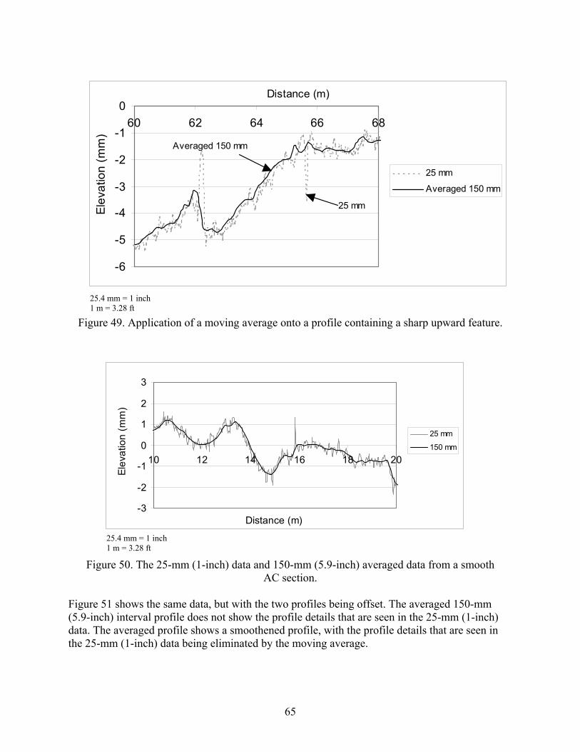
Distance (m)

-6

-5

-4

-3

-2

-1

060 62 64 66 68

Elev

atio

n (m

m)

25 mm

Averaged 150 mm

Averaged 150 mm

25 mm

25.4 mm = 1 inch 1 m = 3.28 ft

Figure 49. Application of a moving average onto a profile containing a sharp upward feature.

-3

-2

-1

0

1

2

3

10 12 14 16 18 20

Distance (m)

Elev

atio

n (m

m)

25 mm

150 mm

25.4 mm = 1 inch 1 m = 3.28 ft

Figure 50. The 25-mm (1-inch) data and 150-mm (5.9-inch) averaged data from a smooth AC section.

Figure 51 shows the same data, but with the two profiles being offset. The averaged 150-mm (5.9-inch) interval profile does not show the profile details that are seen in the 25-mm (1-inch) data. The averaged profile shows a smoothened profile, with the profile details that are seen in the 25-mm (1-inch) data being eliminated by the moving average.

65

SUMMARY OF THE FINDINGS Data recorded by inertial profilers do not accurately portray very narrow features such as cracks or joints in PCC pavements because of the low-pass filtering that is performed on the data. Evaluation of 25-mm (1-inch) data collected by both the T-6600 and ICC profilers over a joint in a PCC pavement showed that the joint appeared in the profile as a feature that was spread over a distance of 75 mm (3 inches), when the width of the joint was actually closer to 10 mm (0.4 inches). Although 25-mm (1-inch) interval data are collected by both the T-6600 and ICC profilers, the height sensors in the profilers collect data at much closer intervals and then average the data when computing profile data at 25-mm (1-inch) intervals. This causes the magnitude of a narrow feature that is recorded in the profile to be less than the actual magnitude, and also causes it to be spread out over a much wider distance than the actual feature. The application of an anti-aliasing filter onto the profile data can also have the same effect.

-3

-2

-1

0

1

2

3

4

5

10 12 14 16 18 20

Distance (m)

Elev

atio

n (m

m)

25 mm

Averaged 150 mm

25 mm

Averaged 150 mm

Profiles Offset

25.4 mm = 1 inch 1 m = 3.28 ft

Figure 51. Offset profile plot of 25-mm (1-inch) data and averaged 150-mm (5.9-inch) data collected from a smooth AC pavement.

Since the DNC 690 profiler recorded profile data at 152.4-mm (6-inch) intervals, when comparing data from the T-6600 profiler with the DNC 690 profiler, only the 150-mm (5.9-inch) interval ProQual-processed data from the T-6600 profiler can be used to perform a meaningful comparison. Comparison of the profile plots for the two profilers showed good agreement, although there were some differences between the profiles for sections that had significant long-wavelength content. This difference is attributed to the different long-wavelength cutoff filter values used for the two profilers (91 m (300 ft) for the DNC 690 profiler and 100 m (328 ft) for the T-6600 profiler). An evaluation of the profile data indicated that the long-wavelength cutoff filtering technique used in both the DNC 690 and T-6600 profilers appears to be similar. There was very good agreement in IRI values for the DNC 690 and T-6600 profilers. Since 25-mm (1-inch) interval data were available for both the T-6600 and ICC profilers, a comparison of 25-mm (1-inch) interval data for the two profilers could be performed. Evaluation

66

of the profile data using PSD plots indicated that there was good agreement in the profile data for the two profilers for wavelengths between 1 and 40 m (3 and 131 ft). For wavelengths less than 1 m (3 ft), the ICC profiler usually showed a higher wavelength content than the T-6600 profiler. This is attributed to the smaller footprint of the ICC profiler, which probably caused more texture effects and the higher magnitude of narrow features to be recorded. For wavelengths greater than 40 m (131 ft), the T-6600 profiler recorded more wavelength content than the ICC profiler. This is attributed to differences in the long-wavelength filtering techniques that are used by the two profilers. When ProQual-processed data for the two profilers were compared using a PSD plot, only the differences at the higher wavelengths will be seen, with good agreement being obtained between the two profilers for wavelengths less than 1 m (3 ft). This occurs because the application of the moving average attenuates the short-wavelength features. Good agreement in IRI, which is primarily influenced by wavelengths between 1 and 30 m (3 and 100 ft), was obtained for data collected by the ICC and T-6600 profilers. In the LTPP program, the 25-mm (1-inch) data obtained from the T-6600 and ICC profilers are processed using ProQual. ProQual applies a 300-mm (11.8-inch) moving average onto the 25-mm (1-inch) data and extracts data at 150-mm (5.9-inch) intervals, and these data are uploaded to the LTPP database. The application of the moving average onto the 25-mm (1-inch) data attenuates features with wavelengths less than 1 m (3 ft). Detailed profile features cannot be observed in the ProQual-processed data because of this effect. The moving average can also distort the profile data, with the averaged data showing features that are not actually present in the pavement, while eliminating features that are actually present.

67

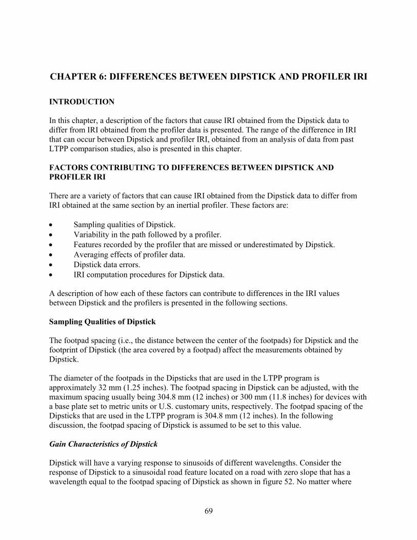
CHAPTER 6: DIFFERENCES BETWEEN DIPSTICK AND PROFILER IRI

INTRODUCTION In this chapter, a description of the factors that cause IRI obtained from the Dipstick data to differ from IRI obtained from the profiler data is presented. The range of the difference in IRI that can occur between Dipstick and profiler IRI, obtained from an analysis of data from past LTPP comparison studies, also is presented in this chapter. FACTORS CONTRIBUTING TO DIFFERENCES BETWEEN DIPSTICK AND PROFILER IRI There are a variety of factors that can cause IRI obtained from the Dipstick data to differ from IRI obtained at the same section by an inertial profiler. These factors are: • Sampling qualities of Dipstick. • Variability in the path followed by a profiler. • Features recorded by the profiler that are missed or underestimated by Dipstick. • Averaging effects of profiler data. • Dipstick data errors. • IRI computation procedures for Dipstick data. A description of how each of these factors can contribute to differences in the IRI values between Dipstick and the profilers is presented in the following sections. Sampling Qualities of Dipstick The footpad spacing (i.e., the distance between the center of the footpads) for Dipstick and the footprint of Dipstick (the area covered by a footpad) affect the measurements obtained by Dipstick. The diameter of the footpads in the Dipsticks that are used in the LTPP program is approximately 32 mm (1.25 inches). The footpad spacing in Dipstick can be adjusted, with the maximum spacing usually being 304.8 mm (12 inches) or 300 mm (11.8 inches) for devices with a base plate set to metric units or U.S. customary units, respectively. The footpad spacing of the Dipsticks that are used in the LTPP program is 304.8 mm (12 inches). In the following discussion, the footpad spacing of Dipstick is assumed to be set to this value. Gain Characteristics of Dipstick Dipstick will have a varying response to sinusoids of different wavelengths. Consider the response of Dipstick to a sinusoidal road feature located on a road with zero slope that has a wavelength equal to the footpad spacing of Dipstick as shown in figure 52. No matter where

69

Dipstick is placed on this sinusoid, Dipstick will give a reading of zero, because the two supporting feet will have the same elevation. Dipstick measurements taken along a roadway that has such a feature will not capture the feature, and will simply give a straight line for the elevation profile. In the case of a road with a slope that has such a feature, the Dipstick measurements will only show the slope of the road, and will not show the sinusoidal feature present on the road.

Figure 52. Dipstick response to a sinusoid with a wavelength equal to the footpad spacing of Dipstick.

The response of Dipstick to different wavelengths can be studied by using a gain plot. The following procedure is used to generate the gain plot: 1. Select a sinusoid that has a specific wavelength and specific amplitude. Assume that the

amplitude of the sinusoid is A. 2. Simulate placing Dipstick at the start of the sinusoid and compute the reading that would

be obtained by Dipstick (i.e., the difference in elevation between the front and back footpads).

3. Again place Dipstick on the sinusoid so that the current position of Dipstick is slightly

ahead (e.g., 25 mm (1 inch)) of the previous location. Compute the reading that would be obtained by Dipstick. Repeat this procedure until Dipstick has been placed for all positions in the sinusoid, covering an entire wavelength.

4. After completing this exercise, use the readings that Dipstick obtained for each Dipstick

position to generate the profile (sinusoid) that was recorded by Dipstick. 5. Divide the maximum amplitude of the generated profile by the amplitude of the sinusoid

that was used to generate this profile (i.e., A) to obtain the gain for that wavelength.

70

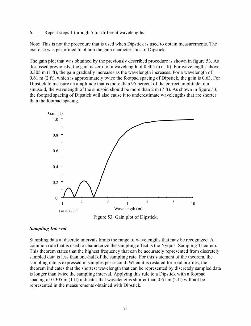
6. Repeat steps 1 through 5 for different wavelengths. Note: This is not the procedure that is used when Dipstick is used to obtain measurements. The exercise was performed to obtain the gain characteristics of Dipstick. The gain plot that was obtained by the previously described procedure is shown in figure 53. As discussed previously, the gain is zero for a wavelength of 0.305 m (1 ft). For wavelengths above 0.305 m (1 ft), the gain gradually increases as the wavelength increases. For a wavelength of 0.61 m (2 ft), which is approximately twice the footpad spacing of Dipstick, the gain is 0.63. For Dipstick to measure an amplitude that is more than 95 percent of the correct amplitude of a sinusoid, the wavelength of the sinusoid should be more than 2 m (7 ft). As shown in figure 53, the footpad spacing of Dipstick will also cause it to underestimate wavelengths that are shorter than the footpad spacing.

.1 2 5 1 2 5 10Wavelength (m)

0

0.2

0.4

0.6

0.8

1.0Gain (1)

1 m = 3.28 ft

Figure 53. Gain plot of Dipstick. Sampling Interval Sampling data at discrete intervals limits the range of wavelengths that may be recognized. A common rule that is used to characterize the sampling effect is the Nyquist Sampling Theorem. This theorem states that the highest frequency that can be accurately represented from discretely sampled data is less than one-half of the sampling rate. For this statement of the theorem, the sampling rate is expressed in samples per second. When it is restated for road profiles, the theorem indicates that the shortest wavelength that can be represented by discretely sampled data is longer than twice the sampling interval. Applying this rule to a Dipstick with a footpad spacing of 0.305 m (1 ft) indicates that wavelengths shorter than 0.61 m (2 ft) will not be represented in the measurements obtained with Dipstick.

71

The sampling interval of Dipstick also may cause features with wavelengths shorter than twice the sampling interval to contaminate the measurement of longer wavelength features through a process called aliasing. Aliasing occurs when short-wavelength features are inadvertently interpreted to be longer wavelength features. For example, consider a sinusoid with a wavelength that is 11 percent longer than the sampling interval of Dipstick, as shown in figure 54. The first sample detects the highest point in the sinusoid; however, each successive point misses the peak by a progressively greater distance. The consequence is a gradual transition from the peak level to the valley over a long distance. Thus, a Dipstick having a sampling interval of 0.305 m (1 ft) that is measuring a sinusoid with a wavelength of 0.339 m (1.1 ft) would obtain a sinusoid of roughly equal amplitude, but having a wavelength of 3.05 m (10 ft).

Figure 54. An example of aliasing. In cases where the wavelength of the sinusoid is shorter than the sampling interval of Dipstick, a much longer wavelength than that actually present also will appear in the measurement. For example, a sinusoid with a wavelength that is 10 percent shorter than the sampling interval would also be misinterpreted as a feature with a wavelength of about 3.05 m (10 ft). On the other hand, features with wavelengths that are just shorter than double the sampling interval will be aliased into features with wavelengths that are just longer than twice the sampling interval. The way to avoid aliasing errors is to sample much more often than the shortest wavelength of interest, then apply a low-pass filter to remove the contents within the signal that are not of interest. However, such a procedure cannot be used with the Dipstick. The overall consequence of aliasing by Dipstick is that contents within the profile in a wavelength range shorter than 0.61 m (2 ft) are “folded” into the longer wavelength range. This causes an upward bias in the IRI value by artificially increasing the contents within the profile that fall within the wavelength range that affects IRI. The precise level of upward bias depends on the properties of the road surface, and this effect is much greater on pavement with a high level of megatexture or coarse macrotexture. The probable effect of aliasing on IRI for a sampling interval of 0.3 m (1 ft) was estimated in a recent study of profile sampling procedures.(1) This study showed that the upward bias in IRI because of aliasing is probably on the order of 7 to 9 percent. The probable error level in this study was estimated by decimating profiles collected with the FHWA PRORUT profiler at two test sections. It should be noted that the treatment of very short road features by the feet of

72

Dipstick might be different than the procedure used by the sensor footprint of the profiler. The anti-aliasing that had been used for the profile that was used in the study may impact the conclusions of that study. It should also be noted that data from only two sites were used in this analysis. Therefore, the 7 to 9 percent error level is only a rough estimate. Dipstick Footprint Dipstick contacts the pavement at two locations (spaced 304.8 mm (12 inches) apart) with rigid circular feet that are approximately 32 mm (1.25 inches) in diameter. The feet are attached to the base of Dipstick with a ball joint so that the footpads are most likely to rest upon the three highest points within the footprint of the footpad. An important property of this type of footprint is the ability to bridge over narrow cracks and rest on small pieces of protruding aggregate. If the macrotexture is not very deep, the footprint may serve as a mechanical filter that removes the potential for aliasing error caused by wavelengths on the order of 32 mm (1.25 inches) and shorter. Variations in the Path Followed by the Profiler During profiler comparison studies, Dipstick measurements at test sections are performed along the two wheelpaths. In LTPP comparison experiments, the wheelpaths are laid out so that each wheelpath is at a distance of 0.826 m (2.7 ft) from the center of the lane.(6) Where wheelpaths are easily identified, the midway point between the two wheelpaths is defined to be the center of the lane. If the wheelpaths cannot be clearly identified, but the two lane edges are well defined, the center of the travel lane is considered to be midway between the lane edges. Chalk lines are laid out along the wheelpaths when performing Dipstick measurements. The wheelpaths were marked with paint dots at all sections during the 1991 and 2003 LTPP profiler comparisons, while two sections used for the 2000 LTPP profiler comparison had the wheelpaths marked. The paint dots provided a guide so that the driver could align the profiler along the wheelpaths when profiling the test sections. During other LTPP profiler comparisons, the drivers had to judge the location of the wheelpath when profiling the test sections. If the profiler driver does not align the profiler along the wheelpaths, the longitudinal path that is followed by the sensors in the profiler will be different from the path where Dipstick measurements were obtained. Also, if the profiler driver does not consistently follow the wheelpaths within the section, but has some lateral wander, this will result in differences in the paths measured by the profiler and Dipstick. Both of these conditions can cause IRI obtained from profiler measurements to differ from that obtained from Dipstick measurements. A discussion of lateral wander and the effects on IRI were presented in chapter 5. As shown in table 3, at some sections, lateral wander can have a significant effect on IRI. Figure 55 shows the 10-m (33-ft) base-length roughness profiles for the left wheelpath obtained for nine repeat runs performed by the Western profiler at test section 1, which is a smooth AC section, during the 2003 LTPP profiler comparison in Minnesota. The roughness profiles overlay very well, with the IRI for the entire section for the nine runs ranging from 1.29 to 1.33 m/km (82 to 84 inches/mi). The roughness profiles imply that either the profiler driver followed the

73

same path for all nine runs or that minor variations in the wheelpath during profiling did not affect IRI.

10-m Roughness Profiles

0.0

0.5

1.0

1.5

2.0

2.5

3.0

0 20 40 60 80 100 120 140Distance (m)

IRI (

m/k

m)

1 m = 3.28 ft 1 m/km = 5.28 ft/mi

Figure 55. Roughness profiles for nine runs that show good agreement. Thus, if the driver was tracking the wheelpath correctly, close agreement between profiler IRI and Dipstick IRI is expected at this site. However, the Dipstick IRI for the left wheelpath was 1.17 m/km (74 inches/mi), which is less than the IRI obtained from the profiler data. A comparison of the roughness profiles obtained by the profiler and Dipstick showed that the roughness profiles were different in a few localized areas. An evaluation of the profiles indicated that the profiler data had a deep narrow feature that was not captured by the Dipstick measurements, and omission of this feature in the Dipstick data was the primary reason why the IRI from the Dipstick data was lower than the IRI from the profiler data for this section. Figure 56 shows the 10-m (33-ft) base-length roughness profiles along the right wheelpath for two runs of the Western profiler at test section 1, which is a smooth AC section, during the 2003 LTPP profiler comparison that was held in Minnesota. The two roughness profiles show good agreement, except at three high roughness locations: (1) between 40 and 50 m (131 and 164 ft), (2) between 60 and 75 m (197 and 245 ft), and (3) between 85 and 100 m (279 and 328 ft). IRI for the two runs shown in this figure are 1.62 m/km (103 inches/mi) for run 4 and 1.79 m/km (113 inches/mi) for run 2. The difference in the IRI between the two runs occurs because of differences in the pavement features that are measured during the two runs within the three rough areas that were described previously. Therefore, variations in the path profiled at this site can have a significant influence on the IRI obtained for the right wheelpath. At sites having such characteristics, variations in the path profiled by the profiler compared to the path where Dipstick data were collected can cause significant differences between profiler IRI and Dipstick IRI. Figure 57 shows 10-m (33-ft) base-length roughness profiles for a single run by the North Atlantic, North Central, and Western profilers along the left wheelpath of section 4, which is a PCC section that was used for the 2003 LTPP profiler comparison.

74

10-m Roughness Profiles

0.00.51.01.52.02.53.03.54.0

0 20 40 60 80 100 120 140

Distance (m)

IRI (

m/k

m)

Run 2Run 4

1 m = 3.28 ft 1 m/km = 5.28 ft/mi

Figure 56. Roughness profiles for two profile runs that show variations.

10-m Roughness Profiles

0.0

0.5

1.0

1.5

2.0

2.5

3.0

3.5

0 25 50 75 100 125 150Distance (m)

IRI (

m/k

m)

N. AtlanticN. CentralWestern

N. CentralN. Atlantic

Western

1 m = 3.28 ft 1 m/km = 5.28 ft/mi

Figure 57. Roughness profiles along the left wheelpath for three profilers. The roughness profiles from the three profilers agree well with each other throughout the section, except between 25 and 40 m (82 and 131 ft). This indicates that variations in the path followed by the three profilers within these limits are causing differences in the pavement features that are measured. This will cause different IRI values to be obtained for this wheelpath by the three profilers. Thus, IRI obtained by the three profilers will differ from that obtained by Dipstick. Features Recorded by the Profiler That Are Missed or Underestimated by Dipstick

75

Dipstick obtains measurements at 304.8-mm (12-inch) intervals and is equipped with footpads that are 32 mm (1.25 inches) in diameter. The profilers that have a recording interval of 25 mm (1 inch) will record 12 measurements within the distance between the Dipstick footpads. Thus, Dipstick can miss features that are measured by a profiler. In addition, Dipstick will not measure narrow cracks or joints in a PCC pavement when a Dipstick footpad is placed over such a feature, since the footpad will bridge over such features. However, a profiler will measure such features. When computing IRI, the IRI algorithm will treat a narrow downward feature the same as if that feature were upward. Features missed because of the footpad spacing and bridging over of narrow downward features can cause IRI obtained from Dipstick measurements to be less than that obtained from profiler measurements. Figure 58 shows profile plots for (1) data collected along the left wheelpath at section 5 (chip-seal section) during the 2003 LTPP profiler comparison by the North Atlantic ICC profiler at 25-mm (1-inch) intervals, (2) the same data after being processed using ProQual (i.e., moving average applied), and (3) data collected by Dipstick after all data sets have been subjected to a 3-m (10-ft) high-pass filter. When the 25-mm (1-inch) profile data are processed using ProQual, the depth of the cracks in the resulting averaged profile will be attenuated. Also, narrow cracks that appear in the 25-mm (1-inch) data will be more spread out, and can appear as a slight dip rather than a narrow crack.

3-m High Pass Filtered

0

5

10

15

20

25

30

110 120 130 140Distance (m)

Ele

vatio

n (m

m)

Figure 58. Measurement of cracks by a profiler and Dipstick. At a distance of 120.5 m (395 ft), there is a crack in the pavement that is seen in the profile data; however, this crack is not seen in the Dipstick data, either because the Dipstick footpad bridged the crack or the crack was between the contact points of the Dipstick footpad. Sometimes the pavement area adjacent to a crack has a slight dip because of settlement close to the crack. If the footpad of Dipstick falls within this settled area, the Dipstick profile will show a slight dip at such locations. The Dipstick profile shown in figure 58 does show a slight dip close to many

Top - 25 mm

Middle - 150 mm

Bottom - Dipstick

3-m High-Pass Filtered

Profiles Offset25 mm

150 mm

Dipstick

25.4 mm = 1 inch 1 m = 3.28 ft

76

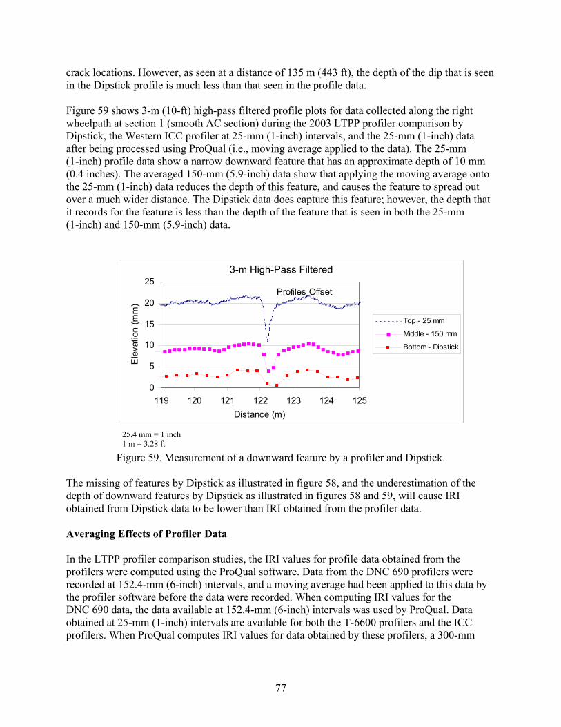
crack locations. However, as seen at a distance of 135 m (443 ft), the depth of the dip that is seen in the Dipstick profile is much less than that seen in the profile data. Figure 59 shows 3-m (10-ft) high-pass filtered profile plots for data collected along the right wheelpath at section 1 (smooth AC section) during the 2003 LTPP profiler comparison by Dipstick, the Western ICC profiler at 25-mm (1-inch) intervals, and the 25-mm (1-inch) data after being processed using ProQual (i.e., moving average applied to the data). The 25-mm (1-inch) profile data show a narrow downward feature that has an approximate depth of 10 mm (0.4 inches). The averaged 150-mm (5.9-inch) data show that applying the moving average onto the 25-mm (1-inch) data reduces the depth of this feature, and causes the feature to spread out over a much wider distance. The Dipstick data does capture this feature; however, the depth that it records for the feature is less than the depth of the feature that is seen in both the 25-mm (1-inch) and 150-mm (5.9-inch) data.

Figure 59. Measurement of a downward feature by a profiler and Dipstick.

he missing of features by Dipstick as illustrated in figure 58, and the underestimation of the

veraging Effects of Profiler Data

the LTPP profiler comparison studies, the IRI values for profile data obtained from the re

y

ata

3-m High Pass Filtered

0

5

10

15

20

25

119 120 121 122 123 124 125Distance (m)

Ele

vatio

n (m

m)

Tdepth of downward features by Dipstick as illustrated in figures 58 and 59, will cause IRI obtained from Dipstick data to be lower than IRI obtained from the profiler data. A Inprofilers were computed using the ProQual software. Data from the DNC 690 profilers werecorded at 152.4-mm (6-inch) intervals, and a moving average had been applied to this data bthe profiler software before the data were recorded. When computing IRI values for the DNC 690 data, the data available at 152.4-mm (6-inch) intervals was used by ProQual. Dobtained at 25-mm (1-inch) intervals are available for both the T-6600 profilers and the ICC profilers. When ProQual computes IRI values for data obtained by these profilers, a 300-mm

Top - 25 mm

Middle - 150 mm

Bottom - Dipstick

3-m High-Pass Filtered

Profiles Offset

25.4 mm = 1 inch 1 m = 3.28 ft

77

(11.8-inch) moving average is first applied to the data, then profile data points that are at 150-mm (5.9-inch) intervals are extracted and the IRI is computed using this averaged data. The effects of application of the moving average onto the 25-mm (1-inch) data were discussed in chapter 5. The averaged profile obtained from the profiler data that are used for computation of IRI by ProQual is an artificial profile, and this profile may not actually exist on the road. However, when measurements are performed with Dipstick, readings will be obtained on the actual profile of the road. For example, consider the profiles shown in figure 60 that show the 25-mm (1-inch) profile data, and the profile obtained after ProQual has processed the 25-mm (1-inch) data. When computing IRI for profile data, the 150-mm (5.9-inch) interval profile, which is an artificial profile, is used. However, when Dipstick obtains readings, the footpads of Dipstick will rest on the actual profile of the pavement, and not on the artificial profile that is defined by the 150-mm (5.9-inch) interval profile. Thus, this difference in the profiles between the profiler data and the Dipstick data can result in differences in the IRI values.

-20

-15

-10

-5

0

5

136 136.5 137 137.5

Distance (m)

Ele

vatio

n (m

m)

25 mm 150 mm

25.4 mm = 1 inch 1 m = 3.28 ft

Figure 60. Illustration of artificial profile used by ProQual for computing IRI. For asphalt-surfaced pavements without distress, the difference between the averaged profile computed using ProQual and the profile defined by the 25-mm (1-inch) data will be very minor, and the two profiles may actually coincide. However, in new PCC pavements, there could be differences between these two profiles at the joints. The 25-mm (1-inch) profile will show the joint as a downward feature; however, this feature may not be seen in the averaged profile computed using ProQual, since it is smoothed out when the moving average is applied. On pavements that have distress, there could be significant differences between the 25-mm (1-inch) interval profile and the 150-mm (5.9-inch) interval averaged profile. Dipstick Data Errors In the LTPP program, when longitudinal Dipstick measurements are performed, the Dipstick readings are recorded on a form. Afterwards, these readings are entered into ProQual to compute

78

the IRI. After Dipstick measurements are performed in the field, a closure error computation is performed as a data quality check.(6) Although this procedure does provide a check on the data quality, it is always possible for errors during measurement to occur, yet the closure error may be within the acceptable value. Also, multiple errors may occur that compensate for each other and cause the closure error to be within the acceptable value. Figure 61 shows the 10-m (33-ft) base-length roughness profiles obtained along the left wheelpath at site 5 (chip-seal section) during the 2003 LTPP profiler comparison for a run by the Western profiler and Dipstick. There are differences between the two roughness profiles, with Dipstick showing much higher roughness than the profiler between 20 and 30 m (66 and 100 ft). This indicates that Dipstick is capturing a feature between these limits that is causing a high roughness, and this feature is not appearing in the profile data collected by the profiler.

10-m Roughness Profiles

0.00.51.01.52.02.53.03.54.0

0 20 40 60 80 100 120 140Distance (m)

IRI (

m/k

m)

ProfilerDipstick

Dipstick Profiler

1 m = 3.28 ft 1 m/km = 5.28 ft/mi

Figure 61. Left-wheelpath 10-m (33-ft) base-length roughness profiles for profiler and Dipstick at site 5.

Figure 62 shows the 10-m (33-ft) high-pass filtered profiles of the profiler and Dipstick at this site from the start of the section to a distance of 50 m (164 ft). This figure shows that at an approximate distance of 22 m (72 ft), a sharp upward feature is seen in the Dipstick profile; however, this feature does not appear in the profile recorded by the profiler. This is the feature that caused the Dipstick roughness profile to show a higher value than the profiler roughness profile between the limits of 20 and 30 m (66 and 100 ft). This particular feature did not appear in any of the profile data collected by all of the profilers at this site.

Since this feature did not appear in the profile data collected by any profiler, the sharp upward nature of the feature indicates that it is most likely an erroneous data point. The possible reason for this feature appearing in the Dipstick data is either: (1) an incorrect reading being recorded at that location in the field, (2) an incorrect reading at that location being entered into ProQual, or (3) a Dipstick malfunction occurring at that location.

79

Figure 63 shows a portion of the right-wheelpath profile that was recorded by Dipstick and a profiler at site 1 (smooth AC section) during the 2003 LTPP profiler comparison. Both profiles have been subjected to a 10-m (33-ft) high-pass filter, and the profiles have been offset for clarity. At a distance of about 145 m (476 ft), the Dipstick profile shows a sudden drop in elevation; however, this feature is not seen in the profile recorded by the profiler. None of the profile runs for any of the profilers showed this feature in the profile. It is most likely that this feature in the Dipstick profile was caused by one of the factors that were described previously for the previous example. The inclusion of this feature in the Dipstick profile will cause an increase in the IRI for the Dipstick data.

Figure 62. Left-wheelpath profiles for profiler and Dipstick at site 5.

Figure 63. Right-wheelpath profiles for profiler and Dipstick at site 1.

10-m High Pass Filtered

0

5

10

15

20

25

30

0 10 20 30 40 50Distance (m)

Ele

vatio

n (m

m)

Top - Profiler

Bottom - Dipstick

Profiles OffsetOff t

Profiler

Dipstick

10-m High Pass Filtered

0

5

10

15

20

25

130 135 140 145 150Distance (m)

Ele

vatio

n (m

m)

25.4 mm = 1 inch 1 m = 3.28 ft

25.4 mm = 1 inch 1 m

Dipstick

ICC Profiler

Profiles Offset

1 m = 3.28 ft 1 inch = 25.4 mm

= 3.28 ft

80

At the start of the LTPP program, the data collection procedures that were employed for Dipstick

.

e

red

he two examples shown in this section illustrate errors that can occur during Dipstick data , or

I Computation Procedure for Dipstick Data

the LTPP program, the IRI values of a profile obtained from Dipstick measurements are

ed in

he correct method to accurately compute the IRI from the Dipstick data is to apply the IRI

ed

are s

est

s

16

re

calculates IRI.

data collection were different from the current procedures. In those procedures, measurements along a wheelpath were performed from the start of the section to the end of the section and, thereafter, measurements were made back along the same path to end at the start of the sectionThese procedures provided two profiles for a wheelpath, and if an error was suspected, the forward and return runs could be compared to determine whether there were differences. Thcurrent Dipstick data collection procedures where measurements are performed along a loop were adopted to save the time required to perform Dipstick measurements (and the time requiwas cut in half). However, the disadvantage of these procedures is that since only one profile is available for a wheelpath, there is no way to check whether a potentially incorrect data point is indeed incorrect. Tcollection. Such errors can occur because of a data recording error, an error during data entrya malfunction of Dipstick. If such errors occur, they will cause an upward bias in the IRI computed from the Dipstick data. IR Incomputed using the ProQual software.(7,8) The procedure used by the ProQual software to compute the IRI values from Dipstick elevation data was described in chapter 2. As describthat chapter, the Dipstick elevation profile is rotated to obtain an additional distance of 152.4 m (500 ft) before the section, the entire profile is filtered with the upper-wavelength cutoff filter used in the profiler, and then the portion of the profile corresponding to the test section is extracted from the filtered profile and the IRI is computed using this extracted profile. Talgorithm to the actual elevation profile that is obtained from the Dipstick data, and not to a filtered Dipstick profile. The analysis of the data from the LTPP profiler comparison conductin 2003 indicated that there was a slight difference in IRI values obtained when the same Dipstick elevation profile was processed using ProQual and RoadRuf. The RoadRuf softwuses the IRI computation procedure documented in American Society for Testing and Material(ASTM) Standard E1926-98 (2003).(29) RoadRuf does not perform any prefiltering of the Dipstick data before computing the IRI. Table 8 presents the IRI values obtained for four tsections in the 2003 LTPP comparison using ProQual and RoadRuf. The IRI computed using ProQual were slightly higher than that computed using RoadRuf for all of the cases by amountvarying from 0.02 to 0.08 m/km (1.3 to 5.1 inches/mi). For all practical purposes, differences of these magnitudes can be considered to be negligible. However, for LTPP comparison studies where one criterion that is being evaluated is to determine whether the profiler IRI is within 0.m/km (10 inches/mi) of the IRI obtained from Dipstick, the magnitude of the IRI differences shown in table 8 can make the difference between either satisfying or failing the criterion. Thewas perfect agreement in the IRI values that were computed for the profiler data using ProQual and RoadRuf. Therefore, a possible reason for the discrepancy in Dipstick IRI values between RoadRuf and ProQual may be the filtering that is performed on the profile data before ProQual

81

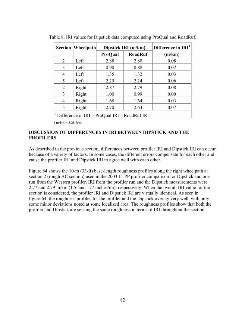
Table 8. IRI values for Dipstick data computed using ProQual and RoadRuf.

Section Wheelpath Dipstick IRI (m/km) Difference in IRI1

ProQual RoadRuf (m/km) 2 Left 2.88 2.80 0.08 3 Left 0.90 0.88 0.02 4 Left 1.35 1.32 0.03 5 Left 2.29 2.24 0.06 2 Right 2.87 2.79 0.08 3 Right 1.00 0.99 0.00 4 Right 1.68 1.64 0.03 5 Right 2.70 2.63 0.07

1 Difference in IRI = ProQual IRI – RoadRuf IRI DISCUSSION OF DIFFERENCES IN IRI BETWEEN DIPSTICK AND THE PROFILERS As described in the previous section, differences between profiler IRI and Dipstick IRI can occur because of a variety of factors. In some cases, the different errors compensate for each other and cause the profiler IRI and Dipstick IRI to agree well with each other. Figure 64 shows the 10-m (33-ft) base-length roughness profiles along the right wheelpath at section 2 (rough AC section) used in the 2003 LTPP profiler comparison for Dipstick and one run from the Western profiler. IRI from the profiler run and the Dipstick measurements were 2.77 and 2.79 m/km (176 and 177 inches/mi), respectively. When the overall IRI value for the section is considered, the profiler IRI and Dipstick IRI are virtually identical. As seen in figure 64, the roughness profiles for the profiler and the Dipstick overlay very well, with only some minor deviations noted at some localized area. The roughness profiles show that both the profiler and Dipstick are sensing the same roughness in terms of IRI throughout the section.

1 m/km = 5.28 ft/mi

82

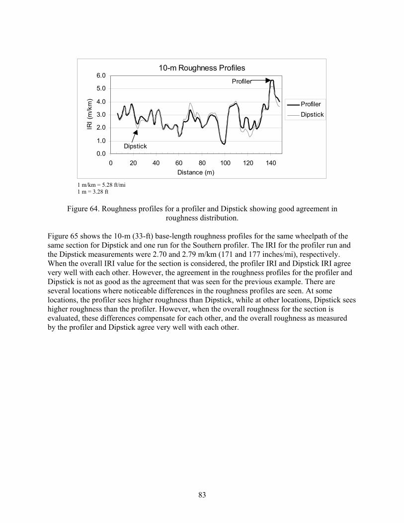
10-m Roughness Profiles

0.

6.0

0

1.

2.

3.

4.

5.0

40 6 80 120 140nce (m)

IRI (

m/k

m)

0

0

0

0

0 20 0 100Dista

ProfilerDipstick

Profiler

Dipstick

Figure 64. Roughness profiles for a profiler and Dipstick showing good agreement in

igure 65 shows the 10-m (33-ft) base-length roughness profiles for the same wheelpath of the

I and Dipstick IRI agree ery well with each other. However, the agreement in the roughness profiles for the profiler and

ees

ured

1 m/km = 5.281 m =

ft/mi 3.28 ft

roughness distribution. Fsame section for Dipstick and one run for the Southern profiler. The IRI for the profiler run and the Dipstick measurements were 2.70 and 2.79 m/km (171 and 177 inches/mi), respectively. When the overall IRI value for the section is considered, the profiler IRvDipstick is not as good as the agreement that was seen for the previous example. There are several locations where noticeable differences in the roughness profiles are seen. At some locations, the profiler sees higher roughness than Dipstick, while at other locations, Dipstick shigher roughness than the profiler. However, when the overall roughness for the section is evaluated, these differences compensate for each other, and the overall roughness as measby the profiler and Dipstick agree very well with each other.

83

The cross-correlation technique is a method that can be used to judge the agreement in IRI and the agreement in spatial distribution of IRI between two devices. The data collected for the 2003 LTPP profiler comparison by the North Atlantic and Western profilers were used with the Dipstick data to calculate cross correlation for IRI between the profilers and Dipstick. In this analysis, Dipstick was considered to be the correct device, and the analysis will indicate how well each of these profilers was able to reproduce the IRI obtained from the Dipstick measurements. The five ProQual-processed profile runs submitted by the North Atlantic and Western regions were used to calculate the cross correlation with Dipstick. The results of this analysis are presented in tables 9 and 10 for the left and right wheelpaths, respectively.

in

: Left wheelpath.

Site Profiler Cross Correlation With Dipstick

10-m Roughness Profiles

1.0

5.0

6.0

Figure 65. Roughness profiles for a profiler and Dipstick showing moderate agreementroughness distribution.

Table 9. Results of cross-correlation analysis

Run Number Minimum Maximum Average 1 2 3 4 5

1: Smooth AC North Atlantic 0.84 0.84 0.86 0.86 0.88 0.84 0.88 0.86 Western 0.82 0.83 0.83 0.84 0.84 0.82 0.84 0.84 2: Rough AC North Atlantic 0.82 0.82 0.82 0.83 0.87 0.82 0.87 0.83 Western 0.85 0.89 0.89 0.89 0.90 0.85 0.90 0.89 3: Smooth PCC North Atlantic 0.78 0.78 0.79 0.80 0.82 0.78 0.82 0.79 Western 0.82 0.82 0.83 0.84 0.84 0.82 0.84 0.83 4: Medium PCC North Atlantic 0.79 0.80 0.86 0.87 0.89 0.79 0.89 0.84 Western 0.82 0.83 0.84 0.84 0.84 0.82 0.84 0.83 5: Chip Seal North Atlantic 0.68 0.70 0.71 0.72 0.72 0.68 0.72 0.71 Western 0.69 0.70 0.72 0.73 0.73 0.69 0.73 0.71

0.00 20 40 60 80 100 120 140

Distance (m)

2.0IRI (

3.0m/k

4.0m)

ProfilerDipstick

Dipstick Profiler

1 m/km = 5.28 ft/mi 1 m = 3.28 ft

84

Table 10. Results of cross-correlation analysis: Right wheelpath.

Site Profiler Cross Correlation With Dipstick Run Number Minimum Maximum Average 1 2 3 4 5

1: Smooth AC North Atlantic 0.68 0.68 0.69 0.74 0.74 0.68 0.74 0.70 69 Western 0.62 0.65 0.70 0.72 0.77 0.62 0.77 0.2 0.83 : Rough AC North Atlantic 0.76 0.82 0.82 0.86 0.87 0.76 0.87 Western 0.67 0.70 0.70 0.74 0.75 0.67 0.75 0.71 3: Smooth PCC 0.81 North Atlantic 0.80 0.81 0.81 0.82 0.82 0.80 0.82 0.81 Western 0.80 0.81 0.81 0.81 0.83 0.80 0.83 4: Medium 0.86 PCC North Atlantic 0.85 0.85 0.85 0.87 0.87 0.85 0.87 0.88 Western 0.87 0.88 0.88 0.89 0.90 0.87 0.90 5: Chip Seal 0.78 North Atlantic 0.75 0.77 0.79 0.79 0.79 0.75 0.79 0.78 Western 0.77 0.77 0.78 0.78 0.79 0.77 0.79

0.71

the maxim

indicates tha

istribution wever, this does not necessarily mean that the runs of the profiler llowed the as measured by Dipstick.

Alo.69 (site 1) to 0.88 (site 3). For a sp fic wheelpath, the difference etween the maximum and minimum cross-correlation values for the different runs was within .05 for six cases,

two cases where t a difference of 0.15) and the North Atlantic profiler at site 2 (a tion values along the right wheelpath also general the prof ki nduring the repeat runs or that minor variati

n u o g s.

ow e lpath ction 1 f stick ae r o r the profile 0.62, w

was the lowest elatio ed in tudy. Th values a km (100 and 115 inches/mi),

respectively. M roughi the f s within these limits

differently, and lts in a low c or th devices

Figure 67 show hness e ath ion 2 fo tick anrun 5 for the Western profiler. The IRI cross correlation for this case was 0.90, which was the

Along the left wheelpath, the average cross-correlation values for the five sites ranged from(site 1) to 0.89 (site 2). For a specific profiler and a specific wheelpath, the difference between

um and minimum cross-correlation values for the different runs was within 0.05 for all of the cases, except for the North Atlantic profiler at site 4, which had a difference of 0.10. This

t the profilers are tracking a consistent path during the repeat runs or that minor variations in the wheelpaths for repeat runs are not significantly influencing the spatial d of roughness. Hofo path that w

ng the right wheelpath, the average cross-correlation values for the five sites ranged from ecific profiler and a speci0

b0 between 0.05 and 0.10 for two cases, and exceeded 0.10 for two cases. The

he value exceeded 0.10 were for the Western profiler at site 1 ( difference of 0.11). The cross-correla

ly indicate that ons in the wheelpaths for repeat runs are not

ilers are trac ng a consiste t path

significantly i

fluencing the spatial distrib tion f rou hnes

Figure 66 shrun 1 from th

s the roughness Western profiler

profil. The

es aloIRI c

ng thoss c

rightrrelat

wheeion fo

at sese two

or Dips was

nd hich

cross corr n for all of the cases consider this s e IRI for the profiler and Dipstick for this case were 1.57 nd 1.81 m/

ost of the ness at this site occurs at four localized areas, as shown in figure 66. However, the profiler and Dipst ck are measuring eature

this resu ross-correlation value f e two .

s the roug profiles along th left wheelp at sect r Dips d

85

highest cross correlation for all of the cases considered in this study. The IRI from the profiler and Dipstick for ctively. Rou profiles o devices overlay w e localized area ese c profiler an

ess

or

this case were 2.76 and 2.80 m/km (175 and 178 inches/mi), respeghnesss. t th

for the twations, the

ell within the section, except for somrded dif resA lo d Dipstick reco ferent featu .

10-m s iles

0 20 40 60 80 100 120 140

Roughnes Prof4.03.5

Figure 66. Roughness profiles for the case with the lowest cross correlation.

Figure 67. Roughness profiles for the case with the highest cross correlation. As shown in the cross-correlation study, perfect agreement in the magnitude of the roughnand spatial distribution of the roughness did not occur between the profiler and Dipstick. However, a fairly good correlation (i.e., a correlation of greater than 0.80) was observed for

any of the cases. The factors described previously in this chapter can contribute to a lowering mof the cross-correlation values for the profiler and Dipstick. The IRI cross-correlation values f

0.00.51.01.52.0 (m

2.53.0)

Distance (m)

IRI

/km

Di

Pro

pstick

filer

1 m/km = 5.28 ft/mi 1 m = 3.28 ft

10-m Roughness Profiles

5.0

6.0

0.0

1.0

2.0

3.0

4.0

0 20 40 60 80 100 120 140Distance (m)

IRI (

m/k

m)

Dipstick

Profiler

1 m/km = 5.28 ft/mi 1 m = 3.28 ft

86

a profiler and Dipstick are not necessarily a function of the roughness, but rather will depend onthe type of features within the section that contribute to the roughness. A cross-correlation analysis was performed for the North Atlantic and Western

profilers to determine how well they reproduced their IRI results. The data collected during the 2003 LTPP

profiler comparison were used in this analysis. One representative run for each profiler was obtained at each section to perform this analysis. Results of this analysis are shown in table 11.

Table 11. Cross correlation of IRI for North Atlantic and Western profilers.

Wheelpath Site 1 2 3 4 5

Left 0.98 0.94 0.91 0.92 0.94 Right 0.95 0.84 0.91 0.97 0.96

The cross-

followed by the two profilers. The results shown in table 11 indicate that the two profilers are picking up d for the two profilers are m

te the accuracy

e the limfor m

smooth pavemobtaining measuremovercom

time consum

urrent proced PP profiler comparisons use the average profiler IRI obtained from five error- h out

me of th k, data ck

correlation values shown in table 11 indicate that there is excellent reproducibility between the two profilers in their ability to obtain IRI values. All cross-correlation values were greater than 0.90, except along the right wheelpath at site 2. There were significant distresses along this wheelpath, and the lower cross correlation is attributed to lateral variations in the path

similar features within the test sections. The cross-correlation values obtaineuch higher than those obtained for each of these profilers and Dipstick.

The IRI obtained from Dipstick measurements usually is considered as the reference to evalua of the profilers. However, because of the deficiencies in the device that were

described previously in this chapter, Dipstick cannot be considered as a device for measuring the reference profile of a pavement. There is currently no other device available that can overcom

itations of Dipstick. Some agencies use the ARRB walking profiler as a reference device easuring reference profiles; however, this device is subject to the same limitations as

Dipstick. The rod and level has similar limitations. It has been shown that measurement errors are possible with the rod and level that can cause errors in the computed roughness indices for

ents.(12) Obtaining rod-and-level measurements at a closer sampling interval or ents with Dipstick with the footpads set to a smaller sampling interval can

e some of the errors that are introduced because of the 304.8-mm (1-ft) sampling interval of Dipstick. However, obtaining measurements at shorter sampling intervals can be very

ing. C ures for LT

free runs for comparison with the Dipstick IRI. This procedure helps to smoote variability in the profiler runs. In spite of all of these limitations with Dipsticso

from past LTPP comparisons have shown that good agreement between profiler IRI and DipstiIRI, typically within ±0.16 m/km (±10 inches/mi), can be obtained at many sections (see chapter 3). Usually, agreement between profiler IRI and Dipstick IRI that is within ±0.16 m/km(±10 inches/mi) is possible on AC and PCC pavements that do not have distress. However, significant differences in IRI between Dipstick and the profiler can occur on rough pavements that have distress. The magnitude of the difference in IRI is not necessarily a function of the IRI

87

from the section, but rather it depends on the type of roughness features that are present in the section. In spite of all of the limitations with Dipstick, it still can be used as a device for checking thobtained from the profilers. However, it cannot be considered as a device for checking the accuracy of the profilers on pavements that have rough features or distress. The current LTPPcomparison procedure uses an IRI difference of ±0.16 m/km (±10 inches/mi) between the

e IRI

rofiler IRI and the Dipstick IRI to judge the accuracy of LTPP’s profilers. If differences outside of this lim rofiler. Such difference can occur because of one or more of the causes that were described previously in this chapter. If su re e countere a more detailed analysis of the data should be performed to identify the cause o diffe in IR

CTED DIF NCES B EE PSTICK AND PROFILER IRI

, en

s ranges. This is because the differences in IRI between the profiler and ipstick are not necessarily a function of the roughness, but rather will depend to a great extent

pit are obtained, it does not necessarily mean that there is a problem with the p

ch situations a nthe

d,ncf re e I.

EXPE

FERE ETW N DI

An analysis was performed to identify the range of differences in IRI that can be expected between the Dipstick IRI and the profiler IRI. This analysis was performed for the DNC 690 (using data from the 1992 LTPP profiler comparison), T-6600 (using data from the 1998 LTPP comparison), and ICC profilers (using data from the 2003 LTPP comparison). The following procedures were used to perform the analysis for each case: 1. For each wheelpath at each site, use the IRI values for the repeat runs of each profiler to

compute the differences between the IRI from each profiler run and the IRI from the Dipstick measurements (i.e., profiler IRI – Dipstick IRI).

2. Use the computed differences for that wheelpath from all of the runs for all of the

profilers to compute the 15th percentile, 85th percentile, and median of the differences in IRI between the profiler IRI and the Dipstick IRI.

The computed values are presented for the DNC 690, T-6600, and ICC profilers in tables 12, 13and 14, respectively. In each table, the results are grouped according to the surface type, and thunder each surface type, the results are sorted according to the Dipstick IRI. The data presented in these tables were not used to compute expected IRI differences for different roughnesDon the profile features within the section that contribute to the roughness.

88

Table 12. Differences between the K.J. Law Engineers DNC 690 profiler IRI and Dipstick IRI

Surface Wheelpath

.

Test IRI from Profiler IRI – Dipstick IRI (m/km) Type Section Dipstick 15th 85th Median

(m/km) Percentile Percentile Asphalt Left 6 0.66 −0.07 −0.01 −0.05 Asphalt Right 6 0.76 −0.02 0.03 −0.01 Asphalt Right 5 0.93 −0.08 0.01 -0.04 Asphalt Left 5 1.31 −0.14 −0.07 −0.09 Asphalt Right 3 1.37 −0.04 0.08 0.00 Asphalt Left 3 1.47 −0.09 −0.05 −0.07 Asphalt Left 7 1.85 −0.37 −0.09 −0.31 Asphalt Right 7 3.52 −0.45 0.17 0.00

Concrete Right 8 1.10 −0.03 0.02 0.00 Concrete Left 8 1.39 −0.11 0.09 0.05 Concrete Right 2 1.69 −0.11 −0.04 −0.08 Concrete Left 1 1.81 −0.20 −0.06 −0.13 Concrete Right 1 2.13 −0.18 −0.10 −0.14 Concrete Left 2 2.32 −0.19 0.02 −0.05 Concrete Left 4 4.12 0.16 0.44 0.26 Co 0.11 0.06 ncrete Right 4 5.63 −0.06

e 13. Differences between the K.J. Law Engineers T-6600 profiler IRI and Dipstick IRI. Tabl

Surface Wheelpath Test IRI from Profiler IRI – Dipstick IRI (m/km) Type Section Dipstick 15th 85th Median

(m/km) Percentile Percentile Asphalt Left 1 0.95 0.06 0.09 0.07 Asphalt Right 1 0.96 0.07 0.11 0.09 Asphalt Right 2 2.46 −0.09 0.15 −0.01 Asphalt Left 2 2.52 −0.01 0.06 0.03 Concrete Right 3 1.13 0.10 0.13 0.11 Concrete Left 3 1.17 0.09 0.13 0.12 Concrete Left 4 2.87 −0.09 0.03 −0.01 Concrete Right 4 3.17 −0.13 0.02 −0.05

1 m

1 m/km = 5.28 ft/mi

/km = 5.28 ft/mi

89

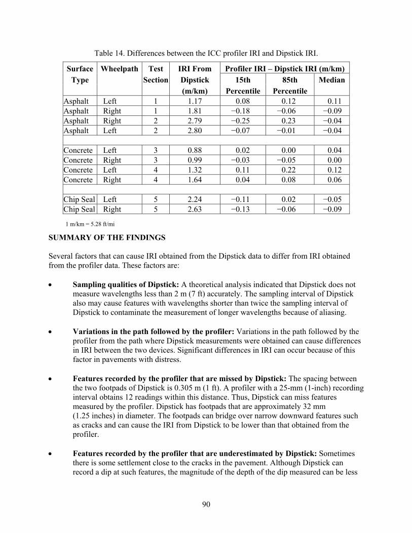
Table 14. Differences between the ICC profiler IRI and Dipstick IRI.

Surface Wheelpath Test IRI From Profiler IRI – Dipstick IRI (m/km) Type Section Dipstick 15th 85th Median

(m/km) Percentile Percentile Asphalt Left 1 1.17 0.08 0.12 0.11 Asphalt Right 1 1.81 −0.18 −0.06 −0.09 Asphalt Right 2 2.79 −0.25 0.23 −0.04 Asphalt Left 2 2.80 −0.07 −0.01 −0.04 Concrete Left 3 0.88 0.02 0.00 0.04 Concrete Right 3 0.99 −0.03 −0.05 0.00 Concrete Left 4 1.32 0.11 0.22 0.12 Concrete Right 4 1.64 0.04 0.08 0.06 Chip Seal Left 5 2.24 −0.11 0.02 −0.05 Chip Seal Right 5 2.63 −0.13 − −0.06 0.09

SUMMARY OF THE FINDINGS Seve th n cause IR btained the Dipstick data to dif IRI obtained from er hese factors are: n ties of D tick: A theoretical analysis indicated that Dipstick does not

lengths less than 2 m (7 ft) accurately. The sampling interval of Dipstick

• tions in he pa ed by the profiler: ions in fol the

r from path ip urem bt u ces in IRI between the two devices. S dif RI ecause of this

in ents with distress. • res ed by th profiler are mis Dipstic spacin een

o f ds of Dips is 0.30 ft). A with a 25-mm (1-inch) recording l o s 12 readin within stance. Thus, Dipstick can miss featu

measured by the profiler. Dipstick has ately 32 mm c diameter. The footpads can bridge over narrow downward features such s an cause t IRI from stick to be lower than that obtained fr e .

ted by Dipstick: S s

ent close to the cracks in the pavement. Although Dipstick can record a dip at such features, the magnitude of the depth of the dip measured can be less

81 m/km = 5.2 ft/mi

ral factors at ca I o from fer from the profil data. T

Sampli g quali ips•measure wavealso may cause features with wavelengths shorter than twice the sampling interval of Dipstick to contaminate the measurement of longer wavelengths because of aliasing.

Variapr file

t th follow wh e D

Variat the path lowed by se di ereno the er stick meas

ignificantents were o

ferences in Iained can ca can occur b

ff

factor pavem

Featu record e that sed by k: The g betwthe twinterva

ootpabtain

tickgs

5 m (1this di

profilerres

footpads that are approxim(1.25 in hes) in as crack and c he Dip om thprofiler

Features recorded by the profiler that are underestima ometime•there is some settlem

90

than th sampling the deepest part of

• ging eff cts of da LTPP , profi obta

25 m (1-inc intervals e proc ng P ch 0-mminc ving aver onto th m (1-in ta and th tracts dam ch) interv s. The I ompute this av profile is an ial When Dipstick measurements a rmed, r s will b ned ac avement and not on this artificial profile.

• k errors: E easure can occur because of incorrect

s ecorded, alfunction of Dipstick, or data entry errors during data input u These er s can ca bias in the IRI computed from the Dipstick data.

• n proce es for ck data: LTPP program, IRI values are

d g the ProQ l softwa hen ProQual computes I valu the e data ar anipulated and filter re com the IRIis RI value btained oQua oadRu d that

g ProQual had a slight upward bias. This is attributed to the filtering that is fore ProQual computes the IRI.

ipstick IRI and the profiler IRI in both magnitude and atial d

Despite t good ag±10 inomparisons use the average profiler IRI obtained from five error-free runs for comparison with

Althouconsidedistress e an IRI difference of ±0.16 m/km (±10 inches/mi)

etween the profiler IRI and the Dipstick IRI to judge the accuracy of LTPP’s profilers. If feren

necessa

at recorded by the profilers because the profilers have a much smaller interval and, thus, can capture the dip.

Avera e profiler ta: In the program le data ined at -m h) ar essed usi roQual, whi applies a 30

(11.8- h) mo age e 25-m ch) da en ex ta at 150-m (5.9-in al RI is c d using eraged , whichartific profile. re perfo eading e obtaion the tual p

Dipstic data rrors in Dipstick m mentsreading being r

. a m

to comp te IRI ror use a

IRI computatio d ru Di stip In thecompute usin ua re. W the IR es fromDipstickCompar

data, thon of I

e ms o

ed befol and R

puting f showe

. the IRI from Pr

computed usinperformed on the Dipstick data be

It is possible to have good agreement between profiler IRI and Dipstick IRI because the various errors compensate for each other. The cross-correlation technique can be used to determine whether there is agreement between the Dsp istribution.

all of these limitations with Dipstick, data from past LTPP comparisons have shown thareement between profiler IRI and Dipstick IRI, typically within ±0.16 m/km

ches/mi), can be obtained at many sections. Current procedures for LTPP profiler (cthe Dipstick IRI. This procedure helps to smooth out some of the variability in the profiler runs.

gh Dipstick can be used to check the IRI obtained from the profilers, it cannot be red for checking the accuracy of profilers on pavements that have rough features or . The current LTPP comparisons us

bdif ces outside of this limit are obtained on pavements having distress, it does not

rily mean that there is a problem with the profiler.

91

CHAPTER 7: OTHER FINDINGS FROM ANALYSIS OF THE DATA

INTRODUCTION This chapter describes other findings that were observed during the analyses that were performed for this research project. The specific findings that are described in this chapter are: • IRI values computed using ProQual. • Accelerometer effects on the T-6600 profiler data. • Observations on short-wavelength data collected by the T-6600 profiler. • IRI differences for the Southern profiler during the 1991 comparison. IRI VALUES COMPUTED USING PROQUAL The IRI values in the LTPP database have been computed using ProQual. The data collected by the DNC 690 profiler were at 152.4-mm (6-inch) intervals, and the IRI was computed using the collected data. Data at 25-mm (1-inch) intervals were available for the T-6600 and ICC profilers. ProQual applies a 300-mm (11.8-inch) moving average onto this data, extracts the data at 150-mm (5.9-inch) intervals, then computes the IRI using this data. The IRI computation algorithm contained in ProQual is the algorithm that is described in World Bank Technical Report 46.(9) This report indicates that the IRI algorithm will apply a 250-mm (9.8-inch) moving average onto the profile data before computing the IRI when the data recording interval is less than 250 mm (9.8 inches). Subsequent literature on IRI have indicated that the moving average applied by the IRI algorithm should be omitted if a moving average has already been applied to the profile data.(2,30) The World Bank report did not specifically describe such a criterion. A study was conducted to compare the IRI values computed using ProQual with those computed using RoadRuf. In this study, RoadRuf was used for computing the IRI with and without the moving average being enabled in the IRI algorithm. The five profile runs collected by the North Atlantic ICC profiler at the test site used in the 2003 LTPP profiler comparison were used for this study. The profile data used for this study were the ProQual-processed data, which were at 150-mm (5.9-inch) intervals. The average IRI values computed from the five runs for each wheelpath at all five sites are presented in table 15. There was excellent agreement among IRI values computed using ProQual and RoadRuf when the moving average was applied by the IRI algorithm in RoadRuf. (Note: The IRI algorithm automatically applies the moving average.) However, the IRI values computed using RoadRuf with the moving average omitted were slightly higher than those computed using ProQual. The IRI for the individual wheelpaths considered in this study ranged from 0.92 to 2.81 m/km (58 to 178 inches/mi), and the percent difference between IRI from ProQual and IRI from RoadRuf with the moving average omitted in the IRI algorithm ranged from 0.7 to 2.3 percent. A researcher who obtains 150-mm (5.9-inch) interval profile data from the LTPP database and

93

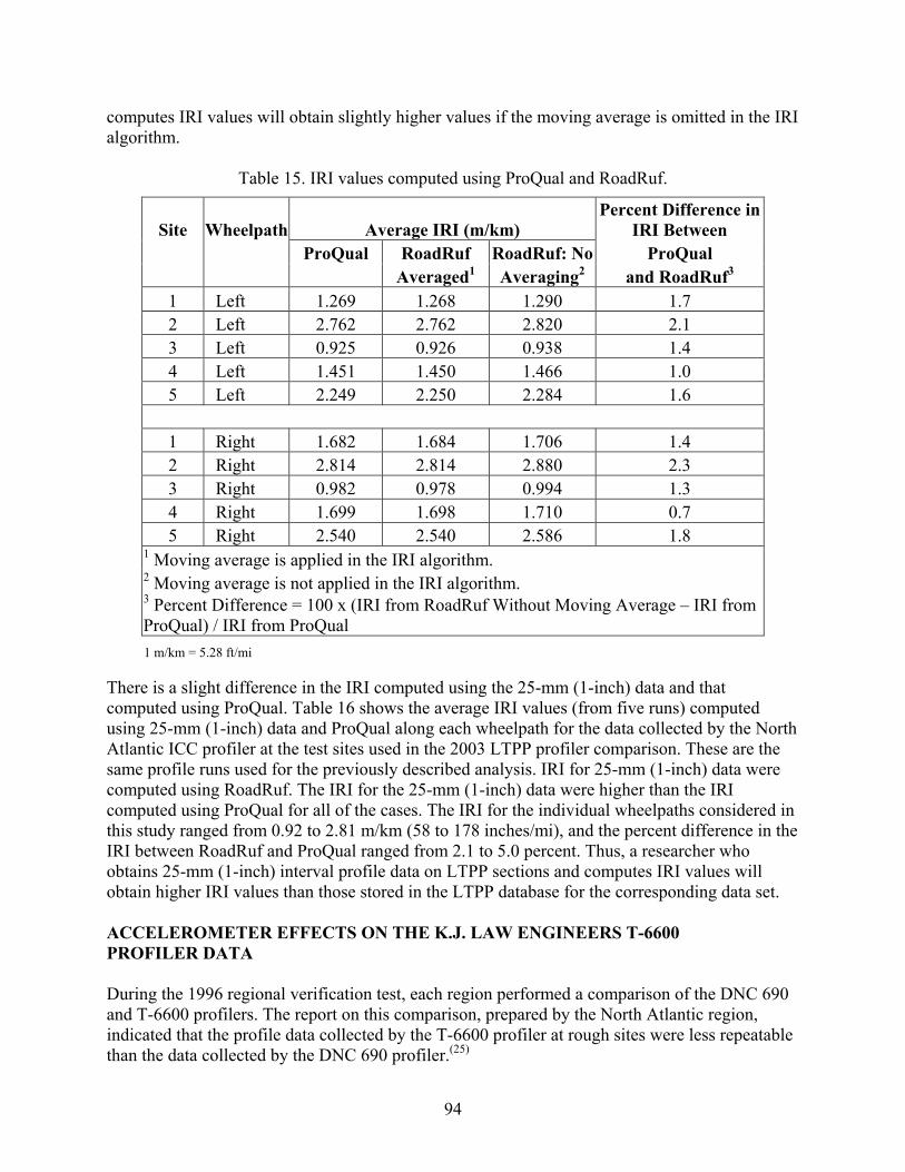
computes IRI values will obtain slightly higher values if the moving average is omitted in the IRI algo

I values computed using ProQual and RoadRuf.

Percent Difference in

rithm.

Table 15. IR

Site Wheelpath Average IRI (m/km) IRI Between ProQual RoadRuf RoadRuf: No ProQual Averaged1 Averaging2 and RoadRuf3

1 Left 1.269 1.268 1.290 1.7 2 Left 2.762 2.762 2.820 2.1 3 Left 0.925 0.926 0.938 1.4 4 Left 1.451 1.450 1.466 1.0 5 Left 2.249 2.250 2.284 1.6

1 Right 1.682 1.684 1.706 1.4 2 Right 2.814 2.814 2.880 2.3 3 Right 0.982 0.978 0.994 1.3 4 Right 1.699 1.698 1.710 0.7 5 Right 2.540 2.540 2.586 1.8

1 Moving average is applied in the IRI algorithm. 2 Moving average is not applied in the IRI algorithm. 3 Percent Difference = 100 x (IRI from RoadRuf Without Moving Average – IRI froProQual) / IRI from ProQual

m

There is a slight d

1 m/km = 5.28 ft/mi

ifference in the IRI computed using the 25-mm (1-inch) data and that omputed using ProQual. Table 16 shows the average IRI values (from five runs) computed

e

in the

to 5.0 percent. Thus, a researcher who btains 25-mm (1-inch) interval profile data on LTPP sections and computes IRI values will

0 n,

ble than the data collected by the DNC 690 profiler.

cusing 25-mm (1-inch) data and ProQual along each wheelpath for the data collected by the North Atlantic ICC profiler at the test sites used in the 2003 LTPP profiler comparison. These are thsame profile runs used for the previously described analysis. IRI for 25-mm (1-inch) data were computed using RoadRuf. The IRI for the 25-mm (1-inch) data were higher than the IRI computed using ProQual for all of the cases. The IRI for the individual wheelpaths considered inthis study ranged from 0.92 to 2.81 m/km (58 to 178 inches/mi), and the percent difference IRI between RoadRuf and ProQual ranged from 2.1 oobtain higher IRI values than those stored in the LTPP database for the corresponding data set. ACCELEROMETER EFFECTS ON THE K.J. LAW ENGINEERS T-6600 PROFILER DATA During the 1996 regional verification test, each region performed a comparison of the DNC 69and T-6600 profilers. The report on this comparison, prepared by the North Atlantic regioindicated that the profile data collected by the T-6600 profiler at rough sites were less repeata

(25)

94

Table 16. Comparison of the IRI from the 25-mm (1-inch) data with the IRI from ProQual.

SPercent

ce ite Wheelpath Average IRI (m/km) Differen ProQual 25-mm Data in IRI1

1 Left .32 1.27 1 3.9 2 Left 2.76 2.89 4.7 3 Left 0.92 0.95 3.3 4 Left 1.45 1.48 2.1 5 L 3.6 eft 2.25 2.33

1 R 3.6 ight 1.68 1.74 2 R 5.0 ight 2.81 2.95 3 Right 0.98 1.01 3.1 4 R 1.8 ight 1.70 1.73 5 R 3.9 ight 2.54 2.64

1 P l IRI)/ProQual IRI Percent Difference = 100 x (25-mm IRI – roQua Figure 68 shows the overlaid repeat r profile data collected by the North ite (section 4) during the regional verif n in this figure. The data show excel

laid right-sensor profiles of the K.J. Law Engineers DNC 690 profiler.

ft/m1 m/km = 5.28 i

profile plots of the right-senso Atlantic DNC 690 profiler at the rough concrete s

ication test. Profile data collected for five runs are showlent repeatability.

25.4 mm = 1 inch 1 m = 3.28 ft

15

-20

-15

-10

-5

0

5

10

0 25 50 75 100 125 150Distance (m)

Ele

vatio

n (m

m)

Figure 68. Over Figure 69 shows the overlaid repeat profile plots of the right-sensor profile data collected by the T-6000 profiler at the same site. This figure also contains data collected for five profile runs. The

95

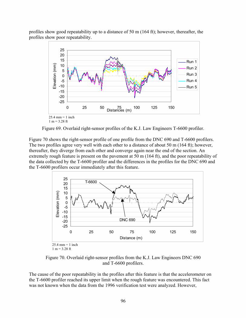
proprofiles show poor repeatability.

Figure ofiler.

igure 70 show or profile of one profile from the DNC 690 and T-6600 profilers.

ty of and

r immediately after this feature.

was not known when the data from the 1996 verification test were analyzed. However,

files show good repeatability up to a distance of 50 m (164 ft); however, thereafter, the

-25-20-15-10-505

10152025

Run 1

69. Overlaid right-sensor profiles of the K.J. Law Engineers T-6600 pr FT

s the right-senshe two profiles agree very well with each other to a distance of about 50 m (164 ft); however,

thereafter, they diverge from each other and converge again near the end of the section. An extremely rough feature is present on the pavement at 50 m (164 ft), and the poor repeatabilithe data collected by the T-6600 profiler and the differences in the profiles for the DNC 690 he T-6600 profilers occut

Figure 70. Overlaid right-sensor profiles from the K.J. Law Engineers DNC 690 and T-6600 profilers.

The cause of the poor repeatability in the profiles after this feature is that the accelerometer on the T-6600 profiler reached its upper limit when the rough feature was encountered. This fact

0 25 50 100 25 150Dis m)

Ele

vatio

n (m

m)

Run 2Run 3Run 4Run 5

75 1tances (

-25-20-15-10-505

10152025

0 25 50 75 100 125Distance (m)

Ele

vatio

n (m

m)

150

25.4 mm = ch 1 m = 3.28

25.4 mm = 1 inch 1 m

1 in ft

T-6600

DNC 690

= 3.28 ft

96

subsequent discussions with K.J. Law Engineers indicated that this indeed was the cause ofpoor profile repeatability. Since th

the e sensors on the DNC 690 profiler are housed on the vehicle

ody between the two axles, the accelerometers on the DNC 690 profiler are subjected to much ss acceleration than that felt by the accelerometers on the T-6600 profiler, which are housed in e sensor bar located on the front of the vehicle.

he IRI values for the five profiles shown in figure 68 for the DNC 690 profiler ranged from .82 to 1.90 m/km (115 to 120 inches/mi). The IRI values for the five profiles shown in figure 69 r the T-6600 profiler ranged from 1.87 to 1.91 m/km (119 to 121 inches/mi). The IRI for the o profiles shown in figure 70 were 1.85 m/km (117 inches/mi) for the DNC 690 profiler and

.87 m/km (119 inches/mi) for the T-6600 profiler. Although there was poor repeatability of the rofile data collected by the T-6600 profiler at this site, the IRI values for the five runs were milar. Also, the IRI values for the DNC 690 and T-6600 profilers were similar. Since IRI is rimarily influenced by wavelengths between 1 and 30 m (3 and 100 ft), the previously described bservations indicate that the poor repeatability of the profiles for the T-6600 profiler is caused y wavele an 30 m (100 ft).

The N d in e 19 test

com is maacceleromincreased from

collected by the Whree LTPP profilers.(14)

igure 71 shows an example of the data collected along the right wheelpath at section 2 by the Western sent in the Western profiler data, while thi r in the data collected by the North

entral profiler.

bleth T1fotw1psipob ngths greater th

orth Atlantic profiler encountered a similar situation at another rough site that was use96 regional verification test. However, this situation was not encountered at any of theth

sites that were used in the other three regions. It appears that when the T-6600 profiler encounters an extremely rough pavement feature, the accelerometer can go out of range, and thiscauses some contamination of the long-wavelength data that are collected after that event. However, this contamination appears to disappear after the profiler has traveled some distance after encountering the very rough spot.

“noisy” when compared to the data collected by the other t

In 2000, all four of LTPP’s profilers visited the K.J. Law Engineers facility in Michigan for puter maintenance and upgrades. The range of the accelerometers was increased during th

intenance by modifying the data collection software and by making modifications to the eter cards in the computer. After this upgrade, the range of the accelerometers

±2 gigabyte (GB) to ±8 GB, and the regional contractors indicated that they were able to obtain profiles that had better repeatability at rough sites.

OBSERVATIONS ON SHORT-WAVELENGTH DATA COLLECTED BY THE K.J. LAW ENGINEERS T-6600 PROFILERS

Data from the 2000 Profiler Comparison

The report prepared for the 2000 LTPP profiler comparison indicated that the profile data estern profiler at test sections 1 and 2, which were both AC pavements, were

F

and North Central profilers. The figure shows that a cyclic repetitive pattern is pres pattern does not occu

C

97

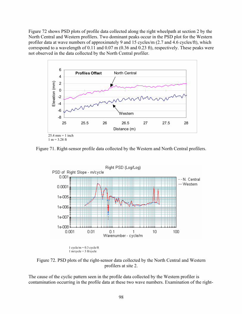
Figure 72 shows PSD plots of profile data collected along the right wheelpath at sectionNorth Central and Western profilers. Two dominant peaks occur in the PSD plot for the Westernprofiler data at wave numbers of approximately 9 and 15 cycles/m (2.7 and 4.6 cycles/ft), whichcorrespond to a wavelength of 0.11 and 0.07 m (0.36 and 0.23 ft), respectively. These peaks wernot observed in the data collected by the North Central profiler.

2 by the e

yclic pattern seen in the profile data collected by the Western profiler is contamination occurring in the profile data at these two wave numbers. Examination of the right-

Figure 71. Right-sensor profile data collected by the Western and North Central profilers.

-8

-6

-4

-2

0

2

4

6

Ele

vatio

n (m

m)

Figure 72. PSD plots of the right-sensor data collected by the North Central and Western profilers at site 2.

The cause of the c

25 25.5 26 26.5 27 27.5 28Distance (m)

Western

North CentralProfiles Offset

25.4 mm = 1 inch 1 m = 3.28 ft

1 cycle/m = 0.3 cycle/ft 1 m/cycle = 3 ft/cycle

98

wheelpath data collected at this site by the Western profiler using a PSD plot indicated that this

es/m (2.7 and 4.6 cycles/ft). For ll repeat runs along a specific path, the spikes in the PSD plots occurred at the same wave umbers.

n evaluation of the PSD plots of the profile data collected by the other three profilers at sites 1 nd 2 showed similar spikes in the PSD plots for the following cases:

Data collected by the North Atlantic profiler along both wheelpaths at sites 1 and 2.

Data collected by the North Central profiler along both wheelpaths at site 1, and along the left wheelpath at site 2.

Data collected by the Southern profiler along both wheelpaths at site 1.

or the North Atlantic profiler, two spikes in the PSD plot were similar to those seen for the estern p other two profilers, only a single spike was observed. For each profiler,

the wave n hich these spikes appeare e for both sites, and the spikes alsoiffagnitude of the spikes observed in the PSD plots was highest for the Western profiler. This

henomenon of spikes in the PSD plots for wave numbers greater than 1 cycle/m (0.3 cycle/ft) as not detected in the data collected by all of the profilers at the other three sites used in the 000 comparison.

he effects of the contamination were apparent in the Western profiler at sites 1 and 2, since the rofiles appeared to be noisy when compared to those obtained by the other three profilers. lthough evidence of contamination was not apparent in the data collected by the other profilers, e PSD plots indicated that the data were affected for several cases as described previously.

he cause of this contamination is not known. As this contamination was seen only at sites 1 and , it appears that an environmental condition during data collection, or some equipment factor, or

a combination of both, caused the contamination of the profile data. When the 25-mm (1-inch) profile data are proces ed using ProQual, the short wavelengths will become attenuated. Thus, the PSD plots of the 150-mm (5.9-inch) averaged data will not show spikes. The contamin le data occurs at very low wavelengths that are outside the wavelength range influencing the IRI. The IRI values computed for the Western profiler at sites 1 and 2 showed excellent agreem

phenomenon also was occurring along the right wheelpath. Evaluation of the data collected by the Western profiler at site 1 indicated that this phenomenon also was occurring along both wheelpaths. At sites 1 and 2, the two spikes in the left-sensor PSD plot occurred approximately at wave numbers of 5 and 14 cycles/m (1.5 and 4.3 cycles/ft), while for the right-sensor data, the spikes occurred approximately at wave numbers of 9 and 15 cyclan Aa • •

• FW rofiler. For the

umbers at w d were the sam appeared at the same wave numbers for the repeat runs. However, there were slight erences in the wave numbers at which the spikes appeared between the profilers. The d

mpw2 TpAth T2

s

ation of the profi

ent with the IRI values obtained for the other three profilers.

99

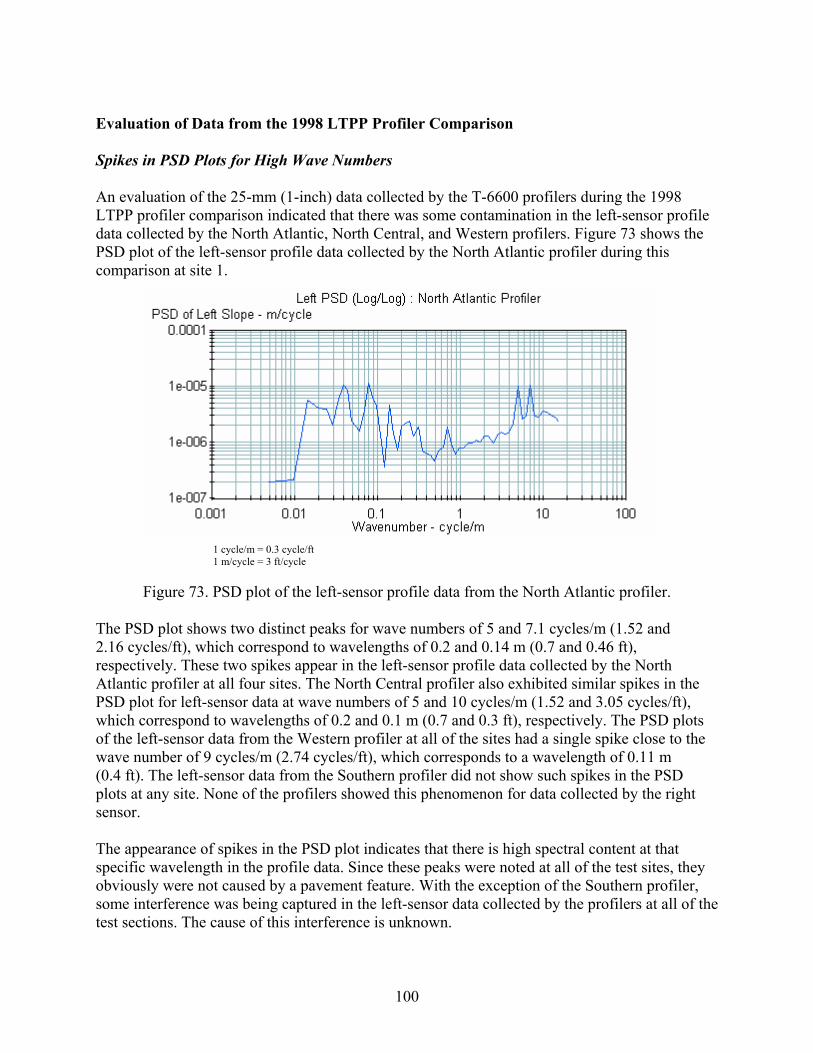
Evaluation of Data from the 1998 LTPP Profiler Comparison Spikes in PSD Plots for High Wave Numbers An evaluation of the 25-mm (1-inch) data collected by the T-6600 profilers during the 1998 LTPP profiler comparison indicated that there was some contamination in the left-sensor profile data collected by the North Atlantic, North Central, and Western profilers. Figure 73 shows the PSD plot of the left-sensor profile data collected by the North Atlantic profiler during this comparison at site 1.

ch correspond to wavelengths of 0.2 and 0.14 m (0.7 and 0.46 ft),

e

Figure 73. PSD plot of the left-sensor profile data from the North Atlantic profiler. The PSD plot shows two distinct peaks for wave numbers of 5 and 7.1 cycles/m (1.52 and 2.16 cycles/ft), whi

1 cycle/m = 0.3 cycle/ft 1 m/cycle = 3 ft/cycle

respectively. These two spikes appear in the left-sensor profile data collected by the North Atlantic profiler at all four sites. The North Central profiler also exhibited similar spikes in the PSD plot for left-sensor data at wave numbers of 5 and 10 cycles/m (1.52 and 3.05 cycles/ft), which correspond to wavelengths of 0.2 and 0.1 m (0.7 and 0.3 ft), respectively. The PSD plots of the left-sensor data from the Western profiler at all of the sites had a single spike close to thwave number of 9 cycles/m (2.74 cycles/ft), which corresponds to a wavelength of 0.11 m (0.4 ft). The left-sensor data from the Southern profiler did not show such spikes in the PSD plots at any site. None of the profilers showed this phenomenon for data collected by the right sensor. The appearance of spikes in the PSD plot indicates that there is high spectral content at that specific wavelength in the profile data. Since these peaks were noted at all of the test sites, they obviously were not caused by a pavement feature. With the exception of the Southern profiler, some interference was being captured in the left-sensor data collected by the profilers at all of thetest sections. The cause of this interference is unknown.

100

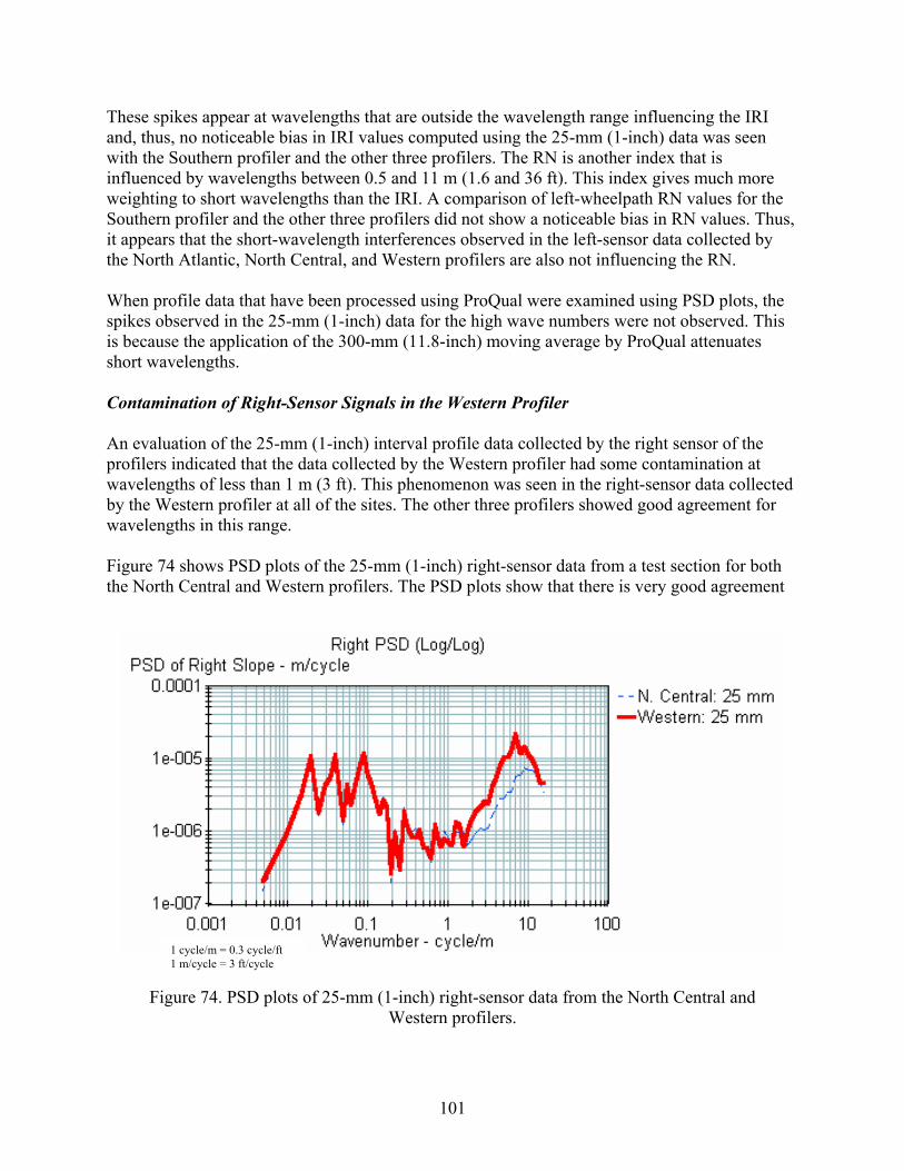
These spikes appear at wavelengths that are outside the wavelength range influencing the IRI m (1-inch) data was seen

ith the Southern profiler and the other three profilers. The RN is another index that is m (1.6 and 36 ft). This index gives much more

eighting to short wavelengths than the IRI. A comparison of left-wheelpath RN values for the hus,

have been processed using ProQual were examined using PSD plots, the ikes because the application of the 300-mm (11.8-inch) moving average by ProQual attenuates ort wavelengths.

ontamination of Right-Sensor Signals in the Western Profiler

n evaluation of the 25-mm (1-inch) interval profile data collected by the right sensor of the rofilers indicated that the data collected by the Western profiler had some contamination at avelengths of less than 1 m (3 ft). This phenomenon was seen in the right-sensor data collected y the Western profiler at all of the sites. The other three profilers showed good agreement for avelengths in this range.

igure 74 shows PSD plots of the 25-mm (1-inch) right-sensor data from a test section for both the North Central and Western profilers. The PS ots show that there is very good agreement

and, thus, no noticeable bias in IRI values computed using the 25-mwinfluenced by wavelengths between 0.5 and 11 wSouthern profiler and the other three profilers did not show a noticeable bias in RN values. Tit appears that the short-wavelength interferences observed in the left-sensor data collected by the North Atlantic, North Central, and Western profilers are also not influencing the RN. When profile data thatsp observed in the 25-mm (1-inch) data for the high wave numbers were not observed. This issh C Apwbw F

D pl

1 cycle/m = 0.3 cycle/ft 1 m/cycle = 3 ft/cycle

Figure 74. PSD plots of 25-mm (1-inch) right-sensor data from the North Central and Western profilers.

101

between the two profilers, except for the spectral content that has wave numbers greater than 1 cycle/m (0.3 cycle/ft), which corresponds to wavelengths of less than 1 m (3 ft). This phenomenon was observed for data collected by the Western profiler at all of the sites. Figure 75 shows the PSD plots for the ProQual-processed profile data for the two profile runs shown in figure 74. The application of the 300-mm (11.8-inch) moving average by ProQual attenuates profile features that have wave numbers greater than 1 cycle/m (0.3 cycle/ft), which orrespond to wavelengths of less than 1 m (3 ft). Thus, the difference between the two profilers

or een 1 and 0.03 cycle/m (0.3 and 0.009 cycle/ft), which correspond to

avelengths between 1 and 30 m (3 and 100 ft). This is the wavelength range that is primarily n the two profiles.

data indi values computed for the Western profiler were lower than the values obtainwavel

cfor wave numbers greater than 1 cycle/m (0.3 cycle/ft) that was seen in figure 74 is not noticeable in figure 75. The PSD plots for the two profilers shown in figure 75 agree fairly well for wave numbers greater than 1 cycle/m (0.3 cycle/ft). The plots show excellent agreement fwave numbers betwwinfluencing the IRI. Thus, there was good agreement in IRI betwee

1 cycle/m = 0.3 cycle/ft 1 m/cycle = 3 ft/cycle

Figure 75. PSD plots of ProQual-processed right-sensor data from the North Central and Western profilers.

The contamination of the right-sensor signal in the Western profiler occurs for short wavelengths that do not influence the IRI. Therefore, when an analysis of the IRI values from this comparison was performed, no bias in the IRI values for the Western profiler was seen. An evaluation of the RN values for the right-sensor data that were computed using the 25-mm (1-inch) interval profile

cated that the RNed for the other three profilers at all four of the test sites. This indicates that the short-ength contamination that is present in the Western profiler data is affecting the RN.

102

When overlaid left- and right-sensor data PSD plots of data collected by the Western profiler at

f the ata

ollected during the 2000 LTPP profiler comparison did not show such a trend. Therefore, it d

t

much higher that those computed from data collected by the other three profilers. The IRI values obtained for all four of the profilers for this comparison are presented in appendix A. The profile data collected by the Southern profiler at the eight test sections used in this comparison were compared to the data collected by the Western profiler to identify the cause of the high IRI values. An evaluation of the PSD plots of the Southern profiler data did not indicate any evidence of contamination at a specific wavelength. However, the PSD plots indicated that over a wavelength range of between 1 and 10 m (3 and 33 ft), the left-sensor data collected by the Southern profiler had slightly more spectral content than the data collected by the Western profiler. The cause of this phenomenon is unknown. This phenomenon resulted in higher IRI values being computed for the data collected by the left sensor in the Southern profiler. A comparison of the profile data collected by the two profilers using filtering techniques did not show the cause of the high IRI values of the left-sensor data from the Southern profiler. The data collected by the Southern profiler during the 1992 comparison did not show this phenomenon. SUMMARY OF THE FINDINGS ProQual applies a 300-mm (11.8-inch) moving average onto the 25-mm (1-inch) profile data collected by the T-6600 and ICC profilers and extracts the data points at 150-mm (5.9-inch)

tervals. The IRI values are computed using this averaged data. ProQual does not apply a

are a uses the IR ented in the World Bank report.(9) The

cally

ll be ightly higher than the IRI values for the corresponding section in the LTPP database.

the test sections were evaluated, the difference between the two sensors for wave numbers greater than 1 cycle/m (0.3 cycle/ft) was seen at all four of the test sites. An evaluation odata collected by the Western profiler during the 1996 regional verification test and the dcappears that this problem in the right sensor occurred at some point between 1996 and 1998, anwas fixed at some point between 1998 and 2000. This also could have been an intermittent problem with the sensor that occurred when testing was performed for the 1998 profiler comparison. IRI DIFFERENCES FOR THE SOUTHERN PROFILER DURING THE 1991 PROFILER COMPARISON The report prepared for the LTPP profiler comparison that was conducted in 1991 indicated thathe data collected by the left sensor in the Southern profiler was giving IRI values that were

(11)

inmoving average before computing the IRI for the data collected by the DNC 690 profiler, which

t 152.4-mm (6-inch) intervals, with a moving average having already been applied to thisI algorithm documdata by the profiler. ProQual

IRI algorithm applies a 250-mm (9.8-inch) moving average onto the profile data before computing IRI if the data recording interval is less than 250 mm (9.8 inches). Literature published after this report have indicated that the moving average applied by the IRI algorithm should be omitted if the profile data have already been subjected to a moving average.(2,30) However, the IRI values that are currently in the LTPP database have been computed by subjecting the profile data to two moving averages, one applied by ProQual and the other appliedby the IRI algorithm. If a researcher obtains profile data from the LTPP database and specifiomits the moving average that is applied by the IRI algorithm, the computed IRI values wisl

103

If a researcher obtains 25-mm (1-inch) interval LTPP profile data and computes the IRI, theresulting IRI values will be slightly higher than the corresponding IRI values that are in the LTPP database. This is because the IRI in the LTPP database have been computed after the 25-mm (1-inch) profile data have been processed using ProQual, which applies a 300-mm (11.8-inch) moving average onto the 25-mm (1-inch) data, extracts data at 150-mm (5.9-inch) intervals, and then uses that data to compute IRI. The profile da

ta for the repeat runs conducted by the T-6600 profiler before June 2000 may show oor repeatability at sections where an extremely rough localized feature is present on the

celerometer(s) in er range and contaminate the long wavelengths after that

vent. This occurrence will not affect the IRI computed from the profiles, since the contaminated

ta

tion in

urs

he 1998 LTPP profiler comparison indicated that some ontamination was present in the data collected by the right sensor of the Western profiler at

han

es

. nd was

ssed

on the

ppavement. This is because an extremely rough localized feature can cause the acthe profiler to exceed the accelerometewavelengths are outside of the wavelength range influencing the IRI. The range of the accelerometers in LTPP’s T-6600 profilers was increased during May–June 2000, and the dacollected after that were not expected to show such behavior. In some instances, PSD plots of data collected by T-6600 profilers showed either one or two spikes for wave numbers greater than 5 cycles/m (1.52 cycles/ft), which corresponds to wavelengths of less than 0.2 m (0.7 ft). This is an indication that there is some contaminathe profile data in the short wavelengths. This phenomenon will not be seen in the profile data that is in the LTPP database, since wavelengths of less than 1 m (3 ft) have been attenuated inthese profiles by the application of the moving average by ProQual. The cause of this contamination is not known. This contamination affects neither the IRI or the RN, since it occat wavelengths outside of the wavelength range influencing these two smoothness indices. Currently in the LTPP program, quality control of the profile data is performed using the ProQual-processed data. To detect contamination such as this, quality control procedures must be performed on the 25-mm (1-inch) data. An analysis of the data collected for tcwave numbers greater than 1 cycle/m (0.3 cycle/ft), which corresponded to wavelengths less t1 m (3 ft). This phenomenon will not be seen in the ProQual-processed data, since short wavelengths are attenuated by the application of the moving average. The contamination donot affect the IRI because it occurs at wavelengths that are outside of the range of the wavelengths influencing the IRI. However, it is affecting the RN computed from the 25-mm (1-inch) data. This phenomenon was not noted in the data collected by the Western profiler during the 1996 verification study nor in the data collected during the 2000 profiler comparisonTherefore, it appears that this phenomenon occurred sometime between 1996 and 1998, afixed sometime between 1998 and 2000, or perhaps this is an intermittent problem. Currently, inthe LTPP program, quality control of the profile data is performed using the ProQual-procedata. To detect contamination such as this, quality control procedures must be performed 25-mm (1-inch) data.

104

CHAPTER 8: CONCLUSIONS AND RECOMMENDATIONS

High-quality longitudinal profile data have been collected with all three inertial profilers thhave been used in the LTPP program—the DNC 690, T-6600, and ICC profilers. The data collected by these profilers provide a valuable reso

at

urce for researchers. Good agreement in IRI alues between the DNC 690 and T-6600 profilers was observed. Also, good agreement in IRI

t any

es n error,

(0.4

e ctual

FFECT OF APPLYING A MOVING AVERAGE ONTO PROFILE DATA

CC

ervals.

tes e

e

or for those who are interested in examining minute details in the profile .g., pavement distresses and joints in PCC pavements). Therefore, it is recommended that a

rocedure be put in place where the 25-mm (1-inch) interval data are easily available to researchers.

vvalues between the T-6600 and ICC profilers was observed. This indicates that the IRI values in the LTPP database can be used for analysis of roughness progression at test sections withouadjustments being made to the IRI values obtained by the different profilers. The research also indicated that using IRI to evaluate profiler repeatability, accuracy, and reproducibility is not sufficient. The following are conclusions and recommendations based on the analyses that were conducted for this project. DATA COLLECTED BY INERTIAL PROFILERS Conclusions: Data collected by inertial profilers do not accurately portray very narrow featursuch as cracks in either AC or PCC pavements, or joints in PCC pavements. This is not abut rather an effect of the low-pass filtering that is performed on the profile data. Evaluation of 25-mm (1-inch) data collected by both the T-6600 and ICC profilers over a joint in a PCC pavement showed that the joint appeared in the profile as a feature that was spread over a distance of 75 mm (3 inches), when the width of the joint was actually closer to 10 mminches). This happens because of the low-pass filter that is applied to the profile data. The low-pass filter applied to the profile data will distort narrow downward features by attenuating thdepth of the feature, and will also spread the feature over a distance that is more than the awidth of the feature. E Conclusions: In the LTPP program, the 25-mm (1-inch) data obtained from the T-6600 and Iprofilers are processed using the ProQual software. ProQual applies a 300-mm (11.8-inch) moving average onto the 25-mm (1-inch) data and extracts data at 150-mm (5.9-inch) intThese data are used to compute IRI values, and this averaged data are uploaded to the LTPP database. The application of the moving average onto the 25-mm (1-inch) data attenuafeatures with wavelengths less than 1 m (3 ft). Detailed profile features cannot be observed in thProQual-processed data because of this effect. The moving average also can cause distortion of the profile data, and the averaged data can show features that are not actually present in thpavement while eliminating features that are present. Recommendations: Although the profile data that are currently in the LTPP database can be used for many research purposes, these data are not useful for researchers who are interested in short-wavelength data (ep

105

COMPA ERS Conclusions: Since the DNC 690 profiler recorded profile data at 152.4-mm (6-inch) intervals,

0

OMPARISON OF THE K.J. LAW ENGINEERS T-6600 AND ICC PROFILERS

onclusions: Since the 25-mm (1-inch) interval data were available for both the T-6600 and

tent

ed by the two profilers, although both profilers apply an upper-wavelength utoff filter of 100 m (328 ft). When the ProQual-processed data for the two profilers are

een, and good greement between the two profilers will be seen for wavelengths less than 1 m (3 ft) since the

a before computing IRI if the data cording interval is less than 250 mm (9.8 inches). Literature published after the World Bank

if

has d to a 304.8-mm (12-inch) moving average. When ProQual computes IRI from

RISON OF THE K.J. LAW ENGINEERS DNC 690 AND T-6600 PROFIL

when comparing data from the T-6600 profiler with the DNC 690 profiler, only the 150-mm (5.9-inch) interval ProQual-processed data from the T-6600 profiler can be compared. Comparison of profile data for the two profilers showed good agreement, although there were some differences in the profiles for sections that had significant long-wavelength content. Thesedifferences are attributed to the different long-wavelength cutoff filter values used with the two profilers (91 m (300 ft) for the DNC 690 profiler, and 100 m (328 ft) for the T-6600 profiler). An evaluation of the profile data indicated that the long-wavelength cutoff filtering technique used in both of these profilers appeared to be similar. Good agreement in IRI values for the DNC 69and T-6600 profilers was observed. C CICC profilers, a comparison of the 25-mm (1-inch) interval data for the two profilers could be performed. Comparison of profile data for the two profilers using PSD plots indicated that there were differences in both the short and long wavelengths. There was good agreement in the profile data for the two profilers for wavelengths between 1 and 40 m (3 and 131 ft). For wavelengths less than 1 m (3 ft), the ICC profiler usually showed a higher wavelength conthan the T-6600 profiler. This is attributed to the smaller footprint of the ICC profiler, which most likely caused texture effects and the higher magnitude of narrow features to be recorded. For wavelengths greater than 40 m (131 ft), the T-6600 profiler recorded more wavelength content than the ICC profiler. This is attributed to differences in the long-wavelength filtering techniques that are usccompared using PSD plots, only the differences at the higher wavelengths will be saapplication of the moving average attenuates the short-wavelength features. Good agreement in IRI, which is primarily influenced by wavelengths between 1 and 30 m (3 and 100 ft), was obtained for data collected by these two profilers. IRI VALUES Conclusions: In the LTPP program, IRI values are computed using ProQual, which uses the IRIalgorithm documented in World Bank Technical Report 46.(9) The IRI algorithm applies a 250-mm (9.8-inch) moving average onto the profile datrereport have indicated that the moving average applied by the IRI algorithm should be omitted the profile data have already been subjected to a moving average.(2,30) Before computing IRI, ProQual applies a 300-mm (11.8-inch) moving average onto the 25-mm (1-inch) profile data collected by the T-6600 and ICC profilers; however, this moving average is not applied to the 152.4-mm (6-inch) interval profile data collected by the DNC 690 profiler, which alreadybeen subjecte

106

such data, the moving average in the IRI algorithm is applied to the data. Thus, during

roQual and the other applied by the IRI algorithm. This will cause a slight downward bias in the

rvals and uses these data to compute IRI.

nderestimates the IRI value. The procedure described in the World Bank report on which the

sing ge

g

Variations in the path followed by the profiler from the path where Dipstick ments are performed.

Features recorded by the profiler that are missed by Dipstick.

d

computation of IRI, the profile data are subjected to two moving averages, one applied by PIRI values. A limited analysis using a set of sections with IRI ranging from 0.9 to 2.8 m/km (57 to 178 inches/mi) showed that the current LTPP procedures for computing IRI result in a downward bias in IRI ranging from 0.7 to 2.3 percent. The IRI is influenced by the sampling interval. Thus, if a researcher obtains 25-mm (1-inch) interval LTPP profile data and computes IRI, the resulting IRI values will be slightly higher thanthe corresponding IRI values that are stored in the LTPP database. This is because IRI in the LTPP database have been computed after the 25-mm (1-inch) profile data have been processed using ProQual, which applies a 300-mm (11.8-inch) moving average onto the data, then extracts data points at 150-mm (5.9-inch) inte Recommendations: The current procedure used by ProQual to compute IRI slightly uIRI computation procedure used in ProQual is based does not specifically indicate that the moving average applied by the IRI algorithm should be omitted if the profile data have alreadybeen subjected to a moving average.(9) Since all time-sequence IRI values for a test section have this bias, the bias in the IRI values will not affect roughness progression studies performed uthese data. Reprocessing profile data to compute IRI values by omitting the moving averaapplied by the IRI algorithm will be a major undertaking that will require a vast amount of resources. The very slight bias in IRI is not a major error that justifies reprocessing the IRI values. Thus, it is recommended that no changes be made to the current procedure for computinIRI values. DIFFERENCES IN IRI BETWEEN PROFILERS AND DIPSTICK Conclusions: A variety of factors can cause the IRI obtained from the Dipstick data to differ from the IRI obtained from the profiler data. The factors that contribute to the differences between the Dipstick IRI and the profiler IRI are: • Sampling qualities of Dipstick. •

measure•• The footpads of Dipstick bridging over narrow downward features that are measured by

the profiler. • Features recorded by the profiler that are underestimated by Dipstick because the footpa

of Dipstick may not rest in the deepest part of a feature. • Differences between the profiles used for computing the difference in IRI between

profilers and Dipstick because of the application of the moving average onto profiler data.

• Errors in Dipstick measurements. • IRI computational procedure for Dipstick data used in the ProQual software.

107

Despite these limitations, data from past LTPP comparisons have shown that good agrebetween profiler IRI and Dipstick IRI, typically within ±0.16 m/km (±10 inches/mi), can usbe obtained at sections that do not have significant distress. Current procedures for LTPP profiler comparisons use the average profiler IRI obtained from five error-free runs for comparison wthe Dipstick IRI. This procedure helps smooth out some of the variability in the profiler runs.

ement ually

ith

ecommendations: One of the tasks in this project was to provide recommendations on I

onclusions: The profile data for repeat runs that were collected by the T-6600 profiler before calized

)

pikes in PSD Plots

onclusions: In some instances, PSD plots of data collected by T-6600 profilers showed either s

he he profile data that are in the LTPP database,

nce wavelengths of less than 1 m (3 ft) have been attenuated in these profiles by applying the mination is not known. This contamination does not

e influen presence of this contamination will not affect many of the

Recom Researchers who are using the 25-mm (1-inch) data and performing

ould n to

with

Rrecalculating IRI because of differences between profiler IRI and Dipstick IRI. The current IRvalues in the LTPP database that were computed from profiler data are considered to be accurate, and no recalculation of IRI is necessary. REPEATABILITY OF THE K.J. LAW ENGINEERS T-6600 PROFILER CJune 2000 may show poor repeatability at a few sections where an extremely rough lofeature is present on the pavement. This is because such a feature can cause the accelerometer(sin the profiler to exceed the range and contaminate the long wavelengths in the profile data collected after such an event. However, IRI computed from such profiles still will be accurate, since the contaminated wavelengths are outside of the wavelength range influencing the IRI. The range of the accelerometers in LTPP’s T-6600 profilers was increased during May–June 2000, and data collected after that were not expected to show such behavior. SHORT-WAVELENGTH ERRORS IN DATA COLLECTED BY THE K.J. LAW ENGINEERS T-6600 PROFILER S Cone or two spikes for wave numbers greater than 5 cycles/m (1.52 cycles/ft), which correspondto wavelengths less than 0.2 m (0.7 ft). This indicates that there is some contamination in tprofile data. This phenomenon will not be seen in tsimoving average. The cause of this contaaffect the IRI or RN because it occurs at wavelengths outside of the wavelength rang

cing both of these indices. The analyses that can be performed using the 25-mm (1-inch) profile data.

mendations:research that make use of the extremely short wavelengths should be aware of this issue. They sh evaluate the data and determine whether any contamination is present in the short wavelengths and, if it is present, determine whether it will impact the research that they plado that data.

108

Western K.J. Law Engineers T-6600 Profiler Data Conclusions: Data obtained from the 1998 LTPP profiler comparison indicated that some contamination was present in the data collected by the right sensor of the Western profiler for wave numbers greater than 1 cycle/m (0.3 cycle/ft), which corresponds to wavelengths less than

d to the .

However, the contamination is affecting the RN omputed from 25-mm (1-inch) data. The presence of this contamination does not mean that the

(1-inch) data ith this contamination cannot be used for any analyses that make use of wavelengths of less

n.

o as fixed, and to identify

e cause of the problem. Overlaid PSD plots of left- and right-sensor data for the set of profiles ct

should be aware of this issue, since this contamination can e interpreted as a pavement effect.

ECOMMENDATIONS FOR IMPROVING CURRENT LTPP DATA COLLECTION

data

s can cancel out errors. In the field during data collection, particular attention should be paid before recording high

m repeat runs to evaluate the repeatability of the data, (2) overlay of the data collected during the current data collection with the data collected during the previous visit to the site to determine whether or not they agree, (3) verification that spikes noted in the profile are caused by pavement features and not by any other factor, (4) evaluation of the repeatability of the IRI values, and (5) comparison of IRI obtained during the

1 m (3 ft). This phenomenon will not be seen for ProQual-processed data that are uploadeLTPP database, since short wavelengths are attenuated by the application of the moving averageThe contamination does not affect IRI because it occurs at wavelengths that are outside of the range of wavelengths influencing the IRI. c25-mm (1-inch) data obtained from this sensor are not usable. However, 25-mm wthan 1 m (3 ft). This phenomenon was not noted in the data collected by the Western profiler during the 1996 verification study nor in the data collected during the 2000 profiler comparisoTherefore, it appears that this phenomenon occurred sometime between 1996 and 1998, and was fixed sometime between 1998 and 2000, or perhaps this is an intermittent problem. Recommendations: It is recommended that a set of 25-mm (1-inch) interval data collected by the Western profiler at regular time periods (e.g., 6-month intervals) be obtained and reviewed tpinpoint when the problem with the sensor began, when the problem wthcan be used to investigate this issue. Researchers who use 25-mm (1-inch) data and conduresearch involving short wavelengthsb RAND DATA PROCESSING PROCEDURES • The current field procedures for collecting profile data using inertial profilers are

considered to be adequate, and no changes to current procedures are required. • Errors during Dipstick data collection can occur because of data recording errors and

equipment problems. A closure error check is performed at the end of Dipstick collection as a quality control procedure. However, it still is possible to pass the closure error criterion even with erroneous data, as compensation effect

data values to ensure that such readings are indeed correct. • Currently, in the LTPP program, there are several procedures in place to ensure the

quality of the profile data.(6) These procedures include: (1) overlay of the profile data obtained fro

109

current data collection for each wheelpath with IRI obtained during the previous visit to ks are performed on the ProQual-

processed averaged data and will not detect problems that may occur in wavelengths less oving

n

rs

1 m (3 ft)), but yet the IRI values can show very good agreement because these short wavelengths do not influence the IRI. Thus, it is

h) d using PSD plots during future comparisons so

that the short-wavelength data collection capabilities of the profilers also can be

Although Dipstick can be used to check IRI obtained from the profilers, it cannot be used

s.

ormed to identify the cause of the difference in IRI.

•

the site. However, all these quality control chec

than 1 m (3 ft). These short wavelengths are attenuated when ProQual applies the maverage onto the profile data. Thus, short-wavelength data can be evaluated only by analyzing 25-mm (1-inch) data. It is possible to satisfy all the quality control checks that are currently performed on the LTPP data and yet have data errors in the short wavelengths. It is recommended that a quality control procedure be adopted to check the 25-mm (1-inch) data collected by the profilers. The recommended procedure is to obtaia set of data collected by each of LTPP’s profilers at regular intervals (e.g., 6-monthintervals) and compare the data with the data collected at the same sites during the previous visit to the site by using PSD plots. A consistent difference in the short wavelengths for the two data sets or any sharp spikes in the PSD plots for wave numbegreater than 1 cycle/m (0.3 cycle/ft) will indicate potential problems in the short-wavelength data collected by a profiler.

RECOMMENDATIONS ON LTPP PROFILER COMPARISONS • It is recommended that LTPP profiler comparisons be conducted at regular intervals to

compare the outputs obtained from the four profilers. The data obtained from such comparisons will verify whether all four of the profilers are collecting similar data.

• In the current profiler comparison procedures, emphasis is placed on comparing IRI.

However, there can be differences in the short-wavelength data collected by the profilers (i.e., for wavelengths less than

recommended that in addition to the current data analysis procedures, the 25-mm (1-incdata collected by the profilers be evaluate

compared.

•to check the accuracy of the profilers on pavements that have rough features or distresThe current LTPP comparisons use an IRI difference of ±0.16 m/km (±10 inches/mi)between the profiler IRI and Dipstick IRI to judge the accuracy of LTPP’s profilers. If differences outside of this limit are obtained on pavements with distress or on rough pavements, it does not necessarily mean that there is a problem with the profiler. If such occurrences are encountered, an investigation should be perf

Research performed for this project showed that agreement in IRI values at a section between the profilers can occur because the errors compensate for each other. Roughness profiles or cross correlations are techniques that can be used to compare spatial distribution of IRI within a section between the profilers. It is recommended that such procedures be used in addition to current procedures when analyzing data from LTPP comparison studies.

110

APPENDIX A: LTPP PROFILER COMPARISON STUDIES

OMPARISON: AUSTIN, TX

mparison was conducted in February 1990. The information presented in this section was d from a paper written about this comparison.

1990 C This coobtaine The fou m (1056 fwheelpruns at was marked s were asked to align the profiler along this

ath. Each test section was divided into two sections for analysis, resulting in the availability of re the main findings

om this study:

• for

wheelpath usually was higher than that for the left wheelpath. Poor agreement between

•

cases

a, which e of the high IRI value. It was concluded that the side-to-side rocking motion

induced on the profiler when traversing these rough sections caused sunlight to seep

•

•

o Left Wheelpath: Seven sections had IRI values between 1.2 and 2.4 m/km

m

ches/mi), five sections had IRI values between 2.4 and 4.7 m/km

(10)

r LTPP DNC 690 profilers were used in this comparison. Six test sections, each 322t) long were established for testing. Reference profile measurements along both aths at the test sections were obtained using Dipstick. The profilers performed five repeat each test section at speeds of 56 and 80 km/h (35 and 80 mi/h). The left wheelpath at the test sections and the profiler driver

p12 sections for comparing the profiler and Dipstick IRI. The following afr

In most cases, better agreement between profiler IRI and Dipstick IRI was obtainedthe left wheelpath than for the right wheelpath. It was noted that the IRI for the right

profiler IRI and Dipstick IRI usually occurred at the rough sections.

Significant differences between profiler IRI and Dipstick IRI were noted for several cases, with the profiler IRI being much higher than the Dipstick IRI. Most of thewhere these significant differences occurred were along the right wheelpath at extremely rough sections that had Dipstick IRI values in excess of 4 m/km (254 inches/mi). An evaluation of the profiler data for such cases indicated saturation spikes in the datwas the caus

under the shroud covering the sensors and contaminate the profile data.

Evaluation of the profiles also indicated instances where lost lock occurred. This was another factor contributing to differences between Dipstick and profiler IRI values.

An evaluation of the Dipstick IRI values obtained for the 12 sections indicated the following IRI distribution:

(76 and 152 inches/mi), three sections had IRI values between 2.4 and 4.7 m/k(152 and 298 inches/mi), and two sections had IRI values exceeding 4.7 m/km (298 inches/mi).

o Right Wheelpath: Five sections had IRI values between 1.2 and 2.4 m/km

(76 and 152 in

111

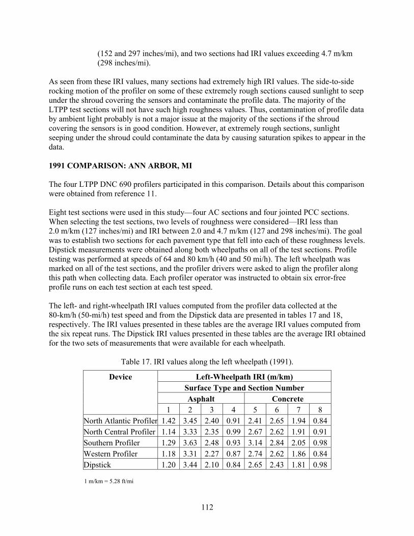
(152 and 297 inches/mi), and two sections had IRI values exceeding 4.7 m/km

As seen from these IRI values, many sections had extremely high IRI values. The side-to-side rocking motion of the profiler on some of these extremely rough sections caused sunlight to seep

d contaminate the profile data. The majority of the TPP test sections will not have such high roughness values. Thus, contamination of profile data

xtremely rough sections, sunlight eping under the shroud could contaminate the data by causing saturation spikes to appear in the

son

s were used in this study—four AC sections and four jointed PCC sections. hen selecting the test sections, two levels of roughness were considered—IRI less than m/k l

was to els. Dipstictesting t wheelpath was

arked on all of the test sections, and the profiler drivers were asked to align the profiler along s pat

profile The lef80-km/respectthe six ined for the

(298 inches/mi).

under the shroud covering the sensors anLby ambient light probably is not a major issue at the majority of the sections if the shroud covering the sensors is in good condition. However, at esedata. 1991 COMPARISON: ANN ARBOR, MI The four LTPP DNC 690 profilers participated in this comparison. Details about this compariwere obtained from reference 11. Eight test sectionW2.0 m (127 inches/mi) and IRI between 2.0 and 4.7 m/km (127 and 298 inches/mi). The goa

establish two sections for each pavement type that fell into each of these roughness levk measurements were obtained along both wheelpaths on all of the test sections. Profile was performed at speeds of 64 and 80 km/h (40 and 50 mi/h). The lef

mthi h when collecting data. Each profiler operator was instructed to obtain six error-free

runs on each test section at each test speed.

t- and right-wheelpath IRI values computed from the profiler data collected at the h (50-mi/h) test speed and from the Dipstick data are presented in tables 17 and 18, ively. The IRI values presented in these tables are the average IRI values computed from repeat runs. The Dipstick IRI values presented in these tables are the average IRI obtatwo sets of measurements that were available for each wheelpath.

Table 17. IRI values along the left wheelpath (1991).

Device Left-Wheelpath IRI (m/km) Surface Type and Section Number Asphalt Concrete

1 2 3 4 5 6 7 8 North Atlantic Profiler 1.42 3.45 2.40 0.91 2.41 2.65 1.94 0.84 North Central Profiler 1.14 3.33 2.35 0.99 2.67 2.62 1.91 0.91 Southern Profiler 1.29 3.63 2.48 0.93 3.14 2.84 2.05 0.98 Western Profiler 1.18 3.31 2.27 0.87 2.74 2.62 1.86 0.84 Dipstick 1.20 3.44 2.10 0.84 2.65 2.43 1.81 0.98

1 m/km = 5.28 ft/mi

112

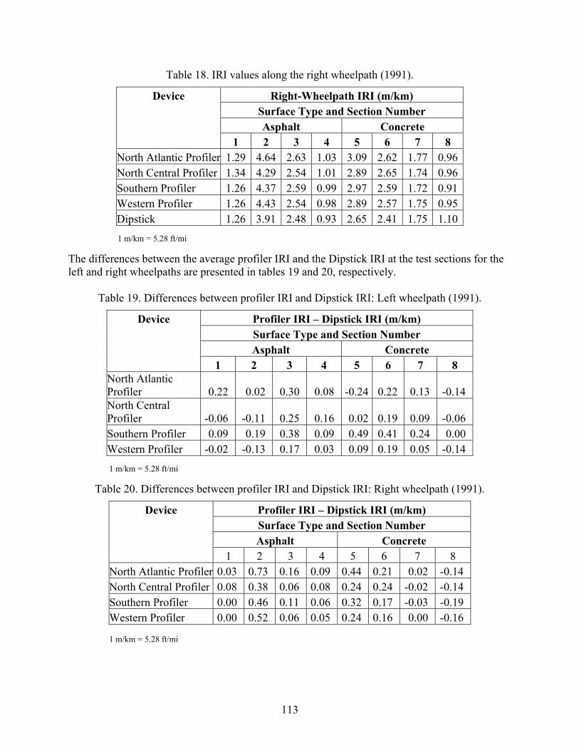
Table 18. IRI values along the right wheelpath (1991).

Device Right-Wheelpath IRI (m/km) Surface Type and Section Number Asphalt Concrete

1 2 3 4 5 6 7 8 North Atlantic Profiler 1.29 4.64 2.63 1.03 3.09 2.62 1.77 0.96 North Central Profiler 1.34 4.29 2.54 1.01 2.89 2.65 1.74 0.96 Southern Profiler 1.26 4.37 2.59 0.99 2.97 2.59 1.72 0.91 Western Profiler 1.26 4.43 2.54 0.98 2.89 2.57 1.75 0.95 Dipstick 1.26 3.91 2.48 0.93 2.65 2.41 1.75 1.10

nted in tables 19 and 20, respectively.

1 m/km = 5.28 ft/mi The differences between the average profiler IRI and the Dipstick IRI at the test sections for the left and right wheelpaths are prese

Table 19. Differences between profiler IRI and Dipstick IRI: Left wheelpath (1991).

Device Profiler IRI – Dipstick IRI (m/km) Surface Type and Section Number Asphalt Concrete

1 2 3 4 5 6 7 8 North Atlantic Profiler 0.22 0.02 0.30 0.08 -0.24 0.22 0.13 -0.14 North Central Profiler -0.06 -0.11 0.25 0.16 0.02 0.19 0.09 -0.06 Southern Profiler 0.09 0.19 0.38 0.09 0.49 0.41 0.24 0.00 Western Profiler -0.02 -0.13 0.17 0.03 0.09 0.19 0.05 -0.14

Table 20. Differences between profiler IRI and Dipstick IRI: Right wheelpath (1991).

1 m/km = 5.28 ft/mi

Devi ) ce Profiler IRI – Dipstick IRI (m/km Surface Type and Section Number Asphalt Concrete

1 2 4 5 8 3 6 7 North Atlant Profileic r 0.03 0.73 0.16 0.09 0.44 0.21 0.02 -0.14 North Central Profiler 0.08 0 0 0 0 0 -0.02 .38 .06 .08 .24 .24 -0.14S 0 0 0 0 0 outhern Profiler 0.00 .46 .11 .06 .32 .17 -0.03 -0.19W 0.00 0.52 0.06 0.05 0.24 0.16 estern Profiler 0.00 -0.16

1 m/km = 5.28 ft/mi

113

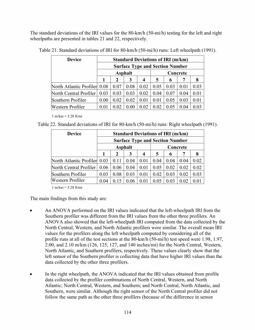
The standard deviatio r the left and right wheelpaths are presented in tables 21 and 22, respectively.

Table . Standard deviations of IRI lpath (1991).

Device Standard Deviations of IRI (m/km)

ns of the IRI values for the 80-km/h (50-mi/h) testing fo

21 for 80-km/h (50-mi/h) runs: Left whee

Surfa p o mce Ty e and Secti n Nu ber Asph calt Con rete

1 2 3 4 5 6 7 8 North Atlantic Profiler 0.08 0.07 0.08 0.02 0.05 0.03 0.01 0.03 North Central Profiler 0.03 0.03 0.03 0.02 0.04 0.07 0.04 0.01 Southern Profiler 0.00 0.02 0.02 0.01 0.01 0.05 0.03 0.01 Western Profiler 0.01 0.02 0.00 0.02 0.02 0.05 0.04 0.03

1 m/km = 5.28 ft/mi

Table 22. Standard deviations of IRI for 80-km/h (50-mi/h) runs: Right wheelpath (1991).

Device Standard Deviations of IRI (m/km) Surface Type and Section Number Asphalt Concrete

1 2 3 4 5 6 7 8 North Atlantic Profiler 0.03 .11 4 0.01 0.04 0.04 0.04 0.02 0 0.0North Central Profiler 0.06 0.06 0.04 0.01 0.05 0.02 0.02 0.02 Southern Profiler 03 8 00. 0.0 0.03 0.01 0.02 0.03 0.02 .03 Western Profiler 0 5 00. 4 0.1 0.06 0.01 0.05 0.03 0.02 .01

The mai is s e

• An ANOVA performed on the IRI values indicated that the left-wheelpath IRI from the

ANOVA wed that the left collected by the N rth Ce stern, and North erall mean IRI values for the profilers along the l g all of the profile runs at all of the test sections at the 80-km/h (50-mi/h) test speed were 1.98, 1.97, 2.00, and 2.10 m/km (126, 5, 1 and 0 in es/m for t Nor entral, Western, N r c . c at the le i n a v han the d e e l

In th, th d h v o d rofile

d the profiler combinations of North Central, Western, and North Atlantic; North Central, Western, and Southern; and North Central, North Atlantic, and Southern, were similar. Although the right sensor of the North Central profiler did not follow the same path as the other three profilers (because of the difference in sensor

1 m/km = 5.28 ft/mi

n findings from th tudy ar :

Southern profiler was different from the IRI values from the other three profilers. An also shontral, We

-wheelpath IRI computed from the data Atlantic profilers were similar. The ovo

eft wheelpath computed by considerin

12 27, 14 ch i) he th Corth Atlantic, and Southern p ofilers, respe tively These values learly show thft sensor of the Souther

othn prof ler is collecti g data that h ve higher IRI alues t

ata collected by the r thre profi ers.

the right wheelpa e ANOVA indicate that t e IRI alues btaine from p•ata collected by

114

spacing), all three cases in which the profilers were not significant in the ANOVA involved this profiler. Although the North Atlantic, Western, and Southern profilers have similar sensor spacing, the ANOVA indicated that at least one of the profilers was

wheelpath d by consideri t sections at the 80-km/h (5 test speed wer , 137, 143, and 138 inches/mi) for the North Cent ern profilers, respectively. Although the ANOVA indicated that the IRI va four profilers were not similar, an examina n o e IR ilers the test sec i p l f a com

• The results of the ANOVA for the left-wheelpa I e t g

wa or the t lp h d s g nt factor for two of the profiler combinations out of a total of five combinations that were analyzed.

• All profile d excellent rep elpaths, except

at a ew se t had spikes i the repeatability of profilers was not affected b ), the level of rou ness, or the two speeds selec ting. Although th profiler was producing higher IRI values when compared to the other three profilers along the left wh R e ai y p r ble to tho e le

1992 COM S, IA

he four L rofilers participated in this comparison. The information presented in ent written about this comparison.(12)

ght te

(127 inestablisDipstic measurwere oblevel mone whmeasurequest d profile runs at a section for each test speed.

measur or determobtaine

different from the rest. The overall mean IRI values for the profilers along the right compute0-mi/h)

ng all of the profile runs at all of the tese 2.18, 2.16, 2.26, and 2.15 m/km (138ral, Western, North Atlantic, and South

lues for thetio f th I values obtained by the prof at

tions did not indicate clear ev dence that a articu ar pro iler h d a bias whenpared to the other profilers.

th IR show d tha the speed of testins not significant. F righ whee ath, t e spee of te ting was a si nifica

rs showections tha

eatability in IRI values along both when f

the the profile data. It was observed that

y the surface type (asphalt vs. concretegh ted for tes e Southern

eelpath, the repeatability of I I valu s obt ned b this rofile was comparase obtained for the other thre profi rs.

PARISON: AME

T TPP DNC 690 pthis section was obtained from a docum Ei st sections were used in this study—four AC sections and four PCC sections. When selecting the test sections, two levels of roughness were considered (IRI less than 2.0 m/km

ches/mi) and IRI between 2.0 and 4.7 m/km (127 and 298 inches/mi)). The goal was to h two sections from each pavement type that fell into each of these roughness levels. k measurements were obtained along both wheelpaths at all of the sections, with replicateements obtained at seven sections. At six sections, two sets of Dipstick measurements tained, with three sets of Dipstick measurements being obtained at one section. Rod-and-easurements were also obtained at these test sections; however, at some sections, only eelpath was surveyed. Two types of levels were used to perform the rod-and-level ements. The profilers collected data at speeds of 64 and 80 km/h (40 and 50 mi/h). It was ed that each profiler operator obtain six goor

During data analysis, it was discovered that one of the levels that was used to obtain

ements did not meet the resolution requirements for rod-and-level measurements fining IRI that are outlined in ASTM Standard E1364-95 (2000).(31) Measurements d from this level produced high IRI values.

115

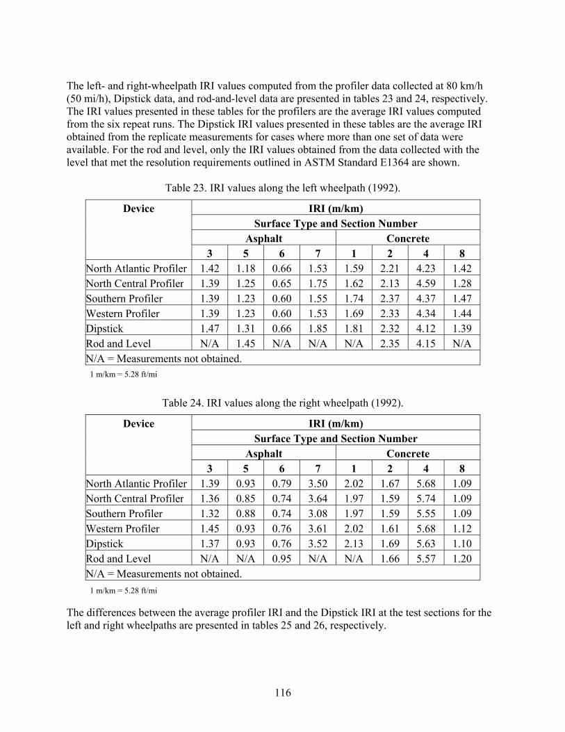
The lef(50 mi/ ely. The IR d from thobtaineavailablevel th

(m/km)

t- and right-wheelpath IRI values computed from the profiler data collected at 80 km/h h), Dipstick data, and rod-and-level data are presented in tables 23 and 24, respectivI values presented in these tables for the profilers are the average IRI values computee six repeat runs. The Dipstick IRI values presented in these tables are the average IRI d from the replicate measurements for cases where more than one set of data were le. For the rod and level, only the IRI values obtained from the data collected with the at met the resolution requirements outlined in ASTM Standard E1364 are shown.

Table 23. IRI values along the left wheelpath (1992).

Device IRI Surface Type and Section Number Asphalt Concrete

3 5 6 7 1 2 4 8 No Profilerth Atlantic r 1.42 1.18 0.66 1.53 1.59 2.21 4.23 1.42 North Central Profiler 1.39 1.25 0.65 1.75 1.62 2.13 4.59 1.28 Southern Profiler 1.39 1.23 0.60 1.55 1.74 2.37 4.37 1.47 Western Profiler 1.39 1.23 0.60 1.53 1.69 2.33 4.34 1.44 Dipstick 1.47 1.31 0.66 1.85 1.81 2.32 4.12 1.39 Rod and Level N/A 1.45 N/A N/A N/A 2.35 4.15 N/A N/A = Measurements not obtained.

Table 24. IRI values along the right wheelpath (1992).

Device IRI (m/km) Surface Type and Section Number Asphalt Concrete

3 5 6 7 1 2 4 8 North Atlantic Profiler 1.39 0.93 0.79 3.50 2.02 1.67 5.68 1.09 North Central Profiler 1.36 0.85 0.74 3.64 1.97 1.59 5.74 1.09 Southern Profiler 1.32 0.88 0.74 3.08 1.97 1.59 5.55 1.09 Western Profiler 1.45 0.93 0.76 3.61 2.02 1.61 5.68 1.12 Dipstick 1.37 0.93 0.76 3.52 2.13 1.69 5.63 1.10 Rod and Level N/A N/A 0.95 N/A N/A 1.66 5.57 1.20 N/A = Measurements not obtained.

1 m/km = 5.28 ft/mi The differences between the average profiler IRI and the Dipstick IRI at the test sectileft and right wheelpaths are presented in tables 25 and 26, respectively.

ons for the

1 m/km = 5.28 ft/mi

116

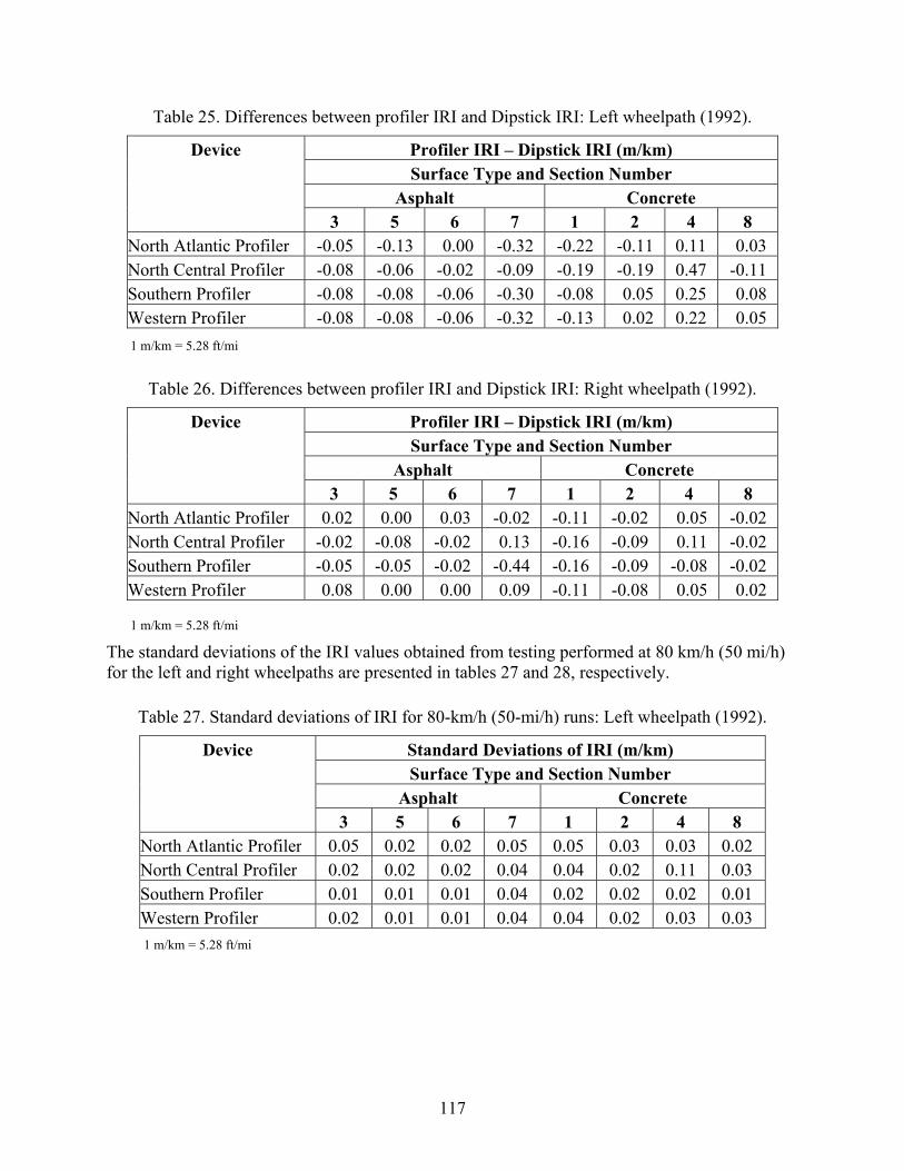
Table 25. Differences between profiler IRI and Dipstick IRI: Left wheelpath (1992).

Device Profiler IRI – Dipstick IRI (m/km) Surface Type and Section Number Asphalt Concrete

3 5 6 7 1 2 4 8 North Atlantic Profiler -0.05 -0.13 0.00 -0.32 -0.22 -0.11 0.11 0.03 North Central Profiler -0.08 -0.06 -0.02 -0.09 -0.19 -0.19 0.47 -0.11 Southern Profiler 0.25 0.08 -0.08 -0.08 -0.06 -0.30 -0.08 0.05Western Profiler -0.08 -0.08 -0.06 -0.32 -0.13 0.02 0.22 0.05

Table 26. ifferences between pro ipstick IRI: Right wheelpath (1992).

ro IR ps R m

D filer IRI and D

Device P filer I – Di tick I I (m/k ) ur y d n eS face T pe an Sectio Numb r h ncAsp alt Co rete

3 5 6 7 1 2 4 8 North Atlantic Profiler 0.02 0.00 0.03 -0.02 -0.11 -0.02 0.05 -0.02North Central Profiler -0.02 -0.08 -0.02 0.13 -0.16 -0.09 0.11 -0.02S 05 -0.02 -0.44 -0.16 -0.09 -0.08 -0.02 outhern Profiler -0.05 -0.W 0.08 0.00 0.00 0.09 -0.11 -0.08 0.05 0.02 estern Profiler

The standard deviatio 80 km/h (50 mi/h) for the left and right wheelpaths are presented in tables 27 and 28, respectively.

able 27. Standard deviations of IR

Device Standard Deviations of IRI (m/km)

ns of the IRI values obtained from testing performed at

m/h (50-mi/h) runs: Left wheelpath (1992). T I for 80-k

Sur y d n eface T pe an Sectio Numb r Asph cralt Con ete

3 5 6 7 1 2 4 8 North Atlantic Profiler 0.05 0.02 0.02 0.05 0.05 0.03 0.03 0.02 North Central Profiler 0.02 0.02 0.02 0.04 0.04 0.02 0.11 0.03 Southern Profiler 0.01 0.01 0.01 0.04 0.02 0.02 0.02 0.01 Western Profiler 0.02 0.01 0.01 0.04 0.04 0.02 0.03 0.03

1 /km = 5

1 m/km = 5.28 ft/mi

m .28 ft/mi

1 m/km = 5.28 ft/mi

117

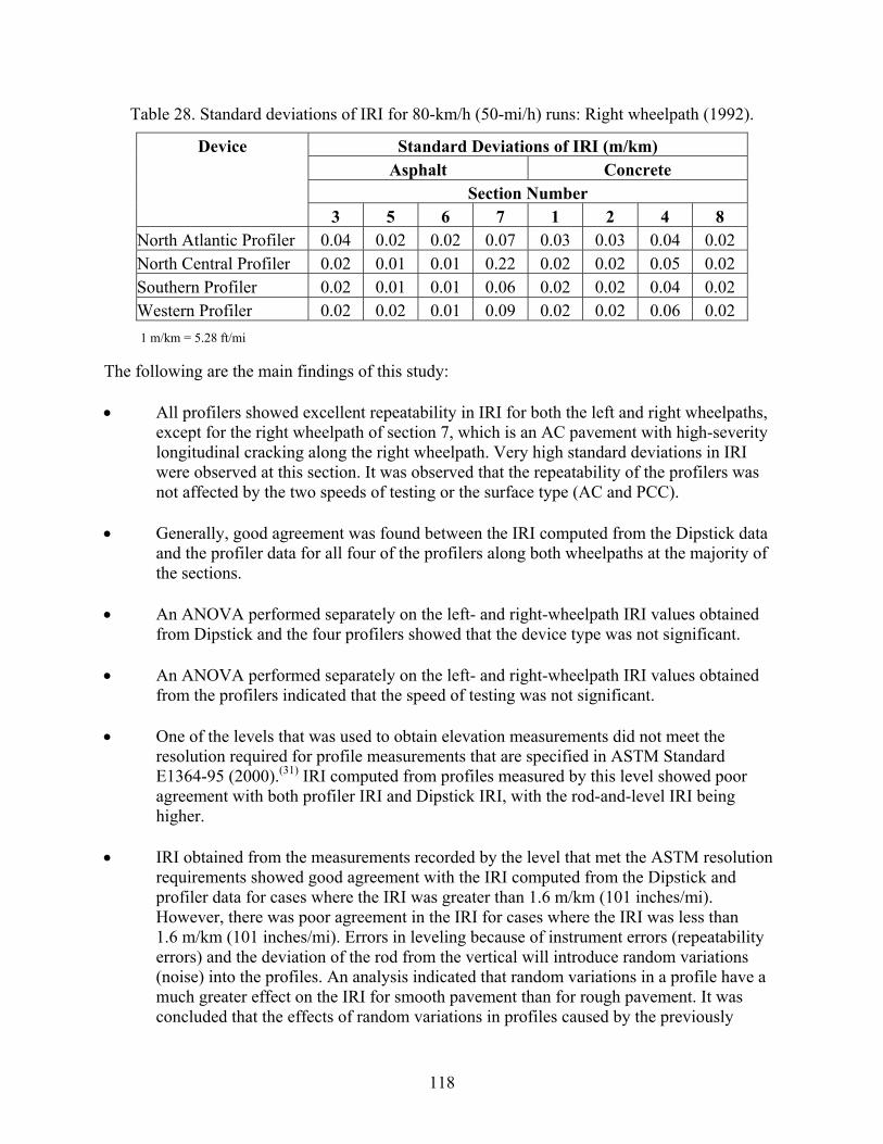
Ta ).

ble 28. Standard deviations of IRI for 80-km/h (50-mi/h) runs: Right wheelpath (1992

Device Standard Deviations of IRI (m/km) A e sphalt Concret

Section Number 1 2 4 83 5 6 7

North Atlantic Profiler 0 0 0.0.04 0.02 0.02 0.07 0.03 .03 .04 02 North Central Profiler 0 0 00.02 0.01 0.01 0.22 0.02 .02 .05 .02 Southern Profiler 0. 0 0.0.02 0.01 0.01 0.06 0.02 02 .04 02 Western Profiler 0. 0 0.0.02 0.02 0.01 0.09 0.02 02 .06 02

The f • All t repe ht wheelpaths,

except for the right wheelpath of se h high-severity longitudinal cracking along the right wheelpath. Very high standard deviations in IRI were observed at this section. It was observed that the repeatability of the profilers was

two ing or the e C CC • ree a d n I the Dipstick data

r data f ou e rs b e a a f

performed separately on the left- and right-wheelpath IRI values obtained

• An ANOVA performed separately on the left- and right-wheelpath IRI values obtained

• One o els that was used to meet the

resolution required for profile meas Standard E1364-95 (2000).(31) IRI compute ofiles measured by this level showed poor agreement with both profiler IRI and Dipstick IRI, with the rod-and-level IRI being

• e m em re b le at e tion

owed g re t w e IRI com f e ckr cases w th a te 1 i

e was poor agreement in the IRI for cases where the IRI was less than 1.6 m/km (101 inches/mi). Errors in leveling because of instrument errors (repeatability errors) and the deviation of the rod from the vertical will introduce random variations (noise) into the profiles. An analysis indicated that random variations in a profile have a much greater effect on the IRI for smooth pavement than for rough pavement. It was concluded that the effects of random variations in profiles caused by the previously

i 1 m/km = 5.28 ft/m

ollowing are the main findings of this study:

profilers showed excellen atability in IRI for both the left and rigction 7, which is an AC pavement wit

not affected by the speeds of test s acurf ty (Ape Pand ).

Generally, good ag ment w s foun betwee the IR computed fromand the profile or all f r of th profile along oth wh elpaths t the m jority othe sections.

An ANOVA•from Dipstick and the four profilers showed that the device type was not significant.

from the profilers indicated that the speed of testing was not significant.

f the lev obtain elevation measurements did not urements that are specified in ASTM

d from pr

higher.

IRI obtained from th easur ents corded y the vel th met th ASTM resolurequirements sh ood ag emen ith th puted rom th Dipsti and profiler data fo here e IRI w s grea r than .6 m/km (101 inches/m ). However, ther

118

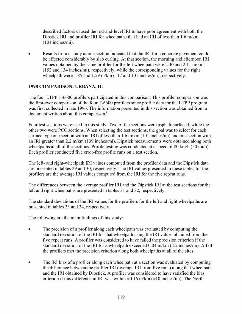
described factors caused the rod-and-level IRI to have poor agreement with both the Dipstick IRI and profiler IRI for wheelpaths that had an /km (101 i).

• Results f m a study at one section indicated oncrete pavement could

be affected considerably by slab curling. At that section, the morning and afternoon IRI e r fo ef lp er a 1

/mi e , th es g s r an m (1 1 ch , ti

1998 : URBA L

he four LTPP T-6600 profilers participated in this comparison. This profiler comparison was rs since profile data for the LTPP program

as first collected in late 1996. The information presented in this section was obtained from a cume

Four te e other twsurface ection with n IRI greater than 2.2 m/km (139 inches/mi). Dipstick measurements were obtained along both

Each pr

he left- and right-wheelpath IRI values computed from the profiler data and the Dipstick data

profiler

left and

are

present

The fol The precision of a profiler along each wheelpath was evaluated by computing the

. All of

• g

IRI of less than 1.6 minches/m

ro that the IRI for a c

values obtained by th same p ofiler r the l t whee ath w e 2.40 nd 2.1 m/km(152 and 134 inches

1.85), resp ctively while e corr pondin value for the ight

wheelpath were d 1.59 /km 17 and 01 in es/mi) respec vely.

COMPARISON NA, I Tthe first-ever comparison of the four T-6600 profilewdo nt written about this comparison.(13)

st sections were used in this study. Two of the sections were asphalt-surfaced, while tho were PCC sections. When selecting the test sections, the goal was to select for each

type one section with an IRI of less than 1.6 m/km (101 inches/mi) and one sawheelpaths at all of the sections. Profile testing was conducted at a speed of 80 km/h (50 mi/h).

ofiler conducted five error-free profile runs on a test section.

Tare presented in tables 29 and 30, respectively. The IRI values presented in these tables for the

s are the average IRI values computed from the IRI for the five repeat runs.

The differences between the average profiler IRI and the Dipstick IRI at the test sections for the right wheelpaths are presented in tables 31 and 32, respectively.

The standard deviations of the IRI values for the profilers for the left and right wheelpaths ed in tables 33 and 34, respectively.

lowing are the main findings of this study:

•standard deviation of the IRI for that wheelpath using the IRI values obtained from the five repeat runs. A profiler was considered to have failed the precision criterion if thestandard deviation of the IRI for a wheelpath exceeded 0.04 m/km (2.5 inches/mi)the profilers met the precision criterion along both wheelpaths at all of the sites.

The IRI bias of a profiler along each wheelpath at a section was evaluated by computinthe difference between the profiler IRI (average IRI from five runs) along that wheelpath and the IRI obtained by Dipstick. A profiler was considered to have satisfied the bias criterion if this difference in IRI was within ±0.16 m/km (±10 inches/mi). The North

119

Atlantic, Southern, and Western profilers passed the bias criterion for both wheelpathall of the test sections. The North Central profiler passed the bias criterion for all ofcases, except for t

s at the

he right wheelpath of the rough AC section (section 2). The variability in the IRI values obtained by the North Central profiler for the repeat runs is considered

to be the cause of the profiler failing the bias criterion at this section.

Table 29. IRI values along the left wheelpath (1998).

Device IRI (m/km) Surface Type and Section Number Asphalt Concrete

1 2 3 4 North Atlantic Profiler 1.02 2.49 1.30 2.77 North Central Profiler 1.04 2.55 1.28 2.90 Southern Profiler 1.02 2.56 1.27 2.83 Western Profiler 1.02 2.59 1.28 2.90 Dipstick 0.95 2.52 1.17 2.87

Table 30. IRI values along the right wheelpath (1998).

Device IRI (m/km)

1 m/km = 5.28 ft/mi

Surface Type and Section Number Asphalt Concrete

1 2 3 4 North Atlantic Profiler 1.08 2.38 1.26 3.09 North Central Profiler 1.05 2.62 1.24 3.17 Southern Profiler 1.04 2.39 1.24 3.05 Western Profiler 1.04 2.50 1.22 3.20 Dipstick 0.96 2.46 1.13 3.17

1 m/km = 5.28 ft/mi

Table 31. Differences between the profiler IRI and Dipstick IRI: Left wheelpath (1998).

Device Profiler IRI – Dipstick IRI (m/km) Surface Type and Section Number Asphalt Concrete

1 2 3 4 North Atlantic Profiler 0.07 -0.03 0.13 -0.10 North Central Profiler 0.09 0.03 0.11 0.03 Southern Profiler 0.07 0.04 0.10 -0.04 Western Profiler 0.07 0.07 0.11 0.03

1 m/km = 5.28 ft/mi

120

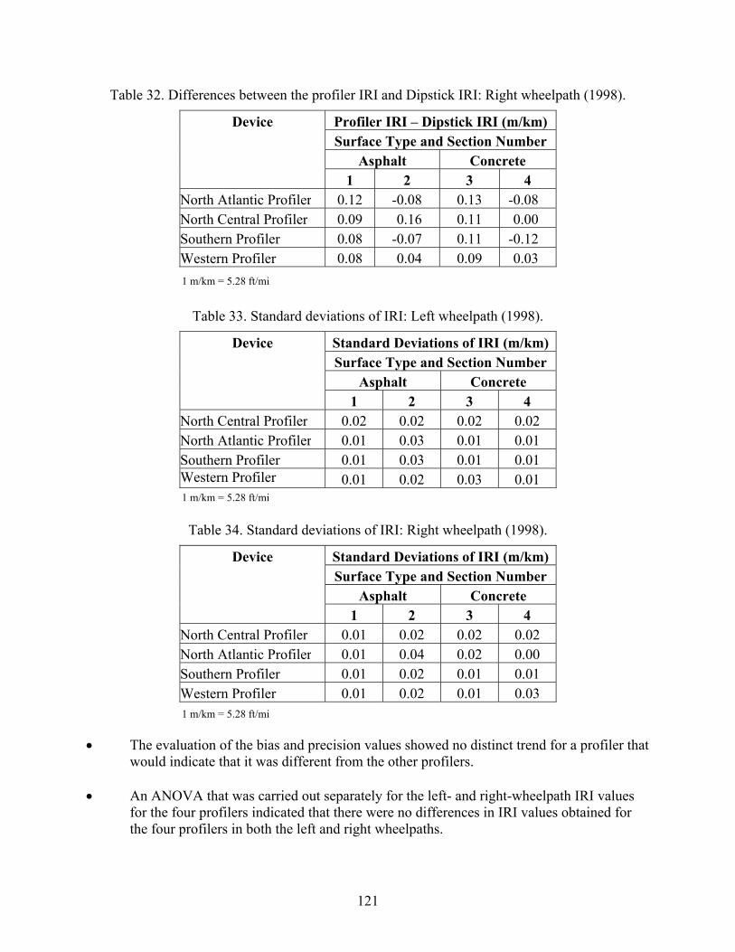
Table 32. Differences between the profiler IRI and Dipstick IRI: Right wheelpath (1998).

Device Profiler IRI – Dipstick IRI (m/km) Surface Type and Section Number Asphalt Concrete

1 2 3 4 North Atlantic Profiler 0.12 -0.08 0.13 -0.08 North Central Profiler 0.09 0 0.00 .16 0.11Southern Profiler 0.08 -0.07 0.11 -0.12 Western Profiler 0.0 4 0. 8 0.0 09 0.03

evia f IRI: Left wheelpath (1998).

Standard Deviations of IRI (m/km)

Table 33. Standard d tions o

Device Surface Type and Section Number Aspha ncrelt Co te

1 2 3 4 North Central Profiler 0.02 0.02 0.02 0.02 North Atlantic Profiler 0.01 0.03 0.01 0.01 Southern 0.01 0.03 0.01 0.01 ProfilerWestern Profiler 0.01 0.02 0.03 0.01

Table 34. Standard deviations of IRI: Right wheelpath (1998).

Standard Deviations of IRI (m/km) Device Surface Type and Section Number Aspha ncrelt Co te

1 2 3 4 North Central Profiler 0.01 0.02 0.02 0.02 North Atlantic Profiler 0.01 0.04 0.02 0.00 Southern Profiler 0.01 0.02 0.01 0.01 Western Profiler 0.01 0.02 0.01 0.03

• The evaluation of the bias and precision values wed n

would indicate that it was diffe nt fr e oth fil • An ANO t sep for ft- ght- path IRI values

for the f ted that th ere no differences in IRI values obtained for the four e left and hee .

1 m/km = 5.28 ft/mi

m/km = 5.28 ft/mi

m/km = 5.28 ft/mi

1

1

shor p

o drs.

istinct trend for a profiler that re o hm t e ro e

VA that was carried ou arately the le and ri wheelour profilers indica ere wprofilers in both th right w lpaths

121

• for the North Atla rth Centr ing wavebands: (1) 1 to 3 m (3 t (2) less 66 ft), and (4) 20 to 0 m (66 to 100 ft). The S results, except for the r gh PCC site. At this site, the profiler s repeatability for wavebands between 10 and 20 m (33 and 66 ft), and 20 and 30 m (66 and 100 ft), with the repe th r w d. T y be caused by the conditio een rofi and hic er completion of the com ion een ofile nd filer vehicle in the Southern profiler were inspected and tightened. Subsequent te ndicated that this profiler was able to collect repeatab file n rou ctio

2000 COMPARISON: COLLEGE STATION The four LTPP T-6600 profilers participated in ththis section was obtained ocumen Five pavement sections were used for profile testing: (1) a smooth AC site, (2) a medium-rough AC site, (3) a chip-seal secti , (4) a smooth PCC site, and (5) a rough PCC site. The smooth AC and the medium within the Riverside Cam xas A&M University and ectio certi Tex part of Transportation (TxDOT) profil ute measuremenprofiler were av o section ev wal rofi ta for these two sections were no y TxDOT use sites sed tifying profilers. Measurements m ence device (e.g., Dipstick or a walking profiler) were not performed at the other three test sections. Profile testing was conducted at a speed of 80 km/h (50 mi/h). Each profi ction. The IRI values computed e profiler the left and right wheelpaths on the tests sections are p ely. The IRI values presented in these tables for the profiler verage IR mputed from the IRI for the five repeat runs. The differences file nd alking Profiler t the test sections are presented in The standard de I values f prof or th and wheelpaths are presented in tables 38 and 39, respectively.

A visual review of the profile data plots indicated excellent repeatability of the profilesntic, No

o 100 ft),al, and Western profilers for the followthan 10 m (33 ft), (3) 10 to 20 m (33 to0

3 outhern profiler also exhibited similarou Southern howed poor

atability being poorer for e latte aveban his man of the connection betw

nnect the p ler bar the ve le. Aft

parison test, the co s betw the pr r bar a the prosting i

le pro data o gh se ns.

, TX

is comparison. The information presented in from a d t written about this comparison.(13)

on-rough AC sections were located

are used as calibration spus of Te

ns to fy the as De ment ers. The IRI values comp d from ts made with an ARRB walking ailable for these tw s. How er, the king p ler dat made available b beca these are u for cerade with a refer

ler was required to obtain five error-free profile runs on a test se

from th data and the walking profiler data for resented in tables 35 and 36, respectiv

s are the a I values co

between the average pro table 37.

r IRI a the W IRI a

viations for the IR or the ilers f e left right

122

Table 35. IRI values along the left wheelpath (2000).

Device IRI (m/km) Test Section Smooth Medium Chip Smooth Rough AC AC Seal PCC PCC

North Atlantic Profiler 1.13 1.93 3.00 1.54 2.94 North Central Profiler 0.98 1.81 2.72 1.52 2.68 Southern Profiler 1.01 1.85 3.31 1.48 2.78 Western Profiler 1.04 1.94 3.33 1.56 2.90 Walking Profiler 1.01 1.85 N/A N/A N/A N/A = Measurements not performed.

1 m/km = 5.28 ft/mi

Table 36. IRI values along the right wheelpath (2000).

Device IRI (m/km) Test Section Smooth Medium Chip Smooth Rough AC AC Seal PCC PCC

North Atlantic Profiler 0.72 1.77 2.02 1.70 2.95 North Central Profiler 0.79 1.75 2.77 1.68 2.92 Southern Profiler 0.73 1.81 1.98 1.63 2.96 Western Profiler 0.66 1.72 2.11 1.63 2.88 Walking Profiler 0.67 1.75 N/A N/A N/A N/A = Measurements not performed.

Table 37. Differences between the profiler IRI and the walking profiler IRI (2000).

(m/km)

1 m/km = 5.28 ft/mi

Section Wheelpath Average Profiler IRI – Reference IRI

Profiler North North Southern Western Atlantic Central

Smooth Asphalt Left 0.12 -0.03 0 0.03 Smooth Asphalt Left 0.08 -0.04 0 0.09 Medium Asphalt Right 0.05 0.12 0.06 -0.01 Medium Asphalt Right 0.02 0 0.06 -0.03

1 m/km = 5.28 ft/mi

123

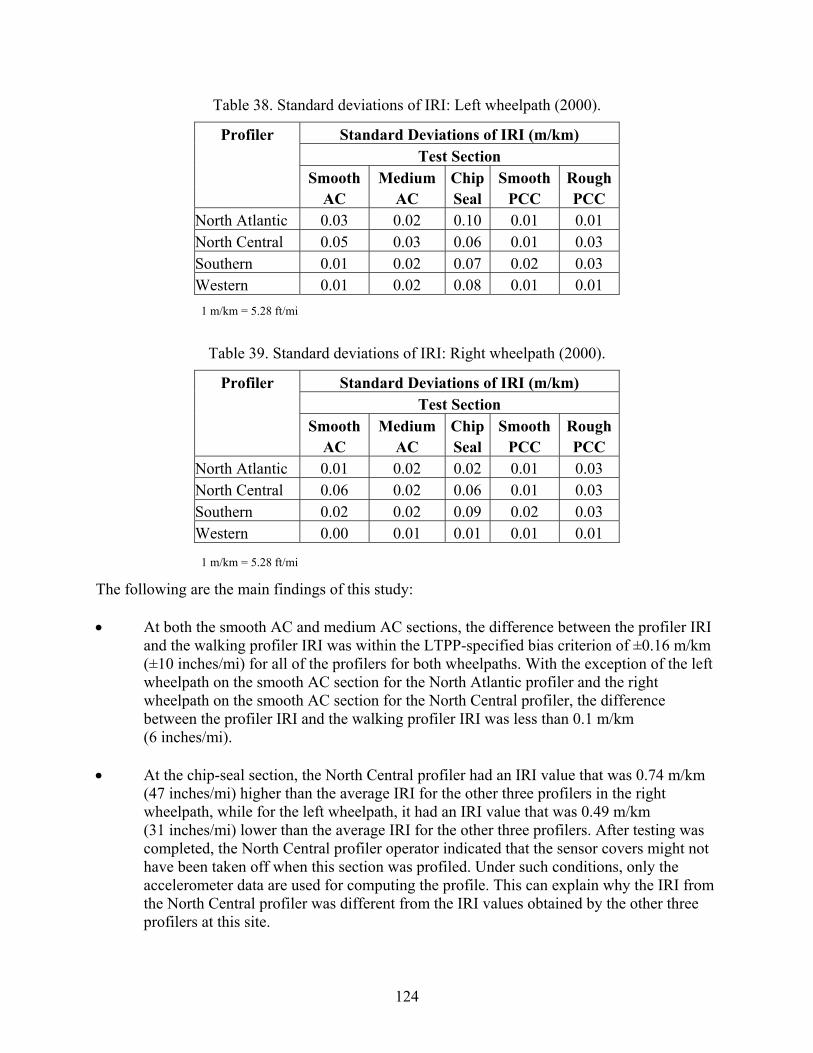
Table 38. Standard deviations of IRI: Left wheelpath (2000).

Profiler Standard Deviations of IRI (m/km) Test Section Smooth Medium th Rough Chip Smoo A A a CC C Se l PCC P C North Atlantic 0.03 0.02 0.1 .0 0.0 0 0 1 1 North Central 0.0 0.0 0.0 .01 0.05 3 6 0 3 Southern 0.0 0.0 0.0 .02 0.03 1 2 7 0 Western 0.0 0.0 0.0 .01 0.01 1 2 8 0

IRI: Right wheelpath (2000).

Profiler Standard Deviations of IRI (m/km)

Table 39. Standard deviations of

Test Section Smooth Medium Rough Chip Smooth AC AC C PCC Seal PCNorth Atlantic 0.01 0.02 0.02 0.01 0.03 North Central 0 0 0 ..06 .02 0. 6 0.01 0 03 Southern 0.02 0.02 0.0 .0 0.03 9 0 2 Western 0.0 0.0 0.0 .01 0.01 0 1 1 0

The following are the main findings of this study: • At b ctions, the difference between e profiler IRI

and the walking profiler IRI was within the LTPP-specified bias criterion of ±0.16 m/km (±10 l of the profilers fo both wheelpaths. With the exception of the left

between er IR lk(6 inches/mi).

• At the chip-seal section, the orth Ce ofi n h 4 m/km

(47 inches/m higher than th avera t hwh r th heelp a ue th as 0.49 (3 r th average r the other three profilers. A sting was co C iler operator in that sensor might not ha h section rofile er su diti ly the ac e r compu he profile. This can explain why the IRI from the ofiler was different f m the IRI values obtained by the other three profilers at this site.

mi

i

1 m/km = 5.28 ft/

1 m/km = 5.28 ft/m

oth the smooth AC and medium AC se th

inches/mi) for al r wheelpath on the smooth AC section for the North Atlantic profiler and the right wheelpath on the smooth AC section for the North Central profiler, the difference

the profil I and the wa ing profiler IRI was less than 0.1 m/km

N ntral pr ler had a IRI value tree p

at was 0.7i)h

e w

ge IRI forath, it had

he other tn IRI val

rofilers in the right t weelpath, w ile fo

1 inches/mi) lowee leftan the

a /kmfter tem

IRI fompleted, the North entral prof dicated the coversve been taken off w en this was p d. Und ch con ons, oncelerometer data ar used fo ting t North Central pr ro

124

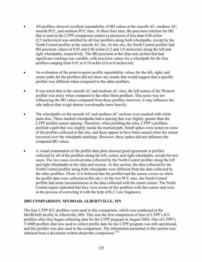
• All profile C, medium AC, smooth PCC ium PC criterion for IRI that is used in the LTPP comp .04 m/km (2.5 inches/mi)) was satisfied by all four profilers along both wheelpaths, except by the North C tral profiler at t it t l profiler had IRI prec ion values of 0.05 0.06 m i) along the left and right wh tiv e IRI sion chip-seal section that had signific s va , with ion s f heel or the four profilers ranging from 0.01 0 m/k 6 to es

• An evaluation of the point-to-point profile repeatability values for the left, right, and

center paths for the profilers did not show any trends that would suggest that a specific profiler was different when compared to the other profilers.

• It was noted that at the smooth AC a Western

profiler was noisy when comp ise was not influencing the IRI values computed from however, it may influence the ride ind s that weigh sh e r i

• The wheelpaths on the smooth AC and um cti ere m with white

paint do d w aths h pac t w ghtl ter than the LTPP p acing. Therefore, when p g es, L s profilers profiled t was slig nside arke . S pike e noted on some of the p lected at t e, and ap h en c when the sensor traversed over the wheelpath markings. However, these spikes did not influence the compute

A visual examination of the profile data plots showed good agreement in profiles

d by hen

ntral e inconsistencies in the data collected with the center sensor. The North

Central region indicated that they were aware of this problem with this sensor and were

2003 C The fouMn/RO profilerT-6600 , and this profiler was also used in the comparison. The information presented in this section was btained from a document written about this comparison.(15)

rs showed excellent repeatability of IRI values at the smooth A, and med C sites. At these four sites, the precision

arison studies (a precision of less than 0

en the smooth AC site. A this s e, the Nor h Centrais and /km (3.2 and 3.8 inches/meelpaths, respec ely. Th preci at the

ant cracking wa

riable precis value or a w path f to 0.1 m (0. 6 inch /mi).

nd medium AC sites, the left sensor of the ared to the other three profilers. This no

these profiles; ly. ice orter wav lengths mo e heav

mediad a s

AC seing tha

ons was sli

arkedy greats. These marke heelp

rofiler sensor sp rofilin the sit TPP’ a path tha htly i the m d path mall s s werrofiles col his sit these pear to ave be aused

d IRI values. •

collected by all of the profilers along the left, center, and right wheelpaths, except for two cases: The two cases involved data collected by the North Central profiler along the left and right wheelpaths at the chip-seal section. At this section, the data collected by the North Central profiler along both wheelpaths were different from the data collectethe other profilers. (Note: It is believed that the profiler had the sensor covers on wthe profile data were collected at this site.) At the two PCC sites, the North Ceprofiler had som

in the process of correcting it with the help of K.J. Law Engineers.

OMPARISON: MN/ROAD, ALBERTVILLE, MN

r LTPP ICC profilers were used in this comparison, which was conducted at the AD facility in Albertville, MN. This was the first comparison of four of LTPP’s ICCs after they began collecting data for the LTPP program in August 2002. One of LTPP’s profilers that was used to collect profile data for the LTPP program was still operational

o

125

st sections were used for profile testing: (1) a smooth AC section, (2) a rough AC section

ooth PCC section, (4) a medium-rough PCC section, and (5) a chip-seal section.ements were obtained along both wheelpaths at all of the test sections. Profile testing wated at a speed of 80 km/h (50 mi/h). Each profiler was required to obtain five error-free runs on a test section.

t- and right-wheelpath IRI values computed from the profiler data and the Dipstick daented in tables 40 and 41, respectively. The IRI values presente

Five te , (3) a sm Dipstick measur s conducprofile The lef ta are pres d in these tables for the

rofilers are the average IRI values computed from the IRI for the five repeat runs. p

Table 40. IRI values along the left wheelpath (2003).

Device IRI (m/km) Section 1 Section 2 Section 3 Section 4 Section 5 SealSmooth AC Rough AC Smooth PCC Medium PCC Chip North Atlantic: ICC 1.27 2.76 0.92 1.45 2.25 Nort 1.57 2.15 h Central: ICC 1.26 2.75 0.93 Southern: ICC 1.29 2.78 0.93 1.45 2.15 Western: ICC 1.28 2.75 0.91 1.43 2.20 K.J. Law Engineers 1.31 2.75 0.94 1.47 2.25 Dipstick 1.17 2.80 0.88 1.32 2.24

Table 41. IRI values along the right wheelpath (2003).

Device IRI (m/km) Section 1 Section 2 Section 3 Section 4 Section 5 Smooth AC Rough AC Smooth PCC Medium PCC Chip SealNorth Atlantic: ICC 1.68 2.81 0.98 1.70 2.54 North Central: ICC 1.73 3.01 1.02 1.72 2.54 Southern: ICC 1.69 2.62 0.96 1.67 2.54 Western: ICC 1.66 2.54 0.97 1.71 2.50 K.J. Law Engineers 1.64 2.46 0.96 1.70 2.44 Dipstick 1.81 2.79 0.99 1.64 2.63

1 m/k

1 m/km = 5.28 ft/mi

m = 5.28 ft/mi

The differences between the average profiler IRI and the Dipstick IRI on the test sections for the left and right wheelpaths are presented in tables 42 and 43, respectively.

126

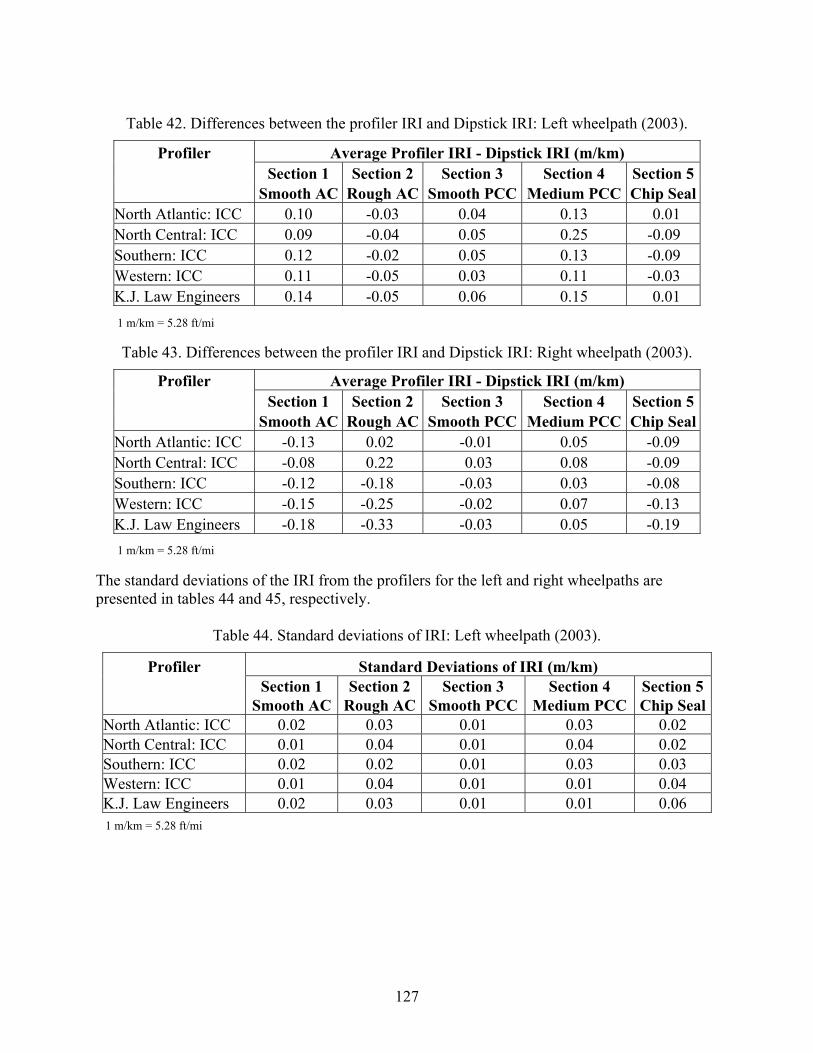
Table 42. Differences between the profiler IRI and Dipstick IRI: Left wheelpath (2003).

Profiler Average Profiler IRI - Dipstick IRI (m/km) Section 1 Section 2 Section 3 Section 4 Section 5 Smooth AC Rough AC Smooth PCC Medium PCC Chip SealNorth Atlantic: ICC 0.10 -0.03 0.04 0.13 0.01 North Central: ICC 0.09 -0.04 0.05 0.25 -0.09 Southern: ICC 0.12 -0.02 0.05 0.13 -0.09 Western: ICC 0.11 -0.05 0.03 0.11 -0.03 K.J. Law Engineer 0.01 s 0.14 -0.05 0.06 0.15

an I: R pa

Profiler i i

Table 43. Differences between the profiler IRI d Dipstick IR ight wheel th (2003).

Average Prof ler IRI - Dipst ck IRI (m/km) Section 1 Section 2 Section 3 Section 4 Section 5 Smooth AC Rough AC Smooth PCC Medium PCC Chip SealNorth Atlantic: ICC -0.13 0.02 -0.01 0.05 -0.09 North Central: ICC -0.08 0.22 0.03 0.08 -0.09 Southern: ICC -0.12 -0.18 -0.03 0.03 -0.08 Western: ICC -0.15 -0.25 -0.02 0.07 -0.13 K.J. Law Engineers -0.18 -0.33 -0.03 0.05 -0.19

The standard deviations of the IRI from the profilers for the left and right wheelpaths are presented in tables 44 and 45, respectively.

Table 44. Standard deviations of l

Standard Deviations of IRI (m/km)

1 m/km = 5.28 ft/mi

1 m/km = 5.28 ft/mi

IRI: Left whee path (2003).

Profiler Section 1 Section 2 Section 3 Section 4 Section 5 Smooth AC Rough AC Smooth PCC Medium PCC Chip Seal

North Atlantic: ICC 0.02 0.03 0.01 0.03 0.02 North Central: ICC 0.01 0.04 0.01 0.04 0.02 Southern: ICC 0.02 0.02 0.01 0.03 0.03W 0.01 0.04 0.01 0.01 0.04 estern: ICC K.J. Law Engineers 0.02 0.03 0.01 0.01 0.06

1 m/km = 5.28 ft/mi

127

P

Table 45. Standard deviations of IRI: Right wheelpath (2003).

rofiler Standard Deviations of IRI (m/km) Section 1 Section 2 Section 3 Section 4 Section 5 S lmooth AC Rough AC Smooth PCC Medium PCC Chip Sea

North Atlantic: ICC 0 .07 0.11 0.02 0.02 0.02North Central: ICC 0 .01 0.13 0.01 0.01 0.03S 0 outhern: ICC .07 0.08 0.02 0.03 0.04W 0 estern: ICC .08 0.09 0.01 0.01 0.03K 0 .J. Law Engineers .04 0.08 0.02 0.02 0.03

The • Overall, all of the profilers ap se data did

not indicate that a particular profiler was behaving differently than the other profilers as far as IRI repeata e

n stu that th standard deviations from iple rune less .5 inches owever, times this criterion distr re pre ong the wheelpath, because even a slight shift in

iled can signif pact on IRI. The IRI precision criterion was of the case pt for llowing: profilers, except for the North

along ht wh h of the s AC secti along the right wheelpath of the rough AC section (section 2); (3) left

wheelpath of the rough AC section (section 2) and medium-rough PCC section ction

s profiler. Distresses were present along the right wheelpath on the smooth AC section (section 1) and along both wheelpaths on the rough AC section rs was the most

se of the failure of the p t these two sites. • Good agreement i o

LT u o iepstick nd the p r IRI should be within ±0 km

ion wa for all of xcep e follow ) elpath of th oth AC n (sectio d the chip-seal section (section 5)

.J. Law Eng profiler eft wheelpath of the medi ugh PCC on the No ntral pr , and (3) heelpath o rough AC ion

by all profilers, except for the North Atlantic profiler. Extensive distresses were present on the rough AC section (section 2), and the failure of the profilers to meet the specified criterion at this site may be caused by the differences in the way downward features in the pavement are measured by Dipstick and the profilers.

• An evaluation of the profile data collected by the North Central, North Atlantic, and

Western ICC profilers indicated that the profile data collected by these profilers generally

1 m/km = 5.28 ft/mi

main findings of this study are:

pear to be obtaining repeatable IRI values. The

bility is concerned. The pr cision criterion for IRI that is used in the LTPP compariso dies is e IRI mult s on a section should b

et if than 0.04 m/km (2 /mi). H some

cannot be mthe path prof

esses ahave a

sent alicant im

met for all s, exce the fo (1) all Central profiler the rig eelpat mooth on (section 1); (2) all of the profilers

(section 4) for the North Central profiler; and (4) left wheelpath of the chip-seal se(section 5) for the K.J. Law Engineer

(section 2), and variability on the paths profiled by the profilelikely cau rofilers to meet the specified criterion a

between profPP criterion

ler IRI and Dsed for the c

ipstick IRI wasmparison stud

btained for the ms is that the diffe

ajority of rence the cases. The

between the Di IRI a rofile .16 m/(±10 inches/mi). This criter s met the cases, e t for th ing: (1right whe e smo sectio n 1) anby the K ineers , (2) l um-ro secti(section 4) by rth Ce ofiler right w f the sect(section 2)

128

have similar repeatability. The K.J. Law ngineers and Southern ICC profilers showed much hig lpaths when

to the other three ICC p btained by the rofilers te file

capturing similar r f e p t l leother ation wa ormed to tigate the r bility oflected e Southern profiler. This investigation indicated that t

profiler wa ining re le profil that was co able to th by the othe ICC profilers on the Mn/ROAD test sections. The poor profile

taine e Southern profiler on the Mn/ROAD test sections m e d by problems with the operational procedures that were followed by the

profiler operator (e.g., insufficient lead-in, not maintaining a constant speed, etc.).

Collection of profile data at speeds of 35, 50, 65, 80, 95, and 110 km/h (22, 38, 41, 50,

•

utes the

between RoadRuf and ProQual.

Eher variability in the profile data for repeat runs along both whee

comparedfour ICC p

rofilers. A comparison of the profiles oindi ll fou on the five st sections cated that a r of the pro rs are

profile featuhe profiles co

es. A profilelected by the

eature that appother ICC profi

ared in any ICC rs. After the pro

rofiler wasfiler also esent on

comparison, an pr

evalu s perf inves epeata the profile data col by th he Southern s obta peatab e data mpar e dataobtained r threerepeatability ob d by th ay havbeen cause

•

59, and 69 mi/h) was performed by the K.J. Law Engineers and Southern ICC profilers on one section. The analysis of the data indicated that the IRI value did not appear to be influenced by the speed of testing.

There were differences in IRI values computed for the Dipstick data using ProQual and RoadRuf. RoadRuf is a software program developed by UMTRI. However, a comparison of IRI values obtained by ProQual and RoadRuf for profiler data showed that the IRI values were similar. For the Dipstick data collected along 10 wheelpaths (from 5 sections), the differences in the IRI values from ProQual and RoadRuf ranged from 0.004 to 0.079 m/km (0.25 to 5 inches/mi), with the IRI values from ProQual beinghigher than those obtained by RoadRuf for all of the cases. When ProQual compIRI from the Dipstick data, it first applies a filter that has an upper-wavelength cutoff of 100 m (328 ft), then it uses the filtered data to compute the IRI value. When RoadRuf computes the IRI from the Dipstick data, the software uses the Dipstick elevation profile to compute the IRI without any prefiltering of the data. The filtering of the Dipstick data performed by ProQual may be the cause of the differences in the Dipstick IRI values

129

APPENDIX B: PROFILER VERIFICATION STUDIES 1996 VERIFICATION TEST In 1996, FHWA purchased four K.J. Law Engineers T-6600 profilers to replace the K.J. Law Engineers DNC 690 profilers that were used in the LTPP program. Each region compared the DNC 690 and T-6600 profilers before using the T-6600 profiler to collect profile data for the LTPP program. Each region used four test sections for the verification test; each test section was 152.4 m (500 ft) long. Two sections were surfaced with AC, while the other two were jointed PCC pavements. When selecting the test sections, the aim was to select two sections for each pavement type so that one section will have an IRI value of less than 1.6 m/km (101 inches/mi), and the other section will have an IRI value of greater than 2.2 m/km (139 inches/mi). Dipstick measurements were performed on both wheelpaths at all four test sections. Each profiler performed three measurement sequences at each test section, with one measurement sequence being performed on 1 day. A measurement sequence consisted of obtaining a set of profile runs (a minimum of five good profile runs) on a test section at test speeds of 64 and 80 km/h (40 and 50 mi/h). Therefore, at each section, each profiler collected six data sets (two speeds x three sequences). During testing, each profiler collected 24 data sets (4 test sections x 2 test speeds x 3 measurement sequences). The wheelpaths at the test sections were not marked, and the profiler drivers judged the location of the wheelpath when profiling the sections. The guidelines for testing recommended that concurrent measurements be made at the test sections with the two profilers with a minimum time lag between measurements. The guidelines also recommended that an effort should be made to obtain the three profiler measurement sequences for a test section on 3 consecutive days. Each RSC was asked to compute the IRI value of the profiler data and Dipstick data using ProQual. The bias in the IRI value of a profiler for a wheelpath on a test section was determined by computing the difference between the average profiler IRI at a specific speed for a data set (computed by averaging the IRI values obtained from replicate runs) and the Dipstick IRI. The profiler was deemed to have satisfied the IRI bias criterion if this difference in IRI was within ±0.16 m/km (±10 inches/mi). For each data set, the standard deviation of the IRI for each wheelpath was computed by using the IRI values obtained for the replicate profile runs. The precision of the profiler was evaluated by using this standard deviation of the IRI. The profiler was deemed to have satisfied the precision criterion if the standard deviation of the IRI was less than 0.04 m/km (2.5 inches/mi). Each RSC prepared a report documenting the results of this comparison test. (See references 24, 25, 26, and 27.) A summary of the findings contained in these reports is presented separately for the four regions. North Atlantic Region For all profiler testing, the same driver operated each profiler. A review of the report indicated that, in many cases, more than five repeat runs were conducted for each data set. Thereafter, five

131

runs were selected for computing the average IRI and the standard deviation of the IRI. It appears that t re reviewed to s es

btained for the 80-km/h (50-mi/h) profiler runs and IRI obtained from the Dipstick at were extracted from the report are presented in table 46. The

ifferences between the average profiler IRI and the Dipstick IRI for the profile runs obtained at

Table 46. Profiler IRI for 80-km/h (50-mi/h) runs and Dipstick IRI: North Atlantic region.

he five runs were selected after the IRI values from all available runs weelect values that were similar to each other. The average profiler IRI valu

omeasurements at the four sites thd80 km/h (50 mi/h) are presented in table 47. It should be noted that testing resulted in six data sets at each section, and these tables only show the results obtained for 80-km/h (50-mi/h) testing, which comprise three data sets from a test section.

Site Sequence Test Average IRI (m/km) Date Left Wheelpath Right Wheelpath T-6600 DNC 690 Dipstick T-6600 DNC 690 Dipstick

Smooth AC 1 10/07/96 0.78 0.86 0.83 0.89 0.87 0.92 2 10/09/96 0.74 0.86 0.88 0.86 3 10/10/96 0.75 0.87 0.87 0.86 Rough AC 1 10/07/96 2.44 2.26 2.30 1.92 1.89 1.91 2 10/09/96 2.11 2.27 1.67 1.92 3 10/10/96 2.28 2.28 1.72 1.87 Smooth PCC 1 10/03/96 1.19 1.25 1.27 1.37 1.30 1.39 2 10/04/96 1.18 1.22 1.34 1.31 3 10/04/96 1.20 1.21 1.40 1.33 Rough PCC 1 10/07/96 1.92 1.81 1.93 2.11 2.12 2.22 2 10/09/96 1.88 1.89 2.23 2.15 3 10/10/96 1.88 1.88 2.18 2.18 Note: Only one data set was obtained for Dipstick at each site.

Table 47. Differences between the profiler IRI and the Dipstick IRI: North Atlantic regio

Site Sequence Test Profiler IRI – Dipstick IRI (m/km)

1 m/km = 5.28 ft/mi

n.

Date Left Wheelpath Right Wheelpath T-6600 DNC 690 T-6600 DNC 690

Smooth AC 1 10/07/96 -0.05 0.03 -0.03 -0.05 2 10/09/96 -0.09 0.03 -0.05 -0.06 3 10/10/96 -0.08 0.04 -0.05 -0.06 Rough AC 1 10/07/96 0.14 -0.04 0.01 -0.02 2 10/09/96 -0.20 -0.04 -0.24 0.00 3 10/10/96 -0.02 -0.02 -0.20 -0.05 Smooth PCC 1 10/03/96 -0.08 -0.02 -0.03 -0.09 2 10/04/96 -0.09 -0.05 -0.05 -0.08 3 10/04/96 -0.07 -0.06 0.01 -0.06 Rough PCC 1 10/07/96 -0.01 -0.13 -0.11 -0.10 2 10/09/96 -0.05 -0.05 0.01 -0.08 3 10/10/96 -0.05 -0.05 -0.04 -0.04 1 m/km = 5.28 ft/mi

132

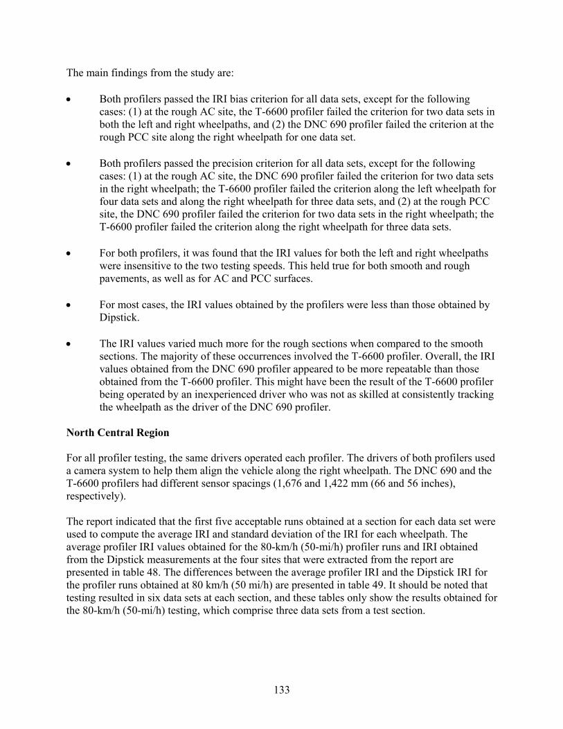
The main findings from the study are: • Both profilers passed the IRI bias criterion for all data sets, except for the followin

cases: (1) at the rough AC site, the T-6600 profiler failed the criterion for twoboth the left and right wheelpaths, and (2) the DNC 690 profiler failed the criterion at the rough PCC site along the right wheelpath for one data set.

• Both profilers passed the precision criterion for all data sets, except for the followin

cases: (1) at the rough AC site, the DNC 690 profile

g data sets in

g r failed the criterion for two data sets

in the right wheelpath; the T-6600 profiler failed the criterion along the left wheelpath for

, the ro ailed the criterion for t wheelpath; the 600 ed iterion along the right wheelpath f

th pro rs, i d f e r l

eld tr r bot oth a ugh pavements, ell an sur

ost cas , the s o d by ofile e les thos inedDipstick.

I valu vari ore for the r ectio en c ed to moosections. The major e o nce lved th -6600 ler. Overall, the IRI

s obtai fro 6 file ared to be more table thosed fro he T fil is m ve be res the T pro

being operat by a en iver killed at consis tracking

egion

For all profiler testing, a camera system lp th cle 90 and the T-6600 profilers h different nsor gs s), respectively). The report i icated that the t fiv b obt at a fo data set were used to com te the average an deviation of the IRI for each wheelpath. The average profiler IRI values obtained -k 50- rofi s a obtained from the Dipstick measurements at the four site er cte thepresented in ble 48. The dif enc n rag iler d the Dipstick IRI for the profiler runs obtained at 80 km/ ) sen tab t should be noted that testing resu d in six data set t ea , se only show the results obtained for the 80-km/h (50-mi/h) testing hic e om ec

four data sets and along the right wheelpath for three data sets, and (2) at the rough PCCsite

-6 DNC 690 pprof r fail

filer f two data sets in the righor thrT ile the cr ee data sets.

• For bowere insensitive to the two testing speeds.

file t was foun ethat th IR esI valu or th both u o

l eft and ig eht whe paths This h e f h smo nd ro

as w as for AC d PCC faces.

For m es IRI value btaine the pr rs erw s than e obta b y•

The IR es ed much m ough s ns h w ompar the s th •

ity of thes ccurre s invo e T profivalueobtain

nedm t

m the DNC-6600 pro

90 proer. Th

r appeight ha

repeault of

than -6600

e filer en the

ed n inexperi ced dr who was not as s tentlythe wheelpa s th th 69 iler.

th a e driver of e DNC 0 prof

N

orth Central R

the same drivers operated each profiler. The drivers of both profilers used to he them align e vehi along the right wheelpath. The DNC 6

ad se spacin (1,676 and 1,422 mm (66 and 56 inche

nd firs e accepta le runs ained section r eachpu IRI d standard

for the 80 m/h ( mi/h) p ler run nd IRIs that w e extra d from report are

ta fer es betwee the ave e prof IRI anh (50 mi/h are pre ted in le 49. I

lte s a ch section and the tables , w h compris three data sets fr a test s tion.

133

Table 48. Profiler IRI for 80-km/h (50-mi/h) runs and Dipstick IRI: North Central region.

Site Sequence Test Average IRI (m/km) Date Left Wheelpath Right Wheelpath T-6600 DNC 690 Dipstick T-6600 DNC 690 Dipstick

Smooth AC 1 10/07/96 1.07 1.00 0.98 1.12 1.05 1.08 2 10/09/96 1.05 1.01 1.05 1.07 3 10/10/96 1.02 1.00 1.08 1.05 Rough AC 1 10/07/96 3.94 3.95 3.82 4.73 4.98 4.86 2 10/09/96 3.96 3.97 4.78 4.92 3 10/10/96 3.94 3.95 4.79 4.90 Smooth PCC 1 10/03/96 1.11 1.11 1.05 1.07 1.09 1.15 2 10/04/96 1.11 1.10 1.08 1.07 3 10/04/96 1.11 1.11 1.08 1.09 Rough PCC 1 10/07/96 2.64 2.75 2.55 3.00 3.06 3.01 2 10/09/96 2.67 2.70 2.95 2.99 3 10/10/96 2.63 2.74 3.02 3.02 Note: Only one data set was obtained for Dipstick at each site.

Table 49. Differences between the profiler IRI and the Dipstick IRI: North Central region.

Site Sequence Test Profiler IRI – Dipstick IRI (m/km) Date Left Wheelpath Right Wheelpath T-6600 DNC 690 T-6600 DNC 690

Smooth AC 1 10/07/96 0.09 0.03 0.04 -0.03 2 10/09/96 0.07 0.04 -0.04 -0.01 3 10/10/96 0.05 0.02 0.00 -0.03 Rough AC 1 10/07/96 0.12 0.13 -0.12 0.12 2 10/09/96 0.15 0.15 -0.07 0.07 3 10/10/96 0.12 0.14 -0.07 0.04 Smooth PCC 1 10/03/96 0.06 0.05 -0.08 -0.06 2 10/04/96 0.06 0.04 -0.07 -0.08 3 10/04/96 0.06 0.06 -0.08 -0.06 Rough PCC 1 10/07/96 0.08 0.20 -0.01 0.05 2 10/09/96 0.11 0.15 -0.06 -0.02 3 10/10/96 0.08 0.19 0.01 0.01

The findings from the study are: • Both profilers satisfied the IRI bias criterion along both wheelpaths on the smooth AC

and smooth PCC sections. On the rough AC section, the DNC 690 profiler

1 m/km = 5.28 ft/mi

passed the bias criterion for both wheelpaths for all of the cases, while the T-6600 profiler failed the bias criterion along the left wheelpath for all data sets. On the rough PCC section, the DNC 690 profiler failed the bias criterion for four data sets along the left wheelpath,

m/km1 = 5.28 ft/mi

134

while the T-6600 profiler passed the bias criterion for all of the cases along both wheelp

• oth profile satisfi IR

d smo h PCion cr rion le elpa thre

wheelpath f one h DN profiler failed the criterion along the right two oug sect he D 90 a T-66

ilers fai the cr n for ata s g th whe anddata set alo the r p

ion

review of the rep sho e ge I d stand d deviation of the IRI along each r each ta se vaila ns f dat he a e

ofiler IRI values aine 0 (50 profile runs and IRI obtained from the ipstick measurem ts at te wer cted f the are ted in table

pstick IRI for the profile runs /h (50 mi/h) are presented in table 51. Testing resulted in six data sets at each

section; these tables only show the results obtained for 80-km/h (50-mi/h) testing, which com

Table 50. Profiler IRI for 80-km -m gion.

Site Sequence Test

aths.

B rs ed he t I preciss. e

io nn criterio rou C

along botsec th

h wheelpe T 0

a sths on thepro fai

mooth ledAC an

precisot C section On th gh A tion,

e d ta sets, and along the right -660 filer the

ite along the ft whe th for aor or

data set, w data sets. O

ile then the r

C 690h PCCwheelpath f

profio tet alon

n, NC 6 nd the 0 one

0 led precision iterio one d e left elpathng ight wheel ath.

Southern Reg A ort wed that th avera RI an arwheelpath fo da t were computed using all a ble ru or that a set. T veragpr obt d for the 8 -km/h -mi/h) r D en the four si s that e extra rom report presen50. The differences between the average profiler IRI and the Diobtained at 80 km

prise three data sets from a test section.

/h (50 i/h) runs and Dipstick IRI: Southern re

Average IRI (m/km) Date f path Le t elWhe path Righ eelt Wh Dipstick DNC 690 Dipstick T-6600 DNC 690 T-6600

Smooth AC 1 11/0 96 0.75 6/ 0.72 0.73 0.70 0.74 0.73 11/08/96 2 0.71 0.74 0.74 0.73 11/08/96 3 0.70 0.73 0.73 0.73 Rough AC 1 11/0 96 2.18 4/ 1.88 1.66 1.84 1.87 2.12 11/04/96 2 1.91 1.63 1.90 2.12 11/04/96 3 1.96 1.61 1.92 2.12 Smooth PCC 1 10/3 96 1.77 0/ 1.76 1.79 1.67 1.78 1.69 10/31/96 2 1.74 1.77 1.76 1.69 11/01/96 3 1.83 1.81 1.75 1.69 Rough PCC 1 10/3 96 2.35 0/ 2.05 2.15 2.28 2.48 2.09 2 10/31/96 2.02 2.16 2.50 2.09 3 11/01/96 2.12 2.18 2.52 2.09 Note: Only one data set was obtained for Dipstick at each site.

1 m/km = 5.28 ft/mi

135

T n.

Sequence Test Profiler IRI – Dipstick IRI (m/km)

able 51. Differences between the profiler IRI and the Dipstick IRI: Southern regio

Site Date Left Wheelpath Right Wheelpath T-6600 DNC 690 T-6600 DNC 690

Smooth AC 1 11/06/96 -0.01 0.00 -0.05 -0.01 2 11/08/96 -0.02 0.01 -0.08 -0.01 3 11/08/96 -0.03 0.00 -0.08 -0.02 Rough AC 1 11/04/96 -0.24 -0.45 -0.33 -0.31 2 11/04/96 -0.21 -0.49 -0.38 -0.28 3 11/04/96 -0.15 -0.51 -0.37 -0.26 Smooth PCC 1 10/30/96 0.07 0.10 -0.10 0.01 2 10/31/96 0.05 0.08 -0.07 -0.01 3 11/01/96 0.14 0.11 -0.08 -0.02 Rough PCC 1 10/30/96 -0.04 0.06 -0.08 0.13 2 10/31/96 -0.07 0.07 0.02 0.15 3 11/01/96 0.03 0.10 0.04 0.17

The findings from the main study are:

1 m/km = 5.28 ft/mi

• Both profilers passed the IRI bias criterion at the smooth AC site. At the rough AC site, 0

filer te ong the left wheelpat e smooth PCC , the pr passed t

rofiler pas the b erriterio long rofiler ssed r for ta set ept ee d ts alo

right wheel h; th p pas bias c erion l dat excep r

Both profile pass c riter the sm th AC At t gh AC te, C 69 rof ion c n for ata sets, while the T-6600 r fail the r alo left w ath l dat and a

the right wh lpath a . At ooth PCC site NC rofiler met the precisio riter d ts; th 600 pro a he c n for all data

xcept r thr s the heelp t th h PC , botprofilers me e p it for a sets, e ept a e le elpath where the T-6600 profiler failed the criterion for four ta se

• ses where the bias or the precis criteria were not met, testing was performed at 56 km/h (35 mi/h). The drivers appeared to have difficulty running the same wheelpath consistently at the slower test speed of 56 km/h (35 mi/h).

both profilers failed the IRI bias criterion for all of the cases, except where the T-660proite

met the cri DN 690

rion al h for one data set. At thr all data sets C ofiler

ias rithe bias criterion fo

l as, while the T-6600

e fp sed c ion for ah th

l data sets fo e d

long the rata A

ight whet t ug

lpath, but h P ite,

ailed the th Cbias c

690 pn a the left w eelpa r thre sets.

s, xche ro CC s e DN

ng he papat

the bias ce T-6600

iterionrofiler

all dased the

erit

for thr for al

ata sea sets,

tt fo

two data sets along the right wheelpath.

rs ed the pre ision c ion at oo site. he rou si• the DNprofile

0 p iler met the precis riterio a dheelpll

ed precision c iterion ng the for al a sets long ee for two d ta sets the sm , the D 690 pn c ion for all ata se e T-6 filer p ssed t riterio

sets, e fo ee data set along left w ath. A e roug C site h t th recision cr erion ll data xc long th ft whe

da ts. In most ca ion

136

Weste For all profiler t , eac w at eport indicated that nine profile runs sually o ting the IRI bias for a particular wheelpath fo a ted by averaging t that w e o r ile r th da and then subtracting the Dipstick IRI from this value. Wh puting the standard deviation of the IRI at a site for wheelp an ic eed rofi ob for the three test sequen sidered The average profiler IRI values obta e /h obtained fr k me rem he sites er tedare presented in table 52. The fere ee aver rofi ob for the 80-km/h (50-mi/h) runs and the Dipstick IRI for est s ce sen table 53. The values pres 53 w co m alue n 52 eport on this comparison did not give the values shown in tab sinc iffe bet profiler IRI and Dipstick IRI were computed diff s d ed p usly

Table 52. Profiler IRI for 80-km/h (50-mi/h) runs and Dipstick IRI: Western region.

Average IRI (m/km)

rn Region

es gtin h pro iler f as oper w re c

e vd by the same dri

er. A review of the r u e nducted

ee for each daver ro

ta set. Wfi I

hen compuwa pur a test sp

btained fod, the

all profage p

runs foler IRe three

s comta setshe IRI values er

en com a particularces were con

ath d a specif test sp , all p le runs tained .

ined for th 80-km (50-mi/h) profiler runs and IRI om the Dipstic asu ents for t four that w e extrac from the report

dif nces betw n the age p ler IRI tained each t equen are pre ted in

ented in table ere mputed fro the v s show in table . The rle 53, e the d rences ween

erently, a escrib revio .

Site Sequence Test Date Left Wheelpath Right Wheelpath T-6600 DNC 690 Dipstick T-6600 DNC 690 Dipstick

Smooth AC 1 10/10/1996 0.78 0.79 0.86 0.94 0.92 0.97 2 10/10/1996 0.78 1.15 0.93 0.91 3 10/10/1996 0.75 0.80 0.91 0.93 Rough AC 1 10/15/1996 2.63 3.42 1.96 2.58 2.55 2.10 2 10/16/1996 2.53 3.50 2.52 2.63 3 10/17/1996 2.60 3.13 2.67 2.56 Smooth PCC1 1 10/11/1996 1.10 1.18 1.16 1.04 1.08 1.04 2 10/11/1996 0.98 1.03 0.88 0.94 3 10/16/1996 0.97 0.95 0.87 0.90 Rough 12 PCC 1 10/10/1996 2.24 2.33 1.99 2.46 2.41 2. 2 10/11/1996 2.30 2.32 2.37 2.40 3 10/16/1996 2.58 2.55 2.60 2.70 1 On smooth PCC data collected with T-6600 on 10/10/96. Note: Only one data set was obtained for Dipstick at each site.

he main findings from this study are:

• ort indicated that the high

bias values were probably caused by the way Dipstick measurements were performed. The report also indicated that the documentation for the Dipstick measurement procedures being used at that time included the following paragraph: “The footpads

1 m/km = 5.28 ft/mi

T

Very high IRI bias values that were outside of the acceptable range were observed for both profilers at the rough AC and rough PCC sites. The rep

137

should be placed to avoid minor localized cracks, holes, open joints, the edge of open joints or wide cracks, and loose stones or debris.” The report indicated that this procedure

ey

After reviewing the report from this research project, the precision criterion failure at

ces

k IRI (m/km)

was followed during Dipstick measurements. However, when profilers collect data, thdo not avoid these features, so there were high bias values for the profilers at the rough AC and rough PCC sites.

• High IRI precision values that did not meet the specified criterion were obtained in many

cases. •

many of the sections is attributed to the procedure that was used for computing the precision. The other regions computed the precision for each data set. In the analysis performed by the Western region, all of the profiler runs obtained for all three sequenwere used to compute the precision.

Table 53. Differences between the profiler IRI and the Dipstick IRI: Western region.

Site Sequence Test Profiler IRI – Dipstic Date Left Wheelpath Right Wheelpath T-6600 DNC 690 T-6600 DNC 690

Sm 10/10/96 -0. -0.05 ooth AC 1 08 -0.07 -0.04 10/10/ -0.042 96 -0.08 0.29 -0.06 13 0/10/96 -0.11 -0.06 -0.06 -0.04 Rough 1AC 1 10/15/96 0.66 .46 0.48 0.45 1.52 10/16/96 0.56 4 0.42 0.53 1.13 10/17/96 0.63 6 0.57 0.46 Smooth C -0.06 0.01 PC 1 10/11/96 0.00 0.03 0 6 -0.18 -0.13 -0.16 -0.11 2 1 /11/9 0 6 -0.20 -0.21 -0.18 -0.14 3 1 /16/9Rough C 0PC 1 10/10/96 0.25 .35 0.34 0.29 0.32 10/11/96 0.31 3 0.25 0.27 0.53 10/16/96 0.59 7 0.48 0.58

1 m/km = 5.28

Overall Comment th

age IRI and the standard I were different. The following procedures are used by each region in

omputing the average IRI and the standard deviation of the IRI:

North Atlantic Region: Five runs from each data set were used in the computations; es

• in the

ft/mi

on e Results The procedures used by the four regions for computing the averdeviation of the IRc •

however, these runs appeared to have been selected based on the review of the IRI valuobtained from all of the replicate runs.

North Central Region: The first five error-free runs for each data set were usedcomputations.

138

•

• site, for a particular test speed, all runs that were collected at

the site for all three test sequences were used in the computations.

Because of the different procedures used by the four regions in computing IRI bias and IRI recision, the results from the regions cannot be compared.

Overall a collecteprofiler 002 VERIFICATION STUDY

In 2002, FHWA purchased four ICC profilers t 00 profilers. Each R omp tw fil ta collection. A mini um of five test site u f and each region was t at l t on e e ooth AC section with an IRI less than 1.6 m/k cthan 1.6 m/ (101 inches/mi 3) s ith I g han /km (139 inches/mi), CC sec n w g tha /km inc i), and (5) a chip-seal section. Dipstick me rem e n aine e te s. The wheelpaths at the test site ere not marked d t o rs ju the n o heelpath when profi g the test section The purpos f this profiler co ari re t val th les obtained by the two profilers. Each region collected data test ns f ng collection p cept t th lec t the sect as performed in the afternoon. ch region was asked to I for rror-free profile runs on each section for each profiler. At m y o th pro olle eas

me day. However, at several sites, there was a time difference of up to 1.5 months between the easurements collected by the two profilers. Each region submitted the results of the comparison

es contractor, who prepared a report documenting the results btained from all four regions. Table 54 shows the IRI values that were obtained from the

ion of aths.

e ma • RI for left- and right-wheelpath IRI) obtained by

the two profilers showed good agreement. The difference in the mean IRI between the f

Southern Region: All available replicate runs for each data set were used in the computations.

Western Region: At each

p

, it appears that the T-6600 profilers are performing satisfactorily and, generally, datd by the T-6600 profilers appear to be similar to the data collected by the DNC 690 s from an IRI viewpoint.

2

o replace the K.J. Law Engineers T-66ers before using the ICC SC c ared these o pro profilers for da

om s erew sed in et

ach region following r

or this ceq

mparison, nt m asked to selec eas e site me

m (101 ining thehes/mi), (2) smooth PCC section with an IRI less

uirem s: (1) s

km ), ( rough AC ection w an IR reater t 2.2 m (4) rough P tio ith an IRI reater n 2.2 m (139 hes/m

asu ents wer ot obt d at th st sites w , an he profiler perato dged locatio f the wlin s.

e o mp son was to compa he IRI ues and e profiat the sectio ollowi normal LTPP data

rocedures, ex tha e data col tion a PCC ions wEa submit IR values five e

an f the sites, e two filers c cted m urements on the samto the LTPP technical support servic

(28)otesting. This table shows the region, site number, surface type, dates when the sites were profiled, average left- and right-wheelpath IRI from each profiler, and the standard deviatthe IRI obtained from each profiler along the left and right wheelp Th in findings of this study are:

Overall, the mean IRI values (average I

two profilers at the test sites was within ±0.05 m/km (±3.1 inches/mi) for the majority othe sites.

139

140

e higher in magnitude than the differences observed when the mean IRI values were compared. When individual wheelpath IRI values at the test sites were

comparison study that

was conducted in 2000 in Texas indicated that the differences in the IRI that were

our LTPP K.J. Law Engineers profilers. This indicates that the IRI values obtained from the data collected with the

The comparison of the profile plots indicated that there are differences in long the K.J. Law Engineers and ICC profilers at

many of the sites. Visual reviews of the profiles showed that similar pavement features

• When individual wheelpath IRI values were compared between the two profilers, the

differences wer

compared, for 70 percent of the cases, the differences in the IRI were within ±0.10 m/km(±6 inches/mi). An evaluation of the results from the LTPP profiler

observed between the K.J. Law Engineers and ICC profilers were comparable to the differences in the IRI that were observed among the f

(14)

ICC profilers show reasonable agreement with the IRI obtained from the data collectedby the K.J. Law Engineers profilers.

•

wavelengths in the profile data recorded by

were being recorded by both profilers.

0.01 0.01 0.02 0.03 0.04 0.06 0.03 0.08 0.08 0.09

Table 54. IRI values obtained from the 2002 verification study.

Region Site Surface Profile Date Average IRI Left Average IRI Right I LStd. Dev. IR eft Std. Dev. IRI Right Number Type K.J. Law ICC Wheelpath (m/km) Wheelpath (m/km) m/Wheelpath ( km) Wheelpath (m/km) Law ICC Law ICC ILaw CC Law ICC N. Atlantic 251002 AC 7/25/2002 7/25/2002 4.22 4.45 1.48 1.30 0.0.22 28 0.06 0.14 N. Atlantic 361011 AC 7/24/2002 7/24/2002 0.91 0.89 0.87 0.89 0.0.03 04 0.01 0.03 N. Atlantic 364018 PCC 7/25/2002 7/25/2002 2.64 2.87 2.22 2.18 0.0.09 16 0.06 0.05 N. Atlantic 245807 PCC 6/05/2002 8/01/2002 1.56 1.41 1.58 1.53 0.0.07 02 0.02 0.02 N. Atlantic 872811 AC 4/20/2001 7/31/2002 1.50 1.43 1.57 1.65 0.0.21 02 0.07 0.04 N. Atlantic 360801 AC 7/23/2002 7/23/2002 1.11 1.08 1.09 1.06 0.0.01 01 0.02 0.02 N. Atlantic 360802 AC 7/23/2002 7/23/2002 1.38 1.38 1.77 1.70 0.0.01 03 0.01 0.04 N. Atlantic 360859 AC 7/23/2002 7/23/2002 1.06 1.04 1.15 1.13 0.0.01 01 0.02 0.02 N. Central 17A001 AC 7/16/2002 7/16/2002 1.01 0.95 1.22 1.18 0.0.05 02 0.06 0.02 N. Central 17A002 AC 7/16/2002 7/16/2002 2.68 2.78 2.83 2.69 0.02 0.03 0.03 0.04 N. Central 17A003 PCC 7/17/2002 7/17/2002 1.06 1.08 1.15 1.16 0.02 0.01 0.02

0.02 0.02 0.03 0.11

0.12 0.13 0.11 0.10 0.10 0.25 0.07 0.04 0.02 0.02

0.02 N. Central 17A004 PCC 7/17/2002 7/17/2002 4.01 4.07 4.14 4.16 0.02 0.02 N. Central 17A005 CS 7/16/2002 7/16/2002 3.20 2.95 3.65 3.76 0.08 0.08 Southern 481064 AC 7/24/2002 9/10/2002 1.89 1.94 1.75 1.75 0.05 0.04 Southern 481070 AC 7/24/2002 9/10/2002 1.58 1.63 1.73 1.82 0.05 0.08 Southern 48B350 CS 7/24/2002 9/10/2002 1.84 1.67 2.32 2.45 0.13 0.16 Southern 483003 PCC 7/24/2002 9/11/2002 2.11 2.10 2.31 2.26 0.06 0.02 Southern 485253 PCC 7/24/2002 9/11/2002 1.29 1.30 1.67 1.56 0.02 0.01 Western 320110 AC 6/10/2002 7/31/2002 0.57 0.57 0.74 0.74 0.01 0.01 Western 320209 PCC 6/10/2002 7/31/2002 1.03 1.21 0.96 1.11 0.03 0.03 Western 67454 AC 7/26/2002 7/26/2002 2.24 2.27 2.32 2.19 0.03 0.02 Western 69107 PCC 7/25/2002 7/25/2002 2.58 2.50 2.29 2.38 0.07 0.03 Western 169034 CS 6/04/2002 7/29/2002 1.81 1.74 2.02 1.98 0.05 0.03 Note: AC = Asphalt Concrete, PCC = Portland Cement Concrete, CS = Chip Seal.

T141

1 m/km = 5.28 ft/mi

REFERENCES

1. Karamihas, S.M.; Gillespie, T.D.; Perera, R.W.; and Kohn, S.D., Guidelines for

Longitudinal Pavement Profile Measurement, NCHRP Report 434, Transportation Research Board, Washington, DC, 1999.

2. Sayers, M.W. and Karamihas, S.M., The Little Book of Profiling: Basic Information

About Measuring and Interpreting Road Profiles, UMTRI, Ann Arbor, MI, 1998. 3. Bertrand, C.; Harrison R.; and Hudson, W.R., Evaluation of a High-Resolution Profiling

Instrument for Use in Road Roughness Calibration, Transportation Research Record 1291, Transportation Research Board, Washington, DC, 1991.

4. Manual for Profile Measurements: Operational Field Guidelines, Report No. SHRP-P-

378, SHRP, Washington, DC, 1994. 5. Perera, R.W.; Kohn, S.D.; and Rada, G.R.J., Operational Procedures for K.J. Law T-

6600 Profilometer: Legacy Document, FHWA, Washington, DC, 2002. 6. Perera, R.W.; Kohn, S.D.; and Rada, G.R.J., LTPP Manual for Profile Measurements and

Processing, Version 4.1, FHWA, Washington, DC, 2004. 7. Macpherson, D.; Olmedo, C.; and Merrill, C., ProQual 2004: User Guide, FHWA,

Washington, DC, 2004. 8. Macpherson, D., ProQual 2004: Overview, Federal Highway Administration,

Washington, DC, 2004.

9. Sayers, M.; Gillespie, T.D.; and Paterson, W.D.O., Guidelines for Conducting and Calibrating Road Roughness Measurements, World Bank, Washington, DC, 1986.

10. Hadley, W.O., and Roper, H., Comparative Testing of Strategic Highway Research

Program Profilers, Transportation Research Record 1311, Transportation Research Board, Washington, DC, 1991.

11. Soil and Materials Engineers, Inc., Profilometer Comparison, SHRP North Central

Region, Plymouth, MI, November 1992. 12. Perera, R.W. and Kohn, S.D., Comparison of the SHRP Profilometers, Report No.

SHRP-P-639, SHRP, Washington, DC, 1993 (http://gulliver.trb.org/publications/shrp/SHRP-P-639.pdf).

13. Soil and Materials Engineers, Inc., Comparison Testing of LTPP Profilers—July 1998,

Plymouth, MI, 1998.

143

14. Soil and Materials Engineers, I ing of LTPP Profilers—December

2000, Plymouth, MI, 2001. 5. Soil and Materials Engineers, Inc., Comparison Testing of LTPP Profilers, Plymouth,

16. ational Experiment to Harmonize Longitudinal

and Transverse Profile Measurement and Reporting Procedures, Niveau, France, 2000.

17. Report, Research Report No. 92–30, Soil and Materials Engineers, Inc., Plymouth, MI,

18. Correlation, Final

Report, Soil and Materials Engineers, Inc., Plymouth, MI, 1995.

19. file Variability, Report No. FHWA-RD-00-113, FHWA, Washington, DC, June 2000.

20. 60, Transportation Research Board, Washington, DC, 1990.

21. ctive Comparison of Profiles, Report 2002–36, UMTRI, Ann Arbor, MI, 2002.

22. A.G., Random Data: Analysis and Measurement Procedures, Wiley InterScience®, New York, NY, 1971.

23. ransportation Research Institute, RoadRuf: Software for nalyzing Road Profiles, Tutorial, Ann Arbor, MI, October 1997.

24. Profilometers and Dipstick®, Champaign, IL, 1996.

25. s gion, Amherst, NY, 1996.

1996.

st:

nc., Comparison Test

1MI, 2004.

PIARC (World Road Association), Intern

Perera, R.W. and Kohn, S.D., Road Profiler Data Analysis and Correlation, Final

1994.

Perera, R.W. and Kohn, S.D., Road Profiler Data Analysis and

Evans, L. and Eltahan, A., LTPP Pro

Sayers, M.W., Profiles of Roughness, Transportation Research Record 12

Karamihas, S., Development of Cross-Correlation for Obje

Bendant, J.S. and Piersol,

University of Michigan TA

ERES Consultants, Inc., Comparison Testing of the North Central Region New/Old

ITX Stanley Ltd., LTPP Profiling Equipment Comparison Test: New/Old Profilometerand Dipstick®, North Atlantic Re

26. Brent Rauhut Engineering, Inc., Comparison Testing of New/Old Profilometers and

Dipstick®: Southern Region, Austin, TX, 27. Nichols Consulting Engineers, Chtd., New/Old Profiler—Dipstick® Comparison Te

Western Region, Reno, NV, 1996. 28. Soil and Materials Engineers, Inc., 2002 Comparison of LTPP K.J. Law and ICC

Profilers, Plymouth, MI, 2004.

144

29. American Society for Testing and Materials, “E1926–98 (2003), Standard Practice of

Computing International Roughness Index of Roads From Longitudinal Profile Measurements, Volume 4.03, Road and Paving Materials,” Annual Book of ASTM

0. Sayers, M.W., On the Calculation of International Roughness Index from Longitudinal

hod

als,” Annual Book of ASTM Standards, West Conshohocken, PA, 2004.

Standards, West Conshohocken, PA, 2004.

3Road Profile, Transportation Research Record 1501, Transportation Research Board, Washington, DC, 1995.

31. American Society for Testing and Materials, “E1364–95 (2000), Standard Test Met

for Measuring Road Roughness by Static Level Method, Volume 4.03, Road and PavingMateri

145