water

Article

Quantification of Hydrological Responses Due toClimate Change and Human Activities over VariousTime Scales in South KoreaSangho Lee 1 and Sang Ug Kim 2,*

1 Department of Civil Engineering, Pukyoung National University, Busan 48513, Korea; peterlee@pknu.ac.kr2 Department of Civil Engineering, Kangwon National University, Chuncheon 24341, Korea* Correspondence: sukim70@kangwon.ac.kr; Tel.: +82-33-250-6233

Academic Editor: Jay R. LundReceived: 26 November 2016; Accepted: 4 January 2017; Published: 8 January 2017

Abstract: Hydrological responses are being impacted by both climate change and human activities.In particular, climate change and regional human activities have accelerated significantly duringthe last three decades in South Korea. The variation in runoff due to the two types of factorsshould be quantitatively investigated to aid effective water resources’ planning and management.In water resources’ planning, analysis using various time scales is useful where rainfall is unevenlydistributed. However, few studies analyzed the impacts of these two factors over different timescales. In this study, hydrologic model-based approach and hydrologic sensitivity were used toseparate the relative impacts of these two factors at monthly, seasonal and annual time scales inthe Soyang Dam upper basin and the Seom River basin in South Korea. After trend analysis usingthe Mann–Kendall nonparametric test to identify the causes of gradual change, three techniques,such as the double mass curve method, Pettitt’s test and the BCP (Bayesian change point) analysis,were used to detect change points caused by abrupt changes in the collected observed runoff. Soil andWater Assessment Tool (SWAT) models calibrated from the natural periods were used to calculatethe impacts of human activities. Additionally, six Budyko-based methods were used to verify theresults obtained from the hydrological-based approach. The results show that impacts of climatechange have been stronger than those of human activities in the Soyang Dam upper basin, while theimpacts of human activities have been stronger than those of climate change in the Seom Riverbasin. Additionally, the quantitative characteristics of relative impacts due to these two factors wereidentified at the monthly, seasonal and annual time scales. Finally, we suggest that the procedureused in this study can be used as a reference for regional water resources’ planning and management.

Keywords: hydrological responses; climate change; human activities; hydrological modeling;hydrological sensitivity; various time scales; change point

1. Introduction

Variation of runoff in a water circulation system has a decisive effect on its components.In particular, gradual or abrupt changes in a water cycle can significantly impact various sub-systems,such as ecological systems in a basin. Hydrological responses, such as runoff, are affected by climatechange and by human activities, including the construction of dams, land use change and waterintake at a regional scale. Identifying the change in hydrological responses caused by climate changeand human activities is crucial to the establishment of a reasonable water resources’ planning andmanagement strategy in a specific watershed.

Most previous studies of the relationship between hydrological responses and these two typesof factors have focused solely on the effect of meteorological variables on an annual time scale [1–4].

Water 2017, 9, 34; doi:10.3390/w9010034 www.mdpi.com/journal/water

Water 2017, 9, 34 2 of 22

A number of studies related with runoff variability by global warming have been reported in the lasttwo decades. These studies dealt with gradual and abrupt trends in precipitation, temperature andrunoff, and they found that climate change by global warming was likely to increase the incidenceof extreme events, causing more severe floods and droughts [5–9]. Labat et al. [10] found evidencefor a 4% increase in global runoff with each 1 K increase in mean global temperature due to climatewarming. Additionally, Milly et al. [11] found changes in flooding patterns, with discharges exceeding100-year levels from basins larger than 200,000 km2, and they concluded that the frequency of floodshad increased during the twentieth century. However, more efforts and scientific rigor are neededto attribute trends in flood time series [12] because some studies suggested that the changes in floodbehavior due to climate change were small and also did not show a clear increase in flood occurrencerate [13,14].

Meanwhile, human activities, such as deforestation, afforestation, construction of new damsand expansion of the impervious layer due to urban development, have changed the hydrologicalcycle in many watersheds. These human activities can increase or decrease the runoff in a basin.Tuteja et al. [15] found that afforestation could reduce runoff by 16%–28% in southeast Australia.On the other hand, urbanization can significantly increase the area of impervious surfaces, which viathe effect of sealed area abruptly alters hydrological responses on a regional scale. The increase in directrunoff volume and peak discharge due to increased impervious area later decreases infiltration and baserunoff [16–18]. Li et al. [19] analyzed the reduction in runoff caused by afforestation. They suggestedthat more attention should be given to water resource availability and that the hydrologic consequencesof re-vegetation should be taken into account in future management strategies.

Recently, water resource managers and planners have shown great interest in the relative impactof climate change and human activity on runoff variability at a catchment scale, because they areeagerly seeking to establish sustainable development strategies. An understanding of the relativeimpacts of climate change and human activities on hydrological responses should be integral to thecreation of a water management plan [20]. The quantitative separation of the impacts of climate changeand human activities has therefore drawn attention [21–29]. Particularly in South Korea, more attentionhas been paid to the identification of impacts from the two types of factors because of strong variationin regional precipitation and rapid urban development during the past few decades. However,the quantification of the separate effects of climate change and human activities on hydrologicalresponse is still challenging. More quantification of spatial impacts on a local scale and temporalimpacts on various time scales is especially necessary.

Quantification of the relative impacts on runoff of the two types of factors can be performedin four ways: (1) investigation of experimental watersheds using paired catchment experiments;(2) application of physically-based hydrological models; (3) development of multiple regressionmodels; and (4) analysis of water balance equations using hydrological sensitivity. Of these fourapproaches, the experimental watershed method may produce the most accurate results regardingwater circulation and watershed characteristics, but the management of an experimental watershedcosts much time and effort. The second approach, using hydrological models, can produce reasonableresults, but may not accurately simulate the impacts of human activities on a catchment because oflimitations in model performance and incorrect estimation of model parameters. Shrestha et al. [30]suggested that the ability of the models to replicate different components of the hydrographsimultaneously was not clear. Especially quantification of streamflow characteristics using hydrologicalmodels in ungauged catchments remains a challenge [31,32]. In spite of its disadvantages, thisapproach is commonly used to simulate and calculate the relative impacts. Wang et al. [25] used thetwo-parameter monthly hydrological model proposed by Xiong and Guo [33] to estimate the impactof climate variability and human activities on the Haihe River basin in China. Jiang et al. [22] used thedistributed VIC-3L (Variable Infiltration Capacity-3Layer) model that has been successfully appliedin China to reveal the relationship between the two types of factors. Additionally, Zeng et al. [27]developed a SIMHYD physically-based model to investigate the factors impacting runoff in the Zhang

Water 2017, 9, 34 3 of 22

River basin. Seyoum et al. [20] ran a Soil and Water Assessment Tool (SWAT) semi-distributed modelto identify the impacts of climate change and human activities on the Central Rift Valley lakes inEast Africa. The third approach is to perform regression analysis to simulate runoff change in theabsence of human activities. Huo et al. [34] used an auto-regressive model and multi-regression toreconstruct streamflow data. Zhang and Lu [35] employed a regression model to estimate the impactsby two factors in the Shiyang River basin. However, this approach may give misleading resultsif the determination coefficient of the developed regressive model is low. The last approach is toanalyze water balance equations using hydrological sensitivity. This approach uses first order effectsof changes in precipitation and potential evaporation on the basis of Budyko’s assumption, proposedby Budyko [36]. The Budyko approach can be used to investigate long-term water balance at a largescale basin under the steady state. This approach can be used with various types of functions betweenprecipitation and actual evaporation and efficiently captures changes in runoff due to climate changeand human activities [22,24–27].

In this study, therefore, the second and fourth approaches were used to quantitatively identify theimpacts of the two types of factors. The main difference between the two selected approaches is the timescale. The hydrological model can simulate the daily runoff in a specific catchment. Climate changeand human activities can therefore be quantitatively separated at monthly, seasonal, annual andother time scales. However, water balance equations should be developed using long-term timeseries because changes in water storage should be discounted reasonably. Therefore, the hydrologicalsensitivity method is only effective at the annual scale.

Many studies have identified only the impacts present at the annual scale, and some studies [27]have been performed on monthly and seasonal scales. However, it is necessary to quantify andseparate the impacts of the two types of factors over different time scales. Monthly and seasonalanalyses are more significant than annual analysis in a watershed where temporal precipitation isunevenly distributed. In these cases, water resources should be allocated at the monthly or seasonalscale to manage seasonal droughts or floods.

South Korea in particular has had unprecedented torrential rainfalls since 1998, including rainfallsof 500 mm/day in the Imjin River basin and 870 mm/day in Gangneung Province. As the annualaverage rainfall for South Korea is about 1280 mm, the rainfall record of 870 mm/day was about65% of the annual average. With regard to drought, the Korean peninsula faced a severe droughtduring 2014–2015. The total annual precipitation in these years was temporally less than 35%–50%of the long-term average from 1973 to 2015. As a result, the local government imposed water userestrictions in eight cities on the west coast of South Korea in 2015. The establishment of a monthly orseasonal water resources’ management strategy is therefore necessary in South Korea. Additionally, it isnecessary to quantify the impacts of the two types of factors on hydrological responses in South Koreaover different time scales. Hydrological modeling is therefore indispensable to the assessment of theseimpacts at higher time resolutions. In this study, the SWAT (Soil and Water Assessment Tool) modelwas used to investigate the effects of climate change and human activities on hydrological responsesin two catchments at monthly, seasonal and annual time scales. In particular, the six hydrologicalsensitivity methods employed at an annual scale can be used to verify the results of the hydrologicalmodel-based approach.

2. Study Area and Data Characteristics

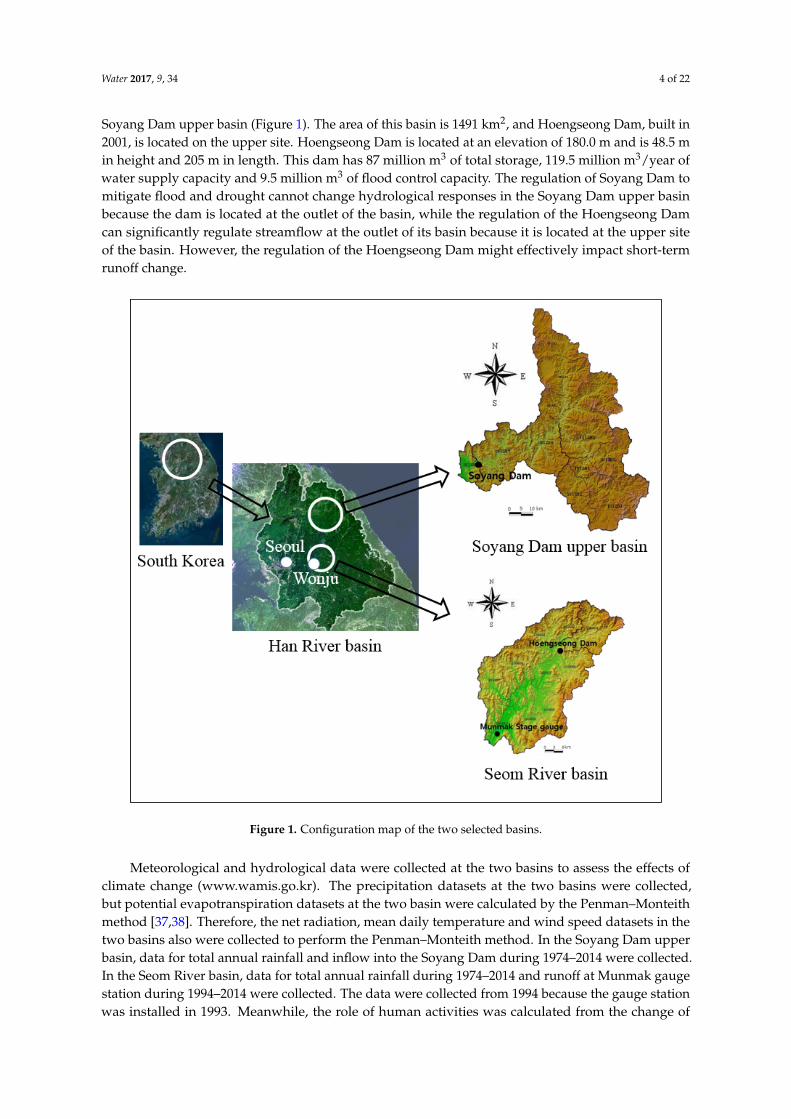
Two catchments undergoing a change in population and land use were selected to comparethe relative impacts of climate change and human activities. One was the Soyang Dam upper basin(128◦15′ E~128◦56′ E, 38◦13′ N~38◦24′ N), located in northeastern South Korea (Figure 1). Soyang Damwas constructed in 1973 and has played an important role in preventing floods and supplying water tothe area around the Korean capital, Seoul. This basin is 2703 km2 in area and consists of three sub-basins,Inbuk (923.8 km2), Naerin (1069.3 km2) and Soyang (709.9 km2). The other catchment selected wasthe Seom River basin (128◦02′ E~128◦13′ E, 37◦56′ N~37◦89′ N), located about 150 km south of the

Water 2017, 9, 34 4 of 22

Soyang Dam upper basin (Figure 1). The area of this basin is 1491 km2, and Hoengseong Dam, built in2001, is located on the upper site. Hoengseong Dam is located at an elevation of 180.0 m and is 48.5 min height and 205 m in length. This dam has 87 million m3 of total storage, 119.5 million m3/year ofwater supply capacity and 9.5 million m3 of flood control capacity. The regulation of Soyang Dam tomitigate flood and drought cannot change hydrological responses in the Soyang Dam upper basinbecause the dam is located at the outlet of the basin, while the regulation of the Hoengseong Damcan significantly regulate streamflow at the outlet of its basin because it is located at the upper siteof the basin. However, the regulation of the Hoengseong Dam might effectively impact short-termrunoff change.

Water 2017, 9, 34  4 of 21 

the Soyang Dam upper basin because the dam is located at the outlet of the basin, while the regulation 

of the Hoengseong Dam can significantly regulate streamflow at the outlet of its basin because it is 

located  at  the  upper  site  of  the  basin. However,  the  regulation  of  the Hoengseong Dam might 

effectively impact short‐term runoff change. 

 

Figure 1. Configuration map of the two selected basins. 

Meteorological and hydrological data were collected at the two basins to assess the effects of 

climate change (www.wamis.go.kr). The precipitation datasets at the two basins were collected, but 

potential  evapotranspiration datasets  at  the  two  basin were  calculated  by  the Penman–Monteith   

method [37,38]. Therefore, the net radiation, mean daily temperature and wind speed datasets in the 

two basins also were collected to perform the Penman–Monteith method. In the Soyang Dam upper 

basin, data for total annual rainfall and inflow into the Soyang Dam during 1974–2014 were collected. 

In the Seom River basin, data for total annual rainfall during 1974–2014 and runoff at Munmak gauge 

station during 1994–2014 were collected. The data were collected from 1994 because the gauge station 

was  installed  in 1993. Meanwhile,  the role of human activities was calculated  from  the change of 

population and increased impervious area due to urban development. Therefore, data for population 

growth during 1966–2011 and the area of the impervious layer during 1975–2011 were collected at 

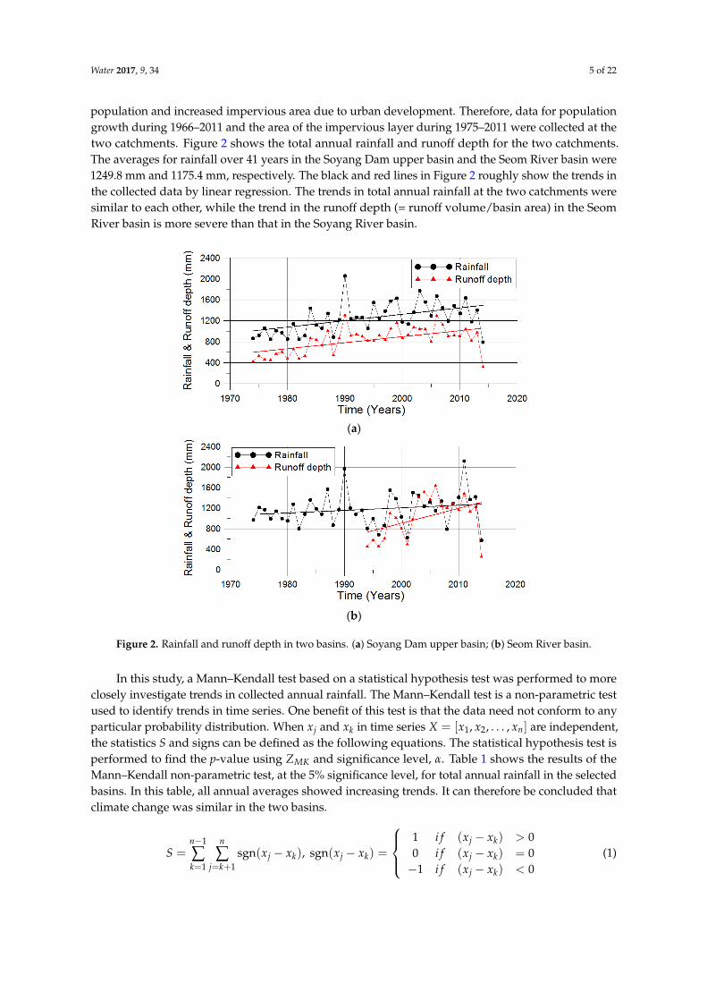
the two catchments. Figure 2 shows the total annual rainfall and runoff depth for the two catchments. 

The averages for rainfall over 41 years in the Soyang Dam upper basin and the Seom River basin were 

1249.8 mm and 1175.4 mm, respectively. The black and red lines in Figure 2 roughly show the trends 

in the collected data by linear regression. The trends in total annual rainfall at the two catchments 

were similar to each other, while the trend in the runoff depth (= runoff volume/basin area) in the 

Seom River basin is more severe than that in the Soyang River basin. 

Figure 1. Configuration map of the two selected basins.

Meteorological and hydrological data were collected at the two basins to assess the effects ofclimate change (www.wamis.go.kr). The precipitation datasets at the two basins were collected,but potential evapotranspiration datasets at the two basin were calculated by the Penman–Monteithmethod [37,38]. Therefore, the net radiation, mean daily temperature and wind speed datasets in thetwo basins also were collected to perform the Penman–Monteith method. In the Soyang Dam upperbasin, data for total annual rainfall and inflow into the Soyang Dam during 1974–2014 were collected.In the Seom River basin, data for total annual rainfall during 1974–2014 and runoff at Munmak gaugestation during 1994–2014 were collected. The data were collected from 1994 because the gauge stationwas installed in 1993. Meanwhile, the role of human activities was calculated from the change of

Water 2017, 9, 34 5 of 22

population and increased impervious area due to urban development. Therefore, data for populationgrowth during 1966–2011 and the area of the impervious layer during 1975–2011 were collected at thetwo catchments. Figure 2 shows the total annual rainfall and runoff depth for the two catchments.The averages for rainfall over 41 years in the Soyang Dam upper basin and the Seom River basin were1249.8 mm and 1175.4 mm, respectively. The black and red lines in Figure 2 roughly show the trends inthe collected data by linear regression. The trends in total annual rainfall at the two catchments weresimilar to each other, while the trend in the runoff depth (= runoff volume/basin area) in the SeomRiver basin is more severe than that in the Soyang River basin.Water 2017, 9, 34  5 of 21 

 (a) 

 (b) 

Figure 2. Rainfall and runoff depth in two basins. (a) Soyang Dam upper basin; (b) Seom River basin.   

In this study, a Mann–Kendall test based on a statistical hypothesis test was performed to more 

closely investigate trends in collected annual rainfall. The Mann–Kendall test is a non‐parametric test 

used to identify trends in time series. One benefit of this test is that the data need not conform to any 

particular  probability  distribution.  When  jx   and kx   in  time  series

1 2[ , , ..., ]nX x x x   are 

independent, the statistics  S   and signs can be defined as the following equations. The statistical 

hypothesis  test  is performed  to  find  the  p‐value using MKZ   and  significance  level,  . Table  1 

shows  the results of  the Mann–Kendall non‐parametric  test, at  the 5% significance  level,  for  total 

annual rainfall in the selected basins. In this table, all annual averages showed increasing trends. It 

can therefore be concluded that climate change was similar in the two basins. 

1

1 1

sgn( )n n

j kk j k

S x x

, 

1 ( ) 0

sgn( ) 0 ( ) 0

1 ( ) 0

j k

j k j k

j k

if x x

x x if x x

if x x

  (1) 

( 1) / [ ]

0

( 1) / [ ]

MK

S Var S

Z

S Var S

 

if

if

if

 

0

0

0

S

S

S

  (2) 

Table 1. Results of the Mann–Kendall trend test in the two basins. 

Basins  M–K Test Statistics p‐Value Decision 

Soyang Dam upper basin  3.1785  0.0015  trend 

Seom River basin  3.0252  0.0025  trend 

Figure 2. Rainfall and runoff depth in two basins. (a) Soyang Dam upper basin; (b) Seom River basin.

In this study, a Mann–Kendall test based on a statistical hypothesis test was performed to moreclosely investigate trends in collected annual rainfall. The Mann–Kendall test is a non-parametric testused to identify trends in time series. One benefit of this test is that the data need not conform to anyparticular probability distribution. When xj and xk in time series X = [x1, x2, . . . , xn] are independent,the statistics S and signs can be defined as the following equations. The statistical hypothesis test isperformed to find the p-value using ZMK and significance level, α. Table 1 shows the results of theMann–Kendall non-parametric test, at the 5% significance level, for total annual rainfall in the selectedbasins. In this table, all annual averages showed increasing trends. It can therefore be concluded thatclimate change was similar in the two basins.

S =n−1

∑k=1

n

∑j=k+1

sgn(xj − xk), sgn(xj − xk) =

10−1

i fi fi f

(xj − xk)

(xj − xk)

(xj − xk)

> 0= 0< 0

(1)

Water 2017, 9, 34 6 of 22

ZMK =

(S− 1)/

√Var[S]

0(S + 1)/

√Var[S]

i fi fi f

S > 0S = 0S < 0

(2)

Table 1. Results of the Mann–Kendall trend test in the two basins.

Basins M–K Test Statistics p-Value Decision

Soyang Dam upper basin 3.1785 0.0015 trendSeom River basin 3.0252 0.0025 trend

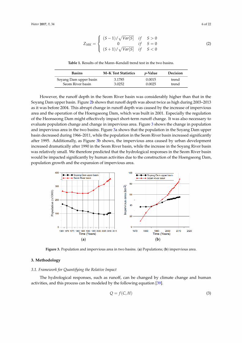
However, the runoff depth in the Seom River basin was considerably higher than that in theSoyang Dam upper basin. Figure 2b shows that runoff depth was about twice as high during 2003–2013as it was before 2004. This abrupt change in runoff depth was caused by the increase of imperviousarea and the operation of the Hoengseong Dam, which was built in 2001. Especially the regulationof the Heonseong Dam might effectively impact short-term runoff change. It was also necessary toevaluate population change and change in impervious area. Figure 3 shows the change in populationand impervious area in the two basins. Figure 3a shows that the population in the Soyang Dam upperbasin decreased during 1966–2011, while the population in the Seom River basin increased significantlyafter 1995. Additionally, as Figure 3b shows, the impervious area caused by urban developmentincreased dramatically after 1990 in the Seom River basin, while the increase in the Soyang River basinwas relatively small. We therefore predicted that the hydrological responses in the Seom River basinwould be impacted significantly by human activities due to the construction of the Hoengseong Dam,population growth and the expansion of impervious area.

Water 2017, 9, 34  6 of 21 

However, the runoff depth  in the Seom River basin was considerably higher than that  in the 

Soyang Dam  upper  basin.  Figure  2b  shows  that  runoff  depth was  about  twice  as  high  during   

2003–2013 as it was before 2004. This abrupt change in runoff depth was caused by the increase of 

impervious area and the operation of the Hoengseong Dam, which was built in 2001. Especially the 

regulation of  the Heonseong Dam might effectively  impact short‐term  runoff change.  It was also 

necessary to evaluate population change and change in impervious area. Figure 3 shows the change 

in population and  impervious area  in  the  two basins. Figure 3a shows  that  the population  in  the 

Soyang Dam upper basin decreased during 1966–2011, while the population in the Seom River basin 

increased significantly after 1995. Additionally, as Figure 3b shows, the impervious area caused by 

urban development increased dramatically after 1990 in the Seom River basin, while the increase in 

the Soyang River basin was relatively small. We therefore predicted that the hydrological responses 

in the Seom River basin would be impacted significantly by human activities due to the construction 

of the Hoengseong Dam, population growth and the expansion of impervious area. 

 (a)  (b)

Figure 3. Population and impervious area in two basins. (a) Populations; (b) impervious area. 

3. Methodology 

3.1. Framework for Quantifying the Relative Impact 

The  hydrological  responses,  such  as  runoff,  can  be  changed  by  climate  change  and  human 

activities, and this process can be modeled by the following equation [39]. 

( , )Q f C H   (3) 

Here,  Q   is  runoff;  C   and  H   are variables  to  represent  climate  change and human activities, 

respectively. Using a first‐order approximation to Equation (3), Equation (4) can be derived as [39]: 

C H

Q QQ C H Q Q

C H

  (4) 

Here,  Q   is total change in runoff; CQ   and  HQ   represent changes in runoff due to climate 

change  and  human  activities,  respectively.  Among  two  variables  ( CQ   and HQ ),  only  one 

variable needs to be identified to solve Equation (4) because total runoff change,  Q , is already a 

known  variable  from  the  observed  runoff.  Wang  et  al.  [25]  regarded  these  two  variables  as 

independent, although climate change and human activities interact with each other in the real world. 

Therefore, in this study, the independent assumption was applied to all calculating processes. 

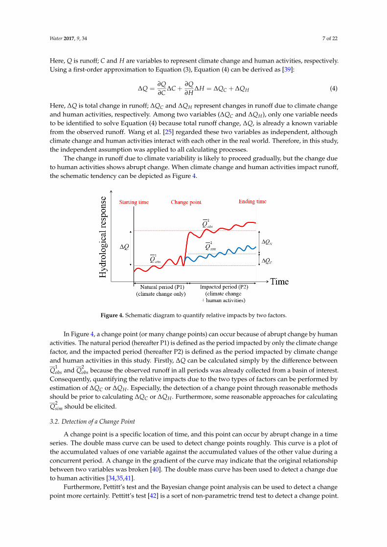
The change in runoff due to climate variability is likely to proceed gradually, but the change due 

to human activities shows abrupt change. When climate change and human activities impact runoff, 

the schematic tendency can be depicted as Figure 4. 

Figure 3. Population and impervious area in two basins. (a) Populations; (b) impervious area.

3. Methodology

3.1. Framework for Quantifying the Relative Impact

The hydrological responses, such as runoff, can be changed by climate change and humanactivities, and this process can be modeled by the following equation [39].

Q = f (C, H) (3)

Water 2017, 9, 34 7 of 22

Here, Q is runoff; C and H are variables to represent climate change and human activities, respectively.Using a first-order approximation to Equation (3), Equation (4) can be derived as [39]:

∆Q =∂Q∂C

∆C +∂Q∂H

∆H = ∆QC + ∆QH (4)

Here, ∆Q is total change in runoff; ∆QC and ∆QH represent changes in runoff due to climate changeand human activities, respectively. Among two variables (∆QC and ∆QH), only one variable needsto be identified to solve Equation (4) because total runoff change, ∆Q, is already a known variablefrom the observed runoff. Wang et al. [25] regarded these two variables as independent, althoughclimate change and human activities interact with each other in the real world. Therefore, in this study,the independent assumption was applied to all calculating processes.

The change in runoff due to climate variability is likely to proceed gradually, but the change dueto human activities shows abrupt change. When climate change and human activities impact runoff,the schematic tendency can be depicted as Figure 4.Water 2017, 9, 34  7 of 21 

 

Figure 4. Schematic diagram to quantify relative impacts by two factors. 

In Figure 4, a change point  (or many change points) can occur because of abrupt change by 

human activities. The natural period  (hereafter P1)  is defined as  the period  impacted by only  the 

climate change factor, and the impacted period (hereafter P2) is defined as the period impacted by 

climate  change and human activities  in  this  study. Firstly,  Q   can be  calculated  simply by  the 

difference between 1

obsQ   and 2

obsQ   because the observed runoff in all periods was already collected 

from a basin of interest. Consequently, quantifying the relative impacts due to the two types of factors 

can  be  performed  by  estimation  of  CQ   or HQ .  Especially,  the  detection  of  a  change  point 

through  reasonable methods  should  be  prior  to  calculating CQ   or 

HQ .  Furthermore,  some 

reasonable approaches for calculating 2

simQ   should be elicited. 

3.2. Detection of a Change Point 

A change point is a specific location of time, and this point can occur by abrupt change in a time 

series. The double mass curve can be used to detect change points roughly. This curve is a plot of the 

accumulated  values  of  one  variable  against  the  accumulated  values  of  the  other  value during  a 

concurrent period. A change in the gradient of the curve may indicate that the original relationship 

between two variables was broken [40]. The double mass curve has been used to detect a change due 

to human activities [34,35,41].   

Furthermore, Pettitt’s test and the Bayesian change point analysis can be used to detect a change 

point more certainly. Pettitt’s test [42] is a sort of non‐parametric trend test to detect a change point. 

This test is commonly applied to detect a single change point in hydrological or meteorological time 

series. The null hypothesis in this test is 0H : some T variables follow one or more distributions that 

have  the same  location parameter  (so, no change); and  then,  the alternative hypothesis  is AH : a 

change  point  exists  in  the  time  series.  The  non‐parametric  statistics  by  Pettitt  is  defined  as   

Equation  (5). The  change point  is detected  at TK , provided  that  the  statistics  is  significant. The 

significance probability of TK   is approximated as Equation (6). 

,maxT t TK U , ,

1 1

sgn( )t T

t T i ji j t

U x x

  (5) 

2

3 2

62 exp TKp

T T

 (6) 

Another change point test is Bayesian change point analysis (BCP analysis), and its advantage is 

to detect many change points through multiple change point analysis at once. Let us assume that 

Figure 4. Schematic diagram to quantify relative impacts by two factors.

In Figure 4, a change point (or many change points) can occur because of abrupt change by humanactivities. The natural period (hereafter P1) is defined as the period impacted by only the climate changefactor, and the impacted period (hereafter P2) is defined as the period impacted by climate changeand human activities in this study. Firstly, ∆Q can be calculated simply by the difference betweenQ1

obs and Q2obs because the observed runoff in all periods was already collected from a basin of interest.

Consequently, quantifying the relative impacts due to the two types of factors can be performed byestimation of ∆QC or ∆QH . Especially, the detection of a change point through reasonable methodsshould be prior to calculating ∆QC or ∆QH . Furthermore, some reasonable approaches for calculatingQ2

sim should be elicited.

3.2. Detection of a Change Point

A change point is a specific location of time, and this point can occur by abrupt change in a timeseries. The double mass curve can be used to detect change points roughly. This curve is a plot ofthe accumulated values of one variable against the accumulated values of the other value during aconcurrent period. A change in the gradient of the curve may indicate that the original relationshipbetween two variables was broken [40]. The double mass curve has been used to detect a change dueto human activities [34,35,41].

Furthermore, Pettitt’s test and the Bayesian change point analysis can be used to detect a changepoint more certainly. Pettitt’s test [42] is a sort of non-parametric trend test to detect a change point.

Water 2017, 9, 34 8 of 22

This test is commonly applied to detect a single change point in hydrological or meteorological timeseries. The null hypothesis in this test is H0: some T variables follow one or more distributions that havethe same location parameter (so, no change); and then, the alternative hypothesis is HA: a change pointexists in the time series. The non-parametric statistics by Pettitt is defined as Equation (5). The changepoint is detected at KT , provided that the statistics is significant. The significance probability of KT isapproximated as Equation (6).

KT = max|Ut,T |, Ut,T =t

∑i=1

T

∑j=t+1

sgn(xi − xj) (5)

p ≈ 2 exp

(−6K2

TT3 + T2

)(6)

Another change point test is Bayesian change point analysis (BCP analysis), and its advantage is todetect many change points through multiple change point analysis at once. Let us assume that {xi}i=n

i=1is a sequence of observed time series with the probability density functions p1(x), p2(x), . . . , pn(x).Therefore, for a sequence of n independent random variables X = (X1, X2, . . . , Xn), the change pointmodel can be described by Equation (7). In Equation (7), the parameter in probability density functionsθ1 6= θ2 6=, . . . , 6= θn and the change points τ1, τ2, . . . , τn−1 are unknown. Therefore, this time seriescan be divided into n homogenous groups if the locations of change points are determined. Thus,each part of the sequence of random variables is distributed as statistical distributions, which belongto the same class, but with a different unknown parameter θ, such as the mean and variance. The BCPanalysis uses the Bayesian framework to detect some change point in Equation (7).

Xi ∼

p1(x) = p(xi|θ1 ), 1 ≤ i ≤ τ1

p2(x) = p(xi|θ2 ), τ1 < i ≤ τ2...

...

pn(x) = p(xi|θn ), τn−1 < i ≤ τn

(7)

Especially, Barry and Hartigan [43] used the product partition model, which assumes that theprobability of any partition is proportional to a product of prior cohesions. Chib [44] formulatedthe multiple change point model using the Markov process with transition probabilities. Recently,the BCP analysis has been applied to detect some abrupt change in hydrological or meteorologicaltime series [45–47]. The double mass curve, Pettitt’s test and the BCP analysis were used to detect achange point in observed runoff time series in this study. Furthermore, the BCP package developed byErdman and Emerson [48] on R was used.

3.3. Generation of Simulated Runoff by the Hydrological Model

A hydrological model can be used to simulate Q2sim in Figure 4. The basic concept is that

the hydrological models simulate a condition that would have occurred without human activities,this natural condition in P1, which would be only a result of climate change factors. Therefore, it isnecessary that the selected hydrological model should be firstly calibrated on observed runoff in thenatural period, P1. After calibration to P1, the calibrated parameters in the selected hydrologicalmodel should be used to simulate runoff in the impacted period, P2. Finally, the quantitative impactdue to human activities can be calculated as Equation (8). Furthermore, it is possible to calculate thequantitative impact due to climate change, ∆QC, from Equation (4).

∆QH = Q2obs −Q2

sim (8)

Water 2017, 9, 34 9 of 22

The SWAT model was selected to simulate the runoff in P1 and P2 in this study. This model is acontinuous, semi-distributed, physically-based hydrological model developed by the U.S. Departmentof Agriculture-Agriculture Research Service (USDA-ARS). Furthermore, this model simulates theimpact of land management strategy on water, sediment and various water pollutants. The SWATmodel is performed on hydrological response units, which are sub-units of sub-basins with uniquecombinations of soil and land use characteristics. The SWAT model requires spatial data inputs,including topography, climate, land use and soil. For a further description of the theoreticalbackground, the study of Neitsch et al. [49] can be referenced. Furthermore, the ParaSol (ParameterSolution) procedure in the SWAT-CUP (SWAT-Calibration and Uncertainty Procedures) was usedto calibrate in this study automatically. Among the various algorithms such as Particle SwarmOptimization (PSO), Sequential Uncertainty FIttting-2 (SUFI-2), Markov Chain Monte Carlo (MCMC),Generalized Likelihood Uncertainty Estimation (GLUE) in the SWAT-CUP, the SUFI-2 algorithm wasused. For more detailed information on the SUFI-2 algorithm, the report of Abbaspour [50] canbe referenced.

3.4. Generation of Simulated Runoff by Hydrological Sensitivity

Hydrological sensitivity means the change in mean annual runoff in response to the change inmean annual precipitation and potential evapotranspiration (PET). Water balance can be described byrunoff, precipitation and actual evapotranspiration (AET) as Equation (9).

P = Q + AET + ∆S (9)

Here, P, Q and AET are precipitation, runoff and actual evapotranspiration during a period,respectively. Furthermore, ∆S is the change in storage in a basin. However, in a long-term period(more than about 10 years) with an annual time scale, ∆S can be neglected because its summation canbe assumed as zero [51].

Meanwhile, in an analysis of water resources’ modeling, the Budyko curve has been frequentlyused to simulate evaporation. The Budyko curve based on Budyko’s assumption [36] is developedby two balance equations on water and energy. One is Equation (9), and the other is Equation (10),to represent the energy balance in a basin [52].

N = L× AET + H + ∆G (10)

Here, N, L, H and ∆G are the net radiation, the latent heat for evaporation, the sensible heat fluxduring a period and the change of net ground heat flux, respectively. Furthermore, ∆G can be assumedas zero for the same reason as ∆S [51]. After elimination of ∆S and ∆G in Equations (9) and (10),it is assumed that PET = N/L and γ = H/(L× AET). By dividing Equation (10) by Equation (9),Equation (11) can be derived simply.

PETP

=AET

P+

AET × γ

P=

AETP

(1 + γ) = φ (11)

Here, γ and φ are called the Bowen ratio and aridity index. Because the Bowen ratio can be assumed asa function of the aridity index [51], γ = f (φ), Equation (11) can be finally rearranged as Equation (12).

AETP

=φ

1 + f (φ)= F(φ) (12)

Water 2017, 9, 34 10 of 22

Here, F(φ) is called the Budyko curve equation. Many studies have been performed to find F(φ) usingactual evapotranspiration and precipitation time series of more than 10 years on various regions. Thecommonly used 5 functions were developed by Schreiber [52], Ol’dekop [53], Pike [1], Budyko [36]and Fu [54]. The estimated functions are described in Table 2.

Table 2. Commonly-used Budyko curves.

Name of Function F(φ)

Schreiber (1904) 1− e−φ

Ol’dekop (1911) φtanh(1/φ)

Budyko (1948) [φtanh(1/φ)(1− e−φ)]0.5

Pike (1964) (1 + φ−2)−0.5

Fu (1981) 1 + φ− (1 + φ2.5)1/2.5

Therefore, the potential evapotranspiration, PET, should be estimated by Equation (11) todetermine the aridity index, φ. In this study, the evapotranspirations, PETs, in Soyang Dam upperbasin and Seom River basin were estimated by the Penman–Monteith method. After calculating thearidity index, φ, in the basin of interest, the actual evapotranspiration, AET, can be calculated by thevarious types of Budyko curves. Especially, Zhang et al. [55] developed another type of Budyko curveusing mean annual evapotranspiration to vegetation. Equation (13) is the relationship developed byZhang et al. [55].

AETP

= F(φ) =1 + ω(PET/P)

1 + ω(PET/P) + (PET/P)−1 (13)

Here, ω is a plant-available water coefficient related to vegetation type. In this study, the plant-availablewater coefficient, ω, was calibrated by the actual evapotranspiration, AET, in Equation (9).

The hydrological sensitivity, which means perturbation in runoff, ∆Q can be derived by thewater balance equation (Equation (9)). Especially, in the hydrological sensitivity approach, ∆Q canbe assumed ∆QC because ∆Q is impacted by only meteorological variables, such as precipitationand actual evapotranspiration. Therefore, ∆Q can be denoted by ∆QC in Equation (4). Finally,the perturbation of Equation (9) without human activities can be described by Equation (14).

∆QC = ∆P− ∆AET (14)

Here, ∆QC, ∆P and ∆AET are the change in runoff due to only climate change, the change inprecipitation and the change in actual evapotranspiration.

Koster and Suarez [56] developed a relationship between actual evapotranspiration and theBudyko curve function. The total derivative to Equation (12) (AET = P × F(φ)) is described asEquation (15). Furthermore, the total derivative to the aridity index function (φ = PET/P) isrepresented by Equation (16).

d(AET) = F(φ)dP + PF′(φ)dφ⇒ ∆AET = F(φ)∆P + PF′(φ)∆φ (15)

dφ =1P

d(PET)− PETP2 dP⇒ ∆φ =

1P

∆(PET)− PETP2 ∆P (16)

Water 2017, 9, 34 11 of 22

By substituting Equation (16) for Equation (15) and rearranging,

∆AET = [F(φ)− φF′(φ)]∆P + F′(φ)∆PET (17)

Furthermore, by substituting Equation (17) for Equation (14),

∆QC = [1− F(φ) + φF′(φ)]∆P− F′(φ)∆PET = α∆P + β∆PET (18)

Because Equation (9) can be rearranged by AET = P× F(φ):

Q = P(1− F(φ)) (19)

Dividing Equation (18) by Equation (19) and using P = PET/φ, Equation (20) is derived as:

∆QC =∆PP

Q(

1 +φF′(φ)

1− F(φ)

)+

∆PETPET

Q(− φF′(φ)

1− F(φ)

)= εP

∆PP

Q + εPET∆PETPET

Q (20)

Here, εP and εPET are called the elasticity coefficient of precipitation and potential evapotranspiration,and εP + εP = 1. Finally, Equation (20) can be used to estimate the change in runoff due to only climatefactors. Furthermore, in Equation (18), the coefficients α and β were estimated by Li et al. [57].

α =1 + 2x + 3ωx

(1 + x + ωx2)2 , β = − 1 + 2ωx

(1 + x + ωx2)2 (21)

Here, ω is the plant-available water coefficient in Zhang’s Budyko-based method [55], and x = PET/P.In this study, the 5 Budyko-based methods (Table 2), by calculating the elasticity coefficients, wereused. Furthermore, Zhang’s method using coefficients α and β was used.

4. Applications

4.1. Detection of Change Points over Different Time Scales

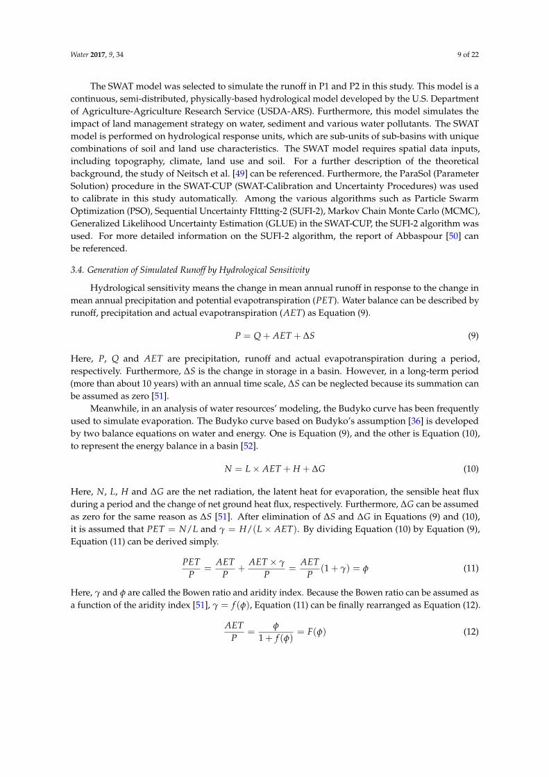
In this study, the data for daily precipitation and observed runoff depth during 1974–2014 in theSoyang Dam upper basin and the data for the same factors during 1994–2014 in the Seom River basinwere used to detect a change point. The daily data were used only at the seasonal and annual time scalesto detect change points, because change point detection at the monthly scale is very time consuming.It was therefore assumed that the monthly change points in a season were identical. The seasonal datawere divided into four sections: January–March (JFM), April–June (AMJ), July–September (JAS) andOctober–December (OND) according to the meteorological characteristics of South Korea.

Figure 5a–e shows the results obtained using the double mass curve technique in the Soyang Damupper basin. The relationship between straight lines with slightly different slopes for the Soyang Damupper basin is shown. It can therefore be concluded that the change points were located at 1987–1988(JFM), 1988–1989 (AMJ), 1982–1983 (JAS) and 1983–1984 (OND). At the annual time scale, the changepoint was located at 1983–1984. We can therefore conclude that the runoff characteristics in JFM–AMJwere different from those in JAS–OND.

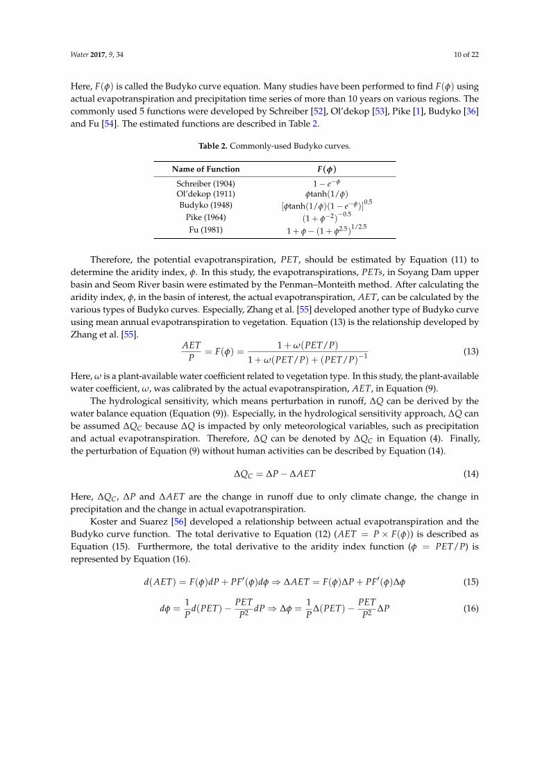
In Figure 6a–e for the Seom River basin, the slope lines were clearly changed around 2002–2003.We can conclude that the change points were located at 2000–2001 (JFM), 2002–2003 (AMJ), 2002–2003(JAS) and 2000–2001 (OND). At the annual time scale, the change point was located at 2001–2002.The change in runoff in the Seom River basin might result from the regulation of the Hoengseong Dam,built on the upper site of this basin in 2001.

Water 2017, 9, 34 12 of 22

Water 2017, 9, 34  11 of 21 

2 2

1 2 3

(1 )

x x

x x

,  2 2

1 2

(1 )

x

x x

  (21) 

Here,    is  the  plant‐available  water  coefficient  in  Zhang’s  Budyko‐based  method  [55],  and 

/x PET P .  In  this  study,  the  5 Budyko‐based methods  (Table  2),  by  calculating  the  elasticity 

coefficients, were used. Furthermore, Zhang’s method using coefficients    and   was used.   

4. Applications 

4.1. Detection of Change Points over Different Time Scales 

In this study, the data for daily precipitation and observed runoff depth during 1974–2014 in the 

Soyang Dam upper basin and the data for the same factors during 1994–2014 in the Seom River basin 

were used to detect a change point. The daily data were used only at the seasonal and annual time 

scales  to detect  change points, because  change point detection  at  the monthly  scale  is very  time 

consuming.  It was  therefore assumed  that  the monthly change points  in a  season were  identical.   

The  seasonal  data  were  divided  into  four  sections:  January–March  (JFM),  April–June  (AMJ),   

July–September (JAS) and October–December (OND) according to the meteorological characteristics 

of South Korea. 

Figure 5a–e shows the results obtained using the double mass curve technique in the Soyang 

Dam upper basin. The relationship between straight lines with slightly different slopes for the Soyang 

Dam upper basin  is shown.  It can  therefore be concluded  that  the change points were  located at   

1987–1988 (JFM), 1988–1989 (AMJ), 1982–1983 (JAS) and 1983–1984 (OND). At the annual time scale, 

the change point was located at 1983–1984. We can therefore conclude that the runoff characteristics 

in JFM–AMJ were different from those in JAS–OND. 

 (a)  (b) (c) 

 

 

(d)  (e)  

Figure  5. Detection  of  change  point  in  Soyang Dam  upper  basin  (double mass  curve).  (a)  JFM;   

(b) AMJ; (c) JAS; (d) OND; (e) annual. The numbers in figures mean years (e.g., 14 means 2014 year). 

In Figure 6a–e for the Seom River basin, the slope lines were clearly changed around 2002–2003. 

We  can  conclude  that  the  change  points  were  located  at  2000–2001  (JFM),  2002–2003  (AMJ),   

2002–2003  (JAS) and 2000–2001  (OND). At  the annual  time scale,  the change point was  located at 

2001–2002. The change  in  runoff  in  the Seom River basin might  result  from  the  regulation of  the 

Hoengseong Dam, built on the upper site of this basin in 2001. 

Figure 5. Detection of change point in Soyang Dam upper basin (double mass curve). (a) JFM; (b) AMJ;(c) JAS; (d) OND; (e) annual. The numbers in figures mean years (e.g., 14 means 2014 year).Water 2017, 9, 34  12 of 21 

 (a)  (b) (c) 

 

 

(d)  (e)  

Figure  6. Detection of  change point  in Seom River basin  (double mass  curve).  (a)  JFM;  (b) AMJ;   

(c) JAS; (d) OND; (e) annual. The numbers in figures mean years (e.g., 14 means 2014 year). 

It is very important to separate the climate change and human activities contributing to these 

results. Pettitt’s test at the 5% significance level and the BCP (Bayesian change point) analysis using 

the  posterior  mean  change  with  the  probability  of  change  were  therefore  performed  to  more 

accurately locate the change points in the two selected basins. Table 3 shows the results of Pettitt’s test, 

and Table 4 shows the results of the BCP analysis. Apparently, the results from the three techniques 

were very similar. The seasonal change points drawn from all results are summarized in Table 5. 

Table 3. Results of change point detection by Pettitt’s test under the 5% significance level. 

Seasons Soyang Dam Upper Basin Seom River Basin 

p‐Value  Change Point p‐Value Change Point 

JFM  0.0000  1988  0.0206  2001 

AMJ  0.0149  1989  0.0219  2002 

JAS  0.0007  1983  0.0134  2002 

OND  0.0005  1983  0.0362  2001 

Annual  0.0007  1984  0.0134  2002 

Table 4. Results of change point detection by the Bayesian change point (BCP) analysis. 

Seasons Soyang Dam Upper Basin Seom River Basin 

Probability of Change  Change Point Probability of Change Change Point

JFM  0.887  1988  0.982  2001 

AMJ  0.668  1989  0.954  2003 

JAS  0.888  1983  0.987  2002 

OND  0.914  1984  0.944  2001 

Annual  0.528  1983  0.897  2002 

Table 5. Results of final change point in two basins. 

Seasons Final Change Point

Soyang Dam Upper Basin Seom River Basin 

JFM  1988  2001 

AMJ  1989  2003 

JAS  1983  2002 

OND  1984  2001 

Annual  1983  2002 

Figure 6. Detection of change point in Seom River basin (double mass curve). (a) JFM; (b) AMJ; (c) JAS;(d) OND; (e) annual. The numbers in figures mean years (e.g., 14 means 2014 year).

It is very important to separate the climate change and human activities contributing to theseresults. Pettitt’s test at the 5% significance level and the BCP (Bayesian change point) analysis usingthe posterior mean change with the probability of change were therefore performed to more accuratelylocate the change points in the two selected basins. Table 3 shows the results of Pettitt’s test, and Table 4shows the results of the BCP analysis. Apparently, the results from the three techniques were verysimilar. The seasonal change points drawn from all results are summarized in Table 5.

Water 2017, 9, 34 13 of 22

Table 3. Results of change point detection by Pettitt’s test under the 5% significance level.

SeasonsSoyang Dam Upper Basin Seom River Basin

p-Value Change Point p-Value Change Point

JFM 0.0000 1988 0.0206 2001AMJ 0.0149 1989 0.0219 2002JAS 0.0007 1983 0.0134 2002

OND 0.0005 1983 0.0362 2001Annual 0.0007 1984 0.0134 2002

Table 4. Results of change point detection by the Bayesian change point (BCP) analysis.

SeasonsSoyang Dam Upper Basin Seom River Basin

Probability of Change Change Point Probability of Change Change Point

JFM 0.887 1988 0.982 2001AMJ 0.668 1989 0.954 2003JAS 0.888 1983 0.987 2002

OND 0.914 1984 0.944 2001Annual 0.528 1983 0.897 2002

Table 5. Results of final change point in two basins.

SeasonsFinal Change Point

Soyang Dam Upper Basin Seom River Basin

JFM 1988 2001AMJ 1989 2003JAS 1983 2002

OND 1984 2001Annual 1983 2002

4.2. Calibration and Verification of the SWAT Model

The two approaches, the hydrological model method and the hydrological sensitivity method,were used to quantify the relative impacts of climate change and human activities in the two basins.The SWAT models were developed for the selected basins to simulate the runoff during the impactedperiod, P2. It is therefore necessary to calibrate and validate the SWAT models during the naturalperiod, P1. Additionally, the calibration should be performed for two distinct periods in the SoyangDam upper basin because the change points in JFM–AMJ and those in JAS-annual were different.

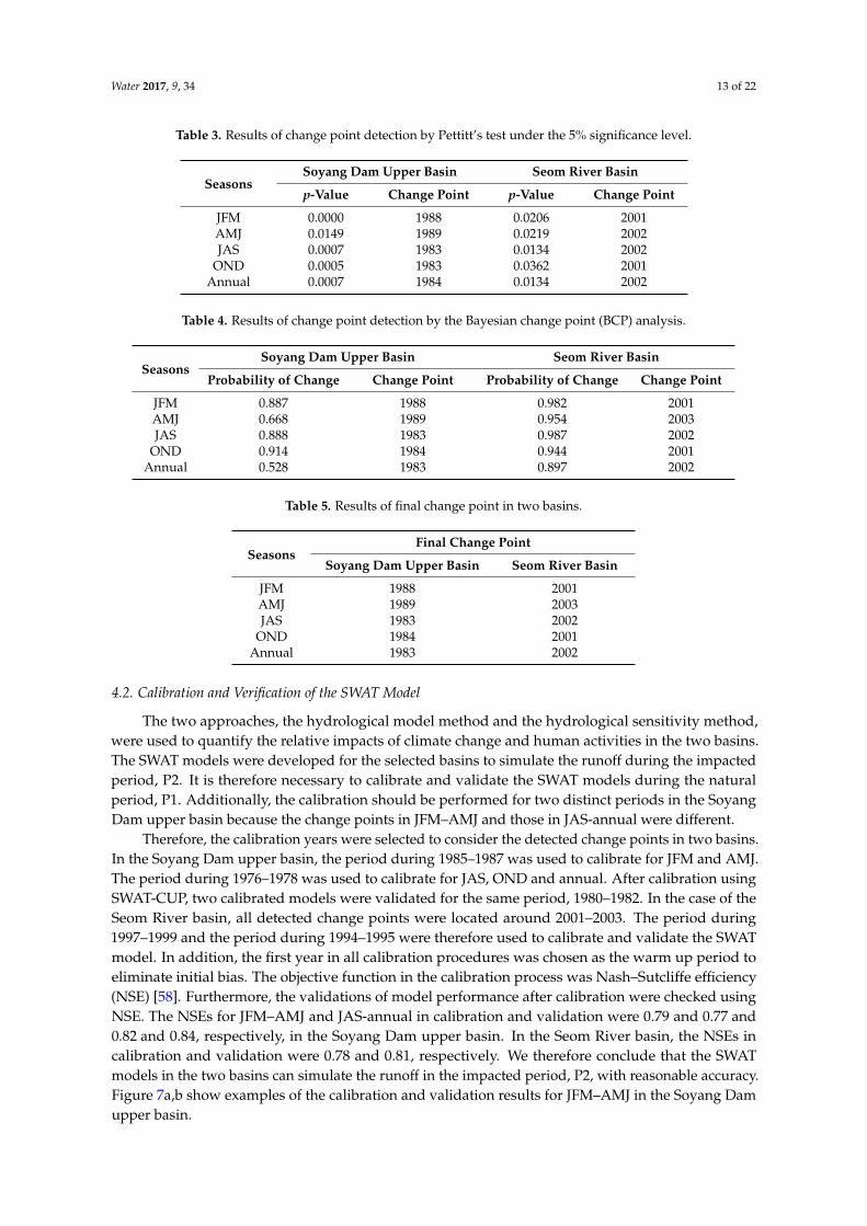
Therefore, the calibration years were selected to consider the detected change points in two basins.In the Soyang Dam upper basin, the period during 1985–1987 was used to calibrate for JFM and AMJ.The period during 1976–1978 was used to calibrate for JAS, OND and annual. After calibration usingSWAT-CUP, two calibrated models were validated for the same period, 1980–1982. In the case of theSeom River basin, all detected change points were located around 2001–2003. The period during1997–1999 and the period during 1994–1995 were therefore used to calibrate and validate the SWATmodel. In addition, the first year in all calibration procedures was chosen as the warm up period toeliminate initial bias. The objective function in the calibration process was Nash–Sutcliffe efficiency(NSE) [58]. Furthermore, the validations of model performance after calibration were checked usingNSE. The NSEs for JFM–AMJ and JAS-annual in calibration and validation were 0.79 and 0.77 and0.82 and 0.84, respectively, in the Soyang Dam upper basin. In the Seom River basin, the NSEs incalibration and validation were 0.78 and 0.81, respectively. We therefore conclude that the SWATmodels in the two basins can simulate the runoff in the impacted period, P2, with reasonable accuracy.Figure 7a,b show examples of the calibration and validation results for JFM–AMJ in the Soyang Damupper basin.

Water 2017, 9, 34 14 of 22

Water 2017, 9, 34  13 of 21 

4.2. Calibration and Verification of the SWAT Model 

The two approaches, the hydrological model method and the hydrological sensitivity method, 

were used to quantify the relative impacts of climate change and human activities in the two basins. 

The SWAT models were developed for the selected basins to simulate the runoff during the impacted 

period, P2. It is therefore necessary to calibrate and validate the SWAT models during the natural 

period, P1. Additionally, the calibration should be performed for two distinct periods in the Soyang 

Dam upper basin because the change points in JFM–AMJ and those in JAS‐annual were different. 

Therefore,  the  calibration years were  selected  to  consider  the detected  change points  in  two 

basins. In the Soyang Dam upper basin, the period during 1985–1987 was used to calibrate for JFM 

and AMJ.  The  period  during  1976–1978 was  used  to  calibrate  for  JAS, OND  and  annual. After 

calibration using SWAT‐CUP, two calibrated models were validated for the same period, 1980–1982. 

In the case of the Seom River basin, all detected change points were located around 2001–2003. The 

period during  1997–1999  and  the  period during  1994–1995 were  therefore  used  to  calibrate  and 

validate the SWAT model. In addition, the first year in all calibration procedures was chosen as the 

warm  up  period  to  eliminate  initial  bias.  The  objective  function  in  the  calibration  process was   

Nash–Sutcliffe  efficiency  (NSE)  [58].  Furthermore,  the  validations  of  model  performance  after 

calibration were  checked using NSE. The NSEs  for  JFM–AMJ  and  JAS‐annual  in  calibration  and 

validation were 0.79 and 0.77 and 0.82 and 0.84, respectively, in the Soyang Dam upper basin. In the 

Seom  River  basin,  the NSEs  in  calibration  and  validation were  0.78  and  0.81,  respectively. We 

therefore conclude that the SWAT models in the two basins can simulate the runoff in the impacted 

period, P2, with reasonable accuracy. Figure 7a,b show examples of the calibration and validation 

results for JFM–AMJ in the Soyang Dam upper basin. 

 (a) 

 (b) 

Figure 7. Calibration and validation of  the Soil and Water Assessment Tool  (SWAT) model  in  the 

Soyang Dam upper basin. (a) Calibration on JFM and AMJ; (b) validation on JFM and AMJ. Figure 7. Calibration and validation of the Soil and Water Assessment Tool (SWAT) model in theSoyang Dam upper basin. (a) Calibration on JFM and AMJ; (b) validation on JFM and AMJ.

4.3. Verification of the Hydrological Model Approach

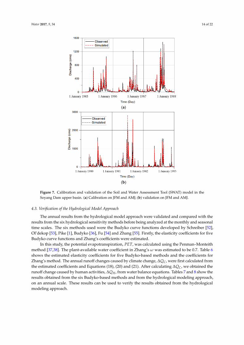
The annual results from the hydrological model approach were validated and compared with theresults from the six hydrological sensitivity methods before being analyzed at the monthly and seasonaltime scales. The six methods used were the Budyko curve functions developed by Schreiber [52],Ol’dekop [53], Pike [1], Budyko [36], Fu [54] and Zhang [55]. Firstly, the elasticity coefficients for fiveBudyko curve functions and Zhang’s coefficients were estimated.

In this study, the potential evapotranspiration, PET, was calculated using the Penman–Monteithmethod [37,38]. The plant-available water coefficient in Zhang’s ω was estimated to be 0.7. Table 6shows the estimated elasticity coefficients for five Budyko-based methods and the coefficients forZhang’s method. The annual runoff changes caused by climate change, ∆QC, were first calculated fromthe estimated coefficients and Equations (18), (20) and (21). After calculating ∆QC, we obtained therunoff change caused by human activities, ∆QH , from water balance equations. Tables 7 and 8 show theresults obtained from the six Budyko-based methods and from the hydrological modeling approach,on an annual scale. These results can be used to verify the results obtained from the hydrologicalmodeling approach.

Water 2017, 9, 34 15 of 22

Table 6. Estimated value of elasticity coefficients and Zhang’s coefficients.

ElasticityCoefficients

Schreiber(1904)

Ol’dekop(1911)

Budyko(1948)

Pike(1964)

Fu(1981)

Zhang (2001)(α and β)

εP 1.6688 2.0690 2.4570 1.8649 1.7875 1.1307εPET −0.6688 −1.0690 −1.4570 −0.8649 −0.7875 −0.6523

Table 7. Verification of the hydrological modeling approach (Soyang Dam upper basin).

Items SWAT Model Schreiber Ol’dekop Budyko Pike Fu Zhang Average

∆Q (mm/year) 526.0 526.0 526.0 526.0 526.0 526.0 526.0 526.0∆QH (mm/year) 150.1 178.3 152.1 126.8 165.5 170.6 182.8 162.7∆QC (mm/year) 376.0 347.6 373.8 399.2 360.5 355.4 343.2 363.3

∆QH (%) 28.5 33.9 28.9 24.1 31.5 32.4 34.7 30.9∆QC (%) 71.5 66.1 71.1 75.9 68.5 67.6 65.3 69.1

Table 8. Verification of the hydrological modeling approach (Seom River basin).

Items SWAT Model Schreiber Ol’dekop Budyko Pike Fu Zhang Average

∆Q (mm/year) 214.0 214.0 214.0 214.0 214.0 214.0 214.0 214.0∆QH (mm/year) 154.9 158.4 154.3 150.4 156.4 157.2 160.9 156.3∆QC (mm/year) 59.0 55.6 59.8 63.7 57.7 56.8 53.1 57.8

∆QH (%) 72.4 74.0 72.1 70.2 73.1 73.5 75.2 73.0∆QC (%) 27.6 26.0 27.9 29.8 26.9 26.5 24.8 27.0

In the Soyang Dam upper basin (Table 7), the average of ∆QC calculated from the sixBudyko-based methods (69.1%) was very similar to ∆QC calculated from the hydrological modelingapproach (71.5%). In the Seom River basin (Table 8), the average of ∆QC calculated from the sixBudyko-based methods (27.0%) and ∆QC calculated from the hydrological modeling approach (27.6%)were also very similar. It can therefore be concluded that the results obtained from the hydrologicalmodeling approach over different time scales were reasonable accurate for the two basins.

4.4. Results over Different Time Scales Obtained Using Hydrological Modeling

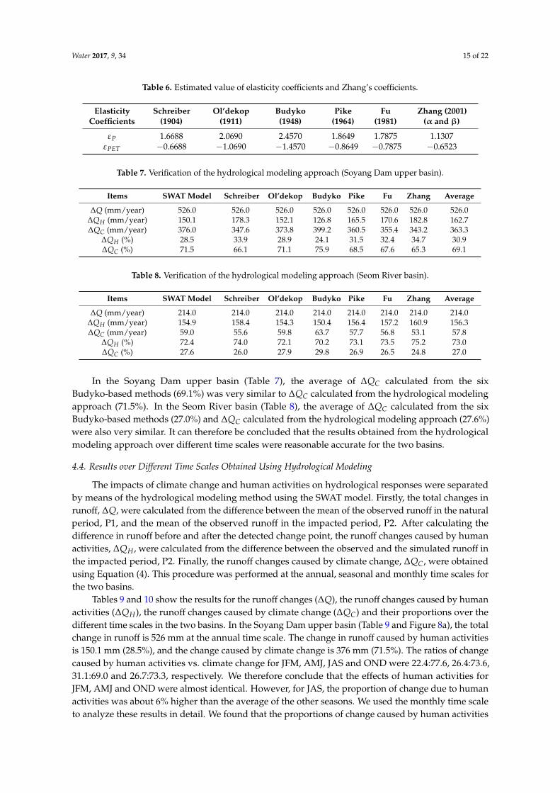
The impacts of climate change and human activities on hydrological responses were separatedby means of the hydrological modeling method using the SWAT model. Firstly, the total changes inrunoff, ∆Q, were calculated from the difference between the mean of the observed runoff in the naturalperiod, P1, and the mean of the observed runoff in the impacted period, P2. After calculating thedifference in runoff before and after the detected change point, the runoff changes caused by humanactivities, ∆QH , were calculated from the difference between the observed and the simulated runoff inthe impacted period, P2. Finally, the runoff changes caused by climate change, ∆QC, were obtainedusing Equation (4). This procedure was performed at the annual, seasonal and monthly time scales forthe two basins.

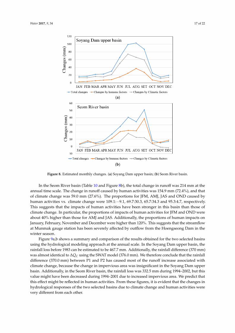
Tables 9 and 10 show the results for the runoff changes (∆Q), the runoff changes caused by humanactivities (∆QH), the runoff changes caused by climate change (∆QC) and their proportions over thedifferent time scales in the two basins. In the Soyang Dam upper basin (Table 9 and Figure 8a), the totalchange in runoff is 526 mm at the annual time scale. The change in runoff caused by human activitiesis 150.1 mm (28.5%), and the change caused by climate change is 376 mm (71.5%). The ratios of changecaused by human activities vs. climate change for JFM, AMJ, JAS and OND were 22.4:77.6, 26.4:73.6,31.1:69.0 and 26.7:73.3, respectively. We therefore conclude that the effects of human activities forJFM, AMJ and OND were almost identical. However, for JAS, the proportion of change due to humanactivities was about 6% higher than the average of the other seasons. We used the monthly time scaleto analyze these results in detail. We found that the proportions of change caused by human activities

Water 2017, 9, 34 16 of 22

were slightly higher in AUG and SEP than in other months (Figure 8a). We therefore suggest that therunoff in summer has increased slightly due to deforestation for the development of vegetable farmsin the mountains and a slight enlargement of the impervious layer. Finally, our results suggest thatthe impacts of climate change have been stronger than those of human activities in the Soyang Damupper basin.

Table 9. Quantitative impacts due to two factors (Soyang Dam upper basin).

Time Scales ∆Q (mm) ∆QH (mm) ∆QC (mm) ∆QH (%) ∆QC (%)

January 17.0 3.2 13.8 18.8 81.2February 17.2 3.8 13.4 22.1 77.9

March 22.1 5.6 16.5 25.4 74.6April 22.8 7.3 15.5 31.9 68.1May 30.5 8.7 21.8 28.5 71.5June 66.1 15.6 50.5 23.6 76.4July 99.3 24.8 74.5 25.0 75.0

August 103.3 37.3 66.0 36.1 63.9September 87.4 27.7 59.7 31.7 68.3

October 25.8 7.4 18.4 28.7 71.3November 15.2 3.6 11.6 23.7 76.3December 19.4 5.1 14.3 26.3 73.7

JFM 56.3 12.6 43.7 22.4 77.6AMJ 119.4 31.6 87.8 26.4 73.6JAS 290.0 89.8 200.2 31.0 69.0

OND 60.4 16.1 44.3 26.7 73.3Annual 526.1 150.1 376.0 28.5 71.5

Table 10. Quantitative impacts due to two factors (Seom River basin).

Time Scales ∆Q (mm) ∆QH (mm) ∆QC (mm) ∆QH (%) ∆QC (%)

January 2.8 3.7 −0.9 130.9 −30.9February 6.2 7.9 −1.7 127.2 −27.2

March 5.1 3.8 1.3 74.9 25.1April 8.2 5.0 3.2 60.9 39.1May 17.4 11.5 5.9 66.3 33.7June 27.8 20.7 7.1 74.5 25.5July 40.6 22.4 18.2 55.2 44.8

August 34.4 21.7 12.7 63.1 36.9September 51.0 38.7 12.3 75.9 24.1

October 8.4 4.7 3.7 55.7 44.3November 5.1 6.1 −1.0 120.4 −20.4December 7.0 8.7 −1.7 125.1 −25.1

JFM 14.1 15.4 −1.3 109.1 −9.1AMJ 53.4 37.2 16.2 69.7 30.3JAS 126.0 82.8 43.2 65.7 34.3

OND 20.5 19.5 1.0 95.3 4.7Annual 214.0 154.9 59.1 72.4 27.6

Water 2017, 9, 34 17 of 22

Water 2017, 9, 34  16 of 21 

change. In particular, the proportions of impacts of human activities for JFM and OND were about 

40% higher than those for AMJ and JAS. Additionally, the proportions of human impacts on January, 

February, November and December were higher  than 120%. This suggests  that  the streamflow at 

Munmak gauge  station has been  severely affected by outflow  from  the Hoengseong Dam  in  the 

winter season. 

Table 10. Quantitative impacts due to two factors (Seom River basin). 

Time Scales  Q   (mm) HQ   (mm) 

CQ   (mm)  HQ(%) 

CQ   (%) 

January  2.8  3.7  −0.9  130.9  −30.9 

February  6.2  7.9  −1.7  127.2  −27.2 

March  5.1  3.8  1.3  74.9  25.1 

April  8.2  5.0  3.2  60.9  39.1 

May  17.4  11.5  5.9  66.3  33.7 

June  27.8  20.7  7.1  74.5  25.5 

July  40.6  22.4  18.2  55.2  44.8 

August  34.4  21.7  12.7  63.1  36.9 

September  51.0  38.7  12.3  75.9  24.1 

October  8.4  4.7  3.7  55.7  44.3 

November  5.1  6.1  −1.0  120.4  −20.4 

December  7.0  8.7  −1.7  125.1  −25.1 

JFM  14.1  15.4  −1.3  109.1  −9.1 

AMJ  53.4  37.2  16.2  69.7  30.3 

JAS  126.0  82.8  43.2  65.7  34.3 

OND  20.5  19.5  1.0  95.3  4.7 

Annual  214.0  154.9  59.1  72.4  27.6 

 (a) 

 (b) 

Figure 8. Estimated monthly changes. (a) Soyang Dam upper basin; (b) Seom River basin. Figure 8. Estimated monthly changes. (a) Soyang Dam upper basin; (b) Seom River basin.

In the Seom River basin (Table 10 and Figure 8b), the total change in runoff was 214 mm at theannual time scale. The change in runoff caused by human activities was 154.9 mm (72.4%), and thatof climate change was 59.0 mm (27.6%). The proportions for JFM, AMJ, JAS and OND caused byhuman activities vs. climate change were 109.1:−9.1, 69.7:30.3, 65.7:34.3 and 95.3:4.7, respectively.This suggests that the impacts of human activities have been stronger in this basin than those ofclimate change. In particular, the proportions of impacts of human activities for JFM and OND wereabout 40% higher than those for AMJ and JAS. Additionally, the proportions of human impacts onJanuary, February, November and December were higher than 120%. This suggests that the streamflowat Munmak gauge station has been severely affected by outflow from the Hoengseong Dam in thewinter season.

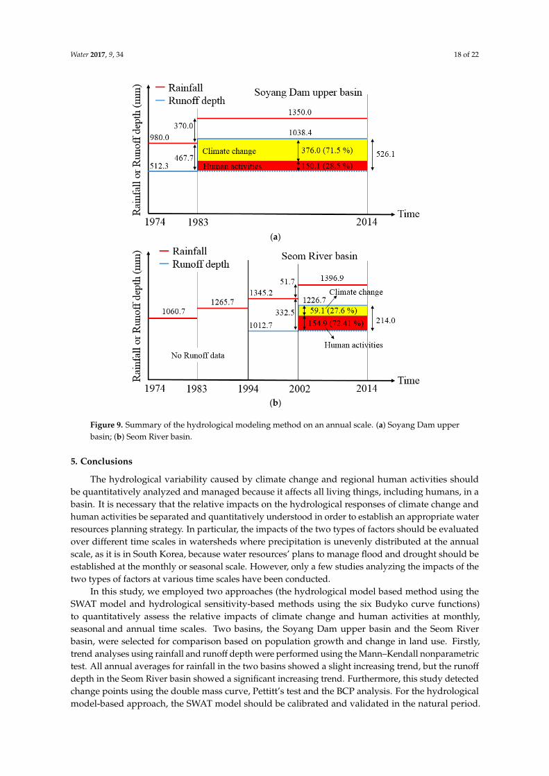
Figure 9a,b shows a summary and comparison of the results obtained for the two selected basinsusing the hydrological modeling approach at the annual scale. In the Soyang Dam upper basin, therainfall loss before 1983 can be estimated to be 467.7 mm. Additionally, the rainfall difference (370 mm)was almost identical to ∆QC using the SWAT model (376.0 mm). We therefore conclude that the rainfalldifference (370.0 mm) between P1 and P2 has caused most of the runoff increase associated withclimate change, because the change in impervious area was insignificant in the Soyang Dam upperbasin. Additionally, in the Seom River basin, the rainfall loss was 332.5 mm during 1994–2002, but thisvalue might have been decreased during 1994–2001 due to increased impervious area. We predict thatthis effect might be reflected in human activities. From these figures, it is evident that the changes inhydrological responses of the two selected basins due to climate change and human activities werevery different from each other.

Water 2017, 9, 34 18 of 22

Water 2017, 9, 34  17 of 21 

Figure 9a,b shows a summary and comparison of the results obtained for the two selected basins 

using  the hydrological modeling  approach  at  the  annual  scale.  In  the Soyang Dam upper basin,   

the rainfall  loss before 1983 can be estimated to be 467.7 mm. Additionally, the rainfall difference   

(370 mm) was almost identical to CQ   using the SWAT model (376.0 mm). We therefore conclude 

that  the rainfall difference  (370.0 mm) between P1 and P2 has caused most of  the runoff  increase 

associated with  climate  change,  because  the  change  in  impervious  area was  insignificant  in  the 

Soyang Dam upper basin. Additionally,  in  the Seom River basin,  the  rainfall  loss was 332.5 mm 

during  1994–2002, but  this value might have been decreased during  1994–2001 due  to  increased 

impervious area. We predict that this effect might be reflected in human activities. From these figures, 

it  is evident  that  the changes  in hydrological  responses of  the  two selected basins due  to climate 

change and human activities were very different from each other. 

 (a) 

 (b) 

Figure 9. Summary of the hydrological modeling method on an annual scale. (a) Soyang Dam upper 

basin; (b) Seom River basin. 

5. Conclusions 

The hydrological variability caused by climate change and regional human activities should be 

quantitatively analyzed and managed because  it affects all  living  things,  including humans,  in a 

basin. It is necessary that the relative impacts on the hydrological responses of climate change and 

human activities be separated and quantitatively understood  in order  to establish an appropriate 

water resources planning strategy. In particular, the impacts of the two types of factors should be 

evaluated over different time scales in watersheds where precipitation is unevenly distributed at the 

annual scale, as it is in South Korea, because water resources’ plans to manage flood and drought 

should be established at the monthly or seasonal scale. However, only a few studies analyzing the 

impacts of the two types of factors at various time scales have been conducted. 

Figure 9. Summary of the hydrological modeling method on an annual scale. (a) Soyang Dam upperbasin; (b) Seom River basin.

5. Conclusions

The hydrological variability caused by climate change and regional human activities shouldbe quantitatively analyzed and managed because it affects all living things, including humans, in abasin. It is necessary that the relative impacts on the hydrological responses of climate change andhuman activities be separated and quantitatively understood in order to establish an appropriate waterresources planning strategy. In particular, the impacts of the two types of factors should be evaluatedover different time scales in watersheds where precipitation is unevenly distributed at the annualscale, as it is in South Korea, because water resources’ plans to manage flood and drought should beestablished at the monthly or seasonal scale. However, only a few studies analyzing the impacts of thetwo types of factors at various time scales have been conducted.

In this study, we employed two approaches (the hydrological model based method using theSWAT model and hydrological sensitivity-based methods using the six Budyko curve functions)to quantitatively assess the relative impacts of climate change and human activities at monthly,seasonal and annual time scales. Two basins, the Soyang Dam upper basin and the Seom Riverbasin, were selected for comparison based on population growth and change in land use. Firstly,trend analyses using rainfall and runoff depth were performed using the Mann–Kendall nonparametrictest. All annual averages for rainfall in the two basins showed a slight increasing trend, but the runoffdepth in the Seom River basin showed a significant increasing trend. Furthermore, this study detectedchange points using the double mass curve, Pettitt’s test and the BCP analysis. For the hydrologicalmodel-based approach, the SWAT model should be calibrated and validated in the natural period.

Water 2017, 9, 34 19 of 22

After calibration, the annual results obtained from the hydrological model method were validatedusing the results from the six hydrological sensitivity methods. The six Budyko functions developedby Schreiber, Ol’dekop, Pike, Budyko, Fu and Zhang were used to estimate the changes caused byclimate change.

We concluded that the results obtained from the hydrological modeling approach at the differenttime scales were reasonably accurate for the two basins. The results obtained from the hydrologicalmodel method at the monthly, seasonal and annual time scales were therefore used to identify thecauses of change in the two basins. In the Soyang Dam upper basin, the change in runoff caused byhuman activities is 28.5%, and that caused by climate change is 71.5%, at the annual scale. We alsofound that the proportion of change due to human activities for JAS was slightly higher than theaverage of the proportions for other seasons. Through monthly analysis, it can be shown that theproportions for AUG and SEP were slightly higher than for other months. In the Seom River basin,the change in runoff caused by human activities is 72.4%, and that caused by climate change is 27.6%.Additionally, the proportions of change caused by human activities for the winter seasons (JFM andOND) were significantly higher than for other seasons. In particular, the proportions of change causedby human activities for JAN, FEB, NOV and DEC were higher than 120%. Finally, our results suggestthat the impacts of climate change have been stronger than those of human activities in the SoyangDam upper basin, while the impacts of human activities have been stronger than those of climatechange in the Seom River basin due to the increase of impervious area in the long-term aspect andregulation of the Hoengseong Dam in the short-term aspect.

In this study, we performed a quantitative assessment of the impacts of climate change andhuman activities on hydrological responses in two basins in South Korea. The causes of changeidentified in the two basins were significantly different. The procedure used in this study can be usedas a reference for regional water resources planning and management on monthly and seasonal timescales. In the future, the uncertainty analysis in this procedure should be performed to establish moreeffective strategies for water resources’ management. The detailed analysis related to flood and lowflow characteristics using water cycle components should be performed, and also, the independentassumption for two factors in this study should be revised to identify the interaction between climatechange and human activities in future work.

Acknowledgments: This research was supported by Basic Science Research Program through the NationalResearch Foundation (NRF) of Korea funded by the Ministry of Education (2014R1A1A2053328) and a grant(11-TI-C06) from the Advanced Water Management Research Program funded by the Ministry of Land,Infrastructure and Transport of the Korean government.

Author Contributions: Sangho Lee established the research direction and gave constructive suggestions.Sang Ug Kim performed the analysis in this study and also wrote the manuscript.

Conflicts of Interest: The authors declare no conflict of interest.

References

1. Pike, J.G. The estimation of annual runoff from meteorological data in a tropical climate. J. Hydrol. 1964, 2,116–123. [CrossRef]

2. Nash, L.L.; Gleick, P.H. Sensitivity of streamflow in the Colorado basin to climatic changes. J. Hydrol. 1991,125, 221–241. [CrossRef]

3. Burn, D.H. Hydrologic effects of climatic change in West Central Canada. J. Hydrol. 1994, 160, 53–70.[CrossRef]

4. Dam, J.C. Impacts of Climate Change and Variability on Hydrological Regimes; Cambridge University Press:Cambridge, UK, 1999.

5. Abdul Aziz, O.I.; Burn, D.H.T. Trends and variability in the hydrological regime of the Mackenzie Riverbasin. J. Hydrol. 2006, 319, 282–294. [CrossRef]

6. Li, Z.L.; Xu, Z.X.; Li, J.Y.; Li, Z.J. Shift trend and step changes for runoff time series in the Shiyang Riverbasin, northwest China. Hydrol. Process. 2008, 22, 4639–4646. [CrossRef]

Water 2017, 9, 34 20 of 22

7. Shehadeh, N.; Ananbeh, S. The impact of climate change upon winter rainfall. Am. J. Environ. Sci. 2013, 9,73–81. [CrossRef]

8. Akurut, M.; Willems, P.; Niwagaba, C.B. Potential impacts of climate change on precipitation over LakeVictoria, East Africa, in the 21st Century. Water 2014, 6, 2634–2659. [CrossRef]

9. Li, F.; Zhang, G.; Xu, Y.J. Assessing climate change impacts on water resources in the Songhua River basin.Water 2016, 8, 420. [CrossRef]

10. Labat, D.; Godderis, Y.; Probst, J.L. Evidence for global runoff increase related to climate warming.Adv. Water Resour. 2004, 27, 631–642. [CrossRef]

11. Milly, P.C.D.; Wetherhald, R.T.; Dunne, K.A.; Delworth, T.L. Increasing risk of great floods in a changingclimate. Nature 2002, 415, 514–517. [CrossRef] [PubMed]

12. Merz, B.; Vorogushyn, S.; Uhlemann, S.; Delgado, J.; Hundecha, Y. More efforts and scientific rigour areneeded to attribute trends in flood time series. Hydrol. Earth Syst. Sci. 2012, 16, 1379–1387. [CrossRef]

13. Petrow, T.; Merz, B. Trends in flood magnitude, frequency and seasonality in Germany in the period1951–2002. J. Hydrol. 2009, 371, 129–141. [CrossRef]

14. Mundelsee, M.; Börngen, M.; Tetzlaff, G.; Grünewald, U. No upward trends in the occurrence of extremefloods in central Europe. Nature 2003, 425, 166–169. [CrossRef] [PubMed]

15. Tuteja, N.K.; Vase, J.; Teng, J.; Mutendeudzi, M. Partitioning the effects of pine plantations and climatevariability on runoff from a large catchment in southeastern Australia. Water Resour. Res. 2007, 43, w08415.[CrossRef]

16. Cheng, S.J.; Wang, R.Y. An approach for evaluating the hydrological effects of urbanization and its application.Hydrol. Process. 2002, 16, 1403–1418. [CrossRef]

17. Dietz, M.E.; Clausen, J.C. Stromwater runoff and export changes with development in a traditional and lowimpact subdivision. J. Environ. Manag. 2008, 87, 560–566. [CrossRef] [PubMed]

18. Du, J.; Qian, L.; Rui, H.; Zuo, T.; Zheng, D.; Xu, Y.; Xu, C.Y. Assessing the effects of urbanization on annualrunoff and flood events using an integrated hydrological modeling system for Qinhuai River basin, China.J. Hydrol. 2012, 464–465, 127–139. [CrossRef]

19. Li, Y.; Liu, C.; Zhang, D.; Liang, K.; Li, X.; Dong, G. Reduced runoff due to anthropogenic intervention in theLoess Plateau, China. Water 2016, 8, 458. [CrossRef]

20. Seyoum, W.M.; Milewski, A.M.; Durham, M.C. Understanding the relative impacts of natural processes andhuman activities on the hydrology of the Central Rift Valley lakes, East Africa. Hydrol. Process. 2015, 29,4312–4324. [CrossRef]

21. Liu, D.; Chen, X.; Lian, Y.; Lou, Z. Impacts of climate change and human activities on surface runoff in theDongjiang River basin of China. Hydrol. Process. 2010, 24, 1487–1495. [CrossRef]

22. Jiang, S.; Ren, L.; Yong, B.; Singh, V.P.; Yang, X.; Yuan, F. Quantifying the effects of climate variabilityand human activities on runoff from the Laohahe basin in northern China using three different methods.Hydrol. Process. 2011, 25, 2492–2505. [CrossRef]

23. Du, J.; He, F.; Zhang, Z.; Shi, P. Precipitation change and human impacts on hydrologic variables in ZhengshuiRiver basin, China. Stoch. Environ. Res. Risk Assess. 2011, 25, 1013–1025. [CrossRef]

24. Ye, X.; Zhang, Q.; Liu, J.; Xu, C.-Y. Distinguishing the relative impacts of climate change and human activitieson variation of streamflow in the Poyang Lake catchment, China. J. Hydrol. 2013, 494, 83–95. [CrossRef]

25. Wang, W.; Shao, Q.; Yang, T.; Peng, S.; Xing, W.; Sun, F.; Luo, Y. Quantitative assessment of the impact ofclimate variability and human activities on runoff changes: A case study in four catchment of the HaiheRiver basin, China. Hydrol. Process. 2013, 27, 1158–1174. [CrossRef]

26. Ann, K.-H.; Merwade, V. Quantifying the relative impact of climate and human activities on streamflow.J. Hydrol. 2014, 515, 257–266.

27. Zeng, S.; Xia, J.; Du, H. Separating the effects of climate change and human activities on runoff over differenttime scale in the Zhang river basin. Stoch. Environ. Res. Risk Assess. 2014, 28, 401–413. [CrossRef]

28. Chang, B.; Li, R.; Zhu, C.; Liu, K. Quantitative impacts of climate change and human activities onwater-surface area variations from the 1990s to 2013 in Honghu Lake, China. Water 2015, 7, 2881–2889.[CrossRef]

Water 2017, 9, 34 21 of 22

29. Shirokova, L.; Vorobyeva, T.; Zabelina, S.; Klimov, S.; Moreva, O.; Chupakov, A.; Makhnovitch, N.;Gogolitsyn, V.; Sobko, E.; Shorina, N.; et al. Small Boreal Lake ecosystem evolution under the influenceof natural and anthropogenic factors: Results of multidisciplinary long-term study. Water 2016, 8, 316.[CrossRef]

30. Shrestha, R.R.; Peters, D.L.; Schnorbus, M.A. Evaluating the ability a hydrologic model to replicatehydro-ecologically relevant indicators. Hydrol. Process. 2014, 28, 4294–4310. [CrossRef]

31. Vis, M.; Knight, R.R.; Pool, S.; Wolfe, W.J.; Seibert, J. Model calibration for estimating ecological flowcharacteristics. Water 2015, 7, 2358–2381. [CrossRef]

32. Murphy, J.C.; Knight, R.R.; Wolfe, W.J.; Gain, W.S. Predicting ecological flow regime at ungaged sites:A comparison of methods. River Res. Appl. 2013, 29, 660–669. [CrossRef]

33. Xiong, L.H.; Guo, S.L. Two-parameter water balance model and its application. J. Hydrol. 1999, 216, 111–123.[CrossRef]

34. Huo, Z.; Feng, S.; Kang, S.; Li, W.; Chen, S. Effect of climate changes and water-related human activities onannual stream flows of the Shiyang river basin in arid north-west China. Hydrol. Process. 2008, 22, 3155–3167.[CrossRef]

35. Zhang, S.; Lu, X.X. Hydrological responses to precipitation variation and diverse human activities in amountainous tributary of the lower Xijiang, China. Catena 2009, 77, 130–142. [CrossRef]

36. Budyko, M.I. Evaporation under Natural Conditions; Gidrometeorizdat: Leningrad, Russia, 1948.37. Penman, H.L. Natural evaporation from open water, bare soil and grass. Proc. R. Soc. Lond. Ser. A Math.

Phys. Sci. 1948, 193, 120–145. [CrossRef]38. Monteith, J.L. Evaporation and Environment. In The State and Movement of Water in Living Organism:

Proceedings of the 19th Symposium of the Society for Experimental Biology; Cambridge University Press: New York,NY, USA, 1965; pp. 205–234.

39. Zhang, X.; Zhang, L.; Zhao, J.; Rustomji, P.; Hairsine, P. Responses of streamflow to changes in climate andland use/cover in the Loess Plateau, China. Water Resour. Res. 2008, 44, W00A07. [CrossRef]

40. Searcy, J.K.; Hardison, C.H. Double-Mass Curves; USGS Water-Supply Paper 1541-B; U.S. Government PrintingOffice: Washington, DC, USA, 1960; pp. 31–66.

41. Zhang, W.; Yan, Y.; Zheng, J.; Li, L.; Dong, X.; Cai, H. Temporal and spatial variability of annual extremewater level in the Pearl River Delta region, China. Glob. Planet. Chang. 2009, 69, 35–47. [CrossRef]

42. Pettitt, A.N. A non-parametric approach to the change-point problem. Appl. Stat. 1979, 28, 126–135.[CrossRef]

43. Barry, D.; Hartigan, J.A. A Bayesian analysis for change point problems. J. Am. Stat. Assoc. 1993, 88, 309–319.[CrossRef]

44. Chib, S. Estimation and comparison of multiple change-point models. J. Econom. 1998, 86, 221–241. [CrossRef]45. Zhang, Q.; Xu, C.-Y.; Chen, X.; Lu, X. Abrupt changes in the discharge and sediment load of the Pearl River,

China. Hydrol. Process. 2012, 26, 1495–1508. [CrossRef]46. Brulebois, E.; Castel, T.; Richard, Y.; Chateau-Smith, C. Hydrological response to an abrupt shift in surface

air temperature over France in 1987/88. J. Hydrol. 2015, 531, 892–901. [CrossRef]47. Lee, S.; Kim, S.U. Comparison between change point detection methods with synthetic rainfall data and

application in South Korea. KSCE J. Civ. Eng. 2016, 20, 1558–1571. [CrossRef]48. Erdman, C.; Emerson, J.C. bcp: An R package for performing a Bayesian analysis of change point problems.

J. Stat. Softw. 2007, 23, 1–13. [CrossRef]49. Neitsch, S.L.; Arnold, J.G.; Kiniry, J.R.; Williams, J.R. Soil and Water Assessment Tool Theoretical Documentation

Version 2009; Texas Water Resources Institute Technical Report No. 406; Texas A&M University System:College Station, TX, USA, 2011.

50. Abbaspour, K.C. SWAT-CUP Calibration and Uncertainty Programs: A User Manual; Eawag: Dübendorf,Switzerland, 2013.

51. Arora, V.K. The use of aridity index to assess climate change effect on annual runoff. J. Hydrol. 2002, 265,164–177. [CrossRef]

52. Schreiber, P. Über die Beziehungen zwischen dem Niederschlag und der Wasserführung der Flüsse inMitteleuropa. Meteorol. Z. 1904, 21, 441–452.

53. Ol’dekop, E.M. On evaporation from the surface of river basins. Trans. Meteorol. Obs. Univ. Tartu 1911, 4, 200.

Water 2017, 9, 34 22 of 22

54. Fu, B.P. On the calculation of the evaporation from land surface. Chin. J. Atmos. Sci. 1981, 5, 23–31.(In Chinese)

55. Zhang, L.; Dawes, W.R.; Walker, G.R. The response of mean annual evaportranspiration to vegetationchanges at catchment scale. Water Resour. Res. 2001, 37, 701–708. [CrossRef]

56. Koster, R.D.; Suarez, M.J. A simple framework for examining the interannual variability of land surfacemoisture fluxes. J. Clim. 1999, 12, 1911–1917. [CrossRef]

57. Li, L.J.; Zhang, L.; Wang, H.; Wang, J.; Yang, J.W.; Jiang, D.J.; Li, J.Y.; Qin, D.Y. Assessing the impact of climatevariability and human activities of streamflow from the Wuding River basin in China. Hydrol. Process. 2007,21, 3485–3491. [CrossRef]

58. Nash, J.E.; Sutcliffe, J.V. River flow forecasting through conceptual models part I: A discussion of principles.J. Hydrol. 1970, 10, 282–290. [CrossRef]

© 2017 by the authors; licensee MDPI, Basel, Switzerland. This article is an open accessarticle distributed under the terms and conditions of the Creative Commons Attribution(CC-BY) license (http://creativecommons.org/licenses/by/4.0/).