QUADRATURE ALGORITHMS FOR PHASE EQUILIBRIUM OF …

Brazilian Journalof ChemicalEngineering

Vol. 36, No. 03, pp. 1303 - 1318, July - September, 2019dx.doi.org/10.1590/0104-6632.20190363s20180522

ISSN 0104-6632 Printed in Brazil

www.abeq.org.br/bjche

QUADRATURE ALGORITHMS FOR PHASE EQUILIBRIUM OF CONTINUOUS MIXTURES

Felipe C. Chicralla1, Paulo L. da C. Lage1 and Argimiro R. Secchi1

* Corresponding author: Paulo L. da C. Lage - E-mail: [email protected]

1 Universidade Federal do Rio de Janeiro, Programa de Engenharia Química, Rio de Janeiro, RJ, Brasil. ORCID: 0000-0003-1046-4741;E-mail: [email protected] - ORCID: 0000-0002-0396-5508; ORCID: 0000-0001-7297-3571

(Submitted: November 3, 2018 ; Revised: March 8, 2019 ; Accepted: April 18, 2019)

Abstract - Several methods for computing the Gauss-Christoffel quadrature used for the adaptive characterization of continuous mixtures were compared as to their efficiency and robustness. Two mixtures with molar fraction distribution given by truncated gamma distributions were used. We analyzed the Product-Difference, the Golub-Welsch, the Long Quotient-Modified Difference and the Chebyshev algorithms using regular and generalized moments, when applicable. The robustness and computational efficiency of changes in the distribution variable and in the orthogonal polynomial family used to calculate the generalized moments were analyzed. The methods using generalized moments proved to be more robust than those that use regular moments. Although they are computationally more expensive, this cost increase is just around 20% for the Chebyshev algorithm. The resulting adaptive characterization was employed to solve the adiabatic vapor-liquid flash of these mixtures. The results showed that eight pseudocomponents were able to well represent the properties of the equilibrium streams, showing the high accuracy of this method.Keywords: Continuous thermodynamics; Complex mixtures; QMoM; Gauss-Christoffel quadrature; Phase equilibrium.

INTRODUCTION

Several chemical processes deal with mixtures whose components cannot be fully identified, such as petroleum and polymeric solutions. This difficulty is related to the amount of components in the mixtures and to the proximity of their chemical and physical properties. According to Briesen and Marquardt (2003), a petroleum mixture can contain over 106 components, making it impossible to characterize all these components.

Therefore, approximate techniques have been developed to characterize these mixtures and to solve the thermodynamic equations related to the phase equilibria. The most common form of dealing with this problem is to use a molar fraction distribution function associated with at least one characterization variable and then perform the calculations. For hydrocarbon mixtures, especially for homologous series, the molar mass is often enough to characterize the mixture

properties (Lage, 2007). Other variables such as normal boiling temperature or the API degree of the mixture are also used for this purpose (Whitson and Brule, 2000).

The molar fraction distribution functions of continuous mixtures are usually described by well-known distribution functions from the literature, such as gamma, beta or exponential distributions (Huang and Radosz, 1991; Whitson and Brule, 2000). Then, the parameters of these distributions are estimated in order to adjust the probability density distribution function to the mixture properties. Experimental analysis techniques, such as chromatography and true boiling point curves, are used to achieve these estimations (Whitson and Brule, 2000).

Once the molar fraction distribution function is characterized, the thermodynamic equations can be used to solve engineering problems. However, due to the non-linearities of the thermodynamic models, the cases for which there is an analytic solution are rare.

Felipe C. Chicralla et al.

Brazilian Journal of Chemical Engineering

1304

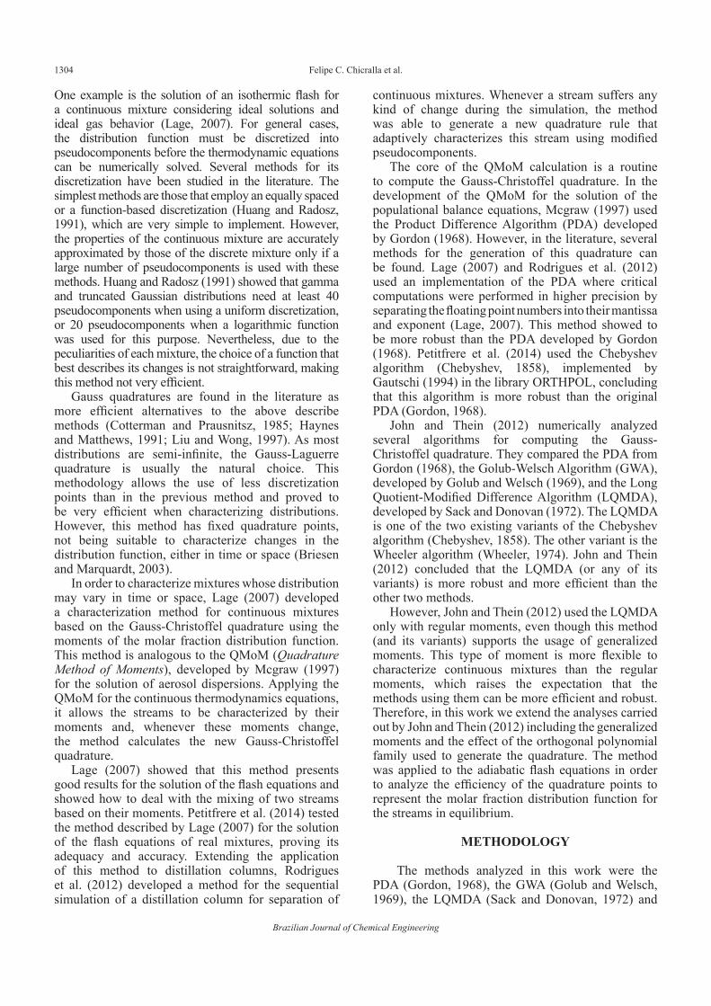
One example is the solution of an isothermic flash for a continuous mixture considering ideal solutions and ideal gas behavior (Lage, 2007). For general cases, the distribution function must be discretized into pseudocomponents before the thermodynamic equations can be numerically solved. Several methods for its discretization have been studied in the literature. The simplest methods are those that employ an equally spaced or a function-based discretization (Huang and Radosz, 1991), which are very simple to implement. However, the properties of the continuous mixture are accurately approximated by those of the discrete mixture only if a large number of pseudocomponents is used with these methods. Huang and Radosz (1991) showed that gamma and truncated Gaussian distributions need at least 40 pseudocomponents when using a uniform discretization, or 20 pseudocomponents when a logarithmic function was used for this purpose. Nevertheless, due to the peculiarities of each mixture, the choice of a function that best describes its changes is not straightforward, making this method not very efficient.

Gauss quadratures are found in the literature as more efficient alternatives to the above describe methods (Cotterman and Prausnitsz, 1985; Haynes and Matthews, 1991; Liu and Wong, 1997). As most distributions are semi-infinite, the Gauss-Laguerre quadrature is usually the natural choice. This methodology allows the use of less discretization points than in the previous method and proved to be very efficient when characterizing distributions. However, this method has fixed quadrature points, not being suitable to characterize changes in the distribution function, either in time or space (Briesen and Marquardt, 2003).

In order to characterize mixtures whose distribution may vary in time or space, Lage (2007) developed a characterization method for continuous mixtures based on the Gauss-Christoffel quadrature using the moments of the molar fraction distribution function. This method is analogous to the QMoM (Quadrature Method of Moments), developed by Mcgraw (1997) for the solution of aerosol dispersions. Applying the QMoM for the continuous thermodynamics equations, it allows the streams to be characterized by their moments and, whenever these moments change, the method calculates the new Gauss-Christoffel quadrature.

Lage (2007) showed that this method presents good results for the solution of the flash equations and showed how to deal with the mixing of two streams based on their moments. Petitfrere et al. (2014) tested the method described by Lage (2007) for the solution of the flash equations of real mixtures, proving its adequacy and accuracy. Extending the application of this method to distillation columns, Rodrigues et al. (2012) developed a method for the sequential simulation of a distillation column for separation of

continuous mixtures. Whenever a stream suffers any kind of change during the simulation, the method was able to generate a new quadrature rule that adaptively characterizes this stream using modified pseudocomponents.

The core of the QMoM calculation is a routine to compute the Gauss-Christoffel quadrature. In the development of the QMoM for the solution of the populational balance equations, Mcgraw (1997) used the Product Difference Algorithm (PDA) developed by Gordon (1968). However, in the literature, several methods for the generation of this quadrature can be found. Lage (2007) and Rodrigues et al. (2012) used an implementation of the PDA where critical computations were performed in higher precision by separating the floating point numbers into their mantissa and exponent (Lage, 2007). This method showed to be more robust than the PDA developed by Gordon (1968). Petitfrere et al. (2014) used the Chebyshev algorithm (Chebyshev, 1858), implemented by Gautschi (1994) in the library ORTHPOL, concluding that this algorithm is more robust than the original PDA (Gordon, 1968).

John and Thein (2012) numerically analyzed several algorithms for computing the Gauss-Christoffel quadrature. They compared the PDA from Gordon (1968), the Golub-Welsch Algorithm (GWA), developed by Golub and Welsch (1969), and the Long Quotient-Modified Difference Algorithm (LQMDA), developed by Sack and Donovan (1972). The LQMDA is one of the two existing variants of the Chebyshev algorithm (Chebyshev, 1858). The other variant is the Wheeler algorithm (Wheeler, 1974). John and Thein (2012) concluded that the LQMDA (or any of its variants) is more robust and more efficient than the other two methods.

However, John and Thein (2012) used the LQMDA only with regular moments, even though this method (and its variants) supports the usage of generalized moments. This type of moment is more flexible to characterize continuous mixtures than the regular moments, which raises the expectation that the methods using them can be more efficient and robust. Therefore, in this work we extend the analyses carried out by John and Thein (2012) including the generalized moments and the effect of the orthogonal polynomial family used to generate the quadrature. The method was applied to the adiabatic flash equations in order to analyze the efficiency of the quadrature points to represent the molar fraction distribution function for the streams in equilibrium.

METHODOLOGY

The methods analyzed in this work were the PDA (Gordon, 1968), the GWA (Golub and Welsch, 1969), the LQMDA (Sack and Donovan, 1972) and

Quadrature Algorithms for Phase Equilibrium of Continuous Mixtures

Brazilian Journal of Chemical Engineering, Vol. 36, No. 03, pp. 1303 - 1318, July - September, 2019

1305

the Chebyshev algorithm (Chebyshev, 1858), which can be found in Upadhyay (2012). All of them were applied using regular moments and the last two were also tested using generalized moments.

In order to analyze these methods that generate the Gauss-Christoffel quadrature, a computational program was implemented that, given a molar fraction distribution function, calculates the moments of this distribution, generates its quadrature rule and, when required, solves the adiabatic flash equations for the composition of the pseudocomponents of the equilibrium streams. The procedures and equations used in this program are detailed in this section. The development of these methods can be found in the original references and also in John and Thein (2012). Therefore, their details are not given here.

Moments calculationConsider a molar fraction distribution, f(x), in

terms of a characterization variable, x, defined in the interval [a, b]. This distribution can be characterized by its regular moments, defined as:

Computation of the quadratureThe studied algorithms generate the quadrature [xj,

ωj]nj=1, that optimally approximates the integral:

( ) , 0,1, 2,...µ = =∫b

kk

a

x f x dx k

where k is the order of the moment. These moments carry information of the distribution that is used by the algorithms to generate the desired Gauss-Christoffel quadrature.

There are also the generalized moments of the distribution that are obtained by substituting the monomial xk in Equation (1) by the k-order polynomial, pk(x), of an orthogonal polynomial family, resulting in:

( ) ( ) ( ) , 0,1, 2,...µ = =∫b

Pk k

a

p x f x dx k

where µk(P) is the generalized moment of order k

associated with this orthogonal polynomial family, which can be obtained by the following recursion formula:

( )( )( ) ( ) ( ) ( )

1

0

1 1

01

, 0,1,...

−

+ −

=== + + =k k k k k k k

p xp xxp x a p x b p x c p x k

where the coefficients ak, bk and ck define the given family. It is important to note that the generalized moments are reduced to the regular moments for ak = 1 and bk = ck = 0.

Once calculated the n quadrature points, the first 2n regular or generalized moments from the distribution can be reconstructed respectively from:

( )1

, 0,..., 2 1=

µ = = −∑n

kk i i

i

x f x k n

( ) ( ) ( )1

, 0,..., 2 1=

µ = = −∑n

Pk k i i

i

p x f x k n

( ) ( ) ( )1=

≈ ω∑∫b n

j jja

g x f x dx g x

where f(x) is the molar fraction distribution function and g(x) is a given property of the mixture component x with infinitesimal molar fraction f(x)dx. By interpreting Equation (6) as a discretization of the mixture, the abscissas, xj, represent pseudocomponents and the weights, ωj, are their molar fraction.

The inner product between two functions p(x) and q(x) with respect to the weight function f(x) in the interval [a, b] is defined as:

( ) ( ) ( ),⟨ ⟩ ≡ ∫b

a

p q p x q x f x dx

As for any Gaussian quadrature rule, the abscissa of the quadrature given by Equation (6) are the roots of the n-order polynomial of the Christoffel orthogonal polynomial family using the inner product defined by Equation (7). However, since f(x) is the unknown mixture molar fraction distribution, it is impossible to have a priori knowledge of the recursion coefficients of the corresponding orthogonal polynomial family. Therefore, the quadrature rule must be numerically computed from the known moments of the distribution function, as detailed in the following.

These Christoffel orthogonal polynomials are generated by the following recursion:

( )( )( ) ( ) ( ) ( )

1

02

1 1

01

, 0,1,...

−

+ −

=== −θ −η =k k k k k

P xP xP x x P x P x k

where Pk(x) is the Christoffel polynomial of order k and the coefficients k and θk can be obtained by:

, , 0,

⟨ ⟩θ = ≥

⟨ ⟩k k

kk k

xP P kP P

(1)

(2)

(3)

(4)

(5)

(6)

(7)

(8)

(9)



1306

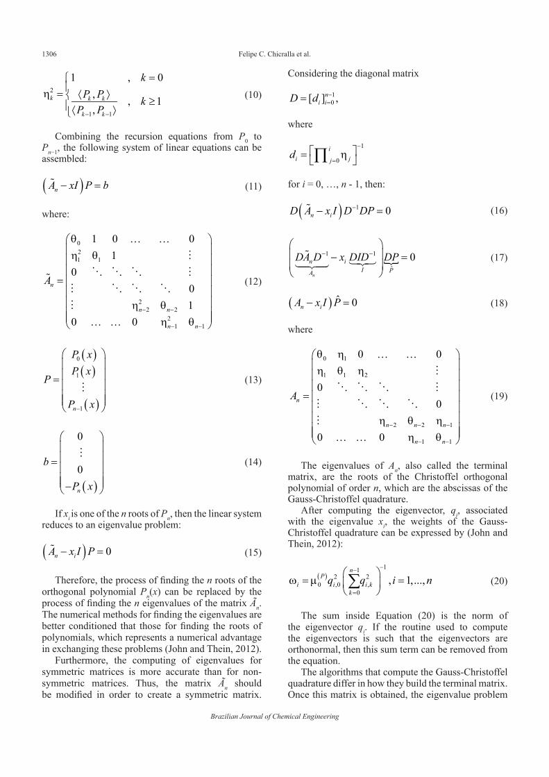
Combining the recursion equations from P0 to Pn−1, the following system of linear equations can be assembled:

Considering the diagonal matrix2

1 1

1 , 0, , 1,− −

=η = ⟨ ⟩ ≥⟨ ⟩

k k k

k k

kP P k

P P(10)

( )− =

nA xI P b

where:

021 1

22 2

21 1

1 0 01

001

0 0− −

− −

θ … … η θ

= η θ … … η θ

n

n n

n n

A

( )( )

( )

0

1

1

−

=

n

P xP x

P

P x

( )

0 0

= −

n

b

P x

If xi is one of the n roots of Pn, then the linear system reduces to an eigenvalue problem:

( ) 0− =

n iA x I P

Therefore, the process of finding the n roots of the orthogonal polynomial Pn(x) can be replaced by the process of finding the n eigenvalues of the matrix Ãn. The numerical methods for finding the eigenvalues are better conditioned that those for finding the roots of polynomials, which represents a numerical advantage in exchanging these problems (John and Thein, 2012).

Furthermore, the computing of eigenvalues for symmetric matrices is more accurate than for non-symmetric matrices. Thus, the matrix Ãn should be modified in order to create a symmetric matrix.

10] ,[ −

== ni iD d

where

1

0

−

= = η ∏ i

i jjd

for i = 0, …, n - 1, then:

( ) 1 0−− =

n iD A x I D DP

1

ˆ

1 0− − − =

n

n iI PA

DA D x DID DP

( ) 0ˆ− =n iA x I P

where

0 1

1 1 2

2 2 1

1 1

0 0

00

0 0− − −

− −

θ η … … η θ η

= η θ η … … η θ

n

n n n

n n

A

The eigenvalues of An, also called the terminal matrix, are the roots of the Christoffel orthogonal polynomial of order n, which are the abscissas of the Gauss-Christoffel quadrature.

After computing the eigenvector, qi, associated with the eigenvalue xi, the weights of the Gauss-Christoffel quadrature can be expressed by (John and Thein, 2012):

( )11

2 20 ,0 ,

0

, 1,...,−−

=

ω = µ =

∑n

Pi i i k

k

q q i n

The sum inside Equation (20) is the norm of the eigenvector qi. If the routine used to compute the eigenvectors is such that the eigenvectors are orthonormal, then this sum term can be removed from the equation.

The algorithms that compute the Gauss-Christoffel quadrature differ in how they build the terminal matrix. Once this matrix is obtained, the eigenvalue problem

(11)

(12)

(13)

(14)

(15)

(16)

(17)

(18)

(19)

(20)



1307

is solved in the same way for all methods. All methods use the moments of the distribution as the necessary information to build the matrix An. For a quadrature with n points, the first 2n moments must be known.

Considering the analyzed methods, it is important to highlight that only the LQMDA and the Chebyshev Algorithm can use both regular and generalized moments as input. Also, the PDA was tested in two different implementations: the original version by Gordon (1968) and the modified implementation given by Lage (2007).

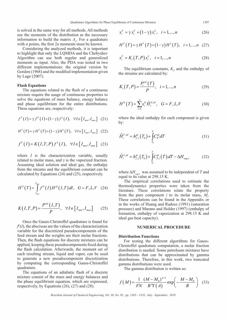
Flash EquationsThe equations related to the flash of a continuous

mixture require the usage of continuous properties to solve the equations of mass balance, energy balance and phase equilibrium for the entire distributions. These equations are, respectively:

where the ideal enthalpy for each component is given by:

( ) ( ) ( ) ( ) [ ]1 , ,= γ + − γ ∀ ∈F V Lmin maxf I f I f I I I I

( ) ( ) ( ) ( ) [ ]1 , ,= γ + − γ ∀ ∈F V Lmin maxH T H T H T I I I

( ) ( ) ( ) [ ], , , ,= ∀ ∈V Lmin maxf I K I T P f I I I I

where I is the characterization variable, usually related to molar mass, and γ is the vaporized fraction. Assuming ideal solution and ideal gas, the enthalpy from the streams and the equilibrium constant can be calculated by Equations (24) and (25), respectively.

( ) ( ) ( ), , , ,= =∫max

min

IG G gi

I

H T f I H I T dI G F L V

( ) ( ) [ ],, , , ,= ∀ ∈

sat

min max

P I TK I T P I I I

P

Once the Gauss-Christoffel quadrature is found for fF(I), the abscissas are the values of the characterization variable for the discretized pseudocomponents of the feed stream and the weights are their molar fractions. Then, the flash equations for discrete mixtures can be applied, keeping these pseudocomponents fixed during the flash calculation. Afterwards, the moment set of each resulting stream, liquid and vapor, can be used to generate a new pseudocomponent discretization by computing the corresponding Gauss-Christoffel quadrature.

The equations of an adiabatic flash of a discrete mixture consist of the mass and energy balances and the phase equilibrium equation, which are expressed, respectively, by Equations (26), (27) and (28).

( )1 , 1,...,= γ + − γ =F V Li i ix x x i n

( ) ( ) ( ) ( )1 , 1,...,= γ + − γ =F V LH T H T H T i n

( ), , 1,...,= =V Li i ix K T P x i n

The equilibrium constants, Ki, and the enthalpy of the streams are calculated by:

( ) ( ), , 1,...,= =sat

ii

P TK T P i n

P

( ) ,

1

ˆ , , ,=

= =∑n

G G G idi i

i

H T x H G F L V

( )0

,, 0

ˆ = + ∫T

V id gi gii f i P

T

H h T C dT

( ) ( )0

,, 0 , ,

ˆ = + −∆∫T

L id gi gii f i P i vap i

T

H h T C T dT H

where ΔHvap,i was assumed to be independent of T and equal to its value at 298.15 K.

The empirical correlations used to estimate the thermodynamics properties were taken from the literature. These correlations relate the property from the pure component i to its molar mass, Mi. These correlations can be found in the Appendix or in the works of Huang and Radosz (1991) (saturation pressure) and Marano and Holder (1997) (enthalpy of formation, enthalpy of vaporization at 298.15 K and ideal gas heat capacity).

NUMERICAL PROCEDURE

Distribution FunctionsFor testing the different algorithms for Gauss-

Christoffel quadrature computation, a molar fraction distribution is needed. Some petroleum mixtures have distributions that can be approximated by gamma distributions. Therefore, in this work, two truncated gamma distributions were used.

The gamma distribution is written as:

( ) ( )1

0 0( )1 exp−− − = − Γ

A

A

M M M MfN BF

MB A

(21)

(22)

(23)

(24)

(25)

(26)

(27)

(28)

(29)

(30)

(31)

(32)

(33)



1308

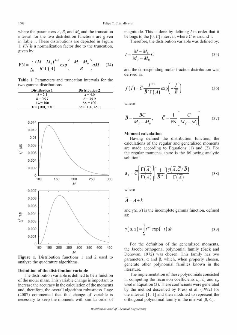
where the parameters A, B, and M0 and the truncation interval for the two distribution functions are given in Table 1. These distributions are depicted in Figure 1. FN is a normalization factor due to the truncation, given by:

magnitude. This is done by defining I in order that it belongs to the [0, C] interval, where C is around 1.

Therefore, the distribution variable was defined by:

( )1

0 0( )FN exp−

∆

− − = − Γ ∫A

AM

M M M M dMB A B

Table 1. Parameters and truncation intervals for the two gamma distributions.

Figure 1. Distribution functions 1 and 2 used to analyze the quadrature algorithms.

Definition of the distribution variableThe distribution variable is defined to be a function

of the molar mass. This variable change is important to increase the accuracy in the calculation of the moments and, therefore, the overall algorithm robustness. Lage (2007) commented that this change of variable is necessary to keep the moments with similar order of

0

0

−=

−f

M MI CM M

and the corresponding molar fraction distribution was derived as:

( ) ( )1

exp− = − Γ

A

A

I If I CB A B

where

0 0

1, FN

= =

− − f f

BC CB CM M M M

Moment calculationHaving defined the distribution function, the

calculations of the regular and generalized moments are made according to Equations (1) and (2). For the regular moments, there is the following analytic solution:

( )( )

( )( ), /1

−

Γ γ µ = Γ Γ k k

A A C BC

A B A

where

= +A A k

and γ(a, x) is the incomplete gamma function, defined as:

( ) ( )1

0

, exp−γ = −∫x

aa x t t dt

For the definition of the generalized moments, the Jacobi orthogonal polynomial family (Sack and Donovan, 1972) was chosen. This family has two parameters, α and β, which, when properly chosen, generate other polynomial families known in the literature.

The implementation of these polynomials consisted in computing the recursion coefficients ak, bk and ck, used in Equation (3). These coefficients were generated by the method described by Press et al. (1992) for the interval [1, 1] and then modified to represent the orthogonal polynomial family in the interval [0, C].

(34)

(35)

(36)

(37)

(38)

(39)



1309

Adiabatic flash calculationOnce the distribution function was discretized,

the resulting composition was used for the adiabatic flash calculations, whose methodology can be found in Henley et al. (2011).

The methodology results in finding the composition of both vapor (xi

V) and liquid (xiL) phases, the flash

temperature (Tflash) as well as the vaporized fraction (γ) of the flash, with the feed stream and flash conditions given in Table 2.

Test 2: Choice of distribution variable. The value of the parameter C was varied from 0.5 to 2.0 and its influence on the values of the 20 first reconstructed moments was analyzed for methods using either regular or generalized moments. Besides, for each value of C, the maximum number of quadrature points that can be computed by the method (nmax) and the associated MSRE were evaluated as a measure of the method robustness.

Test 3: Choice of orthogonal polynomial family. Aiming at analysing the influence of the choice of the orthogonal polynomial family used to compute the generalized moments, the values of the parameters of the Jacobi polynomial were varied from -0.5 to 2.0. Some of the chosen parameter values generate polynomial families known in the literature, as shown in Table 4. The values of the 20 first reconstructed moments were compared and the maximum number of quadrature points achieved by the method (nmax) and the associated MSRE were also evaluated.

Test 4: Adiabatic flash solution. For this test, only the LQMDA using generalized moments was employed with C = 1 using the Jacobi polynomials with α = β = 2. The adiabatic flash was computed using different values for the number of quadrature points and the accuracy of the following properties of the streams were analyzed.

• Bubble point temperature of the feed stream at flash pressure (Tbub);

• Dew point temperature of the feed stream at flash pressure (Tdew);

• Flash temperature at flash pressure (Tflash); • Vapor fraction for the adiabatic flash (γflash); • Mean molar mass for the feed, vapor and liquid

streams (MF, MV, ML). The mean molar mass of a stream G is given by:

Table 2. Adiabatic flash conditions.

Conditions for the numerical analysisTable 3 lists the methods compared for generating

the quadrature and the type of moments employed by them. The analysis of the efficiency and robustness of these algorithms was carried out by calculating the computational cost and the errors in the reconstructed moments.

The computational cost was measured by the function clock, inside the file time.h (in C language). This function was called before and after each routine that computes the quadrature and, therefore, the reported CPU clocks are just for the quadrature computation.

The error of the reconstructed moments was calculated as the mean square of the relative errors (MSRE) of the moments between the analytical moments, given by Equations (1) or (2) (µk,dist), and the reconstructed moments, given by Equations (4) or (5) (µk,reconst), according to:

Table 3. Methods analyzed.

22 1

, ,

0 ,

12

−

=

µ −µ= µ

∑n

k dist k reconst

k k dist

MSREn

Test 1: Efficiency of the methods. The parameter C was kept equal to 1 and the computational cost and the MSRE were computed for all cases, varying the number of quadrature points from 3 to 20. Ten runs of the computer program were used to evaluate the computational cost, giving its mean value and standard deviation.

Table 4. Parameters of the Jacobi polynomial families.

, , ,= =∑G G Gi iM M x G F L V

These properties were compared to those obtained by using a uniform discretization of the feed molar fraction distribution using 10 to 10,000 pseudocomponents.

The moments for the liquid and vapor streams were computed from the flash results. Then, for each stream, a new characterization was calculated by computing a new Gauss-Christoffel quadrature. This was used to

(40)

(41)



1310

obtain the reconstructed moments of the stream and the corresponding MSRE values.

RESULTS

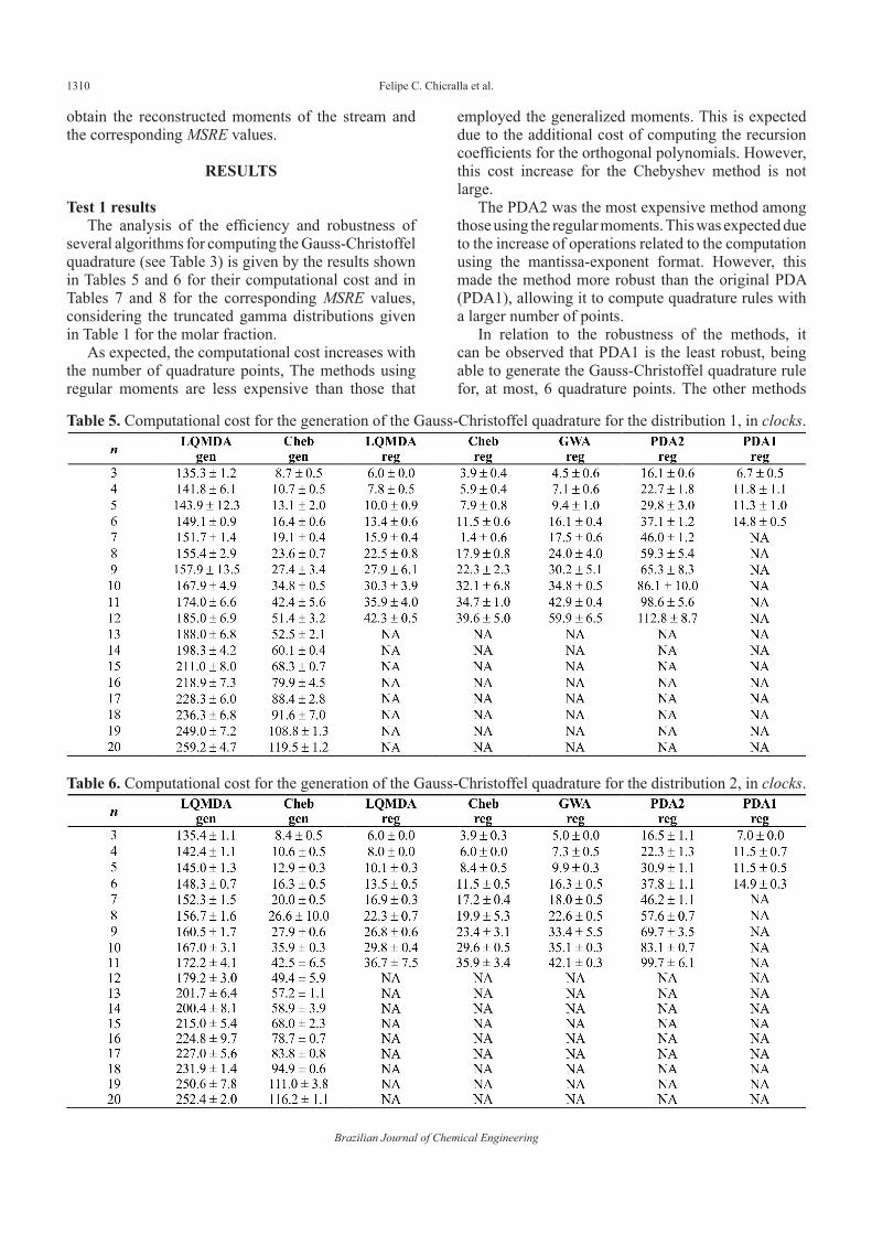
Test 1 resultsThe analysis of the efficiency and robustness of

several algorithms for computing the Gauss-Christoffel quadrature (see Table 3) is given by the results shown in Tables 5 and 6 for their computational cost and in Tables 7 and 8 for the corresponding MSRE values, considering the truncated gamma distributions given in Table 1 for the molar fraction.

As expected, the computational cost increases with the number of quadrature points, The methods using regular moments are less expensive than those that

employed the generalized moments. This is expected due to the additional cost of computing the recursion coefficients for the orthogonal polynomials. However, this cost increase for the Chebyshev method is not large.

The PDA2 was the most expensive method among those using the regular moments. This was expected due to the increase of operations related to the computation using the mantissa-exponent format. However, this made the method more robust than the original PDA (PDA1), allowing it to compute quadrature rules with a larger number of points.

In relation to the robustness of the methods, it can be observed that PDA1 is the least robust, being able to generate the Gauss-Christoffel quadrature rule for, at most, 6 quadrature points. The other methods

Table 5. Computational cost for the generation of the Gauss-Christoffel quadrature for the distribution 1, in clocks.

Table 6. Computational cost for the generation of the Gauss-Christoffel quadrature for the distribution 2, in clocks.



1311

using regular moments have similar behaviors among themselves, being able to compute the quadrature rule up to 12 points for distribution 1 and 11 points for distribution 2.

When analyzing the MSRE, although there are some oscillations, it can be noted that the MSRE tends to increase with the number of quadrature points due to error accumulation. The only exception was the GWA, for which the MSRE decreased by orders of magnitude as n increases. The reason for this behavior is that this method requires the usage of an additional moment of order 2n, which is the main factor responsible for the MSRE values for this method, because the n−point quadrature can only exactly compute the first 2n moments. For this method, the increase of the number of quadrature points increased the accuracy of this extra moment.

The methods using generalized moments were able to obtain the Gauss-Christoffel quadrature rule for more than 20 points for both distributions, showing that these methods are more robust than those using regular moments. The MSRE for these methods were slightly higher than for the other methods. However, these errors are of the order of 10−13, which is still very small for generating the Gauss-Christoffel quadrature rule for a large number of quadrature points.

Similarly to the results of John and Thein (2012), the LQMDA and the Chebyshev method were found to be equivalent in robusteness and computational cost when both used the regular moment set. However, for the generalized moment set, the Chebyshev method is much faster. For instance, considering the largest n value (11) for which the LQMDA and the Chebyshev

Table 7. MSRE in the reconstructed moments for the distribution 1.

Table 8. MSRE in the reconstructed moments for the distribution 2.



1312

method were able to compute the quadrature using both the generalized and regular moment sets for both distributions, the increase in the computational cost related to the usage of the generalized moments is about 376% for LQMDA and only 20% for the Chebyshev method.

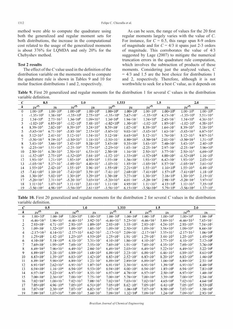
Test 2 resultsThe effect of the C value used in the definition of the

distribution variable on the moments used to compute the quadrature rule is shown in Tables 9 and 10 for molar fraction distributions 1 and 2, respectively.

As can be seen, the range of values for the 20 first regular moments largely varies with the value of C. For instance, for C = 0.5, this range span 8-9 orders of magnitude and for C = 4/3 it spans just 2-3 orders of magnitude. This corroborates the value of 4/3 suggested by Lage (2007) to mitigate the numerical truncation errors in the quadrature rule computation, which involves the subtraction of products of these moments. Considering just the analyzed values, C = 4/3 and 1.5 are the best choice for distributions 1 and 2, respectively. Therefore, although it is not worthwhile to seek for a best C value, as it depends on

Table 9. First 20 generalized and regular moments for the distribution 1 for several C values in the distribution variable definition.

Table 10. First 20 generalized and regular moments for the distribution 2 for several C values in the distribution variable definition.



1313

the distribution, a choice of C within [4/3, 3/2] seems to be a good rule of thumb.

On the other hand, the value of C had no effect in the range of values of the generalized moments. This was expected because the change of variable made in the distribution function was also carried out in the orthogonal polynomials to maintain their orthogonality in the desired interval.

The effect of the distribution variable definition on the robustness and the efficiency of the methods can be analyzed from the maximum number of quadrature points for which the methods were able to generate the quadrature rule and the corresponding MSRE values, which are shown in Tables 11 and 12 for molar fraction distributions 1 and 2, respectively.

As the order of magnitude of the generalized moments were not affected by the value of C used in the definition of the distribution variable, the maximum number of quadrature points does not change with it for the methods using such moments. Moreover, the corresponding MSRE values are basically independent of the C value.

On the other hand, the methods using the regular moments were affected by the value of C, notably

PDA1, whose nmax value increased with the C value. This was not expected because the magnitude of the regular moments also increased with the the C value.

The other methods were able to calculate quadrature rules with 11-12 points without following any specific pattern. The MSRE values were around 10−14 - 10−15 for the PDA2, LQMDA-reg and Cheb-reg. The MSRE for GWA were higher, of the order of magnitude of 10−13 to 10−12, but this can be explained by the error accumulation caused by the additional moment of order 2nmax.

Test 3 resultsThe results regarding the choice of the orthogonal

polynomial family to generate the generalized moments were obtained by varying the values of the parameters α and β of the Jacobi polynomial family, The results for the distributions 1 and 2 are shown in Tables 13 and 14, respectively. It can be observed that the values of the 20 first generalized moments span a range that is reduced when the values of α and β were increased. For the tested values, it was observed that the generalized moments of the Legendre polynomials

Table 12. Maximum number of quadrature points obtained for the Gauss-Christoffel quadrature for the distribution 2 for several C values in the distribution variable definition and the corresponding MSRE values.

Table 11. Maximum number of quadrature points obtained for the Gauss-Christoffel quadrature for the distribution 1 for several C values in the distribution variable definition and the corresponding MSRE values.



1314

Table 13. Generalized moments for the distribution 1 for some orthogonal polynomial families.

Table 14. Generalized moments for the distribution 2 for some orthogonal polynomial families.

had the largest order of magnitude range, that is, |µ0(P)

/ µk(P)| ~ 105 and 106, k = 1, …, 20, for the distributions

1 and 2, respectively.The results for the nmax and the MSRE values are

shown in Tables 15 and 16 for the distributions 1 and 2, respectively. The computations using the Chebyshev polynomials of 1st order (α = β = −0.5) had the lowest value of nmax for distribution 2 and presented the highest order of magnitude for the MSRE for both distributions. The Legendre polynomials (α = β = 0) also showed large values for the MSRE for both distributions. The Jacobi polynomials with α = β = 1

or α = β = 2 showed low MSRE values, making them good choices for the cases analyzed.

Test 4 resultsFor the adiabatic flashes of both distributions,

according to the conditions given in Table 2, the results for the MSRE values and for some properties of the equilibrium streams for several numbers of discretization points are shown in Tables 17 and 18 for the distributions 1 and 2, respectively. It should be noted that the MSRE values for the liquid and vapor streams are those computed after the re-characterization of



1315

each stream, being similar to the MSRE results shown in Section 4.1 for the feed distributions.

It can be observed that the discretization using the Gauss-Christoffel quadrature was not only capable of representing well both mixture properties, but it also does this with a much smaller number of discretization points. For both distributions, 8 quadrature points were enough to accurately represent the properties of these mixtures. For uniform discretizations of these mixtures, Tables 17 and 18 show that the number of pseudocomponents has to be around 104 in order to achieve similar accuracy in the computation of the mixture properties.

Above 8 quadrature points, the Gauss-Christoffel quadrature discretization obtained the same values for all the properties of the streams, showing the good convergence of this method. The usage of more than 8 quadrature points only increased the MSRE values as already discussed.

For the uniform discretization method, it can be seen that its convergence is very slow, which can be verified by the fact that the stream properties still vary for n > 1000. Due to the large number of pseudocomponents that is needed, their molar fraction became quite low. This leads to a large accumulation of truncation errors that precluded the computations for n > 10000 for both distributions.

Table 15. Maximum number of quadrature points obtained for the Gauss-Christoffel quadrature for the distribution 1 for some orthogonal polynomial families and the corresponding MSRE values.

Table 16. Maximum number of quadrature points obtained for the Gauss-Christoffel quadrature for the distribution 2 for some orthogonal polynomial families and the corresponding MSRE values.

Table 17. Stream properties for the adiabatic flash for distribution 1.



1316

CONCLUSION

Among the methods compared for the computing of the Gauss-Christoffel quadrature, we concluded that those using generalized moments are more robust. Although these methods require a higher computational effort than those using regular moments, the gain in robustness is worthwhile as the number of quadrature points can be larger than 80. Even though this is an advantage, it might not be necessary as 8 pseudocomponents were shown to be enough for representing the properties of the streams involved in the adiabatic flash for the two mixtures analyzed in this work. The only disadvantage in using generalized moments is their larger computational cost. The usage of the generalized moment set made the LQMDA almost five times slower, whereas the Chebyshev algorithm showed just a 20% increase in its computational cost. Therefore, the Chebyshev algorithm using generalized moments is recommended to be used in the QMoM.

Due to the small number of pseudocomponents needed for accurate results, the QMoM proved to be an efficient and computationally cheap method for performing thermodynamic calculations for continuous and multicomponent mixtures, as also pointed out by Lage (2007), Rodrigues et al. (2012) and Petitfrere et al. (2014).

ACKNOWLEDGMENTS

Paulo L. C. Lage acknowledges the financial support from CNPq, grants #456905/2014-6 and 305265/2015-6. Argimiro R. Secchi acknowledges the financial support from CNPq, grant #302893/2013-0. This study was financed in part by the Coordenação de Aperfeiçoamento de Pessoal de Nível Superior - Brasil (CAPES) - Finance Code 001.

NOMENCLATURE

A Gamma distribution parameter An Terminal matrix ak Recursion coefficient for an orthogonal polynomial family of order k B Gamma distribution parameter bk Recursion coefficient for an orthogonal polynomial family of order kC Upper limit for the change of variable ck Recursion coefficient for an orthogonal polynomial family of order kCp Heat capacity D Diagonal matrix f Molar fraction distribution function FN Distribution normalization factor H Enthalpy ∆Hvap Enthalpy of vaporization Hf,i Enthalpy of formation

Table 18. Stream properties for the adiabatic flash for distribution 2.



1317

I Identity Matrix I Distribution variable K Equilibrium constant M Molar mass M Mean molar mass MSRE Mean square error N Number of quadrature points P Pressure Pk(x) Christoffel orthogonal polynomial of order kpk(x) Orthogonal polynomial of order kqi Eigenvector of the terminal matrix, associated with the eigenvalue xi T Temperature xi Abscissa of the Gauss-Christoffel quadrature

Greek letters α Parameter for the Jacobi polynomials β Parameter for the Jacobi polynomials ηk Recursion coefficient of the Christoffel orthogonal polynomial of order kγ Vaporized fraction Γ Gamma function µk Regular moment of order kµk

(P) Generalized moments of order kωi Weight from the Gauss-Christoffel quadratureθk Recursion coefficient of the Christoffel orthogonal polynomial of order k

Superscripts bub Bubble point dew Dew point F Feed stream flash Flash condition G Feed, vapor or liquid stream gi Ideal gas condition L Liquid stream sat Saturation condition V Vapor stream

REFERENCES

Briesen, H., Marquardt, W. An adaptative multigrid method for steady-state simulation of petroleum mixtures separation processes. Industrial & Engineering Chemical Research, 42, 2334-2348, 2003. https://doi.org/10.1021/ie0206150

Chebyshev, P. L. Sur les fractions continues. Journal de Mathématiques Pures et Appliquées, 3, 289-323, 1858.

Cotterman, R. L., Prausnitsz, J. M. Flash calculations for continuous or semicontinuous mixtures using an equation of state. Industrial and Engineering Chemistry Process Design and Development, 24, 434-443, 1985. https://doi.org/10.1021/i200029a038

Gautschi, W. Algorithm 726: ORTHPOL - a package of routines for generating orthogonal polynomials and

gauss-type quadrature rules. ACM Transactions on Mathematical Software, 20, 21-62, 1994. https://doi.org/10.1145/174603.174605

Golub, G. H., Welsch, J. H. Calculation of gauss quadrature rules. Mathematics of Computation, 23, 221-230, 1969. https://doi.org/10.2307/2004418

Gordon, R. Error bounds in equilibrium statistical mechanics. Journal of Mathematical Physics, 9, 655-663, 1968. https://doi.org/10.1063/1.1664624

Haynes, H. W., Matthews, M. A. Continuous-mixture vapor-liquid equilibria computations based on true boiling point distillations. Industrial & Engineering Chemical Research, 30, 1911-1915, 1991. https://doi.org/10.1021/ie00056a036

Henley, E. J., Seader, J. D., Roper, D. K. Separation process principles. Wiley, 2011. ISBN 9780470646113. https://Books.Google.Com.Br/Books?Id=Cuo8bwaacaaj.

Huang, S. H., Radosz, M. Phase behavior of reservouir fluids III: molecular lumping and characterization. Fluid Phase Equilibria, 66, 1-21, 1991. https://doi.org/10.1016/0378-3812(91)85044-U

John, V., Thein, F. On the efficiency and robustness of the core routine of the quadrature method of moments (QMOM). Chemical Engineering Science, 75, 327-333, 2012. https://doi.org/10.1016/j.ces.2012.03.024

Lage, P. L. C. The quadrature method of moments for continuous thermodynamics. Computers & Chemical Engineering, 31, 782-799, 2007. https://doi.org/10.1016/j.compchemeng.2006.08.005

Liu, J. L., Wong, D. S. H. Rigorous implementation of continuous thermodynamics using orthonormal polynomials. Fluid Phase Equilibra, 129, 113-127, 1997. https://doi.org/10.1016/S0378-3812(94)02678-5

Marano, J., Holder, G. A general equation for correlating the thermophysical properties of n-parafins, n-olefins, and other homologous series. 3. asymptotic behavior correlations for thermal and transport properties. Industrial Engineering Chemistry Research, 36, 2399-2408, 1997. https://doi.org/10.1021/ie9605138

Mcgraw, R. Description of aerosol dynamics by the quadrature method of moments. Aerosol Science and Technology, 27, 255-265, 1997. https://doi.org/10.1080/02786829708965471

Petitfrere, M., Nichita, D. V., Montel, F. Multiphase equilibrium calculations using the semicontinuous thermodynamics of hydrocarbon mistures. Fluid Phase Equilibria, 362, 365-378, 2014. https://doi.org/10.1016/j.fluid.2013.10.056

Press, W. H., Flannery, B. P., Teukolsky, S. A., Vetterling, W. T. Numerical recipes in C: The art of scientific computing. Cambridge University Press, 2 edition, 1992.



1318

Rodrigues, R. C., Ahon, V. R. R., Lage, P. L. C. An adaptative characterization scheme for the simulaion of multistage separation of continuous mixtures using the quadrature method of moments. Fluid Phase Equilibria, 318, 1-12, 2012. https://doi.org/10.1016/j.fluid.2012.01.015

Sack, R. A., Donovan, A. F. An algorithm for gaussian quadrature given modified moments. Numerische Mathematik, 18, 465-478, 1972. https://doi.org/10.1007/BF01406683

Upadhyay, R. R. Evaluation of the use of the chebyshev algorithm with the quadrature method of moments for simulating aerosol dynamics. Journal of Aerosol Science, 44, 11-23, 2012. https://doi.org/10.1016/j.jaerosci.2011.09.005

Wheeler, J. C. Modified moments and gaussian quadratures. Journal of Mathematics, 4, 287-296, 1974. https://doi.org/10.1216/RMJ-1974-4-2-287

Whitson, C., Brule, M. (Editors). Phase Behavior. SPE, Texas, 2000.

APPENDIX

Properties CorrelationsIn this appendix, the correlations found in the

literature for the estimation of the properties of the generated pseudocomponents are listed.

Saturation Pressure (Huang and Radosz, 1991):

where [Psat] = Pa, and [T] = K.Ideal Gas Heat Capacity (Marano and Holder,

(1997):

1 9.5046 0.016104= +B M

( )( )2 exp 5.0237 0.72702= +B ln M

( )1 2100000exp /= −satP B B T

( ) ( ) ( )( )( )

6 2 9 30.0919055 0.011308 6.3792010 1.4060510

0.284370

− −= − + − +

+

giP

c

C T K T K T K

N R

where Nc = (M - 2)/14, R is the ideal gas constant and [CP

gi] = [R].Ideal Gas Enthalpy of Formation (Marano and

Holder, 1997):

( ) 08.3206 2.111890= − +gif ch N RT

where [hfgi] = [R][T0] and T0 = 298.15 K.

Enthalpy of Vaporization (Marano and Holder, 1997):

( )( ) 01 1.99516 0.112756∆ = + −VapcH N RT

where [ΔHVap] = [R][T0].

(42)

(43)

(44)

(45)

(46)

(47)

QUADRATURE ALGORITHMS FOR PHASE EQUILIBRIUM OF …

Documents

Transcript of QUADRATURE ALGORITHMS FOR PHASE EQUILIBRIUM OF …