1 Quadratic functions A. Quadratic functions B. Quadratic equations C. Quadratic inequalities.
Quadratic Formsand Their Applications
Proceedings of the Conference onQuadratic Forms and Their Applications
July 5–9, 1999University College Dublin
Eva Bayer-FluckigerDavid Lewis
Andrew RanickiEditors
Published as Contemporary Mathematics 272, A.M.S. (2000)

vii
Contents
Preface ix
Conference lectures x
Conference participants xii
Conference photo xiv
Galois cohomology of the classical groupsEva Bayer-Fluckiger 1
Symplectic latticesAnne-Marie Berge 9
Universal quadratic forms and the fifteen theoremJ.H. Conway 23
On the Conway-Schneeberger fifteen theoremManjul Bhargava 27
On trace forms and the Burnside ringMartin Epkenhans 39
Equivariant Brauer groupsA. Frohlich and C.T.C. Wall 57
Isotropy of quadratic forms and field invariantsDetlev W. Hoffmann 73
Quadratic forms with absolutely maximal splittingOleg Izhboldin and Alexander Vishik 103
2-regularity and reversibility of quadratic mappingsAlexey F. Izmailov 127
Quadratic forms in knot theoryC. Kearton 135
Biography of Ernst Witt (1911–1991)Ina Kersten 155

viii
Generic splitting towers and generic splitting preparationof quadratic formsManfred Knebusch and Ulf Rehmann 173
Local densities of hermitian formsMaurice Mischler 201
Notes towards a constructive proof of Hilbert’s theoremon ternary quarticsVictoria Powers and Bruce Reznick 209
On the history of the algebraic theory of quadratic formsWinfried Scharlau 229
Local fundamental classes derived from higher K-groups: IIIVictor P. Snaith 261
Hilbert’s theorem on positive ternary quarticsRichard G. Swan 287
Quadratic forms and normal surface singularitiesC.T.C. Wall 293

ix
Preface
These are the proceedings of the conference on “Quadratic Forms AndTheir Applications” which was held at University College Dublin from 5th to9th July, 1999. The meeting was attended by 82 participants from Europeand elsewhere. There were 13 one-hour lectures surveying various appli-cations of quadratic forms in algebra, number theory, algebraic geometry,topology and information theory. In addition, there were 22 half-hour lec-tures on more specialized topics.
The papers collected together in these proceedings are of various types.Some are expanded versions of the one-hour survey lectures delivered at theconference. Others are devoted to current research, and are based on thehalf-hour lectures. Yet others are concerned with the history of quadraticforms. All papers were refereed, and we are grateful to the referees for theirwork.
This volume includes one of the last papers of Oleg Izhboldin who diedunexpectedly on 17th April 2000 at the age of 37. His untimely death is agreat loss to mathematics and in particular to quadratic form theory. Weshall miss his brilliant and original ideas, his clarity of exposition, and hisfriendly and good-humoured presence.
The conference was supported by the European Community under theauspices of the TMR network FMRX CT-97-0107 “Algebraic K-Theory,Linear Algebraic Groups and Related Structures”. We are grateful to theMathematics Department of University College Dublin for hosting the con-ference, and in particular to Thomas Unger for all his work on the TEX andweb-related aspects of the conference.
Eva Bayer-Fluckiger, BesanconDavid Lewis, DublinAndrew Ranicki, Edinburgh
October, 2000

x
Conference lectures
60 minutes.
A.-M. Berge, Symplectic lattices.
J.J. Boutros, Quadratic forms in information theory.
J.H. Conway, The Fifteen Theorem.
D. Hoffmann, Zeros of quadratic forms.
C. Kearton, Quadratic forms in knot theory.
M. Kreck, Manifolds and quadratic forms.
R. Parimala, Algebras with involution.
A. Pfister, The history of the Milnor conjectures.
M. Rost, On characteristic numbers and norm varieties.
W. Scharlau, The history of the algebraic theory of quadratic forms.
J.-P. Serre, Abelian varieties and hermitian modules.
M. Taylor, Galois modules and hermitian Euler characteristics.
C.T.C. Wall, Quadratic forms in singularity theory.
30 minutes.
A. Arutyunov, Quadratic forms and abnormal extremal problems: someresults and unsolved problems.
P. Balmer, The Witt groups of triangulated categories, with some applica-tions.
G. Berhuy, Hermitian scaled trace forms of field extensions.
P. Calame, Integral forms without symmetry.
P. Chuard-Koulmann, Elements of given minimal polynomial in a centralsimple algebra.
M. Epkenhans, On trace forms and the Burnside ring.
L. Fainsilber, Quadratic forms and gas dynamics: sums of squares in adiscrete velocity model for the Boltzmann equation.
C. Frings, Second trace form and T2-standard normal bases.
J. Hurrelbrink, Quadratic forms of height 2 and differences of two Pfisterforms.
M. Iftime, On spacetime distributions.
A. Izmailov, 2-regularity and reversibility of quadratic mappings.
S. Joukhovitski, K-theory of the Weil transfer functor.

xi
V. Mauduit, Towards a Drinfeldian analogue of quadratic forms for poly-nomials.
M. Mischler, Local densities and Jordan decomposition.
V. Powers, Computational approaches to Hilbert’s theorem on ternaryquartics.
S. Pumplun, The Witt ring of a Brauer-Severi variety.
A. Queguiner, Discriminant and Clifford algebras of an algebra with in-volution.
U. Rehmann, A surprising fact about the generic splitting tower of a qua-dratic form.
C. Riehm, Orthogonal representations of finite groups.
D. Sheiham, Signatures of Seifert forms and cobordism of boundary links.
V. Snaith, Local fundamental classes constructed from higher dimensionalK-groups.
K. Zainoulline, On Grothendieck’s conjecture about principal homoge-neous spaces.

xii
Conference participants
A.V. Arutyunov, Moscow [email protected]. Balmer, Lausanne [email protected]. Bayer-Fluckiger, Besancon [email protected]. Becher, Besancon [email protected]. Berge, Talence [email protected]. Berhuy, Besancon [email protected]. Boutros, Paris [email protected]. Broecker, Muenster [email protected]. Calame, Lausanne [email protected]. Chuard-Koulmann, Louvain-la-Neuve [email protected]. Conway, Princeton [email protected]. Degos, Talence [email protected]. Dineen, Dublin [email protected]. Du Bois, Angers [email protected]. Elencwajg, Nice [email protected]. Elhamdadi, Trieste [email protected]. Elomary, Louvain-la-Neuve [email protected]. Epkenhans, Paderborn [email protected]. Fainsilber, Goteborg [email protected]. Flannery, Cork [email protected]. Frings, Besancon [email protected]. Garibaldi, Zurich [email protected]. Gille, Muenster [email protected]. Gindraux, Neuchatel [email protected]. Gow, Dublin [email protected]. Gradl, Duisburg [email protected]. Hellegouarch, Caen [email protected]. Hoffmann, Besancon [email protected]. Hurrelbrink, Baton Rouge [email protected]. Hutchinson, Dublin [email protected]. Iftime, Suceava [email protected]. Izmailov, Moscow [email protected]. Joukhovitski, Bonn [email protected]. Karoubi, Paris [email protected]. Kearton, Durham [email protected]. Kreck, Heidelberg [email protected]. Laffey, Dublin [email protected]. Lamy, Paris [email protected]. Leibak, Tallinn [email protected]. Lewis, Dublin [email protected]. Loday, Strasbourg [email protected]. Mackey, Dublin [email protected]
xiii
M. Marjoram, Dublin [email protected]. Mauduit, Dublin [email protected]. Mazzoleni, Lausanne [email protected]. McGarraghy, Dublin [email protected]. McGuire, Maynooth [email protected]. Mischler, Lausanne [email protected]. Monsurro, Besancon [email protected]. Morales, Baton Rouge [email protected]. Mulcahy, Atlanta [email protected]. Munkholm, Odense [email protected]. Parimala, Besancon [email protected]. Patashnick, Chicago [email protected]. Perret, Neuchatel [email protected]. Pfister, Mainz [email protected]. Powers, Atlanta [email protected]. Pumplun, Regensburg [email protected]. Queguiner, Paris [email protected]. Ranicki, Edinburgh [email protected]. Rehmann, Bielefeld [email protected]. Reich, Muenster [email protected]. Riehm, Hamilton, Ontario [email protected]. Rost, Regensburg [email protected]. Ryan, Dublin [email protected]. Scharlau, Muenster [email protected]. Scheiderer, Duisburg [email protected]. Serre, Paris [email protected]. Sheiham, Edinburgh [email protected]. Sigrist, Neuchatel [email protected]. Snaith, Southampton [email protected]. Taylor, Manchester [email protected]. Tignol, Louvain-la-Neuve [email protected]. Tipp, Ghent [email protected]. Tipple, Dublin [email protected]. Tuite, Galway [email protected]. Unger, Dublin [email protected]. Wall, Liverpool [email protected]. Yagunov, London Ontario [email protected]. Zahidi, Ghent [email protected]. Zainoulline, St. Petersburg [email protected]

xiv
Conference photo

xv
1
3
2
4
57
8
10
11
13
12
14
15
16
17
18
19
6
20
9
28
29
30
44
45
57
43
55
56
58
22
23
21
32
31
33
34
35
59
46
61
60
62
47
48
63
64
36
24
37
49
65
50
66 38
39
25
26
40
52
51
67
68
53
54
41
27
42
(1)
A.
Ranic
ki,
(2)
J.H
.C
onw
ay,
(3)
G.
Ele
ncw
ajg
,(4
)K
.Zain
oullin
e,
(5)
M.
Elo
mary
,(6
)V
.Snait
h,
(7)
S.
Pum
plu
n,
(8)
G.
Berh
uy,
(9)
A.Q
uequin
er,
(10)
M.D
uB
ois
,(1
1)
M.M
onsu
rro,(1
2)
V.M
auduit
,(1
3)
E.B
ayer-
Flu
ckig
er,
(14)
D.Lew
is,(1
5)
R.Pari
mala
,(1
6)
V.Pow
-ers
,(1
7)
F.
Sig
rist
,(1
8)
H.
Reic
h,
(19)
K.
Zahid
i,(2
0)
C.T
.C.
Wall,
(21)
H.
Munkholm
,(2
2)
M.
Ifti
me,
(23)
A.
Leib
ak,
(24)
C.
Fri
ngs,
(25)
C.
Rie
hm
,(2
6)
M.
Mis
chle
r,(2
7)
J.-P.
Serr
e,
(28)
S.
Perr
et,
(29)
A.-M
.B
erg
e,
(30)
W.
Sch
arl
au,
(31)
M.
Kre
ck,
(32)
S.
Gille
,(3
3)
J.-
Y.D
egos,
(34)
R.S
.G
ari
bald
i,(3
5)
S.M
cG
arr
aghy,
(36)
O.Pata
shnic
k,
(37)
Ph.D
uB
ois
,(3
8)
G.M
cG
uir
e,
(39)
C.M
ulc
ahy,
(40)
D.Sheih
am
,(4
1)
Ph.
Cala
me,
(42)
L.
Fain
silb
er,
(43)
J.-P.
Tig
nol,
(44)
J.-L.
Loday,
(45)
M.
Taylo
r,(4
6)
J.
Mora
les,
(47)
A.
Mazzole
ni,
(48)
C.
Sch
eid
ere
r,(4
9)A
.F.Iz
mailov,(5
0)K
.H
utc
hin
son,(5
1)A
.V.A
ruty
unov,(5
2)J.H
urr
elb
rink,(5
3)A
.Pfist
er,
(54)M
.R
ost
,(5
5)Y
.H
ellegouarc
h,(5
6)T
.U
nger,
(57)
P.C
huard
-Koulm
ann,(5
8)
D.H
offm
ann,(5
9)
M.G
indra
ux,(6
0)
U.T
ipp,(6
1)
M.Epkenhans,
(62)
T.J
.Laffey,(6
3)
K.J
.B
ech
er,
(64)
M.El-
ham
dadi,
(65)
F.G
radl,
(66)
P.B
alm
er,
(67)
D.Fla
nnery
,(6
8)
M.Tuit
e.
Contemporary MathematicsVolume 00, 2000
GALOIS COHOMOLOGY OFTHE CLASSICAL GROUPS
Eva Bayer–Fluckiger
Introduction
Galois cohomology sets of linear algebraic groups were first studied in the late50’s – early 60’s. As pointed out in [18], for classical groups, these sets have classicalinterpretations. In particular, Springer’s theorem [22] can be reformulated as aninjectivity statement for Galois cohomology sets of orthogonal groups; well–knownclassification results for quadratic forms over certain fields (such as finite fields,p–adic fields, . . . ) correspond to vanishing of such sets. The language of Galoiscohomology makes it possible to formulate analogous statements for other linearalgebraic groups. In [18] and [20], Serre raises questions and conjectures in thisspirit. The aim of this paper is to survey the results obtained in the case of theclassical groups.
1. Definitions and notation
Let k be a field of characteristic 6= 2, let ks be a separable closure of k and letΓk = Gal(ks/k).
1.1. Algebras with involution and norm–one–groups (cf. [9], [15]). LetA be a finite dimensional k–algebra. An involution σ : A → A is a k–linear antiau-tomorphism of A such that σ2 = id.
Let (A, σ) be an algebra with involution. The associated norm–one–group UA
is the linear algebraic group over k defined by
UA(E) = a ∈ A⊗ E |aσ(a) = 1
for every commutative k–algebra E.
1.2. Galois cohomology (cf. [20]). For any linear algebraic group U definedover k, set H1(k, U) = H1(Γk, U(ks)). Recall that H1(k, U) is also the set ofisomorphism classes of U–torsors (principal homogeneous spaces over U).
1.3. Cohomological dimension. Let k be a perfect field. We say that thecohomological dimension of k is ≤ n, denoted by cd(k) ≤ n, if Hi(Γk, C) = 0 forevery i > n and for every finite Γk–module C.
c©2000 American Mathematical Society
1

2 EVA BAYER–FLUCKIGER
We say that the virtual cohomological dimension of k is ≤ n, denoted byvcd(k) ≤ n, if there exists a finite extension k′ of k such that cd(k′) ≤ n. It isknown that this holds if and only if cd(k(
√−1)) ≤ n, see for instance [4], 1.2.
1.4. Galois cohomology mod 2. Set Hi(k) = Hi(Γk,Z/2Z). Recall thatwe have H1(k) ' k∗/k∗2 and H2(k) ' Br2(k).
If q '< a1, . . . , an > is a non–degenerate quadratic form, we define the discrim-inant of q by disc(q) = (−1)
n(n−1)2 a1 . . . an ∈ k∗/k∗2, and the Hasse–Witt invariant
by w2(q) = Σi<j(ai, aj) ∈ Br2(k).
1.5. Galois cohomology and quadratic forms. Let q be a non–degeneratequadratic form over k and let Oq be its orthogonal group. Then H1(k, Oq) is inbijection with the set of isomorphism classes of non–degenerate quadratic formsover k that become isomorphic to q over ks (equivalently, those which have thesame dimension as q) (cf. [20], III, 1.2. prop. 4).
2. Injectivity results
Some classical theorems of the theory of quadratic forms can be formulated interms of injectivity of maps between Galois cohomology sets H1(k, O), where O isan orthogonal group. This reformulation suggests generalisations to other linearalgebraic groups, as pointed out in [18] and [21]. The aim of this § is to give asurvey of the results obtained in this direction, especially in the case of the classicalgroups.
2.1. Springer’s theorem. Let q and q′ be two non–degenerate quadraticforms defined over k. Springer’s theorem [22] states that if q and q′ become iso-morphic over an odd degree extension, then they are already isomorphic over k.This can be reformulated in terms of Galois cohomology as follows. Let Oq be theorthogonal group of q. If L is an odd degree extension of k, then the canonical map
H1(k, Oq) → H1(L, Oq)
is injective.Serre makes this observation in [18], 5.3., and asks for generalisations of this
result to other linear algebraic groups. One has the following
Theorem 2.1.1. Let U be the norm–one–group of a finite dimensional k–algebra with involution. If L is an odd degree extension of k, then the canonicalmap
H1(k, U) → H1(L, U)is injective.
Proof. See [1], Theorem 2.1.
The above results concern injectivity after a base change. As noted in [21],some well–known results about quadratic forms can be reformulated as injectivitystatements of maps between Galois cohomology sets H1(k, U) → H1(k, U ′), whereU is a subgroup of U ′. This is for instance the case of Pfister’s theorem :
2.2. Pfister’s theorem. Let q, q′ and φ be non–degenerate quadratic formsover k. Suppose that the dimension of φ is odd. A classical result of Pfister saysthat if q ⊗ φ ' q′ ⊗ φ, then q ' q′ (see [15], 2.6.5.). This can be reformulated as

GALOIS COHOMOLOGY OF THE CLASSICAL GROUPS 3
follows. Denote by Oq the orthogonal group of q, and by Oq⊗φ the orthogonal groupof the tensor product q ⊗ φ. Then the canonical map H1(k, Oq) → H1(k, Oq⊗φ) isinjective. One can extend this result to algebras with involution as follows :
Theorem 2.2.1. Let (A, σ) and (B, τ) be finite dimensional k–algebras withinvolution. Let us denote by UA the norm–one–group of (A, σ), and by UA⊗B thenorm–one–group of the tensor product of algebras with involution (A, σ) ⊗ (B, τ).Suppose that dimk(B) is odd. Then the canonical map
H1(k, UA) → H1(k, UA⊗B)
is injective.
Note that Theorem 2.2.1 implies Pfister’s theorem quoted above, and also aresult of Lewis [10], Theorem 1.
For the proof of 2.2.1, we need the following consequence of Theorem 2.1.1.
Corollary 2.2.2. Let U and U ′ be norm–one–groups of finite dimensionalk–algebras. Suppose that there exists an odd degree extension L of k such thatH1(L,U) → H1(L,U ′) is injective. Then H1(k, U) → H1(k, U ′) is also injective.
Proof of 2.2.1. By a “devissage” as in [1], we reduce to the case where Aand B are central simple algebras with involution, that is either central over k withan involution of the first kind, or central over a quadratic extension k′ of k with ak′/k-involution of the second kind. Using 2.2.2, we may assume that B is split andthat the involution is given by a symmetric or hermitian form. We conclude theproof by the argument of [2], proof of Theorem 4.2.
It is easy to see that Theorem 2.2.1 does not extend to the case where bothalgebras have even degree.
2.3. Witt’s theorem. In 1937, Witt proved the “cancellation theorem” forquadratic forms [26] : if q1, q2 and q are quadratic forms such that q1 ⊕ q ' q2 ⊕ q,then q1 ' q2. The analog of this result for hermitian forms over skew fields alsoholds, see for instance [8] or [15].
These results can also be deduced from a statement on linear algebraic groupsdue to Borel and Tits :
Theorem 2.3.1. ([20], III.2.1., Exercice 1) Let G be a connected reductivegroup, and P a parabolic subgroup of G. Then the map H1(k, P ) → H1(k, G) isinjective.
3. Classification of quadratic forms and Galois cohomology
Recall (cf. 1.5.) that if Oq is the orthogonal group of a non–degenerate, n–dimensional quadratic form q over k, then H1(k, Oq) is the set of isomorphismclasses of non–degenerate quadratic forms over k of dimension n. Hence determiningthis set is equivalent to classifying quadratic forms over k up to isomorphism. Thecohomological description makes it possible to use various exact sequences relatedto subgroups or coverings, and to formulate classification results in cohomologicalterms. This is explained in [20], III.3.2., as follows :
Let SOq be the special orthogonal group. We have the exact sequence
1 → SOq → Oq → µ2 → 1.

4 EVA BAYER–FLUCKIGER
This exact sequence induces an exact sequence in cohomology
SOq(k) → Oq(k) det→ µ2 → H1(k, SOq) → H1(k, Oq)disc→ k∗/k∗2.
The map H1(k, Oq)disc→ k∗/k∗2 is given by the discriminant. More precisely,
the class of a quadratic form q′ is sent to the class of disc(q)disc(q′) ∈ k∗/k∗2.Note that the map Oq(k) det→ µ2 is onto (reflections have determinant −1).
Hence we see that
Proposition 3.1. In order that H1(k, SOq) = 0 it is necessary and sufficientthat every quadratic form over k which has the same dimension and the samediscriminant as q is isomorphic to q.
Example. Suppose that k is a finite field. It is well–known that non–degeneratequadratic forms over k are determined by their dimension and discriminant. Henceby 3.1. we have H1(k, SOq) = 0 for all q.
We can go one step further, and consider an H2–invariant (the Hasse–Wittinvariant) that will suffice, together with dimension and discriminant, to classifynon–degenerate quadratic forms over certain fields.
Let Spinq be the spin group of q. Suppose that dim(q) ≥ 3. We have the exactsequence
1 → µ2 → Spinq → SOq → 1.
This exact sequence induces the cohomology exact sequence
SOq(k) δ→ k∗/k∗2 → H1(k, Spinq) → H1(k, SOq)∆→ Br2(k),
where SOq(k) δ→ k∗/k∗2 is the spinor norm, and H1(k, SOq)∆→ Br2(k) sends the
class of a quadratic form q′ with dim(q) = dim(q′), disc(q) = disc(q′) to the sum ofthe Hasse–Witt invariants of q and q′, w2(q′) + w2(q) ∈ Br2(k) (cf. [23]).
Hence we obtain the following :
Proposition 3.2. (cf. [20], III, 3.2.) In order that H1(k, Spinq) = 0, it isnecessary and sufficient that the following two conditions be satisfied :
(i) The spinor norm SOq(k) → k∗/k∗2 is surjective ;(ii) Every quadratic form which has the same dimension, the same discriminant
and the same Hasse–Witt invariant as q is isomorphic to q.
Example. Let k be a p–adic field. Then it is well–known that the spinor normis surjective, and that non–degenerate quadratic forms are classified by dimension,discriminant and Hasse–Witt invariant. Hence by 3.2. we have H1(k, Spinq) = 0for all q.
4. Conjectures I and II
In the preceding §, we have seen that if k is a finite field then H1(k, SOq) = 0;if k is a p–adic field and dim(q) ≥ 3, then H1(k, Spinq) = 0. Note that SOq isconnected, and that Spinq is semi–simple, simply connected. These examples arespecial cases of Serre’s conjectures I and II, made in 1962 (cf. [18]; [20], chap. III) :
Theorem 4.1. (ex–Conjecture I) Let k be a perfect field of cohomological di-mension ≤ 1. Let G be a connected linear algebraic group over k. Then H1(k, G) =0.
This was proved by Steinberg in 1965, cf. [24]. See also [20], III.2.
GALOIS COHOMOLOGY OF THE CLASSICAL GROUPS 5
Conjecture II. Let k be a perfect field of cohomological dimension ≤ 2.Let G be a semi–simple, simply connected linear algebraic group over k. ThenH1(k, G) = 0.
This conjecture is still open in general, though it has been proved in manyspecial cases (cf. [20], III.3). The main breakthrough was made by Merkurjev andSuslin [13], [25], who proved the conjecture for special linear groups over divisionalgebras. More generally, the conjecture is now known for the classical groups.
Theorem 4.2. Let k be a perfect field of cohomological dimension ≤ 2, andlet G be a semi–simple, simply connected group of classical type (with the possibleexception of groups of trialitarian type D4) or of type G2, F4. Then H1(k, G) = 0.
See [3]. The proof uses the theorem of Merkurjev and Suslin [13], [25] as wellas results of Merkurjev [12] and Yanchevskii [28], [29], and the injectivity resultTheorem 2.1.1. More recently, Gille proved Conjecture II for some groups of typeE6, E7, and of trialitarian type D4 (cf. [7]).
5. Hasse Principle Conjectures I and II
Colliot–Thelene [5] and Scheiderer [16] have formulated real analogues of Con-jectures I and II, which we will call Hasse Principle Conjectures I and II. Let usdenote by Ω the set of orderings of k. If v ∈ Ω, let us denote by kv the real closureof k at v.
Hasse Principle Conjecture I. Let k be a perfect field of virtual coho-mological dimension ≤ 1. Let G be a connected linear algebraic group. Then thecanonical map
H1(k, G) →∏
v∈Ω
H1(kv, G)
is injective.
This has been proved by Scheiderer, cf. [16].
Hasse Principle Conjecture II. Let k be a perfect field of virtual cohomo-logical dimension ≤ 2. Let G be a semi–simple, simply connected linear algebraicgroup. Then the canonical map
H1(k, G) →∏
v∈Ω
H1(kv, G)
is injective.
This conjecture is proved in [4] for groups of classical type (with the possibleexception of groups of trialitarian type D4), as well as for groups of type G2 andF4.
If k is an algebraic number field, then we recover the usual Hasse Principle. Thiswas first conjectured by Kneser in the early 60’s, and is now known for arbitrarysimply connected groups (see for instance [13] for a survey).
In the case of classical groups, these results can be expressed as classificationresults for various kinds of forms, in the spirit outlined in §3. This is done in [17]in the case of fields of virtual cohomological dimension ≤ 1 and in [4] for fields ofcohomological dimension ≤ 2.

6 EVA BAYER–FLUCKIGER
References
[1] E. Bayer–Fluckiger, H.W. Lenstra, Jr., Forms in odd degree extensions and self–dual normalbases, Amer. J. Math. 112 (1990), 359–373.
[2] E. Bayer–Fluckiger, D. Shapiro, J.–P. Tignol, Hyperbolic involutions, Math. Z. 214 (1993),461–476.
[3] E. Bayer–Fluckiger, R. Parimala, Galois cohomology of the classical groups over fields ofcohomological dimension ≤ 2, Invent. Math. 122 (1995), 195–229.
[4] E. Bayer–Fluckiger, R. Parimala, Classical groups and the Hasse principle, Ann. Math. 147(1998), 651–693.
[5] J.–L. Colliot–Thelene, Groupes lineaires sur les corps de fonctions de courbes reelles, J. reineangew. Math. 474 (1996), 139–167.
[6] Ph. Gille, La R–equivalence sur les groupes algebriques reductifs definis sur un corps global,Publ. IHES 86 (1997), 199–235.
[7] Ph. Gille, Cohomologie galoisienne des groupes quasi–deployes sur des corps de dimensioncohomologique ≤ 2, preprint (1999).
[8] M. Knus, Quadratic and Hermitian Forms over Rings, Grundlehren Math. Wiss., vol. 294,Springer–Verlag, Heidelberg, 1991.
[9] M. Knus, A. Merkurjev, M. Rost, J.–P. Tignol, The Book of Involutions, AMS Coll. Pub.,vol. 44, Providence, 1998.
[10] D. Lewis, Hermitian forms over odd dimensional algebras, Proc. Edinburgh Math. Soc. 32(1989), 139–145.
[11] A. Merkurjev, On the norm residue symbol of degree 2, Dokl. Akad. Nauk. SSSR, Englishtranslation : Soviet Math. Dokl. 24 (1981), 546-551.
[12] A. Merkurjev, Norm principle for algebraic groups, St. Petersburg J. Math. 7 (1996), 243–264.
[13] A. Merkurjev, A. Suslin, K–cohomology of Severi–Brauer varieties and the norm–residuehomomorphis, Izvestia Akad. Nauk. SSSR, English translation : Math. USSR Izvestia 21(1983), 307-340.
[14] V. Platonov, A. Rapinchuk, Algebraic Groups and Number Theory, Academic Press, 1994.[15] W. Scharlau, Quadratic and hermitian forms, Grundlehren der Math. Wiss., vol. 270, Springer–
Verlag, Heidelberg, 1985.[16] C. Scheiderer, Hasse principles and approximation theorems for homogeneous spaces over
fields of virtual cohomological dimension one, Invent. Math. 125 (1996), 307–365.[17] C. Scheiderer, Classification of hermitian forms and semisimple groups over fields of virtual
cohomological dimension one, Manuscr. Math. 89 (1996), 373–394.[18] J–P. Serre, Cohomologie galoisienne des groupes algebriques lineaires, Colloque sur la theorie
des groupes algebriques, Bruxelles (1962), 53–68.[19] J–P. Serre, Corps locaux, Hermann, Paris, 1962.[20] J–P. Serre, Cohomologie Galoisienne, Lecture Notes in Mathematics, vol. 5, Springer–Verlag,
1964 and 1994.[21] J–P. Serre, Cohomologie galoisienne : progres et problemes, Sem. Bourbaki, expose 783
(1993–1994).[22] T. Springer, Sur les formes quadratiques d’indice zero, C. R. Acad. Sci. Paris 234 (1952),
1517–1519.[23] T. Springer, On the equivalence of quadratic forms, Indag. Math. 21 (1959), 241–253.[24] R. Steinberg, Regular elements of semisimple algebraic groups, Publ. Math. IHES 25 (1965),
49–80.[25] A. Suslin, Algebraic K–theory and norm residue homomorphism, Journal of Soviet mathe-
matics 30 (1985), 2556–2611.[26] A. Weil, Algebras with involutions and the classical groups, J. Ind. Math. Soc. 24 (1960),
589–623.[27] E. Witt, Theorie der quadratischen Formen in beliebigen Korpern, J. reine angew. Math.
176 (1937), 31–44.[28] V. Yanchevskii, Simple algebras with involution and unitary groups, Math. Sbornik, English
translation : Math. USSR Sbornik 22 (1974), 372-384.

GALOIS COHOMOLOGY OF THE CLASSICAL GROUPS 7
[29] V. Yanchevskii, The commutator subgroups of simple algebras with surjective reduced norms,Dokl. Akad. Nauk SSSR, English translation : Soviet Math. Dokl. 16 (1975), 492-495.
Laboratoire de Mathematiques de BesanconUMR 6623 du CNRS16, route de Gray25030 BesanconFrance
E-mail address: [email protected]
Contemporary MathematicsVolume 00, 2000
SYMPLECTIC LATTICES
ANNE-MARIE BERGE
Introduction
The title refers to lattices arising from principally polarized Abelian varieties,which are naturally endowed with a structure of symplectic Z-modules. The densityof sphere packings associated to these lattices was used by Buser and Sarnak [B-S]to locate the Jacobians in the space of Abelian varieties. During the last five years,this paper stimulated further investigations on density of symplectic lattices, ormore generally of isodual lattices (lattices that are isometric to their duals, [C-S2]).
Isoduality also occurs in the setting of modular forms: Quebbemann introducedin [Q1] the modular lattices, which are integral and similar to their duals, and thuscan be rescaled so as to become isodual. The search for modular lattices with thehighest Hermite invariant permitted by the theory of modular forms is now a veryactive area in geometry of numbers, which led to the discovery of some symplecticlattices of high density.
In this survey, we shall focus on isoduality, pointing out its different aspects inconnection with various domains of mathematics such as Riemann surfaces, modu-lar forms and algebraic number theory.
1. Basic definitions
1.1 Invariants. Let E be an n-dimensional real Euclidean vector space,equipped with scalar product x.y, and let Λ be a lattice in E (discrete subgroupof rank n). We denote by m(Λ) its minimum m(Λ) = minx6=0∈Λ x.x, and by det Λthe determinant of the Gram matrix (ei.ej) of any Z-basis (e1, e2, · · · en) of Λ. Thedensity of the sphere packing associated to Λ is measured by the Hermite invariantof Λ
γ(Λ) =m(Λ)
detΛ1/n.
The Hermite constant γn = supΛ⊂E γ(Λ) is known for n ≤ 8. For large n,Minkowski gave linear estimations for γn, see [C-S1], I,1.
2000 Mathematics Subject Classification. Primary 11H55; Secondary 11G10,11R04,11R52.Key words and phrases. Lattices, Abelian varieties, duality.
c©2000 American Mathematical Society
9

10 ANNE-MARIE BERGE
Another classical invariant attached to the sphere packing of Λ is its kissingnumber 2s = |S(Λ)| where
S(Λ) = x ∈ Λ | x.x = m(Λ)is the set of minimal vectors of Λ.
1.2 Isodualities. The dual lattice of Λ is
Λ∗ = y ∈ E | x.y ∈ Z for all x ∈ Λ.An isoduality of Λ is an isometry σ of Λ onto its dual; actually, σ exchanges
Λ and Λ∗ (since tσ = σ−1), and σ2 is an automorphism of Λ. We can express thisproperty by introducing the group Aut# Λ of the isometries of E mapping Λ ontoΛ or Λ∗. When Λ is isodual, the index [Aut# Λ : AutΛ] is equal to 2 except inthe unimodular case, i.e. when Λ = Λ∗, and the isodualities of Λ are in one-to-onecorrespondence with its automorphisms.
We attach to any isoduality σ of Λ the bilinear form
Bσ : (x, y) 7→ x.σ(y),
which is integral on Λ× Λ and has discriminant ±1 = det σ.
Two cases are of special interest:(i) The form Bσ is symmetric, or equivalently σ2 = 1. Such an isoduality is
called orthogonal. For a prescribed signature (p, q), p + q = n, it is easily checkedthat the set of isometry classes of σ-isodual lattices of E is of dimension pq. Werecover, when σ = ±1, the finiteness of the set of unimodular n-dimensional lattices.
(ii) The form Bσ is alternating, i.e σ2 = −1. Such an isoduality, which onlyoccurs in even dimension, is called symplectic. Up to isometry, the family of sym-plectic 2g-dimensional lattices has dimension g(g + 1) (see the next section); forinstance, every two-dimensional lattice of determinant 1 is symplectic (take for σ aplanar rotation of order 4). Note that an isodual lattice can be both symplectic andorthogonal. For example, it occurs for any 2-dimensional lattice with s ≥ 2. Thedensest 4-dimensional lattice D4, suitably rescaled, has, together with symplecticisodualities (see below), orthogonal isodualities of every indefinite signature.
2. Symplectic lattices and Abelian varieties
2.1 Let us recall how symplectic lattices arise naturally from the theory ofcomplex tori. Let V be a complex vector space of dimension g, and let Λ be afull lattice of V . The complex torus V/Λ is an Abelian variety if and only if thereexists a polarization on Λ, i. e. a positive definite Hermitian form H for whichthe alternating form Im H is integral on Λ × Λ. In the 2g-dimensional real spaceV equipped with the scalar product x.y = ReH(x, y) = Im H(ix, y), multiplicationby i is an isometry of square −1 that maps the lattice Λ onto a sublattice of Λ∗ ofindex det(Im H) (= detΛ). This is an isoduality for Λ if and only if det(ImH) = 1.The polarization H is then said principal.
Conversely, let (E, .) be again a real Euclidean vector space, Λ a lattice ofE with a symplectic isoduality σ as defined in subsection 1.2. Then E can bemade into a complex vector space by letting ix = σ(x). Now the real alternatingform Bσ(x, y) = x.σ(y) attached to σ in 1.2(ii) satisfies Bσ(ix, iy) = Bσ(x, y)(since σ is an isometry) and thus gives rise to the definite positive Hermitian form

SYMPLECTIC LATTICES 11
H(x, y) = Bσ(ix, y) + iBσ(x, y) = x.y + ix.σ(y), which is a principal polarizationfor Λ (by 1.2 (ii)).
So, there is a one-to-one correspondence between symplectic lattices and prin-cipally polarized complex Abelian varieties.
Remark. In general, if (V/Λ,H) is any polarized abelian variety, one can findin V a lattice Λ′ containing Λ such that (V/Λ′,H) is a principally polarized abelianvariety. For example, let us consider the Coxeter description of the densest six-dimensional lattice E6. Let E = a + ωb | a, b ∈ Z ⊂ C, with ω = −1+i
√3
2 be theEisenstein ring. In the space V = C3 equipped with the Hermitian inner productH((λi), (µi)) = 2
∑λiµi, the lattice E3 ∪ (E3 + 1
1−ω (1, 1, 1)) is isometric to E6,and the lattice 1
ω−ω(λ1, λ2, λ3) ∈ E3 | λ1 + λ2 + λ3 ≡ 0 (1 − ω) to its dualE∗6 (see [M]). The rescaled lattice Λ = 3
14E∗6 satisfies iΛ ⊂ 3−
14 E3 ⊂ Λ∗ : while
the polarization H is not principal for Λ, it is principal on Λ′ = 3−14 E3, and the
principally polarized abelian variety (C3/Λ′,H) is isomorphic to the direct productof three copies of the curve y2 = x3 − 1.
2.2 We now make explicit (from the point of view of geometry of numbers)the standard parametrization of symplectic lattices by the Siegel upper half-space
Hg = X + iY, X and Y real symmetric g × g matrices, Y > 0.Let Λ ⊂ E be a 2g-dimensional lattice with a symplectic isoduality σ. It pos-
sesses a symplectic basis B = (e1, e2, · · · , e2g), i.e. such that the matrix (ei.σ(ej))has the form
J =(
O Ig
−Ig O
),
(see for instance [M-H], p. 7). This amounts to saying that the Gram matrixA := (ei.ej) is symplectic. More generally, a 2g× 2g real matrix M is symplectic iftMJM = J .
We give E the complex structure defined by ix = −σ(x), and we write B =B1∪B2, with B1 = (e1, · · · , eg). With respect to the C-basis B1 of E, the generatormatrix of the basis B of Λ has the form ( Ig Z ), where Z = X + iY is a g × gcomplex matrix. The isometry −σ maps the real span F of B1 onto its orthogonalcomplement F⊥, and the R-basis B1 onto the dual-basis of the orthogonal projectionp(B2) of B2 onto F⊥. Since Y = Re Z is the generator matrix of p(B2) with respectto the basis (−σ)(B1) = (p(B2))∗, we have Y = Gram(p(B2)) = (Gram(B1))−1; thematrix Y is then symmetric, and moreover Y −1 represents the polarization H inthe C-basis B1 of E (since H(eh, ej) = eh.ej + ieh.σ(ej) = eh.ej for 1 ≤ h, j ≤ g).
Now, the Gram matrix of the basis B0 = B1 ⊥ p(B2) of E is Gram(B0) =(
Y −1 O
O Y
).
Since the (real) generator matrix of the basis B with respect to B0 is P =(
Ig X
O Ig
),
we have A = Gram(B) = tP Gram(B0)P , and it follows from the condition “Asymplectic” that the matrix X also is symmetric, so we conclude
A =(
Ig OX Ig
)(Y −1 OO Y
)(Ig XO Ig
), with X + iY ∈ Hg.
On the other hand, such a matrix A is obviously positive definite, symmetric andsymplectic.
12 ANNE-MARIE BERGE
Changing the symplectic basis means replacing A by tPAP , with P in thesymplectic modular group
Sp2g(Z) = P ∈ SL2g(Z) | tPJP = J.
One can check that the corresponding action of P =(
α β
γ δ
)on Hg is the homography
Z 7→ Z ′ = (δZ + γ)(αZ + β)−1.
Most of the well known lattices in low even dimension are proportional tosymplectic lattices, with the noticeable exception of the above-mentioned E6: theroots lattices A2, D4 and E8, the Barnes lattice P6, the Coxeter-Todd lattice K12,the Barnes-Wall lattice BW16, the Leech lattice Λ24, . . . . In Appendix 2 to[B-S], Conway and Sloane give some explicit representations X + iY ∈ Hg of them.A more systematic use of such a parametrization is dealt with in section 6.
3. Jacobians
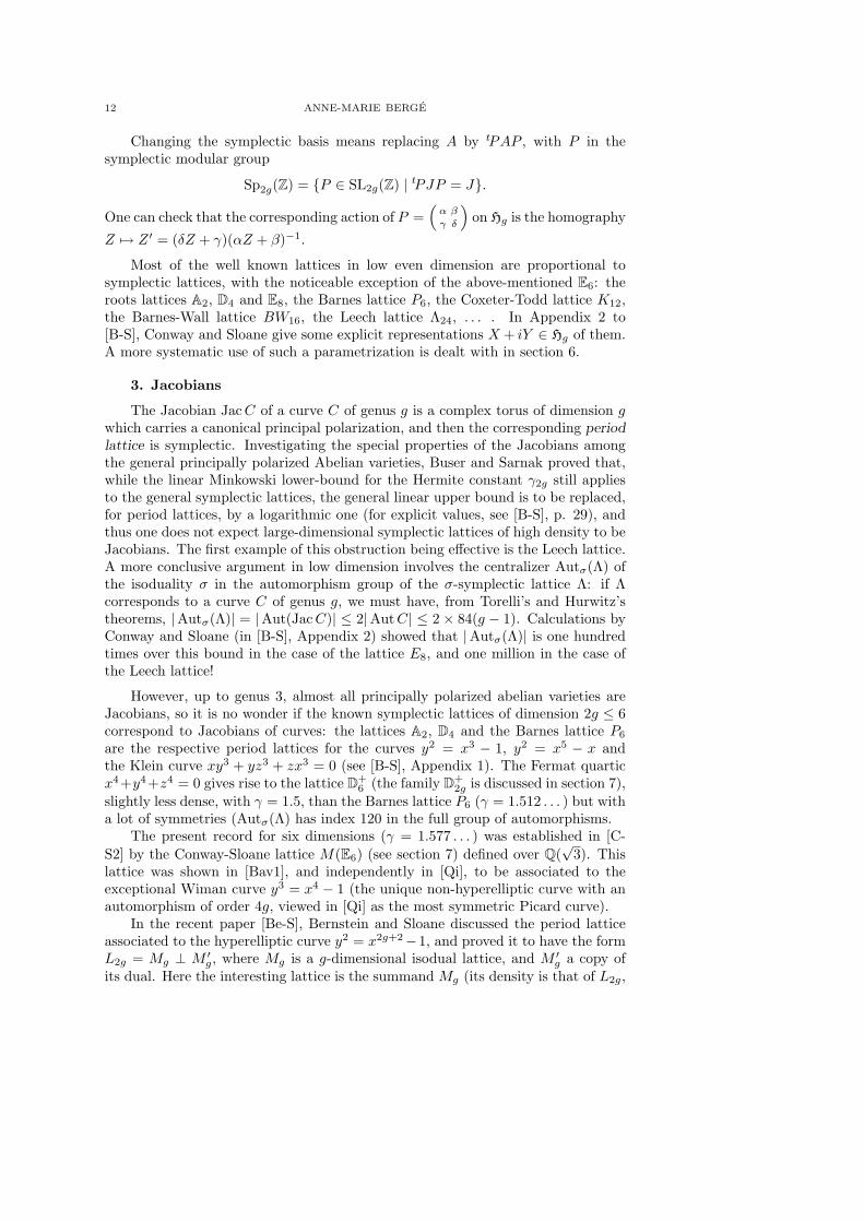
The Jacobian Jac C of a curve C of genus g is a complex torus of dimension gwhich carries a canonical principal polarization, and then the corresponding periodlattice is symplectic. Investigating the special properties of the Jacobians amongthe general principally polarized Abelian varieties, Buser and Sarnak proved that,while the linear Minkowski lower-bound for the Hermite constant γ2g still appliesto the general symplectic lattices, the general linear upper bound is to be replaced,for period lattices, by a logarithmic one (for explicit values, see [B-S], p. 29), andthus one does not expect large-dimensional symplectic lattices of high density to beJacobians. The first example of this obstruction being effective is the Leech lattice.A more conclusive argument in low dimension involves the centralizer Autσ(Λ) ofthe isoduality σ in the automorphism group of the σ-symplectic lattice Λ: if Λcorresponds to a curve C of genus g, we must have, from Torelli’s and Hurwitz’stheorems, |Autσ(Λ)| = |Aut(Jac C)| ≤ 2|Aut C| ≤ 2× 84(g − 1). Calculations byConway and Sloane (in [B-S], Appendix 2) showed that |Autσ(Λ)| is one hundredtimes over this bound in the case of the lattice E8, and one million in the case ofthe Leech lattice!
However, up to genus 3, almost all principally polarized abelian varieties areJacobians, so it is no wonder if the known symplectic lattices of dimension 2g ≤ 6correspond to Jacobians of curves: the lattices A2, D4 and the Barnes lattice P6
are the respective period lattices for the curves y2 = x3 − 1, y2 = x5 − x andthe Klein curve xy3 + yz3 + zx3 = 0 (see [B-S], Appendix 1). The Fermat quarticx4+y4+z4 = 0 gives rise to the lattice D+
6 (the family D+2g is discussed in section 7),
slightly less dense, with γ = 1.5, than the Barnes lattice P6 (γ = 1.512 . . . ) but witha lot of symmetries (Autσ(Λ) has index 120 in the full group of automorphisms.
The present record for six dimensions (γ = 1.577 . . . ) was established in [C-S2] by the Conway-Sloane lattice M(E6) (see section 7) defined over Q(
√3). This
lattice was shown in [Bav1], and independently in [Qi], to be associated to theexceptional Wiman curve y3 = x4 − 1 (the unique non-hyperelliptic curve with anautomorphism of order 4g, viewed in [Qi] as the most symmetric Picard curve).
In the recent paper [Be-S], Bernstein and Sloane discussed the period latticeassociated to the hyperelliptic curve y2 = x2g+2−1, and proved it to have the formL2g = Mg ⊥ M ′
g, where Mg is a g-dimensional isodual lattice, and M ′g a copy of
its dual. Here the interesting lattice is the summand Mg (its density is that of L2g,

SYMPLECTIC LATTICES 13
and its group has only index 2): it turns out to be, for g ≤ 3, the densest isodualpacking in g dimensions.
Remark. The Hermite problem is part of a more general systole problem (see[Bav1]). So far, although a compact Riemann surface is determined by its polarizedJacobian, no connection between its systole and the Hermite invariant of the periodlattice seems to be known.
4. Modular lattices
4.1 Definition. Let Λ be an n-dimensional integral lattice (i.e. Λ ⊂ Λ∗),which is similar to its dual. If σ is a similarity such that σ(Λ∗) = Λ, its norm ` (σmultiplies squared lengths by `) is an integer which does not depend on the choiceof σ. Following Quebbemann, we call Λ a modular lattice of level. Note that levelone corresponds to unimodular lattices.
For a given pair (n, `), the (hypothetical) modular lattices have a prescribed deter-minant `n/2, thus, up to isometry, there are only finitely many of them; as usualwe are looking for the largest possible minimum m (the Hermite invariant γ = m√
`
depends only on it). In the following, we restrict to even dimensions and evenlattices.
Then, the modular properties of the theta series of such lattices yield constraintsfor the dimension and the density analogous to Hecke’s results for ` = 1 ([C-S1],chapter 7). Still, for some aspects of these questions, the unimodular case remainssomewhat special. For example, given a prime `, there exists even `-modular latticesof dimension n if and only if ` ≡ 3 mod 4 or n ≡ 0 mod 4 (see [Q1]).
4.2 Connection with modular forms. Let Λ be an even lattice of minimumm, and let ΘΛ be its theta series
ΘΛ(z) =∑
x∈Λ
q(x.x)/2 = 1 + 2sqm/2 + · · · ( where q = e2πiz).
Now, when Λ is `-modular (` > 1), ΘΛ must be a modular form of weight n/2 withrespect to the so-called Fricke group of level `, a subgroup of SL2(R) which containsΓ0(`) with index 2 (here again, the unimodular case is exceptional).
From the algebraic structure of the corresponding space M of modular forms,Quebbemann derives the notion of extremal modular lattices extending that of[C-S1], chapter 7. Let d = dimM be the dimension of M. If a form f ∈ M isuniquely determined by the first d coefficients a0, a1, · · · , ad−1 of its q-expansionf =
∑k≥0 akqk, the unique form FM = 1 +
∑k≥d akqk is called `. extremal, and
an even `-modular lattice with this theta series is called an extremal lattice. Sucha (hypothetical) extremal lattice has the highest possible minimum, equal to 2dunless the coefficient ad of FM vanishes. No general results about the coefficientsof the extremal modular form and more generally of its eligibility as a theta seriesseem to be known.
4.3 Special levels. Quebbemann proved that the above method is valid inparticular for prime levels ` such that ` + 1 divides 24, namely 2, 3, 5, 7, 11 and23. (For a more general setup, we refer the reader to [Q1], [Q2] and [S-SP].) Thedimension of the space of modular forms is then d = 1 + bn(1+`)
48 c (which reduces

14 ANNE-MARIE BERGE
to Hecke’s result for ` = 1). The proof of the upper bound
m ≤ 2 + 2⌊
n(1 + `)48
⌋
was completed in [S-SP] by R. Scharlau and R. Schulze-Pillot, by investigating thecoefficients ak, k > 0 of the extremal modular form: all of them are even integers,the leading one ad is positive, but ad+1 is negative for n large enough. So, for agiven level in the above list, there are (at most) only finitely many extremal lattices.Other kinds of obstructions may exist.
4.4 Examples.• ` = 7, at jump dimensions (where the minimum may increase) n ≡ 0 mod 6.
While ad+1 first goes negative at n = 30, Scharlau and Hemkemeier proved thatno 7-extremal lattice exists in dimension 12: their method consists in classifyingfor given pairs (n, `) the even lattices Λ of level ` (i.e.
√`Λ∗ is also even) with
detΛ = `n/2; for (n, `) = (12, 7), they found 395 isometry classes, and among themno extremal modular lattice.
If an extremal lattice were to exist for (n, `) = (18, 7), it would set new recordsof density. Bachoc and Venkov proved recently in [B-V2] that no such lattice exists:their proof involves spherical designs.
• Extremal lattices of jump dimensions are specially wanted, since they oftenachieve the best known density, like in the following examples:
Minimum 2. D4 ((n, `) = (4, 2)); E8 ((n, `) = (8, 1)).Minimum 4. K12 ((n, `) = (12, 3)); BW16 ((n, `) = (16, 2)); the Leech lattice
((n, `) = (24, 1)).Minimum 6. (n, `) = (32, 2): 4 known lattices, Quebbemann discovered the
first one (denoted Q32 in [C-S1]) in 1984; (n, `) = (48, 1): 3 known lattices P48p,P48q from coding theory, and a “cyclo-quaternionic” lattice by Nebe.
• Extremal even unimodular lattices are known for any dimension n ≡ 0mod 8, n ≤ 80, except for n = 72, which would set a new record of density. Thecase n = 80 was recently solved by Bachoc and Nebe. The corresponding Hermiteinvariant γ = 8 (largely over the upper bound for period lattices) does not hold thepresent record for dimension 80, established at 8, 0194 independently by Elkies andShioda. The same phenomenon appeared at dimension 56.
We give in section 7 Hermitian constructions for most of the above extremallattices, making obvious their symplectic nature.
5. Voronoi’s theory
5.1 Local theory. In section 4, we looked for extremal lattices, which (if any)maximize the Hermite invariant in the (finite) set of modular lattices for a given pair(n, `). In the present section, we go back to the classical notion of an extreme lattice,where the Hermite invariant γ achieves a local maximum. Here, the existenceof such lattices stems from Mahler’s compactness theorem. The same argumentapplies when we study the local maxima of density in some natural families oflattices such as isodual lattices, lattices with prescribed automorphisms etc. Thesefamilies share a common structure: their connected components are orbits of onelattice under the action of a closed subgroup G of GL(E) invariant under transpose.
SYMPLECTIC LATTICES 15
For such a family F , we can give a unified characterization of the strict local maximaof density. In order to point out the connection with Voronoi’s classical theorem
a lattice is extreme if and only if it is perfect and eutactic,we mostly adopt in the following the point of view of Gram matrices. We denote bySymn(R) the space of n× n symmetric matrices equipped with the scalar product< M,N >= Trace(MN). The value at v ∈ Rn of a quadratic form A is thentvAv =< A, vtv >.
5.2 Perfection, eutaxy and extremality. Let G be a closed subgroup ofSLn(R) stable under transpose, and let F = tPAP,P ∈ G be the orbit of apositive definite matrix A ∈ Symn(R). We denote by TA the tangent space to themanifold F at A, and we recall that S(A) stands for the set of the minimal vectorsof A.
• Let v ∈ Rn. The gradient at A (with respect to <,>) of the function F → R+
A 7→< A, vtv > det A−1/n is the orthogonal projection ∇v = projTA(vtv) of vtv onto
the tangent space at A.
The F-Voronoi domain of A is
DA = convex hull ∇v, v ∈ S(A).We say that A is F-perfect if the affine dimension of DA is maximum (= dim TA),and eutactic if the projection of the matrix A−1 lies in the interior of DA.
These definitions reduce to the traditional ones when we take for F the wholeset of positive n × n matrices (and TA = Symn(R)). But in this survey we focuson families F naturally normalized to determinant 1: the tangent space at A tosuch a family is orthogonal to the line RA−1, and the eutaxy condition reduces to
“0 ∈DA”.
• The matrix A is called F-extreme if γ achieves a local maximum at A amongall matrices in F . We say that A is strictly F-extreme if there is a neighbourhoodV of A in F such that the strict inequality γ(A′) < γ(A) holds for every A′ ∈ V ,A′ 6= A.
• The above concepts are connected by the following result.
Theorem ([B-M]). The matrix A is strictly F-extreme if and only if it isF-perfect and F-eutactic.
The crucial step in studying the Hermite invariant in an individual family F isthen to check the strictness of any local maximum. A sufficient condition is thatany F-extreme matrix should be well rounded, i.e. that its minimal vectors shouldspan the space Rn. It was proved by Voronoi in the classical case.
5.3 Isodual lattices. Let σ be an isometry of E with a given integral repre-sentation S. Then we can parametrize the family of σ-isodual lattices by the Liegroup and symmetrized tangent space at identity
G = P ∈ GLn(R) | tP−1 = SPS−1, TI = X ∈ Symn(R) | SX = −XS.The answer to the question
does σ-extremality imply strict σ-extremality?
16 ANNE-MARIE BERGE
depends on the representation afforded by σ ∈ O(E). It is positive for symplecticor orthogonal lattices. A minimal counter-example is given by a three-dimensionalrotation σ of order 4: the corresponding isodual lattices are decomposable (see[C-S2], th. 1), and the Hermite invariant for this family attains its maximum 1 ona subvariety of dimension 2 (up to isometry).
In [Qi-Z], Voronoi’s condition for symplectic lattices was given a suitable com-plex form. It holds for the Conway and Sloane lattice M(E6) (and of course forthe Barnes lattice P6 which is extreme in the classical sense) but not for the latticeD+
6 . (An alternative proof involving differential geometry was given in [Bav1].)
In dimension 5 et 7, the most likely candidates for densest isodual lattices werealso discovered by Conway and Sloane; they were successfully tested for isodualitiesσ of orthogonal type (of respective signatures (4, 1) and (4, 3)). In dimension 3,Conway and Sloane proved by classification and direct calculation that the so calledm.c.c. isodual lattice is the densest one (actually, there are only 2 well roundedisodual lattices, m.c.c. and the cubic lattice).
5.4 Extreme modular lattices. The classical theory of extreme lattices wasrecently revisited by B. Venkov [Ve] in the setting of spherical designs. That theset of minimal vectors of a lattice be a spherical 2- or 4-design is a strong form ofthe conditions of eutaxy (equal coefficients) or extremality.
An extremal `-modular lattice is not necessarily extreme: the even unimodularlattice E8 ⊥ E8 has minimum 2, hence is extremal, but as a decomposable lattice,it could not be perfect. By use of the modular properties of some theta serieswith spherical coefficients, Bachoc and Venkov proved ([B-V2]) that this phenom-enon could not appear near the “jump dimensions”: in particular, any extremal`-modular lattice of dimension n such that (` = 1, and n ≡ 0, 8 mod 24), or(` = 2, and n ≡ 0, 4 mod 16), or (` = 3, and n ≡ 0, 2 mod 12), is extreme.
This applies to the famous lattices quoted in section 4. [For some of them,alternative proofs of the Voronoi conditions could be done, using the automorphismgroups (for eutaxy), testing perfection modulo small primes, or inductively in thecase of laminated lattices.]
5.5 Classification of extreme lattices. Voronoi established that there areonly finitely many equivalence classes of perfect matrices, and he gave an algorithmfor their enumeration.
Let A be a perfect matrix, and DA its traditional Voronoi domain. It isa polyhedron of maximal dimension N = n(n + 1)/2, with a finite number ofhyperplane faces. Such a face H of DA is simultaneously a face for the domain ofexactly one other perfect matrix, called the neighbour of A across the face H.
We get, in taking the dual polyhedron, a graph whose edges describe the neigh-bouring relations; this graph has finitely many inequivalent vertices. Voronoi provedthat this graph is connected, and he used it up to dimension 5 to confirm the clas-sification by Korkine and Zolotarev. His attempt for dimension 6 was completedin 1957 by Barnes. Complete classification for dimension 7 was done by Jaquet in1991 using this method. Recently implemented by Batut in dimension 8, Voronoi’salgorithm produced, by neighbouring only matrices with s = N, N + 1 and N + 2,exactly 10916 inequivalent perfect lattices. There may exist some more.
This algorithm was extended in [B-M-S] to matrices invariant under a givenfinite group Γ ⊂ GLn(Z)): it works in the centralizer of Γ in Symn(R).

SYMPLECTIC LATTICES 17
That there are only finitely many isodual-extreme lattices of type symplectic ororthogonal stems from their well roundness. But the present extensions of Voronoi’salgorithm are very partial (see section 6).
5.6 Voronoi’s paths and isodual lattices. The densest known isoduallattices discovered by Conway and Sloane up to seven dimensions were found onpaths connecting, in the lattice space, the densest lattice Λ to its dual Λ∗: sucha path turns out to be stable under a fixed duality, and the isodual lattice M(Λ)is the fixed point for this involution. In [C-S2], these paths were constructed bygluing theory.
Actually, the Voronoi algorithm for perfect lattices provides another interpre-tation of them. In dimensions 6 and 7, the densest lattices E6 and E7 and theirrespective duals are Voronoi neighbours of each other. The above mentioned pathsΛ− Λ∗ are precisely the corresponding neighbouring paths. For dimensions 3 and5, we need a group action: for dimension 5, we use the regular representation Γ ofthe cyclic group of order 5, and the path D5−D∗5 contains the Γ-neighbouring pathleading from D5 to the perfect lattice A3
5; for dimension 3, we use the augmentationrepresentation of the cyclic group of order 4, and the Conway and Sloane pathΛ − Λ∗ is part of the Γ-neighbouring path leading from Λ = A3 to the Γ-perfectlattice called “axial centered cuboidal” in [C-S2].
5.7 Eutaxy. The first proof of the finiteness of the set of eutactic lattices (fora given dimension and up to similarity) was given by Ash ([A]) by means of Morsetheory: the Hermite invariant γ is a topological Morse function, and the eutacticlattices are exactly its non-degenerate critical points. Bavard proved in [Bav1] thatγ is no more a Morse function on the space of symplectic lattices of dimension2g ≥ 4; in particular, one can construct continuous arcs of critical points, such asthe following set of symplectic-eutactic 4× 4 matrices
(
I O
O A
), A ∈ SL2(R) s.t. m(A) > 1.
6. Hyperbolic families of symplectic lattices
This section surveys a recent work by Bavard: in [Bav2] he constructs familiesof 2g-dimensional symplectic lattices for which he his able to recover the local andglobal Voronoi theory, as well as Morse’s theory. The convenient frame for theseconstructions is the Siegel space hg = X + iY ∈ Symg(C) | Y > 0, modulohomographic action by the symplectic group Sp2g(Z).
In these families most of the important lattices (E8, K12, BW16, Leech . . . ) andmany others appear with fine Siegel’s representations Z = X + iY .
6.1 Definition.In the following we fix an integral positive symmetric g × g matrix M .
To any complex number z = x + iy, y > 0 in the Poincare upper half plane h, weattach the complex matrix zM = xM + iyM ∈ hg, and we consider the family
F = zM, z ∈ h ⊂ hg.
On can check that the homographic action of(
α β
γ δ
)∈ PSL2(R) on h corresponds
to the homographic action of(
αI βM
γM−1 δI
)∈ Sp2g(R) on F . This last matrix is

18 ANNE-MARIE BERGE
integral when(
α β
γ δ
)lies in a convenient congruence subgroup Γ0(d) of SL2(Z)
(one may take d = detM), thus up to symplectic isometries of lattices, one canrestrict the parameter z to a fundamental domain for Γ0(d) in h.
The symplectic Gram matrix Az associated to z = x+ iy, y > 0 ∈ h, as definedin 2.2, is given by
Az =1y
(M−1 xIxI |z|2M
).
For g = 1 and M a positive integer, this is the general 2 × 2 positive matrixof determinant 1, and we recover the usual representation in h/PSL2(Z) of the2-dimensional lattices.
6.2 Voronoi’s theory. The Voronoi conditions of eutaxy and perfection forthe family F , as defined in 5.2, can be translated in the space h of the parameters,equipped with its Poincare metric ds = |dz|
y .• Fix z ∈ h, and for any v ∈ R2g denote by ∇v the (hyperbolic) gradient at z of
the function z 7→ tvAzv; we can represent the Voronoi domain of Az by the convexhull Dz in C of the ∇v, v ∈ S(Az); it has affine dimension 0, 1 or 2, this maximalvalue means “perfection” for z. As defined in 5.2, z is eutactic if there exist strictlypositive coefficients cv such that
∑v∈S(Az) cv∇v = 0.
Bavard showed that Voronoi’s and Ash’s theories hold for the family F :Strict extremality ⇔ extremality ⇔ perfection and eutaxy,Hermite’s function is a Morse function, its critical points are the eutactic ones.
Actually, these results are connected to the strict convexity of the Hermite functionon the family F (see [Bav1] for a more general setting).
Remark. In the above theory, the only gradients that matter are the extremalpoints of the convex Dz. Following Bavard, we call principal the correspondingminimal vectors. In the classical theory, all minimal vectors are principal; this isno more true in its various extensions.
• The next step towards a global study of γ in F was to get an hyperbolicinterpretation of the values tvAzv. To this purpose, Bavard represents any vectorv ∈ R2g by a point p ∈ h∪∂h in such a way that for all z ∈ h, tvAzv is an exponentialfunction of the hyperbolic distance d(p, z) (suitably extended to the boundary ∂h).In particular, there is a discrete set P corresponding to the principal minimalvectors.
• There is now a simple description of the Voronoi theory for the family F . Weconsider the Dirichlet-Voronoi tiling of the metric space (h, d) attached to the setP: the cell around p is Cp = z ∈ h | d(z, p) ≤ d(z, q) for all q ∈ P.
We then introduce the dual partition: the Delaunay cell of z ∈ h is the convexhull of the points of P closest to z (for the Poincare metric), hence it can figurethe Voronoi domain Dz. As one can imagine, the F-perfect points are the verticesof the Dirichlet-Voronoi tiling, and the F-eutactic points are those which lie in theinterior of their Delaunay cell.
The 1-skeleton of the Dirichlet-Voronoi tiling is the graph of the neighbouringrelation between perfect points. Bavard proved that it is connected, and finitemodulo the convenient congruence subgroup. For a detailed description of thealgorithm, we refer the reader to [Bav2], 1.5 and 1.6.

SYMPLECTIC LATTICES 19
6.3 Some examples.• For M = Dg (g ≥ 3), the algorithm only produces one perfect point z = 1+i
2 ,corresponding to the so-called lattice D+
2g (see next section).• The choice M = Ag, g ≥ 1 is much less disappointing: it produces many
symplectic-extreme lattices, among them A2,D4, P6,E8,K12.• The densest lattices in the families attached to the Barnes lattices M =
Pg, g = 8, 12 are the Barnes-Wall lattice BW16 and the Leech lattice.• However, the union of the hyperbolic families of given dimension 2g has only
dimension g(g + 1)/2 + 1; hence it is no wonder that it misses some beautifulsymplectic lattices, for instance the lattice M(E6).
7. Other constructions
7.1 Hermitian lattices. Let K be a C.M. field or a totally definite quater-nion algebra, and let M be a maximal order of K. All the above-mentioned famouslattices (in even dimensions) can be constructed as M-modules of rank k equippedwith the scalar product trace(αx.y), where trace is the reduced trace K/Q, x.y thestandard Hermitian inner product on R⊗QKk and α ∈ K some convenient totallypositive element (see for example [Bay]). We see in the following examples that sucha construction often provides natural symplectic isodualities and automorphisms.
Lattices D+2g, g ≥ 3. Here M = Z[i] ⊂ C is the ring of Gaussian inte-
gers. We consider in Cg equipped with the scalar product 12 trace(x.y) the lattice
x = (x1, x2, · · · , xg) ∈ Mg | x1 +x2 + · · ·+xg ≡ 0 mod (1+ i) which is isometricto the root lattice D2g. Now we consider the conjugate elements e = 1
1+i (1, 1, · · · , 1)and e (= ie = (1, 1, . . . , 1) − e) of Cg; then the sets D+
2g = D2g ∪ (e + D2g) andD−2g = D2g ∪ (e + D2g) turn out to be dual lattices, that coincide when g is even.In any case, the multiplication by i provides a symplectic isoduality. An obviousgroup of Hermitian automorphisms consist of permutations of the xi’s and evensign changes. Thus, comparing its order 2gg! to the Hurwitz bound (2)84(g − 1),one sees that, except for g = 3, no lattice of the family is a Jacobian (in the oppositedirection, all lattices, except for g = 3, are extreme in the Voronoi sense).
Barnes-Wall lattices BW2k , k ≥ 2. Here, K is the quaternion field Q2,∞defined over Q by elements i, j such that i2 = j2 = −1, ji = −ij, M is the Hurwitzorder (Z-module generated by (1, i, j, ω) where ω = 1/2(1 + i + j + ij)), and weconsider the two-sided ideal A = (1 + i)M of M. Starting from M0 = A, we defineinductively the right and left M-modules
Mk+1 = (x, y) ∈ Mk ×Mk | x ≡ y mod AMk ⊂ K2k+2,
and for k odd (resp. even) we put Lk = Mk (resp. A−1Mk). For the scalar product12 trace(x.y), we have L0 ∼ D4, L1 ∼ E8 and generally Lk ∼ BW22k+2 . Theselattices are alternatively 2-modular and unimodular: the right multiplication byi (resp. j − i) for k odd (resp. k even) provides a symplectic similarity σ fromL∗k = Lk (resp. A−1Lk) onto Lk. Using their logarithmic bound for the density of aperiod lattice, Buser and Sarnak proved that the Barnes-Wall lattices are certainlynot Jacobians for k ≥ 5. As usual, an argument of automorphisms extends thisresult for 1 ≤ k ≤ 4: the group Autσ(Lk) embeds diagonally into Autσ(Lk+2), andadding transpositions and sign changes, one obtains a subgroup of Autσ(Lk+2) oforder 27 ×Autσ(Lk); starting from the subgroup of automorphisms of D4 given by
20 ANNE-MARIE BERGE
left multiplication by the 24 units of M, or from the group Autσ(E8), one sees that|Autσ(Lk)| is largely over the Hurwitz bound.
Hermitian extensions of scalars. Let M the ring of integers of a imaginaryquadratic field. Following [G], Bachoc and Nebe show in [B-N] that by tensoringover M a modular M-lattice, one can shift from one level to another; this construc-tion preserves the symplectic nature of the isoduality, and hopefully, the minimum.For this last question, we refer to [Cou].
In [B-N], M is the ring of integers of the quadratic field of discriminant −7. LetLr be an M-lattice of rank r, unimodular with respect to its Hermitian structure,and consider the M-lattices L2r = (A2 ⊥ A2) ⊗M Lr and L4r = E8 ⊗M Lr. By adeterminant argument, one sees that (for the usual scalar product) the Z-latticesLr, L2r and L4r are symplectic modular lattices of respective levels 7, 3 and 1.Starting from the Barnes lattice P6, Gross obtained the Coxeter-Todd lattice K12
and the Leech lattice, of minimum 4. The same procedure was applied in [B-N] toa 20-dimensional lattice appearing in the ATLAS in connection with the Mathieugroup M22, and led to the first known extremal modular lattices of minimum 8,and respective dimensions 40 and 80. Note that while coding theory was involvedin the original proof of the extremality of the unimodular lattices of dimension 80,an alternative “a la Kitaoka” proof is given in [Cou].
7.2 Exterior power. Let 1 ≤ k < n be two integers, and let E be a Euclideanspace of dimension n; its exterior powers carry a natural scalar product whichmakes the canonical map σ :
∧n−kE → (
∧kE)∗ an isometry
∧n−kE → (
∧kE)
of square (−1)k(n−k). Let L be a lattice in E. It is shown in [Cou1] that σ maps thelattice
∧n−kL onto
√detL(
∧kL)∗. In particular, when n = 2k, σ is a symplectic
or orthogonal similarity of the(2kk
)-dimensional lattice (
∧kL) onto its dual; if
moreover L is integral, the lattice (∧k
L) is modular of level det L.For instance, the lattice
∧2 D4 is isometric to D+6 , and the lattice
∧3 E6, in 20dimensions, is 3-modular of symplectic type, with minimum 4, thus extremal.
Remark. Exterior even powers of unimodular lattices are unimodular latticesof special interest for the theory of group representations. Let us come back to thenotation of this subsection. For even k, the canonical map Aut L → Aut
∧kL has
kernel ±1, and induces an embedding AutL/(±1) → Aut∧k
L. Actually, the exte-rior squares of the lattice E8 and the Leech lattice provide faithful representationsof minimal degrees of the group O+
8 (2) and of the Conway group Co1 respectively.
7.3 Group representations. Many important symplectic modular latticeswere discovered by Nebe, Plesken ([N-P]) and Souvignier ([Sou]) while investigatingfinite rational matrix groups. In [S-T], Scharlau and Tiep, using symplectic groupsover Fp, construct large families of symplectic unimodular lattices, among themthat of dimension 28 discovered by combinatorial devices by Bacher and Venkov in[B-V1].
I am indebted to C. Bavard and J. Martinet for helpful discussions when I waswriting this survey. I am also grateful for the improvements they suggested afterreading the first drafts of this paper.

SYMPLECTIC LATTICES 21
References
[A] A. Ash, On eutactic forms, Can. J. Math. 29 (1977), 1040–1054.[B-N] C. Bachoc, G. Nebe, Extremal lattices of minimum 8 related to the Mathieu group M22,
J. reine angew. Math. 494 (1998), 155–171.[B-V1] R. Bacher, B. Venkov, Lattices and association schemes: a unimodular example without
roots in dimension 28, Ann. Inst. Fourier, Grenoble 45 (1995), 1163–1176.[B-V2] C. Bachoc, B. Venkov, Modular forms, lattices and spherical designs, preprint, Bor-
deaux, 1998.[Bav1] C. Bavard, Systole et invariant d’Hermite, J. reine angew. Math. 482 (1997), 93–120.[Bav2] C. Bavard, Familles hyperboliques de reseaux symplectiques, preprint, Bordeaux, 1997.[Bay] E. Bayer-Fluckiger, Definite unimodular lattices having an automorphism of given
characteristic polynomial, Comment. Math. Helvet. 59 (1984), 509–538.[B-M] A.-M. Berge, J. Martinet, Densite dans des familles de reseaux. Application aux
reseaux isoduaux, L’Enseignement Mathematique 41 (1995), 335–365.[B-M-S] A.-M. Berge, J. Martinet, F. Sigrist, Une generalisation de l’algorithme de Voronoı,
Asterisque 209 (1992), 137–158.[Be-S] M. Bernstein and N.J.A. Sloane, Some lattices obtained from Riemann surfaces, Ex-
tremal Riemann Surfaces, J. R. Quine and P. Sarnak Eds. (Contemporary Math. Vol201), Amer. Math. Soc., Providence, RI, 1997, pp. 29–32.
[B-S] P. Buser, P. Sarnak, On the period matrix of a Riemann surface of large genus (withan Appendix by J.H. Conway and N.J.A. Sloane), Invent. math. 117 (1994), 27–56.
[C-S1] J.H. Conway, N.J.A. Sloane, Sphere Packings, Lattices and Groups, Third edition,Springer-Verlag , Grundlehren 290, Heidelberg, 1999.
[C-S2] J.H. Conway, N.J.A Sloane, On Lattices Equivalent to Their Duals, J. Number Theory48 (1994), 373–382.
[Cou] R. Coulangeon, Tensor products of Hermitian lattices, Acta Arith. 92 (2000), 115–130.[G] B. Gross, Groups over Z, Invent. Math. 124 (1996), 263–279.[M] J. Martinet, Les reseaux parfaits des espaces euclidiens, Masson, Paris, 1996.[M-H] J. Milnor, D. Husemoller, Symmetric Bilinear Forms, Springer-Verlag, Ergebnisse 73,
Heidelberg, 1973.[N-P] G. Nebe, W. Plesken, Finite rational matrix groups, Memoirs A.M.S. 116 (1995),
1–144.[N-V] G. Nebe, B. Venkov, Nonexistence of Extremal Lattices in Certain Genera of Modular
Lattices, J. Number Theory 60 (1996), 310–317.[Q1] H.-G. Quebbemann, Modular Lattices in Euclidean Spaces, J. Number Theory 54
(1995), 190–202.[Q2] H.-G. Quebbemann, Atkin-Lehner eigenforms and strongly modular lattices, L’Ensei-
gnement Mathematique 43 (1997), 55–65.[Qi] J.R. Quine, Jacobian of the Picard Curve, Contemp. Math. 201 (1997).[Qi-Z] J.R. Quine, P. L. Zhang, Extremal Symplectic Lattices, Israel J. Math. 108 (1998),
237–251.[S-T] R. Scharlau, P. H. Tiep, Symplectic group lattices, Trans. Amer. Math. Soc. 351 (1999),
2101–2131.[S-SP] R. Scharlau, R. Schulze-Pillot, Extremal lattices, Algorithmic Algebra and Number
Theory, B.H. Matzat, G.-M. Greul, G. Hiss ed., Springer-Verlag, Heidelberg, 1999,pp. 139–170.
[Sh] T. Shioda, A Collection: Mordell-Weil Lattices, Max-Planck Inst. Math., Bonn (1991).[Sou] B. Souvignier, Irreducible finite integral matrix groups of degree 8 and 10, Math. Comp.
63 (1994), 335–350.[V] G. Voronoı, Nouvelles applications des parametres continus a la theorie des formes
quadratiques : 1 Sur quelques proprietes des formes quadratiques positives parfaites,J. reine angew. Math 133 (1908), 97–178.
[Ve] B. Venkov, notes by J. Martinet, Reseaux et “designs” spheriques, preprint, Bordeaux,1999.
22 ANNE-MARIE BERGE
Institut de MathematiquesUniversite Bordeaux 1351 cours de la Liberation33405 Talence Cedex, France
E-mail address: [email protected]
Contemporary Mathematics
Universal Quadratic Forms and theFifteen Theorem
J. H. Conway
Abstract. This paper is an extended foreword to the paper of ManjulBhargava [1] in these proceedings, which gives a short and elegant proofof the Conway-Schneeberger Fifteen Theorem on the representation ofintegers by quadratic forms.
The representation theory of quadratic forms has a long history, start-ing in the seventeenth century with Fermat’s assertions of 1640 about thenumbers represented by x2 + y2. In the next century, Euler gave proofs ofthese and some similar assertions about other simple binary quadratics, andalthough these proofs had some gaps, they contributed greatly to settingthe theory on a firm foundation.
Lagrange started the theory of universal quadratic forms in 1770 byproving his celebrated Four Squares Theorem, which in current language isexpressed by saying that the form x2+y2+z2+t2 is universal. The eighteenthcentury was closed by a considerably deeper statement – Legendre’s ThreeSquares Theorem of 1798; this found exactly which numbers needed all foursquares. In his Theorie des Nombres of 1830, Legendre also created a verygeneral theory of binary quadratics.
The new century was opened by Gauss’s Disquisitiones Arithmeticae of1801, which brought that theory to essentially its modern state. Indeed,when Neil Sloane and I wanted to summarize the classification theory ofbinary forms for one of our books [3], we found that the only Number Theorytextbook in the Cambridge Mathematical Library that handled every casewas still the Disquisitiones! Gauss’s initial exploration of ternary quadraticswas continued by his great disciple Eisenstein, while Dirichlet started theanalytic theory by his class number formula of 1839.
As the nineteenth century wore on, other investigators, notably H. J. S.Smith and Hermann Minkowski, explored the application of Gauss’s conceptof the genus to higher-dimensional forms, and introduced some invariantsfor the genus from which in this century Hasse was able to obtain a complete
c©0000 (copyright holder)
23
24 J. H. CONWAY
and very simple classification of rational quadratic forms based on Hensel’snotion of “p-adic number”, which has dominated the theory ever since.
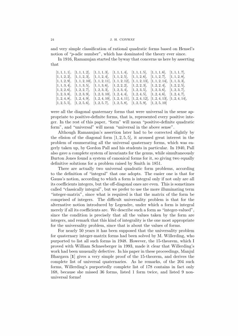
In 1916, Ramanujan started the byway that concerns us here by assertingthat
[1, 1, 1, 1], [1, 1, 1, 2], [1, 1, 1, 3], [1, 1, 1, 4], [1, 1, 1, 5], [1, 1, 1, 6], [1, 1, 1, 7],[1, 1, 2, 2], [1, 1, 2, 3], [1, 1, 2, 4], [1, 1, 2, 5], [1, 1, 2, 6], [1, 1, 2, 7], [1, 1, 2, 8],[1, 1, 2, 9], [1, 1, 2, 10], [1, 1, 2, 11], [1, 1, 2, 12], [1, 1, 2, 13], [1, 1, 2, 14], [1, 1, 3, 3],[1, 1, 3, 4], [1, 1, 3, 5], [1, 1, 3, 6], [1, 2, 2, 2], [1, 2, 2, 3], [1, 2, 2, 4], [1, 2, 2, 5],[1, 2, 2, 6], [1, 2, 2, 7], [1, 2, 3, 3], [1, 2, 3, 4], [1, 2, 3, 5], [1, 2, 3, 6], [1, 2, 3, 7],[1, 2, 3, 8], [1, 2, 3, 9], [1, 2, 3, 10], [1, 2, 4, 4], [1, 2, 4, 5], [1, 2, 4, 6], [1, 2, 4, 7],[1, 2, 4, 8], [1, 2, 4, 9], [1, 2, 4, 10], [1, 2, 4, 11], [1, 2, 4, 12], [1, 2, 4, 13], [1, 2, 4, 14],[1, 2, 5, 5], [1, 2, 5, 6], [1, 2, 5, 7], [1, 2, 5, 8], [1, 2, 5, 9], [1, 2, 5, 10]
were all the diagonal quaternary forms that were universal in the sense ap-propriate to positive-definite forms, that is, represented every positive inte-ger. In the rest of this paper, “form” will mean “positive-definite quadraticform”, and “universal” will mean “universal in the above sense”.
Although Ramanujan’s assertion later had to be corrected slightly bythe elision of the diagonal form [1, 2, 5, 5], it aroused great interest in theproblem of enumerating all the universal quaternary forms, which was ea-gerly taken up, by Gordon Pall and his students in particular. In 1940, Pallalso gave a complete system of invariants for the genus, while simultaneouslyBurton Jones found a system of canonical forms for it, so giving two equallydefinitive solutions for a problem raised by Smith in 1851.
There are actually two universal quadratic form problems, accordingto the definition of “integral” that one adopts. The easier one is that forGauss’s notion, according to which a form is integral only if not only are allits coefficients integers, but the off-diagonal ones are even. This is sometimescalled “classically integral”, but we prefer to use the more illuminating term“integer-matrix”, since what is required is that the matrix of the form becomprised of integers. The difficult universality problem is that for thealternative notion introduced by Legendre, under which a form is integralmerely if all its coefficients are. We describe such a form as “integer-valued”,since the condition is precisely that all the values taken by the form areintegers, and remark that this kind of integrality is the one most appropriatefor the universality problem, since that is about the values of forms.
For nearly 50 years it has been supposed that the universality problemfor quaternary integer-matrix forms had been solved by M. Willerding, whopurported to list all such forms in 1948. However, the 15-theorem, which Iproved with William Schneeberger in 1993, made it clear that Willerding’swork had been unusually defective. In his paper in these proceedings, ManjulBhargava [1] gives a very simple proof of the 15-theorem, and derives thecomplete list of universal quaternaries. As he remarks, of the 204 suchforms, Willerding’s purportedly complete list of 178 contains in fact only168, because she missed 36 forms, listed 1 form twice, and listed 9 non-universal forms!

UNIVERSAL QUADRATIC FORMS AND THE FIFTEEN THEOREM 25
The 15-theorem closes the universality problem for integer-matrix formsby providing an extremely simple criterion. We no longer need a list ofuniversal quaternaries, because a form is universal provided only that itrepresent the numbers up to 15. Moreover, this criterion works for largernumbers of variables, where the number of universal forms is no longer finite.(It is known that no form in three or fewer variables can be universal.)
I shall now briefly describe the history of the 15-theorem. In a 1993Princeton graduate course on quadratic forms, I remarked that a rework-ing of Willerding’s enumeration was very desirable, and could probably beachieved very easily in view of recent advances in the representation theoryof quadratic forms, most particularly the work of Duke and Schultze-Pillot.Moreover, it was an easy consequence of this work that there must be a con-stant c with the property that if a matrix-integral form represented everypositive integer up to c, then it was universal, and a similar but probablylarger constant C for integer-valued forms. At that time, I feared that per-haps these constants would be very large indeed, but fortunately it appearedthat they are quite small.
I started the next lecture by saying that we might try to find c, andwrote on the board a putative
Theorem 0.1. If an integer-matrix form represents every positive inte-ger up to c (to be found!) then it is universal.
We started to prove that theorem, and by the end of the lecture hadfound the 9 ternary “escalator” forms (see Bhargava’s article [1] for theirdefinition) and realised that we could almost as easily find the quaternaryones, and made it seem likely that c was much smaller than we had expected.
In the afternoon that followed, several class members, notably WilliamSchneeberger and Christopher Simons, took the problem further by produc-ing these forms and exploring their universality by machine. These calcula-tions strongly suggested that c was in fact 15.
In subsequent lectures we proved that most of the 200+ quaternarieswe had found were universal, so that when I had to leave for a meetingin Boston only nine particularly recalcitrant ones remained. In Boston Itackled seven of these, and when I returned to Princeton, Schneeberger andI managed to polish the remaining two off, and then complete this to a proofof the 15-theorem, modulo some computer calculations that were later doneby Simons.
The arguments made heavy use of the notion of genus, which had en-abled the nineteenth-century workers to extend Legendre’s Three Squarestheorem to other ternary forms. In fact the 15-theorem largely reduces toproving a number of such analogues of Legendre’s theorem. Expressing thearguments was greatly simplified by my own symbol for the genus, whichwas originally derived by comparing Pall’s invariants with Jones’s canonicalforms, although it has since been established more simply; see for instancemy recent little book [2].

26 J. H. CONWAY
Our calculations also made it clear that the larger constant C for theinteger-valued problem would almost certainly be 290, though obtaining aproof of the resulting “290-conjecture” would be very much harder indeed.Last year, in one of our semi-regular conversations I tempted Manjul Bhar-gava into trying his hand at the difficult job of proving the 290-conjecture.
Manjul started the task by reproving the 15-theorem, and now he hasdiscovered the particularly simple proof he gives in the following paper,which has made it unnecessary for us to publish our rather more complicatedproof. Manjul has also proved the “33-theorem” – much more difficult thanthe 15-theorem – which asserts that an integer-matrix form will represent allodd numbers provided only that it represents 1, 3, 5, 7, 11, 15, and 33. Thisresult required the use of some very clever and subtle arithmetic arguments.
Finally, using these arithmetic arguments, as well as new analytic tech-niques, Manjul has made significant progress on the 290-conjecture, and Iwould not be surprised if the conjecture were to be finished off in the nearfuture! He intends to publish these and other related results in a subsequentpaper.
References
[1] M. Bhargava, On the Conway-Schneeberger Fifteen Theorem, these proceedings.[2] J. H. Conway, The sensual (quadratic) form, Carus Mathematical Monographs 26,
MAA, 1997.[3] J. H. Conway and N. A. Sloane, Sphere packings, lattices and groups, Grundlehren der
Mathematischen Wissenschaften 290, Springer-Verlag, New York, 1999.
Department of MathematicsPrinceton UniversityPrinceton, NJ 08544E-mail address: [email protected]
Contemporary Mathematics
On the Conway-Schneeberger Fifteen Theorem
Manjul Bhargava
Abstract. This paper gives a proof of the Conway-Schneeberger Fif-teen Theorem on the representation of integers by quadratic forms, towhich the paper of Conway [1] in these proceedings is an extended fore-word.
1. Introduction. In 1993, Conway and Schneeberger announced thefollowing remarkable result:
Theorem 1 (“The Fifteen Theorem”). If a positive-definite quadraticform having integer matrix represents every positive integer up to 15 then itrepresents every positive integer.
The original proof of this theorem was never published, perhaps becauseseveral of the cases involved rather intricate arguments. A sketch of thisoriginal proof was given by Schneeberger in [4]; for further background anda brief history of the Fifteen Theorem, see Professor Conway’s article [1] inthese proceedings.
The purpose of this paper is to give a short and direct proof of theFifteen Theorem. Our proof is in spirit much the same as that of the originalunpublished arguments of Conway and Schneeberger; however, we are ableto treat the various cases more uniformly, thereby obtaining a significantlysimplified proof.
2. Preliminaries. The Fifteen Theorem deals with quadratic forms thatare positive-definite and have integer matrix. As is well-known, there is anatural bijection between classes of such forms and lattices having integerinner products; precisely, a quadratic form f can be regarded as the innerproduct form for a corresponding lattice L(f). Hence we shall oscillate freelybetween the language of forms and the language of lattices. For brevity, bya “form” we shall always mean a positive-definite quadratic form havinginteger matrix, and by a “lattice” we shall always mean a lattice havinginteger inner products.
c©0000 (copyright holder)
27

28 MANJUL BHARGAVA
A form (or its corresponding lattice) is said to be universal if it representsevery positive integer. If a form f happens not to be universal, define thetruant of f (or of its corresponding lattice L(f)) to be the smallest positiveinteger not represented by f .
Important in the proof of the Fifteen Theorem is the notion of “escalatorlattice.” An escalation of a nonuniversal lattice L is defined to be any latticewhich is generated by L and a vector whose norm is equal to the truant ofL. An escalator lattice is a lattice which can be obtained as the result of asequence of successive escalations of the zero-dimensional lattice.
3. Small-dimensional Escalators. The unique escalation of the zero-dimensional lattice is the lattice generated by a single vector of norm 1.This lattice corresponds to the form x2 (or, in matrix form, [ 1 ]) which failsto represent the number 2. Hence an escalation of [ 1 ] has inner productmatrix of the form [
1 aa 2
].
By the Cauchy-Schwartz inequality, a2 ≤ 2, so a equals either 0 or ±1. Thechoices a = ±1 lead to isometric lattices, so we obtain only two nonisometrictwo-dimensional escalators, namely those lattices having Minkowski-reducedGram matrices
1 00 1
and
1 00 2
.
If we escalate each of these two-dimensional escalators in the same man-ner, we find that we obtain exactly 9 new nonisometric escalator lattices,namely those having Minkowski-reduced Gram matrices
24
1 0 00 1 00 0 1
35 ,
24
1 0 00 1 00 0 2
35 ,
24
1 0 00 1 00 0 3
35 ,
24
1 0 00 2 00 0 2
35 ,
24
1 0 00 2 00 0 3
35 ,
24
1 0 00 2 10 1 4
35 ,
24
1 0 00 2 00 0 4
35 ,
24
1 0 00 2 10 1 5
35 , and
24
1 0 00 2 00 0 5
35.
Escalating now each of these nine three-dimensional escalators, we findexactly 207 nonisomorphic four-dimensional escalator lattices. All such lat-tices are of the form [1]⊕ L, and the 207 values of L are listed in Table 3.
When attempting to carry out the escalation process just once more,however, we find that many of the 207 four-dimensional lattices do not esca-late (i.e., they are universal). For instance, one of the four-dimensional esca-lators turns out to be the lattice corresponding to the famous four squaresform, a2 + b2 + c2 + d2, which is classically known to represent all inte-gers. The question arises: how many of the four-dimensional escalators areuniversal?
4. Four-dimensional Escalators. In this section, we prove that in fact201 of the 207 four-dimensional escalator lattices are universal; that is tosay, only 6 of the four-dimensional escalators can be escalated once again.

ON THE CONWAY-SCHNEEBERGER FIFTEEN THEOREM 29
The proof of universality of these 201 lattices proceeds as follows. Ineach such four-dimensional lattice L4, we locate a 3-dimensional sublatticeL3 which is known to represent some large set of integers. Typically, wesimply choose L3 to be unique in its genus; in that case, L3 represents allintegers that it represents locally (i.e., over each p-adic ring Zp). Armedwith this knowledge of L3, we then show that the direct sum of L3 with itsorthogonal complement in L4 represents all sufficiently large integers n ≥ N .A check of representability of n for all n < N finally reveals that L4 is indeeduniversal.
To see this argument in practice, we consider in detail the escalations
L4 of the escalator lattice24
1 0 00 2 00 0 2
35 (labelled (4) in Table 1). The latter
3-dimensional lattice L3 is unique in its genus, so a quick local calculationshows that it represents all positive integers not of the form 2e(8k+7), wheree is even. Let the orthogonal complement of L3 in L4 have Gram matrix[m]. We wish to show that L3⊕ [m] represents all sufficiently large integers.
To this end, suppose L4 is not universal, and let u be the first integer notrepresented by L4. Then, in particular, u is not represented by L3, so u mustbe of the form 2e(8k + 7). Moreover, u must be squarefree; for if u = rt2
with t > 1, then r = u/t2 is also not represented by L4, contradicting theminimality of u. Therefore e = 0, and we have u ≡ 7 (mod 8).
Now if m 6≡ 0, 3 or 7 (mod 8), then clearly u − m is not of the form2e(8k + 7). Similarly, if m ≡ 3 or 7 (mod 8), then u − 4m cannot be ofthe form 2e(8k + 7). Thus if m 6≡ 0 (mod 8), and given that u ≥ 4m, theneither u − m or u − 4m is represented by L3; that is, u is represented byL3⊕ [m] (a sublattice of L4) for u ≥ 4m. An explicit calculation shows thatm never exceeds 28, and a computer check verifies that every escalation L4
of L3 represents all integers less than 4 × 28 = 112. It follows that anyescalator L4 arising from L3, for which the value of m is not a multiple of8, is universal.
Of course, the argument fails for those L4 for which m is a multiple of8. We call such an escalation “exceptional”. Fortunately, such exceptionalescalations are few and far between, and are easily handled. For instance, an
explicit calculation shows that only two escalations of L3 =24
1 0 00 2 00 0 2
35 are
exceptional (while the other 24 are not); these exceptional cases are listedin Table 2.1. As is also indicated in the table, although these lattices didescape our initial attempt at proof, the universality of these four-dimensionallattices L4 is still not any more difficult to prove; we simply change the
sublattice L3 from the escalator lattice24
1 0 00 2 00 0 2
35 to the ones listed in the
table, and apply the same argument!

30 MANJUL BHARGAVA
It turns out that all of the 3-dimensional escalator lattices listed in Ta-ble 1, except for the one labeled (6), are unique in their genus, so the univer-sality of their escalations can be proved by essentially identical arguments,with just a few exceptions. As for escalator (6), although not unique in itsgenus, it does represent all numbers locally represented by it except possiblythose which are 7 or 10 (mod 12). Indeed, this escalator contains the lattice24
1 0 00 4 20 2 8
35 , which is unique in its genus, and the lattices
24
2 -2 2-2 5 22 2 8
35 and
24
3 0 00 5 40 4 5
35, which together form a genus; a local check shows that the first
genus represents all numbers locally represented by escalator (6) which arenot congruent to 2 or 3 (mod 4), while the second represents all such num-bers not congruent to 1 (mod 3). The desired conclusion follows. (This facthas been independently proven by Kaplansky [3] using different methods.)
Knowing this, we may now proceed with essentially the same arguments
on the escalations of L3 =24
1 0 00 2 10 1 4
35 . The relevant portions of the proofs
for all nonexceptional cases are summarized in Table 1.“Exceptional” cases arise only for escalators (4) (as we have already
seen), (6), and (7). Two arise for escalator (4). Although four arise forescalator (6), two of them turn out to be nonexceptional escalations of (1)and (8) respectively, and hence have already been handled. Similarly, twoarise for escalator (7), but one is a nonexceptional escalation of (9). Thusonly five truly exceptional four-dimensional escalators remain, and these arelisted in Table 2. In these five exceptional cases, other three-dimensionalsublattices unique in their genus are given for which essentially identicalarguments work in proving universality. Again, all the relevant informationis provided in Table 2.
5. Five-dimensional Escalators. As mentioned earlier, there are 6 four-dimensional escalators which escalate again; they have been italicized inTable 3 and are listed again in the first column of Table 4. A rather largecalculation shows that these 6 four-dimensional lattices escalate to an addi-tional 1630 five-dimensional escalators! With a bit of fear we may ask againwhether any of these five-dimensional escalators escalate.
Fortunately, the answer is no; all five-dimensional escalators are uni-versal. The proof is much the same as the proof of universality of thefour-dimensional escalators, but easier. We simply observe that, for the 6four-dimensional nonuniversal escalators, all parts of the proof of universal-ity outlined in the second paragraph of Section 4 go through—except forthe final check. The final check then reveals that each of these 6 latticesrepresent every positive integer except for one single number n. Hence oncea single vector of norm n is inserted in such a lattice, the lattice must au-tomatically become universal. Therefore all five-dimensional escalators are
ON THE CONWAY-SCHNEEBERGER FIFTEEN THEOREM 31
universal. A list of the 6 nonuniversal four-dimensional lattices, togetherwith the single numbers they fail to represent, is given in Table 4.
Since no five-dimensional escalator can be escalated, it follows that thereare only finitely many escalator lattices: 1 of dimension zero, 1 of dimensionone, 2 of dimension two, 9 of dimension three, 207 of dimension four, and1630 of dimension five, for a total of 1850.
6. Remarks on the Fifteen Theorem. It is now obvious that
(i) Any universal lattice L contains a universal sublattice of dimension atmost five.
For we can construct an escalator sequence 0 = L0 ⊆ L1 ⊆ . . . within L,and then from Sections 4 and 5, we see that either L4 or (when defined) L5
gives a universal escalator sublattice of L.Our next remark includes the Fifteen Theorem.
(ii) If a positive-definite quadratic form having integer matrix represents thenine critical numbers 1, 2, 3, 5, 6, 7, 10, 14, and 15, then it represents everypositive integer.(Equivalently, the truant of any nonuniversal form must be one of these ninenumbers.)
This is because examination of the proof shows that only these numbersarise as truants of escalator lattices.
We note that Remark (ii) is the best possible statement of the FifteenTheorem, in the following sense.
(iii) If t is any one of the above critical numbers, then there is a quaternarydiagonal form that fails to represent t, but represents every other positiveinteger.
Nine such forms of minimal determinant are [2, 2, 3, 4] with truant 1, [1, 3, 3, 5]with truant 2, [1, 1, 4, 6] with truant 3, [1, 2, 6, 6] with truant 5, [1, 1, 3, 7] withtruant 6, [1, 1, 1, 9] with truant 7, [1, 2, 3, 11] with truant 10, [1, 1, 2, 15] withtruant 14, and [1, 2, 5, 5] with truant 15.
However, there is another slight strengthening of the Fifteen Theorem,which shows that the number 15 is rather special:
(iv) If a positive-definite quadratic form having integer matrix representsevery number below 15, then it represents every number above 15.
This is because there are only four escalator lattices having truant 15, andas was shown in Section 5, each of these four escalators represents everynumber greater than 15.
Fifteen is the smallest number for which Remark (iv) holds. In fact:

32 MANJUL BHARGAVA
(v) There are forms which miss infinitely many integers starting from anyof the eight critical numbers not equal to 15.
Indeed, in each case one may simply take an appropriate escalator lattice ofdimension one, two, or three.
(vi) There are exactly 204 universal quaternary forms.
An upper bound for the discriminant of such a form is easily determined;a systematic use of the Fifteen Theorem then yields the desired result. Wenote that the enumeration of universal quaternary forms was announcedpreviously in the well-known work of Willerding [5], who found that thereare exactly 178 universal quaternary forms; however, a comparison with ourtables shows that she missed 36 universal forms, listed one universal formtwice, and listed 9 non-universal forms. A list of all 204 universal quaternaryforms is given in Table 5; the three entries not appearing among the list ofescalators in Table 3 have been italicized.
Acknowledgments. The author wishes to thank Professors Conway andKaplansky for many wonderful discussions, and for helpful comments on anearlier draft of this paper.
References
[1] J. H. Conway, Universal quadratic forms and the Fifteen Theorem, these proceedings.[2] J. H. Conway and N. A. Sloane, Sphere packings, lattices and groups, Grundlehren der
Mathematischen Wissenschaften 290, Springer-Verlag, New York, 1999.[3] I. Kaplansky, The first non-trivial genus of positive definite ternary forms, Math.
Comp. 64 (1995), no. 209, 341–345.[4] W. A. Schneeberger, Arithmetic and Geometry of Integral Lattices, Ph.D. Thesis,
Princeton University, 1995.[5] M. E. Willerding, Determination of all classes of positive quaternary quadratic forms
which represent all (positive) integers, Ph.D. Thesis, St. Louis University, 1948.

ON THE CONWAY-SCHNEEBERGER FIFTEEN THEOREM 33
Three-dimensional Represents nos. Checkescalator lattice Truant not of the form∗ If m Subtract up to
(1)
24
1 0 00 1 00 0 1
35 7 2eu7 6≡ 0 (mod 8) m or 4m 112
≡ 0 (mod 8) does not arise -
(2)
24
1 0 00 1 00 0 2
35 14 2du7 6≡ 0 (mod 16) m or 4m 224
≡ 0 (mod 16) does not arise -
(3)
24
1 0 00 1 00 0 3
35 6 3du− 6≡ 0 (mod 9) m, 4m, or 16m 864
≡ 0 (mod 9) does not arise -
(4)
24
1 0 00 2 00 0 2
35 7 2eu7 6≡ 0 (mod 8) m or 4m 112
≡ 0 (mod 8) [See Table 2] -
(5)
24
1 0 00 2 00 0 3
35 10 2du5 6≡ 0 (mod 16) m or 4m 1440
≡ 0 (mod 16) does not arise -
(6)
24
1 0 00 2 10 1 4
35 7 7du− or 6≡ 0, 3, 9 (mod 12)
7, 10 (mod 12) & 6≡ 0 (mod 49) m, 4m, or 9m 3087
≡ 0 (mod 49) does not arise -
≡ 0, 3, 9 (mod 12) [See Table 2] -
(7)
24
1 0 00 2 00 0 4
35 14 2du7 6≡ 0 (mod 16) m or 4m 224
≡ 0 (mod 8) [See Table 2] -
(8)
24
1 0 00 2 10 1 5
35 7 2eu7 6≡ 0 (mod 8) m or 4m 252
≡ 0 (mod 8) does not arise -
(9)
24
1 0 00 2 00 0 5
35 10 5du− 6≡ 0 (mod 25) m or 4m 4000
≡ 0 (mod 25) does not arise -
Table 1. Proof of universality of four-dimensional escalators(nonexceptional cases)

34 MANJUL BHARGAVA
“Exceptional” New unique in Unrepresented CheckLattice genus sublattice numbers m Subtract up to
2664
1 0 0 20 2 0 10 0 2 12 1 1 7
3775
24
1 0 00 2 10 1 3
35 5du+ 40 m or 4m 160
2664
1 0 0 00 2 0 10 0 2 10 1 1 7
3775
24
2 0 10 2 11 1 7
35 2eu1, 2
eu5,
2du3, 2du7, 3
du+1 m 14
2664
1 0 0 10 2 1 00 1 4 31 0 3 7
3775
24
2 1 11 4 01 0 4
35 2du7 1 m, 4m, or 9m 9
2664
1 0 0 00 2 1 10 1 4 00 1 0 7
3775
† 24
2 0 00 4 20 2 10
35 2du7 90 m or 4m 504
2664
1 0 0 10 2 0 00 0 4 21 0 2 14
3775
24
1 0 00 4 20 2 13
35 2du5, 2
eu3 2 m or 4m 8
Table 2. Proof of universality of four-dimensional escalators (exceptional cases)
∗We follow the notation of Conway-Sloane [2]: pd (resp. pe) denotes an odd (resp.even) power of p; if p = 2, uk denotes a number of the form 8n + k (k = 1, 3, 5, 7), and ifp is odd, u+ (resp. u−) denotes a number which is a quadratic residue (resp. non-residue)modulo p.
†In this exceptional case, the sublattice given here shows only that all even numbersare represented. However, the original argument of Table 1 (using escalator (6) as sublat-tice, with m = 315) shows that all odd numbers are represented, so the desired universalityfollows. [It turns out there is no sublattice unique in its genus that single-handedly provesuniversality in this case!]

ON THE CONWAY-SCHNEEBERGER FIFTEEN THEOREM 35
1: 1 1 1 0 0 0 16: 2 3 3 2 0 0 30: 2 4 4 2 0 0 49: 2 3 9 2 2 0 72: 2 5 8 4 0 0
2: 1 1 2 0 0 0 17: 1 2 9 2 0 0 31: 2 3 6 2 2 0 49: 2 4 7 0 0 2 74: 2 4 10 2 2 0
3: 1 1 3 0 0 0 17: 1 3 6 2 0 0 31: 2 4 5 0 2 2 49: 2 5 6 0 2 2 76: 2 4 10 0 2 0
3: 1 2 2 2 0 0 17: 2 3 4 0 2 2 32: 2 4 4 0 0 0 50: 2 4 7 2 2 0 77: 2 5 9 4 2 0
4: 1 1 4 0 0 0 18: 1 2 9 0 0 0 32: 2 4 5 4 0 0 50: 2 5 5 0 0 0 78: 2 4 10 2 0 0
4: 1 2 2 0 0 0 18: 1 3 6 0 0 0 33: 2 3 6 0 2 0 51: 2 3 9 0 2 0 78: 2 5 8 2 0 0
4: 2 2 2 2 2 0 18: 2 2 5 2 0 0 33: 2 4 5 2 0 2 52: 2 3 9 2 0 0 80: 2 4 10 0 0 0
5: 1 1 5 0 0 0 18: 2 3 3 0 0 0 34: 2 3 6 2 0 0 52: 2 5 6 2 0 2 80: 2 4 11 4 0 0
5: 1 2 3 2 0 0 18: 2 3 4 2 0 2 34: 2 4 5 2 2 0 52: 2 5 6 4 0 0 80: 2 5 8 0 0 0
6: 1 1 6 0 0 0 19: 1 2 10 2 0 0 34: 2 4 6 4 0 2 53: 2 5 6 2 2 0 82: 2 4 11 2 2 0
6: 1 2 3 0 0 0 19: 2 3 4 2 2 0 35: 2 4 5 0 0 2 54: 2 3 9 0 0 0 82: 2 5 9 4 0 0
6: 2 2 2 2 0 0 20: 1 2 10 0 0 0 36: 2 3 6 0 0 0 54: 2 4 7 2 0 0 83: 2 5 9 2 2 0
7: 1 1 7 0 0 0 20: 2 2 5 0 0 0 36: 2 4 5 0 2 0 54: 2 5 6 0 0 2 85: 2 5 9 0 2 0
7: 1 2 4 2 0 0 20: 2 2 6 2 2 0 36: 2 4 6 4 2 0 54: 2 5 7 4 2 2 86: 2 4 11 2 0 0
7: 2 2 3 2 0 2 20: 2 4 4 4 2 0 36: 2 5 5 4 2 2 55: 2 3 10 2 2 0 87: 2 5 10 4 2 0
8: 1 2 4 0 0 0 21: 2 3 4 0 2 0 37: 2 5 5 4 2 0 55: 2 5 6 0 2 0 88: 2 4 11 0 0 0
8: 1 3 3 2 0 0 22: 1 2 11 0 0 0 38: 2 4 5 2 0 0 55: 2 5 7 4 0 2 88: 2 4 12 4 0 0
8: 2 2 2 0 0 0 22: 2 2 6 2 0 0 38: 2 4 6 0 2 2 56: 2 4 7 0 0 0 88: 2 5 9 2 0 0
8: 2 2 3 2 2 0 22: 2 3 4 2 0 0 39: 2 3 7 0 2 0 56: 2 4 8 4 0 0 90: 2 4 12 2 2 0
9: 1 2 5 2 0 0 22: 2 3 5 0 2 2 40: 2 3 7 2 0 0 57: 2 3 10 0 2 0 90: 2 5 9 0 0 0
9: 1 3 3 0 0 0 23: 1 2 12 2 0 0 40: 2 4 5 0 0 0 58: 2 3 10 2 0 0 92: 2 4 13 4 2 0
9: 2 2 3 0 0 2 23: 2 3 5 2 0 2 40: 2 4 6 2 0 2 58: 2 4 8 2 2 0 92: 2 5 10 4 0 0
10: 1 2 5 0 0 0 24: 1 2 12 0 0 0 40: 2 4 6 4 0 0 58: 2 5 6 2 0 0 93: 2 5 10 2 2 0
10: 2 2 3 2 0 0 24: 2 2 6 0 0 0 41: 2 4 7 4 0 2 58: 2 5 7 0 2 2 94: 2 4 12 2 0 0
10: 2 2 4 2 0 2 24: 2 2 7 2 2 0 42: 2 3 7 0 0 0 60: 2 3 10 0 0 0 95: 2 5 10 0 2 0
11: 1 2 6 2 0 0 24: 2 3 4 0 0 0 42: 2 4 6 0 0 2 60: 2 4 9 4 2 0 96: 2 4 12 0 0 0
11: 1 3 4 2 0 0 24: 2 4 4 0 2 2 42: 2 4 6 2 2 0 60: 2 5 6 0 0 0 96: 2 4 13 4 0 0
12: 1 2 6 0 0 0 24: 2 4 4 4 0 0 42: 2 5 5 4 0 0 61: 2 5 7 2 0 2 98: 2 4 13 2 2 0
12: 1 3 4 0 0 0 25: 1 2 13 2 0 0 43: 2 3 8 2 2 0 62: 2 4 8 2 0 0 98: 2 5 10 2 0 0
12: 2 2 3 0 0 0 25: 2 3 5 2 2 0 43: 2 5 5 2 0 2 62: 2 5 7 4 0 0 100: 2 4 13 0 2 0
12: 2 2 4 0 0 2 26: 1 2 13 0 0 0 44: 2 4 6 0 2 0 63: 2 5 7 0 0 2 100: 2 4 14 4 2 0
13: 2 2 5 2 0 2 26: 2 2 7 2 0 0 45: 2 4 7 0 2 2 63: 2 5 7 2 2 0 100: 2 5 10 0 0 0
13: 2 3 3 2 2 0 26: 2 4 4 2 2 0 45: 2 5 5 0 2 0 64: 2 4 8 0 0 0 102: 2 4 13 2 0 0
14: 1 2 7 0 0 0 27: 1 2 14 2 0 0 45: 2 5 6 4 2 2 66: 2 4 9 2 2 0 104: 2 4 13 0 0 0
14: 1 3 5 2 0 0 27: 2 3 5 0 2 0 46: 2 3 8 2 0 0 67: 2 5 8 4 2 0 104: 2 4 14 4 0 0
14: 2 2 4 2 0 0 27: 2 4 5 4 0 2 46: 2 4 6 2 0 0 68: 2 4 9 0 2 0 106: 2 4 14 2 2 0
15: 1 2 8 2 0 0 28: 1 2 14 0 0 0 46: 2 5 6 4 0 2 68: 2 4 10 4 2 0 108: 2 4 14 0 2 0
15: 1 3 5 0 0 0 28: 2 2 7 0 0 0 47: 2 4 7 2 0 2 68: 2 5 7 2 0 0 110: 2 4 14 2 0 0
15: 2 2 5 0 0 2 28: 2 3 5 2 0 0 47: 2 5 6 4 2 0 70: 2 4 9 2 0 0 112: 2 4 14 0 0 0
15: 2 3 3 0 2 0 28: 2 4 4 0 2 0 48: 2 3 8 0 0 0 70: 2 5 7 0 0 0
16: 1 2 8 0 0 0 28: 2 4 5 4 2 0 48: 2 4 6 0 0 0 72: 2 4 9 0 0 0
16: 2 2 4 0 0 0 30: 2 3 5 0 0 0 48: 2 5 5 2 0 0 72: 2 4 10 4 0 0
Table 3. Ternary forms‡ L such that [1]⊕ L is an escalator.(The six entries not appearing in Table 5 have been italicized.)
‡We use the customary shorthand “D: a b c d e f” to represent the three-dimensional
lattice
24
a f/2 e/2f/2 b d/2e/2 d/2 c
35 of determinant D.

36 MANJUL BHARGAVA
Nonuniversal four-dimensional escalator Unique number not represented
1 0 0 00 2 0 10 0 3 00 1 0 4
10
1 0 0 00 2 1 00 1 4 10 0 1 5
10
1 0 0 00 2 0 00 0 5 10 0 1 5
15
1 0 0 00 2 0 00 0 5 00 0 0 5
15
1 0 0 00 2 0 10 0 5 20 1 2 8
15
1 0 0 00 2 0 10 0 5 10 1 1 9
15
Table 4. Nonuniversal four-dimensional escalator lattices.(The 1630 five-dimensional escalators are obtained from these.)

ON THE CONWAY-SCHNEEBERGER FIFTEEN THEOREM 37
1: 1 1 1 0 0 0 16: 1 2 8 0 0 0 28: 2 3 5 2 0 0 48: 2 3 8 0 0 0 72: 2 4 9 0 0 0
2: 1 1 2 0 0 0 16: 2 2 4 0 0 0 28: 2 4 4 0 2 0 48: 2 4 6 0 0 0 72: 2 4 10 4 0 0
3: 1 1 3 0 0 0 16: 2 3 3 2 0 0 28: 2 4 5 4 2 0 48: 2 5 5 2 0 0 72: 2 5 8 4 0 0
3: 1 2 2 2 0 0 17: 1 2 9 2 0 0 30: 2 3 5 0 0 0 49: 2 3 9 2 2 0 74: 2 4 10 2 2 0
4: 1 1 4 0 0 0 17: 1 3 6 2 0 0 30: 2 4 4 2 0 0 49: 2 4 7 0 0 2 76: 2 4 10 0 2 0
4: 1 2 2 0 0 0 17: 2 3 4 0 2 2 31: 2 3 6 2 2 0 49: 2 5 6 0 2 2 77: 2 5 9 4 2 0
4: 2 2 2 2 2 0 18: 1 2 9 0 0 0 31: 2 4 5 0 2 2 50: 2 4 7 2 2 0 78: 2 4 10 2 0 0
5: 1 1 5 0 0 0 18: 1 3 6 0 0 0 32: 2 4 4 0 0 0 51: 2 3 9 0 2 0 78: 2 5 8 2 0 0
5: 1 2 3 2 0 0 18: 2 2 5 2 0 0 32: 2 4 5 4 0 0 52: 2 3 9 2 0 0 80: 2 4 10 0 0 0
6: 1 1 6 0 0 0 18: 2 3 3 0 0 0 33: 2 3 6 0 2 0 52: 2 5 6 2 0 2 80: 2 4 11 4 0 0
6: 1 2 3 0 0 0 18: 2 3 4 2 0 2 34: 2 3 6 2 0 0 52: 2 5 6 4 0 0 80: 2 5 8 0 0 0
6: 2 2 2 2 0 0 19: 1 2 10 2 0 0 34: 2 4 5 2 2 0 53: 2 5 6 2 2 0 82: 2 4 11 2 2 0
7: 1 1 7 0 0 0 19: 2 3 4 2 2 0 34: 2 4 6 4 0 2 54: 2 3 9 0 0 0 82: 2 5 9 4 0 0
7: 1 2 4 2 0 0 20: 1 2 10 0 0 0 35: 2 4 5 0 0 2 54: 2 4 7 2 0 0 85: 2 5 9 0 2 0
7: 2 2 3 2 0 2 20: 2 2 5 0 0 0 36: 2 3 6 0 0 0 54: 2 5 6 0 0 2 86: 2 4 11 2 0 0
8: 1 2 4 0 0 0 20: 2 2 6 2 2 0 36: 2 4 5 0 2 0 54: 2 5 7 4 2 2 87: 2 5 10 4 2 0
8: 1 3 3 2 0 0 20: 2 3 4 0 0 2 36: 2 4 6 4 2 0 55: 2 3 10 2 2 0 88: 2 4 11 0 0 0
8: 2 2 2 0 0 0 20: 2 4 4 4 2 0 36: 2 5 5 4 2 2 55: 2 5 6 0 2 0 88: 2 4 12 4 0 0
8: 2 2 3 2 2 0 22: 1 2 11 0 0 0 37: 2 5 5 4 2 0 55: 2 5 7 4 0 2 88: 2 5 9 2 0 0
9: 1 2 5 2 0 0 22: 2 2 6 2 0 0 38: 2 4 5 2 0 0 56: 2 4 7 0 0 0 90: 2 4 12 2 2 0
9: 1 3 3 0 0 0 22: 2 3 4 2 0 0 38: 2 4 6 0 2 2 56: 2 4 8 4 0 0 90: 2 5 9 0 0 0
9: 2 2 3 0 0 2 22: 2 3 5 0 2 2 39: 2 3 7 0 2 0 57: 2 3 10 0 2 0 92: 2 4 13 4 2 0
10: 1 2 5 0 0 0 23: 1 2 12 2 0 0 40: 2 3 7 2 0 0 58: 2 3 10 2 0 0 92: 2 5 10 4 0 0
10: 2 2 3 2 0 0 23: 2 3 5 2 0 2 40: 2 4 5 0 0 0 58: 2 4 8 2 2 0 93: 2 5 10 2 2 0
10: 2 2 4 2 0 2 24: 1 2 12 0 0 0 40: 2 4 6 2 0 2 58: 2 5 6 2 0 0 94: 2 4 12 2 0 0
11: 1 2 6 2 0 0 24: 2 2 6 0 0 0 40: 2 4 6 4 0 0 58: 2 5 7 0 2 2 95: 2 5 10 0 2 0
11: 1 3 4 2 0 0 24: 2 2 7 2 2 0 41: 2 4 7 4 0 2 60: 2 3 10 0 0 0 96: 2 4 12 0 0 0
12: 1 2 6 0 0 0 24: 2 3 4 0 0 0 42: 2 3 7 0 0 0 60: 2 4 9 4 2 0 96: 2 4 13 4 0 0
12: 1 3 4 0 0 0 24: 2 4 4 0 2 2 42: 2 4 6 0 0 2 60: 2 5 6 0 0 0 98: 2 4 13 2 2 0
12: 2 2 3 0 0 0 24: 2 4 4 4 0 0 42: 2 4 6 2 2 0 61: 2 5 7 2 0 2 98: 2 5 10 2 0 0
12: 2 2 4 0 0 2 25: 1 2 13 2 0 0 42: 2 5 5 4 0 0 62: 2 4 8 2 0 0 100: 2 4 13 0 2 0
12: 2 3 3 0 2 2 25: 2 3 5 0 0 2 43: 2 3 8 2 2 0 62: 2 5 7 4 0 0 100: 2 4 14 4 2 0
13: 2 2 5 2 0 2 25: 2 3 5 2 2 0 44: 2 4 6 0 2 0 63: 2 5 7 0 0 2 100: 2 5 10 0 0 0
13: 2 3 3 2 2 0 26: 1 2 13 0 0 0 45: 2 4 7 0 2 2 63: 2 5 7 2 2 0 102: 2 4 13 2 0 0
14: 1 2 7 0 0 0 26: 2 2 7 2 0 0 45: 2 5 5 0 2 0 64: 2 4 8 0 0 0 104: 2 4 13 0 0 0
14: 1 3 5 2 0 0 26: 2 4 4 2 2 0 45: 2 5 6 4 2 2 66: 2 4 9 2 2 0 104: 2 4 14 4 0 0
14: 2 2 4 2 0 0 27: 1 2 14 2 0 0 46: 2 3 8 2 0 0 68: 2 4 9 0 2 0 106: 2 4 14 2 2 0
15: 1 2 8 2 0 0 27: 2 3 5 0 2 0 46: 2 4 6 2 0 0 68: 2 4 10 4 2 0 108: 2 4 14 0 2 0
15: 1 3 5 0 0 0 27: 2 4 5 4 0 2 46: 2 5 6 4 0 2 68: 2 5 7 2 0 0 110: 2 4 14 2 0 0
15: 2 2 5 0 0 2 28: 1 2 14 0 0 0 47: 2 4 7 2 0 2 70: 2 4 9 2 0 0 112: 2 4 14 0 0 0
15: 2 3 3 0 2 0 28: 2 2 7 0 0 0 47: 2 5 6 4 2 0 70: 2 5 7 0 0 0
Table 5. Ternary forms L such that [1]⊕ L is universal.(The three entries not appearing in Table 3 have been italicized.)
Department of Mathematics,Princeton University,Princeton, NJ 08544E-mail address: [email protected]
Contemporary Mathematics
On Trace Forms and the Burnside Ring
Martin Epkenhans
Abstract. We discuss the annihilating polynomials of trace forms arising inthe literature. An improvement of these results is obtained by using a reductionto 2-groups. In several cases we determine the minimal monic annihilatingpolynomial of trace forms with given Galois action.
1. Introduction
Let L/K be a finite separable field extension, with char(K) 6= 2. Let N be anormal closure of L/K and let G = G(N/K) be the Galois group of N/K. We areinterested in a (monic) polynomial p(X) ∈ Z[X] of minimal degree, depending onlyon the Galois action of G on the set of left cosets of G/G(N/L), such that p(X)annihilates the trace form of L/K in the Witt ring W (K) of K.
During the last decade several examples of annihilating polynomials have ap-peared in the literature. First D. Lewis [Lew87] defined a monic polynomial Ln(X)which annihilates any quadratic form of dimension n. Hence there exists a monicannihilating polynomial of minimal degree in our situation. P.E. Conner [Con87]gave a polynomial of lower degree which annihilates trace forms. Beaulieu andPalfrey [BP97] and recently Lewis and McGarraghy [LM00] recover these resultsby giving annihilating polynomials which divide the corresponding Beaulieu-Palfreypolynomials. In [Epk98] we defined a polynomial q(X), called the signature polyno-mial, which divides any annihilating polynomial. Further, there exists some integere ≥ 0 such that 2eq(X) is an annihilating polynomial. Since the only torsion in theWitt ring is 2-torsion, we more like to get monic polynomials.
In this paper we discuss all these polynomials. We show that the Lewis-McGarraghy result improves the Beaulieu-Palfrey theorem. We improve the Lewis-McGarraghy theorem on trace forms of field extensions by using Springer’s theoremon the lifting of quadratic forms to odd degree extensions.
In section 3 we give several examples which show that all the definitions ofannihilating polynomials are essentially different.
In some cases we are able to give a further improvement by using some explicitcalculations of the trace ideal T (G) of the Burnside ring B(G) of G.
Unfortunately we are not able to present a unified approach which yields aminimal monic annihilating polynomial. In section 5.2 we give an example of a
1991 Mathematics Subject Classification. 11E04.
c©0000 (copyright holder)
39
40 MARTIN EPKENHANS
group G acting transitively on a set S such that the signature polynomial is not anannihilating polynomial.
2. The Polynomials
We start by defining the different annihilating polynomials arising in the liter-ature. The first polynomial is given by D. Lewis in [Lew87].
2.1. The Lewis polynomial Ln(X).
Definition 2.1. For n ∈ N the Lewis polynomial is defined as
Ln(X) = X(X2 − 22)(X2 − 42) . . . (X2 − n2) if n is even,Ln(X) = (X2 − 12)(X2 − 32) . . . (X2 − n2) if n is odd.
Theorem 2.2. Let ψ be a quadratic form of dimension n over the field K.Then
Ln(ψ) = 0 ∈ W (K)in the Witt ring W (K) of K.
Observe, that the zeros of Ln(X) are exactly those integers which arise assignatures of quadratic forms of dimension n.
We now restrict our attention to trace forms. Let A be an etale K-algebra ofdimension n over the field K of characteristic 6= 2. Then
A → K : x 7→ traceA/Kx2
defines a quadratic form of dimension n over K, called the trace form of A/K. Wedenote the trace form by < A/K > or simply by < A > if no confusion can arise.We know by Sylvester and Jacobi that trace forms have non-negative signatures.
2.2. The Conner polynomial Cn(X).
Definition 2.3. For n ∈ N the Conner polynomial Cn(X) is defined to be
Cn(X) = X(X − 2)(X − 4) . . . (X − n) if n is even,Cn(X) = (X − 1)(X − 3) . . . (X − n) if n is odd.
Hence Cn(X) =∏
k≥0,Ln(k)=0(X − k) is the positive part of Ln(X). Fromunpublished notes of P.E. Conner [Con87] we get
Theorem 2.4. Let L/K be a separable field extension of degree n. Then
Cn(< L >) = 0 ∈ W (K).
The results of Lewis and Conner are optimal in the following sense. Let M bea class of quadratic forms. Then
IM = f ∈ Z[X] : f(ψ) = 0 ∈ W (K) for all ψ ∈ Mis the vanishing ideal of M . Regarding the signatures of quadratic forms we observethe following result. Ln(X) generates the principal ideal IQn , where Qn containsall quadratic forms of dimension n. Let Tn be the class of trace forms of dimensionn of fields of characteristic 6= 2. Then ITn = (Cn(X)) (see [Epk98]). Hence thesignatures are the only obstructions.
Let L/K be separable field extension of degree n. Choose a normal closureN ⊃ L of L/K. Denote the Galois group of N/K by G(N/K) and set H = G(N/L).Let f(X) ∈ K[X] be a polynomial with L ' K[X]/(f). Then the transitive action

ON TRACE FORMS AND THE BURNSIDE RING 41
of G on the roots of f(X) is equivalent to the faithful action of G on the set of leftcosets of H in G. Instead of fixing a field extension L/K we choose a finite groupG and a subgroup H < G such that the action
G×G/H → G/H
is faithful. We know that the action is transitive. Further G acts faithfully if andonly if ∩σ∈GσHσ−1 = 1 if and only if H contains no subgroup 6= 1 which is normalin G.
Definition 2.5. Let H < G be finite groups with ∩σ∈GσHσ−1 = 1. LetM(G,H) denotes the class of all quadratic forms ψ such that there is an irreducibleand separable polynomial f(X) ∈ K[K] with Galois group Gal(f) ' G and suchthat
(1) the action of Gal(f) on the roots of f(X) is equivalent to the action of Gon G/H, and
(2) ψ and the trace form of K[X]/(f(X)) over K are isometric.
We look for a polynomial mG,H(X) ∈ Z[X] such that mG,H(X) annihilates anyquadratic form in M(G,H). Actually we are interested in a (monic) polynomial ofminimal degree with the property cited above.
Beaulieu and Palfrey [BP97] gave an annihilating polynomial which dividesConner’s polynomial. In general their polynomial has smaller degree.
2.3. The Beaulieu-Palfrey polynomial BG,H(X). Let G be a finite groupacting on a finite set S. For σ ∈ G let χ(σ) = ]Sσ be the number of fixed point ofσ acting on S. Then the Galois number tG,S is defined to be the maximum valueof 1 + χ(σ) as σ runs over all elements of G which do not act as the identity on S.Beaulieu and Palfrey proved the following theorem.
Theorem 2.6. Let G be a finite group and let H < G be a subgroup with∩σ∈GσHσ−1 = 1. Let t = tG,H denote the Galois number of the action of G onG/H. Set
BG,H(X) = (X − n)t−1∏
k=0,k≡0 mod 2
(X − k),
where n = [G : H]. Then BG,H(X) annihilates any ψ ∈ M(G,H).
In [EG99] we find a complete list of the Galois numbers of all doubly transitivepermutation groups. Let us give some examples and consequences. We get Cn(X) =Bn(X) in the case of the symmetric group Sn acting on n letters.
A Frobenius group G of degree n has Galois number 2. Hence the Beaulieu-Palfrey polynomial is X − n, if n is odd and X(X − n) if n is even.
Recently Lewis and McGarraghy [LM00] gave an annihilating polynomial fortrace forms which divides the Beaulieu-Palfrey polynomial.
2.4. The Lewis-McGarraghy polynomial pG,H(X). Again let a finite groupG act on a finite set S. For any subgroup U < G let
SU = s ∈ S : sσ = s for all σ ∈ Ube the set of fixed points of U . Set ϕU (S) = ]SU .

42 MARTIN EPKENHANS
Definition 2.7. Let the finite group G act on set S. Let n = ]S and set
ϕ(S) = ϕU (S) : U < G, ϕU (S) ≡ 0 mod 2.Now define
pG,S =∏
k∈ϕ(S)
(X − k).
Set pG,H = pG,G/H .
The result of Lewis and McGarraghy is as follows.
Theorem 2.8. Let A = K[X]/(f(X)) be an etale K-algebra. Consider theaction of the Galois group G of f(X) on the set S of roots of f(X). Then pG,S(X)annihilates the trace form < A >.
As we will see, this theorem improves the Beaulieu-Palfrey result in two direc-tions. It also holds for etale algebras and, as we see later, there are examples wherethe degree of pG,S(X) is strictly smaller then the degree of BG,H(X). Observe thefollowing. Let σ ∈ G be a non-identity element. Then χ(σ) = ϕ<σ>(S). FurtherϕU (S) ≤ χ(σ) for all σ ∈ U . Hence pG,S(X) divides BG,H(X) and the maximalroot 6= n of both polynomials coincide.
2.5. The dyadic annihilating polynomials B(2)G,H(X)and p
(2)G,H(X). The
proofs of the trace form results cited above are in two steps. Consider the Burnsidering B(G) of G. Let χH be an element defined by the subgroup H < G. First wehave to find a polynomial g(X) ∈ Z[X] such that g(χH) = 0. Let N/K be a Galoisextension with Galois group isomorphic to G. Then there is a homomorphismhN/K : B(G) → W (K) which maps χH onto < NH >. Hence g(X) annihilates thetrace form of the fixed field NH of H over K. By the fact that there are no non-trivial zero divisors of odd degree in W (K), we can omit several roots of g(X). Wecall it the even-odd trick. Hence the results of Conner, Beaulieu-Palfrey, and Lewis-McGarraghy follow from identities in the Burnside ring via a ring homomorphismtogether with the even-odd trick.
Next we show that we get better results by using Springer’s theorem on thelifting of quadratic forms according to odd degree extensions.
Definition 2.9. Let G be a finite group and let H < G be a subgroup of indexn such that ∩σ∈GσHσ−1 = 1. Let G2 be a Sylow 2-group of G. Let t = tG2,G/H
be the Galois number of the action of G2 on G/H. Set
B(2)G,H(X) = (X − n)
t−1∏
k=0,k≡n mod 2
(X − k)
andp(2)G,H = pG2,G/H(X) =
∏
k∈ϕ(G/H)
(X − k),
where ϕ(G/H) = ϕU (G/H) : U < G2.Observe, that ϕU (G/H) ≡ n mod 2 for any 2-group U . Hence the application
of the even-odd trick in this situation does not yield polynomials of lower degree.

ON TRACE FORMS AND THE BURNSIDE RING 43
Theorem 2.10. Consider the situation of theorem 2.6 and set H = G(N/L).We get
B(2)G,H(< L >) = p
(2)G,H(< L >) = 0 ∈ W (K).
.
Proof. As above, we see that p(2)G,H(X) divides B
(2)G,H(X). Let F be the fixed
field of G2 in N . Then < L/K > lifts to the trace form of an etale algebra overF . By [LM00] p
(2)G,H(X) annihilates < L/K > ⊗KF in W (F ). Since F/K has odd
degree, we are done by Springer’s theorem [Sch85][I.5.5.9]. ¤Next we define a polynomial which turns out to divide any annihilating poly-
nomial.
2.6. The signature polynomial qG,H(X). We are interested in an optimalannihilating polynomial. In [Epk98] we defined the following polynomial. Let Gact on S. For any σ ∈ G with σ2 = 1 let signσ(S) = ]Sσ be the signature of Sdefined by the involution σ. Set
qG,S(X) =∏
k∈signσ(S):σ∈G,σ2=1(X − k).
For S = G/H set qG,H(X) = qG,S . In [Epk98] we proved
Theorem 2.11. Let H, G be as above. Then
IM(G,H) ⊂ (qG,H(X)).
There exists some integer e ≥ 0, which only depends on G and H, such that
(2eqG,H(X)) ⊂ IM(G,H).
We call ]Sσ a signature, since this value corresponds to signatures of traceforms via the homomorphism hN/K .
3. The main result on annihilating polynomials
In this section we analyze the known vanishing results.
Theorem 3.1. Let G be a finite group with Sylow 2-group G2 and let H < Gbe a subgroup of index n with ∩σ∈GσHσ−1 = 1. Then
qG,H(X) | pG,H(X) | BG,H(X) | Cn(X) | Ln(X)
andqG,H(X) | p(2)
G,H(X) | B(2)G,H(X).
All polynomials except the signature polynomial qG,H(X) are contained in IM(G,H).There are examples, where qG,H(X) /∈ IM(G,H). In general, these polynomials aredifferent.
We already proved the results on the divisibility of the polynomials. In section5.2 we give an example with qG,H(X) /∈ IM(G,H).
Cn(X) and Ln(X) are different by definition. Since the maximal root 6= n ofCn(X) is n− 2 we get
Lemma 3.2. BG,H(X) = Cn(X) if and only if G contains a transposition.
In [EG99] we find a lot of example with tG,H ≤ n− 3. As already mentionedabove, BG,H has degree ≤ 2 if G is a Frobenius group.

44 MARTIN EPKENHANS
Lemma 3.3. Let H < G be finite groups with ∩σ∈GσHσ−1 = 1.(1) Let [G : H] be odd. If G acts doubly transitive, then
X − 1 | p(2)G,H(X).
(2) Let [G : H] be even. Then X | p(2)G,H(X).
X | qG,H(X) if and only if G contains an involution which is not conjugateto any element in H.
Hence p(2)G,H(X) 6= qG,H(X) if [G : H] 6≡ ]H ≡ 1 mod 2. And X 6 |qG,H(X) if G
contains only one class of involutions and H has even order. The Ree group R(q)and any group with cyclic or generalized quaternion Sylow 2-group contain onlyone conjugacy class of involutions.
Proof. 1. A two point stabilizer does not contain a Sylow 2-group. HenceϕG2(G/H) = 1.2. A one point stabilizer contains a Sylow 2-group of G if and only if H has oddindex in G. Hence ϕG2(G/H) = 0. Now see corollary 11 in [Epk99]. ¤
We now prove that the Lewis-McGarraghy result improves the Beaulieu-Palfreytheorem.
Proposition 3.4. Let R(q) =2 G2(q), q = 32n+1, where n ≥ 1 be the Ree group.Consider R(q) in its doubly transitive representation of degree q3 + 1. Let H be aone-point stabilizer. Then
B(2)G,H(X) = BG,H(X) = (X − n) ·
q+1∏
k=0,k≡0 mod 2
(X − k),
qG,H(X) = (X − (q + 1)) · (X − (q3 + 1)),
pG,H(X) = X(X − 2) · qG,H(X),
p(2)G,H(X) = X · qG,H(X).
FurtherIM(G,H) = (qG,H).
Proof. See [HB82][XI 13.2] for some basic facts on the Ree group. By[EG99][proposition 17] the Galois number is q + 2. Further q + 1 is the num-ber of fixed points of a non-trivial involution in R(q). This gives the result forboth Beaulieu-Palfrey polynomials B
(2)G,H(X), BG,H(X). Since all involutions are
conjugate in R(q), qG,H(X) has degree 2. By lemma 3.3 X divides p(2)G,H .
Now let V < R(q) be a subgroup with ϕV (S) ≥ 3, where S = G/H. Then Vis contained in the stabilizer of three letters, which has order 2. Hence ϕV (S) = nif V = 1 and ϕV (S) = q + 1 otherwise.
Finally, let V be the stabilizer of two letters. Then ϕV (S) = 2, since V hasorder q − 1 6= 2. Since 0 ≡ q3 + 1 ≡ 2 ≡ q + 1 ≡ n mod 2, the even-odd trickdoes not reduce the number of roots. We later prove that qG,H(X) is already anannihilating polynomial (see proposition 4.3). ¤
Recently, McGarraghy found some other examples which show that the Lewis-McGarraghy-polynomial improves the Beaulieu-Palfrey result. Let us give anotherexample.

ON TRACE FORMS AND THE BURNSIDE RING 45
Proposition 3.5. Let G = AGL(n, q), n ≥ 2 be the affine linear group over Fq.Consider the action of G on the vector space V = Fn
q by semilinear transformationsand let H = G0 be the stabilizer of the zero vector. Then H = GL(n, q). We get
B(2)G,H(X) = BG,H(X) = (X − qn) ·
qn−1∏
k=0,k≡q mod 2
(X − k).
If q is odd, then
p(2)G,H(X) = pG,H(X) = qG,H(X) =
n∏
k=0
(X − qk).
If q is even, we get
p(2)G,H(X) = pG,H(X) = X ·
n∏
k=1
(X − qk)
and
qG,H(X) = X ·n∏
k=1,2k≥n
(X − qk).
Proof. Let U < G be a subgroup with ϕU (V ) ≥ 1. We can assume that Uis a subgroup of G0 = GL(n, q). Hence the set of fixed points of U in V is theintersection of all eigenspaces of the eigenvalue 1 of all φ ∈ U . Therefore ϕU (V ) isa power of q.
For any k = 0, . . . , n there is a linear map σ ∈ GL(n, q) which has 1 as aneigenvalue of geometric multiplicity qk. If q is odd, choose the diagonal matrixEk ⊕ (−En−k).
Let q be even. Then x 7→ x + t(1, . . . , 1) is a fixed point free involution. Fork = 2, . . . , n set
Jk =
1 1 0
0. . . . . .
.... . . . . . 1
0 . . . 0 1
∈ Mk(Fq)
and Bk = Jk ⊕En−k. Then Bk is an element of 2-power order having qn−k+1 fixedpoints. Any involution has a Jordan matrix of the form r · J2 ⊕ En−2r. ¤
It remains to give an example with B(2)G,H(X) 6= BG,H(X). Note that B
(2)G,H(X) =
BG,H(X) if and only if the Galois number tG,H is given by an involution.
Proposition 3.6. Let G be a doubly transitive permutation group acting onF6
3 with a one point stabilizer H = G0 ' SL(2, 13). Then
BG,H(X) = (X − 36)4∏
k=0
(X − (2k + 1)),
pG,H(X) = (X − 36)(X − 9)(X − 1),
B(2)G,H(X) = (X − 36)(X − 1) = p
(2)G,H(X) = qG,H .
HenceIM(G,H) = (qG,H).

46 MARTIN EPKENHANS
Proof. A two point stabilizer has order 3. Hence any non-trivial involutionhas exactly one fixed point. By proposition 9 in [EG99] the Galois number equals10. ¤
The next example is due to Pierre Conner.
Proposition 3.7. Let G be a group of odd order and let H be a non trivialsubgroup with ∩σ∈GσHσ−1 = 1. Then
qG,H = p(2)G,H(X) = B
(2)G,H(X) = (X − n) 6= pG,H(X), BG,H(X).
Proof. Observe, that tG,H ≥ 2, if H 6= 1. Now see [Epk98] proposition 4. ¤
4. The trace ideal
4.1. Definitions and basic properties. To make further progress on anni-hilating polynomials we introduce the Burnside ring B(G) and the trace ideal T (G)of a finite group G (see [Epk98], [Epk99], [Hup98][p. 159]). We briefly recall thedefinitions. For any subgroup H of G let χH = χG
H denote the character inducedby the representation of G on the left cosets of H.
Definition 4.1. The Burnside ring B(G) is a free abelian group. The set
χH : H runs over a set of representatives of conjugacy classes of subgroups of Gis a free set of generators of B(G). The multiplication is induced by the tensorproduct of the underlying representations. Hence
χH · χU =⊕
σ∈H\G/U
χH∩σUσ−1 .
Let σ ∈ G be an element with σ2 = 1. The number of fixed points signσχH =ϕ<σ>(G/H) of σ on G/H is called the signature of χH . This definition extends bylinearity to a ring homomorphism signσ : B(G) → Z. Let
L(G) = ∩σ∈G,σ2=1ker(signσ)
be the kernel of the total signature homomorphism.Now let N/K be a Galois extension with Galois group G(N/K) ' G. Then
there is a unique homomorphism
hN/K : B(G) → W (K) : hN/K(χH) =< NH >
(see [Dre71], [BP97], [Epk98], [Epk99]). Now the trace ideal T (G) in B(G) isdefined to be the intersection of all kernels of homomorphisms hN/K , where N/Kruns over all Galois extensions with Galois group ' G of fields of characteristic6= 2. From [Epk99] theorem 6 we know that L(G)/T (G) is a finite 2-group. Wecalculated several examples in [Epk98], [Epk99]. Now we focus our attention onthe polynomial qG,H(X).
Proposition 4.2. Let H < G be finite groups with ∩σ∈GσHσ−1 = 1. Then
qG,H(χH) ∈ L(G).
If G has even order, then deg(qG,H(X)) ≥ 2.
Proof. The roots of qG,H(X) are by definition the possible signature values ofhN/K(χH) =< NH > . Any non-identity involution σ does not act as the identityon G/H. Hence signσχH 6= [G : H] = sign1χH . ¤

ON TRACE FORMS AND THE BURNSIDE RING 47
We now illustrate how the concept of the trace ideal yields an optimal annihi-lating polynomial in some cases.
Proposition 4.3. Let G be a finite group with Sylow 2-group G2 6= 1. Let Hbe a subgroup with ∩σ∈GσHσ−1 = 1. Suppose, that any subgroup of G2 is normalin G2 and that L(G2)/T (G2) has exponent 2. Then
qG,H(χGH) ∈ T (G)
HenceIM(G,H) = (qG,H(X)).
Proof. We prove that the image of qG,H(χGH) under the restriction homomor-
phismresG
G2: B(G) → B(G2)
lies in the trace ideal T (G2). By lemma 4 [Epk98]
resGG2
(qG,H(χGH)) = qG,H(resG
G2(χG
H)) ∈ L(G2).
Since L(G2)/T (G2) has exponent 2, the ideal T (G2) is, regarded as a submodule ofL(G2), given by a system of linear equations modulo 2. Hence it remains to considerthe coefficients of resG
G2(qG,H(χG
H)) modulo 2. From signσχGH ≡ [G : H] mod 2 we
get
resGG2
(qG,H(χGH)) ≡ qG,H(resG
G2(χG
H))
≡ (resGG2
(χGH)− [G : H]χG2
G2)d mod 2B(G2),
where d = deg(qG,H). Let
resGG2
(χGH) =
∑
σ∈G2\G/H
χG2G2∩σHσ−1 =
∑
U<G2
mUχG2U .
Then mG2 = ϕG2(G/H) ≡ [G : H] mod 2. By assumption any subgroup U < G2 isnormal in G2. Therefore (χG2
U )2 = [G2 : U ]χG2U , which implies
(resGG2
(χGH)− [G : H]χG2
G2)2 ≡
∑
U 6=G2
m2U (χG2
U )2 ≡∑
U 6=G2
mU [G2 : U ]χG2U
≡ 0 mod 2 · B(G2).
By proposition 4.2 d ≥ 2. ¤
As an application we get IM(G,H) = (qG,H) in proposition 3.4, since the Sylow2-group of R(q) is an elementary abelian group of order 8. Now use proposition 6[Epk98].
The assumption of the proposition above holds if G2 is cyclic, or elementaryabelian or a direct product of two cyclic groups. These examples yield the question.
Is L(G2)/T (G2) elementary abelian if G2 is abelian?
4.2. A finiteness theorem. In this section we prove that T (G) is an inter-section of finitely many kernels of homomorphisms hN/K , where the field extensionscan chosen to consist of Hilbertian fields.
Lemma 4.4. For any finite group G there exists a finite set M of Galois exten-sions N/K with Galois group G(N/K) ' G such that
T (G) = ∩N/K∈Mker(hN/K).
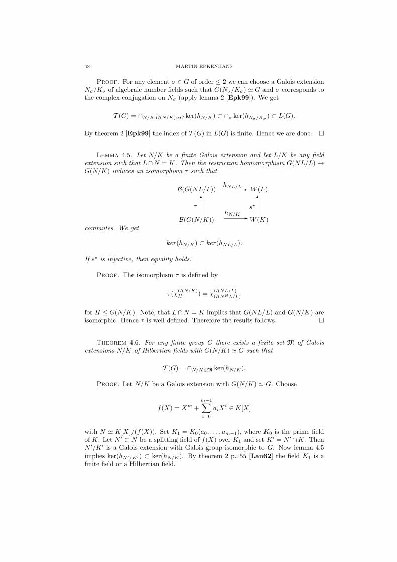
48 MARTIN EPKENHANS
Proof. For any element σ ∈ G of order ≤ 2 we can choose a Galois extensionNσ/Kσ of algebraic number fields such that G(Nσ/Kσ) ' G and σ corresponds tothe complex conjugation on Nσ (apply lemma 2 [Epk99]). We get
T (G) = ∩N/K,G(N/K)'G ker(hN/K) ⊂ ∩σ ker(hNσ/Kσ) ⊂ L(G).
By theorem 2 [Epk99] the index of T (G) in L(G) is finite. Hence we are done. ¤
Lemma 4.5. Let N/K be a finite Galois extension and let L/K be any fieldextension such that L∩N = K. Then the restriction homomorphism G(NL/L) →G(N/K) induces an isomorphism τ such that
B(G(NL/L)) -hNL/L W (L)
W (K)
τ s?
B(G(N/K))
6 6
-hN/K
commutes. We get
ker(hN/K) ⊂ ker(hNL/L).
If s? is injective, then equality holds.
Proof. The isomorphism τ is defined by
τ(χG(N/K)H ) = χ
G(NL/L)
G(NHL/L)
for H ≤ G(N/K). Note, that L ∩N = K implies that G(NL/L) and G(N/K) areisomorphic. Hence τ is well defined. Therefore the results follows. ¤
Theorem 4.6. For any finite group G there exists a finite set M of Galoisextensions N/K of Hilbertian fields with G(N/K) ' G such that
T (G) = ∩N/K∈M ker(hN/K).
Proof. Let N/K be a Galois extension with G(N/K) ' G. Choose
f(X) = Xm +m−1∑
i=0
aiXi ∈ K[X]
with N ' K[X]/(f(X)). Set K1 = K0(a0, . . . , am−1), where K0 is the prime fieldof K. Let N ′ ⊂ N be a splitting field of f(X) over K1 and set K ′ = N ′ ∩K. ThenN ′/K ′ is a Galois extension with Galois group isomorphic to G. Now lemma 4.5implies ker(hN ′/K′) ⊂ ker(hN/K). By theorem 2 p.155 [Lan62] the field K1 is afinite field or a Hilbertian field.
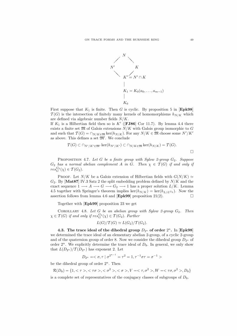
ON TRACE FORMS AND THE BURNSIDE RING 49
N
K ′ = N ′ ∩K
K1 = K0(a0, . . . , am−1)
K0
N ′ K
¡¡
@@
@@
¡¡
First suppose that K1 is finite. Then G is cyclic. By proposition 5 in [Epk98]T (G) is the intersection of finitely many kernels of homomorphisms hN/K whichare defined via algebraic number fields N/K.If K1 is a Hilbertian field then so is K ′ ([FJ86] Cor 11.7). By lemma 4.4 thereexists a finite set M of Galois extensions N/K with Galois group isomorphic to Gand such that T (G) = ∩N/K∈M ker(hN/K). For any N/K ∈ M choose some N ′/K ′
as above. This defines a set M′. We conclude
T (G) ⊂ ∩N ′/K′∈M′ ker(hN ′/K′) ⊂ ∩N/K∈M ker(hN/K) = T (G).
¤
Proposition 4.7. Let G be a finite group with Sylow 2-group G2. SupposeG2 has a normal abelian complement A in G. Then χ ∈ T (G) if and only ifresG2
G (χ) ∈ T (G2).
Proof. Let N/K be a Galois extension of Hilbertian fields with G(N/K) 'G2. By [Mat87] IV.3 Satz 2 the split embedding problem defined by N/K and theexact sequence 1 −→ A −→ G −→ G2 −→ 1 has a proper solution L/K. Lemma4.5 together with Springer’s theorem implies ker(hN/K) = ker(hL/LG2 ). Now theassertion follows from lemma 4.6 and [Epk99] proposition 21(2). ¤
Together with [Epk99] proposition 23 we get
Corollary 4.8. Let G be an abelian group with Sylow 2-group G2. Thenχ ∈ T (G) if and only if resG2
G (χ) ∈ T (G2). Further
L(G)/T (G) ' L(G2)/T (G2).
4.3. The trace ideal of the dihedral group D2n of order 2n. In [Epk98]we determined the trace ideal of an elementary abelian 2-group, of a cyclic 2-groupand of the quaternion group of order 8. Now we consider the dihedral group D2n oforder 2n. We explicitly determine the trace ideal of D8. In general, we only showthat L(D2n)/T (D2n) has exponent 2. Let
D2n =< σ, τ | σ2n−1= τ2 = 1, τ−1στ = σ−1 >
be the dihedral group of order 2n. Then
R(D8) = 1, < τ >, < τσ >,< σ2 >, < σ >, V =< τ, σ2 >,W =< τσ, σ2 >,D8is a complete set of representatives of the conjugacy classes of subgroups of D8.

50 MARTIN EPKENHANS
Proposition 4.9. We get
T (D8) = χ =∑
U∈R(D8)
mUχU : χ ∈ L(G),m<τ> ≡ m<τσ> ≡ 0 mod 2.
Proof. Let
χ = mGχG + mτχ<τ> + mσ2χ<σ2> + mτσχ<τσ>
+mσχ<σ> + mV χV + mW χW + m1χ1 ∈ T (D8).
The system of linear equations defining L(D8) is given by
mG +2mV +2mW +2mσ +4mτ +4mσ2 +4mτσ +8m1 = 0mG +2mV +2mτ = 0mG +2mV +2mW +2mσ +4mσ2 = 0mG +2mW +2mτσ = 0
Let N/K be a Galois extension with G(N/K) ' D8. Set Lτ := N<τ>. There is anirreducible polynomial f = X4 + aX2 + b ∈ K[X] such that N is the splitting fieldof f over K. Assume a 6= 0. The relevant intermediate fields of N/K and theirtrace forms are as follows
H NH < NH >G K < 1 >< τ > K(α) < 1, a2 − 4b,−2a,−2ab(a2 − 4b) >
< σ2 > K(√
b,√
a2 − 4b) 2× < 1, b(a2 − 4b) >
< τσ > K(√
b,√
2√
b− a) < 1, b,−a,−ab(a2 − 4b) >
< σ > K(√
b(a2 − 4b)) < 2, 2b(a2 − 4b) >
V K(√
a2 − 4b) < 2, 2(a2 − 4b) >
W K(√
b) < 2, 2b >< id > N 2× < 1, b(a2 − 4b),−a,−ab(a2 − 4b) >
Calculating the image of χ in W (K) we get
hN/K(χ) = mτσ× < 1,−2 > ⊗ < b > ⊗ < 1,−ab,−a(a2 − 4b),−b(a2 − 4b) > .
If mτσ is even, then mτσ× < 1,−2 >= 0. Consider the generic situation: K =Q(X1, X2), f = X4 + X1X
2 + X2. Then Gal(f) ' D8. Further
ψ =< 1,−X1X2,−X1(X21 − 4X2),−X2(X2
1 − 4X2) >
does not represents 2. Hence < 1,−2 > ⊗ψ 6= 0. The case f = X4 + b is left to thereader. ¤
Proposition 4.10. Let n ≥ 2. Then L(D2n)/T (D2n) is an elementary abelian2-group.
Proof. By proposition 6 [Epk98] and by proposition 4.9 we can assume n ≥ 4.We only give a sketch of the proof. Set G = D2n , V =< τ, σ2 >, χτ = χG
<τ>, χτσ =χG
<τσ>, χσ = χG<σ> and χV = χG
V . We easily observe, that the following set B ofelements in B(D2n) defines a basis of L(D2n).
X1 =χ1 − 2χτ + 2χV − 2χσ ∈ B.
Xτσ =χτσ − χτ + 2χV − χσ − 2χG ∈ B.
For any cyclic group U ⊂< σ2 >,U 6= 1 set
XU =χU − [G : U ]2
χσ ∈ B.

ON TRACE FORMS AND THE BURNSIDE RING 51
If U ⊂< τ, σ4 > is a non-cyclic group, set
XU =χU − χ2 − [G : U ]− 22
χσ ∈ B.
If U 6= G is a non-cyclic subgroup with τσ ∈ U , set
XU =χU − [G : U ]2
χσ + χV − 2χG ∈ B.
Now we have to prove 2χ ∈ T (D2n) for any χ ∈ B. This follows by induction usingcorollary 4 [DEK97] and a fact from the theory of embedding problems which werecall now (Theorem 6 [Kim90]).
Let a, b ∈ K?, such that a, b, ab are not squares in K? and such the qua-dratic forms < 1, b > and < a, ab > are isometric. Set Θ = a +
√a. Then
L = K(√
a,√
b,√
2qΘ), q ∈ K? parametrizes the D8-extensions which contain√a,√
b and which are cyclic over K(√
b). Further L/K is contained in a D16 exten-sion, which is cyclic over K(
√b) if and only if < 1,−2,−a, 2a >'< 1,−q, b,−qb >.
We get< K(
√2qΘ) >'< 1, a, qa, qab >'< 1, a, q, qb > .
2×< 1,−2,−a, 2a >= 0 = 2×< 1,−q, b,−qb > implies 2×< 1, b >' 2×< q, qb > .Hence 2× < K(
√2qθ) >' 2× < 1, 1, a, b >, if K(
√2qθ) is contained in a D16-
extension. The case b = −1 in [Kim90] has to be treated separately. ¤
5. Some applications
5.1. Groups with dihedral Sylow 2-group. The complete classification ofgroups with dihedral Sylow 2-group can be found in [Gor68][16.3].
Proposition 5.1. Let G be a finite group with Sylow 2-group a dihedral groupof order 2n ≥ 8. Then for any subgroup H < G with ∩σ∈GσHσ−1 = 1 we get
IM(G,H) = (qG,H(X)).
Proof. Let n = 3. Since L(D8)/T (D8) has exponent 2, we only have toconsider the coefficients of resG
G2(qG,H(χG
H)) modulo 2. Let
resGG2
(χGH) =
∑
U∈R(D8)
mUχG2U .
We get qG,H(X) ≡ (X − [G : H])d mod F2[X], where d = deg(qG,H(X)). Weknow that mG2 is the number of fixed points of the action of G2 on G/H. HencemG2 ≡ [G : H] mod 2. Therefore
χ = (resGG2
(χGH)− [G : H]χG2
G2)2 ≡
∑
U∈R(D8),U 6=G2
m2U (χG2
U )2 mod 2B(G).
For any normal subgroup U we get (χG2U )2 = [G : U ]χG2
U . Hence
χ ≡ m2τ (χG2
τ )2 + m2τσ(χG2
τσ )2 ≡ mτ (2χG2τ + χG2
1 ) + mτσ(2χG2τσ + χG2
1 )
≡ (mτ + mτσ)χG21 ≡ 0 mod 2B(G),
since mτ ≡ mτσ mod 2 for any element in L(D8). Since d = 2, 3, 4, we are done.Now consider n ≥ 4. Then χ =
∑aUχG2
U +2χ, where U runs over all nontrivialcyclic subgroups of < σ2 >. Further χ ∈ B(G2). Let U, V ∈ G2 be non-trivialsubgroups of G2 such that U is normal in G2 and V 6= G. Then χG2
U ·χG2V ∈ 2B(G2).

52 MARTIN EPKENHANS
We conclude χ · (resGG2
(χGH) − [G : H]χG2
G2) ∈ 2 · B(G2). Hence we are done if
d = deg(qG,H(X)) ≥ 3.Let d = 2. Observe, that a1 is even. By corollary 4 [DEK97] χU ≡ [G2:U ]
2 χG2σ mod
T (G2) for any U ⊂< σ2 >,U 6= 1. Hence resGG2
(qG,H(χGH)) = 2rχG2
σ + 2χ + ˜χ,
where r ∈ Z, ˜χ ∈ T (G2) ⊂ L(G2). Therefore rχG2σ + χ ∈ L(G2). ¤
5.2. Groups with quaternion Sylow 2-group. The aim of this section isto give an example where qG,H(X) does not annihilate < L >. Let us first recallthe determination of the trace ideal of the quaternion group Q8 of order 8. By[Epk98] proposition 7 we get
Proposition 5.2.
T (Q8) = χ =∑
H<Q8
mHχH : χ ∈ L(Q8), mH1 ≡ mH2 ≡ mH3 mod 4 for all
subgroups H1,H2,H3 of order 4 in Q8.Proposition 5.3. Let G be a finite group with Sylow 2-group G2 a quaternion
group of order 8. Let H be a subgroup of G such that G acts faithfully on G/H.Set n := [G : H] and s := signσχG
H . Then
IM(G,H) = (qG,H(X)) = ((X − n)(X − s))
if one of the following cases occur
(1) H is of odd order.(2) ]H ≡ 2 mod 4.(3) ]H ≡ 0 mod 4 and the permutation representation defined by G on G/H
contains only even permutations.
Proof. Since G2 has a unique involution σ we get
qG,H(X) = (X − n)(X − s).
We will prove resG2G (qG,H(χG
H)) ∈ T (G2) in the cases cited above. By proposition5.2 we have to determine the coefficients of χG2
Hiin resG2
G (qG,H(χGH)). Let
resG2G (χG
H) = aχG2G2
+ cχG2σ + dχG2
1 +3∑
i=1
biχG2Hi
.
Since all subgroups of G2 are normal we get
χG2U χG2
V = [G2 : V ]χG21 if U ⊂ V
χG2Hi
χG2Hj
= χG2σ if i 6= j.
Hence
resG2G (qG,H(χG
H)) = a′χG2G2
+ c′χG2σ + d′χG2
1 +3∑
i=1
bi(2bi + 2a− n− s)χG2Hi
.
Further bi = ]τ ∈ G2\G/H : G2 ∩ τHτ−1 = Hi. Hence b1 = b2 = b3 = 0 if]H 6≡ 0 mod 4.

ON TRACE FORMS AND THE BURNSIDE RING 53
Now suppose ]H ≡ 0 mod 4. We get s = signσχGH = a + 2b1 + 2b2 + 2b3 + 4c ≡
n mod 8. Hence s+n2 ≡ n mod 4. Let i 6= j. Then
bi(2bi + 2a− n− s)− bj(2bj + 2a− n− s)
= 2(bi − bj)(bi + bj + a +s + n
2)
≡ 0 mod 4
if and only if (bi − bj)(bi + bj + a + n) is even. Since a ≡ n mod 2, we have todetermine the parity of b1, b2, b3. Let σi be a generator of Hi. The action of G2 onG/H has the following types of orbits:
order of orbit number of orbits isotropy group1 a G2
2 bi Hi
4 c < σ >8 d 1
Hence the sign of σi regarded as a permutation on G/H equals (−1)bj+bk , wherei, j, k = 1, 2, 3. ¤
Observe, that G contains an odd permutation if and only if σi is odd for somei = 1, 2, 3. Now we would like to consider the following situation:
]H ≡ 0 mod 4 and G contains an odd permutation.
Lemma 5.4. Under the condition above we get:G is a semidirect product of G2 and a normal subgroup A of odd order. The con-jugation of G2 on A induces a monomorphism
Φ : G2 → Aut(A).
Proof. Let U be the kernel of the homomorphism sign : G → 1,−1 definedby the action of G on G/H. Since U is a normal subgroup of index 2, its Sylow2-group are cyclic of order 4. By [Gor68] 7.6.1 U contains a normal subgroup Aof index 4 in U . By [Hup67] I.4.9 A is a normal subgroup of G. Hence G is asemidirect product of G2 and A. Let
Φ : G2 → Aut(A) : π 7→ (x 7→ πxπ−1)
Assume, that Φ is not injective. Then σ lies in the kernel of Φ, which impliesσπ = πσ for all π ∈ A. Since σ is commutes with every π ∈ G2 it lies in the centerof G. Hence σ is the unique involution in G. Since H has even order, G can notact faithfully on G/H, a contradiction. ¤
Proposition 5.5. Let G be a finite group with Sylow 2-group G2 ' Q8. LetH < G be a subgroup with
(1) ]H ≡ 0 mod 4(2) G acts faithfully on G/H.(3) the action of (2) contains odd permutations.
Then(1) G is a semidirect product of G2 and a normal subgroup A of odd order.(2) resG2
G (qG,H(χGH)) 6∈ T (G2).
(3) If A is abelian, then qG,H(χGH) 6∈ T (G), but 2qG,H(χG
H) ∈ T (G).

54 MARTIN EPKENHANS
Proof. (2) follows from the remark following the proof of proposition 5.3. (3)is a consequence of (2) and proposition 4.7. ¤
Now choose a group A of odd order such that the automorphism group of Acontains a quaternion group of order 8. Let
Φ : Q8 → Aut(A)
be a monomorphism and set G = A ×Φ Q8. Let H be a subgroup of G with]H ≡ 4 mod 8. We can assume that H1 < Q8 is a Sylow 2-group of H. We nowdetermine the polynomial p
(2)G,H(X) = p(X). As above, let
resQ8G (χG
H) = aχQ8Q8
+ cχQ8σ + dχQ8
1 +3∑
i=1
biχQ8Hi
=∑
U<Q8
mUχQ8U .
We knowmU = ]τ ∈ Q8\G/H : Q8 ∩ τHτ−1 = U.
Hence a = 0.Claim: b2 = b3 = 0. Assume b2 6= 0. Then H2 ⊂ τHτ−1 for some τ ∈ G = AQ8.Since H2 is normal in Q8, we can choose τ ∈ A. By Sylow’s theorem we getH2 = τH1τ
−1 for some τ ∈ A, which is impossible.Hence resQ8
G (qG,H(χGH)) = b1χ
Q8H1
+ cχQ8σ + dχQ8
1 . Therefore ϕQ8(S) = ϕH2(S) =ϕH3(S) = 0, ϕ1(S) = n, ϕσ(S) = s = 2b1 + 4c and ϕH1(S) = 2b1. We get
p(2)G,H(X) =
X(X − n)(X − s), if c = 0X(X − n)(X − s)(X − 2b1), if c 6= 0.
We conclude that b1 is odd. Hence we are in the situation of proposition 5.5. Nowwe give a concrete example.
Example 5.6. Let A = Z3 × Z3 and set G = A ×Φ Q8, where Φ : Q8 →Aut(A) ' S4 is a monomorphism. Let H = H1 < Q8 be a group of order 4. Then
IM(G,H) = ( X(X − 18)(X − 2), 2(X − 18)(X − 2) )= (X − 18)(X − 2)f(X) : f(X) ∈ Z[X], f(0) ≡ 0 mod 2.
Proof. Observe, that the automorphism group of A is a double cover of thesymmetric group S4, which contains a quaternion group of order 8. We get n =[G : A] = 18.Claim: c = ]τ ∈ H\G/Q8 : Q8 ∩ τHτ−1 =< σ > = 0.
Assume σ ∈ τHτ−1 for some non-trivial element τ ∈ A. Then τ is an eigenvectoraccording to the eigenvalue 1 of the linear map defined by Φ(σ). But Φ(σ) = −id.Hence signσχG
H = s = 2b1 = φH(S). Since 18 = n = 2b1 + 8d, d 6= 0 we get s = 2,or s = 10. Lemma 11.5 in [Hup98] gives
s =18 · ](Gσ ∩H)
]Gσ=
18]Gσ
6= 10.
Hence s = 2, which implies qG,H(X) = (X − 18)(X − 2) and p2(X) = X(X −18)(X − 2). Now
( X(X − 18)(X − 2), 2(X − 18)(X − 2)) ⊂ IM(G,H) ⊂ ((X − 18)(X − 2)).
The ideal of the left hand side has index 2 in ((X − 18)(X − 2)). By proposition5.5(3) we are done. ¤

ON TRACE FORMS AND THE BURNSIDE RING 55
6. Some examples
We close by giving some more examples.
Proposition 6.1. Let G be a Frobenius group of degree n.(1) If n is odd, then
IM(G,H) = (BG,H) = (qG,H) = (X − n).
(2) Let n be even. Then
IM(G,H) = (BG,H) = (qG,H) = X(X − n).
Proposition 6.2. (1) For p = 7, 11 consider the doubly transitive groupPSL(2, p) of degree p. Then p
(2)G,H(X) = (X − 1)(X − 3)(X − p) and
IM(G,H) = (qG,H) = ((X − 3)(X − p)).
(2) Consider A7 in its doubly transitive representation of degree 15. Thenp(2)G,H(X) = (X − 1)(X − 3)(X − 15) and
IM(G,H) = (qG,H) = ((X − 3)(X − 15)).
Proof. By lemma 3.3 X − 1 divides p(2)G,H(X). The Galois number is 4 in
each case (see proposition 11,14,24 in [EG99]). We calculate qG,H(X) with thehelp of the character table in the ATLAS [CCN+85]. qG,H(X) is an annihilatingpolynomial since the Sylow 2-groups are elementary abelian or dihedral of order8. ¤
Proposition 6.3. Let G be a Zassenhaus group of degree n.(1) If n is odd, then
IM(G,H) = (qG,H) = (p(2)G,H) = ((X − 1)(X − n)).
(2) Let n be even. Then p(2)G,H(X) = X(X − 2)(X − n).
We know G = PSL(2, q), PGL(2, q), PML(2, q) with q odd.(a) If q ≡ 3 mod 4 or G = PGL(2, q), then
IM(G,H) = (qG,H) = (p(2)G,H).
(b) If q ≡ 1 mod 4 and G 6= PGL(2, q). Then qG,H(X) = (X−2)(X−n).If G = PSL(2, q), then IM(G,H) = (qG,H).
The result on IM(PML(2,q),H) is unknown at present.
References
[BP97] P. Beaulieu and T. Palfrey, The Galois number, Math. Ann. 309 (1997), 81–96.[CCN+85] J.H. Conway, R.T. Curtis, S.P. Norton, R.A. Parker, and R.A. Wilson, Atlas of finite
Groups, Clarendon Press London, 1985.[Con87] P.E. Conner, A proof of the conjecture concerning algebraic Witt classes, unpublished,
1987.[DEK97] Christof Drees, Martin Epkenhans, and Martin Kruskemper, On the computation of the
trace form of some Galois extensions, J. Algebra 192 (1997), 209–234.[Dre71] A.W.M. Dress, The Grothendiek ring of monomial permutation representations, J. Al-
gebra 18 (1971), 137–157.[EG99] Martin Epkenhans and Oliver Gerstengarbe, On the Galois number and minimal degree
of doubly transitive groups, 1999, to appear.

56 MARTIN EPKENHANS
[Epk98] Martin Epkenhans, On Vanishing Theorems for Trace Forms, Acta Mathematica etInformatica Universitatis Ostraviensis 6 (1998), 69–85.
[Epk99] Martin Epkenhans, An analogue of Pfister’s local-global principle in the Burnside ring,J. Theorie des Nomb. Bordeaux 11 (1999), 31–44.
[FJ86] Michael D. Fried and Moshe Jarden, Field arithmetic, Ergebnisse der Mathematik undihrer Grenzgebiete; 3.Folge, Bd. 11, Springer-Verlag, Berlin, Heidelberg, New York, Lon-don, Paris, Tokyo, 1986.
[Gor68] D. Gorenstein, Finite Groups, Harper and Row, New York, 1968.[HB82] Bertram Huppert and Norman Blackburn, Finite groups III, Grundlehren der mathema-
tischen Wissenschaften 243, Springer-Verlag, Berlin, Heidelberg, New York, 1982.[Hup67] Bertram Huppert, Endliche Gruppen I, Grundlehren der mathematischen Wis-
senschaften 134, Springer-Verlag, Berlin, Heidelberg, New York, 1967.[Hup98] Bertram Huppert, Character theory of finite groups, Expositions in Mathematics, Walter
de Gruyter, Berlin, New York, 1998.[Kim90] Ian Kiming, Explicit classifications of some 2-extensions of a field of characteristic dif-
ferent from 2, Can. J. Math. XLII (1990), 825–855.[Lan62] Serge Lang, Diophantine geometry, Interscience, New York, London, 1962.[Lew87] D. W. Lewis, Witt rings as integral rings, Invent. Math. 90 (1987), 631–633.[LM00] D. W. Lewis and S. McGarraghy, Annihilating polynomials, etale algebras, trace forms
and the Galois number, Arch. Mat. 75 (2000), 116–120.[Mat87] B. Heinrich Matzat, Konstruktive Galoistheorie, Lecture Notes in Mathematics 1284,
Springer-Verlag, Berlin, Heidelberg, New York, London, Paris, Tokyo, 1987.[Sch85] Winfried Scharlau, Quadratic and hermitian forms, Grundlehren der mathematischen
Wissenschaften 270, Springer-Verlag, Berlin, Heidelberg, New York, Tokyo, 1985.
FB MathematikUniversity of PaderbornD-33095 PaderbornGermany
E-mail address: [email protected]

Contemporary Mathematics
Equivariant Brauer groups
A. Frohlich and C.T.C. Wall
Introduction
Suppose A an algebra over a field K (e.g. a group algebra K[G]), providedwith an involutory anti-automorphism σ (e.g. induced by g 7→ g−1 for g ∈ G).There are natural definitions of σ-symmetric bilinear and quadratic forms (seee.g. [6]). In order to classify forms, we may seek to simplify A. Suppose Asemi-simple: then we may decompose A as a sum of simple algebras, when thequadratic forms also decompose; and then use a Morita-type theory of algebras-with-involution to reduce to the case when A is a division ring. We are thusled to contemplate a Brauer group of central simple algebras with involution,and to seek to calculate such groups. This programme is performed in detail(for finite, local and global fields) in [6].
There are natural generalisations in several directions. We may replace Kby an arbitrary commutative ring R (or even by an arbitrary scheme), and thesingle anti-automorphism of order 2 by a group Γ of automorphisms and anti-automorphisms. Also, along with the Brauer group, we may consider projectiveclass groups and unit groups on one hand, or look at higher K-groups on theother.
A theory encompassing several of these generalisations was worked out byus about 30 years ago, and parts of it were published in [1], [2], [3] and [7].However a further lengthy (1971) preprint ‘Generalisations of the Brauer groupI’1 never attained final form, and this was the manuscript in which the extensionto include anti-automorphisms was developed. It is our object here to outlinethe main features of this theory. We will omit the proofs, most of which involveverifications of identities; we also omit the discussion of automorphisms whichwas included in the earlier manuscript. Part of our motivation came fromalgebraic number theory: an example was developed in [2]: see also [3, §8].
The plan of the paper is as follows. We begin with general definitions andresults about Γ-graded monoidal categories. The next section is devoted tothe construction of categories of modules and of algebras which satisfy theseconditions. We then obtain a number of exact sequences relating the groups and
1II - never written - was to include Brauer groups of graded - or, as they later becameknown, super-algebras.
c©0000 (copyright holder)
57

58 A. FROHLICH AND C.T.C. WALL
monoids we have defined. These form a particularly satisfying pattern whenthe grading group Γ is finite, and give explicit interpretations of several groupspreviously defined abstractly. In §5 we return to the abstract theory to seeka justification for this pattern: this leads to some open questions. Up to thispoint the group Γ is fixed: in the final section we indicate the effect of varyingit.
1. Graded monoidal categories
The concept of monoidal category is now classical (see e.g. [4]). A monoidalcategory consists of a category C, a covariant functor ∇ : C×C → C, an object Eof C, and natural equivalences a : A∇(B∇C) → (A∇B)∇C, c : A∇B → B∇Aand e : E∇A → A satisfying certain standard identities. In [3] we defined acategory MC of monoidal categories. Here and below we will omit discussionof compatibility with the natural equivalences a, c and e.
If Γ is an abstract group, a Γ-grading on a category C is a functor g : C → Γ.For any morphism f , we refer to g(f) as the grade of f . From now on we drop gfrom the notation, though we may make Γ explicit when needed. The gradingis stable if for all C ∈ ob C, γ ∈ Γ there is an equivalence f ∈ C with domainC and grade γ. A Γ-graded monoidal category consists of a stably Γ-gradedcategory (C, g), a covariant Γ-functor ∇ : C ×Γ C → C (so only morphismsof the same grade can be ‘added’), a covariant Γ-functor E : Γ → C (whoseimage object is also denoted E), and natural equivalences (of grade 1) a, c, esatisfying the standard identities. We have a category Γ −MC of Γ-gradedmonoidal categories.
For C a Γ-graded monoidal category, we define Rep(Γ, C) to be the categoryof Γ-functors F : Γ → C and natural transformations (of grade 1): we omitΓ from the notation if it is clear which group Γ is. An object of Rep(C) thusconsists of an object C of C together with a representation of Γ by automor-phisms of C. We have a functor Rep : Γ −MC → MC. More trivially, if ∆is a subgroup of Γ we have a functor Γ −MC → ∆ −MC defined by forget-ting all morphisms other than those whose grade belongs to ∆. If ∆ is trivial,we denote this by Ker : Γ −MC → MC, and we have a (forgetful) naturaltransformation T : Rep → Ker.
For any monoidal category C, we write k(C) for the abelian monoid of iso-morphism classes of objects of C. An object A of C is said to be invertible ifthere exist an object B and an isomorphism A∇B → E. Thus k(C) is a group ifand only if all objects of C are invertible. If C is stably graded, there is a naturalaction of Γ on k(C) defined as follows. If X ∈ ob (C) and γ ∈ Γ, choose a mor-phism f : X → Y of grade γ and define [X]γ := [Y ]. The functor T (C) inducesa homomorphism kRep(C) → kKer(C), with image contained in the invariantpart H0(Γ; kKer(C)): we will denote the map kRep(C) → H0(Γ; kKer(C)) byTC .
Write U(C) for the abelian group (of ‘units’) of automorphisms (of grade 1)of the identity element E of C. There is a natural action of Γ on U(C) definedas follows. If u ∈ U(C), choose a morphism h : E → E of grade γ and defineuγ := h−1 u h.
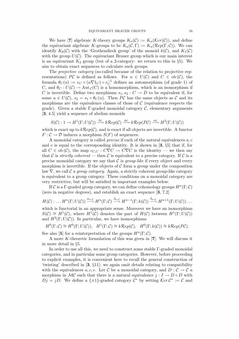
EQUIVARIANT BRAUER GROUPS 59
We have [7] algebraic K-theory groups Kn(C) := Kn(Ker(C)), and definethe equivariant algebraic K-groups to be Kn(C, Γ) := Kn(Rep(Γ, C)). We canidentify K0(C) with the ‘Grothendieck group’ of the monoid k(C), and K1(C)with the group U(C). The equivariant Brauer group which is our main interestis an equivariant K2 group (but of a 2-category: we return to this in §5). Weaim to obtain exact sequences to calculate such groups.
The projective category (so-called because of the relation to projective rep-resentations) PC is defined as follows. For u ∈ U(C) and C ∈ ob (C), theformula θC(u) := eC (u∇1C) e−1
C defines an automorphism (of grade 1) ofC, and θC : U(C) → Aut C(C) is a homomorphism, which is an isomorphism ifC is invertible. Define two morphisms s1, s2 : C → D to be equivalent if, forsome u ∈ U(C), s2 = s1 θC(u). Then PC has the same objects as C and itsmorphisms are the equivalence classes of those of C (equivalence respects thegrade). Given a stable Γ-graded monoidal category C, elementary arguments[3, 4.5] yield a sequence of abelian monoids
S(C) : 1 → H1(Γ; U(C)) φC−→ kRep(C) µC−→ kRep(PC) ωC−→ H2(Γ;U(C))which is exact up to kRep(C), and is exact if all objects are invertible. A functorF : C → D induces a morphism S(F ) of sequences.
A monoidal category is called precise if each of the natural equivalences a, cand e is equal to the corresponding identity. It is shown in [3, §5] that if, forall C ∈ ob (C), the map cC,C : C∇C → C∇C is the identity — we then saythat C is strictly coherent — then C is equivalent to a precise category. If C is aprecise monoidal category we say that C is group-like if every object and everymorphism is invertible. If the objects of C form a group under the compositionlaw ∇, we call C a group category. Again, a strictly coherent group-like categoryis equivalent to a group category. These conditions on a monoidal category arevery restrictive, but will be satisfied in important examples below.
If C is a Γ-graded group category, we can define cohomology groups Hn(Γ; C)(zero in negative degrees), and establish an exact sequence [3, 7.2]
H(C) : . . . Hn(Γ; U(C)) αn,C−→ Hn(Γ; C) βn,C−→ Hn−1(Γ; k(C)) δn,C−→ Hn+1(Γ; U(C)) . . .
which is functorial in an appropriate sense. Moreover we have an isomorphismS(C) ∼= H1(C), where H1(C) denotes the part of H(C) between H1(Γ; U(C))and H2(Γ;U(C)). In particular, we have isomorphisms
H0(Γ; C) ∼= H0(Γ; U(C)), H1(Γ; C) ∼= kRep(C), H0(Γ; k(C)) ∼= kRep(PC).See also [5] for a reinterpretation of the groups Hn(Γ; C).
A more K-theoretic formulation of this was given in [7]. We will discuss itin more detail in §5.
In order to use all this, we need to construct some stable Γ-graded monoidalcategories, and in particular some group categories. However, before proceedingto explicit examples, it is convenient here to recall the general construction of‘twisting’ described in [3, §11]: we again omit details relating to compatibilitywith the equivalences a, c, e. Let C be a monoidal category, and D : C → C amorphism in MC such that there is a natural equivalence j : I → D D withDj = jD. We define a ±1-graded category C∗ by setting Ker C∗ := C and

60 A. FROHLICH AND C.T.C. WALL
letting the morphisms of grade −1 from P to P ′ correspond to C-morphismsfrom DP to P ′. Composition with a morphism P ′ → P ′′ of grade +1 is definedin the natural way; if g : DP ′ → P ′′ defines a morphism in C∗ of grade −1, thecomposite with f : P → P ′ or with f : DP → P ′ is defined by g Df or byg Df jP respectively. This composition is associative since Dj = jD.
If C is Γ-graded, the same construction works to give a Γ × ±1-gradedmonoidal category C∗. Now if w : Γ → ±1 is a homomorphism, with graphΓw ⊂ Γ× ±1, we may restrict to the morphisms whose grades belong to Γw
to obtain a Γw-graded monoidal category, which we say is obtained from C bytwisting.
Similarly, given two triples (C, D, j) and (C′, D′, j′) satisfying the conditions,we can enhance a functor T : C → C′ to T ∗ : C∗ → C′∗ provided we are givena natural transformation h : D′ T → T D such that, for each P ∈ ob C,TjA = hDA D′hA jTA.
2. Construction of categories of modules and algebras
We use ‘ring’ to mean ring with identity element. If Γ is a group, a Γ-ringconsists of a ring E together with an action of Γ by ring automorphisms. If Eand F are Γ-rings, the category EModF of E-F -bimodules is enhanced to a Γ-graded category by defining a morphism M → N of grade γ to be a pair (φ, γ)where φ : M → N is a morphism of additive groups with φ(emf) = eγφ(m)fγ
for all e ∈ E, m ∈ M, f ∈ F . Then Rep(EModF ) is equivalent to the categoryof bimodules with Γ-action. If G is a further Γ-ring there are functors
⊗F : (EModF )×Γ (FModG) → EModG,HomF : (EModop
F )×Γ (GModF ) → GModE
of Γ-graded monoidal categories.Fix a group Γ and a homomorphism w : Γ → ±1. A (Γ, w)-ring consists
of a ring E and an action of Γ on the additive group such that (e1e2)γ = eγ1eγ
2if w(γ) = +1 and eγ
2eγ1 if w(γ) = −1. If w(γ) = −1, a morphism of grade γ
from an E-F -bimodule M to an F -E-bimodule M ′ is a group homomorphismφ such that φ(emf) = fγφ(m)eγ for all e ∈ E, f ∈ F,m ∈ M . The pair (Γ, w)will be fixed throughout §2-§5, and will usually be omitted from the notation.However, we add an affix + to the notation to signify if (Γ, w) is replacedby (Γ, 1). A case of particular interest for the application to quadratic formsis when w is an isomorphism, so the action of Γ on E is given by an involution σ.
From now on we fix a commutative ring R, and consider only R-modules(and algebras) such that the left and right actions of R agree; write ModR (=ZModR) for the category of R-modules. First suppose w trivial. Then ModR isa Γ-graded monoidal category, where — as throughout §2-§4 — we take tensorproduct ⊗ as the operator ∇. Define GenR to be the subcategory of ModR
whose objects are the R-progenerators, i.e. faithful, finitely generated projectiveR-modules, and whose morphisms are the invertible ones of all grades. This isa stable Γ-graded monoidal category.
To deal with the case when w is non-trivial, first observe that taking dualsM∗ = HomR(M, R) of objects and inverse duals f∗ for morphisms gives an

EQUIVARIANT BRAUER GROUPS 61
equivalence ∗ : GenR∼= GenR of Γ-graded monoidal categories so that ∗∗ ∼=
1GenR. We can now use the twisting construction defined earlier. We can
interpret a morphism M → N of grade γ in GenR with w(γ) = −1 is a morphismM∗ → N of grade γ in Gen+
R. There is a natural definition of composition ineach case, leading to a well-defined Γ-graded monoidal category GenR.
The invertible objects of GenR are the invertible R-modules, i.e. rank 1projectives: these form a category CR. The category CR is strictly coherent,hence equivalent to a group category. Write iR : CR → GenR for the inclusionfunctor.
The unit group U(CR) = U(GenR) = U(ModR) is identified with the groupU(R) of units of R, and k(CR) is the Picard group or class group C(R) of R.We inherit actions of Γ on U(R) and C(R). Note that the class cl (M) ∈ C(R)of M ∈ ob (CR) satisfies cl (M∗) = cl (M)−1 and for u ∈ U(GenR), u∗ = u−1.The induced action of Γ on both C(R) and U(R) is thus obtained from thecorresponding action for C+
R by tensoring by w: care is needed with signs in allcases when w is not trivial.
Since morphisms in GenR of grade γ with w(γ) = −1 correspond to ho-momorphisms M∗ → N , or equivalently to pairings between M∗ and N∗, wemay reformulate the definitions as follows. First define the category EPairF
(where E and F are rings) to have objects triples (M, M ′, µ) with M an E-F -bimodule, M ′ an F -E-bimodule and µ : M ×M ′ → E a pairing that defines anE-E-bimodule map M ⊗F M ′ → E. A morphism (M,M ′, µ) → (N,N ′, ν) ofgrade γ is a triple (φ, φ′, γ) where φ and φ′ are morphisms of grade γ and
if w(γ) = 1, φ : M → N , φ′ : M ′ → N ′,if w(γ) = −1, φ : M → N ′, φ′ : M ′ → N ,
and in both cases ν(φ(m), φ′(m′)) = µ(m, m′)γ . There is a functor⊗F : (EPairF )×Γ (FPairG) → EPairG
of monoidal Γ-graded categories. Given h : Γ → AutEPairF
(M,M ′, µ), defineµσ : M ×M → E by µσ(m1,m2) = µ(m1, hσ(m2)). Then µσ is sesquilinear andreflexive: µσ(m1,m2) = µσ(hσ2(m2), m1); if σ2 = 1, µσ is hermitian.
Now for R commutative define PairR := ZPairR, and let GenPairR de-note the full subcategory of PairR whose objects are triples (M,M ′, µ) with Mand M ′ progenerators and µ non-singular. Then if 〈, 〉 : M ×M∗ → R is thecanonical pairing, the embedding functor M 7→ (M, M∗, 〈, 〉) is an equivalenceof Γ-graded monoidal categories from GenR onto GenPairR. We may thus workwith the latter when this is more convenient.
We now define the category AlgR. The objects are associative R-algebraswith identity and if w = 1, a morphism (h, γ) : A → B of grade γ is given bya ring homomorphism h which is a morphism of grade γ in ModR. Taking op-posite algebras defines an equivalence op : AlgR
∼= AlgR of Γ-graded monoidalcategories, so that op op ∼= 1. We may thus again apply the twisting construc-tion. Thus a morphism (h, γ) : A → B of grade γ with w(γ) = −1 is given by aring homomorphism of Aop to B (equivalently, anti-homomorphism h : A → B,i.e. satisfies h(xy) = h(y)h(x)), which is a morphism of grade γ in ModR.

62 A. FROHLICH AND C.T.C. WALL
We pick out the subcategory AzR of AlgR whose objects are the Azumaya(central separable) algebras and whose morphisms are the invertible ones only.Both AlgR and AzR are stable Γ-graded monoidal categories.
Write Lin R : AlgR →ModR for the forgetful functor from an algebra to theunderlying module. If w is trivial, this induces functors Lin R : AlgR →ModR
and Lin R : AzR → GenR of Γ-graded monoidal categories. To extend to thecase when w is non-trivial we require a natural equivalence h : (Lin RA)∗ →Lin R(Aop). For this we use the reduced trace τA : A → R, which is defined forAzumaya algebras and has the properties:
(i) the pairing TA : A × A → R given by TA(a1, a2) = τA(a1a2) is non-singular,
(ii) we have τA(a2a1) = τA(a1a2),(iii) τAop(aop) = τA(a),(iv) if f : A → B is a Γ-ring isomorphism of grade γ, τB(f(a)) = τA(a)γ ,(v) τA⊕B = τA ⊕ τB.
Here (i) shows that the map A → A∗ induced by TA has an inverse, which wecan take as h, (iv) yields the commutative diagram required for compatibility;(ii) and (iii) imply compatibility with the equivalences ‘j’, and (v) with sums.
More directly, we can define Lin R : AzR → GenPairR by Lin R(A) :=(A,A, τA), and check that this defines a functor of Γ-graded monoidal categories,and hence induces a morphism from AzR to GenR.
Taking the endomorphism ring defines a morphism in Γ −MC in the op-posite direction, End R : GenR → AzR. This is clear if w is trivial, and there isan equivalence End R ∗ ∼= op End R of functors of Γ-graded monoidal cate-gories, which allows us to extend to the twisted case. There is now a Γ−MC-equivalence 1AzR
⊗R op ∼= End R Lin R induced by the standard isomorphismjA : A ⊗R Aop ∼= End R(A) given by jA(a ⊗ bop)(c) = acb. Thus the functorEnd R is cofinal.
If (X, h) is an object of Rep(Γ,GenR), so that h : Γ → Aut GenR(X), then
Rep(End R)(X, h) is the object of Rep(Γ,AzR) given by the algebra End R(X),where γ acts by conjugation with the semi-linear automorphism or anti-auto-morphism h(γ) according as w(γ) = 1 or −1. The fibre of the functor End isdescribed by
Lemma 2.1. (i) Let M, N ∈ ob (GenR). Then End R(M) ∼= End R(N) ifand only if, for some P ∈ ob (CR), M ∼= N ⊗R P .
(ii) Let (f, γ), (g, γ) be morphisms in GenR. Then End R(f, γ) = End R(g, γ)if and only if, for some u ∈ C(R), (f, γ) = (u, 1) (g, γ).
(iii) The functor End R : GenR → AzR factors as
GenRPR−→ PGenR
PEndR−→ AzR.
Taking inner automorphisms gives a homomorphism A× → Aut (A) of themultiplicative group A× of invertible elements of A, whose image Inn (A) con-sists of the inner automorphisms. We define new stable Γ-graded monoidalcategories QAlgR and QAzR whose objects are those of AlgR or AzR respec-tively, but morphisms are equivalence classes of morphisms under the relation
f ∼ g : if f = g a for some a ∈ A×
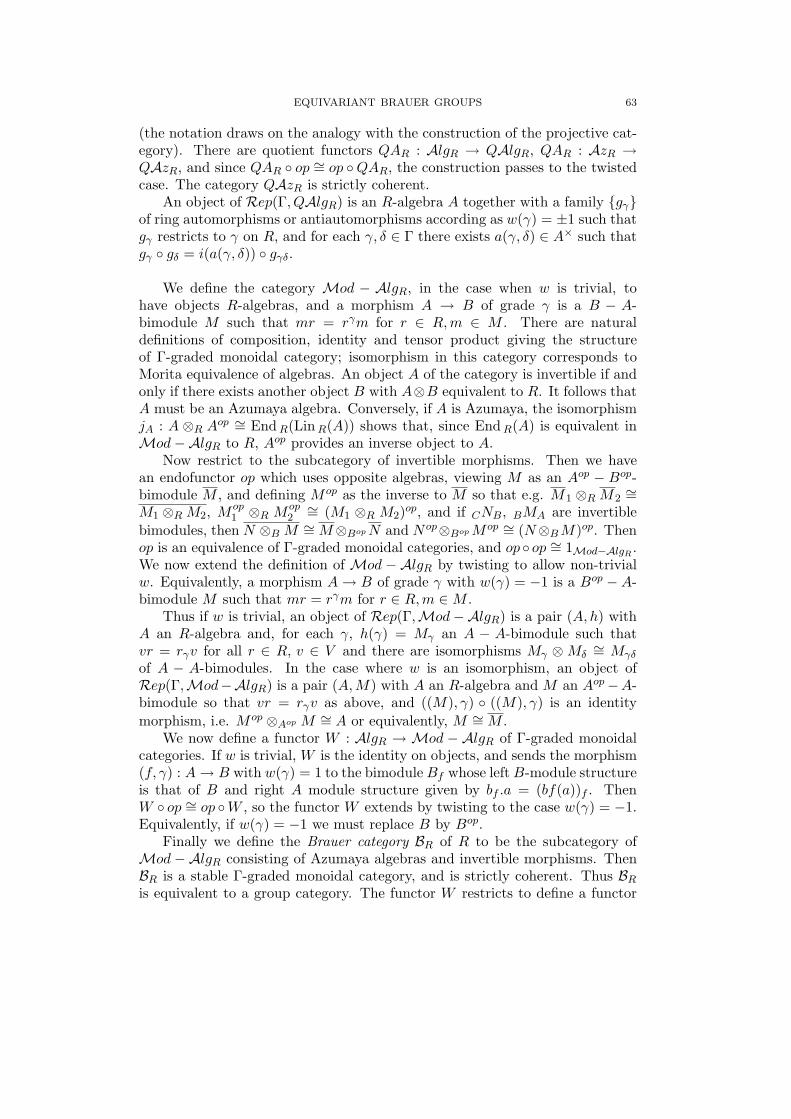
EQUIVARIANT BRAUER GROUPS 63
(the notation draws on the analogy with the construction of the projective cat-egory). There are quotient functors QAR : AlgR → QAlgR, QAR : AzR →QAzR, and since QAR op ∼= op QAR, the construction passes to the twistedcase. The category QAzR is strictly coherent.
An object of Rep(Γ, QAlgR) is an R-algebra A together with a family gγof ring automorphisms or antiautomorphisms according as w(γ) = ±1 such thatgγ restricts to γ on R, and for each γ, δ ∈ Γ there exists a(γ, δ) ∈ A× such thatgγ gδ = i(a(γ, δ)) gγδ.
We define the category Mod − AlgR, in the case when w is trivial, tohave objects R-algebras, and a morphism A → B of grade γ is a B − A-bimodule M such that mr = rγm for r ∈ R, m ∈ M . There are naturaldefinitions of composition, identity and tensor product giving the structureof Γ-graded monoidal category; isomorphism in this category corresponds toMorita equivalence of algebras. An object A of the category is invertible if andonly if there exists another object B with A⊗B equivalent to R. It follows thatA must be an Azumaya algebra. Conversely, if A is Azumaya, the isomorphismjA : A ⊗R Aop ∼= End R(Lin R(A)) shows that, since End R(A) is equivalent inMod−AlgR to R, Aop provides an inverse object to A.
Now restrict to the subcategory of invertible morphisms. Then we havean endofunctor op which uses opposite algebras, viewing M as an Aop − Bop-bimodule M , and defining Mop as the inverse to M so that e.g. M1 ⊗R M2
∼=M1 ⊗R M2, Mop
1 ⊗R Mop2∼= (M1 ⊗R M2)op, and if CNB, BMA are invertible
bimodules, then N ⊗B M ∼= M⊗Bop N and Nop⊗Bop Mop ∼= (N⊗B M)op. Thenop is an equivalence of Γ-graded monoidal categories, and op op ∼= 1Mod−AlgR
.We now extend the definition of Mod − AlgR by twisting to allow non-trivialw. Equivalently, a morphism A → B of grade γ with w(γ) = −1 is a Bop −A-bimodule M such that mr = rγm for r ∈ R, m ∈ M .
Thus if w is trivial, an object of Rep(Γ,Mod−AlgR) is a pair (A, h) withA an R-algebra and, for each γ, h(γ) = Mγ an A − A-bimodule such thatvr = rγv for all r ∈ R, v ∈ V and there are isomorphisms Mγ ⊗ Mδ
∼= Mγδ
of A − A-bimodules. In the case where w is an isomorphism, an object ofRep(Γ,Mod−AlgR) is a pair (A,M) with A an R-algebra and M an Aop−A-bimodule so that vr = rγv as above, and ((M), γ) ((M), γ) is an identitymorphism, i.e. Mop ⊗Aop M ∼= A or equivalently, M ∼= M .
We now define a functor W : AlgR → Mod − AlgR of Γ-graded monoidalcategories. If w is trivial, W is the identity on objects, and sends the morphism(f, γ) : A → B with w(γ) = 1 to the bimodule Bf whose left B-module structureis that of B and right A module structure given by bf .a = (bf(a))f . ThenW op ∼= op W , so the functor W extends by twisting to the case w(γ) = −1.Equivalently, if w(γ) = −1 we must replace B by Bop.
Finally we define the Brauer category BR of R to be the subcategory ofMod−AlgR consisting of Azumaya algebras and invertible morphisms. ThenBR is a stable Γ-graded monoidal category, and is strictly coherent. Thus BR
is equivalent to a group category. The functor W restricts to define a functor

64 A. FROHLICH AND C.T.C. WALL
W : AzR → BR, and this factors through QAR : AzR → QAzR to defineW ′ : QAzR → BR.
3. Exact sequences of k groups and monoids
We now introduce notations for the monoids k of the categories Gen, C,Azand B, and their projective and equivariant versions (the categories Mod,Algand Mod−Alg were merely used in the constructions). Set
Gen(R) := k(GenR) Az(R) := k(AzR)Gen(R, Γ) := k(Rep(Γ,GenR)) Az(R, Γ) := k(Rep(Γ,AzR))
PGen(R, Γ) := k(Rep(Γ, PGenR)) QAz(R, Γ) := k(Rep(Γ, QAzR))C(R) := k(CR) B(R) := k(BR)
C(R, Γ) := k(Rep(Γ, CR)) RB(R, Γ) := k(Rep(Γ,BR))
Then also k(PGenR) = Gen(R) and k(QAzR) = Az(R); and the equivariantclass group C(R, Γ) is the maximal subgroup of the monoid Gen(R, Γ). Wehave various maps induced by the functors
C(R) iR−→ Gen(R) End R−→ Az(R) WR−→ B(R);↓PR
PEndR↓QAR
W ′R
PGenR QAzR
we denote the induced maps of k groups by the same letters; for the maps ofequivariant k groups we add Γ to the subscript. However, the notations formaps to versions of B(R) will be defined ad hoc.
The unit groups of the categories are trivial for PGenR,AzR and QAzR; wemay identify
U(GenR) = U(CR) = U(R), U(BR) ∼= C(R).
We need more care in defining the equivariant versions of the Brauer group.First we define the equivariant Brauer category B(R, Γ). Its objects are those ofRep(Γ,AzR), which are R−Γ-algebras A with groups f(Γ) of (anti)automorph-isms. If w is trivial, a morphism (A, f) → (B, g) is an isomorphism class of pairs(M,h) where M = AMB is an invertible bimodule and h a homomorphism ofΓ to the automorphism group of the additive group M such that hγ(amb) =fγ(a)hγ(m)gγ(b) for all a ∈ A, b ∈ B and m ∈ M .
Here we cannot use the twisting construction since we are not defining agraded category. If w is non-trivial, then to define morphisms A → B westart with the category Rep(Γ, APairB) and consider isomorphism classes ofquintuplets (M, M ′, φ, h, h′) with bimodules AMB, BM ′
A, a non-singular pairingφ : M × M ′ → A over B with φ(hγm,h′γm′) = fγ(φ(m,m′)) and hγ(amb) =gγ(b)hγ(m)fγ(a) for all a, b, m. After some (pages of) checking, we obtain
Proposition 3.1. The category B(R, Γ) is a strictly coherent group-likecategory. The functor WR induces a functor WR,Γ : Rep(Γ,AzR) → B(R, Γ) ofmonoidal categories such that the sequence
Gen(R, Γ)EndR,Γ−→ Az(R, Γ)
WR,Γ−→ k(B(R, Γ))
is exact. Moreover, U(B(R, Γ)) ∼= C(R, Γ).

EQUIVARIANT BRAUER GROUPS 65
Define
B(R, Γ) := k(B(R, Γ))) ∼= CokerEndR,Γ : Gen(R, Γ) → Az(R, Γ).
Then B(R, Γ) is a group, the equivariant Brauer group. Here the cokernel is thegroup of Brauer equivalence classes of (R, Γ)-Azumaya algebras, k(B(R, Γ)) isthe group of Morita equivalence classes, so the isomorphism expresses the factthat equivariant Brauer equivalence is the same as equivariant Morita equiva-lence. Recall that if w is an isomorphism, an equivariant Morita equivalenceinduces isomorphisms of categories of quadratic forms. Thus B(R, Γ) is thegroup identified in the introduction as of particular importance.
If M ∈ ob(GenR) represents a class in H0(Γ;Gen(R)), there exists a sectionh to Aut Gen(R)(M) → Γ. Define hγ := End(hγ). Since hγhδh
−1γδ has grade
1, hγhδh−1γδ is an inner automorphism of EndR(M), so (EndR(M), h) defines
an object of Rep(Γ, QAzR). This object depends only on M and is denotedQEnd(M). This construction induces a homomorphism
QEndR,Γ : H0(Γ; Gen(R)) → QAz(R, Γ).We denote the cokernel — which is a group — by QB(R, Γ), and thus obtaina commutative diagram, whose maps we denote as follows
Gen(R, Γ)EndR,Γ−→ Az(R, Γ)
WR,Γ−→ B(R, Γ)↓TGen
↓QAR,Γ↓QBR,Γ
H0(Γ;Gen(R))QEndR,Γ−→ QAz(R, Γ)
QWR,Γ−→ QB(R, Γ)
Since kRepW ′R : QAz(R, Γ) → RB(R, Γ) vanishes on the image of H0(Γ;
Gen(R)), we have an induced homomorphism θ : QB(R, Γ) → RB(R, Γ).Forgetting the group Γ induces a homomorphism QB(R, Γ) → B(R) whose
image is contained in the invariant subgroup H0(Γ; B(R)). We write Az0(R, Γ),QAz0(R, Γ), B0(R, Γ) and QB0(R, Γ) for the kernels of the respective inducedmaps to B(R). We also add a suffix 0 to denote the restrictions of various maps,e.g. PEndR,Γ,0 : PGen(R, Γ) → Az0(R, Γ).
Theorem 3.2. (i) End R induces an exact sequence of Γ-modules
1 → C(R) iR−→ Gen(R) End R−→ Az(R) WR−→ B(R) → 1.
(ii) The following diagram commutes and the top two rows are exact.
1→ C(R, Γ)iR,Γ−→ Gen(R, Γ)
EndR,Γ−→ Az(R, Γ)WR,Γ−→ B(R, Γ) →1
↓TC ↓TGen ↓QAR,Γ ↓QBR,Γ
1→H0(Γ; C(R))H0(iR)−→ H0(Γ; Gen(R))
QEndR,Γ−→ QAz(R, Γ)QWR,Γ−→ QB(R, Γ) →1
| ↓ | ↓ ↓ TQAz ↓ TQB
H0(Γ; C(R))H0(iR)−→ H0(Γ; Gen(R))
H0(EndR)−→ H0(Γ; Az(R))H0(WR)−→ H0(Γ; B(R))
Exactness for sequences of monoids is interpreted in accordance with thedefinitions in the appendix to [3]: here, in particular, the functor End R iscofinal.
We also have exact sequences S(C) with C any of CR, GenR and BR and,more importantly, H(C) with C either of CR and BR. Explicitly, these are

66 A. FROHLICH AND C.T.C. WALL
H(CR) . . .Hn(Γ;U(R))αn,C−→ Hn(Γ; CR)
βn,C−→ Hn−1(Γ;C(R))δn,C−→ Hn+1(Γ; U(R)) . . .
H(BR) . . .Hn(Γ;C(R))αn,B−→ Hn(Γ;BR)
βn,B−→ Hn−1(Γ;B(R))δn,B−→ Hn+1(Γ;C(R)) . . .
Theorem 3.3. There is a commutative diagram with exact rows and injec-tive columns
1 → QB0(R, Γ) −→ QB(R, Γ) −→ H0(Γ; B(R))↓ ξ ↓ θ |↓
1 → H1(Γ; C(R))α1,B−→ H1(Γ;BR)
β1,B−→ H0(Γ; B(R))
To prove this, we first establish that an algebra representing an element ofKer θ is in ImQEndR,Γ, and then apply Theorem 3.2 to see that θ is injective.Now the upper row is trivially exact, and the lower is part of H(BR). Sincethe right hand square clearly commutes, there is an induced map ξ, which isinjective since θ is.
We now give two direct constructions of maps to H3(Γ; U(R)). If G isa group, with centre Z(G) and group Out (G) := Aut (G)/Inn (G) of outerautomorphisms, then to any homomorphism h : Γ → Out (G) is associated acohomology class c(h) ∈ H3(Γ;Z(G)), the obstruction to the existence of agroup extension of G by Γ inducing h.
For A an R-algebra, write Aut +(A) for its group of automorphisms and anti-automorphisms; recall that A× denotes the multiplicative group of invertibleelements. Define
κA : Aut +(A) → Aut (A×)by κA(t)(u) = t(u) if t is an automorphism, and t(u)−1 if t is an anti-auto-morphism. This induces a homomorphism
κA : Aut +(A)/Inn (A) → Out (A×).If (A, f) is an object of Rep(Γ,AzR), f is a homomorphism of Γ to the
quotient Aut +(A)/Inn (A), hence we have a homomorphismκA f : Γ → Out (A×)
and hence — since we can identify Z(A×) = U(R) — a cohomology classρ(A, f) := c(κA f) ∈ H3(Γ; U(R)).
Next let (A, (M)) ∈ obRep(Γ,BR). For each γ ∈ Γ with w(γ) = 1, Mγ
is an invertible A − A-bimodule of grade γ, and if w(γ) = w(δ) = 1 we maychoose isomorphisms fγ,δ : Mγ ⊗A Mδ
∼= Mγδ. If however w(γ) = 1 butw(δ) = −1, Mδ is an Aop−A-bimodule, and we get instead an isomorphism fγ,δ :Mop
γ ⊗Aop Mδ∼= Mγδ. Given 3 elements γ1, γ2, γ3 ∈ Γ we get two isomorphisms
(of grade 1)a(γ1, γ2, γ3), b(γ1, γ2, γ3) : M ′
γ1⊗M ′
γ2⊗M ′
γ3−→ M ′
γ1γ2γ3,
where M ′γ denotes Mγ or Mop
γ and the tensor products are over A or Aop
according to the values w(γi).Set u(γ1, γ2, γ3) := b(γ1, γ2, γ3) · a(γ1, γ2, γ3)−1. This is a grade 1 automor-
phism of an invertible module, so can be identified with an element of U(R).Further calculations show that u defines a 3-cocycle of Γ with values in U(R),and that varying the choice of the isomorphisms f(γ, δ) by multiplying by a fam-ily v(γ, δ) of elements of U(R) has the effect of multiplying u by the coboundaryof v. We thus obtain a well defined cohomology class χ(A, (M)) ∈ H3(Γ; U(R)).

EQUIVARIANT BRAUER GROUPS 67
Theorem 3.4. The above constructions define(i) a map ρ : QB(R, Γ) → H3(Γ; U(R)) which is zero on the image of B(R, Γ),(ii) a homomorphism χ : RB(R, Γ) → H3(Γ;U(R)), such that(iii) we have ρ = χ θ : QB(R, Γ) → RB(R, Γ) → H3(Γ;U(R)),(iv) we have δCR
= χ αBR: H1(Γ;C(R)) → RB(R, Γ) → H3(Γ; U(R))
up to eventual signs!For A an Azumaya R-algebra, write AM∗
R for the category of A − R-bimodules where R acts the same way on both sides; note that tensor productgives a functor ⊗R :A M∗
R × CR →A M∗R.
Lemma 3.5. (i)Let Ai ∈ ob (AzR), Mi ∈ ob (AiM∗R), Pi ∈ ob (CR) for
i = 1, 2, and let α : A1 → A2 be a morphism in AzR and f : M1 → M2,g : M1⊗RP1 → M2⊗RP2 be isomorphisms of additive groups over the morphismα. Then there is a unique R-module isomorphism c : P1 → P2 with g = f ⊗R c.
(ii) A corresponding conclusion holds if Γ acts on R and α is a morphismof grade γ, also if w(γ) = −1.
Let (A, t) ∈ ob (Rep(Γ,AzR)), so t : Γ → AutAzR(A). Suppose we have an
invertible A − R-bimodule M . Then if w(γ) = 1 we have P (γ) ∈ ob (CR) anda group isomorphism fγ : M → M ⊗R P (γ) such that fγ(am) = tγ(a)fγ(m)for all a ∈ A,m ∈ M . If w(γ) = −1 we have P (γ) ∈ ob (CR) and a groupisomorphism fγ : M → P (γ)∗ ⊗R M∗ such that fγ(am) = fγ(m)tγ(a) for alla ∈ A,m ∈ M . From Lemma 3.5 we have unique additive isomorphisms
c(γ1, γ2) : p(γ2) →
P (γ1)∗ ⊗R P (γ1γ2) if w(γ1) = 1(P (γ1)∗ ⊗R P (γ1γ2))∗ if w(γ1) = −1
such that fγ1γ2 · f−1γ2
= [fγ1 , c(γ1, γ2)]. The elements c(γ1, γ2) define a cocyclewhose class in H2(Γ; CR) is independent of the choices of the Pγ and fγ . Theresulting map ψ′ : Az0(R, Γ) → H2(Γ; CR) is a monoid homomorphism inducingan injective homomorphism ψ : B0(R, Γ) → H2(Γ; CR).
Denote by τ the composite map
PGen(R, Γ)PEndR,Γ,0−→ Az0(R, Γ)
WR,Γ,0−→ B0(R, Γ).
Theorem 3.6. The following diagram is commutative (up to signs) and theupper row is exact at B0(R, Γ).
PC(R, Γ)PiR,Γ−→ PGen(R, Γ) τ−→ B0(R, Γ)
QBR,Γ,0−→ QB0(R, Γ)↓o ↓ ωGen ↓ ψ ↓ ξ
H0(Γ;C(R))δ1,C−→ H2(Γ; U(R)
α2,C−→ H2(Γ : CR)β2,C−→ H1(Γ;C(R))
4. Finite groups
We will now assume Γ to be finite. With this restriction we can strengthenthe foregoing results.
Theorem 4.1. Let Γ be finite. Then(i) the map ωGen : PGen(R, Γ) → H2(Γ : U(R)) is surjective;(ii) the following maps are isomorphisms:
θ : QB(R, Γ) → k(Rep(Γ,BR)),
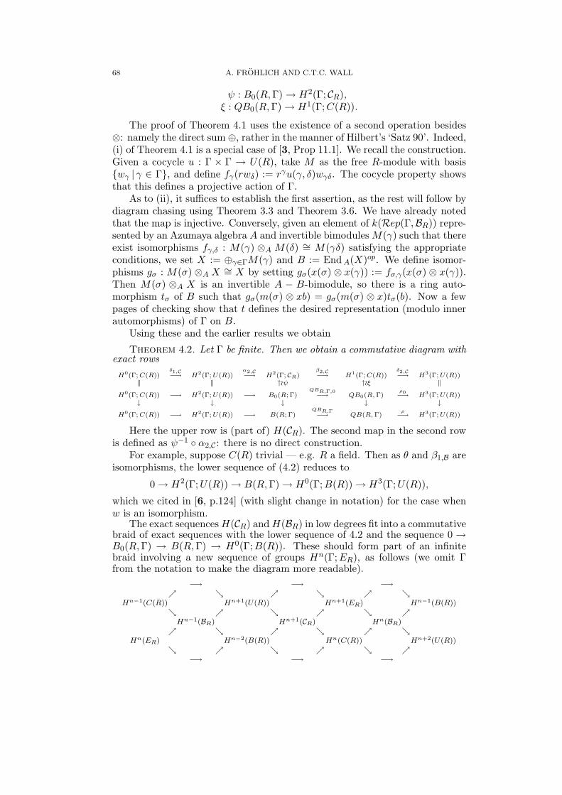
68 A. FROHLICH AND C.T.C. WALL
ψ : B0(R, Γ) → H2(Γ; CR),ξ : QB0(R, Γ) → H1(Γ; C(R)).
The proof of Theorem 4.1 uses the existence of a second operation besides⊗: namely the direct sum ⊕, rather in the manner of Hilbert’s ‘Satz 90’. Indeed,(i) of Theorem 4.1 is a special case of [3, Prop 11.1]. We recall the construction.Given a cocycle u : Γ × Γ → U(R), take M as the free R-module with basiswγ | γ ∈ Γ, and define fγ(rwδ) := rγu(γ, δ)wγδ. The cocycle property showsthat this defines a projective action of Γ.
As to (ii), it suffices to establish the first assertion, as the rest will follow bydiagram chasing using Theorem 3.3 and Theorem 3.6. We have already notedthat the map is injective. Conversely, given an element of k(Rep(Γ,BR)) repre-sented by an Azumaya algebra A and invertible bimodules M(γ) such that thereexist isomorphisms fγ,δ : M(γ) ⊗A M(δ) ∼= M(γδ) satisfying the appropriateconditions, we set X := ⊕γ∈ΓM(γ) and B := End A(X)op. We define isomor-phisms gσ : M(σ) ⊗A X ∼= X by setting gσ(x(σ) ⊗ x(γ)) := fσ,γ(x(σ) ⊗ x(γ)).Then M(σ) ⊗A X is an invertible A − B-bimodule, so there is a ring auto-morphism tσ of B such that gσ(m(σ) ⊗ xb) = gσ(m(σ) ⊗ x)tσ(b). Now a fewpages of checking show that t defines the desired representation (modulo innerautomorphisms) of Γ on B.
Using these and the earlier results we obtain
Theorem 4.2. Let Γ be finite. Then we obtain a commutative diagram withexact rows
H0(Γ; C(R))δ1,C−→ H2(Γ; U(R))
α2,C−→ H2(Γ; CR)β2,C−→ H1(Γ; C(R))
δ2,C−→ H3(Γ; U(R))‖ ‖ ↑oψ ↑oξ ‖
H0(Γ; C(R)) −→ H2(Γ; U(R)) −→ B0(R; Γ)QBR,Γ,0−→ QB0(R, Γ)
ρ0−→ H3(Γ; U(R))↓ ↓ ↓ ↓ ↓
H0(Γ; C(R)) −→ H2(Γ; U(R)) −→ B(R; Γ)QBR,Γ−→ QB(R, Γ)
ρ−→ H3(Γ; U(R))
Here the upper row is (part of) H(CR). The second map in the second rowis defined as ψ−1 α2,C : there is no direct construction.
For example, suppose C(R) trivial — e.g. R a field. Then as θ and β1,B areisomorphisms, the lower sequence of (4.2) reduces to
0 → H2(Γ;U(R)) → B(R, Γ) → H0(Γ; B(R)) → H3(Γ; U(R)),
which we cited in [6, p.124] (with slight change in notation) for the case whenw is an isomorphism.
The exact sequences H(CR) and H(BR) in low degrees fit into a commutativebraid of exact sequences with the lower sequence of 4.2 and the sequence 0 →B0(R, Γ) → B(R, Γ) → H0(Γ;B(R)). These should form part of an infinitebraid involving a new sequence of groups Hn(Γ; ER), as follows (we omit Γfrom the notation to make the diagram more readable).
−→ −→ −→
Hn−1(C(R)) Hn+1(U(R)) Hn+1(ER) Hn−1(B(R))
Hn−1(BR) Hn+1(CR) Hn(BR)
Hn(ER) Hn−2(B(R)) Hn(C(R)) Hn+2(U(R))
−→ −→ −→

EQUIVARIANT BRAUER GROUPS 69
Here it follows from the diagram that we need to identify H0(ER) ∼= H0(CR) ∼=H0(U(R)) and H1(ER) ∼= H1(CR), while H2(ER) = B(R, Γ) is our centralobject of interest. We turn to the methods of [7] to seek a direct approach tothis conjecture.
5. An abstract approach
In this section we recall and slightly amplify some results from [7]. First,suppose C is a Γ-graded group like category. Define a simplicial space BCwhose 0-simplices are objects of C, 1-simplices are morphisms (of all grades),2-simplices are commutative triangles of morphisms, and higher simplices arefilled in when possible. Then BC fibres over BΓ and the fibre BKer C is aninfinite loop space with K0(C) := π0(BC) = k(C); K1(C) := π1(BC) = U(C),and vanishing higher groups. Further [7, Theorem] there is a spectral sequencewith Ep,q
2 = Hp(Γ; K−q(C)) and abutment K−n(C, Γ) (we have changed somesigns to conform with standard notation for a cohomology spectral sequence).Since only two groups Kq(C) are non-vanishing, the spectral sequence reducesto an exact sequence, which is naturally identified with H(C).
For the present purpose we need a slightly more elaborate construction.Define a simplicial space E as follows. The 0-simplices are the Azumaya R-algebras Ai. The 1-simplices are the invertible bimodules iMj = AiMAj (of allgrades). The 2-simplices are the bimodule isomorphisms fi,j,k : iMj⊗Aj jMk →iMk. The 3-simplices are the commutative diagrams
∆ijkl :iMj ⊗ jMk ⊗ kMl
1⊗fj,k,l−→ iMj ⊗ jMl
↓fi,j,k⊗1 ↓fi,j,l
iMk ⊗ kMlfi,k,l−→ iMl
and the n-simplices for n > 3 are the maps of the 3-skeleton of the standardn-simplex to the partial complex just constructed. There is a map to theclassifying complex BΓ which takes each 1-simplex to its grade.
We claim that E is a Kan complex, and hence that E → BΓ is a Kanfibration. We need to show, for each n, that any map into E of the complexΛn−1 (obtained from the standard n-simplex ∆n by deleting the interiors of then-simplex and of one of its (n− 1)-dimensional faces) extends to a map of ∆n.Since Λn−1 contains the (n− 2)-skeleton of ∆n, this is trivial for n ≥ 5.
For n = 1 the extension is possible since the Γ-grading on BR is stable -given A there exist invertible bimodules of all grades.
For n = 2 if the missing face is the third, we complete the map of Λ1 definedby the modules iMj and jMk by the isomorphism iMj ⊗Aj jMk → iMk. If themissing face is different, the argument is essentially the same, since all thebimodules are invertible, and we may use their inverses.
For n = 3 a map of Λ2 gives (perhaps after tensoring with some identitymaps) the isomorphisms on 3 edges of the desired commutative diagram, andwe may then complete the diagram uniquely.
Finally for n = 4 we are given 4 commutative diagrams and need to establishcommutativity of a fifth. This follows from the following diagram, where wetake the subscripts as 0, 1, 2, 3, 4 and omit the symbol M for brevity:

70 A. FROHLICH AND C.T.C. WALL
(01)⊗ (12)⊗ (23)⊗ (34) −→ −→ −→ (01)⊗ (12)⊗ (24)↓ ↓
(02)⊗ (23)⊗ (34) −→ (02)⊗ (24)↓ ↓ ↓ ↓
(03)⊗ (34) −→ (04)↓ ↓
(01)⊗ (13)⊗ (34) −→ −→ −→ (01)⊗ (14)
Here commutativity of the outer square follows from taking the tensor productof M01 with the simplex ∆1234, of the left square follows from taking the tensorproduct of M34 with the simplex ∆0123, of the centre square from ∆0234, ofthe right square from ∆0124, of the lower square from ∆0134, and of the uppersquare from the identity (f ⊗ 1)(1⊗ g) = (1⊗ g)(f ⊗ 1) where f and g are themorphisms corresponding to the 1-simplices 012 and 234. Since all the mapsare isomorphisms, commutativity of any one square follows from that of therest, as desired.
There is thus again a spectral sequence. If, as seems fairly certain, thefibre is an infinite loop space, the E2 term is determined since we can identifyKq(Ker C) with U(R) if q = 2, C(R) if q = 1, B(R) if q = 0, and 0 otherwise.Unfortunately, the abutment is given only in terms of homotopy groups of thespace of sections, and so is not easily interpreted.
We conjecture that, as in the case first described, there is an algebraicmodel for the spectral sequence, given in terms of some cochain model. Wethen expect that, up to chain homotopy equivalence, the spectral sequence isthat of a filtered complex 0 ⊂ F0 ⊂ F1 ⊂ F2 of free Γ-modules, zero in negativedegrees, such that F0, F1/F0 and F2/F1 give free resolutions of U(R), C(R) andB(R) respectively; and the hypercohomology groups of F1 and F2/F0 give theequivariant cohomology groups of the categories CR and BR. Thus the two ‘new’sequences at the end of §4 would be the exact cohomology sequences belongingto F0 → F2 → F2/F0 and F1 → F2 → F2/F1 respectively.
6. Change of groups
For the case of graded monoidal categories, a rather full discussion of con-structions involving change of groups was given in [3, §9]. We content ourselveshere with a brief summary.
The most general formulation is as follows. For Γ a group, and X a finiteΓ-set, we form the Γ-graded category XΓ whose object set is X and morphismset (x, γ) : x → xγ |x ∈ X, γ ∈ Γ. If C is a Γ-graded monoidal category,H(X) := HomΓ(XΓ, C) can be considered a monoidal category, and H definesa Mackey functor from the category of finite Γ-sets to the homotopy categoryof MC, and hence, composing e.g. with k, to the category of abelian monoids.If C is group-like we may compose with H i(Γ;−) to get a Mackey functor toabelian groups.
It follows, for example, that if Γ has finite order N , then [3, 7.7] N annihi-lates Hn(Γ; C) for n ≥ 2: this result is useful in some applications.
Let C be a Γ-graded group-like monoidal category, and i : ∆ → Γ the inclu-sion of a subgroup. Then there are restriction maps i∗ : H i(Γ; C) → H i(∆; C)
EQUIVARIANT BRAUER GROUPS 71
and, if the subgroup ∆ has finite index, corestriction maps i∗ in the oppositedirection: in particular, i∗ : Rep(Γ, C) → Rep(∆, C) and i∗ : Rep(∆, C) →Rep(Γ, C). Since H is a Mackey functor, these satisfy the standard relations:in fact [1] K0Rep is a Frobenius functor.
If ∆ is a normal subgroup of Γ, then Rep(∆, C) has the natural structureof Γ/∆-graded monoidal category, and [1] Rep(Γ/∆,Rep(∆, C)) ∼= Rep(Γ, C).Presumably if C is a group category there is a spectral sequence with E2-term Hp(Γ/∆; Hq(∆; C)) and abutment Hn(Γ; C); at least we have [3, 9.7] theexpected exact sequence of terms of low degree. This applies to the case C = CR,and in view of the isomorphism ψ gives information about B0(R; Γ) if Γ is finite.
Finally we return to the twisting relation. Let C be a Γ-graded monoidalcategory, and D : C → C a morphism allowing us to extend the grading toΓ × ±1. Suppose given two homomorphisms wi : Γ → ±1 (i = 1, 2) withequaliser ∆: write Γi ⊂ Γ × ±1 for the graph of wi, and ∆ := (∆, w1|∆).Then [3, 10.2] there is a long exact sequence
· · ·H i(Γ1; C) −→ H i(∆; C) −→ H i(Γ2; C) −→ H i+1(Γ1; C) −→ · · ·where the first map is restriction and the second is corestriction. Specialisingto CR, this gives0 → H0(Γ1; U(R)) → H0(∆;U(R)) → H0(Γ2;U(R)) → C(R, Γ1) → C(R, ∆) →
→ C(R, Γ2) → B0(R, Γ1) → B0(R, ∆) → B0(R, Γ2).Perhaps the most interesting case is the simplest, when Γ has order 2, so w1 isan isomorphism and w2 is trivial (or vice-versa), and ∆ is trivial. The exactnessof these sequences may be verified directly.
We may also construct a braid with the exact sequences H(Γ1, C), H(Γ2, C),H(∆, C), and exact cohomology sequences with coefficients U(R) and C(R).
References
[1] A. Frohlich and C.T.C. Wall, Foundations of equivariant algebraic K-theory, Springerlecture notes in Math. 108 (1969) 12–27.
[2] A. Frohlich and C.T.C. Wall, Equivariant Brauer groups in algebraic number theory,Bull. Math. Soc. France Memoire 25 (1971) 91–96.
[3] A. Frohlich and C.T.C. Wall, Graded monoidal categories, Compositio Math. 28 (1974)229–286.
[4] S. MacLane, Natural associativity and commutativity, Rice Univ. Studies 49iv (1963)28-46.
[5] K.-H. Ulbrich, On cohomology of graded group categories, Compositio Math. 63 (1987)409–417.
[6] C.T.C. Wall, On the classification of Hermitian forms II: semisimple rings, Invent. Math.18 (1972) 119-141.
[7] C.T.C. Wall, Equivariant algebraic K-theory, pp 111–118 in New developments in topol-ogy, London Math. Soc. lecture notes 11 (1974).
72 A. FROHLICH AND C.T.C. WALL
Robinson CollegeCambridge CB3 9ANUnited Kingdom
Dept. of Mathematical SciencesLiverpool UniversityLiverpool L69 3BXUnited KingdomE-mail address: [email protected]

Contemporary Mathematics
Isotropy of quadratic forms and field invariants
Detlev W. Hoffmann
Dedicated to the memory of Oleg Izhboldin
Abstract. This paper is intended to give a survey for non-specialists in thealgebraic theory of quadratic forms on the question of isotropy of quadraticforms and how certain answers to this question can be obtained by consideringinvariants of quadratic forms, such as the classical invariants dimension, signeddiscriminant, Clifford invariant, and invariants of fields pertaining to quadraticforms, such as the u-invariant, the Hasse number, the level, the Pythagorasnumber, and the l-invariant. We will interpret these field invariants as thesupremum of the dimensions of certain types of anisotropic quadratic formsdefined over the ground field. Particular emphasis is laid on the question ofwhich values can be realized as invariants of a field, and on methods of howto construct such fields “generically.”
1. Introduction
One of the central questions in the algebraic theory of quadratic forms is thefollowing : When is a given quadratic form ϕ over a field F isotropic, i.e. whendoes the form ϕ represent zero nontrivially ?1
An answer to this question would automatically lead to an answer of anothercentral problem, namely, when are two forms ϕ and ψ of the same dimensionisometric (in which case we write ϕ ∼= ψ), i.e. when does there exist a linearisomorphism t : V → W of the underlying vector spaces V of ϕ and W of ψ suchthat ϕ(v) = ψ(tv) for all v ∈ V ? This can be seen as follows. The diagonal form〈1,−1〉 is called a hyperbolic plane, which we shall also denote by H. A form iscalled hyperbolic if it has a diagonalization of the form 〈1,−1, 1,−1, · · · , 1,−1〉, i.e.if it is isometric to an orthogonal sum of hyperbolic planes, H ⊥ H ⊥ · · · ⊥ H.Now ϕ being isotropic is equivalent to ϕ containing H as a subform.2 If two formsϕ and ψ are of the same dimension, then their isometry is equivalent to ϕ ⊥ −ψ
1991 Mathematics Subject Classification. 11E04, 11E10, 11E25, 11E81, 12D15, 12F20.1Throughout this paper, we only consider fields of characteristic different from 2, and qua-
dratic forms are always assumed to be finite-dimensional and nondegenerate. We will often simplywrite “form” by which we shall refer to quadratic forms in the above sense.
2We say that η is a subform of µ if there exists a form τ such that µ ∼= η ⊥ τ . In thissituation, we write η ⊂ µ for short.
c©0000 (copyright holder)
73
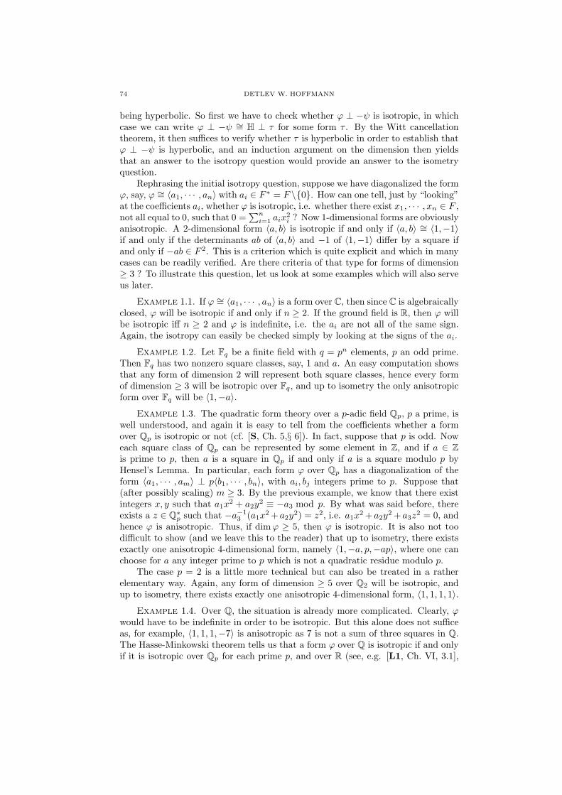
74 DETLEV W. HOFFMANN
being hyperbolic. So first we have to check whether ϕ ⊥ −ψ is isotropic, in whichcase we can write ϕ ⊥ −ψ ∼= H ⊥ τ for some form τ . By the Witt cancellationtheorem, it then suffices to verify whether τ is hyperbolic in order to establish thatϕ ⊥ −ψ is hyperbolic, and an induction argument on the dimension then yieldsthat an answer to the isotropy question would provide an answer to the isometryquestion.
Rephrasing the initial isotropy question, suppose we have diagonalized the formϕ, say, ϕ ∼= 〈a1, · · · , an〉 with ai ∈ F ∗ = F \0. How can one tell, just by “looking”at the coefficients ai, whether ϕ is isotropic, i.e. whether there exist x1, · · · , xn ∈ F ,not all equal to 0, such that 0 =
∑ni=1 aix
2i ? Now 1-dimensional forms are obviously
anisotropic. A 2-dimensional form 〈a, b〉 is isotropic if and only if 〈a, b〉 ∼= 〈1,−1〉if and only if the determinants ab of 〈a, b〉 and −1 of 〈1,−1〉 differ by a square ifand only if −ab ∈ F 2. This is a criterion which is quite explicit and which in manycases can be readily verified. Are there criteria of that type for forms of dimension≥ 3 ? To illustrate this question, let us look at some examples which will also serveus later.
Example 1.1. If ϕ ∼= 〈a1, · · · , an〉 is a form over C, then since C is algebraicallyclosed, ϕ will be isotropic if and only if n ≥ 2. If the ground field is R, then ϕ willbe isotropic iff n ≥ 2 and ϕ is indefinite, i.e. the ai are not all of the same sign.Again, the isotropy can easily be checked simply by looking at the signs of the ai.
Example 1.2. Let Fq be a finite field with q = pn elements, p an odd prime.Then Fq has two nonzero square classes, say, 1 and a. An easy computation showsthat any form of dimension 2 will represent both square classes, hence every formof dimension ≥ 3 will be isotropic over Fq, and up to isometry the only anisotropicform over Fq will be 〈1,−a〉.
Example 1.3. The quadratic form theory over a p-adic field Qp, p a prime, iswell understood, and again it is easy to tell from the coefficients whether a formover Qp is isotropic or not (cf. [S, Ch. 5,§ 6]). In fact, suppose that p is odd. Noweach square class of Qp can be represented by some element in Z, and if a ∈ Zis prime to p, then a is a square in Qp if and only if a is a square modulo p byHensel’s Lemma. In particular, each form ϕ over Qp has a diagonalization of theform 〈a1, · · · , am〉 ⊥ p〈b1, · · · , bn〉, with ai, bj integers prime to p. Suppose that(after possibly scaling) m ≥ 3. By the previous example, we know that there existintegers x, y such that a1x
2 + a2y2 ≡ −a3 mod p. By what was said before, there
exists a z ∈ Q∗p such that −a−13 (a1x
2 +a2y2) = z2, i.e. a1x
2 +a2y2 +a3z
2 = 0, andhence ϕ is anisotropic. Thus, if dim ϕ ≥ 5, then ϕ is isotropic. It is also not toodifficult to show (and we leave this to the reader) that up to isometry, there existsexactly one anisotropic 4-dimensional form, namely 〈1,−a, p,−ap〉, where one canchoose for a any integer prime to p which is not a quadratic residue modulo p.
The case p = 2 is a little more technical but can also be treated in a ratherelementary way. Again, any form of dimension ≥ 5 over Q2 will be isotropic, andup to isometry, there exists exactly one anisotropic 4-dimensional form, 〈1, 1, 1, 1〉.
Example 1.4. Over Q, the situation is already more complicated. Clearly, ϕwould have to be indefinite in order to be isotropic. But this alone does not sufficeas, for example, 〈1, 1, 1,−7〉 is anisotropic as 7 is not a sum of three squares in Q.The Hasse-Minkowski theorem tells us that a form ϕ over Q is isotropic if and onlyif it is isotropic over Qp for each prime p, and over R (see, e.g. [L1, Ch. VI, 3.1],

ISOTROPY OF QUADRATIC FORMS AND FIELD INVARIANTS 75
[S, Ch. 5, Theorem 7.2]). In particular, by the previous example, each indefiniteform of dimension ≥ 5 over Q will be isotropic.
Using the previous example, we see that 〈1, 1, 1,−7〉 is isotropic over each Qp,p 6= 2, and over R. However, it is anisotropic over Q2 since 〈1, 1, 1,−7〉 ∼= 〈1, 1, 1, 1〉over Q2.
Before we consider rational function fields in one variable over the above fields,we shall mention a little lemma which we shall use quite often regarding forms overpurely transcendental extensions.
Lemma 1.5. (i) Let ϕ and ψ be forms over F and let K = F (T ), the rationalfunction field in one variable, or K = F ((T )), the power series field in one variableover F . Then ϕ ⊥ Tψ is anisotropic over K if and only if ϕ and ψ are anisotropicover F . In particular, anisotropic forms stay anisotropic over purely transcendentalextensions.
(ii) If γ is a form over K = F ((T )), then there exist forms ϕ and ψ over F suchthat γ ∼= ϕ ⊥ Tψ.
The first part can easily be proved by a degree argument. As for the secondpart, one may assume that γ is diagonalized and then use the fact that to eachx ∈ K∗ there exists a y ∈ F ∗ such that either x ≡ y mod K∗2 or x ≡ yT mod K∗2.We leave the details to the reader.
Example 1.6. C is algebraically closed and therefore it is a so-called C0 field.3
Hence, C(T ) is a C1-field (cf. [S, Ch. 2, Th. 15.2]), which implies that every formof dimension ≥ 3 over C(T ) will be isotropic.
Example 1.7. As for R(T ), the situation is more complicated. On R, thereexists exactly one ordering.4 On R(T ), there are many orderings which can bedescribed explicitly (cf. [KS, Kap. II, § 9]). Let XR(T ) be the space of orderings.An obvious necessary condition for a form ϕ to be isotropic over R(T ) is that ϕbe totally indefinite, i.e. if ϕ ∼= 〈a1, · · · , an〉 then for each ordering P ∈ XR(T )
there exist ai and aj depending on P such that ai <P 0 <P aj . Using the explicitdescription of the orderings, the indefiniteness can in principal be checked using thecoefficients of a diagonalization. It can also be shown that totally indefinite formsof dimension ≥ 3 over R(T ) are always isotropic, a result essentially due to Witt[Wi1].
Example 1.8. Now consider the rational function field Q(T ) in one variableX over the rationals. Again, the field is formally real, i.e. there exist orderings onQ(T ), and a necessary condition for a form ϕ to be isotropic is that ϕ be indefinitewith respect to all orderings P in the space of orderings XQ(T ). However, thisknowledge alone won’t help us much as there exist anisotropic totally indefiniteforms of any dimension ≥ 2 over Q(T ). This can be seen as follows. Consider theanisotropic forms 〈1,−2〉 and σn = n × 〈1〉 = 〈1, · · · , 1︸ ︷︷ ︸
n
〉 over Q. Then 2 is a sum
of squares and hence 2 ∈ P for all P ∈ XQ(T ). In particular, 〈1,−2〉 ⊥ Tσn is
3A field F is called a Ci-field if every homogeneous polynomial over F of degree d in at leastdi + 1 variables has a nontrivial zero.
4An ordering on a field F is a subset P ⊂ F such that P + P ⊂ P , P · P ⊂ P , P ∪−P = F ,P ∩−P = 0. It induces the order relation “≥P ” defined by x ≥p y if and only if x− y ∈ P . Cf.
[S, Ch. 3, § 1].
76 DETLEV W. HOFFMANN
totally indefinite and anisotropic over Q(T ) for all n (the anisotropy follows fromLemma 1.5).
One can justifiably say that we have no systematic method whatsoever to decidewhether an arbitrarily given form over Q(T ) is isotropic or not. One could say thatwith respect to many questions regarding quadratic forms, the field Q(T ) is of acomplexity which is beyond our current reach.
Example 1.9. Although the quadratic form theory over Qp is in a certain senseeasier to handle than that over Q, not much was known about the isotropy of formsover Qp(T ) until recently, when it was shown in [HVG2] that all ϕ of dimension> 22 over Qp(T ), p 6= 2, are isotropic. Later on, this was improved by Parimalaand Suresh [PS], who proved that in fact all forms of dimension > 10 over Qp(T ),p 6= 2, are isotropic. The case p = 2 is still open.
As we have already remarked above, there does exist an anisotropic 4-dimen-sional form ϕp over Qp for all primes p. This will yield the anisotropic 8-dimensionalform ϕp ⊥ Tϕp over Qp(T ). It is conjectured that all forms of dimension > 8 overQp(T ) are isotropic.
All these examples give us already a glimpse of the difficulties which we en-counter concerning the isotropy of forms. When dealing with forms over a particularfield, one normally develops and uses a set of tools and methods to which quadraticforms over the field in question are amenable. These methods often come from num-ber theory, algebraic and real algebraic geometry. For general fields, one approachto derive information on the isotropy of forms is to consider certain invariants ofquadratic forms resp. of the underlying field and how these invariants influence theisotropy behaviour.
In section 2, we shall introduce quadratic form invariants and show how theycan be used to classify forms resp. to tell us something about isotropy of forms.First, in section 2.1, we introduce the classical invariants dimension, determinantresp. signed discriminant, Clifford invariant and total signature. After saying alittle about the Witt ring of a field and how these invariants can be interpreted asinvariants of elements in this ring in section 2.2, we show in section 2.3 how theclassical invariants lead us inevitably to higher cohomological invariants and theMilnor conjecture (see also Pfister’s survey article [P5]). In section 2.4, we explainhow these invariants lead to classification results on quadratic forms and mentionhow the invariants of a form ϕ (resp. the “place” where the form finds itself in theWitt ring) can provide information on isotropy.
In section 3, we introduce field invariants which can be defined as the supremaof the dimensions of certain types of anisotropic forms over a field F and whichtherefore, once these invariants have been determined for a certain field F , yieldinformation on the (an)isotropy of forms over F . The invariants we shall introduceare the “old” and the “new” u-invariant (sections 3.1, 3.3), the Hasse number(section 3.2), the level (section 3.4), the Pythagoras number (section 5.2), and thelength of a field, also called the l-invariant (section 3.6)
The main theme of this article will be to construct fields whose field invariantstake prescribed values. The method we shall introduce may be called Merkurjev’smethod since it was Merkurjev who brought the method we shall describe to fullfruition in his construction of fields with even u-invariant [M2], and the main ideabehind this method as well as some of the necessary tools will be introduced insection 4. The basic method of construction will be sketched in section 4.1. The

ISOTROPY OF QUADRATIC FORMS AND FIELD INVARIANTS 77
main tools will be function fields of quadrics and Pfister forms, and we shall collectsome of their basic properties in sections 4.2, 4.3.
We then apply this technique in section 5 to prove Pfister’s results on the level(section 5.1), the author’s results on the Pythagoras number (section 5.2), andMerkurjev’s results on the u-invariant (section 5.3).
Finally, in section 6, we add some remarks on the Hasse number and on howsome of these field invariants relate to each other (section 6.1), and give someresults on the l-invariant (section 6.2). We close by mentioning some further resultsconcerning field invariants pertaining to quadratic forms and where Merkurjev’smethod had some impact in their proofs.
As a good general reference, in particular on field invariants, we recommendPfister’s beautiful book [P4], where the examples of fields given above (plus manymore examples) and their invariants have been mentioned, and some of them havebeen treated in detail.
2. Invariants of quadratic forms
2.1. The classical invariants. The classical invariants of quadratic formsare the dimension, the determinant, and the Clifford invariant. The easiest todetermine is obviously the dimension. A little more difficult is the determinant, asone has to know how to multiply in the field F . More precisely, let ϕ = 〈a1, · · · , an〉.Since our invariants should be invariants of the isometry class of a form, we definethe determinant det(ϕ) to be the class of
∏ni=1 ai in F ∗/F ∗2.
The Clifford invariant is defined via the Clifford algebra of a quadratic form.Let T (V ) =
⊕∞i=0 V ⊗n be the tensor algebra of the underlying vector space of the
form ϕ. Then the Clifford algebra C(ϕ) is defined to be the quotient T (V )/I whereI is the 2-sided ideal generated by x⊗x−ϕ(x) |x ∈ V . This can be shown to be aZ/2Z-graded 2n-dimensional algebra over F (n = dim ϕ), and the even part will bedenoted by C0(ϕ). If dim ϕ is even (resp. odd) then C(ϕ) (resp. C0(ϕ)) is a centralsimple algebra over F whose class in the Brauer group Br F can be represented bya tensor product of quaternion algebras, its Brauer class is therefore an elementin the exponent-2-part Br2 F of the Brauer group. The Clifford invariant of ϕ,denoted by c(ϕ), is defined to be the Brauer class of C(ϕ) if dimϕ is even (resp.C0(ϕ) if dim ϕ is odd).
We can already notice that these invariants (if we consider dim mod 2 ratherthan the dimension itself) take values in certain Galois cohomology groups. Con-sider the Galois group G of a separable closure Fsep over F . Now let HnF =Hn(G,Z/2Z) be the n-th Galois cohomology group with G acting trivially on Z/2Z.Identifying H0F with Z/2Z, H1F with F ∗/F ∗2, and H2F with Br2 F , we see thatthe classical invariants take their values in the first three of these groups. A naturalquestion is whether one can get invariants for quadratic forms also in the HnF forn ≥ 3. This will be made more precise below and it will lead to the famous Milnorconjecture, see also Pfister’s article [P5].
An invariant of a somewhat different type exists if the field F is formally real,i.e. if there exist orderings on F . Let ϕ = 〈a1, · · · , an〉 and let P be an orderingon F . We define the signature of ϕ with respect to P , sgnP ϕ, to be #ai | ai >P
0 −#ai | ai <P 0. Note that it is Sylvester’s law of inertia which tells us thatthis is indeed an invariant of ϕ independent of the chosen diagonalization. If X

78 DETLEV W. HOFFMANN
denotes the space of all orderings, then each form ϕ defines a map ϕ : X → Z byϕ(P ) = sgnP ϕ. This map ϕ is called the total signature of ϕ.
2.2. The Witt ring. The Witt cancellation theorem states that if ϕ, ψ andη are forms over a field F and if ϕ ⊥ η ∼= ψ ⊥ η, then ϕ ∼= ψ. We call ϕ Wittequivalent to ψ, and we write ϕ ∼ ψ, if ϕ ⊥ −ψ is hyperbolic. The Witt cancellationtheorem implies that this is indeed an equivalence relation. The class of a form ϕwith respect to this equivalence relation will be called Witt class of ϕ and bedenoted for now by [ϕ]. These classes can be made into a ring as follows. The zeroelement is given by the class of hyperbolic forms, addition by [ϕ]+[ψ] = [ϕ ⊥ ψ], andmultiplication is induced by the tensor product of quadratic forms, [ϕ]·[ψ] = [ϕ⊗ψ],where for diagonal forms ϕ = 〈a1, · · · , an〉 and ψ = 〈b1, · · · , bm〉, this product isgiven by ϕ ⊗ ψ = 〈a1b1, · · · , aibj , · · · , anbm〉. The ring thus obtained is called theWitt ring of F and denoted by WF . The Witt decomposition theorem states thateach form ϕ decomposes into an orthogonal sum ϕan ⊥ iH where ϕan is anisotropic,and that ϕan is determined uniquely up to isometry. It is called the anisotropicpart of ϕ. i is called the Witt index of ϕ denoted by iW (ϕ). We have that [ϕ] = [ψ]iff ϕan
∼= ψan, so as a set the Witt ring may be identified with isometry classes ofanisotropic forms.
In the sequel, by abuse of notation, we shall simply write ϕ to denote theclass [ϕ] of a form ϕ over a field F . This does normally not cause any problemsand makes the notations less clumsy. One should, however, carefully distinguishbetween isometry ϕ ∼= ψ and Witt equivalence ϕ ∼ ψ.
Note that the dimension will not be an invariant for a Witt class [ϕ], but we getan invariant if we replace it by the dimension index dim mod 2 which takes valuesin Z/2Z. The same problem arises when we consider the determinant if −1 is nota square in F ∗ because [ϕ] = [ϕ ⊥ H], but det(ϕ) = − det(ϕ ⊥ H). Hence, oneintroduces the signed discriminant d±ϕ = (−1)n(n−1)/2 det(ϕ), where n = dim ϕ.This signed discriminant is then an invariant of the Witt class of ϕ. The Cliffordinvariant is already an invariant of the Witt class of a form as a direct computationshows.
The classes of forms of even dimension form the so-called fundamental idealIF of WF , which is maximal with WF/IF ' Z/2Z, the isomorphism being in factinduced by the dimension index map dim mod 2 : WF → Z/2Z. The higher powersInF of IF play a crucial role in the whole theory. InF is additively generatedby the so-called n-fold Pfister forms. An n-fold Pfister form is a form of type〈1,−a1〉 ⊗ · · · ⊗ 〈1,−an〉, and we shall write 〈〈a1, · · · , an〉〉 for short (note the signconvention which will become clearer later on). These Pfister forms and their manynice properties are of fundamental importance and we shall say more about themin section 4.3.
2.3. The Milnor conjecture. By a straightforward computation, the signeddiscriminant (resp. the Clifford invariant) induces a homomorphism of groups d± :IF → F ∗/F ∗2 (resp. c : I2F → Br2 F ). It is also not too difficult to showthat d± is surjective with kernel I2F . The Clifford invariant map is rather moredifficult to treat. That I3F is in the kernel can still be readily shown. It is adeep theorem due to Merkurjev [M1] that the map c is surjective with kernelI3F . Using the cohomology groups introduced above, we thus have isomorphismsen : InF/In+1F → HnF for n = 0, 1, 2 induced by the classical invariants. These

ISOTROPY OF QUADRATIC FORMS AND FIELD INVARIANTS 79
maps en send the class of an n-fold Pfister form 〈〈a1, · · · , an〉〉 modulo In+1F tothe n-fold cup product (a1) ∪ · · · ∪ (an) (this is one of the main reasons for thesign convention for Pfister forms). The Milnor conjecture states that for each nthere exists a group isomorphism en : InF/In+1F → HnF sending the class ofan n-fold Pfister form to the corresponding n-fold cup product. This conjecturewould then lead to a natural generalization of the classical invariants and in acertain sense to a complete set of invariants. Actually, in the introductory remarks,Question 4.3 and §6 of his article [Mi], Milnor stated his conjecture in terms ofMilnor K-groups KnF/2KnF , and he asked whether the canonical homomorphismsKnF/2KnF → HnF and KnF/2KnF → InF/In+1F are always isomorphisms.
For n = 3, the existence of such a homomorphism en : InF/In+1F → HnFhas been established by Arason [A], and for n = 4 by Jacob-Rost [JR] and, inde-pendently, by Szyjewski [Sz]. The fact that e3 is an isomorphism was shown byMerkurjev-Suslin [MSu] and, independently, by Rost [R1]. A proof of the Milnorconjecture regarding the existence of isomorphisms KnF/2KnF → HnF was an-nounced by Voevodsky [Vo], and in collaboration with Orlov and Vishik [OVV]also the corresponding result on the maps en.
It should be noted that the classical invariants dim mod 2, d± and c are definedfor all elements of the Witt ring, and they are functorial with respect to fieldextensions E/F , i.e. if rH
E/F : HnF → HnE and rWE/F : WF → WE denote the
restriction maps by passing from F to E, then for example rHE/F c = c rW
E/F .Arason [A] showed that in general e3 cannot be extended to the whole Witt ringand stay functorial with respect to field extensions. (His argument can be modifiedto yield explicit counterexamples for all en, n ≥ 3 if one assumes the results ofVoevodsky [Vo].)
2.4. Quadratic form invariants and the classification and isotropyproblems. In a certain sense, one could say that the classification problem issolved once we have the above invariants en for all n. Indeed, let ϕ and ψ beforms over F . Classifying forms just means deciding whether ϕ is isometric toψ, i.e. whether ϕ ⊥ −ψ is hyperbolic. Now if this is the case, then clearly ϕ ⊥−ψ ∈ InF for all n and en(ϕ ⊥ −ψ) = 0. Conversely, suppose we can show thatϕ ⊥ −ψ ∈ InF and en(ϕ ⊥ −ψ) = 0. Then ϕ ⊥ −ψ ∈ In+1F and we can computeen+1(ϕ ⊥ −ψ). If this equals 0, we can continue. If not, then ϕ 6∼= ψ. The Arason-Pfister Hauptsatz shows that it suffices to compute the en up to the smallest n suchthat 2n > dim(ϕ ⊥ −ψ) to decide whether ϕ ∼= ψ.
Theorem 2.1. (Arason-Pfister [AP, Hauptsatz and Kor. 3].) Let ϕ be a formover F such that ϕ ∈ InF . If dim ϕ < 2n then F is hyperbolic. If dim ϕ = 2n thenϕ is similar to an n-fold Pfister form.5
We will refer to this theorem simply by APH. Note that APH implies in par-ticular that
⋂∞n=0 InF = 0. It should be remarked that the only known proofs of
APH always use function field techniques as will be introduced in section 4.2.Returning to our classification problem, it remains to compute the en. Now e0
and e1 are easily computed, and it is equally easy to check whether their values inthe target groups H0F = Z/2Z resp. H1F = F ∗/F ∗2 are trivial or not. Suppose
5Two forms ϕ and ψ are similar if there exists an a ∈ F ∗ such that ϕ ∼= aψ.

80 DETLEV W. HOFFMANN
ϕ ∈ I2F . Then c(ϕ) = e2(ϕ) ∈ H2F = Br2 F can also explicitly be computed asthe following lemma and its proof show.
Lemma 2.2. Let ϕ be a form in I2F of dimension 2n + 2, n ≥ 1. Then thereexist quaternion algebras Q1, · · · , Qn over F such that c(ϕ) = [Q1 ⊗ · · · ⊗ Qn] ∈Br2 F .
Proof. Suppose first that n = 1, so that ϕ is a 4-dimensional form in I2F ,i.e. with trivial signed discriminant. Then there are a, b, x ∈ F ∗ such that ϕ ∼=x〈1,−a,−b, ab〉 ∼= x〈〈a, b〉〉. Now 〈〈x, a, b〉〉 ∼= 〈〈a, b〉〉 ⊥ −x〈〈a, b〉〉 ∈ I3F , hence〈〈a, b〉〉 ≡ x〈〈a, b〉〉 mod I3F and thus c(〈〈a, b〉〉) = c(x〈〈a, b〉〉) ∈ Br2 F . We havec(〈〈a, b〉〉) = [(a, b)F ] ∈ Br2 F , where (a, b)F denotes the quaternion algebra with F -basis 1, i, j, ij = k and relations i2 = a, j2 = b, ij = −ji. (Under the identificationH2F = Br2 F , the cup product (a)∪ (b) corresponds to the Brauer class of (a, b)F .)
Now suppose that n ≥ 2 and let ϕ ∈ I2F , dim ϕ = 2n + 2. Then 〈1,−x〉ϕ ∈I3F and thus ϕ ≡ xϕ mod I3F , so that we may assume after scaling that ϕ ∼=〈1,−a,−b〉 ⊥ ϕ′. Then ϕ ∼ 〈〈a, b〉〉 ⊥ ψ in WF with ψ ∼= 〈−ab〉 ⊥ ϕ′. We havedim ψ = 2n and ψ ∈ I2F . Thus, there exist by induction quaternion algebrasQ1, · · · , Qn−1 such that c(ψ) = [Q1 ⊗ · · · ⊗ Qn−1] ∈ Br2 F . The homomorphismproperty of c on forms in I2 implies c(〈〈a, b〉〉 ⊥ ψ) = c(〈〈a, b〉〉)c(ψ) = [Q1⊗· · ·⊗Qn]with Qn = (a, b)F . ¤
Although we can explicitly write down an element in Br2 F which representsthe Clifford invariant of ϕ, it is still quite a different matter (if not impossible) tocheck whether this element is trivial in Br2 F . For the en, n ≥ 3, the situation iseven worse. Suppose we could show that ϕ ∈ InF and suppose we have given ϕ indiagonal form 〈a1, · · · , an〉. There is no known formula for how to express en(ϕ)as sum of n-fold cup products using the coefficients ai in a way similar to what wedid in the proof of the above lemma.
The following theorem of Elman-Lam tells us exactly for which fields the clas-sical invariants (plus the signatures) are sufficient to classify quadratic forms.
Theorem 2.3. (Elman-Lam [EL3, Classification Theorems 3′, 3].) If F isnot formally real, then quadratic forms over F are classified by dimension, signeddiscriminant, and Clifford invariant if and only if I3F = 0.
If F is formally real, then quadratic forms over F are classified by dimension,signed discriminant, Clifford invariant, and total signature if and only if I3F istorsion free.
An element ϕ in WF is called torsion if for some n ∈ N, n×ϕ = ϕ ⊥ · · · ⊥ ϕ︸ ︷︷ ︸n times
∼ 0
in WF . Pfister [P3] has shown that a torsion element in WF has always (additive)order a power of 2. If F is not formally real, i.e. if −1 is a sum of squares in F ,then every element is torsion and its order will divide the level s of the field (seesection 5.1). If F is formally real, i.e. −1 cannot be written as a sum of squaresor, which is equivalent by the Artin-Schreier theorem, there exist orderings on F ,then Pfister has also shown that the following sequence is exact :
0 −→ WtF −→ WF(sgnP )−→
∏
P∈X
Z ,
where WtF denotes the torsion part of the Witt ring and X the space of orderingsof F . This is also referred to as Pfister’s local-global principle and it essentially

ISOTROPY OF QUADRATIC FORMS AND FIELD INVARIANTS 81
says that a form in WF is torsion if and only if its total signature is identicallyzero.
Fields to which the previous theorem by Elman-Lam can be applied includelocal and global fields, fields of transcendence degree ≤ 2 over finite fields or overthe real numbers.
Let us conclude this section with a result which extends APH. Recall that APHtells us that anisotropic forms in InF must be of dimension ≥ 2n. Furthermore, upto similarity, the only anisotropic forms of dimension 2n in InF will be anisotropicn-fold Pfister forms. But how about anisotropic forms of higher dimension in InF ?Pfister [P3] has shown that there are no anisotropic forms of dimension 10 in I3F . Itis not difficult to construct fields for which there exist anisotropic forms of dimension2n + 2n−1 in InF . So one might venture the following conjecture.
Conjecture 2.4. Let n ∈ N, n ≥ 2. Let ϕ be an anisotropic form in InF ofdimension > 2n. Then dim ϕ ≥ 2n + 2n−1.
For n = 2, this conjecture is trivially true. It is also true for n = 3 and 4.
Theorem 2.5. (Pfister [P3, Satz 14, Zusatz] for n = 3, Hoffmann [H4, MainTheorem] for n = 4.) Conjecture 2.4 is true for n ≤ 4.
B. Kahn informed me that A. Vishik [Vi2] has shown that Conjecture 2.4 istrue for all n provided the field F is of characteristic 0. The proof is based ontechniques developed by Voevodsky in his proof of the Milnor conjecture and whichwere further elaborated in Vishik’s thesis [Vi1]. However, Vishik’s proof does notrely on the Milnor conjecture.
APH and Theorem 2.5 (resp. Conjecture 2.4) can be interpreted as (an)isotropyresults on forms whose invariants en are trivial up to a certain n (where we assumeof course the Milnor conjecture): Suppose that Conjecture 2.4 is true and let ϕ bean anisotropic form over F such that ei(F ) = 0 for 0 ≤ i ≤ n. Then dimϕ = 2n+1
or dim ϕ ≥ 2n+1 + 2n.
3. Field invariants
In the previous section, we have seen how invariants of quadratic forms yieldinformation on the classification problem or on the isotropy problem. In this section,we want to exhibit certain field invariants which by their very definition tell ussomething about isotropy of quadratic forms (or certain types of quadratic forms).
Let F be a field and let C(F ) be a set of quadratic forms over F , for exampleall forms which share a certain property. We define
supdim(C(F )) = supdim ϕ |ϕ anisotropic form over F, ϕ ∈ C(F ) .
If C(F ) is empty or if it only contains isotropic forms, we put supdim(C(F )) = 0.Let us consider some examples.
3.1. The old u-invariant. If we consider all quadratic forms over F ,
Call(F ) = quadratic forms over F ,
the field invariant supdim(Call(F )) coincides with the “old” u-invariant of F asoriginally defined by Kaplansky [Ka] (who calls it C(F )). It is just the supremumof the dimensions of anisotropic forms over F .
82 DETLEV W. HOFFMANN
Example 3.1. Consider F = C(t1, · · · , tn), the function field in n variablesover the complex numbers. Then it can be shown by an inductive argument thatthe form 〈〈t1, · · · , tn〉〉 is anisotropic (cf. Lemma 1.5). In particular, we havesupdim(Call(F )) ≥ dim 〈〈t1, · · · , tn〉〉 = 2n. On the other hand, F will be a Cn-field by Tsen-Lang theory. Hence, all forms of dimension ≥ 2n +1 will be isotropic.This yields supdim(Call(F )) = 2n.
3.2. The Hasse number. If F is formally real, then the form defined by asum of n squares, n × 〈1〉, will be anisotropic for all n ∈ N. Hence, for formallyreal F the invariant supdim(Call(F )) contains no useful information. Therefore, itseems reasonable to replace Call(F ) by another class of forms which for nonformallyreal F coincides with Call(F ), but which for formally real F contains only formswhich satisfy some necessary conditions for isotropy. So suppose that F is formallyreal and let P be an ordering on F . Let ϕ be a form over F . Let FP be a realclosure of F with respect to P and consider the form ϕFP
= ϕ ⊗ FP obtained bypassing from F to FP via scalar extension. Then ϕFP
is isotropic if and only ifϕFP
is indefinite, i.e. | sgnP ϕ| < dim ϕ. Hence, for ϕ to be isotropic, a necessarycondition is that ϕ be indefinite at each ordering P of F , in which case we say thatϕ is totally indefinite. If F is not formally real, there are no orderings and in thiscase we define each form to be totally indefinite to avoid case distinctions. We nowput
Cti(F ) = totally indefinite quadratic forms over F.The invariant supdim(Cti(F )) we thus obtain is referred to as the Hasse number anddenoted by u(F ). It coincides by definition with supdim(Call(F )) for nonformallyreal F . For formally real F , it yields useful further information.
Example 3.2. For example, if F = R (or any real closed field), then u(F ) = 0(see also Example 1.1).
Consider the form ϕ = 〈1,−(1 + T 2)〉 over R(T ). Then, since 1 + T 2 is nota square in R(T ), the form ϕ is anisotropic. It is also totally indefinite as 1 istotally positive (i.e. positive at each ordering P of R(T )) and −(1 + T 2) is totallynegative. In particular, u(R(T )) ≥ 2. By what we remarked in Example 1.7, wethus get u(R(T )) = 2.
If we consider the function field R(T, X) in two variables, then 〈1,−(1 + T 2)〉is still totally indefinite, hence the form 〈1,−(1 + T 2)〉 ⊥ X(n×〈1〉) will be totallyindefinite, and it will be anisotropic for all n ∈ N as 〈1,−(1 + T 2)〉 and 〈1, · · · , 1〉are anisotropic over R(T ), cf. Lemma 1.5. It follows that u(R(T, X)) = ∞.
We have u(Q) = 4, cf. Example 1.4.
3.3. The generalized u-invariant. As already remarked, if F is not formallyreal then all forms are torsion forms. If F is formally real, then torsion forms areexactly the forms with total signature zero, which then are necessarily totally indef-inite forms. This leads to another modification of Call(F ) which yields meaningfulinformation in the formally real case. We define
Ctor(F ) = torsion quadratic forms over F .
The invariant u(F ) = supdim(Ctor(F )) is called the (generalized) u-invariant asdefined by Elman-Lam [EL1]. Since Ctor(F ) ⊂ Cti(F ), we obviously get u(F ) ≤u(F ). Since dim ϕ− sgnP ϕ ≡ 0 mod 2 for all orderings P of a formally real F , wesee that for formally real fields the u-invariant will always be even or infinite.

ISOTROPY OF QUADRATIC FORMS AND FIELD INVARIANTS 83
Example 3.3. Clearly, u(Q) ≤ u(Q) = 4. On the other hand, the form〈1, 1,−7,−7〉, for example, has signature zero and is anisotropic. Hence u(Q) = 4.In fact, the Hasse-Minkowski theorem implies that for each global field K one hasu(K) = u(K) = 4, cf. [S, Ch. 6, §6].
We have u(R) = u(R) = 0. The form 〈1,−(1 + T 2)〉 over R(T ) is in facta torsion form and thus u(R(T )) = u(R(T )) = 2. The form 〈1,−(1 + T 2)〉 ⊥X〈1,−(1 + T 2)〉 is a torsion form and anisotropic over R(T, X), hence u(R(T, X)) ≥4. One can show that u(R(T, X)) ≤ 6, see, e.g., [P4, Ch. 8, Th. 2.12], sou(R(T,X)) = 4 or 6. The precise value is not known at present.
3.4. The level. The level s(F ) (s for the German word “Stufe”) of a field F isdefined to be as follows. If −1 is not a sum of squares in F , i.e. if F is formally real,then we put s(F ) = ∞. Otherwise, s(F ) is the smallest integer n ≥ 1 such that −1can be written as a sum of n squares in F . This definition can be reformulated asfollows. Consider
Cs(F ) = 〈1, · · · , 1︸ ︷︷ ︸n
〉; n ∈ N .
Then s(F ) = supdim(Cs(F )), thus we have an interpretation of the level in termsof the supremum of the dimensions of certain anisotropic forms.
Example 3.4. For finite fields Fp, p an odd prime, we have s(Fp) = 1 (resp.2) if and only if −1 is a quadratic residue (resp. nonresidue) modp iff p ≡ 1 mod 4(resp. p ≡ 3 mod 4).
For Qp we have s(Qp) = s(Fp) for p odd, and s(Q2) = 4. Note that by passingto a rational function field, the level will not change, i.e. s(F ) = s(F (T )).
3.5. The Pythagoras number. Another invariant which has been studiedextensively is the so-called Pythagoras number p(F ) of a field. Define
∑F 2 to be
the set of all elements in F ∗ which can be written as a sum of squares. Now letp(F ) be the smallest n ∈ N (if such an integer exists) such that each element in∑
F 2 can be written as a sum of ≤ n squares. If such an integer does not exist,i.e. if to each n there exists x ∈ ∑
F 2 which cannot be written as sum of ≤ nsquares, then we put p(F ) = ∞. If we want to interpret p(F ) as the supremum ofthe dimensions of certain anisotropic forms, we have to consider
Cp(F ) = 〈1, · · · , 1︸ ︷︷ ︸n
〉 ⊥ 〈−x〉; n ∈ N ∪ 0, x ∈ ∑F 2 ,
and we get p(F ) = supdim(Cp(F )).If s(F ) = s < ∞, i.e. if F is not formally real, then the form (s + 1)× 〈1〉 will
be isotropic and it will therefore contain H = 〈1,−1〉 as a subform. Now 〈1,−1〉 isuniversal, i.e. it represents every element in F ∗. This shows on the one hand thatF is not formally real if and only if F ∗ =
∑F 2, on the other hand we get that
p(F ) ≤ s + 1. Since −1 is by definition of the level not a sum of s− 1 squares, wehave p(F ) ≥ s and hence, for nonformally real F , p(F ) ∈ s(F ), s(F ) + 1.
For formally real F , p(F ) can be finite or infinite.
Example 3.5. Fields with p(F ) = 1 are called pythagorean fields. Each fieldF has a pythagorean closure Fpyth inside an algebraic closure Falg, i.e. Fpyth isthe smallest field inside Falg with Pythagoras number 1. It can be obtained bytaking the union of all fields K in Falg such that there exists a tower F = K0 ⊂

84 DETLEV W. HOFFMANN
K1 ⊂ · · · ⊂ Kn = K, n ∈ N, such that Ki+1 = Ki(√
a2i + b2
i ), ai, bi ∈ Ki (cf., forexample, [S, p. 52]). R and C are pythagorean.
For odd primes p , one has p(Fp) = 2, and p(Qp) = 2 (resp. 3) if p ≡ 1 mod 4(resp. p ≡ 3 mod 4). Example 1.4 shows that p(Q) = 4.
3.6. The l-invariant. A form ϕ = 〈a1, · · · , an〉 is called totally positive defi-nite if all ai are totally positive, i.e. all ai are positive with respect to each orderingof F (if there are any), or, which is equivalent, all ai are in
∑F 2. Note that by
this definition, forms over nonformally real fields are always totally positive def-inite. The length l(F ) of a field F is defined to be the smallest n ∈ N (if suchan integer exists) such that each totally positive definite form over F of dimensionn represents all totally positive elements in F . This invariant is significant in thestudy of another invariant gF (n) which denotes the smallest r ∈ N such that everysum of squares of n-ary F -linear forms can be written as a sum of r squares ofn-ary F -linear forms. This invariant gF (n) has been introduced in [CDLR], butit has implicitly already been studied by Mordell [Mo] for F = Q, who showedthat gQ(n) = n + 3. The invariant l(F ) has been introduced in [BLOP] where itis shown among many other things that gF (n) = n + l(F )− 1 for all n ≥ l(F )− 1,[BLOP, Th. 2.15].
Again, we want to interpret the invariant l(F ) as the supremum of the dimen-sions of certain anisotropic forms. We define
Cl(F ) = 〈a1, · · · , an−1,−an〉; n ∈ N, ai ∈∑
F 2, 1 ≤ i ≤ n .
We thus get l(F ) = supdim(Cl(F )). Note that Cp(F ) ⊂ Cl(F ) ⊂ Cti(F ), hencep(F ) ≤ l(F ) ≤ u(F ).
Example 3.6. If F is not formally real, then∑
F 2 = F ∗ and we have u(F ) =u(F ) = l(F ). We have p(Q) = 4 ≤ l(Q) ≤ u(F ) = 4, hence l(Q) = 4. Similarly,l(R(T )) = u(R(T )) = 2.
4. Construction of fields with prescribed invariants : Basic ideas andtools
Having introduced field invariants such as the level, the Pythagoras number,the l- and u-invariants and the Hasse number, it becomes a natural question toask which values can appear for each of these invariants. Again, let us consider acertain class of forms C as in the examples above. For a given n ∈ N, can thereexist a field F such that supdim(C(F )) = n, and if so, how can one construct sucha field ?
4.1. The basic idea of construction. We want to construct a field F suchthat supdim(C(F )) = n for a certain n ∈ N, i.e. we want to have an anisotropic formof dimension n in C(F ), say ϕ, and we have to verify that all forms of dimension > nin C(F ) are anisotropic. The whole idea will be reminiscent of certain direct limitconstructions which the reader might have encountered in other contexts, such asthe construction of an algebraic closure of a field.
Step 1. Choose a field F0 such that there exists an anisotropic form ϕ ofdimension n in C(F0). If all forms in C(F0) of dimension > n are isotropic, F0 isthe desired field. In this case, we put Fi = F0 for all i ∈ N. If not, continue withstep 2.
ISOTROPY OF QUADRATIC FORMS AND FIELD INVARIANTS 85
Step 2. Construct a field extension F1 of F0 in such a way such that ψF1 ∈C(F1) for all ψ ∈ C(F0), such that ϕF1
is anisotropic, and such that ψF1 is isotropicfor all ψ ∈ C(F0) of dimension > n. If all forms in C(F1) of dimension > n areisotropic, F1 is the desired field and we put Fi = F1 for all i ∈ N, i ≥ 2. If not,repeat this construction.
Step 3. Repeating this construction, we get a tower of fields F0 ⊂ F1 ⊂ · · · ⊂Fi ⊂ · · · which may or may not become stationary. We let F be the direct limit ofthis tower of fields, i.e. F =
⋃∞i=0 Fi. F is then again a field. We have to verify that
for a form γ over F we have γ ∈ C(F ) if and only if there exists some i ∈ N and someρ ∈ C(Fi) such that γ ∼= ρF . (For many types of C, such as Cs = sums of squares,this is just a formality and often self-evident.)
Step 4. We claim that F is the desired field. First, consider ϕF . Then ϕF ∈C(F ). Furthermore, ϕF is anisotropic. Indeed, if it were isotropic, there would bean i ∈ N such that already ϕFi
were isotropic, which is not possible because of theway the Fi were constructed. Hence, supdim(C(F )) ≥ n.
Now let γ ∈ C(F ) with dim γ > n. Then, for some i ∈ N there exists ρ ∈ C(Fi)such that γ ∼= ρF . By construction, ρFi+1 is isotropic. Hence ρF
∼= γ is isotropic.This shows that supdim(C(F )) ≤ n. Therefore, supdim(C(F )) = n.
Of course, it could a priori be impossible to have supdim(C(F )) = n for certainn ∈ N. For example, we have already seen that for formally real F , u(F ) will alwaysbe even. In section 5.1, we shall see that s(F ) will always be a 2-power or infinite.In many cases, we still don’t know precisely which values can be realized.
Another obvious problem is how to control the (an)isotropy behaviour for manyforms simultaneously by passing from Fi to Fi+1. If we consider a field extensionL/K such that an anisotropic form µ over K becomes isotropic over L, then ingeneral many more anisotropic forms over K will also become isotropic over L. Sothe aim is to choose L in such a way that as few anisotropic forms over K becomeisotropic over L as possible, but that µ should be one of the forms which do becomeisotropic. This can be achieved “generically” by passing to function fields as weshall explain in the next section. We will refer to the above step by step procedureusing function field extensions as Merkurjev’s method, as it was Merkurjev whodemonstrated the power of this method most spectacularly by constructing fieldswith prescribed even u-invariant. This result will be the theme of section 5.3.
4.2. Function fields of quadratic forms. Let ϕ be a form over F of dimen-sion n ≥ 3. Then the function field of ϕ, denoted by F (ϕ), is the function field ofthe projective quadric defined by the equation ϕ = 0.
More explicitly, consider ϕ = 〈a1, · · · , an〉 as a homogeneous polynomial in thepolynomial ring F [x1, · · · , xn], ϕ(x1, · · · , xn) =
∑ni=1 aix
2i . Then it can readily be
shown that the polynomial ϕ(x1, · · · , xn−1, 1) is irreducible, and if we denote byI the ideal generated by ϕ(x1, · · · , xn−1, 1) in F [x1, · · · , xn−1], then F (ϕ) is thequotient field of the integral domain F [x1, · · · , xn−1]/I.
If we put ϕ′ = 〈a2, · · · , an〉, then we have
F (ϕ) = F (x2, · · · , xn−1)(√−a−1
1 ϕ′(x2, · · · , xn−1, 1)) .
If ϕ = 〈a, b〉 is a binary form, we put F (ϕ) = F (√−ab). This is consistent with
the previous expression and it gives a quadratic extension if 〈a, b〉 is anisotropic

86 DETLEV W. HOFFMANN
(i.e. −ab 6∈ F ∗2), and it is F itself if 〈a, b〉 is isotropic. To avoid case distinctions,we put F (ϕ) = F for dim ϕ ≤ 1 (sometimes it is useful to consider 0-dimensionalquadratic forms). If dim ϕ ≥ 2, then ϕ will be isotropic over F (ϕ) by definition ofthe function field.
One of the first systematic studies of function fields of quadratic forms andthe behaviour of quadratic forms over such function fields has been undertaken byKnebusch [K1], [K2]. But these function fields have already appeared earlier, forexample in [P1] and [AP]. We collect some useful facts which we will use later.We refer to [S, Ch. 4, §5] for details.
Let ϕ be a form over F with dim ϕ = n ≥ 2. Then F (ϕ) is of transcendencedegree n−2 over F , and F (ϕ)/F is purely transcendental if and only if ϕ is isotropic(here, we consider F to be purely transcendental of transcendence degree 0 overitself in order to include the case ϕ ∼= H). This shows in particular that if K/F isan extension such that ϕK is isotropic, then K(ϕ)/K is purely transcendental. Itfollows that if ψ is another form over F , then if ψ is anisotropic over K it will beanisotropic over F (ϕ) (go up to K(ϕ) and then down to F (ϕ)).
F (ϕ) is also called a generic zero field for the form ϕ as it has the propertythat if L is any field over F such that ϕL is isotropic, then there exists an F -placeλ : F (ϕ) → L ∪∞.6
Among the most important problems in the theory of function fields of quadricsare the following questions :
Question 4.1. (i) Let ϕ be an anisotropic form over F . Which anisotropicforms ψ become isotropic over F (ϕ) ?
(ii) Let ϕ be an anisotropic form over F . For which anisotropic forms ψ overF is ϕF (ψ) isotropic ?
A complete answer to the first question is known for dim ϕ = 2. In fact, thefollowing is easy to show (cf. [S, Ch. 2, Lemma 5.1], [L1, Ch. VII, Lemma 3.1]) :
Lemma 4.2. Let ψ be a form over F such that dim ψ ≥ 3 or dim ψ = 2 andanisotropic. Let d ∈ F ∗ \ F ∗2. Then ψF (
√d) is isotropic if and only if there exists
a ∈ F ∗ such that a〈1,−d〉 ⊂ ψ.
The case of dim ϕ = 3 has been studied by various authors, among others byRost [R2], Hoffmann, Lewis and Van Geel [LVG], [HLVG], [HVG1]. In [HLVG],a reasonably complete answer is given in terms of so-called splitting sequences andminimal forms. The case of dim ϕ ≥ 4 is largely open and only some partial resultsare known.
The second question has attracted a lot of attention over the last few years.A complete answer is known if dim ϕ ≤ 5. An almost complete answer is alsoknown for dim ϕ = 6. Partial results have been obtained in dimensions 7 and 8(e.g., a rather complete description is known if ϕ is an 8-dimensional form in I2F ).Among the authors who contributed to these results on forms of small dimensionare Wadsworth [W], Leep [Le3], Hoffmann [H1], [H2], Laghribi [Lag1], [Lag2],[Lag3], Izhboldin and Karpenko [IK1], [IK2], [IK3].
6A place λ : K → L∪∞ is a pseudo-homomorphism with the properties λ(a+b) = λ(a)+λ(b),λ(ab) = λ(a)λ(b) whenever the right hand sides are defined, where one applies the obvious rulesa +∞ = ∞ for a ∈ L, a∞ = ∞ for a ∈ L∗ ∪∞, 1/∞ = 0, 1/0 = ∞, and where the expressions∞+∞ and 0∞ are not defined.

ISOTROPY OF QUADRATIC FORMS AND FIELD INVARIANTS 87
If in Question 4.1 we replace the word “isotropic” by “hyperbolic”, the problembecomes somewhat easier but by no means trivial. Part (i) will then become theproblem of determining the kernel of the ring homomorphism WF → WF (ϕ). Thisis known for Pfister forms as we shall see in the next section, but also for othertypes of forms, so for example in the case dim ϕ ≤ 5 (cf. [F]).
One of the most general and most useful results on the “hyperbolic” question isthe following subform theorem due to Wadsworth [W, Th. 2] and, independently,Knebusch [K1, Lemma 4.5]. See also [S, Ch. 4, Th. 5.4].
Theorem 4.3. Let ϕ and ψ be forms over F such that dim ϕ ≥ 2, ϕ 6∼= H,and ψ nonhyperbolic. Suppose that ψF (ϕ) is hyperbolic. Then for each a ∈ F ∗
represented by ϕ and each b ∈ F ∗ represented by ψ, we have that abϕ ⊂ ψ. Inparticular, dim ψ ≥ dim ϕ.
This theorem is often referred to (as we shall do) as the Cassels-Pfister subformtheorem, CPST for short, although the original theorem which goes by this name(and which is the main ingredient in the proof of the theorem above) states thefollowing : Let ϕ be a form of dimension n over F and let ψ be another form overF . Then ψ represents ϕ(x1, · · · , xn) over the rational function field in n variablesF (x1, · · · , xn) if and only if ϕ ⊂ ψ. Cf. [P2], see also [L1, Ch. IX, Th. 2.8], [S,Ch. 4, Th. 3.7].
General results on the isotropy problem are even harder to obtain or so it seems,although great progress has been made recently in the work of Vishik, Karpenkoand Izhboldin who invoke highly sophisticated machinery such as Chow groups andChow motives of quadrics, unramified cohomology and graded Grothendieck groupsof quadrics to tackle this and related problems. Further progress in the algebraictheory of quadratic forms in general and on the isotropy problem in particular willmost likely necessitate more and more the use of such highly developed techniquesoriginating in algebraic geometry, K-theory and cohomology theory.
An important general result which nevertheless can be proved in a fairly elemen-tary fashion using properties of Pfister forms (see section below) is the following :
Theorem 4.4. (Hoffmann [H3, Th. 1].) Let ϕ and ψ be anisotropic forms overF such that dim ϕ ≤ 2n < dim ψ. Then ϕ stays anisotropic over F (ψ).
A somewhat different proof from the one in [H3] was given by Hurrelbrink-Rehmann [HuR].
4.3. Pfister forms. An n-fold Pfister form over F is a form of type 〈1,−a〉⊗· · · ⊗ 〈1,−an〉, ai ∈ F ∗, and we write 〈〈a1, · · · , an〉〉 for short. We have alreadyrecognized them in section 2.2 as being the generators of InF . Pfister forms sharemany nice and useful properties which make them into a powerful tool and placethem at the core of the whole algebraic theory of quadratic forms. They havefirst been studied systematically by Pfister [P2] who proved their basic properties.Many of these proofs have been simplified later by Witt [Wi2] (see also [S, Ch. 2,§10]). We will denote the set of forms isometric (resp. similar) to n-fold Pfisterforms by PnF (resp. GPnF ).
We collect some of these properties which will be useful later on. First ofall, if ϕ ∈ PnF , then a ∈ F ∗ is represented by ϕ if and only if ϕ ∼= aϕ. If DF (ϕ)denotes the elements in F ∗ represented by ϕ, and if GF (ϕ) represents the similarityfactors of ϕ over F , then the above just means GF (ϕ) = DF (ϕ) for ϕ ∈ PnF . In

88 DETLEV W. HOFFMANN
particular, DF (ϕ) is a group. A form ψ with the property GF (ψ) = DF (ψ) is calledround (this definition is due to Witt [Wi2] who also provided an elegant proof of theroundness of Pfister forms). An n-dimensional form ψ over F is called multiplicativeif for the n-tuples of variables X = (x1, · · · , xn), Y = (y1, · · · , yn) there exist ann-tuple of rational functions Z = (z1, · · · , zn), zk ∈ F (xi, yj ; 1 ≤ i, j ≤ n) suchthat ψ(X)ψ(Y ) = ψ(Z).7 Since isotropic forms are universal, they are alwaysmultiplicative. Pfister showed that an anisotropic form ϕ over F is a Pfister form ifand only if ϕ is multiplicative if and only if DL(ϕ) is a group for all field extensionsL/F iff ϕL is round for all field extensions L/F (cf. Pfister [P2, Satz 5, Th. 2],see also Lam’s book [L1, Ch. X § 2] and Scharlau’s book [S, Ch. 2, § 10; Ch. 4,Th. 4.4]).
If F is formally real and P is an ordering of F , then for ϕ = 〈〈a1, · · · , an〉〉 wehave sgnP ϕ = 2n = dim ϕ if all ai <P 0, otherwise sgnP ϕ = 0.
Pfister forms are either anisotropic or hyperbolic. This shows that if ϕ ∈ GPnFis anisotropic, n ≥ 1, then ϕF (ϕ) is isotropic and therefore hyperbolic. The converseof this statement is also true : Let ϕ be an anisotropic form over F of dimension≥ 2 such that ϕF (ϕ) is hyperbolic, then ϕ ∈ GPnF for some n ≥ 1. This has beenshown by Wadsworth [W, Th. 5] and, independently, by Knebusch [K1, Th. 5.8](see also [S, Ch. 4, Th. 5.4]).
We have that if ϕ ∈ GPnF and ψ are anisotropic forms over F , and if ψF (ϕ)
is hyperbolic, then there exists a form τ over F such that ψ ∼= ϕ ⊗ τ . This caneasily be shown using the fact that Pfister forms become hyperbolic over their ownfunction field, invoking CPST and doing an induction on the dimension of ψ. Weleave the details as an exercise to the reader. This result also leads to a proof ofAPH.
Proof of APH. Let ϕ be an anisotropic form in InF and write ϕ ∼ ∑ri=1 πi
with anisotropic πi ∈ GPnF . If r = 0 then ϕ ∼ 0, i.e. dim ϕ = 0. If r = 1 thenϕ ∼= π1 (as ϕ and π1 are anisotropic), and we have dim ϕ = 2n. If r ≥ 2, considerK = F (πr). If ϕK is hyperbolic then ϕ ∼= τ ⊗ πr for a certain form τ over Fby the preceding paragraph. In particular dim ϕ = 2n dim τ ≥ 2n. If ϕK is nothyperbolic, then (ϕK)an =
∑si=1(πi)K , where the (πi)K are anisotropic, 1 ≤ s < r
(after deleting all hyperbolic (πi)K and rearranging the remaining ones : s ≥ 1because ϕK is not hyperbolic, s < r because (πr)K is hyperbolic). Induction on rshows that dim ϕ ≥ dim(ϕK)an ≥ 2n.
If dim ϕ = 2n, then dim(ϕF (ϕ))an < 2n and (ϕF (ϕ))an ∈ InF (ϕ), which bythe above shows that ϕF (ϕ) is hyperbolic, and thus, by what we mentioned above,ϕ ∈ GPnF . ¤
An important notion is that of a Pfister neighbor. ϕ is called a Pfister neighborif there exists a form π ∈ PnF for some n ≥ 0 and an a ∈ F ∗ such that aϕ ⊂ πand dimϕ > 1
2 dim π = 2n−1. In this case, we say that ϕ is a Pfister neighbor ofthe Pfister form π. In this situation, if ϕ is isotropic then π is isotropic and hencehyperbolic. Conversely, if π is hyperbolic than ϕ is isotropic as follows readilyfrom the fact that dimϕ > 1
2 dim π and the following rather obvious but usefulobservation (whose proof is left as an easy exercise to the reader) :
7Some authors call a form multiplicative if it is round. In Scharlau’s book [S, Ch. 2, Def. 10.1],a form is called multiplicative if it is either hyperbolic, or anisotropic and round. With thisdefinition, Pfister forms are multiplicative.

ISOTROPY OF QUADRATIC FORMS AND FIELD INVARIANTS 89
Lemma 4.5. Let ψ and τ be forms over F such that τ ⊂ ψ. If dim τ >dim ψ − iW (ψ), then τ is isotropic.
If ϕ is a Pfister neighbor of the Pfister forms π1 and π2, then π1∼= π2. Indeed,
for dimension reasons, there exists n ∈ N such that π1, π2 ∈ PnF . Let ai ∈ F ∗ andτi such that aiϕ ⊥ τi
∼= πi, i = 1, 2. Note that dim τi < 12 dim πi = 2n−1. Then,
in WF , a2π1 − a1π2 ∼ a2τ1 − a1τ2. The left hand side is in InF , the right handside is of dimension < 2n, hence, by APH, a2π1 − a1π2 ∼ 0, i.e. a2π1
∼= a1π2.Mutliplicativity of Pfister forms then readily implies that π1
∼= π2.
5. Construction of fields with prescribed invariants : Examples
5.1. The level. Recall that by definition the level s(F ) is the supremum ofthe dimensions of anisotropic forms of type 〈1, · · · , 1〉. This is one of the first fieldinvariants pertaining to quadratic forms which has been studied, in the beginningin the context of number fields, see the historical remarks in [P4, p. 42]. Let usjust mention that H. Kneser [Kn] proved in 1934 that the level of a field F , if finite(i.e. if F is not formally real) is always of the form 1, 2, 4, 8 or a multiple of 16.Obviously unaware of Kneser’s result, Kaplansky [Ka] proved in 1953 the weakerresult that the level for nonformally real F is 1, 2, 4 or a multiple of 8. (Kaplanskydoes not use the word level and calls this invariant B(F ).) Back then, there wereno examples known of nonformally real F with s(F ) > 4.
The aim of this section is to prove Pfister’s famous results on the level, publishedin [P1].
Theorem 5.1. (Pfister)(i) Let F be a nonformally real field. Then there exists n ∈ N∪0 such that
s(F ) = 2n.(ii) For each n ∈ N ∪ 0 there exists a field F with s(F ) = 2n.
Proof. (i) Define σn = 2n × 〈1〉 = 〈〈−1, · · · ,−1〉〉 ∈ PnF . Let m ∈ N andsuppose that s(F ) ≥ m. Let ϕ = m × 〈1〉. Then by definition of the level assupdim Cs(F ), where Cs(F ) = n × 〈1〉; n ∈ N, we have that ϕ is anisotropic.Let n be such that 2n−1 < m ≤ 2n. Then ϕ is a Pfister neighbor of σn, and theanisotropy of ϕ implies that of σn. Hence s(F ) ≥ 2n, which immediately yields thedesired result.
(ii) Let K be any formally real field and consider the n-fold Pfister form σn
defined as above, and ψ = (2n+1)×〈1〉. Let F = K(ψ). Then ψK is isotropic, hencem×〈1〉 is isotropic for all m > 2n. On the other hand, σn will stay anisotropic overF = K(ψ) as follows from Theorem 4.4. Of course, one can also invoke CPST : If(σn)F were isotropic, it would be hyperbolic as it is a Pfister form. Hence ψ wouldbe similar to a subform of σn, which is impossible for dimension reasons. ¤
In the notations of section 4.1, K corresponds to the field F0, K(ψ) to F1, σn
to ϕ, and our construction stops after the second step.
5.2. The Pythagoras number. We have already seen that if F is not for-mally real, then p(F ) ∈ s(F ), s(F ) + 1, and thus p(F ) ∈ 2n, 2n + 1 for someinteger n ≥ 0. If F is any field with s(F ) = 2n, then consider the rational functionfield in one variable K = F (T ). Now for a ∈ F ∗, a + T 2 is a sum of m squares inK if and only if −1 or a is a sum of m − 1 squares in F . This results has beenshown by Cassels [Ca] and has been generalized by Pfister [P2, Satz 2] (see also
90 DETLEV W. HOFFMANN
the “Second Representation Theorem” [L1, Ch. IX, Th. 2.1]). This readily impliesthat −1+T 2 cannot be written as a sum of 2n squares and we have p(K) = 2n +1.
To get a field K ′ with p(K ′) = 2n, let Kalg be an algebraic closure of K andconsider all intermediate fields K ⊂ L ⊂ Kalg with the property that 2n × 〈1〉 isanisotropic over L. These fields are inductively ordered by inclusion, so there existsa intermediate field K ′ which is maximal with respect to this property. Then it isnot to difficult to show that 2n × 〈1〉 will be universal over K ′. In particular, eachelement of K ′∗ will be a sum of ≤ 2n squares, but by construction −1 will not bea sum of 2n − 1 squares. Hence, p(K ′) = 2n. For more details, cf. [P4, Ch. 7,Prop. 1.5].
We can also construct such fields using our method. Indeed, let F0 be any fieldof level 2n. We construct a tower of fields F0 ⊂ F1 ⊂ · · · as follows. Supposewe have constructed Fi, i ≥ 0, such that 2n × 〈1〉 is isotropic over Fi (this is thecase for F0 as s(F0) = 2n). Then let Fi+1 be the free compositum over Fi of allfunction fields Fi(ϕ), where ϕ runs over all forms of dimension 2n + 1 over Fi. LetF =
⋃∞i=0. Then, by construction, all forms over F of dimension 2n+1 are isotropic.
In particular, u(F ) ≤ 2n. On the other hand, since anisotropic forms of dimension≤ 2n stay anisotropic over function fields of forms of dimension ≥ 2n+1, we see that2n × 〈1〉 stays anisotropic over F . We immediately get p(F ) = s(F ) = u(F ) = 2n.
Let us summarize the above.
Theorem 5.2. Let F be a nonformally real field. Then there exists an integern ≥ 0 such that s(F ) = 2n and p(F ) ∈ 2n, 2n + 1. Conversely, to each integern ≥ 0 there exist nonformally real fields F , F ′ such that s(F ) = p(F ) = s(F ′) = 2n
and p(F ′) = 2n + 1.
For formally real F , the situation is more complicated. Prestel [Pr2] showedthat to each integer n ≥ 0, there exist formally real fields F , F ′ such that p(F ) = 2n,p(F ′) = 2n + 1, and fields F ′′ with p(F ′′) = ∞. In fact, he could construct suchfields inside R using a technique called “intersection of henselian fields”. In [H6],it was finally shown that in fact all n ∈ N can appear as Pythagoras number offormally real fields. Let us give the proof which is essentially the one to be found in[H6], except that there some of the auxiliary results are proved in greater generality.First, some notations.
Let n ∈ N and let m ∈ N ∪ 0 such that 2m−1 < n ≤ 2m. Let us definen(0) = n and n(1) = 2m − n, and inductively, if n(i) ≥ 1 then n(i + 1) = n(i)(1).Note that if n(i) > 1, then there exists k ∈ N∪ 0 such that n(i) > 2k > n(i + 1).We put σn = n×〈1〉 and πn = σn ⊥ σn(1). In other words, with n and m as above,πn = 〈〈−1, · · · ,−1〉〉 ∈ PmF , and σn is a Pfister neighbor of πn.
We begin with a lemma which is essentially due to Izhboldin [I1].
Lemma 5.3. Let m,n, r ∈ N such that n = 2m + r and 1 ≤ r ≤ 2m − 1, and letx ∈ F ∗. Put ϕ = σn ⊥ 〈x〉 and ψ = σn(1) ⊥ 〈−x〉. Then the following holds :
(i) Let L/F be any field extension. Then ϕL is a Pfister neighbor if and onlyif ϕL ⊂ (πn)L iff ψL is isotropic.
(ii) If ϕ is anisotropic, then ϕF (ψ) is an anisotropic Pfister neighbor. Inparticular, ϕF (ψ) ⊂ (πn)F (ψ) and (πn)F (ψ) is anisotropic.
Proof. (i) We have πn = σn ⊥ σn(1) = 2m+1 × 〈1〉, hence ϕ contains thePfister neighbor (2m + 1)× 〈1〉 of πn. If ϕL is a Pfister neighbor, then it must be a

ISOTROPY OF QUADRATIC FORMS AND FIELD INVARIANTS 91
neighbor of the same Pfister form as (2m + 1)×〈1〉, hence of (πn)L. Since both ϕL
and (πn)L represent 1, multiplicativity of Pfister forms implies ϕL ⊂ (πn)L. Theconverse is obvious.
By Witt cancellation, we have (σn ⊥ 〈x〉)L ⊂ (πn)L = (σn ⊥ σn(1))L iff (σn(1))L
represents x if and only if (σn(1) ⊥ 〈−x〉)L = ψL is isotropic.(ii) ψF (ψ) is isotropic and thus, by part (i), ϕF (ψ) is a Pfister neighbor of
(πn)F (ψ). If ϕ is anisotropic, then σn is anisotropic, and since σn is a Pfisterneighbor of πn, we have that πn is anisotropic. Suppose that ϕF (ψ) is isotropic.Then (πn)F (ψ) is hyperbolic, and by CPST and because πn and ψ represent 1, wehave ψ ⊂ πn. By a similar argument as before, ψ = σn(1) ⊥ 〈−x〉 ⊂ πn impliesthat σn represents −x and hence that ϕ is isotropic, a contradiction. ¤
Proposition 5.4. Let 1 ≤ n′ < n be integers, x, y ∈ F ∗, and let ϕ = σn′ ⊥ 〈x〉,ψ = σn ⊥ 〈y〉. Let m ≥ 0 be an integer such that 2m + 1 ≤ dim ψ ≤ 2m+1. Supposethat ϕ is anisotropic and that one of the following conditions holds :
(i) dim ϕ ≤ 2m, or(ii) 2m + 1 ≤ dim ϕ < dim ψ ≤ 2m+1 and ψ is not a Pfister neighbor.
Then ϕF (ψ) is anisotropic.
Proof. The proof is by induction on m. In the situation of (i), in particularif m = 0, the statement follows from Theorem 4.4.
So suppose that (ii) holds. If ψ is isotropic, then F (ψ)/F is purely transcen-dental and ϕ stays therefore anisotropic over F (ψ). Hence we may assume that ψis anisotropic.
Suppose first that ϕ is a Pfister neighbor, say, of γ ∈ Pm+1F . Then γ isanisotropic as ϕ is supposed to be anisotropic. Suppose ϕF (ψ) is isotropic. Thenγ becomes hyperbolic over F (ψ), which, by CPST implies that ψ is similar to asubform of γ and hence, for dimension reasons, that ψ is a Pfister neighbor, contraryto our assumption. Thus, if ϕ is a Pfister neighbor, ϕF (ψ) is anisotropic.
Note that if dim ϕ = 2m+1, then ϕ is a Pfister neighbor of 〈〈−1, · · · ,−1,−y〉〉 ∈Pm+1F . Hence, what remains to check is the case 2m +2 ≤ dim ϕ < dim ψ ≤ 2m+1
with ϕ and ψ not being Pfister neighbors. In particular, this implies m ≥ 2.In this situation, we have 1 ≤ dim σn(1) < dim σn′(1) ≤ 2m−1. Let ρ = σn′(1) ⊥
〈−x〉, τ = σn(1) ⊥ 〈−y〉. Recall that in this situation, πn = πn′ = 〈〈−1, · · · ,−1〉〉 ∈Pm+1F .
Since ϕ and ψ are not Pfister neighbors, it follows from Lemma 5.3 that ρ andτ are anisotropic and that ϕF (ρ) ⊂ (πn)F (ρ), and that (πn)F (ρ) is anisotropic.
Suppose that ϕF (ψ) is isotropic. Then ϕF (ψ)(ρ) is isotropic. Now F (ψ)(ρ)and F (ρ)(ψ) are F -isomorphic. Hence, ϕF (ρ)(ψ) is isotropic and thus (πn)F (ρ)(ψ)
is hyperbolic. By CPST and since both ψ and πn represent 1, we have ψF (ρ) ⊂(πn)F (ρ) and hence, ψF (ρ) is a Pfister neighbor which, by Lemma 5.3, implies thatτF (ρ) is isotropic.
Note that 2 ≤ dim τ < dim ρ ≤ 2m with m ≥ 2. Let k ≥ 1 such that 2k + 1 ≤dim ρ ≤ 2k+1 ≤ 2m. Recall that τ = σn(1) ⊥ 〈−y〉 and ρ = σn′(1) ⊥ 〈−x〉are anisotropic with dim τ < dim ρ. We will show that τF (ρ) is anisotropic, incontradiction to what we have shown above under the assumption that ϕF (ψ) isisotropic.
If dim τ ≤ 2k then we are in case (i) which by the above implies that τF (ρ) isanisotropic. So suppose that dim τ ≥ 2k + 1. Then 2k + 2 ≤ dim ρ ≤ 2k+1, and

92 DETLEV W. HOFFMANN
if we can show that ρ is not a Pfister neighbor then we are in case (ii) and theanisotropy of τF (ρ) follows by induction because k < m.
So suppose ρ = σn′(1) ⊥ 〈−x〉 is a Pfister neighbor. By Lemma 5.3, this impliesthat σn′(2) ⊥ 〈x〉 is isotropic. But σn′(2) ⊥ 〈x〉 ⊂ σn′ ⊥ 〈x〉 = ϕ, contradicting theanisotropy of ϕ. Hence ρ is not a Pfister neighbor and the proof is complete. ¤
Theorem 5.5. Let n ∈ N ∪ ∞. Let E be a formally real field. Then thereexists a formally real field extension F of E such that p(F ) = n.
Proof. Let F0 = E(x1, x2, · · · ) be the rational function field in an infinitenumber of variables xi over F0. Let an = 1 + x2
1 + · · · + x2n. Then an is a sum of
n+1 squares, but it cannot be written as a sum of n squares in F0 (in E(x1, · · · , xn),this follows by induction from the “Second Representation Theorem” [L1, Ch. IX,Th. 2.1] which we already mentioned above, and for F0 this follows from the factthat F0/E(x1, · · · , xn) is purely transcendental). In particular, this shows thatp(F0) = ∞.
Now let n ∈ N and let ϕ = (n − 1) × 〈1〉 ⊥ 〈−an−1〉, which is anisotropic bythe above. For a field K, let us define
P(K) = n× 〈1〉 ⊥ 〈−b〉; b ∈ ∑K2 .
We have P(K) ⊂ Cp(K). We construct a tower of fields F0 ⊂ F1 ⊂ F2 ⊂ · · · byputting Fi+1 to be the free compositum of all function fields Fi(ψ) over Fi withψ ∈ P(Fi). Then we put F =
⋃∞i=0 Fi. We claim that F is formally real and
p(F ) = n.Suppose we have shown that Fi is formally real. Then all forms in P(Fi) are by
construction totally indefinite. By [ELW, Th. 3.5], this implies that all orderingson Fi will extend to orderings on Fi+1, hence Fi+1 will be formally real. This showsthat all orderings on F0 extend to orderings on F and F is therefore formally real.
By construction, all forms of type n × 〈1〉 ⊥ 〈−b〉, b ∈ ∑F 2, are isotropic.
Hence, p(F ) ≤ n. To show equality, it suffices to verify that ϕF is anisotropic. Thisfollows if we can show that if K is a formally real extension of F with ϕK anisotropic,and if ψ ∈ P(K), then ϕK(ψ) is anisotropic. But this follows from the previousproposition if we can show that if m ∈ N is such that 2m+1 < n+1 = dim ψ ≤ 2m+1,then ψ is not a Pfister neighbor (note that this case can only occur if n + 1 ≥ 4and thus m ≥ 1). With the notations as above and by Lemma 5.3, ψ = σn ⊥ 〈−b〉,b ∈ ∑
K2, 2m + 1 ≤ n ≤ 2m+1 − 1, is a Pfister neighbor iff σn(1) ⊥ 〈b〉 is isotropic.But σn(1) ⊥ 〈b〉 is positive definite at each ordering of K as b ∈ ∑
K2, henceσn(1) ⊥ 〈b〉 is anisotropic and ψ is not a Pfister neighbor. ¤
5.3. The u-invariant. In this section, we want to describe the main ideasbehind Merkurjev’s construction of fields whose u-invariants have as value anygiven even n ∈ N, cf. [M2]. This result was a major breakthrough in the algebraictheory of quadratic forms and it triggered a renewed interest in the isotropy problemfor quadratic forms over function fields of quadrics. Up to then, the only knownvalues for the u-invariant were powers of 2, and Kaplansky [Ka] conjectured thatthis would always be the case. However, up to Merkurjev’s results, the only valueswhich could be ruled out were 3, 5, 7 (note that if F is formally real, then u willnecessarily be even) :
Proposition 5.6. Let F be nonformally real and I3F = 0. If ∞ > u(F ) > 1then u(F ) is even. In particular, u(F ) 6∈ 3, 5, 7.
ISOTROPY OF QUADRATIC FORMS AND FIELD INVARIANTS 93
Proof. If u(F ) < 8, then , by APH, I3F = 0, so the second part follows fromthe first.
Now suppose that I3F = 0. Let n ∈ N and let ϕ be form over F of dimension2n + 1. Let d ∈ F ∗ such that d±(ϕ ⊥ 〈d〉) = 1, i.e. ϕ ⊥ 〈d〉 ∈ I2F . If ϕ ⊥ 〈d〉is anisotropic, then u(F ) ≥ 2n + 2. If ϕ ⊥ 〈d〉 is isotropic, then ϕ ∼= ψ ⊥ 〈−d〉,and by comparing signed discriminants, we have ψ ∈ I2F . After scaling, we mayassume that ψ represents 1. Then ϕ ∼= ψ ⊥ 〈−d〉 ⊂ 〈1,−d〉 ⊗ ψ ∈ I3F = 0,hence 〈1,−d〉 ⊗ ψ is hyperbolic and ϕ is therefore isotropic as ϕ ⊂ 〈1,−d〉 ⊗ ψand dim ϕ > 1
2 dim(〈1,−d〉 ⊗ ψ) (see Lemma 4.5). All this shows that either ϕ isisotropic or u(F ) ≥ 2n + 2. Hence, u(F ) is even. ¤
We have already encountered examples of fields with u(F ) = 2n in Example 3.1.Another possibility to construct such fields is as follows. Let F be a field withu(F ) = m. Then u(F ((T )) ) = 2m by Lemma 1.5. Hence, starting with any fieldwith u = 1, we get all 2-powers by taking iterated power series extensions.
Let us now turn to Merkurjev’s construction. At the core lie the index reductionformulas which tell us when a central division algebra D over F will have zerodivisors over F (ψ), the function field of a quadric ψ over F . Merkurjev’s originalproofs use Swan’s computation of the K-theory of quadrics. A more elementaryproof has been given by Tignol [T2]. In Tignol’s formulation, the result on indexreduction reads as follows.
Theorem 5.7. Let D be a central division algebra over F and let ψ be a formover F of dimension ≥ 2. Then DF (ψ) = D⊗F F (ψ) is not a division algebra if andonly if D contains a homomorphic image of C0(ψ), the even part of the Cliffordalgebra of ψ.
Corollary 5.8. Let n ≥ 1 and let D = Q1 ⊗ · · · ⊗ Qn be a central divisionalgebra over F , where the Qi’s are quaternion algebras over F .
(i) Let ψ be a form over F of dimension 2n + 3. Then DF (ψ) is a divisionalgebra.
(ii) Let ψ be a form over F in I3F . Then DF (ψ) is a division algebra.
Proof. (i) We have dimF D = 4n and dim C0(ψ) = 12 dim C(ψ) = 22n+2 =
4n+1. Since dim ψ is odd, C0(ψ) is a central simple F -algebra, and any homomor-phic image of C0(ψ) is therefore isomorphic to C0(ψ). Thus, for dimension reasons,D cannot contain a homomorphic image of C0(ψ). By the above theorem, DF (ψ)
is a division algebra.(ii) If ψ is isotropic, then F (ψ)/F is purely transcendental, and since division
algebras stay division over purely transcendental extensions, DF (ψ) is a divisionalgebra.
So we may assume that ψ is anisotropic and thus, by APH, dimψ ≥ 8. Now ψ ∈I3F implies that [C(ψ)] = 0 ∈ Br2 F . It is known that since ψ ∈ I2F , there exists acentral simple F -algebra A such that C0(ψ) ' A×A and C(ψ) ' A⊗F M2(F ) (see,e.g., [L1, Ch. V, Th. 2,5]). Since dimF C(ψ) ≥ 28, and since C(ψ) is isomorphic toa matrix algebra over F , it follows that A is a matrix algebra over F of rank ≥ 8.In particular, A has zero divisors. On the other hand, in our situation, D containsa homomorphic image of C0(ψ) iff D contains a subalgebra isomorphic to A. Butthis is impossible if D is division as A has zero divisors. ¤

94 DETLEV W. HOFFMANN
For the construction of the fields themselves, we shall need the following lemmawhich can be considered as some sort of converse of Lemma 2.2.
Lemma 5.9. Let n ∈ N. Let Qi = (ai, bi)F , 1 ≤ i ≤ n, be quaternion algebrasover F , and let A =
⊗ni=1 Qi. Then there exist ri ∈ F ∗, 1 ≤ i ≤ n, and a form ϕ
over F such that dim ϕ = 2n + 2 and ϕ ∼ ∑ni=1 ri〈〈ai, bi〉〉 in WF . In particular,
c(ϕ) = [A] ∈ Br2 F . Furthermore, if A is a division algebra, then ϕ is anisotropic.
Proof. The proof is by induction on n. If n = 1, we put ϕ = 〈〈ai, bi〉〉.Suppose n ≥ 2 and we have constructed ri ∈ F ∗, 1 ≤ i ≤ n − 1, and ψ ∈ I2F ,dim ψ = 2n, such that ψ ∼ ∑n−1
i=1 ri〈〈ai, bi〉〉 in WF . Write ψ ∼= 〈r〉 ⊥ ψ′ andconsider ϕ = ψ′ ⊥ −r〈−an,−bn, anbn〉. Then, in WF , ϕ ∼ ψ − r〈〈an, bn〉〉, inparticular, ϕ ∈ I2F . Also, dim ϕ = 2n + 2, and with rn = −r we have the desiredform.
c(ϕ) = [A] ∈ Br2 F follows from the fact that c yields an isomorphism fromI2F/I3F to Br2 F mapping r〈〈a, b〉〉 mod I3F to [(a, b)F ] ∈ Br2 F .
Suppose that ϕ is isotropic, say, ϕ ∼= ϕ0 ⊥ H. Then ϕ0 ∈ I2F , c(ϕ) = c(ϕ0),and dim ϕ0 = 2n. By Lemma 2.2, there exist quaternion algebras B1, · · · , Bn−1
over F such that for B = B1 ⊗ · · · ⊗Bn−1 we have [B] = c(ϕ0) = c(ϕ) = [A]. NowdimF B = 4n−1 < dimF A = 4n, hence A ∼= M2(B) is not division. ¤
In the situation of the above lemma, we call ϕ an Albert form associated withA.
Theorem 5.10. (Merkurjev) Let m ∈ N be even. Let E be any field. Thenthere exists a (nonformally real) field F over E with u(F ) = m and I3F = 0.
Proof. Let Ealg be an algebraic closure of E. Then we have u(Ealg) = 1 andu(Ealg(T )) = 2 (cf. section 3.1).
Now let m = 2n + 2 with n ≥ 1, and let F0 = E(x1, y1, · · · , xn, yn) be therational function field in 2n variables over E. Let Qi = (xi, yi)F0 and A =
⊕ni=1 Qi.
Then A is a division algebra (see, e.g., [T1, 2.12]). Let ϕ be an Albert formassociated with A as in Lemma 5.9, which is anisotropic as A is division.
We now construct a tower of fields F0 ⊂ F1 ⊂ · · · as follows. Let K be a fieldextension of F0 such that AK is division, and define
U1(K) = ψ form over K, dim ψ = 2n + 3,U2(K) = ψ form over K, ψ ∈ I3K.
Then, by Corollary 5.8, AK(ψ) will be division if ψ ∈ U1(K) ∪ U2(K). Havingconstructed Fi, let Fi+1 be the free compositum over Fi of all function fields Fi(ψ),ψ ∈ U1(F1) ∪ U2(F2). Put F =
⋃∞i=0 Fi.
By construction, all forms in I3F are isotropic, hence I3F = 0. Also, all formsof dimension 2n + 3 are isotropic over F , hence u(F ) ≤ 2n + 2.
By Corollary 5.8, AF is a division algebra. Hence, ϕF is anisotropic by Lemma5.9 and we have u(F ) ≥ 2n + 2. Thus, u(F ) = 2n + 2. ¤
In view of Proposition 5.6, we see that for m ∈ N, a necessary and sufficientcondition for a field F with I3F = 0 and u(F ) = m to exist is that m be even.
6. Some final examples and remarks
6.1. Values of u and u and relations between invariants. If F is non-formally real, then u(F ) = u(F ). This equality no longer holds in general when F

ISOTROPY OF QUADRATIC FORMS AND FIELD INVARIANTS 95
in formally real. We have the following result which gives the analogue of Proposi-tion 5.6 and Theorem 5.10 for formally real fields. Recall that for formally real F ,u(F ) is either even or infinite, and that u(F ) ≤ u(F ).
Theorem 6.1. Let F be a formally real field.
(i) If I3F is torsion free and u(F ) < ∞, then u(F ) is even. In particular,u(F ) 6∈ 1, 3, 5, 7.
(ii) Suppose that I3F is torsion free and u(F ) < ∞. If u(F ) ≤ 2 then u(F ) ∈u(F ),∞. If u(F ) = 2n for an integer n ≥ 2, then u(F ) ∈ u(F ), u(F )+2,∞.
(iii) There exist formally real fields F2n, F ′2n, n ∈ N∪ 0, and F ′′2n for n ≥ 2,such that for all these fields I3 is torsion free and such that for n ∈ N∪0we have u(F2n) = u(F ′2n) = u(F2n) = 2n and u(F ′2n) = ∞, and for n ≥ 2we have u(F ′′2n) = 2n and u(F ′′2n) = 2n + 2.
We will not prove this theorem but only give some relevant references. Part(i) has been proved in [ELP, Th. H]. The fact that u(F ) ≤ 2 implies u(F ) ≤ 2(provided u(F ) < ∞) was shown in [ELP, Ths. E,F]. Since binary totally indefiniteforms are torsion, this implies that if u(F ) ∈ 0, 2 and if u(F ) < ∞, then u(F ) =u(F ). If u(F ) = 2n for some integer n ≥ 2, and if u(F ) < ∞, then it will be shownin a forthcoming paper [H7] that I3F being torsion free implies u(F ) ∈ 2n, 2n+2.
As for the existence, examples of fields F0, F ′0 with the desired propertiesare given by F0 = R and F ′0 = R((X))((Y )). By applying Lemma 1.5 twice,we see that u(F ′0) = 4u(R) = 0. Consider the form ϕm = m × 〈−1, X, Y, XY 〉.Since m × 〈1〉 is anisotropic over R for all m ∈ N, we have again by Lemma 1.5that ϕm is anisotropic. Also det 〈−1, X, Y,XY 〉 = −1, which shows that the 4-dimensional form 〈−1, X, Y, XY 〉 is totally indefinite with respect to each order-ing on R((X))((Y )). Hence, ϕm is totally indefinite. All this together yields thatu(R((X))((Y )) ) = ∞.
Examples of fields F2n and F ′′2n for n ≥ 2 have been constructed by Hornix[Hor5] and by Lam [L3]. The methods of construction are a variation of Merkur-jev’s method of constructing fields with even u-invariant. (Lam actually doesn’tconstruct the above fields having the additional property of I3 being torsion free,but this can readily be achieved by a slight generalization of his construction. Heshows for his F ′′2n only that u(F ′′2n) ≤ 2n, but it can be shown that also for hisexample one gets u(F ′′2n) = 2n.) Finally, examples of the type F ′2n can be found in[H7].
Using this result, we can conclude that if n ∈ N ∪ 0, then there exists aformally real field F with u(F ) = n if and only if n is even. The question remainswhich values can occur for u in the nonformally real case (resp. for u in theformally real case). Now 1 and all even n ∈ N can be realized as u(F ) for a suitablenonformally real F . We also know that 3, 5, 7 are not possible. The first open casewas 9, until recently when Izhboldin announced the construction of a (necessarilynonformally real) field F with u(F ) = 9, [I2]. The method of construction isagain of Merkurjev type, however, the techniques and auxiliary results needed toshow that a certain 9-dimensional form stays anisotropic after taking successivelyfunction fields of 10-dimensional forms are highly sophisticated and go far beyondthe scope of this article (see also the remarks preceding Theorem 4.4). So onemight conjecture that there exists a nonformally real F with u(F ) = n if and only
96 DETLEV W. HOFFMANN
if n 6∈ 3, 5, 7. But it should be noted that it seems that Izhboldin’s methodscannot easily be generalized to yield odd values ≥ 11.
It should also be noted that Izhboldin’s results can readily be used to constructformally real F with u(F ) = 9. We get a conjecture analogous to the u-invariantcase. Let us summarize these conjectures.
Conjecture 6.2. (i) Let n ∈ N. Then there exists a nonformally realfield F with u(F ) = n if and only if n 6∈ 3, 5, 7.
(ii) Let n ∈ N ∪ 0. Then there exists a formally real field F with u(F ) = nif and only if n 6∈ 1, 3, 5, 7.
A natural question to ask is how much u(F ) (if finite) can actually differ fromu(F ) for a formally real F . The above examples show that u(F ) − u(F ) = 2 ispossible. Using a result announced by Izhboldin [I3], one can construct a formallyreal field F with u(F ) = 8 and u(F ) = 12.
Theorem 6.3. (Izhboldin, announced.) Let ϕ and ψ be forms over F such thatϕ is anisotropic, dim ϕ = 12, ϕ ∈ I3F and dim ψ ≥ 9. Then ϕF (ψ) is isotropic ifand only if ψ is similar to a subform of ϕ.
Corollary 6.4. There exists a formally real field F with u(F ) = 8 and u(F ) =12.
Proof. Let F0 = Q(T ). Then 〈1, 1〉 ⊗ 〈1, 1, 1, 7〉 and 〈1, 1,−7,−7〉 are aniso-tropic over Q, hence, if we put α = 〈1, 1, 1, 7〉 ⊥ T 〈1,−7〉, then ϕ = 〈1, 1〉 ⊗ α isanisotropic over F0 (cf. Lemma 1.5) and in I3F0 as α ∈ I2F0 and 〈1, 1〉 ∈ IF0. Now〈1, 1〉⊗〈1, 1, 1, 7〉 is positive definite and 〈1, 1,−7,−7〉 is torsion. Hence, sgnP ϕ = 8for all orderings P on F0.
Suppose that K is a field extension of F0 such that all orderings on F0 extendto orderings on K, and such that ϕK is anisotropic. Define
U1(K) = ψ torsion form over K, dim ψ ∈ 10, 12 ,U2(K) = ψ totally indefinite form over K, dim ψ ≥ 13.
Let ψ ∈ U1(K)∪U2(K). Since ψ is indefinite at each ordering on K, it follows thateach ordering on K extends to an ordering on K(ψ). Also, ψ is not similar to asubform of ϕ. This is obvious for dimension reasons if ψ ∈ U2(K), and if ψ ∈ U1(K),then by a simple signature argument it is clear that a 12-dimensional form withsignature 8 at each ordering cannot contain a 10- or 12-dimensional subform withtotal signature 0. Hence, by Izhboldin’s result, ϕK(ψ) will be anisotropic.
Now we construct a tower of fields F0 ⊂ F1 ⊂ · · · with Fi+1 being the freecompositum over Fi of all function fields Fi(ψ) with ψ ∈ U1(Fi) ∪ U2(Fi), and weput F =
⋃∞i=0 Fi.
By construction, all orderings on Fi, i ≥ 0, extend to orderings on F . Alltotally indefinite forms over F of dimension ≥ 13 are isotropic, hence u(F ) ≤ 12.ϕF will be anisotropic. Note that sgnP ϕK = 8 < dim ϕ = 12 for all orderings onF , hence ϕF is totally indefinite and thus u(F ) = 12. Clearly, u(F ) ≤ u(F ) = 12.But all torsion forms of dimension 10 or 12 are isotropic, hence u(F ) ≤ 8. Now any8-dimensional anisotropic form over F0 will stay anisotropic over F by Theorem 4.4,in particular the anisotropic torsion form 〈1, 1,−7,−7〉 ⊥ T 〈1, 1,−7,−7〉. Hence,u(F ) = 8 ¤

ISOTROPY OF QUADRATIC FORMS AND FIELD INVARIANTS 97
An obvious question is when u(F ) < ∞ implies u(F ) < ∞. This can beanswered in terms of certain properties of the space of orderings of F (equippedwith a suitable topology), namely the properties SAP (for strong approximationproperty) and S1. There are quadratic form characterizations of these properties.A field is SAP if and only if for all x, y ∈ F ∗ there exists n ∈ N such that n ×〈−1, x, y, xy〉 is isotropic (we then say that 〈−1, x, y, xy〉 is weakly isotropic), cf.[Pr1, Satz 3.1], [ELP, Th. C]. A field has property S1 if and only if for each binarytorsion form β over F one has DF (β) ∩∑
F 2 6= ∅, cf. [EP]. The properties SAPand S1 together are equivalent to the property ED (effective diagonalization), whichstates that each form ϕ over F has a diagonalization 〈a1, · · · , an〉 such that for eachordering P on F , ai >P 0 implies ai+1 >P 0 for 1 ≤ i < n. The equivalence hasbeen shown in [PrW, Th. 2].
The following was proved by Elman-Prestel [EP, Th. 2.5].
Theorem 6.5. Let F be formally real. Then u(F ) < ∞ if and only if F satisfiesu(F ) < ∞, SAP and S1.
In this situation, they also derive bounds on u in terms of u and the Pythagorasnumber. These bounds are improved in [H7], where the following is shown.
Theorem 6.6. Let F be formally real and ED. Then
u(F ) ≤ p(F )2
(u(F ) + 2) .
It should be noted that p(F ) ≤ u(F ). In fact, suppose that p(F ) ≥ 2m + 1.Then there exists x ∈ ∑
F 2 such that 2m×〈1〉 ⊥ 〈−x〉 is anisotropic. But this is aPfister neighbor of 〈〈−1, · · · ,−1, x〉〉 ∈ Pm+1F , which is therefore also anisotropic,and which is torsion as it is totally indefinite. Hence, u(F ) ≥ 2m+1 and it followsimmediately that p(F ) ≤ u(F ).
For some types of fields, equality of u and u could be established. One class ofsuch fields is the class of so-called linked fields. A field is called linked if the classes ofquaternion algebras form a subgroup of the Brauer group (by Merkurjev’s theorem,this just means that the classes of quaternion algebras constitute the whole Br2 F ).Finite, local and global fields belong into this class, as well as fields of transcendencedegree ≤ 1 (resp. ≤ 2) over R (resp. C), or the field C((X))((Y ))((Z)), the latterbeing a field of u-invariant 8. It is not difficult to show that fields with u(F ) ≤ 4are always linked. The following has been shown by Elman-Lam [EL2] and Elman[E].
Theorem 6.7. Let F be a linked field. Then u(F ) = u(F ) ∈ 0, 1, 2, 4, 8.Each of these values can be realized.
The examples of linked fields we mentioned above show that all these valuescan indeed be realized. Note that the value 0 (resp. 1) necessarily means that F isformally real (resp. not formally real).
6.2. Some remarks on the l-invariant. Recall that for nonformally real F ,we have l(F ) = u(F ), so the interesting case is the formally real one. The followingis known.
Theorem 6.8. Let F be formally real.(i) Suppose that I3F is torsion free and 1 < l(F ) < ∞. Then l(F ) 6≡ 1 mod 4.

98 DETLEV W. HOFFMANN
(ii) To each integer n ≥ 1 with n 6≡ 1 mod 4 if n ≥ 2, there exists a formallyreal F such that l(F ) = n and I3F is torsion free.
The first part has been proved in [BLOP, Lemma 4.11]. The second part wasshown by Hornix for n ≥ 4, cf. [Hor5, Remark 3.8]. Again, the construction isa variation of Merkurjev’s method. Now l(R) = 1 and l(R(T ) ) = 2 as is ratherobvious, and in both cases I3 is clearly torsion free. Let us show how to get thecase l(F ) = 3.
Proposition 6.9. There exists a formally real F with l(F ) = 3 and I3F torsionfree.
Proof. Let F0 = Q and consider ϕ = 〈1, 1,−7,−7〉 which is torsion andanisotropic. If K is any extension of F0 such that the unique ordering of F0 extendsto K and such that ϕK is anisotropic, let ψ ∼= 〈a1, a2, a3,−a4〉 with ai ∈
∑K2.
Note that ψ has signature 2 at each ordering and that therefore ψ is not similar toa subform of (and hence similar to) ϕK . Since ϕK(ψ) is a Pfister form and henceanisotropic or hyperbolic, it follows from CPST that ϕK(ψ) is anisotropic. This isstill the case if ψ is a torsion form in I3K. For if ψ is isotropic then K(ψ)/K ispurely transcendental, and if ψ is anisotropic then dim ψ ≥ 8 by APH. Note that inany case, ψ will be totally indefinite, hence all orderings on K will extend to K(ψ).
Having constructed Fi such that the ordering on F0 extends to Fi and suchthat ϕFi
is anisotropic, let Fi+1 be the free compositum over Fi of all functionfields Fi(ψ) where ψ ∼= 〈a1, a2, a3,−a4〉 with ai ∈
∑F 2
i , or ψ is a torsion form inI3Fi. We put F =
⋃∞i=0 Fi. By construction, the ordering on F0 extends to F .
Furthermore, forms 〈a1, a2, a3,−a4〉 with ai ∈∑
F 2 are isotropic. By the definitionof l this yields l(F ) ≤ 3. On the other hand, ϕF is anisotropic, hence 〈1, 1,−7〉is anisotropic over F , which shows that l(F ) = 3. Also, there are no anisotropictorsion forms in I3F , hence I3F is torsion free. ¤
6.3. Related results. Merkurjev’s method has been used and modified inmany ways to yield examples of fields with prescribed invariants. For instance, in[EL1], a certain filtration u(0) ≤ u(1) ≤ · · · ≤ u of the u-invariant has been definedand the question was asked whether this sequence is actually always constant (cf.also [P4, Ch. 8, §2]). A variation of Merkurjev’s method was used in [H5] toconstruct various types of nonconstant such sequences.
There are many other field invariants pertaining to dimensions of anisotropicquadratic forms with additional properties. We have only mentioned a few of them.Several others have been defined and studied, most notably in the work of Hornix[Hor1]–[Hor5], but some of these invariants are of a rather technical nature, so wewill not give the definitions here. Merkurjev’s method has been put to good use in[Hor5] in the construction of fields where these invariants attain prescribed values.
Another important problem is the behaviour of field invariants under algebraicextensions of the ground field, in particular under quadratic extensions. In otherwords, if L/K is a field extension, then how do u(L) and u(K) relate to eachother ? For example, if K is not formally real, then Leep [Le1] proves that u(L) ≤12 [L : K]u(K). Questions of this type have been studied for instance in [E], [EL1],[EL4], [EP], [Hor3], [Le1], [Le2]. Also in this context, Merkurjev’s method couldbe modified suitably to show that in Leep’s estimate above, equality can occur inthe cases [L : K] ∈ 2, 3. This was done by Leep-Merkurjev [LeM], with furthergeneralizations by Minac [Min], Minac-Wadsworth [MinW].

ISOTROPY OF QUADRATIC FORMS AND FIELD INVARIANTS 99
References
[A] Arason, J.Kr.: Cohomologische Invarianten quadratischer Formen. J. Algebra 36(1975) 448–491.
[AP] Arason, J.Kr.; Pfister, A.: Beweis des Krullschen Durschnittsatzes fur den Wit-tring. Invent. Math. 12 (1971) 173–176.
[BLOP] Baeza, R.; Leep, D.; O’Ryan, M.; Prieto, J.P.: Sums of squares of linear forms.Math. Z. 193 (1986) 297–306.
[Ca] Cassels, J.W.S.: On the representations of rational functions as sums of squares.Acta Arith. 9 (1964) 79–82.
[CDLR] Choi, M.D.; Dai, Z.D.; Lam, T.Y.; Reznick, B.: The Pythagoras number of someaffine algebras and local algebras. J. Reine Angew. Math. 336 (1982) 45–82.
[E] Elman, R.: Quadratic forms and the u-invariant, III. Proc. of Quadratic Forms Con-ference (ed. G. Orzech). Queen’s Papers in Pure and Applied Mathematics No. 46(1977) 422–444.
[EL1] Elman, R.; Lam, T.Y.: Quadratic forms and the u-invariant I. Math. Z. 131 (1973)283–304.
[EL2] Elman, R.; Lam, T.Y.: Quadratic forms and the u-invariant II. Invent. Math. 21(1973) 125–137.
[EL3] Elman, R.; Lam, T.Y.: Classification theorems for quadratic forms over fields. Comm.Math. Helv. 49 (1974) 373–381.
[EL4] Elman, R.; Lam, T.Y.: Quadratic forms under algebraic extensions. Math. Ann. 219(1976) 21–42.
[ELP] Elman, R.; Lam, T.Y.; Prestel, A.: On some Hasse principles over formally realfields. Math. Z. 134 (1973) 291–301.
[ELW] Elman, R.; Lam, T.Y.; Wadsworth, A.R.: Orderings under field extensions. J. ReineAngew. Math. 306 (1979) 7–27.
[EP] Elman, R.; Prestel, A.: Reduced stability of the Witt ring of a field and itsPythagorean closure. Amer. J. Math. 106 (1983), 1237–1260.
[F] Fitzgerald, R.W.: Witt kernels of function field extensions. Pacific J. Math. 109(1983) 89–106.
[H1] Hoffmann, D.W.: Isotropy of 5-dimensional quadratic forms over the function field ofa quadric. K-Theory and Algebraic Geometry: Connections with Quadratic Forms andDivision Algebras, Proceedings of the 1992 Santa Barbara Summer Research Institute(eds. B. Jacob, A. Rosenberg). Proc. Symp. Pure Math. 58.2 (1995) 217–225.
[H2] Hoffmann, D.W.: On 6-dimensional quadratic forms isotropic over the function fieldof a quadric. Comm. Alg. 22 (1994) 1999–2014.
[H3] Hoffmann, D.W.: Isotropy of quadratic forms over the function field of a quadric.Math. Z. 220 (1995) 461–476.
[H4] Hoffmann, D.W.: On the dimensions of anisotropic quadratic forms in I4.[H5] Hoffmann, D.W.: On Elman and Lam’s filtration of the u-invariant. J. Reine
Angew. Math. 495 (1998) 175–186.[H6] Hoffmann, D.W.: Pythagoras numbers of fields. J. Amer. Math. Soc. 12 (1999), 839–
848.[H7] Hoffmann, D.W.: Quadratic forms and field invariants. Preprint (2000).[HLVG] Hoffmann, D.W.; Lewis, D.W.; Van Geel, J.: Minimal forms for function fields of
conics. K-Theory and Algebraic Geometry: Connections with Quadratic Forms andDivision Algebras, Proceedings of the 1992 Santa Barbara Summer Research Institute(eds. B. Jacob, A. Rosenberg). Proc. Symp. Pure Math. 58.2 (1995) 227–237.
[HVG1] Hoffmann, D.W.; Van Geel, J.: Minimal forms with respect to function fields ofconics. Manuscripta Math. 86 (1995) 23–48.
[HVG2] Hoffmann, D.W.; Van Geel, J.: Zeros and norm groups of quadratic forms overfunction fields in one variable over a local non-dyadic field. J. Ramanujan Math. Soc.13 (1998) 85–110.
[Hor1] Hornix, E.A.M.: Totally indefinite quadratic forms over formally real fields. Proc.Kon. Akad. van Wetensch., Series A, 88 (1985) 305–312.
[Hor2] Hornix, E.A.M.: Invariants of formally real fields and quadratic forms. Proc. Kon.Akad. van Wetensch., Series A, 89 (1986) 47–60.

100 DETLEV W. HOFFMANN
[Hor3] Hornix, E.A.M.: Field invariants under totally positive quadratic extensions. Proc.Kon. Akad. van Wetensch., Series A, 91 (1988) 277-291.
[Hor4] Hornix, E.A.M.: Fed-linked fields and formally real fields satisfying B3. Indag. Math.1 (1990) 303–321.
[Hor5] Hornix, E.A.M.: Formally real fields with prescribed invariants in the theory of qua-dratic forms. Indag. Math. 2 (1991) 65–78.
[HuR] Hurrelbrink, J.; Rehmann, U.: Splitting patterns of quadratic forms. Math. Nachr.176 (1995) 111–127.
[I1] Izhboldin, O.T.: On the isotropy of quadratic forms over the function field of aquadric, Algebra i Analiz. 10 (1998) 32–57. (English transl.: St. Petersburg Math. J.10 (1999) 25–43.)
[I2] Izhboldin, O.T.: Field with u-invariant 9. Preprint (1999).[I3] Izhboldin, O.T.: Some new results concerning isotropy of low-dimensional forms.
Preprint (1999).[IK1] Izhboldin, O.T.; Karpenko, N.A.: Isotropy of six-dimensional quadratic forms over
function fields of quadrics. J. Algebra 209 (1998) 65–93.[IK2] Izhboldin, O.T.; Karpenko, N.A.: Isotropy of 8-dimensional quadratic forms over
function fields of quadrics. Comm. Alg. 27 (1999) 1823–1841.[IK3] Izhboldin, O.T.; Karpenko, N.A.: Isotropy of virtual Albert forms over function
fields of quadrics. Math. Nachr. 206 (1999) 111–122.[JR] Jacob, B.; Rost, M.: Degree four cohomological invariants for quadratic forms. In-
vent. Math. 96 (1989) 551–570.[Ka] Kaplansky, I.: Quadratic forms. J. Math. Soc. Japan 6 (1953) 200–207.[K1] Knebusch, M.: Generic splitting of quadratic forms I. Proc. London Math. Soc. 33
(1976) 65–93.[K2] Knebusch, M.: Generic splitting of quadratic forms II. Proc. London Math. Soc. 34
(1977) 1–31.[KS] Knebusch, M.; Scheiderer, C.: Einfuhrung in die reelle Algebra. Braunschweig, Wies-
baden: Vieweg 1989.[Kn] Kneser, H.: Verschwindende Quadratsummen in Korpern. Jber. Dt. Math. Ver. 44
(1934) 143–146.[Lag1] Laghribi, A.: Isotropie de certaines formes quadratiques de dimension 7 et 8 sur le
corps des fonctions d’une quadrique. Duke Math. J. 85 (1996) 397–410.[Lag2] Laghribi, A.: Formes quadratiques en 8 variables dont l’algebre de Clifford est d’indice
8. K-theory 12 (1997) 371–383.[Lag3] Laghribi, A.: Formes quadratiques de dimension 6. Math. Nachr. 204 (1999) 125–135.[L1] Lam, T.Y.: The Algebraic Theory of Quadratic Forms. Reading, Massachusetts: Ben-
jamin 1973 (revised printing 1980).[L2] Lam, T.Y.: Fields of u-invariant 6 after A. Merkurjev. Israel Math. Conf. Proc. Vol.
1: Ring Theory 1989 (in honor of S.A. Amitsur) (ed. L. Rowen). pp.12–31. Jerusalem:Weizmann Science Press 1989.
[L3] Lam, T.Y.: Some consequences of Merkurjev’s work on function fields. Preprint 1989.[Le1] Leep, D.: Systems of quadratic forms. J. Reine Angew. Math. 350 (1984) 109–116.[Le2] Leep, D.: Invariants of quadratic forms under algebraic extensions. Preprint (1988).[Le3] Leep, D.: Function field results. Handwritten notes taken by T.Y. Lam (1989).[LeM] Leep, D.B., Merkurjev, A.S.: Growth of the u-invariant under algebraic extensions.
Contemp. Math. 155 (1994) 327–332.[LVG] Lewis, D.W.; Van Geel, J.: Quadratic forms isotropic over the function field of a
conic. Indag. Math. 5 (1994) 325–339.[M1] Merkurjev, A.S.: On the norm residue symbol of degree 2. Dokladi Akad. Nauk. SSSR
261 (1981) 542–547. (English translation: Soviet Math. Doklady 24 (1981) 546–551.)[M2] Merkurjev, A.S.: Simple algebras and quadratic forms. Izv. Akad. Nauk. SSSR 55
(1991) 218–224. (English translation: Math. USSR Izvestiya 38 (1992) 215–221.)[MSu] Merkurjev, A.S.; Suslin, A.A.: On the norm residue homomorphism of degree three.
Izv. Akad. Nauk. SSSR 54 (1990) 339–356. (English translation: Math. USSR Izvestiya36 (1991) 349–368.)
[Mi] Milnor, J.: Algebraic K-theory and quadratic forms. Invent. Math. 9 (1970) 318–344.
ISOTROPY OF QUADRATIC FORMS AND FIELD INVARIANTS 101
[Min] Minac, J.: Remarks on Merkurjev’s investigations on the u-invariant. Contemp. Math.155 (1994) 333–338.
[MinW] Minac, J.; Wadsworth, A.R.: The u-invariant for algebraic extensions. K-Theoryand Algebraic Geometry: Connections with Quadratic Forms and Division Algebras,Proceedings of the 1992 Santa Barbara Summer Research Institute (eds. B. Jacob,A. Rosenberg). Proc. Symp. Pure Math. 58.2 (1995) 333–358.
[Mo] Mordell, J.L.: On the representation of a binary quadratic form as a sum of squaresof linear forms. Math. Z. 35 (1932) 1–15.
[OVV] Orlov, D.; Vishik, A.; Voevodsky, V.: Motivic cohomology of Pfister quadrics andMilnor’s conjecture one quadratic forms. Preprint.
[PS] Parimala, R.; Suresh, V.: Isotropy of quadratic forms over function fields of curvesover p-adic fields. Publ. Math., Inst. Hautes Etud. Sci. 88 (1998) 129–150.
[P1] Pfister, A.: Darstellung von −1 als Summe von Quadraten in einem Korper. J.London Math. Soc. 40 (1965) 159–165.
[P2] Pfister, A.: Multiplikative quadratische Formen. Arch. Math. 16 (1965) 363–370.[P3] Pfister, A.: Quadratische Formen in beliebigen Korpern. Invent. Math. 1 (1966) 116–
132.[P4] Pfister, A.: Quadratic forms with applications to algebraic geometry and topology.
London Math. Soc. Lect. Notes 217, Cambridge University Press 1995.[P5] Pfister, A.: On the Milnor Conjectures: History, Influence, Applications. Jber. d.
Dt. Math.-Verein. 102 (2000) 15–41.[Pr1] Prestel, A: Quadratische Semi-Ordnungen und quadratische Formen. Math. Z. 133
(1973), 319–342.[Pr2] Prestel, A.: Remarks on the Pythagoras and Hasse number of real fields, J. Reine
Angew. Math. 303/304 (1978) 284–294.[PrW] Prestel, A; Ware, R.: Almost isotropic quadratic forms. J. London Math. Soc. 19
(1979), 241–244.[R1] Rost, M.: Hilbert 90 for K3 for degree-two extensions. Preprint (1986).[R2] Rost, M.: Quadratic forms isotropic over the function field of a conic. Math. Ann.
288 (1990) 511–513.[S] Scharlau, W.: Quadratic and Hermitian Forms. Grundlehren 270, Berlin, Heidelberg,
New York, Tokyo : Springer 1985.[Sz] Szyjewski, M.: The fifth invariant of quadratic forms. Algebra Anal. 2 (1990) 213–234.
(English translation: Leningrad Math. J. 2 (1991) 179–198.)[T1] Tignol, J.-P.: Algebres indecomposables d’exposant premier. Adv. Math. 65 (1987)
205–228.[T2] Tignol, J.-P.: Reduction de l’indice d’une algebre simple centrale sur le corps des
fonctions d’une quadrique. Bull. Soc. Math. Belgique Ser. A 42 (1990) 735–745.[Vi1] Vishik, A.: Integral motives of quadrics. Max-Planck-Institut fur Mathematik, preprint
13 (1998).[Vi2] Vishik, A.: On the dimensions of anisotropic forms in In. Preprint (1999).[Vo] Voevodsky, V.: The Milnor conjecture. Preprint (1996).[W] Wadsworth, A.R.: Similarity of quadratic forms and isomorphisms of their function
fields. Trans. Amer. Math. Soc. 208 (1975) 352–358.[Wi1] Witt, E.: Theorie der quadratischen Formen in beliebigen Korpern. J. Reine Angew.
Math. 176 (1937) 31–44 (= Collected Papers, pp. 2–15).
[Wi2] Witt, E.: Uber quadratische Formen in Korpern. Unpublished manuscript (1967) (=Collected Papers pp. 35–39).
[Wi3] Witt, E.: Collected Papers/Gesammelte Abhandlungen (ed. I. Kersten), Berlin, Hei-delberg, New York : Springer (1998)

102 DETLEV W. HOFFMANN
Departement de MathematiquesUMR 6623 du CNRSUniversite de Franche-Comte16, Route de GrayF-25030 Besancon CedexFrance
E-mail address: [email protected]

Contemporary Mathematics
Quadratic forms with absolutely maximal splitting
Oleg Izhboldin and Alexander Vishik
Abstract. Let F be a field and φ be a quadratic form over F . The higher Wittindices of φ are defined recursively by the rule ik+1(φ) = ik((φan)F (φan)),
where i0(φ) = iW (φ) is the usual Witt index of the form φ. We say thatanisotropic form φ has absolutely maximal splitting if i1(φ) > ik(φ) for allk > 1.
One of the main results of this paper claims that for all anisotropicforms φ satisfying the condition 2n−1 + 2n−3 < dim φ ≤ 2n, the followingthree conditions are equivalent: (i) the kernel of the natural homomorphismHn(F,Z/2Z) → Hn(F (φ),Z/2Z) is nontrivial, (ii) φ has absolutely maximalsplitting, (iii) φ has maximal splitting (i.e., i1(φ) = dim φ− 2n−1). Moreover,we show that if we assume additionally that dimφ ≥ 2n − 7, then these threeconditions hold if and only if φ is an anisotropic n-fold Pfister neighbor. In ourproof we use the technique developed by V. Voevodsky in his proof of Milnor’sconjecture.
1. Introduction
Let F be a field of characteristic 6= 2 and let Hn(F ) be the Galois cohomol-ogy group of F with Z/2Z-coefficients. For a given extension L/F , we denote byHn(L/F ) the kernel of the natural homomorphism Hn(F ) → Hn(L). Now, let φbe a quadratic form over F . An important part of the algebraic theory of qua-dratic forms deals with the behavior of the groups Hn(F ) under the field extensionF (φ)/F . Of particular interest is the group
Hn(F (φ)/F ) = ker(Hn(F ) → Hn(F (φ))).
The computation of this group is connected to Milnor’s conjecture and plays animportant role in K-theory and in the theory of quadratic forms.
The first nontrivial result in this direction is due to J. K. Arason. In [1], hecomputed the group Hn(F (φ)/F ) for the case n ≤ 3. The case n = 4 was completelystudied by Kahn, Rost and Sujatha ([13]). In the cases where n ≥ 5, there areonly partial results depending on Milnor’s conjecture: the group Hn(F (φ)/F ) wascomputed for all Pfister neighbors ([26]) and for all 4-dimensional forms ([33]). Allknown results make natural the following conjecture.
The first-named author was supported by Alexander von Humboldt Stiftung.The first-named author died on 17th April, 2000.The second-named author was supported by Max-Planck Institut fur Mathematik.
c©0000 (copyright holder)
103

104 OLEG IZHBOLDIN AND ALEXANDER VISHIK
Conjecture 1.1. Let F be a field, n be a positive integer, and let φ be anF -form of dimension > 2n−1. Then the following conditions are equivalent:
(1) the group Hn(F (φ)/F ) = ker(Hn(F ) → Hn(F (φ))) is nonzero,(2) the form φ is an anisotropic n-fold Pfister neighbor.
Moreover, if these conditions hold, then the group Hn(F (φ)/F ) is isomorphic toZ/2Z and is generated by en(π), where π is the n-fold Pfister form associated withφ.
The proof of the implication (2)⇒(1) follows from the fact that the Pfisterquadric is isotropic if and only if the corresponding pure symbol α ∈ KM
n (k)/2 iszero, and the fact that the norm-residue homomorphism is injective on α (see [36]).The implication (1)⇒(2) seems much more difficult. In this paper, we give only apartial answer to the conjecture.
1.1. Forms with maximal splitting. It turns out that Conjecture 1.1 isclosely related to a conjecture concerning so-called forms with maximal splitting.Let us recall some basic definitions and results. By iW (φ) we denote the Wittindex of φ. For an anisotropic quadratic form φ, the first higher Witt index of φ isdefined as follows: i1(φ) = iW (φF (φ)). Since φF (φ) is isotropic, we obviously havei1(φ) ≥ 1. In [4] Hoffmann proved the following
Theorem 1.2. Let φ be an anisotropic quadratic form. Let n be such that2n−1 < dim φ ≤ 2n and m be such that dim φ = 2n−1 + m. Then
• i1(φ) ≤ m,• if φ is a Pfister neighbor, then i1(φ) = m.
This theorem gives rise to the following
Definition 1.3 (see [4]). Let φ be an anisotropic quadratic form. Let us writedim φ in the form dim φ = 2n−1 + m, where 0 < m ≤ 2n−1. We say that φ hasmaximal splitting if i1(φ) = m.
Our interest in forms with maximal splitting is motivated (in particular) by thefollowing observation (which depends on the Milnor conjecture, see Proposition 7.5,and requires char(F ) = 0): Let φ and n be as in Conjecture 1.1. If Hn(F (φ)/F ) 6=0, then φ has maximal splitting and Hn(F (φ)/F ) ' Z/2Z. Therefore, the problemof classification of forms with maximal splitting is closely related to Conjecture 1.1.On the other hand, there are many other problems depending on the classificationof forms with maximal splitting.
Let us explain some known results concerning this classification. By Theorem1.2, all Pfister neighbors and all forms of dimension 2n + 1 have maximal splitting.By [5], these examples present an exhaustive list of forms with maximal splittingof dimension ≤ 9. The case dim φ = 10 is much more complicated. In [9], it wasproved that a 10-dimensional form φ has maximal splitting only in the followingcases:
• φ is a Pfister neighbor,• φ can be written in the form φ = 〈〈a〉〉 q, where q is a 5-dimensional form.
The structure of quadratic forms with maximal splitting of dimensions 11, 12, 13,14, 15, and 16 is very simple: they are Pfister neighbors (see [5] or [7]). Since17 = 24 + 1, it follows that any 17-dimensional form has maximal splitting. The

QUADRATIC FORMS WITH ABSOLUTELY MAXIMAL SPLITTING 105
previous discussion shows that we have a complete classification of forms withmaximal splitting of dimensions ≤ 17.
Conjecture 1.1 together with our previous discussion make the following prob-lem natural:
Problem 1.4. Find the condition on the positive integer d such that each d-dimensional form φ with maximal splitting is necessarily a Pfister neighbor.
The following example is due to Hoffmann. Let F be the field of rationalfunctions k(x1, . . . , xn−3, y1, . . . , y5) and let
q = 〈〈x1, . . . , xn−3〉〉 ⊗ 〈y1, y2, y3, y4, y5〉 .Then q has maximal splitting and is not a Pfister neighbor. We obviously havedim q = 2n−1 + 2n−3. This example gives rise to the following
Proposition 1.5. Let d be an integer satisfying 2n−1 ≤ d ≤ 2n−1 + 2n−3
for some n ≥ 4. Then there exists a field F and a d-dimensional F -from φ withmaximal splitting which is not a Pfister neighbor.
For the proof, we can define φ as an arbitrary d-dimensional subform of theform q constructed above. We remind that if φ ⊂ q is a subform, where 2n−1 ≤dim φ ≤ dim q ≤ 2n, and q has maximal splitting , then φ also has maximal splitting(see [4], Prop.4).
Let us return to Problem 1.4. By Proposition 1.5, it suffices to study Problem1.4 only in the case where 2n−1 + 2n−3 < d ≤ 2n. Here, we state the following
Conjecture 1.6. Let n ≥ 3 and F be an arbitrary field. For any anisotropicquadratic F -form with maximal splitting the condition 2n−1 + 2n−3 < dim φ ≤ 2n
implies that φ is a Pfister neighbor.
This conjecture is true in the cases n = 3 and n = 4 (see [5], [7]). At the timewe cannot prove Conjecture 1.6 in the case n ≥ 5. However, we prove the followingpartial case of the conjecture.
Theorem 1.7. Let n ≥ 5 and q be an anisotropic form such that 2n − 7 ≤dim q ≤ 2n. Then the following conditions are equivalent:
(i) q has maximal splitting,(ii) q is a Pfister neighbor.
Moreover, we show that for any form φ satisfying the condition 2n−1 + 2n−3 <dim φ ≤ 2n, Conjectures 1.1 and 1.6 are equivalent for all fields of characteristiczero (here we use the Milnor conjecture). The equivalence of the conjectures followsreadily from the following theorem.
Theorem 1.8. ((*M*), see the end of Section 1) Let n be an integer ≥ 4 and Fbe a field of characteristic 0. Let φ be an anisotropic form such that 2n−1 +2n−3 <dim φ ≤ 2n. Then the following conditions are equivalent:
(1) φ has maximal splitting,(2) Hn(F (φ)/F ) 6= 0.
On the other hand, Theorems 1.7 and 1.8 give rise to the proof of the followingpartial case of Conjecture 1.1.

106 OLEG IZHBOLDIN AND ALEXANDER VISHIK
Corollary 1.9. ((*M*), see the end of Section 1) Let F be a field of char-acteristic zero and let n ≥ 5. Then for any F -form φ satisfying the conditiondim φ ≥ 2n − 7, the following conditions are equivalent:
(1) the group Hn(F (φ)/F ) = ker(Hn(F ) → Hn(F (φ))) is nonzero,(2) the form φ is an anisotropic n-fold Pfister neighbor.
1.2. Plan of works. In section 3, we prove Theorem 1.7. Our proof is basedon the following ideas of Bruno Kahn ([11]): First of all, we recall some resultof M. Knebusch: let q be an anisotropic F -form. If the F (q)-form (qF (q))an isdefined over F , then q is a Pfister neighbor. Now, let q be an F -form satisfying thehypotheses of Theorem 1.7 (in particular, dim q > 16). Let us consider the F (q)-form φ = (qF (q)))an. By the definition of forms with maximal splitting, we obviouslyhave dim φ ≤ 7. By the construction, the form φ belongs to the image of thehomomorphism W (F ) → W (F (q)). This implies that φ belongs to the unramifiedpart Wnr(F (q)) of the Witt group W (F (q)). Using some deep results concerning thegroup Wnr(F (q)), we prove that all forms of dimension ≤ 7 belonging to Wnr(F (q))are necessarily defined over F (provided that dim q > 16). In particular, this impliesthat φ = (qF (q))an is defined over F . Then Knebusch’s theorem says that q is aPfister neighbor. This completes the proof of Theorem 1.7.
To prove Theorem 1.8, we need the Milnor conjecture. The implication (1)⇒(2)is the most difficult part of the theorem. To explain the plan, we introduce thenotion of “forms with absolutely maximal splitting”. First, we recall that for anyF -form φ, we can define the higher Witt indices by the following recursive rule:is+1(φ) = is((φan)F (φan)).
Definition 1.10. Let φ be an anisotropic quadratic form. We say that φ hasabsolutely maximal splitting, or that φ is an AMS-form, if i1(φ) > ir(φ) for allr > 1.
Such terminology is justified by the fact that at least in the case char(F ) = 0,AMS implies maximal splitting (see Theorem 7.1). It is not difficult to show, that ifthe form φ has maximal splitting and satisfies the condition 2n−1 +2n−3 < dim φ ≤2n, then φ is an AMS-form (see Lemma 4.1). This shows, that the form φ satisfyingthe condition (1) of Theorem 1.8, is necessarily an AMS-form. Therefore, it sufficesto prove the following theorem.
Theorem 1.11. ((*M*), see the end of Section 1) Let F be a field of charac-teristic zero. Let φ be an AMS-form satisfying the condition 2n−1 < dim φ ≤ 2n.Then Hn(F (φ)/F ) 6= 0.
To prove this theorem, we study the motive of the projective quadric Q cor-responding to a subform q of φ of codimension i1(φ) − 1. It is well known thatthe function fields of the forms φ and q are stably equivalent. Hence, it suffices toprove that Hn(F (q)/F ) 6= 0. In §5, we show that the motive M(Q) of the quadricQ has some specific endomorphism ω : M(Q) → M(Q) which we call the Rostprojector. Let us give the definition of the latter. First, we recall that the set ofendomorphisms M(Q) → M(Q) is defined as CHd(Q ×Q), where d = dimQ. Wesay that ω ∈ End(M(Q)) is a Rost projector, if ω is an idempotent (ω ω = ω),and the identity ωF = pt × QF + QF × pt holds over the algebraic closure F ofF . The existence of the Rost projector means that M(Q) contains a direct sum-mand N such that Nk is isomorphic to the direct sum of two so-called Tate-motives

QUADRATIC FORMS WITH ABSOLUTELY MAXIMAL SPLITTING 107
Z ⊕ Z(d)[2d] (since the mutually orthogonal projectors QF × pt and pt × QF givedirect summands isomorphic to Z and Z(d)[2d], respectively). The final step in theproof of theorem 1.8 is based on the following theorem.
Theorem 1.12. ((*M*), see the end of Section 1) Let F be a field of character-istic zero. Let Q be the projective quadric corresponding to an anisotropic F -formq. Assume that Q admits a Rost projector. Then dim q = 2m−1 + 1 for suitable m.Moreover, Hm(F (q)/F ) 6= 0.
Now, it is very easy to complete the proof of the implication (1)⇒(2) of The-orem 1.8. Since 2m−1 < dim q ≤ 2m, 2n−1 < dim φ ≤ 2n, and the extensionsF (φ)/F and F (q)/F are stably equivalent, it follows that n = m (this follows eas-ily from Hoffmann’s theorem [4]). Therefore, Hn(F (φ)/F ) = Hm(F (q)/F ) 6= 0.This completes the proof of the implication (1)⇒(2).
The proof of Theorem 1.12 is given in section 6. It is based on the techniquedeveloped by V.Voevodsky for the proof of Milnor’s conjecture (see [36]). Allneeded results of Voevodsky’s preprints are collected in Appendix A. Aside fromthe Appendix we also use the main results of [26] (in Theorem 7.3). Here we shouldpoint out that these results can be obtained from those of the Appendix in a rathersimple way (the recipe is given, for example, in [14, Remark 3.3.]). All the majorstatements of the current paper which are using the abovementioned unpublishedresults are marked with (*M*) with the reference to this page.
Acknowledgements. An essential part of this work was done while the firstauthor was visiting the Bielefeld University and the second author was visiting theMax-Plank Institute fur Mathematik. We would like to express our gratitude tothese institutes for their support and hospitality. The support of the Alexandervon Humboldt Foundation for the first author is gratefully acknowledged. Also,we would like to thank Prof. Ulf Rehmann who made possible the visit of thesecond author to Bielefeld. Finally, we are grateful to the referee for the numeroussuggestions and remarks which improved the text substantially.
2. Notation and background
In this article we use the standard quadratic form terminology from [19],[30].We use the notation 〈〈a1, . . . , an〉〉 for the Pfister form 〈1,−a1〉 ⊗ · · · ⊗ 〈1,−an〉.Under GPn(F ) we mean the set of forms over F which are similar to n-fold Pfis-ter forms. The n-fold Pfister forms provide a system of generators for the abeliangroup In(F ). We recall that the Arason–Pfister Hauptsatz (APH in what follows)states that: every quadratic form over F of dimension < 2n which lies in In(F )is necessarily hyperbolic; if φ ∈ In(F ) and dim φ = 2n, then the form φ is neces-sarily similar to a Pfister form. We use the notation en for the generalized Arasoninvariant 1
In(F )/In+1(F ) → Hn(F ), where 〈〈a1, . . . , an〉〉 7→ (a1, . . . , an).
The following statements describe the relationship between the Witt ring W (F )and the cohomology Hn(F ). They will be used extensively in the next two sections.
1The existence of en was proven by Arason for n ≤ 3, and by Jacob-Rost/Szyjewski forn = 4.

108 OLEG IZHBOLDIN AND ALEXANDER VISHIK
Theorem 2.1. ([24],[1],[10],[32],[21],[23],[27],Rost-unpublished)For n ≤ 4, we have canonical isomorphisms en : In(F )/In+1(F ) → Hn(F )
Theorem 2.2. (Arason[1], Kahn-Rost-Sujatha[13], Merkurjev[22])Let 0 ≤ m ≤ n ≤ 4 and π be an m-fold Pfister form over F . Then Hn(F (π)/F ) =
em(π)Hn−m(F ).
Theorem 2.3. (Arason[1], Kahn-Rost-Sujatha[13])Let n ≤ 4 and ρ be a form over F of dimension > 2n. Then Hn(F (ρ)/F ) = 0.
The following statement is an evident corollary of the theorems above.
Corollary 2.4. Let ρ be a form over F and n be a positive integer ≤ 5. Letξ be a form over F such that ξF (ρ) ∈ In(F (ρ)). Then
• if ρ is a Pfister neighbour of a Pfister form π, then ξ ∈ πW (F ) + In(F ),• if dim ρ > 2n−1, then ξ ∈ In(F ).
Remark 2.5. Actually, the restriction on the integer n here is unnecessary (atleast in characteristic 0) - see Theorem 7.3.
In section 5 we use the notation Z for the trivial Tate-motive (which is justthe motive of a point M(Spec(k))), and Z(m)[2m] for the tensor power Z(1)[2]⊗m
of the Tate-motive Z(1)[2], where the latter is defined as a complementary directsummand to Z in M(P1) (M(P1) = Z ⊕ Z(1)[2]). For this reason, we use thenotation Z for all groups and rings Z throughout the text. In section 5 we workin the classical Chow-motivic category of Grothendieck (see [3],[20],[31],[29]). Weremind that in this category the group Hom(M(P ),M(Q)) is naturally identifiedwith CHdim(Q)(P ×Q), for any smooth connected projective varieties P and Q overk.
In this connection we should mention that the motive of a completely splitquadric P (of dimension d) is a direct sum of Tate-motives:
M(P ) = ⊕0≤i≤dZ(i)[2i], if d is odd;M(P ) = (⊕0≤i≤dZ(i)[2i])⊕ Z(d/2)[d], if d is even.
The corresponding mutually orthogonal projectors in End(M(P )) are given by hi×li, and li × hi, where 0 ≤ i < d/2, and hi ⊂ P is a plane section of codimension i,and li ⊂ P is a projective subspace of dimension i (in the case d even, we also havel1d/2 × l2d/2 and l2d/2 × l1d/2, where l1d/2, l
2d/2 ⊂ P are the projective subspaces of half
the dimension from the two different families).In section 6 we work in the bigger triangulated category of motives DMeff
− (k)constructed by V.Voevodsky (see [34]). This category contains the category ofChow-motives as a full additive subcategory closed with respect to direct sum-mands. All the necessary facts and references are given in the Appendix.
3. Descent problem and forms with maximal splitting
The main goal of this section is to prove Theorem 1.7. It should be noticedthat in all cases except for dim q = 2n − 7 this theorem was proved earlier:
• if dim q = 2n or 2n − 1, the theorem was proved by M. Knebusch and A.Wadsworth (independently);
• if dim q = 2n − 2 or 2n − 3, the theorem was proved by D. Hoffmann [4];• if dim q = 2n − 4 or 2n − 5, the theorem was proved by B. Kahn [11,
remark after Th.4] (see also more elementary proofs in [5] or [7]);

QUADRATIC FORMS WITH ABSOLUTELY MAXIMAL SPLITTING 109
• In the case dim q = 2n − 6, the theorem follow easily from a result of A.Laghribi [18].
To prove the theorem in the case dim q = 2n − 7 we use the same method as inthe paper of Bruno Kahn [11]. Namely, we reduce Theorem 1.7 to the study of adescent problem for quadratic forms (see Proposition 3.8 and Theorem 3.9). As inthe paper of B. Kahn, we work modulo a suitable power In(F ) of the fundamentalideal I(F ).
We start with the following notation.
Definition 3.1. Let ψ be a form over F and n ≥ 0 be an integer. We definedimn ψ as follows:
dimn ψ = mindim φ |φ ≡ ψ (mod In(F ))Lemma 3.2. Let ψ be a form over F and L/F be some field extension. Then
dimn ψL ≤ dimn ψ. If L/F is unirational, then dimn ψL = dimn ψ.
Proof. The inequality dimn ψL ≤ dimn ψ is obvious. If L/F is unirational, theidentity dimn ψL = dimn ψ follows easily from standard specialization arguments.
¤
Corollary 3.3. Let ψ and q0 ⊂ q be forms over F . Then dimn ψF (q0) ≤dimn ψF (q).
Proof. Since q0 ⊂ q, it follows that qF (q0) is isotropic and hence the extensionF (q, q0)/F (q0) is purely transcendental. By Lemma 3.2, we have dimn ψF (q0) =dimn ψF (q,q0) ≤ dimn ψF (q). ¤
Now, we recall an evident consequence of Merkurjev’s index reduction formula:if A is a central simple algebra of index 2n and q is a form of dimension > 2n + 2,then indAF (q) = ind A. The following lemma is an obvious generalization of thisstatement.
Lemma 3.4. Let A be a central simple F -algebra of index 2n and q be a quadraticform over F . Let F0 = F, F1, . . . , Fh be the generic splitting tower of q. Let i ≥ 1be an integer such that dim((qFi−1)an) > 2n + 2. Then ind AFi = ind A.
Lemma 3.5. Let A be a central simple F -algebra of index 2n and q be a quadraticform of dimension > 2n + 4. Then there exists a unirational extension E/F and a3-dimensional form q0 ⊂ qE such that ind(AE ⊗ C0(q0)) = 2n+1
Proof. Let F = F (X, Y, Z), q = qF ⊥ −X 〈〈Y,Z〉〉, and A = AF ⊗ (Y, Z).Clearly, ind A = 2 ind A = 2n+1. Let F0 = F , F1, . . . , Fh be the generic splittingtower for q. Let qi = (qFi
)an for i = 0, . . . , h. Let s be the minimal integer suchthat dim qs ≤ dim q− 2. We have dim qs−1 ≥ dim q > 2(n + 1) + 2. By Lemma 3.4,we have ind AFs
= ind A = 2n+1.We set E = Fs. Since qE = qE ⊥ −X 〈〈Y, Z〉〉, the forms qE and X 〈〈Y, Z〉〉
contain a common subform of dimension12(dim q + dim(X 〈〈Y,Z〉〉)− dim(qE)an) =
12(dim q + 4− dim qs)
≥ 12(dim q + 4− (dim q − 2)) = 3.

110 OLEG IZHBOLDIN AND ALEXANDER VISHIK
Hence, there exists a 3-dimensional E-form q0 such that q0 ⊂ qE and q0⊂X〈〈Y, Z〉〉E .Clearly, C0(q0) = (Y,Z). Hence, ind(AE ⊗E C0(q0)) = ind AE = 2n+1.
To complete the proof, it suffices to show that E/F is unirational. To provethis, let us write q in the form q = x 〈1,−y,−z〉 ⊥ q0 with x, y, z ∈ F ∗. Let usconsider the field
K = F (√
X/x,√
Y/y,√
Z/z) = F (X, Y, Z)(√
X/x,√
Y/y,√
Z/z).
Clearly, K/F is purely transcendental. In the Witt ring W (K), we have qK =qK −X 〈〈Y, Z〉〉K = x 〈1,−y,−z〉K + q0−X 〈1,−Y,−Z, Y Z〉 = q0−〈XY Z〉. Hencedim(qK)an ≤ dim q0 +1 = dim q− 3+1 = dim q− 2. Since s is the minimal integersuch that dim qs ≤ dim q − 2, it follows that the extension (K · Fs)/K is purelytranscendental (see, e.g., [16, Cor. 3.9 and Prop. 5.13]), where K · Fs is the freecomposite of K and Fs over F . Since K/F is purely transcendental, it follows that(K · Fs)/F is also purely transcendental. Hence Fs/F is unirational. Since E = Fs,we are done. ¤
Lemma 3.6. Let ρ be a Pfister neighbor of 〈〈a, b〉〉 and n be a positive integer.Let ψ be a form such that dimn ψF (ρ) < 2n−1. Then there exists an F -form µ suchthat dim µ = dimn ψF (ρ) and ψF (ρ) ≡ µF (ρ) (mod In(F )).
Proof. Let ξ be an F (ρ)-form such that dim ξ = dimn ψF (ρ) and ψF (ρ) ≡ ξ(mod In(F (ρ))). By [18, Lemme 3.1], we have ξ ∈ Wnr(F (ρ)/F ). By the excellenceproperty of F (ρ)/F (see [2, Lemma 3.1]), there exists an F -form µ such that ξ =µF (ρ). ¤
Corollary 3.7. Let ρ be a Pfister neighbor of 〈〈a, b〉〉 and n be a positive integersuch that n ≤ 5. Let ψ be a form such that dimn ψF (ρ) < 2n−1. Then there existF -forms µ and γ such that dim µ = dimn ψF (ρ) and ψ ≡ µ+ 〈〈a, b〉〉 γ (mod In(F )).
Proof. Let µ be a form as in Lemma 3.6. We have (ψ − µ)F (ρ) ∈ In(F (ρ)).By Corollary 2.4, we have ψ−µ ∈ 〈〈a, b〉〉W (F )+In(F ). Hence, there exists γ suchthat ψ − µ ∈ 〈〈a, b〉〉 γ + In(F ). ¤
Proposition 3.8. Let q be an F -form of dimension > 16 and ψ be a form overF such that dim5 ψF (q) ≤ 7. Then dim5 ψ = dim5 ψF (q). In particular, dim5 ψ ≤ 7.
Proof. By Lemma 3.2, we have dim5 ψ ≥ dim5 ψF (q). Hence, it suffices toverify that dim5 ψ ≤ dim5 ψF (q). As usually, we denote as C0(ψ) the even partof the Clifford algebra and as c(ψ) the Clifford invariant of ψ. We start with thefollowing case:
Case 1. either dim5 ψF (q) ≤ 6 or dim5 ψF (q) = 7 and ind C0(ψ) 6= 8.By the definition of dim5 ψF (q), there exists an F (q)-form φ such that dim φ =
dim5 ψF (q) ≤ 7 and φ ≡ ψF (q) (mod I5(F (q))). In particular, we have c(φ) =c(ψF (q)). Since dim φ ≤ 7 and dim q > 16, the index reduction formula shows thatindC0(φ) = indC0(ψ). By the assumption of Case 1, we see that
• either dim φ ≤ 6,• or dim φ = 7 and ind C0(φ) 6= 8.
Since φ ≡ ψF (q) (mod I5(F (q))), it follows that φ ∈ im(W (F ) → W (F (q))) +I5(F (q)). The principal theorem of [18] shows that φ is defined over F . In otherwords, there exists an F -form µ such that φ = µF (q). Therefore, ψF (q) ≡ φ ≡

QUADRATIC FORMS WITH ABSOLUTELY MAXIMAL SPLITTING 111
µF (q) (mod I5(F (q)). By Corollary 2.4, we see that ψ ≡ µ (mod I5(F )). Hence,dim5(ψ) ≤ dim µ = dim φ = dim5(ψF (q)). This completes the proof in Case 1.
Case 2. dim5 ψF (q) = 7 and ind C0(ψ) = 8.Lemma 3.2 shows that we can change the ground field by an arbitrary uni-
rational extension. After this, Lemma 3.5 (applied to A = C0(ψ), n = 3 and q)shows, that we can assume that there exists a 3-dimensional subform q0 ⊂ q suchthat ind(C0(ψ)⊗ C0(q0)) = 16.
Let a, b ∈ F ∗ be such that q0 is a Pfister neighbor of 〈〈a, b〉〉.By Corollary 3.3, we have dim5 ψF (q0) ≤ 7. By Corollary 3.7, there exists a
form µ of dimension ≤ 7 and a form λ such that ψ ≡ µ + 〈〈a, b〉〉λ (mod I5(F )).First, consider the case where dim λ is odd. Then c(ψ) = c(µ)+(a, b). Therefore
indC0(µ) = ind(C0(ψ) ⊗ (a, b)) = ind(C0(ψ) ⊗ C0(q0)) = 16. On the other hand,dim µ ≤ 7 and hence ind C0(µ) ≤ 8. We get a contradiction.
Now, we can assume that dimλ is even. Then λ ≡ 〈〈c〉〉 (mod I2(F )), wherec = d±λ. Hence, 〈〈a, b〉〉λ ≡ 〈〈a, b, c〉〉 (mod I4(F )). Hence, ψ − µ ≡ 〈〈a, b〉〉λ ≡〈〈a, b, c〉〉 (mod I4(F )). Let π = 〈〈a, b, c〉〉. We have ψ ≡ µ + π (mod I4(F )).
Since πF (π) is hyperbolic, it follows that ψF (q,π) ≡ µF (q,π) (mod I4(F (q, π)).Since dim5 ψF (q) = 7, there exists a 7-dimensional F (q)-form ξ such that ψF (q) ≡ ξ
(mod I5(F (q))). This implies that µF (q,π) ≡ ψF (q,π) ≡ ξF (q,π) (mod I4(F (q, π))).Since dimµ + dim ξ ≤ 7 + 7 = 14 < 24, APH shows that µF (q,π) = ξF (q,π). Hence,ψF (q,π) ≡ ξF (q,π) ≡ µF (q,π) (mod I5(F (q, π))). Since dim q > 16, Corollary 2.4shows that ψF (π) ≡ µF (π) (mod I5(F (π))). Hence (ψ − µ)F (π) ∈ I5(F (π)).
By Corollary 2.4, there exists an F -form γ such that ψ − µ ≡ πγ (mod I5(F )).Since ψ − µ ≡ π (mod I4(F )), it follows that either π is hyperbolic or dim γ isodd. In any case, we can assume that dim γ is odd. Then γ ≡ 〈k〉 (mod I2(F )),where k = d±γ. Hence, ψ − µ ≡ πγ ≡ kπ (mod I5(F )). Therefore, ξ ≡ ψF (q) ≡(µ + kπ)F (q) (mod I5(F (q))). Since dim ξ + dim µ + dim π = 7 + 7 + 8 < 25, APHshows that ξ = (ζF (q))an, where ζ = (µ ⊥ kπ)an. Since dim ζ ≤ dim(µ ⊥ kπ) ≤7 + 8 < 24 < dim q, Hoffmann’s theorem shows that ζF (q) is anisotropic. Hence,ξ = ζF (q). In particular, dim ζ = 7. We have ψF (q) ≡ ξ ≡ ζF (q) (mod I5(F (q))).Since dim q > 16, Corollary 2.4 shows that ψ ≡ ζ (mod I5(F )). Hence, dim5 ψ ≤dim ζ = 7. On the other hand, dim5 ψ ≥ dim5 ψF (q) = 7. The proof is complete. ¤
The essential part of the following theorem was proved by Ahmed Laghribi in[18].
Theorem 3.9. (cf. [18, Theoreme principal]). Let q be a form of dimension> 16. Let φ be a form of dimension ≤ 7 over the field F (q). Then the followingconditions are equivalent.
(1) φ is defined over F ,(2) φ ∈ im(W (F ) → W (F (q))),(3) φ ∈ im(W (F ) → W (F (q))) + I5(F (q)),(4) φ ∈ Wnr(F (q)/F ).
Proof. This theorem is proved in [18] except for the case where dim φ = 7and ind C0(φ) = 8. Implications (1)⇒(2)⇒(3) ⇐⇒ (4) are also proved in [18]. Itsuffices to prove implication (3)⇒(1).
Condition (3) shows that there exists a form ψ over F such that ψF (q) ≡ φ
(mod I5(F (q))). Therefore dim5 ψF (q) ≤ dim φ ≤ 7. By Proposition 3.8, we have

112 OLEG IZHBOLDIN AND ALEXANDER VISHIK
dim5 ψ ≤ 7. Hence there exists an anisotropic F -form µ of dimension ≤ 7 suchthat ψ ≡ µ (mod I5(F )). Thus φ ≡ ψF (q) ≡ µF (q) (mod I5(F (q))). Since dim φ +dim µ = 7 + 7 < 25, APH shows that φan = (µF (q))an. Since dim µ < 8 < dim q,Hoffmann’s theorem shows that µF (q) is anisotropic. Hence φan = µF (q). Thereforeφan is defined over F . Hence, φ is defined over F . ¤
Proof of theorem 1.7. (i)⇒(ii). Let φ = (qF (q))an. By [17, Th. 7.13], itsuffices to prove that φ is defined over F . Since n ≥ 5, we have dim q ≥ 2n−7 > 16.Clearly, φ ∈ im(W (F ) → W (F (q))). Since q has maximal splitting, it follows thatdim φ = 2n − dim q ≤ 7. By Theorem 3.9, we see that φ is defined over F .
(ii)⇒(i). Obvious. ¤
4. Elementary properties of AMS-forms
In this section we start studying forms with absolutely maximal splitting (AMS-forms) defined in the introduction (Definition 1.10).
Lemma 4.1. Let φ be an anisotropic form and n be an integer such that 2n−1 +2n−3 < dim φ ≤ 2n. Suppose that φ has maximal splitting. Then φ has absolutelymaximal splitting.
Proof. Let m = dim φ − 2n−1. Clearly, dim φ = 2n−1 + m and 2n−3 < m ≤2n−1. Since φ has maximal splitting, we have i1(φ) = m. Let F = F0, F1, . . . , Fh
be the generic splitting tower of φ. Let φi = (φFi)an for i = 0, . . . , h. Let us fixr > 1. To prove that φ has absolutely maximal splitting, we need to verify thatir(φ) < m. Clearly, ir(φ) = i1(φr). Thus, we need to verify that i1(φr) < m. Inthe case where dim φr ≤ 2n−2, we have i1(φr) ≤ 1
2 dim φr ≤ 122n−2 = 2n−3 < m.
Thus, we can suppose that dim φr > 2n−2. Since r ≥ 1, we have dim φr ≤dim φ1 = dimφ − 2i1(φ) = 2n−1 + m − 2m = 2n−1 −m. Hence, 2n−2 < dim φr ≤2n−2 + (2n−2−m). By Theorem 1.2, we have i1(φr) ≤ 2n−2−m. Since m > 2n−3,we have 2n−2 −m < m. Hence i1(φr) ≤ 2n−2 −m < m. ¤
From the results proven in the next sections (see Theorem 7.1) it follows thatin the dimension range we are interested in (2n−1 + 2n−3 < dim φ ≤ 2n), the formhas maximal splitting if and only if it has absolutely maximal splitting.
Remark 4.2. We cannot change the strict inequality 2n−1 + 2n−3 < dim φby 2n−1 + 2n−3 ≤ dim φ in the formulation of the lemma. Indeed, for any n ≥ 3there exists an example of (2n−1+2n−3)-dimensional form φ with maximal splittingwhich is not an AMS-form. The simplest example is the following:
φ = 〈〈x1, x2, . . . , xn−3〉〉 ⊗ 〈1, 1, 1, 1, 1〉 over the field R(x1, . . . , xn−3).
In this case i1(φ) = i2(φ) = 2n−3.
5. Motivic decomposition of AMS-Quadrics
In this section we will produce some “binary” motive related to an AMS-quadric.
Let X, Y and Z be smooth projective varieties over k of dimensions l, m andn, respectively. Then we have a natural (associative) pairing:
: CHn+b(Y × Z)⊗ CHm+a(X × Y ) → CHn+a+b(X × Z),

QUADRATIC FORMS WITH ABSOLUTELY MAXIMAL SPLITTING 113
where v u := (πX,Z)∗(π∗X,Y (u) ∩ π∗Y,Z(v)), and πX,Y : X × Y × Z → X × Y ,πY,Z : X×Y ×Z → Y ×Z, πX,Z : X×Y ×Z → X×Z are the natural projections.In particular, taking X = Spec(k), we get a pairing:
CHn+b(Y × Z)⊗ CHr(Y ) → CHr−b(Z).
In this case, we will denote v u as v(u).
Theorem 5.1. (cf. [33, Proof of Statement 6.1]) Let Q be an AMS-quadric.Let P ⊂ Q be any subquadric of codimension = i1(q) − 1. Then P possessesa Rost projector (in other words, M(P ) contains a direct summand N such thatN |k ' Z⊕ Z(dim(P ))[2 dim(P )]).
Proof. We say that “we are in the situation (∗)”, if we have the followingdata:
Q - some quadric; P ⊂ Q - some subquadric of codimension d;Φ ∈ CHm(Q×Q), where m := dim(P ).
In this case, let Ψ ∈ CHm+d(P × Q) denote the class of the graph of the naturalembedding P ⊂ Q, and let Ψ∨ ∈ CHm+d(Q× P ) denote the dual cycle. We defineε := Ψ∨ Φ Ψ ∈ CHm(P × P ).
The action on CH∗(Pk) identifies: CHm(Pk × Pk) =∏
r End(CHr(Pk)) (see[29, Lemma 7]), and we will denote as ε(r) ∈ End(CHr(Pk)) the correspondingcoordinate of εk.
• If 0 ≤ s < m/2, then CHs(Pk) = Z with the generator ls - the class ofprojective subspace of dimension s on Pk ;
• if m/2 < s ≤ m, then CHs(Pk) = Z with the generator hm−s - the classof plane section of codimension m− s on Pk ;
• if s = m/2, then CHs(Pk) = Z ⊕ Z with the generators l1m/2 and l2m/2
- the classes of m/2-dimensional projective subspaces from two differentfamilies.
This permits to identify End(CHs(Pk)) with Z if 0 ≤ s ≤ m, s 6= m/2, andwith Mat2×2(Z), if s = m/2. We should mention, that since for an arbitraryfield extension E/k, the natural map CHs(P |k) → CHs(P |E) is an isomorphism(preserving the generators above), we have an equality: (εE)(s) = ε(s) (in Z, resp.Mat2×2(Z)).
We will need the following easy corollary of Springer’s theorem. Under thedegree of the cycle A ∈ CHs(Q) we will understand the degree of the 0-cycle A∩hs.
Lemma 5.2. Let 0 ≤ s ≤ dim(Q)/2. Then the following conditions are equiva-lent:
(1) q = (s + 1) ·H ⊥ q′, for some form q′;(2) Q contains (projective subspace) Ps as a subvariety;(3) CHs(Q) contains cycle of odd degree.
Proof. (1) ⇒ (2) and (2) ⇒ (3) are evident. (3) ⇒ (1) Use induction on s.For s = 0 the statement is equivalent to the Theorem of Springer. Now if s > 0,then CH0(Q) also contains a cycle of odd degree (obtained via intersection withhs). So, q = H ⊥ q′′. And we have the natural degree preserving isomorphism:CHs(Q) = CHs−1(Q′′). By induction, q′′ = s ·H ⊥ q′. ¤
114 OLEG IZHBOLDIN AND ALEXANDER VISHIK
Lemma 5.3. In the situation of (∗), suppose, for some 0 ≤ s < m/2, thatε(s) ∈ Z is odd. Then for an arbitrary field extension E/k, if QE contains aprojective space of dimension s, then it contains a projective space of dimensions + d.
Proof. Let E/k be such an extension that ls ∈ image(CHs(QE)→ CHs(QE)),and suppose that ε(s) is odd. We have: Ψ Ψ∨ Φ(ls) = λ · ls ⊂ CHs(QE), whereλ ∈ Z is odd (since Ψ : CHs(PE) → CHs(QE) is an isomorphism). On the otherhand, the composition Ψ Ψ∨ : CHs+d(QE) → CHs(QE) is given by the intersec-tion with the plane section of codimension d, so it preserves the degree of the cycle.This implies that Φ(ls) ∈ image(CHs+d(QE) → CHs+d(QE)) has odd degree. ByLemma 5.2, QE contains a projective space of dimension s + d. ¤
Lemma 5.4. In the situation of (∗), suppose, for some m/2 < s ≤ m, that ε(s) ∈Z is odd. Then for an arbitrary field extension E/k, if QE contains a projectivespace of dimension (m− s), then it contains a projective space of dimension (m−s + d).
Proof. Consider the cycle ε∨ ∈ CHm(P × P ) dual to ε. Since (A B)∨ =B∨ A∨, we have: ε∨ = Ψ∨ Φ∨ Ψ. On the other hand, (ε∨)(s) = ε(m−s). Now,the statement follows from Lemma 5.3. ¤
Lemma 5.5. In the situation of (∗), if d > 0, then εk(l1m/2) = εk(l2m/2) =c · hm/2, where c ∈ Z.
Proof. Clearly, Ψ(lim/2) = lm/2 ∈ CHm/2(Qk). On the other hand, Φ Ψ(lim/2) ∈ CHm/2+d(Qk), the later group is generated by hm/2 (since (m/2)+ d>
(m + d)/2), and Ψ∨(hm/2) = hm/2. ¤Let now Q be an AMS-quadric, and P ⊂ Q be a subquadric of codimension
i1(q)− 1. By the definition of AMS-quadrics, either dim(Q) = 0, or i1(q) > 1 andP is a proper subform of Q. Clearly, it is enough to consider the second possibility.
By the definition of i1(q), we have: qk(Q) = i1(q) · H ⊥ q1. So, the quadricQk(Q) contains an (i1(q) − 1)-dimensional projective subspace l(i1(q)−1). Denote:d := i1(q)− 1, and m := dim(P ). Let Φ ∈ CHm(Q×Q) be the class of the closureof ld ⊂ Spec(k(Q))×Q ⊂ Q×Q. Let us denote this particular case of (∗) as (∗∗).
Lemma 5.6. In the situation of (∗∗), εk = Pk × l0 +∑
0<i<m bi · (hm−i× hi) +a · l0 × Pk, where b1, . . . , bm−1, a ∈ Z.
Proof. If for some 0 ≤ i < m/2, the coordinate ε(i) is odd, then by Lemma5.3, in the generalized splitting tower k = F0 ⊂ F1 ⊂ · · · ⊂ Fh for the quadric Q(see [16]), there exists 0 ≤ t < h such that iW (qFt) ≤ i < i+ i1(q)− 1 < iW (qFt+1).Since q is an AMS-form, this can happen only if i = 0. In the same way, usingLemma 5.4, we get that for all m/2 < i < m, the coordinates ε(i) are even.
This implies that on the group CHi(Pk), where 0 < i < m, i 6= m/2, the mapεk acts as some (integral) multiple of hm−i × hi (notice also that hm−i × hi actstrivially on all CHj(Pk), j 6= i). The same holds for i = m/2 by Lemma 5.5.
Clearly, Pk×l0 (resp. l0×Pk) acts on CH0(Pk) (resp. CHm(Pk)) as a generatorof End(CH0(Pk)) = Z (resp. End(CHm(Pk)) = Z), and acts trivially on CHj(Pk),j 6= 0 (resp. j 6= m). So, we need only to observe that ε(0) = 1 (since Ψ∨ΦΨ(l0) =Ψ∨Φ(l0) = Ψ∨(ld) = l0)(this is the only place where we use the specifics of Φ). ¤

QUADRATIC FORMS WITH ABSOLUTELY MAXIMAL SPLITTING 115
Now we can use ε to construct the desired projector in End(M(P )), whereM(P ) is a motive of the quadric P , considered as an object of the classical Chow-motivic category of Grothendieck Choweff (k) (see [3],[20],[31],[29]). We remindthat End(M(P )) is naturally identified with CHm(P × P ) with the compositiongiven by the pairing .
Take ω := ε−∑0<i<m bi · (hi × hm−i)− [a/2] · (hm × P ) ∈ End(M(P )). Then
ωk is a projector equal to either (Pk × l0 + l0 × Pk), or to Pk × l0 (depending onthe parity of a).
We have the following easy consequence of the Rost Nilpotence Theorem ([29,Corollary 10]):
Lemma 5.7. ([33, Lemma 3.12]) If for some ω ∈ End(M(P )), ωk is an idem-potent, then for some r, ω2r
is an idempotent.
The mutually orthogonal idempotents Pk × l0 and l0 ×Pk give the direct sum-mands Z and Z(m)[2m] in M(Pk). By lemma 5.7, we get a direct summand L inM(P ) such that either Lk = Z ⊕ Z(m)[2m], or Lk = Z. The latter possibility isexcluded by the following lemma.
Lemma 5.8. Let L be a direct summand of M(P ) such that Lk ' Z. Then Pis isotropic.
Proof. Let w ∈ CHdim(P )(P × P ) be the projector, corresponding to L. Wehave: End(M(Pk)) =
∏r End(CHr(Pk)). So, if dim(P ) > 0, then the restriction
wk of our projector to k has no choice but to be Pk × l0 ∈ CHdim(P )(Pk × Pk).Then, evidently, degree(w ∩∆P ) = 1, and on P × P , and therefore also on P , weget a point of odd degree. By Springer’s Theorem, P is isotropic. If dim(P ) = 0,then End(M(P )) has a nontrivial projector if and only if det±(p) = 1 (⇔ p isisotropic). ¤
From Lemma 5.7 it follows that ω2r
is an idempotent, and by Lemma 5.8,ω2r |k = Pk × l0 + l0 × Pk. Theorem 5.1 is proven. ¤
6. Binary direct summands in the motives of quadrics
The following result was proven (but not formulated) by the second author inhis thesis (see the proof of Statement 6.1 in [33]). We will reproduce its proof herefor the reader’s convenience.
Theorem 6.1. ([33]) ((*M*), see the end of Section 1) Let k be a field ofcharacteristic 0, and P be smooth anisotropic projective quadric of dimension nwhose Chow-motive M(P ) contains a direct summand N such that N |k = Z ⊕Z(n)[2n]. Then n = 2s − 1 for some s.
Proof of Theorem 6.1. The construction we use here is very close to thatused by V.Voevodsky in [36].
The category of Chow-motives Choweff (k) which we used in the previous sec-tion is a full additive subcategory (closed under taking direct summands) in thetriangulated category DMeff
− (k) - see [34]. The category DMeff− (k) contains the
“motives” of all smooth simplicial schemes over k. If P is a smooth projectivevariety over k, we denote as C(P )• the standard simplicial scheme correspondingto the pair P → Spec(k) (see Definition A.8). We will denote its motive by XP .

116 OLEG IZHBOLDIN AND ALEXANDER VISHIK
From the natural projection: C(P )•pr→ Spec(k), we get a map: XP
M(pr)−→ Z. ByTheorem A.9, M(pr)k is an isomorphism. From this point, we will denote M(pr)simply as pr (since we will not use simplicial schemes themselves anymore).
By Theorem A.11, we get that in DMeff− (k),
N := Cone[−1](XPµ′−−−−→ XP (n)[2n + 1]),
where µ′ is some (actually, the only) nontrivial 2 element from
Hom(XP ,XP (n)[2n + 1]).
By Theorem A.15, pr : XP → Z induces the natural isomorphism for all a, b:
pr∗ : Hom(XP ,XP (a)[b]) → Hom(XP ,Z(a)[b]).
Denote: µ := pr∗(µ′) ∈ Hom(XP ,Z(n)[2n + 1]).
Sublemma 6.2. The map
(µ′)∗ : Hom(XP ,Z(c)[d]) → Hom(XP ,Z(c + n)[d + 2n + 1])
coincides with the multiplication by µ ∈ Hom(XP ,Z(n)[2n + 1]).
Proof. The maps ∆XP : XP → XP ⊗ XP , and πi : XP ⊗ XP → XP aremutually inverse isomorphisms (by Theorem A.13). Clearly, µ · u = ∆XP (µ⊗ u).
The map µ⊗ u : XP ⊗XP → Z(n)[2n + 1]⊗ Z(c)[d] coincides with the compo-sition:
XPµ′−−−−→ XP (n)[2n + 1]
pr(n)[2n+1]−−−−−−−−→ Z(n)[2n + 1]
⊗ ⊗ ⊗XP
id−−−−→ XPu−−−−→ Z(c)[d]
which can be identified with the composition:
XPµ′→ XP (n)[2n + 1] u→ Z(n + c)[2n + 1 + d],
which is equal to (µ′)∗(u). ¤Sublemma 6.3. Multiplication by µ induces a homomorphism
Hom(XP ,Z(c)[d]) → Hom(XP ,Z(c + n)[d + 2n + 1])
which is an isomorphism if d − c > 0, and which is surjective if d = c. The sameholds for cohomology with Z/2-coefficients.
Proof. Since N is a direct summand in M(P ), Hom(N,Z(a)[b]) = 0, forb− a > n = dim(P ), by Theorem A.2(1).
Consider Hom’s from the exact triangle N → XPµ′→ XP (n)[2n + 1] → N [1] to
Z(n + c)[2n + d + 1]. We have: Hom(N,Z(n + c)[2n + d + 1]) = 0, if d− c ≥ 0, andHom(N,Z(n + c)[2n + d]) = 0, if d − c > 0. This, combined with Sublemma 6.2,implies the statement for Z-coefficients. The case of Z/2-coefficients follows fromthe five-lemma. ¤
We can also consider XP := Cone[−1](XPpr→ Z).
Sublemma 6.4. Let a and b be integers such that b > a. Then
2Since, otherwise, XP would be a direct summand of N and hence also of M(P ), and byLemma 5.8, P would be isotropic

QUADRATIC FORMS WITH ABSOLUTELY MAXIMAL SPLITTING 117
• Hom(XP ,Z(a)[b]) is a 2-torsion group,• Hom(XP ,Z(a)[b]) embeds into Hom(XP ,Z/2(a)[b]),• the natural map XP
δ→ XP induces an isomorphism
Hom(XP ,Z/2(a)[b]) =→ Hom(XP ,Z/2(a)[b]).
Proof. For a finite field extension E/k we have the action of transfers onmotivic cohomology:
Tr : Hom(X|E ,Z(a)[b]) → Hom(X,Z(a)[b]),
which is induced by the natural map Z→ M(Spec(E)) (given by the generic cycleon Spec(k)× Spec(E) = Spec(E)). The main property of the transfer is that Tr jacts as multiplication by the degree [E : k], where
j : Hom(X,Z(a)[b]) → Hom(X|E ,Z(a)[b])
is the natural restriction.A quadric P has a point E of degree 2, and over E, XP becomes Z (by Theorem
A.9), so we have that Hom(XP |E ,Z(a)[b]) = 0 for b− a > 0 (by Theorem A.2(1)).Considering the composition Tr j = ·[E : k] we get that Hom(XP ,Z(a)[b]) is
a 2-torsion group for b > a. In particular, the natural map Hom(XP ,Z(a)[b]) →Hom(XP ,Z/2(a)[b]) is injective for b > a.
Since Hom(Z,Z/2(a)[b]) = 0 for any b > a (see Theorem A.2(1)), we also havethat for b > a, δ∗ : Hom(XP ,Z/2(a)[b]) → Hom(XP ,Z/2(a)[b]) is an isomorphism.
¤
We have the action of motivic cohomological operations Qi onHom(XP ,Z(∗)[∗′]) and Hom(XP ,Z(∗)[∗′]) (see Theorems A.5 and A.6). The differ-ential Qi acts without cohomology on Hom(XP ,Z/2(∗)[∗′]) for any i ≤ [log2(n+1)](see Theorem A.16).
Denote η := µ(mod2), i.e. the image of µ in the cohomology with Z/2 coeffi-cients. From Sublemma 6.4 it follows that η 6= 0.
Denote r = [log2(n)].
Sublemma 6.5. Qi(η) = 0, for all i ≤ r.
Proof. In fact, Qi(η) ∈ Hom(XP ,Z/2(n + 2i − 1)[2n + 2i+1]), and the lattergroup is an extension of 2-cotorsion in Hom(XP ,Z(n + 2i − 1)[2n + 2i+1]), and2-torsion in Hom(XP ,Z(n + 2i − 1)[2n + 2i+1 + 1]).
But, by Sublemma 6.3, the multiplication by µ induces surjectionsHom(XP ,Z(2i − 1)[2i+1 − 1]) → Hom(XP ,Z(n + 2i − 1)[2n + 2i+1]) andHom(XP ,Z(2i − 1)[2i+1]) → Hom(XP ,Z(n + 2i − 1)[2n + 2i+1 + 1]). Furthermore,the groups: Hom(XP ,Z(2i − 1)[2i+1 − 1]), Hom(XP ,Z(2i − 1)[2i+1]) are zero.
In fact, from the exact triangle N → XP → XP (n)[2n + 1] → N [1], we get anexact sequence: Hom(N,Z(2i − 1)[2i+1 − 1]) ← Hom(XP ,Z(2i − 1)[2i+1 − 1]) ←Hom(XP (n)[2n + 1],Z(2i − 1)[2i+1 − 1]). The first group is zero since N is adirect summand in the motive of a smooth projective variety, and (consequently)Hom(N,Z(a)[b]) = 0 for b > 2a (see Theorem A.2(2)). The third group is zero,since n > 2i − 1 (see Theorem A.1). Hence the second is zero as well. The case ofHom(XP ,Z(2i − 1)[2i+1]) follows in an analogous manner.
Thus, Qi(η) = 0. ¤
118 OLEG IZHBOLDIN AND ALEXANDER VISHIK
Sublemma 6.6. Let 0 ≤ j ≤ r. Then Qj is injective on Hom(XP ,Z/2(c)[d]),if d− c = n + 1 + 2j.
Proof. Let v ∈ Hom(XP ,Z/2(c)[d]), where d− c = n + 1 + 2j . If Qj(v) = 0,then v = Qj(w), for some w ∈ Hom(XP ,Z/2(c − 2j + 1)[d − 2j+1 + 1]) (sinceQj acts without cohomology on Hom(XP ,Z/2(∗)[∗′]), by Theorem A.16). Since(d− 2j+1 + 1)− (c− 2j + 1) = n + 1 > 0, we have that δ∗ : Hom(XP ,Z/2(c− 2j +1)[d− 2j+1 + 1]) → Hom(XP ,Z/2(c− 2j + 1)[d− 2j+1 + 1]) is an isomorphism, andthere exists w ∈ Hom(XP ,Z/2(c− 2j + 1)[d− 2j+1 + 1]) such that w = δ∗(w).
By Sublemma 6.3, w = η ·u, for some u ∈ Hom(XP ,Z/2(c−2j +1−n)[d−2j+1−2n]). By Theorem A.6(2), Qj(η · u) = Qj(η) · u + η ·Qj(u) +
∑−1xiφi(η) ·ψi(u),where xi > 0, and φi, ψi are cohomological operations of some bidegree (∗)[∗′],where ∗′ > 2∗ ≥ 0.
Note that c− 2j + 1− n = d− 2j+1 − 2n =: s. But by Theorem A.18, we have
that Hom(Z,Z/2(a)[b])pr∗→ Hom(XP ,Z/2(a)[b]) is an isomorphism for a ≥ b. Hence,
u = pr∗(u0), where u0 ∈ Hom(Z,Z/2(s)[s]) = KMs (k)/2. We have: Qj(u0) = 0 and
ψi(u0) = 0 (since Hom(Z,Z/2(a)[b]) = 0 for b > a).But pr∗ commutes with Qj and ψi. So, Qj(u) = 0 and ψi(u) = 0. That means:
Qj(w) = Qj(η · u) = Qj(η) · u = 0, by Sublemma 6.5.We get: v = Qj(w) = Qj δ∗(w) = δ∗ Qj(w) = 0. I.e., Qj is injective on
Hom(XP ,Z/2(c)[d]). ¤
Denote η := δ∗(η) ∈ Hom(XP ,Z/2(n)[2n + 1]). Since η 6= 0, we have η 6= 0 (bySublemma 6.4).
Sublemma 6.7. Let 0 ≤ m < r, and η = Qm · · · Q1 Q0(ηm) for someηm ∈ Hom(XP ,Z/2(n−2m+1 +m+2)[2n−2m+2 +m+4]). Then there exists ηm+1
such that ηm = Qm+1(ηm+1).
Proof. Since Qm+1 acts without cohomology on Hom(XP ,Z/2(∗)[∗′]), it isenough to show that Qm+1(ηm) = 0.
Denote v := Qm+1(ηm). We have v ∈ Hom(XP ,Z/2(n + m + 1)[2n + m + 3]).Since Qi commutes with Qj (by Theorem A.6(1)), we have: QmQm−1· · ·Q0(v) =QmQm−1· · ·Q0Qm+1(ηm) = Qm+1QmQm−1· · ·Q0(ηm) = Qm+1(η) = 0,by Sublemma 6.5.
But, for any 0 ≤ t ≤ m, Qt−1 · · · Q0(v) ∈ Hom(XP ,Z(c)[d]), where d− c =n+1+2t, and Qt is injective on Hom(XP ,Z(c)[d]), by Sublemma 6.6. So, from theequality Qm Qm−1 · · · Q0(v) = 0, we get v = 0. ¤
From Sublemma 6.7 it follows that η = Qr · · · Q1 Q0(ηr). Denote γ := ηr.We have γ ∈ Hom(XP ,Z/2(n− 2r+1 + 2 + r)[2n− 2r+2 + 4 + r]).
But (2n− 2r+2 + 4 + r)− (n− 2r+1 + 2 + r) = n− 2r+1 + 2, and r = [log2(n)],hence 2r ≤ n < 2r+1. Since we know that Hom(XP ,Z/2(a)[b]) = 0 for a ≥ b (byTheorem A.18), and η 6= 0, the only possible choice for n is n = 2r+1 − 1.
Theorem 6.1 is proven. ¤
Lemma 6.8. Let 0 ≤ j ≤ r. Then Qj is injective on Hom(XP ,Z/2(c)[d])provided d− c = 2j.
Proof. Let v ∈ Hom(XP ,Z/2(c)[d]), where d − c = 2j . If Qj(v) = 0, thenv = Qj(w) for some w ∈ Hom(XP ,Z/2(c − 2j + 1)[d − 2j+1 + 1]) (since Qj acts

QUADRATIC FORMS WITH ABSOLUTELY MAXIMAL SPLITTING 119
without cohomology on Hom(XP ,Z/2(∗)[∗′]), by Theorem A.16). But (c−2j +1) =(d−2j+1+1), and Hom(XP ,Z/2(c−2j +1)[d−2j+1+1]) = 0, by Theorem A.18. ¤
Theorem 6.9. (compare with [8, Theorem 3.1]) ((*M*), see the end of Section1) Let k be a field of characteristic 0, P be a smooth n-dimensional anisotropicprojective quadric over k, and N be a direct summand in M(P ) such that N |k =Z⊕ Z(n)[2n]. Then n = 2s−1 − 1, and there exists α ∈ KM
s (k)/2 such that for anyfield extension E/k, the following conditions are equivalent:1) α|E = 0; 2) P |E is isotropic.
In particular, α ∈ Ker(KMs (k)/2 → KM
s (k(P ))/2) 6= 0.
Proof. It follows from Theorem 6.1 that n = 2r+1 − 1 for some r, and thereexists γ ∈ Hom(XP ,Z/2(r + 1)[r + 2]) such that η = Qr · · · Q1 Q0(γ). BySublemma 6.4, the map δ∗ : Hom(XP ,Z/2(r+1)[r+2]) → Hom(XP ,Z/2(r+1)[r+2]) is an isomorphism, and γ = δ∗(γ) for some γ ∈ Hom(XP ,Z/2(r+1)[r+2]). Let τbe the only nontrivial element of Hom(Z/2,Z/2(1)) = Z/2. Denote as α the elementcorresponding to τ γ via identification (by Theorem A.18) Hom(XP ,Z/2(r+2)[r+2]) = Hom(Z,Z/2(r + 2)[r + 2]) = KM
r+2(k)/2. Then, by Theorem A.20, for anyfield extension E/k, α|E = 0 if and only if γ|E = 0. But γ|E = 0 ⇔ γ|E = 0. ByLemma 6.8, γ|E = 0 ⇔ η|E = 0. By Sublemma 6.4, η|E = 0 ⇔ η|E = 0 ⇔ µ|E = 0.Finally, µ|E = 0 if and only if XP |E is a direct summand in N and, consequently,in M(P ), which by Lemma 5.8, is equivalent to P |E being isotropic. ¤
Remark 6.10. 1) Theorem 6.9 basically says that under the mentionedconditions, the quadric P is a norm-variety for α ∈ KM
s (k)/2.2) Taking into account the Milnor conjecture ([36]) and the definition of the
Rost projector, we see that Theorem 6.9 implies Theorem 1.12.3) It should be mentioned that in small-dimensional cases it is possible to
prove the result (in arbitrary characteristic 6= 2) without the use of Vo-evodsky’s technique. For example, the case n = 7 was considered in [15].
7. Properties of forms with absolutely maximal splitting
In this section we work with fields satisfying the condition charF = 0. Webegin with the following modification of Theorem 1.11.
Theorem 7.1. ((*M*), see the end of Section 1) Let φ be an anisotropic qua-dratic form over a field F of characteristic 0. Suppose that φ is an AMS-form.Then
(1) φ has maximal splitting,(2) the group Hs(F (φ)/F ) is nontrivial, where s is the integer such that
2s−1 < dim φ ≤ 2s.
Proof. (1) Let ψ be subform of φ of codimension i1(q)−1. Let X be the pro-jective quadric corresponding to ψ. By Theorem 5.1, X possesses a Rost projector.Theorem 6.1 shows that dim(X) = 2s−1−1 for suitable s. Hence dim ψ = 2s−1 +1.By the definition of ψ, we have dim φ−i1(φ) = dim ψ−1 = 2s−1. Therefore dim φ =2s−1 + m, where m = i1(φ). To prove that φ has maximal splitting, it suffices toverify that m ≤ 2s−1. This is obvious because 2s−1 + m = dim φ ≥ 2i1(φ) = 2m.
(2) Obvious in view of Theorem 6.9 and the isomorphism ks(F ) ' Hs(F ). ¤Theorem 7.1 and Conjecture 1.1 make natural the following

120 OLEG IZHBOLDIN AND ALEXANDER VISHIK
Conjecture 7.2. If an anisotropic quadratic form has absolutely maximalsplitting, then it is a Pfister neighbor.
In the proof of Theorem 1.8 we will need some deep results related to the Milnorconjecture.
Theorem 7.3. (see [36],[26]). ((*M*), see the end of Section 1) Let F be afield of characteristic 0. Then for any n ≥ 0
(1) there exists an isomorphism en : In(F )/In+1(F ) '→ Hn(F ) such that
en(〈〈a1, . . . , an〉〉) = (a1, . . . , an).
(2) If φ is a Pfister neighbor of π ∈ GPn(F ). Then Hn(F (φ)/F ) is generatedby en(π).
(3) If dim τ > 2n, then Hn(F (τ)/F ) = 0.(4) The ideal In(F ) coincides with Knebusch’s ideal Jn(F ). In other words,
for any τ ∈ In(F )\In+1(F ), we have deg τ = n.
We need also the following easy consequence of a result by Hoffmann.
Lemma 7.4. Let φ be an anisotropic form such that dimφ ≤ 2n. Let τ be ananisotropic quadratic form and F0 = F, F1, . . . , Fh be the generic splitting tower ofτ . Let j be such that dim(τFj−1)an > 2n. Suppose that φFj has maximal splitting.Then φ has maximal splitting.
Proof. Obvious in view of [4, Lemma 5]. ¤
Proposition 7.5. ((*M*), see the end of Section 1) Let F be a field of charac-teristic 0. Let φ be a quadratic form over F and n be such that 2n−1< dim φ≤ 2n.Suppose that Hn(F (φ)/F ) 6= 0. Then Hn(F (φ)/F ) ' Z/2Z and φ has maximalsplitting.
Proof. Let u be an arbitrary nonzero element of the group Hn(F (φ)/F ).Since the homomorphism en : In(F )/In+1(F ) → Hn(F ) is an isomorphism, thereexists an anisotropic τ ∈ In(F ) such that τ /∈ In+1(F ) and en(τ) = u ∈ Hn(F (φ)/F ).Let F0 = F, F1, . . . , Fh be the generic splitting tower of τ . Let τi = (τFi)an. Sinceτ ∈ In(F )\In+1(F ), Item (4) of Theorem 7.3 shows that deg τ = n. Therefore,τh−1 is a nonhyperbolic form in GPn(Fh−1). Since en(τ) ∈ Hn(F (φ)/F ), we haveen((τh−1)Fh−1(φ)) = 0. Hence, τh−1 is hyperbolic over the function field of φFh−1 .Since τh−1 is an anisotropic form in GPn(Fh−1), the Cassels–Pfister subform the-orem shows that φFh−1 is a Pfister neighbor of τFh−1 . Hence φFh−1 has maximalsplitting. Lemma 7.4 shows that φ has maximal splitting.
Since φFh−1 is a Pfister neighbor of τFh−1 , Item (2) of Theorem 7.3 shows that|Hn(Fh−1(φ)/Fh−1)| ≤ 2. By Item (3) of Theorem 7.3, we have Hn(Fh−1/F ) =0. Hence |Hn(Fh−1(φ)/F )| ≤ 2. Since Hn(F (φ)/F ) ⊂ Hn(Fh−1(φ)/F ), we get|Hn(F (φ)/F )| ≤ 2. Now, since Hn(F (φ)/F ) 6= 0, we have Hn(F (φ)/F ) ' Z/2Z.
¤
Corollary 7.6. ((*M*), see the end of Section 1) Let n ≥ 5 and φ be ananisotropic form such that 2n − 7 ≤ dim φ ≤ 2n Then the following conditions areequivalent:
(a) φ has maximal splitting,(b) φ is a Pfister neighbor,

QUADRATIC FORMS WITH ABSOLUTELY MAXIMAL SPLITTING 121
(c) Hn(F (φ)/F ) ' Z/2Z.(d) Hn(F (φ)/F ) 6= 0.
Proof. (a)⇒(b) follows from Theorem 1.7. (b)⇒(c) follows from Theorem7.3; (c)⇒(d) is obvious; (d)⇒(a) is proved in Proposition 7.5. ¤
Proof of Theorem 1.8. Let φ and n be as in Theorem 1.8. If φ has max-imal splitting, then Lemma 4.1 shows that φ has absolutely maximal splitting.Then Theorem 7.1 shows that Hn(F (φ)/F ) 6= 0. Conversely, if we suppose thatHn(F (φ)/F ) 6= 0, then Proposition 7.5 shows that φ has maximal splitting. ¤
Appendix A
In this section we will list some results of V.Voevodsky, which we use in theproof of Theorems 6.1 and 6.9.
We will assume everywhere that char(k) = 0.First of all, we need some facts about triviality of motivic cohomology of smooth
simplicial schemes. If not specified otherwise, under Hom(−,−) we will meanHomDMeff
− (k)(−,−). We remind that HomDMeff− (k)(M(X),Z(a)[b]) is naturally
identified with Hb,aB (X,Z) (see [36]).
Theorem A.1. ([36, Corollary 2.2(1)]) Let X be smooth simplicial scheme overk. Then Hom(M(X)(a)[b],Z(c)[d]) = 0, for any a > c.
In the case of a smooth variety we have further restrictions on motivic coho-mology:
Theorem A.2. ([36, Corollary 2.3]) Let N be a direct summand in M(X),where X is a smooth scheme over k. Then Hom(N,Z(a)[b]) = 0 in the followingcases:
1 If b− a > dim(X);2 If b > 2a.
The same is true about cohomology with Z/2-coefficients.
In [36] the Stable homotopy category of schemes over Spec(k), SH(k) wasdefined (see also [25]). SH(k) is a triangulated category, and there is a functorS : SmSimpl/k → SH(k), and a triangulated functor G : SH(k) → DMeff
− (k)such that the composition GS : SmSimpl/k → DMeff
− (k) coincides with the usualmotivic functor: X 7→ M(X) (here SmSimpl/k is the category of smooth simplicialschemes over Spec(k)). In [36], Section 3.3, the Eilenberg-MacLane spectrum HZ/2
(as an object of SH(k)) is defined, together with its shifts HZ/2(a)[b], for a, b ∈ Z.
Theorem A.3. ([36, Theorem 3.12]) If X is a smooth simplicial scheme, thenthere exist canonical isomorphisms
HomSH(k)(S(X),HZ/2(a)[b]) = HomDMeff− (k)(M(X),Z/2(a)[b]).
Definition A.4. ([36, p.31]) The motivic Steenrod algebra is the algebra ofendomorphisms of HZ/2 in SH(k), i.e.:
Ab,a(k,Z/2) = HomSH(k)(HZ/2,HZ/2(a)[b]).
122 OLEG IZHBOLDIN AND ALEXANDER VISHIK
The composition gives a pairing:
HomSH(k)(U,HZ/2(c)[d])⊗Ab,a(k,Z/2) → HomSH(k)(U,HZ/2(c + a)[d + b]),
which is natural on U .Let now f : X → Y be a morphism in SmSimpl/k. In SH(k) we have an exact
triangle: cone(S(f))[−1] δ′→ S(X)S(f)→ S(Y ) → cone(f).
Theorem A.3 implies:
Theorem A.5. We have an action of the motivic Steenrod algebra A∗,∗(k,Z/2)on ⊕a,b HomDMeff
− (k)(M(X),Z/2(a)[b]), ⊕a,b HomDMeff− (k)(M(Y ),Z/2(a)[b]), and
⊕a,b Hom(cone(M(f))[−1],Z/2(a)[b]), which is compatible with M(f)∗ and δ∗.
We have some special elements Qi ∈ A2i+1−1,2i−1(k,Z/2) (see [36, p.32]).
Theorem A.6. ([36, Theorems 3.17 and 3.14])1) Q2
i = 0, and QiQj + QjQi = 0.2) Let u, v ∈ HomDMeff
− (k)(M(X),Z(∗)[∗′]), for a smooth simplicial schemeX. Then Qi(u · v) = Qi(u) · v + u ·Qi(v) +
∑−1nj φj(u) · ψj(v), wherenj > 0, and φj , ψj ∈ A(k,Z/2) are some (homogeneous) elements ofbidegree (b, a), where b > 2a ≥ 0.
3) Qi = [β, qi], where β is Bockstein, and qi ∈ A(k,Z/2).
Following [36], we define:
Definition A.7. ([36, p.32]) Margolis motivic cohomology HM b,ai (U) are co-
homology groups of the complex: HomSH(k)(U,HZ/2(a − 2i + 1)[b − 2i+1 + 1])Qi→
HomSH(k)(U,HZ/2(a)[b])Qi→ HomSH(k)(U,HZ/2(a + 2i − 1)[b + 2i+1 − 1]), for any
U ∈ Ob(SH(k)).
If U is Cone[−1](S(f)), for some morphism f : X → Y of simplicial schemes,then by Theorems A.3 and A.5, HM b,a
i (U) coincides with the cohomology of thecomplex
Hb−2i+1+1,a−2i+1M (M(U),Z/2)
Qi→ Hb,aM (M(U),Z/2)
Qi→ Hb+2i+1−1,a+2i−1M (M(U),Z/2),
where Hd,cM (∗,Z/2) := Hom
DMeff− (k)
(∗,Z/2(c)[d]), and M(U) = Cone[−1](M(f)).
Since HM b,ai (Cone[−1](S(f))) depends only on M(f), we can denote it simply as
HM b,ai (Cone[−1](M(f))).Let P be some smooth projective variety over Spec(k).
Definition A.8. The standard simplicial scheme C(P )•, corresponding to thepair P → Spec(k) is the simplicial scheme such that C(P )n = P × · · · × P (n + 1-times), with faces and degeneration maps given by partial projections and diagonals.
In SmSimpl/k we have a natural projection: pr : C(P )• → Spec(k). Let usdenote XP := M(C(P )•). We get the natural map M(pr) : XP → Z.
Theorem A.9. ([36, Lemma 3.8]) If P has a k-rational point, then M(pr) :XP → Z is an isomorphism.
Remark A.10. 1) In the notations of [36, Lemma 3.8], one should take X = P ,Y = Spec(k), and observe that the simplicial weak equivalence gives an isomorphismon the level of motives. 2) Actually, M(pr) is an isomorphism if and only if P hasa 0-cycle of degree 1 (see [33, Theorem 2.3.4]).

QUADRATIC FORMS WITH ABSOLUTELY MAXIMAL SPLITTING 123
Theorem A.9 shows that XP |k = Z, which means that XP is a form of theTate-motive.
Theorem A.11. ([36, Theorem 4.4]) Let P be an anisotropic projective quadricof dimension n. Let N be a direct summand in M(P ) such that N |k = Z⊕Z(n)[2n].Then in DMeff
− (k) there exists a distinguished triangle of the form:
XP (n)[2n] → N → XPµ′→ XP (n)[2n + 1].
Remark A.12. Actually, Theorem 4.4 of [36] is formulated only for the caseof the Rost motive (as a direct summand in the motive of the minimal Pfisterneighbour). But the proof does not use any specifics of the Pfister form case, andworks with any “binary” direct summand of dimension = dim(P ). At the sametime, Theorem A.11 is a very particular case of [33, Lemma 3.23].
Theorem A.13. ([36, Lemma 3.8]) The natural diagonal map ∆XP : XP →XP ⊗XP is an isomorphism.
Remark A.14. One should observe that the same proof as in [36, Lemma 3.8]gives the simplicial weak equivalence C(P )• × C(P )•
pr1→ C(P )• with the diagonalmap as inverse.
Theorem A.15. ([36, Lemma 4.7])M(pr)∗ : Hom(XP ,XP (a)[b]) → Hom(XP ,Z(a)[b]) is an isomorphism, for any a, b.
Let us denote: XP := Cone[−1](M(pr)). Since XP comes from SH(k), it makessense to speak of the Margolis cohomology HM b,a
i (XP ) of XP .Suppose now that P be a smooth projective quadric of dimension ≥ 2i − 1.The following result of V.Voevodsky is the main tool in studying motivic co-
homology of quadrics:
Theorem A.16. ([36, Theorem 3.25 and Lemma 4.11]) Let P be a smoothprojective quadric of dimension ≥ 2i − 1, then HM b,a
i (XP ) = 0, for any a, b.
Remark A.17. In [36, Lemma 4.11], the result is formulated only for the caseof a (2i − 1)-dimensional Pfister quadric (corresponding to the form 〈〈a1, . . . , ai〉〉⊥− 〈ai+1〉). But the proof does not use any specifics of the Pfister case (the onlything which is used is: for any j ≤ i, P has a plane section of dimension 2j − 1,which is again a quadric). Thus, for any quadric P of dimension ≥ 2i− 1, the idealIP contains a (vi, 2)-element (notations from [36, Lemma 4.11]).
The following statement is a consequence of the Beilinson-Lichtenbaum Con-jecture for Z/2-coefficients.
Theorem A.18. ([36, Proposition 2.7, Corollary 2.13(2) and Theorem 4.1])The map M(pr)∗ : Hom(Z,Z/2(a)[b]) → Hom(XP ,Z/2(a)[b]) is an isomorphismfor any b ≤ a.
Remark A.19. We should add that in [36, Theorem 4.1] it is proven that thecondition H90(n, 2) is satisfied for all n and all fields of characteristic 0 - see p.11of [36]. Also, Hom(M(X),Z/2(a)[b]) can be identified with Hb,a
B (X,Z/2).
Motivic cohomology of XP can be used to compute the kernel on Milnor’sK-theory ( mod 2):

124 OLEG IZHBOLDIN AND ALEXANDER VISHIK
Theorem A.20. ([35, Lemma 6.4], [36, Theorem 4.1] ; or [12, Theorem A.1])Let τ ∈ HomDMeff
− (k)(Z/2,Z/2(1)) = Z/2 be the only nontrivial element. Let P bea smooth projective quadric over k. Then the composition
Hom(XP ,Z/2(m− 1)[m])τ→Hom(XP ,Z/2(m)[m]) = Hom(Z,Z/2(m)[m])= KM
m (k)/2
identifies the first group with the ker(KMm (k)/2 → KM
m (k(P ))/2).
References
[1] Arason, J. K. Cohomologische invarianten quadratischer Formen. J. Algebra 36 (1975), no.3, 448–491.
[2] Colliot-Thelene, J.-L.; Sujatha, R. Unramified Witt groups of real anisotropic quadrics. K-theory and algebraic geometry: connections with quadratic forms and division algebras (SantaBarbara, CA, 1992), 127–147, Proc. Sympos. Pure Math., 58, Part 2, Amer. Math. Soc.,Providence, RI, 1995.
[3] Fulton, W. Intersection Theory. Springer-Verlag, 1984.[4] Hoffmann, D. W. Isotropy of quadratic forms over the function field of a quadric. Math. Z.
220 (1995), 461–476.[5] Hoffmann, D. W. Splitting patterns and invariants of quadratic forms. Math. Nachr. 190
(1998), 149-168.[6] Hurrelbrink, J., Rehmann, U. Splitting patterns of quadratic forms. Math. Nachr. 176 (1995),
111–127.[7] Izhboldin, O. T. Quadratic forms with maximal splitting. Algebra i Analiz, vol. 9, no. 2,
51–57. (Russian). English transl.: in St. Petersburg Math J. Vol. 9 (1998), No. 2.[8] Izhboldin, O. T. Quadratic Forms with Maximal Splitting, II., Preprint, February 1999.[9] Izhboldin, O. T. Fields of u-invariant 9. Preprint, Bielefeld University, 1999, 1-50.
[10] Jacob, W.; Rost, M. Degree four cohomological invariants for quadratic forms, Invent. Math.96 (1989), 551-570.
[11] Kahn, B. A descent problem for quadratic forms. Duke Math. J. 80 (1995), no. 1, 139–155.[12] Kahn, B. Motivic cohomology of smooth geometrically cellular varieties., Algebraic K-theory
(Seattle, WA, 1997), 149–174, Amer. Math. Soc., Providence, RI., 1999.[13] Kahn, B.; Rost, M.; Sujatha, R. Unramified cohomology of quadrics I. Amer. J. Math. 120
(1998), no. 4, 841–891.[14] Kahn, B. and Sujatha, R. Motivic cohomology and unramified cohomology of quadrics, J. of
the Eur. Math. Soc. 2 (2000), 145–177.[15] Karpenko, N. A. Characterization of minimal Pfister neighbors via Rost projectors. Univer-
sitat Munster, Preprintreihe SFB 478 - Geometrische Strukturen in der Mathematik, 1999Heft 65
[16] Knebusch, M. Generic splitting of quadratic forms, I. Proc. London Math. Soc 33 (1976),65–93.
[17] Knebusch, M. Generic splitting of quadratic forms, II. Proc. London Math. Soc 34 (1977),1–31.
[18] Laghribi, A. Sur le probleme de descente des formes quadratiques. Arch. Math. 73 (1999),no. 1, 18–24.
[19] Lam, T. Y. The Algebraic Theory of Quadratic Forms. Massachusetts: Benjamin 1973 (re-vised printing: 1980).
[20] Manin, Yu. I. Correspondences, motifs and monoidal transformations., Mat. Sb. 77 (1968),no. 4, 475-507; English transl. in Math. USSR-Sb. 6 (1968), no. 4, 439-470.
[21] Merkurjev, A. S. The norm residue homomorphism of degree 2 (in Russian), Dokl. Akad.Nauk SSSR 261 (1981), 542-547. English translation: Soviet Mathematics Doklady 24 (1981),546-551.
[22] Merkurjev, A. S. On the norm residue homomorphism for fields, Mathematics in St. Peters-burg, 49-71, A.M.S. Transl. Ser. 2, 174, A.M.S., Providence, RI, 1996.
[23] Merkurjev, A. S.; Suslin, A. A. The norm residue homomorphism of degree 3 (in Russian),Izv. Akad. Nauk SSSR 54 (1990), 339-356. English translation: Math. USSR Izv. 36 (1991),349-368.
[24] Milnor, J. W. Algebraic K-theory and quadratic forms, Invent. Math. 9 (1969/70), 318-344.

QUADRATIC FORMS WITH ABSOLUTELY MAXIMAL SPLITTING 125
[25] Morel, F.; Voevodsky, V. A1-homotopy theory of schemes., Preprint, Oct. 1998(www.math.uiuc.edu/K-theory/0305/)
[26] Orlov, D.; Vishik, A.; Voevodsky, V. Motivic cohomology of Pfister quadrics and Milnor’sconjecture on quadratic forms. Preprint in preparation.
[27] Rost, M. Hilbert theorem 90 for KM3 for degree-two extensions, Preprint, Regensburg, 1986.
[28] Rost, M. Some new results on the Chow-groups of quadrics., Preprint, Regensburg, 1990.[29] Rost, M. The motive of a Pfister form., Preprint, 1998
(see www.physik.uniregensburg.de/ rom03516/papers.html).[30] Scharlau, W. Quadratic and Hermitian Forms Springer, Berlin, Heidelberg, New York, Tokyo
(1985).[31] Scholl, A. J. Classical motives. Proc. Symp. Pure Math. 55.1 (1994) 163–187.[32] Szyjewski, M. The fifth invariant of quadratic forms (in Russian), Algebra i Analiz 2 (1990),
213-224. English translation: Leningrad Math. J. 2 (1991), 179-198.[33] Vishik, A. Integral motives of quadrics. Max Planck Institut Fur Mathematik, Bonn, preprint
MPI-1998-13, 1–82.[34] Voevodsky, V. Triangulated category of motives over a field, K-Theory Preprint Archives,
Preprint 74, 1995 (see www.math.uiuc.edu/K-theory/0074/).[35] Voevodsky, V. Bloch-Kato conjecture for Z/2-coefficients and algebraic Morava K-theories.,
Preprint, June 1995. (www.math.uiuc.edu/K-theory/0076/)[36] Voevodsky, V. Milnor conjecture., preprint, December 1996. (www.math.uiuc.edu/K-
theory/0170/)
Fakultat fur MathematikUniversitat BielefeldPostfach 100131D-33501 Bielefeld, GERMANY
School of MathematicsInstitute for Advanced StudyOlden LanePrinceton, New Jersey 08540, USAE-mail address: [email protected]
Contemporary Mathematics
2-Regularity and Reversibility of Quadratic Mappings
Alexey F. Izmailov
Abstract. Some particular answers to the following question are presented:does a surjective quadratic mapping between Banach spaces have a boundedright inverse or not?
These notes are concerned with some particular answers to one question con-nected with quadratic mappings. Let X and Y be linear spaces. We refer to amapping Q : X → Y as quadratic if there exists a bilinear mapping B : X×X → Ysuch that
Q(x) = B(x, x) ∀x ∈ X.
To say it in other words, a quadratic mapping is a homogeneous of degree 2 poly-nomial mapping. In the case of a finite-dimensional Y , a quadratic mapping isa mapping whose components are quadratic forms. Recall that for any quadraticmapping Q, there exists a unique symmetric bilinear mapping B related to Q in thesense mentioned above. Hence in the sequel, we shall denote quadratic mappingand associated symmetric bilinear mapping by the same symbol. Several mathe-maticians, e.g. R. Aron, B. Cole, S. Dineen, T. Gamelin, R. Gonzalo, J. Jaramillo,R. Ryan, have studied polynomials in Banach spaces. See the book of Dineen [D],especially chapters 1 and 2, for more information including a comprehensive list ofreferences.
When studying singular points of smooth nonlinear mappings, quadratic map-pings analysis is of great importance. Let us mention two different and ratherproductive approaches to the study of irregular problems which have been activelydeveloped for the last two decades. The first approach is based on the so-called2-normality concept [Ar1], the other one is based on the 2-regularity construction(see [IT] and the bibliography there). But for any approach of such a kind it is typi-cal that second derivatives are taken into account. When the first derivative is onto(that is the regular case), the first derivative is a good local approximation to themapping under consideration. Applying the highly developed theory of linear oper-ators to linear approximation one can obtain the most important facts of nonlinearanalysis, such as the implicit function theorem and its numerous corollaries.
1991 Mathematics Subject Classification. Primary 47H60; Secondary 58C15.The author was supported by the Russian Foundation for Basic Research Grant #97-01-
00188. The author also thanks IMPA, where he was a visiting professor during the completion ofthis paper.
c©0000 (copyright holder)
127
128 ALEXEY F. IZMAILOV
Naturally, when the first derivative is not onto (that is the singular case),linear approximation is not enough for a description of the nonlinear mapping localstructure, and one has to take into account the quadratic term of the Taylor formula.
On the other hand, quadratic mappings are of great interest by themselvesbecause a quadratic mapping is the most simple model of a substantially nonlinearmapping. When we are to construct an example for some theorem on singularpoints, we consider quadratic mappings first of all.
But in contrast with the theory of linear operators, quadratic mappings theoryis not really developed so far. There are no answers to some basic questions, andhere we would like to discuss one such question connected with the existence of abounded right inverse to a quadratic mapping. For linear operators, a completeanswer to this question is given by the classical Banach open mapping theorem.Let us recall this result.
Suppose now that X and Y are Banach spaces, and A : X → Y is a continuouslinear operator. The right inverse to A is the mapping
A−1 : Y → 2X , A−1(y) = x ∈ X|Ax = y.Hence for any y ∈ Y , A−1y is the complete pre-image of y with respect to A. Letus define the “norm”
‖A−1‖ = supy∈Y,‖y‖=1
infx∈A−1y
‖x‖
(if A is a one-to-one operator, then this “norm” is a classical operator norm of itsclassical inverse). Let us refer to the right inverse as bounded if ‖A−1‖ is finite. Bythe open mapping theorem, A−1 is bounded if and only if A is onto, i.e.
Im A = Y.
Now let us replace here the continuous linear operator A by a continuous qua-dratic mapping Q and consider the same question (all the notions and notationsremain without any modification). In topological terms the question is: determinethe conditions under which the image of a neighborhood of zero element in X is aneighborhood of zero element in Y ?
First, let us mention that in contrast with theory of linear operators, in thegeneral case the right inverse to Q can be unbounded when Q is onto, as illustratedby the following example.
Example 1. Consider the mapping
Q : l2 → l2, Q(x) =
( ∞∑
i=2
x2i
i− x2
1, x1x2, x1x3, . . .
).
One can show (by means of some fairly straightforward computations) that thismapping is onto, but its right inverse is not bounded.
We next consider some sufficient conditions for boundedness of a right inverse,but for that purpose we need some more terminology. For any element h ∈ X letus define the linear operator
Qh : X → Y, Qhx = Q(h, x).
Recall that Q here is the symmetric bilinear mapping associated with the quadraticmapping under consideration. Note that 2Qh is exactly the Frechet derivative of Q

2-REGULARITY AND REVERSIBILITY OF QUADRATIC MAPPINGS 129
at the point h:Q′(h) = 2Qh, h ∈ X.
By N(Q) let us denote the null-set of Q:
N(Q) = x ∈ X|Q(x) = 0.Note that N(Q) is always a closed cone but normally this cone is not convex.
A quadratic mapping Q is referred to as:• 2-regular with respect to an element h ∈ X if Im Qh = Y (to say it in
other words, if Q is regular, or normal, at the point h);• 2-regular if it is 2-regular with respect to every element h ∈ N(Q) \ 0;• strongly 2-regular if there exists a number α > 0 such that
suph∈Nα(Q),‖h‖=1
‖Q−1h ‖ < ∞,
whereNα(Q) = x ∈ X| ‖Q(x)‖ ≤ α
is the α-extension of the null-set of Q.It is easy to see that for the finite-dimensional case, strong 2-regularity is equiva-
lent to 2-regularity, but for the general case strong 2-regularity is somewhat stronger(for instance, it is possible that N(Q) = 0, and the 2-regularity condition is triv-ially satisfied, but at the same time Nα(Q) 6= 0 ∀α > 0). Note also that all thisterminology can be applied to a general nonlinear mapping at a fixed point, andthis results in the basic notions of 2-regularity theory (for that purpose one has toconsider the invariant second differential of the mapping at the point under consid-eration as Q). Some necessary and sufficient conditions for strong 2-regularity ofquadratic mappings were proposed in [Ar2].
Theorem 1. Let X and Y be Banach spaces. Assume that Q : X → Y is acontinuous quadratic mapping, and one of the following conditions is satisfied:
(1) N(Q) = 0, Q is strongly 2-regular, and Q(X) = Y ;(2) Q is 2-regular with respect to some h ∈ N(Q).
Then Q−1 is bounded.
Certainly, conditions 1) and 2) cannot be satisfied simultaneously. If the condi-tion 2) holds, the assertion of Theorem 1 is fairly standard as it follows immediatelyfrom the standard implicit function theorem (note that in this case Q is surjectiveautomatically, so one does not have to assume that Q is surjective). The assertioncorresponding to condition 1) is not so standard as it follows from a special theo-rem on distance estimates for strongly 2-regular mappings. This theorem can beconsidered as the generalization of the classical Lyusternik’s theorem on a tangentsubspace. This generalization was proposed in the concurrent papers [BT], [Av2](see also [T], [Av1], [IT], [Ar1]).
Now let us consider the finite-dimensional case. Clearly, in this case the strong2-regularity condition in Theorem 1 can be omitted. Note that Example 1 hasa strong infinite-dimensional specificity. For the mapping Q from Example 1 theconditions N(Q) = 0 and Q(X) = Y hold, and the assertion of Theorem 1 isnot valid only for one reason: Q is not strongly 2-regular. We do not know anyfinite-dimensional example of a surjective quadratic mapping with unbounded rightinverse, and we have to admit that we do not know so far if such an example is

130 ALEXEY F. IZMAILOV
possible or not. However, we would like to discuss some particular answers to thisquestion. We are in an algebraic situation now, and it seems reasonable that inorder to find to find such answers, one has to take into account both analytical andalgebraic arguments.
To begin with, note that for the finite-dimensional case Theorem 1 (withoutthe strong 2-regularity assumption) provides a complete description for a typicalquadratic mapping.
Proposition 1. For any positive integers n and m, the set of 2-regular qua-dratic mappings is open and dense in the set of all quadratic mappings from Rn toRm.
The set of all quadratic mappings from Rn to Rm is considered here with thestandard norm topology. It is well known that this set has a natural linear structureand can be normed in a natural way.
Proposition 1 follows from Thom’s transversality theorem. It was stated in[Ag] in a different form.
We see now that for almost any finite-dimensional quadratic mapping, thefollowing alternative is true: the null-set is trivial, or the mapping is 2-regular withrespect to any nonzero element from the null-set. Hence by Theorem 1, for almostany finite-dimensional quadratic mapping the following implication holds: if it issurjective then its right inverse is bounded. The question is: can one replace herethe words “for almost any” by “for any” or not? It is clear that the answer ispositive for m = 1 (i.e. for the case of one quadratic form, and this case is fairlytrivial). The answer turns out to be positive for two forms as well, but this case isalready not trivial at all.
Proposition 2. For any positive integer n and any quadratic mapping Q :Rn → R2 condition Q(X) = R2 is equivalent to the boundedness of Q−1.
Proof. If the conclusion fails to hold, then there exists a sequence yk ⊂ R2
such that
(1) infx∈Q−1(yk)
‖x‖ → ∞ as k →∞,
‖yk‖ = 1 ∀ k = 1, 2, . . .
It is possible to assume that yk → η as (k →∞), ‖η‖ = 1. Then taking intoaccount that Q is surjective, we can claim the existence of an element x(η) ∈ Rn
such that Q(x(η)) = η. Obviously, the case Qx(η) = 0 can be omitted as η ∈ImQx(η). Hence, we have to consider two cases:
• Im Qx(η) = R2, then a contradiction can be obtained immediately bytaking advantage of the implicit function theorem;
• Im Qx(η) = spanη is a straight line.
Obviously, one of the open half-planes defined in R2 by this straight line con-tains infinitely many elements of the sequence yk. Hence, we can assume that
〈ζ, yk〉 > 0 ∀ k = 1, 2, . . .
where ζ ∈ R2 is a fixed element such that
〈η, ζ〉 = 0, ‖ζ‖ = 1.

2-REGULARITY AND REVERSIBILITY OF QUADRATIC MAPPINGS 131
Again we take into account that Q is surjective; this implies that there existsx(ζ) ∈ Rn such that Q(x(ζ)) = ζ.
Without loss of generality, we can assume that
〈η, Q(x(η), x(ζ))〉 ≥ 0
(if this inequality does not hold, one should replace x(η) by −x(η)).Any element y ∈ R2 can be uniquely represented as y = y1η + y2ζ, with
y1, y2 ∈ R. Assume that〈ζ, y〉 > 0, ‖y‖ = 1
(the inequality means that y2 > 0) and consider the equation
Q(x(η) + tx(ζ)) = τy
with respect to (t, τ) ∈ R × R. Under our assumptions, this equation can bereformulated as the system of equations
1 + 2t‖Q(x(η), x(ζ))‖ = τy1,
t2 = τy2.
It is easy to verify that if y1 > 0 then this system has two solutions, and bothtend to (0, 1) as y1 → 1, y2 → 0. Hence for any sufficiently large k, one can findtk, τk ∈ R such that
yk = Q
(x(η) + tkx(ζ)√
τk
),
and x(η) + tkx(ζ)√
τk
→ x(η) as k →∞.
But this is in contradiction with (1). ¤
We are not aware so far whether or not a similar result holds for m > 2. Notethat two cases are of most importance in applications: n À m and n = m. Thefirst case is important in view of constrained optimization problems. Some specialresults for this case were obtained by Agrachyov in [Ag]. Let us discuss here thesecond case.
Proposition 3. For n = 2 or 3 and for any quadratic mapping Q : Rn → Rn
condition Q(X) = Rn is sufficient for the equality N(Q) = 0.Proof. Assume that N(Q) 6= 0. Let us take advantage of the following
procedure which is sometimes useful for a reduction to lower dimension.Let h ∈ N(Q)\0. Then the space Rn can be represented as the direct sum of
the straight line spanh and some linear subspace X in Rn, dim X = n− 1. Thismeans that any vector x ∈ X can be uniquely represented as x = th + x, wheret = t(x) ∈ R, x = x(x) ∈ X. Then
(2) Q(x) = 2t(x)Q(h, x(x)) + Q(x(x)), x ∈ Rn.
Let Y1 = Im Qh, Y2 be an algebraic complement of Y1 in Rn, and P be theprojector onto Y2 parallel to Y1 in Rn. Note that h ∈ KerQh \ 0, hence
(3) dimY2 = corank Qh ≥ 1.
Note also that the case n = 1 is trivial as a quadratic mapping from R to R(and hence to Rm for any m) cannot be surjective.

132 ALEXEY F. IZMAILOV
Let n = 2. Then according to (2), (3), PQ(R2) 6= Y2, as PQ is the quadraticmapping which actually depends on one scalar variable x ∈ X. But it means thatQ cannot be surjective (the subspace Y2 contains elements which do not belong toQ(R2)).
Let us now turn our attention to the case n = 3, and let us consider thepossible values of corank Qh separately (recall that the case corank Qh = 0 cannotoccur because of (3)).
If corank Qh = 3 (i.e. Qh = 0), then according to (2) we have
Q(x) = Q(x(x)), x ∈ R3.
Then Q has to be surjective as a mapping from X (dim X = 2) to R3, but this isobviously impossible (for instance, because of the proven fact for n = 2, or becauseof some general facts of differential topology).
Let corank Qh = 2. Since Q is surjective and (2) holds, PQ is surjective as amapping from X to Y2, and dim X = dim Y2 = 2. It means that N(PQ)∩ X = 0(here again we take into account the proven fact for n = 2). But then according to(2), the nonempty set Y1 \ 0 has an empty intersection with Q(R3), and this isin contradiction with the condition that Q is surjective.
Finally, let corank Qh = 1. Recall again that Q is surjective and (2) holds,hence the mapping PQ on X can be considered as a quadratic form which is notsemi-definite. Taking into account the equality dim X = 2, we see now that the setN(PQ)∩X consists of two straight lines spanned by some elements h1, h2 ∈ X\0(as a matter of fact, the vectors h1 and h2 are linearly independent by necessity,but this is not important here).
Now in (2) we take x = τhi, τ ∈ R. Taking into account that Q(hi) ∈ Y1,i = 1, 2, let us define the quadratic mappings
Qi : R2 → Y1, Qi(θ) =
= 2tτQ(h, hi) + τ2Q(hi), θ = (t, τ), i = 1, 2.
According to the argument above, the condition that Q is surjective implies theequality
(4) Q1(R2) ∪Q2(R2) = Y1,
because in the other case the subspace Y1 contains some elements which do notbelong to Q(R3).
Now we have only to prove that the equality (4) is contradictory. There areseveral ways to do it, but the most simple is a straightforward analysis of thestructure of Qi(R2), i = 1, 2.
For any i = 1, 2, the appearance of the mapping Qi allows us to state thefollowing:
• if the vectors Q(h, hi) and Q(hi) are linearly independent then Qi(R2) isan open half-plane with the additional point 0 in the plain Y1;
• if the vectors Q(h, hi) and Q(hi) are linearly dependent then Qi(R2) iseither a straight line, or a ray, or Qi(R2) = 0.
Clearly, in any case the sets Q1(R2) and Q2(R2) together do not cover theentire plane Y1. ¤
2-REGULARITY AND REVERSIBILITY OF QUADRATIC MAPPINGS 133
According to Theorem 1 we have that, under the assumptions of Proposition3, if Q is surjective then its right inverse is bounded. But again, we have to admitthat we do not know whether or not a similar result holds for n > 3.
It is interesting that Propositions 2 and 3 hold true only for quadratic map-pings. For polynomial mappings which are homogeneous of degree greater than two,similar results are not obtained. Moreover, we provide an example of a mapping ofdegree 5 which is onto, but its right inverse is not bounded.
Example 2. Consider the mapping
Q : R2 → R2, Q(x) = (x51 − x2
1x32, x3
1x22).
One can show that the image of a neighborhood of zero element in the originalspace is not a neighborhood of zero element in the image space here; at the sametime, Q is onto. The easiest (but of course, not accurate) way to see this is to drawthe image of the unit square (e.g., using a computer).
Clearly, these notes contain more questions than answers. A closely relatedquestion is: under what assumptions is it the case that not only is a given quadraticmapping surjective but any quadratic mapping close to it is surjective? In [Ag], aquadratic mapping with such a property was referred to as substantially surjective.There is a good reason to think that a complete answer to one of the questions inthese notes will result in a complete answer to another, and perhaps, to numerousimportant questions about the topology and algebra of quadratic mappings.
The author would like to thank the organizers of QF99 for their hospitality andfor financial aid they provided for his participation. The author is also grateful totwo referees for their helpful comments.
References
[Av1] Y. R. Avakov, Extremum conditions for smooth problems with equality-type constraints,USSR Comput. Math. and Math. Phys 25 (1985), 24–32.
[Av2] Y. R. Avakov, Theorems on estimates in the neighborhood of a singular point of a mapping,Math. Notes 47 (1990), 425–432.
[Ag] A. A. Agrachyov, Quadratic mappings topology and Hessians of smooth mappings (inRussian), Itogi Nauki i Tekhniki. Algebra. Topologiya. Geometriya 26 (1983), 85–124.
[Ar1] A. V. Arutyunov, Extremum conditions. Abnormal and degenerate cases (in Russian), Fac-torial, Moscow, 1997.
[Ar2] A. V. Arutyunov, On the theory of quadratic mappings in Banach spaces, Soviet Math.Dokl. 42 (1991), 621–623.
[BT] K. N. Belash and A. A. Tretyakov, Methods for solving singular problems, USSR Comput.Math. and Math. Phys. 28 (1988), 1097–1102.
[D] S. Dineen, Complex Analysis on Infinite Dimensional Spaces, Springer Monographs in Math-ematics, Springer-Verlag, London Berlin Heidelberg (1999).
[IT] A. F. Izmailov and A. A. Tretyakov, Factoranalysis of nonlinear mappings (in Russian),Nauka, Moscow, 1994.
[T] A. A. Tretyakov, Necessary and sufficient conditions for optimality of p-th order, USSRComput. Math. and Math. Physics 24 (1984), 123–127.

134 ALEXEY F. IZMAILOV
Computing Center of the Russian Academy of SciencesVavilova Str. 40117967, Moscow, Russia
Current address: Instituto de Matematica Pura e ApplicadaEstrada Dona Castorina110, Jardim BotanicoRio de Janeiro, RJ 22460-320Brazil
E-mail address: [email protected], [email protected]
Contemporary Mathematics
Quadratic Forms in Knot Theory
C. Kearton
Abstract. The purpose of this survey article is to show how quadraticand hermitian forms can give us geometric results in knot theory. In par-ticular, we shall look at the knot cobordism groups, at questions of fac-torisation and cancellation of high-dimensional knots, and at branchedcyclic covers.
Contents
1. The Seifert Matrix 135
2. Blanchfield Duality 142
3. Factorisation of Knots 144
4. Cancellation of Knots 146
5. Knot Cobordism 146
6. Branched Cyclic Covers 149
7. Spinning and Branched Cyclic Covers 151
8. Concluding Remarks 152
References 152
1. The Seifert Matrix
By an n-knot k we mean a smooth or locally-flat PL pair(Sn+2, Sn
), both
spheres being oriented. In the smooth case the embedded sphere Sn may
1991 Mathematics Subject Classification. 57Q45, 57M25, 11E12.Key words and phrases. knot, knot module, Seifert matrix, quadratic form, hermitian
form, Blanchfield duality.
c©0000 (copyright holder)
135

136 C. KEARTON
have an exotic smooth structure. Two such pairs are to be regarded as equiv-alent if there is an orientation preserving (smooth or PL) homeomorphismbetween them.
As shown in [33, 48], a regular neighbourhood of Sn has the form Sn×B2;we set K = Sn+2 − int
(Sn ×B2
). Then K is the exterior of the knot k,
and since a regular neighbourhood of Sn is unique up to ambient isotopy itfollows that K is essentially unique.
Proposition 1.1. Sn is the boundary of an orientable (n + 1)-manifold inSn+2.
This is proved in [31, 33, 48], but in the case n = 1 there is a constructiondue to Seifert [41] which we now give.
Proposition 1.2. Every classical knot k is the boundary of some compactorientable surface embedded in S3.
Proof. Consider a diagram of k. Starting at any point of k, movealong the knot in the positive direction. At each crossing point, jump to theother piece of the knot and follow that in the positive direction. Eventually
........... ...........
...................... ....
....
Figure 1.1
we return to the starting point, having traced out a Seifert circuit. Nowstart somewhere else, and continue until the knot is exhausted. The Seifertcircuits are disjoint circles, which can be capped off by disjoint discs, andjoined by half-twists at the crossing points. Hence we get a surface V with
........... ...........
....................... . . . . . . . . . . . . . . . . . . . . . . . .. . . . . . . . . . . . . . . . . . . . . . . .. . . . . . . . . . . . . . . . . . . . . . . . .. . . . . . . . . . . . . . . . . . . . . . . .. . . . . . . . . . . . . . . . . . . . . . . . .. . . . . . . . . . . . . . . . . . . . . . . .. . . . . . . . . . . . . . . . . . . . . . . . .. . . . . . . . . . . . . . . . . . . . . . . .. . . . . . . . . . . . . . . . . . . . . . . . .. . . . . . . . . . . . . . . . . . . . . . . .. . . . . . . . . . . . . . . . . . . . . . . . .. . . . . . . . . . . . . . . . . . . . . . . .. . . . . . . . . . . . . . . . . . . . . . . . .. . . . . . . . . . . . . . . . . . . . . . . .. . . . . . . . . . . . . . . . . . . . . . . . .. . . . . . . . . . . . . . . . . . . . . . . .. . . . . . . . . . . . . . . . . . . . . . . . .. . . . . . . . . . . . . . . . . . . . . . . .. . . . . . . . . . . . . . . . . . . . . . . . .. . . . . . . . . . . . . . . . . . . . . . . .. . . . . . . . . . . . . . . . . . . . . . . . .. . . . . . . . . . . . . . . . . . . . . . . .. . . . . . . . . . . . . . . . . . . . . . . . .. . . . . . . . . . . . . . . . . . . . . . . .
. . . . . . . . . . . . . . . . . . . . . . . .. . . . . . . . . . . . . . . . . . . . . . . . .. . . . . . . . . . . . . . . . . . . . . . . .. . . . . . . . . . . . . . . . . . . . . . . . .. . . . . . . . . . . . . . . . . . . . . . . .. . . . . . . . . . . . . . . . . . . . . . . . .. . . . . . . . . . . . . . . . . . . . . . . .. . . . . . . . . . . . . . . . . . . . . . . . .. . . . . . . . . . . . . . . . . . . . . . . .. . . . . . . . . . . . . . . . . . . . . . . . .. . . . . . . . . . . . . . . . . . . . . . . .. . . . . . . . . . . . . . . . . . . . . . . . .. . . . . . . . . . . . . . . . . . . . . . . .. . . . . . . . . . . . . . . . . . . . . . . . .. . . . . . . . . . . . . . . . . . . . . . . .. . . . . . . . . . . . . . . . . . . . . . . . .. . . . . . . . . . . . . . . . . . . . . . . .. . . . . . . . . . . . . . . . . . . . . . . . .. . . . . . . . . . . . . . . . . . . . . . . .. . . . . . . . . . . . . . . . . . . . . . . . .. . . . . . . . . . . . . . . . . . . . . . . .. . . . . . . . . . . . . . . . . . . . . . . . .. . . . . . . . . . . . . . . . . . . . . . . .. . . . . . . . . . . . . . . . . . . . . . . . .
Figure 1.2

QUADRATIC FORMS IN KNOT THEORY 137
........... ...........
........... .................................
+ve
-ve
. . . . . . . . . . . . . . . . . . . . . . . . .. . . . . . . . . . . . . . . . . . . . . . . .. . . . . . . . . . . . . . . . . . . . . . . . .. . . . . . . . . . . . . . . . . . . . . . . .. . . . . . . . . . . . . . . . . . . . . . . . .. . . . . . . . . . . . . . . . . . . . . . . .. . . . . . . . . . . . . . . . . . . . . . . . .. . . . . . . . . . . . . . . . . . . . . . . .. . . . . . . . . . . . . . . . . . . . . . . . .. . . . . . . . . . . . . . . . . . . . . . . .. . . . . . . . . . . . . . . . . . . . . . . . .. . . . . . . . . . . . . . . . . . . . . . . .. . . . . . . . . . . . . . . . . . . . . . . . .. . . . . . . . . . . . . . . . . . . . . . . .. . . . . . . . . . . . . . . . . . . . . . . . .. . . . . . . . . . . . . . . . . . . . . . . .. . . . . . . . . . . . . . . . . . . . . . . . .. . . . . . . . . . . . . . . . . . . . . . . .. . . . . . . . . . . . . . . . . . . . . . . . .. . . . . . . . . . . . . . . . . . . . . . . .. . . . . . . . . . . . . . . . . . . . . . . . .. . . . . . . . . . . . . . . . . . . . . . . .. . . . . . . . . . . . . . . . . . . . . . . . .. . . . . . . . . . . . . . . . . . . . . . . .
. . . . . . . . . . . . . . . . . . . . . . . .. . . . . . . . . . . . . . . . . . . . . . . . .. . . . . . . . . . . . . . . . . . . . . . . .. . . . . . . . . . . . . . . . . . . . . . . . .. . . . . . . . . . . . . . . . . . . . . . . .. . . . . . . . . . . . . . . . . . . . . . . . .. . . . . . . . . . . . . . . . . . . . . . . .. . . . . . . . . . . . . . . . . . . . . . . . .. . . . . . . . . . . . . . . . . . . . . . . .. . . . . . . . . . . . . . . . . . . . . . . . .. . . . . . . . . . . . . . . . . . . . . . . .. . . . . . . . . . . . . . . . . . . . . . . . .. . . . . . . . . . . . . . . . . . . . . . . .. . . . . . . . . . . . . . . . . . . . . . . . .. . . . . . . . . . . . . . . . . . . . . . . .. . . . . . . . . . . . . . . . . . . . . . . . .. . . . . . . . . . . . . . . . . . . . . . . .. . . . . . . . . . . . . . . . . . . . . . . . .. . . . . . . . . . . . . . . . . . . . . . . .. . . . . . . . . . . . . . . . . . . . . . . . .. . . . . . . . . . . . . . . . . . . . . . . .. . . . . . . . . . . . . . . . . . . . . . . . .. . . . . . . . . . . . . . . . . . . . . . . .. . . . . . . . . . . . . . . . . . . . . . . . .
....................................................................................................................
...................................................
Figure 1.3
∂V = k. To see that V is orientable, attach a normal to each disc usinga right hand screw along the knot. Note that in passing from one disc toanother the normal is preserved. Thus there are no closed paths on V whichreverse the sense of the normal: hence V is orientable. ¤Corollary 1.3. If there are c crossing points and s Seifert circuits, thenthe genus of V is 1
2 (c− s + 1).
Proof. The genus of V is g where H1(V ) =⊕2g
1 Z. We have a handledecomposition of V with s 0-handles and c 1-handles, which is equivalent toone with a single 0-handle and c−(s−1) 1-handles (by cancelling 0-handles).Thus 2g = c− s + 1. ¤
.............................................................................................................................................. .............................................................................................................................................. ..............................................................................................................................................
..............................................................................................................................................................................................................................................................................................................................................................................
........... ........... ........... ...........
.
.
.
.
.
.
.
.
.
.
.
.
.
.
.
.
.
.
.
.
.
.
.
.
.
.
.
.
.
.
.
.
.
.
.
.
.
.
.
.
.
.
.
.
.
.
.
.
.
.
.
.
.
.
.
.
.
.
.
.
.
.
.
.
.
.
.
.
.
.
.
.
.
.
.
.
.
.
.
.
.
.
.
.
.
.
.
.
.
.
.
.
.
.
.
.
.
.
.
.
.
.
.
.
.
.
.
.
.
.
.
.
.
.
.
.
.
.
.
.
.
.
.
.
.
.
.
.
.
.
.
.
.
.
.
.
.
.
.
.
.
.
.
.
.
.
.
.
.
.
.
.
.
.
.
.
.
.
.
.
.
.
.
.
.
.
.
.
.
.
.
.
.
.
.
.
.
.
.
.
.
.
.
.
.
.
.
.
.
.
.
.
.
.
.
.
.
.
.
.
.
.
.
.
.
.
.
.
.
.
.
.
.
.
.
.
.
.
.
.
.
.
.
.
.
.
.
.
.
.
.
.
.
.
.
.
.
.
.
.
.
.
.
.
.
.
.
.
.
.
.
.
.
.
.
.
.
.
.
.
.
.
.
.
.
.
.
.
.
.
.
.
.
.
.
.
.
.
.
.
.
.
.
.
.
.
.
.
.
.
.
.
.
.
.
.
.
.
.
.
.
.
.
.
.
.
.
.
.
.
.
.
.
.
.
.
.
.
.
.
.
.
.
.
.
.
.
.
.
.
.
.
.
.
.
.
.
.
.
.
.
.
.
.
.
.
.
.
.
.
.
.
.
.
.
.
.
.
.
.
.
.
.
.
.
.
.
.
.
.
.
.
.
.
.
.
.
.
.
.
.
.
.
.
.
.
.
.
.
.
.
.
.
.
.
.
.
.
.
.
.
.
.
.
.
.
.
.
.
.
.
.
.
.
.
.
.
.
.
.
.
.
.
.
.
.
.
.
.
.
.
.
.
.
.
.
.
.
.
.
.
.
.
.
.
.
.
.
.
.
.
.
.
.
.
.
.
.
.
.
.
.
.
.
.
.
.
.
.
.
.
.
.
.
.
.
.
.
.
.
.
.
.
.
.
.
.
.
.
.
.
.
.
.
.
.
.
.
.
.
.
.
.
.
.
.
.
.
.
.
.
.
.
.
.
.
.
.
.
.
.
.
.
.
.
.
.
.
.
.
.
.
.
.
.
.
.
.
.
.
.
.
.
.
.
.
.
.
.
.
.
.
.
.
.
.
.
.
.
.
.
.
.
.
.
.
.
.
.
.
.
.
.
.
.
.
.
.
.
.
.
.
.
.
.
.
.
.
.
.
.
.
.
.
.
.
.
.
.
.
.
.
.
.
.
.
.
.
.
.
.
.
.
.
.
.
.
.
.
.
.
.
.
.
.
.
.
.
.
.
.
.
.
.
.
.
.
.
.
.
.
.
.
.
.
.
.
.
.
.
.
.
.
.
.
.
.
.
.
.
.
.
.
.
.
.
.
.
.
.
.
.
.
.
.
.
.
.
.
.
.
.
.
.
.
.
.
.
.
.
.
.
.
.
.
.
.
.
.
.
.
.
.
.
.
.
.
.
.
.
.
.
.
.
.
.
.
.
.
.
.
.
.
.
.
.
.
.
.
.
.
.
.
.
.
.
.
.
.
.
.
.
.
.
.
.
.
.
.
.
.
.
.
.
.
.
.
.
.
.
.
.
.
.
.
.
.
.
.
.
.
.
.
.
.
.
.
.
.
.
.
.
.
.
.
.
.
.
.
.
.
.
.
.
.
.
.
.
.
.
.
.
.
.
.
.
.
.
.
.
.
.
.
.
.
.
.
.
.
.
.
.
.
.
.
.
.
.
.
.
.
.
.
.
.
.
.
.
.
.
.
.
.
.
.
.
.
.
.
.
.
.
.
.
.
.
.
.
.
.
.
.
.
.
.
.
.
.
.
.
.
.
.
.
.
.
.
.
.
.
.
.
.
.
.
.
.
.
.
.
.
.
.
.
.
.
.
.
.
.
.
.
.
.
.
.
.
.
.
.
.
.
.
.
.
.
.
.
.
.
.
.
.
.
.
.
.
.
.
.
.
.
.
.
.
.
.
.
.
.
.
.
.
.
.
.
.
.
.
.
.
.
.
.
.
.
.
.
.
.
.
.
.
.
.
.
.
.
.
.
.
.
.
.
.
.
.
.
.
.
.
.
.
.
.
.
.
.
.
.
.
.
.
.
.
.
.
.
.
.
.
.
.
.
.
.
.
.
.
.
.
.
.
.
.
.
.
.
.
.
.
.
.
.
.
.
.
.
.
.
.
.
.
.
.
.
.
.
.
.
.
.
.
.
.
.
.
.
.
.
.
.
.
.
.
.
.
.
.
.
.
.
.
.
.
.
.
.
.
.
.
.
.
.
.
.
.
.
.
.
.
.
.
.
.
.
.
.
.
.
.
.
.
.
.
.
.
.
.
.
.
.
.
.
.
.
.
.
.
.
.
.
.
.
.
.
.
.
.
.
.
.
.
.
.
.
.
.
.
.
.
.
.
.
.
.
.
.
.
.
.
.
.
.
.
.
.
.
.
.
.
.
.
.
.... ..
....
.
.
.
.
.
.
.
.
.
.
.
.
.
.
.
.
.
.
.
.
.
.
.
.
.
.
.
.
.
.
.
.
.
.
.
.
.
.
.
.
.
.
.
.
.
.
.
.
.
.
.
.
.
.
.
.
.
.
.
.
.
.
.... ..
....
.
.
.
.
.
.
.
.
.
.
.
.
.
.
.
.
.
.
.
.
.
.
.
.
.
.
.
.
.
.
.
.
.
.
.
.
.
.
.
.
.
.
.
.
.
.
.
.
.
.
.
.
.
.
.
.
.
.
.
.
.
.
.... ..
....
.
.
.
.
.
.
.
.
.
.
.
.
.
.
.
.
.
.
.
.
.
.
.
.
.
.
.
.
.
.
Figure 1.4. Trefoil knot
As an example we have a genus one Seifert surface of the trefoil knot inFigure 1.4.
Definition 1.4. Let u, v be two oriented disjoint copies of S1 in S3 andassign a linking number as follows. Span v by a Seifert surface V and moveu slightly so that it intersects V transversely. To each point of intersectionwe assign +1 or −1 according as u is crossing in the positive or negativedirection, and taking the sum of these integers gives us L(u, v). Two simpleexamples are indicated in Figure 1.5.
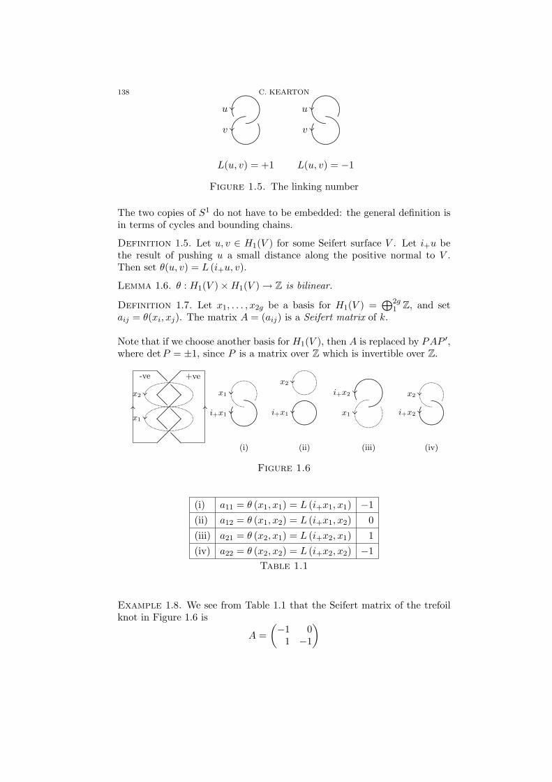
138 C. KEARTON
L(u, v) = +1
................
................
u
v
..............................................................................................................................................................................................................................
...............................................................
.............................................................................................................
L(u, v) = −1
................
................
u
v
..........................................................................................................................................................
........................................... ....................................
.................................................................................................................................................................
Figure 1.5. The linking number
The two copies of S1 do not have to be embedded: the general definition isin terms of cycles and bounding chains.
Definition 1.5. Let u, v ∈ H1(V ) for some Seifert surface V . Let i+u bethe result of pushing u a small distance along the positive normal to V .Then set θ(u, v) = L (i+u, v).
Lemma 1.6. θ : H1(V )×H1(V ) → Z is bilinear.
Definition 1.7. Let x1, . . . , x2g be a basis for H1(V ) =⊕2g
1 Z, and setaij = θ(xi, xj). The matrix A = (aij) is a Seifert matrix of k.
Note that if we choose another basis for H1(V ), then A is replaced by PAP ′,where detP = ±1, since P is a matrix over Z which is invertible over Z.
............................................................................................ ............................................................................................ ............................................................................................
................................................................................................................................................................................................................................................
.............. ..............
..............
..............
x2
x1
+ve-ve.................................................................................
.......................
......................
........................
.................
.....................................................................................
(i)
................
................
x1
i+x1
.................................................................................................................................................
....................................... ...............
...........................................................
(ii)
..............
..............
x2
i+x1
........................................................................................................................................
.............................................................
..................
..........................
..............................................
(iii)
................
................
i+x2
x1
........................................................................................................
...............................................................
.............................................................................................................
(iv)
..............
..............
x2
i+x2
........................................................................................................................................
................................... ..............
......................
.................................
Figure 1.6
(i) a11 = θ (x1, x1) = L (i+x1, x1) −1(ii) a12 = θ (x1, x2) = L (i+x1, x2) 0(iii) a21 = θ (x2, x1) = L (i+x2, x1) 1(iv) a22 = θ (x2, x2) = L (i+x2, x2) −1
Table 1.1
Example 1.8. We see from Table 1.1 that the Seifert matrix of the trefoilknot in Figure 1.6 is
A =(−1 0
1 −1
)
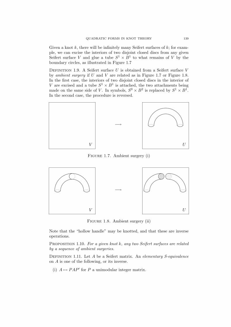
QUADRATIC FORMS IN KNOT THEORY 139
Given a knot k, there will be infinitely many Seifert surfaces of k; for exam-ple, we can excise the interiors of two disjoint closed discs from any givenSeifert surface V and glue a tube S1 × B1 to what remains of V by theboundary circles, as illustrated in Figure 1.7
Definition 1.9. A Seifert surface U is obtained from a Seifert surface Vby ambient surgery if U and V are related as in Figure 1.7 or Figure 1.8.In the first case, the interiors of two disjoint closed discs in the interior ofV are excised and a tube S1 × B1 is attached, the two attachments beingmade on the same side of V . In symbols, S0 × B2 is replaced by S1 × B1.In the second case, the procedure is reversed.
V
−→ ...............................................................
...............................
.............................................................................................................................................. .............................................................................
.......................
...............................
............................................................................................................................................................................................................................... ..........................................
..............................................
..............
U
Figure 1.7. Ambient surgery (i)
........
.......................................................
...............................
.............................................................................................................................................. ..............................................................................
.......................
...............................
.............................................................................................................................................................................................................................. ..........................................
..........................................
...........................................................
.............
.....
............
V
−→ ...............................................................
...............................
........................
........
......................................................................................
........................
........
........
..............................................................
.......................
...............................
.............................................
........
........
....................................................................................................................
.............................................
....................................................................................
...........................................................
......................................................................................................................
.............
.....
.........................
..
..
..
..
..
..
.
..
..
..
.
..
..
..
.
..
..
..
.
..
..
..
.
..
..
..
..
..
....... .
.
.
....
.
.
.
.
.
.
....
U
Figure 1.8. Ambient surgery (ii)
Note that the “hollow handle” may be knotted, and that these are inverseoperations.
Proposition 1.10. For a given knot k, any two Seifert surfaces are relatedby a sequence of ambient surgeries.
Definition 1.11. Let A be a Seifert matrix. An elementary S-equivalenceon A is one of the following, or its inverse.
(i) A 7→ PAP ′ for P a unimodular integer matrix.

140 C. KEARTON
(ii)
A 7→
A 0 0α 0 00 1 0
(iii)
A 7→
A β 00 0 10 0 0
where α is a row vector of integers and β is a column vector of integers.
Two matrices are S-equivalent if they are related by a finite sequence of suchmoves.
Theorem 1.12. Any two Seifert matrices of a given knot k are S-equivalent.
Proof. Let A be the matrix obtained from a Seifert surface U , B fromV . After Proposition 1.10, it is enough to assume that V is obtained by anambient surgery on U . Consider the diagram in Figure 1.9, and choose gen-
U
−→ ...............................................................
...............................
.............................................................................................................................................. ..............................................................................
.......................
...............................
.............................................................................................................................................................................................................................. ..........................................
..............................................
.....................
................................................................................... .....
.....
...............................
.............
................................................................................................................. ........
........................
x2g+1x2g+2
V
Figure 1.9
erators x1, . . . , x2g of H1(U), and x1, . . . , x2g, x2g+1, x2g+2 of H1(V ). Then
θ (x2g+1, x2g+1) = 0 if we choose the right number of twists around the
handle (see Figure 1.10 for a different choice)
θ (x2g+1, x2g+2) = 0
θ (x2g+2, x2g+1) = 1
θ (x2g+2, x2g+2) = 0
θ (xi, x2g+2) = 0
θ (x2g+2, xi) = 0 for 1 ≤ i ≤ 2g.
Thus
B =
A γ 0α 0 00 1 0

QUADRATIC FORMS IN KNOT THEORY 141
U
−→ ...............................................................
...............................
.............................................................................................................................................. .............................................................................
.......................
...............................
............................................................................................................................................................................................................................... ..........................................
..............................................
.....................
................................................................................... .....
.....
...............................
.............
.....................
.....
.....
.....................................................
.........................
..............
..
..
..
..
........
........................
x2g+1x2g+2
V
Figure 1.10
By a change of basis we can subtract multiples of the last row from the first2g rows to eliminate γ; and the same multiples of the last column from thefirst 2g columns. Whence
P ′BP =
A 0 0α 0 00 1 0
Adding the handle on the other side of U gives the other kind of S-equivalence.¤
Lemma 1.13. If A is a Seifert matrix and A′ is its transpose, then A − A′is unimodular.
Proof. Recall that if x1, . . . , x2g is a basis for H1(V ) =⊕2g
1 Z, andaij = θ(xi, xj), then the matrix A = (aij) is a Seifert matrix of k. Let i−ube the result of pushing u a small distance along the negative normal to V .Then
aij = θ(xi, xj)
= L (i+xi, xj)
= L (xi, i−xj)
= L (i−xj , xi)
and so
aij − aji = L (i+xi, xj)− L (i−xi, xj) = L (i+xi − i−xi, xj)
Now i+xi− i−xi is the boundary of a chain S1× I normal to V which meetsV in xi, and so L (i+xi − i−xi, xj) is the algebraic intersection of this chainwith xj , i.e. the algebraic intersection of xi and xj in V . Hence A − A′represents the intersection pairing on H1(V ), whence the result. ¤
Now let us state what happens in higher dimensions.

142 C. KEARTON
Definition 1.14. A (2q − 1)-knot k is simple if its exterior K satisfiesπi (K) ∼= πi
(S1
)for 1 ≤ i < q.
The following result is proved in [33, Theorem 2].
Theorem 1.15. A (2q−1)-knot k is simple if and only if it bounds a (q−1)-connected Seifert submanifold.
Now suppose that k is a simple (2q−1)-knot bounding an (q−1)-connectedsubmanifold V . We can repeat the construction above, using Hq(V ), toobtain a Seifert matrix A of k satisfying the following.
Theorem 1.16. If A is a Seifert matrix of a simple (2q − 1)-knot k and A′is its transpose, then A + (−1)qA′ is unimodular. Moreover, if q = 2, thenthe signature of A + A′ is a multiple of 16.
Theorem 1.12 remains true for simple knots. The following result is provedin [41] for q = 1, in [36, Theorem 2] for q = 2, and in [31, Theoreme II.3]for q > 2.
Theorem 1.17. Let q be a positive integer and A a square integral matrixsuch that A + (−1)qA′ is unimodular and, if q = 2, A + A′ has signature amultiple of 16. If q 6= 2, there is a simple (2q−1)-knot k with Seifert matrixA. If q = 2, there is a simple 3-knot k with Seifert matrix S-equivalent toA.
In [36, Theorem 3] the classification of simple knots is completed.
Theorem 1.18. A simple (2q−1)-knot k, q > 1, is determined up to ambientisotopy by the S-equivalence class of its Seifert matrix.
2. Blanchfield Duality
Let us set Λ = Z[t, t−1
], the ring of Laurent polynomials in a variable t
with integer coefficients.
Theorem 2.1. If A is a Seifert matrix of a simple (2q − 1)-knot k, thenthe Λ-module MA presented by the matrix tA+(−1)qA′ depends only on theS-equivalence class of A, and so is an invariant of k. Moreover, there is anon-singular (−1)q+1-hermitian pairing
〈 , 〉A : MA ×MA → Λ0/Λ
given by the matrix (1− t) (tA + (−1)qA′)−1 which is also an invariant of k.Conjugation is the linear extension of t 7→ t−1, Λ0 is the field of fractions ofΛ, and non-singular means that the adjoint map MA → Hom(MA, Λ0/Λ) isan isomorphism.

QUADRATIC FORMS IN KNOT THEORY 143
Definition 2.2. The Λ-module in Theorem 2.1 is called the knot module ofk, and has a geometric significance which is explained in §6. The determi-nant of tA + (−1)qA′ is the Alexander polynomial of k, and is defined up tomultiplication by a unit of Λ. The hermitian pairing is due to R.C. Blanch-field [9]. The formula given here was discovered independently in [22, 44].
The following two results are proved in [22, 23, 44, 45].
Theorem 2.3. If A is a Seifert matrix of a simple (2q− 1)-knot k, then themodule and pairing (MA, 〈 , 〉A) satisfy:
(i) MA is a finitely-generated Λ-torsion-module;(ii) (t− 1) : MA → MA is an isomorphism;(iii) 〈 , 〉A : MA ×MA → Λ0/Λ is a non-singular (−1)q+1-hermitian pair-
ing.
For q = 2 the signature is divisible by 16. Moreover, for q > 1, the moduleand pairing determine the knot k up to ambient isotopy.
Theorem 2.4. Suppose that (M, 〈 , 〉) satisfies
(i) M is a finitely-generated Λ-torsion-module;(ii) (t− 1) : M → M is an isomorphism;(iii) 〈 , 〉 : M ×M → Λ0/Λ is a non-singular (−1)q+1-hermitian pairing.
and that, for q = 2, the signature is divisible by 16. Then for q ≥ 1,(M, 〈 , 〉) arises from some simple (2q − 1)-knot as (MA, 〈 , 〉A).
In [43, pp 485-489] Trotter proves the following.
Proposition 2.5. If A is a Seifert matrix, then A is S-equivalent to a matrixwhich is non-degenerate; that is, to a matrix with non-zero determinant.
Proposition 2.6. If A and B are non-degenerate Seifert matrices of asimple (2q − 1)-knot k, then A and B are congruent over any subring of Qin which detA is a unit. (Of course, det A is the leading coefficient of theAlexander polynomial of k.)
Definition 2.7. Let ε = (−1)q and let A be a non-degenerate Seifert matrixof a simple (2q − 1)-knot k. Set S = (A + εA′)−1 and T = −εA′A−1.
Proposition 2.8. The pair (S, T ) have the following properties:
(i) S is integral, unimodular, ε-symmetric;(ii) (I − T )−1 exists and is integral;(iii) T ′ST = S;(iv) A = (I − T )−1S−1.
The following result is proved in [44, p179]
Theorem 2.9. The matrix S gives a (−1)q-symmetric bilinear pairing ( , )on MA on which T (i.e. t) acts as an isometry. The pair (MA, ( , ))determines and is determined by the S-equivalence class of A.

144 C. KEARTON
3. Factorisation of Knots
If we have two classical knots, there is a natural way to take their sum:just tie one after another in the same piece of string. Alternatively, we canthink of each knot as a knotted ball-pair and identify the boundaries sothat the orientations match up. The latter procedure generalises to higherdimensions.
Definition 3.1. Let k1, k2 be two n-knots, say ki =(Sn+2
i , Sni
). Choose
a point on each Sni and excise a tubular neighbourhood, i.e. an unknotted
ball-pair, leaving a knotted ball-pair(Bn+2
i , Bni
). Identify the boundaries
so that the orientations match up, giving a sphere-pair k1 + k2.
If k1, k2 are simple knots with Seifert matrices A1, A2, then clearly k1 + k2
is also simple and has a Seifert matrix(A1 00 A2
)
and the pairings in §2 are given by the orthogonal direct sum.
For the case n = 1, H. Schubert showed in [40] that every knot factorisesuniquely as a sum of irreducible knots. In [25] it is shown that uniquefactorisation fails for n = 3, and in [1] E. Bayer showed that it fails forn = 5 and for n ≥ 7. The following example is contained in [1], althoughpresented here in a slightly different way.
Let Φ15(t) denote the 15th cyclotomic polynomial, which we normalise sothat Φ15(t) = Φ15
(t−1
), and let ζ = e
2πi15 . Then Z[ζ] ∼= Z
[t, t−1
]/ (Φ15(t))
is the ring of integers, and conjugation in Z[t, t−1
]corresponds to complex
conjugation in Z[ζ]. Moreover, ζ − 1 is a unit in Z[ζ], and so we can thinkof Z[ζ] as a Λ-module satisfying properties (i) and (ii) of Theorem 2.3. Ifu ∈ U0, the set of units of Z[ζ + ζ], then we can define a hermitian pairingon Z[ζ] by (x, y) = uxy. This corresponds to a hermitian pairing as inTheorem 2.3(iii) by
〈x(t), y(t)〉 =u(t)x(t)y
(t−1
)
Φ15(t)←→ (x(ζ), y(ζ)) = ux(ζ)y(ζ).
The case of skew-hermitian pairings is dealt with by using(ζ − ζ
)u in place
of u. Note that ζ − ζ is a unit:
(3.1)(ζ − ζ
)2 (ζ + ζ
) (1− ζ − ζ
)= 1.
Lemma 3.2. Let ur = ζr + ζ−r − 1 for r = 0, 1, 2, 7. Then ur ∈ U0 and(ur 00 −ur
)and
(1 00 −1
)
represent isometric pairings on Z[ζ]× Z[ζ].

QUADRATIC FORMS IN KNOT THEORY 145
Proof. Since ζ2, ζ7 are also primitive 15th roots of unity, (3.1) showsthat ur ∈ U0 for r = 1, 2, 7. Of course, u0 = 1. Now consider
(a bb a
)(1 00 −1
) (a bb a
)=
(aa− bb 0
0 bb− aa
)=
(ur 00 −ur
)
For each r, we can write
ur = ζr + ζ−r − 1 = 1− (ζr − 1)(ζ−r − 1
)
and so we can take a = 1, b = (ζr − 1). ¤
Lemma 3.3. The hermitian forms on Z[ζ] given by ±ur for r = 0, 1, 2, 7 aredistinct.
Proof. Two such forms represented by u, v ∈ U0 are equivalent if andonly if uv−1 ∈ N(U), where N(c) = cc; write u ∼ v to denote this equiv-alence. Then u1 > 0 but u1 is conjugate to u7 < 0, so ±u1 /∈ N(U) andhence the forms represented by ±1,±u1 are distinct. Similarly u2/u1 > 0but u2/u1 is conjugate to u4/u2 < 0, so ±u2/u1 /∈ N(U). Similar argumentsapply in the other cases. ¤
Corollary 3.4. For each q > 2 there exist eight distinct irreducible simple(2q − 1)-knots kr, k
−r , r = 0, 1, 2, 7, such that kr + k−r = ks + k−s for all
r, s ∈ 0, 1, 2, 7.
Proof. By Theorem 2.3 there exist unique simple (2q−1)-knots kr, k−r
corresponding to ur,−ur respectively. These are irreducible because in eachcase the Alexander polynomial is Φ15(t). ¤
Remark 3.5. It is shown in [1] that U0/N(U) has exactly eight elements,so that these are all the forms there are in this case.
There is another method, due to J.A. Hillman, depending upon the modulestructure, and this can be used to show that unique factorisation fails forn ≥ 3 (see [5]). There are further results on this topic in [18, 17, 19]. Itis known from [10] that every n-knot, n ≥ 3, factorises into finitely manyirreducibles, and that a large class of knots factorise into irreducibles in atmost finitely many different ways (see [6, 8]).
I should mention that the method of [25] relies on the signature of a smooth3-knot being divisible by 16, and hence does not generalise to higher dimen-sions. The work of Hillman in [20] shows that the classification theorems1.16, 1.17, 1.18, and 2.3 hold for locally-flat topological 3-knots without anyrestriction on the signature.
146 C. KEARTON
4. Cancellation of Knots
In [3] Eva Bayer proves a stronger result, that cancellation fails for simple(2q − 1)-knots, q > 1.
Example 4.1. Let A be the ring of integers associated with Φ12, and defineΓ4n to be the following lattice given in [39]. We take R4n to denote theeuclidean space, and let e1, . . . , e4n be an orthonormal basis with respectto the usual innerproduct. Then Γ4n is the lattice spanned by the vectorsei + ej and 1
2 (e1 + · · ·+ e4n). Let AΓ4n be the corresponding hermitianlattice. It is shown in [3] that the hermitian form AΓ4n is irreducible ifn > 1. Moreover
(4.1) AΓ8 ⊥ AΓ8 ⊥< −1 >∼= AΓ16 ⊥< −1 >;
indeed, this holds already over Z by [39, Chap. II, Proposition 6.5]. ButAΓ8 ⊥ AΓ8 6∼= AΓ16 because the latter is irreducible. By Theorem 2.1 thisshows that cancellation fails for q odd, q 6= 1. For q even, just multiply 4.1by the unit τ − τ−1 where τ is a root of Φ12.
In [4], examples are given where the failure of cancellation depends on thestructure of the knot module, and by the device known as spinning thisresult is extended to even dimensional knots. (See §7 for the definition ofspinning.)
5. Knot Cobordism
There is an equivalence relation defined on the set of n-knots as follows.
Definition 5.1. Two n-knots ki =(Sn+2
i , Sni
)are cobordant if there is a
manifold pair(Sn+2 × I, V
)such that
V ∩ (Sn+2 × i) = ∂V ∩ (
Sn+2 × i) = Sni
(with the orientations reversed for i = 0) and Sni → V is a homotopy
equivalence for i = 0, 1.
Remark 5.2. For n ≥ 6 the manifold V is a product, i.e. it is homeomorphicto Sn × I, by the h-cobordism theorem.
This equivalence relation respects the operation of knot sum, and the equiva-lence classes form an abelian group Cn under this operation, with the trivialknot as the zero. In [31] M.A. Kervaire shows that C2q = 0 for all q.
To tackle the odd-dimensional case, we begin by quoting a result of Levine:[35, Lemma 4].
Lemma 5.3. Every (2q − 1)-knot is cobordant to a simple knot.

QUADRATIC FORMS IN KNOT THEORY 147
Definition 5.4. Let A0, A1 be two Seifert matrices of simple (2q−1)-knots.
If(−A0 0
0 A1
)is congruent to one of the form
(0 N1
N2 N3
)where each of the
Ni are square of the same size then A0, A1 are said to be cobordant. Thisis an equivalence relation for Seifert matrices, and the set of equivalenceclasses forms a group under the operation induced by taking the block sum:
(A0, A1) 7→(
A0 00 A1
).
Lemma 5.5. Let k0, k1 be simple (2q − 1)-knots which are cobordant, withSeifert matrices A0, A1 respectively. Then A0, A1 are cobordant.
From Proposition 2.5 we deduce:
Corollary 5.6. Every Seifert matrix is cobordant to a non-degenerate ma-trix.
Definition 5.7. Setting εq = sign (−1)q, the group obtained from theSeifert matrices of simple (2q − 1)-knots is denoted by Gεq . The subgroupof G+ given by matrices A such that the signature of A + A′ is divisible by16 is denoted G0
+. The map ϕq : C2q−1 → Gεq is induced by taking a simpleknot to one of its Seifert matrices, and is a homomorphism.
The definition above appears in [35], where the following result is proved.
Theorem 5.8. The map ϕq is
(a) an isomorphism onto Gεq for q ≥ 3;(b) an isomorphism onto G0
+ for q = 2;(c) an epimorphism onto G− for q = 1.
The proof of [34, Lemma 8] shows that two Seifert matrices are cobordantif and only if they are cobordant over the rationals. This leads to the idea ofWitt classes for the (−1)q-symmetric forms and isometries in Theorem 2.9,and this is the strategy that Levine uses to investigate Gε, and to proveTheorem 5.9 below (see [35, p 108]).
Theorem 5.9. Gε is the direct sum of cyclic groups of orders 2, 4 and ∞,and there are an infinite number of summands of each of these orders.
Both Levine’s treatment and that of Kervaire in [32] rely on Milnor’s clas-sification of isometries of innerproduct spaces in terms of hermitian formsin [38].
I shall not attempt to prove any of these results, but it is easy to giveMilnor’s proof in [37] of infinitely many summands of infinite order for qodd, and at the same time to suggest an alternative way of looking at Gεq .First make the following definition, taken from [24].
148 C. KEARTON
Definition 5.10. A module and pairing (MA, < , >A) as in Theorem 2.1is null-cobordant if there is a submodule of half the dimension of MA whichis self-annihilating under < , >A. And (MA, < , >A), (MB, < , >B) arecobordant if the orthogonal direct sum A ⊥ (−B) is null-cobordant. Thedimension of MA is the dimension over Q of MA after passing to rationalcoefficients.
It is shown in [24] that (MA, < , >A) is null-cobordant if and only if A isnull-cobordant. If we use rational coefficients, which we may as well do inlight of [34, Lemma 8], the proof is even easier. We shall treat (MA, < , >A)in this way for the rest of this section, and set Γ = Q
[t, t−1
].
Definition 5.11. Given p(t) ∈ Λ, define p∗(t) = tdeg(p(t))p(t−1
). And for
an irreducible p(t) ∈ Λ define MA(p(t)) to be the p-primary component ofMA, i.e. the submodule annihilated by powers of p(t).
The following result is essentially Cases 1 and 3 of [38, p93, Theorem 3.2]:note that Case 2 does not arise here since we are dealing with knot modules,i.e. p(t) 6= t± 1.
Proposition 5.12. (MA, < , >A) splits as the orthogonal direct sum ofMA(p(t)) where p(t) = p∗(t), and of MA(p(t)) ⊕ MA(p∗(t)) where p(t) 6=p∗(t). Furthermore, for p(t) = p∗(t) the space MA(p(t)) splits as an orthog-onal direct sum M1 ⊕M2 ⊕ . . . where M i is annihilated by p(t)i but is freeover the quotient ring Γ/p(t)iΓ.
It is slightly easier to prove [38, Theorem 3.3] here.
Theorem 5.13. When p(t) = p∗(t), for each i, the vector space
H i = M i/p(t)M i
over the field E = Γ/p(t)Γ admits one and only one hermitian inner product((x), (y)) such that
(5.1)⟨p(t)i−1x, y
⟩=
a(t)p(t)
←→ ((x), (y)) = a(ζ)
where (x) denotes the image of x ∈ M i in H i. The sequence of these her-mitian inner product spaces determines (MA(p(t)), < , >) up to isometry.
The following is easy to prove, where we think of the hermitian form on H i
as taking values in Γ0/Γ.
Lemma 5.14. For i even, M i is null-cobordant. For i odd, M i is cobordantto H i.
This enables us to make the following definition of the Milnor signatures(compare [38]).

QUADRATIC FORMS IN KNOT THEORY 149
Definition 5.15. For each p(t) = p∗(t), define
σp =∑
i odd
σi,
where σi is the signature of H i.
Lemma 5.16. The signature σp is additive over knot composition and zerowhen k is null-cobordant, and so is a cobordism invariant.
Example 5.17 (Milnor, [37]). For each positive integer m, let pm(x) =mt+(1−2m)+mt−1. Then pm is irreducible and is the Alexander polynomial
of a simple (4q + 1)-knot km for each q ≥ 1 having(
m 10 1
)as a Seifert
matrix. Then σpm = ±2 for each m, and so for each q ≥ 1 we have infinitelymany independent knots of infinite order in C4q+1.
6. Branched Cyclic Covers
Recall that if k is an n-knot(Sn+2, Sn
), then a regular neighbourhood of Sn
has the form Sn ×B2, and the exterior of k is K = Sn+2 − int(Sn ×B2
).
Choose a base-point ∗ ∈ K. By Alexander-Poincare duality, K has thehomology of a circle, and so the Hurewicz theorem gives a map π1(K, ∗) ³H1(K) whose kernel is the commutator subgroup [π1(K, ∗), π1(K, ∗)] of thegroup π1(K, ∗). We write the infinite cyclic group H1(K) multiplicatively,as (t : ); the generator t is represented by a×S1 ⊂ Sn×S1 = ∂K for somepoint a ∈ Sn, and is chosen so that the oriented circle has linking number+1 with Sn.
Let K → K be the infinite cyclic cover corresponding to the kernel of theHurewicz map. A triangulation of K lifts to a triangulation of K on which(t : ) acts as the group of covering transformations. This induces an actionof (t : ) on the chain complex C∗(K), which extends by linearity to makeC∗(K) a Λ = Z[t, t−1]-module. The Λ-module C∗(K) is finitely-generatedbecause the original triangulation of K is finite. Passing to homology weobtain H∗(K) as a finitely-generated, indeed finitely-presented, Λ-module.For a simple (2q−1)-knot, the only non-trivial module is Hq(K), and this isin fact the same as the Λ-module MA presented by the matrix tA+(−1)qA′in Theorem 2.1.
To recover K from K all we do is identify x with tx, for each x ∈ K.
Compose the Hurewicz map with the map sending (t : ) onto the finitecyclic group of order r, and denote the r-fold cover of K corresponding tothe kernel of this map by Kr. Since ∂Kr ∼= Sn × S1, being an r-fold coverof Sn × S1, we may set Kr = Kr ∪∂
(Sn ×B2
)to obtain the r-fold cover
of Sn+2 branched over Sn. It may happen that Kr ∼= Sn+2, in which casewe have another n-knot kr, which we refer to as the r-fold branched cyclic

150 C. KEARTON
cover of k. In this case H∗(K) is a Z [tr, t−r]-module when K is regarded asthe infinite cyclic cover of Kr. Note that kr is the fixed point set of the Zr
action on Sn+2 = Kr given by the covering transformations.
Let k be a simple (2q− 1)-knot giving rise to a pair of matrices (S, T ) as inProposition 2.8, and define U, V by
U =
0 . . . 0 T
I. . . 0. . . . . .
...0 I 0
V =
S 0 . . . 0
0. . .
......
. . . 00 . . . 0 S
there being r × r blocks in each case. It is not hard to show that the pair(V, U) satisfies the conditions of Proposition 2.8, and so corresponds to aunique simple (2q − 1)-knot kr if q ≥ 2 (see Theorem 2.9). Moreover,
U r =
T 0 . . . 0
0. . .
......
. . . 00 . . . 0 T
from which it follows without much difficulty that the r-fold branched cycliccover of kr is #r
1k, the sum of r copies of k.
The topological construction of kr may be described as follows. Take aSeifert surface W of k which meets a tubular neighbourhood N of k in acollar neighbourhood of k = ∂W . Take r close parallel copies W1, . . . , Wr ofW , so that the space between Wi and Wi+1 is diffeomorphic to W × [0, 1]for i = 1, . . . , r − 1, and that between Wr and W1 is diffeomorphic to theexterior of k split open along W . We can join ∂Wi to ∂Wi+1 for 1 ≤ i ≤ r−1by bands within N to get the the boundary connected sum of the Wi. Thenit is not hard to see that the Seifert surface we have constructed has V, Uas above. Moreover, for q > 1, the resulting knot kr is independent of thebands used, since the bands unknot in these dimensions.
In [29] examples are given of simple (2q − 1)-knots k, l, q ≥ 2, for which#r
1k = #r1l but kr 6= lr. It is known that there are examples for any odd r.
The argument runs as follows.
Let Φm(t) denote the mth cyclotomic polynomial, where m is divisible byat least two distinct odd primes, and let ζ be a primitive mth root of unity.We write K = Q(ζ) and F = Q
(ζ + ζ−1
). Let hK denote the class number
of K, hF that of F, and h− = hK/hF. According to the work of Eva Bayerin [2], the number of distinct simple (2q − 1)-knots, q ≥ 3, with Alexanderpolynomial Φm(t) is h−2d−1 where 2d = ϕ(m) = [K : Q]. The factor h−represents the number of isomorphism classes of Λ-modules supporting aBlanchfield pairing [2, Corollary 1.3], and the factor 2d−1 represents thenumber of pairings (up to isometry) which a given module supports. The
QUADRATIC FORMS IN KNOT THEORY 151
latter is in one-one correspondence with U0/N(U) where U is the group ofunits in (the ring of integers of) K, U0 the group of units of F, and N : K→ Fis the norm.
If h− has an odd factor r > 1 coprime to m, then there exists an ideal aof Q(ζ) which has order r in the class group and supports a unimodularhermitian pairing h, i.e. as a Λ-module it supports a Blanchfield pairing.Then ⊥r
1 (a, h) has determinant (I, u) for some u ∈ U0/N(U), where Idenotes a principal ideal. Since r is odd and |U0/N(U)| = 2d−1, there existsv ∈ U0/N(U) such that vr = u.
Let k, l be the simple (2q − 1)-knots, q ≥ 2, corresponding to κ = (a, h) ⊥(a,−h), λ = (I, v) ⊥ (I,−v) respectively. Then ⊥r
1 κ, ⊥r1 λ are indefinite
and have the same rank, signatures and determinant. Hence by [2, Corollary4.10] they are isometric, and so #r
1k = #r1l. But κ is not isometric to λ,
for the determinant of κ is(a2, α
)for some α, and a2 is non-zero in the
ideal class group since r is odd. Hence k 6= l. A similar, but more involved,argument shows that kr 6= lr.
Many examples may be obtained from the tables in [46] or [47].
7. Spinning and Branched Cyclic Covers
First we recall a definition of spinning. Let k be the n-knot(Sn+2, Sn
)and
let B be a regular neighbourhood of a point on Sn such that (B,B ∩ Sn) isan unknotted ball pair. Then the closure of the complement of B in Sn+2 isa knotted ball pair
(Bn+2, Bn
), and σ(k) is the pair ∂
[(Bn+2, Bn
)×B2].
The following is proved in [28, Theorem 3].
Theorem 7.1. Let k, l be simple (2q − 1)-knots, q ≥ 3; then σ(k) = σ(l) ifand only if Hq(K) ∼= Hq(L).
Note that [28] only covers the case q ≥ 5; the theorem is extended to q ≥ 3by the results of [21].
In [7] it is shown that the following holds.
Proposition 7.2. If q ≥ 4, then the map σ acting on simple (2q− 1)-knotsis finite-to-one.
The following is easy to prove (see [30, Lemma 3.1]).
Lemma 7.3. Let k be an n-knot and r an integer such that the r-fold cycliccover of Sn+2 branched over k is a sphere. Then the r-fold cyclic cover ofSn+3 branched over σ(k) is also a sphere, and σ (kr) = σ(k)r.
In [42], Strickland proves the following result.

152 C. KEARTON
Theorem 7.4. Let k be a simple (2q − 1)-knot, q ≥ 2. Then k is the r-foldbranched cyclic cover of a knot if and only if there exists an isometry u of(Hq(K), < , >
)such that ur = t.
A careful reading of [42] shows that the same proofs apply, almost verbatim,to yield the following result (see [30, Theorem 2.5]).
Theorem 7.5. Let k be a simple (2q − 1)-knot, q ≥ 5. Then σ(k) is ther-fold branched cyclic cover of a knot if and only if there is a Λ-moduleisomorphism u : Hq(K) → Hq(K) such that ur = t.
Thus if we can find a simple (2q − 1)-knot k, q ≥ 5, such that there is a Λ-module isomorphism u : Hq(K) → Hq(K) with ur = t, but no such isometryof Hq(K), then σ(k) will be the r-fold branched cyclic cover of a knot but kwill not. Examples of such knots are given in [30] for all q ≥ 5 and all evenr. Here is an example, due to S.M.J. Wilson, much simpler than the onesin [30] but not capable of generalising to the 2r-fold case.
Example 7.6. Let f(t) = t2 − 3t + 1, which has roots 3±√52 . Set τ = 3+
√5
2 ,ξ = 1+
√5
2 , and note that ξ2 = τ . Put R = Z [ξ] = Z[τ, τ−1
]and define
conjugation in the obvious way by ξ = 1−√52 . Think of R as an R-module,
and put a hermitian form on it by setting (x, y) = xy. Since ξξ = −1, ξ is anisomorphism on R but not an isometry. Since τ only has two square roots,±ξ, there are no isometries whose square is τ . In the usual way, (R, ( , ))corresponds to a knot module and pairing for a simple (4q + 1)-knot, q > 1.
8. Concluding Remarks
So far we have only dealt with odd dimensional knots, but much of what hasbeen said can be extended to even dimensions. By Proposition 1.1, every 2q-knot k bounds an orientable (2q+1)-manifold V in S2q+2. A simple 2q-knotk is one for which there is a (q−1)-connected V , so that Hq(V ) and Hq+1(V )
are the only non-trivial homology groups. Then Hq
(K
), Hq+1
(K
)are the
only non-trivial homology modules. There is a sesquilinear duality pairingon Hq
(K
)×Hq+1
(K
), and this, together with some more algebraic struc-
ture connecting them, can be used to classify the simple 2q-knots in highdimensions. See [13, 14, 15, 26, 27] for details.
Classification results have also been obtained for more general classes ofknots; see [11, 12, 16].
References
[1] E. Bayer, Factorisation in not unique for higher dimensional knots, Comm. Math.Helv. 55 (1980), 583–592.
QUADRATIC FORMS IN KNOT THEORY 153
[2] , Unimodular hermitian and skew-hermitian forms, Jour. of Algebra 74 (1982),341–373.
[3] , Definite hermitian forms and the cancellation of simple knots, Archiv derMath. 40 (1983), 182–185.
[4] , Cancellation of hyperbolic ε-hermitian forms and of simple knots, Math.Proc. Camb. Phil. Soc. 98 (1985), 111–115.
[5] E. Bayer, J.A. Hillman, and C. Kearton, The factorization of simple knots, Math.Proc. Camb. Phil. Soc. 90 (1981), 495–506.
[6] E. Bayer-Fluckiger, C. Kearton, and S.M.J. Wilson, Decomposition of modules, formsand simple knots, Journal fur die reine und angewandte Mathematik 375/376 (1987),167–183.
[7] , Finiteness theorems for conjugacy classes and branched cyclic covers of knots,Mathematische Zeitschrift 201 (1989), 485–493.
[8] , Hermitian forms in additive categories: finiteness results, Journal of Algebra123 (1989), 336–350.
[9] R.C. Blanchfield, Intersection theory of manifolds with operators with applications toknot theory, Annals of Maths (2) 65 (1957), 340–356.
[10] M.J. Dunwoody and R.R. Fenn, On the finiteness of higher knot sums, Topology 26(1986), 337–343.
[11] M.Sh. Farber, Duality in an infinite cyclic covering and even-dimensional knots,Math. USSR Izvestija 11 (1977), no. 4, 749–781.
[12] , Isotopy types of knots of codimension two, Trans. Amer. Math. Soc. 261(1980), 185–209.
[13] , The classification of simple knots, Russian Math. Surveys 38 (1983), 63–117.[14] , An algebraic classification of some even-dimensional spherical knots. I,
Trans. Amer. Math. Soc. 281 (1984), no. 2, 507–527.[15] , An algebraic classification of some even-dimensional spherical knots. II,
Trans. Amer. Math. Soc. 281 (1984), no. 2, 529–570.[16] , Minimal Seifert manifolds and the knot finiteness theorem, Israel Journal of
Mathematics 66 (1989), no. 1–3, 179–215.[17] J.A. Hillman, Blanchfield pairings with squarefree Alexander polynomials, Math. Zeit.
176 (1981), 551–563.[18] , Finite knot modules and the factorization of certain simple knots, Math.
Annalen 257 (1981), 261–274.[19] , Factorization of Kojima knots and hyperbolic concordance of Levine pairings,
Houston Journal of Mathematics 10 (1984), 187–194.[20] , Simple locally flat 3-knots, Bull. Lond. Math. Soc. 16 (1984), 599–602.[21] J.A. Hillman and C. Kearton, Seifert matrices and 6-knots, Transactions of the Amer-
ican Mathematical Society 309 (1988), 843–855.[22] C. Kearton, Classification of simple knots by Blanchfield duality, Bulletin of the Amer-
ican Mathematical Society 79 (1973), 952–955.[23] , Blanchfield duality and simple knots, Transactions of the American Mathe-
matical Society 202 (1975), 141–160.[24] , Cobordism of knots and Blanchfield duality, Journal of the London Mathe-
matical Society 10 (1975), 406–408.[25] , Factorisation is not unique for 3-knots, Indiana University Mathematics
Journal 28 (1979), 451–452.[26] , An algebraic classification of certain simple knots, Archiv der Mathematik
35 (1980), 391–393.[27] , An algebraic classification of certain simple even-dimensional knots, Trans-
actions of the American Mathematical Society 276 (1983), 1–53.[28] , Simple spun knots, Topology 23 (1984), 91–95.

154 C. KEARTON
[29] C. Kearton and S.M.J. Wilson, Cyclic group actions on odd-dimensional spheres,Comm. Math. Helv. 56 (1981), 615–626.
[30] , Spinning and branched cyclic covers of knots, Royal Society of London Pro-ceedings A 455 (1999), 2235–2244.
[31] M.A. Kervaire, Les noeuds de dimensions superieures, Bull. Soc. math. France 93(1965), 225–271.
[32] , Knot cobordism in codimension 2, Manifolds Amsterdam 1970, Lecture Notesin Mathematics, vol. 197, Springer Verlag, Berlin-Heidelberg-New York, 1971, pp. 83–105.
[33] J. Levine, Unknotting spheres in codimension two, Topology 4 (1965), 9–16.[34] , Invariants of knot cobordism, Invent. math. 8 (1969), 98–110.[35] , Knot cobordism groups in codimension two, Comm. Math. Helv. 44 (1969),
229–244.[36] , An algebraic classification of some knots of codimension two, Comm. Math.
Helv. 45 (1970), 185–198.[37] J.W. Milnor, Infinite cyclic coverings, Conference on the Topology of Manifolds (ed.
J.G. Hocking), Complementary Series in Mathematics, vol. 13, Prindle, Weber &Schmidt, 1968, pp. 115–133.
[38] , On isometries of inner product spaces, Invent. math. 8 (1969), 83–97.[39] J.W. Milnor and D. Husemoller, Symmetric bilinear forms, Springer-Verlag, Berlin-
Heidelberg-New York, 1973.[40] H. Schubert, Die eindeutige Zerlegbarkeit eines Knotens in Primknoten, S.-B. Hei-
delberger Akad. Wiss. Math.-Natur. Kl. 1 3 (1949), 57–104.
[41] H. Seifert, Uber das Geschlecht von Knoten, Math. Ann. 110 (1934), 571–592.[42] Paul Strickland, Branched cyclic covers of simple knots, Proc. Amer. Math. Soc. 90
(1984), 440–444.[43] H.F. Trotter, Homology of group systems with applications to knot theory, Annals of
Math. 76 (1962), 464–498.[44] , On S-equivalence of Seifert matrices, Invent. math. 20 (1973), 173–207.[45] , Knot modules and Seifert matrices, Knot Theory, Proceedings, Plans-sur-
Bex 1977 (Berlin-Heidelberg-New York) (J.-C. Hausmann, ed.), Lecture Notes inMathematics, vol. 685, Springer-Verlag, 1978, pp. 291–299.
[46] G. Schrutka v. Rechtenstamm, Tabelle der (relativ-) Klassenzahlen von Kreiskorpern,Abh. Deutsch Akad. Wiss. Berlin 2 (1964), 1–64.
[47] L.C. Washington, Introduction to cyclotomic fields, Graduate Texts in Mathematics,vol. 83, Springer-Verlag, New York-Heidelberg-Berlin, 1982.
[48] E.C. Zeeman, Twisting spun knots, Trans. Amer. Math. Soc. 115 (1965), 471–495.
Mathematics DepartmentUniversity of DurhamSouth RoadDurham DH1 3LE, England
E-mail address: [email protected]

Contemporary Mathematics
Biography of Ernst Witt (1911-1991)
Ina Kersten
Abstract. Ernst Witt (1911–1991) was one of the most important influenceson the development of quadratic forms in the 20th century. His collected papers[CP] were published in 1998, but for copyright reasons without a biography.This article repairs the omission.
1. Childhood and youth
The grandfather of Ernst Witt, Heinrich Witt (1830–1893) worked as schoolteacher, author and lay preacher. He made his name as the author of three volumesof biblical commentary1. Many years later, his grandchildren were educated fromthese books. Heinrich Witt became widely known for his engagement in religiouseducation, including seminars for adults and Bible classes, held in the spirit ofthe widespread religious revivalist movement of the 19th century. He sacrificedeverything for his faith, expecting the same from his family. His children had totake second place to his great task.
1Die biblischen Geschichten Alten und Neuen Testaments mit Bibelwort und freier Zwi-schenrede anschaulich dargestellt (Biblical Histories From the Old and the New Testament, Illus-trated by Quotations from the Bible and Devotional Commentaries), published by BertelsmannGutersloh, 8 Marks.
c©0000 (copyright holder)
155

156 INA KERSTEN
This was the spiritual atmosphere into which Ernst Witt’s father Heinrich(1871–1959) was born, the seventh of thirteen children. Like nearly all of his broth-ers and sisters, he decided to join the Christian Movement. He studied theologyin Halle (Saale) with the intention of becoming a missionary. In 1893 a personalmeeting with Hudson Taylor (1832–1905), the founder of the China Home Mission,became a crucial aspect of his future life. In 1896, Heinrich Witt was appointed asthe travelling secretary of the German Christian Student Association, of which hewas a co-founder.
In 1900, the mission of Liebenzell, a German branch of the China Home Mission,sent him to China. There he adopted Chinese customs wearing Chinese clothesand plaiting his hair in order to gain the confidence of the local people. He totallysubmitted himself to the principles of Taylor and always did as he was instructed,distributing tracts, selling books and brochures and holding street meetings. In1906, he married Charlotte Jepsen from Sonderburg (which is now in Denmark)where he had done his voluntary military service eleven years before. The couplemoved to a small, moderately furnished rice farmer’s hut in Yuanchow. In spiteof the primitive conditions, they were content. As the mission of Liebenzell wasvery poor, the missionaries did not receive a fixed salary and had to get by on barenecessities.
In 1911, they were granted their first home leave. With their three-year-olddaughter they went back to Germany, where Heinrich Witt worked again as atravelling secretary until 1913. Their son Ernst was born on June 26, 1911 onAlsen, a Baltic Sea island, which was German at that time.
As a child of missionaries, an unusual fate awaited him. At the age of two hecame to China, where his father became superintendent and head of the LiebenzellMission in Changsha. A high wall closed off the mission station, Ernst’s home forthe following years, from the hostile outside world. Heinrich Witt often went forlong journeys and did not have much time for his children – there were to be six inall. They were educated strictly; above all, the father attached great importanceto honesty. His eldest son Ernst, being without any playmates of the same age,was mostly left to himself. He had a passion for any kind of machine, and learntChinese from his Chinese nannies. His received his first lessons from his father, whorealized and promoted his son’s great talent for arithmetic. The father neglectedalmost all other subjects, for lack of time. However, he studied with his sons, Ernstand Otto, all of the biblical histories by Heinrich Witt mentioned at the beginningof this article.
When Ernst Witt was nearly nine years old, he and his younger brother Ottowere sent to Germany for their schooling. A brother of their father was to take careof their further education. They were sent to their uncle’s house at Mullheim, inthe south of Baden, where their elder sister had already been living for some time.The uncle was a preacher with eight children of his own. In due course he becamethe housemaster of a children’s home which had at times from 20–25 children ofmissionaries. His pedagogical work overwhelmed him and he ran a strict regimen.But he could not break the individualistic spirit of the young Ernst. In later yearsErnst Witt still used to stand by his convictions determinedly and consistently.Besides, he had a dry sense of humour which he retained his whole life. He alwaystook a keen pleasure in making other people laugh.

BIOGRAPHY OF ERNST WITT (1911-1991) 157
Ernst Witt visited the Realschule (grammar school) at Mullheim, where he wasmainly interested in mathematics and chemistry. After his mittlere Reife he wentto the Oberrealschule (high school) leading to the Abitur, the university entrancequalification – in Freiburg. There his class teacher was Karl Ottinger, an excellentmathematician, who discerned the extraordinary mathematical talent of his pupiland advanced him wherever he could. Ernst Witt maintained contact with thisteacher after his schooldays, and decades later he remembered him with gratitude.
During his school years in Freiburg, Ernst’s parents came to Germany for asecond leave from 1927–29. When they went back to China, they left all of theirchildren in Germany. Again they could communicate only by letter. In the courseof the following years, Heinrich Witt endeavoured to stay in touch with his son. Hetried to convince his son of his way of religious thinking, without success. Ernstrejected the biblical faith represented by his father. But his early education hadshaped his character. He detested lying – honesty and straightforwardness werehis characteristic feature. He always said what he thought, without any diplomacy,often causing misunderstandings and even hostility, which later worried him a lot.
2. University studies
After having passed his final exams, the Abitur, in 1929, Ernst Witt started tostudy mathematics and physics. For the first two terms he stayed in Freiburg, wherehe attended lectures by Loewy, Bolza and Mie. From the summer term of 1930 tothe winter term of 1933/34 he studied in Gottingen, mainly under Herglotz, EmmyNoether, Weyl, and Franck and astronomy under Meyermann. He particularlyliked the lectures of Gustav Herglotz (1881–1953), who had an extremely broadknowledge and whose talks stood out because of their special clarity. Herglotz, forhis part, always followed the mathematical development of his student with interestand sympathy, and they maintained contact until Herglotz’s death.
Seminar Excursion, Gottingen: Bernays, Scherk, Schilling, Schwerdtfeger, Taussky,
Bannow, Noether, –, W. Weber. Sitting: Witt, Ulm, –, –, Wichmann, Tsen, –.
158 INA KERSTEN
At the age of nineteen, Ernst Witt published his first paper including a newproof of Wedderburn’s theorem that every finite skew field is commutative [1931].Herglotz later remembered this ([6], 1946):
After one lecture, a young lad showed me a torn off piece of paper and said:‘This is a proof of Dickson’s theorem.’ In fact, it contained a proof of an extraordi-nary simplicity, not achieved up to then by any of the well-known mathematicians.When I got to know him closer, he showed an eminent mathematical gift, withwhich he, after a first approach, observed a thing in his own way and independentlyfollowed it to its furthest development.
In the summer of 1932, Emil Artin (1898–1962) came to Gottingen and heldhis famous lectures on class field theory, which strongly influenced Witt’s furtherscientific development. In the same year, Artin invited him to Hamburg, whereWitt intensively studied class field theory of number fields. In the course of thefollowing years, he carried the theory over to function fields [1934–36].
Witt had to study under extremely harsh economic conditions. He tried hardto keep his expenses to a minimum, taking special examinations for grants or theremission of tuition fees. He completed his Ph.D. after only four years, in thesummer of 1933. The title of his thesis was: Riemann-Rochscher Satz und Zeta-Funktion im Hyperkomplexen. The idea for it came to him through a problem setby Emmy Noether. She asked him whether the thesis by Artin’s student Kate HeyAnalytische Zahlentheorie in Systemen hyperkomplexer Zahlen could be transferredto algebraic function fields to find the hypercomplex analogue of the Riemann-Rochtheorem. Witt could answer Noether’s question in the affirmative by first proving,however, a Riemann-Roch theorem for central simple algebras over algebraic func-tion fields with perfect field of constants and then using this theorem to transferHey’s thesis.
As Witt liked to relate in later years, he wrote down his thesis within one week.In a letter of August 1933, his sister told her parents [2]:
He did not have a thesis topic until July 1, and the thesis was to be submittedby July 7. He did not want to have a topic assigned to him, and when he finally hadthe idea, [. . . ] he started working day and night, and eventually managed to finishin time. [. . . ] Artin also liked Ernst’s paper and has told him to go over it again,so that others might understand it as well.
The examiner of his thesis was Herglotz since Emmy Noether had been sus-pended from her duties by the Nazi regime. The oral examination held by Herglotz,Weyl, and Pohl was at the end of July 1933.
3. The time between 1933 and 1945
On 1st May, 1933 Ernst Witt joined the Nazi party and the SA, a step whichprovoked disappointment and bewilderment in the Gottingen mathematics insti-tute. By that time Emmy Noether was already suspended. Her seminar now tookplace at her home, where Witt turned up one day dressed in his SA uniform. Ap-parently, she did not take it amiss.
Herglotz later wrote in a report [6] of 22nd November, 1946:And then one day he had joined the S.A., urged by the simple wish – as I was
convinced in those days, and as I am still today – not to stand apart, where others
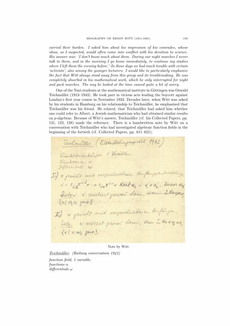
BIOGRAPHY OF ERNST WITT (1911-1991) 159
carried their burden. I asked him about his impression of his comrades, whoseideas, as I suspected, would often come into conflict with his devotion to science.His answer was: ‘I don’t know much about them. During our night marches I nevertalk to them, and in the morning I go home immediately, to continue my studieswhere I left them the evening before.’ In those days we had much trouble with certain‘activists’, also among the younger lecturers. I would like to particularly emphasizethe fact that Witt always stood away from this group and its troublemaking. He wascompletely absorbed in his mathematical work, which he only interrupted for nightand pack marches. The way he looked at the time caused quite a bit of worry.
One of the Nazi students at the mathematical institute in Gottingen was OswaldTeichmuller (1913–1943). He took part in vicious acts leading the boycott againstLandau’s first year course in November 1933. Decades later, when Witt was askedby his students in Hamburg on his relationship to Teichmuller, he emphasized thatTeichmuller was his friend. He related, that Teichmuller had asked him whetherone could refer to Albert, a Jewish mathematician who had obtained similar resultson p-algebras. Because of Witt’s answer, Teichmuller (cf. his Collected Papers, pp.121, 122, 138) made the reference. There is a handwritten note by Witt on aconversation with Teichmuller who had investigated algebraic function fields in thebeginning of the fortieth (cf. Collected Papers, pp. 611–621):
Note by Witt
Teichmuller. (Railway conversation 1942)
function field, 1 variable,functions αdifferentials ω

160 INA KERSTEN
I.) To find α with prescribed initial expansions.
α = ci−hπi−h + · · ·+ ci−1πi−1 + remainder α2 = α1 + α2. Divisor a2 .
Proposition. α exists if and only if∑
res α1 ω = 0 , ω | a2 ω integral.
II.) To find ω with prescribed initial parts.
Proposition. ω exists if and only if∑
res α ω1 = 0 , α | α w2 integral.
Witt did not take part in the political discussions during the years of 1933/34.But when in 1934 the university of Gottingen looked for a new head of the math-ematical institute and the students suggested a scientifically insignificant Nazi, heopenly expressed his indignation, despite threats by the SA.
In 1934, Witt became an assistant of Helmut Hasse (1898–1979) in Gottingen,where he qualified as a university lecturer in 1936. The oral exam took place inFebruary, his ‘habilitation lecture’ on convex bodies in June 1936. His ‘habilitation’on the theory of quadratic forms in arbitrary fields ranks as one of his most famousworks. In it he introduced what was later named the Witt ring of quadratic forms.Shortly after that, Witt introduced the ring of Witt vectors, which had a greatinfluence on the development of modern algebraic geometry (cf. G. Harder: “Anessay on Witt vectors” in [CP]).
Since Witt wanted to work as a lecturer, he had to attend and pass a compulsoryNational Socialist course for lecturers, which took place from August 2 to 28, 1937in Thuringen. At its end Witt received the following assessment [6]:National Socialist thinking: MediocreIndependent propagandist in any situation: NoNational Socialist disposition: LimitedPhysical capabilities: weakly-built, cannot be established because of a sporting injury.General enthusiasm for his duty: shirkerBehaviour towards people around him: quiet, restrained, his manners are somewhatinsecure.Description of his character: W. has shown himself to be quiet, modest and re-strained, with a tendency to keep to himself; characteristic features are a certainnaivety and eccentricity. He is honest and straightforward. He dedicates himself tohis work with dogged tenacity, continuously brooding and thinking and thus repre-sents the typical, politically indifferent researcher and scientist, who will probablybe successful in his subject, but who, at least for the time being, is lacking any ofthe qualities of a leader or educator.
This certificate just about allowed him to become a lecturer. It is striking howaccurate the ‘description of his character’ is. Some years later, Herglotz stressed(in his report of November 22, 1946), apart from Witt’s significant mathematicaltalent his striking unworldliness.
From 1933 until 1938 when he left Gottingen, Witt founded and organized astudy group on higher algebra and number theory. It produced seven importantpapers, all published in the celebrated volume 176 of the Crelle Journal.
BIOGRAPHY OF ERNST WITT (1911-1991) 161
In 1938, Ernst Witt became a lecturer at the mathematics department in Ham-burg, where, in 1939, he was appointed as an associate professor. He got the down-graded position of Emil Artin, who was forced to emigrate to the United States in1937. Witt’s move to Hamburg enabled him to break off his service in the SA.
In Hamburg, Witt met a fellow student, Erna Bannow, from Gottingen, whohad earlier gone to Hamburg to work with Artin. She continued her studies withWitt and finished her doctorate in 1939. A brief report on her thesis “Die Auto-morphismengruppen der Cayleyzahlen” (cf. Hamb. Abh. 13) was given by Witt inCrelles Journal. They married in 1940 and had two daughters.
In February 1940, Witt was called up by the Wehrmacht. He submitted hispaper on modular forms of degree two at the end of January 1940, thereby cuttingshort some of his investigations. In February 1940, with Blaschke’s help, he suc-ceeded in deferring his military service for one year. This enabled him to finish hispaper on reflection groups and the enumeration of semisimple rings, cf. [1941].
In February 1941, Witt came to Lubeck to be trained as a radio operator. Fromthere, in June 1941, he was sent to the Russian front. Later he said, that he had theworst time of his life there, and that he was surprised to survive it. In November1941, he fell ill and was sent back in several stages, until finally he arrived at ahospital in Lubeck. This illness probably saved his life, because shortly afterwardshis company was almost completely wiped out.
After his recovery, Witt did not have to go back to the front, because theheadquarters of the Wehrmacht in Berlin needed him for decoding work. Someinformation on Witt’s work as a mathematician at the army is given in the book[3], pp. 340 and 357, for example, that he built special equipment which functionedon an optical basis. In a two-page letter of 31st January 1943 Witt wrote toHerglotz:
Witt Berlin SW 61
Wartenburgstr. 11IIr Berlin, 31st January 43
Dear Professor Herglotz!
I would like to cordially congratulate you on your birthday!Many thanks for the invitation to give a talk in Gottingen. My civilian in-
stitution would immediately grant the corresponding leave, but unfortunately, mycompany is only interested in military things. According to some rumour circu-lating since half a year I will “soon” be dismissed from military service in orderto continue my present occupation as a civilian. But one can hardly figure out towhich (presumably complicated) chronology the word “soon” refers. In this sense, Iam looking forward to seeing Gottingen again “soon”.2
My wife and I often think of the beautiful days we had in Gottingen. The timeof mathematical expeditions is over for the time being, and I can just make someshort walks in an already familiar mathematical territory. Occasionally, however, Isucceed in finding an unknown plant there as well. So I realized that the Klein bottlecan always be coloured with six colours, whereas the torus needs seven colours, as
2Witt gave the talk in Gottingen on 17th June 1944. He talked about his investigation ofsubrings of free Lie rings which is described on the second page of his letter to Herglotz.

162 INA KERSTEN
is well-known, although the topological “connectivity number” 3 is the same in bothcases and only the possibility of orientation is responsible for the difference.
Two-page letter by Witt to Herglotz [4]
3i.e. the maximal number of linearly independent non-separating closed curves, which is 2for both the Klein bottle and the torus, this being the rank of mod 2 homology in dimension 1

BIOGRAPHY OF ERNST WITT (1911-1991) 163
I have some results on “subrings of free Lie rings”, dating from the time beforemy conscription. (A free Lie ring has generators xν without defining relations – ananalogue of a free group). All subrings are again free (for suitable generators). Thecorresponding theorem for commutative or associative rings is false! The programme“to carry over the theorem of Schreier to Lie rings” yields results on free groups aswell. Unfortunately, I have not yet found time to write this down.4
Though at present there is very little time for me to do mathematics I amcontent with my fate for allowing me to stay in Germany. Last year I was inRussia and I have no desire to go there again. I am allowed to live in a private
4This was done in 1955, cf. [1956].
164 INA KERSTEN
house, shall get permission, in a few days, to wear civilian clothes, and am allowedto travel to Hamburg on two Sundays a month. [. . . ]
And Papa is looking forward to each holiday Sunday.Many cordial greetings
Yours Ernst Witt
4. Dismissal and rehabilitation
At the end of the war, Ernst Witt was in the south of Germany, where hissection had fled to during the last days of the war. After a short time as a prisonerof war, he returned to Hamburg in 1945. Three months later, the British militarygovernment dismissed him from his position as a professor at the mathematics de-partment of Hamburg University. Witt immediately appealed this measure, writingon September 15, 1945 among other things [6]:
As an expatriate German – my father was a missionary in China – when I wasyoung, I felt particularly obliged to the concepts of ‘Heimat’ and ‘Vaterland’. Thus,when in May 1933, following the general mood of my fellow students, I joined theSA and the National Socialist Party, I thought I served a good cause. However, Inever went along with the attitude of the party towards Jews, as I highly regardedmy teachers, many of whom were either Jewish themselves or had Jewish wives.I continued to work under them, finishing my doctorate. Realizing very soon thatscience was no issue of importance in the party, – at the time, in an address tothe students, Rust underlined that marching was more important than studying –my interest in the party quickly decreased. I refused to join the Studentenbund(National Socialist Student Organization) and later the Dozentenbund (NationalSocialist Lecturer Organization) and avoided all other factions of the party. [. . . ].The best proof that I did not bother about party matters is the fact that nobody inour house knew that I was a party member.
Along with his dismissal, Witt’s accounts were blocked, he was forbidden toenter the university and his food ration-cards were withdrawn.
In the summer of 1946, Witt was requested to testify that he had never beenmore than a nominal member of the National Socialist Party and not a convincedmilitarist. He could easily furnish proof of this, as he had never held any positionwithin the party, and his military rank had only been that of a lance-corporal.
The requested testimonies were furnished by Herglotz, Magnus, Rellich andF. K. Schmidt. In their reports of winter 1946/47, each of Witt’s colleagues inde-pendently stressed his total commitment to science and his lack of political expe-rience [6]. F. K. Schmidt added: “when I was in trouble, Witt stayed in contactwith me despite pressure on him to do otherwise.”
Speiser wrote in a letter July 5, 1946, to Blaschke [6]:I hope that Witt will be rehabilitated. He really is completely innocent. At
that time, I think in 1936, I very much liked him as a mathematician, who hadno other interests, who did not know anything of politics and other public matters,a character, which probably can be found only in Germany. Why then are theymaking troubles for him now.
BIOGRAPHY OF ERNST WITT (1911-1991) 165
His former student Ho-Jui Chang gave the following statement [6] on 8th Feb-ruary 1946:
Dr. Ernst Witt was my teacher and I have had personal contacts with him aswell. During all these years I never had the impression that he was a nationalsocialist, though as a Chinese I usually noticed this without difficulties. On thecontrary, after the outbreak of the war I often heard him criticising the Germangovernment. As a scientist Dr. Witt is very qualified.
Witt also wanted a statement from Richard Courant (1888-1972), because inGottingen the latter had always been very friendly to him. So Blaschke asked him,on Witt’s behalf, for a report. Courant, who had been forced to leave Gottingenin 1934, wrote in a letter of 23rd December 1946 to Blaschke, obviously under theerroneous assumption that it was only a question of an educational task [6]:
A few days ago I received your letter of November 16 asking for a statement onbehalf of Dr. Witt, who, as I understand, has been reappointed to a research positionat Hamburg University but is seeking reinstatement as a teacher. I am answeringin English for easier use, but I am afraid that my statement may not be exactlywhat you desire.
When I was Director of the Mathematics Institute in Gottingen, I discoveredMr. Witt, then a young student, in poor material circumstances, inarticulate, butobviously a budding mathematical talent. I immediately took steps to secure finan-cial help for him, so that he could leisurely finish his studies, which he continuedunder the scientific and personal guidance of his Jewish teacher, Emmy Noether.It was for all of us a painful disappointment, when in spring 1933 Mr. Witt, stilla student, revealed himself firmly entrenched in the Nazi camp as an old partymember. A somewhat mitigating fact was that he did not seem to be one of thoseopportunists of the Nazi era, whose motives were to remain on top or to improvetheir chances for a career; he probably was governed by a sort of romantic confu-sion. To my recollection, he did not take a personal part in vicious acts of violenceat the university, as some of his Nazi fellow-students did. To what extent he actu-ally dissociated himself from the spirit of deconstruction is not known to me, and Isuppose that as to further development after 1933, unbiased observers such as Artinand Hecke will be most competent witnesses.
Courant also send a copy directly to the military government adding the fol-lowing remark:
I personally would very much hesitate to entrust a man like Witt with an edu-cational task unless during the Nazi regime he has proved himself basically opposedto his masters – this is a matter of which I have no knowledge.
In contrast, Erich Hecke (1887–1947), who enjoyed considerable respect for hiscourageous and upright behaviour in the Nazi years, stood up for Witt and testifiedthat Witt was “very soon convinced that methods and aims of the Nazi-Party wereincompatible with his attitude as a scientifically minded person. Accordingly hewas in opposition and did not join either the NSDSTB or the Dozentenbund andin 1938 he resigned from the SA. As a lecturer he avoided all political topics inhis official relations to his students.” He recommended Witt’s reinstatement as aProfessor as early as in October 1945 ([6]).
166 INA KERSTEN
In April 1947, Witt was taken on again, and later, after a second screening, hewas fully rehabilitated.
5. After 1947
His first lectures after his reinstatement were on Lie groups. The reason forthese lectures was that F. K. Schmidt had suggested him to write a book on Liegroups for the yellow Springer series. But as Witt could not receive the latestAmerican publications, and still the lack of food was reducing his capacity forwork, the book project drew out longer and longer. After several attempts and inspite of Schmidt’s repeated appeals, he eventually gave it up in 1961.
In 1947, a ray of hope appeared with an invitation from his former student Ho-Jui Chang, to stay with his family as a guest professor at the National Universityof Peking for at least one year. (In the Hamburger Abhandlungen 14, Chang hadintroduced the phrase: “Witt’s Lie ring”, which today is generally used.) Becauseof the uncertain political situation in China, however, Witt declined the invitationafter all.
At the end of the forties, Witt started to deal with the foundations of math-ematics and especially intuitionism. He wanted to know how far he could carrythis and even gave ‘finitistic’ lectures on differential and integral calculus. He wasinvited to give talks about it and was temporarily considered to be an intuitionist,which he declined saying that a person who works on non-euclidean geometry isnot necessarily a “non-euclidean”.
At that time, there were a number of available chairs in the zone occupied bythe Soviets, and some people tried to bring Witt over there. As early as in July1948, the university of Jena was interested in him. In 1949, he was offered a chairat the Humboldt University in East Berlin. He was invited to give three talks andset out for the adventurous journey from Hamburg to Berlin, across two borderswith their controls, which was a whole day’s journey at the time. Though they hadbetter working conditions he decided after mature reflection to decline the offer.
Foreign mathematical institutes now also opened up for him. Wilhelm Blaschke(1885–1962) had reestablished his international contacts, inviting speakers to Ham-burg and making sure that mathematicians from Hamburg were invited to foreigncountries. In fact, Witt was invited to Spain, where he gave twelve talks on in-tuitionism, complex analysis and algebra. To learn Spanish, he hired a waiter inMadrid, whom he paid by the hour. He wrote two papers in Spanish, cf. [1950]and [1951].
In the early fifties, he studied the books of Bourbaki in seminars with hisstudents, out of which in 1954 emerged the thesis of his student Banaschewski onfilter spaces.
From December 1952 to April 1953, Severi, at the request of Blaschke, invitedWitt to Rome. There he lectured on the algebraic theory of quadratic forms inItalian. In the fall of 1953, Witt travelled again, this time to Barcelona at theinvitation of his friend Teixidor. He then lectured on Lie rings, cf. [1956], footnote6.
In 1954, Witt’s position in Hamburg was changed into a personal chair (with-out financial consequences). At that time his colleagues in Halle would have liked

BIOGRAPHY OF ERNST WITT (1911-1991) 167
him to become the successor of Brandt. Witt declined this offer. However, fromSeptember to the middle of November 1955, he gave a four-hour lecture on differ-ential geometry. In addition, he presented the general result on quadratic formsand inner product spaces there, which reached its final form in a joint paper withLenz, cf. [1957].
In the following spring in Jena, he held two two-hour lectures on Lie groupsand Algebra III for two months.
In 1957 Witt’s personal chair was changed into a regular full professorship.“That was about time”, one colleague congratulated him.
In April 1957, Emil Artin came to visit Hamburg, his former university. Whenhe entered Witt’s office, Witt spontaneously said “Mr. Artin, this is your place.”Witt wanted to give back the chair he had got because of Artin’s emigration. Artinwas touched by this unworldly gesture. In spring 1958, Hamburg University createda new chair for Artin, which he held until his sudden death in 1962.
In spring 1958, Cahit Arf, Witt’s Turkish friend since his time in Gottingen,invited him and his family to his house in Istanbul. Witt was to lecture on “non-commutative algebra, in particular Galois theory”. He insisted on travelling inhis small Ford, though travelling right across four countries, with lots of snow, acrammed car and his family was a real adventure in those days. When he cameback to Turkey later, in 1962, 1963, and 1964, being invited to Ankara by Ulucay,he chose the more comfortable way by plane.
In 1959, Blaschke suggested to Witt to apply for a Fulbright travel grant, to getto know leading mathematicians in the United States. Andre Weil proposed himto the Institute for Advanced Study at Princeton for the academic year of 1960/61,and Witt received an official invitation from the director Robert Oppenheimer.He was very pleased to be invited to the “hub of mathematics”, and travelled toPrinceton with high hopes. There, one day, during a discussion about a memberof the National Socialist Party, he felt obliged to declare that he had also been amember of that party. To behave otherwise would have seemed insincere to him.He found, to his utter astonishment, that his contacts with his colleagues weresuddenly severed.
In the course of the following years, Witt accepted many invitations to univer-sities in the United States and in Canada, e.g. in the spring of 1963 to St. John’sUniversity in Newfoundland. At the winter term of 1963/64, Banaschewski invitedhim to McMaster University in Hamilton in Ontario, from where he visited sev-eral Canadian universities and received offers for temporary as well as permanentpositions. He did not accept since this would mean less financial security concern-ing retirement and surviving dependents’ pension. The following winter terms of1964/65 and 1965/66, he spent at Stony Brook, where again people would haveliked him to stay. He declined the offer for similar reasons. Thus he remainedfaithful to Hamburg University until he retired in 1979.
As early as in 1959, Ernst Witt realized the advantages of the use of computersin almost all branches of mathematics, and thus was – as so often before – aheadof his time. At that time, programs still had to be punched into punch cards atthe computer center and one had to wait for them to be processed. For more thantwenty years, Witt spent most of his time programming, until in 1982 the centergot a new computer, and he did not want to learn how to use. Among other things,
168 INA KERSTEN
he calculated twin primes and coefficients of cyclotomic polynomials and drew upprograms for the classification of Steiner systems. He customized the programminglanguage Algol into what his students called “Wittgol”.
In Hamburg, Witt and Deuring organized a seminar which in 1951, after Deur-ing had left became the Hasse-Witt seminar. In 1955, Witt founded his seminaron topology, in which, until 1981, many subsequently famous mathematicians andoften also physicists gave talks as students and assistants. During his long years ofteaching at Hamburg, his students always enjoyed a lot of freedom in their work,but on the other hand Witt also expected them to think for themselves. Thus hedid not propose the topics for diplomas or Ph.D.’s, but wanted the students tofind their own topics. Topics were allowed from any field of mathematics. Amongothers, his students were: Sigrid Boge, nee Becken, Walter Borho, Gunter Harder,Manfred Knebusch, Horst Leptin and Jurgen Rohlfs. The following assessment ofthe teacher Ernst Witt, from a report written as early as 1937 always held goodfor him [5]:
Witt’s lectures are models of clarity and concision. He has a beautiful gift forcreating in his audience, with the help of comparatively brief hints, the exact imagefundamental for a deeper understanding, which goes beyond the formal thread. How-ever, he will have to learn to adapt his assumptions to the level of an audience whichdoes not consist of scientists but of students. Witt’s personality is straightforwardand sincere. He can be relied on in every respect.
In the sixties Witt gave several colloquium talks in which he significantly sim-plified the algebraic theory of quadratic forms by means of his notion of a roundform.

BIOGRAPHY OF ERNST WITT (1911-1991) 169
Colloquium talk in Hamburg. Tuesday, 28th Nov. 1967On quadratic forms in fields.5
Characterization of the ring W of quadratic forms ϕ over the field K = a, b, c, . . . (char. 6= 2) by (Wab) ab = c if ab = cd2 in K, d 6= 0, and (Wa+b) a + b = c + abcif a +K b = c. Let Dϕ := a represented by ϕ, Gϕ := a | aϕ = ϕ in W. Wehave GϕDϕ = Dϕ, in addition (∗) Gϕ + d ·Gϕ ⊂ Gϕ+dϕ (proof by ϕ · (Wa+bd) fora, b ∈ Gϕ). ϕ is said to be round if Dϕ = Gϕ . If ϕ is round then ϕ
∏(1 + ci) is
round, in particular 2n. If ϕ is round and isotropic then ϕ = 0 by definition.(∗∗) If ϕ 6= 0 and round then the annihilator of ϕ is binary generated. –The order of ϕ ∈ W+ is ∞ or a power of 2 (Pfister). New proof: let ϕa be apolynomial in ai 6= 0 (i = 1, . . . , n), εi = ±1, πεa =
∏(1 + εiai) =⇒
(i) ϕaπεa = ϕεπεa , (ii) 2nϕa =∑
ϕεπεa. Assume that mϕa = 0, (m > 0),|mϕε| ≤ M then mϕεπεa = 0 by (i), and if ϕε 6= 0 then 2Mπεa (round andisotropic) = 0, thus (ii) yields 2M+nϕ = 0. Similarly: If ϕ =
∑n1 ai = 0 in Wα for
each real closed Kα ⊃ K then ϕ ∈ torsion part of W+ (Pfister). New proof: let Cεa
be the cone K2(+, ·, εi · ai). If Cεa ⊂ K∃α then ϕε = 0, otherwise −1 ∈ K = Cεa,
hence, explicitly, 2mπεa (round and isotropic if m large) = 0; summarizing, we get2m+nϕ = 0 by (ii). – For number fields and function fields in one variable over a
5Published with kind permission of the coordinator of the colloquium on pure mathematicsat Hamburg University. See [CP] for a detailed version.

170 INA KERSTEN
Galois field, (∗) holds with =, in addition, (∗∗) always holds as well as some furthertheorems.
Also in his written work, Witt always points out exactly the things which arefundamental for a true understanding. His lectures were unconventional both forthe choice of topics as for their style. From 1954 on, his lectures on Calculus Iand II for students in their first and second semester were based on the notion offilters. Even the students who had difficulties in understanding his lectures did notget bored, as he always wove in humorous remarks and witty comparisons. Localcoordinates, for example, he illustrated as follows: “If the mayor of a little town inthe middle-of-nowhere has to draw a map, his little town will become the center ofit”. He also taught a lot of things from his own works, as, for example, the theoryof quadratic forms, the Mathieu groups and Steiner systems or the Riemann-Rochtheorem for skew fields. The reader is referred to P. M. Neumann: “An essay onWitt’s work on the Mathieu groups and on Steiner systems” in [CP].
In 1978, Witt became an ordinary member of the Akademie der Wissenschaftenzu Gottingen.
Though he had always been interested in the latest findings, Witt no longeractively followed the development of modern algebraic geometry by Grothendieckand others. One reason for this might have been that he was not very healthy. Since1969, he suffered from allergies to various detergents and adhesives for wallpapersand carpets. He complained about dizziness and a diminishing ability to concen-trate. Because of these troubles, he had to decline several invitations for talks athome and abroad, and in 1975, he experienced a slight stroke. Moreover, becauseof his allergies, he could not join the move of the mathematics department to amodern highrise building, in which, because of some kind of air conditioning, thewindows could not be opened. Thus he got more and more isolated, and his generalreputation to be an eccentric was strengthened. On his account the colloquia of themathematics department were held in another building, and he could attend themuntil shortly before his death. He died after a short illness on July 3, 1991 at anage of 80 years.
Acknowledgement. I would like to thank Barbel Deninger, Samuel Pattersonand Andrew Ranicki very much for help with the English version.
Author’s remark. I was a student of Ernst Witt at the University of Ham-burg. After my examination in Mathematics, Witt asked me if I would like tobecome his assistant. Due to rationalization, Hamburg University offered me acontract for only five months. Since Witt, however, had promised me a three yearcontract, his reaction to the university administration was the serious threat toresign, and in consequence of that, the contract was extended. So I became hisassistant until his retirement in 1979. The above descriptions refer to [1] and [2],some are from my personal recollection.
References
[CP] Ernst Witt: Collected Papers. Springer-Verlag 1998.[1] Ina Kersten: Ernst Witt 1911–1991. Jber. d. Dt. Math.-Verein. 95 (1993), 166–180.[2] Ina Kersten: Ernst Witt – ein großer Mathematiker. DMV–Mitteilungen 2–1995, 28–30.

BIOGRAPHY OF ERNST WITT (1911-1991) 171
[3] Friedrich L. Bauer: Entzifferte Geheimnisse, Methoden und Maximen der Kryptologie.Springer-Verlag 1997.
[4] SUB Gottingen, Handschriftenabteilung. Signatur: Cod. Ms. Herglotz F 160.[5] Staatsarchiv Hamburg. Bestandsnr.: 113–5, Signatur: 92d UA 19.[6] Staatsarchiv Hamburg. Bestandsnr.: 221–11, Signatur: Ed 852.[Papers by Ernst Witt] The numbers following the dots refer to page numbers in [CP].
Papers with no source mentioned are published in [CP] for the first time.Hamb. Abh.:= Abh. Math. Sem. Univ. Hamburg; Crelle := J. reine angew. Math.
[1931] Uber die Kommutativitat endlicher Schiefkorper, Hamb. Abh. 8 . . . . . . . . . . . . . . . . . . . . 395[1934] Riemann-Rochscher Satz und Z-Funktion im Hyperkomplexen, Math. Ann. 110 . . 43–59[1934] Zerlegung reeller algebraischer Funktionen in Quadrate. Schiefkorper uber reellem Funk-
tionenkorper, Crelle 171 . . . . . . . . . . . . . . . . . . . . . . . . . . . . . . . . . . . . . . . . . . . . . . . . . . . . . . . . . . . 81–88[1934] Algebra (a, b, ζ), Facsimile . . . . . . . . . . . . . . . . . . . . . . . . . . . . . . . . . . . . . . . . . . . . . . . . . . . . . . . . . . 117
[1935] Uber ein Gegenbeispiel zum Normensatz, Math. Z. 39 . . . . . . . . . . . . . . . . . . . . . . . . . . . . 63–68
[1935] Uber die Invarianz des Geschlechts eines algebraischen Funktionenkorpers,Crelle 172 . . . . . . . . . . . . . . . . . . . . . . . . . . . . . . . . . . . . . . . . . . . . . . . . . . . . . . . . . . . . . . . . . . . . . . . . . 90–91
[1935] Der Existenzsatz fur abelsche Funktionenkorper, Crelle 173 . . . . . . . . . . . . . . . . . . . . . . 69–77[1935] Zwei Regeln uber verschrankte Produkte, Crelle 173 . . . . . . . . . . . . . . . . . . . . . . . . . . . 118–119[1936] Konstruktion von galoisschen Korpern der Charakteristik p zu vorgegebener Gruppe der
Ordnung pf , Crelle 174 . . . . . . . . . . . . . . . . . . . . . . . . . . . . . . . . . . . . . . . . . . . . . . . . . . . . . . . . . 120–128[1936] Bemerkungen zum Beweis des Hauptidealsatzes von S. Iyanaga, Hamb. Abh. 11 . . . . 114[1936] (mit Hasse) Zyklische unverzweigte Erweiterungskorper vom Primzahlgrade p uber einem
algebraischen Funktionenkorper der Charakteristik p, Monatsh. Math. Phys. 43 . . . 92–107[1936] Zur Funktionalgleichung der L-Reihen im Funktionenkorperfall. Handwritten Notes Sum-
marized by Rainer Schulze-Pillot . . . . . . . . . . . . . . . . . . . . . . . . . . . . . . . . . . . . . . . . . . . . . . . . . . . 78–80[1936] Der Satz von v. Staudt-Clausen . . . . . . . . . . . . . . . . . . . . . . . . . . . . . . . . . . . . . . . . . . . . . . . . . . . . . 396[- - - -] Primzahlsatz . . . . . . . . . . . . . . . . . . . . . . . . . . . . . . . . . . . . . . . . . . . . . . . . . . . . . . . . . . . . . . . . . . . . . . . 397[1937] Theorie der quadratischen Formen in beliebigen Korpern, Crelle 176 . . . . . . . . . . . . . . . 2–15[1937] Zyklische Korper und Algebren der Charakteristik p vom Grad pn. Struktur diskret be-
werteter perfekter Korper mit vollkommenem Restklassenkorper der Charakteristik p,Crelle 176 . . . . . . . . . . . . . . . . . . . . . . . . . . . . . . . . . . . . . . . . . . . . . . . . . . . . . . . . . . . . . . . . . . . . . . . 142–156
[1937] Schiefkorper uber diskret bewerteten Korpern, Crelle 176 . . . . . . . . . . . . . . . . . . . . . . 129–132[1937] (mit Schmid) Unverzweigte abelsche Korper vom Exponenten pn uber einem algebraischen
Funktionenkorper der Charakteristik p, Crelle 176 . . . . . . . . . . . . . . . . . . . . . . . . . . . . . . . 108–113[1937] Treue Darstellung Liescher Ringe, Crelle 177 . . . . . . . . . . . . . . . . . . . . . . . . . . . . . . . . . . . 195–203
[1937] Uber Normalteiler, deren Ordnung prim ist zum Index . . . . . . . . . . . . . . . . . . . . . . . . . 277–278[1938] Die 5-fach transitiven Gruppen von Mathieu, Hamb. Abh. 12 . . . . . . . . . . . . . . . . . . 279–287
[1938] Uber Steinersche Systeme, Hamb. Abh. 12 . . . . . . . . . . . . . . . . . . . . . . . . . . . . . . . . . . . . . 288–298[1938] Zum Problem der 36 Offiziere, Jber. DMV 48, . . . . . . . . . . . . . . . . . . . . . . . . . . . . . . . . . . . . . 305[1940] Ein Identitatssatz fur Polynome, Mitt. Math. Ges. Hamburg VIII . . . . . . . . . . . . . . . 402–403[1940] Die Automorphismengruppen der Cayleyzahlen, Crelle 182 . . . . . . . . . . . . . . . . . . . . . . . . . 253[1941] Eine Identitat zwischen Modulformen zweiten Grades Hamb. Abh. 14 . . . . . . . . . . 313–327[1941] Spiegelungsgruppen und Aufzahlung halbeinfacher Liescher Ringe,
Hamb. Abh. 14 . . . . . . . . . . . . . . . . . . . . . . . . . . . . . . . . . . . . . . . . . . . . . . . . . . . . . . . . . . . . . . . . . . 213–246[1949] Rekursionsformel fur Volumina spharischer Polyeder, Arch. Math. 1 . . . . . . . . . . . . 371–372[1950] Sobre el Teorema de Zorn, Rev. Mat. Hisp.-Amer. (4) 10 . . . . . . . . . . . . . . . . . . . . . . . 373–376[1951] Beweisstudien zum Satz von M. Zorn, Math. Nachr. 4 . . . . . . . . . . . . . . . . . . . . . . . . . . 377–381[1951] Algunas cuestiones de matematica intuicionista, Conferencias de Matematica II, Publ. del
Instituto de Matematicas “Jorge Juan”, Madrid. . . . . . . . . . . . . . . . . . . . . . . . . . . . . . . . . . 382–387[1952] Die algebraische Struktur des Gruppenringes einer endlichen Gruppe uber einem Zahl-
korper, Crelle 190 . . . . . . . . . . . . . . . . . . . . . . . . . . . . . . . . . . . . . . . . . . . . . . . . . . . . . . . . . . . . . . . 330–344[1952] Ein kombinatorischer Satz der Elementargeometrie, Math. Nachr. 6 . . . . . . . . . . . . 349–350
[1952] Uber einen Satz von Ostrowski, Arch. Math. 3 . . . . . . . . . . . . . . . . . . . . . . . . . . . . . . . . . . . . . . 404[1953] Treue Darstellungen beliebiger Liescher Ringe, Collect. Math. 6 . . . . . . . . . . . . . . . . 204–212
[1953] Uber freie Ringe und ihre Unterringe, Math. Z. 58 . . . . . . . . . . . . . . . . . . . . . . . . . . . . . 351–352[1953] (mit Jordan) Zur Theorie der Schragverbande, Akad. Wiss. Lit. Mainz, Abh. math.-naturw.
Kl. 1953, Nr. 5 . . . . . . . . . . . . . . . . . . . . . . . . . . . . . . . . . . . . . . . . . . . . . . . . . . . . . . . . . . . . . . . . . . 353–360[1954] Uber eine Invariante quadratischer Formen mod 2, Crelle 193 . . . . . . . . . . . . . . . . . . . . 17–18

172 INA KERSTEN
[1954] (mit Klingenberg) Uber die Arfsche Invariante quadratischer Formen mod 2,Crelle 193 . . . . . . . . . . . . . . . . . . . . . . . . . . . . . . . . . . . . . . . . . . . . . . . . . . . . . . . . . . . . . . . . . . . . . . . . . 19–20
[1954] Konstruktion von Fundamentalbereichen, Ann. Mat. Pura Appl. 36 . . . . . . . . . . . . 388–394[1954] Verlagerung von Gruppen und Hauptidealsatz, Proc. ICM 1954 . . . . . . . . . . . . . . . . . 115–116
[1955] Uber die Kommutatorgruppe kompakter Gruppen Rendiconti di Matematica e delle suoApplicazioni 14 . . . . . . . . . . . . . . . . . . . . . . . . . . . . . . . . . . . . . . . . . . . . . . . . . . . . . . . . . . . . . . . . . 308–312
[1955] Uber den Auswahlsatz von Blaschke, Hamb. Abh. 19 . . . . . . . . . . . . . . . . . . . . . . . . . . . . . . . 405[1956] Die Unterringe der freien Lieschen Ringe, Math. Z. 64 . . . . . . . . . . . . . . . . . . . . . . . . . . 254–275[1957] Verschiedene Bemerkungen zur Theorie der quadratischen Formen uber einem Korper,
Centre Belge Rech. Math., Coll. d’Algebre sup. Bruxelles . . . . . . . . . . . . . . . . . . . . . . . . . . 21–26[1957] (mit Lenz) Euklidische Kongruenzsatze in metrischen Vektorraumen . . . . . . . . . . . . . . 27–32[1958] p-Algebren und Pfaffsche Formen, Hamb. Abh. 22 . . . . . . . . . . . . . . . . . . . . . . . . . . . . . . 133–140[1961] Beziehungen zwischen Klassengruppen von Zahlkorpern . . . . . . . . . . . . . . . . . . . . . . . . 361–367[1962] Konstruktion endlicher Ebenen, Intern. Nachr. 72 . . . . . . . . . . . . . . . . . . . . . . . . . . . . . . . . . . 307[1964] Vektorkalkul und Endomorphismen von 1-Potenzreihen, Facsimile . . . . . . . . . . . . . . . . . . . 164
[1967] Uber quadratische Formen in Korpern . . . . . . . . . . . . . . . . . . . . . . . . . . . . . . . . . . . . . . . . . . . . 35–39[1969] Vektorkalkul und Endomorphismen der Einspotenzreihengruppe . . . . . . . . . . . . . . . . 157–163
[1969] Uber die Divergenz gewisser ζ-Reihen . . . . . . . . . . . . . . . . . . . . . . . . . . . . . . . . . . . . . . . . . . 369–370
[1973] Uber die Satze von Artin-Springer und Knebusch . . . . . . . . . . . . . . . . . . . . . . . . . . . . . . . . . . . . 41[1975] Homoomorphie einiger Tychonoffprodukte, in: Topology and its Applications, Lecture
Notes in Pure and Appl. Math. 12, Dekker, New York . . . . . . . . . . . . . . . . . . . . . . . . . . . 406–407[1976] Uber eine Klasse von Algebren mit lauter endlich erzeugbaren Unteralgebren, Mitt. Math.
Ges. Hamburg X . . . . . . . . . . . . . . . . . . . . . . . . . . . . . . . . . . . . . . . . . . . . . . . . . . . . . . . . . . . . . . . . . . . . . 276[1976] Uber die Ordnungen endlicher Neokorper . . . . . . . . . . . . . . . . . . . . . . . . . . . . . . . . . . . . . . . 408–409[1983] Vorstellungsbericht, Jahrbuch Akad. Wiss. Gottingen . . . . . . . . . . . . . . . . . . . . . . . . . . . . . . . . . 1[1989] Erinnerungen an Gabriel Dirac in Hamburg, Ann. Discr. Math. 41 . . . . . . . . . . . . . 410–411
Mathematisches InstitutBunsenstr. 3–5D-37073 GottingenGermany
E-mail address: [email protected]

Contemporary MathematicsVolume 00, 2000
Generic Splitting Towersand
Generic Splitting Preparationof
Quadratic Forms
Manfred Knebusch and Ulf Rehmann
Abstract. This manuscript describes how a generic splitting tower of a regu-lar anisotropic quadratic form digests the form down to a form which is totallysplit.
Introduction
We work with quadratic forms on finite dimensional vector spaces over an arbitraryfield k. We call such a form q: V → k regular if the radical V ⊥ of the associatedbilinear form Bq has dimension ≤ 1 and the quasilinear part q|V ⊥ of q is anisotropic.If k has characteristic char k 6= 2 this means that V ⊥ = 0. If char k = 2 it meansthat either V ⊥ = 0 or V ⊥ = kv with q(v) 6= 0.In the present article a “form” always means a regular quadratic form. Our firstgoal is to develop a generic splitting theory of forms. Such a theory has been givenin [K2] for the case of char k 6= 2. Without any restriction on the characteristic,a generic splitting theory for complete quotients of reductive groups was given in[KR], which is closely related to our topic.In §1 we present a generic splitting theory of forms in a somewhat different mannerthan in [K2]. We start with a key result from [KR] (cf. Theorem 1.3 below),then develop the notion of a generic splitting tower of a given form q over k withassociated higher indices and kernel forms, and finally explain how such a tower(Kr | 0 ≤ r ≤ h) together with the sequence of higher kernel forms (qr | 0 ≤ r ≤ h)of q controls the splitting of q⊗L into a sum of hyperbolic planes and an anisotropicform (called the anisotropic part or kernel form of q ⊗ L), cf. 1.19 below. Moregenerally we explain how the generic splitting tower (Kr | 0 ≤ r ≤ h) together with(qr | 0 ≤ r ≤ h) controls the splitting of the specialization γ∗(q) of q by a place
2000 Mathematics Subject Classification. Primary 11E04, 11E81.Key words and phrases. quadratic forms, generic splitting.This research was supported by the European Union TMR Network FMRX CT-97-0107
”Algebraic K-Theory, Linear Algebraic Groups and Related Structures”, and by the Sonder-forschungsbereich ”Diskrete Mathematik” at the University of Bielefeld.
173

174 MANFRED KNEBUSCH AND ULF REHMANN
γ: k → L∪∞, if q has good reduction under q, cf. Theorem 1.18 below. Then in §2we study how a generic splitting tower of q ⊗ L can be constructed from a genericsplitting tower of q for any field extension L/k. All these results are an expansionof the corresponding results in [K2] to fields of any characteristic.We mention that a reasonable generic splitting theory holds more generally for aquadratic form q:V → k such that the quasilinear part q|V ⊥ is anisotropic, withoutthe additional assumption dim V ⊥ ≤ 1. This needs more work. It will be containedin the forthcoming book [K5].In §3 we prove that for any form q over k there exists a generic splitting tower(Kr | 0 ≤ r ≤ h) of q which contains a subtower (K ′
r | 0 ≤ r ≤ h) of field extensionsof k such that K ′
r/K ′r−1 is purely transcendental, and such that the anisotropic
part of q⊗Kr can be defined over K ′r for every r ∈ [1, h]. We have K ′
0 = K0 = k.This result, which may be surprising at first glance, leads us in §4 to the secondtheme of this article, namely generic splitting preparations (Def. 4.3) and the closelyrelated generic splitting decompositions (Def. 4.8) of a form q. We focus now onthe second notion, since its meaning can slightly more easily be grasped than thatof the first (more general) notion.A generic splitting decomposition of a form q over k consists of a purely transcen-dental field extension K ′/k and an orthogonal decomposition
q ⊗K ′ ∼= η0 ⊥ η1 ⊥ · · · ⊥ ηh ⊥ ϕh (∗)with certain properties. In particular, dim ϕh ≤ 1, all ηi have even dimension,and η0 is the hyperbolic part of q ⊗ K ′ (which comes from the hyperbolic partof q by going up from k to K ′). The generic splitting decomposition in a certainsense controls the splitting behavior of q ⊗ L for any field extension L of k, moregenerally of γ∗(q), for any place γ: k → L ∪ ∞ such that q has good reductionunder γ. This control can be made explicit in much the same way as the control bygeneric splitting towers, using “quadratic places” (or “Q-places” for short) insteadof ordinary places, cf. §6.Quadratic places have been introduced in the recent article [K4] and used there foranother purpose. We recapitulate here what is necessary in §5. We are sorry tosay that our theory in §6 demands that the occurring fields have characteristic 6= 2.This is forced by the article [K4], where the specialization theory of forms underquadratic places is only done in the case of characteristics 6= 2. It seems that majornew work and probably also new concepts are needed to establish a specializationtheory of forms under quadratic places in all characteristics.An overall idea behind generic splitting decompositions is the following. If weallow for the form q over k a suitable linear change of coordinates with coefficientsin a purely transcendental field extension K ′ ⊃ k, then the form – now calledq ⊗ K ′ – decomposes orthogonally into subforms η0, η1, . . . , ηh, ϕh such that theforms ηk ⊥ · · · ⊥ ηh ⊥ ϕh with 1 ≤ k ≤ h give the higher kernel forms of q, whenwe go up further from K ′ to suitable field extensions of K ′. Thus, after the changeof coordinates, the form q is “well prepared” for an investigation of its splittingbehavior. This reminds a little of the Weierstrass preparation theorem, where ananalytic function germ becomes well prepared after a linear change of coordinates.In contrast to Weierstrass preparation we allow a purely transcendental field ex-tension for the coefficients of the linear change of coordinates. But no essentialinformation about the form q is lost by passing from q to q ⊗ K ′, since q is thespecialization λ∗(q ⊗K ′) of q ⊗K ′ under any place λ:K ′ → k ∪∞ over k.

GENERIC SPLITTING TOWERS AND GENERIC SPLITTING PREPARATION 175
The idea behind generic splitting preparations is similar. Generic splitting decom-positions form a special class of generic splitting preparations. Now the forms ηi
are defined over fields K ′i such that K ′
0 = k and every K ′i is a purely transcendental
extension of K ′i−1.
Generic splitting decompositions and, more generally, generic splitting preparationsgive new possibilities for manipulations with forms. For example, if q ⊗K ′ ∼= η0 ⊥· · · ⊥ ηh ⊥ ϕh is a generic splitting decomposition of q, then we may look how manyhyperbolic planes split off in q⊗Er for Er the total generic splitting field of one ofthe summands ηr. We do not enter these matters here, leaving all experiments tothe future and to the interested reader.
§1. Generic splitting in all characteristics
1.0. Notations. For a, b elements of a field k we denote the form aξ2 + ξη + bη2
over k by [a, b]. Since we only allow regular forms, we demand 1 − 4ab 6= 0. ByH: = [0, 0] we denote the hyperbolic plane.If q is a (regular quadratic) form over k then we have the Witt decomposition ([W],[A]) q ∼= r ×H ⊥ ϕ with an anisotropic form ϕ and r ∈ N0. We call r the index ofq and write r = ind (q). We further call ϕ the kernel form 1) or anisotropic part ofq and use both notations ϕ = ker(q), ϕ = qan.If L ⊃ k is a field extension then q ⊗ L or qL denotes the form over L obtainedfrom q by extension of the base field k to L. Thus, if q lives on the k-vector spaceV , then q ⊗ L lives on the L-vector space L⊗k V . A major theme of this article isthe study of ind (q ⊗ L) and ker(q ⊗ L) for varying extensions L/k.dim q denotes the dimension of the vector space V on which q lives, i.e., the numberof variables occurring in the form q. We have dim q = dim(q ⊗ L). The zero formq = 0 is not excluded. Then V = 0 and dim q = 0.We say that q splits totally if dim(qan) ≤ 1. This is equivalent to ind (q) = [dim q/2].For another form ϕ over k we write ϕ < q if ϕ is isometric to a subform of q(including the case ϕ ∼= q).
1.1. Definition/Further notations. If q 6= 0 and dim q is even, let
δq: =
(discriminant of q) ∈ k∗/k∗2 if char k 6= 2(Arf invariant of q) ∈ k+/℘k if char k = 2,
pδq(X):=
X2 − δq if char k 6= 2X2 + X + δq if char k = 2.
The separable polynomial pδq(X) splits over k if and only if δq is trivial. If dim qis odd or if δq is trivial we say that q is of inner type, otherwise we say that q is ofouter type.These notions are adjusted to the corresponding notions in the theory of reductivegroups. q is inner (resp. outer) if and only if SO(q) is inner (resp. outer). N.B.SO(q) is almost simple for dim q ≥ 3 since the form q is regular.We define
kδq: =
k if q is of inner typek[X]/pδq(X) if q is of outer type.
For i = 1, . . . , [dim q/2], we denote by Vi(q) the projective variety of totally isotropicsubspaces of dimension i in the underlying space of q, and by ki(q) we denote the
1) = “Kernform” in [W]
176 MANFRED KNEBUSCH AND ULF REHMANN
function field of Vi(q), unless dim q = 2. In the latter case V1 consists of twoirreducible components defined over kδq. We then set k1(q) = kδq.In general, we will also write k(q) = k1(q), which is, with the above interpretation,the function field of the quadric V1(q) associated to q by the equation q = 0. ¤
1.2. Lemma. Let q be a (regular quadratic) form over k.i) If K/k is any field extension such that qK is of inner type, then K contains
a subfield isomorphic to kδq.ii) Let i ∈ 1, . . . , [dim q/2]. If q is of inner type or if i ≤ dim q/2 − 1, then
Vi(q) is defined over k. If q is of outer type, then Vdim q/2(q) is defined overkδq.
iii) Vi(q) is geometrically irreducible unless q is of outer type and i = dim q/2−1,in which case it decomposes, over kδq, into two geometrically irreduciblecomponents isomorphic to Vdim q/2(q).
Proof. i): Let dim q be even. Clearly qK is inner if and only if the polynomialpδq has a zero in K, hence i) follows.ii), iii): Since the stabilizer of an i-dimensional totally isotropic subspace of theunderlying space of q is a parabolic subgroup of SO(q), the statements follow from[KR, 3.7, p. 44f]. ¤
A key observation for the generic splitting theory of quadratic forms is the followingtheorem, which has a generalization for arbitrary homogeneous projective varieties[KR, 3.16, p. 47]:
1.3. Theorem. Let q be a form over k, let Fi denote the function field of Vi(q)as a regular extension of k resp. kδq according to 1.2.ii, and let L/k be a fieldextension. The following statements are equivalent.
i) ind (q ⊗ L) ≥ i.ii) The projective variety Vi(q) has an L-rational point.iii) There is a k-place Fi → L ∪∞.iv) L contains a subfield isomorphic to the algebraic closure F 0
i of k in Fi, andthe free composite LFi over F 0
i is a purely transcendental extension of L.
Remark. Only in the case of an outer q and i = dim q/2, we have F 0i = kδq 6= k;
in all other cases, i.e., if q is inner or i ≤ dim q/2− 1, we have F 0i = k in iv).
Proof of 1.3. The equivalence of i) and ii) is obvious. The other equivalencesfollow from [KR, 3.16, p.47], again after observing that the stabilizer of an i-dimensional totally isotropic subspace is a parabolic subgroup of SO(q). ¤
1.4. Definition. We call two field extensions K ⊃ k and L ⊃ k specializationequivalent over k, and we write K ∼k L, if there exists a place from K to L over kand also a place from L to K over k. ¤
1.5. Corollary. If q′ = l ×H ⊥ q, and if F ′i is the function field of Vi(q′), thenF ′l+i and Fi are specialization equivalent over k. 2) .
2) We will denote the hyperbolic plane [0, 0] over any field by H
GENERIC SPLITTING TOWERS AND GENERIC SPLITTING PREPARATION 177
Proof. This is obvious by the equivalence of i) and iii) in 1.3. ¤
In the following q is a (regular quadratic) form over k. We want to associate to qpartial generic splitting fields and partial generic splitting towers as has been donein [K2] for char k 6= 2. We will proceed in a different way than in [K2], startingwith a formal consequence of Theorem 1.3.
1.6. Corollary. Let L and L′ be field extensions of k. Assume there exists aplace λ: L → L′ ∪∞ over k. Then ind (q ⊗ L′) ≥ ind (q ⊗ L).
Proof. Let i: = ind (q⊗L). By the theorem there exists a place ρ: Fi → L∪∞ overk. Then λρ is a place from Fi to L′∪∞. Again by the theorem, ind (q⊗L′) ≥ i.¤
1.7. Definition. (Cf. [HR1]). The splitting pattern SP(q) is the (naturally or-dered) sequence of Witt indices ind (q⊗L) with L running through all field exten-sions of k. ¤Notice that the sequence SP(q) is finite, consisting of at most [dim q/2]+1 elementsj0 < j1 < · · · < jh. Of course, j0 = ind (q) and jh = [dim q/2]. We call h the heightof q, and we write h = h(q). Notice also that SP(q) is the sequence of all numbersi ≤ [dim q/2] with ind (q ⊗ Fi) = i.
1.8. Definition. Let r ∈ 0, 1, . . . , h = [0, h]. A generic splitting field of q oflevel r is a field extension F/k with the following properties:
a) ind (q ⊗ F ) = jr.b) For every field L ⊃ k with ind (q⊗L) ≥ jr there exists a place λ: F → L∪∞
over k.Such a field extension F/k, for any level r, is also called a partial generic splittingfield of q, and, in the case r = h, a total generic splitting field of k. ¤It is evident from the definitions and from Corollary 1.6 that, if K is a genericsplitting field of q of some level r and L is a field extension of k, then L is a genericsplitting field of q of level r if and only if K and L are specialization equivalentover k.
1.9. Proposition. Let r ∈ [0, h]. All the fields Fi from Theorem 1.3 with jr−1 <i ≤ jr are generic splitting fields of q of level r. Read j−1 = −1. In particular,the fields k(qan), Fj0+1, . . . , Fj1 are generic splitting fields of q of level 1.
Proof. By Theorem 1.3, we certainly have ind (q⊗Fi) ≥ i, hence ind (q⊗Fi) ≥ jr.If L/k is any field extension with ind (q ⊗ L) ≥ jr, then, again by Theorem 1.3,there exists a place λ: Fi → L ∪ ∞ over k. Thus condition b) in Definition 1.8 isfulfilled. We can choose L as an extension of k with ind (q⊗L) = jr. By Corollary1.6 we have ind (q ⊗ Fi) ≤ ind (q ⊗ L). Thus ind (q ⊗ Fi) = jr.Moreover, since k(qan) is the function field of V1(qan), it follows from 1.5 that thisfield is specialization equivalent over k to Fj0+1. ¤
1.10. Corollary. If F is a generic splitting field of q (of some level r), then thealgebraic closure of k in F is always k, except if q is outer and ind (qF ) = dim q/2,in which case it is kδq.
Proof. Clearly F ∼k Fi for i = ind qF , hence we have k-places from F to Fi andvice versa, which are of course injective on the algebraic closure of k in F resp. Fi.Our claim now follows from 1.3 and the remark after 1.3. ¤

178 MANFRED KNEBUSCH AND ULF REHMANN
1.11. Scholium. Let (Kr | 0 ≤ r ≤ h) be a sequence of field extensions of k suchthat for each r ∈ [0, h] the field Kr is a generic splitting field of q of level r. LetL/k be a field extension of k. We choose s ∈ [0, h] maximal such that there existsa place from Ks to L over k. Then ind (q ⊗ L) = js.
Proof. By Corollary 1.6 we have ind (q⊗L) ≥ js. Suppose that ind (q⊗L) > js.Then ind (q ⊗ L) = jr for some r ∈ [0, h] with r > s. Thus there exists a placefrom Kr to L over k. This contradicts the maximality of s. We conclude thatind (q ⊗ L) = js. ¤
If q is anisotropic and dim q ≥ 2, then a generic splitting field of q of level 1 iscalled a generic zero field of q. Proposition 1.9 tells us that, in general, Fj0+1 andk(qan) are generic zero fields of qan. N.B. The notion of generic zero field has alsobeen established if q is isotropic, cf. [K2, p. 69]. Then it still is true that k(q) is ageneric zero field of q.1.12. Definition. A generic splitting tower of q is a sequence of field extensionsK0 ⊂ · · · ⊂ Kh of k such that K0 is specialization equivalent over k with k, and suchthat Kr+1 is specialization equivalent over Kr with Kr(qKr,an). 3) In particular, theinductively defined sequence K0 = k,Kr+1 = Kr(qKr,an) is the standard genericsplitting tower of q (cf. [K2, p. 78]). We call qr: = (qKr )an the r-th higher kernelform of q (with respect to the tower). We define i0: = ind q and ir: = ind qr−1⊗Kr
for 1 ≤ r ≤ h, and we call ir the r-th higher index of q (0 ≤ r ≤ h).
1.13. Theorem. If K0 ⊂ · · · ⊂ Kh is a generic splitting tower of q, then, forevery r ∈ [0, h], the field Kr is a generic splitting field of q of level r.
Proof. We denote the function fields of the varieties Vi(q) by Fi, as in 1.3. By1.9, it suffices to show Kr ∼k Fjr , for every r ≥ 0. For r = 0 this is obvious, sinceFj0 is a purely transcendental extension of k. For r = 1 we have, by 1.5, applied toqK0 = j0 ×H ⊥ qK0,an,
K1 ∼K0 K0(qK0,an) ∼K0 Fj0+1K0 ∼k Fj0+1,
hence K1 ∼k Fj0+1 ∼k Fj1 , by 1.9.We proceed by induction on dim qan. By induction assumption, our claim is truefor q1 := qK1,an over K1, and hence for qK1 = (j0 + j1) ×H ⊥ q1 by 1.5. That is,for r ≥ 1, the field Kr is a generic splitting field of qK1 of level r− 1, and, as such,specialization equivalent over K1 with the function field of Vjr (qK1) ∼= Vjr (q)×k K1
resp. ∼= Vjr (q)×kδqK1kδq, which is Fjr ·K1 (free product over k resp. kδq). Hence
it remains to show that Fjr ·K1 is specialization equivalent to Fjr over k. We havea trivial k-place Fjr → Fjr ·K1 ∪∞. On the other hand, since r ≥ 1, we also havea k-place K1 → Fjr ∪∞, which gives us a k-place Fjr ·K1 → Fjr ∪∞. ¤
The rest of this paragraph will be used in paragraphs 5 and 6 only. For the nextstatements we need the notion of “good reduction” of a quadratic form.
3) This definition of generic splitting towers is slightly broader than the definitionin [K2, p.78]. There it is demanded that K0 = k.

GENERIC SPLITTING TOWERS AND GENERIC SPLITTING PREPARATION 179
1.14. Definition/Remark. Let q: Kn → K be a quadratic form over a field Kand λ: K → L ∪∞ be a place to a second field L. Let o = oλ denote the valuationring of λ.
a) We say that q has good reduction (abbreviated: GR) under the place λ, ifthere exists a linear change of coordinates T ∈ GL(n,K) such that (x: =(x1, . . . , xn))
q(Tx) =∑
i≤j
aijxixj
with coefficients aij ∈ o, and such that the form∑i≤j
λ(aij)xixj over L is
regular.b) In this situation it can be proved that, up to isometry, the form
∑
i≤j
λ(aij)xixj
does not depend on the choice of T (cf. [K1, Lemma 2.8], [K5, §8]). Ab-usively we denote this form by λ∗(q), and we call λ∗(q) “the” specializationof q under λ.
c) Let q be a regular form over k, let K, L be field extensions of k and letλ : K → L ∪∞ be a k-place with valuation ring o. Then qK has GR underλ and λ∗(qK) = qL. By Lemma 1.14.b below it follows that also qK,an hasGR under λ. ¤
If q has GR under λ then certainly q itself is regular. Moreover it can be provedthat
(∗) q ∼= [a1, b1] ⊥ · · · ⊥ [am, bm] (⊥ [ε] )
with elements ai, bi ∈ o and ε ∈ o∗ (cf. [K1], [K5, §6]). Here the last summand [ε]denotes the form εX2 in one variable X. It appears if and only if n = dim q is odd.Of course, (∗) implies
λ∗(q) ∼= [λ(a1), λ(b1)] ⊥ · · · ⊥ [λ(am), λ(bm)] (⊥ [λ(ε)] ).
1.15. Lemma. Let q and q′ be forms over K, and assume that dim q is even.a) If q and q′ have GR under λ then q ⊥ q′ has GR under λ, and
λ∗(q ⊥ q′) ∼= λ∗(q) ⊥ λ∗(q′).
b) If q and q ⊥ q′ have GR under λ, then q′ has GR under λ.
Proof. Part a) of this lemma is trivial, but b) needs a proof. A proof can befound in [K1, §2] in the case that also q′ has even dimension, and in [K5, §8] ingeneral. ¤
Part b) will be crucial for the arguments to follow.
1.16. Proposition. Let λ: K → L ∪ ∞ be a place and ϕ a form over K withGR under λ. Then ϕ0: = ker(ϕ) has again GR under λ and λ∗(ϕ) ∼ λ∗(ϕ0),ind (λ∗(ϕ)) ≥ ind (ϕ). If ind (λ∗(ϕ)) = ind (ϕ), then kerλ∗(ϕ) = λ∗(ϕ0).

180 MANFRED KNEBUSCH AND ULF REHMANN
Proof. Let ϕ0: = ker ϕ. We have ϕ ∼= j × H ⊥ ϕ0 with j = ind (ϕ). The formj × H has GR under λ. By Lemma 1.15 it follows that ϕ0 has GR under λ andλ∗(ϕ) ∼= j ×H ⊥ λ∗(ϕ0). Now all the claims are evident. ¤
1.17. Proposition. Let ϕ be an anisotropic form over K of dimension ≥ 2 whichhas GR under a place λ: K → L ∪ ∞. Let K1 ⊃ K be a generic zero field of ϕ.Then λ∗(ϕ) is isotropic if and only if λ extends to a place µ: K1 → L ∪∞.
Sketch of Proof. a) If λ extends to a place µ: K1 → L ∪∞ then it is obviousthat ϕ ⊗K1 has GR under µ and µ∗(ϕ ⊗K1) = λ∗(ϕ). Since ϕ ⊗K1 is isotropicwe conclude by Proposition 1.16 that λ∗(ϕ) is isotropic.b) Assume now that λ∗(ϕ) is isotropic. We denote this form by ϕ for short. By useof elementary valuation theory it is rather easy to extend λ to a place λ: K(ϕ) →L(ϕ)∪∞ (cf. [K5, §9]; here we do not need that ϕ is isotropic). Since ϕ is isotropicthe field extension L(ϕ)/L is purely transcendental (cf. Th. 1.3). Thus there existsa place ρ: L(ϕ) → L∪∞ over L. Now ρ λ:K(ϕ) → L∪∞ is a place extending λ.Since K(ϕ) ∼K K1, there exists also a place µ: K1 → L ∪∞ extending λ. ¤
We return to our form q over k.
1.18. Theorem. Let (Kr | 0 ≤ r ≤ h) be a generic splitting tower of q with higherindices ir and higher kernel forms qr (0 ≤ r ≤ h). Let γ: k → L ∪∞ be a placesuch that q has GR under γ. Moreover let m ∈ [0, h] and λ: Km → L ∪ ∞ be aplace extending γ. Assume in the case m < h that λ does not extend to a placefrom Km+1 to L. Then ind (γ∗(q)) = i0 + · · · + im = jm. The form qm has GRunder λ and ker(γ∗(q)) ∼= λ∗(qm).
Proof. We have i0 + · · ·+ im = jm and q ⊗Km∼= jm ×H ⊥ qm. This implies,
that qm has GR under λ and
γ∗(q) = λ∗(q ⊗Km) ∼= jm×H ⊥ λ∗(qm)
(cf. Proof of Prop. 1.16.) It remains to prove that λ∗(qm) is anisotropic. Thisis trivial if m = h. Assume now that m < h. If λ∗(qm) would be isotropicthen Proposition 1.17 would imply that λ extends to a place from Km+1 to L,contradicting our assumptions in the theorem. Thus λ∗(qm) is anisotropic. ¤
Applying the theorem to the special case that L is a field extension of k and γ isthe trivial place k → L, we obtain a result on the Witt decomposition of q ⊗ Lwhich is much stronger than 1.11.
1.19. Corollary. Let (Kr | 0 ≤ r ≤ h) be a generic splitting tower of q. If L/kis a field extension and ind (q⊗L) = jm, and if ρ: Kr → L∪∞ is a place over k forsome r ∈ [0, h], then r ≤ m and ρ extends to a place λ: Km → L∪∞. For every suchplace λ the kernel form qm of q ⊗Km has GR under λ and λ∗(qm) ∼= ker(q ⊗L).¤An easy consequence is the following statement.
1.20. Scholium. (“Uniqueness” of generic splitting towers and higher kernelforms). Let (Kr | 0 ≤ r ≤ h) and (K ′
r | 0 ≤ r ≤ h) be generic splitting tow-ers of q with associated sequences of higher indices (ir | 0 ≤ r ≤ h), (i′r | 0 ≤ r ≤ h)and sequences of kernel forms (qr | 0 ≤ r ≤ h), (q′r | 0 ≤ r ≤ h). Then ir = i′r forevery r ∈ [0, h]. There exists a place λ: Kh → K ′
h ∪∞ over k which restricts to a

GENERIC SPLITTING TOWERS AND GENERIC SPLITTING PREPARATION 181
place λr: Kr → K ′r∪∞ for every r ∈ [0, h]. If there is given a place µ: Kr → K ′
r∪∞over k for some r ∈ [0, h] then qr has good reduction under µ and µ∗(qr) ∼= q′r. ¤
§2. Behavior of generic splitting fields and genericsplitting towers under base field extension
2.1. Definition/Remark. If K/k is a partial generic splitting field of q of somelevel r, then we denote the algebraic closure of k in K by K. The extension K/kis k or kδq (cf. 1.10).
For systematic reasons we retain the notation K for later use, although most oftenK = k.
2.2. Definition. We call a generic splitting field K of q of some level r ∈ [0, h]regular, if K is regular over the algebraic closure K of k in K. We then denote byL ·K, or more precisely by L ·k K, the free composite of L ·K and K over K.Explanation. Here we have to read K = k, L ·K = L if r < h or if r = h and q isinner. If r = h and q is outer we have two cases. Either L splits the discriminantof q. In this case K = kδq embeds into L and we read L ·K = L. Or L does notsplit δq. In this case L ·K = L⊗k K = Lδ(q⊗L). ¤
2.3. Definition. We call a generic splitting tower (Kr | 0 ≤ r ≤ h) of q regular ifKr/Kr−1 is a regular field extension for every r with 1 ≤ r < h, and also for r = h,if the form q is inner. If r = h and q is outer, we demand that Kh is regular overthe composite Kh−1 ·K
h = Kh−1 · kδq = Kh−1 ⊗k kδq over k. ¤
Let L/k be any field extension. We want to construct partial generic splitting fieldsand generic splitting towers for q ⊗ L from corresponding data for q.Assume that (Kr | 0 ≤ r ≤ h) is a regular generic splitting tower of q. For everyr ∈ [0, h] we have the free composite L · Kr = L ·k Kr as explained in 2.2. (Theexistence of the free products L ·Kr is the only assumption needed for the followingtheorem. This is generally true if either L or Kr is regular over k resp. K0. Thus,instead of the regularity of the generic splitting tower, we could also assume thatthe field L is separable over k.)
2.4. Theorem. Let J = (r0, . . . re) denote the sequence of increasing numbersr ∈ 0, . . . , h such that ind (q ⊗Kr) = ind (q ⊗ L ·Kr).
a) Then the sequence
L ·Kr0 ⊂ L ·Kr1 ⊂ · · · ⊂ L ·Kre
is a regular generic splitting tower of q ⊗ L·K0, and hence of q ⊗ L.b) For every r ∈ [0, h] \ J we have an L ·Kr-place L ·Kr+1 → L ·Kr ∪∞.
Proof. The claim is obvious if dim qan ≤ 1. We proceed by induction on dim qan.Let r′ := min J \ 0. The induction hypothesis, applied to qK1 , gives a regulargeneric splitting tower L ·Kr′ ⊂ · · · ⊂ L ·Kre for qL·K1 , as well as b) for r ≥ 1.In particular, the latter implies that L ·Kr′ ∼L·K1 L ·K1 ∼L·K0 L ·K0(qL·K0,an),and this proves a).It remains to show b) for r = 0. But 0 6∈ J means ind qL > ind q, hence ind qL·K0 >ind qK0 . Therefore there is a K0-place K1 → L·K0∪∞, which yields an L·K0-placeL ·K1 → L ·K0 ∪∞. ¤

182 MANFRED KNEBUSCH AND ULF REHMANN
In [K2, p. 85] another proof of Theorem 2.4 and its corollary has been given, whichclearly remains valid if char k = 2. We believe that the present proof albeit shortergives more insight than the proof in [K2].
The sequence SP(q ⊗ L) is a subsequence of SP(q) = (j0, . . . , jh), say SP(q ⊗ L) =(jt(0), . . . , jt(e)), with
0 ≤ t(0) < t(1) < · · · < t(e) = h.
It is evident, that jt(e) = jh = [dim q/2] ∈ SP(q ⊗ L.It follows from Theorem 2.4 that the t(i) coincide with the numbers ri there. Thuswe have the following corollary.
2.5. Corollary. a) For every s ∈ [0, e] the anisotropic part of q ⊗ L · Kt(s) isqt(s) ⊗ L ·Kt(s).b) SP(q ⊗ L) is the sequence of all r ∈ [0, h] such that the form qr ⊗ L · Kr isanisotropic. ¤2.6. Proposition. Let K be a regular generic splitting field of q of some levelr ∈ [0, h]. Then L ·K is a generic splitting field of q ⊗L of level s, where s ∈ [0, e]is the number with t(s− 1) < r ≤ t(s). Read t(−1) = −1.Proof. We return to the fields Fi in Theorem 1.3. Let i: = jr. We have K ∼k Fi
by Proposition 1.9. This implies K · L ∼L Fi · L. Thus it suffices to prove theclaim for Fi instead of K. Now L · Fi is the function field of the variety Vi(q ⊗ L).Proposition 1.9 gives the claim. ¤
For later use, it is convenient to insert a digression about “inessential” field exten-sions.
2.7. Definition. We call a field extension E/k inessential, if there exists a placeα:E → k ∪∞ over k, i.e., E ∼k k. ¤The idea behind this definition is that, if E/k is inessential, then q⊗E has essentiallythe same splitting behavior as q. This will now be verified.We know already from Corollary 1.6 that ind (q⊗E) = ind (q), hence ker(q⊗E) =ker(q)⊗ E.
2.8. Corollary. Assume again that E/k is an inessential field extension.i) If (Er | 0 ≤ r ≤ h′) is a generic splitting tower of q ⊗ E, then it is also
a generic splitting tower of q. In particular h′ = h, i.e., h(q ⊗ E) = h(q).Moreover SP(q ⊗ E) = SP(q).
ii) If K/E is a generic splitting field of q⊗E of some level r ∈ [0, h], then K/kis a generic splitting field of q of the same level r.
Proof. i): This follows from the definition 1.12 of the notion of a generic splittingtower, together with 2.4.ii): We have K ∼E Er. This implies K ∼k Er, and we are done. ¤
2.9. Remark. Theorem 2.4 tells us that the splitting pattern of a quadratic formbecomes coarser under base field extension. This may even happen with anisotropick-forms, which stay anisotropic over the extension field L. The classical exampleis a quadratic form ψ of dimension 4 and with a non trivial discriminant (or Arfinvariant) δψ. The form ψ remains anisotropic over the quadratic discriminant

GENERIC SPLITTING TOWERS AND GENERIC SPLITTING PREPARATION 183
extension L = kδψ. Of course the height of ψL is one, which means, that, over L,the form ψ is ‘simpler’ than over k. Such a transition ψ 7→ ψL is called an anisotropicsplitting, since it reduces the complexity of the quadratic form ψ without disturbingits anisotropy.This phenomenon can be more subtle than in the example just given. For the restof this remark we assume that char k 6= 2.i) For an an anisotropic r-Pfister form ϕ with pure part ϕ′, and ψ as above, westudy the form q := ϕ′⊗ψ. As mentioned above, ψL is anisotropic for L = k(
√δq).
We also assume that ϕ and hence ϕ′ as well as q stay anisotropic over L: Forexample, we can start with some ground field k0, and let k = k0(X1, X2, Y1, . . . Yr)be the function field of r + 2 indeterminates over k0, and then take
ψ = 〈1, X1, X2, δX1X2〉 with δ ∈ k∗0 \ k∗20 , ϕ = 〈〈Y1, . . . , Yr〉〉.Then (ϕ⊗ ψ)L is an anisotropic r + 2-Pfister form, and qL is a Pfister neighbor ofthat form with complement ψL.Hence qL is an excellent form of height 2 with splitting pattern
SP(qL) = (2r+1 − 4, 2r+1 − 2).
On the other hand, if E = k(√−X1), then ψE = H ⊥ ψE,an, and hence qE =
(ϕ′ ⊗ ψ)E = ϕ′E ⊗H ⊥ ϕ′E ⊗ ψE,an. Using, e.g., [HR2, 1.2, p. 165] one sees easilythat ϕ′E ⊗ψE,an is anisotropic. It is similar to a Pfister neighbor with complementψE,an, hence of height two with splitting pattern (2r − 1, 2r+1 − 3).The splitting pattern of q therefore contains the numbers
2r − 1, 2r+1 − 4, 2r+1 − 3, 2r+1 − 2,
and possibly more, but only two of them survive for qL.ii) The following example may be even more instructive. We refer to [HR2, 2.5–2.10, p. 167ff.]. Assume n ≥ r > 0, and let k = k0(X1, . . . , Xn, Y1, . . . , Yr, Z be thefunction field over some field k0 in n + r + 1 indeterminates. We let k′ denote thesubfield k0(X1, . . . , Xn, Y1, . . . , Yr) of k, hence k = k′(Z) is an inessential extensionof k′.We consider the anisotropic forms
q := 〈〈X1, . . . , Xn〉〉 ⊥ Z〈〈Y1, . . . , Yr〉〉 over k
andψ := 〈〈X1, . . . , Xn〉〉 ⊥ 〈〈Y1, . . . , Yr〉〉 over k′.
According to [l.c., 2.6], their splitting pattern is given by
(∗)(0, 20, 21, . . . , 2r, 2n−1, 2n−1 + 2r−1)
(0, 20, 21, . . . , 2n−1, 2n−1 + 2n−2)
(0, 20, 21, . . . , 2n)
if 1 ≤ r ≤ n− 2
if r = n− 1
if r = n
(The proof is given in [l.c.] for q, but works, mutatis mutandis, for ψ as well.) Weconsider the standard generic splitting tower K0 = k, K1, . . . , Kh of ψk, which isa generic splitting tower of ψ as well, since k is inessential over k′, and note thath = r + 3, r + 2, r + 1 respectively in the three cases distinguished above.
184 MANFRED KNEBUSCH AND ULF REHMANN
The forms σ := 〈〈X1, . . . , Xn〉〉Kiand τ := 〈〈Y1, . . . , Yr〉〉Ki
are anisotropic for r =0, . . . , r. Hence, using [l.c., Thm. 1.2, p. 165], we conclude that qKi
is anisotropicfor i = 0, . . . , r.In [l.c., 2.5, p. 167] the following well known linkage result is stated: If a linearcombination of two anisotropic Pfister forms σ, τ over a given field is isotropic, thenits index is the dimension of a Pfister form of maximal dimension dividing both σand τ .Since ψKi
is isotropic, it follows that its index is a power of two, since it is thedimension of the common maximal Pfister divisor of σ and τ . Hence, by the sameresult, the first higher index of qKi is exactly the dimension of this Pfister divisor.Therefore, for i ≤ r, the splitting pattern of qKi
consists of 0, followed by the suffixstarting with 2i of the appropriate sequence (∗).This shows that the gaps occurring in a splitting pattern by base field extensioncan be arbitrarily large, even for a form which stays anisotropic over the extension.
§3. Defining higher kernel forms overpurely transcendental field extensions
3.1. Definition. Let L/K be a field extension and ϕ a form over L. If we haveϕ ∼= ϕ′L = ϕ′ ⊗ L with some form ϕ′ over K, then we say that ϕ is definable overK (by ϕ′). We say that ϕ is defined over K (by ϕ′) if ϕ′ is unique up to isometryover K.
It is known for a field k of characteristic 6= 2, that all higher kernels of a form qover k are defined over k if and only the form q is excellent [K3, 7.14,p. 6], whichis a very strong condition on that form: q is excellent if either dim q ≤ 3, or if q isa Pfister neighbor with excellent complement. E.g.,
∑ni=1 X2
i is excellent over anyfield of characteristic 6= 2.In this section, as before, q is a (regular quadratic) form over a field k. We wantto prove the surprising fact, that, for a suitable generic splitting tower of q, everyhigher kernel form of q is definable over some finitely generated purely transcen-dental extension of k.The following lemma is well known, but we will need its precise statement as givenhere later on.
3.2. Lemma. Assume that q is anisotropic. Let L be a separable quadratic fieldextension of k, such that qL is isotropic. Then
q ∼= α ⊥ β
for some regular quadratic forms α, β over k, such that αL is hyperbolic and βL isanisotropic. Let L = k[X]/(aX2 + X + b) with a 6= 0, b 6= 0 (which can always beachieved). Then α is divisible by [a, b]. More precisely, if i = ind (qL), then thereare pairwise orthogonal vectors y1, . . . , yi over k such that
α = [a, b]⊗ 〈q(y1), . . . , q(yi)〉.In case char k 6= 2, we may assume that L = k(
√δ). Then, α is divisible by 〈1,−δ〉.
Proof. Let e 6= 0 be an isotropic vector for qL. We denote the image of X in L byθ. Then, for e = x+yθ, where x, y have coordinates in k, we obtain 4) 0 = aqL(e) =
4) We briefly write (x, y): = Bq(x, y) with Bq the bilinear form associated to q

GENERIC SPLITTING TOWERS AND GENERIC SPLITTING PREPARATION 185
aq(x) + aq(y)θ2 + a(x, y)θ = aq(x)− bq(y) + (a(x, y)− q(y))θ, hence aq(x) = bq(y)and a(x, y) = q(y). Therefore (x, y) 6= 0 and q(ξy + ηx) = (aξ2 + ξη + bη2)(x, y) forarbitrary ξ, η ∈ k, which gives a binary orthogonal summand of q of the requestedtype. If its complement is anisotropic over L we are done. Otherwise, an inductionon dim q gives the general result, and the special result for char k 6= 2 is obtainedas usual by the substitution X = X ′ − 1/(2a), δ = b/a− 1/(4a2). ¤
3.3. Corollary. Let k(q) denote the function field of the quadric given by q = 0,let k′ ⊂ k(q) be a subfield containing k such that k(q)/k′ is separable quadratic andk′/k is purely transcendental. Then there is a decomposition
qk′ = α ⊥ q′,
over k′, such that α 6= 0, αk(q) is hyperbolic and q′k(q) is anisotropic. Hence the firsthigher kernel form of q is definable by q′ over the purely transcendental extensionk′ of k.
Proof. This follows immediately from 3.2. ¤
As before h = h(q) denotes the height of q.
3.4. Theorem. There exists a regular (cf. 2.3) generic splitting tower (Kr | 0 ≤r ≤ h) of q, a tower of fields (K ′
r | 0 ≤ r ≤ h) with k ⊂ K ′r ⊂ Kr for every r,
k = K ′0 = K0, and a sequence (ϕr | 0 ≤ r ≤ h) of forms ϕr over K ′
r, such that thefollowing holds. N.B. All the fields Kr,K
′r are subfields of Kh.
(1) ϕr ⊗Kr = ker(q ⊗Kr) for every r ∈ [0, h].(2) ϕr+1 < ϕr ⊗K ′
r+1 (0 ≤ r < h). 5)
(3) K ′r+1/K ′
r is purely transcendental of finite transcendence degree (0 ≤ r < h).(4) Kr/K ′
r is a finite multiquadratic extension (0 ≤ r ≤ h).
Proof. We proceed by induction on dim q. We may assume that q is anisotropic.If dim q ≤ 1 nothing has to be done. Assume now that dim q > 1. Let K1 = k(q),the function field of the projective quadric q = 0. We choose for K ′
1 a subfield ofK1 containing k such that K ′
1/k is purely transcendental and K1/K ′1 is quadratic,
which is possible. By 3.3 we have a (not unique) decomposition q ⊗K ′1 = η1 ⊥ ϕ1
with dim ϕ1 < dim q, ϕ1⊗K1 anisotropic, η1⊗K1 hyperbolic. If the height h = 1,we have finished with K1, K
′1, ϕ1.
Assume now that h > 1. We apply the induction hypothesis to ϕ1. Let h(ϕ1) = e.There exists a regular generic splitting tower (Lj | 0 ≤ j ≤ e) of ϕ1, a tower of fields(L′j | 0 ≤ j ≤ e), and forms ψj over L′j (0 ≤ j ≤ e), such that K ′
1 ⊂ L′j ⊂ Lj ,ψj+1 < ψj ⊗ L′j+1, ψj ⊗ Lj = ker(ϕ1 ⊗ Lj), L′j+1/L′j is purely transcendental offinite degree, and Lj/L′j is finite multiquadratic. Certainly e ≥ h − 1 ≥ 1 sinceh(ϕ1 ⊗K1) = h− 1.We form the field composites K1 ·Lj = K1 ·K′
1Lj as explained in 2.2. Let J denote
the set of indices j ∈ [0, e] with ψj ⊗ K1 · Lj anisotropic, and let µ(0) < µ(1) <· · · < µ(t) be a list of these indices. (N.B. µ(0) = 0, µ(t) = e.) By 2.4 and 2.9the sequence of fields (K1 · Lµ(r) | 0 ≤ r ≤ t) is a regular generic splitting tower ofϕ1⊗K1, hence of ϕ⊗K1, and ϕ⊗(K1 ·Lµ(r)) has the kernel form ψµ(r)⊗(K1 ·Lµ(r)).Clearly the tower (K1 · Lµ(r) | 0 ≤ r ≤ t) is regular, and t = h− 1.
5) cf. Notations 1.0

186 MANFRED KNEBUSCH AND ULF REHMANN
For 2 ≤ i ≤ h we put K ′i: = L′µ(i−1), Ki = K1 · Lµ(i−1), ϕi: = ψµ(i−1). Adding to
these fields and forms the fields K ′1,K1, K0 = K ′
0 = k, and the forms ϕ1, ϕ0: = q,we have towers (Kr | 0 ≤ r ≤ h), (K ′
r | 0 ≤ r ≤ h) and a sequence (ϕr | 0 ≤ r ≤ h)of anisotropic forms with all the properties listed in the theorem. ¤
We add to this theorem a further observation.
3.5. Proposition. We stay in the situation of Theorem 3.4. Assume that h ≥ 1,i.e., q is not split. By property (2) we have a sequence (ηr | 1 ≤ r ≤ h) of forms ηr
over K ′r such that
ϕr−1 ⊗K ′r∼= ηr ⊥ ϕr (1 ≤ r ≤ h).
We choose for each r ∈ [1, h] a total generic splitting field Er of ηr. Let qr denotethe kernel form of q ⊗Kr, 0 ≤ r ≤ h.Claim. The field composite Kr−1 ·K′
r−1Er =: Lr is specialization equivalent to Kr
over Kr−1. Thus Lr is a generic zero field of qr−1 and a generic splitting field ofq of level r.
Proof. qr−1 ⊗ Lr is isotropic. Thus there exists a place λ:Kr → Lr ∪ ∞ overKr−1. On the other hand ηr ⊗Kr ∼ 0. Thus there exists a place ρ: Er → Kr ∪∞over K ′
r. The field extension Kr−1/K ′r−1 is finite multiquadratic. By standard
valuation theoretic arguments ρ extends to a place µ: Kr−1 ·K′r−1
Er → Kr ∪∞over Kr−1 ·K ′
r, hence over Kr−1. ¤
Explanations of the diagram. The tower on the left consists of purely tran-scendental extensions (labeled by “p.t.”), the tower on the right is a generic split-ting tower of q. The “horizontal” extensions labeled by “m.q.” are multiquadratic,
splitting the direct sums εr =r−1
|i=1
ηi,K′i⊥ ηr (for which we simply have written
η1 ⊥ · · · ⊥ ηr) totally and leaving ϕr anisotropic, making it isometric to the r-thhigher kernel form qr of q. The field Er = K ′
r(ηr → 0) is a generic total splittingfield of the form ηr over K ′
r.
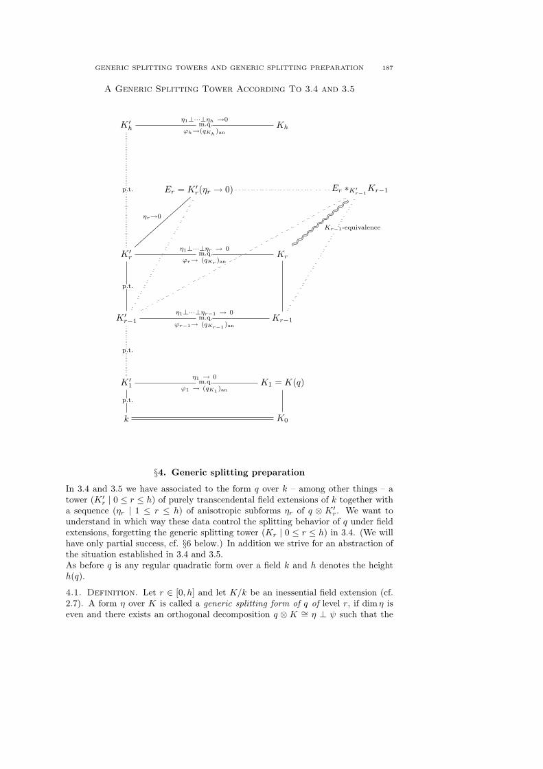
GENERIC SPLITTING TOWERS AND GENERIC SPLITTING PREPARATION 187
A Generic Splitting Tower According To 3.4 and 3.5
K ′h
m.q.η1⊥···⊥ηh →0
ϕh→(qKh)an
Kh
Er = K ′r(ηr → 0) Er ∗K′
r−1Kr−1
K ′r
m.q.η1⊥···⊥ηr → 0
ϕr→ (qKr )an
p.t.
ηr→0
|||||||||||||||||Kr
Kr−1-equivalence
<|<|
<|<|
<|<|
<|<|
<|<|
<|
<|<|
<|<|
<|<|
<|<|
<|<|
<|
K ′r−1
m.q.η1⊥···⊥ηr−1 → 0
ϕr−1→ (qKr−1 )an
p.t.
Kr−1
K ′1
m.q.ϕ1 → (qK1 )an
η1 → 0
p.t.
K1 = K(q)
k
p.t.
K0
§4. Generic splitting preparation
In 3.4 and 3.5 we have associated to the form q over k – among other things – atower (K ′
r | 0 ≤ r ≤ h) of purely transcendental field extensions of k together witha sequence (ηr | 1 ≤ r ≤ h) of anisotropic subforms ηr of q ⊗ K ′
r. We want tounderstand in which way these data control the splitting behavior of q under fieldextensions, forgetting the generic splitting tower (Kr | 0 ≤ r ≤ h) in 3.4. (We willhave only partial success, cf. §6 below.) In addition we strive for an abstraction ofthe situation established in 3.4 and 3.5.As before q is any regular quadratic form over a field k and h denotes the heighth(q).
4.1. Definition. Let r ∈ [0, h] and let K/k be an inessential field extension (cf.2.7). A form η over K is called a generic splitting form of q of level r, if dim η iseven and there exists an orthogonal decomposition q ⊗K ∼= η ⊥ ψ such that the

188 MANFRED KNEBUSCH AND ULF REHMANN
following holds: If E/K is a total generic splitting field of η, then E/k is a partialgeneric splitting field of q of level r, while ψ ⊗ E is anisotropic. We further call ψthe complement (or complementary form) of η. ¤
N.B. This property does not depend on the choice of the total generic splitting fieldof E.Generic splitting forms occur whenever a higher kernel form of q is definable overan inessential field extension of k.
4.2. Proposition. Let K/k be a partial generic splitting tower of q of level r.Assume there is given an inessential subextension K ′/k of K/k and a subform ψ ofq⊗K ′ such that ψ⊗K = ker(q⊗K). Let η denote the complement of ψ in q⊗K ′,i.e., q ⊗K ′ ∼= η ⊥ ψ. (N.B. η is uniquely determined up to isometry.) Then η is ageneric splitting form of q of level r.
Proof. dim q ≡ dim ψ mod 2. Thus dim η is even. Let E/K ′ be a total genericsplitting field of η. Then q ⊗E ∼ ψ ⊗E. Thus there exists a place λ:K → E ∪∞over k. On the other hand, η⊗K ∼ 0. Thus there exists a place µ:E → K∪∞ overK ′. Since µ is also a place over k, the fields E and K are specialization equivalentover k. We conclude that also E is a generic splitting field of q of level r. Now itis evident that dimker(q ⊗ E) = dim ψ. Thus ψ ⊗ E is anisotropic. ¤
4.3. Definition. A generic splitting preparation of q is a tower of fields (K ′r | 0 ≤
r ≤ h) together with a sequence (ηr | 0 ≤ r ≤ h) of forms ηr over K ′r such that the
following holds:(1) K ′
0 = k, and η0 is the hyperbolic part of ϕ.(2) K ′
r+1/K ′r is purely transcendental for every r, 0 ≤ r < h. 6)
(3) There exist orthogonal decompositions
q ∼= η0 ⊥ ϕ0, ϕr ⊗K ′r+1
∼= ηr+1 ⊥ ϕr+1, (0 ≤ r < h).
(4) For every r ∈ [0, h] the formr|
j=0
ηj ⊗K ′r is a generic splitting form of q of
level r. ¤
The forms ϕr (0 ≤ r ≤ h) are uniquely determined (up to isometry, as always)by condition (3). We call ϕr the r-th residual form and ηr the r-th splitting formof the given generic splitting preparation. Clearly ir: = dim ηr/2 is the r-th higherindex (cf. 1.1) of q, and dim ϕh ≤ 1. If q is anisotropic then we sometimes denotethe generic splitting preparation by (K ′
r | 0 ≤ r ≤ h), (ηr | 1 ≤ r ≤ h), omittingthe trivial form η0 = 0. ¤
4.4. Scholium. Generic splitting preparations of q exist in abundance. Indeed, inthe situation described in 3.4 and 3.5, the tower of fields (K ′
r | 0 ≤ r ≤ h) togetherwith the sequence (ηr | 0 ≤ r ≤ h) of forms ηr over K ′
r, where ηr for r ≥ 1 hasbeen introduced in 3.5 and η0 denotes the hyperbolic part of q, is a generic splittingpreparation of q.
6) Things below would not change much if we merely demanded that the exten-sions K ′
r+1/K ′r are inessential.

GENERIC SPLITTING TOWERS AND GENERIC SPLITTING PREPARATION 189
Proof. Let r ∈ [1, h] be fixed and εr: =r|
j=0
ηj ⊗K ′r. Then q ⊗K ′
r∼= εr ⊥ ϕr and
ker(ϕ⊗Kr) = ϕr ⊗Kr. Proposition 4.2 tells us that εr is a generic splitting formof q of level r. ¤
Notice that in this argument property (4) of Theorem 3.4 has not been used.
In the following, we study a fixed generic splitting preparation (K ′r | 0 ≤ r ≤ h),
(0 ≤ ηr ≤ h) of q with associated residual forms ϕr (0 ≤ r ≤ h). For every
r ∈ 1, . . . , h let εr denote the formr|
j=0
ηj ⊗ K ′r. We do not assume that the
preparation arises in the way described in the scholium.Our next goal is to derive a generic splitting preparation of q ⊗ L from these datafor a given field extension L/k.
4.5. Lemma. Assume that K/k is an inessential field extension. Let η be a formover K which is a generic splitting form of q, and let ψ be the complementary form,ϕ ⊗K ∼= η ⊥ ψ. Let E/K be a regular total generic splitting field of η (cf. 2.2).Finally, let K · L = K ·k L denote the free field composite of K and L over k, andE ·L = E ·k L the composite of E and L as explained in 2.2. Assume that ψ⊗E ·Lremains anisotropic. Then K · L/L is again inessential and η ⊗K · L is a genericsplitting form of q ⊗ L with complementary form ψ ⊗K · L.
Proof. Any place α: K → L ∪∞ over k extends to a place from L ·K to L overL. Thus K ·L/L is inessential. By Proposition 2.6 the field E ·k L = E ·K (K ·k L)is a total generic splitting field of η ⊗K ·L and also a partial generic splitting fieldof ϕ⊗ L. Now the claim is obvious from Definition 4.1. ¤
As in §1 and §2 we enumerate the splitting pattern SP(q) = jr | 0 ≤ r ≤ h by
0 ≤ j0 < j1 < · · · < jh = [dim q
2]
and write SP(q ⊗ L) = jr | r ∈ J with J = t(s) | 0 ≤ s ≤ e,0 ≤ t(0) < t(1) < · · · < t(e) = h.
We have e = h(q ⊗ L).
4.6. Proposition. For 0 < s ≤ e we define L′s = L ·K ′t(s) as the free composite
of the fields L and K ′t(s) over k, and we put
ζs: = ηt(s−1)+1 ⊗ L′s ⊥ · · · ⊥ ηt(s)−1 ⊗ L′s ⊥ ηt(s).
We further define L′0 = L and ζ0 as the hyperbolic part of ϕ ⊗ L. Then (L′s | 0 ≤s ≤ e), (ζs | 0 ≤ s ≤ e) is a generic splitting preparation of q ⊗ L.
Proof. For every r with 0 < r ≤ h we choose a regular total generic splitting fieldFr/K ′
r of the form εr.∗) 7) Then Fr/k is a partial generic splitting field of q of levelr. Let L · Fr = L ·k Fr denote the composite of L with Fr over k as explained in
7) The fields Fi from 1.3 will not be used in the following.
190 MANFRED KNEBUSCH AND ULF REHMANN
2.2. If 0 < s ≤ e, then the field L · Ft(s) is a generic splitting field of ϕ ⊗ L andker(ϕ⊗ L · Ft(s)) = ϕt(s) ⊗ L · Ft(s) by Proposition 2.6. We have
ϕ⊗ L′s ∼= εt(s) ⊗ L′s ⊥ ϕt(s) ⊗ L′s.
Again by 2.6, the field
L ·k Ft(s) = (L ·k K ′t(s)) ·K′
t(s)Ft(s) = L′s ·K′
t(s)Ft(s)
is a total generic splitting field of εt(s)⊗L′s. The form ϕt(s)⊗L′s remains anisotropicover L ·k Ft(s). Now Proposition 4.2 tells us that εt(s) ⊗ L′s is a generic splittingform of ϕ⊗ L′s, and we are done. ¤
4.7. Corollary. Let m ∈ [1, h] be fixed, and let F be a regular total genericsplitting field of εm. For every r with m < r ≤ h let F ·K ′
r denote the free compositeof F and K ′
r over k. Then the tower F ⊂ F ·K ′m+1 ⊂ · · · ⊂ F ·K ′
h together withthe sequence (ηr ⊗ F · K ′
r | m < r ≤ h) is a generic splitting preparation of theanisotropic form ϕm ⊗ F .
Proof. We apply Proposition 4.6 with L = F . Now J = m,m + 1, . . . h. Thuse = h−m and t(s) = s+m (0 ≤ s ≤ h−m). The form q⊗F has the kernel formϕm ⊗ F . ¤
We now look for generic splitting preparations with K ′1 = · · · = K ′
h. These are the“generic decompositions” according to the following definition.
4.8. Definition. Let K ′ ⊃ k be a purely transcendental field extension. A genericsplitting decomposition of q over K ′ is a sequence (α0, α1, . . . , αh) of forms over K ′
of even dimensions such that the following holds.i) q ⊗K ′ ∼= α0 ⊥ α1 ⊥ · · · ⊥ αh ⊥ ϕh with dimϕh ≤ 1.ii) α0 is the hyperbolic part of q ⊗K ′. For every r with 1 ≤ r ≤ h the form
α0 ⊥ · · · ⊥ αr is a generic splitting form of q of level r. ¤The next proposition tells us that we can always pass from a generic splittingpreparation of q to a generic splitting decomposition of q.
4.9. Proposition. As before, let (K ′r | 0 ≤ r ≤ h), (ηr | 0 ≤ r ≤ h) be a
generic splitting preparation of q. Then (ηr ⊗K ′h | 0 ≤ r ≤ h) is a generic splitting
decomposition of q over K ′h.
Proof. Let K ′: = K ′h and αr: = ηr ⊗K ′
h (0 ≤ r ≤ h). Since η0 is the hyperbolicpart of q and K ′/k is purely transcendental, the form α′0 is the hyperbolic partof q ⊗ K ′. For 1 ≤ r ≤ h we have – with the notations from above – εr ⊗ K ′ =α0 ⊥ · · · ⊥ αr. Let Fr be a regular total generic splitting field of εr (over K ′
r),hence a partial generic splitting field of q (over k) of level r. The free compositeFr ·K ′ = Fr ·K′
rK ′ is a total generic splitting field of εr ⊗K ′ = αr by Proposition
2.6. Now Fr · K ′ is purely transcendental over Fr. Thus Fr · K ′ is also a partialgeneric splitting field of q of level r. We have q ⊗K ′ ∼= αr ⊥ (ϕr ⊗K ′). The formϕr ⊗ Fr is anisotropic. Since Fr · K ′/Fr is purely transcendental, it follows that(ϕr⊗K ′)⊗Fr ·K ′ = (ϕr⊗Fr)⊗Fr ·K ′ is anisotropic. Thus αr is a generic splittingform of q of level r. ¤
Although generic splitting decompositions look simpler than generic splitting prepa-rations, it is up to now not clear to us which of the two concepts is better to workwith. See also our discussion below at the end of §6.
GENERIC SPLITTING TOWERS AND GENERIC SPLITTING PREPARATION 191
§5. A brief look at quadratic places
We need some more terminology.If K is a field, we denote the group of square classes K∗/K∗2 by Q(K) and a singlesquare class aK∗2 by 〈a〉, identifying this class with the bilinear form 〈a〉 over K.If λ:K → L ∪ ∞ is a place with associated valuation ring o = oλ, we denote theimage of the unit group o∗ in Q(K) by Q(o). Notice that Q(o) ∼= o∗/o∗2, and thatλ gives us a homomorphism λ∗: Q(o) → Q(L), λ∗(〈ε〉) = 〈λ(ε)〉. (The bilinearform 〈ε〉 has good reduction under λ and λ∗(〈ε〉) is the specialization of this formunder λ.)
5.1. Definition. A quadratic place, or Q-place for short, from a field K to a fieldL is a triple (λ,H, χ) consisting of a place λ: K → L ∪∞, a subgroup H of Q(K)containing Q(oλ), and a homomorphism χ: H → Q(L) (called a “character” in thefollowing) extending the homomorphism λ∗: Q(oλ) → Q(L). ¤We often denote such a triple (λ,H, χ) by a capital Greek letter Λ and symbolicallywrite Λ: K → L ∪∞ for the Q-place Λ.Every place λ: K → L ∪ ∞ gives us a Q-place λ = (λ, Q(oλ), λ∗): K → L ∪ ∞,where λ∗: Q(oλ) → Q(L) is defined as above. We regard λ and λ essentially as thesame object. In this sense Q-places are a generalization of the usual places.
5.2. Definition. If Λ = (λ,H, χ): K → L ∪∞ is a Q-place then an expansion ofΛ is a Q-place Λ′ = (λ,H ′, χ′): K → L ∪∞ with the same first component λ as Λ,a subgroup H ′ of Q(K) containing H, and a character χ′: H ′ → Q(L) extendingχ. ¤Usually Λ allows many expansions, and Λ itself is an expansion of λ.In the following Λ = (λ,H, χ): K → L ∪∞ a Q-place and o: = oλ.
5.3. Definitions. Let k be a subfield of K.a) The restriction Λ|k of the Q-place Λ to k is the Q-place (ρ,E, σ) where
ρ = λ|k: k → L∪∞ denotes the restriction of the place λ:K → L∪∞ in theusual sense, E denotes the preimage of H in Q(k) under the natural mapj: Q(k) → Q(K), and σ denotes the character χ (j|D) from D to Q(L).
b) If Γ: k → L ∪∞ is any Q-place from k to L then we say that Λ extends Γ(or, that Λ is an extension of Γ), if Λ|k is an expansion of Γ. ¤
At the first glance one might think that this notion of extension is not strongenough. One should demand Λ|k = Γ, in which case we say that Λ is a strictextension of Γ. But it will become clear below (cf. 5.8.ii, 5.12, 6.1) that the weakernotion of extension as above is the one needed most often.As before, we stay with a Q-place Λ = (λ,H, χ): K → L ∪∞.
5.4. Definition. Let ϕ be a regular quadratic form over K. We say that ϕ hasgood reduction (abbreviated: GR) under Λ, if there exists an orthogonal decompo-sition
(∗) ϕ = |h∈H
hψh
with forms ψh over K which all have GR under λ. Here hψh denotes the product〈h〉 ⊗ ψh of the bilinear form 〈h〉 with ψh. This amounts to scaling ψh by arepresentative of the square class 〈h〉. Of course, ψh 6= 0 for only finitely manyh ∈ H.

192 MANFRED KNEBUSCH AND ULF REHMANN
Alternatively we say in this situation that ϕ is Λ-unimodular. In harmony withthis speaking we call a form ψ over K, which has GR under λ, also a λ-unimodularform. ¤5.5. Remark. We may choose a subgroup U of H such that H = U ×Q(o). If ϕhas GR under Λ then we can simplify the decomposition (∗) to a decomposition
ϕ ∼= |u∈U
uϕu
with λ-unimodular forms ϕu. ¤5.6. Proposition. If ϕ has GR under Λ, and a decomposition (∗) is given, thenthe form |
h∈H
χ(h)λ∗(ψh) is up to isometry independent of the choice of the decom-
position (∗).This has been proved in [K4] if charL 6= 2. A proof in general (which is ratherdifferent) will be contained in [K5].
5.7. Definition. If ϕ has GR under Λ then we denote the form |h∈H
χ(h)λ∗(ψh)
(cf. 5.6) by Λ∗(ϕ), and we call Λ∗(ϕ) the specialization of ϕ under λ. ¤5.8. Remarks.
i) If ψ is a second form over K such that ϕ ⊥ ψ is regular, and if both ϕ andψ have GR under Λ then ϕ ⊥ ψ has GR under Λ and
Λ∗(ϕ ⊥ ψ) ∼= Λ∗(ϕ) ⊥ Λ∗(ψ).
ii) Assume that k is a subfield of K and Γ: k → L ∪∞ is a Q-place such thatΛ extends Γ (cf.5.3.b). Let q be a regular form over k which has GR underΓ. Then q ⊗K has GR under Λ and Λ∗(q ⊗K) ∼= Γ∗(q).
We omit the easy proofs. ¤It seems that quadratic places come up in connection with generic splitting forms(cf. 4.1) in a natural way. We illustrate this by a little proposition, which will alsoserve us to indicate some of the difficulties we have to face if we want to make gooduse of quadratic places in generic splitting business.
5.9. Proposition. Let q be an anisotropic regular form over a field k, dim q > 2.Let k(q) denote the function field of the projective quadric q = 0. Let L ⊃ kbe a field extension such that qL = q ⊗ L is isotropic. Then there is a purelytranscendental subextension k′/k of k(q)/k, such that k(q)/k′ is separable quadratic,and a quadratic place Λ: k′ → L ∪∞ over k, such that the form α described in 3.3qk′ ∼= α ⊥ q′, αk(q) ∼ 0, q′k(q) anisotropic has GR under Λ and Λ∗(α) ∼ 0.
Proof. Since qL is isotropic we have a place λ: k(q) → L∪∞ over k. Let o denotethe valuation ring of λ, let V denote the underlying k-vector space of q. We take a
decomposition V ∼=r
|i=1
(kei ⊕ kfi) ⊥ V ′ with kei ⊕ kfi = [ai, bi], and V ′ = 〈a0〉 or
V ′ = 0, and ai, bi, a0 ∈ k∗.We choose a primitive isotropic vector x ∈ Vo = o ⊗k V with (x, Vo) = o. Byrearranging coordinates over k we may assume that x = Xe1 + Y f1 + z, and
X ∈ o \ 0, Y ∈ o∗, z ∈r
|i=2
(oei ⊕ kofi) ⊥ oV ′, and after dividing by Y , we

GENERIC SPLITTING TOWERS AND GENERIC SPLITTING PREPARATION 193
may assume that Y = 1. We take the coordinates ofr
|i=2
(oei ⊕ ofi) ⊥ oV ′ as
independent variables over k, which generate a purely transcendental subfield k′ ofk(q). The equation 0 = qo(x) = a1X
2 +X + b with b = b1 + qk(q)(z) ∈ o∩k′ definesthe field k(q) as a separable quadratic extension of k′.By construction we have λ(b) 6= ∞. Hence the quadratic form [a1, b] has goodreduction under this place. We write α = [a1, b] ⊗ 〈c1, . . . , ci〉 with cν ∈ =(qk′) \ 0according to 3.2. We denote the restriction of λ to k′ by λ′, and the associatedvaluation ring by o′(= o ∩ k′).Let H denote the subgroup of Q(k′) which is generated by Q(o′) and the classes〈c1〉, . . . , 〈ci〉. We choose some extension χ:H → Q(L) of the character λ′∗: Q(o′) →Q(L). The quadratic place Λ = (λ′,H, χ) has the desired properties. Alternativelywe may choose for Λ the restriction of λ to k′. ¤
This proposition leaves at least two things to be desired. Firstly, it would be niceand much more useful, to have the subextension k′/k to be chosen in advance,independently of the place λ in the proof. Secondly it would be pleasant if alsothe form q′ has GR under Λ. This is by no means guaranteed by our proof. Wesee no reason, why the analogue of Lemma 1.15.b for quadratic places instead ofordinary places should be true. The main crux here is the case char k = 2. Thenusually many forms over k′ do not admit λ′-modular decompositions for a givenplace λ′: k′ → L ∪ ∞ over k. It is easy to give counterexamples in a sufficientlygeneral situation, cf. [K5]. On the other hand, if we can achieve in Proposition5.9 in addition that q′ has GR under Λ, then the equation
q ⊗ L = Λ∗(α) ⊥ Λ∗(q′),
which follows from the remarks 5.8 above, together with Λ∗(α) ∼ 0 would “explain”that q⊗L is isotropic, and how the anisotropic part of q⊗L is connected with thegeneric splitting form α of q of level 1.If char k 6= 2 it is still not evident that the analogue of 1.15.b holds for the quadraticplace Λ′ but now at least every form over k′ has a λ′-modular decomposition.Indeed, this trivially holds for forms of dimension 1, hence for all forms. In [K4] away has been found, to force an analogue of 1.15.b for quadratic places to be true,by relaxing the notion “good reduction” to a slightly weaker – but still useful –notion “almost good reduction”.We can define “almost good reduction” without restriction to characteristic 6= 2 asfollows.
5.10. Definition. Let Λ = (λ,H, χ): K → L ∪∞ be a Q-place, o: = oλ, and letS be a subgroup of Q(K) such that Q(K) = S ×H. A form ϕ over K has almostgood reduction (abbreviated AGR) under Λ if ϕ has a decomposition
(∗∗) ϕ ∼= |s∈S
sϕs
with Λ-unimodular forms ϕs and Λ∗(ϕs) ∼ 0 for every s ∈ S, s 6= 1. In this casewe call the form
Λ∗(ϕ):= Λ∗(ϕ1) ⊥ (dimϕ− dim ϕ1)/2×H
the specialization of ϕ under Λ. ¤
194 MANFRED KNEBUSCH AND ULF REHMANN
The point here is that Λ∗(ϕ) is independent of the choice of the decomposition (∗∗)and also of the choice of S. This has been proved in [K4] in the case char L 6= 2.It also holds if char L = 2, cf. [K5].It now is almost trivial that the analogue of 1.15. holds for Q-places with AGRinstead of GR, provided char L 6= 2, cf. [K4, §2].
5.11. Proposition. Let Λ: K → L ∪∞ be a Q-place and let ϕ and ψ be regularforms over K. Assume that char L 6= 2.
a) If ϕ and ψ have AGR under Λ, then ϕ ⊥ ψ has AGR under Λ and
Λ∗(ϕ ⊥ ψ) ∼= Λ∗(ϕ) ⊥ Λ∗(ψ).
b) If ϕ and ϕ ⊥ ψ have AGR under Λ, then ψ has AGR under Λ. ¤5.12. Proposition. Let k ⊂ K be a field extension. Let Γ: k → L ∪ ∞ andΛ:K → L ∪ ∞ be Q-places with Λ extending Γ. Assume finally that q is a formover k with AGR under Γ. Then q⊗K has AGR under Λ and Λ∗(q⊗K) ∼= Γ∗(q).
The proof has been given in [K4, §3] for char L 6= 2. The arguments are merelybook keeping. They remain true if char L = 2. ¤Now we can repeat the arguments in the proof of Proposition 1.16 for quadraticplaces and AGR instead of usual places and GR, provided char L 6= 2. We obtainthe following.
5.13. Proposition. Let Λ: K → L ∪∞ be a Q-place and ϕ a form over K withAGR under Λ. Assume that char L 6= 2. Then ϕ0: = ker(ϕ) has again AGR underΛ and Λ∗(ϕ) ∼ Λ∗(ϕ0), ind Λ∗(ϕ) ≥ ind (ϕ). If ind Λ∗(ϕ) = ind (ϕ), thenker Λ∗(ϕ) = Λ∗(ϕ0). ¤We finally state an important fact, proved in [K4, §3], which has no counterpart onthe level of ordinary places.
5.14. Proposition. Let again Λ:K → L∪∞ be a Q-place with char L 6= 2. Let kbe a subfield of K and Γ:= Λ|k. Let q be a regular form over k. Then q⊗L has AGRunder Λ if and only if q has AGR under Γ, and in this case Λ∗(q ⊗ L) ∼= Γ∗(q). ¤
§6. Control of the splitting behavior by use of quadratic places
If we stay with fields of characteristic 6= 2 then the propositions 5.11 – 5.13 indicatethat it should be possible to obtain a complete analogue of the generic splittingtheory displayed in §1 using quadratic places instead of ordinary places. Indeedsuch a theory has been developed in [K4, §3]. We quote here the main resultobtained there.Let q be a form over a field k. We return to some notations from §1: (Kr | 0 ≤ r ≤ h)is a generic splitting tower of q with higher indices (ir | 0 ≤ r ≤ h) and higher kernelforms (ϕr | 0 ≤ r ≤ h). Further (jr | 0 ≤ r ≤ h), with jr = i0 + · · · + ir, is thesplitting pattern SP(q) of q.
6.1. Theorem. [K4, Th. 3.7]. Let Γ: k → L ∪ ∞ be a Q-place into a field Lof characteristic 6= 2. Assume that q has AGR under Γ. We choose a Q-placeΛ:Km → L ∪ ∞ extending Γ such that either m = h or m < h and Λ does notextend to a Q-place from Km+1 to L. Then ind (Γ∗(q)) = jm, the form ϕm has GRunder Λ and ker(Γ∗(q)) ∼= Λ∗(ϕm). ¤A small point here – which we will not really need below – is that ϕm has GR underΛ, not just AGR.

GENERIC SPLITTING TOWERS AND GENERIC SPLITTING PREPARATION 195
6.2. Remark.The theorem shows that the generic splitting tower (Kr | 0 ≤ r ≤ h) “controls” thesplitting behavior of Γ∗(q). Indeed, if L′/L is any field extension then we obtainfrom Γ a Q-place j Γ: k → L′ ∪∞ in a rather obvious way (cf. 6.4.iii below). Theform q has also AGR under j Γ, and (j Γ)∗(q) = Γ∗(q)⊗ L′. We can apply thetheorem to jΓ and q instead of Γ and q. In particular we see that ind (Γ∗(q)⊗L′) isone of the numbers jr. Thus the splitting pattern SP(Γ∗(q)) is a subset of SP(q).¤We now aim at a result similar to Theorem 6.1, where the field Km is replaced byan arbitrary partial generic splitting field for q. (This is not covered by [K4].) Forthat reason we briefly discuss the “composition” of Q-places.
6.3. Definition. Let Λ = (λ,H, χ): K → L ∪∞ and M = (µ,D, ψ): L → F ∪∞be Q-places. The composition M Λ of M and Λ is the Q-place
(M Λ) = (µ λ, H0, ψ (χ|H0))
with H0: = α ∈ H | χ(α) ∈ D. ¤6.4. Remarks.
i) If N :F → E ∪∞ is a third Q-place then N (M Λ) = (N M) Λ, as iseasily checked.
ii) Let i: k → K be a field extension, regarded as a trivial place. This givesus a “trivial” Q-place i = (i, Q(k), i∗:Q(k) → Q(K)) from k to K. IfΛ = (K, H, χ): K → L ∪∞ is any Q-places starting at K, then Λ i is therestriction Λ|k: k → L ∪∞.
iii) The Q-place j Γ alluded to in 6.2 is j Γ. ¤In all the following Γ: k → L∪∞ is a Q-place into a field of characteristic 6= 2 suchthat q has AGR under Γ.
6.5. Proposition. Let F/k be a generic splitting field of the form q of some levelr ∈ [0, h]. Assume that ind Γ∗(q) ≥ jr. Then there exists a Q-place Λ:F → L ∪∞extending Γ. For any such Q-place Λ the anisotropic part ϕ = ker(q⊗F ) of q⊗F hasAGR under Λ and Λ∗(ϕ) ∼ ker Γ∗(q). if ind Γ∗(q) = jr, then Λ∗(ϕ) = ker Γ∗(q).
Proof. We only need to prove the existence of a Q-place Λ: F → L∪∞ extendingΓ. The other statements are clear from §5 (cf. 5.12, 5.13). By Theorem 6.1 wehave a Q-place Λ′: Kr → L ∪∞ extending Γ. We further have a place ρ: F → Kr
over k. It now can be checked in a straightforward way that the Q-place Λ = Λ′ ρfrom F to L extends Γ. ¤
6.6. Theorem. Let K/k be an inessential field extension and q⊗K ∼= η ⊥ ϕ withη a generic splitting form of q of some level r ∈ [0, h]. Assume that ind Γ∗(q) ≥ jr.Then there exists a Q-place Λ:K → L∪∞ extending Γ such that η has AGR underΛ and Λ∗(η) ∼ 0. For every such Q-place Λ the form ϕ has AGR under Λ andΛ∗(ϕ) ∼ Γ∗(q). If ind Γ∗(q) = jr, then Λ∗(ϕ) = ker Γ∗(q).
Proof. Again it suffices to prove the existence of a Q-place Λ extending Γ suchthat η has AGR under Λ and Λ∗(η) ∼ 0, the other statements being covered by §5(cf. 5.11, 5.12).Let E be a total generic splitting field of η. Then E is a partial generic splitting fieldof q (cf. 4.1). By the preceding proposition 6.5 there exists a Q-place M : E → L∪∞

196 MANFRED KNEBUSCH AND ULF REHMANN
extending Γ. Let Λ: K → L ∪ ∞ denote the restriction of M to K (cf. 5.3). Ofcourse, also Λ extends Γ. The form η ⊗ E is hyperbolic, hence certainly has AGRunder M and M∗(η⊗E) ∼ 0. Now Proposition 5.14 tells us that η has AGR underΛ and Λ∗(η) ∼ 0. ¤
6.7. Remark. Suppose that Γ = γ with γ: k → L ∪ ∞ a place and that q hasGR under γ. Then Theorem 6.1 and Proposition 6.5 give us nothing more than weknow from the generic splitting theory in §1. Indeed, if Λ = (λ,H, χ) is a Q-placeas stated there, then the form ϕm in 6.1, resp. ϕ in 6.5, automatically has GRunder λ.This is different with Theorem 6.6. Even in the case Γ = j for j: k → L theinclusion map into an overfield L of k (actually the case which is perhaps the mosturgent at present), the Q-place Λ will be different from λ. Thus, in 6.6, Q-placesinstead of usual places are needed even in the case Γ = j. ¤We now choose again a generic splitting preparation (K ′
r | 0 ≤ r ≤ h), (ηr | 0 ≤ r ≤h) of q with residual forms ϕr and generic splitting forms εr =
r
|j=0
ηj ⊗K ′j (0 ≤
r ≤ h), cf. 4.3.
6.8. Discussion. Assume that ind Γ∗(q) ≥ jm for some m ∈ [0, h]. Theorem 6.6tells us that there exists a Q-place Λ: K ′
m → L ∪∞ extending Γ such that εm hasAGR under Λ and Λ∗(εm) ∼ 0. Moreover, for every such Q-place λ the form ϕm
has AGR under Λ and Λ∗(ϕm) ∼ Γ∗(q). If ind Γ∗(q) = jm, it follows that Λ∗(ϕm)is the anisotropic part of Γ∗(q).Assume now that ind Γ∗(q) > jm and Λ: K ′
m → L∪∞ is a Q-place as just described.Then by analogy with 1.18 one might suspect at first glance that Λ extends to aplace M :K ′
m+1 → L ∪∞ such that εm+1 has AGR under M and M∗(εm+1) ∼ 0.N.B. Since Λ∗(εm) ∼ 0, this is equivalent to the property that ηm+1 has AGRunder M and M∗(ηm+1) ∼ 0. But this is too much to be hoped for. Indeed, letus consider the special case that K ′
1 = · · · = K ′h =:K ′, i.e., we are given a generic
splitting preparation (η0, η1, . . . , ηh) over K ′. If Λ: K ′ = K ′m → L∪∞ is as above,
then we can expand Λ = (λ,H, χ) to a Q-place Λ′ = (λ,Q(K ′), ψ′): K ′ → L ∪∞.Also Λ′ extends Γ, further εm has AGR under Λ′ and Λ′∗(εm) = Λ∗(εm) ∼ 0 (cf.5.12). But since K ′
m+1 = K ′, the only extension of Λ′ to K ′m+1 is Λ′ itself, and
there is no reason why ηm+1 should have AGR under Λ′ and Λ′∗(ηm+1) ∼ 0. ¤Nevertheless, if ind Γ∗(q) > jm+1, there exists a somewhat natural procedure toobtain from a Q-place Λ: K ′
m → L ∪ ∞ as above a Q-place M : K ′m+1 → L ∪ ∞
extending Γ such that both εm⊗K ′m+1 and εm+1 have AGR under M and we have
M∗(εm ⊗K ′m+1) ∼ 0 as well as M∗(εm+1) ∼ 0. This runs as follows.
6.9. Procedure. Assume that ind Γ∗(q) > jm. Let Λ: K ′m → L∪∞ be a Q-place
extending Γ such that εm has AGR under Λ and Λ∗(εm) ∼ 0. We choose a regulartotal generic splitting field F of εm. By Proposition 6.5 the Q-place Λ extends to aQ-place Λ:F → L∪∞. The form ϕm⊗F is anisotropic. We now invoke Corollary4.7, which tells us that the tower F ⊂ F ·K ′
m+1 ⊂ · · · ⊂ F ·K ′h together with the
sequence of forms (ηr ⊗ F · K ′r | m < r ≤ h) is a generic splitting preparation of
ϕm ⊗ F . Here F · K ′r denotes the free composite of the fields F and K ′
r over k.In particular ηm+1 ⊗ F · K ′
r is a generic splitting form of ϕm ⊗ F over F · K ′r of
level 1. We have Λ∗(ϕm ⊗ F ) ∼ Λ∗(q ⊗ F ) = Γ∗(q). Since ind Γ∗(q) > jm, we

GENERIC SPLITTING TOWERS AND GENERIC SPLITTING PREPARATION 197
conclude that Λ∗(ϕm ⊗ F ) is isotropic. Thus, again by Proposition 6.5, Λ extendsto a Q-place M : F ·K ′
m+1 → L∪∞ such that ηm+1⊗F ·K ′m+1 has AGR under M
and M∗(ηm+1 ⊗ F ·K ′m+1) ∼ 0. Let M : K ′
m+1 → L ∪∞ denote the restriction ofM to K ′
m+1. By 5.14, the form ηm+1 has AGR under M and M∗(ηm+1) ∼ 0.Now we need a delicate argument to prove that also εm ⊗K ′
m+1 has AGR underM and M∗(εm⊗K ′
m+1) ∼ 0. The problem is that the diagram of field embeddings
F // F ·K ′m+1
K ′m
OO
// K ′m+1
OO
does not commute, since the field composite F · K ′m+1 is built over k instead of
K ′m. Thus M probably does not extend the Q-place Λ.
The argument runs as follows. Also ϕm+1 ⊗ F ·K ′m+1 has AGR under M , hence
ϕm+1 has AGR under M , and
M∗(ϕm+1) ∼= M∗(ϕm+1 ⊗ F ·K ′m+1) ∼ Λ∗(ϕm ⊗ F ) ∼ Λ∗(q ⊗ F ) ∼= Γ∗(q).
Since q ⊗K ′m+1
∼= εm ⊗K ′m+1 ⊥ ηm+1 ⊥ ϕm+1 and both, ηm+1 and ϕm+1, have
AGR under M , also εm ⊗K ′m+1 has AGR under M , cf. 5.11, and
Γ∗(q) ∼= M∗(q ⊗K ′m+1) ∼= M∗(εm ⊗K ′
m+1) ⊥ M∗(ηm+1) ⊥ M∗(ϕm+1).
Since M∗(ηm+1) ∼ 0 and M∗(ϕm+1) ∼ Γ∗(q), we conclude that M∗(εm ⊗ K ′m+1)
∼ 0. ¤
We have ind Γ∗(q) = jr for some r ∈ [0, h] (cf. 6.2). Iterating the procedure withm = 0, 1, . . . , r − 1, we obtain the following theorem.
6.10. Theorem. Let ind Γ∗(q) = jr. Then there exists a Q-place Λ:K ′r → L∪∞
extending Γ such that ηm ⊗K ′r has AGR under Λ and Λ∗(ηm ⊗K ′
r) ∼ 0 for everym ∈ [0, r]. If Λ is any such Q-place then ϕr has AGR under Λ and Λ∗(ϕr) =ker Γ∗(q).
We briefly discuss the case that L is a field extension of k and Γ = j with j: k → Lthe inclusion map.
6.11. Definition/Remark. Let K and L be field extensions of k. A Q-place fromK to L over k is a Q-place Λ = (λ,H, χ): K → L∪∞ such that the first componentλ is a place over k. It is evident from Definitions 5.3 that this condition just meansthat Λ extends the quadratic place j: k → L ∪∞, and also that Λ|k = j. ¤
6.12. Scholium. Let L/k be a field extension, ind (q ⊗ L) = jr. Then thereexists a Q-place Λ:K ′
r → L ∪∞ over k such that ηm ⊗K ′r has AGR under Λ and
Λ∗(ηm ⊗ K ′r) ∼ 0 for every m ∈ [0, r]. For any such Q-place Λ the form ϕr has
AGR under Λ and Λ∗(ϕr) = ker(q ⊗ L). ¤
We return to an arbitrary Q-place Γ: k → L ∪∞ such that q has AGR under Γ.
6.13. Definition. We call the generic splitting preparation (K ′r | 0 ≤ r ≤ h),
(ηr | 0 ≤ r ≤ h) of q tame, if there exists a generic splitting tower (Kr | 0 ≤ r ≤ h)of q such that K ′
r is a subfield of Kr and ηr ⊗Kr ∼ 0 for every r ∈ [0, h]. ¤
198 MANFRED KNEBUSCH AND ULF REHMANN
Notice that a generic splitting preparation (K ′r | 0 ≤ r ≤ h), (ηr | 0 ≤ r ≤ h)
as described by 3.4 and 3.5 is tame. Thus every form admits tame generic split-ting preparations. On the other hand we suspect that there exist generic splittingpreparations which are wild (= not tame), although we did not look for examples.If our given generic splitting preparation of q is tame then there exists a muchsimpler procedure than the one described above, to obtain a Q-place Λ: K ′
r → L∪∞with the properties stated in Theorem 6.10.
6.14. Procedure. Assume that ind Γ∗(q) = jr, and that (Ki | 0 ≤ i ≤ h) is ageneric splitting tower of q such that K ′
i is a subfield of Ki and εi ⊗ Ki ∼ 0 forevery i ∈ [0, h]. By 6.1 there exists a Q-place Λ:Kr → L ∪ ∞ extending Γ. LetΛ denote the restriction of Λ to K ′
r. Then Λ again extends Γ. For every i ∈ [0, r]we have (εi ⊗K ′
r) ⊗Kr = εi ⊗Kr ∼ 0. Certainly εi ⊗Kr has AGR under Λ andΛ∗(εi⊗Kr) ∼ 0. By 5.14 the form εi⊗K ′
r has AGR under Λ and Λ∗(εi⊗K ′r) ∼ 0.
Since this holds for every i ∈ [0, r] we conclude (using 5.11) that ηi ⊗K ′r has AGR
under Λ and Λ∗(ηi ⊗K ′r) ∼ 0 for every i ∈ [0, r].
Thus it seems that life is easier if we have a tame generic splitting preparationat our disposal than an arbitrary one. Up to now this is an argument in favorof working with generic splitting preparations instead of the more special genericsplitting decompositions (cf. 4.8), in spite of Proposition 4.9, for we do not knowwhether every form admits a tame generic splitting decomposition.
References
[A] C. Arf, Untersuchungen uber quadratische Formen in Korpern der Charak-teristik 2 (Teil I). J. reine angew. Math. 183 (1941), 148–167.
[HR1] J. Hurrelbrink and U. Rehmann, Splitting patterns of excellent quadraticforms, J. reine angew. Math. 444 (1993), 183–192.
[HR2] J. Hurrelbrink and U. Rehmann, Splitting patterns and linear combinationsof two Pfister forms. J. reine angew. Math. 495 (1998), 163–174
[J] N. Jacobson, “Lectures in abstract algebra” III, Theory of fields and Galoistheory, New York, Heidelberg, Berlin: Springer 1964.
[KR] I. Kersten and U. Rehmann, Generic splitting of reductive groups, TohokuMath. J. 46 (1994), 35–70.
[K1] M. Knebusch, Specialization of quadratic forms and symmetric bilinearforms, and a norm theorem, Acta Arithmetica, 24 (1973), 279–299.
[K2] M. Knebusch, Generic splitting of quadratic forms, I, Proc. London Math.Soc. 33 (1976), 65–93.
[K3] M. Knebusch, Generic splitting of quadratic forms, II, Proc. London Math.Soc. 34 (1977), 1–31.
[K4] M. Knebusch, Generic splitting of quadratic forms in the presence of badreduction, J. reine angew. Math. 517 (1999), 117–130.
[K5] M. Knebusch, “Spezialisierung von quadratischen und symmetrischen bilin-earen Formen”, Book in preparation.
[Lg] S. Lang, “Introduction to algebraic geometry”. New York: Interscience 1958.[W] E. Witt, Theorie der quadratischen Formen in beliebigen Koerpern. J. reine
angew. Math. 176 (1937), 31–44.

GENERIC SPLITTING TOWERS AND GENERIC SPLITTING PREPARATION 199
Fachbereich MathematikUniversitat RegensburgD93040 RegensburgGermanyE-mail address: [email protected]
Fakultat fur MathematikUniversitat BielefeldD33501 BielefeldGermanyE-mail address: [email protected]

Contemporary MathematicsVolume 00, 2000
Local densities of hermitian forms
Maurice Mischler
Abstract. Local densities are used in the calculation of mass formulae. Theaim of this paper is to describe how to compute the local density of a givenhermitian form, knowing its usual invariants such as the Jordan decompositionor invariant factors. Note that explicit formulae have been already obtainedby Y. Hironaka in [5] and [6] but only in the case of inert primes.
1. Introduction
Let E be a totally complex number field with complex multiplication, and Kthe fixed field under complex conjugation. Let B be the ring of integers of E, andA be the ring of integers of K.
We say that (M, h) is a hermitian B-lattice if M is a projective module of finiterank over B equipped with a nondegenerate hermitian form h, the involution beingdefined by complex conjugation. Two hermitian B-lattices (M, h) and (N, k) aresaid to be in the same genus if
Mp := (M,h)⊗B (B ⊗A Ap) is isometric to (N, k)⊗B (B ⊗A Ap) =: Np
for every spot p of K and where Ap is the completion of A at p. We suppose that(M, h) is totally definite. This means that h is positive at every infinite spot. Thefollowing theorem gives an example of the application of local densities when E isa cyclotomic field.
Theorem 1.1. Suppose that E = Q(ζd) is a cyclotomic field. Let (M, h) be atotally definite hermitian B-lattice of rank n. Denote by GM the genus of M (up toisometry). The mass of GM is the following sum:
ω(M, h) :=∑
L∈GM
1|U(L)|
Key words and phrases. Local densities, mass of hermitian forms.The author thanks the referee for interesting remarks, Prof.J. Boechat for fruitful discussions
and the organizers of the conference for the opportunity to give a talk.2000 Mathematics Subject Classification: 11E39.
c©2000 American Mathematical Society
201

202 MAURICE MISCHLER
where |U(L)| is the cardinality of the unitary group of any representative of theclass L. Then we have
ω(M, h) = 2 · |d(E)|n(n+1)4 · |d(K)|−n
2 ·
n∏
j=1
(j − 1)!(2π)j
ϕ(d)2
·det(M)n2 ·
∏
p∈PBp(Mp)−1
where det(M) = [M# : M ] with M# = x ∈ M ⊗ E | h(x,M) ⊂ B, d(E) andd(K) are the discriminants of the fields E and K respectively, P is the set of allfinite spots of K and Bp(Mp) is the local density of Mp.
We will give the precise definition of local density in the next part.The proof of this theorem is very long and technical. See ([9], formula (4.5),
p. 20), ([2], p. 112]), and ([3], Satz VI). For more general formulae, see the won-derful book of Shimura [11]. The usefulness of this theorem is evident (for classifi-cations for instance), so we have to be able to precisely compute local densities.
2. Definitions
Let E,K, B, A be as in the introduction and p a finite spot of K. Suppose that2 6∈ p. Three cases are possible:
pB =
P inert caseP2 ramified caseP1 ·P2 decomposed case
for some prime ideals P, P1,P2 of B. Write R = B ⊗A Ap. The classical theory oflocalisation shows that
R =
BP in the inert and ramified caseBP1 ×BP2 ' Ap ×Ap in the decomposed case.
Finally, if π is a uniformizing parameter of Ap such that pAp = πAp, we can supposethat
pR =
p ·R in the inert case, with p = π
p 2 ·R in the ramified case, with p 2 = π
p ·R ' πAp × πAp in the decomposed case, with p = (π, π).
In any case, let P denote the ideal p ·R.
Definition 2.1. Let (M, h) be a hermitian R-lattice. Suppose that p doesnot decompose. A vector x of M is said to be primitive if there exists an R-basis (x1, . . . , xn) of M such that x = x1. Let a be an ideal of R. We say that(M, h) is a-modular if h(x, M) = a for every primitive vector of M . If there existsm1 < · · · < ml such that the following orthogonal sum holds:
M = M1 ¢ · · ·¢ Ml
where Mi is Pmi-modular for every i, we say that M1 ¢ · · · ¢ Ml is a Jordandecomposition of (M, h). It is possible to prove that Jordan decomposition existsand that l, dim(Mi), and mi do not depend on the decomposition. In this case,Pm1 ⊃ · · · ⊃ Pml are called the invariant factors of (M, h). (See ([4], p. 33) and([7], p. 449) for proofs.)

LOCAL DENSITIES OF HERMITIAN FORMS 203
Definition 2.2. Let (M, h) be a hermitian R-lattice. Suppose that p decom-poses. There exist x1, . . . , xn ∈ M such that
M = (Ap × πm1Ap)x1 ⊕ · · · ⊕ (Ap × πmnAp)xn
and such that h(xi, xj) = δij · (1, 1) for all 1 ≤ i, j ≤ n and m1 ≤ · · · ≤ mn. In thiscase
πm1Ap ⊃ · · · ⊃ πmnAp
are called the invariant factors of (M,h), because
M# = (π−m1Ap ×Ap)x1 ⊕ · · · ⊕ (π−mnAp ×Ap)xn.
(See ([4], p. 25) or ([10], Proposition 3.2) for proofs.) In addition, (M, h) is saidto be Pm-modular if
m1 = · · · = mn = m.
Definition 2.3. Let (M,h) and (N, k) be two hermitian R-lattices of rankr ≥ s respectively. Let m ∈ N. We define Apm(M, N) to be the set of R-linearmaps u : N → M which are distinct modulo pmRM and satisfy
h(u(x), u(y)) ≡ k(x, y) (mod pmR) for all x, y ∈ N.
We write Apm(M,N) the cardinality of Apm(M, N).
Proposition 2.4. Let (M, h) and (N, k) be two hermitian R-lattices of rankr ≥ s respectively. Suppose that p ∩ Z = pZ and write q = pf = |A/p|. Then wehave:
Apm+1(M, N) = qs(2r−s)Apm(M, N)
for any m ≥ 2 · vp(al) + 1. Here a1 ⊃ · · · ⊃ al are the invariant factors of (N, k),and vp is the discrete valuation over Ap.
Proof. See ([9], Hilfssatz 5.3) for the proof. ¤
Definition 2.5 (definition of local densities). Let (M,h) be a hermit-ian R-lattice of rank r. We write
Bp(M) = limm→∞
q−r2mApm(M, M).
The last proposition shows that this limit exists. This limit is called the localdensity of (M,h).
Now, the natural question is the following: if we know the invariant factors ofa given hermitian R-lattice, is it possible to calculate its local density ? We willshow that the answer is yes!

204 MAURICE MISCHLER
3. Results
Let E, K, B, A, p, R, p, and q be as in the last part.
Proposition 3.1. Let (M, h) be a hermitian R-lattice of rank n.(a) Suppose that p does not decompose. If h = πmh′ with M ⊂ M#
h′ and m ≥1, write M ′ for (M,h′). Let l be a strictly positive integer . Then we haveApl+m(M, M) = q2mn2
Apl(M ′,M ′). This implies that
Bp(M) = qmn2Bp(M ′).
(b) Suppose that p decomposes. We have seen that we can suppose that M =(Ap×πm1Ap)x1⊕· · ·⊕ (Ap×πmnAp)xn with h(xi, xj) = δij · (1, 1). Now defineh′ such that h′(xi, xj) = (1, π−m1)h(xi, xj) for all 1 ≤ i, j ≤ n. Then we havethe same results with m1 instead of m.
Proof. In each case, let
Ψ : Apm+l(M, M) −→ Apl(M ′, M ′)
u (mod pl+mR) 7−→ u (mod plR)
The function Ψ is surjective. More precisely, if u ∈ Apl(M ′,M ′), it is easy to verifythat the set of u + πlv, where v is any endomorphism modulo pmR, is the set of u′
such that Ψ(u′) = u. Since |R/pmR| = |Ap/pm|2 = q2m, the number of v which isthe number of u′ is equal to q2mn2
. Hence Apl+m(M, M) = q2mn2Apl(M ′,M ′). So
we have proved the proposition. Indeed, for l big enough, we have:
Bp(M) =Apl+m(M,M)
q(l+m)n2 =q2mn2
Apl(M ′,M ′)qmn2qln2 = qmn2
Bp(M ′). ¤
Proposition 3.2. Let (M, h) be a hermitian R-lattice of rank n. Suppose that(M, h) is Pm modular. Let (N, k) be another hermitian R-lattice of rank n.
Suppose there exist R-bases (e1, . . . , en) and (f1, . . . , fn) of M and N respec-tively such that
h(ei, ej) ≡ k(fi, fj) (mod pm+1R) in the non-ramified cases
and such that
h(ei, ej) ≡ k(fi, fj) (mod p[ m2 ]+1R) in the ramified case
where [x] is the integer part of x. Then (M,h) is isometric to (N, k) over R.
Proof. In each case, it is easy to prove that (N, k) is Pm-modular. If pramifies and m is odd, or if p does not ramify, all Pm-modular forms are isometric.See [4,5] for proofs. The proposition is hence proved in these cases. Supposenow that p ramifies and that m is even. We only have to prove that det(M, h) =det(N, k). We need Hensel’s lemma. It is easy to prove that det(M,h) = λπ
mn2
for a given unit λ of Ap. Without loss of generality, we can suppose that for alli = 1, . . . , n−1, we have k(fi, fi) = π
m2 +π
m2 +1αi, and k(fn, fn) = λπ
m2 +π
m2 +1αn,
with αi, αn ∈ Ap. If i 6= j, then k(fi, fj) is a multiple of πm2 +1. Hence det(N, k) =
λπmn2 + π
mn2 +1α = π
mn2 (λ + πα) for some α in Ap. Let η = λ+πα
λ = 1 + π αλ ≡ 1
(mod p). Then Hensel’s lemma shows that η is a square of a unit of Ap. Hence,det(M,h) = det(N, k). ¤

LOCAL DENSITIES OF HERMITIAN FORMS 205
Proposition 3.3. Let (M, h) and (N, k) be hermitian R-lattices of rank n1 andn2 respectively such that n1 ≥ n2. Suppose that (N, k) and m ≥ 1 have the propertythat (N ′, k′) ' (N, k) (mod pmR) implies that (N, k) is isometric to (N ′, k′) overR. Then we have:
Apm+1(M,N) = qn2(2n1−n2)Apm(M, N).
Proof. This is the Proposition 5.4 of [1], in the ramified case. The proof inthe other cases is similar. ¤
Proposition 3.4. Let (M, h) be a hermitian R-lattice of rank n. Suppose thatM = M1 ¢ · · · ¢ Ml is a Jordan decomposition of M , that is, every Mi is Pmi-modular for all i, and m1 < · · · < ml. Assume that the rank of M1 is n1 and thatm1 = 0 if p does not ramify and that m1 = 0 or 1 in the ramified case. Then wehave
Apm(M, M) = qm1n1(n−n1) Apm(M,M1)Apm(N,N) for all m ≥ 1
where N = M2 ¢ · · ·¢ Ml.
Proof. Let v ∈ Apm(M,M1). By Proposition 3.2, M1 is isometric to v(M1).Then, v(M1) splits M (see ([1], proposition 5.3) or ([4], p. 32) for proof in the inertand ramified cases, in the decomposed case use the same arguments). It follows thatthere exists u ∈ Apm(M,M) such that u|M1 ≡ v (mod pmR). Let u′ be anotherelement of Apm(M, M) such that u′|M1 ≡ v (mod pmR). Then (u−1 u′)|M1 ≡IdM1 (mod pmR) and (u−1 u′)|N ∈ Apm((u−1 u′)(N), N) ' Apm(N, N). Letx1, . . . , xn1 be a basis of M1 and xn1+1, . . . , xn a basis of N . Let l ≥ n1 +1. Write(u−1 u′)(xl) =
∑ni=1 λi,lxi.
(a) Suppose that p does not ramify. Using a classification given in [4,7,10], we cansuppose that h(xi, xi) ≡ 1R (mod pmR) for all i ≤ n1 and that h(xi, xj) ≡ 0(mod pmR) for all i 6= j. Then we have
0 ≡ h((u−1 u′)(xl), xi) ≡ λi,lh(xi, xi) ≡ λi,l (mod pmR).
So we have no choice for the λi,l. This completes the proof in the non-ramifiedcase.
(b) The ramified case is Proposition 5.5 of [1]. ¤
Theorem 3.5. Let (M,h) be a hermitian R-lattice of rank n. Consider M =M1 ¢ · · · ¢ Ml, a Jordan decomposition of (M, h), such that Mi is Pmi-modular,m1 < · · · < ml, and the rank of Mi is ni for all i. Thanks to Proposition 3.1, wecan suppose that m1 = 0 or 1 in the ramified case, and that m1 = 0 in the inertand decomposed cases.(a) Suppose that p is ramified. Let m2 = 2m′
2 + ε(m2), with ε(m2) = 1 if m2 is oddand ε(m2) = 0 otherwise. If we define M ′
2¢ · · ·¢M ′l = (M2, h
′2)¢ · · ·¢(Ml, h
′l),
with hi = πm′2h′i, we have Mi ⊂ (Mi)
#h′i
for all i = 2, . . . , l, and M ′2 is Pε(m′
2)-modular. Under these hypothesis, we have:(i) if (m1,m2) 6= (0, 1), then
Bp(M) = qm′2(n−n1)
2+m1n1(n−n1) Bp(M1) Bp(M ′2 ¢ · · ·¢ M ′
l ).
206 MAURICE MISCHLER
(ii) if (m1,m2) = (0, 1), then
Bp(M) = Bp(M2)−1 Bp(M1 ¢ M2)Bp(M2 ¢ · · ·¢ Ml).
(b) Suppose that p is inert. Define M ′2 ¢ · · ·¢ M ′
l := (M2, h′2) ¢ · · ·¢ (Ml, h
′l),with
hi = πm2h′i. In this case, M ′2 is unimodular, and Mi ⊂ (Mi)
#h′i
for all i =2, . . . , l. Then we have:
Bp(M) = qm2(n−n1)2Bp(M1)Bp(M ′
2 ¢ · · ·¢ M ′l ).
(c) Suppose that p decomposes. Define M ′2 ¢ · · ·¢ M ′
l := (M2, h′2) ¢ · · ·¢ (Ml, h
′l),
with hi = (1, πm2)h′i. In this case, M ′2 is unimodular, and Mi ⊂ (Mi)
#h′i
for alli = 2, . . . , l. Then again:
Bp(M) = qm2(n−n1)2Bp(M1)Bp(M ′
2 ¢ · · ·¢ M ′l ).
Proof. Let µ = 2ml. In any case, thanks to Proposition 2.4, we have
Bp(M) =Apµ+1(M, M)
q(µ+1)n2 .
On the other hand, Proposition 3.4 says that
Apm(M, M) = qm1n1(n−n1) Apm(M,M1)Apm(N,N) for all m ≥ 1,
where N = M2 ¢ · · ·¢ Ml. Finally, Propositions 3.2 and 3.3 show that
Apµ+1(M, M1) = qµn1(2n−n1)Ap(M,M1).
Proof of part (i) of (a): in this case, we know that m2 ≥ 2. We claim thatAp(M, M1) = q2n1(n−n1)Ap(M1,M1). Indeed, let u ∈ Ap(M, M1). We represent u
by a matrix U =( n1︷︸︸︷
U1
U2
)n1
n−n1∈ Mn×n1(R) such that U
tHMU ≡ HM1 (mod pR),
where HM and HM1 are the matrices of h and h|M1 respectively. In this case, we
know that pR = P2. Hence, HM = HM1 ⊕ HM2 ⊕ · · · ⊕ HMl≡
(HM1 0
0 0
)
(mod P2), since m2 ≥ 2. It follows that UtHMU ≡ U1
tHM1U1 ≡ HM1 (mod P2),
and hence U1 ∈ Ap(M1,M1). That is, Ap(M, M1) = q2n1(n−n1)Ap(M1,M1).We also verify, thanks to Proposition 3.1, that
Ap
k+m′2 (N, N) = q2m′2(n−n1)
2Apk(N ′, N ′) for all positive k
where N = M2 ¢ · · ·¢ Ml and N ′ = M ′2 ¢ · · ·¢ M ′
l .Now, we are able to compute Bp(M).
Bp(M) = q−(µ+1)n2+m1n1(n−n1)+µn1(2n−n1)+2n1(n−n1)+2m′2(n−n1)
2
· qn21+(n−n1)
2(µ+1−m′2) · Ap(M1,M1)
qn21
·A
pµ+1−m′2 (N ′, N ′)
q(n−n1)2(µ+1−m′2)
= qm′2(n−n1)
2+m1n1(n−n1) Bp(M1)Bp(M ′2 ¢ · · ·¢ M ′
l ).

LOCAL DENSITIES OF HERMITIAN FORMS 207
Proof of part (ii) of (a):Proposition 3.4 tells us that Ap3(M1 ¢ M2,M1) =
Ap3 (M1¢M2,M1¢M2)
Ap3 (M2,M2). On the
other hand, by Proposition 3.3 we have Ap3(M1 ¢ M2,M1) = q2n1(2(n1+n2)−n1)·Ap(M1 ¢ M2, M1). It follows that,
Ap(M1 ¢ M2,M1) = p−2n1(2(n1+n2)−n1)Ap3(M1 ¢ M2, M1 ¢ M2)
Ap3(M2, M2).
Using the same arguments as for part (i), we can easily see that
Ap(M,M1) = p2(n−(n1+n2))n1Ap(M1 ¢ M2,M1).
Again, we are able to compute:
Bp(M) = qµn1(2n−n1)−(µ+1)n2+2n1(n−(n1+n2))−2n1(2n2+n1)
· q3(n1+n2)2−3n2
2+(µ+1)(n−n1)2 ·Bp(M2)−1 Bp(M1 ¢ M2)Bp(N)
= Bp(M2)−1 Bp(M1 ¢ M2) Bp(M2 ¢ · · ·¢ Ml).
The proofs of parts (b) and (c) are similar to that of part (i) of (a), except that inthese cases, m1 = 0. ¤
With these results, we have to compute local densities only in four cases:(a) when M is unimodular and p ramifies,(b) when M is P-modular and p ramifies,(c) when M = M1 ¢ M2 with M1 unimodular, M2 P-modular, and p ramifies,(d) when M is unimodular and p does not ramify.
But these local densities are already calculated in the literature. We recallthese computations in the next theorem.
Theorem 3.6. Let (M, h) be a hermitian R-lattice of rank n.(a) Suppose that p is ramified.
(i) Suppose that M is unimodular, that U(Ap)/NR/Ap(U(R)) = 1, ε and that
the determinant of (M, h) is λ ∈ 1, ε. If n is even, then
Bp(M) = 2(1−(
(−1)n2 λ
p
)q−
n2 )
n−22∏
i=1
(1− q−2i)
where(
x
p
)=
1 if x is a square (mod p)−1 otherwise.
(ii) If M is unimodular and n is odd, then
Bp(M) = 2
n−12∏
i=1
(1− q−2i).
(iii) If M is P-modular. Then n must be even, and we have:
Bp(M) = qn(n+1)
2
n2∏
i=1
(1− q−2i).
208 MAURICE MISCHLER
(iv) Suppose that M1 ¢ M2 is a Jordan decomposition of M with M1 unimod-ular of dimension n1 even and of determinant λ ∈ 1, ε, and with M2
P-modular, of dimension n2 = n− n1 necessarily even. Then we have:
Bp(M) =
2qn2(n2+1)
2
n12∏
i=1
(1− q−2i)
n22∏
i=1
(1− q−2i)
1 +(
(−1)n12 λ
p
)q−
n12
.
(v) Suppose that we are in the same situation as (iv), but the dimension of M1
is odd. Then we have:
Bp(M) = 2 qn2(n2+1)
2
n1−12∏
i=1
(1− q−2i)
n22∏
i=1
(1− q−2i).
(b) Suppose that p is inert and M is unimodular. Then:
Bp(M) =n∏
i=1
(1− (−1)i q−i).
(c) If p decomposes, and M is unimodular. Then:
Bp(M) =n∏
i=1
(1− q−i).
Proof. See ([1], p. 24-28) for part (a) and ([9], Hilfssatz 5.3) for parts (b)and (c). ¤
References
1. E. Bannai, Positive definite unimodular lattices with trivial automorphism groups, Memoirsof the AMS 429 (1990).
2. S. Boge, Schiefhermitesche Formen uber Zahlkorpern und Quaternionenschiefkorpern, J.Reine Angew. Math 221 (1966), 85–112.
3. H. Braun, Zur Theorie der hermitischen Formen, Abh. Math. Sem. Hamburg 14 (1941),61–150.
4. P. Calame, Genre et facteurs invariants de formes hermitiennes, Theorie des nombres, Annees1996/97–1997/98, Publ. Math. UFR Sci. Tech, Univ. Franche-Comte, Besancon, 1999.
5. Y. Hironaka, Local zeta functions on hermitian forms and its application to local densities,J. Number Theory 71 (1998), 40–64.
6. Y. Hironaka, Local densities of hermitian forms, Contemporary Mathematics 249 (1999),135–148.
7. R. Jacobowitz, Hermitian forms over local fields, Am. J. Math. 84 (1962), 441–465.8. M. Mischler, Un lien entre les Z-reseaux et les formes hermitiennes: les F -reseaux, Publ.
Fac. Sci. Besancon (1997), Univ. Franche-Comte, Besancon.9. U. Rehmann, Klassenzahlen einiger totaldefiniter klassischer Gruppen uber Zahlkorpern,
(Diss.) (1971), Gottingen.10. G. Shimura, Arithmetic of unitary groups, Ann. of Math. 79 no 2 (1964), 369–409.11. G. Shimura, Euler Products and Eisenstein Series, CMBS Reg. Conf. Series in Math. 93
(1997), 369–409.
Institut de mathematiquesFaculte des Sciences, Universite de LausanneCH-1015 Lausanne, SwitzerlandE-mail address: [email protected]
Contemporary Mathematics
Notes towards a constructive proof of Hilbert’s Theorem onternary quartics
Victoria Powers and Bruce Reznick
1. Introduction
In 1888, Hilbert [5] proved that a real ternary quartic which is positive semi-definite (psd) must have a representation as a sum of three squares of quadraticforms. Hilbert’s proof is short, but difficult; a high point of 19th century algebraicgeometry. There have been two modern expositions of the proof – one by Casselsin the 1993 book [6] by Rajwade, and one by Swan [8] in these Proceedings – butthere are apparently no other proofs of this theorem in the literature. In 1977, Choiand Lam [2] gave a short elementary proof that a psd ternary quartic must be asum of (five) squares of quadratic forms, but as we shall see, the number “three”is critical.
Hilbert’s approach does not address two interesting computational issues:(1) Given a psd ternary quartic, how can one find three such quadratics?(2) How many “fundamentally different” ways can this be done?
In this paper, we describe some methods for finding and counting representa-tions of a psd ternary quartic as a sum of three squares. In certain special cases,we can answer these questions completely, describing all representations in detail.For example, if p(x, y, z) = x4 + F (y, z), where F is a psd quartic, then we give analgorithm for constructing all representations of p as a sum of three squares. Weshow that if F is not the fourth power of a linear form, then there are at most 8such representations. The key idea to our work is the simple observation that ifp = f2 + g2 + h2, then p− f2 is a sum of two squares. We also give an equivalentform of Hilbert’s Theorem which involves only binary forms.
2. Preliminaries
Suppose
(1) p(x, y, z) =∑
i+j+k=4
αi,j,kxiyjzk
is a ternary quartic. How can we tell whether p is psd? The general answer, by thetheory of quantifier elimination (see, e.g., [1]) tells us that this is the case if and
1991 Mathematics Subject Classification. 11E20, 11E76, 14N15, 12Y05.
c©0000 (copyright holder)
209

210 VICTORIA POWERS AND BRUCE REZNICK
only if the coefficients of p belong to a particular semi-algebraic set. This generalset is likely to be rather unedifying to look at in detail, so it will be convenient tomake a few harmless assumptions about p.
Suppose that p(x1, . . . , xn) is a homogeneous polynomial. By an invertiblechange taking p to p′, we will mean a formal identity:
p(x′1. . . . , x′n) = p′(x1, . . . , xn),
x′1...
x′n
=
m11 · · · m1n
.... . .
...mn1 · · · mnn
x1
...xn
,
where the matrix M = [mij ] above is in GL(n,R). Note that p is psd if andonly if p′ is psd, and representations of p as a sum of m squares are immediatelytransformed into similar representations of p′ and vice versa.
For example, if p(x1, . . . , xn) is a psd quadratic form of rank r, then afteran invertible change, p = x2
1 + · · · + x2r. If deg p = d and M = cI, then p′ =
cdp. Thus, multiplying p by a positive constant is an invertible change. A non-trivial application of invertible changes is given in Theorem 6 below. When makinginvertible changes, we will customarily drop the primes as soon as no confusionwould result.
Suppose now that p is a non-zero psd ternary quartic. Then there exists a point(a, b, c) for which p(a, b, c) > 0. By an (invertible) rotation, we may assume thatp(t, 0, 0) = t4p(1, 0, 0) = u > 0, and so we may assume that p(1, 0, 0) = 1; henceα4,0,0 = 1. Writing p in decreasing powers of x, we have
p(x, y, z) = x4 + α3,1,0x3y + α3,0,1x
3z + . . . .
If we now let x′ = x+ 14 (α3,1,0y +α3,0,1z), y′ = y, z′ = z, then x = x′− 1
4 (α3,1,0y′+
α3,0,1z′), y = y′, z = z′, and it’s easy to see that p′(x, y, z) = x4+0·x3y+0·x3z+· · · .
We may thus assume without loss of generality that
(2) p(x, y, z) = x4 + 2F2(y, z)x2 + 2F3(y, z)x + F4(y, z),
where Fj is a binary form of degree j in (y, z). Henceforth, we shall restrict ourattention to ternary quartics of this shape.
We present a condition for p to be psd. No novelty is claimed for this result,which has surely been known in various guises for centuries. Note that p is psd ifand only if, for all (y, z) ∈ R2 and all real t,
Φ(y,z)(t) := t4 + 2F2(y, z)t2 + 2F3(y, z)t + F4(y, z) ≥ 0.
Theorem 1. The quartic Φ(t) = t4 + 2at2 + 2bt + c satisfies Φ(t) ≥ 0 for all tif and only if c ≥ 0 and
(3) |b| ≤ 23√
3
(−a +
√a2 + 3c
)1/2 (2a +
√a2 + 3c
):= K(a, c).
Proof. A necessary condition for Φ(t) ≥ 0 for all t is that Φ(0) = c ≥ 0. IfΦ(0) = 0, then Φ′(0) = 2b = 0 as well, and clearly t4 +2at2 ≥ 0 if and only if a ≥ 0.Thus, one possibility is that c = 0, b = 0, and a ≥ 0.
We may henceforth assume that Φ(0) = c > 0, and so, dividing by |t|, Φ(t) ≥ 0for all |t| if and only if |t|3 +2a|t|+2b ·Sign(t)+ c|t|−1 ≥ 0, which holds if and onlyif
minu>0
(u3 + 2au +
c
u
)≥ 2|b|.
HILBERT’S THEOREM ON TERNARY QUARTICS 211
The minimum occurs when 3u40 + 2au2
0 − c = 0. The only positive solution to thisequation is
u0 =
(−a +
√a2 + 3c
3
)1/2
.
Thus, using c = 3u40 + 2au2
0 to simplify the computation, we see that Φ(t) ≥ 0 ifand only if
2|b| ≤ u30 + 2au0 + cu−1
0 = 4u30 + 4au0 = 4u0(u2
0 + a)(4)
= 4(
13
(−a +
√a2 + 3c
))1/2 (13
(−a +
√a2 + 3c
)+ a
)= 2K(a, c).(5)
We are nearly done, because this case assumes that c > 0. But note that if c = 0,we have K(a, 0) = 0 if a ≥ 0 and K(a, 0) < 0 if a < 0, so |b| ≤ K(a, 0) impliesb = 0 and a ≥ 0 when c = 0, subsuming the first case. ¤
Note that if (a, b, c) satisfies (3), then K(a, c) ≥ 0, and it’s easy to check thatthis implies that a ≥ −√c. However, it is not necessary to write this as a separatecondition.
Corollary 2. Suppose p is given by (2). Then p is psd if and only if F4 ispsd, and for all (r, s) ∈ R2,
(6) |F3(r, s)| ≤ K(F2(r, s), F4(r, s)).
We remark, that, even after squaring, (6) is not a “true” illustration of quan-tifier elimination, because there will still be square roots on the right-hand side.
3. The Gram matrix method
Observe that for polynomials in f, g ∈ R[X] := R[x1, . . . , xn] and for all θ,
(7) f2 + g2 = (cos θf + sin θg)2 + (± sin θf ∓ cos θg)2.
More generally, if M = [mij ] is a real t× t orthogonal matrix, then
(8)t∑
i=1
t∑
j=1
mijfj
2
=t∑
j=1
t∑
k=1
(t∑
i=1
mijmik
)fjfk =
t∑
j=1
f2j .
(Note that (7) includes all real 2 × 2 orthogonal matrices.) Thus, any attempt tocount the number of representations of a form as a sum of squares must mod outthe action of the orthogonal group.
Choi, Lam and Reznick [4] have developed a method for studying representa-tions of a form p ∈ R[X] as a sum of squares, called the Gram matrix method. Forα = (α1, . . . , αn) ∈ Nn, we write |α| to denote
∑αi and Xα to denote xα1
1 ·· · ··xαnn .
Suppose p is a form in R[X] which is a sum of squares of forms. Then p must haveeven degree 2d and thus can be written
p =∑
|α|=2d
aαXα.
Suppose now that p has a representation

212 VICTORIA POWERS AND BRUCE REZNICK
(9) p = h21 + · · ·+ h2
t
where hi =∑|β|=d b
(i)β Xβ . For each β ∈ Nn of degree d, set Uβ = (b(1)
β , . . . , b(t)β ).
Then (9) becomes p =∑
β,β′ Uβ · Uβ′Xβ+β′ . Hence, for each α,
(10) aα =∑
β+β′=α
Uβ · Uβ′ .
The matrix V := [Uβ · Uβ′ ] (indexed by β ∈ Nn with |β| = d) is the Gram matrixof p associated to (9). Note that V = (vβ,β′) is symmetric, positive semidefinite,and the entries satisfy the equations
(11) aα =∑
β+β′=α
vβ,β′ .
The following result is proven in [4, Thm. 2.4, Prop. 2.10]:
Theorem 3. Suppose p =∑|α|=2d aαXα and V = [vβ,β′ ] is a real symmetric
matrix indexed by all β ∈ Nn such that |β| = d.(1) The following are equivalent: (a) p is a sum of squares of forms and V
is the Gram matrix associated to a representation p =∑
h2i , (b) V is
positive semidefinite and the entries of V satisfy the equations (11).(2) If V is the Gram matrix of a representation of p as a sum of squares, then
the minimum number of squares needed in a representation correspondingto V is the rank of V .
(3) Two representations of p as a sum of t squares are orthogonally equivalent,as in (8), if and only if they have the same Gram matrix.
We now form the (general) Gram matrix of p by solving the linear systemcorresponding to the equations (11), where the vβ,β′ are variables, with vβ,β′ =vβ′,β . This gives the vβ,β′ ’s as linear polynomials in some parameters. Then V =[vβ,β′ ] is the Gram matrix of p. By Theorem 3, values of the parameters for whichV is psd correspond to representations of p as a sum of squares, with the minimumnumber of squares needed equal to the rank of V .
If we consider the two sets of vectors of coefficients from the two representationsgiven in (8), we see that one set is the image of the other upon by the action ofM , and since M is orthogonal, the dot products of the vectors are unaltered. If phappens to be a quadratic form, then upon arranging the monomials in the usualorder, it’s easy to see that the (unique) Gram matrix for p is simply the usualmatrix representation for p. It follows that a psd quadratic form has, in effect, onlyone representation as a sum of squares.
Henceforth, when we say that p ∈ R[X] is a sum of t real squares in m ways,we shall mean that the sums of t squares comprise m distinct orbits under theaction of the orthogonal group, or, equivalently, that there are exactly m differentpsd matrices of rank t which satisfy (11).
Finally, we remark that a real Gram matrix for p of rank t which is not psdcorresponds to a representation of p as a sum or difference of t squares over Rand that a complex Gram matrix of rank t corresponds to a sum of t squares overC. These facts require relatively simple proofs, but we defer these to a futurepublication.

HILBERT’S THEOREM ON TERNARY QUARTICS 213
4. Hilbert’s Theorem and Gram matrices – an introduction
We describe how the Gram matrix method works for ternary quartics. Thereare 6 monomials in a quadratic form in three variables, and 15 coefficients in theternary quartic. This means that there are 21 distinct entries in the Gram matrixand 15 equations in (11), and hence the solution to the linear system will have 6 =21−15 parameters. Thus the Gram matrix of a ternary quartic is 6×6 with entrieslinear in 6 parameters. If we recall (1), denote the parameters by a, b, c, d, e, f,and write the monomials of degree 2 in the order x2, y2, z2, xy, xz, yz, then we findthe general form of a Gram matrix of a ternary quartic p:
α4,0,0 a b 12α3,1,0
12α3,0,1 d
a α0,4,0 c 12α1,3,0 e 1
2α0,3,1
b c α0,0,4 f 12α1,0,3
12α0,1,3
12α3,1,0
12α1,3,0 f α2,2,0 − 2a 1
2α2,1,1 − d 12α1,2,1 − e
12α3,0,1 e 1
2α1,0,312α2,1,1 − d α2,0,2 − 2b 1
2α1,1,2 − f
d 12α0,3,1
12α0,1,3
12α1,2,1 − e 1
2α1,1,2 − f α0,2,2 − 2c
Hilbert’s Theorem together with Theorem 3 says that if p is psd, then for somechoice of the parameters a, b, c, d, e, f, this matrix will be psd and have rank 3.
We ignore the psd requirement for the moment and consider the problem offinding choices of parameter for which this Gram matrix has rank 3. For any suchmatrix, all 4 × 4 minors will equal zero. There are 225 such minors, although bysymmetry there are at most 120 different minors. Each minor is the determinantof a 4 × 4 matrix with entries linear in the parameters, and hence its vanishing isan equation of degree at most 4 in the 6 parameters.
Thus for a specific ternary quartic p we can form a system of 120 equations ofdegree at most 4 in 6 variables so that the solutions correspond to rank 3 Grammatrices for p. We can attempt to solve this system, however in almost all cases,the system is much too complicated to solve “by hand”. We have made use of acomputational tool called RealSolving, which can count the number of solutions,both complex and real, in the case where there are only finitely many complexsolutions. For details on RealSolving, see [7] and the RealSolving webpagewww.loria.fr/~rouillie
Example. We consider p(x, y, z) = x4 + y4 + z4. The Gram matrix of p is
V = V (a, b, c, d, e, f) :=
1 a b 0 0 da 1 c 0 e 0b c 1 f 0 00 0 f −2a −d −e0 e 0 −d −2b −fd 0 0 −e −f −2c
.
Since p is psd, Hilbert’s Theorem states that it is a sum of three squares; indeed,one such representation is evident. In terms of the Gram matrix, this means that
214 VICTORIA POWERS AND BRUCE REZNICK
there is a choice of values for the parameters so that V (a, b, c, d, e, f) is psd withrank 3. The obvious representation
x4 + y4 + z4 = (x2)2 + (y2)2 + (z2)2
corresponds to V (0, 0, 0, 0, 0, 0). But p has other representations. In fact, it’s easyto see that V (−1, 0, 0, 0, 0, 0) is also psd with rank 3. If we seek vectors whose dotproducts are given by this matrix, we are easily led to the following representation:
x4 + y4 + z4 = (x2 − y2)2 + 2(xy)2 + (z2)2.
Clearly two other such representations can be found by cycling the variables:V (0,−1, 0, 0, 0, 0) and V (0, 0,−1, 0, 0, 0). It turns out that there are four others.One of them is V (r, r, r, s, s, s), with r = 1−√2 and s =
√2− 2; the three others
correspond to the symmetry of p under the sign changes y → −y and z → −z.(See (15), (16) below.) We will later show how these representations can be derivedwithout using a Gram matrix.
Using RealSolving, for p = x4 +y4 +z4 we have found that there are 15 choicesof parameter in which V is a real matrix of rank 3, and 63 choices of parameterin which V is a complex matrix of rank 3. As noted above, the non-psd casescorrespond to the representations of p as a sum or difference of three real squaresor as a sum of three complex squares. Thus we know that there are exactly 63(orthogonally inequivalent) ways to write p as a sum of three squares of forms overC, of which 15 are a sum or difference of three squares over R.
In this case, after “by hand” manipulation of the 120 equations, we can findthe following 15 representations of p as a sum or difference of three squares of realquadratic forms:
(12) (x2)2 + (y2)2 + (z2)2
(13) (x2 − y2)2 + 2(xy)2 + (z2)2
(14) (x2 + y2)2 − 2(xy)2 + (z2)2
(x2 + (1−√
2)(y2 +√
2yz + z2))2 + (√
2− 1)(x(√
2y + z) + yz − z2)2(15)
+(√
2− 1)(xz − (y − z)(√
2y + z))2
(x2 + (1 +√
2)(y2 −√
2yz + z2))2 − (√
2 + 1)(x(−√
2y + z) + yz − z2)2(16)
−(√
2 + 1)(xz − (y − z)(−√
2y + z))2.
These five equations correspond to 15 different representations, because p isboth symmetric under permutation of the variables and even in each of the variables.Thus, p =
∑fi(x, y, z)2 implies that p =
∑fi(x,±y,±z)2 =
∑fi(x,±z,±y)2 =
etc. The “obvious” representation (12) is unaffected by these symmetries. Theequations (13) and (14) correspond to three psd and three non-psd representationseach, after the cyclic permutation of the variables. It is not obvious, but (15) and(16) are already symmetric in the variables (this shows up in their Gram matrices);however, the substitutions (y, z) → (±1y,±2z) make them correspond to four psdand four non-psd representations respectively.
If we consider p as a sum of three complex quadratic forms, we need to allowthe entries of the Gram matrix to be complex. There are 48 non-real Gram matrices

HILBERT’S THEOREM ON TERNARY QUARTICS 215
of rank 3. We find, for example, that V (1, i, i, 0, 0, 2i) has rank 3, and this gives usa representation of p as a sum of three squares:
(17) (x2 + y2 + iz2)2 + 2(ixy + z2)2 − 2i(xz + yz)2.
Since p(x, y, z) = p(x, imy, inz), a cyclic permutation of the variables gives poten-tially 3 × 42 = 48 different sums of squares. However, (17) is symmetric underz → −z, so that it corresponds to only 24 non-real representations. We turn tothe real representations of the previous paragraph, and note that (13) and (14)are now equivalent under y → iy. There are also 42 − 22 = 12 ways to take(y, z) → (imy, inz), with 0 ≤ m,n ≤ 3, where at least one of (m,n) is odd, and 12non-real representations which correspond to such a substitution into each of (15)and (16), completing the inventory.
Finally, we note that by [4, Cor. 2.12], given a psd Gram matrix for p withrank 3, we may assume that x2 appears only in the first square and xy appears onlyin the first two squares. Thus, we can view the totality of sums of three squares asinducing a polynomial map from R15 → R15:
(b1x2 + b2xy + b3xz + b4y
2 + b5yz + b6z2)2+
(b7xy + b8xz + b9y2 + b10yz + b11z
2)2 + (b12xz + b13y2 + b14yz + b15z
2)2
=∑
i+j+k=4 αi,j,k(b1, . . . , b15)xiyjzk.
Hilbert’s Theorem, in these terms, is that αi,j,k(R15) is precisely the setof coefficients of psd ternary quartics. It is not unreasonable to expect that thedegree of this mapping would (usually) be finite, but we have not seen this issuediscussed in detail in the other proofs of Hilbert’s Theorem. We know of no studiesof Hilbert’s Theorem over C.
We have applied the method of the example to a number of different realternary quartics. In all cases, we have obtained the values (63, 15) for the numberof complex and real solutions, apart from a couple of “degenerate” cases where thenumbers are less. Our experiments suggest that the values (63, 15) are generic. Wehope to have much more to say about this in a future publication.
5. Some preparatory results on binary forms
We now show how the representations of certain psd ternary quartics as a sumof three squares can be analyzed without using Gram matrices explicitly. This isdone by reducing the analysis to certain questions about binary forms.
Suppose p(t, u) is a psd binary form of degree 2d. An invertible change is nowdefined by
p′(t, u) = p(at + bu, ct + du), ad 6= bc.
By the same reasoning applied to ternary quartics, we may assume that, after aninvertible change, p(1, 0) = 1, so p(t, u) = t2d + · · · . In any given representationp = f2
1 +f22 , we have f1(t, u) = atd + . . . and f2(t, u) = btd + . . . . Then a2 + b2 = 1,
hence there exists α such that a = cos α and b = sinα, and we have from (7),
p(t, u) = (cos θf1 + sin θf2)2 + (± sin θf1 ∓ cos θf2)2
= (cos(θ − α)td + . . . )2 + (±(sin(θ − α)td + . . .
))2
:= f21,θ,±(t, u) + f2
2,θ,±(t, u).

216 VICTORIA POWERS AND BRUCE REZNICK
We see that, for exactly one value of θ (namely α) and one choice of sign in ±, thecoefficients of td in f1,θ,± and f2,θ,± are 1 and 0 respectively, and the highest powerof t in f2,θ,± has a non-negative coefficient. We will call this a standard form forwriting p as a sum of two squares; in our terminology, p is a sum of two squares inm ways means that there are exactly m standard forms for p.
Sums of two squares always factor over C: p = f21 + f2
2 =⇒ p = (f1 +if2)(f1 − if2), so the expression of p in standard form as a sum of squares isequivalent to a factorization p = G+G− over C[t, u] as a product of conjugatefactors so that G±(1, 0) = f1(1, 0) ± if2(1, 0) = 1. Note also that if p = G+G−,where G± = f1 ± if2, then for all θ, p = (e−iθG+)(eiθG−), where
e∓iθG± = (cos θf1 + sin θf2)∓ i(sin θf1 − cos θf2).
The linear factors of p(t, u) over C[t, u] are either real or appear as conjugatepairs, and since the coefficient of t2d in p is 1, we may arrange that the coefficientof t is 1 in each of these factors:
(18) p(t, u) =q∏
j=1
(t + λju)mj
r∏
k=1
(t + (µk + iνk)u)nk
r∏
k=1
(t + (µk − iνk)u)nk .
Furthermore, since p ≥ 0, the exponents of the real factors, mj , must be even.
Theorem 4. Suppose p(t, u) is a psd binary form of degree 2d with p(1, 0) = 1,and suppose that p factors over C as in (18). Then p is a sum of two squares in⌈
12
∏rk=1(nk + 1)
⌉ways.
Proof. Suppose p = f21 + f2
2 is given in standard form, with f1(1, 0) = 1,f2(1, 0) = 0. Suppose first that p has the real linear factor `(t, u) = t + λu. Thenp(λ,−1) = 0 for j = 1, 2, hence fj(λ,−1) = 0 as well, and so ` divides both f1
and f2. In this way, we can “peel off” all the real linear factors of p, and we mayassume without loss of generality that p has only the complex conjugate factors.
As noted above, we consider the possible factorizations of p = G+G−. SinceG+ | p, there exist 0 ≤ ak, bk ≤ nk such that
G+(t, u) =r∏
k=1
(t + (µk + iνk)u)ak
r∏
k=1
(t + (µk − iνk)u)bk .
Taking conjugates, we see that
G−(t, u) =r∏
k=1
(t + (µk + iνk)u)bk
r∏
k=1
(t + (µk − iνk)u)ak .
Comparison with the factorization of p shows that ak +bk = nk, hence bk = nk−ak
for all k. There are N =∏r
k=1(nk + 1) ways to choose the ak’s, giving N pairs(G+, G−) of complex conjugate factors of p, which in turn define N pairs (f1, f2) =( 12 (G+ +G−), 1
2i (G+−G−)). If G+ 6= G−, then exactly one of the pairs (G+, G−),(G−, G+) will leave f2 in standard form. There is one exceptional case: if all nk’sare even, then taking ak = 1
2nk gives G+ = G−, and f2 = 0. This occurs in thecase that p is already a square. ¤
We shall need the following result, though not in its full generality for n vari-ables.
HILBERT’S THEOREM ON TERNARY QUARTICS 217
Theorem 5. Suppose p ∈ R[X] is quartic and can be written as a sum of twosquares. If p has no linear factors over R[X], but factors as a product of linearforms over C[X], then p is a sum of two squares in 2 ways. Otherwise, p is a sumof two squares in 1 way.
Proof. Since p is psd, if ` is a real linear factor and ` | p, then `2 | p, and ifp = f2
1 + f22 , then ` | fj . Writing p = `2p, fj = `fj , we’d have p = f2
1 + f22 . Since p
is quadratic, this means it has rank two, and there is only one way to write it as asum of two squares (up to (8), as always.)
We now assume that p has no linear factors, p(x1, . . . , xn) = x41 + . . . and that
a representation p = f21 + f2
2 has f1(1, 0, . . . , 0) = 1 and f2(1, 0, . . . , 0) = 0. Thenp = (f1 + if2)(f1− if2) factors over C[X] as a product of conjugate quadratics, andconversely, any such factorization gives p as a sum of two squares. If p has a differentstandard form representation p = g2
1 + g22 , then p has a different factorization
p = (g1 + ig2)(g1− ig2), with g1± ig2 6= c(f1± if2). Let `1 = gcd(f1 + if2, g1 + ig2).Then `1 has to be linear, and we can normalize so that `1(1, 0, . . . , 0) = 1. It isnow easy to show by unique factorization in C[X] that there are linear factors `j
so that `j(1, 0, . . . , 0) = 1 and
f1 + if2 = `1`2, f1 − if2 = `3`4; g1 + ig2 = `1`3, g1 − ig2 = `2`4
It follows that `4 = ¯1 and `3 = ¯
2, so that p = `1 ¯1`2 ¯
2, and this implies thatthe two representations are all that are possible. (It does not matter whether `1and `2 are distinct in this case; in the notation of the last theorem, 2 = d 2+1
2 e =d (1+1)(1+1)
2 e.) ¤Finally, we shall need the following result. It is similar to the classical canon-
ical form for the binary quartic, which is in the literature. However, the classicaltheorem allows invertible changes in GL(2,C); it is unclear whether our analysisof the real case is in the literature.
Theorem 6. If p(t, u) is a psd quartic form, then using an invertible change,p(t, u) can be put into one of the following shapes: t4, t2u2, t2(t2 + u2), (t2 + u2)2,or t4 + λt2u2 + u4 with |λ| < 2. The particular shape of p depends only on thefactorization of p over C[t, u].
Proof. Factor p as in (18). If∑
mj = 4, then since the mj ’s are even, eitherp = `41 or p = `21`
22, where `1 and `2 are non-proportional linear forms. Make the
invertible change t′ = `1(t, u) and u′ = `2(t, u) to get the first two cases.If
∑mj = 2, then p(t, u) = `2q(t, u), where ` is linear and q is a positive
definite quadratic. Make a preliminary invertible change so that ` = t′, drop theprime and note that q(t, u) = at2 + 2btu + cu2, where c > 0, ac > b2. Thus,
q(t, u) = (a− b2
c )t2 + c( bc t + u)2.
Writing d = a− b2
c > 0 and `′(t, u) = bc t+u, we can make another invertible change
so that `′ = u′. This shows that p can be turned into t2(dt2 + u2). By takingu =
√du′ and dividing by d, we obtain the third case.
In the last two cases, p has only complex conjugate roots. If they are repeated,then p is the square of a positive definite binary quadratic form, which after aninvertible change is t2 + u2.
Otherwise, we may assume that p(t, u) = (t2 + u2)(at2 + 2btu + cu2), wherethe second factor is positive definite. Under an orthogonal change of variables

218 VICTORIA POWERS AND BRUCE REZNICK
t = ct′ + su′, u = −st′ + cu′, where s = sin α, c = cos α, the first factor becomes(t′)2+(u′)2 and the coefficient of t′u′ in the second becomes (a−c) sin 2α+2b cos 2α.Thus, we may choose α so that the second factor is also even in t′ and u′. (In fact,any two positive definite quadratic forms can be simultaneously diagonalized.) Inother words, after an invertible change, we may assume that p is a product of twoeven positive definite quadratic forms, and after rescaling t and u if necessary, wehave p(t, u) = (t2 + ru2)(t2 + 1
r u2) = t4 + Rt2u2 + u4, with R = r + 1r > 2. A final
invertible change gives
p(t + u, t− u) = (2 + R)(
t4 +(
12− 2R
2 + R
)t2u2 + u4
),
and since λ = 12−2R2+R = −2 + 16
2+R = 2− 4R−82+R , we have |λ| < 2.
¤
6. The direct approach to Hilbert’s Theorem
Let us now assume Hilbert’s Theorem, and write
(19) p(x, y, z) = x4 + 2x2F2(y, z) + 2xF3(y, z) + F4(y, z) =3∑
j=1
f2j (x, y, z).
As noted earlier, we may assume that the term x2 appears only in f1, and up tosign, we may assume that its coefficient is 1. Thus,
(20) p(x, y, z) =(
x2 + g1,1(y, z)x + g2,1(y, z))2
+3∑
j=2
(g1,j(y, z)x + g2,j(y, z)
)2
.
Comparing the coefficients of x3 in (19) and (20), we see that 0 = 2g1,1(y, z), hencewe may assume that f1(x, y, z) = x2 + Q(y, z) for a binary quadratic Q and
(21) p(x, y, z) =(
x2 + Q(y, z))2
+3∑
j=2
(g1,j(y, z)x + g2,j(y, z)
)2
.
We now exploit the algebraic properties of sums of two squares, in a lemmawhich will be applied to p− (x2 +Q)2. The basic idea is similar to [3, Lemma 7.5].
Lemma 7. Suppose
φ(x, y, z) = h2(y, z)x2 + 2h3(y, z)x + h4(y, z)
is a quartic form (so that hk is a form of degree k). Then there exist forms ψ(j) sothat φ = ψ2
(1) +ψ2(2) if and only if φ is psd and the discriminant of φ as a quadratic
in x,∆(y, z) := h2(y, z)h4(y, z)− h2
3(y, z),is the square of a real cubic form.
Proof. First, if φ = ψ2(1) + ψ2
(2), then it is psd and we have
ψ(j)(x, y, z) = λ(j)(y, z)x + µ(j)(y, z),
hence h2 = λ2(1) + λ2
(2), h3 = λ(1)µ(1) + λ(2)µ(2), h4 = µ2(1) + µ2
(2). It follows that
∆ = h2h4 − h23 = (λ(1)µ(2) − λ(2)µ(1))2.
Conversely, suppose φ is psd and ∆ is a square. Then h2(y, z) is a psd quadraticform, so after an invertible change in (y, z), which will affect neither the hypothesis
HILBERT’S THEOREM ON TERNARY QUARTICS 219
nor the conclusion, we may consider one of three cases: h2(y, z) = 0, h2(y, z) = y2,h2(y, z) = y2 + z2.
In the first case, ∆ = −h23, so h3 = 0 as well and φ(x, y, z) = h4(y, z) is a psd
binary quartic. By Theorem 4, φ = h4 is a sum of two squares.In the second case, ∆(y, z) = y2h4(y, z) − h2
3(y, z) ≥ 0, hence ∆(0, z) =−h2
3(0, z) ≥ 0, so h3(0, z) = 0. Thus h3(y, z) = yk2(y, z) for some quadratick2. Further, there exists a cubic form c3(y, z) so that
∆(y, z) = y2(h4(y, z)− k22(y, z)) = c2
3(y, z).
Thus, c3(y, z) = ys2(y, z) for some quadratic s2. But this means that h4− k22 = s2
2,hence
φ(y, z) = x2y2 + 2xyk2(y, z) + k22(y, z) + s2
2(y, z) = (xy + k2(y, z))2 + s22(y, z)
is a sum of two squares.Finally, in the third case, since ∆ is a square, there exists real c3 so that
∆(y, z) = (y2 + z2)h4(y, z)− h23(y, z) = c2
3(y, z).
It follows that, over C[y, z],
(y + iz)(y − iz)h4(y, z) = (y2 + z2)h4(y, z) = h23(y, z) + c2
3(y, z)= (h3(y, z) + ic3(y, z))(h3(y, z)− ic3(y, z)).(22)
Thus, up to choice of sign of c3, y + iz is a factor of h3(y, z) + ic3(y, z). Write
(23) h3(y, z) + ic3(y, z) = (y + iz)(k2(y, z) + is2(y, z)).
so that
h3(y, z) = yk2(y, z)− zs2(y, z), c3(y, z) = ys2(y, z) + zk2(y, z).
Taking conjugates in (23) and substituting into (22), we get
h4(y, z) = (k2(y, z) + is2(y, z))(k2(y, z)− is2(y, z)) = k22(y, z) + s2
2(y, z).
Thus,
φ(y, z) = x2(y2 + z2) + 2x(yk2(y, z)− zs2(y, z)) + k22(y, z) + s2
2(y, z)= (xy + k2(y, z))2 + (xz − s2(y, z))2.
¤
This lemma leads to the fundamental constructive theorem of this paper.
Theorem 8. If p is a quartic satisfying (19), then p can be written as in (21)if and only if
p(x, y, z)−(x2+Q(y, z))2 = 2(F2(y, z)−Q(y, z))x2+2F3(y, z)x+F4(y, z)−Q2(y, z)
is psd and
∆(y, z) = 2(F2(y, z)−Q(y, z))(F4(y, z)−Q2(y, z))− F 23 (y, z)
is the square of a real cubic form.
Note that for every Q which satisfies the above conditions, p(x, y, z) − (x2 +Q(y, z))2 is quadratic in x and is a sum of two squares, and hence by Theorem 5can be written as a sum of two squares in at most two ways. That is, the numberof representations of p as a sum of three squares is bounded by twice the numberof suitable Q.

220 VICTORIA POWERS AND BRUCE REZNICK
Whereas the Gram matrix approach involves a system of polynomial equa-tions in the six parameters a, b, c, d, e, f, the method of Theorem 8 involves threeparameters, the coefficients of Q. It is not difficult to set up necessary condi-tions for a binary sextic to be the square of a cubic form, and when applied to∆ = 2(F2 −Q)(F4 −Q2)− F 2
3 , these give a non-trivial system of three equations,although the degree is much higher than that which arises in the Gram matrixapproach.
Finally, by comparing Corollary 2 and Theorem 8, we see that Hilbert’s Theo-rem can be reduced entirely to a theorem in binary forms.
Corollary 9. Suppose F2, F3, F4 are binary forms of degree 2, 3, 4 respectively,such that F4 is psd and
27F 23 ≤ 4
(−F2 +
√F 2
2 + 3F4
)(2F2 +
√F 2
2 + 3F4
)2
.
Then there exists a binary quadratic Q such that 2(F2 − Q)(F4 − Q2) − F 23 is a
perfect square and F2 −Q and F4 −Q2 are psd.
We believe that it should be possible to prove Corollary 9 directly. This wouldprovide a purely constructive proof of Hilbert’s Theorem. We hope to validate thisbelief in a future publication.
7. Some constructions
The simplest applications of Theorem 8 occur when F3(y, z) = 0; that is, whenp is an even polynomial in x. (Unfortunately, a constant-counting argument whichwe omit shows that not every real ternary quartic can be put in this form after aninvertible change.) We revisit Theorem 8 in this special case:
Corollary 10. There is a representation
(24) x4 + 2F2(y, z)x2 + F4(y, z) = (x2 + Q(y, z))2 +3∑
j=2
f2j (x, y, z)
if and only if one of the following four cases holds:(a): F4 − F 2
2 is psd and Q = F2.(b): F4 = k2
2 is a square, Q = ±k2 and F2 ∓ k2 is psd.(c): There is a linear form ` so that Q = F2 − `2, and F4 − (F2 − `2)2 is a
square.(d): There is a linear form ` so that F4 − Q2 = `2(F2 − Q) and F2 − Q is
psd. (In this case, F2 −Q is a factor of F4 − F 22 .)
Proof. By Theorem 8, the necessary and sufficient conditions are that
2(F2(y, z)−Q(y, z))x2 + F4(y, z)−Q2(y, z)
be psd, and that
(25) ∆(y, z) = (F2(y, z)−Q(y, z))(F4(y, z)−Q2(y, z))
is the square of a real cubic form. The first condition is equivalent to F2 −Q andF4 −Q2 both being psd. We now turn to the second condition.
If the first factor in (25) is 0, then ∆ = 0 is trivially a square, and Q = F2.Thus, the remaining condition is that F4 − F 2
2 be psd. This is (a).
HILBERT’S THEOREM ON TERNARY QUARTICS 221
If the second factor in (25) is 0, then again ∆ is trivially a square and Q2 = F4.Suppose F4 = k2
2, then Q = ±k2, and the remaining condition is that F2 − Q =F2 ∓ k2 be psd and we obtain case (b).
In the remaining two cases, we have a quadratic q2 = F2 − Q and a quarticq4 = F4 − Q2 whose product is a square. If q2 and q4 are relatively prime, theneach must be a square. Thus, F2−Q = `2 for some linear form `, and F4−Q2 = s2
2
is a square. This is (c).Finally, if gcd(q2, q4) = g, then q2 = gu and q4 = gv, with u and u relatively
prime, so that q2q4 = g2uv is a square. This implies that u and v are squares, sothat g has even degree. This last case is that g is quadratic, so we may take g = q2
and write v = `2 for a linear form `; that is, F4 −Q2 = (F2 −Q)`2. Note that thisimplies that (F2 − Q)(`2 − F2 − Q) = F4 − F 2
2 . Thus any Q which satisfies thiscondition will have the additional property that F2 −Q is a psd factor of F4 − F 2
2 .¤
Remark. We can use Corollary 10 to count the number of possible repre-sentations as a sum of three squares of x4 + 2F2(y, z)x2 + F4(y, z). If (a) holds,then
p(x, y, z) = (x2 + F2(y, z))2 + (F4(y, z)− F 22 (y, z)),
and the second summand above is a sum of two squares by Theorem 4, in one ortwo ways, depending on whether F4 − F 2
2 has linear factors. (It may also happento be a square: q2 + 02 can be viewed as a sum of two squares.)
In case (b), the condition that F2 − Q = F2 ∓ k2 is psd may be true for zero,one or two choices of sign. If it is true, we have
p(x, y, z) = (x2 + Q(y, z))2 + 2x2(F2(y, z)−Q(y, z)),
If F2 −Q is psd, it is a sum of two squares (in exactly one way) by Theorem 4.If (c) holds, then
p(x, y, z) = (x2 + F2(y, z)− `2(y, z))2 + 2`2(y, z)x2 + s2(y, z)2
is, as written, a sum of three squares. Furthermore, although 2`2(y, z)x2 +s2(y, z)2
factors into quadratic forms over C[y, z], it does not factor into linear forms unless` | s2, and so the sum of three squares is unique except in this case. It is not apriori clear how many different linear forms ` satisfy these conditions for a givenpair (F2, F4).
Finally, in case (d),
p(x, y, z) = (x2 + Q(y, z))2 + 2(F2(y, z)−Q(y, z))(x2 + `2(y, z)).
Since F2 −Q is a psd binary form, it splits into linear factors over C[y, z], and soany suitable Q leads to two representations of p as a sum of three squares. Again,it is not a priori clear how many such forms Q exist for given (F2, F4).
We conclude this section with some simple examples.
Example. The psd quartic
p(x, y, z) = (x2 + y2)(x2 + z2) = x4 + x2(y2 + z2) + y2z2
is a product of two sums of two squares and hence is a sum of two squares intwo different ways. Are there other ways to write p as a sum of three squares?Using Theorem 8, if one of the squares is x2 + Q(y, z), then F2 − Q and F4 − Q2

222 VICTORIA POWERS AND BRUCE REZNICK
must be psd. If y2z2 − Q2(y, z) is psd, then Q(y, z) = αyz with |α| ≤ 1 andF2 −Q = 1
2 (y2 − 2αyz + z2) is psd. But
∆(y, z) = 1−α2
2 (y2 − 2αyz + z2)y2z2
will be a perfect square only when α = ±1. This re-derives the familiar represen-tations from the two-square identity:
p(x, y, z) = (x2 − yz)2 + x2(y + z)2 = (x2 + yz)2 + x2(y − z)2
Example. The similar-looking psd quartic
p(x, y, z) = x4 + x2y2 + y2z2 + z4
is irreducible, and so is not a sum of two squares. It is not trivial to write p as asum of three squares, so we apply the algorithm.
Here, F2(y, z) = 12y2 and F4(y, z) = z2(y2 + z2). If F4 −Q2 is psd then z | Q,
so Q(y, z) = ayz + bz2 for some (a, b). It is easily checked that F4 − Q2 is psd ifand only if a2 + b2 ≤ 1 and it’s a square, z2(by − az)2, if and only if a2 + b2 = 1.And F2 −Q is psd if and only if a2 + 2b ≤ 0, and it’s a square, (y − 1
2az)2, if andonly if b = − 1
2a2.Running through the cases, we see that (a) and (b) are not possible, because
Q cannot equal F2 and F4 is not a square. For (c), F2 −Q and F4 −Q2 are bothsquares when b = − 1
2a2 and a2 + b2 = 1, which implies that
a = ±τ := ±√
2√
2− 2, b = 1−√
2.
This gives the representation
p(x, y, z) = (x2 ± τyz + (1−√
2)z2)2 + x2(y ∓ τz)2 + z2((√
2− 1)y ± τz)2.
The sum of the last two squares does not split over C[y, z], so there are no additionalrepresentations in this case. In (d), 1
2y2 − Q(y, z) = 12 (y2 − 2ayz − 2bz2) must be
a psd factor of
F4 − F 22 = z4 + z2y2 − 1
4y4 =(z2 + 1−√2
2 y2)(
z2 + 1+√
22 y2
).
Thus, it is a multiple of z2 + 1+√
22 y2, and a = 0, b = 1−√2. This leads to
p(x, y, z) = (x2 + (1−√
2)z2)2 + (x2 + z2)(y2 + (2√
2− 2)z2);
since the last sum of two squares splits into linear factors over C, there are twomore representations of p as a sum of two squares, making four in all.
Example. We consider the class of quartics: p(x, y, z) = (x2 + G(y, z))2, sothat F2(y, z) = 2G(y, z) and F4(y, z) = G2(y, z). By Corollary 10, p is a sum ofthree squares as in (24) if and only if 2(G − Q) and G2 − Q2 are both psd and(G−Q)(G2−Q2) = (G−Q)2(G + Q) is a square. If G = Q, then these conditionsare satisfied immediately, and of course, we recover the representation of p as asingle square. If G = −Q, then we get another representation, provided G is psd:
(x2 + G(y, z))2 = (x2 −G(y, z))2 + 4x2G(y, z).
Since G is a quadratic form, this gives p as a sum of two squares if G = `2 and asum of three squares if G is positive definite. Otherwise, we must have that G−Qis psd and G+Q is a square. This means that G(y, z) ≥ |Q(y, z)| for all (y, z), and

HILBERT’S THEOREM ON TERNARY QUARTICS 223
hence G is psd. Thus Q(y, z) can be −(G(y, z)− (ay + bz)2) for any (a, b) for which2G(y, z)− (ay + bz)2 is psd.
If G has rank 1, then after an invertible change, G(y, z) = y2, and Q(y, z) =(1 − a2)y2, so that (G + Q)(y, z) = (2 − a2)y2 ≥ 0; that is, Q(y, z) = −λy2, with−1 ≤ λ ≤ 1. This gives an infinite family of representations:
(x2 + y2)2 = (x2 − λy2)2 + (2 + 2λ)x2y2 + (1− λ2)y4.
If G has rank 2, then after an invertible change, G(y, z) = y2 + z2, and G ≥ |Q| ifand only if a2 + b2 ≤ 2. This gives a doubly infinite family of representations:
(x2+y2+z2)2 = (x2−(y2+z2−(ay+bz)2))2+(2(y2+z2)−(ay+bz)2)(2x2+(ay+bz)2).
If G is not psd, then p has only the trivial representation. This also can beseen directly: since x2 + G(y, z) is indefinite, in any representation p =
∑f2
j , fj
must be a multiple of x2 + G(y, z); by degrees, it must be a scalar multiple. Thusany representation of p as a sum of squares is orthogonally equivalent to the trivialone.
8. A complete answer in a special case
We now simplify further still, by supposing that F2(y, z) = 0 as well, so that
p(x, y, z) = x4 + F4(y, z),
where F4 is a psd quartic form. Hilbert’s Theorem is no mystery in this specialcase, because we already know that F4 can be written as a sum of two squares,and this gives one way to write p as a sum of three squares. Are there any otherrepresentations? Note that necessary conditions on Q include that −Q and F4−Q2
are both psd.There are five cases, based on the factorization of F4; we shall need two lemmas
about real binary forms.
Lemma 11. Suppose F (y, z) is a positive definite quartic form, and considerthe equation
(26) F (y, z)− (ay + bz)4 = q2(y, z)
for linear forms ay + bz and quadratic forms q. If F is a square, then (26) has onlythe trivial solution (a, b) = (0, 0). If F is not a square, then there are two differentq’s for which (26) holds.
Proof. By Theorem 6, we may assume that F (y, z) = y4 + λy2z2 + z4 andthat −2 < λ ≤ 2. There are two trivial solutions to (26):
y4 + λy2z2 + z4 − (1− λ2
4 )z4 = (y2 + λ2 z2)2,(27)
y4 + λy2z2 + z4 − (1− λ2
4 )y4 = (λ2 y2 + z2)2.
If λ = 2, these are truly trivial! It is easy to see that these are the only possibleexpressions in which a = 0 or b = 0. For other solutions, assume ab 6= 0, and set upthe five equations for the coefficients of F (y, z)− (ay + bz)4 = (ry2 + syz + tz2)2:
1− a4 = r2, −4a3b = 2rs, λ− 6a2b2 = 2rt + s2, −4ab3 = 2st, 1− b4 = t2.
Since 4r2s2t2 = r2(2st)2 = t2(2rs)2, we have
(1− a4)(−4ab3)2 = (1− b4)(−4a3b)2 =⇒ a2b6 − a6b6 = a6b2 − a6b6.

224 VICTORIA POWERS AND BRUCE REZNICK
Since ab 6= 0 it follows that a4 = b4, so a2 = b2 and so rs = st. If s = 0, thenab = 0, which is impossible, so we conclude that r = t. But then
s2 = s2 + 2rt− 2r2 = (λ− 6a2b2)− 2(1− a4) = λ− 2− 4a4 < 0,
which is a contradiction. Thus, (27) gives the only solutions to (26). ¤
Lemma 12. If F (y, z) and G(y, z) are non-proportional positive definite qua-dratic forms, then there is a unique positive number µ0 such that F − µ0G is thenon-zero square of a linear form.
Proof. Since F and G are both positive definite, the following minimum iswell-defined; it is positive, and achieved for θ = θ0:
µ0 = min0≤θ≤2π
F (cos θ, sin θ)G(cos θ, sin θ)
.
Let Hµ(y, z) = F (y, z) − µG(y, z). Then Hµ0 is psd and Hµ0(cos θ0, sin θ0) = 0,and as F and G are not proportional, Hµ0 is not identically zero. Thus Hµ0 is thenon-zero square of a linear form. If µ < µ0, then Hµ is positive definite, and so isnot a square; if µ > µ0, then Hµ(cos θ0, sin θ0) < 0, so Hµ is not even psd. ¤
If |λ| < 2, then λ = 2− ν2 with 0 < ν < 2, so
y4 + λy2z2 + z4 = (y2 + νyz + z2)(y2 − νyz + z2)
is a product of two positive definite quadratics. In this case, the computation of µ0
is extremely easy: the minimum occurs at the extreme value of cos θ sin θ, namely,± 1
2 and
µ0 = min0≤θ≤2π
1 + ν cos θ sin θ
1− ν cos θ sin θ=
1− ν2
1 + ν2
.
In this case, note that
(y2 ± νyz + z2)−(
2− ν
2 + ν
)(y2 ∓ νyz + z2) =
(2ν
2 + ν
)(y ± z)2.
Corollary 13. Suppose p(x, y, z) = x4 + F4(y, z) is psd. The one of thefollowing holds:
(1) F4 = `4 for some linear form `, and p is a sum of three squares in infinitelymany ways.
(2) F4 = `21`22 for non-proportional linear forms `1 and `2, and p is a sum of
three squares in exactly one way.(3) F4 = `2k2, where k2 is positive definite, and p is a sum of three squares
in exactly two ways.(4) F4 = k2
2, where k2 is positive definite, and p is a sum of three squares inexactly three ways.
(5) F4 = k2q2, where k2 and q2 are positive definite and not proportional, andp is a sum of three squares in exactly eight ways.
Proof. Throughout, we shall use the classification of Theorem 6 as the firststep in the proof.1. We assume that `(y, z) = y. We must have that −Q(y, z) and y4 −Q2(y, z) arepsd. The second condition implies that Q(y, z) = αy4 with 1 ≥ α2, and the first
HILBERT’S THEOREM ON TERNARY QUARTICS 225
implies that α < 0. In this case ∆ = −α(1− α2)y6 is always a square and, writingα = −β2, 0 ≤ β ≤ 1 we have
x4 + y4 = (x2 − β2y2)2 + 2β2x2y2 + (1− β4)y4.
The distinct values of β give orthogonally distinct different representations of p asa sum of three squares. This can’t be too surprising, because p is obviously a sumof two squares. However, the next case gives another sum of two squares which hasno additional representations as a sum of three squares.
2. In this case, `1(y, z) = y and `2(y, z) = z. We must have that −Q(y, z) andy2z2−Q2(y, z) are psd. The second condition implies that yz | Q, hence Q(y, z) =αyz. But the first condition then implies that α = 0, so Q = 0 and we have
x4 + y2z2 = (x2)2 +3∑
j=2
f2j (x, y, z).
But this implies that fj(y, z) = αjyz and 1 = α22 + α2
3; these are all orthogonallyequivalent to (yz)2 + 02. So the only representations of p as a sum of three squaresare orthogonally equivalent to those as a sum of two squares. In fact, the psdGram matrices for p have no parameters, and p has, up to orthogonal equivalence,a unique representation as a sum of squares.
3. In this case, we assume that F4(y, z) = y2(y2 + z2). The condition that F4−Q2
is psd implies that y | Q, and the condition that −Q is psd implies that Q(y, z) =−αy2, with α ≥ 0, so now F4(y, z)−Q2(y, z) = y2((1−α2)y2+z2), hence 0 ≤ α ≤ 1.Finally, the condition that ∆ = αy4((1−α2)y2 +z2) be a square implies that α = 0or α = 1. In the first case, we have
x4 + y2(y2 + z2) = (x2)2 +3∑
j=2
f2j (x, y, z).
There is by Theorem 4 exactly one way to write y2(y2+z2) as a sum of two squares,(y2)2 + (yz)2. In the second case, we have
x4 + y2(y2 + z2) = (x2 − y2)2 +3∑
j=2
f2j (x, y, z) =⇒ 2x2y2 + y2z2 =
3∑
j=2
f2j (x, y, z).
By Theorem 5, there is also just one way to write y2(2x2 + z2) as a sum of twosquares, 2(xy)2 + (yz)2, so altogether there are two ways to write p as a sum ofthree squares.
4. We assume that k2(y, z) = y2 + z2. We now run through the four cases inCorollary 10. In case (a), we have Q = 0, and
x4 + (y2 + z2)2 = (x2)2 +3∑
j=2
f2j (x, y, z).
We know from Theorem 4 that there are two inequivalent choices for (f2, f3). Theseare easy to compute by hand and give
x4 + (y2 + z2)2 = (x2)2 + (y2 + z2)2 + 02 = (x2)2 + (y2 − z2)2 + (2yz)2.
226 VICTORIA POWERS AND BRUCE REZNICK
In case (b), Q(y, z) = ±(y2 + z2) and −Q is psd, so Q(y, z) = −(y2 + z2) and
x4 + (y2 + z2)2 = (x2 − (y2 + z2))2 +3∑
j=2
f2j (x, y, z).
This implies that 2x2(y2 + z2) =∑3
j=2 f2j (x, y), and, as before, Theorem 5 implies
that there is a unique representation:
x4 + (y2 + z2)2 = (x2 − (y2 + z2))2 + 2(xy)2 + 2(xz)2.
In case (c), we have that Q(y, z) = −(ay + bz)2 and (y2 + z2)2 − (ay + bz)4 is asquare. We have seen in Lemma 11 that this is impossible. Finally, in case (d),−Q is a psd factor of F4 − F 2
2 = (y2 + z2)2, hence Q(y, z) = −α(y2 + z2) for someα > 0. This implies that ∆(y, z) = α(1 − α2)(y2 + z2)3, which is only a squarefor α = 0, 1, which have been already discussed. Altogether, there are only threerepresentations.5. We write F4(y, z) = y4+λy2z2+z4, with |λ| < 2 and, as before, write λ = 2−ν2,with 0 < ν < 2. In case (a), Q = 0, and as in the last case, F4 is a sum of twosquares in two ways:
y4 + λy2z2 + z4 = (y2 + λ2 z2)2 + (1− λ2
4 )z4 = (y2 − z2)2 + (2 + λ)(yz)2.
This gives two ways to write x4 + F4(y, z) as a sum of three squares.Case (b) does not apply, since F4 is not a square. In case (c), Q = −`2,
and F4 − `4 = s22 is a square. By Lemma 11, there are two different choices of
(`2, s2) for which this is the case. For simplicity, let ρ =√
1− λ2
4 . These give therepresentations
x4 + y4 + λy2z2 + z4 = (x2 − ρy2)2 + 2ρx2y2 + (λ2 y2 + z2)2,
and a similar one, with y and z permuted. Note that the factors of the two sum-mands are
√2ρxy ± i(λ
2 y2 + z2) which are irreducible over C. Thus there is onlyone representation of p as a sum of three squares for each Q = −`2, and so two inall.
Finally, in case (d), we have that −Q is a psd factor of
F4(y, z) = (y2 + νyz + z2)(y2 − νyz + z2)
Thus Q = κ(y2 ± νyz + z2) for some choice of sign. In this case
F4(y, z)−Q2(y, z) = 1κQ(y, z)
((y2 −∓νyz + z2)− κ2((y2 ± νyz + z2)
).
By Lemma 12, the last factor is a square if and only if κ2 = 2−ν2+ν . In this case, we
have
x4+y4+λy2z2+z4 = (x2−κ(y2±νyz+z2))2+(y2±νyz+z2)(2κx2+(1−κ2)(y∓z)2)
Since the sum of these last two squares splits over C, we get four different repre-sentations of p as a sum of three squares altogether, so there are four from case (d)and eight in all. ¤
Example. We illustrate the eight representations of p(x, y, z) = x4 +y4 +z4 asa sum of three squares of real quadratic forms. In this case, λ = 0, ρ = 1, ν =
√2
and κ =√
2−√22+√
2=√
2− 1, so that 1− κ2 = 2κ. The two from case (a) are
p(x, y, z) = (x2)2 + (y2)2 + (z2)2 = (x2)2 + (y2 − z2)2 + 2(yz)2.

HILBERT’S THEOREM ON TERNARY QUARTICS 227
That is, (12) and one of (13). The two cases from (c) become the other two from(13).
p(x, y, z) = (x2 − y2)2 + 2(xy)2 + (z2)2 = (x2 − z2)2 + 2(xz)2 + (y2)2.
Finally, from case (d), we get four representations from
(x2 − (√
2− 1)(y2 ±√
2yz + z2))2 + 2(√
2− 1)(y2 ±√
2yz + z2)(x2 + (y ∓ z)2).
The two-square identity then gives (15).
References
[1] J. Bochnak, M. Coste, and M.-F. Roy, Real Algebraic Geometry, Springer-Verlag, Berlin, 1998.[2] M.D. Choi and T.Y. Lam, Extremal positive semidefinite forms, Math. Ann. 231 (1977), 1-26.[3] M.D. Choi, T.Y. Lam, and B. Reznick, Real zeros of positive semidefinite forms I, Math. Z.
171 (1980), 1-25.[4] M.D. Choi, T.Y. Lam, and B. Reznick, Sums of squares of real polynomials, Symp. in Pure
Math. 58 (1995), 103–126, Amer. Math. Soc., Providence, R.I.
[5] D. Hilbert, Uber die Darstellung definiter Formen als Summe von Formenquadraten, Math.Ann. 32 (1888), 342-350.
[6] A.R. Rajwade, Squares, London Mathematical Society Lecture Notes 171, Cambridge Uni-versity Press, Cambridge, 1993.
[7] F. Rouillier, Algorithmes efficaces pour l’etude des zeros reels des systemes polynomiaux, PhD.thesis, Universite Rennes, France, 1997.
[8] R.G. Swan, Hilbert’s Theorem on positive ternary quartics, these proceedings.
Department of Mathematics and Computer ScienceEmory UniversityAtlanta, GA 30322E-mail address: [email protected]
Department of MathematicsUniversity of IllinoisUrbana, IL 61801E-mail address: [email protected]

Contemporary Mathematics
On the History of the Algebraic Theory ofQuadratic Forms
Winfried Scharlau
The purpose of these remarks is not to give a complete and systematichistory of the algebraic theory of quadratic forms. Rather, I shall concen-trate on some aspects neglected in the existing literature, and others onwhich I can report from personal experience. References to the subject arePfister’s talk (1984) at the Hamilton conference, his paper (1990), and hissurvey (2000). A thorough discussion of Milnor’s algebraic work can befound in Bass (1993); for the history of algebraic K-theory I refer to Weibel(1999). I am grateful to many colleagues for valuable information and usefuldiscussions of special topics; I particularly want to mention M. Kneser, A.Pfister and M. Knebusch. I want to thank the referee for a critical readingof the paper and many corrections and helpful comments.
This paper is dedicated to the founder of the algebraic theory of qua-dratic forms, Albrecht Pfister, at the occasion of his 65th birthday.
1. A quick summary
In this section I try to give an overview of some of the most significantdevelopments in the theory of quadratic forms since Witt’s paper (1937). Itis not possible to describe all important work and I apologize to all colleagueswhose contributions will not be mentioned appropriately. (A number ofnames come to my mind immediately.) In the following sections I shalldiscuss selected topics in some detail.
1.1. Functorial properties. After the appearance of Witt’s paper itwas a natural task to study the functorial properties of the Witt ring andits relation to other functorial constructions like the Brauer group, Galoiscohomology or K-theory. Already Witt himself did the first steps in this
Key words and phrases. quadratic form.
c©0000 (copyright holder)
229

230 WINFRIED SCHARLAU
direction: he defines for every quadratic form its Clifford algebra and stud-ies the functorial properties of this construction. He mentions (p. 35) theanalogies between quadratic forms and simple algebras.1 Springer (1959)and Serre (1964) pointed out the relation to the Galois cohomology of theorthogonal and related groups. Delzant (1962), Scharlau (1967), Belskii(1968), Milnor (1970), Arason (1975) and later many others investigatedquadratic forms and (abelian) Galois cohomology. This development culmi-nated in the proof of the Milnor conjecture (see Pfister (2000) for a morethorough discussion).
Durfee (1948) and Springer (1955) developed the theory for quadraticforms over a discrete valuation ring.2 In particular, they classified quadraticforms over complete discrete valuation rings and their quotient field if theresidue characteristic is not 2. Knebusch (1976, 1977) extended this to arbi-trary places. Several authors investigated fields with an arbitrary henselianvaluation (and residue characteristic not 2).
The behaviour of quadratic forms and Witt rings under ground field ex-tensions was studied by Springer (1952), Scharlau (1969a, 1970), Rosenberg-Ware (1970), Knebusch-Scharlau (1971), Elman-Lam (1976), where in par-ticular the case of quadratic extensions is clarified, which is crucial for manyapplications. As an application of these techniques, norm principles wereproved by Scharlau (1969) and Knebusch (1971). Dress (1971) pointed outclose relations between the Burnside ring of monomial representations andthe Witt ring, the trace defining a natural functor. Milnor (1970) inventedMilnor K-theory to formalize similar descriptions of the functors W and K2
by generators and relations.
1.2. Structure theorems. The basic structure theorems for the Wittring were proved by Pfister (1966) and Arason-Pfister (1971). Some comple-ments were contributed by Witt, Harrison (1970) and Lorenz-Leicht (1970).Several authors developed alternative approaches to the structure theo-rems, e.g. Scharlau (1970), Lorenz-Leicht (1970), Dress (1971), Knebusch-Rosenberg-Ware (1972), and Lewis (1989). The structure of the gradedWitt ring remained the most important problem of the whole theory forsome time. After very important initial results of Arason (1975) (and someothers) the first significant breakthrough is due to Merkurjev (1981). Thiswas followed by work of Merkurjev-Suslin, Rost, Jacob-Rost and Szyjew-ski. The complete solution, i.e. the proof of the Milnor conjecture, wasannounced by Voevodsky and Orlov-Vishik-Voevodsky.
Since the Milnor conjecture is perhaps the most important single resultin the theory of quadratic forms we briefly state what it claims: for everyfield F of characteristic not 2 and all n, three abelian groups are canonicallyisomorphic, namely
In(F )/In+1(F ), Hn(F,Z/2Z), kn(F ) = Kn(F )/2Kn(F ).
1The footnotes can be found at the end of the paper.

ON THE HISTORY OF THE ALGEBRAIC THEORY OF QUADRATIC FORMS 231
The groups are defined via quadratic form theory, Galois cohomology, andalgebraic K-theory, respectively. I(F ) denotes the “fundamental ideal” ofeven dimensional forms in the Witt ring W (F ), and Kn(F ) is the n-theMilnor K-group of F . - Presently, many details of the proof have not yetbeen published, not even in preliminary form. We refer again to Pfister(2000) for more details.
1.3. The Hasse principle. The Hasse principle (or local-global princi-ple), originally discovered by Minkowski (1890) and Hasse (1923, 1924) in theclassification of quadratic forms over algebraic number fields but extendingfar beyond this theory (see Colliot-Thelene (1992)), is a powerful tool whichallows to reduce problems from algebraic number fields to the correspondingquestions over the p-adic completions. It was systematically employed byHasse to prove central results of algebraic number theory and class field the-ory. Landherr (1938) extended Hasse’s results on quadratic forms to variouskinds of hermitian forms. In the fifties it was recognized (Weil, Serre) thathermitian forms and similar objects can be described by Galois 1-cocyclesof their automorphism groups. This led to the problem of the validity ofthe Hasse principle for arbitrary algebraic groups. It was also recognizedthat this depends essentially on the cohomological dimension of the groundfield (see Serre (1964)). Kneser (1969), Harder and others obtained impor-tant results for semisimple simply connected linear algebraic groups. It isimpossible to quote all the relevant work on this problem. However, af-ter the proof of the Merkurjev-Suslin theorem further progress was possibleconcerning the classical groups (i.e. hermitian forms of various kinds; seeBayer-Fluckiger, Parimala (1995, 1998)). Also Scheiderer (1996) completelysettled the case of virtual cohomological dimension 1 (where one has coho-mological dimension 1 “except for real places”). Concerning in particular theWitt group, we want to mention also Sujatha (1995) and Parimala-Sujatha(1996) for results on the Hasse principle for algebraic curves over globalfields. Concerning higher Galois cohomology groups, Hasse principles havebeen proved by Kato (1986) and Jannsen (1989/90 and unpublished). Thishas important applications to the Pythagoras numbers of algebraic functionfields over algebraic number fields (Colliot-Thelene, Jannsen (1991)).
1.4. Generalizations. Arf (1941) extended Witt’s results to fields ofcharacteristic 2. Later, Baeza published several papers which extendedknown results to the characteristic 2 case. A systematic treatment was givenby Milnor (1971) and Sah (1972). Surprisingly, the proof of the Milnor con-jecture in characteristic 2 turned out to be easier than in the general case(Sah (1972), Kato (1982)). In principle, some aspects of the theory in char-acteristic 2 are more interesting and richer because one has to distinguishbetween symmetric bilinear and quadratic forms and inseparable extensionshave to be considered. Nevertheless, fields of characteristic 2 have remainedthe pariahs of the theory.
232 WINFRIED SCHARLAU
Long before the emergence of the algebraic theory, quadratic forms werestudied over rings, e.g. over Z or other rings of number theory. After thebasic ideas of K-theory were formulated in the late fifties, it was clear thata systematic theory of quadratic forms over rings (and schemes) could andshould be developed. Serre (1961/62) suggested to do this; Kneser (un-published (1962)) worked out essential parts of this theory over Dedekindrings. Several authors considered the case of local rings and valuation rings;a comprehensive reference is Baeza (1978) where additional references aregiven. A systematic development of the theory over arbitrary schemes wasgiven for the first time in Knebusch (1969/70) and later extended in Kneb-usch (1977a). A significant, if so far somewhat isolated result, is Arason’scomputation (1980) of the Witt group of projective spaces. Starting in theseventies quadratic forms over polynomial rings, affine algebras and relatedrings were systematically studied by Karoubi, Knus, Ojanguren, Parimala,Sridharan, Quebbemann and many others. This developed into a full fledgedtheory, systematically presented in Knus (1991). We refer to this book forfurther references.
It was also clear from the beginning that a similar theory could be de-veloped in noncommutative settings, e.g. over division algebras with invo-lution. The basic existence and classification theorems for involutions werefound by Albert (1939) and simplified by Riehm (1970) and Scharlau (1975).After these first beginnings the theory of involutions developed into a vastresearch field of its own. An exhaustive treatment of the present state ofthe art is given in Knus-Merkurjev-Rost-Tignol (1998). The theory of her-mitian forms was worked out in number theoretic situations by Landherr(1938) and Kneser (1969). Concerning the basic notions – e.g. of the Wittgroup - several variations are possible and lead to somewhat different butrelated theories. Foundational work in this direction is due to Bass (1967),Bak (1969, 1981), Frohlich-McEvett (1969), C.T.C. Wall (1970, 1973) andothers.
Since the time of Weierstraß and Kronecker the classification of arbitrarysesquilinear forms, of isometries and selfadjoint transformations had been asomewhat separated but related field. Dozens of papers by many authorsare devoted to this topic. Initially, the ground field was C or R and theapproach purely matrix theoretic. More or less all results lead to a uniqueJordan decomposition. Later arbitrary ground fields were considered, e.g.in several papers by Williamson. A systematic, more conceptual treatmentwas given for isometries by G.E. Wall (1963) and Milnor (1969). Eventuallyone realized that all these different problems could be handled by the con-sideration of abelian k-categories with involution. This general concept wasworked out in detail by Quebbemann-Scharlau-Scharlau-Schulte (1976) andQuebbemann-Scharlau-Schulte (1979) with further contributions and appli-cations by several authors, among others Knus-Ojanguren-Parimala (1982),Bayer-Fluckiger, Kearton, Wilson (1989) and Knus (1991, Chap. II).

ON THE HISTORY OF THE ALGEBRAIC THEORY OF QUADRATIC FORMS 233
Perhaps a generalization in a completely different direction should bementioned also in this section, namely quaternionic structures, abstract (re-duced) Witt rings, and abstract ordering spaces. What first looked likea rather formal (and perhaps useless) generalization of the notion of Wittrings under the hands of Marshall (1980) (and other papers quoted there)turned into a most useful tool providing elementary and purely combinato-rial proofs of deep and difficult structure theorems in real algebra and realalgebraic geometry. (See also section 1.7.)
1.5. Pfister forms. The most important notion in the algebraic theoryof quadratic forms is probably the notion of Pfister forms (Pfister (1965)).Pfister forms are 2n-dimensional forms that can be written as n-fold tensorproducts of 2-dimensional forms 〈1,−ai〉, that is, forms of type
〈〈a1, . . . , an〉〉 :=n⊗
i=1〈1,−a1〉.
Hence 2-fold Pfister forms are of type 〈1,−a,−b, ab〉, etc. They are anindispensable tool for almost every significant problem. They have manyimportant properties, but the most significant seems to be that for Pfisterforms the “difficult” problem of isotropy coincides with the “easy” prob-lem of hyperbolicity. This makes it possible to apply functorial Witt ringmethods to the study of individual forms. The existence of Pfister formsseems to be specific to the theory of quadratic forms. Decomposable ele-ments a1 ∪ . . .∪ an in Galois cohomology, respectively symbols a1, . . . , anin Milnor K-theory are analogues but do not seem to be of quite the sameimportance as Pfister forms.
1.6. Generic splitting. First examples of generic splitting fields occuralready in H. Kneser (1934) and later in Pfister’s work on the level and inthe proof of the Arason-Pfister Hauptsatz. If ϕ0 = ϕ = 〈a1, . . . , an〉 is ananisotropic form over a field K0 = K its generic zero field is defined as thealgebraic function field
K1 = K(X1, . . . , Xn)/(a1X21 + . . . + anX2
n).
In a sense, which easily can be made precise, this is the most general fieldin which ϕ becomes isotropic. If ϕ1 is the anisotropic part of ϕ0 ⊗ K1
one can repeat this construction inductively and obtains finally the genericsplitting field. A systematic study of generic splitting fields was initiatedby Knebusch (1976, 1977). I remember that Knebusch and I discussed thepossibility of developing such a theory already some years earlier; a paperof Roquette (1966) suggested such an approach. What first seemed to bea rather restricted circle of ideas, soon turned out to be a crucial tool fora number of important questions. Merkurjev’s construction (1992) of fieldswith given even u-invariant uses generic splitting fields in an essential wayand the same is true for all work on the Milnor conjecture. This also leadsnaturally to the investigation of quadratic forms over quadrics and similar

234 WINFRIED SCHARLAU
varieties, a field of active research. All this work is based essentially alsoon Quillen’s (1973) computation of the K-theory of projective spaces andBrauer-Severi varieties, on Swan’s (1985) computation of the K-theory ofquadrics, and, more recently, on the computation of motivic cohomology ofsome “motives” associated to Pfister quadrics (in particular by M. Rost).
1.7. Formally real fields. The first result relating quadratic formsand real fields is of course Sylvester’s law of inertia. The relation betweenthe two concepts comes from the trivial fact that sums of squares are alwayspositive. This leads immediately to Hilbert’s 17th problem: can positivedefinite functions be represented as sums of squares? Artin and Schreier(1927) solved this problem and developed for this purpose the theory of or-dered and formally real fields. It is well known that Hilbert’s 17th problemled to similar questions in real algebraic geometry (real Nullstellensatz, Posi-tivstellensatz, Krivine (1964), Dubois (1969), Stengle (1974), Risler (1976)).
However the “real” starting point was again Pfister’s work, namely hislocal-global principle, that is, the exact sequence
0 −→ Wt(K) −→ W (K)sign−→ Π
PZ
where P runs over all orderings of K, sign is the total signature and Wt(K)is the torsion subgroup. This leads immediately to a number of questions:What can be said about the structure of the ordering space X(K), whatis the functorial behavior of X(K)? This question led to Marshall’s (1980)theory of abstract ordering spaces and over arbitrary ground rings to thenotion and the theory of the real spectrum (see Knebusch (1984)). Closelyrelated is the determination of the image and of the cokernel of the totalsignature map. This led to the notions of fans, reduced Witt rings, stabilityindices, etc. The first essential results in this direction are due to Brocker(1974, 1977), Becker-Brocker (1978), Marshall and others. Moreover, specialclasses of ground fields were considered in detail, e.g. pythagorean fields,hereditary pythagorean fields, euclidean fields, SAP- and WAP-property,etc.
The years 1968 – 1980 saw a “real” explosion in this area. Deep con-nections between quadratic forms, real and ordered fields, valuation theory,model theory and real algebraic geometry were discovered. Probably morepapers were published in this area than in the rest of the algebraic the-ory of quadratic forms. We therefore refrain from mentioning more detailsand refer instead to the following books, lecture notes and expository ar-ticles containing also extensive references: Colliot-Thelene et al. (1982),Lam (1983), Marshall (1980), Prestel (1984), Bochnak-Coste-Roy (1987),Knebusch-Scheiderer (1989), Brocker (1991), Coste et al. (1991).
1.8. Field invariants. So far we have mentioned mainly structuraland functorial aspects of the algebraic theory. We come now to a somewhatdifferent circle of ideas, concerned with the so called field invariants. The
ON THE HISTORY OF THE ALGEBRAIC THEORY OF QUADRATIC FORMS 235
most important ones are level, u-invariant, and Pythagoras number. Thelevel of a field K is the minimal number s such that −1 is a sum of s squaresin K. If such a representation of −1 does not exist, that is, if K is formallyreal, the level is ∞. Pfister (1995) is an excellent reference. Again, Pfister’sresults on the level of fields were the first breakthrough: if s is finite it is a2-power; all 2-powers occur as levels of suitable fields (see also section 3 forsome details).
The definition and the first results on the u-invariant (the maximal di-mension of anisotropic torsion forms) are due to Kaplansky (1953) and wereconsequences of the classification theorems. Since iterated power series andrational function fields (e.g. over algebraically closed fields) have 2-poweru-invariants (Springer (1955), Tsen (1936)), it has been conjectured that theu-invariant is always a power of 2. A sensational result of Merkurjev’s (1992)disproves this: there exist fields of given even u-invariant. (The problem ofodd u-invariants is open for u > 7.)4. Merkurjev’s proof uses essentially socalled index-reduction formulas on the behaviour of the index of a centralsimple algebra under a base field extension given by the function field of asuitable variety. Their proof, in turn, depends on the computation of theK-theory of certain homogeneous spaces.
Before Merkurjev’s result, Elman and Lam (1973), in a series of papers,studied the u-invariant for fields satisfying additional hypotheses (concern-ing e.g. I3 or the quaternion algebras). Also, Leep (1984) proved a niceresult on the zeros of systems of quadratic forms, with applications to theu-invariant of a finite field extension L/K. After Merkurjev’s result a consid-erable number of papers appeared containing simplifications, variations andapplications of his methods and results. Nevertheless, it had not hithertobeen possible to compute the u-invariant of a given field, such as a rationalfunction field. Therefore it was a remarkable success when Hoffmann-vanGeel (1998) proved recently thatQp(X) has finite u-invariant (in fact u ≤ 22)if p 6= 2. The proof is based on an important theorem of Saltman (1997)concerning common splitting fields of quaternion algebras. The bound waslater sharpened to u ≤ 10 by Parimala and Suresh (1998).
The Pythagoras number of a field (or ring) originated from the quantita-tive version of Hilbert’s 17th problem: It is the smallest number p such thatevery sum of squares is already a sum of p squares. For non-real fields p = sor p = s + 1 (s = level). The determination of p(K) for algebraic numberfields follows from the Hasse-Minkowski theorem. Besides this the first re-sults were obtained for rational function fields F = K(X1, . . . , Xn). If K isreal closed, Cassels (1964) proved 1+X2
1 +. . .+X2n is not a sum of n squares,
that is p(F ) ≥ n + 1. (This result is one of the starting points of Pfister’swork, see section 3.) Ax proved p(F ) ≤ 8 for n = 3, Pfister (1967) provedp(F ) ≤ 2n for arbitrary n, and Cassels-Ellison-Pfister (1971) proved forn = 2 that the (positive) Motzkin polynomial 1− 3X2
1X22 + X4
1X22 + X2
1X42
is not a sum of 3 squares, hence p(F ) = 4 for n = 2. Already Landau

236 WINFRIED SCHARLAU
proved p(Q(X)) ≤ 8 but Pourchet (1971) and Hsia-Johnson (1974) sharp-ened this to p(K(X)) ≤ 5 for every algebraic number field. As mentioned in1.3 work on the Kato conjecture and cohomological Hasse principles yieldsp(F ) ≤ 2n+1 for K an algebraic number field and n = 2, 3, as well as anumber of related results (Colliot-Thelene, Jannsen (1991)). See Hoffmann(1999) for a recent result on the Pythagoras numbers of fields.
The invariants level, u-invariant, and Pythagoras number can also bedefined for commutative rings. An number of results are known, perhapsthe most spectacular is due to Dai-Lam-Peng (1980): the integral domainR[X1, . . . , Xn]/(1 + X2
1 + . . . + X2n) has level n. The proof uses topologi-
cal methods, namely the Borsuk-Ulam theorem. This connection betweentopology and algebra was in principle known since the fifties, certainly sinceSwan (1962). However, this application came as a surprise; it led on theone hand to algebraic proofs of the Borsuk-Ulam theorem and the Brouwerfixed point theorem (Knebusch (1982), Arason-Pfister (1982)), on the otherhand to the notion of the level of a topological space with involution andthe computation of this invariant for projective spaces (Dai-Lam (1984),Pfister-Stolz (1987), Stolz (1989)). Mahe proved that the level of a realaffine algebra without a real point is finite. We refer to Pfister (1995) forsome results on the Pythagoras number of rings.
2. Quadratic forms over arbitrary fields: The work of Dickson
Perhaps the most basic problem in the algebraic theory of quadraticforms is the classification problem: how can one decide whether two qua-dratic forms over a given field or ring are isometric? It is not clear (to me)who explicitly formulated this question for the first time. Certainly, in 1890Minkowski (1864 – 1909) asked and solved this question for the field of ratio-nal numbers. Since the fundamental concepts of algebra and linear algebrawere clarified at about the same time one can assume that the problem wason the agenda since about this time. In 1899 L. E. Dickson (1874 – 1954)solved the classification problem for finite fields (a rather trivial result) andhe seems to have been aware of the general question. The details are cer-tainly involved. It should be kept in mind that already in 1890 Kronecker(1823 – 1891) had discussed the more difficult problem of the classificationof pairs of quadratic forms.
In 1907 Dickson published an article “On quadratic forms in a generalfield”, a title very reminiscent of Witt’s famous paper (1937). The paperbegins with the words: We investigate the equivalence, under linear trans-formation in a general field F, of two quadratic forms . . .
q ≡n∑
i=1
aix2i ; Q ≡
n∑
i=1
αiX2i .
Though he does not say so, Dickson probably believed that he had givenin some sense a complete solution of the classification problem, and in some

ON THE HISTORY OF THE ALGEBRAIC THEORY OF QUADRATIC FORMS 237
sense he was right! He continued: An obvious necessary condition is that α1
shall be representable by q , viz., that there shall exist elements bi in F suchthat
α1 =n∑
i=1
aib2i .
Using this representation he writes down an explicit transformation of q ina form
q′ ≡ α1x′21 +
n∑
i=2
a′ix′2i .
Then, he states and proves the cancellation law (yes!) and is thus re-duced to the discussion of (n − 1)-dimensional forms. It must have been avery natural idea for him to believe that in order to solve the classificationproblem, one must at least be able to decide the “obvious” necessary con-dition, whether q represents a given element. Today we have realized thatthe representation problem is in fact the more difficult problem.
In more detail and in modern terminology, Dickson’s paper (1907) con-tains the following results:
1) Every quadratic form over a field of characteristic 6= 2 can be di-agonalized. (Footnote on p. 108)
2) If q = 〈a1, . . . , an〉 represents b 6= 0 , then q ∼= 〈b, . . .〉. (Theorem in§2 ; there is some inessential restriction on the characteristic.)
3) If q = 〈a1, . . . an〉 and υ is a vector with q(υ) = a1, then thereexists an automorphism σ of q sending v to the first basis vector.(Theorem in §5 on p. 114. The statement is marred by the factthat Dickson considers simultaneously q and q′ = 〈a−1
1 , . . . , a−1n 〉.
Then σ is an isometry of q if and only if σt is an isometry of q′ .One has to take this trivial fact into account.)
4) Every isometry between regular subspaces can be extended to anisometry of the whole quadratic space. (Theorem in §6 on p. 115)
5) The cancellation law holds: 〈a, a2, . . . , an〉 ∼= 〈a, b2, . . . , bn〉 implies〈a2, . . . , an〉 ∼= 〈b2, . . . , bn〉. (Theorem in §4 on p. 114.)
6) In section 1 Dickson discusses necessary and sufficient conditionsfor 〈a1, . . . , an〉 ∼= 〈α1, . . . , αn〉. Writing out these conditions, onesees that he constructs this isometry stepwise. It is easy to see thathis equation (1) means that one has to change only two diagonalcoefficients every step (Witt’s “Satz 7”). A remark in an earlierpaper (Dickson (1906)), however, suggests that he was not awareof this fact.
It seems that Dickson’s paper went by completely unnoticed; I could notfind a single reference to it in the literature. However, one must admit, thatthis paper – like most of Dickson’s work – is not very pleasant to read. Itis entirely algebraic. Dickson is not aware of the geometric interpretationof quadratic forms that Witt (1937) uses so elegantly. Where a simple
238 WINFRIED SCHARLAU
geometric argument could be used he performs lengthy calculations. Hedoes not know the importance of reflections. When he has to construct asuitable isometry he uses the Cayley transform, a somewhat awkward tool.Nevertheless, I believe that, as far as “Witt’s theorem” and related questionsis concerned, some credit should be given to Dickson.
One may also note that Hasse in his classical papers (1923a, b; 1924 a,b) was not aware of the cancellation law which could have saved him a lot ofwork. Hasse proves in his first paper the strong local-global principle. As weknow today, this, together with the cancellation law, immediately impliesthe weak local-global principle for isometry – but he does the whole theoryagain – and that in a somewhat complicated way.
Concerning the classification problem itself, it seems that before Voevod-sky there had been not much real progress beyond the work of Minkowskiand Hasse. All known results (real function fields, local fields, and a fewothers) rely on ideas that can be found in those papers; Witt (1937) gives avery clear discussion of the classification problem. See also Elman and Lam(1974).
3. The work of A. Pfister
The modern algebraic theory of quadratic forms begins with Witt’s (1911– 1991) fundamental paper (1937). The importance of this paper has beenpointed out and discussed so often that I think I cannot add anything sig-nificant to this issue. Pfister (1990) summarizes: Mit [dieser Arbeit] stoßter ein neues Tor auf und leitet die Loslosung von der Zahlentheorie und dieVerselbstandigung der Theorie der quadratischen Formen ein. Die damalsrevolutionierenden, heute aber wohlbekannten und in jedem guten Kurs uberLineare Algebra gelehrten Inhalte sind . . .
However, it should perhaps be mentioned that Witt’s paper had almostno immediate effect: In the following 25 years, only very few papers on thealgebraic theory of quadratic forms appeared and even fewer were inspireddirectly by Witt’s paper. One may say: the gate was open but nobodywalked through it. (An exception is Arf’s (1941) treatment of the charac-teristic 2 case along the lines suggested by Witt.)
The real breakthrough in the algebraic theory of quadratic forms camewith Pfister’s papers (1965, 1965a, 1966).
I heard (or rather read) the name Pfister for the first time on 22ndNovember 1963 when I received a postcard from H. Lenz telling me: Un-terdessen hat Herr Dr. A. Pfister, Math. Institut Gottingen, in den dortangeschnittenen Fragen ganz wesentliche Fortschritte erzielt. In a letterdated 4th April 1999, Pfister informed me in some detail about the discov-ery of his structure theorems. The story begins with a course by H. Lenzon Geometrische Algebra in the summer semester 1962 at the University ofMunich. It contained material from Artin’s book (1957) and Dieudonne’s

ON THE HISTORY OF THE ALGEBRAIC THEORY OF QUADRATIC FORMS 239
book (1955) on classical groups, but mentioned also Hurwitz’ work on thecomposition of forms, H. Kneser’s remarks (1934) on the level of fields, someinequalities relating level and number of square classes, the u-invariant anda related result of M. Kneser. Pfister writes: Das war gewissermaßen meineGrundlage. (In particular, Kneser’s paper (1934) must be considered as oneof the germs of the algebraic theory of quadratic forms. It formulated areally significant (and accessible) problem and contributed to its solution.)A little later, Lenz published a short paper (1963) expanding on this earlierwork. It contains the first “structure theorem” for the Witt group: Satz 1.Die Wittsche Gruppe eines nicht formalreellen Korpers K ist eine 2-Gruppe. . . and it finishes with an important open problem: Es ist ja immer nochoffen, ob die Falle s > 4 uberhaupt vorkommen; und falls ja, ob dann dieAnzahl q der Quadratklassen endlich sein kann. (The second half of thisproblem is still open.)
The story continues in Gottingen, where Pfister became M. Kneser’sassistant in May 1963. The decisive event was a colloquium talk by Casselson 11th July 1963, where Cassels proved that 1 + X2
1 + . . . + X2n is not
a sum of n squares in R(X1, . . . , Xn). Pfister reported in (1984): I heardthis talk and immediately realized that the result should be connected withthe unsolved problem [of the possible levels]. One day later he had proved,using Cassels’ theorem, that H. Kneser’s construction (1934) gives a field oflevel 8; three days later the case of level 16 was solved. In August Lenz andPfister met and discussed various problems, in particular Lenz formulatedthe problem of the possible Pythagoras numbers. Pfister became more andmore convinced that a general solution of the level problem should be relatedto the fact that the elements represented as sums of 2n squares form a group.He was able to prove this decisive fact on 17th September and submittedhis first paper (1965) a few weeks later.
The exchange of ideas between Lenz and Pfister continued during thefollowing year. In February 1964 Lenz asked whether, in the compositionformula
n∑
i=1
z2i =
(n∑
i=1
x2i
)(n∑
i=1
y2i
), n = 2m,
the zi can be taken as linear functions in the yj , a fact proved immediatelyby Pfister. In March Pfister proved that the values of “Pfister” forms forma group; in May he submitted the corresponding paper (1965a); Lenz con-jectured that the Witt group has only 2-torsion, a fact proved by Pfisterthe same day; a few days later Lenz conjectured that the Witt ring doesnot contain zero divisors of odd dimension, etc. Also, during these months,Pfister’s results became known to the public through colloquia, and talks inOberwolfach by himself, Cassels and Lenz. In a letter dated 1st December1964 Pfister informed me about the essential results of his Inventiones pa-per (1966) and mentioned also: Ungelostes Problem:
∞∩n=1
Mn = 0 fur jeden

240 WINFRIED SCHARLAU
Korper K ? This “Hauptsatz” was proved a few years later by Arason andPfister (1971).
Regarding the cooperation with Lenz, Pfister writes (4.4.99): Lenz ar-beitete alle meine Briefe grundlich durch, fand eigene Beweisvarianten undmassenhaft neue Fragen. Er investierte enorm viel Interesse, Zeit und Ar-beit. Sein Einfluß auf mich war daher in diesem guten Jahr der starkste undwesentlichste. – I think that this cooperation is a fine example of the fact,that also – and perhaps quite often – not so well known mathematicianscontribute to the progress of our science.
It is well known that several authors – in particular Witt himself, whosuddenly reappeared on the stage – simplified and extended Pfister’s re-sults. It is however my impression that all these contributions are onlymarginal compared to Pfister’s achievements. Of course, Witt’s approach,using “round” forms – which I shall mention again later – is simpler, veryelegant and clever. But Pfister’s theory of multiplicative forms gives moreand also deeper results. One should note, for example, that only Pfister’s“strong” methods give a proof of the Arason-Pfister Hauptsatz.
Because it gives me the opportunity to mention an other importantname, I want to report a little anecdote concerning the exchange of ideasbetween Pfister and Witt: It is well-known that one of the few exampleswhere the classification is possible are the C2-fields of Tsen (1936). In fact,Tsen’s work is the basis for all later work on quadratic forms over algebraicfunction fields. By definition, a field K has the Ci-property if every homo-geneous polynomial f ∈ K[X1, X2, . . . , Xn] of degree d > 0 with n > di
has a root (x1, x2, . . . , xn) 6= 0 ∈ Kn. In particular, the Cn-property ofC(X1, . . . , Xn) is essential in Pfister’s work on Hilbert’s 17th problem. Butit seems that by the sixties Tsen had been completely forgotten; insteadreferences were made to Lang and Nagata. So, when also Pfister attributedthe Cn-property to Lang, Witt replied: Das hat doch schon mein FreundChungtze Tsen bewiesen! – This may have saved Tsen’s name from fallinginto oblivion.3
Certainly Pfister’s first papers on the level, on multiplicative forms andon the structure of the Witt ring contain his best known results. The alge-braic theory of quadratic forms rests on this foundation. It seems to me thatafter this breakthrough Pfister’s main interests shifted from structure theo-rems more in the direction of the study of concrete “individual” forms. (Ofcourse, it is an essential point, that the structure theorems resulted from thestudy of the properties of individual forms, in particular Pfister forms.) Any-way, his lecture notes (Pfister (1995)) show his main interests very clearly:the u-invariant and related invariants, Pythagoras numbers, systems of qua-dratic forms, etc. They contain a wealth of information which is difficultto find elsewhere. One should particularly mention Pfister’s work on sys-tems of quadratic forms and his interest in “strong” properties of forms overfunction fields (e.g. estimates for the “size” of isotropic vectors). Today it
ON THE HISTORY OF THE ALGEBRAIC THEORY OF QUADRATIC FORMS 241
is clear that these problems are much more difficult than the more formaltheory.
4. Algebraic topology
The flourishing of a theory depends on interesting examples and appli-cations. For the algebraic theory of quadratic forms, algebraic topology hasplayed an important role, which – in my opinion – has perhaps been under-estimated a little bit so far. Already in the twenties and thirties quadraticforms appeared several times as algebraic invariants of topological objects.I want to mention and to discuss briefly the following (related) examples:
1) the Kronecker-Poincare intersection form,2) the quadratic form of a knot,3) the linking form (Verschlingungsform).
If M is a compact oriented connected 4k-dimensional manifold, one hasthe cup product symmetric bilinear form
∪ : H2k(M,Z)×H2k(M,Z) −→ H4k(M,Z) = Z.
H. Weyl (1924) – and independently but in less explicit form Veblen (1923) –proved that this form is unimodular. Weyl already expected this form to bean interesting topological invariant of the manifold: Por tanto, con m par,la clase a que pertenece la forma caracteristica de grado m (en particularsu indice de inercia) constituye una nueva peculiaridad de las superficies2m-dimensionales respecto al Analisis-Situs.
The quadratic form of a knot was first defined by the little known math-ematician Lebrecht Goeritz (1933), who apparently worked out suggestionsand ideas of K. Reidemeister. Already the title of his paper “Knoten undquadratische Formen” indicates a close connection. For every knot an inte-gral quadratic form is defined. The class of this form is determined by theisotopy class of the knot up to integral equivalence and adding or cancellingdirect summands 〈±1〉. In particular the Minkowski symbols cp are welldefined knot invariants.
The linking form is perhaps a less well known invariant. It is definedon a finite abelian group taking values in Q/Z. This finite abelian group isthe torsion subgroup of Hk(M) of a (2k + 1)-dimensional oriented manifoldM . If k is odd this form is symmetric, if k is even it is skew-symmetric. Itis defined and discussed in some detail by de Rham (1931) who also givesreferences to earlier work by Brouwer and Lebesgue. If M is the twofoldcovering of a knot complement, Seifert (1936) points out a close connectionto the quadratic form of the knot. This form leads naturally to a purelyalgebraic study of forms on finite abelian groups. The first steps of such aninvestigation are already contained in de Rham’s paper. He considers thecase of skew-symmetric forms and gives a complete description. However hefails to notice the orthogonal decomposition in primary components, using

242 WINFRIED SCHARLAU
elementary divisors instead, and he does not discuss the symmetric case.Unaware of de Rham’s paper, Kneser and Puppe (1953) investigate the sit-uation more carefully, and they proved essentially (and up to terminology) arather fundamental algebraic result in the theory of quadratic forms, namelythe existence of the exact sequence
0 → W (Z) → W (Q) → WT → 0 (∗)
where WT denotes the Witt group of symmetric bilinear forms on finiteabelian groups. It is interesting to note what R.H. Fox writes about thispaper in his report for the Mathematical Reviews (1954 I 100): The proofdepends on a little-known theorem of A. Meyer . . . and an equally reconditetheorem of M. Eichler . . . It seems to the reviewer that this theorem is ofconsiderable importance, not only to knot theory but to the theory of qua-dratic forms itself; can it be that there is no simple direct proof of it? (Imust confess that I never looked at this paper before preparing this talk andthat I was quite surprised when I saw that this result (∗) had essentiallybeen proved so early.)
However, I am not the only one who had not read the Kneser-Puppepaper. In 1963 C.T.C. Wall once again discussed quadratic forms on finitegroups mentioning neither de Rham nor Kneser-Puppe. Like the earlierpapers he does not work out the 2-part completely. It seems that the detailsof quadratic forms on 2-groups were written down explicitly only around1970 when also the relations to Gaussian sums and quadratic reciprocitywere pointed out by several authors. A complete discussion is provided byDurfee (1977).
I will later discuss another instance where a question from knot theoryled to very significant developments in the theory of quadratic forms.
I come now to the intersection form of a 4k-manifold. It is well knownthat this has been in the center of mathematical research for more than50 years. The first thing to mention is perhaps Hirzebruch’s (1956) in-dex theorem (Hauptsatz 8.2.2) answering the question posed (implicitly) byWeyl and which is one of Hirzebruch’s great achievements. Since the indexof inertia depends only on the real intersection form, the theory of qua-dratic forms does not yet enter significantly at this point. However, it wasrecognized very early that the intersection form has the “right” functorialproperties. For example it is hyperbolic (over any coefficient field) if Mbounds a (n + 1)-manifold. Thus it gives an invariant from the cobordismring to the Witt ring. A much deeper connection between quadratic formsand algebraic topology is established in Milnor’s paper (1958). Though itis to some extent a report on known results it had a significant influence onthe further development on both theories. Milnor discusses the problem towhich extent an oriented simply connected 4-manifold is determined by itsquadratic form. This continues earlier work of Whitehead (1949). Milnorproves that two such manifolds have the same homotopy type if and only

ON THE HISTORY OF THE ALGEBRAIC THEORY OF QUADRATIC FORMS 243
if their quadratic forms are isometric. So, for a complete classification ofthe homotopy types, one needs a classification of integral unimodular forms.With the assistance of O.T. O’Meara he summarizes what was known aboutthis problem, thus introducing odd and even forms (type I and II), men-tioning E8 and Gaussian sums and referring to earlier work of A. Meyer, H.Braun, B.W. Jones and Eichler. He also asks which quadratic forms occur asintersection forms, a question which leads directly to the marvellous workof Donaldson and Freedman. An other closely related topic discussed bytopologists during these years is the so called van der Blij invariant mod 8of an integral quadratic form (van der Blij (1959)).
A few years later, Milnor (1961) discusses a more delicate question origi-nating from a concrete problem in topology (surgery): When is the intersec-tion form isotropic? As an application of the Hasse-Minkowski theorem, heproves that this is the case if and only if it is indefinite (remember that thedeterminant is ±1). At this point a really significant connection betweentopology and algebra is established. (See also the remarks on the work ofFreedman below.) Certainly, Milnor became interested in the theory of qua-dratic forms through these examples. This had far-reaching consequencesfor the further development of the theory of quadratic forms.
Looking at papers in algebraic topology from this time, one quite oftenfinds some remarks on quadratic forms. Serre (1962) – at the request of H.Cartan – took up the task of giving a systematic treatment. His talks inthe Cartan seminar of 26th February and 5th March 1962 are remarkableexamples of clear and perspicuous presentation.
He begins with the words: Il s’agit de resultats arithmetiques qui sontutiles en topologie differentielle. He defines several new concepts (Grothen-dieck rings, λ-ring structure) and hints at the existence of entire new theo-ries: La categorie S peut se definir pour un anneau commutatif quelconque(et meme en fait pour un schema de base quelconque, non necessairementaffine); un element de S est l’analogue algebrique d’un fibre vectoriel ayantpour groupe structural le groupe orthogonal.
In Serre’s talk we not only find new concepts but also new results or atleast new proofs. In particular, he gives a complete classification of indefiniteunimodular lattices, clearly a fundamental result. One may argue that, inprinciple, this had already been obtained: Eichler’s (1912 – 1992) result(1952, Kap III, §15) on indefinite lattices is a much more general and deeperresult. (For n > 2 every spinor genus contains only one class.) However,Eichler fails to mention the explicit application to unimodular Z-lattices, andalso O’Meara (1963) misses this point quite narrowly in the last paragraphof his book. Also, Serre’s proof – using only the Hasse-Minkowski theoremin Meyer’s version and Kneser’s method of neighbors – is much easier thanthe application of Eichler’s theory.
Though this is quite clear from the discussion of Milnor’s algebraic workin Bass (1993), I would like to add one further remark concerning J. Milnor:
244 WINFRIED SCHARLAU
he arrived at the theory of quadratic forms from (at least) two differentdirections. One has been sketched already; its starting point is the inter-section form and the classification of 4-dimensional manifolds. The otherone begins with Whitehead’s work on simple homotopy equivalence of finiteCW-complexes. This leads to the Whitehead group and Whitehead torsionwhich is related to h- and s-cobordism. The calculation of the Whiteheadgroup is closely related to the functor K1 and the congruence subgroupproblem. This in turn leads to central extensions and the functor K2, toSteinberg symbols, norm residue symbols, reciprocity laws, etc. The defin-ition of K2 is perhaps Milnor’s best known achievement in algebra (Milnor1971a). When it appeared it certainly came as a great surprise to the math-ematical community. Bass’ (1968) monumental monograph on K0 and K1
had already been published, but it was not at all clear how to define K2
with the right properties. As far as quadratic forms are concerned, the es-sential point seems to be that Milnor realized that for fields the functors K2
(via Matsumoto’s theorem) and Witt ring (and perhaps Galois cohomology)have very similar descriptions by generators and relations. This led to im-portant results (e.g. on the Witt group of a rational function field K(X))and eventually to the Milnor conjecture.
The paper (1970) which contains the Milnor conjecture is certainly Mil-nor’s most important contribution to the theory of quadratic forms. Butit should not be overlooked that also (1969) on the classification of isome-tries had some significant influence on the further development. The paperoriginated also in topology, namely in some problems about knot cobor-dism discussed by Levine, but its content is entirely algebraic. First ofall, it contains a very perspicuous presentation of the classification problemfor isometries. As mentioned in 1.4, this problem had, in principle, beensolved before. But Milnor’s treatment opened the way to a much moregeneral theory. His approach is a model for similar classification problems(self-adjoint transformations, sesquilinear forms, pairs of quadratic forms,in general spaces with additional structures). Together with the relevantchapters in Bass’ book (1968) it led directly to the introduction of additiveand abelian categories with duality, a convenient setting for many aspectsof quadratic form theory. Secondly the paper contains what may seem tobe a purely technical result, namely that over p-adic fields the transfer ofquadratic forms preserves the Hasse symbol. Today it is well known thatthis theorem has many applications. When I saw it the first time, I real-ized immediately that this allowed to reduce the proof of Hilbert’s quadraticreciprocity law for arbitrary algebraic number fields to the field Q. Duringmy stay in Princeton, I mentioned this to A. Weil and he informed me thatalready his paper (1964) contained Milnor’s result and what is now knownas Weil’s reciprocity law.
But now we have digressed perhaps too far from algebraic topology! Lackof time, space, energy and information – the basic concepts of our world –
ON THE HISTORY OF THE ALGEBRAIC THEORY OF QUADRATIC FORMS 245
prevent me from discussing the relations between quadratic forms and topol-ogy in more detail, and I want to close this section with two remarks. Firstly,since the sixties also non-simply-connected oriented 2k-dimensional mani-folds were considered. In this case the fundamental group acts as a group ofisometries of the intersection form. This leads to the study of ε-symmetricand ε-quadratic forms over group rings. More than anybody else, C.T.C.Wall initiated a systematic investigation of this situation, from the topo-logical side as well as from the algebraic. Surgery obstruction groups andWitt groups of various kinds were defined, their functorial properties studiedsystematically, exact localization sequences, Mayer-Vietoris sequences andperiodicity results were proved and more or less explicit calculations wereperformed. This is a field of active research to the present day.
Secondly, I want to mention the marvellous work of M. H. Freedmanand S. Donaldson. Compact simply connected 4-manifolds M are charac-terized up to homeomorphism by the intersection form ω (and the Kirby-Siebenmann invariant σ ∈ Z/2Z, indicating whether M stably has a differ-entiable structure or not). Every unimodular quadratic form ω arises in thisway. The invariants ω, σ are independent except for the relation prescribedby Rochlin’s theorem: if M is stably differentiable, then the signature is amultiple of 16. Moreover, if a differentiable 4-manifold has a positive defi-nite intersection form, then this is actually the unit form. (For all this, see:Proceedings of the International Congress of Mathematicians 1986.)
5. Unpublished work
Digressing even more from a systematic treatment of my topic, I nowwant to report on some unpublished work which nevertheless had significantinfluence on the development of the algebraic theory of quadratic forms.
The first is a talk by M. Kneser (1962) in Paris. It seems his privatenotes of this talk did not circulate widely, but certainly Kneser’s resultswere prototypical for later work by a considerable number of authors (Bak-Scharlau, Frohlich, Knebusch, Knebusch-Rosenberg-Ware, Wall, Scharlau).I received the manuscript in July 1967; the (unpublished) second part ofmy Queen’s University course on quadratic forms in 1968/69 was partiallybased on it. Kneser’s notes contain in particular: the definition of variousWitt-Grothendieck groups over arbitrary rings; a brief discussion of the Clif-ford algebra; the description (over fields) of the discriminant and the Wittinvariant via non-abelian Galois cohomology; a discussion of the first termsof the filtration of the Witt-Grothendieck ring; a discussion of special groundfields, in particular of local and global number fields. He then discusses Wittand Witt-Grothendieck groups W of rings of algebraic integers consideringunimodular and also non-degenerate (det 6= 0) forms. In fact his resultscarry over easily to an arbitrary Dedekind domain R. As an application of
246 WINFRIED SCHARLAU
the strong approximation theorem he proves the exactness of the sequence
0 −→ C/C2 −→ W (R) −→ W (K)
(where C denotes the ideal class group). In retrospect one sees a rather closeconnection to the Kneser-Puppe paper (1953) and gets the impression thatalready at that time Kneser knew all basic results concerning Witt groupsof Dedekind domains and their quotient fields as exposed e.g. in Scharlau(1985), Chap. 5 and 6.
Next I want to mention some work of G. Harder which was not pub-lished by Harder himself but is contained (at least partially) in Knebusch’sHabilitationsschrift (1970). Harder had worked on a much more generaland difficult problem, namely semisimple groups over complete curves. Spe-cializing one of his results to the orthogonal group and the projective line(Harder (1968), 3.5) he obtained the result that every quadratic form overthe polynomial ring K[X] is extended from K. Obviously this led himto think about quadratic forms over the rational function field. One shouldnote perhaps at this point that the analogous problem in algebraic K-theory,namely the structure of projective modules over R[X] had already receiveda lot of attention at this time; in fact it was one of the central problems ofalgebraic K-theory (see Weibel (1999) for more details).
Knebusch told me in a letter of 17th December 1969 that during the sum-mer semester 1968 Harder had established the existence of the reciprocity(or sum) formula for the second residue forms. That a result like this shouldhold was clear from the analogous result for the Brauer group. Details andgeneralizations of Harder’s ideas were worked out a little later by Knebusch(1970), Scharlau (1972), and Geyer, Harder, Knebusch, Scharlau (1970). Insome colloquium talks Harder gave simple proofs of his result which usedonly elementary lattice theory and the Riemann-Roch theorem for rationalfunction fields (a more or less trivial result).
At about the same time, J. Tate worked on a very similar and closelyrelated problem, namely the computation of K2 of Q and of a rationalfunction field K(X). In the course of this computation he essentially re-discovered Gauss’ first proof of the quadratic reciprocity law. Tate talkedabout these things several times and thus inspired Milnor’s analogous com-putation of W (K(X)), which is more elementary than Harder’s approach.Milnor (1970) also published Tate’s results. As mentioned before, all thiswork of Kneser, Harder, Tate, and Milnor is closely related, and has a strongnumber theoretic flavour.
I now come to a different topic, namely Witt’s highly influential col-loquium talks in 1967 and 1968. The first was given in Cologne on 10thNovember 1967; it is now published in Witt’s Collected Papers (1998). It iswell known that in this talk Witt gave simplified proofs of Pfister’s struc-ture theorems. He achieved this by the introduction of round forms, and heobviously enjoyed to talk about “round quadratic forms”. (He also liked to
ON THE HISTORY OF THE ALGEBRAIC THEORY OF QUADRATIC FORMS 247
mention that he had learned the Grothendieck construction from his Chi-nese nanny. And when he passed from the Grothendieck ring to the Wittring he said: and now we introduce the relation 1 + −1 = 0.) As one mayguess, I had attended the Cologne lecture and was quite impressed. Wittspoke however for almost two hours and the audience got a little nervous, inparticular when he mentioned very close to the end that he had a lot more tosay about lattices, their Θ-series and modular forms. I want to mention onefurther little detail: at some point he mentioned pythagorean fields. It wasthe first time that I heard of such a thing but one year later I noticed thatthe pythagorean closure of a field may in some sense replace the family of allreal closures. I think in this way pythagorean (and related) fields became aninteresting special topic in the algebraic theory of quadratic forms. – Witt’sresults - though unpublished – became quickly known in the community, inparticular through Lorenz’ (1970) and my own lecture notes.
The last unpublished paper which I would like to mention is Ax (1967)which was submitted for publication on 11th January 1967 but withdrawnafter Pfister (1967) had completely solved the problem posed there. It is con-cerned with a quantitative version of Hilbert’s 17th problem: every positivedefinite function in R(X1, . . . , Xn) is a sum of 2n squares. Ax proved thisfor n ≤ 3 and contributed substantially to the general case. In particularhe had the idea to apply Tsen’s theorem. Pfister (1995 p. 89) writes: I amvery grateful to J. Ax for sending me a preprint of his manuscript . . . . Thiswas one of the most lucky occurrences in my life. After a careful study ofthe manuscript I realized that the reduction to Cn-fields should be retained,but that the use of cohomology should be replaced by multiplicative forms.- Of course, this is exactly the principle of the Milnor conjecture: replacecohomology by quadratic forms, cup products by Pfister forms. (Unfortu-nately, Ax’s important paper is not mentioned in any of the standard bookson quadratic forms.)
Perhaps one may conclude this section with the remark that the courseof history cannot entirely be reconstructed from published documents butother sources have to be considered also in order to get a more complete (andaccurate) picture. (Concerning the history, one may mention the work of Vo-evodsky and his collaborators and quite a few of Rost’s influential preprints.)
6. Some reminiscences 1962 – 1970
I began my university studies in Bonn in the summer semester 1959.During the summer term 1962 I attended a little course (one hour weekly)by F. Hirzebruch on “Quadratische Formen”. It covered roughly the firstfour paragraphs of Hirzebruch’s lecture notes (Hirzebruch, Neumann, Koh(1971)). During the summer vacation I undertook a two-months backpacktrip to the Near East resulting in one of my first ornithological publica-tions, Scharlau (1963) (on the birds of the Egyptian oasis El-Dachla). The
248 WINFRIED SCHARLAU
following winter semester I attended two seminars of Hirzebruch, one on“Charakteristische Klassen”, the other the “Oberseminar”. I gave talks on“Stiefel-Whitney-Klassen” and the “Hurwitz-Radon-Eckmann Theorem” onthe number of independent linear vector fields on spheres. - Algebraic topol-ogy was the big thing in those days! – Some time later, I asked Hirzebruch fora subject for a “Diplomarbeit” and I suggested myself the field of quadraticforms. This was a little bit unusual since almost all of Hirzebruch’s studentsworked in topology. Nevertheless, he agreed and suggested that I shouldstart reading Delzant’s note (1962). This lead me to Galois cohomology andSerre’s Corps locaux (1962) that had just appeared.
From the first moment on it was obvious that it should be possible todevelop a theory of quadratic forms similar to – but much easier than - thetheory of vector bundles and K-theory. I made for myself lists of analo-gies between the two theories, and talked a lot about this with Karl-HeinzMayer, the assistant supervising my progress. By the summer semester 1964I had finished my Diplomarbeit “Quadratische Formen und Stiefel-Whitney-Klassen”. Among other things, I worked out the effect of the Bockstein ho-momorphism on the Stiefel-Whitney classes and showed that the non-abelianGalois cohomology of
1 → SO → O → ±1 → 1; 1 → ±1 → Pin → O → 1
leads to the first two Stiefel-Whitney classes. Both results were suggestedby topology; I was not aware of Springer’s paper (1959) containing the sameresult.
My Diplomarbeit was never published, not even submitted to the “Pruf-ungsamt”. I hesitated to take the examination because then I might havebeen drafted for military service. In the meantime S. Lang had invited meto spend one year at Columbia University. While preparing my stay there,I continued my work and computed the Witt group of a power series fieldk((t)) – again being unaware of Springer’s result (1955) – and discoveredas an application fields where quadratic forms are not classified by Stiefel-Whitney classes. (This is of course a very trivial fact. But in March 1970, atthe inauguration of “New Fine Hall” in Princeton, J. Milnor, who spoke onthe results of his paper (1970), mentioned it and wrote my name in huge let-ters across the board, one of the prouder moments of my mathematical life.)I talked to J. Tits, who had become a professor in Bonn, about these results.He communicated them to Serre, who, of course, noticed immediately thegeneralization to local fields.
At Columbia I attended a very substantial course on “Quadratic Forms”by H. Bass. It started with algebraic number theory and treated quadraticforms in a quite general and modern fashion. Later Bass extended thismaterial to his Tata notes (1967). Bass’ course was also attended by T.-Y.Lam and A. Bak.

ON THE HISTORY OF THE ALGEBRAIC THEORY OF QUADRATIC FORMS 249
Back in Bonn, I started to work on my thesis on “Quadratische Formenund Galois-Cohomologie” which I finished by November 1966. It appearedin somewhat revised form in Scharlau (1967) and contained also some resultson the Brauer group of henselian fields. After the Ph.D.-examination I wrotemy paper on the Brauer group of algebraic function fields. I think, I musthave tried to compute also the Witt group of a rational function field butI was not successful. The academic year 1968/69 I spent with my friendsJ. Neukirch (1937 - 1997) and W.-D. Geyer and their families at Queen’sUniversity. We had a really good time; I enjoyed very much giving a courseon quadratic forms and learned a lot in Geyer’s course on algebraic functionfields. One of the things I tried to work out was a cohomological proofof Springer’s result on odd degree extensions. I did not succeed, but in theprocess I discovered the method of transfer in the first days of October 1968.The point was to take not the trace but a suitable different linear map. Irealized immediately that this would prove to be a useful construction.
The following year I spent at the Institute in Princeton. My main inter-est were structure theorems for the Witt ring and applications of the methodof transfer on the one hand and quadratic reciprocity laws for number andfunction fields on the other. I profited very much from the work and talksof Milnor, Bass, Tate, Harder and Knebusch. As mentioned before, A. Weilinformed me about his results on the transfer and “Weil reciprocity”. Healso suggested that the characteristic 2 case always should be included as faras possible. It seems the quadratic forms community has not followed thisadvice. (Knus et al. (1998) is an exception). M. Knebusch and I exchangedseveral letters resulting a little later in some common publications on thequestions mentioned above. – Looking back at that time it seems to me thatit was quite easy to discover and prove theorems – theorems, perhaps notvery deep and difficult, but certainly basic and aesthetically satisfying. Lifewas like in paradise, one had not to work very hard but just to pick up thefruits.
7. An outlook
It is probably not possible to predict the future course of a mathemat-ical theory. But one may assume that already visible trends will continuefor some time. The algebraic theory of quadratic forms is an offspring ofabstract algebra, in particular of linear and geometric algebra and of fieldtheory. We have seen that also problems originating in topology played animportant role. However, for about twenty years algebraic geometry has hadthe strongest impact on the algebraic theory of quadratic forms. In somesense this is true also for the preceding period. Significant work of Cassels,Ax, Pfister and others made essential use of polynomial rings etc., that is ofalgebraic geometry in a broad sense. The same is true, of course, for Kneb-usch’s concept of generic splitting fields. I remember that I talked around
250 WINFRIED SCHARLAU
1964 to M. Kneser about possible research problems, and that he mentionedquadratic forms over function fields, adding that it would be necessary tostudy algebraic geometry for this purpose. In this context it may be interest-ing to see how M. Knebusch remembers these years (letter dated 1st March1999): Ganz im Gegenteil glaubte ich ursprunglich, daß eine direkte Theo-rie der quadratischen Formen uber Korpern einfach zu schwierig ist. Manmusste erst mehr uber quadratische Formen uber vollstandigen Schematawissen, um bei Korpern weiter zu kommen. Ein Korper erlaubt zu wenigGeometrie. Es gibt dort sozusagen zu viele quadratische Formen, wahrendes uber den vollstandigen Schemata nur wenige Vektorbundel mit quadratis-cher Form gibt, aber gute Moglichkeiten fur eine geometrische Betrachtung.- Auch heute glaube ich, daß diese Philosophie nicht ganz verkehrt ist.
In fact, these remarks seem to describe very precisely the present sit-uation: the Milnor conjecture is a statement about quadratic forms overfields, but Voevodsky’s proof requires a lot of difficult and to some extenthighly technical algebraic geometry. The future will show how much ofthis is really necessary. But in the meantime we can expect that algebraicgeometry will continue to exert a strong influence on quadratic form the-ory. Many of the most important unsolved problems – odd u-invariants4,the behaviour of generic splitting towers, the validity of Hasse principles,the computation of u-invariants and Pythagoras numbers, Witt groups offunction fields, curves and higher-dimensional varieties, relations to Chowgroups, K-groups, and cohomology – all this and much more seems to de-pend on further progress in algebraic geometry. However, it is interesting toobserve that the constructions by Voevodsky (and others, like Bloch, Fried-lander, Morel) involve many techniques from algebraic topology. One of themain obstacles to progress seems to be the fact that the Witt group functordoes not have good properties e.g. one does not know analogues of the ex-act sequence of cohomology or K-theory for Witt groups. Perhaps also thisproblem will be resolved in the context of algebraic geometry.
Footnotes
1) In the introduction of his paper (1937) Witt makes the following interesting remark: Daaus der neueren Theorie der Algebren bekannt ist, daß eine Algebra (a, b) im wesentlichendasselbe ist, wie ein System von Normrestsymbolen, hat Artin in einer Vorlesung diequadratischen Formen von vornherein auf dieser Grundlage behandelt. Er ordnete jederForm f =
Pn1 aix
2i die Algebra S(f) =
Qi≤k(ai, ak) zu. Die Invarianz dieser Algebra
bei allen Transformationen war allerdings nicht ganz leicht einzusehen, . . . . This leadsto the question how Artin could in fact prove the invariance of S(f); usually one appliescancellation and Witt’s “Satz 7”. This remark seems also to indicate that what todayis usually called Hasse algebra should perhaps be named after Artin. And finally it isfascinating to observe, that already in this first paper the crucial word “Normrestsymbol”occurs. This is certainly a “Leitmotiv” of the whole theory, leading directly to the Milnorand the Bloch-Kato conjecture.
2) It seems that Durfee’s paper is not very well known. The standard books do not referto it. But Durfee had essentially proved the same results as later Springer.

ON THE HISTORY OF THE ALGEBRAIC THEORY OF QUADRATIC FORMS 251
3) The history of the Cn-property is strange: It was discovered by Tsen and Lang, andcertainly Lang was not aware of Tsen’s priority. Nevertheless, their work was perhaps not“independent” because both were students of E. Artin. D. Leep pointed out to me thatthe situation is even more confusing: almost simultaneously with Lang’s work, also Carlitz(1951) proved the Cn-property of function fields over finite fields. Necessarily his methodsand results are very close to Tsen’s and Lang’s. F. Lorenz (Munster) has collected somebiographical information on Tsen (unpublished). More information on Tsen and his workis contained in Sh. Ding, M. Kang, E. Tan (1999).
4) In July 1999 Izhboldin proved the existence of fields of u-invariant 9.
References
A.A. Albert (1939): Structure of algebras. Amer. Math. Soc. Coll. Publ.24, Providence: Amer. Math. Soc.J.Kr. Arason (1975): Cohomologische Invarianten quadratischer Formen.J. Algebra 36, 448–491– (1980): Der Wittring projektiver Raume. Math. Ann. 253, 205–212J.Kr. Arason, A. Pfister (1971): Beweis des Krullschen Durchschnittsatzesfur den Wittring. Invent. Math. 12, 173–176– (1982): Quadratische Formen uber affinen Algebren und ein algebraischerBeweis des Satzes von Borsuk–Ulam. J. reine angew. Math. 331, 181–184C. Arf (1941): Untersuchungen uber quadratische Formen in Korpern derCharakteristik 2 (Teil I). J. reine angew. Math. 183, 148–167E. Artin (1957): Geometric Algebra. London, New York: InterscienceE. Artin, O. Schreier (1927): Algebraische Konstruktion reeller Korper.Abh. Math. Sem. Hamburg 5, 85–99J. Ax (1967): On ternary definite rational functions (unpublished)R. Baeza (1978): Quadratic forms over semilocal rings. Lecture Notes inMathematics 655, Berlin, Heidelberg, New York: SpringerA. Bak (1969): On modules with quadratic forms. Lecture Notes in Math-ematics 108, 55–66, Berlin, Heidelberg, New York: Springer– (1981): K–theory of forms. Ann. Math. Studies 98. PrincetonH. Bass (1967): Lectures on topics in algebraic K–theory. Bombay: TataInstitute.– (1968): Algebraic K–theory. New York and Amsterdam: Benjamin.– (1993): John Milnor the Algebraist, p. 45–84 in: Topological Methods inModern Mathematics. Houston: Publish or Perish.E. Bayer–Fluckiger, C. Kearton, S.M.J. Wilson (1989): Hermitian forms inadditive categories: finiteness results. J. Algebra 123, 336–350E. Bayer–Fluckiger, R. Parimala (1995): Galois cohomology of the classicalgroups over fields of cohomological dimension ≤ 2. Invent. Math. 122,195–229
252 WINFRIED SCHARLAU
– (1998): Classical groups and the Hasse principle. Ann. of Math. 147,651–693E. Becker (1978): Hereditarily–pythagorean fields and orderings of higherlevel. IMPA Monografias de matematica No. 29: Rio de Janeiro.E. Becker, L. Brocker (1978): On the description of the reduced Wittring.J. Algebra 52, 328–346A.A. Belskii (1968): Cohomological Witt rings (in Russian). Math. USSR–Izvestija 2, 1101–1115F. van der Blij (1959): An invariant of quadratic forms mod 8. Indag. Math.21, 291–293J. Bochnak, M. Coste, M.–F. Roy (1987): Geometrie algebrique reelle.Ergeb. Math. 12, Berlin, Heidelberg, New York: SpringerL. Brocker (1974): Zur Theorie der quadratischen Formen uber formalreellen Korpern. Math. Ann. 210, 233–256– (1977): Uber die Anzahl der Anordnungen eines kommutativen Korpers.Arch. Math. 29, 458–464– (1991): On basic semialgebraic sets. Expo. Math. 9, 289–334L. Carlitz (1951): Some applications of a theorem of Chevalley. Duke Math.J. 18, 811–819J.W.S. Cassels (1964): On the representation of rational functions as sumsof squares. Acta Arith. 9, 79–82J.W.S. Cassels, W.J. Ellison, A. Pfister (1971): On sums of squares and onelliptic curves over function fields. J. Number Theory 3, 125–149J.–L. Colliot–Thelene (1992): L’arithmetique des varietes rationnelles. Ann.Fac. des Sciences Toulouse 1, 295–336J.–L. Colliot–Thelene, M. Coste, L. Mahe, M.–F. Roy (Eds.) (1982): Geo-metrie algebrique reelle et formes quadratiques. Lecture Notes in Mathe-matics 959, Berlin, Heidelberg, New York: SpringerJ.–L. Colliot–Thelene, U. Jannsen (1991): Sommes de carres dans les corpsde fonctions. C.R. Acad. Sci. Paris, Ser. I. 312, 759–762M. Coste, L. Mahe, M.–F. Roy (Eds.) (1991): Real algebraic geometry. Lec-ture Notes in Mathematics 1524, Berlin, Heidelberg, New York: SpringerZ.D. Dai, T.Y. Lam (1984): Levels in algebra and topology. Comment.Math. Helv. 59, 376–424Z.D. Dai, T.Y. Lam, C.K. Peng (1980): Levels in algebra and topology.Bull. Amer. Math. Soc. 3, 845–848A. Delzant (1962): Definition des classes de Stiefel–Whitney d’un modulequadratique sur un corps de caracteristique differente de 2. C.R. Acad. Sci.Paris 255, 1366–1368L.E. Dickson (1899): Determination of the structure of all linear homogenousgroups in a Galois field which are defined by a quadratic invariant. Amer.J. Math. 21, 193–256. Mathematical Papers, Vol. I, 1–64

ON THE HISTORY OF THE ALGEBRAIC THEORY OF QUADRATIC FORMS 253
– (1906): On quadratic, Hermitian and bilinear forms. Trans. Amer. Math.Soc. 7, 279–292. Mathematical Papers, Vol. VI– (1907): On quadratic forms in a general field. Bull. Amer. Math. Soc.14, 108–115. Mathematical Papers, Vol. IV, 512–519J. Dieudonne (1955): La geometrie des groupes classiques, Berlin, Heidel-berg, New York: SpringerSh. Ding, M. Kang, E.–Tj. Tan (1999): Chiungtze C. Tsen (1898–1940)and Tsen’s Theorems. Rocky Mountain J. Math. 29, 1237–1269A. Dress (1971): A connection between Burnside– and Wittrings. Unpub-lished preprint, BielefeldD.W. Dubois (1969): A nullstellensatz for ordered fields. Ark. Math. 8,111–114A. Durfee (1977): Bilinear and quadratic forms on torsion modules. Ad-vances in Math. 25, 133–164W. Durfee (1948): Quadratic forms over fields with a valuation. Bull. Amer.Math. Soc. 54, 338–351M. Eichler (1952): Quadratische Formen und orthogonale Gruppen, Berlin,Heidelberg, New York: SpringerR. Elman, T.Y. Lam (1973a): Quadratic forms and the u–invariant I. Math.Z. 131, 283–304– (1973b): Quadratic forms and the u–invariant II. Invent. Math. 21,125–137– (1974): Classification theorems for quadratic forms over fields. Comm.Math. Helv. 49, 373–381– (1976): Quadratic forms under algebraic extensions. Math. Ann. 219,21–42A. Frohlich, A.M.McEvett (1969): Forms over rings with involution. J.Algebra 12, 79–104W.D. Geyer, G. Harder, M. Knebusch, W. Scharlau (1970): Ein Residuen-satz fur symmetrische Bilinearformen. Invent. Math. 11, 319–328L. Goeritz (1933): Knoten und quadratische Formen. Math. Z. 36, 647–654D.K. Harrison (1970): Witt rings. Lecture Notes, Univ. of Kentucky, Lex-ingtonH. Hasse (1923a): Uber die Darstellbarkeit von Zahlen durch quadratischeFormen im Korper der rationalen Zahlen. J. reine angew. Math. 152,129–148– (1923b): Uber die Aquivalenz quadratischer Formen im Korper der ratio-nalen Zahlen. J. reine angew. Math. 152, 205–224– (1924a): Darstellbarkeit von Zahlen durch quadratische Formen in einembeliebigen algebraischen Zahlkorper. J. reine angew. Math. 153, 113–130– (1924b): Aquivalenz quadratischer Formen in einem beliebigen algebra-ischen Zahlkorper. J. reine angew. Math. 153, 158–162

254 WINFRIED SCHARLAU
F. Hirzebruch (1956): Neue topologische Methoden in der algebraischenGeometrie. Ergeb. Math. 9, Berlin, Heidelberg, New York: SpringerF. Hirzebruch, W.D. Neumann, S. Koh (1971): Differentiable manifolds andquadratic forms. Lecture Notes in Pure and Applied Math. 4, New York:Marcel Dekker.D. Hoffmann (1999): Pythagoras numbers of fields. J. Amer. Math. Soc.12 (3), 839–848D. Hoffmann, J. van Geel (1998): Zeros and norm groups of quadratic formsover function fields in one variable over a local non–dyadic field. J. Ramanu-jan Math. Soc. 13 (2), 85–110J. S. Hsia, R. Johnson (1974): On the representation in sums of squares fordefinite functions in one variable over an algebraic number field. Amer. J.Math. 96, 448–453U. Jannsen (1989/90): Principe de Hasse cohomologique. Seminaire detheorie des nombres de Paris. UnpublishedB.W. Jones (1950): The arithmetic theory of quadratic forms. New York:Wiley.I. Kaplansky (1953): Quadratic forms. J. Math. Soc. Japan 6, 200–207K. Kato (1982): Symmetric bilinear forms, quadratic forms and Milnor K–theory in characteristic two. Invent. Math. 66, 493–510– (1986): A Hasse principle for two dimensional global fields. J. reine angew.Math 366, 142–181M. Knebusch (1970): Grothendieck– und Wittringe von nichtausgeartetensymmetrischen Bilinearformen. S.–Ber. Heidelberg. Akad. Wiss. Math.–naturw. Kl. 1969/70 3. Abh.– (1971): Ein Satz uber die Werte von quadratischen Formen uber Korpern.Invent. Math. 12, 300–303– (1976): Generic splitting of quadratic forms I. Proc. London Math. Soc.33, 65–93– (1977): Generic splitting of quadratic forms II. Proc. London Math. Soc.34, 1–31– (1977a): Symmetric bilinear forms over algebraic varieties. Conference onquadratic forms 1976. Ed. G. Orzech, Queen’s papers in pure and appliedmath. No. 46, Kingston, Ontario– (1982): An algebraic proof of the Borsuk–Ulam theorem for polynomialmappings. Proc. Amer. Math. Soc. 84, 29–32– (1984): An invitation to real spectra. Canad. Math. Soc. Conf. Proc. 4,51–105, 337–338, Providence: Amer. Math. Soc.M. Knebusch, A. Rosenberg, R. Ware (1972): Structure of Wittrings andquotients of abelian group rings. Amer. J. Math. 94, 119–155M. Knebusch, W. Scharlau (1971): Uber das Verhalten der Witt–Gruppebei galoisschen Korpererweiterungen. Math. Ann. 193, 189–196

ON THE HISTORY OF THE ALGEBRAIC THEORY OF QUADRATIC FORMS 255
– (1971a): Quadratische Formen und quadratische Reziprozitatsgesetze uberalgebraischen Zahlkorpern. Math. Z. 121, 346–368M. Knebusch, C. Scheiderer (1989): Einfuhrung in die reelle Algebra. Braun-schweig/Wiesbaden: ViewegH. Kneser (1934): Verschwindende Quadratsummen in Korpern. Jber. Dt.Math. Ver. 44, 143–146M. Kneser (1962): Colloquium talk (unpublished)– (1969): Lectures on Galois cohomology of classical groups. Lecture Notesin Mathematics 47. Tata Institute of Fundamental Research, BombayM. Kneser, D. Puppe (1953): Quadratische Formen und Verschlingungsin-varianten von Knoten. Math. Z. 58, 376–385M.–A. Knus (1991): Quadratic and hermitian forms over rings. Grundlehrender mathematischen Wissenschaften 294, Berlin, Heidelberg, New York:SpringerM.–A. Knus, A. Merkurjev, M. Rost, J.–P. Tignol (1998): The Book ofInvolutions. Colloquium Publications 44, Providence: Amer. Math. Soc.M.–A. Knus, M. Ojanguren, R. Parimala (1982): Positive definite quadraticbundles over the plane. Comment. Math. Helv. 57, 400–411J.–L. Krivine (1964): Anneaux preordonnes. J. Anal. Math. 12, 307–326L. Kronecker (1890): Algebraische Reduktion der Schaaren bilinearer For-men.– (1890, 1891): Algebraische Reduktion der Schaaren quadratischer Formen.In Leopold Kronecker’s Werke Bd. 3,2. Berlin, Leipzig: Teubner (1931),New York: Chelsea (1968)T.Y. Lam (1983): Orderings, valuations and quadratic forms. ConferenceBoard of the Mathematical Sciences, Providence: Amer. Math. Soc.W. Landherr (1938): Liesche Ringe vom Typus A uber einem algebraischenZahlkorper und hermitesche Formen uber einem Schiefkorper. Abh. Math.Sem. Hamburg 12, 200–241S. Lang (1952): On quasi algebraic closure. Annals of Math. 55, 317–390D.B. Leep (1984): Systems of quadratic forms. J. reine angew. Math. 350,109–116H. Lenz (1963): Einige Ungleichungen aus der Algebra der quadratischenFormen. Arch. Math. 14, 373–382D. Lewis (1989): New proofs of the structure theorems for Witt rings. Expo.Math. 7, 83–88F. Lorenz (1970): Quadratische Formen uber Korpern. Lecture Notes inMathematics 130, Berlin, Heidelberg, New York: SpringerF. Lorenz, J. Leicht (1970): Die Primideale des Wittschen Ringes. Invent.Math. 10, 82–88M. Marshall (1980): Abstract Witt rings. Queen’s papers in pure and ap-plied mathematics 57, Kingston

256 WINFRIED SCHARLAU
A. Merkurjev (1981): On the norm residue symbol of degree 2. DokladiAkad. Nauk SSSR 261, 542–547, English translation: Soviet Math. Doklady23, 546–551– (1992): Simple algebras and quadratic forms. Math. USSR Isvestija 38,215–221J. Milnor (1958): On simply connected 4–manifolds. Symp. TopologiaAlgebraica, Mexico, 122–128– (1961): A procedure for killing homotopy groups of differentiable man-ifolds. In Differential Geometry. Proc. Symp. in Pure Math. Vol. III,Providence: Amer. Math. Soc.– (1969): On isometries of inner product spaces. Invent. Math. 8, 83–97– (1970): Algebraic K–theory and quadratic forms. Invent. Math. 9, 318–344– (1971): Symmetric inner product spaces in characteristic two. In Prospectsin Mathematics, Ann. of Math. Studies 70, 59–75, Princeton– (1971a): Introduction to algebraic K–theory. Annals of Math. Studies72. PrincetonJ. Milnor, D. Husemoller (1973): Symmetric bilinear forms. Erg. der Math.u. ihrer Grenzgebiete 73, Berlin, Heidelberg, New York: SpringerH. Minkowski (1890): Uber die Bedingungen, unter welchen zwei quadratis-che Formen mit rationalen Koeffizienten ineinander rational transformiertwerden konnen. J. reine angew. Math. 106, 5–26. Gesammelte Abhand-lungen, Erster Band, 219–239O.T. O’Meara (1963): Introduction to quadratic forms, Grundlehren dermathematischen Wissenschaften 117, Berlin, Heidelberg, New York: SpringerR. Parimala, R. Sujatha (1996): Hasse principle for Witt groups of functionfields with special reference to elliptic curves. Duke Math. Journal 85,555–582R. Parimala, V. Suresh (1998): Isotropy of quadratic forms over functionfields of p-adic curves. Publ. Math. I.H.E.S. 88, 129–150A. Pfister (1965): Darstellung von –1 als Summe von Quadraten in einemKorper. J. London Math. Soc. 40, 159–165– (1965a): Multiplikative quadratische Formen. Arch. Math. 16, 363–370– (1966): Quadratische Formen in beliebigen Korpern. Invent. Math. 1,116–132– (1967): Zur Darstellung definiter Funktionen als Summe von Quadraten.Invent. Math. 4, 229–237– (1984): Some remarks on the historical development of the algebraic theoryof quadratic forms. Canad. Math. Soc. Conf. Proc. 4, 1–16, Providence:Amer. Math. Soc.– (1990): Quadratische Formen. In: Ein Jahrhundert Mathematik (Ed. G.Fischer et al.), 657–671, Braunschweig/Wiesbaden: Vieweg

ON THE HISTORY OF THE ALGEBRAIC THEORY OF QUADRATIC FORMS 257
– (1995): Quadratic forms with applications to algebraic geometry andtopology. Cambridge– (2000): On the Milnor Conjectures: History, Influence, Applications.Jahresber. Deutsche Math.–Ver. 102, 15–41A. Pfister, S. Stolz (1987): On the level of projective spaces. Comment.Math. Helv. 62, 286–291Y. Pourchet (1971): Sur la representation en somme de carres des polynomesa une indeterminee sur un corps de nombres algebriques. Acta Arith. 19,89–104A. Prestel (1984): Lectures on formally real fields. Lecture Notes in Math-ematics 1093, Berlin, Heidelberg, New York: SpringerH.G. Quebbemann, R. Scharlau, W. Scharlau, M. Schulte (1976): Quad-ratische Formen in additiven Kategorien. Bull. Soc. Math. France Memoire48, 93–101H.G. Quebbemann, W. Scharlau, M. Schulte (1979): Quadratic and hermit-ian forms in additive and abelian categories. J. Algebra 59, 264–289D. Quillen (1973): Higher algebraic K-theory: I. In H. Bass (ed.), HigherK-theories. Lecture Notes in Mathematics 341, 85–147, Berlin, Heidelberg,New York: SpringerG. de Rham (1931): Sur l’Analysis situs des varietes a n dimensions. Journ.de Math. pures et appliquees 10, 115–201C. Riehm (1970): The corestriction of algebraic structures. Invent. Math.11, 73–98J.–J. Risler (1976): Le theoreme des zeros en geometries algebrique et ana-lytique reelle. Bull. Soc. Math. France 104, 113–127P. Roquette (1966): Splitting of algebras by function fields of one variable.Nagoya Math. J. 27, 625–642A. Rosenberg, R. Ware (1970): The zero–dimensional galois cohomology ofWitt rings. Invent. Math. 11, 65–72C.–H. Sah (1972): Symmetric bilinear forms and quadratic forms. J. Algebra20, 144–160D. Saltman (1997): Division Algebras over p–adic curves. J. RamanujanMath. Soc. 12 (1), 25–47. (cf. review Zentralblatt fur Math. 902.16021)W. Scharlau (1963): Ornithologische Beobachtungen in der agyptischenOase El–Dachla. Orn. Mitt. 15, 246–248– (1964): The cohomological theory of quadratic forms. Preprint ColumbiaUniv.– (1967): Quadratische Formen und Galois–Cohomologie. Invent. Math. 4,238–264– (1969): Quadratic forms. Queen’s papers in pure and applied mathematics22, Kingston

258 WINFRIED SCHARLAU
– (1969a): Zur Pfisterschen Theorie der quadratischen Formen. Invent.Math. 6, 327–328– (1970): Induction theorems and the structure of the Witt group. Invent.Math. 11, 37–44– (1972): Quadratic reciprocity laws. J. Number Theory 4, 78–97– (1975): Zur Existenz von Involutionen auf einfachen Algebren. Math. Z.145, 29–32– (1985): Quadratic and hermitian forms. Grundlehren der mathematischenWissenschaften 270, Berlin, Heidelberg, New York: SpringerC. Scheiderer (1996): Hasse principles and approximation theorems. Invent.Math. 125, 307–365H. Seifert (1936): Die Verschlingungsinvarianten der zyklischen Knoten-uberlagerungen. Hamb. Math. Abh. 11, 84–101J.–P. Serre (1962): Formes bilineaires symetriques entieres de discriminant± 1. Sem. H. Cartan 14e annee, 1961/62– (1962): Corps locaux. Paris: Hermann– (1964): Cohomologie galoisienne. Lecture Notes in Mathematics 5, Berlin,Heidelberg, New York: Springer– (1970): Cours d’arithmetique, Paris: Hermann. English translation (1978):A course in arithmetic. Graduate Texts in Mathematics 7, Berlin, Heidel-berg, New York: SpringerT.A. Springer (1952): Sur les formes quadratique d’indice zero. C.R. Acad.Sci. Paris 234, 1517–1519– (1955): Quadratic forms over a field with a discrete valuation. Indag.Math. 17, 352–362– (1959): On the equivalence of quadratic forms. Indag. Math. 21, 241–253G. Stengle (1974): A nullstellensatz and a positivstellensatz in semialgebraicgeometry. Math. Ann. 207, 87–97S. Stolz (1989): The level of real projective spaces. Comment. Math. Helv.64, 661–674R. Sujatha (1995): On the Hasse principle for Witt groups. Math. Ann.302, 215–224R. Swan (1962): Vector bundles and projective modules. Trans. Amer.Math. Soc. 105, 264–277R. Swan (1985): K-Theory of quadric hypersurfaces. Ann. of Maths. 112,113–153Ch. Tsen (1936): Zur Stufentheorie der Quasialgebraisch-Abgeschlossenheitkommutativer Korper. J. Chinese Math. Soc. 1, 81–92O. Veblen (1923): The intersection numbers. Trans. Amer. Math. Soc. 25,540–550
ON THE HISTORY OF THE ALGEBRAIC THEORY OF QUADRATIC FORMS 259
G.E. Wall (1963): On the conjugacy classes in unitary, symplectic and or-thogonal groups. J. Austral. Math. Soc. 3, 1–62C.T.C. Wall (1963): Quadratic forms on finite groups and related topics.Topology 2, 281–298– (1970): On the axiomatic foundations of the theory of hermitian forms.Proc. Cambridge Phil. Soc. 67, 243–250– (1973): Foundations of algebraic L–theory. In H. Bass (ed.), HermitianK-Theory and Geometric Applications. Lecture Notes in Mathematics 343,266–300, Berlin, Heidelberg, New York: SpringerC. Weibel (1999): The development of algebraic K–theory before 1980. Al-gebra, K-theory, groups, and education (New York, 1997), 211–238, Provi-dence: Amer. Math. Soc.A. Weil (1964): Sur certains groupes d’operateurs unitaires. Acta Math.111, 143–211H. Weyl (1924): Analisis situs combinatorio (continuacion). Rev. Mat.Hisp.–Americana 6, 33–41. Gesammelte Abh. II, 416–432, Berlin, Heidel-berg, New York: Springer, 1968J.H.C. Whitehead (1949): On simply connected 4–dimensional polyhedra.Comment. Math. Helv. 22, 48–92E. Witt (1937): Theorie der quadratischen Formen in beliebigen Korpern.J. reine angew. Math. 176, 31–44– (1998): Collected papers. Gesammelte Abhandlungen. Berlin, Heidelberg,New York: Springer
Fachbereich Mathematik und InformatikWestfalische Wilhelms-Universitat MunsterEinsteinstr. 6248149 MunsterGermany
E-mail address: [email protected]

Contemporary Mathematics
Local fundamental classes derived from higher K-groups: III
Victor P. Snaith
Abstract. To a Galois extension of local fields is associated a canonical fun-damental class constructed from algebraic K-groups in dimensions 2r, 2r+1 forany r ≥ 0. The case r = 0 is a familiar part of classical local class field theoryand the higher dimensional analogues satisfy all the same naturality proper-ties. In positive characteristic we study the connection between the K2/K3
fundamental class and Lichtenbaum’s motivic complex of weight two. Also thefundamental classes are used in the construction of higher-dimensional Chin-burg invariants, Ωr(E/F, 2), associated to a Galois extension of global fields.We explain how to calculate Ω1(E/F, 2) in the case of tamely ramified Galoisextension of function fields.
1. Introduction
At the conference I gave a talk entitled: “Does the weight-two motivic complexhave an Euler characteristic?” and in this paper I shall describe the backgroundto this question – the existence of local fundamental classes associated to higherK-groups – and ramifications in a number of directions, including the connectionwith the motivic complex of weight two.
Let us begin with the local fundamental classes. Suppose that G is a finitegroup and that
E : A −→ B −→ C −→ D
is a 2-extension of Z[G]-modules in which B and C are cohomologically trivial.Such a sequence defines an element of Ext2Z[G](D, A).
There are two natural operations associated to a subgroup, J ⊆ G. The first- passage to subgroups - is merely to consider the modules as Z[J ]-modules. Thesecond - passage to quotient groups - is more complicated and applies to the caseof a normal subgroup, J / G. In this case, let AJ , AJ denote the J-invariantsand J-coinvariants of A, respectively ([19] p.3). We have a commutative diagramof Z[G/J ]-modules in which the rows and columns are exact and NJ denotes thenorm, N(x) =
∑g∈J gx,
1991 Mathematics Subject Classification. Primary 11R37; Secondary 19F05.
c©0000 (copyright holder)
261

262 VICTOR P. SNAITH
BJ
AJ
CJ
BJ
DJ
CJ
0
NJ∼= NJ
∼=
---0
??
---
resulting in the associated J-invariant/coinvariant 2-extension
AJ −→ BJ −→ CJ −→ DJ
in which the Z[G/J ]-modules, BJ and CJ , are cohomologically trivial.These operations are relevant to the naturality properties of the fundamental
classes constructed in ([15] [16] [17]).
Theorem 1.1.Let L/K be a Galois extension of local fields with group, G(L/K). Then for
each r ≥ 0 there exists a canonical 2-extension of Z[G(L/K)]-modules of the form
0 −→ K2r+1(L) −→ Ar(L) −→ Br(L) −→ K2r(L) −→ 0
satisfying the following conditions:(i) The Z[G(L/K)]-modules Ar(L) and Br(L) are cohomologically trivial.(ii) If G(L/E) ⊆ G(L/K) then the canonical 2-extension associated with L/E
is canonically isomorphic to the canonical 2-extension for L/K, considered as a2-extension of Z[G(L/E)]-modules.
(iii) If G(L/E) /G(L/K) then the canonical 2-extension associated with E/Kis canonically isomorphic to
K2r+1(L)G(L/E) −→ (Ar(L))G(L/E) −→ (Br(L))G(L/E) −→ K2r(L)G(L/E).
Actually, in [15] and [16] we showed how to construct the canonical, natural 2-extension (depending up to quasi-isomorphism upon a choice of a root of unity, ξt)of Theorem 1.1 for finite Galois extensions of p-adic local fields. Furthermore, whenr ≥ 2 in this case we needed to assume that the Lichtenbaum-Quillen Conjecture([16] p.326) was true for the mod p algebraic K-theory of p-adic local fields. When[16] was written this was known for 2-adic fields by [22]. For p-adic fields whenp is odd the conjecture was proved recently [8]. When L/K is a Galois extensionof local fields of characteristic p the Lichtenbaum-Quillen Conjecture is now knownto be true by [7], which shows that the K-theory of L has no p-torsion, combinedwith the results of [20].
These advances make it possible to construct the local fundamental classesassociated to the higher K-groups of local fields without any assumptions.
When r = 0 the result is well-known from local class field theory and thetheory of the Brauer group. The construction in higher dimensions is accomplishedby imitating the construction of the classical local fundamental class given in ([14]p.202; see also [18] p.303, [19] p.9). Since [15] and [16] only dealt with p-adic localfields I shall devote §2 to a sketch of the construction in the characteristic p case.I shall do this by giving a complete treatment of the construction of the K2/K3

LOCAL FUNDAMENTAL CLASSES DERIVED FROM HIGHER K-GROUPS: III 263
case in §2.1-§2.18 and in §2.19 I shall explain the simple modifications necessary forthe K2r/K2r+1 case. In §3 we concentrate on the case of a tamely ramified Galoisextension in characteristic p. From the construction of §2 we deduce a simplerrepresentative (Theorem 3.3) of the fundamental 2-extension in the tame case. Wealso compute, in Remark 3.6, the Ext2, in all cases, in which the local fundamental2-extensions live. We would like to compare our K2/K3 local fundamental classwith the motivic complex Γ(2, L) of ([9] [10]). As a first approximation to this, inTheorem 4.2, we sketch how to prove that the K2/K3 local fundamental class andΓ(2, L) induce the same cup-product isomorphism in Tate cohomology, at least ifwe invert 2. It is here that the homological results of Remark 3.6 are used to reduceto the tame case. The last two sections explain how one uses the K2r/K2r+1 localfundamental classes to associate a Chinburg invariant, Ωr(E/F, 2), to each Galoisextension of global fields E/F in characteristic p > 0. The Chinburg invarianttakes its values in the class-group of the integral group-ring of the Galois group,as explained in §5.1. This means that it may be described in terms of projectivemodules or in terms of idelic-valued functions on the representation ring, via theHom-description of §6.2. We sketch how to evaluate Ω1(E/F, 2) in the tame casein terms of modules (Theorem 5.6) and of the Hom-description (Theorem 6.5).
2. Constructing the local fundamental classes in characteristic p
2.1. Let L/K be a Galois extension of local fields in characteristic p > 0 withgroup, G(L/K). Let K0 denote the maximal unramified extension of K, L0 = K0Land d = [K0 ∩ L : K]. Let L denote the residue field of L so that L is a finite fieldof characteristic p. Since K2r(L) and K2r+1(L) have no p-torsion [7] the results of[20] imply that the tame symbol
δ : K2r(L) −→ K2r−1(L)
and the map induced by the inclusion of the field of constants
K2r+1(L) −→ K2r+1(L)
each has uniquely divisible kernel and cokernel. Since G(L/K) is finite we havecanonical isomorphisms of the form
Ext2Z[G(L/K)](K2r(L), K2r+1(L)) ∼= Ext2Z[G(L/K)](TorsK2r(L),K2r+1(L))
∼= Ext2Z[G(L/K)](K2r−1(L),K2r+1(L))
where TorsM denotes the torsion subgroup of M . Incidentally, for one-dimensionallocal fields L the indecomposable K-group Kind
j (L) [11] differs from Kj(L) onlyby uniquely divisible groups when j ≥ 3 by [2].
For the moment let us concentrate on the construction of the K2 −K3 funda-mental class. The preceding isomorphisms of Ext-groups will be very useful since,in the K2 −K3 case, they reduce the construction of the 2-extension of Theorem1.1 to Theorem 2.2 below, which will be explained in the remainder of this section.
In §2.19 I will explain how to modify the following construction to the K2r −K2r+1 case when r ≥ 2. However in §3.2 and Theorem 3.3 I will give a muchsimpler construction of an equivalent 2-extension in the tamely ramified case. Themain advantages in using the following modification of the construction of [15] and[16] are that it works even in the wildly ramified case and using it the proof of thenaturality property of Theorem 2.2 (iii) is identical to that of ([15] §4). Possibly

264 VICTOR P. SNAITH
one might attempt to verify the naturality properties by using Remark 3.6, whichestablishes an isomorphism of Ext2’s in the wild and the tame cases, to reducethe verification to the tame case, to reduce the verification to the case of the tame2-extension of Theorem 3.3.
Theorem 2.2.Let L/K be a Galois extension of (one-dimensional) local fields with group,
G(L/K), and char(L) = p. Then there exists a canonical 2-extension of Z[G(L/K)]-modules of the form
K3(L) −→ ⊕d
i=1K3(L0)1−F−→ W −→ TorsK2(L)
satisfying the following conditions:(i) The Z[G(L/K)]-modules ⊕d
i=1K3(L0) and W are cohomologically trivial.(ii) If G(L/E) ⊆ G(L/K) then the canonical 2-extension associated with
L/E is quasi-isomorphic to the canonical 2-extension for L/K, considered as a2-extension of Z[G(L/E)]-modules.
(iii) If G(L/E) /G(L/K) then the canonical 2-extension associated with E/Kis quasi-isomorphic to
K3(L)G(L/E) −→ (⊕di=1K3(L0))G(L/E) 1−F−→ (W)G(L/E) −→ TorsK2(L)G(L/E)
where MG denotes the G-coinvariants of M .
2.3. Assume for the moment that L/K is totally ramified, so that K0 ∩L = K
and d = 1. We have isomorphisms, G(K0/K) ∼= G(L0/L) ∼= Z, the adic integers,and we may define L(s) = LK(s) ⊂ L0 to be the fixed field of sZ for each positiveinteger, s. Let κ(s) denote the kernel of the norm, NL(s)/L : K3(L(s)) −→ K3(L).From [11], bearing in mind that Kind
3 (L) and K3(L) differ only by a uniquelydivisible group, we have a canonical exact sequence of the form
0 −→ H1(G(L(s)/L); K3(L(s))) −→ K2(L)
−→ K2(L(s))G(L(s)/L) −→ H1(G(L(s)/L); K3(L(s))) −→ 0.
Let F ∈ G(L(s)/L) denote the lifting of the Frobenius under the isomorphism,G(L0/L)
∼=−→ G(L0/L), where L0 = Fp, the algebraic closure of Fp, and L respec-tively denote the residue fields of L0 and L. Hence we have an exact sequence
0 −→ K3(L) −→ K3(L(s)) 1−F−→ κ(s) −→ Ker(K2(L) −→ K2(L(s))G(L(s)/L)) −→ 0
since K3(L(s))G(L(s)/L) ∼= K3(L). Taking the direct limit over s we obtain an exactsequence of Z[G(L/K)]-modules of the form
0 −→ K3(L) −→ K3(L0)1−F−→ U −→
⋃s
Ker(K2(L) −→ K2(L(s))G(L(s)/L)) −→ 0
where U =⋃
s κ(s). By a result of Tate ([21], c.f. [15] Lemma 2.1; see also [12])K2(L) ∼= µ(L) ⊕DL where DL is uniquely divisible and µ(L) ∼= µ(L) is the cyclicgroup of order prime to p given by the groups of roots of unity, µ(L). As in ([15]Proposition 2.8)
⋃s
Ker(K2(L) −→ K2(L(s))G(L(s)/L)) = p∞K2(L),

LOCAL FUNDAMENTAL CLASSES DERIVED FROM HIGHER K-GROUPS: III 265
the p-primary part of K2(L), which is zero.The torsion in K3(L0) is isomorphic to (Q/Z)(2)[1/p], which also lies in U , both
being isomorphic to K3(L0). Furthermore, if L = K = Fq, then L(s) ∼= Fqs((X))([5] p.9) and the cokernel of the injective homomorphism induced by the inclusionof the field of constants, K3(Fqs) −→ K3(L(s)), is uniquely divisible ([11] I(1.4),[13]). Therefore each of the inclusions
K3(Fp) ∼= (Q/Z)(2)[1/p] −→ K3(L0)
andK3(Fp) −→ U
induces isomorphisms on Tate cohomology groups, Hi(G(L/K);−), for all i (c.f.[15] Corollary 2.12).
2.4. Now let us consider the general case of a finite Galois extension of (one-dimensional) local fields, L/K, in characteristic p with W ′ = L∩K0 and d = [W ′ :K]. Hence W ′/K is the maximal unramified subextension of L/K. Since L/W ′ istotally ramified we have, from §2.3, a short exact sequence of Z[G(L/W ′)]-modules
0 −→ K3(L) −→ K3(L0)1−F−→ U −→ 0,
which we shall modify to construct the canonical 2-extension of Theorem 2.2 fol-lowing the method of ([15] §3) which was in turn an imitation of the fundamentalclass of local class field theory, as described in ([18] §7.1; [19] §1.2).
Notice that G(L/W ′) = G0(L/K) and G1(L/W ′) = G1(L/K), by ([14] p.62),so that
r = [G(L/W ′) : G1(L/W ′)] = [G0(L/K) : G1(L/K)] .
If G(L/E) = G1(L/K) then
G(L/K)/G(L/E) ∼= G(E/K) = a, g | ar = 1, gd = ac, gag−1 = avwhere < a >= G(E/W ′) and v = |K|.
Now let us consider the Galois groups which will be involved in the construction.We have a map, given by the restriction of g to W ′ and denoted by (g|W ′), inducinga homomorphism
h1 : G(K0/K)×G(L/K) ∼= Z×G(L/K) −→ G(W ′/K)
defined by h1(F i, z) = (F i|W ′)·(z|W ′)−1. Here, as in §2.3, F denotes the Frobeniusautomorphism. To a pair, (F i, z) ∈ Ker(h1), we may associate the Galois auto-morphism of L0 = LK0 which is equal to F i on K0 and to z on L. This induces anisomorphism
Ker(h1)∼=−→ G(L0/K).
If d = [W ′ : K] define F0 ∈ G(L0/K) by (F0|K0) = F d and (F0|L) = 1, the identitymap.
As explained in ([18] pp. 303-304; [19] pp. 9-10), there is an isomorphism ofK-algebras
λ : L⊗K K0 −→ ⊕di=1L0
given by the formula λ(α ⊗ β) = (F d−1(β)α, F d−2(β)α, . . . , βα) and fitting into acommutative diagram of the form

266 VICTOR P. SNAITH
(1⊗ F )
F
λ λ
L⊗K K0
?
⊕di=1L0
-
- L⊗K K0
?
⊕di=1L0
where F (x1, . . . , xd) = (F0(xd), x1, . . . , xd−1). Since K-theory is additive there isan induced isomorphism
λ : Ks(L⊗K K0) −→ ⊕di=1Ks(L0)
for each s ≥ 0. This isomorphism induces a G(L/K)-action on the right-handgroup, induced by the Galois action on L. Since the Frobenius acts on the otherfactor, K0, in the tensor product we may define a Z[G(L/K)]-homomorphism
F : ⊕di=1Ks(L0) −→ ⊕d
i=1Ks(L0)
by the same formula as before. Therefore the induced map
F : ⊕di=1K
ind3 (L0) −→ ⊕d
i=1Kind3 (L0)
is also a Z[G(L/K)]-homomorphism.
Lemma 2.5. ([15] Lemma 3.2)Suppose that g ∈ G(L/K) satisfies (g|W ′) = (F j |W ′) for some 0 ≤ j ≤ d− 1.
Then the action of g on (u1, u2, . . . , ud) ∈ ⊕di=1K
ind3 (L0) is given by
g(u1, u2, . . . , ud) = F−j((F j , g)(u1), (F j , g)(u2), . . . , (F j , g)(ud)).
Definition 2.6. Let U ⊂ Kind3 (L0) be as in §2.3. Define a subgroup, W ⊂
⊕di=1K
ind3 (L0) by
W = (u1, u2, . . . , ud) |d∑
i=1
ui ∈ U.
Hence W = U when d = 1.
Lemma 2.7. ([15] Lemma 3.4)(i) The subgroup, W ⊂ ⊕d
i=1Kind3 (L0), is a Z[G(L/K)]-submodule and
(ii) the image of 1− F : ⊕di=1K
ind3 (L0) −→ ⊕d
i=1Kind3 (L0) lies in W.
Proposition 2.8. (c.f. [15] Proposition 3.5)In the notation of §2.4, there is a natural exact sequence of Z[G(L/K)]-modules
of the form
0 −→ Kind3 (L) ∆−→ ⊕d
i=1Kind3 (L0)
1−F−→ W −→ 0
where ∆ denotes the diagonal map.
Theorem 2.9.With the notation of §2.4, each of the inclusions
⊕di=1(Q/Z)(2)[1/p] ∼= ⊕d
i=1K3(Fp) ⊂ W ⊂ ⊕di=1K3(L0)
LOCAL FUNDAMENTAL CLASSES DERIVED FROM HIGHER K-GROUPS: III 267
induces an isomorphism on Tate cohomology groups, Hi(G(L/K);−), for all i.Furthermore
Hi(G(L/K);⊕di=1K3(L0)) ∼=
Z/r if i is odd,
0 if i is even
where r = [G0(L/K) : G1(L/K)].
ProofThe statement concerning cohomology isomorphisms follows from the discus-
sion of §2.3.Consider the spectral sequence for ordinary group cohomology
Es,t2 = Hs(G(W ′/K); Ht(G(L/W ′);⊕d
i=1K3(L0)))
=⇒ Hs+t(G(L/K);⊕di=1K3(L0)).
As in §2.4, let r = [G(L/W ) : G1(L/W ′)] = [G0(L/K) : G1(L/K)]. By Lemma 2.5,G(L/W ′) acts diagonally, component-by-component on ⊕d
i=1Kind3 (L0) and trivially
on the subgroup, ⊕di=1(Q/Z)(2)[1/p]. Also, since G1(L/K) = G(L/E) is a p-group,
Ht(G(L/W ′); K3(L0)) ∼= Ht(G(L/W ′); (Q/Z)(2)[1/p])∼= Ht(G(E/W ′); (Q/Z)(2)[1/p])
which is isomorphic to Z/r = r(Q/Z)(2)[1/p]), the r-torsion subgroup, if 0 < t isodd and is zero if 0 < t is even, since G(E/W ′) ∼= G0(L/W ′)/G1(L/W ′) ∼= Z/r.
Note that L0 = W ′0, although in the rest of this proof we shall refer to it as W ′
0
since it helps in keeping track of the Galois actions which are to follow.Hence,
Ht(G(L/W ′);⊕di=1K3(L0)) ∼=
⊕di=1Z/r if t is odd,
0 if 0 < t is even,
⊕di=1K3(W ′
0) if t = 0.
If g ∈ G(W ′/K) ∼= Z/d is a generator then the cohomology, H∗(G(W ′/K);M),is computed from the cochain complex
. . . −→ M1−g−→ M
N−→ M1−g−→ M −→ . . .
where N =∑d−1
j=0 gj . The generator, g, may be lifted to
(F, F ) ∈ G(L0/K) ⊂ G(K0/K)×G(L/K)
in the notation of §2.4. By Lemma 2.5, the action on ⊕di=1Z/r is given by
g(a1, . . . , ad) = (F (a2), F (a3), . . . , F (ad), F−10 (F (a1)))
= (F (a2), F (a3), . . . , F (ad), F (a1))
= (qa2, qa3, . . . , qad, qa1)
since F acts on Z/r = r(Q/Z)(2)[1/p] by “multiplication” by q = |K|2, F0 = F d
and r divides qd − 1.Therefore Ker(1 − g) consists of d-tuples, (a1, . . . , ad), such that ai = qd−iad
which comprise a copy of Z/r generated by (qd−1, qd−2, . . . , q, 1). On the other

268 VICTOR P. SNAITH
handN(a1, . . . , ad) = (a1, a2, . . . , ad−1, ad)
+(qa2, qa3, . . . , qad, qa1)
+(q2a3, q2a4, . . . , q
2a1, q2a2)
...
= xq1−d(qd−1, qd−2, . . . , q, 1)
where x =∑d
i=1 qi−1ai ∈ Z/r. Therefore H2s(G(W ′/K);⊕di=1Z/r) vanishes if
s > 0 and is isomorphic to Z/r if s = 0.An element, (a1, . . . , ad), lies in Ker(N) if and only if x =
∑di=1 qi−1ai ≡ 0
(modulo r). However, for such elements, we may solve the equation
(a1, . . . , ad) = (1− g)(b1, . . . , bd) = (b1 − qb2, b2 − qb3, . . . , bd − qb1)
by choosing b1 and bd to satisfy bd − qb1 = ad and then setting
bi = qd−i+1b1 +d∑
j=i
qj−1aj
for 2 ≤ i ≤ d− 1. This is consistent because, in Z/r
a1 + qb2 = (a1 + qa2 + q2a3 + . . . + qd−1ad) + qdb1 = b1 .
Hence H2s+1(G(W ′/K);⊕di=1Z/r) vanishes for all s ≥ 0.
Now let us consider Hs(G(W ′/K);⊕di=1K3(W ′
0)). Since F0 = F d acts triviallyon W ′
0 the action on (u1, . . . , ud) ∈ ⊕di=1K3(W ′
0) is given by
g(u1, . . . , ud) = (F (u2), F (u3), . . . , F (ud), F (u1)) .
Therefore (u1, . . . , ud) ∈ Ker(1−g) if and only if ui = F d−i(ud) for each 1 ≤ i ≤ d.On the other hand
N(v1, . . . , vd) = (v1, v2, . . . , vd−1, vd)
+(F (v2), F (v3), . . . , F (vd), F (v1))
+(F 2(v3), F 2(v4), . . . , F 2(v1), F 2(v2))...
= (w,F−1(w), F−2(w), . . . , F 1−d(w))
where w =∑d
j=1 F j−1(vj). Setting v1 = v2 = . . . = vd−1 = 0 and vd = ud showsthat Ker(1 − g) = Im(N) and H2s(G(W ′/K);⊕d
i=1K3(W ′0)) vanishes for s > 0
while H0(G(W ′/K);⊕di=1K3(W ′
0)) ∼= K3(W ′0).
The element, (u1, . . . , ud), lies in Ker(N) if and only if 0 =∑d
j=1 F j−1(uj) ∈K3(W ′
0) while (1− g)(v1, . . . , vd) = (v1−F (v2), v2−F (v3), . . . , vd−F (v1)). In thiscase the equation (1 − g)(v1, . . . , vd) = (u1, . . . , ud) may be solved by choosing v1
and vd to satisfy vd−F (v1) = ud and then setting vi = F d−i+1(v1)+∑d
j=i F j−i(uj)for 2 ≤ i ≤ d− 1. This is consistent because
u1 + F (v2) = u1 +d∑
j=2
F j−2+1(uj) + F d(v1) = v1 .
Hence H2s+1(G(W ′/K);⊕di=1K3(W ′
0)) vanishes for all s ≥ 0.

LOCAL FUNDAMENTAL CLASSES DERIVED FROM HIGHER K-GROUPS: III 269
Therefore Es,t2 = 0 if 0 < s + t is even so that H2s(G(L/K);⊕d
i=1K3(L0)) van-ishes when s > 0, as required. When s+t = 2u+1 the only contributions in the spec-tral sequence come from E0,2u+1
2∼= Z/r and so H2u+1(G(L/K);⊕d
i=1K3(L0)) ∼=Z/r, as required. Finally, the only contribution to H0(G(L/K);⊕d
i=1K3(L0)) comesfrom E0,0
2∼= K3(W ′
0), from which is it easy to calculate the Tate cohomology indimensions less than or equal to zero. 2
2.10. Suppose that L/K is a totally ramified Galois extension of local fields incharacteristic p with group, G(L/K) and set r = [G(L/K) : G1(L/K)]. Choosea primitive r-th root of unity, ξr. If X is any Z[G(L/K)]-module containingr(Q/Z)(2)[1/p], depending on the choice of ξr, we shall define a new module X⊕Z,and an extension of the form
0 −→ X −→ X⊕Z −→ Z −→ 0.
For example, this construction may be applied with X equal to any module inthe chain
K3(Fp) ∼= (Q/Z)(2)[1/p] ⊂ U ⊂ K3(L0).Note that the action of G(L/K) on (Q/Z)(2)[1/p] is trivial, since L/K is
totally ramified, while the Frobenius, F of §2.4, acts like “multiplication” by t2
where t = |L|.As an abelian group X⊕Z is just the direct sum, X ⊕ Z. As a Z[G(L/K)]-
module the embedding of X is given by sending x ∈ X to (x, 0). If G1(L/K) =G(L/E), as in Theorem 2.9 (proof), the action on (0, 1) ∈ X⊕Z will factor throughG(L/K)/G(L/E) ∼= G(E/K). Furthermore, if G(E/K) ∼= Z/r with generator, g,then g(0, 1) = (ξr, 1). This action is well-defined since gi(0, 1) = (iξr, 1), in additivenotation.
Similarly we may define a Z[G(L/K)]-module, X⊕Z[1/p], and an extension ofthe form
0 −→ X −→ X⊕Z[1/p] −→ Z[1/p] −→ 0by setting
X⊕Z[1/p] = lim→
(X⊕Z(1,t)−→ X⊕Z
(1,t)−→ X⊕Z(1,t)−→ . . .),
the direct limit of iterations of the map sending (z,m) to (z, mt) where t = |L|.This is a Z[G(L/K)]-module, since t ≡ 1 (modulo r).
Proposition 2.11. ([15] Proposition 2.8)In the notation of §2.10 let X be any of the Z[G(L/K)]-modules in the chain
Tors(K3(L0))[1/p] ∼= (Q/Z)(2)[1/p] ⊂ U ⊂ K3(L0).
Then X⊕Z[1/p] is a cohomologically trivial Z[G(L/K)]-module.
2.12. In the situation of §2.4 we shall define a Z[G(L/K)]-module
⊕di=1K3(L0).
As an abelian group this module is simply the direct sum
(⊕di=1K3(L0))⊕ (⊕d
i=1Z[1/p]).
The summand, ⊕di=1K3(L0), has the Z[G(L/K)]-module structure described in the
proof of Theorem 2.9. Thus g ∈ G(L/K) lifts to (F, F ) ∈ G(L0/K) and acts like
g(a1, . . . , ad) = (F (a2), F (a3), . . . , F (ad), F−10 (F (a1))).

270 VICTOR P. SNAITH
Any element, h ∈ G(L/W ′), acts component-by-component as h(a1, . . . , ad) =(h(a1), . . . , h(ad)).
Consider the Z[G(L/K)]-submodule, ⊕di=1(Q/Z)(2)[1/p] ⊂ ⊕d
i=1K3(L0). SinceL/W ′ is totally ramified, G(L/W ′) acts trivially on this submodule. Hence G(L/K)acts through the quotient, G(W ′/K) =< g >, with
g(a1, . . . , ad)=(F (a2), F (a3), . . . , F (ad), F−10 F (a1))=(qa2, qa3, . . . , qad, q
1−da1)
where q = v2 and v = |K|. An arbitrary element of the Z[G(L/K)]-module
InfG(L/K)G(W ′/K)Ind
G(W ′/K)1 ((Q/Z)(2)[1/p])
has the form z = 1⊗ bd + g ⊗ bd−1 + . . . + gd−1 ⊗ b1 and
g(z) = 1⊗ b1 + g ⊗ bd + . . . + gd−1 ⊗ b2 .
Hence, if we write z = (b1, . . . , bd) then g(z) = (b2, b3, . . . , bd, b1).Define an isomorphism
φ : ⊕di=1(Q/Z)(2)[1/p]
∼=−→ InfG(L/K)G(W ′/K)Ind
G(W ′/K)1 ((Q/Z)(2)[1/p])
byφ(a1, . . . , ad) = (q1−da1, q
2−da2, . . . , q−1ad−1, ad) .
This is an isomorphism of Z[G(L/K)]-modules, since
φ(g(a1, . . . , ad)) = φ(qa2, qa3, . . . , qad, q1−da1)
= (q2−da2, q3−da3, . . . , ad, q
1−da1)
andg(φ(a1, . . . , ad)) = g(q1−da1, q
2−da2, . . . , q−1ad−1, ad)
= (q2−da2, q3−da3, . . . , ad, q
1−da1).
We have an isomorphism of Z[G(L/K)]-modules
InfG(L/K)G(W ′/K)Ind
G(W ′/K)1 ((Q/Z)(2)[1/p]) ∼= Ind
G(L/K)G(L/W ′)((Q/Z)(2)[1/p])
where G(L/W ′) acts trivially on (Q/Z)(2)[1/p]. Hence we may form the followingpush-out diagram, which defines the module ⊕d
i=1K3(L0).
⊕di=1(Q/Z)(2)[1/p] ∼= Ind
G(L/K)G(L/W ′)((Q/Z)(2)[1/p])
IndG(L/K)G(L/W ′)((Q/Z)(2)[1/p]⊕Z[1/p])
⊕di=1K3(L0)
⊕di=1K3(L0)-
? ?
-
Proposition 2.13. ([15] Proposition 3.10)The Z[G(L/K)]-module, ⊕d
i=1K3(L0), of §2.12 is cohomologically trivial.

LOCAL FUNDAMENTAL CLASSES DERIVED FROM HIGHER K-GROUPS: III 271
2.14. Now consider the Z[G(L/K)]-submodule, W ⊂ ⊕di=1K
ind3 (L0), of De-
finition 2.6. Since (Q/Z)(2)[1/p] ⊂ U we have ⊕di=1(Q/Z)(2)[1/p] ⊂ W. Also
G(L/W ′) acts component-by-component on W so that W ∼= (⊕d−1i=1 Kind
3 (L0)) ⊕ Uas a Z[G(L/W ′)]-module. Therefore, by Theorem 2.9, the inclusion induces a co-homology isomorphism of the following form
Ht(G(L/W ′);W)∼=−→ Ht(G(L/W ′);⊕d
i=1Kind3 (L0)).
Define W by the pushout diagram
⊕di=1(Q/Z)(2)[1/p] ∼= Ind
G(L/K)G(L/W ′)((Q/Z)(2)[1/p])
IndG(L/K)G(L/W ′)((Q/Z)(2)[1/p]⊕Z[1/p])
W
W-
? ?
-
so that we immediately obtain the following result from Proposition 2.13.
Proposition 2.15. ([15] Proposition 3.12)The Z[G(L/K)]-module, W, of §2.14 is cohomologically trivial.
2.16. On (Q/Z)(2)[1/p] F0 acts by multiplication by qd where q = v2, v = |K|.Hence, if ai ∈ (Q/Z)(2)[1/p], then
(1− F )(a1, . . . , ad) = (a1 − qdad, a2 − a1, . . . , ad − ad−1).
Now consider the isomorphism of §2.12
φ : ⊕di=1(Q/Z)(2)[1/p]
∼=−→ IndG(L/K)G(L/W ′)((Q/Z)(2)[1/p])
where, on the right, G(L/W ′) acts trivially on (Q/Z)(2)[1/p] and
φ(a1, . . . , ad) = (q1−da1, q2−da2, . . . , q
−1ad−1, ad) =d−1∑
i=0
gi ⊗ q−iad−i.

272 VICTOR P. SNAITH
Hence F translates to φFφ−1, which is given by
φ(F (φ−1(∑d−1
i=0 gi ⊗ bd−i)))
= φ(F (φ−1(b1, . . . , bd)))
= φ(F (qd−1b1, qd−2b2, . . . , qbd−1, bd))
= φ(qdbd, qd−1b1, q
d−2b2, . . . , qbd−1))
= (qbd, qb1, . . . , qbd−1)
= q(1⊗ bd−1 + g ⊗ bd−2 + . . . + gd−1 ⊗ bd)
= qgd−1(∑d−1
i=0 gi ⊗ bd−i)
= qg−1(∑d−1
i=0 gi ⊗ bd−i).
Define
F : IndG(L/K)G(L/W ′)((Q/Z)(2)[1/p]⊕Z[1/p]) −→ Ind
G(L/K)G(L/W ′)((Q/Z)(2)[1/p]⊕Z[1/p])
by the formula (b ∈ (Q/Z)(2)[1/p], m ∈ Z[1/p]))
F (gi ⊗ (b, m)) = gi−1 ⊗ (qb, vm).
If u ∈ Z satisfies uv ≡ 1 (modulo r) then
g−iagi(0, 1) = aui
(0, 1) = (uiξr, 1) ∈ (Q/Z)(2)[1/p]⊕Z[1/p]) ,
writing the first coordinate additively, as usual. Here a and g are as in §2.4. ThenF is a Z[G(L/K)]-module homomorphism since
F (a(gi ⊗ (0, 1))) = F (gi ⊗ aui
(0, 1))
= F (gi ⊗ (uiξr, 1))
= gi−1 ⊗ (quiξr, v)
whilea(F (gi ⊗ (0, 1))) = a(gi−1 ⊗ (0, v))
= gi−1 ⊗ aui
(0, v))
= gi−1 ⊗ (vui−1ξr, v)
and these are equal since vui−1 ≡ quui−1 ≡ qui (modulo r). Also
F (g(gi ⊗ (0, 1))) = F (gi+1 ⊗ (0, 1)) = gi ⊗ (0, v)
whileg(F (gi ⊗ (0, 1))) = g(gi−1 ⊗ (0, v)) = gi ⊗ (0, v).

LOCAL FUNDAMENTAL CLASSES DERIVED FROM HIGHER K-GROUPS: III 273
Theorem 2.17. (c.f. [15] Theorem 3.14)In the notation of §2.4 and §2.16, there is a 2-extension of Z[G(L/K)]-modules
of the form
K3(L) ∆−→ ⊕d
i=1K3(L0)1−F−→ W −→ L
∗ ∼= TorsK2(L).
ProofWe have merely to evaluate the kernel and cokernel of the map
1− F : ⊕di=1K
ind3 (L0) −→ W
where F was defined in §2.16. However, as abelian groups there are isomorphism
⊕d
i=1Kind3 (L0) ∼= (⊕d
i=1Kind3 (L0))⊕ (⊕d
i=1Z[1/p])
andW ∼= W ⊕ (⊕d
i=1Z[1/p]).Furthermore the resulting map on the quotients of these direct sums by the sub-modules given by the first summands has the form
λ : ⊕di=1Z[1/p] −→ ⊕d
i=1Z[1/p]
and is given by
λ(m1, . . . , md) = (m1 − vmd, . . . ,md − vmd−1).
If (m1, . . . , md) ∈ Ker(λ) then m1 = vmd, m2 = vm1, . . . and md(1 − vd) = 0 sothat λ is injective. Also we can solve the equation λ(m1, . . . , md) = (x1, . . . , xd) bychoosing xd, x1, . . . , xd−2 successively but the equations are consistent if and onlyif
md(1− vd) = vd−1x1 + vd−2x2 + . . . + vxd−1 + xd.
Therefore, if π2 is defined to depend only on the coordinates in the second summandand to be given by
π2(x1, x2, . . . , xd) = vd−1x1 + vd−2x2 + . . . + vxd−1 + xd
then Ker(π2) = Im(λ), which proves the exactness of the sequence.It remains to verify that G(L/K) acts on Z/(vd − 1) ∼= L
∗via the quotient to
G(W ′/K) whose generator acts by “multiplication” by v = |K|. Certainly, G(L/E)acts trivially on ⊕d
i=1Kind3 (L0) and W. Also the action by a ∈ G(E/W ′) is trivial
on the second coordinates in the direct sums. Finally the generator, g ∈ G(W ′/K),acts via
g(x1, . . . , xd) = g(∑d−1
i=0 gi ⊗ xd−i)
=∑d−1
i=0 gi+1 ⊗ xd−i
= (x2, x3, . . . , xd, x1)
and x1 + vxd + v2xd−1 + . . . + vd−1x2 ≡ v(vd−1x1 + vd−2x2 + . . . + vxd−1 + xd)(modulo vd − 1) so that g acts on Z/(vd − 1) by multiplication by v, as required.2
2.18. The proof of Theorem 2.2The verification of the naturality properties for the 2-extension of Theorem
2.17 is identical to that of the p-adic case in ([15] §4). 2

274 VICTOR P. SNAITH
2.19. Modifications when r ≥ 2In order to construct the local fundamental class of Theorem 1.1 when r ≥ 2
one replaces
F : IndG(L/K)G(L/W ′)((Q/Z)(2)[1/p]⊕Z[1/p]) −→ Ind
G(L/K)G(L/W ′)((Q/Z)(2)[1/p]⊕Z[1/p])
in 2.16 by the homomorphism
F : IndG(L/K)G(L/W ′)((Q/Z)(r + 1)[1/p]⊕Z[1/p])
−→ IndG(L/K)G(L/W ′)((Q/Z)(r + 1)[1/p]⊕Z[1/p])
given by the formula (b ∈ (Q/Z)(r + 1)[1/p], m ∈ Z[1/p]))
F (gi ⊗ (b,m)) = gi−1 ⊗ (vr+1b, vrm).
Thereafter one follows the construction of §2.3 - §2.18 after the manner of [16].
3. The local fundamental classes in the tame case in characteristic p
3.1. Suppose we are in the tame situation. That is, L/K is a tamely ramifiedGalois extension of local fields with Galois group G(L/K) of the following form:
G(L/K) = < a, g | gd = ac, ar = 1, gag−1 = av >
where v = |K|, the order of the residue field of K. Here, if W ′/K is the maximalunramified subextension then G(L/W ′) =< a > and the image of g in G(L/K)is the Frobenius automorphism. Note that, as in ([3] p.369), in general we mayarrange that c is a divisor of r. However, when char(K) = p > 0 we may arrangethat c = r since K ∼= Fv((X)), the field of fractions of Fv[[X]], and L is a Kummerextension of L<a> = Fvd((X)). Hence G(L/K) is equal to the semi-direct product< g >∝< a > of the cyclic group of order d, < g >, acting on the cyclic group oforder r, < a >, by gag−1 = av.
For each positive integer, m, set L(m) = FvdmL as in §2.3 so that L(m) = Fvdm
andG(L(m)/K) = < a, g | gdm = 1 = ar, gag−1 = av >
and there is an extension of the form
G(L(m)/L) −→ G(L(m)/K) πm−→ G(L/K)
in which πm(a) = a and πm(g) = g. The kernel of πm, G(L(m)/L), is isomorphicto G(Fvdm/Fvd) which is cyclic of order m generated by gd. If L0 is the maxi-mal unramified extension of L, as in §2.1, then L0/K is equal to the limit of theextensions, L(m)/K.
As explained in §2.1, for r ≥ 1 there are homomorphisms of the form
δ : K2r(L(m)) −→ K2r−1(L(m)) = K2r−1(Fvdm) ∼= F∗vdmr
andF∗vdm(r+1)
∼= K2r+1(Fvdm) = K2r+1(L(m)) −→ K2r+1(L(m))
each having uniquely divisible kernel and cokernel.Hence we have canonical cohomology isomorphisms for r ≥ 1
Hi(G(L(m)/K); K2r(L(m))) ∼= Hi(G(L(m)/K);F∗vdmr ),
Hi(G(L(m)/K); K2r+1(L(m))) ∼= Hi(G(L(m)/K);F∗vdm(r+1))
LOCAL FUNDAMENTAL CLASSES DERIVED FROM HIGHER K-GROUPS: III 275
for all i > 0 and
Ext2Z[G(L(m)/K)](K2r(L(m)),K2r+1(L(m))) ∼= Ext2Z[G(L(m)/K)](F∗vdmr ,F∗vdm(r+1)).
3.2. The economical 2-extensionLet µ∞[1/p] denote the group of roots of unity of order prime to p. This group
is Q/Z[1/p] written multiplicatively. Let µ∞[1/p]⊕Z denote the Z[< a >]-modulegiven by the direct sum of µ∞[1/p] with the integers where a acts trivially onµ∞[1/p] but satisfies a(1, 1) = (ξr, 1) for some primitive r-th root of unity, ξr. Notethat the first coordinate of (1, 1) is the trivial element of µ∞[1/p] while the secondcoordinate is the integer, 1. Hence we have the induced Z[G(L(m)/K)]-module,Ind
G(L(m)/K)<a> (µ∞[1/p]⊕Z). This is a submodule of the module appearing in the
bottom left corner of the diagrams of §2.12 and §2.14 when r = 1, the only differencebeing that Z[1/p] has been replaced by the integers, Z.
Theorem 3.3.Let L(m)/K be as in §3.1. Then(i) Ind
G(L(m)/K)<a> (µ∞[1/p]⊕Z) is a cohomologically trivial Z[G(L(m)/K)]-mod-
ule and(ii) there is a 2-extension of Z[G(L(m)/K)]-modules of the form
F∗vdm(r+1) −→ IndG(L(m)/K)<a> (µ∞[1/p]⊕Z)
F−1−→ IndG(L(m)/K)<a> (µ∞[1/p]⊕Z) −→ F∗vdmr
whereF (gi ⊗ (η, m)) = gi−1 ⊗ (ηvr+1
,mvr)whose class in Ext2Z[G(L(m)/K)(F
∗vdm ,F∗v2dm) corresponds under the isomorphism of
§3.1 to the K2r/K2r+1 local fundamental class of Theorem 1.1.
ProofWe shall consider only the case when r = 1, since for r ≥ 2 one modifies the
argument in the manner described in §2.19.Part (i) follows from Proposition 2.11. As mentioned in §3.2, the module
IndG(L(m)/K)<a> (µ∞[1/p]⊕Z) is a submodule of both ⊕d
i=1K3(L0) and W. Further-more the homomorphism
⊕di=1K3(L0)
1−F−→ Wrestricts to the homomorphism 1 − F where F is defined by the formula of Theo-rem 3.3(ii). Hence we obtain a homomorphism of 2-extensions of Z[G(L(m)/K)]-modules. It is straightforward to verify that this homomorphism induces the canon-ical maps of §3.1 between the modules at the two ends. 2
In the next section we shall compare the 2-extension of Theorem 3.3 when r = 1with the motivic-cohomology complex Γ(2, L) of ([9] [10]). For that purpose weshall need the following two computational results.
Proposition 3.4.The edge homomorphism in the Serre spectral sequence of the extension in §3.1
yields an isomorphism of the form
H∗(G(L(m)/K);F∗vdm)∼=−→ H∗(G(L/K);F∗vd)
for all positive integers, m.
276 VICTOR P. SNAITH
There is a similar isomorphism of the form
H∗(G(L(m)/K); K3(Fvdm))∼=−→ H∗(G(L/K); K3(Fvd)).
ProofFor the first part the cohomology spectral sequence has the form
Es,t2 = Hs(G(L/K); Ht(G(L(m)/L);F∗vdm)) =⇒ Hs+t(G(L(m)/K);F∗vdm).
We have Es,t2 = 0 for all t > 0. This is because L(m)/L is unramified and so
G(L(m)/L) ∼= G(Fvdm/Fvd), which implies that Ht(G(L(m)/L);F∗vdm) = 0 for allt > 0 and H0(G(L(m)/L);F∗vdm) = F∗vd . This proves the first part and replacingFvdm by Fv2dm
∼= K3(Fvdm) yields the second part. 2
Corollary 3.5.The natural map yields an isomorphism
Ht(G(L(m)/K);F∗vdm)∼=−→ Ht(G(L(ms)/K);F∗vdms)
for all t ≥ 0;m, s ≥ 1.In the limit we obtain an isomorphism
Ht(G(L/K);F∗vd)∼=−→ lim
→m
Ht(G(L(m)/K);F∗vdm)
for all t ≥ 0.
Remark 3.6. In the circumstances of §3.1, using Theorem 3.3, one can showthat there is an isomorphism of the form
Ext2Z[G(L/K)](F∗vd ,F∗v2d) ∼= Z/r ⊕ Z/r
where r is the order of the inertia group, G0(L/K) =< a >.In fact this isomorphism holds even if L/K is not tamely ramified. Let L/K
be any Galois extension of local fields in characteristic p > 0 with Galois group,G(L/K). Let G1(L/K) ⊂ G(L/K) denote the first wild ramification group ([14]p.62), which is a finite p-group. If M is the fixed field of G1(L/K) = G(L/M) thenM/K is the maximal tamely ramified subextension.
Consider the spectral sequence
Es,t2 (L/K) = Hs(G(L/K); ExttZ(K2(L),K3(L))) =⇒ Exts+t
Z[G(L/K)](K2(L),K3(L))
and the corresponding one for M/K. Since G(L/M) / G(L/K) is a p-group andmultiplication by p is an isomorphism on each of K2(L),K3(L),K2(M),K3(M) it isnot difficult to show that the natural map induces an isomorphism, Es,t
2 (M/K)∼=−→
Es,t2 (L/K). Therefore it gives an isomorphism between corresponding Ext2’s so
that
Z/r ⊕ Z/r ∼= Ext2Z[G(M/K)](K2(M), K3(M)) ∼= Ext2Z[G(L/K)](K2(L),K3(L))
as claimed.
LOCAL FUNDAMENTAL CLASSES DERIVED FROM HIGHER K-GROUPS: III 277
4. The motivic complex Γ(2, L)
4.1. In [9] (see also [10]) Lichtenbaum constructs the motivic complex, Γ(2, L),for a field L. It is a natural 2-extension of the form
0 −→ Kind3 (L) −→ C2,1(L)
φ2,L−→ C2,2(L) −→ K2(L) −→ 0.
The motivic-cohomology complex for L is given by
0 −→ C2,1(L)φ2,L−→ C2,2(L) −→ 0
and is denoted by Γ(2, L).The related motivic cohomology complex Γ(1, L) is given by a short exact
sequence of the form ([9] Proposition 2.4)
0 −→ C1,1(L) −→ C1,2(L)φ−→ K1(L) ∼= L∗ −→ 0
whereC1,2(L) = Z[P1
L − 0, 1,∞],the free abelian group on the projective line minus three points. The homomor-phism, φ, may be taken to be
φ(∑
i
ni[ai, bi]) =∏
i
(1− (ai/bi))ni ∈ L∗.
There is a pairing which gives rise to an important commutative diagram ofthe form
Tor(L∗, L∗) //
ρL
²²
L∗ ⊗ C1,1(L) //
²²
L∗ ⊗ C1,2(L)1⊗φ //
µL∼=²²
L∗ ⊗ L∗
φL
²²K3(L) // C2,1(L) // C2,2(L) // K2(L)
In this diagram φL is the Steinberg symbol map and, if L is a local field of charac-teristic p > 0, ρL becomes an isomorphism upon inverting 2.
When L/K is a Galois extension of local fields in characteristic p > 0 the2-extension associated to Γ(2, L) defines a class in
[Γ(2, L)] ∈ Ext2Z[G(L/K)](K2(L),Kind3 (L)) ∼= Ext2Z[G(L/K)](K2(L),K3(L))
∼= Ext2Z[G(L/K)](F∗vd ,F∗v2d)
where K = Fv and L = Fvd . This class defines cup-product homomorphisms inTate cohomology of the form
([Γ(2, L)]⋃−) : Hi(G(L/K); K2(L)) −→ Hi+2(G(L/K); Kind
3 (L)).
On the other hand cup-product with the K2/K3 local fundamental class of Theo-rem 1.1 and Theorem 2.2 (equivalently Theorem 3.3) yields isomorphisms in Tatecohomology
Hi(G(L/K);F∗vd)∼=−→ Hi+2(G(L/K);F∗v2d)
for all i.

278 VICTOR P. SNAITH
Theorem 4.2.Let L/K be any Galois extension of local fields in characteristic p. Then, upon
inverting 2, the cup-product of §2.2 is an isomorphism for all i
([Γ(2, L)]⋃−) :Hi(G(L/K); K2(L)⊗Z[1/2]) → Hi+2(G(L/K);Kind
3 (L)⊗Z[1/2])
which may be identified with the isomorphism given by the cup-product with theK2/K3 local fundamental class for L/K of Theorem 3.3
Hi(G(L/K); K2(L)⊗ Z[1/2])) −→ Hi(G(L/K);F∗vd ⊗ Z[1/2]).
ProofI shall only sketch the steps of the proof, since it is rather computational and
because I intend elsewhere to prove the stronger result that the 2-extensions areequivalent.
The first step is to use the observations of Remark 3.6 to reduce to the tamelyramified case. The second step is to make an equivalent extension to [Γ(2, L)],after inverting 2, out of the upper row of the diagram of §4.1 because it is easier toproduce a map of 2-extensions into the upper row. Since we are permitting ourselvesto invert 2 we lose nothing by this simplification as ρ⊗ Z[1/2] is an isomorphism,as mentioned in §4.1. Even with these simplifications it does not seem possible tomap the 2-extension of Theorem 3.3 for L/K into the modified upper row of thediagram. On the other hand it is not difficult to find such a map for the 2-extensionassociated to the infinite Galois extension, L0/K. However, such comparison of 2-extensions is sufficient by virtue of the cohomology isomorphisms of Proposition3.4 and Corollary 3.5. 2
5. Euler characteristics and Chinburg invariants
5.1. Suppose, in §1, that A and D are finitely generated Z[G]-modules. Thenthe 2-extension defines a class, [E] ∈ Ext2Z[G](D, A) which may be representedby a (possibly different) 2-extension in which B and C are finitely generated andcohomologically trivial. In this case B (resp. C) has a finitely generated, projectiveZ[G]-resolution of the form P1,B −→ P0,B −→ B (resp. P1,C −→ P0,C −→ C). TheEuler characteristic of [E] is defined to be the element
χ[E] =1∑
i=0
(−1)i([Pi,B ]− [Pi,C ]) ∈ K0(Z[G]).
The Euler characteristic depends only on the isomorphism class – which isweaker than the 2-extension equivalence class – of [E] and is defined if and only ifthe cup-product
([E]⋃−) : Hi(G;D) −→ Hi+2(G; A)
is an isomorphism on Tate cohomology for all i.In particular, suppose that we are in the situation of §2.1. That is, L/K is a
Galois extension of local fields in characteristic p > 0 with group, G(L/K). Supposethat the residue fields satisfy L = Fvd and K = Fv. As explained in §3.1 in thetame case, K2r(L) and K2r+1(L) differ from F∗vdr and F∗
vd(r+1) , respectively, onlyby uniquely divisible groups. Hence we have an isomorphism of the form
Ext2Z[G(L/K)](K2r(L),K2r+1(L)) ∼= Ext2Z[G(L/K)](F∗vdr ,F∗vd(r+1)).

LOCAL FUNDAMENTAL CLASSES DERIVED FROM HIGHER K-GROUPS: III 279
Therefore the K2r/K2r+1 local fundamental class of Theorem 1.1, constructed in§2 in characteristic p > 0, has an associated Euler characteristic denoted by
Ωr(L/K, 2) ∈ Cl(Z[G(L/K)]) = Ker(rank : K0(Z[G]) −→ Z) .
This Euler characteristic lies in the reduced K0-group, given by the kernel of therank homomorphism, because F∗
vd(r+1) and F∗vdr are both finite (i.e. of rank zero).We shall call Ωr(L/K, 2) a local Chinburg invariant.
When L/K is a tamely ramified Galois extension of local fields of characteristicp > 0, as in §3.1, we may use the particularly simple form of the local fundamentalclass given by Theorem 3.3 for computations of Ωr(L/K, 2) . For this reason I shallrestrict to the tamely ramified case for the rest of this section.
The notation Ωr(L/K, 2) is intended to suggest the local Chinburg invariants of([18] Ch VII). The main role of the Ωr(L/K, 2)’s is to construct the higher K-theoryanalogues of the second Chinburg invariant, Ωr(E/F, 2), of a Galois extension ofglobal fields in characteristic p > 0. Let OE denote the ring of integers of E.
For each prime P /OF choose a prime Q /OE above P and let EQ/FP denotethe Galois extension of local fields given by the completions of F and E at P andQ, respectively. The inclusion of the decomposition group G(EQ/FP ) ⊆ G(E/F )induces a homomorphism of class-groups
IndG(E/F )G(EQ/FP ) : CL(Z[G(EQ/FP )]) −→ CL(Z[G(E/F )]).
The K2r/K2r+1 second Chinburg invariant of E/F is defined by
Ωr(E/F, 2) =∑
P/OF , prime
IndG(E/F )G(EQ/FP )(Ωr(G(EQ/FP ), 2)) ∈ CL(Z[G(E/F )]).
It is easy to see that the sum which defines Ωr(E/F, 2) is finite. All but finitelymany extensions, EQ/FP , are unramified. However, in the unramified case theGalois modules, F∗
vd(r+1) and F∗vdr , are cohomologically trivial in Theorem 3.3. Infact each module has trivial class in the class-group ([18] Ch VII) so that
Ωr(EQ/FP , 2) = [F∗vd(r+1) ]− [F∗vdr ] = 0 ∈ CL(Z[G(EQ/FP )]).
Remark 5.2. It is worthwhile comparing the definition of Ωr(E/F, 2) given in§5.1 for global fields in characteristic p > 0 with the construction in characteristiczero given in [15] for r = 1 and in [16] in general. The problem in characteristic zerois that K2r+1(EQ) is not a finitely generated Z[G(EQ/FP )]-module (even modulouniquely divisible modules). Hence one proceeds, by means of the syntomic regula-tor map, to find a free submodule of K2r+1(EQ) with a finitely generated quotientto play the role of K2r+1(EQ). The intrusion of a regulator in the constructionpromises to make explicit computations very difficult.
Question 5.3. Theorem 4.2 implies that the 2-extension of [G(L/K)]-modulesassociated to Γ(2, L) has an Euler characteristic
χ[Γ(2,L)] ∈ CL(Z[1/2][G(L/K)]).
This raises the question: Do the Euler characteristics associated to Theorem4.2 coincide? That is, do we have the equation
χ[Γ(2,L)] = Ω1(L/K, 2) ∈ CL(Z[1/2][G(L/K)]) ?
I imagine that this relation is true and hope to return to its proof in a subse-quent paper.

280 VICTOR P. SNAITH
An analogous question is discussed in the number field situation in §5 of [1].
5.4. The K2/K3 second Chinburg invariant in the tame caseAs in §3.1, let L/K be a tamely ramified Galois extension of local fields with
char(K) = p > 0 and Galois group
G(L/K) = < a, g | gd = ar = 1, gag−1 = av >
where v = |K|, the order of the residue field of K.
Proposition 5.5.Let L/K be as in §5.4. Then there is a finitely generated projective Z[G(L/K)]-
module, M(L/K), defined by the following pushout diagram:
Z[G(L/K)](a− 1) //
(−vd−1g)
²²
Z[G(L/K)]
Ψ
²²Z[G(L/K)](a− 1) // M(L/K)
ProofIt is not difficult to see that the Tate cohomology of Z[G(L/K)](a− 1) is given
by
Hi(G(L/K);Z[G(L/K)](a− 1)) ∼=
Z/r if i is odd,
0 if i is even,
since Z[G(L/K)]/Z[G(L/K)](a − 1) ∼= IndG(L/K)<a> (Z). Since HCF (v, r) = 1 the
left-hand vertical homomorphism induces an isomorphism on H∗(G(L/K);−), whichensures that M(L/K) is cohomologically trivial and therefore projective, being fi-nitely generated and torsion-free. 2
Theorem 5.6.Let L/K be a tamely ramified Galois extension of local fields in characteristic
p > 0, as in §3.1. Then the local K2/K3 Chinburg invariant of §5.1 is given by
Ω1(L/K, 2) = [M(L/K)]− [Z[G(L/K)]] ∈ Cl(Z[G(L/K)]).
ProofI shall only sketch the proof, which is rather laborious homological algebra.Firstly one constructs a commutative diagram of Z[G(L/K)]-modules of the
form
X(2) //
g4
²²
P1δ //
g3
²²
P0//
g2
²²
F∗vd
1
²²F∗v2d
// Ind(2)F−1 // Ind(2) // F∗vd
where X(2) = ker(δ) and Ind(2) = IndG(L/K)<a> (µ∞[1/p]⊕Z). The lower 2-extension
in the diagram is that of Theorem 3.3 when m = 1. The upper 2-extension is madefrom the start of a projective resolution of F∗vd . Secondly one ensures that g4 issurjective. Then it is straightforward (cf. [3] pp. 369/370) to show that
Ω1(L/K, 2) = [Ker(g4)]− rank(Ker(g4)) · [Z[G(L/K)]] ∈ Cl(Z[G(L/K)]).
LOCAL FUNDAMENTAL CLASSES DERIVED FROM HIGHER K-GROUPS: III 281
A suitable choice for the upper 2-extension is given by modifying the tame resolutionof ([3] Lemma 6.3 p.370). 2
6. The Hom-description of Ω1(E/F, 2)
It is often useful and illuminating to describe arithmetic invariants lying in theclass-group, CL(Z[G(E/F )]), in terms of idelic-valued functions on the representa-tion ring R(G(E/F ) by means of the Hom-description. In this section I shall dothis for Ω1(E/F, 2) in the case when E/F is a tamely ramified Galois extension ofglobal fields in characteristic p > 0.
Definition 6.1. Adeles and IdelesA more extensive reference for the material of this section is ([4]II,p.334 et seq).Let N be an number field. The adele ring of N is defined to be the ring given
by the restricted product
J(N) =∏′
P prime
NP ,
where∏′ signifies that we take those elements of the topological ring,
∏P NP , for
whom almost all entries lie in the ring of integers, ONP . When P is an Archimedeanprime we adopt the convention that ONP
= NP . The group of ideles, J∗(N), is thegroup of units in J(N)
J∗(N) = (xP ) ∈ J(N) | xP 6= 0 and almost everywhere xP ∈ O∗NP
where, as usual, O∗NPdenotes the multiplicative group of units in ONP
. The unitideles is the subgroup in which every entry is a unit
U(ON ) =∏
P prime
O∗NP.
Now let G be a finite group. We may extend the adeles and ideles to thegroup-rings, ON [G] and N [G]. Define
J(N [G]) =∏′
P prime
NP [G],
J∗(N [G]) = (αP ) ∈ J(N [G]) | αP ∈ ONP [G]∗ for almostall P and αP ∈ NP [G]∗otherwise
U(ON [G]) =∏
P prime
ONP [G]∗.
6.2. Now suppose that M/N is a finite Galois extension of number fields withGalois group, G(M/N). In this case G(M/N) acts on the set of primes of M andhence acts upon the groups J∗(M), U(OM ), J∗(M [G]) and U(OM [G]). Thereforethe absolute Galois group, ΩN , also acts continuously on these groups via projectionto G(M/N).
Suppose now that M is large enough to contain all |G|-th roots of unity, sothat M is a splitting field for G. In this case the ring of finite dimensional M -representations of G, RM (G) ∼= R(G) is also a Z[G(M/N)]-module. Therefore wemay consider the group of G(M/N)-equivariant maps
HomG(M/N)(R(G), J∗(M)) ∼= HomΩN(R(G), J∗(M)).
282 VICTOR P. SNAITH
Let V be a projective Z[G]-module of rank one. This means that V ⊗ Zp is afree Zp[G]-module on one generator, xp, for each prime p and that V ⊗Q is a freeQ[G]-module on one generator, x0. Since Q[G] and Zp[G] are subrings of Qp[G] wemay compare these bases for the Qp[G]-module, Zp ⊗Qp. This means that thereis a unit
λp ∈ Qp[G]∗
which is defined byλp · x0 = xp ∈ V ⊗Qp.
In fact, λp will almost always lie in Zp[G]∗ so that we obtain an idele
(λp) ∈ J∗(Q[G]).
More generally, if V is a projective module of rank n this comparison of baseswill yield an invertible n× n-matrix with adelic entries
(λp) ∈ GLn(J(Q[G])).
Now suppose that T is a representation
T : G −→ GLm(M).
We may apply T to each λp ∈ GLn(Qp[G]) to obtain an invertible matrix
T (λp) ∈ Mmn(Qp ⊗Q M)
where Mn(A) denotes the n×n matrices with entries in A. There is a ring isomor-phism of the form
Qp ⊗Q M ∼=∏
Q|pQ prime of M
MQ.
Therefore we obtain an element
det(T (λp)) ∈∏
Q|pQ prime of M
M∗Q.
Suppose that M/Q is Galois. Since (λp) ∈ GLn(J(Q[G])) we obtain an ΩQ-equivariant map, given by det(T (λp)) at the primes of M which divide p,
Det((λp)) ∈ HomΩQ(R(G), J∗(M)).
Now let us consider the dependence upon the choices of the basis elements, x0
and xp. The discussion is similar in the case of modules of rank greater than one. Ifwe replace xp by another generator, x′p, these choices will be related by an equation
x′p = upxp
for some up ∈ Zp[G]∗ so that we obtain a unit idele
u = (uP ) ∈ U(Z[G])
and Det((λp)) will be altered by multiplication by
Det(u) ∈ Det(U(Z[G])) ⊂ HomΩQ(R(G), J∗(M)).
Also there is a diagonal embedding of M∗ into J∗(M) which induces an inclu-sion
HomΩQ(R(G),M∗) ⊂ HomΩQ
(R(G), J∗(M)).

LOCAL FUNDAMENTAL CLASSES DERIVED FROM HIGHER K-GROUPS: III 283
By a similar argument, changing x0 to x′0 will change Det((λp)) by a functionwhich lies in the subgroup, HomΩQ
(R(G),M∗). Therefore we have associated toeach finitely generated projective Z[G]-module, V , a well-defined element
Det[V ] ∈ HomΩQ(R(G), J∗(M))
HomΩQ(R(G),M∗) ·Det(U(Z[G]))
.
The following connection between the Det-construction and the class-group iscalled the ‘Hom-description’ and is originally due to Frohlich.
Theorem 6.3. ([4]II,p.334; [6])With the notation introduced above there is an isomorphism
Det : CL(Z[G])∼=−→ HomΩQ
(R(G), J∗(M))HomΩQ
(R(G),M∗) ·Det(U(Z[G]))
which sends the class of a projective module, V , to the class of Det((λp)) of 6.2.
6.4. The Hom-description representative Ω1(L/K, 2)I shall now calculate the representative for [M(L/K)] ∈ CL(Z[G(L/K)]), which
occurred in Theorem 5.6, in the Hom-description of the class-group.Let N denote the element
(1 + v2gd−1 + . . . + v2d−2g) = N ∈ Z[G(L/K)]
and setα0 = N v(1 + a + . . . + ar−1)− vd−1g ∈ Z[G(L/K)].
Since v is a unit in the rationals and in Zp for all primes, p, except for theresidue characteristic we may take Ψ(α0 ⊗ 1) as a basis element for M(L/K) ⊗ Λwhen Λ = Q or Zp when v is not a power of p. This means that the Hom-descriptionrepresentative is trivial for all primes except the residue characteristic.
The same is true even for the residue characteristic if d = 1.If p is the residue characteristic and d ≥ 2 we need a basis element for M(L/K)⊗
Zp.Choose βp ∈ M(L/K)⊗ Zp to be the image of
(a− 1, 1) ∈ Zp[G(L/K)](a− 1)⊕ Zp[G(L/K)],
where the coordinates refer to the upper right and lower left corners of the pushoutdiagram of Theorem 5.6 so that (0, 1) = α0. Then the image of βp under thequotient map
M(L/K)⊗ Zp −→ M(L/K)⊗ Zp
Zp[G(L/K)](a− 1)∼= Zp[g]/(gd − 1)
is equal to the generator, 1. On the other hand, in the bottom left corner of thepushout,
(a− 1)vd−1βp = (a− 1)vd
+ (a− 1)vd−2(a− 1)α0
= (a− 1)vd
+ (a− 1)vd−1(−vd−1g)
≡ avd − 1 (modulo p)
≡ a− 1 (modulo p).
Therefore (a−1)vd−1βp generates Zp[G(L/K)](a−1) in the bottom left corner andso
M(L/K)⊗ Zp = Zp[G(L/K)]βp.
284 VICTOR P. SNAITH
When tensored with Qp, βp is equal in the top right Qp[G(L/K)] to 1 + (a −1)g−1v1−d while the rational basis is 1 in the top right so that the Hom descriptionrepresentative is equal to
Det(1 + (a− 1)g−1v1−d) ∈ HomΩQp(R(G(L/K),O∗S)
for any Galois extension, S/Qp, containing all [L : K]-th roots of unity.Therefore we have established the following result:
Theorem 6.5.Suppose that E/F is a tamely ramified Galois extension of global fields in char-
acteristic p > 0. Then there exists a representative of the K2/K3 Chinburg invari-ant of §5.1Ω1(E/F, 2) =
∑
P/OF , prime
IndG(E/F )G(EQ/FP )(Ω1(G(EQ/FP ), 2)) ∈ CL(Z[G(E/F )])
in the Hom-description of the class-group which is trivial except at places above p.At places above p the representative is given by sending χ ∈ R(G(E/F )) to
∏
P
Det(1 + (aP − 1)g−1P v1−dP
P )(ResG(E/F )G(EQ/FP )(χ))
where the product is taken over those primes of P /OF for which
G(EQ/FP ) = < aP , gP | gdP
P = arP = 1, gP aP g−1P = avP
P >
with vP = |OF /P | and d ≥ 2 in the notation of §5.4.ProofThis follows from the definition of Ω1(E/F, 2) together with the fact that the
homomorphism
IndG(E/F )G(EQ/FP ) : CL(Z[G(EQ/FP )]) −→ CL(Z[G(E/F )])
corresponds in the Hom-description to the map induced by restriction of represen-tations to the decomposition group. 2
References
[1] D. Burns and M. Flach: On Galois structure invariants associated to Tate motives; Amer. J.Math. 120 (1998) 1343–1397.
[2] R.A. Bogomolov: Two theorems on the divisibility and torsion in the Milnor K-groups; Mat.Sb. 130 (1986) 3, 404–412; English transl. Math. USSR-Sb. 58 (1987) 2, 407–416.
[3] T. Chinburg: Exact sequences and Galois module structure; Annals Math. 121 (1985) 351–376.
[4] C.W. Curtis and I. Reiner: Methods of Representation Theory, vols. I (1981) & II (1987)Wiley.
[5] I.B. Fesenko and S.V. Vostokov: Local fields and their extensions - a constructive approach;Trans. of Math. Monographs vol. 121, A.M.S. (1991).
[6] A. Frohlich: Galois Module Structure of Algebraic Integers, Ergeb. Math. 3 Folge-Band #1(1983) Springer-Verlag.
[7] T. Geisser and M. Levine: The K-theory of fields in characteristic p; Inventiones Math. 139(2000) 459–493.
[8] L. Hesselholt and I. Madsen: private communication (May 1999).[9] S. Lichtenbaum: The construction of weight two arithmetic cohomology; Inventiones Math.
88 (1987) 183–215.[10] S. Lichtenbaum: New results on weight two arithmetic cohomology; Grothendieck Festschrift
v.3, Birkhauser Progress in Math. #88 (1990) 35–55.

LOCAL FUNDAMENTAL CLASSES DERIVED FROM HIGHER K-GROUPS: III 285
[11] B. Kahn: Descente Galoisienne et K2 des corps de nombres; K-theory 7 (1) 55–100 (1993).[12] A.S. Merkurjev: On the torsion of K2 of local fields; Annals of Maths. (2) 118 (1983) 375–381.[13] A.S. Murkurjev and A.A. Suslin: The K3 group of a field; Izv. Nauk. SSSR 54 (1990) 339–356
(Eng. trans. Math. USSR 36 (1990) 541–565).[14] J-P. Serre: Local Fields ; Grad. Texts in Math. # 67 (1979) Springer-Verlag.[15] V.P. Snaith: Local fundamental classes derived from higher dimensional K-groups; Proc.
Great Lakes K-theory Conf., Fields Institute Communications Series #16 (A.M.S. Publica-tions) 285–324 (1997).
[16] V.P. Snaith: Local fundamental classes derived from higher dimensional K-groups II; Proc.Great Lakes K-theory Conf., Fields Institute Communications Series #16 (A.M.S. Publica-tions) 325–344 (1997).
[17] V.P. Snaith: Local fundamental classes derived from higher K-groups in characteristic p;McMaster preprint #2 (1996/7).
[18] V.P. Snaith: Explicit Brauer Induction (with applications to algebra and number theory);Cambridge Studies in Advanced Math. #40 (1994) Cambridge University Press.
[19] V.P. Snaith: Galois Module Structure; Fields Institute Monographs # 2 A.M.S. (1994).[20] A.A. Suslin: On the K-theory of local fields; J.P.A.Alg. (2-3) 34 (1984) 301–318.[21] J. Tate: On the torsion in K2 of fields; Algebraic Number Theory Proc. International Sym-
posium, Kyoto (1976) 243–261, published by the Japanese Society for the Promotion ofScience.
[22] V. Voevodsky: The Milnor conjecture; Max-Planck Inst. preprint series orhttp://www.math.uiuc.edu/K-theory (170) 1996.
Faculty of Mathematical StudiesUniversity of SouthamptonSouthamptonHants. SO17 1BJ, England
E-mail address: [email protected]

Contemporary MathematicsVolume 00, 2000
Hilbert’s Theorem on Positive Ternary Quartics
Richard G. Swan
Abstract. We give a detailed exposition of Hilbert’s proof that a non-negativereal quartic form in 3 variables is a sum of 3 squares.
In [H] Hilbert proved the following theorem.
Theorem. Let F (x, y, z) be a homogeneous form of degree 4 over the real num-bers such that F (x, y, z) ≥ 0 for all real (x, y, z). Then F = ϕ2 + ψ2 + χ2 whereϕ,ψ, χ are real quadratic forms.
Hilbert’s proof is very condensed and assumes the reader is familiar with ideasthen current. Consequently, the proof is almost incomprehensible to a modernreader. T. Y. Lam remarked that it would be a good idea to give a new expositionof this proof in modern terminology and with more of the details filled in. Thisis the aim of the present paper. The argument follows roughly that indicated byHilbert but I have not attempted to follow his method exactly.
In [CL], Choi and Lam gave a short elementary proof of the fact that F in thetheorem is a sum of squares of quadratic forms. Their method, however, does notshow that only 3 quadratic forms are required.
This paper was originally intended for publication in the proceedings of theSanta Barbara conference [JR] but I withdrew it after Lam informed me that anexposition of this theorem had been published by Rajwade [R]. Since there is stillconsiderable interest in Hilbert’s theorem and my version of the proof differs inmany details from that of Rajwade, I am publishing it here in the hope that italso may prove useful to those working on this subject. I would like to thankB. Reznick for pointing out that there may still be some value in publishing thisversion. I would also like to thank A. Ranicki for agreeing to publish it in thepresent proceedings.
I will begin with some preliminary results needed for the proof.
1. Counting constants. If F is a ternary quartic form over C, let [F ] ∈P14(C) be the point whose homogeneous coordinates are the coefficients of F , andlet F = 0 be the curve in P2(C) defined by F = 0.
2000 Mathematics Subject Classification. Primary 11E10, Secondary 11E25, 11E76.Key words and phrases. positive ternary quartic form.Partly supported by the NSF
c©2000 American Mathematical Society
287

288 RICHARD G. SWAN
Lemma 1.1.[F ] ∈ P14(C)
∣∣ F = 0 is not smooth
is a closed subset of P14
of dimension ≤ 13 (actually = 13).
Proof. In P14 × P2 let
X = ([F ], p)∣∣ F = 0 is singular at p
= ([F ], p) | F (p) = 0,∂F
∂x(p) =
∂F
∂y(p) =
∂F
∂z(p) = 0 .
By Euler’s theorem there are only 3 independent conditions on F so the fibers ofpr2 : X → P2 are isomorphic to P11. In fact we can choose coordinates so thatp = (0, 0, 1) and the fiber consists of all [F ] where the coefficients of xz3, yz3, z4 arezero. By the dimension theorem [Ha, Ch. 2, Ex. 3.22], dim X = 11 + 2 = 13and the required set is pr1 X. It is closed since P2 is proper.
Remark. Since, except for a set of [F ] of dimension 7, F = 0 has only afinite number of singular points, pr1 : X → pr1(X) has finite general fibers and thedimension theorem shows that dim pr1(X) = dim X = 13.
Lemma 1.2. Let Y =[F ]
∣∣ F = 0 has at least 2 distinct singular points.
Then dim Y ≤ 12.
Proof. Let ∆ be the diagonal of P2 ×P2 and let X ⊂ P14× (P2× P2−∆) bethe set of ([F ], p, q) such that F = 0 is singular at p and at q. In other words,
F (p) =∂F
∂x(p) =
∂F
∂y(p) =
∂F
∂z(p) = 0
and
F (q) =∂F
∂x(q) =
∂F
∂y(q) =
∂F
∂z(q) = 0 .
Then Y = pr1(X). Choose coordinates so p = (0, 0, 1) and q = (0, 1, 0). Thefiber of pr2 : X → P2 × P2 −∆ over (p, q) consists of all [F ] with the coefficientsof xz3, yz3, z4, xy3, y4, zy3 all zero so the fiber is P8. By the dimension theorem,dim X = 8 + 4 = 12 and X → Y is dominant so dim Y ≤ 12. The general fibersare again finite so dim Y = 12.
Presumably similar arguments give Hilbert’s assertions about the linear systemαF + α′F ′ + α′′F ′′ but we will not need this here.
2. Regular sequence. Let S = k[x0, . . . , xn] be a polynomial ring over afield k and let f1, . . . , fm be forms of positive degree in S. Let V (f1, . . . , fm) ⊂Pn = Proj S be defined by f1 = 0, . . . , fm = 0 so that V (f1, . . . , fm) = Proj A withA = S/(f1, . . . , fm).
Lemma 2.1. If m ≤ n + 1 then f1, . . . , fm is a regular sequence on S if andonly if dim V (f1, . . . , fm) ≤ n−m. (This means V (f1, . . . , fm) = ∅ if m = n + 1).
Proof. Let m = S+ = ⊕i>0Si. If M is a finitely generated graded S-modulethen Mm = 0 if and only if M = 0. Therefore f1, . . . , fm is regular on S if and onlyif it is regular on Sm. Now
dim V (f1, . . . , fm) = dim Proj A = dim A− 1 = dim Am − 1 .
HILBERT’S THEOREM ON POSITIVE TERNARY QUARTICS 289
The last equality follows from the fact that all minimal primes P of A are homoge-neous and so lie in A+. Since all maximal ideals in an affine domain have the sameheight, dim A/P = dim Am/Pm. Now Am = Sm/(f1, . . . , fm) so we have to showthat f1, . . . , fm is regular on Sm if and only if dim Sm/(f1, . . . , fm) ≤ dim Sm −m(and so = dim Sm −m). This is clear since Sm is Cohen-Macaulay.
Corollary 2.2. Let ϕ,ψ, χ be forms of degree > 0 in S = k[x, y, z]. Thenϕ,ψ, χ is a regular sequence on S if and only if ϕ,ψ, χ have no common zero inP2(k).
Here k is the algebraic closure of k. By Hilbert’s Nullstellensatz ϕ,ψ, χ haveno common zero in P2(k) if and only if V (ϕ,ψ, χ) = ∅.
Remark. We only need the “if” statement here. This special case can alsobe deduced from Max Noether’s fundamental theorem so we cannot conclude thatHilbert knew about Cohen-Macaulay rings. If ϕ,ψ, χ have no common zero in P2
then ϕ and ψ have no common factor since such a factor would have a commonzero with χ. Suppose that ϕϕ′ + ψψ′ + χχ′ = 0. If p lies on ϕ = 0 ∩ ψ = 0,choose coordinates so that z 6= 0 at p and let ϕ∗ = ϕ(x, y, 1), etc. in the local ringOP2,p.Then χ∗ is a unit in OP2,p so χ′∗ ∈ (ϕ∗, ψ∗). By Noether’s theorem [F, Ch.5,§5], we have χ′ ∈ (ϕ,ψ) in S as required.
The relevance of Noether’s theorem for Hilbert’s proof was already observed in[CL].
3. Tangent map. Let f : Pm(R) Ã Pn(R) be a rational map given byx 7→ (f0(x), . . . , fn(x)) where the fi are forms of degree r. Let z be a point ofPm(R) with fi(z) 6= 0 for some i so that f is defined at z. Then f induces a map oftangent spaces Tz(Pm) → Tf(z)(Pn). Consider the affine cones Rm+1 − 0 → Pm
and Rn+1−0 → Pn. Let f : Rm+1 → Rn+1 be given by f(x) = (f0(x), . . . , fn(x)).
Lemma 3.1. Let x be a point of Rm+1 − 0 over z. Then
ker[Tz(Pm) → Tf(z)(Pn)] ≈ ker[Tx(Rm+1) → Tf(x)(Rn+1)] .
Proof. Let T vertx (Rm+1) consist of tangent vectors to the fiber of Rm+1 −
0 → Pm. We get
0 // T vertx (Rm+1) //
²²
Tx(Rm+1) //
²²
Tz(Pm)
²²
// 0
0 // T vertf(x)(R
n+1) // Tf(x)(Rn+1) // Tf(z)(Pn) // 0 .
Identify Tx(Rm+1) with Rm+1 so ξ ∈ Rm+1 corresponds to the tangent at x to thecurve ε 7→ x + εξ. The vertical tangents in Tx(Rm+1) correspond to multiples ofx (ξ = λx, λ ∈ R). The map Tx(Rm+1) → Tf(x)(Rn+1) sends ξ to the tangent atf(x) to the curve
ε 7→ f(x + εξ) = f(x) + ε(∑
j
∂fi
∂xj(x)ξj) + O(ε2)

290 RICHARD G. SWAN
and so is given, as expected, by the Jacobian ∂fi
∂xj. The map T vert
x (Rm+1) →T vert
f(x)(Rn+1) sends ξ = λx to the tangent vector at f(x) to the curve
ε 7→ f(x + εξ) = (1 + ελ)rf(x) = (1 + rελ + O(ε2))f(x)
and so sends λx to rλf(x) which is non-trivial since f(x) 6= 0 by assumption (andr 6= 0 in R). Therefore, T vert
x (Rm+1) → T vertf(x)(R
n+1) is an isomorphism and thesnake lemma shows that the kernels in Lemma 3.1 are isomorphic.
The same result also holds over C.
4. Topological dimension. The following must be well-known.
Lemma 4.1. Let X ⊂ Rn be a real algebraic set,
I = f ∈ R[x1, . . . , xn]∣∣ f |X = 0 ,
and A = R[x1, . . . , xn]/I. Then
dimtop X = Krull dim A .
Proof. If X has irreducible components Xi then dimtop X = sup dimtop Xi
[HW, Th. III 2]. Therefore we can assume X irreducible so that A is a domain.If Krull dimA = 0 then X is finite and we are done. If s ∈ A, the coordinatering of Z = X ∩ s = 0 is a quotient of A/(s) and so has lower Krull dimension.Therefore dimtop Z < Krull dimA by induction on the Krull dimension and it willsuffice to show that Xs = X − Z has dimtop Xs = Krull dim A. The coordinatering of Xs = X ∩ s 6= 0 is As which can be seen by embedding Xs in Rn × R byx 7→ (x, s(x)−1) so that Xs is defined by the equations of X and ys(x) = 1. If B isa finitely generated R-algebra and has the same quotient field K as A, we can findAs = Bt. Write K = R(x1, . . . , xd, y) where the xi are algebraically independent,d = Krull dim A, and y satisfies
f(x, y) = ym + f1(x)ym−1 + · · ·+ fm(x) = 0
with ∂f∂y (x, y) 6= 0 in K. Replace A by a localization As of B = (R[x1, . . . , xd, y]/f) ∂f
∂y.
Now Xs is an open set of the set defined by f(x, y) = 0 and the implicit functiontheorem shows that Xs → Rd by (x, y) 7→ x is a local homeomorphism.
Corollary 4.2. If Y ⊂ Cn is an algebraic set then dimtop(Y ∩Rn) ≤ dimalg(Y ).If Y ⊂ Pn(C) is algebraic, dimtop(Y ∩ Pn(R)) ≤ dimalg(Y ).
Proof. Apply Lemma 4.1 to X = Y ∩ Rn. The Zariski closure of X in Cn
is SpecC ⊗R A and lies in Y so dim Y ≥ dimC ⊗R A = dim A ≥ dimtop(X). Thesecond assertion follows from the first.
5. Proof of Hilbert’s theorem. Let F stand for a ternary quartic form.Write F > 0 if F (x, y, z) > 0 for all real (x, y, z) 6= (0, 0, 0), and similarly for F ≥ 0.Let U = [F ] ∈ P14(R) | F > 0. The topological closure U is [F ] ∈ P14(R) | F ≥0 since we can approximate F by F +ε(x4+y4+z4) in U . Note that U is connectedsince we can join [F ] and [G] in U by the curve t 7→ [tF + (1− t)G], 0 ≤ t ≤ 1. LetV = [F ] ∈ U
∣∣ F = 0 is smooth as a curve over C .

HILBERT’S THEOREM ON POSITIVE TERNARY QUARTICS 291
Lemma 5.1. V is open, dense in U , and connected.
Proof. By Lemma 1.1, W = [F ] ∈ P14(R)∣∣ F = 0 is smooth is open.
Since V = W ∩ U , V is also open. Let Y be the set of Lemma 1.2. We claimV = U − Y . Clearly V ⊂ U − Y . If [F ] ∈ U − Y then F > 0 so F = 0 hasno real points. Since F is real, the singular points of F = 0 occur in complexconjugate pairs but [F ] /∈ Y so F = 0 has at most one singular point. Thereforeit is smooth. Let T = Y ∩ P14(R). Then T ⊂ Y ∩ P14(R) which has topologicaldimension ≤ 12 by Lemma 1.2 and Corollary 4.2, so dim T ≤ 12. Since V = U −T ,U −V ⊂ T but U −V is a 14 dimensional manifold (if not empty) and dim T ≤ 12.It follows that U ⊂ V . Since dim T ≤ dim U − 2, V = U − T is connected by [HW,Th. IV 4 Cor. 1].
Now define π : P17(R) → P14(R) by [ϕ, ψ, χ] 7→ [F ] where ϕ,ψ, χ are quadraticforms, [ϕ,ψ, χ] is the point whose homogeneous coordinates are the coefficients ofϕ,ψ, χ, and F = ϕ2 + ψ2 + χ2. If [ϕ, ψ, χ] ∈ π−1(V ) then ϕ, ψ, χ have no commonzero in P2(C) since at such a point p we would have
F (p) = 0 ,∂F
∂x(p) = 2ϕ
∂ϕ
∂x+ · · · = 0 =
∂F
∂y=
∂F
∂z
and F = 0 would be singular. Consider the map of tangent spaces T[ϕ,ψ,χ](P17(R))→ T[F ](P14(R)). By Lemma 3.1, its kernel is the same as that of Tϕ,ψ,χ(R18) →TF(R15) where ϕ,ψ, χ is the point whose coordinates are the coefficients ofϕ,ψ, χ, and similarly for F. To find this kernel, consider the curve
ε 7→ ϕ,ψ, χ+ εϕ′, ψ′, χ′which maps to
ε 7→ (ϕ + εϕ′)2 + (ψ + εψ′)2 + (χ + εχ′)2 = F + 2ε(ϕϕ′ + ψψ′ + χχ′) + O(ε2) .
The map of tangent spaces is ϕ′, ψ′, χ′ 7→ 2ϕϕ′ + ψψ′ + χχ′ and the kernel isϕ′, ψ′, χ′∣∣ ϕϕ′+ψψ′+χχ′ = 0
. By Corollary 2.2 with k = R, this is generated
by the “Koszul elements” ψ,−ϕ, 0, χ, 0,−ϕ, 0, χ,−ψ so
ϕ′, ψ′, χ′ = αψ,−ϕ, 0+ βχ, 0,−ϕ+ γ0, χ,−ψ .
All are quadratic so α, β, γ are constant (i.e. lie in R) and the kernel has dimension≤ 3. This forces T[ϕ,ψ,χ](P17(R)) → T[F ](P14(R)) to be onto since these are vectorspaces of dimension 17 and 14. The implicit function theorem now shows that inthe neighborhood of [ϕ,ψ, χ], π is diffeomorphic to a projection (x1, . . . , x17) 7→(x1, . . . , x14). In particular, π−1(V ) → V is an open map so its image is an openset of V . On the other hand, π(π−1(V )) = π(P17(R))∩V which is closed in V sinceπ(P17(R)) is compact. Since π(π−1(V )) is clearly non-empty and V is connected,π(π−1(V )) = V so that V ⊂ π(P17(R)) ⊂ U . Since π(P17(R)) is closed and V = U ,π(P17(R)) = U as required.
Remark. This argument doesn’t work over C since π : P17(C) → P14(C) isnot defined everywhere because ϕ2 + ψ2 + χ2 can be zero so it is not clear whetherthe image is closed.

292 RICHARD G. SWAN
REFERENCES
[CL] M. D. Choi and T. Y. Lam, Extremal positive semidefinite forms, Math.Ann. 231 (1977), 1–18
[F] W. Fulton, Algebraic Curves, Benjamin, New York, 1969[Ha] R. Hartshorne, Algebraic Geometry, Springer-Verlag, New York, 1977[H] D. Hilbert, Uber die Darstellung definiter Formen als Summe von Formen-
quadraten, Math. Ann. 32 (1888), 342–350[HW] W. Hurewicz and H. Wallman, Dimension Theory, Princeton, 1948[JR] B. Jacob and A. Rosenberg, eds., K-Theory and Algebraic Geometry: Con-
nections with Quadratic Forms and Division Algebras, Proc. Symp. PureMath. 58, Amer. Math. Soc. 1995
[R] A. R. Rajwade, Squares, London Math. Society Lecture Notes Series 171,Cambridge Univ. Press 1993
Department of MathematicsThe University of Chicago5734 University AvenueChicago, IL 60637E-mail address: [email protected]
Contemporary Mathematics
Quadratic forms and normal surface singularities
C.T.C. Wall
Abstract. A rapid survey of the current understanding of normal sur-face singularities (over C). After introducing the main examples, werecall the topological classification, and proceed to properties of the in-tersection quadratic form on the lattice of cycles on a resolution. Nextthe main analytic invariants are defined, and the known results on theirrelation to topological invariants (especially for rational and elliptic sin-gularities) are presented. Quadratic forms also play a major part inthe discussion of smoothings of singularities. We conclude with a briefmention of the Durfee conjecture and of the Neumann-Wahl conjecture.
The title announced for my talk1 was ‘Quadratic forms in singularitytheory’. But that is too wide a topic for a lecture. There are importantapplications of quadratic forms to the study of deformations and hence, forexample, to enumeration of possible configurations of singularities on quarticsurfaces. A good survey of such applications is given by Nikulin [29]. I havechosen the above topic partly because it remains an area of current activity,with challenging problems.
This is intended as a survey article for non-specialists. No new resultsare claimed, and I will attempt to explain things as we go.
1. Terminology and examples
Roughly speaking, a normal surface singularity is an isolated singularpoint of a complex surface (i.e. 2 complex dimensions). We may regard (apiece of) the surface as embedded in affine space Cn, with the singular pointat O: then the surface X is locally defined by equations fi = 0 where eachfi is holomorphic in some neighbourhood of the origin. More precisely, onemay choose a neighbourhood U of O in Cn such that all fi are holomorphicon U ; X is the locus of their simultaneous zeros in U , and X is of dimension2, with O as its only singular point.
We are only interested in a neighbourhood of O in X; we use the standardnotation (X, O) to denote the germ of X at O: a normal surface singularity
1Expanded version of talk given at conference on quadratic forms, Dublin, July 1999.
c©0000 (copyright holder)
293

294 C.T.C. WALL
consists of such a germ. Later we will need to be more precise about theneighbourhood U . The local ring OX,O is defined as the quotient of thering On of germs at O of holomorphic functions on Cn (or equivalently, thering of power series in (z1, . . . , zn) with non-zero radius of convergence) bythe ideal generated by the fi. This ring determines the singularity up tothe natural equivalence relation, local analytic isomorphism. A convenientreference for foundational material on normal surface singularities is [15].
The word normal refers to the fact that we require the local ring OX,O
to be normal — i.e. integrally closed in its quotient field. For the case ofsurface singularities, this implies that O is an isolated singularity of X, andthat X has only one branch at O. The converse holds if [15, 3.1] (X, O) is anIHS or more generally if it is an ICIS; the example of the image of the map(C2, O) → (C4, O) given by (x, y) 7→ (x2, x3, y, xy) shows that some furthercondition is needed. In general, an isolated surface singularity is normal ifand only if it is Cohen-Macaulay.
We illustrate these definitions with some important examples.Let f(x, y, z) = 0 be an algebraic equation in 3 complex variables having
an isolated singularity at the origin. This is said to define an isolated hy-persurface singularity, or IHS2 for short. Examples of particular importanceare the ADE singularities:
An xn+1 + y2 + z2 = 0 (n ≥ 1)Dn xn−1 + xy2 + z2 = 0 (n ≥ 4)E6 x4 + y3 + z2 = 0,E7 x3y + y3 + z2 = 0,E8 x5 + y3 + z2 = 0.
The next most complicated examples may be defined by equations of theform
xp + yq + zr + λxyz = 0,
where p, q, r ≥ 2 are integers. For the parabolic singularities we have 1p + 1
q +1r = 1 (and in each case certain values of λ are excluded). If 1
p + 1q + 1
r < 1we say we have a cusp singularity: here λ 6= 0 and we may change variablesto reduce to λ = 1.
There exist extensive further classifications (see e.g. [1], [46]) of IHS’s,mostly included in the subclass of examples of the form g(x, y) + zn = 0.
A surface defined in Cn+2 by just n equations is said to be a completeintersection. If in addition we have an isolated singularity (usually taken tobe at the origin) we speak of an isolated complete intersection singularity, orICIS for short. In many ways these are similar to IHS’s. The most importantexamples are surfaces given by 2 equations in C4.
If a finite group G acts linearly on C2, with the action free on thecomplement of the origin, one may define a quotient space X = C2/G,which will have an isolated singularity at the image of the origin: these are
2Warning: some authors use IHS to mean integral homology sphere.

QUADRATIC FORMS AND NORMAL SURFACE SINGULARITIES 295
called quotient singularities. For example, we write (Xn,r, x) for the quo-tient of the unit ball by the action of the cyclic group Zn of order n givenby T.(z1, z2) = (εnz1, ε
rnz2), where εn := e2πi/n (we will retain this notation
for other examples) and r is prime to n.Although this definition does not exhibit X as a subset of affine space,
an embedding may be constructed using a set of generators of the ringof invariants C[z1, z2]G. For example, the action of Z3 defining X3,1 hasgenerating invariants w1 = z3
1 , w2 = z21z2, w3 = z1z
22 , w4 = z3
2 , and X3,1 canbe identified with the subset of C4 defined by w1w3 = w2
2, w1w4 = w2w3,w2w4 = w2
3.One may always suppose G ⊂ U2; if further G ⊂ SU2 then, as was
shown by Klein, we have an ADE singularity, as shown in the followingtable, where Q4a denotes the quaternion group of order 4a and T ∗, O∗, I∗the binary polyhedral groups.
Singularity An = Xn+1,−1 Dn E6 E7 E8
Group Zn+1 Q4n−4 T ∗ O∗ I∗
Otherwise we have a singularity which is not an ICIS: the example givenabove required 3 defining equations in C4.
One may combine the above constructions by taking the quotient of anIHS or ICIS by a finite group acting on it in a manner which is free outsidethe singular point, giving a hyperquotient singularity.
In a certain sense, quotients of spheres can be replaced by quotients ofthe hyperbolic plane H. Let a, b, c be natural numbers with a−1+b−1+c−1 <1. Consider a triangle in H with interior angles π/a, π/b and π/c. Let Gbe the group of isometries of H generated by the reflections in the edgesof this triangle, and G+ the subgroup of index 2 of orientation-preservingisometries. There is an induced action of G+ on the tangent line bundleTH. Form the quotient space TH/G+, and collapse the zero section H/G+
to a point. The quotient can be proved to have an induced structure ascomplex space, and is a normal surface singularity. These are called trianglesingularities. It is known that there are just 14 triples a ≤ b ≤ c for whichthe singularity is an IHS, and a further 8 for which we have an ICIS. Forexample, the triple (2, 3, 7) corresponds to the singularity x2 + y3 + z7 = 0.
Cusp singularities in general are so called because they arise naturally as‘cusps’ in the compactification of Hilbert modular surfaces [11]. We brieflyrecall the definition. Let K be a real quadratic field; denote conjugation overQ by a prime. Let M be an additive subgroup of K which is free abelian ofrank 2; we may suppose M generated by 1 and ω with ω > 1 > ω′ > 0. Thegroup G of elements γ ∈ K with γM = M and γ, γ′ > 0 is infinite cyclic:let Gj be the subgroup of (finite) index j. The semi-direct product M.Gj
acts freely and properly on H× H by (γ,m)(z1, z2) = (γz1 + m, γ′z2 + m′):denote the quotient by X ′(M, Gj). Then define X(M,Gj) by compactifyingat one point, corresponding to (i∞, i∞).

296 C.T.C. WALL
In [11], Hirzebruch gives a detailed analysis of these singularities andtheir resolutions. There is a purely periodic negative continued fractionexpansion
ω = b1 − 1b2−
1b3− . . . 1
bk−1
b1− . . .,with each br ≥ 2, where we take k as j times the minimal period. We maydistinguish the br equal to 2 from those exceeding 2 and then write thesequence b1, . . . , bk (up to cyclic reordering) as
b = 2, . . . , 2, k1 + 2, 2, . . . , 2, k2 + 2, . . . . . . kg + 2,where there are k∗1−1 numbers 2 in the first group, k∗2−1 in the second, andso on. We have (up to cyclic reordering) the continued fraction expansion
ω − 1 = k1 + 1k∗1+
1k2+
1k∗2+ . . ..
Shifting this by 1 to interchange the roles of k and k∗ yields another cyclicsequence
b∗ = k∗1 + 2, 2, . . . , 2, k∗2 + 2, . . . , . . . , 2, . . . , 2,where there are k1 − 1 numbers 2 in the first group, and so on till kg − 1numbers 2 in the last. Then ∆ =
∑(br − 2) =
∑ki is the length of the
sequence b∗ and ∆∗ =∑
(b∗r − 2) =∑
k∗i is the length of the sequence b.Cusp singularities are classified by sets b of integers ≥ 2, defined up to
cyclic reordering, or equivalently by the dual set b∗. The cusp singularityis an IHS if ∆∗ ≤ 3 and an ICIS if (and only if) ∆∗ ≤ 4.
Another important class are the quasihomogeneous singularities: here werequire all the equations defining X to be homogeneous (of various degrees)with respect to assigning zi to have weight ai for each i. We may then choosea common multiple A of the ai and define an action of the multiplicativegroup C× by t.(z1, . . . , zn) = (tA/a1z1, . . . , t
A/anzn). This group action, withO as fixed point, is the essential feature of this class of singularities. Thusan IHS is quasihomogeneous if the equation f is equivariant under an actionof the multiplicative group C× of the form f(tax, tby, tcz) ∼= tdf(x, y, z).
Of the above examples, the ADE, parabolic, quotient and triangle sin-gularities are quasihomogeneous; the cusp singularities are not.
The above examples are the easiest to describe, and hence in some sensethe simplest. We shall see that even for them there are unsolved problems.
2. Topological classification
Somewhat surprisingly, the most accessible part of the structure of anormal surface singularity is its topology. Let us begin by choosing theneighbourhood U of O in Cn to be a closed neighbourhood, with boundary∂U , such that X0 = X ∩ U is homeomorphic to the cone on its boundary∂X0 = X ∩∂U . Routine arguments show that we may choose U to be givenby
∑n1 |zi|2 ≤ ε for any small enough ε. This is not always a convenient
choice: if X is quasihomogeneous as just described, then we may take Uas
∑n1 |zi|2A/ai ≤ ε for small enough ε. This gives a neighbourhood X0
invariant by the action of t ∈ C | |t| ≤ 1, with ∂X0 invariant by the circlegroup S1.
QUADRATIC FORMS AND NORMAL SURFACE SINGULARITIES 297
From now on, when we write (X, x) for a normal surface singularity, wesuppose X itself to be a good neighbourhood of x in this sense.
It is known that one may construct, by a sequence of blowings-up andnormalisations, a resolution, viz. a proper map
π : (X, E) → (X, x)
with the following properties:X is a non-singular complex surface (with boundary);E has dimension 1, and is a union of irreducible curves Ei;π induces an isomorphism of X − E onto X − x, and π(E) = x.
We have a good resolution if alsoeach component Ei of E is a smooth embedded curve;the components Ei have normal crossings: at each point of E lying on
more than one Ei there are local coordinates (z1, z2) (in X) such that thecomponents are given respectively by z1 = 0 and z2 = 0; in particular, thereare only 2 components through such a point.
This result has a somewhat involved history. In Zariski’s 1935 book heexamines critically each of 4 claimed proofs of resolution of singularities ofsurfaces and finds them all wanting; a satisfactory argument was given in1936 by R.J. Walker. A convenient proof for present purposes may be foundin [15, Chap. 2].
The resolution procedure is explicit enough to be used for effective cal-culations, and has been implemented in computer algorithms. The resultis almost unique, but it remains possible to blow up a point of E, givinga further resolution. The effect of blowing up a point on a smooth surfaceis to produce one exceptional curve, of genus 0, with self-intersection −1:such a curve is traditionally called an exceptional curve of the first kind. Aresolution is said to be minimal if it includes no exceptional curve of thefirst kind; a good resolution is minimal if it includes no exceptional curveof the first kind which meets at most 2 other components of E. There existan essentially unique minimal resolution and an essentially unique minimalgood resolution [15, 5.12]. Mostly we prefer to deal with an arbitrary goodresolution, and take care when it matters that the invariants we define areunchanged by this process.
The resolution provides the following numerical data:for each component Ei, the genus gi = g(Ei);the self-intersection numbers bi,i = E2
i of the cycles Ei in X;the intersection numbers bi,j = Ei.Ej = #(Ei ∩ Ej).
The numerical data are usually conveniently presented in the form of aweighted graph Γ. This has one vertex vi for each component Ei of the ex-ceptional set, which is weighted by the genus (in brackets: [gi]) and negativeself-intersection ai = −E2
i : the default values gi = 0, ai = 2 are omittedwhere they occur. Two vertices vi, vj are joined by Ei.Ej edges.
Theorem 2.1. A set of integers gi : 1 ≤ i ≤ n and bi,j : 1 ≤ i, j ≤ ncan be realised as arising from an isolated surface singularity if and only if

298 C.T.C. WALL
gi ≥ 0 for each i, bj,i = bi,j ≥ 0 for each i 6= j, and the quadratic form∑ni,j=1 bi,jxixj is negative definite.The numerical data completely determine the topology of X and X.If the singularity is normal, then Γ is connected.
Proof. The fact that the quadratic form defined by intersection num-bers is negative definite was proved by Mumford [23] in a paper which marksthe beginning of modern research in this area. A proof is also given in [15,4.4].
The self-intersections E2i determine the normal bundles of the curves Ei,
which are embedded and of given genera gi, and hence the topology of theneighbourhood is determined. The neighbourhoods are plumbed togetheras indicated by the intersection numbers Ei.Ej . Moreover, since we chosea good neighbourhood X of x, X is itself a smooth regular neighbourhood[10] of E, so may be described topologically as such a plumbing.
Conversely, we can use plumbing to construct a neighbourhood X of aset E with the given invariants. Now by a theorem of Grauert [8] (a proofis also given in [15, 4.9]), since the quadratic form is negative definite, thereexists a map π : (X, E) → (X, x) defining an isolated surface singularity:this proves sufficiency. If the singularity is normal, there is just one branchat x: this is equivalent to connectedness of E, and hence to that of Γ. ¤
In particular, the numerical invariants determine the topology of the linkL = ∂X ∼= ∂X, which has a natural orientation as boundary of the complex(hence oriented) manifold X. (To determine the analytic type one wouldneed also the analytic types of the Ei, of their normal bundles, and theprecise positions of the intersection points.) There is also a strong converseresult, due to Neumann [26].
Theorem 2.2. (i) The topology of the oriented link L uniquely deter-mines the numerical data.(ii) Both L and −L are singularity links if and only if either (a) L is a lensspace or (b) L is a T 2 bundle over a circle whose monodromy matrix hastrace ≥ 3.(iii) If L is not as in (a)or (b), then π1(L) determines L uniquely.(iv) In all cases, L is an irreducible 3-manifold; unless π1(L) is cyclic or atriangle group, L is Haken.
As to (a), the following are equivalent:π1(L) is cyclic,L is a lens space,(X, x) is a cyclic quotient singularity.
In fact, ∂Xn,r is the lens space L(n, r), which is orientation-preserving home-omorphic to L(n, s) if and only if s ≡ r or rs ≡ 1 (mod n) and is orientation-reversing homeomorphic to L(n,−r).

QUADRATIC FORMS AND NORMAL SURFACE SINGULARITIES 299
The exceptional case (b) corresponds to cusp singularities, where themonodromy matrix may be taken as
A(b) =(
b1 1−1 0
)· · ·
(bn 1−1 0
),
and −L is the link of the cusp singularity defined by the dual sequence b∗.For all the simpler examples, the graph Γ is a tree. For the cyclic quotient
singularity Xn,r, Γ is a bamboo or chain, so Ei.Ej = 1 if j = i+1 and 0 if i < jotherwise; all gi vanish, but the ai = −E2
i are determined as the coefficientsin the expansion of r
n as a negative continued fraction 1a1−
1a2− . . . 1
ak.
For a cusp singularity, Γ consists of rational curves Ei arranged in a cyclewith the negative self-intersection numbers being (b1, . . . , bk) (this needsinterpretation if k = 1).
For a parabolic singularity E has just one component, which has genus1. In general, a singularity for which E consists of a single elliptic curve iscalled simple elliptic [33].
For any quasihomogeneous singularity, we have an action of S1 on thelink L, and L/S1 has the structure of orbifold, with genus g, say, and somecone points. The corresponding resolution graph is a star, with centralvertex having genus g, and one arm for each cone point corresponding tothe resolution of a cyclic quotient singularity. The details are explained infull in [26].
For an ADE singularity, Γ is the Dynkin graph associated to the Liegroup of the same name (with each gi = 0, ai = −2). For a triangle singu-larity there are 3 cone points; the central vertex has g0 = 0, a0 = 1; andeach arm has length 1.
Each 2-dimensional orbifold has a geometric structure in the sense ofThurston, whose type is determined by the sign of the orbifold Euler char-acteristic. Correspondingly it was shown by Neumann [27] that each quasi-homogeneous singularity link L has a geometric structure, whose type is S3
if χ(L/S1) > 0, Nil if χ(L/S1) = 0, and SL2(R) if χ(L/S1) < 0.For a cusp singularity, the link has a geometric structure of type Sol.Among the more naive invariants of the topology of any normal surface
singularity are the Betti numbers (with rational coefficients) β1(Γ) of thegraph and β1(L) of the link. Elementary homology calculations show that
β1(L) = β1(X) = β1(E) = β1(Γ) + 2∑
gi,
while of course χ(Γ) = 1− β1(Γ) = #I −∑i<j bi,j .
3. The algebra of cycles
Some interesting topological invariants of (X, x) can be obtained from aclose study of the quadratic form of Theorem 2.1. In this section we will givemore details than in the rest of this article, since some of the results maybe new to specialists of pure quadratic form theory. Write H for H2(X;Z)

300 C.T.C. WALL
and HQ for H2(X;Q). Then the quadratic form is just that given on H
by intersection numbers on X. We make the standing hypothesis that theform is negative definite, with bi,j ≥ 0 for i 6= j; we usually (but not always)suppose also Γ connected.
The group H has a preferred basis consisting of the classes of the cyclesEi (which we also denote by Ei). This defines a partial order on H: set∑
aiEi ≥ 0 if ai ≥ 0 for each i.We say that D ∈ H is nef if D.Ei ≥ 0 for each i. The negatives of
the nef classes form a semigroup E ⊂ H (it is the intersection of H with aconvex cone), and we write E+ for E with 0 removed.
Lemma 3.1. (i)If D ∈ E, then D ≥ 0.(ii) If Γ is connected, and D ∈ E+, then D ≥ ∑
Ei; in particular, D > 0.(iii) If Γ is connected, and W ⊆ E+, then inf W ∈ E+.
Proof. (i) Set D =∑
aiEi = D+ − D−, where D+ := supD, 0 =∑ai>0 aiEi, so also D− :=
∑ai<0(−ai)Ei ≥ 0. Since −D is nef and D− ≥ 0,
D.D− ≤ 0. Since Ei.Ej ≥ 0 for i 6= j and D+, D− have no components incommon, D+.D− ≥ 0. Thus D−.D− = D+.D−−D.D− ≥ 0. Since the formis negative definite, it follows that D− = 0.
(ii) Now D ≥ 0. If any ai = 0, D.Ei ≥ 0 while as −D is nef, D.Ei ≤ 0, soD.Ei = 0. Thus for each j such that vj is adjacent to vi in Γ, we must haveaj = 0. By connectivity of Γ, it follows that D = 0, contrary to assumption.
(iii) Set W := inf W =∑
aiEi, and choose Di ∈ W having ai ascoefficient of Ei. Then Di − W ≥ 0 and has zero coefficient of Ei, so0 ≤ Ei.(Di − W ) ≤ −Ei.W since Di ∈ E+. Thus −W is nef. By (ii) wecannot have W = 0. ¤
The element Znum := inf E+ was introduced by Artin [3], who calledit the fundamental cycle. It follows from the lemma that Znum ≥ ∑
Ei.Now if Znum ≥ D ≥ 0 and D.Ei > 0 we have Znum ≥ D + Ei. For ifZnum −D =
∑miEi ≥ 0, since (Znum −D).Ei < 0 we must have mi > 0.
We may thus begin with D =∑
Ei and whenever D.Ei > 0, add Ei: theprocess must terminate with Znum.
Our first important invariant of the singularity is the integer ∆ =−Z2
num.
We next consider the canonical class K ∈ H2(X;Z). For any divisor D
on any smooth algebraic surface X, we have the formula χ(OD) = −12(D2 +
〈K, D〉). If D is the class of a reduced curve C, then χ(C) = 2χ(OC)+µ(C),where χ(C) is the usual Euler characteristic and µ(C) a measure of thesingularities of C. In particular as Ei is non-singular, we obtain
2− 2gi = χ(Ei) = 2χ(OEi) = −E2i − 〈K, Ei〉.
Thus in the presence of the quadratic form, the knowledge of the 〈K, Ei〉is equivalent to a knowledge of the genera gi. Since E2
i < 0 we see that if〈K, Ei〉 < 0 then gi = 0, E2
i = −1 and we have an exceptional curve of the

QUADRATIC FORMS AND NORMAL SURFACE SINGULARITIES 301
first kind. If 〈K, Ei〉 = 0 then gi = 0 and E2i = −2. In particular, if we have
a minimal resolution, 〈K, Ei〉 ≥ 0 for each i.Since the quadratic form is nondegenerate, there is a unique K ′ ∈ HQ
such that, for each i, K ′.Ei = 〈K,Ei〉 = 2gi − 2 − E2i . We may now define
further numerical invariants K ′.Znum = 〈K, Znum〉 (equivalently we mayconsider χ(OZnum) = −1
2(Z2num +K ′.Znum)) and K ′2. Unlike the others the
latter changes, being decreased by 1, if we blow up an additional point of E.Thus we must either insist that we have a minimal (perhaps good) resolutionor add the number of components of E, which is #I = β2(E) = β2(X), thusgiving K ′2 + β2(X).
There is an alternative ‘fundamental cycle’ defined as follows (cf. eg.[14]). Set K ′ =
∑aiEi and define Zk :=
∑[−ai]Ei, where the square
bracket denotes integer part. The relation of this to Znum is not clear to thewriter.
An invariant of a rather different kind is obtained from the Zariski de-composition. The following is an adaptation by Sakai [34] and Wahl [45] ofZariski’s original result, and presents a rather strange feature of quadraticform theory.
Theorem 3.2. For each D ∈ HQ there is a unique decomposition D =P + N such that
P is nef, so for each i, pi = P.Ei ≥ 0;N ≥ 0, so N =
∑qiEi with each qi ≥ 0;
for each i, piqi = 0.
Proof. The proof will use induction: observe that our standing hypoth-esis is inherited by the restriction of the form to the sublattice generated byany collection of the Ei (we are not assuming Γ connected).
We begin with existence. Set D1 := D, I1 := i |D1.Ei ≤ 0, and let N1
be the unique linear combination of Ei | i ∈ I1 such that N1.Ei = D1.Ei foreach i ∈ I1: this exists since the restriction of a negative definite quadraticform to any subspace is nondegenerate.
Applying (i) of Lemma 3.1 to this subspace, we find N1 ≥ 0. Now setD2 := D1 −N1, I2 := i |D2.Ei ≤ 0, and repeat the process.
More formally, suppose inductively that we have constructed Dk andNk ≥ 0 by this process. Set Dk+1 := Dk − Nk, Ik+1 := i |Dk+1.Ei ≤ 0,and let Nk+1 be the unique linear combination of Ei | i ∈ Ik+1 such thatNk+1.Ei = Dk+1.Ei for each i ∈ Ik+1: then by Lemma 3.1, Nk+1 ≥ 0.
Then by construction if i ∈ Ik, Dk+1.Ei = 0 so i ∈ Ik+1, so Ik+1 ⊇Ik. Since there are only finitely many subsets, this sequence must becomeconstant. But if Ik+1 = Ik, then Dk+1 is nef. It then suffices to takeP = Dk+1, N =
∑k1 Nr.
As to uniqueness, suppose we have two decompositions D = P + N =P ′ + N ′; write N = Nc + Nd, N ′ = N ′
c + N ′d, where Nc, N ′
c contain thecomponents Ei appearing in both N and N ′ and Nd, N ′
d are linear com-binations of the other components. Thus for Ei in N , Ei.N
′d ≥ 0. Hence

302 C.T.C. WALL
N ′c.Ei ≤ N ′.Ei, and since D − N ′ is nef, this ≤ D.Ei, which equals N.Ei
since Ei is orthogonal to P . Now N ′c − N involves only components of N ,
and we have seen that its product with each is non-negative. Thus by (i) ofLemma 3.1 again, N ′
c − N ≥ 0, so N ′ − N ≥ N ′c − N ≥ 0. By symmetry,
N −N ′ ≥ 0. Hence N = N ′. ¤
To illustrate the character of this result, consider the quadratic form
with matrix( −2 1
1 −2
). The decomposition of xE1 + yE2 has
N = xE1 + yE2 if x ≥ 0, y ≥ 0,
N = (y − 12x)E2 if x ≤ 0,−x + 2y ≥ 0,
N = (x− 12y)E1 if 2x− y ≥ 0, y ≤ 0, and
N = 0 if − x + 2y, 2x− y ≤ 0.
We now apply the decomposition theorem to write K ′ +∑
Ei in theform P +N . It is then shown by Wahl [45] that P 2 is a useful invariant. Inparticular, he shows that P 2 ≤ 0, and depends only on π1(L).
4. Some analytic invariants
A surprising — and challenging — feature of the theory of normal sur-face singularities is that their analytic properties are only weakly related tothe relatively straightforward topological classification. In this section wedefine some of the most important analytic invariants which we would liketo understand.
The simplest of these is the embedding dimension ed (X, x): the leastnumber n such that there exists a singularity (Y, O) ⊂ (Cn, O) isomorphicto (X, x). The components of any map from (X, x) to (Cn, O) must befunctions on X, i.e. elements of OX,x, vanishing at x; and thus belongingto the maximal ideal m of OX,x. It is not hard to show that a collectionof n elements of m defines an embedding of (X, x) in (Cn, O) if and onlyif it spans m modulo m2. Thus we have ed (X, x) = dim (m/m2). We mayregard the embedding dimension as the first in the sequence of invariantsdim (mk/mk+1), which may be collected as the coefficients in a power series,the Hilbert-Samuel function of (X, x). This determines in turn the multiplic-ity mult (X,x): the local intersection number of (X,x) at O with a generic(n− 2)-dimensional linear subspace of Cn. In fact we have
2mult (X, x) = limk→∞
k−2 dim (mk/mk+1).
Next write ωX for the sheaf of regular holomorphic 2-forms on X. Onthe smooth part (X − x) of X, we can identify this with the determinantline bundle of the complex cotangent bundle. The singularity (X,x) is saidto be Gorenstein if this bundle is trivial over the punctured neighbourhoodX − x of x. This turns out to be an extremely important condition. Itholds for all IHS, ICIS, cusp and triangle singularities, but not for quotient

QUADRATIC FORMS AND NORMAL SURFACE SINGULARITIES 303
singularities other than the ADE singularities. For the IHS f(x, y, z) = 0,for example, elementary calculations show that
ω :=dx ∧ dy
∂f/∂z=
dy ∧ dz
∂f/∂x=
dz ∧ dx
∂f/∂y
spans ωX at any point 6= O, since at least one of the partial derivativesis non-zero. If (X, x) is Gorenstein, then K ′ ∈ H is integral, and henceZk = −K ′.
There are several equivalent definitions for the genus pg(X, x) of thesingularity. We may set pg(X, x) = dimH1(X;OX) = dim (R1π∗OX)x, orregard pg(X,x) = dim (Γ(X − E, ωX)/Γ(X, ωX)) as the dimension of thespace of obstructions to extending a holomorphic 2-form defined on X − Eto one defined on the whole of X (note that numerator and denominator inthis definition are each separately infinite-dimensional).
The genus can also be regarded as the first in a sequence of invariants,the plurigenera. There are several variations of the definition (see e.g. [22]).Consider
dim(Γ(X −E,O(mKX))
/Γ(X,O(mKX + rE))
)
Taking r = m − 1 we obtain the L2-plurigenus P lm(X, x) (see particularly
[47]), and with r = m the log-plurigenus P gm(X,x) (it is natural to take r =
0, but this does not give good results). Following (as we have done with theother invariants) the standard development for algebraic varieties, we extractinvariants that measure the rate at which Pm tends to infinity. For b = l org we define the Kodaira dimension κb(X,x) as lim supm→∞ log P b
m/ log m,where log 0 is interpreted as −∞. Thus κb(X,x) is −∞ if all P b
m vanish, andis 0 if not, but they are bounded. For normal surface singularities, κl(X, x)takes only the values −∞, 0, 2 and κg(X, x) the values −∞, 2.
One may also measure the growth of P bm by the invariant
Cb := lim sup P bm/m2 .
Thus Cb = 0 unless κb = 2. It was shown by Morales [21] that Cg = −12K2
(for the minimal resolution), and by Wahl [45] that C l = −12P 2.
Finally, the definitions of classes of singularities important for the clas-sification theory of algebraic varieties specialise to surfaces as follows (seee.g. [14, §2.3]). For a normal surface singularity (X, x), K ′ =
∑eiEi — or
sometimes min ei — is called the discrepancy. Now (X, x) is said to beterminal if each ei > 0; canonical if each ei ≥ 0;
log terminal if each ei > −1; and log canonical if each ei ≥ −1.
5. Characterisations of classes of singularities
5.1. Rational singularities. The singularity (X, x) is said to be ra-tional if pg(X, x) = 0. This condition was defined by du Val [40] anddeveloped by Artin [2] and [3]. Artin showed that it was equivalent to the

304 C.T.C. WALL
condition χ(OZnum) = 1 (we always have χ(OZnum) ≤ 1). Artin also showedthat within this class, the embedding dimension and multiplicity could becomputed topologically: ed (X, x) = 1− Z2
num and mult (X,x) = −Z2num.
A singularity is rational and Gorenstein if and only if it is an ADEsingularity; these are also the only canonical singularities (and a terminalsurface singularity is, in fact, non-singular). This class of singularities has along history: algebraic geometers often call them du Val singularities after[40]; they may also be characterised as rational singularities of multiplicity2, and so are sometimes called rational double points. Singularity theoristscall them simple singularities after [1]. Further equivalent conditions areK2 = 0 and κg(X,x) = −∞.
We have κl(X, x) = −∞ if and only if (X, x) is a quotient singularity.All such singularities are rational. They were first studied by Brieskorn [4].Equivalent conditions are that π1(∂X) is finite, and that X is quasihomo-geneous, with ∂X having geometric structure of S3 type: an enumeration iseasily derived from this. A singularity is log terminal if and only if it is aquotient singularity [14, 4.18].
Since rational singularities may be characterised topologically they mayin principle be enumerated by combinatorial arguments. In each case, Γis a tree, and all components Ei are rational curves. Enumerations weregiven for rational singularities of multiplicity 3 by Artin [2], multiplicity 4by Stevens [38] and multiplicity 5 by Tosun [39] (those of multiplicity 2 arethe ADE singularities).
The sandwiched singularities defined by Spivakovsky [36] as singularitieswhich can be mapped onto a smooth surface are also rational singularitiesof some importance.
5.2. Elliptic singularities. Following Wagreich [41] many authors usethe term ‘elliptic’ to refer to singularities with χ(OZnum) = 0. Howeverwe will reserve the term for the singularities with genus pg(X,x) = 1:pg(X, x) = 1 implies χ(OZnum) = 0, but not conversely. The conditionpg(X, x) = 1 cannot be characterised topologically.
Elliptic Gorenstein singularities were studied by Laufer [16] and Reid[32], who (each) characterised them topologically by the condition
χ(OZnum) = 0, and 0 < D < Znum implies χ(OD) > 0.In view of this latter condition, they are often called ‘minimally elliptic sin-gularities’. Both authors showed that the embedding dimension and multi-plicity are topological invariants for this class, and established Theorem 5.2for this case.
A different, but also important class is given by
Proposition 5.1. The following conditions on a normal surface singu-larity are equivalent, and imply that pg(X,x) ≤ 1: (X, x) is log canonical;π1(L) is solvable or finite; (X,x) is either smooth, simple elliptic, or a cuspsingularity or a finite quotient of one of these; κl(X, x) ≤ 0; P 2 = 0.
QUADRATIC FORMS AND NORMAL SURFACE SINGULARITIES 305
Singularities with solvable or finite fundamental group were studied byWagreich [42], who enumerated the graphs Γ. One may deduce directlythat in each case some finite cover is either smooth, simple elliptic, or acusp singularity. The equivalence of this to log canonical was proved byKawamata [13] (see also [14, 4.1]), who again enumerated the graphs. If(X, x) is a finite quotient of a simple elliptic singularity, ∂X is geometricof type Nil; a classification may be obtained directly via listing orbifoldswith χ = 0. The only possible type of covering giving a cusp singularity isa double covering; these too are easily listed (reversal of order in b mustgive the same sequence up to cyclic rearrangement). Equivalence of theseconditions to κl(X, x) ≤ 0 is given by Ishii [12].
5.3. Other singularities. Although there exists an extensive litera-ture, and many classifications (particularly for singularities with χ(OZnum) =0), very few general results are known beyond the above classes.
If κl(X,x) > 0, then κl(X,x) = 2; κg(X, x) takes only the values −∞and 2; so neither of these invariants yields further information.
A Gorenstein surface with pg(X, x) = 2 satisfies χ(OZnum) = 0. How-ever, this class is not topologically defined.
The following recent result is the best currently known on the questionswe have mentioned.
Theorem 5.2. [24] Suppose (X, x) a Gorenstein surface singularity suchthat χ(OZnum) = 0 and β1(X) = 0. Then(i) there is a topological way to calculate pg(X,x) (it is the length of the‘elliptic sequence’ of divisors);(ii) ed (X, x) = max (3,−Z2
num);(iii) If Z2
num ≤ −3, then dim (mk/mk+1) = −kZ2num for all k ≥ 1, (there are
also formulae for −Z2num = 1, 2) and hence
(iv) if Z2num ≤ −2, then mult (X, x) = −Z2
num.(v) (X, x) is an ICIS if and only if −Z2
num ≤ 4.
6. Smoothings
If f(x, y, z) = 0 defines an IHS, then nearby surfaces f(x, y, z) = η aresmooth (at least, in a neighbourhood of O). If we intersect with the ballBε : |x|2+|y|2+|z|2 ≤ ε, where η << ε << 1), and set D∗
η := t|0 < |t| ≤ η,then according to Milnor [20] f induces a fibration Bε ∩ f−1D∗
η → D∗η. The
fibres of this are called Milnor fibres; we write M for a typical one. Milnoralso showed that M is simply-connected. For the restriction to the boundary∂Bε, there is no need to exclude the value f = 0, and we find that ∂M canbe identified with L.
We thus have two 4 (real) dimensional manifolds with boundary L: Xand M . We will see that usually they are very different, and will seek tocompare them.

306 C.T.C. WALL
A slight variation of the argument also goes through for the case of anICIS. Here, as in the IHS case, M is simply-connected.
More generally, for any normal surface singularity (X0, x), where we sup-pose (as usual) X0 chosen as a good neighbourhood, a deformation consistsof a flat, proper map π : M→ S, which we may suppose topologically trivialon the boundary, of complex spaces, such that O ∈ S and π−1(O) ∼= X0. Itcan be shown that there always exists a deformation which is universal inan appropriate sense. The base space S of this universal deformation is ingeneral reducible (see Example 1 below). A component Si of S is called asmoothing component if, for generic v ∈ Si, Mv := π−1(v) is smooth, andsuch a fibre is called a smoothing of (X0, x). The topology of Mv does notdepend on the choice of v ∈ Si (provided v avoids a suitable discriminantvariety), but may well depend on the choice of component Si (see Example1 below). We shall see that there may be no smoothing components, butArtin showed that if (X0, x) is rational, there is one; indeed in this ca e,all components are smoothing components. If (X0, x) is an ICIS, then S issmooth, of dimension τ , say.
Example 1 (Pinkham [30]). Let X = X4,1: X is a cone on a rationalnormal quartic curve, and is parametrised by (x4, x3y, x2y2, xy3, y4).
We may write the equations defining X as the conditions that the ma-
trix(
z0 z1 z2 z3
z1 z2 z3 z4
)has rank ≤ 1. Introduce parameters t1, t2, t3 and
replace the lower row by (z1 + t1, z2 + t2, z3 + t3, z4). This defines a familyMt with base space S1 having three coordinates (t1, t2, t3).
Secondly, we write the equations using a 3× 3 matrix, which we deformto
z0 z1 z2
z1 z2 + u2 z3
z2 z3 z4
.
Here we have one parameter u2 giving the coordinate on the base spaceS2. Again writing the conditions that the rank of the matrix is 1 defines adeformation Mu of X, which is smooth for generic values of the parameter.
The deformation space S is the union of the 3-parameter space S1 andthe 1-parameter space S2, meeting in a single point. Each of S1 and S2 isa smoothing component. For S1, the Betti number of the fibre β2(M) = 1;for S2, β2(M) = 0.
We have the following interesting characterisation.
Theorem 6.1. (Wahl [44]) For (X, x) an ICIS, β2(M) ≥ τ , with equal-ity if and only if (X, x) is quasihomogeneous.
Suppose M the fibre of a smoothing of (X,x); we may, as above, suppose∂M ∼= L. Consider the quadratic form of intersection numbers on H2(M).This is no longer in general negative definite (it is if (X,x) is rational).

QUADRATIC FORMS AND NORMAL SURFACE SINGULARITIES 307
Diagonalise the form over R on H2(M ;R), and write µ−, µ0 and µ+ for therespective numbers of negative, zero and positive terms, so that µ− + µ0 +µ+ = µ = dimH2(M ;R). We concentrate on these invariants. Write also σfor the signature µ+ − µ−.
Elementary homology calculation shows that µ0 = β1(L)− β1(M). Butin [9] we find the nontrivial result:
Theorem 6.2. For M a smoothing of a normal surface singularity,β1(M) = 0.
Thus µ0 = β1(L) is determined by the topology of the singularity. Also,χ(M) = 1 + β2(M) = 1 + µ. Now we have
Theorem 6.3. The genus is given by µ0 + µ+ = 2pg.
This was established by Durfee [5] in the case of IHS and, following somepartial results, proved for arbitrary smoothings of normal surface singulari-ties by Steenbrink [37].
Thus the quadratic form on H2(M) is negative definite if and only if thesingularity is rational (we recall that the form on H2(X) is always negativedefinite). Moreover, (X, x) (though not just the topology of (X, x)) deter-mines µ+ as well as µ0. It follows from Example 1 that it does not alwaysdetermine µ−. However there are several essentially equivalent formulae forµ.
First, for the case of IHS, Durfee [5] established the formula (1), andLaufer [17] proved (2).
(1) 3σ + 2µ + 2β1(L) + K2 + β2(X) = 0.
(2) 12pg − µ− β1(L) + K2 + β2(X) = 0.
Subtracting (2) from (1) and dividing by 3 gives σ +µ+β1(L) = 4pg. Usingβ1(L) = µ0 and σ = µ+ − µ−, this reduces to the assertion of Theorem 6.3.
Then Looijenga and Wahl proved in [19] that (3) holds, and reduces to(4), for arbitrary smoothings of normal surface singularities.
(3) (K2M − 2χ(M))− σ(M) = (K2
X− 2χ(X))− 3σ(X).
(4) c21(M) + χ(M) = c2
1(X) + χ(X) + 12pg.
Substituting χ(M) = 1+µ, c1(X) = K, and χ(X) = 1−β1(X)+β2(X)with β1(X) = β1(L), we see that (4) reduces to
(5) c21(M) + µ = K2 − β1(L) + β2(X) + 12pg,
which coincides with (2) apart from the term c21(M). Now we have
Lemma 6.4. (Seade [35]) If (X, x) is Gorenstein, then M admits anowhere 0 holomorphic 2-form, so c1(M) = 0.

308 C.T.C. WALL
Hence (2) holds for all smoothings of normal Gorenstein singularities(X, x) — in fact, this result is due to Steenbrink [37] — in particular, (X, x)determines µ and hence also µ− in these cases.
For any normal Gorenstein singularity we may use these formulae tocalculate a value of µ−. If this value turns out to be negative, there cannotexist a smoothing. This conclusion is already non-trivial — for example, itimplies that if a simple-elliptic singularity with Z2
num = −D is smoothable,we must have D ≤ 9, which is best possible. For smoothability of a cusp sin-gularity it yields the necessary condition (in the above notation) ∆ ≤ ∆∗+9.
Example 2 (Laufer) The IHS x2 + y7 + z14 = 0 and x3 + y4 + z12 = 0have the same topological type, with Γ consisting of only one vertex, withg = 3 and E2 = −1 (so µ0 = β1(L) = 6). But the invariants (µ−, µ0, µ+, pg)take the values (60, 6, 12, 9) in the first case and (50,6,10,8) in the second.Moreover, the singularities have different multiplicities.
Now let M be a simply-connected 4-manifold with boundary L such thatβ1(L) = 0. The quadratic form of intersection numbers on H2(M ;Z) is non-degenerate, so we can identify the dual lattice in H2(M ;Q) with H2(M ;Z),and the quotient H2(M ;Z)/H2(M ;Z) with H1(L;Z). The bilinear pairingof H2(M ;Q) with itself to Q (the discriminant bilinear form) thus inducesa bilinear pairing of H1(L;Z) with itself to Q/Z: the linking pairing. Fora general 4-manifold we obtain a non-degenerate quadratic form on thequotient H2(M ;Z) of H2(M ;Z) by the torsion subgroup and the radicalof the intersection form, and this induces a linking pairing on the torsionsubgroup H1(L;Z)t of H1(L;Z).
If (X, x) is a normal Gorenstein singularity, and M a smoothing, we mayapply the above considerations to both M and X, each having boundaryL. The discriminant bilinear forms of the intersection forms on H2(M ;Z)and H2(X;Z) must both coincide with the linking pairing on H1(L;Z)t.Thus the singularity (X, x) determines the discriminant bilinear form of theintersection form on H2(M ;Z) as well as µ−, µ0 and µ+. Thus a necessarycondition for the existence of a smoothing of (X, x) is the existence of aquadratic form over Z, with the given values of µ−, µ0, µ+ and the givendiscriminant bilinear form: this is already quite a strong condition.
This condition was enhanced by Looijenga and Wahl [19], with a verycareful presentation of the details. If M is simply-connected and β1(L) = 0and moreover the intersection pairing on H2(M ;Z) is even, the linking pair-ing on H1(L;Z) can be enhanced to a quadratic map to Q/2Z (the dis-criminant quadratic form of the quadratic form on H2(M ;Z)). A closeranalysis shows that such an enhancement can be defined whenever M isalmost-complex, and that the discriminant quadratic form for L is deter-mined (independently of M) by the almost complex structure on τL ⊕ R,provided only that c1 gives a torsion class in H1(L).
QUADRATIC FORMS AND NORMAL SURFACE SINGULARITIES 309
Matters are complicated by the possibility that H1(M ;Z) contains non-trivial torsion. However, the possibilities for the torsion are bounded bythe torsion in H1(L;Z). Eventually, it is shown in [19] that if we setA := H1(L;Z) and write q : At → Q/Z for the form that has been con-structed, a smoothing component induces an (isomorphism class of) quin-tuple (V,Q, I, i, s) where (V, Q) is an ordinary lattice; s an orientation on amaximal positive semidefinite subspace; I is an isotropic subspace of At; andi : V ∗/V → A/I an injective homomorphism with finite cokernel inducingan isomorphism V ∗/V → I⊥/I of quadratic groups.
Work of Nikulin [29] gives (in most cases) necessary and sufficient con-ditions for the existence of a quadratic form with assigned signature anddiscriminant form. Using this, Looijenga and Wahl essentially determinethe set S of isomorphism classes of the relevant quintuples for the problems,which triangle singularities, or which cusp singularities are smoothable?
These methods do not address the converse problem, of finding smooth-ings, for which global methods seem more effective. For triangle singulari-ties work of Looijenga [18] using the structure of the moduli space for K3surfaces shows in many cases that the set of smoothing components mapsbijectively to S. The situation for cusp singularities is similar but less clear;the relevant references here are [6] and [7].
7. Two conjectures
As a result of a number of calculations, Durfee [5] was led to the con-jecture that for all IHS, and probably for all ICIS (where there is still acanonical smoothing) σ ≤ 0 and to the sharper conjecture that pg ≤ µ/6(which is equivalent to σ ≤ −1
3µ−µ0). Numerous partial results are known.Stronger inequalities are available if χ(OZnum) ≥ 0, or if we have an IHSwith equation of the form g(x, y)+ z2 = 0: see the review in [25]. The mostgeneral result to date is due to Nemethi [25]: the conjecture holds for allIHS with equation of the form g(x, y)+zn = 0 provided that g is irreducible.The verification depends on direct calculations of both sides.
The following example shows that the inequality does not hold for allsmoothings of normal surface singularities.
Example 3 (Wahl [43]) Consider the IHS (Y, O) defined by z1z32 + z2z
33 +
z3z31 = 0. The formula T.(z1, z2, z3) = (ε7z1, ε
27z2, ε
47z3) defines an action
of a group G of order 7; the quotient (X, x) = (Y,O)/G is a trianglesingularity corresponding to the triple (6, 6, 6). There is a smoothing ob-tained by factoring out G from an equivariant smoothing of (Y, O). It has(µ−, µ0, µ+) = (1, 0, 2), so σ = 1 > 0.
Again arising out of experimental verifications, it was conjectured byNeumann and Wahl [28] that if (X,x) is an ICIS such that H1(L;Z) = 0,so L is a homology sphere over Z, the Casson invariant λ(L) is equal to 1
8σ.

310 C.T.C. WALL
They verified the conjecture if (X,x) is weighted homogeneous, or an IHSwith equation of the form g(x, y) + zn = 0, and in a few other cases.
Perhaps the conjecture holds for any smoothable Gorenstein singularity;perhaps it can be extended to the case when L is a rational homology sphere(i.e. β1(L) = 0); but the evidence for any such extension of the conjectureis very weak.
The cases that have been verified again depend on direct evaluations ofboth sides (using, e.g. Dedekind sums . . . ).
References
[1] V.I. Arnold, Critical points of smooth functions and their normal forms, RussianMath Surveys 30v (1975) 1–75. Reprinted in Singularity Theory, London Math. Soc.Lecture Notes 53 (1981) 132–206.
[2] M. Artin, Some numerical criteria for contractibility of curves on algebraic surfaces,Amer. J. Math. 84 (1962) 485–496.
[3] M. Artin On isolated rational singularities of surfaces, Amer. J. Math. 88 (1966)129–136.
[4] E. Brieskorn, Rationale Singularitaten komplexer Flachen, Invent. Math. 4 (1968)336–358.
[5] A. Durfee, The signature of smoothings of complex surface singularities, Math. Ann.232 (1978) 85–98.
[6] R. Friedman and R. Miranda, Smoothing cusp singularities of small length, Math.Ann. 263 (1983) 185–212.
[7] R. Friedman and H. Pinkham, Smoothings of cusp singularities via triangle singular-ities, Comp. Math. 53 (1984) 303–316.
[8] H. Grauert, Uber Modifikationen und exzeptionelle analytischen Menge, Math. Ann.146 (1962) 331–368.
[9] G.-M. Greuel and J.H.M. Steenbrink, On the topology of smoothable singularities,pp 535–545 in Singularities (ed. P. Orlik), Proc. Symp. in Pure Math. 40, part I,Amer. Math. Soc., 1983.
[10] M.W. Hirsch, Smooth regular neighbourhoods, Ann. of Math. 76 (1962) 524–530.[11] F. Hirzebruch, Hilbert modular surfaces, l’Enseignement Math. 19 (1973) 183–281.[12] S. Ishii, Two dimensional singularities with bounded plurigenera δm are Q-Gorenstein
singularities, Singularities (ed. R. Randell), Contemp. Math. 90 (1989) 135–145.[13] Y. Kawamata, Crepant blowing-up of 3-dimensional canonical singularities and its
application to degenerations of surfaces, Ann. of Math. 127 (1988) 93–164.[14] J. Kollar and S. Mori, Birational geometry of algebraic varieties, Cambridge Univer-
sity Press, 1998.[15] H. Laufer, Normal two-dimensional singularities, Ann. of Math. Study 71, Princeton
Univ. Press, 1971.[16] H. Laufer, On minimally elliptic singularities, Amer. Jour. Math. 99 (1977) 1257–
1295.[17] H. Laufer, On µ for surface singularities, pp 45–49 in Proc. Symp in Pure Math. 30,
Amer. Math. Soc., 1977.[18] E.J.N. Looijenga, The smoothing components of a triangle singularity II, Math. Ann.
269 (1984) 357–387.[19] E.J.N. Looijenga and J. Wahl, Quadratic functions and smoothing surface singulari-
ties, Topology 25 (1986) 261–291.[20] J.W. Milnor, Singular points of complex hypersurfaces, Ann. of Math. Study 91,
Princeton University Press, 1968.[21] M. Morales, Calcul de quelques invariants des singularites de surfaces normales,
Monographes de l’Enseignement Math. 31 (1983) 191–203.[22] M. Morales, Resolution of quasi-homogeneous singularities and plurigenera, Compo-
sitio Math. 64 (1987) 311–327.

QUADRATIC FORMS AND NORMAL SURFACE SINGULARITIES 311
[23] D. Mumford, The topology of normal singularities of an algebraic surface and acriterion for simplicity, Publ. Math. IHES 9 (1961) 5–22.
[24] A. Nemethi, ‘Weakly’ elliptic Gorenstein singularities of surfaces, Invent. Math. 137(1999) 145–167.
[25] A. Nemethi, The signature of f(x, y) + zN , pp 131-150 in Singularity Theory (eds.J.W. Bruce and D. Mond) London Math. Soc. Lecture Notes 263 (1999).
[26] W.D. Neumann, A calculus for plumbing applied to the topology of complex surfacesingularities and degenerating complex curves, Trans. Amer. Math. Soc. 268 (1981)299–344.
[27] W.D. Neumann, Geometry of quasihomogeneous surface singularities, pp 245–258 inSingularities (ed. P. Orlik), Proc. Symp. in Pure Math. 40, part II, Amer. Math.Soc., 1983.
[28] W.D. Neumann and J. Wahl, Casson invariant of links of singularities, Comment.Math. Helvet. 65 (1990) 58–78.
[29] V.V. Nikulin, Integral symmetric bilinear forms and some of their applications, Math.USSR. Izv. 14i (1980) 103–167.
[30] H. Pinkham, Deformations of algebraic varieties with Gm-action, Asterisque 20(1974) 1–131.
[31] H. Pinkham, Deformations of normal singularities with C∗-action, Math. Ann. 232(1978) 65–84.
[32] M.A. Reid, Elliptic Gorenstein singularities, unpublished manuscript, 1975.[33] K. Saito, Einfach-elliptische Singularitaten, Invent. Math, 14 (1971) 123–142.[34] F. Sakai, Anticanonical models of rational surfaces, Math. Ann. 269 (1984) 389–410.[35] J. Seade, A cobordism invariant for surface singularities, pp 479–484 in Singularities
(ed. P. Orlik), Proc. Symp. in Pure Math. 40, part II, Amer. Math. Soc., 1983.[36] M. Spivakovsky, Sandwich singularities and desingularisation of surfaces by nor-
malised Nash transformations, Ann. of Math. 131 (1990) 411–491.[37] J.H.M. Steenbrink, Mixed Hodge structure associated with isolated singularities, pp
513–536 in Singularities (ed. P. Orlik), Proc. Symp. in Pure Math. 40, part II, Amer.Math. Soc., 1983.
[38] J. Stevens, Partial resolutions of rational quadruple points, Int. J. Math. 2 (1991)205–221.
[39] M. Tosun, Singularites rationelles des surfaces complexes, Ph.D. thesis, Universite deProvence, 1998.
[40] P. du Val, On isolated singularities which do not affect the conditions of adjunctionI, Proc. Camb. Phil. Soc. 30 (1934) 453–465.
[41] P. Wagreich, Elliptic singularities of surfaces, Amer. Jour. Math. 92 (1970) 419–454.[42] P. Wagreich, Singularities of complex surfaces with solvable local fundamental group,
Topology 11 (1972) 51–72.[43] J. Wahl, Smoothings of normal surface singularities, Topology 20 (1981) 219–246.[44] J. Wahl, A characterisation of quasi-homogeneous Gorenstein surface singularities,
Comp. Math. 55 (1985) 269–288.[45] J. Wahl, A characteristic number for links of surface singularities, Jour. Amer. Math.
Soc. 3 (1990) 625–637.[46] C.T.C. Wall, Notes on the classification of singularities, Proc. London Math. Soc. 48
(1984) 461–513.[47] K. Watanabe, On plurigenera of normal isolated singularities I, Math. Ann. 250
(1980) 65–94.
Dept. of Mathematical SciencesLiverpool UniversityLiverpool L69 3BX, UK
E-mail address: [email protected]