QoS Improvements via Link Layer Buffer Management · Video Streaming in UMTS/HSDPA Networks QoS...
96
Video Streaming in UMTS/HSDPA Networks QoS Improvements via Link Layer Buffer Management by Se´ an Barry, B.Sc.(Eng) Dissertation Presented to the University of Dublin, Trinity College in fulfillment of the requirements for the Degree of Master of Science in Computer Science University of Dublin, Trinity College September 2008
-
Upload
nguyenmien -
Category
Documents
-
view
215 -
download
0
Transcript of QoS Improvements via Link Layer Buffer Management · Video Streaming in UMTS/HSDPA Networks QoS...
Video Streaming in UMTS/HSDPA Networks
QoS Improvements via Link Layer Buffer
Management
by
Sean Barry, B.Sc.(Eng)
Dissertation
Presented to the
University of Dublin, Trinity College
in fulfillment
of the requirements
for the Degree of
Master of Science in Computer Science
University of Dublin, Trinity College
September 2008

Declaration
I, the undersigned, declare that this work has not previously been submitted as an
exercise for a degree at this, or any other University, and that unless otherwise stated,
is my own work.
Sean Barry
September 10, 2008

Permission to Lend and/or Copy
I, the undersigned, agree that Trinity College Library may lend or copy this thesis
upon request.
Sean Barry
September 10, 2008
Acknowledgments
This dissertation is the result of many months hard work carried out at Trinity College
Dublin and has been carried out as part of the Masters in Computer Science (Networks
and Distributed Systems) course. There are several people that have helped me in
some shape or form along the way to attaining the MSc. Firstly, I would like to
express my gratitude to my project supervisor, Meriel Huggard, for all the help and
guidance she has given me. Without her help I’m sure I would still be as ignorant about
UMTS/HSDPA networks and wireless telecommunications technology as I was before
I started. Many thanks to the Ph.D. students with whom I shared the lab these past
few months. Their good humour and positive outlook made the struggle that much
easier. I would like to thank my classmates that also endured an extremely demanding
and sometimes torturous year. Their diligence and commitment to good results has
been a great source of motivation and has helped me continue along this arduous path
towards the end goal. I want to thank my family and all those that encouraged me to
undertake an M.Sc. at this stage of my life when being a fulltime student is for most a
thing of the past. My final and foremost thanks go to my wife, Venerina, who has been
a never ending support during a very difficult and hard fought year and whose love
and unconditional support has helped me get this far. Without her I’m sure I would
have given up long ago.
Sean Barry
University of Dublin, Trinity College
September 2008
iv

Video Streaming in UMTS/HSDPA Networks
QoS Improvements via Link Layer BufferManagement
Sean Barry, M.Sc. (Networks and Distributed Systems)
University of Dublin, Trinity College, 2008
Supervisor: Meriel Huggard
High Speed Downlink Packet Access (HSDPA) is a third generation mobile com-
munications technology based on the Universal Mobile Telecommunications System
(UMTS). It provides data rates for packet switched services suitable for a range of
data applications including video streaming. The UMTS/HSDPA protocol architec-
ture includes a Radio Link Control (RLC) layer at the radio node controller. Limited
buffer capacity causes packet dropping at the RLC layer. In the context of video traffic,
dropping packets may result in the reception of a poor quality video at the end-user’s
terminal. This dissertation examines differences in video quality due to packet loss at
the RLC layer by comparing a number of active queue management (AQM) schemes.
A new Priority Drop Tail scheme is proposed and compared against the default drop
tail scheme and a well known AQM scheme based on multiple RED queues. The aim
is to use active queue management to limit the dropping behaviour at the RLC layer
and improve the video quality by using the video frame type as a means of prioritizing
data packets. The new AQM scheme has shown lower average end-to-end delay and
higher PSNR values than either of the other schemes. The effectiveness of the new
AQM scheme is verified by a number of simulations.
v
Contents
Acknowledgments iv
Abstract v
List of Tables ix
List of Figures x
Chapter 1 Introduction 1
1.1 What this Dissertation is about . . . . . . . . . . . . . . . . . . . . . . 2
1.2 Structure of the Dissertation . . . . . . . . . . . . . . . . . . . . . . . . 3
Chapter 2 Mobile Communications Evolution 5
2.1 First Generation Systems . . . . . . . . . . . . . . . . . . . . . . . . . . 5
2.2 Second Generation Systems . . . . . . . . . . . . . . . . . . . . . . . . 6
2.3 Third Generation Systems . . . . . . . . . . . . . . . . . . . . . . . . . 6
2.4 Beyond 3G - Fourth Generation Systems . . . . . . . . . . . . . . . . . 7
2.5 Conclusion . . . . . . . . . . . . . . . . . . . . . . . . . . . . . . . . . . 7
Chapter 3 Fundamentals of Wireless Communication 9
3.1 An Overview of Medium Access Techniques . . . . . . . . . . . . . . . 9
3.2 Code Division Multiple Access . . . . . . . . . . . . . . . . . . . . . . . 10
3.2.1 Direct Sequence Spread Spectrum . . . . . . . . . . . . . . . . . 11
3.2.2 Near/far effect . . . . . . . . . . . . . . . . . . . . . . . . . . . 12
3.3 Phase Shift Keying . . . . . . . . . . . . . . . . . . . . . . . . . . . . . 13
3.4 Conclusion . . . . . . . . . . . . . . . . . . . . . . . . . . . . . . . . . . 14
Chapter 4 Third Generation Systems: UMTS and HSDPA 15
4.1 Universal Mobile Telecommunications System . . . . . . . . . . . . . . 15
4.1.1 QoS Traffic Classes . . . . . . . . . . . . . . . . . . . . . . . . . 16
vi

4.1.2 System Architecture . . . . . . . . . . . . . . . . . . . . . . . . 16
4.1.3 Packet-Switched Protocol Architecture . . . . . . . . . . . . . . 20
4.1.4 Radio Interface Protocols . . . . . . . . . . . . . . . . . . . . . 21
4.2 High Speed Downlink Packet Access . . . . . . . . . . . . . . . . . . . 25
4.2.1 General Operation . . . . . . . . . . . . . . . . . . . . . . . . . 26
4.2.2 Architectural Changes . . . . . . . . . . . . . . . . . . . . . . . 28
4.2.3 MAC-hs . . . . . . . . . . . . . . . . . . . . . . . . . . . . . . . 29
4.2.4 Features . . . . . . . . . . . . . . . . . . . . . . . . . . . . . . . 30
4.2.5 More about Scheduling . . . . . . . . . . . . . . . . . . . . . . . 32
4.3 Conclusion . . . . . . . . . . . . . . . . . . . . . . . . . . . . . . . . . . 34
Chapter 5 Video Streaming: Concepts and Measurement Metrics 35
5.1 Introduction . . . . . . . . . . . . . . . . . . . . . . . . . . . . . . . . . 35
5.2 Raw Video Formats: YUV Colourspace . . . . . . . . . . . . . . . . . . 37
5.3 Video Compression: Frame Types . . . . . . . . . . . . . . . . . . . . . 39
5.4 Video Compression Standards . . . . . . . . . . . . . . . . . . . . . . . 40
5.5 Metrics . . . . . . . . . . . . . . . . . . . . . . . . . . . . . . . . . . . . 41
5.5.1 Delay Jitter . . . . . . . . . . . . . . . . . . . . . . . . . . . . . 42
5.5.2 Packet loss . . . . . . . . . . . . . . . . . . . . . . . . . . . . . . 43
5.5.3 PSNR/MOS . . . . . . . . . . . . . . . . . . . . . . . . . . . . . 43
5.6 Conclusion . . . . . . . . . . . . . . . . . . . . . . . . . . . . . . . . . . 45
Chapter 6 Active Queue Management in the RLC Layer 46
6.1 Data Flow and Packet Drops in the RLC Layer . . . . . . . . . . . . . 46
6.2 Optimizing Video Traffic in the RLC Layer . . . . . . . . . . . . . . . . 48
6.3 Video Traffic Management Schemes . . . . . . . . . . . . . . . . . . . . 49
6.3.1 Drop Tail Scheme . . . . . . . . . . . . . . . . . . . . . . . . . . 49
6.3.2 DiffServ Scheme . . . . . . . . . . . . . . . . . . . . . . . . . . . 49
6.3.3 Priority Drop Tail Scheme . . . . . . . . . . . . . . . . . . . . . 50
6.4 Implementing Active Queue Management in NS2 . . . . . . . . . . . . 51
6.5 Conclusion . . . . . . . . . . . . . . . . . . . . . . . . . . . . . . . . . . 53
Chapter 7 Video Streaming: Network Simulation, Evaluation And Anal-
ysis 55
7.1 Simulation Description . . . . . . . . . . . . . . . . . . . . . . . . . . . 55
7.2 Results . . . . . . . . . . . . . . . . . . . . . . . . . . . . . . . . . . . . 57
7.3 Conclusion . . . . . . . . . . . . . . . . . . . . . . . . . . . . . . . . . . 69
vii
Chapter 8 Conclusions and Future Work 70
8.1 Future Work . . . . . . . . . . . . . . . . . . . . . . . . . . . . . . . . . 71
8.2 Conclusion . . . . . . . . . . . . . . . . . . . . . . . . . . . . . . . . . . 73
Appendix A Abbreviations 74
Appendix B Tools: Evalvid, NS-2, Eurane, Octave, Java/GNUplot 77
B.1 Evalvid - A Video Evaluation Framework . . . . . . . . . . . . . . . . . 77
B.2 Network Simulator 2 . . . . . . . . . . . . . . . . . . . . . . . . . . . . 78
B.3 Eurane Plugin . . . . . . . . . . . . . . . . . . . . . . . . . . . . . . . . 79
B.4 GNU Octave . . . . . . . . . . . . . . . . . . . . . . . . . . . . . . . . . 80
B.5 Java/GNUplot . . . . . . . . . . . . . . . . . . . . . . . . . . . . . . . 80
Bibliography 81
viii
List of Tables
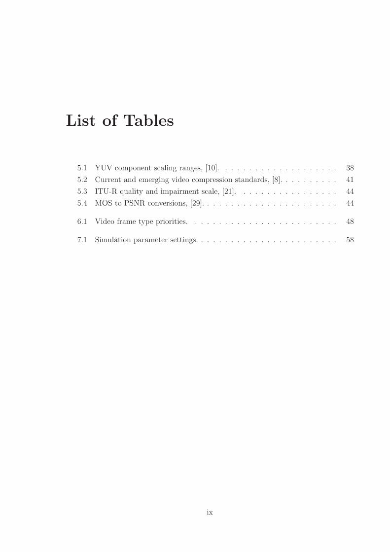
5.1 YUV component scaling ranges, [10]. . . . . . . . . . . . . . . . . . . . 38
5.2 Current and emerging video compression standards, [8]. . . . . . . . . . 41
5.3 ITU-R quality and impairment scale, [21]. . . . . . . . . . . . . . . . . 44
5.4 MOS to PSNR conversions, [29]. . . . . . . . . . . . . . . . . . . . . . . 44
6.1 Video frame type priorities. . . . . . . . . . . . . . . . . . . . . . . . . 48
7.1 Simulation parameter settings. . . . . . . . . . . . . . . . . . . . . . . . 58
ix

List of Figures
2.1 Average User Throughput of Mobile Communication Radio Access Tech-
nologies, [4]. . . . . . . . . . . . . . . . . . . . . . . . . . . . . . . . . . 8
3.1 Code division Multiplexing, [3]. . . . . . . . . . . . . . . . . . . . . . . 10
3.2 Spreading with DSSS, [3]. . . . . . . . . . . . . . . . . . . . . . . . . . 11
3.3 Near and far terminal. . . . . . . . . . . . . . . . . . . . . . . . . . . . 12
3.4 Phase Shift Keying (PSK), [3]. . . . . . . . . . . . . . . . . . . . . . . . 13
3.5 BPSK and QPSK in the phase domain, [3]. . . . . . . . . . . . . . . . . 14
4.1 High-level overview of the UMTS architecture. . . . . . . . . . . . . . . 17
4.2 UMTS architecture. . . . . . . . . . . . . . . . . . . . . . . . . . . . . . 18
4.3 UMTS packet-switched protocol architecture, [3]. . . . . . . . . . . . . 21
4.4 Radio Interface protocol architecture, [2]. . . . . . . . . . . . . . . . . . 22
4.5 MAC layer architecture, [16] . . . . . . . . . . . . . . . . . . . . . . . . 23
4.6 RLC layer architecture, [15] . . . . . . . . . . . . . . . . . . . . . . . . 24
4.7 Fundamental features to be included and excluded in HSDPA, [4]. . . . 26
4.8 General operation principle of HSDPA and associated channels, [2]. . . 27
4.9 Conceptual example of HS-DSCH code allocation with time, [5]. . . . . 27
4.10 Simplified illustration of the HSDPA architecture, [40]. . . . . . . . . . 28
4.11 MAC-hs functional entities, [20]. . . . . . . . . . . . . . . . . . . . . . . 29
5.1 Simplified illustration of a streaming server/client setup. . . . . . . . . 35
5.2 Raw video compression. . . . . . . . . . . . . . . . . . . . . . . . . . . 36
5.3 RGB colourspace, [43]. . . . . . . . . . . . . . . . . . . . . . . . . . . . 37
5.4 Example of the prediction dependencies between frames, [8]. . . . . . . 39
5.5 Playout buffer used to reduce jitter, [8]. . . . . . . . . . . . . . . . . . . 42
6.1 Data flow and SDU segmentation in the RLC layer for AM mode. . . . 47
6.2 Parameter settings for “staggered” MRED. . . . . . . . . . . . . . . . . 50
6.3 Priority drop tail overview. . . . . . . . . . . . . . . . . . . . . . . . . . 51
x

6.4 Class diagram showing existing transmission buffer constructs including
the new intermediary AQM buffers within the RLC layer. . . . . . . . . 52
6.5 Class diagram for the AQM scheme implementation. . . . . . . . . . . 53
7.1 Simulation Setup. . . . . . . . . . . . . . . . . . . . . . . . . . . . . . . 56
7.2 Comparison of frame image quality produced by each AQM scheme for
video streamed to a client at 300m using the maximum C/I scheduler. . 59
7.3 Mean PSNR when using the Round Robin Scheduler. . . . . . . . . . . 60
7.4 MOS values when using the Round Robin Scheduler. . . . . . . . . . . 60
7.5 Mean PSNR when using the Maximum C/I Scheduler. . . . . . . . . . 61
7.6 MOS values when using the Maximum C/I Scheduler. . . . . . . . . . . 61
7.7 Mean PSNR when using the Proportional Fair Scheduler. . . . . . . . . 62
7.8 MOS values when using the Proportional Fair Scheduler. . . . . . . . . 62
7.9 RLC layer packet loss when using round robin scheduler. . . . . . . . . 64
7.10 RLC layer packet loss when using maximum C/I scheduler. . . . . . . . 65
7.11 RLC layer packet loss when using proportional fair scheduler. . . . . . 65
7.12 Packet delay at 100m using round robin scheduler. . . . . . . . . . . . . 67
7.13 Packet delay at 300m using Max C/I scheduler. . . . . . . . . . . . . . 68
7.14 Packet delay at 500m using proportional fair scheduler. . . . . . . . . . 68
B.1 A Schematic of the Evalvid Framework, [21]. . . . . . . . . . . . . . . . 77
B.2 Simplified view of the NS-2 simulator, [51]. . . . . . . . . . . . . . . . . 79
xi
Chapter 1
Introduction
According to the Forbes publishing and media company [45] there were estimated
to be more than 3.5 billion cellphone subscriptions at the end of 2007. This figure is
indicative of the huge uptake by and importance of mobile communications to everyday
users worldwide. It also highlights the size of the global mobile market and the financial
gains that are possible for mobile operators today. It is no wonder, with such a large
customer base, that mobile communications companies are vying with each other for
as much of the action as they can get. The growth of the Internet has brought with
it an evolution in the way people and enterprises interact and do business with each
other. This evolution has made traditional services readily accessible to people across
towns, cities and even countries at the simple click of a button. Around the globe
mobile operators are competing with each other for mobile licences that will allow
them to setup systems and do business in as many locations as they can, especially
those with high population densities where large markets mean high returns. For mobile
operators to be successful in the future, the services that we expect from the Internet
via traditional fixed lines must also be made available via mobile technologies. With the
introduction of packet-switched services to mobile networks this is now possible. The
Internet is rapidly becoming a ubiquitous resource that is accessible to users without
the need for a fixed connection.
Today, mobile operators are providing packet-switched services based on third gen-
eration systems. When the International Telecommunication Union (ITU) started
standardising third generation systems, it intended to pave the way for a global mo-
bile system that provided a range of services including telephony, paging, messaging,
Internet and broadband data. In Europe this is being achieved through the Universal
Mobile Telecommunications System (UMTS) which is a third generation system stan-
dardised by the European Telecommunications Standards Institute (ETSI) [56]. UMTS
1
represents a natural evolution from the existing second generation GSM system, rather
than a completely new third generation system [3]. This natural evolution will prompt
mobile operators who are already using GSM to choose UMTS when upgrading their
systems rather than going for a different technology which would mean completely
changing their existing telecommunications infrastructure, thereby incurring huge ex-
pense. The UMTS system itself has been further enhanced using technologies that
provide even higher data rates than it currently supports. One of these technologies
is known as High Speed Downlink Packet Access (HSPDA), and its purpose is to im-
prove the performance for downlink packet traffic. HSDPA lies somewhere between
third and fourth generation systems and the enhancements that HSDPA offers enables
the provision of data services that require faster download rates than less demand-
ing data services. Video streaming is a multimedia service that requires higher data
rates and can be suitably handled by UMTS/HSDPA networks. Video streaming over
UMTS/HSDPA networks is the subject matter of this dissertation.
1.1 What this Dissertation is about
The objective of this dissertation is to look at the Quality of Service (QoS) of mul-
timedia traffic provided to end-users in UMTS/HSDPA networks. In particular, this
dissertation looks at video streaming and how improvements can be made by consider-
ing the operation of a specific key layer within the UMTS/HSDPA protocol architec-
ture, namely the Radio Link Controller (RLC) layer. The RLC layer can operate in
three different modes - Acknowledged mode (AM), Unacknowledged mode (UM) and
Transparent mode (TM). The 3GPP specification for the RLC layer [15], defines how
the RLC layer handles data traffic in each of these modes. It outlines how the RLC
layer stores data packets within transmission buffers. The capacity of these transmis-
sion buffers is limited by the available resources and the limits given during the radio
bearer setup. The 3GPP specification defines an SDU discard function in the RLC
layer [15]. In UM and TM, when the SDU discard function has not been configured
and the transmission buffer is full, newly arrived data packets are simply discarded.
This continues until enough room in the transmission buffer becomes available to ac-
commodate additional packets. This behaviour is similar to that of a drop-tail queue.
In AM, irrespective of whether the discard function has been configured or not, the
3GPP specification does not define the action to be taken when the transmission buffer
is full. Similar to UM and TM, in AM data packets that arrive when the buffer is full
will typically be dropped. Dropping data packets in this way may not result in the
best QoS to end-users, especially when dealing with video traffic. In this dissertation,
2

it is shown that Active Queue Management (AQM) performed at the RLC layer can
be used to improve the QoS of video traffic to end-users. Three AQM schemes are
looked at and compared. The first is a simple drop-tail scheme, which may well be
the default scheme in a real implementation. The second is a scheme based on the
well-known DiffServ architecture [25]. This scheme has already been investigated in [7]
and is included here for comparitive purposes. The third scheme is a new scheme based
on the priority treatment assigned to data packets according to their video frame type.
Simulation results are used to compare the performance of the three schemes and, in
particluar, their ability to handle video traffic and improve the QoS to end-users.
1.2 Structure of the Dissertation
This dissertation has been organized into chapters that aim to provide the necessary
background and project specific information required to understand the subject matter
of this dissertation. As such this document contains the following chapters:
Chapter 1: provides a short introduction to the subject area, describes the goal
of this dissertation and outlines the structure of this document.
Chapter 2: gives a brief account of the evolution of mobile communications.
Chapter 3: introduces the technology used in the air interface of UMTS/HSDPA
systems. Various techniques and concepts used in wireless communications and referred
to throughout this dissertation are also explained.
Chapter 4: provides a general overview of UMTS and HSDPA. Areas considered
important for the work detailed in later chapters are described here.
Chapter 5: introduces the reader to video streaming and various concepts related
to it. An overview of video compression, video standards and metrics used to analyse
video data is given. This provides the background information required to understand
the simulations performed, results obtained and analysis detailed in subsequent chap-
ters.
Chapter 6: describes Active Queue Management (AQM) in the RLC layer. The
reason for using AQM, how it can improve quality of service for video traffic, the three
schemes employed and how they have been implemented are also described.
3

Chapter 7: presents and describes the simulations performed. Results obtained
from the simulations and the evaluation and analysis of those results are also presented
in this chapter.
Chapter 8: concludes this dissertation. It summarizes the work done, draws
the main conclusions from this dissertation and outlines possible future research areas
within the domain of this dissertation.
Appendix 1: provides a list of abbreviations used throughout this dissertation.
Appendix 2: describes the tools and applications used for simulating and ana-
lyzing video traffic within UMTS/HSDPA networks. The Evalvid framework [21] that
was used to evaluate the quality of video transmitted over a simulated network is also
briefly described.
4
Chapter 2
Mobile Communications Evolution
Wireless communication systems have undergone radical technical changes over the
past forty years. Not only have drastic improvements in wireless voice communication
been made, but a whole new range of services and features can now be offered to the
user with data rates that are comparable to that of fixed line networks. These changes
and improvements have led to the creation of the UMTS/HSDPA systems that are in
use today. In order to understand how UMTS and HSDPA systems have come about, a
brief overview of the evolutionary path from first generation mobile systems up to the
present third generation ones is provided below. The chapter concludes with a preview
of up-and-coming fourth generation systems.
2.1 First Generation Systems
1G or first generation mobile phones date back to the late seventies. These signalled the
start of the mobile phone revolution. They were analog systems and used for voice com-
munication only. Several different 1G systems were launched in various places across
the globe. Of these the most important include NMT [31], AMPS [32] and CT0/1 [33].
NMT (Nordisk MobilTelefoni) was specified by the Nordic telecommunications admin-
istrations which comprised of the Scandinavian countries - Norway, Finland, Sweden
and Denmark, and later on, Iceland. AMPS (Advanced Mobile Phone System) is the
American version of the 1G analog mobile system developed by Bell Laboratories in the
United States. CT0/1 is a cordless telephone system primarily designed for domestic
use that provides a maximum range of 200m between handset and base station.
All first generation mobile systems transmitted voice signals using frequency mod-
ulation and were based on Frequency Division Multiple Access (FDMA) technology.
5

2.2 Second Generation Systems
2G or second generation mobile systems were introduced in the early nineties. In 2G
systems the former analog 1G systems were replaced by digital signal transmission
ones. SMS text messaging became possible and simple downloadable media content,
such as ringtones, were introduced. Some of the first generation systems evolved into
second generation systems, such as D-AMPS [35], GSM [34] and CT2 [36] which were
the digital 2G equivalent of the AMPS, NMT and CT0/1 1G analog systems respec-
tively. These 2G systems were based on either Frequency Division Multiple Access
(FDMA) or Time Division Multiple Access (TDMA) technology, or a combination of
both. However, cdmaOne [35] was a 2G system that had no precursor and was the
first such system to be based on Code Division Multiple Access (CDMA) technology.
A discussion on multiple access schemes is given in chapter 3.
Rather than evolving directly from second to third generation mobile systems, an
intermediary step took place that led to the creation of 2.5G systems. All previous
1G and 2G mobile systems were circuit-switched systems in which the communication
circuit (path) for the call is set up and dedicated to the participants in that call. For
the duration of the connection, all resources on that circuit are unavailable to other
users. 2.5G systems introduced packet switched networking techniques into mobile
systems. These allow the same data path to be shared by many users in the network
and potentially provides mobile users access to packet switched resources, such as the
Internet, from anywhere. Several 2.5G systems exist, the most important of which are
GPRS [37], EDGE [37] and cdma2000 [3].
2.3 Third Generation Systems
3G or third generation mobile systems came to market in early 2000. 3G systems
promised faster data rates (up to 2Mbits/s) than those provided by 2G systems and
had intended to offer high-speed Internet access, data, video and CD-quality music
services. Almost all 3G systems are based on CDMA technology of which there are
basically two variants - W-CDMA and cdma2000 [46]. W-CDMA is an extension of
the GSM system. Most GSM network providers will upgrade their systems to a W-
CDMA system known as Universal Mobile Telecommunications System (UMTS). The
reason for this is because UMTS uses much of the existing infrastructure provided by
GSM/GPRS networks and therefore a GSM/GPRS system can be easily extended to a
UMTS system. In a similar manner the 3G cdma2000 systems will be upgraded from
cdmaOne 2G systems.
6

Similarly to the intermediary step taken from 2G to 2.5G systems, 3G UMTS
systems have been enhanced, resulting in a 3.5G system. High Speed Downlink Packet
Access (HSDPA) is the UMTS enhanced 3.5G system that supports data rates of
several Mbit/s making it suitable for data applications ranging from file transfer to
multimedia streaming.
2.4 Beyond 3G - Fourth Generation Systems
The next generation of mobile systems to replace the current 3G systems have been
termed beyond 3G or simply 4G. 4G systems will improve current 3G systems in a
number of areas, including [47]:
• Support for interactive services like Video Conferencing (with more than 2 sites
simultaneously), Wireless Internet,etc.
• Much higher data transfer rates.
• Reduced data transfer costs and global mobility.
• An all digital packet network that utilizes IP in its fullest form with converged
voice and data capability.
• Improved access technologies like Orthogonal frequency-division multiplexing
(OFDM) and Multi Carrier CDMA (MC-CDMA)
• Improved security features.
4G systems are still very much in their infancy and a true description of what 4G
really means is difficult to articulate. Since the focus of this thesis is on HSDPA we will
not delve any deeper into 4G technology and the reader is referred to [38] for further
information.
2.5 Conclusion
From the first generation systems through to the current third generation the mobile
communications revolution has brought vast improvements that provide faster, more
reliable platforms of communication and access to endless amounts of information.
Since the advent of second generation mobile systems a strong focus has been on
improving data rates for packet switched services. Such services provide us with access
7

to data services such as e-newspapers, images and sound files, tele-shopping and IP-
based video telephony. With the introduction of 3G and latterly 3.5G systems new data
services that require higher data rates can now be offered, for example, video streaming
on-demand. 4G will again increase offered data rates, meaning that additional data
services will be available to consumers that could not have been offered heretofore.
Figure 2.1: Average User Throughput of Mobile Communication Radio Access Tech-nologies, [4].
In short, the mobile systems evolution has had, and continues to have, a strong
focus on increasing data rates so data services that require high data rates are pos-
sible. Figure 2.1 illustrates how average user throughput has increased for different
generations of mobile systems since packet-switched services were introduced. As mo-
bile systems continue to evolve, so data rates will continue to increase enabling the
provision of new data services and improving the Quality of Service (QoS) of existing
mobile systems.
In the following chapter various fundamentals of wireless communication are pre-
sented that are considered important for understanding later chapters. In particular
CDMA is described since it is the underlying technology used in the radio interface of
a UMTS/HSDPA system.
8

Chapter 3
Fundamentals of Wireless
Communication
This chapter introduces some fundamental principles of wireless communication. It
describes aspects of wireless communications that are referred to throughout this thesis.
Code division multiple access is described since it is the underlying technology used by
the air interface in UMTS networks. A phenomenon known as the “near/far effect” is
also explained as it relates to the fast power control technique used in UMTS networks.
Finally, phase shift keying and quadrature amplitude modulation is introduced since
it is one of the features of HSDPA explained in the following chapter.
3.1 An Overview of Medium Access Techniques
Multiplexing is the term used to describe how a communications medium is shared be-
tween different users. There are various multiplexing techniques used in communication
systems. Time division multiple access (TDMA) and frequency division multiple access
(FDMA) are two of the best known and easiest to understand techniques. TDMA is
a technique whereby time is divided into time slots and allocated to users wishing to
use the transmission medium. Within each time slot a single user uses the complete
bandwidth for the duration of the allocated time slot. When the time for the current
slot has elapsed, the next time slot is allocated to the next user and so on for each user.
To avoid interference between each consecutive user, a guard space, which is a time
gap between each users allocated time slot, is included. FDMA is a similar technique
to TDMA however rather than using time to separate the use of the communications
medium between users, frequency is used instead. All users communicate over the
medium at the same time but on different frequencies. Again guard spaces are used to
9

avoid frequency band overlapping.
TDMA and FDMA have obvious disadvantages. FDMA suffers from the fact that
the frequency spectrum is limited, thereby limiting the number of users that can gain
access to the medium. TDMA on the other hand has the disadvantage that a user who
does not use his allocated time slot wastes precious bandwidth. Additionally TDMA
also suffers when too many users are competing for time slots. When the number of
users is too great the throughput per user is reduced and thus a risk of ineffective
utilization of the medium occurs. TDMA and FDMA can be combined to increase the
overall efficacy of the medium utilization, however another technique known as code
division multiple access (CDMA) exists that provides even better utilization. This
technique is used in third generation communications systems.
3.2 Code Division Multiple Access
Code Division Multiple Access (CDMA) is a technique whereby data is transmitted
via channels that use the same bandwidth at the same time. Each channel is separated
from each other by a code, (see Figure 3.1).
Figure 3.1: Code division Multiplexing, [3].
Like TDMA and FDMA, interference between neighbouring channels is avoided by
using guard spaces, however in the case of CDMA guard spaces are used to separate
10

codes in code space. To decode the data on a specific channel, the receiver must know
the code that the transmitter used to encode it and the receiver must be precisely
synchronised with the transmitter to apply the decoding correctly. Additionally, all
signals should be received by the receiver with equal strength, otherwise some signals
could drown out the other signals. Therefore, precise power control is required.
The codes used to separate channels are called chiping sequences and their effect
is to spread the signal over the bandwidth of the transmitted signal. This technique
is known as direct sequence spread spectrum. Apart from separating channels, it also
helps to mitigate the effects of narrowband interference.
3.2.1 Direct Sequence Spread Spectrum
In order to explain direct sequence spread spectrum (DSSS) consider figure 3.2. This
diagram shows how the user data, 01, has been spread by performing an XOR with a
chipping sequence, 0110101. The result is the sequence 0110101 if the user bit equals
0, and 1001010 if the user bit equals 1.
Figure 3.2: Spreading with DSSS, [3].
The resulting sequence, 01101011001010, is what is sent over the communications
medium from the transmitter to the receiver. In order for the receiver to get the
11

original user data back, the receiver must know the original chipping sequence and
must be precisely synchronised with the transmitter. The receiver takes the received
signal and performs an XOR on it and the chipping sequence. This results in the sum
of the products equal to 0 for the first bit and to 7 for the second bit. The first sum
(0) can now map to a binary 0, and the second sum (7) can now map to a binary 1.
This makes up the original user data of 01.
Since CDMA allows multiple users to transmit messages via the same media at
the same time and across the same bandwidth, the codes used by each user must
have certain properties that allow each message to be uniquely decoded without any
distortion or overlap from other messages on the same signal. A code for a certain user
should have the properties of good autocorrelation and orthogonality. For details on
these properties see [3] and [2].
The spread spectrum technology is used in several systems, for example cdma2000
[12] and IS-95 [11]. These systems, which do not provide as high capacity as W-CDMA,
use a bandwidth of just above 1MHz compared to 5MHz for W-CDMA.
3.2.2 Near/far effect
An important phenomenon to understand when examining systems based on CDMA
is the near/far effect. It is well known that distance plays an important role in the
signal strength received by a mobile terminal. In fact the signal strength decreases
proportionally to the square of the distance between transmitter and receiver.
Figure 3.3: Near and far terminal.
Consider the situation shown in figure 3.3. Both terminals, A and C, communicate
with the base station B. As A moves further away the strength of the signal received
from it at B decreases. C may end up drowning out the signal from A and B would
12

have no chance in applying a fair scheme as it would only receive the signal from C.
The near/far effect is a severe problem for wireless networks using CDMA. All
signals arriving at the receiver must have roughly the same signal strength, otherwise
the near/far phenomenon will occur. Precise power control is required to receive all
senders with the same signal strength.
3.3 Phase Shift Keying
When transmitting digital data over a wireless medium, the binary bit stream must be
translated into an analog signal. This is the case in UMTS/HSDPA networks between
the base station and user equipment. One of the techniques employed to do this is
called phase shift keying (PSK). PSK uses shifts in the phase of the signal to
represent binary data. In figure 3.4 digital data is represented by an analog signal
where a phase shift of 180 ◦C indicates a transition from 1 to 0 and also from 0 to
1. This type of phase shifting is called binary PSK (BPSK). To receive the signal
correctly the receiver must be precisely synchronised in frequency and phase with the
transmitter.
Figure 3.4: Phase Shift Keying (PSK), [3].
As shown on the left of figure 3.5, PSK is often represented in the phase domain
which offers an alternative and typically better representation than that shown in figure
3.4. BPSK can be enhanced to provide higher bit rates by encoding two bits into each
phase shift as shown on the right of figure 3.5. This is known as quadrature PSK
(QPSK). With QPSK a phase shift of 45 ◦C represents the data 11, a phase shift of
135 ◦C represents the data 10, a phase shift of 225 ◦C represents the data 00 and a phase
shift of 315 ◦C represents the data 01. Typically the phase shifts are made relative to
a reference signal which both the transmitter and receiver must synchronize on.
13

The PSK technique can be extended to include more phase shifts at additional
angles, thereby increasing the bit rate further. Additionally, PSK can be combined
with another technique known as amplitude shift keying (ASK) where variations
in the amplitude of the analog signal represent different binary values. Combining
PSK with ASK is known as Quadrature amplitude modulation (QAM). [3] has
further details regarding PSK and QAM.
Figure 3.5: BPSK and QPSK in the phase domain, [3].
3.4 Conclusion
This chapter introduced some fundamental principles and concepts of wireless com-
munication that are especially relevant for UMTS/HSDPA networks. In the following
chapter we introduce the UMTS system that uses W-CDMA as its radio interface
and attempts to solve the near/far effect by performing power adjustments via control
channels at a rate of 1500 times a second. Enhancements to the UMTS system that
result in HSDPA are also described. One of those enhancements requires the QAM
technique described in this chapter.
14

Chapter 4
Third Generation Systems: UMTS
and HSDPA
This chapter introduces the third generation mobile telecommunications systems: Uni-
versal Mobile Telecommunications System (UMTS) and High Speed Downlink Packet
Access (HSDPA).
This chapter aims to provide an overview of the Universal Mobile Telecommunica-
tions System and describe the enhancements to it that result in High Speed Downlink
Packet Access systems. Understanding UMTS and HSDPA is a prerequisite for work
carried out as part of this thesis as described in later chapters.
4.1 Universal Mobile Telecommunications System
Universal Mobile Telecommunications System (UMTS) is a European proposal for a
third generation mobile system, which uses Wideband Code Division Multiple Access
(W-CDMA) as the air interface. UMTS extends the second generation GSM/GPRS
mobile system by reusing existing infrastructure. This is very cost effective and may
convince many operators to use UMTS if they already use GSM.
The key requirements for UMTS include:
• Minimum data rates of 144 kbits/s for rural outdoor access at a maximum speed
of 500 km/h.
• Minimum data rates of 384 kbits/s for suburban access at 120 km/h
• Up to 2 Mbit/s at 10 km/h (walking) for indoor and urban areas with relatively
short ranges.
• Provision of bearer services, real-time and non real-time services, circuit and
packet-switched transmission.
15

• Provision of many different data rates.
• Possibility of handover between UMTS cells, and between UMTS and GSM or
satellite networks.
• Compatibility between GSM, ATM, IP and ISDN-based networks.
• Provision of variable uplink and downlink data rates.
4.1.1 QoS Traffic Classes
In a UMTS network data traffic can be grouped into various classes depending on the
type and nature of the source applications and services that produce the data traffic.
Four traffic classes have been identified [2]:
• Conversational
• Streaming
• Interactive
• Background
The main distinguishing features between these classes is how delay-sensitive they
are. Conversational and streaming classes should be treated as real-time traffic and are
therefore highly delay-sensitive, with conversational traffic even more delay-sensitive
than streaming traffic. On the other hand, interactive and background traffic are
treated as non-real-time traffic and could therefore be considered within reasonable
bounds delay-insensitive, with interactive traffic less delay-insensitive than background
traffic. By considering the sensitivity levels of the individual traffic classes we can see
that each such class can be given a service priority that indicates its importance in
terms of delivery speed and delay tolerance. Listing each traffic class from the high-
est priority to lowest priority would result in the following sequence - conversational,
streaming, interactive, background - where conversational traffic has the highest prior-
ity and background the lowest priority.
4.1.2 System Architecture
A UMTS system consists of several logical network elements - the UMTS Terrestrial
Radio Access Network (UTRAN), the Core Network (CN), and the User Equipment
(UE), see figure 4.1.
Each of these elements are grouped according to the functionality they provide. The
UTRAN handles all radio-related functionality, the CN is responsible for switching and
16

Figure 4.1: High-level overview of the UMTS architecture.
routing calls and data connections to external networks, and the UE is the end-users
device that provides access to the radio interface.
UMTS provides two types of services: Circuit-switched (CS) and Packet-switched
(PS) services. CS services are services that provide access to external networks such
as ISDN or PSTN. These are typically used in traditional end-to-end telephone calls
where a dedicated connection between conversing parties is made. PS services on the
other hand are those services that provide access to external data services, such as
those accessed via the internet. Video streaming, which is the subject matter of this
dissertation, is one such example of a packet-switched service.
Figure 4.2 illustrates a simplified version of the logical elements, their sub-elements
and interfaces in the packet-switched mode of the UMTS architecture.
The UTRAN is a part of the UMTS system that has no corresponding entity in any
of the previous generation mobile communications systems. Existing elements in the
core network of the second generation GSM network have been extended to work with
UMTS. The following briefly describes the main elements of the UMTS architecture
shown in figure 4.2.
User Equipment (UE)
The UE represents the end user mobile device which contains all functions for radio
transmission as well as user interfaces. It comprises all functions needed to access
UMTS services. It performs signal quality measurements, inner loop power control,
spreading and power control modulation, and rate matching. It must also cooperate
during handover and cell selection, perform encryption and decryption and participate
in the radio resource allocation process. Additionally it performs mobility management
functions, performs bearer negotiation, or requests certain services from the network.
17
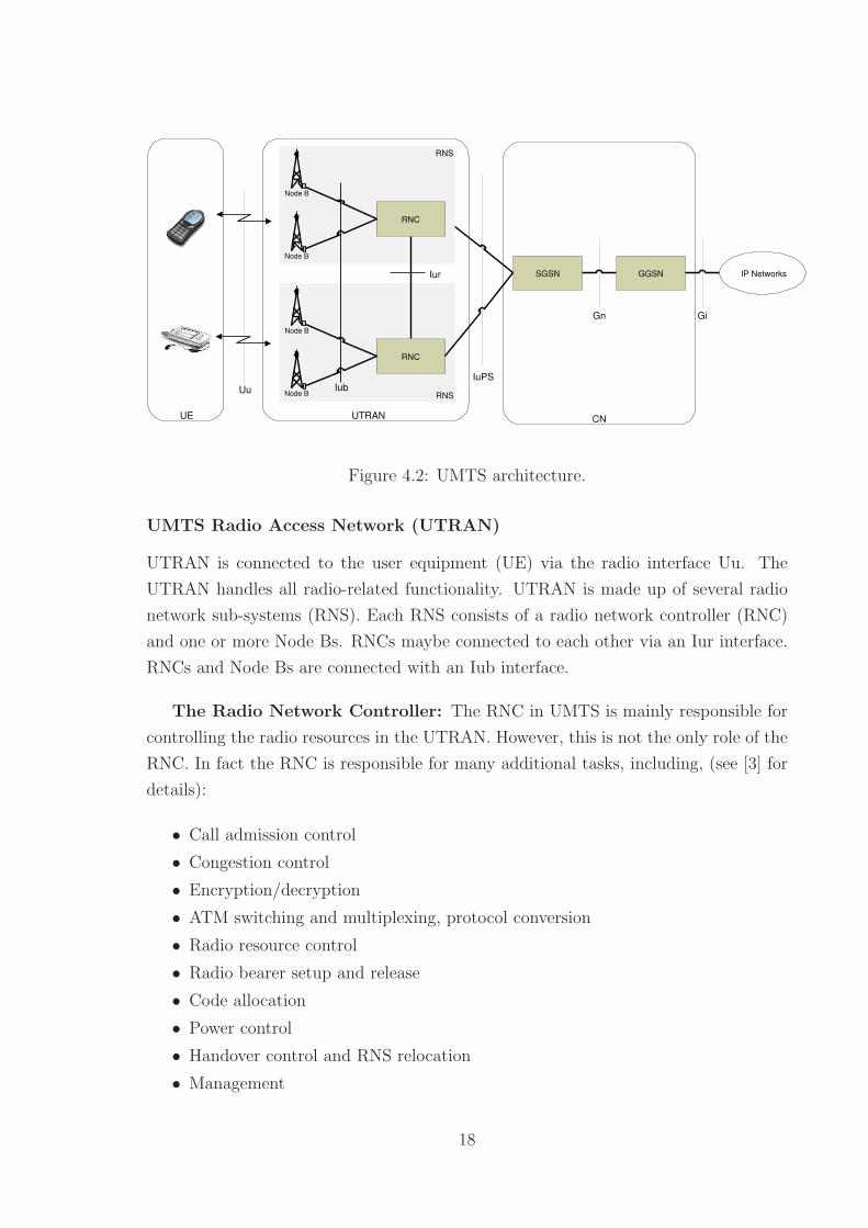
Figure 4.2: UMTS architecture.
UMTS Radio Access Network (UTRAN)
UTRAN is connected to the user equipment (UE) via the radio interface Uu. The
UTRAN handles all radio-related functionality. UTRAN is made up of several radio
network sub-systems (RNS). Each RNS consists of a radio network controller (RNC)
and one or more Node Bs. RNCs maybe connected to each other via an Iur interface.
RNCs and Node Bs are connected with an Iub interface.
The Radio Network Controller: The RNC in UMTS is mainly responsible for
controlling the radio resources in the UTRAN. However, this is not the only role of the
RNC. In fact the RNC is responsible for many additional tasks, including, (see [3] for
details):
• Call admission control
• Congestion control
• Encryption/decryption
• ATM switching and multiplexing, protocol conversion
• Radio resource control
• Radio bearer setup and release
• Code allocation
• Power control
• Handover control and RNS relocation
• Management
18

The Node B: Node B is the name given to the network component better known
in GSM terminology as the Base Station. It connects to one or more antennas creating
one or more cells. It provides the important function of inner loop power control to
minimize the effects of the near-far phenomenon. It also measures connection qualities
and signal strengths and supports soft handover between different antennas connected
to the same node B. The main function of node B is to perform the air interface
processing (channel coding and interleaving, rate adaptation and spreading, etc.) based
on W-CDMA technology.
The Iur Interface: The main functionality of the Iur interface is to allow soft han-
dover between RNCs from different manufacturers. It provides four distinct functions:
support for basic inter-RNC mobility, support for dedicated channel traffic, support
for common channel traffic, and support for global resource management. See [2] for
further details.
The Iub Interface: The Iub interface connects an RNC and a node B and defines
signalling procedures for functions such as channel handling, cell configuration and
fault configuration and management. See [2] for further details.
Core Network (CN)
The core network remains largely unchanged from that used as part of the previous
second generation GSM network with the addition of a new interface called the Iu
interface (denoted IuPS to indicate packet-switched mode). This interface is used to
connect the core network to the new UMTS radio access network (UTRAN) element.
The CN is responsible for switching and routing calls and data connections to external
networks. It contains functions for inter-system handover, gateways to other networks
and performs location management.
The SGSN (Supporting GPRS Support Node) and GGSN (Gateway Support Node)
provide functionality for packet-switched services. These two nodes existed initially as
part of the General Packet Radio Service (GPRS) extension of GSM. The GGSN is
the interworking unit between the UMTS system and the packet data networks. This
node contains routing information for mobile users, performs address conversion and
tunnels data to a user via encapsulation. The SGSN requests user addresses, keeps
track of UE locations, is responsible for collecting billing information and performing
several security functions, such as access control.
Packet data is transmitted from a packet data network via the GGSN and SGSN
directly to the RNCs. From there it is transmitted to the Node Bs and finally to the
UE.
19

The Iu Interface
This interface connects the CN to the UTRAN. As previously mentioned both packet-
switched and circuit-switched services can be provided by a UMTS system via the
CN over the Iu interface. The protocol for each type of service is different. Since we
are interested in packet-switched services figure 4.2 illustrates the Iu interface for the
packet-switched service only and as such is denoted IuPS.
The Uu Interface
The Uu interface is the W-CDMA radio interface which the UE uses to access the
fixed part of the system. It is the most important interface in the UMTS system since
it defines the protocol used for communication between the end user and the UMTS
system. The protocol stack for the Uu radio interface is further discussed in section
4.1.4.
4.1.3 Packet-Switched Protocol Architecture
The protocols over the Uu and Iu interfaces shown in figure 4.2 are divided into two
structures, [14]:
• User plane protocols: These are the protocols that implement the actual radio
bearer service that carry the user data.
• Control plane protocols: These are the protocols used for controlling the radio
access bearers and the connection between the UE and the network from differ-
ent aspects (including requesting the service, controlling different transmission
resources, handover and streamlining etc.).
The protocol structures for both planes are divided into a layered structure, similar
to the way in which the protocol stacks make up the OSI reference model. Figure 4.3
depicts the protocol architecture of the UMTS user plane providing the transmission
of user data and its associated signalling.
Basic data transport is provided by lower layers (e.g., ATM with AAL5). On top of
these layers UDP/IP is used to create a UMTS internal IP network. All packets (e.g.,
IP, PPP) destined for the UE are encapsulated using the GPRS tunnelling protocol
(GTP). The RNC performs protocol conversion from the combination GTP/UDP/IP
into the packet data convergence protocol (PDCP).
The radio layer (physical layer) can operate in two modes: frequency division duplex
(FDD) mode or time division duplex (TDD) mode. FDD mode is typically used by
20

Figure 4.3: UMTS packet-switched protocol architecture, [3].
mobile network providers, while the TDD mode is often used for local and indoor
communication. Of importance to us is the FDD mode which uses wideband CDMA
(W-CDMA) with direct sequence spreading. As implied by FDD, uplink and downlink
use different frequencies. A mobile station (otherwise known as the UE) in Europe
sends via the uplink using a carrier between 1920 and 1980 MHz, the base station uses
2110 and 2170 MHz for the downlink
The medium access control (MAC) layer coordinates medium access and multiplexes
logical channels onto transport channels. The RLC layer, among other things, performs
segmentation, reassembly and flow control. The RLC and MAC layers are further
discussed in the following sections.
4.1.4 Radio Interface Protocols
The Uu Interface briefly introduced earlier is the radio interface that allows the UE
to access the UTRAN. The protocols used across this interface are split into three
layers. Layer one is the physical layer which offers services via transport channels to
the MAC layer located in layer two. Layer two contains the MAC and RLC layers
and in the user-plane it additionally contains the Packet Data Convergence Protocol
(PDCP) and Broadcast/Multicast Control Protocol (BMC). In layer two, the MAC
layer offers services to the RLC layer via logical channels. The logical channels are
characterised by the type of data being transmitted. Layer three consists of just one
21
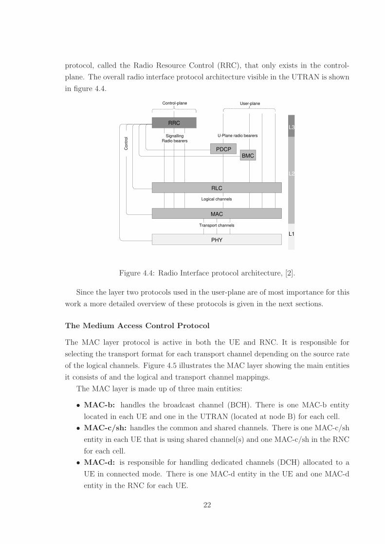
protocol, called the Radio Resource Control (RRC), that only exists in the control-
plane. The overall radio interface protocol architecture visible in the UTRAN is shown
in figure 4.4.
Figure 4.4: Radio Interface protocol architecture, [2].
Since the layer two protocols used in the user-plane are of most importance for this
work a more detailed overview of these protocols is given in the next sections.
The Medium Access Control Protocol
The MAC layer protocol is active in both the UE and RNC. It is responsible for
selecting the transport format for each transport channel depending on the source rate
of the logical channels. Figure 4.5 illustrates the MAC layer showing the main entities
it consists of and the logical and transport channel mappings.
The MAC layer is made up of three main entities:
• MAC-b: handles the broadcast channel (BCH). There is one MAC-b entity
located in each UE and one in the UTRAN (located at node B) for each cell.
• MAC-c/sh: handles the common and shared channels. There is one MAC-c/sh
entity in each UE that is using shared channel(s) and one MAC-c/sh in the RNC
for each cell.
• MAC-d: is responsible for handling dedicated channels (DCH) allocated to a
UE in connected mode. There is one MAC-d entity in the UE and one MAC-d
entity in the RNC for each UE.
22

Figure 4.5: MAC layer architecture, [16]
The functions that the MAC layer offers are described in [16]. In brief, a partial
list of MAC layer functions consists primarily of:
• Priority handling and dynamic scheduling of UEs
• Flow control between MAC layer entities
• Labelling SDUs with UE identification and various other header information
• Mapping between logical channels and transport channels
• Traffic volume monitoring
• Transport format selection for each transport channel according to the instanta-
neous source rate
The Radio Link Control Protocol
The Radio Link Control Protocol consists of RLC entities that are mainly concerned
with segmentation and retransmission services. RLC entities can be either senders or
receivers of PDUs and a sender or receiver can reside at either the UE or UTRAN.
There are three RLC entity types that are denoted by the mode they operate in:
Transparent mode (TM), unacknowledged mode (UM) and acknowledged mode (AM).
In transparent mode and unacknowledged mode a transmitting RLC entity acts as a
sender and its peer acts as a receiver. In either of these modes one transmitting and
one receiving RLC entity exists in the RLC layer. In acknowledged mode the RLC
entity is a combination of both sender and receiver.
RLC entities send and receive PDUs via lower layers along logical channels that
bind the RLC layer with the MAC layer. Higher layers are connected to the RLC layer
23
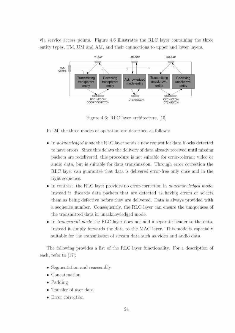
via service access points. Figure 4.6 illustrates the RLC layer containing the three
entity types, TM, UM and AM, and their connections to upper and lower layers.
Figure 4.6: RLC layer architecture, [15]
In [24] the three modes of operation are described as follows:
• In acknowledged mode the RLC layer sends a new request for data blocks detected
to have errors. Since this delays the delivery of data already received until missing
packets are redelivered, this procedure is not suitable for error-tolerant video or
audio data, but is suitable for data transmission. Through error correction the
RLC layer can guarantee that data is delivered error-free only once and in the
right sequence.
• In contrast, the RLC layer provides no error-correction in unacknowledged mode.
Instead it discards data packets that are detected as having errors or selects
them as being defective before they are delivered. Data is always provided with
a sequence number. Consequently, the RLC layer can ensure the uniqueness of
the transmitted data in unacknowledged mode.
• In transparent mode the RLC layer does not add a separate header to the data.
Instead it simply forwards the data to the MAC layer. This mode is especially
suitable for the transmission of stream data such as video and audio data.
The following provides a list of the RLC layer functionality. For a description of
each, refer to [17]:
• Segmentation and reassembly
• Concatenation
• Padding
• Transfer of user data
• Error correction
24

• In-sequence delivery of upper layer PDUs
• Duplicate detection
• Flow control
• Sequence number check
• Protocol error detection and recovery
• Ciphering
• SDU discard
• Out of sequence SDU delivery
• Duplicate avoidance and reordering
The Packet Data Convergence Protocol
The Packet Data Convergence Protocol (PDCP) is only used in the user plane in
the packet-switched domain. Its main function is to provide header compression of
redundant control information at the transmitting entity and decompression at the
receiving entity. The reason why this is done becomes more apparent when the size of
a typical RTP/UDP/IP header is considered. For IPv4 the combined header size is at
least 40 bytes. For IPv6 it is at least 60 bytes. The payload for IP voice can be 20
bytes or less. By providing header compression a significant reduction in the overall
data packet size can be achieved. [18] provides details about the PDCP protocol.
The Broadcast/Multicast Control Protocol
Within the UTRAN there is only one Broadcast/Multicast Control (BMC) protocol
entity per cell. The BMC Protocol exists only in the user plane and is designed to adapt
broadcast and multicast services originating on the radio interface to a geographical
area mapped into cells. It is responsible for storing, scheduling, transmission and
delivery of broadcast messages and traffic volume monitoring. [19] provides details
about the BMC protocol.
4.2 High Speed Downlink Packet Access
Higher data rates and larger system capacity is required to supply the growing demand
of evolving mobile communications markets. To meet these demands one of the tech-
nologies that has been been standardized in the 3GPP release 5 standard, [13], is a new
technology denominated High Speed Downlink Packet Access (HSDPA). High-Speed
Downlink Packet Access is a mobile telephone protocol in the High-Speed Packet Ac-
cess (HSPA) family of third generation technologies designed to increase data transfer
25
rates “with methods already known from Global System for Mobile Communications
(GSM)/Enhanced data rates for global evolution (EDGE) standards, including link
adaptation and fast physical layer retransmission combining” [2].
HSDPA falls into the category of 3.5G technologies since it is an enhancement to
the current UMTS 3G system. Theoretical peak download speeds of up to 14.4Mbits/s
have been specified, making it ideal for multimedia streaming and video and data
downloads.
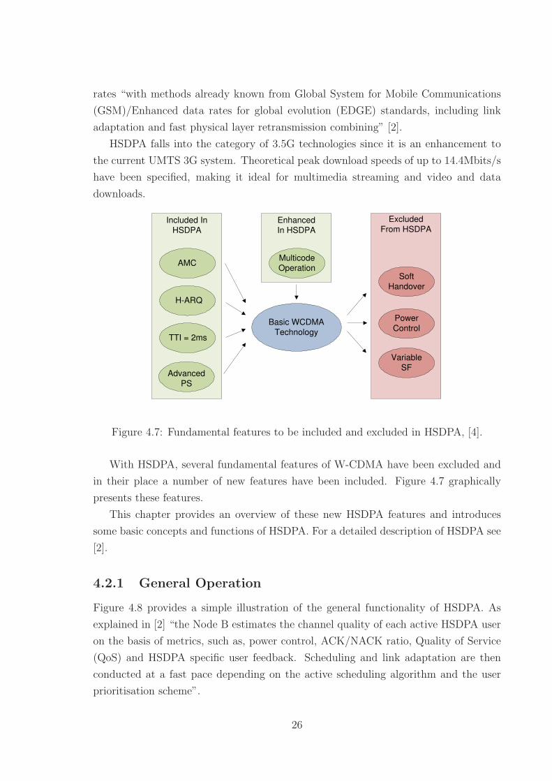
Figure 4.7: Fundamental features to be included and excluded in HSDPA, [4].
With HSDPA, several fundamental features of W-CDMA have been excluded and
in their place a number of new features have been included. Figure 4.7 graphically
presents these features.
This chapter provides an overview of these new HSDPA features and introduces
some basic concepts and functions of HSDPA. For a detailed description of HSDPA see
[2].
4.2.1 General Operation
Figure 4.8 provides a simple illustration of the general functionality of HSDPA. As
explained in [2] “the Node B estimates the channel quality of each active HSDPA user
on the basis of metrics, such as, power control, ACK/NACK ratio, Quality of Service
(QoS) and HSDPA specific user feedback. Scheduling and link adaptation are then
conducted at a fast pace depending on the active scheduling algorithm and the user
prioritisation scheme”.
26

Figure 4.8: General operation principle of HSDPA and associated channels, [2].
In HSDPA user data is carried on the downlink to UEs via a new transport channel
called the High-speed Downlink Shared Channel (HS-DSCH). The HS-DSCH works in
conjunction with the high-speed shared control channel (HS-SCCH) which is responsi-
ble for carrying key information for HS-DSCH demodulation.
The High Speed Dedicated Physical Control Channel (HS-DPCCH) is a new HS-
DPA uplink channel and is described in [44] as a channel created to carry both
ACK/NACK information for the physical layer retransmissions as well as the downlink
channel quality indicator (CQI) which provides feedback information used by the Node
B scheduler for determining the terminal to transmit to and the data rate used.
Figure 4.9: Conceptual example of HS-DSCH code allocation with time, [5].
27
All HSDPA devices within a cell share the the HS-DSCH resource on a time and
code multiplexed basis. [5] explains that 15 available unique codes can be “re-used
in each 2ms transmission time interval (TTI). For each TTI, the base station fast
scheduling algorithm allocates 0-15 codes to each user device currently awaiting data
in the cell”. This concept is illustrated in Figure 4.9. [5] goes on to explain that
“in theory each code can be used to deliver data with an effective rate of 960Kbps
(960Kbps/code x 15codes = 14.4Mbps). However, in practice, the base station will
have to select a lower effective data rate”.
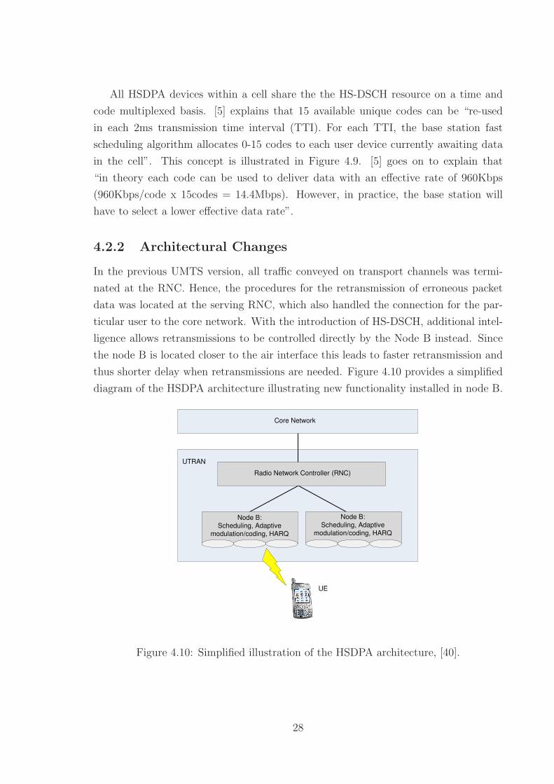
4.2.2 Architectural Changes
In the previous UMTS version, all traffic conveyed on transport channels was termi-
nated at the RNC. Hence, the procedures for the retransmission of erroneous packet
data was located at the serving RNC, which also handled the connection for the par-
ticular user to the core network. With the introduction of HS-DSCH, additional intel-
ligence allows retransmissions to be controlled directly by the Node B instead. Since
the node B is located closer to the air interface this leads to faster retransmission and
thus shorter delay when retransmissions are needed. Figure 4.10 provides a simplified
diagram of the HSDPA architecture illustrating new functionality installed in node B.
Figure 4.10: Simplified illustration of the HSDPA architecture, [40].
28
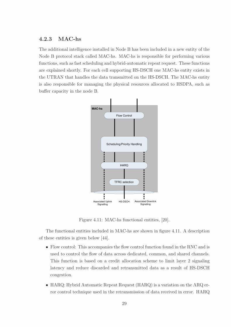
4.2.3 MAC-hs
The additional intelligence installed in Node B has been included in a new entity of the
Node B protocol stack called MAC-hs. MAC-hs is responsible for performing various
functions, such as fast scheduling and hybrid-automatic repeat request. These functions
are explained shortly. For each cell supporting HS-DSCH one MAC-hs entity exists in
the UTRAN that handles the data transmitted on the HS-DSCH. The MAC-hs entity
is also responsible for managing the physical resources allocated to HSDPA, such as
buffer capacity in the node B.
Figure 4.11: MAC-hs functional entities, [20].
The functional entities included in MAC-hs are shown in figure 4.11. A description
of these entities is given below [44].
• Flow control: This accompanies the flow control function found in the RNC and is
used to control the flow of data across dedicated, common, and shared channels.
This function is based on a credit allocation scheme to limit layer 2 signaling
latency and reduce discarded and retransmitted data as a result of HS-DSCH
congestion.
• HARQ: Hybrid Automatic Repeat Request (HARQ) is a variation on the ARQ er-
ror control technique used in the retransmission of data received in error. HARQ
29

allows data blocks received in error to be combined with retransmitted data
blocks, thereby increasing the likelihood of successfully decoding the transport
block. HARQ is further explained in the next section.
• Scheduling/Priority handling: This entity manages HS-DSCH resources that are
allocated to users based on their priority. A further description of the scheduling
function is given in the following sections.
• TFRC selection: This entity is used to select an appropriate transport format
and resource combination (TFRC) for the data to be transmitted on HS-DSCH.
In the following section the main HSDPA features are described including the two
major functional entities in MAC-hs, the scheduler and the HARQ unit.
4.2.4 Features
Shorter TTI
In order to provide fast scheduling and improved modulation and coding rates HSDPA
Channel quality information is obtained every 2ms. As explained in [5] “the 2ms TTI
used in HSDPA is considerably shorter than the typical 10 to 40ms range used in earlier
UMTS releases. Because various transmission parameters can be modified within each
TTI, a shorter TTI allows the system to adapt itself more quickly to changing radio
conditions”.
Higher Order Modulation
In chapter 3 phase shift keying (PSK) and quadrature amplitude modulation, (QAM)
were introduced. During early feasibility studies 8 PSK and 64 QAM were considered,
but eventually these schemes were discarded for performance and complexity reasons.
In their place, HSDPA uses 16 QAM radio modulation which can double the rate of
traditional UMTS QPSK modulation for those users who receive high signal strength
relative to the level of inter-cell interference.
Fast Packet Scheduling and Adaptive Modulation and Coding
Resource management is performed by a packet scheduler that may decide to serve a
particular user based on any one of a number of characteristics. One of these charac-
teristics may be the channel quality information. By scheduling users only when their
channel conditions are good enough the scheduler reduces the likelihood of transmis-
sion errors and therefore improves cell throughput. However, the packet scheduler may
30

also decide to schedule users based on fairness rather than throughput. This could
be achieved by scheduling users in a round robin fashion, irrespective of their channel
quality information. Various scheduling algorithms are available that alter the way in
which the scheduler operates but basically each scheduler aims to dynamically allocate
a variable proportion of the shared HS-DSCH resource, (i.e. a number of codes, from
0-15). Various schedulers are described in section 4.2.5.
As well as being used to contribute to the scheduling decision, [5] explains that
the channel quality indicator (CQI) information “is used to determine the adaptive
modulation and coding (AMC) parameters that will reliably deliver the highest data
rate to that device (the calculation is actually based on a 10% expected error rate to
ensure that the system always runs close to the limit). AMC determines the modula-
tion scheme (16QAM or QPSK), and the amount of error protection overhead to be
used. Data to be sent by HSDPA is Turbo encoded to provide a high level of error pro-
tection - effectively tripling the amount of data that would have to be sent. The AMC
process determines how much error protection overhead can be removed according to
the reported CQI.
Thus the useful data rate (after decoding) that is transmitted to each device is
determined by the number of allocated codes, the type of modulation and the amount
of error protection. In this way, fast scheduling and AMC attempt to optimise HSDPA
transmission to increase the likelihood of successful reception by devices whilst ensuring
the highest possible data rates.
This useful transmitted data rate is therefore directly related to the CQI reported by
the device and can typically vary between 69Kbps/code and 717Kbps/code, compared
to the theoretical maximum of 960Kbps/code.
After completing fast scheduling, the base station signals to the selected device that
they will receive data in the next TTI and informs them of the corresponding AMC
parameters”.
HARQ
HSDPA has improved the way in which erroneous data was previously treated by
rapidly retransmitting missing transport blocks through the use of the fast Hybrid
ARQ (HARQ) technique.
As [5] again explains: “HSDPA employs a stop and wait hybrid automatic repeat
request (SAW HARQ) retransmission protocol between the base station and the user
device. With HARQ, each device checks the integrity of its received data in each rele-
vant HS-DSCH TTI. If the data is correct, the device returns an ACK (acknowledging
31
the receipt of correct data) signal, in which case the base station can move to transmit
the next set of data.
If the data is not successfully received, the device transmits an NACK (negative
acknowledgement) and the base station retransmits the corresponding data”. With
soft-combining, UEs do not discard the erroneous frames, but combine them with the
successive retransmitted frames using schemes like Chase Combining and Incremental
Redundancy.
4.2.5 More about Scheduling
As explained in section 4.2.1, data is carried to HSDPA users via the channel denoted
HS-DSCH. Data destined for different users can be simultaneously carried on this chan-
nel on a time and code multiplexed basis. Every transmission time interval (i.e. 2ms)
a new set of users, the previous users or a mixture of both new and existing users may
expect data on the HS-DSCH resource. In order to share the HS-DSCH resource be-
tween users a fast packet scheduler is employed. Its fundamental task is to schedule the
transmission of data to users. The data to be transmitted to users is placed in different
queues in a buffer located at node B and the scheduler determines the sequential order
in which the data streams are sent. Previously, in the release ’99 UTRAN architecture
scheduling was performed at the RNC, [14]. For HSDPA, scheduling has been moved
to the new MAC-hs entity in the the protocol stack of node B. Scheduling has also been
moved to the node B in order to take advantage of the improved efficiency that can be
gained from being as close to the air interface as possible. By placing the scheduler at
node B transmission delays, that may otherwise occur, are reduced. Moreover it allows
quick access to the diverse and varying channel characteristics used to make scheduling
decisions.
The HSDPA scheduler is the key to resource management on the downlink channel
because it decides which user, or set of users, is to be scheduled in each transmission
time interval. The scheduler aims to improve system throughput while maintaining
satisfactory QoS for users by taking a number of factors into consideration. These
factors include the channel quality, terminal capability, fairness between users, cell
throughput, QoS class and power/code availability. The type of scheduler used may
involve a trade-off between these factors. Numerous schedulers have been proposed and
studied in the literature. According to [6] the three most commonly used scheduling
algorithms are:
• Round-Robin (RR)
32

• Maximum Carrier to Interference ratio (Max C/I)
• Proportional Fair (PF)
These are briefly described in the next sections.
Round-Robin (RR) Scheduling
This algorithm selects users in a round robin fashion. As [1] explains: “In this method,
the number of time slots allocated to each user can be chosen to be inversely propor-
tional to the user’s data rates, so the same number of bits is transmitted for every
user in a cycle. Obviously, this method is the “fairest” in the sense that the average
delay and throughput are the same for all users. However, there are two disadvantages
associated with the round-robin method. The first is that it disregards the conditions
of the radio channel for each user, so users in poor radio conditions may experience
low data rates, whereas users experiencing good channel conditions may not receive
any data until the channel conditions become poor again. This is obviously against
the spirit of HSDPA and would lead to the lowest system throughput. The second dis-
advantage of the round-robin scheduler is that there is no differentiation in the quality
of service provided to different classes of users”.
Maximum Carrier to Interference ratio (Max C/I) Scheduling
As [1] again explains: “In this method, the scheduler attempts to take advantage of
the variations in the radio channel conditions for different users, and always chooses to
serve the user experiencing the best channel conditions, that is, the one with maximum
carrier-to-interference ratio”. This can be explained as follows [7]: “If Ri(t) is the
instantaneous data rate experienced by user i at time t, then the CI scheduler assigns
the slot at time t to the user j having the maximum value of the index:
pj = Rj(t) (4.1)
i.e. it gives the channel to the user able to achieve the highest instantaneous data
rate.” The maximum C/I scheduler leads to the maximum system throughput but is
the most unfair, as users in poor radio conditions may never get served or suffer from
unacceptable delays.
Proportional Fair (PF) Scheduling
This method takes into account both the short-term variation of the radio channel
conditions and the long-term throughput of each user. In this method [1]: “the user
33
that is served first is the one that maximises the following:
pi = Ri(t)/li(t) (4.2)
where Ri(t) is the instantaneous data rate experienced by user i and li(t) is the
average data rate for the user in the past average window. The size of the average
window determines the maximum duration that a user can be starved of data, and,
as such, it reflects the compromise between the maximum tolerable delay and the
cell throughput. According to this scheme, if a user is enjoying a very high average
throughput, its Ri(t)/li(t) will probably not be the highest. It may then give way to
other users with poor average throughput and therefore high Ri(t)/li(t) in the next
time slot, so the average throughput of the latter can be improved. On the other hand,
if the average throughput of a user is low, the Ri(t)/li(t) could be high and it might
be granted the right of transmission even if its current channel conditions are not the
best”.
4.3 Conclusion
This chapter has introduced UMTS and outlined the HSDPA enhancements that enable
higher data rates than was previously possible. An overview of the UMTS protocol
architecture and radio interface protocols was provided. Among the layers that make
up the radio interface protocols attention was paid to the RLC layer. Additionally,
HSDPA has been explained in broad terms and with emphasis on fast scheduling.
A good understanding of the RLC layer and scheduling algorithms described in
this chapter is necessary for understanding the work performed and described in later
chapters of this thesis.
34

Chapter 5
Video Streaming: Concepts and
Measurement Metrics
5.1 Introduction
According to [41]: “Streaming is a technical re-ordering of data that makes it possible
for a user to view and interact with media information without having to wait for it
to download entirely to his or her computer. Instead of waiting for a 5 (or 10 or 50)
megabyte file to be transferred over the internet, a process which could take hours,
a user is able to begin viewing the material while later portions of the presentation
continue to download in the background, ready to be shown when they are needed,
which is called buffering.”
Figure 5.1: Simplified illustration of a streaming server/client setup.
A user can view a streamed video file on a client machine by accessing a streaming
server located at a specific address. (See figure 5.1). The streaming server may be
located on the same network as the client, or even at a remote location somewhere on
the internet. Normally the streaming server is paired with a web server. It is general
practice to have the streaming server running on a different machine to the web server
35
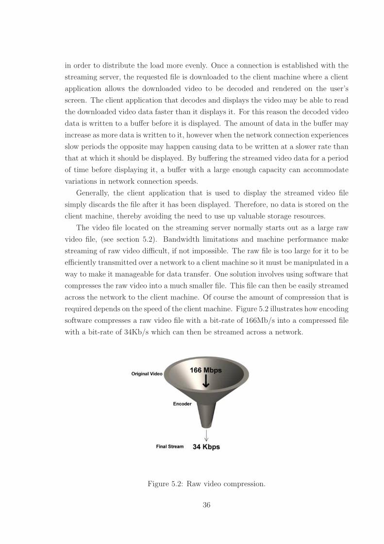
in order to distribute the load more evenly. Once a connection is established with the
streaming server, the requested file is downloaded to the client machine where a client
application allows the downloaded video to be decoded and rendered on the user’s
screen. The client application that decodes and displays the video may be able to read
the downloaded video data faster than it displays it. For this reason the decoded video
data is written to a buffer before it is displayed. The amount of data in the buffer may
increase as more data is written to it, however when the network connection experiences
slow periods the opposite may happen causing data to be written at a slower rate than
that at which it should be displayed. By buffering the streamed video data for a period
of time before displaying it, a buffer with a large enough capacity can accommodate
variations in network connection speeds.
Generally, the client application that is used to display the streamed video file
simply discards the file after it has been displayed. Therefore, no data is stored on the
client machine, thereby avoiding the need to use up valuable storage resources.
The video file located on the streaming server normally starts out as a large raw
video file, (see section 5.2). Bandwidth limitations and machine performance make
streaming of raw video difficult, if not impossible. The raw file is too large for it to be
efficiently transmitted over a network to a client machine so it must be manipulated in a
way to make it manageable for data transfer. One solution involves using software that
compresses the raw video into a much smaller file. This file can then be easily streamed
across the network to the client machine. Of course the amount of compression that is
required depends on the speed of the client machine. Figure 5.2 illustrates how encoding
software compresses a raw video file with a bit-rate of 166Mb/s into a compressed file
with a bit-rate of 34Kb/s which can then be streamed across a network.
Figure 5.2: Raw video compression.
36
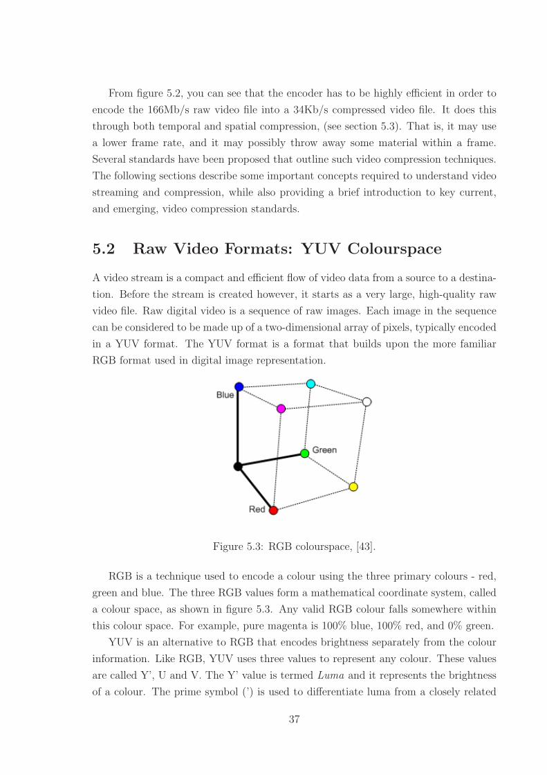
From figure 5.2, you can see that the encoder has to be highly efficient in order to
encode the 166Mb/s raw video file into a 34Kb/s compressed video file. It does this
through both temporal and spatial compression, (see section 5.3). That is, it may use
a lower frame rate, and it may possibly throw away some material within a frame.
Several standards have been proposed that outline such video compression techniques.
The following sections describe some important concepts required to understand video
streaming and compression, while also providing a brief introduction to key current,
and emerging, video compression standards.
5.2 Raw Video Formats: YUV Colourspace
A video stream is a compact and efficient flow of video data from a source to a destina-
tion. Before the stream is created however, it starts as a very large, high-quality raw
video file. Raw digital video is a sequence of raw images. Each image in the sequence
can be considered to be made up of a two-dimensional array of pixels, typically encoded
in a YUV format. The YUV format is a format that builds upon the more familiar
RGB format used in digital image representation.
Figure 5.3: RGB colourspace, [43].
RGB is a technique used to encode a colour using the three primary colours - red,
green and blue. The three RGB values form a mathematical coordinate system, called
a colour space, as shown in figure 5.3. Any valid RGB colour falls somewhere within
this colour space. For example, pure magenta is 100% blue, 100% red, and 0% green.
YUV is an alternative to RGB that encodes brightness separately from the colour
information. Like RGB, YUV uses three values to represent any colour. These values
are called Y’, U and V. The Y’ value is termed Luma and it represents the brightness
of a colour. The prime symbol (’) is used to differentiate luma from a closely related
37

value, luminance, which is designated Y. Luminance is derived from linear RGB values,
whereas luma is derived from non-linear (gamma-corrected) RGB values. The prime
symbol is frequently omitted, but YUV colour spaces always use luma, not luminance.
Luma is derived from an RGB colour by taking a weighted average of the red, green,
and blue components. For standard-definition television, the following formula, taken
from specification ITU-R BT.601 [10], is used:
Y ′ = 0.299R + 0.587G + 0.114B (5.1)
This formula reflects the fact that the human eye is more sensitive to certain wave-
lengths of light than others, which affects the perceived brightness of a color. Blue
light appears dimmest, green appears brightest, and red is somewhere in between.
The U and V components, also called chroma values or color difference values, are
derived by subtracting the Y value from the red and green components of the original
RGB color as follows:
U = B − Y ′ (5.2)
V = R − Y ′ (5.3)
Together, these values contain enough information to recover the original RGB
value.
One of the big advantages of using the YUV format over the RGB format is to
do with the fact that the human eye is more sensitive to changes in brightness than
it is to changes in hue. This means that an image can have less chroma information
(U and V) than luma information (Y’) without sacrificing the perceived quality of the
image. For example, it is common to sample the chroma values at half the horizontal
resolution of the luma samples. In other words, for every two luma samples in a row
of pixels, there is one U sample and one V sample.
The formulas previously given for YUV are not the exact conversions used in digital
video. Digital video generally uses a form of YUV called Y’CbCr. Essentially, Y’CbCr
works by scaling the YUV components to the ranges shown in table 5.1. For further
details see the ITU-T BT.601 recommendation [10].
Component Range
Y’ 16-235
Cb/Cr 16240, with 128 representing zero
Table 5.1: YUV component scaling ranges, [10].
38

5.3 Video Compression: Frame Types
Raw video files are made up of a sequence of uncompressed still images where each
image is a frame in the video sequence. Compression of a raw video file can be thought
of as a two-step process. Firstly, each still image contained in a frame in the video
sequence is encoded using an image compression technique, such as JPEG, TIFF, GIF,
etc. Secondly, similarities between image frames in the video sequence are exploited to
compress the video file even further.
A better understanding of the two step video compression process is as follows: For
the first step, consider image compression, such as that defined by the JPEG standard.
The JPEG standard encodes raw, still images resulting in a much smaller version of
the original. Compression techniques are used that exploit the high similarities found
between neighbouring pixels within the image. In fact, generally small 8×8 pixel blocks
are taken and compared with neighbouring blocks of the same size. The motivation
for using small block sizes is that the pixels within a small block are more likely to
be similar than those within larger blocks. For each 8 × 8 block the JPEG standard
computes the 2-D Discrete Cosine Transform (DCT) for each block. Each 8×8 block of
DCT coefficients is then quantized and processed using a number of techniques known
as zigzag scanning, run-length coding, and Huffman coding to produce a compressed
bitstream [9].
Figure 5.4: Example of the prediction dependencies between frames, [8].
In the second step of the video compression process, consider each still image con-
tained in a frame in the video sequence. Sequential frames will be highly similar and
therefore the similarities between these frames can be exploited. This allows a further
level of compression at the frame level in addition to the JPEG-like compression at the
image level previously explained. As described in [8], frame level compression is most
effectively achieved by (1) predicting successive frames based on preceding frames, and
39

then (2) by coding the error in this prediction. Consecutive video frames typically
contain the same imagery, however possibly at different spatial locations because of
motion. Therefore, to improve the predictability it is important to estimate the mo-
tion between the frames and then to form an appropriate prediction that compensates
for the motion. The process of predicting motion between frames is known as motion
estimation (ME). When a frame is to be coded it is split into 16× 16 pixel blocks and
for each block a prediction is found by finding the best-matching block in a previously
coded-frame.
The MPEG standard defines three types of coded frames, namely I, P and B frames.
The following briefly explains them:
• I-Frame: This is the intra-frame and it is coded independently of all other frames.
It acts as an anchor point upon which other frame types are dependant. If an
I-frame becomes lost successive dependant P and B frames cannot be decoded.
• P-Frame: This is the predicted-frame. It depends on the previous I or P-frame
which may or may not be the frame directly preceding it.
• B-Frame: This is the bidirectional predicted-frame. It depends on surrounding I
and P-frames.
Figure 5.4 illustrates the different type of coded frames and the dependencies be-
tween them for a sample MPEG Group of Pictures.
5.4 Video Compression Standards
Many standards for video compression exist. In general, each standard has been cre-
ated to specify the bit stream syntax, that represents the compressed data format, and
the decoding process, that is the set of rules for interpreting the bit-stream. Specific
implementations have not been standardized in order to give designers and manufac-
turers greater creative freedom and to avoid limitations that would exist if a restrictive
and prescriptive standard for all parts in a compression process were enforced.
Two families of video compression standards currently exist. These are the outcome
of the activity of video experts of the ITU-T and ISO. Table 5.2 summarizes the main
standards defined by the ITU-T and ISO and shows their designed operational bit
rates. For details about these standards see [48] and [49].
1p = 1,2,...30 multiples of the baseline ISDN data rate.
40

Video CodingStandard
Primary Intended Applications Bit Rate
H.261 Video telephony and teleconferenc-ing over ISDN
p1x 64 kb/s
MPEG-1 Video on digital storage media (CD-ROM)
1.5 Mb/s
MPEG-2 Digital Television 2-20 Mb/s
H.263 Video telephony over PSTN 33.6 kb/s and up
MPEG-4 Object-based coding, synthetic con-tent, interactivity, video streaming
Variable
H.264/MPEG-4 Part10 (AVC)
Improved video compression 10s to 100s ofkb/s
Table 5.2: Current and emerging video compression standards, [8].
H.264, also known as MPEG-4 Part 10, is one of the standards jointly created
by the ITU-T and ISO. It is the most recent video compression standard created by
both bodies and is likely to dominate applications like IPTV and digital video broad-
cast. As stated in [42], the H.264 standard was developed in response to the growing
need for higher compression of moving pictures for various applications such as video-
conferencing, digital storage media, television broadcasting, Internet streaming, and
communication. It is also designed to enable the use of the coded video representa-
tion in a flexible manner for a wide variety of network environments. The Standard
allows motion video to be manipulated as a form of computer data and to be stored
on various storage media, transmitted and received over existing and future networks
and distributed on existing and future broadcasting channels.
5.5 Metrics
When studying video data and video streaming, it is important to realize what proper-
ties are important and how they effect the quality of the video as seen by an end-user.
Knowing and understanding the various metrics that can be measured is a require-
ment in any experimental undertaking. The following sections provide an introduction
to the most common metrics available for comparing and analysing streamed video
data. These metrics will be used to analyze and evaluate results obtained from the
simulations performed during the course of this work.
41

5.5.1 Delay Jitter
There are a number of factors that affect the quality of video received by an end-user.
One of these factors is called delay jitter. This is a phenomenon that results when
data packets are received at different rates. The different rates arise due to variations
in end-to-end delay caused by, for example, queuing delays, traffic congestion in the
network, packet loss resulting in retransmission of packets, or any other number of
factors.
One key effect of delay jitter is that a jerky video sequence is seen by the end-user.
A video sequence consists of a number of frames that must be sequentially viewed at a
constant rate and in the proper order to view the video as intended. Variations in end-
to-end delay may cause variations in the frame rate resulting in a jerky video sequence.
To get around this problem a technique known as buffering is used. Buffering can reduce
delay jitter by making use of a playout buffer whose task is to buffer incoming frame
data before displaying it to the user. Ultimately, the video application waits an amount
of time until enough frames have been buffered before playing back the streamed video
sequence. This effectively extends the display deadline of frames within the video
sequence and in most cases will remove delay jitter entirely. Figure 5.5 illustrates
the advantages of buffering where playback is delayed until enough packets have been
buffered to compensate for any further delays that may occur in the network.
Of course, the amount of buffering is dependant on the application area, and in some
cases minimal or no buffering is permissible. This is typical of real-time applications
where delays are not tolerated. An example of this would be video conferencing where
the video at the receiving end must be simultaneous with zero delay.
Figure 5.5: Playout buffer used to reduce jitter, [8].
42

5.5.2 Packet loss
Packet loss is a phenomenon whereby packets of data are lost during transmission and
never arrive at their final destination. There may be a number of reasons for packet
loss in a network and the type of network involved may give rise to different types
of losses. For example, in a fixed network packet loss may result in complete packets
being erased. Whereas wireless networks are typically afflicted by bit errors and burst
errors.
With respect to video streaming, packet loss is an important factor that can have a
large effect on video quality. Since video frames are generally bigger than the maximum
transfer unit (MTU) of the network they are normally segmented into many smaller
packets that are each the size of one MTU or smaller. These packets are streamed
across the network and then concatenated at the receiving end, recreating the original
frames which can then be decoded and viewed. Packet loss during transmission across
the network can have a detrimental effect on video quality since the decoder may not
be able to decode the frame if it has not been able to reconstruct the frame properly
given that some data is missing.
There are techniques that can be used to combat packet loss. These techniques
fall roughly into four classes of error control: forward error correction, retransmissions,
error concealment, and error-resilient video coding. An overview of these four classes
of error control can be found in [8].
Analyzing packet loss is a valuable metric for determining video quality and it is
used during the evaluation of the work described herein.
5.5.3 PSNR/MOS
According to [29], “video quality measurements must be based on the perceived quality
of the actual video being received by the users of the digital video system. Such a
perception-based evaluation is appropriate as the subjective impression of the user is
what only counts ultimately”. In other words, a real test of video quality can only be
performed when a person looks at the video and provides a rating based on his/her
subjective opinion. A metric that users can use to rate the quality of the actual video
has been proposed by the ITU and is known as the Mean Opinion Score or MOS. The
MOS is a scale that allows users to rate video on a scale from 1 to 5 as shown in Table
5.3.
Unfortunately using subjective approaches for measuring video quality is extremely
expensive in terms of time, resources and financial cost. As such, alternative methods
for measuring video quality have been investigated and one of the most common of
43

Scale Quality Impairment
5 Excellent Imperceptible
4 Good Perceptible, not annoying
3 Fair Slightly annoying
2 Poor Annoying
1 Bad Very annoying
Table 5.3: ITU-R quality and impairment scale, [21].
these is an objective approach based on the calculation of peak-signal-to-noise ratio
(PSNR). PSNR compares the peak signal energy to noise energy of video components
on a frame by frame basis. Due to the greater effect that the Y component has on a
video image (see section 5.2), PSNR is often based only on the luminance component
of the video. Equation (5.4) illustrates how the source and destination luminance
components are used to define the PSNR between the source image S and destination
image D, [21].
PSNR(n)dB = 20 log10
Vpeak√
1(NcolNrow)
∑Ncol
i=0
∑Nrow
j=0 [YS(n, i, j) − YD(n, i, j)]2(5.4)
Vpeak = 2k− 1
k = number of bits per pixel (luminance component)
As explained in [29], a mapping exists between PSNR and MOS values as shown
in table 5.4. This is useful in order to present a more user-friendly view of the video
quality, and indirectly provides subjective analysis of video quality using an objective
approach.
PSNR [dB] MOS
> 37 5 (Excellent)
31 -37 4 (Good)
25 - 31 3 (Fair)
20 - 25 2 (Poor)
< 20 1 (Bad)
Table 5.4: MOS to PSNR conversions, [29].
44

Both PSNR and MOS values are used as evaluation metrics on simulations per-
formed and described in chapter 7.
5.6 Conclusion
This chapter has introduced some important video streaming concepts. Most impor-
tantly, video encoding and the frame types that are created as a result of video encoding
have been explained and the metrics used to analyze and evaluate video quality have
been introduced. An understanding of these areas is required in order to further un-
derstand the work carried out as part of this thesis.
45

Chapter 6
Active Queue Management in the
RLC Layer
This chapter introduces the idea of using active queue management in the RLC layer
of the RNC to improve the QoS of video traffic in a UMTS/HSDPA network. The
reason for using active queue management in the RLC layer is due to random packet
dropping under overloaded conditions resulting in poor video quality at the receiver.
This problem is described in the first section of this chapter. The next section contains
a description of how the video frame type can be used by active queue management
schemes to improve the video quality. Various active queue management schemes are
then introduced. This lays the foundation for the simulations described in chapter 7.
Finally, the last section explains how the AQM schemes previously described have been
implemented in NS2.
6.1 Data Flow and Packet Drops in the RLC Layer
Figure 6.1 illustrates a simplified overview of the data flow in the RLC layer when
transmitting data to a recipient. It shows how the RLC layer receives data traffic from
the upper PDCP layer in the form of an RLC Service Data Unit (SDU). A segmen-
tation function is responsible for taking the newly arrived RLC SDUs and segmenting
them into payload units (PU) of a predefined size. The PU size is defined during the
radio bearer setup phase and can only be changed through the radio bearer reconfigu-
ration procedure. After segmentation and buffering the RLC layer performs RLC PDU
construction and ciphering tasks. Finally the RLC PDU is then passed to the MAC
layer ready for transmission.
46

Figure 6.1: Data flow and SDU segmentation in the RLC layer for AM mode.
An important point to note is that the transmission buffer has a finite capacity
and there may be a time when it is too full to accommodate any further segmented
RLC SDUs. In [15], the RLC specification describes an RLC SDU discard function
that, under certain conditions when the transmission buffer is too full, causes a newly
arrived RLC SDU to be discarded instead of segmented and queued as previously
described. With respect to video traffic this can have wide-ranging implications on
the QoS delivered to the end user. For instance, it is more than likely due to packet
fragmentation within the network that an individual RLC SDU arriving at the RLC
layer represents only a portion of a complete video frame. If an RLC SDU that is part
of a video frame is discarded, the video decoder will find it challenging when it tries to
decode a frame if not all the RLC SDUs that make up that frame are available. The
more RLC SDUs that are missing, the more difficult it will be for the video decoder to
decode the frame. Obviously efforts should be made to avoid this situation. Of course
due to resource limitations there may not be enough buffer space to accommodate
all traffic. However, discarding some RLC SDUs while allowing the remainder to be
transmitted may be a waste of bandwidth if the video decoder at the receiving side
cannot decode the frame to acceptable levels given the subset of RLC SDUs that it
receives. Active queue management can be used to address all of these problems.
47
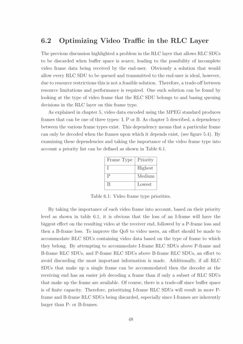
6.2 Optimizing Video Traffic in the RLC Layer
The previous discussion highlighted a problem in the RLC layer that allows RLC SDUs
to be discarded when buffer space is scarce, leading to the possibility of incomplete
video frame data being received by the end-user. Obviously a solution that would
allow every RLC SDU to be queued and transmitted to the end-user is ideal, however,
due to resource restrictions this is not a feasible solution. Therefore, a trade-off between
resource limitations and performance is required. One such solution can be found by
looking at the type of video frame that the RLC SDU belongs to and basing queuing
decisions in the RLC layer on this frame type.
As explained in chapter 5, video data encoded using the MPEG standard produces
frames that can be one of three types: I, P or B. As chapter 5 described, a dependency
between the various frame types exist. This dependency means that a particular frame
can only be decoded when the frames upon which it depends exist, (see figure 5.4). By
examining these dependencies and taking the importance of the video frame type into
account a priority list can be defined as shown in Table 6.1.
Frame Type Priority
I Highest
P Medium
B Lowest
Table 6.1: Video frame type priorities.
By taking the importance of each video frame into account, based on their priority
level as shown in table 6.1, it is obvious that the loss of an I-frame will have the
biggest effect on the resulting video at the receiver end, followed by a P-frame loss and
then a B-frame loss. To improve the QoS to video users, an effort should be made to
accommodate RLC SDUs containing video data based on the type of frame to which
they belong. By attempting to accommodate I-frame RLC SDUs above P-frame and
B-frame RLC SDUs, and P-frame RLC SDUs above B-frame RLC SDUs, an effort to
avoid discarding the most important information is made. Additionally, if all RLC
SDUs that make up a single frame can be accommodated then the decoder at the
receiving end has an easier job decoding a frame than if only a subset of RLC SDUs
that make up the frame are available. Of course, there is a trade-off since buffer space
is of finite capacity. Therefore, prioritizing I-frame RLC SDUs will result in more P-
frame and B-frame RLC SDUs being discarded, especially since I-frames are inherently
larger than P- or B-frames.
48

6.3 Video Traffic Management Schemes
In the following, three queuing schemes are introduced that propose various ways of
dealing with the RLC SDU discard problem for video traffic. The first is a simple drop
tail scheme. The second is a scheme based on the Differentiated Services Architecture
[25]. The third is a new priority drop tail scheme. Both the Differentiated Services and
the priority drop tail schemes make use of the idea of prioritizing frames as suggested in
the previous section. [7] also describes the use of the differentiated services scheme as a
means to improve the QoS for video traffic in UMTS/HSDPA networks, however, a new
scheduler is incorporated into the tests performed. This makes it difficult to realize how
much of an improvement in QoS can be attributed solely to the differentiated services
scheme implemented. In the tests performed and described in this thesis a comparison
between each AQM scheme provides a means of evaluating the effect on QoS of video
traffic for a particular scheme precisely.
6.3.1 Drop Tail Scheme
The drop tail scheme is the simplest of the queuing schemes looked at and may well
be the default scheme in many RLC layer implementations. Drop tail schemes treat
all incoming RLC SDUs indifferently and can fully utilize the transmission buffer’s
complete capacity. This may be appropriate for data packets that are considered
equally important, but for data such as video traffic a drop tail scheme may drop
packets that are of greater importance than those that have been queued. For example,
if a P-frame RLC SDU takes up the remaining space in the transmission buffer, the
following I-frame RLC SDU will be discarded if the buffer is still full on the I-frame’s
arrival. The drop tail scheme drops all RLC SDUs with a probability of 1 when the
buffer is full, irrespective of the data being carried by the RLC SDU.
6.3.2 DiffServ Scheme
The DiffServ scheme is based on the differentiated services architecture defined in [25].
The differentiated services architecture is an IP based QoS architecture that divides
user traffic into different classes based on user requirements. Data traffic belonging
to a class is marked with a code point that indicates how it should be treated by the
network. In addition to traffic classification, each traffic class can be given different
dropping precedences. The dropping precedences allow differential treatment of traffic
within a single class. DiffServ implements a mechanism known as Assured Forwarding
Per Hop Behaviour, (AF PHB), [28] which has been standardized by the IETF and
49

specifies four classes with three levels of drop precedence. The AF PHB mechanism
implemented by DiffServ makes use of the Multi-Level RED (MRED) active queue
management technique described in [27]. MRED is based on the well known Random
Early Detection (RED) algorithm, [26], and can be considered to act like a set of RED
queues running in parallel, where each RED queue is associated with a given drop
precedence. The dropping probability of packets associated with a specific drop prece-
dence is based on the average queue size and a minimum and maximum threshold.
The average queue can be calculated using a number of different schemes. The scheme
used in the simulations shown in chapter 7 is the RIO-C variant [27].
Figure 6.2: Parameter settings for “staggered” MRED.
For video traffic each data packet is marked with the frame type. Each frame
type represents a drop precedence that has the priority shown in table 6.1. The RED
parameters for each type are staggered as figure 6.2 illustrates. This shows that B-
frames will be dropped earlier and with a higher probability than P- or I-frames.
P-frames will be dropped next with a higher probability than I-frames. And I-frames
will be dropped last with a lower probability than P- and B-frames.
6.3.3 Priority Drop Tail Scheme
The priority drop tail scheme is a mixture of both the simple drop tail and DiffServ
schemes previously described. The priority drop tail scheme maintains three buffers,
one for each of the video frame types - I, P and B - as figure 6.3 shows.
Similar to DiffServ, a marking strategy allows data packets to be marked at source
with the type of video frame they are part of - I, P or B. On arrival at the RLC layer this
information can be used to decide to which buffer the newly arrived RLC SDU should
50

Figure 6.3: Priority drop tail overview.
be added. The aggregate size of the buffers should not exceed the maximum buffer
size defined during the radio bearer setup. A pointer keeps track of the RLC SDUs so
that when dequeuing the RLC SDUs from each of the buffers they are dequeued in the
order they were added. When the total size of all the buffers exceeds the maximum
allowed buffer size a priority algorithm is initiated. This algorithm is responsible for
discarding lower priority RLC SDUs from its buffer in order to make room for higher
priority RLC SDUs in its buffer. This is done in a hierarchical manner where space
is made for higher priority RLC SDUs by dropping RLC SDUs from lower priority
buffers, starting at the lowest priority buffer. If all RLC SDUs have been dropped
from the lowest priority buffer and the aggregate size of all the buffers plus the size of
the incoming higher priority RLC SDU is greater than the overall allowed maximum
buffer size, RLC SDUs will be dropped from the next highest priority buffer. This
continues until enough room is available to accommodate the incoming higher priority
RLC SDU. Like the drop tail scheme, the priority drop tail scheme makes use of the
transmission buffers full capacity by dropping RLC SDUs only when it has to. It also
makes sure that the low priority RLC SDUs are dropped only when need be, and high
priority RLC SDUs are always queued as long as the maximum buffer size permits it.
In fact, as long as the transmission buffer size is big enough, RLC SDUs belonging to
the highest priority frame types should never be dropped. This scheme is simple yet
effective as the results in chapter 7 illustrate.
6.4 Implementing Active Queue Management in NS2
NS2 [51] is a network simulation tool used to simulate various network scenarios. Eu-
rane [50] is an extension to NS2 that can be used to model UMTS and HSDPA networks.
An overview of NS2 and Eurane is given in Appendix B. In NS2 the UTRAN is simu-
lated by the EURANE plug-in. The RLC layer is implemented in detail and provides
51

per-user queues and a credit-based algorithm used by the RLC layer to calculate the
number of RLC PDUs to be passed to the MAC layer at each TTI. The transmission
buffers in the RLC layer in NS2 are implemented using a Vector construct and there
is one transmission buffer for each flow created in the TCL script. In addition, each
transmission buffer contains as many priority queues as there are priority types. The
number of priority types is defined by the traffic types defined in the TCL script. Gen-
erally there are no more than 4 types, one for each of the standard UMTS traffic types
described in chapter 4. The priority queues are implemented using the umtsQueue
class type. Due to complexities within the EURANE code, rather than perform active
queue management directly on the transmission buffers’ associated priority queues,
RLC SDUs are fed into an intermediary buffer where active queue management is per-
formed. These intermediary buffers are implemented using the AQM class type. From
the intermediary buffers, the RLC SDUs are passed to the transmission buffers. This
leaves the existing code intact and extracts out the new code without affecting the
original process flow in the existing code. In figure 6.4 a partial class diagram of the
RLC layer is shown. This illustrates the structure of the transmission buffers in NS2
and also the addition of the new intermediary buffers for active queue management.
Figure 6.4: Class diagram showing existing transmission buffer constructs includingthe new intermediary AQM buffers within the RLC layer.
The intermediary buffers can be managed using any of the three active queue man-
52

agement schemes previously described - drop tail, DiffServ or Priority drop tail. These
have been implemented using the strategy pattern so that any of the schemes can be
easily selected at runtime by setting a parameter in the TCL script using tcl binding.
Each scheme is implemented in a class that extends the AqmBase class. The Aqm-
Base class is an abstract class that defines all the default functions that any base class
should implement. Adding a new AQM scheme simply requires that the new scheme
be implemented in a class that extends AqmBase and that the AQM context class is
configured with the new class. A class diagram illustrating the three AQM schemes,
the base class, context class and their relationships are shown in Figure 6.5.
Figure 6.5: Class diagram for the AQM scheme implementation.
6.5 Conclusion
This chapter has provided an overview of the packet dropping problem at the RLC
layer. The priority level of the video frame type has been introduced as a solution to
the packet dropping problem. Two AQM schemes based on the priority level of the
video frame type have been discussed along with a drop-tail scheme that may be the
default implementation in the RLC layer of a typical system. Integrating the AQM
schemes into NS2 has also been explained. The following chapter employs these AQM
53

schemes and performs simulations which yield results that can be used to compare and
demonstrate the effectiveness of each of the schemes described here.
54
Chapter 7
Video Streaming: Network
Simulation, Evaluation And
Analysis
This chapter describes simulations performed, and results obtained, using a combina-
tion of the NS2 simulator [51], Eurane plugin [50], and Evalvid framework [21]. The
objective is to compare how effective the different RLC layer AQM algorithms de-
scribed in chapter 6 prove to be for video traffic when used alongside various HSDPA
schedulers for changing BS to UE distances. Performance and effectiveness are mea-
sured in terms of end-to-end delay, packet loss and PSNR values. For evaluating video
quality an additional metric based on the PSNR values is also used, called the mean
opinion score (MOS).
7.1 Simulation Description
Figure 7.1 shows the network topology used to simulate and evaluate video traffic in a
UMTS/HSDPA network. Modelling the UMTS/HSDPA network was provided by the
Eurane extension to NS2, [50]. In addition to the source node that represents a video
server for streaming video traffic to an end-user, a number of extra source nodes repre-
senting the four UMTS traffic classes described in chapter 4 are included to provide a
mix of different traffic within the simulated network. In total 9 mobile users are down-
loading data from 9 source nodes via Node-B using TCP and UDP connections. Within
the simulation there are 4 TCP and 5 UDP connections. The 4 TCP connections are
made up of 2 connections running FTP and 2 connections running Pareto (ON/OFF)
distributed traffic. The 5 UDP connections are made up of 2 exponential (ON/OFF)
55

connections representing conversational traffic and 3 connections representing video
traffic.
The end users (UEs) are configured to act as pedestrians, each moving with a speed
of 3km/hour at average distances of between 100 and 500 metres from the base station.
Since packet loss is a critical factor that affects the perceived video quality at the
receiver, the intermediary nodes located before the RNC have been configured so that
no packet loss or congestion occurs before the RNC. In addition, the RLC layer is
configured to operate in acknowledgement mode so that once RLC SDUs are placed
in the transmission buffer they are guaranteed to be delivered. In other words, the
only place where packets can be dropped is when an attempt to add RLC SDUs to the
transmission buffer in the RLC layer of the RNC occurs. This means that the quality
of the received video can be solely attributed to packet loss in the RLC layer.
Figure 7.1: Simulation Setup.
For video traffic, tasks such as packetization, packet sequence numbering and in-
order delivery are normally provided by higher-layer protocols such as the Real-Time
Protocol (RTP). In the simulations here this protocol is not modeled, however, the
tasks that this protocol provides are supported by a number of tools that come as part
of the Evalvid framework [21]. Within Evalvid a raw YUV sequence is encoded into
MPEG4 format using a compatible encoder. The MPEG4 video used in the simulations
56

consists of 300 frames running at a rate of 30 frames/second over a 10 second duration.
No B-type frames were produced by the encoder. The MPEG4 stream is fed into a
trace file generator that parses and packetizes the MPEG4 file into a format that can
then be used as an input traffic generator to the simulation. The format of the input
is a file containing the packet sequence number, packet size and frame type of every
packet in the video sequence. After running the simulation, the result is an output
trace file that contains delay data, packet sequence number, packet size and frame
type of every packet received. Finally, Evalvid provides a number of tools that use the
trace and video files to reconstruct the video as would be seen by the user. It also
allows the calculation and extraction of PSNR, delay and various other metrics that
can be used in the evaluation of video quality. Appendix B has more details about
the Evalvid framework and the toolset it provides for video simulation, analysis and
evaluation.
Table 7.1 provides a summary of the parameters and their input values used in the
simulations. The results of the simulations are given in the following sections.
7.2 Results
The following describes results gathered and compiled when streaming video traffic over
the UMTS/HSDPA simulated network shown in figure 7.1. These results are used to
compare the performance and effectiveness of the different RLC layer AQM algorithms
described in chapter 6 when handling video traffic. Metrics, such as end-to-end delay,
packet loss and PSNR values, are used to evaluate the different AQM algorithms. For
evaluating video quality an additional metric based on the PSNR values is also used,
called the mean opinion score (MOS). Using subjective metrics is too complex and
expensive to make them feasible, so an automated approach that emulates the quality
impression of the human visual system is employed by means of the MOS metric [21].
The MOS metric was previously described in subsection 5.5.3.
Figure 7.2 shows an example frame taken from the video sequence received by a
user after a network simulation has been performed. Each image in figure 7.2 provides
a shot of the same frame when different AQM algorithms are used in the RLC layer. It
is obvious to see that a subjective test would point at the default Drop Tail algorithm
as producing the lowest quality of all three algorithms. When examining the DiffServ
and Priority Drop Tail algorithms the difference at first may not appear to be quite so
great. However, on closer examination the microphone and shirt of the news reader in
the image produced by the DiffServ algorithm can be seen to be less sharp than that
of the Priority Drop Tail algorithm. Using the example shown in figure 7.2 is a good,
57

Parameter Name Input Values
Video parametersVideo format CIF (352x288)Frame rate 30 frames/secondNumber of frames 300Video encoding MPEG4
TTI 2 msHARQ cycle period 6CQI Delay in TTI 3Multipath fading environment Pedestrian AUser Speed 3.0 km/hUser Distance to Base Station 100 m to 500 mLinit, Distance loss at 1 km 137.4PTx, BS Transmission power 38 dBmGT, BS antenna gain 17 dBiPath loss exponent 3.52Iintra, intra-cell interference 30 dBmIinter, inter-cell interference -70 dBmShadowing parameters
Standard deviation 8 dBCorrelationdistance 40 m
Number of streaming (video) users 3Number of background (FTP) users 2Number of interactive (web) users 2
Traffic model Pareto-distributedPareto shape parameter 1.1Pareto packet size parameter 240Pareto burst time parameter 1.60 sPareto idle time parameter 5 sPareto rate parameter 60 kbps
Number of conversation (VOIP) users 2Traffic model Exponential-distributedExponential packet size parameter 240Exponential burst time parameter 1.60 sExponential idle time parameter 5 sExponential rate parameter 60 kbps
RLC mode AMPDU Size 40 bytesMax MAC-hs buffer size 500 PDUsMax RLC Transmission buffer size Q 1000 PDUsDiffServ parameters
minThB , maxThB 0.5Q, 0.7QminThP , maxThP 0.7Q, 0.8QminThI , maxThI 0.8Q, 1.0QmaxPB 0.6maxPP 0.5maxPI 0.01Average weight wq 0.9
Simulated time 20 seconds
Table 7.1: Simulation parameter settings.
58

Figure 7.2: Comparison of frame image quality produced by each AQM scheme forvideo streamed to a client at 300m using the maximum C/I scheduler.
once-off, demonstration of the improvements that the different algorithms can make.
However, doing this on a frame by frame basis would be far to costly in terms of time
and effort so we turn instead to alternative means of comparison.
In figures 7.3, 7.4, 7.5, 7.6, 7.7 and 7.8 graphs illustrating the mean PSNR and
MOS values for each of the different AQM algorithms at varying distances from the
Base station are shown. Each set of graphs illustrates the results when a different
HSDPA scheduler has been selected in the MAC-hs layer of the Base station. As can
be seen, the Priority Drop Tail algorithm maintains higher average PSNR values than
the other two AQM algorithms across the range of distances from 100 metres to 500
metres from the base station, no matter what MAC-hs scheduler is chosen. The best
average PSNR values for the Priority Drop Tail algorithm itself are achieved when
used in combination with the round-robin scheduler. The average PSNR values for
the Priority Drop Tail algorithm, when used in combination with the proportional-fair
algorithm, closely match the performance achieved when the round-robin scheduler is
used. The Priority Drop Tail algorithm used with the Maximum C/I scheduler returns
slightly worse results as the video user moves further away from the base station.
Since Maximum C/I bases its scheduling decisions on channel conditions, which are
ultimately affected by distance to base station, the slightly degraded outcome when
using the Maximum C/I scheduler is expected.
59
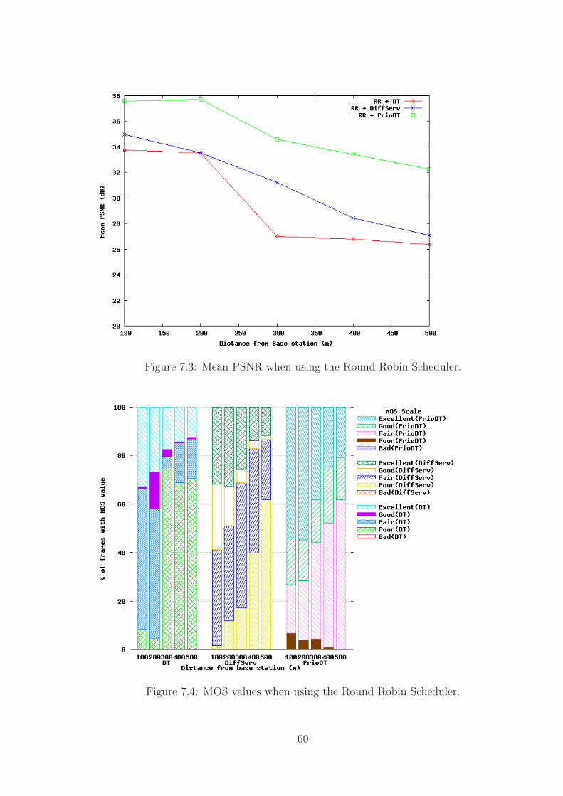
Figure 7.3: Mean PSNR when using the Round Robin Scheduler.
Figure 7.4: MOS values when using the Round Robin Scheduler.
60

Figure 7.5: Mean PSNR when using the Maximum C/I Scheduler.
Figure 7.6: MOS values when using the Maximum C/I Scheduler.
61

Figure 7.7: Mean PSNR when using the Proportional Fair Scheduler.
Figure 7.8: MOS values when using the Proportional Fair Scheduler.
62

In addition to the average PSNR values, graphs showing the MOS score are given,
providing an alternative approach to assessing the video quality. Taking the MOS val-
ues obtained when using the round-robin scheduler as an example, it can be clearly seen
that again the Priority Drop Tail algorithm delivers the best results. Analyzing the
graph for each of the AQM algorithms shows that the combined percentage of excellent
and good frames is highest for the Priority Drop Tail algorithm, far outweighing those
of the other two AQM algorithms.
Looking at the graphs in figures 7.3 to 7.8, it can be seen that the Priority Drop
Tail algorithm delivers the best results in terms of PSNR and MOS values for all BS
to UE distances and for all schedulers. One reason for this is that the Priority Drop
Tail algorithm does not discard any RLC SDUs that make up I-frames so long as it
can accommodate them. This results in delivery of all RLC SDUs needed to make up
complete I-frames at the receiver. Since I-frames are much larger than P- or B-frames
they will have a greater effect on PSNR values (and hence MOS values). The DiffServ
algorithm tries to achieve the same objectives, however, since it does not use the full
buffer capacity the higher values achieved by the Priority Drop Tail algorithm are not
possible. On the other hand, the Drop Tail algorithm drops RLC SDUs indifferently
and so incomplete frames are received by the end-user resulting in lower values.
Of course there is a trade-off when prioritizing data packets based on their frame
type. Figures 7.9, 7.10 and 7.11 illustrate this. These figures show the number of RLC
SDU packets carrying I- and P-frame type data received by the end-user. Missing
packets are determined to have been discarded by the RLC layer. Due to the maxi-
mum packet size imposed by the network, the 300-frame video sequence used in the
simulations has been fragmented into 979 packets of which 160 are I-frame type packets
and 819 are P-frame type packets. By looking at the graphs it is clear to see that for
the Priority Drop Tail algorithm a trade-off exists that results in high I-frame type
packet throughput at the expense of higher P-frame type packet drops. In fact, the
Priority Drop Tail algorithm maintains the complete 160 I-frame type packets with a
lower P-frame type packet throughput across all distances for all schedulers, except at
large distances from the base station when using the Maximum C/I scheduler. Since
the transmission buffers have limited capacity and the Maximum C/I scheduler gives
preference to UEs with higher CQI values, it is inevitable that at some point I-frame
type packets will be lost as the receiving UE moves further away from the base sta-
tion and the transmission buffer reaches its maximum limit. The DiffServ algorithm
follows the Priority Drop Tail algorithm closely but does not manage to maintain the
same high levels of I-frame type packet throughput. However, it does achieve higher
levels of P-frame type packet throughput at greater BS to UE distances. This is due
63

to the fact that the Priority Drop Tail algorithm dequeues P-frame type packets to
make room for I-frame type packets, whereas the DiffServ algorithm keeps P-frame
type packets once they have been queued, even if it means that the next incoming I-
frame type packet must be dropped due to lack of space. The Drop Tail algorithm may
appear to achieve higher total packet throughput because it always maintains higher
levels of P-frame type packets than the other AQM algorithms. However, firstly the
Drop Tail algorithm drops more I-packets than either of the other AQM algorithms
and secondly I-frame type packets are, on average, bigger in size than P-frame type
packets. Therefore, looking at throughput based on packet size instead of number of
packets, the Priority Drop Tail algorithm outperforms the other two AQM algorithms.
Figure 7.9: RLC layer packet loss when using round robin scheduler.
64

Figure 7.10: RLC layer packet loss when using maximum C/I scheduler.
Figure 7.11: RLC layer packet loss when using proportional fair scheduler.
65

A question that may be raised over the Diffserv and Priority Drop Tail AQM
algorithms is how much extra overhead do they introduce into the RNC and hence,
how effective are these algorithms when compared to the default implementation. The
extra processing required to read the frame type and process the packet according to
the AQM algorithm is indeed an important factor that is worth some investigation. The
effect that these algorithms have on the performance of the network can be measured by
comparing the end-to-end packet delay of each and also comparing the results against
the default Drop Tail algorithm. Figures 7.12, 7.13 and 7.14 provide graphs that
illustrate the end-to-end packet delay for each AQM algorithm for a randomly selected
sample of UE to BS distances and MAC-hs schedulers. RLC SDU Packets that have
zero delay are packets that have been discarded by the RLC layer according to the
AQM algorithm implemented. Since the delay between each node in the simulated
network has been fixed, and delay within nodes outside the UTRAN is negligible,
processing within the RLC and MAC-hs layers accounts for any additional delay. In
fact, the peaks in figures 7.13 and 7.14 can be directly attributed to the scheduler in
the MAC-hs layer of the BS. In both cases the transmission buffer fills quickly with
RLC SDUs. However, the transmission buffer will not be emptied until it is scheduled
to do so. Figure 7.13 illustrates the end-to-end delay of video data streamed to a UE
located 300 metres away from the base station. The Maximum C/I scheduler serves all
other UEs with a better CQI value before the UE streaming the video data is served,
resulting in several delay peaks. The initial peak is larger than any of the other peaks.
This can be attributed to the fact that a sudden large burst of data arrives at the
RNC from various sources at the same time. Since web and VOIP traffic are bursty
in nature this is a common phenomenon found in any network. If UEs receiving this
bursty traffic have better CQI values than that of the UE streaming the video data,
then the video data remains in the transmission buffer until the scheduler has serviced
all others with higher CQI values. This explains the first large peak in figure 7.13.
Thereafter, a number of smaller bursts of traffic occur resulting in less spectacular
peaks. A similar explanation can be used for figure 7.14.
It can be seen from these graphs that, despite the extra processing required by
the Diffserv and Priority Drop Tail AQM algorithms, they still roughly follow the
same general shape of the default Drop Tail AQM algorithm. In fact the average end-
to-end delay is less for the Diffserv and Priority Drop Tail AQM algorithms than it
is for the Drop Tail AQM algorithm. Since the delay throughout the network out-
side the UTRAN is fixed and the delay due to the MAC-hs scheduler should be the
same for all cases, the difference in delay can be directly attributed to variations in
processing at the RLC layer. Since I-frame type packets are on average larger than
66

P-frame type packets, it takes less I-frame type packets to fill the transmission buffer.
This means that less processing is needed to fill the transmission buffer with I-frame
type packets. Since both the Diffserv and Priority Drop Tail AQM algorithms aim
to preferentially buffer all I-frame type packets over P-frame type packets the differ-
ence in delay must be caused by the effect of the additional processing of the larger
number of P-frame type packets processed by the default Drop Tail AQM algorithm.
Figure 7.12: Packet delay at 100m using round robin scheduler.
67

Figure 7.13: Packet delay at 300m using Max C/I scheduler.
Figure 7.14: Packet delay at 500m using proportional fair scheduler.
68
7.3 Conclusion
In this chapter simulations using NS2 and the Eurane extension that provide a means
of analysing and evaluating the different AQM schemes outlined in the previous chapter
have been described. The use of the Evalvid framework to encode a raw YUV video
sequence into MPEG4 format, generate input and output trace files and analyse the
resultant video through the use of several metrics have been explained. The results
have shown better PSNR and MOS values and average end-to-end delay for the Priority
Drop Tail scheme when compared to the DiffServ and Drop Tail schemes.
The following chapter concludes this dissertation by summarizing the work un-
dertaken and outlining possible future avenues of research that build upon the work
undertaken as part of this dissertation.
69
Chapter 8
Conclusions and Future Work
Mobile telecommunications covers a huge subject area and becoming familiar with it
without any prior knowledge, even in a general sense, takes a big effort. During the
course of this dissertation I have endeavoured to become familiar with mobile telecom-
munications, focus on some key areas and gain exposure to technologies which were
unknown to me before. I have had the fortune of researching some very interest-
ing and important areas of mobile telecommunications and through this research I
have gained knowledge in some of the latest technologies, including UMTS/HSDPA,
WCDMA, Video Streaming and Active Queue Management. In addition to this I have
also had a chance to work with various simulation tools, mainly NS2, and associated
software applications and this has led to some good hands-on experience of C++. From
the knowledge I have gained during the research period I have been able to examine
UMTS/HSDPA networks, analyze the protocol architecture of these networks and fo-
cus on a specific layer of that architecture, namely the RLC layer. This work has
exposed the problem of random packet dropping from transmission buffers in the RLC
layer. Active Queue Management has been suggested as a means to alleviate the ran-
dom packet dropping problem found. Various AQM schemes have been proposed and
analysed and a new Priority Drop-Tail scheme has been shown to improve the QoS of
video traffic to end-users when compared to the default Drop-tail scheme and an AQM
scheme based on the well known Differentiated Services architecture, [25]. The com-
parisons made between the different AQM schemes show QoS improvements for video
traffic based on end-to-end delay, packet loss in terms of frame type, Peak-signal-to-
noise ratio and Mean Opinion Score. A well-defined framework for video evaluation
was used for this purpose, [21].
70

8.1 Future Work
Although Active Queue Management at the RLC layer has been shown to improve
the video quality received by the end-user, further ways of improving the QoS of
video traffic to end-users are required. Additional problems or areas of improve-
ment have been identified that may further affect video quality and provide scope
for further investigation and exploration into the area of video streaming improve-
ments over UMTS/HSDPA networks. The following highlights some of these areas.
Active Queue Management based on Data Packet sets: The Differentiated
Services and Priority Drop-Tail AQM schemes presented in chapter 6 use the video
frame type as a marking mechanism to prioritize data packets in the RLC layer. Al-
though these schemes make a best effort to hold on to data packets for high priority
frames, data packets for lower priority frames maybe dropped. This may lead to a
problem at the receiving end where data packets are concatenated to recreate video
frames. Each data packet contains partial information for a complete video frame. If
data packets for lower priority frames are dropped only part of the full set of packets
needed to make up a complete video frame maybe received making it more difficult for
the decoder to decode the partially received frame. Most video decoders have in-built
algorithms that are capable of dealing with this type of situation to a certain extent,
however, as more and more data packets become lost the decoder will find it increas-
ingly difficult to decode the frame given the partial data set it receives. When too many
data packets are missing, the decoder will not be able to produce a video frame of high
enough quality to render it acceptable to a viewer. Passing a subset of data packets to
the receiver that render bad quality images could be considered a waste of bandwidth
and system resources. This highlights an area of investigation that could be examined
for potential improvements to video quality where an AQM scheme could be devel-
oped that controls the flow of data packets based on the frame to which they belong!
HSDPA Scheduling based on Traffic Type: During the course of this disserta-
tion, many HSDPA schedulers were studied. Of all the HSDPA scheduling algorithms
looked at none were found to use the UMTS traffic classes as a basis for scheduling.
Chapter 4 introduced the four UMTS traffic classes and explained that each class can
be categorized according to how delay-sensitive it is. Delay sensitivity can be used as a
means of prioritizing each traffic class, where highly delay sensitive traffic is considered
high priority and traffic that is less delay sensitive is considered low priority. Since video
streaming belongs to a traffic class with a relatively high priority it seems appropriate
71

to have a scheduler that takes delay sensitivity into account in order to increase the
chances that a delay sensitive traffic class, such as video traffic, will be scheduled before
other lower priority traffic types. Considering this, a HSDPA scheduler that combines
traffic type with some other property or properties, such as CQI or fairness, could be de-
veloped.
Dynamic Buffer Allocation: A major problem that causes packet loss in any
application is the restriction of buffer capacity through resource limitations. As de-
scribed throughout this document, this problem causes packet loss at the RLC layer of
the RNC node in a UMTS/HSDPA network. For each traffic flow received by the RNC
node a new RLC layer instance is created to handle the data for that traffic flow. Each
instance contains a transmission buffer that handles the RLC SDUs that arrive at the
RLC layer. Each RLC instance’s transmission buffer has a limited capacity. Depending
on the type and amount of data traffic, some traffic flows may use the full capacity
of their associated transmission buffer, where as some others may not. Some traffic
flows may also be bursty in nature and therefore tend to use the full buffer capacity
only at certain times, leaving it empty and unused at other times. Considering how
buffer capacity is utilized within each RLC instance, optimization maybe possible by
examining ways of dynamically reallocating unused buffer space from RLC instances
that under-use their buffer capacity to RLC instances that require additional capacity.
Buffer Capacity based Scheduling: When using any of the standard HSDPA
schedulers, properties such as fairness, channel quality, instantaneous data rates and
average throughput are used as criterion for making scheduling decisions. Other sched-
ulers base scheduling decisions on different properties, however, no scheduler has been
found to use buffer capacity as a criterion for scheduling decisions. Using a loop
back mechanism, the RLC layer at the RNC could inform the HSDPA scheduler lo-
cated in the MAC-hs layer of the Base Station about its current transmission buffer
load. The RLC layer with the highest transmission buffer load could be used to in-
crease the probability that a user is scheduled in the next TTI. This would have
the effect of reducing the probability of scheduling a user with a low transmission
buffer load and increasing the probability of scheduling a user with a high trans-
mission buffer load. In [7] a Rate-Guarantee Scheduler has been proposed that uses
a barrier function to increase the probability of scheduling a user based on the re-
sults of a proportional fair algorithm. In a loop-back mechanism between the RLC
layer and MAC-hs layer, as previously mentioned, the current transmission buffer load
could be used in a similar way to increase the probability of scheduling a user based
72

on the results of a proportional fair algorithm or some other scheduling algorithm.
8.2 Conclusion
In this dissertation the concepts and technologies required to understand how active
queue management can be used as an effective tool for QoS improvements of video
traffic within a specific area of UMTS/HSDPA networks, namely the RLC layer, have
been introduced. Metrics for the evaluation of these improvements have been imple-
mented. An indication of areas where additional improvements can be made has also
been provided.
73
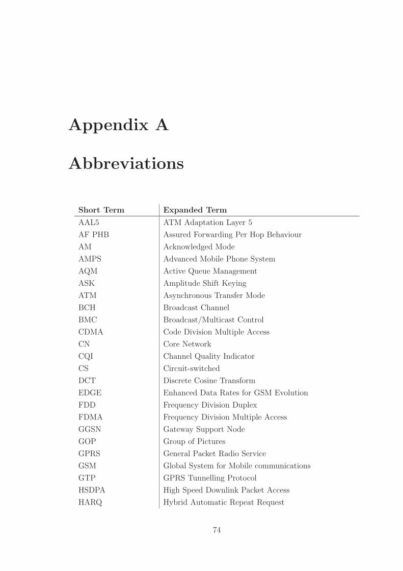
Appendix A
Abbreviations
Short Term Expanded Term
AAL5 ATM Adaptation Layer 5
AF PHB Assured Forwarding Per Hop Behaviour
AM Acknowledged Mode
AMPS Advanced Mobile Phone System
AQM Active Queue Management
ASK Amplitude Shift Keying
ATM Asynchronous Transfer Mode
BCH Broadcast Channel
BMC Broadcast/Multicast Control
CDMA Code Division Multiple Access
CN Core Network
CQI Channel Quality Indicator
CS Circuit-switched
DCT Discrete Cosine Transform
EDGE Enhanced Data Rates for GSM Evolution
FDD Frequency Division Duplex
FDMA Frequency Division Multiple Access
GGSN Gateway Support Node
GOP Group of Pictures
GPRS General Packet Radio Service
GSM Global System for Mobile communications
GTP GPRS Tunnelling Protocol
HSDPA High Speed Downlink Packet Access
HARQ Hybrid Automatic Repeat Request
74

IP Internet Protocol
ISDN Integrated Services Digital Network
JPEG Joint Photographic Experts Group
MAC Medium Access Control
MOS Mean Opinion Score
MPEG Moving Picture Experts Group
MRED Multi-level RED
MTU Maximum Transfer Unit
NMT Nordisk MobilTelefoni
OFDM Orthogonal frequency-division multiplexing
MC-CDMA Multi Carrier Code Division Multiple Access
PDCP Packet Data Convergence Protocol
PSK Phase Shift Keying
PPP Point-to-Point Protocol
PS Packet-switched
PSK Phase Shift Keying
PSNR Peak-Signal-To-Noise Ratio
PSTN Public switched telephone network
QAM Quadrature Amplitude Modulation
QoS Quality of Service
QPSK Quadrature PSK
RED Random Early Detection
RLC Radio Link Control
RNC Radio Network Controller
RRC Radio Resource Control
RTP Real-time Transport Protocol
SAW Stop and Wait
SDU Service Data Unit
SGSN Supporting GPRS Support Node
PDU Process Data Unit
PU Payload Units
TDD Time Division Duplex
TDMA Time Division Multiple Access
TM Transparent Mode
UDP User Datagram Protocol
UE User Equipment
UM Unacknowledged Mode
75

UMTS Universal Mobile Telecommunications System
UTRAN UMTS Radio Access Network
W-CDMA Wideband Code Division Multiple Access
3GPP Third Generation Partnership Project
76
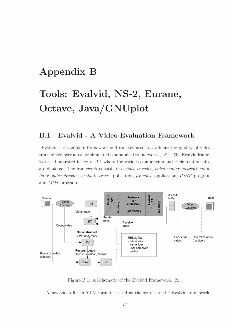
Appendix B
Tools: Evalvid, NS-2, Eurane,
Octave, Java/GNUplot
B.1 Evalvid - A Video Evaluation Framework
“Evalvid is a complete framework and tool-set used to evaluate the quality of video
transmitted over a real or simulated communication network”, [21]. The Evalvid frame-
work is illustrated in figure B.1 where the various components and their relationships
are depicted. The framework consists of a video encoder, video sender, network simu-
lator, video decoder, evaluate trace application, fix video application, PSNR program
and MOS program.
Figure B.1: A Schematic of the Evalvid Framework, [21].
A raw video file in YUV format is used as the source to the Evalvid framework.
77

A video encoder encodes this raw video file into a format suitable for streaming. For
simulations described as part of this thesis, the Xvid video encoder [54] was used to
encode a raw YUV file into MPEG4 format. The encoded video file is read by the Video
Sender which creates a video trace file and uses the trace file as input to the network
simulator. NS2 was the network simulator used. It was necessary to extend NS2 as
described in [23]. The extensions to NS2 were designed to read the video trace file and
from it generate sender and receiver trace files. These three trace files were required
to evaluate the quality of the video received by the end-user. After passing the video
trace file to NS2 the UMTS/HSDPA network simulation is performed and the resulting
sender and receiver trace files are generated. The video, sender and receiver trace files
are passed to the evaluate trace application which generates a possibly corrupt video
file as a result of the the simulated transmission over UMTS/HSDPA. The generated
video file is in the encoded MPEG4 format. The fix video application then decodes the
generated video file back into raw YUV format. The decoder used for this purpose was
provided by the FFmpeg application [55]. Using the peak-signal-to-noise (PSNR) and
mean opinion score (MOS) programs the end-to-end video quality can be evaluated.
Additional results are generated during the network simulation phase that include
jitter, delay, and loss rates.
B.2 Network Simulator 2
For simulations performed as part of this dissertation the NS-2 discrete event simulator
was used, [51]. NS-2 is an open source simulator targeted at networking research and
heavily used in the academic community. It provides good support for a variety of
wired and wireless network types.
NS-2 is written in two languages: C++ and OTcl. C++ is used where run-time
speeds and efficiency is required. OTcl is used as a front-end, where parameters or
configurations can easily be changed and tested. Each language supports its own class
hierarchy and classes belonging to each languages’ hierarchy are closely related to each
other. A user writes an OTcl script which is interpreted by the OTcl interpreter. The
OTcl interpreter creates new simulator object instances which are closely mirrored by
corresponding objects in the compiled hierarchy.
A network animator called NAM also comes as part of NS-2. NAM provides a
graphical illustration for viewing network simulations based on simulation results. Fig-
ure B.2 provides a simplistic view of the NS-2 simulator.
The standard NS-2 installation does not provide any support for UMTS or enhanced
UMTS (HSDPA) networks. To simulate these types of networks the Eurane plugin is
78

Figure B.2: Simplified view of the NS-2 simulator, [51].
required, (see section B.3). For further details about the NS-2 simulator see [51].
B.3 Eurane Plugin
Eurane is a plugin created for use with the NS-2 simulator for simulating third gener-
ation mobile telecommunications systems based on the release ’99 version of UMTS.
It implements the three functional nodes that make up the UMTS Terrestrial Radio
Access Network (UTRAN): the User Equipment (UE), the Base Station (BS) and the
Radio Node Controller (RNC). The RLC layer in the UMTS protocol architecture can
operate in either Acknowledged Mode (AM) or Unacknowledged Mode (UM). The UM
and AM entities in the simulation support most of the functions defined in the UMTS
standard. The physical layer has been implemented using a physical layer object that
is used to contain radio propagation models and compute a Channel Quality Indica-
tor (CQI) for each UE. The Eurane plugin has also been further enhanced to support
High Speed Downlink Packet Access (HSDPA). This further enhancement requires no
additional nodes, however additions to existing UMTS nodes have been included in the
form of a new MAC layer, MAC-hs. This layer includes most of the expected HSDPA
MAC layer functionality including fast scheduling and HARQ.
[50], [30] provide indepth details about the Eurane extension to NS-2 and describes
how to use it for creating simulations that model UMTS/HSDPA networks.
79
B.4 GNU Octave
“GNU Octave is a high-level language, primarily intended for numerical computations”,
[52]. An Octave preprocessing script has been created for generating input trace files.
The input trace files contain the received transmission and retransmission power values
and the corresponding CQI values for each TTI. This information is used to define the
channel characteristics for UEs in a Eurane/NS-2 simulation. The preprocessing script
uses a set of predefined user parameter values that can be changed to create an input
trace file with specific channel characteristics. Values for parameters such as the UE
multipath environment, speed, distance and transmission power are typical values that
can be set.
B.5 Java/GNUplot
“GNUplot is a portable command-line driven interactive data and function plotting
utility for UNIX, IBM OS/2, MS Windows, DOS, Macintosh, VMS, Atari and many
other platforms”, [53]. Gnuplot was used to create all the result graphs used in chapter
7. In order to create graphs using the GNUplot command-line utility a list of formatted
values must be passed to the GNUplot utility. The values were parsed and formatted
from results obtained from simulations using a Java utility created especially for this
purpose. The Java utility included functions for parsing, extracting and calculating
values for PSNR, MOS, end-to-end delay and average packet size.
80

Bibliography
[1] Guo, Y.J., Advances in Mobile Radio Access Networks, Artech House, 2004
[2] Harri Holma and Antti Toskala, WCDMA For UTMS, Wiley, 2nd Edition.
[3] Jochen Schiller, Mobile Communications, 2000 Addison-Wesley, 2nd Edition.
[4] Pablo Jose and Ameigeiras Gutierrez, Packet Scheduling and Quality of Service
in HSDPA, Ph. D. Thesis, October 2003, Dept of Communication Technology,
Institute of Electronic Systems, Aalborg University.
[5] Andy Craigen, The role and impact of user equipment in HSxPA networks,
Icera Inc., White paper, Doc Number: WHP 005, Version: 1.0.
[6] Aun Haider, Richard Harris, A Novel Proportional Fair Scheduling Algorithm
for HSDPA in UMTS Networks, 2nd International Conference on Wireless
Broadband and Ultra Wideband Communications (AusWireless 2007).
[7] K Singh, J Orozco, D Ros, G Rubino, Streaming of H.264 Video over HSDPA:
Impact of MAC-Layer Schedulers on User-Perceived Quality, Collection des
rapports de Recherche de l’ENST Bretagne 2007.
[8] John G. Apostolopoulos, Wai- tian Tan, Susie J. Wee, Mobile and Media Sys-
tems Laboratory, HP Laboratories Palo Alto, Video Streaming: Concepts,
Algorithms, and Systems, September 2002
[9] G. K. Wallace, The JPEG Still Picture Compression Standard, Communica-
tions of the ACM, April, 1991.
[10] ITU-T BT.601 Recommendation: Studio encoding parameters of dig-
ital television for standard 4:3 and wide screen 16:9 aspect ratios,
http://www.itu.int/rec/R-REC-BT.601/en
[11] Lee, S., Spread Spectrum CDMA: IS-95 and IS-2000 for RF Communications,
McGraw-Hill Professional 2002
81
[12] 3GPP2 C.S0001-D, 3rd Generation Partnership Project 2, Introduction to
cdma2000 Standards for Spread Spectrum Systems, Release D, Version 2.0,
September 2005
[13] Overview of 3GPP Release 5 Summary of all Release 5 Features, ETSI Mobile
Competence Centre, Version 9th September 2003
[14] 3GPP TS 25.401, 3rd Generation Partnership Project; Technical Specification
Group Radio Access Network; UTRAN overall description
[15] 3GPP TS 25.322, 3rd Generation Partnership Project; Technical Specification
Group Radio Access Network; Radio Link Control (RLC) protocol specification
[16] 3GPP TS 25.321, 3rd Generation Partnership Project; Technical Specification
Group Radio Access Network; Medium Access Control (MAC) protocol speci-
fication
[17] 3GPP TS 25.301, 3rd Generation Partnership Project; Technical Specification
Group Radio Access Network; Radio Interface Protocol Architecture
[18] 3GPP TS 25.323, 3rd Generation Partnership Project; Technical Specification
Group Radio Access Network; Packet Data Convergence Protocol (PDCP)
specification
[19] 3GPP TS 25.324, 3rd Generation Partnership Project; Technical Specification
Group Radio Access Network; Broadcast/Multicast Control (BMC) specifica-
tion
[20] 3GPP TS 25.308, 3rd Generation Partnership Project; Technical Specification
Group Radio Access Network; High Speed Downlink Packet Access (HSDPA)
Overall description
[21] Jirka Klaue, Berthold Rathke, Adam Wolisz, Evalvid - A Framework for Video
Transmission and Quality Evaluation, Proc. of the 13th International Confer-
ence on Modelling Techniques and Tools for Computer Performance Evaluation,
pp. 255-272, Urbana, Illinois, USA, September 2003
[22] J. Klaue, B. Rathke, and A. Wolisz, EvalVid - A Video Quality Evaluation
Tool-set, http://www.tkn.tu-berlin.de/research/evalvid
[23] Chih-Heng Ke, Ce-Kuen Shieh, Wen-Shyang Hwang, Artur Ziviani,
An Evaluation Framework for More Realistic Simulations of MPEG
82

Video Transmission, Journal of Information Science and Engineering,
http://hpds.ee.ncku.edu.tw/smallko/ns2/Evalvid in NS2.htm
[24] B. Walke, P. SEIDENBERG, M. P. Althoff, UTMS: The Fundamentals, 2003
John Wiley and Sons, Ltd.
[25] S. Blake, D. Black, M. Carlson, E. Davies, Z. Wang, and W. Weiss, An archi-
tecture for differentiated services, Internet Standards Track RFC 2475, IETF,
Dec. 1998.
[26] S. Floyd, V. Jacobson, Random early detection gateways for congestion avoid-
ance, IEEE/ACM Transactions on Networking, vol. 1, no.4, pp. 397-413, Aug.
1993.
[27] Makkar, R. and Lambadaris, I. and Salim, JH and Seddigh, N. and Nandy,
B. and Babiarz, J., Empirical study of buffer management scheme for Diff-
serv assured forwarding PHB, Proceedings. Ninth International Conference on
Computer Communications and Networks, pp. 632-637, 2000
[28] Heinanen, J. and Baker, F. and Weiss, W. and Wroclawski, J., Assured For-
warding PHB Group, Internet Standards Track RFC 2597, June 1999
[29] Gross, J. and Klaue, J. and Karl, H. and Wolisz, A., Cross-Layer Optimiza-
tion of OFDM Transmission Systems for MPEG-4 Video Streaming, Computer
Communications, vol. 27, no. 11, pp. 1044-1055, 2004 Elsevier
[30] N. Whillans, I. de Bruin, S. Oosthoek, F. Brouwer, A. Jehangir, G. Heijenk,
Seacorn project, deliverable D3.2v2, End-to-end network model for Enhanced
UMTS, Oct. 2003
[31] Haug, T., A commentary on standardization practices: lessons from the NMT
and GSM mobile telephone standards histories, Telecommunications Policy,
vol. 26, no. 3-4, pp. 101-107, 2002 Elsevier
[32] W. Rae Young, AMPS: Introduction, Background, and Objectives, Bell System
Technical Journal, vol. 58, 1, pp 1-14, January 1979.
[33] Review Of Frequency Allocations For Cordless Telephones,
http://www.ofta.gov.hk/en/ad-comm/rsac/paper/rsac6-2002.pdf, RSAC
Paper, June 2002
83

[34] Steele, R., The evolution of personal communications, Personal Communica-
tions, IEEE Wireless Communications, vol. 1, no. 2, 1994
[35] Nicopolitidis, P. and Obaidat, MS and Papadimitriou, GI and Pomportsis, AS,
Wireless networks, 2003 J. Wiley Hoboken, NJ
[36] Goodman, DJ, Trends in cellular and cordless communications, Communica-
tions Magazine, IEEE, vol. 29, no. 6, pp. 31-40, 1991
[37] Halonen, T. and Melero, J., GSM, GPRS and EDGE Performance: Evolution
Towards 3G/UMTS, 2003 Wiley
[38] Gazis, V. and Houssos, N. and Alonistioti, A. and Merakos, L., Evolving per-
spectives of 4th generation mobile communication systems, Personal, Indoor
and Mobile Radio Communications, 2002. The 13th IEEE International Sym-
posium on, vol. 1, 2002
[39] Farrokh, A. and Krishnamurthy, V., Opportunistic scheduling for streaming
multimedia users in high-speed downlink packet access (HSDPA), journal:
IEEE Transactions on Multimedia, vol. 8, no. 4, pp. 844-855, 2006
[40] Bharathi Athinarayanan, Anritsu Corporation, India, http://www.aubraux.
com/articles/hsdpa-high-speed-downlink-packet-access.php?page=2
[41] M. Wilson, Streaming Media, http://www.public.iastate.edu/mawilson/501
/home.shtml
[42] ITU-T Recommendation H.264, Nov. 2007, http://www.itu.int/rec/
dologin pub.asp?lang=e&id=T-REC-H.264-200711-I!!PDF-E&type=items
[43] Windows Media Developer Center, About YUV Video,
http://msdn.microsoft.com/en-us/library/bb530104(VS.85).aspx
[44] Devendra Sharma, Introduction to High speed downlink packet access (HS-
DPA), http://www.3g4g.co.uk/Tutorial/DS/ds hsdpa.html.
[45] Forbes.com, http://www.forbes.com/personaltech/2007/10/25/mobile-market
-subscription-technology-personaltech-cz 1025mobilemap.html.
[46] CellularOnline, http://www.cellular.co.za/technologies/3g/3g.htm.
[47] 3G4G Wireless Resource Center, http://www.3g4g.co.uk/4G/faq.html.
84

[48] ITU-T Recommendations, http://www.itu.int/rec/T-REC-H/e
[49] ISO Standards, http://www.iso.org/iso/iso catalogue.htm
[50] EURANE, http://eurane.ti-wmc.nl/eurane/
[51] NS-2 Discrete Event Simulator, http://nsnam.isi.edu/nsnam/index.php/Main Page
[52] GNU Octave, version 2.9.12, http://www.gnu.org/software/octave/
[53] Gnuplot, version 4.2, http://www.gnuplot.info/
[54] Xvid, version 1.1.3, http://www.xvid.org/
[55] FFMpeg, http://ffmpeg.mplayerhq.hu/
[56] European Telecommunications Standards Institute, http://www.etsi.org
/WebSite/homepage.aspx
85