QM Lecture Notes B.R.P. Gamage
5
Graduate Quantum Mechanics II 1 TimeDependent Perturbation theory continued For a Hamiltonian ! = ℎ ! !!"# we can write, ! = ℎ ! ℏ !(! !" !! ! )! ! ! ! which leads to the probability of going from → : → ; = ℎ ! ! ℏ ! sin !" − 2 !" − 2 ! ! This is under the assumption that the system is in state | at = 0. Otherwise, we have to replace t with (t–t 0 ) Assume we prepare | ! = − ! ! What is → = ! ! ? Simply replace t with For large → ∞ we can use Fermi’s golden rule ! ! = !! ℏ ! ! ! − ! − ℏ ! , meaning we have a constant rate of transition per unit time. How can we get these two contradictory results to agree for the same situation? Note: Fermi’s Golden Rule can only work if either the final state energy or the frequency distribution of the perturbing Hamiltonian are continuous functions – otherwise the deltafunction will make no sense. So let’s study the case where the final state wave function is an eigenstate to the momentum operator (and therefore the unperturbed Hamiltonian H 0 is the free particle Hamiltonian). What is the probability to find the momentum somewhere in a small volume of momentum space? (∆ ! ) = Ψ ! ∆ ! Where ∆ ! = ! ∆∆Ω So we need to find the overlap ! ! = Ψ ! and multiply by the volume space. → + ∆ ! = ! ! ′ ! ! ! ! !! ! ! ! !! ! Ω ∆! = ΔΩ ! ! ′ ! ! ! ! !! ! ! ! !! ! Since we are integrating over a very small volume,
Transcript of QM Lecture Notes B.R.P. Gamage

Graduate Quantum Mechanics II
1
Time-‐Dependent Perturbation theory continued
For a Hamiltonian 𝐻! 𝑡 = ℎ!𝑒!!"# we can write,
𝑑! 𝑡 =𝑓 ℎ! 𝑖𝑖ℏ
𝑒!(!!"!!!)!! 𝑑𝑡!
!
which leads to the probability of going from 𝑖 → 𝑓 :
𝑃 𝑖 → 𝑓; 𝑡 =𝑓 ℎ! 𝑖
!
ℏ!sin 𝜔!" − 𝜔 𝑡
2𝜔!" − 𝜔 𝑡
2
!
𝑡!
This is under the assumption that the system is in state |𝑖 at 𝑡 = 0. Otherwise, we have to replace t with (t – t0)
Assume we prepare |𝑖 𝑎𝑡 𝑡! = − !!
What is 𝑃 𝑖 → 𝑓 𝑎𝑡 𝑡 = !! ? Simply replace t with 𝜏
For large 𝜏 → ∞ we can use Fermi’s golden rule
𝑑!! = !!
ℏ𝑓 𝐻! 𝑖
! 𝜏 𝛿 𝐸! − 𝐸! − ℏ𝜔! , meaning we have a constant rate of transition per unit time.
How can we get these two contradictory results to agree for the same situation?
Note: Fermi’s Golden Rule can only work if either the final state energy or the frequency distribution of the perturbing Hamiltonian are continuous functions – otherwise the delta-‐function will make no sense.
So let’s study the case where the final state wave function is an eigenstate to the momentum operator (and therefore the unperturbed Hamiltonian H0 is the free particle Hamiltonian). What is the probability to find the momentum somewhere in a small volume of momentum space?
𝑃(∆!𝑝) = 𝑃 Ψ!∆!𝑝 Where ∆!𝑝 = 𝑝!∆𝑝∆Ω
So we need to find the overlap 𝑑!! = 𝑃 Ψ
! and multiply by the volume space.
𝑃 𝑖 → 𝑃 + ∆!𝑝 = 𝑑!!𝑃′!𝑑𝑃!
!!!!!
!!!!!
𝑑Ω∆!
= ΔΩ 𝑑!!𝑃′!𝑑𝑃!
!!!!!
!!!!!
Since we are integrating over a very small volume,

Graduate Quantum Mechanics II
2
𝑃 𝑖 → 𝑃 + ∆!𝑝 = ΔΩ 𝑃 𝑑!!𝑃′𝑑𝑃!
!!!!!
!!!!!
Applying what we got earlier for 𝑑!! in this equation,
𝑃 𝑖 → 𝑓 = ΔΩ 𝑚𝑃! 2𝜋ℏ
𝑓 𝐻! 𝑖! 𝑇 𝛿 𝐸! − 𝐸! − ℏ𝜔! 𝑑
𝑃!!
2𝑚
!!!!!
!!!!!
The only variable that depends on 𝑃! is,
𝐸! =𝑃′!
2𝑚
And the integral becomes,
𝛿 𝐸! − 𝐸! − ℏ𝜔! 𝑑𝐸!
!(!!!!! )
!(!!!!! )
= 1 ; 𝐼𝑓 𝑡ℎ𝑒 𝑣𝑎𝑙𝑢𝑒 𝑖𝑠 𝑖𝑛𝑠𝑖𝑑𝑒 𝑡ℎ𝑒 𝑙𝑖𝑚𝑖𝑡0 ; 𝑖𝑓 𝑖𝑡 𝑖𝑠 𝑛𝑜𝑡 𝑖𝑛𝑠𝑖𝑑𝑒 𝑡ℎ𝑒 𝑙𝑖𝑚𝑖𝑡
The final solution then becomes,
𝑃 𝑖 → 𝑓 = ΔΩ m𝑃! 2𝜋ℏ
𝑓 𝐻! 𝑖! 𝑇
But what about the other equation ? how are we going to integrate it to get a solution closer to this one?
𝑃 𝑖 → 𝑓 =𝑓 𝐻! 𝑖
!
ℏ!ΔΩ
sin 𝜔!" − 𝜔 𝑡2
𝜔!" − 𝜔 𝑡2
!
𝑡!𝑃′!𝑑𝑃!!!!!!
!!!!!
Where,
𝜔!" =𝐸!ℏ−𝐸!ℏ=
𝑃!!
2𝑚ℏ−𝐸!ℏ
If 𝜔!" − 𝜔 𝑡 < 𝜋
Sine of a small number divided by that small number is one. So,
Graduate Quantum Mechanics II
3
𝑃 𝑖 → 𝑓 =𝑓 𝐻! 𝑖
!
ℏ!ΔΩ𝑃!!∆P t!
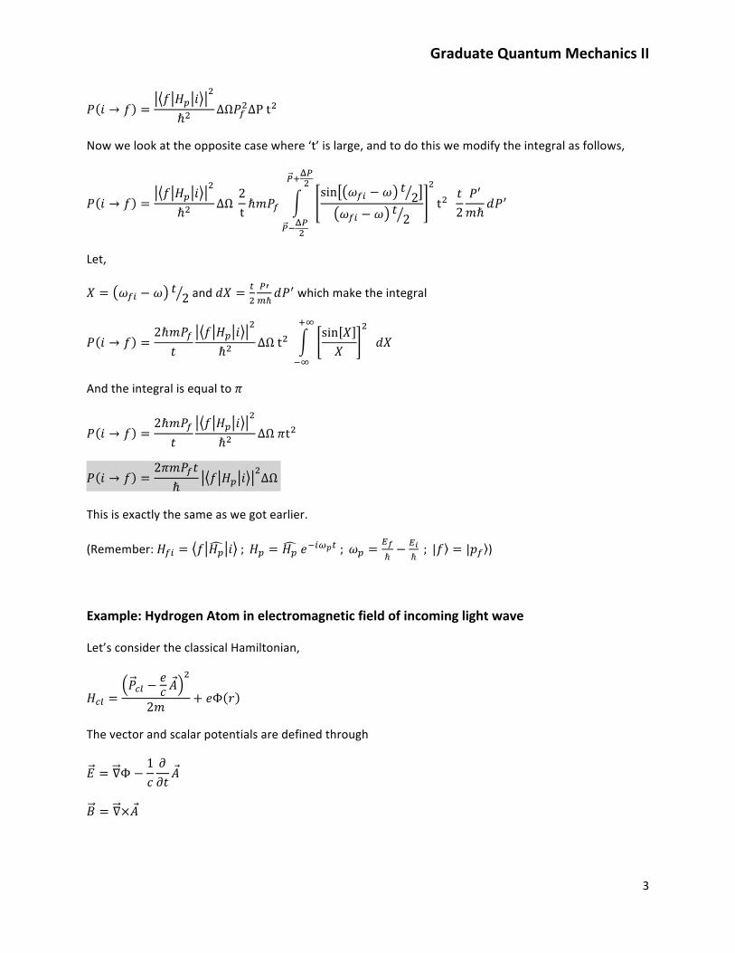
Now we look at the opposite case where ‘t’ is large, and to do this we modify the integral as follows,
𝑃 𝑖 → 𝑓 =𝑓 𝐻! 𝑖
!
ℏ!ΔΩ
2tℏ𝑚𝑃!
sin 𝜔!" − 𝜔 𝑡2
𝜔!" − 𝜔 𝑡2
!
t! 𝑡2𝑃′𝑚ℏ
𝑑𝑃!!!!!!
!!!!!
Let,
𝑋 = 𝜔!" − 𝜔 𝑡2 and 𝑑𝑋 =
!!!!!ℏ𝑑𝑃! which make the integral
𝑃 𝑖 → 𝑓 =2ℏ𝑚𝑃!𝑡
𝑓 𝐻! 𝑖!
ℏ!ΔΩ t!
sin 𝑋𝑋
!
𝑑𝑋!!
!!
And the integral is equal to 𝜋
𝑃 𝑖 → 𝑓 =2ℏ𝑚𝑃!𝑡
𝑓 𝐻! 𝑖!
ℏ!ΔΩ 𝜋t!
𝑃 𝑖 → 𝑓 =2𝜋𝑚𝑃!𝑡
ℏ𝑓 𝐻! 𝑖
!ΔΩ
This is exactly the same as we got earlier.
(Remember: 𝐻!" = 𝑓 𝐻! 𝑖 ; 𝐻! = 𝐻! 𝑒!!!!! ; 𝜔! =!!ℏ− !!
ℏ ; |𝑓 = |𝑝! )
Example: Hydrogen Atom in electromagnetic field of incoming light wave
Let’s consider the classical Hamiltonian,
𝐻!" =𝑃!" −
𝑒𝑐 𝐴
!
2𝑚+ 𝑒Φ 𝑟
The vector and scalar potentials are defined through
𝐸 = ∇Φ −1𝑐𝜕𝜕𝑡𝐴
𝐵 = ∇×𝐴

Graduate Quantum Mechanics II
4
Maxwell’s equations then become (the other two are automatically fulfilled due to the definition)
∇!Φ +1𝑐𝜕𝜕𝑡
∇ ∙ 𝐴 = −4𝜋𝜌
∇!𝐴 −1𝑐!
𝜕!
𝜕𝑡!𝐴 − ∇ ∇𝐴 +
1𝑐𝜕𝜕𝑡Φ = −
4𝜋𝚥𝑐
For free space no charge or current, so 𝜌 = 𝚥 = 0
From the previous semester,
Gauge transformation,
Φ → Φ! = Φ +1𝑐𝜕𝜕𝑡Λ
𝐴 → 𝐴! = 𝐴 − ∇Λ
leaves all the physical observables (electric and magnetic field) unchanged. We can therefore adopt additional requirements on the potentials. In particular, in the absence of charges and currents, we can use the Coulomb Gauge:
∇𝐴 = 0 ; Φ = 0
So using the only remaining non-‐trivial equation above,
∇!𝐴 −1𝑐!
𝜕!
𝜕𝑡!𝐴 = 0
Which has a solution like,
𝐴 𝑟, 𝑡 = 𝐴! cos 𝑘 ∙ 𝑟 − 𝜔𝑡 =12𝐴! 𝑒! !∙!!!" + 𝑒!! !∙!!!"
For this solution to satisfy the above equation,
𝑘! −𝜔!
𝑐!= 0 → 𝑘 =
𝜔𝑐
𝐴 ∙ 𝑘 = 0 (Coulomb Gauge)
To find the electric field, using equation one,
𝐸 = ∇Φ −1𝑐𝜕𝜕𝑡𝐴

Graduate Quantum Mechanics II
5
𝐸 =𝜔𝑐𝐴! sin 𝑘 ∙ 𝑟 − 𝜔𝑡
And,
𝐵 = 𝑘×𝐴! sin 𝑘 ∙ 𝑟 − 𝜔𝑡 = 𝑘×𝐸
Using the classical Hamiltonian we now write the quantum-‐mechanical Hamilton operator for the wave
𝐻! =𝑃!
2𝑚−
𝑒2𝑚𝑐
𝑃 ∙ 𝐴 + 𝐴 ∙ 𝑃 +𝐴!
2𝑚𝑐!−𝑒!
𝑟
(the potential due to the nucleus is of course non-‐zero; only the one from the incoming wave is).
If we apply this to any wave function
ℏ!∇ ∙ 𝐴 Ψ 𝑥 = ℏ
!𝐴 ∙ ∇ Ψ 𝑥 (because of the Coulomb Gauge condition)
So
𝑃 ∙ 𝐴 = 𝐴 ∙ 𝑃
Now we write the total Hamiltonian including the electrostatic field from the nucleus
𝐻 =𝑃!
2𝑚−
𝑒2𝑚𝑐
𝑃 ∙ 𝐴 + 𝐴 ∙ 𝑃 +𝐴!
2𝑚𝑐!−𝑒!
𝑟= 𝐻! + 𝐻!
𝐻! =!
!!"𝐴! ∙ 𝑃 𝑒! !∙!!!" (we leave out the 𝑒!! !∙!!!" term since it cannot fulfill the requirement of
the delta-‐function in Fermi’s Golden Rule).
By comparing this with,
𝐻! = 𝐻! 𝑒!!!!!
We can get,
𝐻! =𝑒
2𝑚𝑐𝐴! ∙ 𝑃 𝑒! !∙!
In the integral, r will be of order a0. Furthermore, for a photon of a few times 10 eV (which is what we
need to eject the electron), k is of order 0.1 nm-‐1 and a0 = 0.05 nm. Therefore, we can take 𝑘 ∙ 𝑟~0.