QCD and Jets - UC Davis Particle Theory:...
53
March 10, 2006 10:58 Proceedings Trim Size: 9in x 6in qcd˙jets 1 QCD and Jets George Sterman C.N. Yang Institute for Theoretical Physics, Stony Brook University, SUNY Stony Brook, New York 11794-3840, U.S.A. These lectures introduce some of the basic methods of perturbative QCD and their applications to phenomenology at high energy. Emphasis is given to techniques that are used to study QCD and related field theories to all orders in perturbation theory, with introductions to infrared safety, factorization and evolution in high energy hard scattering. 1. Introduction Quantum chromodynamics is the component of the Standard Model that describes the strong interactions. It is a theory formulated in terms of quarks and gluons at the Lagrangian level, but observed in terms of nucleons and mesons in nature. Partly because of this, its verification required formulating new methods and asking new questions on how to confront quantum field theories with experiment, especially those that exhibit strong coupling. In what might seem an almost paradoxical outcome, new roles were recognized for perturbative methods based on the elementary constituents of the theory. Since strong coupling is a feature of many extensions of the Standard Model and of string theories, these theoretical developments in perturbative QCD remain of interest in a more general context. In addition, the perturbative analysis of hadronic scattering and final states played an essential role in the verification of the electroweak sector of the Standard Model, through the discoveries of the W and Z bosons and of the bottom and top quarks. Likewise, perturbative methods are indispensable in the search for new physics at all colliders, which will keep them relevant to phenomenology for the foreseeable future. Finally, at lower but still substantial energies, new capabilities to study the polarization-dependence of hadronic scattering and the strong interactions at high temperatures and densities are opening new avenues for the study of quantum field theory. These lectures, of course, cannot cover the full range of QCD, even at high energies in perturbation theory. They are meant to be an introduction for students familiar with the basics of quantum field theory and the Standard Model, but not with applications of perturbative QCD. I will emphasize the formulation and calcu- lation of observables using perturbative methods, and discuss the justification of perturbative calculations in a theory like QCD, with esssentially nonperturbative long-distance behavior. I will also introduce elements of the phenomenology of perturbative QCD at high energies, keeping in mind its use in the search for signals of new physics. 2. QCD from Asymptotic Freedom to Infrared Safety We begin with a quick prehistory of quantum chromodynamics, and of the strands of experiment and theory that converged in the concept of asymptotic freedom. We also show how infrared safety makes possible a wide range of phenomenological implementations of asymptotic freedom.
-
Upload
nguyenhuong -
Category
Documents
-
view
213 -
download
0
Transcript of QCD and Jets - UC Davis Particle Theory:...

March 10, 2006 10:58 Proceedings Trim Size: 9in x 6in qcd˙jets
1
QCD and Jets
George Sterman
C.N. Yang Institute for Theoretical Physics, Stony Brook University, SUNY
Stony Brook, New York 11794-3840, U.S.A.
These lectures introduce some of the basic methods of perturbative QCD and theirapplications to phenomenology at high energy. Emphasis is given to techniquesthat are used to study QCD and related field theories to all orders in perturbationtheory, with introductions to infrared safety, factorization and evolution in highenergy hard scattering.
1. Introduction
Quantum chromodynamics is the component of the Standard Model that describes the strong interactions. It is
a theory formulated in terms of quarks and gluons at the Lagrangian level, but observed in terms of nucleons
and mesons in nature. Partly because of this, its verification required formulating new methods and asking new
questions on how to confront quantum field theories with experiment, especially those that exhibit strong coupling.
In what might seem an almost paradoxical outcome, new roles were recognized for perturbative methods based
on the elementary constituents of the theory.
Since strong coupling is a feature of many extensions of the Standard Model and of string theories, these
theoretical developments in perturbative QCD remain of interest in a more general context. In addition, the
perturbative analysis of hadronic scattering and final states played an essential role in the verification of the
electroweak sector of the Standard Model, through the discoveries of the W and Z bosons and of the bottom
and top quarks. Likewise, perturbative methods are indispensable in the search for new physics at all colliders,
which will keep them relevant to phenomenology for the foreseeable future. Finally, at lower but still substantial
energies, new capabilities to study the polarization-dependence of hadronic scattering and the strong interactions
at high temperatures and densities are opening new avenues for the study of quantum field theory.
These lectures, of course, cannot cover the full range of QCD, even at high energies in perturbation theory.
They are meant to be an introduction for students familiar with the basics of quantum field theory and the
Standard Model, but not with applications of perturbative QCD. I will emphasize the formulation and calcu-
lation of observables using perturbative methods, and discuss the justification of perturbative calculations in a
theory like QCD, with esssentially nonperturbative long-distance behavior. I will also introduce elements of the
phenomenology of perturbative QCD at high energies, keeping in mind its use in the search for signals of new
physics.
2. QCD from Asymptotic Freedom to Infrared Safety
We begin with a quick prehistory of quantum chromodynamics, and of the strands of experiment and theory that
converged in the concept of asymptotic freedom. We also show how infrared safety makes possible a wide range
of phenomenological implementations of asymptotic freedom.

March 10, 2006 10:58 Proceedings Trim Size: 9in x 6in qcd˙jets
2
2.1. Why QCD?
The search that culminated in the SU(3) gauge theory quantum chromodynamics was triggered by the discovery of
an ever-growing list of hadronic states, including mesons, excited nucleons and a variety of resonances, beginning
with the ∆ resonances first seen in the early 1950s 1, and continuing to this day 2. Already in 1949, the idea was
put forward that mesons might be composites of more elementary states (of nucleons in the very early work of
Fermi and Yang 3). Clearly hadrons were not themselves elementary in the normal sense, but for a long time the
strong couplings between hadronic states, and their ever-growing number, left the situation unsettled.
In broad terms, two alternative viewpoints were entertained for nucleon and other hadronic states. In bootstrap
scenarios, each hadronic state was at once deducible from the others, yet irreducible, in the sense that no hadronic
state was more elementary than any other. This idea eventually evolved through the dual model 4 into string
theory, leaving the strong interactions behind, at least temporarily. The more conservative viewpoint regarded
hadrons as composite states of elementary particles, but the observed couplings seemed to pose an insurmountable
barrier to a field-theoretic treatment. Still, the growing success of quantum electrodynamics held out at least the
possibility that such a picture might somehow emerge.
With the weak and electromagnetic interactions serving as diagnostics, what we now call flavor symmetry
was developed out of the spectroscopy of hadronic states. Their interactions through local currents also hinted
at point-like substructure. The weak and electromagnetic currents, in their turn, were naturally described as
coupling to fundamental objects, and the quark model was born, partly as a wonderfully compact classification
scheme, and partly as a dynamical model of hadrons.
Increases in accelerator energies eventually clarified the situation. A prologue, both scientifically and techno-
logically, were the 1950’s measurements of electron-proton elastic scattering 5. Imposing the relevant symmetries
of the electromagnetic and strong interactions (parity and time-reversal invariance), the cross section for electron-
nucleon unpolarized scattering at fixed angle is customarily expressed in the nucleon rest frame, as
dσ
dΩe=
[
α2EM cos2(θ/2)
4E2 sin4(θ/2)
]
E′
E
( |GE(Q)|2 + τ |GM (Q)|21 + τ
+ 2τ |GM (Q)|2 tan2 θ/2
)
. (1)
The term in square brackets is the (Mott) cross section for the scattering of a relativistic electron of energy E by
a fixed source of unit charge, while E′ is the outgoing electron energy. The variable τ ≡ Q2/4M2N , with MN the
nucleon mass and Q2 = −EE′ sin2(θ/2) the invariant momentum transfer. The functions GE(Q) and GM (Q) are
the electric and magnetic form factors. They fall off rapidly with momentum transfer, roughly as
|G(Q)i| ∼1
(1 + Q2/µ20)
2, (2)
where µ0 ∼ 0.7GeV . This simple behavior is anaolgous to the form factors of nonrelativistic bound states with
extended charge distributions 6. This suggests a substructure for the nucleon, but leaves its nature mysterious.
Indeed, much is still being learned about nucleon form factors 7 and their relation to the quarks and gluons of
QCD 8,9. The experiments are difficult, however, because of the form factors’ rapid decrease with Q. This is
simply to say that when a proton is hit hard, it is likely to radiate or to break apart.
As available electron energies increased it became possible by the late 1960’s to go far beyond elastic scattering,
and to study highly (“deep”) inelastic reactions. In these experiments, nature’s choice became manifest.
The idea is simple, and analogous in many ways to the famous Rutherford experiments that revealed the
atomic nucleus. A high energy electron beam is made to collide with a nucleon target. One observes the recoil of
the electron, measuring the total cross section as a function of transfered energy and scattering angle, as indicated
in Fig. 1. Although each individual event is generally quite complicated, a simpler pattern emerges when events
at a given momentum transfer are grouped together. Imposing again the relevant symmetries, a general deep-
inelastic scattering (DIS) cross section can be written in terms of dimensionless structure functions, F1(x, Q2)

March 10, 2006 10:58 Proceedings Trim Size: 9in x 6in qcd˙jets
3
and F2(x, Q2), where the variable x is defined as
x =Q2
2pN · q , (3)
with q, q2 = −Q2, the momentum transfer as above. In these terms, the cross section (again in the nucleon rest
frame) is analogous to the one for elastic scattering,
dσ
dE′ dΩ=
[
α2EM
2SE sin4(θ/2)
] (
2 sin2(θ/2)F1(x, Q2) + cos2(θ/2)m
E − E′F2(x, Q2)
)
, (4)
where S is the overall center of mass energy squared. The factor in square brackets is again proportional to the
cross section for scattering from a point charge by single-photon exchange. The complexities due to the hadron
target are all in the structure functions. The structure functions, however, turn out to be simpler than might
have been expected. To a good approximation in the original experiments, the F ’s were found to be indpendent
of momentum transfer. This surprising result, called scaling, was in contrast to the rapid decrease of elastic form
factors.
->
θ
** **
**
Doesn't matter much.
Same as:
θ->
Figure 1. Picture of deep-inelastic scattering
It is as if, for the purposes of inclusive scattering, the Q-dependence is given entirely by the elastic scattering of
an electron from a point charge. Representing these point charges by ? as in the figure, we can write schematically,
σeN→eX(x, Q) ∼ σ(elastic)e?→e? (x, Q) × FN (x) , (5)
where FN is a linear combination of the structure functions and where σ(elastic)e?→e? (x, Q) is the lowest-order cross
section for the scattering of an electron on an elementary ?, with x given by (3). The precise cross section depends
on the spin of the ?’s, which are identified as the charged partons inside the proton 10. The variable x can then be
given a nice physical interpretation, if we think of the scattering in a frame where the nucleon and all its partons
are moving in the same direction at velocities approaching the speed of light, the eN center of mass frame for
example. In this frame, if the nucleon momentum is pN , the parton’s momentum should be some fraction of that,

March 10, 2006 10:58 Proceedings Trim Size: 9in x 6in qcd˙jets
4
call it ξpN , with 0 < ξ < 1. Then if the scattered parton ? is to be on-shell, and and if we neglect its mass in the
kinematics of the hard scattering, we find
(ξpN + q)2 = 0 → ξ =Q2
2pN · q = x . (6)
Thus the scaling variable x observed in a specific event is the momentum fraction of the parton from which the
electron has scattered.
We can now interpret the x-dependent structure functions for DIS as probabilities to find partons with definite
momentum fractions,
σeN→eX(x, Q) ∼ σ(elastic)e?→e? (x, Q) × (probability to a find parton) . (7)
The precise form of the parton-electron cross section depends on the spin of the parton through the structure
functions. In this way, early experiments could already identify the spin as 1/2, and the partons quickly became
identified with quarks.
The parton model gave an appealing physical picture of the early deep-inelastic scattering experiments, but
it seemed to contradict other experimental facts. If the cross section can be computed with lowest-order electro-
magnetic scattering, then partons must in some sense be weakly bound. But then what happened to the strong
force? Already at that time searches for free quarks had come up empty, and the concept of quark confinement
was taken as yet another sign of the strength of nucleon’s binding. How was it possible to describe such a force,
strong enough to confine yet weak enough for scaling?
2.2. Quantum chromodynamics and asymptotic freedom
Scaling posed the question to which QCD was the answer. The essential feature of QCD is asymptotic freedom11, according to which its coupling, gs decreases toward short distances and increases toward longer distances and
times. Asymptotic freedom matches qualitatively with the requirements of approximate scaling, and its converse,
that the coupling increases toward longer distances and times, is consistent with the behavior that gave the
strong force its name. As we shall see, asymptotic freedom also provides systematic and quantitative predictions
for corrections to scaling. Let’s recall first how the strength of a coupling varies with distance scale.
The (classical) Lagrangian of QCD is 12
L =
nf∑
f=1
qf (i/∂ − gs/A + mf ) qf − 1
2Tr(F 2
µν [A]) , (8)
in terms of nf flavors of quark fields and SU(3) gluon fields Aµ =∑8
a=1 AµaTa, with Ta the generators of SU(3)
in the fundamental representation. The field strengths Fµν [A] = ∂µAν − ∂νAµ + igs[Aµ, Aν ] specify the familiar
three- and four-point gluon couplings of nonabelian gauge theory 13. We will not need their explicit forms here.
This Lagrangian, with its exact color gauge symmetries, also inherited the approximate flavor symmetries of the
quark models, and was automatically consistent with properties and consequences of hadronic weak interactions
that follow from an analysis of vector and axial vector currents 14. In addition to the right currents, QCD had
just the right kind of forces.
A simple picture (if not particularly convenient for calculation) of the scale dependence of the coupling is
shown in Fig. 2, which represents the perturbative series for the amplitude for fermion-vector coupling. We imagine
computing this quantity in coordinate space, which amounts to integrating over the positions of vertices. At lowest
order, this amplitude is just the coupling (e in QED, gs for QCD, etc.). At the one-loop level, the amplitude
requires renormalization because whenever two vertices, say at x and y, coincide, a propagator connecting them
diverges. For example, the coordinate space propagator for a massless boson is
1
(2π)21
(x − y)2 − iε= i
∫
d4k
(2π)4e−ik·(x−y) 1
k2 + iε. (9)

March 10, 2006 10:58 Proceedings Trim Size: 9in x 6in qcd˙jets
5
Alternatively, we can just notice that the integrals over the positions of the vertices are dimensionless in gauge
theories. Such integrals have no choice but to diverge for ultraviolet momenta, where masses are negligible.
In these terms, the renormalized coupling may be defined (in Euclidean space) as the sum of all diagrams with
vertices contained within a four-dimensional sphere of diameter cT , with c the speed of light and T any fixed
time. Let’s call the coupling defined this way gs(h/T ), where h/T is the corresponding energy scale, which is then
the renormalization scale. Although we cannot compute gs(h/T ) directly, we can compute the right-hand side of
the equation
Td
dTgs(h/T ) =
b0
16π2g3
s(h/T ) + · · · , (10)
where the term shown on the right is the finite result found when one of the vertices is fixed at the edge of the
sphere. (We shall neglect higher orders, assuming that gs is small.) In effect, the divergent part of the integrals is
independent of T . The constant b0, of course, depends on the theory. For QCD, we famously have b0 = 11−2nf/3,
with nf the number of quark flavors. gs(h/T ) therefore decreases as T decreases, and QCD is asymptotically free.
The mechanism of asymptotic freedom in gauge theories is often compared to the antiscreening, or strengthening,
g(h/T) = +
++
cT
Figure 2. The coupling normalized in position space
of applied magnetic fields in paramagnetic materials (whose internal magnetic moments line up with the external
field). This behavior, associated with the self-coupling of the gluons, gives rise to the 11 term in b0. The −2nf/3
term is the competing influence of nf flavors of quarks, whose effect is to screen color, in analogy to screening in
diamagnetic materials (whose internal moments oppose an applied field).
The solution to Eq. (10), expressed in terms of the QCD analog of the fine-structure constant, αs(µ) ≡ g2s(µ)/4π
is central to the interpretation of QCD,
αs(µ′) =
αs(µ)
1 + b0αs(µ)
4π ln(µ′2/µ2)
≡ 4π
b0 ln[
µ′
ΛQCD
]2 . (11)
In the first expression we relate the coupling defined by time T = h/µ to the coupling defined by another time
T ′ = h/µ′. In the second expression, we use the observation that in nature it does not matter which starting
scale µ we choose; all must give the same answer for αs(µ′). The scale ΛQCD = µ exp[2π/b0αs(µ)] is an invariant,
independent of µ, and serves to set consistent boundary conditions for the solution of (10).
A simple but important observation is that although the coupling gs(µ) changes with the renormalization
scale µ, no physical quantity, Π(Q) depends on µ, where Q stands for any external momentum or physical mass
March 10, 2006 10:58 Proceedings Trim Size: 9in x 6in qcd˙jets
6
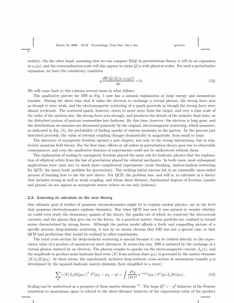
scale(s). On the other hand, assuming that we can compute Π(Q) in perturbation theory it will be an expansion
in αs(µ), and the renormalization scale will also appear in ratios Q/µ with physical scales. For such a perturbative
expansion, we have the consistency condition
µdΠ(Q, Q/µ, αs(µ))
dµ= 0 . (12)
We will come back to this relation several times in what follows.
The qualitative picture for DIS in Fig. 1 now has a natural explanation at large energy and momentum
transfer. During the short time that it takes the electron to exchange a virtual photon, the strong force acts
as though it were weak, and the electromagnetic scattering of a quark proceeds as though the strong force were
almost irrelevant. The scattered quark, however, starts to move away from the target, and over a time scale of
the order of the nucleon size, the strong force acts strongly, and produces the details of the inelastic final state, as
the disturbed system of partons reassembles into hadrons. By this time, however, the electron is long gone, and
the distributions we measure are detemined primarily by the original, electromagnetic scattering, which measures,
as indicated in Eq. (5), the probability of finding quarks of various momenta in the parton. As the process just
described proceeds, the value of relevant coupling changes dramatically in magnitude, from small to large.
The discovery of asymptotic freedom opened a new chapter, not only in the strong interactions, but in rela-
tivistic quantum field theory. For the first time, effects at all orders in perturbation theory gave rise to observable
consequences, and even the qualitative features of experiments could not be understood without them.
The explanation of scaling by asymptotic freedom played the same role for hadronic physics that the explana-
tion of elliptical orbits from the law of gravitation played for celestial mechanics. In both cases, most subsequent
applications were (and are) to much more complicated experiments (scale breaking, hadron-hadron scattering
for QCD, the many-body problem for gravitation). The striking initial success led to an essentially open-ended
process of learning how to use the new theory. For QCD, the problem was, and still is, to calculate in a theory
that includes strong as well as weak coupling, and whose short distance, fundmental degrees of freedom (quarks
and gluons) do not appear as asymptotic states (where we see only hadrons).
2.3. Learning to calculate in the new theory
One ultimate goal of studies of quantum chromodynamics might be to explain nuclear physics, say at the level
that quantum electrodynamics explains chemistry. But when QCD was new it was natural to wonder whether
we could even study the elementary quanta of the theory, the quarks out of which we construct the electroweak
currents, and the gluons that give rise to the forces. As a practical matter, these particles are confined in bound
states characterized by strong forces. Although the parton model affords a lively and compelling picture of a
specific process, deep-inelastic scattering, it was by no means obvious that DIS was not a special case, or that
QCD had predictions that would be realized in other experiments.
The total cross section for deep-inelastic scattering is special because it can be related directly to the expec-
tation value of a product of operators at short distances. It works this way. DIS is initiated by the exchange of a
virtual photon emitted by an electron. The photon couples to quarks via the electromagnetic current, Jµ(x), and
the amplitude to produce some hadronic final state |X〉 from nucleon state |pN 〉 is governed by the matrix elements
〈X |Jµ(0)|pN 〉. In these terms, the unpolarized, inclusive deep-inelastic cross section at momentum transfer q is
determined by the squared hadronic matrix elements (here simplified to a trace)
∑
X
| 〈X |Jµ(0)|pN 〉 |2 δ4(pX − pN − q) =
∫
d4y
(2π)4e−iq·y〈pN | Jµ(y)Jµ(0) |pN 〉 . (13)
Scaling can be understood as a property of these matrix elements 15. The large Q2 = −q2 behavior of the Fourier
transform to momentum space is related to the short-distance behavior of the expectation value of the product
March 10, 2006 10:58 Proceedings Trim Size: 9in x 6in qcd˙jets
7
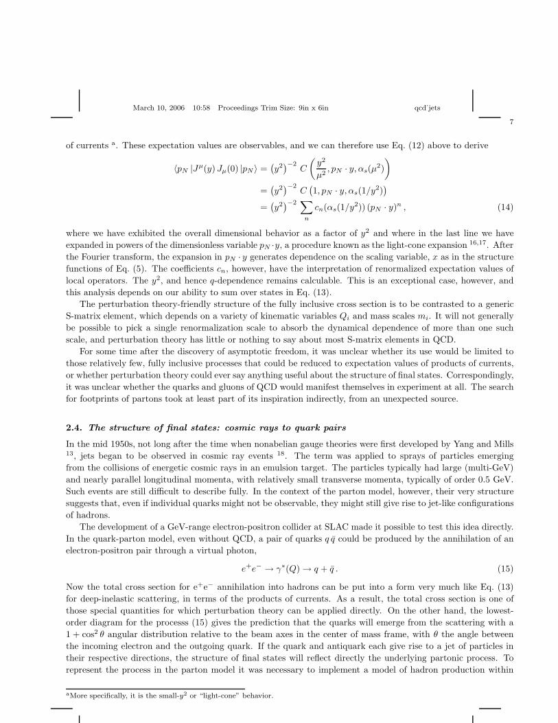
of currents a. These expectation values are observables, and we can therefore use Eq. (12) above to derive
〈pN |Jµ(y)Jµ(0) |pN 〉 =(
y2)−2
C
(
y2
µ2, pN · y, αs(µ
2)
)
=(
y2)−2
C(
1, pN · y, αs(1/y2))
=(
y2)−2 ∑
n
cn(αs(1/y2)) (pN · y)n , (14)
where we have exhibited the overall dimensional behavior as a factor of y2 and where in the last line we have
expanded in powers of the dimensionless variable pN ·y, a procedure known as the light-cone expansion 16,17. After
the Fourier transform, the expansion in pN · y generates dependence on the scaling variable, x as in the structure
functions of Eq. (5). The coefficients cn, however, have the interpretation of renormalized expectation values of
local operators. The y2, and hence q-dependence remains calculable. This is an exceptional case, however, and
this analysis depends on our ability to sum over states in Eq. (13).
The perturbation theory-friendly structure of the fully inclusive cross section is to be contrasted to a generic
S-matrix element, which depends on a variety of kinematic variables Qi and mass scales mi. It will not generally
be possible to pick a single renormalization scale to absorb the dynamical dependence of more than one such
scale, and perturbation theory has little or nothing to say about most S-matrix elements in QCD.
For some time after the discovery of asymptotic freedom, it was unclear whether its use would be limited to
those relatively few, fully inclusive processes that could be reduced to expectation values of products of currents,
or whether perturbation theory could ever say anything useful about the structure of final states. Correspondingly,
it was unclear whether the quarks and gluons of QCD would manifest themselves in experiment at all. The search
for footprints of partons took at least part of its inspiration indirectly, from an unexpected source.
2.4. The structure of final states: cosmic rays to quark pairs
In the mid 1950s, not long after the time when nonabelian gauge theories were first developed by Yang and Mills13, jets began to be observed in cosmic ray events 18. The term was applied to sprays of particles emerging
from the collisions of energetic cosmic rays in an emulsion target. The particles typically had large (multi-GeV)
and nearly parallel longitudinal momenta, with relatively small transverse momenta, typically of order 0.5 GeV.
Such events are still difficult to describe fully. In the context of the parton model, however, their very structure
suggests that, even if individual quarks might not be observable, they might still give rise to jet-like configurations
of hadrons.
The development of a GeV-range electron-positron collider at SLAC made it possible to test this idea directly.
In the quark-parton model, even without QCD, a pair of quarks q q could be produced by the annihilation of an
electron-positron pair through a virtual photon,
e+e− → γ∗(Q) → q + q . (15)
Now the total cross section for e+e− annihilation into hadrons can be put into a form very much like Eq. (13)
for deep-inelastic scattering, in terms of the products of currents. As a result, the total cross section is one of
those special quantities for which perturbation theory can be applied directly. On the other hand, the lowest-
order diagram for the processs (15) gives the prediction that the quarks will emerge from the scattering with a
1 + cos2 θ angular distribution relative to the beam axes in the center of mass frame, with θ the angle between
the incoming electron and the outgoing quark. If the quark and antiquark each give rise to a jet of particles in
their respective directions, the structure of final states will reflect directly the underlying partonic process. To
represent the process in the parton model it was necessary to implement a model of hadron production within
aMore specifically, it is the small-y2 or “light-cone” behavior.

March 10, 2006 10:58 Proceedings Trim Size: 9in x 6in qcd˙jets
8
the jet that included a cutoff in transverse momentum 19. The picture of the transition from partons to hadrons
is represented by Fig. 3.
θ?
θ
Figure 3. The parton to hadron transition for two jet events.
Would this picture be realized? It was, once the center of mass energy reached about 7 GeV 20, although to
see it at these energies took some analysis. Energies have increased a hundred-fold in the intervening time, and
jets have become a commonplace in high energy physics, in the final states of e+e− annnihilation, of deep-inelastic
scattering, and of hadron-hadron scattering, as illustrated by the next three figures. In deep-inelastic scattering,
for example, Fig. 4, the so-called “current jet” associated with the scattered quark is clearly visible. Fig. 5 shows
how well-defined two-jet events can be in electron-positron annihilation at energies around one hundred GeV, and
Fig. 6 shows a nice example of jets from proton-antiproton scattering in the TeV energy range.
Q**2 = 21475 y = 0.55 M = 198
Figure 4. A current jet in DIS. From the H1 Collaboration.

March 10, 2006 10:58 Proceedings Trim Size: 9in x 6in qcd˙jets
9
Y
XZ
200. cm.
Cent re of screen i s ( 0.0000, 0.0000, 0.0000)
50 GeV20105
Run:event 4093: 1000 Date 930527 Time 20716
Ebeam45.658 Evis 99.9 Emiss -8.6 Vtx ( -0.07, 0.06, -0.80)
Bz=4.350 Thrust=0.9873 Aplan=0.0017 Oblat=0.0248 Spher=0.0073
Ct rk(N= 39 Sump= 73.3) Ecal (N= 25 SumE= 32.6) Hcal (N=22 SumE= 22.6)
Muon(N= 0) Sec Vtx(N= 3) Fdet (N= 0 SumE= 0.0)
Figure 5. Two jet event in e+e− annihilation. From the OPAL Collaboration.
eta
-4.7 -3
-2 -1
0 1
2 3
4.7
phi180
0
360
ET(GeV)
385
Bins: 481Mean: 2.32Rms: 23.9Min: 0.00933Max: 384
mE_t: 72.1phi_t: 223 deg
Run 178796 Event 67972991 Fri Feb 27 08:34:03 2004
Figure 6. A “lego plot” representation of dijets in proton-antiproton scattering, represented in the space of rapidity and azimuthalangle with respect to the beam axis. From the D0 Collaboration.
2.5. Jets in QCD
By the time jets were first observed, asymptotic freedom had been discovered, and the basics of the analysis of
DIS, which we will review below, had been developed. The parton model had predicted the angular distributions
for jets that are initiated by electroweak processes such as e+e− annihilation and deep-inelastic scattering, but

March 10, 2006 10:58 Proceedings Trim Size: 9in x 6in qcd˙jets
10
gave little guidance on what those jets would actually look like, although it was thought that, as in cosmic ray
events, transverse momenta might be limited on the scale of some fraction of a GeV. At first, it was unclear
what QCD would have to say on this matter, until it was realized that perturbative field theory can make well-
defined predictions for certain observable quantities even though they cannot be written in terms of correlation
functions at short distances. These observables are not fully inclusive in the hadronic final state, but they do
sum over many final states. They are called “infrared safe” 21,22. Suitably-defined jet cross sections are part of
this class. To motivate infrared safety in QCD, we briefly recall the treatment of infrared divergences in quantum
electrodynamics.
In QED, infrared divergences are a direct result of the photon’s zero mass. One-loop corrections to QED
processes are typically finite if the photon is given a small mass λ, but diverge logarithmically as λ is taken to
zero, through terms like
∆σ(1)A→B (Q, me, mγ = λ, αEM) ∼ αEM σ
(0)A→B(Q, me)βAB(Q/me) ln
λ
Q. (16)
In this expression, σ(0)A→B is a lowest order cross section, characterized by momentum transfer Q and βAB is a
function that is independent of λ. The well-known solution of this problem 23 is to introduce an energy resolution,
∆E Q, and to calculate cross sections that sum over the emission of all soft photons with energies up to ∆E.
This is a realistic procedure, since any measuring apparatus has a minimum energy sensitivity, below which soft
photons will be missed in any case. The outcome of this procedure is that corrections to cross sections including
an energy resolution take the form,
∆σAB (Q, me, ∆E, αEM) ∼ αEM σ(0)A→B(Q, me)βAB(Q/me) ln
∆E
Q. (17)
The logarithm of the photon mass has been replaced by a logarithm of the energy resolution. Notice that if the
ratio ∆E/Q is not very very small, and if the function βAB is not very large, αEM ∼ 1/137 ensures that (17)
is numerically small. This explains the success of many lowest-order calculations in QED, in the face of that
theory’s infrared divergences.
The Bloch-Nordseick procedure in QED suggests that something similar might be possible in QCD. In this
case, however, since we want to use perturbation theory at high energy, we must be able to calculate in the limit
where the ratios of light quark masses to the energy scale become vanishingly small, along with those involving the
gluon mass, which is zero to start with. This leads to a whole new set of divergences, called collinear divergences,
which we will have occasion to discuss at length below. Something similar happens if we take the electron mass
to zero in Eq. (17), in which case the functions βAB develop logarithmic singularities.
Neglecting for the moment heavy quarks, we are after a set of cross sections that are perturbatively finite even
when all masses in the theory are set to zero. To go to high energy in perturbation theory, we must thus check
that we can go to the zero-mass limit. Once we can identify a quantity with a finite zero-mass limit, and have
traded zero mass back for high energy, we have a situation that is perfect for QCD. We will be able to use (12) to
pick the coupling at the scale of the energy, and asymptotic freedom will ensure that as the energy scale grows,
the relevant coupling will decrease. Perturbative predictions will then improve with increasing energy.
The classic analyses of Kinoshita and of Lee and Nauenberg 24 showed that total transition rates remain finite
in fully massless theories because the zero-mass limit does not violate unitarity in perturbation theory. Infrared
safe cross sections are generalizations of this analysis to less inclusive observables. For QED, this can be done
with an energy resolution; for QCD in the zero-mass limit, this is not sufficient. For e+e− annihilation, however,
we can identify infrared safe quantities by introducing an additional resolution. The motivation is completely
analogous to the QED case. In the limit of zero quark mass, a quark of momentum p, p2 = 0 can emit an gluon of
momentum xp, 0 < x < 1, (xp)2 = 0 and remain on-shell, since the remaining momentum (1−x)p is still lightlike
with positive energy. The resulting quark and gluon, however, are exactly collinear in direction, and it is by no

March 10, 2006 10:58 Proceedings Trim Size: 9in x 6in qcd˙jets
11
means clear how to resolve them, especially since the emission, or its inverse, can take place at any time, even
within a hypothetical detector. The same would be true for a massless electron and collinear photon.
If we draw an analogy to the energy resolution of QED, we are naturally led to seek observables with angular
as well as energy resolutions for high energy QCD (or massless QED), as represented in Fig. 7, where the cones
show an angular range into which large energy flows, while the small ball in the remaining directions represents
an energy resolution. Without going into detail yet, such cross sections are infrared safe, and depend only on
δ
εQ
Figure 7. Cone jets for e+e− annihilation.
the overall energy Q, the angular resolution δ, and the energy resolution εQ, with ε a small but finite number.
Because they are physical quantities, the perturbative expansions for the corresponding cross sections satisfy Eq.
(12), and we can write
σjet (Q/µ, δ, ε, αs(µ)) = σjet (1, δ, ε, αs(Q))
=∑
n≥0
Σn(δ, ε)αns (Q) . (18)
We can thus calculate these cross sections directly in perturbation theory 21, without needing to impose cutoffs
in transverse momentum. Infrared safety alone is sufficient to produce jet structure at high energies, since each
emission outside the cone is suppressed by a factor of αs(Q). The two-jet cross sections of e+e− of Fig. 7 can be
generalized in a number of ways that we will discuss below.
We may formalize the concept of infrared safety in the following way. QCD perturbation theory gives self-
consistent predictions for a quantity C when C:
• is dominated by short-distance dynamics in the infrared-regulated theory;
• remains finite when the regulation is taken away.
We will review in a little while how dimensional regularization can be used to control infrared, as well as ultraviolet,
divergences.
In “practical” terms, any perturbative cross section depends on all the mass scales (collectively, m) of the
theory in addition to the relevant kinematic variables (collectively, Q) C(m/µ, Q/µ, αs(µ)). An infrared safe
quantity is one whose perturbative expansion gives finite coefficients in the limit of zero fixed masses, m, up to
power corrections in m/Q,
C(m/µ, Q/µ, αs(µ)) =∑
n≥0
cn(0, Q/µ)αns (µ) + O
[(
m
Q
)p]
. (19)

March 10, 2006 10:58 Proceedings Trim Size: 9in x 6in qcd˙jets
12
with p > 0, typically an integer. Depending on the energy range and the quantity in question, the mass of a
heavy quark, one well above the QCD scale, may be treated as an m or as a Q.
3. Introduction to IR Analysis to All Orders
To explore further the theoretical basis of perturbative analysis we will work toward the proof of infrared safety for
certain cross sections, including those for jets in e+e− annihilation. Besides providing results that are interesting in
their own right, this will also provide methods for the analysis of electron-nucleon and nucleon-nucleon scattering,
as well as for processes involving heavy quarks.
To be specific, we will develop the following necessary ingredients, sketching, wherever space allows, arguments
that are applicable to all orders in perturbation theory.
• A review of the treatment of UV and IR divergences in dimensional regularization;
• A method to identify infrared sensitivity in perturbation theory: “physical pictures”;
• A method to identify IR finiteness/divergence: “infrared power counting”;
• An analysis of cancellation in cross sections: “generalized unitarity”.
The purpose of these discussions will be to explain the basis of, not to perform, explicit calculations.
3.1. UV and IR divergences in dimensional regularization
3.1.1. Navigating the n-plane
We will review a low order example of the use of dimensional regularization in due course, but even before that
we should clarify how this technique can be used to treat both the ultraviolet and infrared sectors of QCD.
The list below outlines in short the logical path from the Lagrangian of QCD to physically observable quantities
using dimensional regularization. It also helps to explain why infrared safety is essential in the comparison of
perturbative calculations to experiment.
LQCD → G(reg)(p1, . . . pn) , Re(n) < 4
→ G(ren)(p1, . . . pn) , Re(n) < 4 + ∆
→ S(unphys)(p1, . . . pn) , 4 < Re(n) < 4 + ∆
→ τ (unphys)(pi) , 4 < Re(n) < 4 + ∆
→ τ (phys)(pi) , n = 4 . (20)
First, by means of path integrals or the interaction picture, the Lagrangian LQCD generates a set of rules for
perturbation theory, out of which we may construct the Fourier transforms of time-ordered products of fields, the
Green functions, G(reg)(pi) as perturbative integrals over loop momenta. At this stage, we regularize the theory
by evaluating the loop integrals in a reduced number of dimensions, n < 4, and by keeping all momenta away from
particle poles (p2i 6= m2). If we do this (keeping away from points where subsums of momenta vanish), the only
poles in the n plane are ultraviolet poles. These off-shell, regularized Green functions are defined only for n < 4.
In these terms, renormalization is a systematic procedure for removing all singularities at n = 4 in regularized
Green functions. The resulting renormalized Green functions, G(ren)(pi) may then be analytically continued to
any n whose real part is less than or equal to 4 + ∆, for some ∆ > 0.
For an infrared finite theory, this would be enough, and we could safely set n = 4, and start evaluating S-matrix
elements and other physical quantities. For QCD, however, our job is not done yet, because at n = 4 the Green
functions encounter a host of infrared, including collinear, singularities. As a result, its perturbative S-matrix
elements are hopelessly ill-defined. Our next step is rather to continue into the window 4 < Re(n) < 4+∆. In this
range, we are still to the left of the ultraviolet divergences of the renormalized theory, and (as we shall see below)

March 10, 2006 10:58 Proceedings Trim Size: 9in x 6in qcd˙jets
13
to the right of infrared divergences, which appear in dimensional regularization as poles with Re(n) ≤ 4. In this
infrared-regulated range we can actually take the limits p2i → m2
i and construct the S-matrix, for all quarks and
even for the massless gluon.
The S-matrix elements computed for Re(n) > 4 are not physical of course, because they have been computed
in QCD in more than four dimensions. They are not even “close” to the physical quantities of QCD, as is manifest
by their ubiquitous 1/(n − 4) poles. By contrast, however, if we can systematically construct quantities τ(n),
which are at the same time observable and free of poles at n = 4, the τ ’s can be returned smoothly to the physical
theory. The criterion that they lack infrared poles may be taken as an indication that they are dominated by the
short-distance behavior of the theory. These are the quantities to which asymptotic freedom can be applied to
provide infrared safe predictions that we may compare to experiment. Let us see how these ideas are realized for
the simplest of cases, the total cross section for e+e− annihilation to hadrons.
3.1.2. The total annihilation cross section
The process e+e− → hadrons already proceeds at zeroth order in αs through annihilation to quarks, via the
photon and the Z: e+e− → quark + antiquark, as in Fig. 8. Specializing for the moment to a virtual photon, we
Q2
q
q_
2e
e +
-
γZ ,
Figure 8. Lowest order e+e− annihilation to quarks.
can readily derive from Fig. 8 the total cross section for unpolarized annihilation at center of mass energy Q,
σ(0)total = Ncolors
4πα2EW
3Q2
∑
f
Q2f , (21)
which is, in fact, a pretty good approximation to the total cross section below the Z pole, if we count in the sum
over flavors those quark pairs that can be produced at a given energy. In this way, Eq. (21) is a nice test of quark
masses and charges, Q2f = 4/9, 1/9, and Ncolors = 3. From our previous discussions, we expect this lowest-order
perturbative prediction to make sense for the same reason that lowest-order perturbative cross sections make
sense in QED. The cross section σtotal is infrared safe, and as a result, corrections will appear as a power series
in αs(Q), which is relatively small once the total energy is well into the GeV range. Let’s see how this works at
first order in αs.
Diagrams relevant the order-αs corrections to the zeroth-order cross section are shown in Fig. 9. The first
QCD correction (next-to-leading order, or NLO) is
σ(1)total = σ
(1,qqg)total + σ
(1,qq)total , (22)
the sum of contributions from both three-particle (quark-antiquark-gluon) and two-particle (quark-antiquark)
final states.
Consider first the three-particle final state. Its contribution to the cross section is proportional to the lowest
order cross section (21),
σ(1,qqg)total = σ
(0)total
(αs
π
)
(
CF
π
)
I3(Q) , (23)

March 10, 2006 10:58 Proceedings Trim Size: 9in x 6in qcd˙jets
14
+ 2
Figure 9. Diagrams for the order αs correction to the annihilation cross section.
where CF = (N2c − 1)/2Nc = 4/3 for QCD, and I3(Q) is proportional to the integral over three-particle phase
space of the squared amplitude for gluon emission (here in four dimensions),
I3(Q) = (2π)
∫ Q/2
0
dk k
∫ π
0
dθ sin θ
[
(Q − 2k)
(Q − k(1 − u))2
]
×[
[Q − (1 − u)k]2
k2(1 − u2)+
Q(1 + u)
(Q − 2k)(1 − u)
]
. (24)
Here k is the gluon energy, θ = θp1k is the angle between the quark and gluon momenta, and u ≡ cos θ. In this
form, collinear divergences are manifest at u → ±1, and infrared (soft gluon) divergences at k → 0. Notice that
in this case there is no collinear divergence at k = Q, which corresponds to the quark and antiquark becoming
parallel, or at zero momentum for the quark or antiquark.
To exhibit the leading divergences, we simplify (24) to an approximation relevant to small k and θ:
I3,IR = (2π)
∫
0
dk
k
∫
0
dθ
θ. (25)
We now briefly review how dimensional regularization takes care of the singularities of these integrals.
3.1.3. Infrared dimensional regularization in a nutshell
We can develop the essentials of dimensional regularization as applied to infrared divergences by the following
steps,
I3,IR = (2π)
∫
0
dk
k
∫
0
dθ
θ
∼∫
0
dk
k2
∫
0
dθ
θ2
[
(k sin θ)
∫ 2φ
0
dφ
]
=
∫
0
dk
k2
∫
0
dθ
θ2[(k sin θ)mΩm]m=1 (26)
where in the second line we reexpressed the factor 2π as the integral over the azimuthal angle. To motivate
the third expression we simply observe that the azimuthal angular integral is just a special case Ω1 of Ωm, the

March 10, 2006 10:58 Proceedings Trim Size: 9in x 6in qcd˙jets
15
angular integration in polar coordinates for m + 1 dimensions, and that the volume element in m + 2 dimensions
is precisely (k sin θ)mΩm, for m any integer b
With this in mind, we reinterpret the parameter m in Eq. (26), which in the unregularized theory has the value
unity, as a complex parameter, and redefine Ωm as a complex function Ω(m) of m, restricted to be the angular
volume Ωm in m + 1 dimensions for any integer value of m. This turns out to be enough to define Ω(m) uniquely
for all complex m,
Ωd =2π(d+1)/2
Γ(
12 (d + 1)
)
= 2dπd/2 Γ(
12d)
Γ(d), (27)
with Γ(z) the Euler Gamma function, with the well-known properties,
Γ(1/2) =√
π,
zΓ(z) = Γ(z + 1),
Γ(N) = (N − 1)! , (28)
where N is an integer. With these properties we easily check the angular volumes for low dimensions: m + 1 =
2 (2π), 3 (4π), 4 (2π2).
For Re(m) > 1, I3,IR becomes finite, and the soft and collinear divergences appear as poles at m = 1, as
anticipated,
I3,IR ∼ Ωm
∫
0
dk
kkm−1
∫
0
dθ
θθm−1 ∼ 1
(1 − m)2. (29)
This proceedure defines a new theory: QCD in 4 + (m − 1) dimensions, where m = 1 is real QCD.
A similar continuation in dimension can always be found for any observable, since whenever we continue
expressions to n > 4, we will be able to integrate over the angular phase space for dimensions above n = 4.
This, in turn, will regulate the remaining integrals. Analogous considerations apply to the ultraviolet divergences
regulated with n < 4 as in Eq. (20) above 25.
Our notation below will generally be to take n as the number of dimensions, and to express variations away
from n = 4 through ε = 2−n/2. Again, we emphasize that it is only infrared safe quantities that can be evaluated
at ε = 0, where they return to the “real” theory.
For the case at hand, in n = 4 − 2ε-dimensional QCD, we found double and single poles in I3,IR. The full
expression is also straightforward to evaluate, up to terms that vanish for ε → 0, and σ(1,qqg)total is given in this
approximation by
σ(1,qqg)total (Q, ε) = σ
(0)total CF
(αs
π
)
[
1
ε2+
3
2ε− π2
2+
19
4
]
. (30)
Clearly, the three-particle contribution to the total cross section is highly singular when returned to four dimen-
sions. Although unphysical, it is positive, corresponding to the absolute square of the amplitude for the emission
of a single gluon.
Dimensional regularization, however, also enables us to compute the two-particle contribution, given by one-
loop vertex and self-energy diagrams. This calculation is perhaps more familiar, since it can be carried out in
terms n-dimensional loop integrals. Unlike the three-particle cross section, it is not an absolute value squared,
bThis is easy to verify inductively, using polar coordinates in N dimensions to define cylindrical coordinates in N + 1 dimensions asan intermediate step.

March 10, 2006 10:58 Proceedings Trim Size: 9in x 6in qcd˙jets
16
and need not be positive. The result is proportional to the lowest order cross section, and is given by
σ(1,qq)total (Q, ε) = −σ
(0)total CF
(αs
π
)
[
1
ε2+
3
2ε− π2
2+ 4
]
. (31)
Here we see the same poles as in the three-particle case, but now with negative rather than positive signs. As
expected the sum of the two- and three-particle NLO cross sections is finite, and the total NLO cross section is
very simple,
σ(1)total(Q, ε) = σ
(0)total CF
(αs
π
)
[
3
4
]
, (32)
a satisfying result that is nonsingular ε, and can hence be returned smoothly to four dimensions.
Our goal is now to identify classes of cross sections, involving jets and related observables, for which we know
ahead of time that calculations like these will provide predictions at ε = 0, that is, for real QCD. To do so, we
need first to develop a better understanding of where poles in ε come from, not only at NLO, but to all orders in
the coupling.
3.2. Physical pictures
Divergences in perturbation theory can come about in only two ways: either from the infinite volume of momentum
space, or from infinities in the integrands of individual diagrams. In renormalized perturbation theory, the former
are eliminated by the systematic construction of counterterms. The latter, of course, reflect the vanishing of the
causal propagators: k2−m2 + iε = 0, where m may or may not be zero. We have kept the infinitesimal imaginary
part of the propagator to remind ourselves that perturbation theory is defined by integrals in the complex plane
of every loop momentum component. The integrand of any diagram is thus a meromorphic function of the 4L
complex variables of integration in four dimensions, where L is the number of independent loop momenta. This
will be a very useful observation, as we shall soon see.
To begin with a specific example, consider the one-loop quark electromagnetic form factor, the sum of the
lowest-order vertex and self-energy corrections to the electromagnetic current,
Γµ(q2, ε) = −eµε u (p1)γµv(p2) ρ(q2, ε) . (33)
The function ρ(q2, ε) is the correction that appears times the lowest order annihilation cross section, Eq. (31) at
NLO for the two-particle final state,
ρ(q2, ε) = −αs
2πCF
(
4πµ2
−q2 − iε
)εΓ2(1 − ε)Γ(1 + ε)
Γ(1 − 2ε)
1
(−ε)2− 3
2(−ε)+ 4
. (34)
Because the electromagnetic current is conserved, the ultraviolet divergences in the sum of diagrams cancel, and
no counterterms are necessary in this computation.
The infrared poles of dimensional regularization, which diverge at n = 4, require, as pointed out above, that
some lines go on-shell lines for some real values of the loop momenta. But on-shell lines at real momenta are not
enough. The momentum integrations, interpreted as contours in complex planes must also be pinched between
coalescing poles, at least one pole on either side of the contour. If not, Cauchy’s theorem can be used to deform
the contour(s) away from the poles so that the integral can carried out in such a way that the integrand is always
finite. The requirement that the contours be pinched makes it possible to identify potential sources of infrared
singularities systematically.
Consider a particular subspace of the momentum space of a given diagram where some set of propagators
diverge, that is, where some set of lines are on-shell. We’ll refer to such a subspace as a “singular surface” of
loop momentum space. Let us contract all the lines that are not on-shell at the singular surface to a point. The
resulting diagram is called a reduced diagram. The singular surface can give rise to a divergence only if all the
loop momenta of the reduced diagram are pinched between coalescing singularities at the surface. We therefore

March 10, 2006 10:58 Proceedings Trim Size: 9in x 6in qcd˙jets
17
refer to such a surface as a “pinch surface”. The existence of a pinch surface is a necessary condition for the
production of an infrared pole.
It is natural to think of the reduced diagram, all of whose lines are on shell as the picture of a process, but
in fact this is not automatic. In a physical process, particles travel between points, represented by the vertices
where they begin and end. In these terms, we can use a criterion identified by Coleman and Norton 26,27 and
distinguish pinch surfaces solely on the basis of their reduced diagrams: the lines of the reduced diagram must
describe a scattering process in which classical point particles move between vertices, such that all their motions
are mutually consistent.
To be specific, for a reduced diagram with lines of momenta pk to correspond to a pinch surface, we must be
able to assign to each of its vertices i a position xi in space-time such that if vertices i and j are connected by
line k, with x0i > x0
j , then
(xi − xj)µ = (x0
i − x0j ) vµ
k , (35)
where vk = pk/p0k is the four-velocity associated with the on-shell momentum pk. This corresponds to free
propagation between vertices in space-time. The condition (35) is invariant under a scale transformations for all
points, keeping momenta fixed: xi → λxi, for all i. For arbitrary λ > 1, the process simply “gets larger”, and we
can think of this as a potential source of the infrared divergences.
The proof of this assertion is easy, and may be demonstrated adequately by a simple example, the triangle
diagram in Fig. 9. Because the divergences are associated with momentum dependence in denominators, we
simplify further by suppressing all numerator factors, and just study the scalar triangle diagram with light-like
external momenta, p1 and p2,
I∆(p1, p2) =
∫
dnk
(2π)n
1
(k2 + iε) ((p1 − k)2 + iε) ((p2 + k)2 + iε), (36)
which, introducing Feynman parameters, can be expressed in terms of a single denominator, D, that is quadratic
in the momenta,
I∆(p1, p2) = 2
∫
dnk
(2π)n
∫ 1
0
dα1dα2dα3 δ(1 −∑3i=1 αi)
D3
D = α1k2 + α2(p1 − k)2 + α3(p2 + k)2 + iε . (37)
Because D is quadratic, its zeros, and therefore the points at which the integrand diverges, are simply the solutions
to a quadratic equation in each momentum component. A necessary condition that each momentum component
be pinched between singularities is that the two solutions for each kµ must coincide, µ = 0 . . . 3, so that
∂
∂kµD(αi, k
µ, pa) = 0 . (38)
For the case at hand this leads to the following conditions,
α1k − α2(p1 − k) + α3(p2 + k) = 0
m∆t1vk − ∆t2vp1−k + ∆t3vp2+k = 0 , (39)
in terms of times given by ∆ti = αi p0i and velocities pi/p0
i , as noted above. The second condition is the statement
that if we start at any one of the three vertices, the total four-distance travelled by going around the loop is
zero. This is equivalent to the statement that the points are connected by classical propagation for each of the
three particles. Now in fact, for specific solutions, one or two of the times may vanish. Indeed, whenever a line is
off-shell, its corresponding α parameter must vanish, or we may deform the α contour and avoid the point D = 0
without worrying at all about the momenta. The points αi = 0, however, are boundaries of the α integrals. These
boundaries define the integrals, and therefore cannot be avoided by contour deformation. The vanishing of an

March 10, 2006 10:58 Proceedings Trim Size: 9in x 6in qcd˙jets
18
αi normally corresponds to the vanishing of the time of propagation for an off-shell particle, one contracted to a
point in the corresponding reduced diagram.
There are three solutions for Eq. (38), which illustrate the generic physical interpretations of e+e− annihilation
processes.
• Collinear to p1: in which two particles of momentum p1− k and k are on-shell and exactly parallel to one
of the external lines. The third line, with momentum (p2 + k) is off-shell, and its time of propagation is
correspondingly zero
k = ζp1 , α3 = 0 , α1ζ = α2(1 − ζ) . (40)
• Collinear to p2:
k = −ζ′p2 , α2 = 0 , α1ζ′ = α3(1 − ζ′) . (41)
• Soft: for which the solution is α1 = 1, while the velocity of the zero-momentum particle is undefined.
There are similar pinch surfaces when the remaining two momenta vanish. The physical picture in this
case may be thought of as an infinite-wavelength soft particle coupling to finite momentum particles at
arbitrary points in space-time,
kµ = 0 , (α2/α1) = (α3/α1) = 0 . (42)
These configurations show that the sources of infrared sensitivity that we identified above for the high-energy
and/or zero mass limits, collinear and soft, correspond directly to pinch surfaces, at least for the example that
we have examined. The same analysis, however, can be carried out in just the same way for an arbitrary diagram
with arbitrary numbers of loops. This leads to the generalization of Eq. (38) known as the Landau equations 28,
for all i : `2i = m2
i , and/or αi = 0,
and∑
i in loop s
αi`iεis = 0 , (43)
where εis =1 (-1) for loop momentum i flowing along (opposite to) momentum `i, and 0 otherwise. Generalizing
Eq. (39), the consistency of the physical picture associated with an arbitrary pinch surface is ensured by the
identity
∆x12 + ∆x23 + . . . + ∆xn1 = 0 (44)
around each loop of the diagram, of the sort in Fig. 10.
Figure 10. Loop illustrating the physical condition (44).
The interpretation of pinch surfaces, and hence of the possible sources of infrared poles, in terms of physical
pictures greatly simplifies the process of classifying their origin in many cases, particularly for processes involving
hard scatterings. As we have suggested above, however, satisfying the Landau equations is still only a necessary,
March 10, 2006 10:58 Proceedings Trim Size: 9in x 6in qcd˙jets
19
and not sufficient condition for an infrared divergence. Clearly, the strength of the singularity on the pinch
surface plays a role as well. This leads us to power counting, which provides us with a method for distinguishing
singularities that can give rise to divergences from those that cannot.
3.3. Power counting
As with our analysis of physical pictures, our goal in analyzing the strength of singularities by power counting
is to find necessary conditions for divergences. Until we do a specific integral in detail, it is always possible that
an unexpected symmetry or cancellation between diagrams might eliminate an apparent singularity. Indeed, in
gauge theories conspiracies between diagrams are more common that not, because only in gauge-invariant sums
do unphysical modes decouple from physical quantities. Without going into detail right here, it is worth pointing
out that unphysical modes often give rise to unphysical infrared poles in individual diagrams 29.
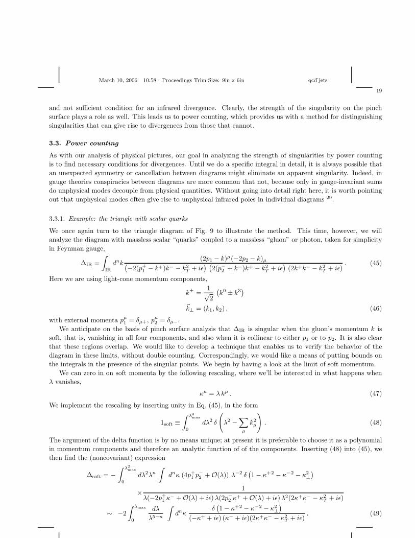
3.3.1. Example: the triangle with scalar quarks
We once again turn to the triangle diagram of Fig. 9 to illustrate the method. This time, however, we will
analyze the diagram with massless scalar “quarks” coupled to a massless “gluon” or photon, taken for simplicity
in Feynman gauge,
∆IR =
∫
IR
dnk(2p1 − k)µ(−2p2 − k)µ
(
−2(p+1 − k+)k− − k2
T + iε) (
2(p−2 + k−)k+ − k2T + iε
)
(2k+k− − k2T + iε)
. (45)
Here we are using light-cone momentum components,
k± =1√2
(
k0 ± k3)
~k⊥ = (k1, k2) , (46)
with external momenta pµ1 = δµ+, pµ
2 = δµ−.
We anticipate on the basis of pinch surface analysis that ∆IR is singular when the gluon’s momentum k is
soft, that is, vanishing in all four components, and also when it is collinear to either p1 or to p2. It is also clear
that these regions overlap. We would like to develop a technique that enables us to verify the behavior of the
diagram in these limits, without double counting. Correspondingly, we would like a means of putting bounds on
the integrals in the presence of the singular points. We begin by having a look at the limit of soft momentum.
We can zero in on soft momenta by the following rescaling, where we’ll be interested in what happens when
λ vanishes,
κµ = λkµ . (47)
We implement the rescaling by inserting unity in Eq. (45), in the form
1soft ≡∫ λ2
max
0
dλ2 δ
(
λ2 −∑
µ
k2µ
)
. (48)
The argument of the delta function is by no means unique; at present it is preferable to choose it as a polynomial
in momentum components and therefore an analytic function of of the components. Inserting (48) into (45), we
then find the (noncovariant) expression
∆soft = −∫ λ2
max
0
dλ2λn
∫
dnκ (4p+1 p−2 + O(λ)) λ−2 δ
(
1 − κ+2 − κ−2 − κ2⊥
)
× 1
λ(−2p+1 κ− + O(λ) + iε)λ(2p−2 κ+ + O(λ) + iε)λ2(2κ+κ− − κ2
T + iε)
∼ −2
∫ λmax
0
dλ
λ5−n
∫
dnκδ(
1 − κ+2 − κ−2 − κ2⊥
)
(−κ+ + iε) (κ− + iε)(2κ+κ− − κ2T + iε)
. (49)

March 10, 2006 10:58 Proceedings Trim Size: 9in x 6in qcd˙jets
20
We have dropped terms that are higher order in λ in both numerator and denominator. The integral is then
homogeneous in λ, and the λ integral can be performed to give a 1/ε pole in n dimensions. The remaining integral
is free of soft divergences since κ2 is fixed at unity. The soft divergence, where all components of momentum
vanish together, has therefore been isolated by the scaling (47). This does not mean that the remaining integral
is finite in four dimensions, however, and we easily verify additional singularities associated with the presence
of collinear divergences at finite kµ, and arbitrarily close to the point kµ = 0. These can be treated in much
the same fashion as for the original diagram, by using the delta function to do one of the κ integrals, and then
analyzing the analytic structure of the remaining integral.
The additional collinear divergences appear in the κ integrals as pinches at the surfaces defined by
κ± = 1 ,
κ∓ = κ2T = 0 , (50)
where we note that the variables κ are dimensionless. These are the soft tails of the collinear regions, and following
a similar analysis we find that they produce double poles. For example, for the pinch surface where κ+ = 1 we
may introduce a second scaling,
κ−′ = λ′ κ−, κ′T
2 = λ′ κ2T , λ′2 = κ−2 + (κ2
T )2 , (51)
and verify that the λ′ integral, which now controls the approach to the pinch surface, produces a seond pole in ε.
The remaining integrals are then manifestly finite. We discover in this way the double poles for the scalar quark
vertex; going through identical steps in QCD will give the same result. We now turn to a more general analysis.
3.3.2. General pinch surface analysis
As in the discussion of the Landau equations, the steps from the specific example to a general analysis are clear.
Suppose we consider an arbitrary graph G(Q) with specified external momenta, denoted collectively by Q. Using
the physical picture analysis, we can in principle identify every pinch surface γ of G(Q). At any point on γ, we
may divide the coordinates of the loop momentum space into “internal” coordinates, `b that specify directions
within the surface γ, and “normal” coordinates, κa that specify directions that move us off the surface. For
example, for the soft divergence of the triangle diagram the pinch surface is a point, so that for this surface all
corrdinates kµ are normal coordinates. For the collinear-p1 pinch surface, with p1 in the plus direction, the plus
component of the k loop momentum is internal, while the minus and transverse are normal.
Isolating the integral of G(Q) near γ the same way we treated the triangle diagram near the soft pinch surface
(point), we write in dimensional regularization
Gγ(Q) =
∫
γ
∏
b
d`b
∫
γ
Dγ(ε)∏
a=1
dκa
∏
i ni(κa, `b, Q)∏
j dj(κa, `b, Q), (52)
where the numerator factors ni and denominator factors dj are polynomials in the normal and intrinsic coordinates,
along with the external momenta. Any Jacobean factors are absorbed into the definitions of the volume elements,
and the parameter Dγ(ε) represents the number (possibly noninteger) of normal variables. Once again, we insert
unity in the form of a scaling for the normal coordinates (only), κa = λγ κ′a,
1γ =
∫ (λmaxγ )2
0
dλ2γ δ
(
λ2γ −
∑
a
κ2a
)
=
∫ (λmaxγ )2
0
dλ2γ
λ2γ
δ
(
1 −∑
a
κ′a2
)
. (53)
As above, the choice of normal coordinates will depend on the pinch surface.
March 10, 2006 10:58 Proceedings Trim Size: 9in x 6in qcd˙jets
21
Under the scaling, both numerators and denominators have dominant terms in the λ → 0 limit, the terms of
lowest overall powers Ni and Dj of normal coordinates, respectively,
ni(κa, `b, Q) = λNiγ [ni(κ
′a, `b, Q) + O(λ)]
dj(κa, `b, Q) = λDjγ
[
dj(κ′a, `b, Q) + O(λ)
]
. (54)
In terms of the exponents Ni and Dj , we find in this approximation an overall scaling behavior as we approach
the singular surface, given by
Gγ(Q) = 2
∫ λmaxγ
0
dλ
λpγ∆γ(Q)
pγ =∑
j
Dj + 1 −Dγ(ε) −∑
i
Ni . (55)
∆γ(Q) is the remaining integral, in which every numerator and denominator factor has been replaced by its term
of lowest homogeneity in the κ’s,
∆γ(Q) =
∫
O(Q)
∏
b
d`b
∫
γ
Dγ(ε)∏
a=1
dκ′a
∏
i ni(κ′a, `b, Q)
∏
j dj(κ′a, `b, Q)
δ
(
1 −∑
a
κ′a2
)
. (56)
On this basis, we estimate the contribution from the pinch surface γ in dimensional regularization as the result
of the λ integral, times whatever the remaining integral ∆γ(Q) gives.
In general, the integral ∆γ(Q) will have additional pinch surfaces, of course. If, however, these pinch surfaces
are among the original set of surfaces identified for the graph G(Q), we can bound the behavior of ∆γ(Q) on
this basis, and eventually bound the entire integral by an expression that has some maximal number of poles
(possibly none) in ε = 2− n/2. This situation is by no means assured, however, and different classes of diagrams
require different choices of normal coordinates. It is by this reasoning that we verify, however, the infrared safety
of classes of jet and related cross sections. These cross sections are in general not free of pinch surfaces, but are
defined in such a way that these pinch surfaces are not strong enough to produce poles in ε.
We note that this analysis is simpler for massless quarks. Organizing poles in dimensional regularization is
more complicted in the presence of quark masses, simply because the masses provide additional scales.
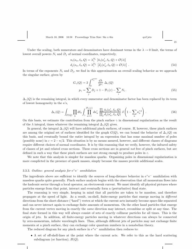
3.3.3. Outline: general analysis for e+e− annihilation
The ingredients above are sufficient to identify the sources of long-distance behavior in e+e− annihilation with
massless quarks quite generally. Pinch surface analysis begins with the observation that all momentum flows into
the hadronic sector through a local operator, an electroweak current. We must identify all physical pictures where
particles emerge from that point, interact and eventually form a (perturbative) final state.
The reasoning is very simple, keeping in mind that all particles are taken to be massless, and therefore
propagate at the speed of light. As a result, on-shell, finite-energy particles that emerge moving in different
directions from the short-distance (“hard”) vertex at which the current acts instantly become space-like separated
and can never interact again to exchange finite amounts of momentum. On the other hand particles that emerge
from the current vertex moving in exactly the same direction may interact, recombine or split at any time. The
final state formed in this way will always consist of sets of exactly collinear particles for all times. This is the
origin of jets. In addition, all finite-energy particles moving in whatever directions can always be connected
by zero-momentum, infinite wavelength lines. Thus, although different jets of particles may not exchange finite
momenta at a pinch surface, they can exchange color quantum numbers in a nonabelian theory.
The reduced diagram for any pinch surface in e+e− annihilation then reduces to:
• A set of off-shell-lines at the point where the current acts. We refer to this as the hard scattering
subdiagram (or function), H(Q).

March 10, 2006 10:58 Proceedings Trim Size: 9in x 6in qcd˙jets
22
• A set of jet subdiagrams, Ji of exactly collinear lines that emerge from the hard scattering through one or
more finite-energy “jet lines”, which rearrange themselves into any number of particles, all moving with
exactly parallel momenta.
• A soft subdiagram, S, made up of lines whose momenta vanish at the pinch surface. The soft subdiagram
may be connected to any of the jet subdiagrams, or to the hard subdiagram through zero-momentum
lines.
Power counting, carried out as above, may be extended to pinch surfaces of semi-inclusive cross sections, by
scaling final-state mass shell delta functions in the same way as propagators, which have the same dimensions
and homogeneity properties, δ+(k2) ↔ 1/k2. In this manner, we can show that in a gauge theory like QCD,
cross sections with fixed numbers of particles, but with the same dimension as the total cross section are at worst
logarithmically divergent, and have up to two poles in ε per loop 27. We will refer to such cross sections as
semi-inclusive. They are simply cross sections for which every particle in the final state is integrated over at least
part of its phase space.
Space does not allow a detailed proof of logarithmic power counting, but we can think about it in the following
way for the the quark-antiquark production process. We have already seen that the one-loop vertex diagram is
logarithmically divergent for n = 4. Now let’s consider what happens when we attach an extra gluon line to the
vertex diagram, so as to preserve the pinch surface structure.
Adding one additional vector line to such a diagram increases the number of lines by at most three, and
increases the number of loops by one. If the line is soft we may choose the normal variables as all four of the loop
momentum components. If we attach the soft line at each end to jet lines, the denominators of the new jet lines
are linear in the soft momentum, while the denominator of the new soft line is quadratic. Scaling the new soft
loop along with the original diagram we find an extra power λ−4 from the new denominators and λ4 from the
new loop momentum, so that the power counting remains unchanged. Adding a jet line leads to the same result,
once the scaling dependence of momentum factors in the numerator are taken into account.
For a process which like e+e− annihilation has a single hard scattering in its reduced diagram, we may choose
normal variables according to the example shown above. The reduced diagram for any such pinch surface will
be characterized by a set of jets, which we may label by index i. Fig. 11 shows a typical example of a reduced
diagram, with two jets for simplicity. The figure is presented as a cut diagram, with the perturbative contribution
to the amplitude on the left, and the complex conjugate amplitude on the right. The pinch surface analysis and
power counting described above is readily extended to cut diagrams through the power-counting correspondence
of mass-shell delta functions and propagators just noted.
The overall power of λµ(γ)−1 for pinch surface γ may be thought of as defining a “superficial” degree of infrared
divergence, µ(γ) (the extra -1 is compensated by the volume element dλ) . The precise graphical and momentum
flow configuration of the reduced diagram are directly reflected in the value of µ(γ). At an arbitrary pinch surface,
we may identify a number of relevant integer parameters, associated with the hard, jet and soft subdiagrams, that
provide a lower bound on the degree of infrared divergence.
• Some numbers H(L,R)i ≥ 1 of lines attach the jets in the amplitude and its complex conjugate (to the left
and right of the final-state “cut” in a cut diagram). In the Hs we count only quark lines and those gluon
lines with transverse polarizations at the pinch surface. (In covariant gauges, ghost lines should also be
counted.) The contributions from pinch surfaces where one or more jets connect to a hard scattering by
only unphysical gluon polarizations vanish 29 by the Ward identities of QCD, which ensure that physical
states evolve into physical states only.
• A(L,R)i unphysically polarized gluons may, however, appear as additional gluon lines attached to the hard
scatterings.
• The soft function S may attach to the jet subdiagram Ji, i = 1 . . . J in an arbitrary fashion, by the
exchange of soft gluons, and in the general case soft quarks and even ghosts in covariant gauges. We

March 10, 2006 10:58 Proceedings Trim Size: 9in x 6in qcd˙jets
23
Figure 11. Representative two-jet reduced diagrams for jet cross section in cut diagram notation: (a) physical gauge; (b) covariantgauge. From Ref. 30.
denote the number of soft gluons, quarks (antiquarks) and ghosts that connect S with Ji as ai, qi and ci,
respectively.
• Some numbers of soft lines S(L,R) may attach S to the left and right hard scattering vertices. (Such lines
are not shown in figure.)
The minimal superficial degree of infrared divergence for an arbitrary J-jet pinch surface in covariant gauges
may be computed in terms of these parameters and is given in four dimensions by 27
µ(γ) = S(L) + S(R) +1
2
J∑
jets i=1
H(L)i + H
(R)i − 2 + 2qi + ci +
[
A(L)i + A
(R)i + ai − u
(3)i
]
. (57)
where u(3)i is the number of three-point vertices in jet i to which soft gluons ai or jet gluons Ai connect. In
physical gauges, the terms involving the Ais are absent.
The minimal value of µ(γ) of a given cut diagram defines the most divergent, or “leading” pinch surfaces
(referred to as “leading regions” in Refs. 27,30). For negative µ(γ) we have an overall power divergence; for
µ(γ) = 0 the overall divergence is logarithmic, and for positive µ(γ) the pinch surface does not produce a
divergence at all.
For an arbitrary pinch surface relevant to a semi-inclusive cross section in e+e− annihilation, we easily verify
that the µ(γ) ≥ 0. The lower limit, corresponding to logarithmic divergence, is realized only for reduced diagrams
like the ones of Fig. 11. These are characterized by quite specific conditions on the variables above.
• At most a single quark or physically polarized gluon connects each hard scattering vertex to each jet:
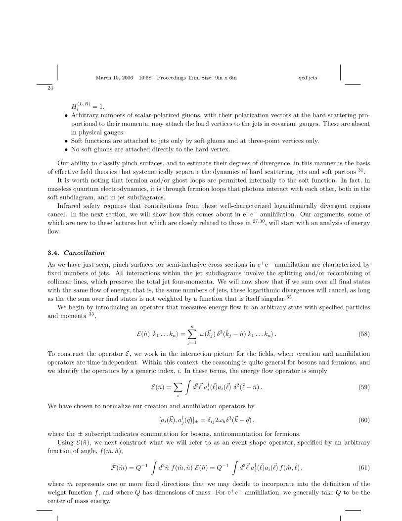
March 10, 2006 10:58 Proceedings Trim Size: 9in x 6in qcd˙jets
24
H(L,R)i = 1.
• Arbitrary numbers of scalar-polarized gluons, with their polarization vectors at the hard scattering pro-
portional to their momenta, may attach the hard vertices to the jets in covariant gauges. These are absent
in physical gauges.
• Soft functions are attached to jets only by soft gluons and at three-point vertices only.
• No soft gluons are attached directly to the hard vertex.
Our ability to classify pinch surfaces, and to estimate their degrees of divergence, in this manner is the basis
of effective field theories that systematically separate the dynamics of hard scattering, jets and soft partons 31.
It is worth noting that fermion and/or ghost loops are permitted internally to the soft function. In fact, in
massless quantum electrodynamics, it is through fermion loops that photons interact with each other, both in the
soft subdiagram, and in jet subdiagrams.
Infrared safety requires that contributions from these well-characterized logarithmically divergent regions
cancel. In the next section, we will show how this comes about in e+e− annihilation. Our arguments, some of
which are new to these lectures but which are closely related to those in 27,30, will start with an analysis of energy
flow.
3.4. Cancellation
As we have just seen, pinch surfaces for semi-inclusive cross sections in e+e− annihilation are characterized by
fixed numbers of jets. All interactions within the jet subdiagrams involve the splitting and/or recombining of
collinear lines, which preserve the total jet four-momenta. We will now show that if we sum over all final states
with the same flow of energy, that is, the same numbers of jets, these logarithmic divergences will cancel, as long
as the the sum over final states is not weighted by a function that is itself singular 32.
We begin by introducing an operator that measures energy flow in an arbitrary state with specified particles
and momenta 33,
E(n) |k1 . . . kn〉 =
n∑
j=1
ω(~kj) δ2(kj − n)|k1 . . . kn〉 . (58)
To construct the operator E , we work in the interaction picture for the fields, where creation and annihilation
operators are time-independent. Within this context, the reasoning is quite general for bosons and fermions, and
we identify the operators by a generic index, i. In these terms, the energy flow operator is simply
E(n) =∑
i
∫
d3~ a†i (
~)ai(~) δ2(ˆ− n) . (59)
We have chosen to normalize our creation and annihilation operators by
[ai(~k), a†j(~q)]± = δij2ωkδ3(~k − ~q) , (60)
where the ± subscript indicates commutation for bosons, anticommutation for fermions.
Using E(n), we next construct what we will refer to as an event shape operator, specified by an arbitrary
function of angle, f(m, n),
F(m) = Q−1
∫
d2n f(m, n) E(n) = Q−1
∫
d3~ a†i (
~)ai(~) f(m, ˆ) , (61)
where m represents one or more fixed directions that we may decide to incorporate into the definition of the
weight function f , and where Q has dimensions of mass. For e+e− annihilation, we generally take Q to be the
center of mass energy.

March 10, 2006 10:58 Proceedings Trim Size: 9in x 6in qcd˙jets
25
Any state with definite particle momenta is an eigenstate of F , with an eigenvalue given by the sum of the
energies of each particle times the corresponding weight function,
F(m) |k1 . . . kn〉 = Q−1n∑
j=1
ω(~kj) f(m, kj) |k1 . . . kn〉
= fN |k1 . . . kn〉 . (62)
The eigenvalue fN is the total weight of state |N〉 ≡ |k1 . . . kn〉.Event shape operators of this kind can be used to define differential cross sections in e+e− that sum over all
states of a given weight, which we may represent as
dσ
df= Lµν(k1, k2)
Wµν(q)
df(63)
for the annihilation of a lepton pair of momenta k1,2 into hadrons. The cross section is written as the product
of a leptonic tensor, calculable in QED, and a hadronic tensor, where the indices are associated with the electro-
magnetic (more generally electroweak) currents jµ that couple to the quarks. Using our operator F , we express
the hadronic tensor as 33
dWµν(q)
df=∑
N
∫
d4x eiq·x 〈0|jµ(x)|N〉 〈N |δ(f − F)jν(0)|0〉 . (64)
These are semi-inclusive cross sections in the sense defined above, and in general the contributions of states of
definite particle number to these cross sections are logarithmically divergent in the zero-mass limit.
Of course, Eq. (64) is rather abstract, but we can represent it more explicitly in terms of the energy flow
operator by using the integral representation for the delta function,
δ(f − F) =
∫ ∞
−∞
dτ
2πe−iτ [ f−Q−1
R
d2n f(m,n) E(n) ] . (65)
To generate a perturbative expansion, we use the interaction picture to evaluate the matrix elements in Eq. (64),
∑
N
〈0|T(e−iR
d4y LI jµ(x))|N〉 〈N |δ(f − F)T(eiR
d4y′ LI jν(0)) |0〉
=
∫ ∞
−∞
dτ
2πe−iτ f 〈0|T(e−i
R
d4y LI jµ(x))
× eiτR
d2n f(m,n) E(n) T(eiR
d4y′ LI jν(0)) |0〉 , (66)
with LI the interaction terms of the Lagrange density. These matrix elements are evaluated in the free theory,
according to Wick’s theorem, with T denoting time ordering within the amplitude, and T anti-time ordering in
its complex conjugate.
At each order of perturbation theory, infrared divergences arise from vanishing phases at large values of the
time variables y0, y′0 for the interaction Lagrangians. This claim is adequately illustrated by a scalar φ3 coupling,
which in terms of creation and annihilation operators gives
∫
d3yLI(y0, ~y) →∫
d3k1d3k2 C(k1, k2) a†(k1) a†(k2)a(k1 + k2)
×e−iy0[ω(~k1)+ω(~k2)−ω(~k1+~k2)] + . . . ,
C(k1, k2) =1
8(2π)3ω(~k1)ω(~k2)ω(~k1 + εck2), (67)

March 10, 2006 10:58 Proceedings Trim Size: 9in x 6in qcd˙jets
26
where we show a representative termc. The time y0 has precisely the interpretation of the time at which an
interaction occurs. Infrared divergences are produced only when interactions from arbitrarily large y0 contribute
(the integrand is just a phase, and is thus finite). Oscillations in the exponentials of Eq. (67) damp the integrals
over y0, unless the sum over energies vanishes in the exponent:∑±ωi → 0. It is immediately clear that the
combination −iy0[ω(~k1) + ω(~k2) − ω(~k1 + ~k2)] vanishes for soft and collinear emissions only. More generally, the
vanishing must occur at a saddle point in the integrals over momenta, corresponding to pinch surfaces in the
corresponding diagrams 34.
Now, in the absence of the operator involving E in the middle of Eq. (66), the large y0, y′0 dependences of the
interaction Lagranians cancel. That is, if we make the replacement,
eiτR
d2n f(m,n) E(n) ⇒ 1 , (68)
the exponents cancel for large y0, y′0. This is just the statement that the total cross section is free of IR poles, as
required by unitarity 24.
There are various ways of showing this result. One instructive approach uses the optical theorem, which relates
the total cross section to the imaginary part of the same matrix elements above with replacement (68),
σtote+e−(Q) =
e2
Q2Im π(Q2)
π(Q2) = −(1/3)i
∫
d4x e−q·x 〈0|T (jµ(x) jµ(0)) |0〉 . (69)
We now invoke the pinch surface analysis to the function π(Q2), which is the just the sum of photon self-energy
diagrams. We recognize that there are no physical processes for these diagrams at any order of perturbation
theory. Such a process would require a set of jets to be created at a point and then, without exchanging energy,
to propagate finite distances in different directions and finally to annihilate. Such a sequence of events is simply
not possible within a physical picture.
We cannot do quite the same thing for weighted cross sections, just because the interaction Lagrangian does not
commute with the weight operators F in general. Nevertheless, as we have constructed them, the weight operators
F actually do commute with the interaction Lagrangian at the special momentum configurations necessary for
cancellation of infrared divergences. This works because all F commute with the soft and ccollinear parts of LI .
For example, with the trilinear coupling above, we can compute
[∫
d3k1d3k2 C(k1, k2) a†(k1) a†(k2)a(k1 + k2) ,
∫
d3~ a†i (
~)ai(~) f(m, ˆ)
]
=
∫
d3k1d3k2a
†(k1) a†(k2)a(k1 + k2)
×[
−2ω(k1 + k2)f(m, nk1+k2) − 2ω(k1)f(m, k1) − 2ω(k2)f(m, k2)]
. (70)
The term in brackets on the right vanishes for any collinear set of momenta, or when one of the momenta vanishes.
This cancellation of interactions was referred to as generalized unitarity at the start of this section. In the same
way, all event shapes functions, or weights, that are linear in energy times a smooth angular dependence give
matrix elements in which large-time interactions cancel. Such weight functions are infrared safe. In addition,
once a differential event shape is shown to be infrared safe, we can take averages or moments of it, extremize it
with respect to the variable directions, m, and so on. We now turn to some examples.
cWith our normalization 60 for creation and annihilation operators, our scalar field is φ(x) =R
d3k/[(2π)3/22ω(~k)] [a(k)e−ik·x +a†(k)e−k·x].

March 10, 2006 10:58 Proceedings Trim Size: 9in x 6in qcd˙jets
27
3.5. Jet cross sections and event shapes
The most direct definition of a jet is in terms of observed energy within a cone, a choice that we motivated in Sec.
2 on the basis of angular resolution. Such a cross section can be implemented in terms of energy flow operators
as above, and is infrared safe. Actually, some consideration has to be given to the discontinuous nature of the
corresponding angular function f(m, n) at the edge of the jet cone, with m representing the cone directions and
widths. This does not produce singularities, however, because divergences are at worst logarithmic, while the
discontinuity is encountered as an endpoint 27.
Any number of variations on the theme of jet cross sections can be given. Cluster algorithms are a popular
alternative to cone jets 35. In a cluster algorithm, particle momenta within any final state are successively
combined by searching for the smallest value of some variable that vanishes when two particles are collinear. For
example, in the “kT ” or “Durham” algorithm applied to e+e− annihilationd, we define yij for momenta pi and pj
by
yij = 2Q−2 min[
(p0i )
2, (p0j)
2]
(1 − cos θij) . (71)
We start with the pair of particles that has the minimum value for yij . These two momenta are combined into a
single momentum according to any continuous rule that amounts to simple addition when the angle θij vanishes.
The algorithm is then repeated, until all remaining pairs of momenta satisfy the condition
yij > ycut , (72)
for an arbitrary, and adjustable, value of the parameter ycut. The sets of particles whose momenta are grouped
in this way constitute the jets for that particular value of ycut. The smaller ycut the more collimated are the jets,
and of course, the number of jets generally increases as ycut decreases. This illustrates that neither the grouping
of particles into jets nor even the number of jets in a given final state is unique.
Uniqueness is not necessary, however, for the concept of the number of jets to be useful. What is necessary is
that it be possible to compute the distributions of jet number self-consistently in perturbation theory. An infrared
safe N -jet cross section appears at lowest order as an N -parton production process. This provides a basic physical
interpretation. Corrections to this approximation associated with different, more complex quantum histories are
inevitable, but calculable.
Labeling a given state as two-jet or three-jet says almost as much about the definition of a jet as about the
final state. It is therefore also useful to analyze final states more directly through weights called event shapes 37
that can take on continuous values. The thrust 38 is the prototype event shape.
The thrust quantifies the deviation of a final state from a perfect configuration of two “back-to-back” jets, by
projecting momenta on an arbitrary axis m, and then maximizing with respect to m:
T =1
Qmaxm
∑
i
|m · ~pi| . (73)
When t ≡ 1 − T approaches zero, the final state consists of two very narrow jets. Another interesting relation,
quite easy to verify using light cone variables, is that for narrow jets, 1 − T is proportional to the sum of the
squares of the invariant masses of the two jets, computed from particle momenta within the hemispheres defined
by the plane normal to the thrust axis,
t = 1 − T ∼ M2J1
+ M2J2
Q2. (74)
dSee 36 for a kT algorithm formulated for hadron-hadron scattering.

March 10, 2006 10:58 Proceedings Trim Size: 9in x 6in qcd˙jets
28
Equivalently, if we define the z direction in the direction of jet J1 (chosen arbitrarily), and we define a standard
rapidity for each particle momentum relative to that axis,
ηk =1
2ln
(
k+
k−
)
, (75)
then, neglecting particle masses, the deviation of the thrust from unity may also be written as
t =
√2
Q
[
∑
i∈HR
k−i +
∑
i∈HL
k+i
]
=1
Q
∑
all i
kiT e−|ηi| . (76)
Starting from this form, we can generalize the event shape t = 1 − T to
ea =1
Q
∑
all i
kiT e−|η|(1−a) , (77)
where e0 is t = 1−T , and e1 is called the “jet broadening” 39. As a class, the ea’s have been named “angularities”40,41.
Figure 12 shows a variety of event shapes as measured at the LEP collider 42, including the thrust, and
variations of the broadening. We notice that except for the two-jet limit near 1 − T = 0, for example, the event
shapes are relatively slowly varying functions. The arrows in each panel show the range over which the OPAL
Collaboration decided to compare fixed orders in perturbation theory to experiment to determine the value of the
strong coupling at the Z mass, αs(MZ), with the results shown. Near the two-jet limit, however, the distributions
peak, and then show a rapid decrease. This behavior cannot be reproduced by a few orders in perturbation theory,
but requires an all-orders analysis.
As we’ve already observed, both the thrust distribution dσ/dT and its Mellin moments∫ Tmax
0dTT Ndσ/dT
are infrared safe. The rapid turnover near T = 1 may be traced to a singularity in the thrust distribution there,
which appears at O(αs) as
1
σ0
dσ(Q)
dT= δ(1 − T ) − 2CF
αs(Q)
π
[
ln(1 − T )
1 − T
]
+
+ · · ·
1
σ0
∫
0
dTT N dσ(Q)
dT= 1 − CF
αs(Q)
πln2 N + · · · . (78)
Here the “plus” distribution [...]+ is associated with the sum of virtual-gluon and real-gluon corrections. It will
be defined below.
From a physical point of view, taking T → 1 is like taking energy resolution to zero in QED, and we expect the
cross section to vanish in that limit, simply because radiation is required when charged particles are accelerated.
In QED this is generally more a matter of principle than of practical concern, because the coupling is small. The
strong coupling even at the Z mass is not so small, however, and the corrections of (78) are not only significant,
they dominate the cross section near the peak. This is characteristic of event shape distributions, for which the
bulk of events are precisely in region where corrections from every order in perturbation theory are large. This sets
the stage for a discussion of resummation in QCD, which enables us to bring such corrections under control. We
will come back this issue later, after a discussion of applications of perturbative QCD to deep-inelastic scattering.
4. Deep-inelastic Scattering and Factorization
In this section, we review the basic structure of deep-inelastic scattering, showing how QCD at once justifies and
generalizes the parton model. We will introduce the method of factorization, which enables us to use infrared
safety, and hence asymptotic freedom in DIS and other hard scattering processes with hadrons in the initial state.
In this section, we will deal primarily with low-order examples. A brief discussion of what is involved in proofs of
factorization theorems will be given in the final section.

March 10, 2006 10:58 Proceedings Trim Size: 9in x 6in qcd˙jets
29
1-T
1/σ
dσ/d
(1-T
)
OPAL (189 GeV)
αs=0.112±0.002
MH
1/σ
dσ/d
MH
OPAL (189 GeV)
αs=0.105±0.002
BT
1/σ
dσ/d
BT
OPAL (189 GeV)
αs=0.106±0.001
BW
1/σ
dσ/d
BW
OPAL (189 GeV)
αs=0.101±0.001
C
1/σ
dσ/d
C
OPAL (189 GeV)
αs=0.109±0.002
y23D
1/σ
dσ/d
y 23D
OPAL (189 GeV)
αs=0.109±0.002
10-1
1
10
0 0.1 0.2 0.310
-1
1
10
0 0.2 0.4 0.6
10-1
1
10
0 0.1 0.2 0.310
-1
1
10
0 0.1 0.2 0.3
10-1
1
10
0 0.2 0.4 0.6 0.810
-1
1
10
10 2
10 3
10-3
10-2
10-1
Figure 12. Distributions of various event shapes as measured by the OPAL Collaboration.
We’ll begin with a quick review of DIS in the parton model, followed by a statement of its generalization
to QCD in the form of factorized structure functions. We go on to sketch the procedure of calculating per-
turbative corrections to the structure functions, including the derivation of one-loop evolution kernels (splitting
functions). All these calculations are elementary, but they serve as a prototype for the analysis from which we
derive predictions for both new-physics signals and QCD backgrounds and tests.
4.1. DIS and the parton model
As introduced in Sec. 1, deep-inelastic scattering (DIS) is the reaction e(k)+N(p) → e(k′)+Xhadronic, where the
momentum transfer q = k − k′ is large. Fig. 13 represents the basic process. The corresponding (unpolarized)
cross section can be broken down into the product of leptonic and hadronic tensors, in just the same way as e+e−

March 10, 2006 10:58 Proceedings Trim Size: 9in x 6in qcd˙jets
30
Figure 13. DIS kinematics.
annihilation,
dσ =d3k′
2s|~k′|1
(q2)2Lµν(k, q)W γN
µν (p, q) , (79)
with the leptonic and hadronic parts given by lowest-order QED and by hadronic matrix elements, respectively,
Lµν ≡ e2
8π2tr [/kγµ/k ′γν ]
W γNµν ≡ 1
8π
∑
spins σ
∑
X
〈N(p, σ) | Jµ(0) | X〉
×〈X | Jν(0) | N(p, σ)〉(2π)4δ4(pX − q − p) . (80)
The superscript γN reminds us that we are neglecting Z boson exchange. The symmetries of the strong interac-
tions, already mentioned in connection with Eq. (4) for the DIS cross section, lead to the following decomposition
of Wµν in terms of invariant tensors,
W γNµν = −
(
gµν − qµqν
q2
)
W γN1 (x, q2)
+
(
pµ + qµ
(
1
2x
))(
pν + qν
(
1
2x
))
W γN2 (x, q2) , (81)
which are related to the dimensionless structure functions of Eq. (4) by
F γN1 (x, Q2) ≡ W γN
1 , F γN2 (x, Q2) = p · q W γN
2 , (82)
where again, the “scaling” variable is given by x = −q2/2p · q ≡ Q2/2p · q, and as noted above, scaling is the
statement that the structure functions depend only on x, not on Q. Contemporary data in Fig. 14 from the H1
experiment at DESY shows that for a wide range of x and Q scaling is an experimental, albeit approximate,
statement of fact. Recalling the discussion of Sec. 2, the parton model cross section for electron-nucleon DIS at a
given x and Q2 is given by the product of the lowest-order electromagnetic “Born” cross section for electron-quark
scattering, times the probability distribution for quarks (of flavors f) within the hadrons at momentum fraction

March 10, 2006 10:58 Proceedings Trim Size: 9in x 6in qcd˙jets
31
Figure 14. H1 data for the structure function F2.
x,
dσ(`N)(p, q) =∑
f
∫ 1
0
dξ dσBorn(`f)(ξp, q)φf/N (ξ) . (83)
In the parton model, the quark distributions, φf/N (x) are independent of Q.
We can break down the parton model cross section (83) into leptonic and hadronic tensors, with the latter
given by
W γNµν =
1
8π
∫
d3p′
(2π)32ωp′
Qf2 Tr [γµ /p
′γν /p] (2π)4δ4(p′ − ξp − q) . (84)
From here we identify structure functions in the parton model, following the general analysis (80), (81) and (82),
which gives
F γN2 (x) =
∑
f
∫ 1
0
dξ Fγf(0)2 (x/ξ)φf/N (ξ)
F γN1 (x) =
∑
f
∫ 1
0
dξ
ξF
γf(0)1 (x/ξ)φf/N (ξ) , (85)
where the Born structure functions are found by the replacing the external hadron by external quarks. In Eq.
(85), the Born structure functions are then
2Fγf(0)1 (z) = F
γf(0)2 (z) = Qf
2δ(1 − z) . (86)
Inserting (86) into (85), we find
2xF γN1 (x) = F
γf(0)2 (x) =
∑
f
Qf xφf/N (x) , (87)
which is known as the Callan-Gross relation 43. The structure functions are thus proportional to the quark
distributions in the parton model, and hence to each other. As anticipated in Sec. 2, this relation depends on
the quark spin, and is thus analogous in significiance to the 1 + cos2 θ dependence of jets in e+e− annihilation,
providing direct insight into parton spin.

March 10, 2006 10:58 Proceedings Trim Size: 9in x 6in qcd˙jets
32
4.2. Factorization in DIS
We now discuss how QCD incorporates the successes of the parton model. The challenge is to use asymptotic
freedom in quantities like structure functions. Structure functions clearly depend upon hadronic structure and
are therefore not infrared safe, so we have no hope of computing them in perturbation theory. Factorization is
the term that describes a general approach to this problem. It is applicable in one form or another for any cross
section that includes a short-distance subprocess.
The particular form of factorization that we will discuss is adapted to generalize the parton model, and is
sometimes referred to as “collinear” factorization. We’ll mention some other possibilities later, but collinear
factorization is the best understood and most highly developed. For the remainder of this section, we’ll use the
terms factorization and collinear factorization interchangeably.
A factorized cross section will be a product or convolution of two pieces: an infrared safe part (short-distance),
which is calculable in perturbative, QCD, and an infrared sensitive part (long distance), which although not
perturbatively calculable, is measureable and universal among a class of factorizable processes. For DIS and
related cross sections, the infrared factors are parton distributions, or PDFs. The same general method of
factorization can also be applied to elastic scattering amplitudes at large momentum transfer 8.
The form of a factorized cross section is very close to the parton model, but unlike the parton model, the short-
distance functions are not normalized uniquely by partonic cross sections. Beyond the lowest order in perturbation
theory, the split between short- and long-distance is not unique. In fact, the parton model would be exact if there
were a lower limit to the lifetime of virtual states in QCD, corresponding to an upper limit in the energy deficits
of such states. If this were the case, once the momentum transfer Q were large enough, quantum interference
between QCD and electroweak scattering would disappear. This is not the case, of course, as illustrated by
Fig. 15, which shows the emission of a single gluon just before a quark absorbs a photon. The lifetime of the
quark/gluon virtual decreases with an increase in the transverse momentum of the gluon, kT , which is limited
only by the available energy. On the other hand, for very small kT , the diagram develops collinear singularities.
It is these two regimes we need to factorize. These issues will be clarified by studying the first nontrivial order.
+
qp p
< Q
Figure 15. Gluon emission at lowest order in a DIS process.
4.3. Field theory corrections
To see how factorized cross sections work, we study DIS not of a hadron, but of a quark. What does this mean
in perturbation theory? To compute a quark structure function, we must work in the (dimensionally) regulated
theory, with the number of dimensions n > 4. Although, as emphasized above, this is not the real theory of
QCD, infrared safe quantities computed in this theory can be returned to four dimensions, and incorporated into
realistic QCD. So let’s go ahead.

March 10, 2006 10:58 Proceedings Trim Size: 9in x 6in qcd˙jets
33
4.3.1. Factorization for quark DIS
Let us begin with the statement of factorization, in this case for the structure function of a quark, given by the
convolution of a short-distance, infrared safe function, C, which generalizes the parton model, and an infrared-
sensitive function φ,
F γq2 (x, Q2) =
∑
i=qq,g
∫ 1
x
dξ Cγi2
(
x
ξ,Q
µ,µF
µ, αs(µ)
)
φi/q(ξ, µF , αs(µ))
≡ Cγi2
(
x
ξ,Q
µ,µF
µ, αs(µ)
)
⊗ φi/q(ξ, µF , αs(µ)) . (88)
The first equality defines the convolution indicated by the second. The sum is over all flavors of quark and
antiquark, as well as the gluon. Radiation may produce any of these partons in the initial state, and the transition
from long to short distances may occur for any parton. We note, of course, that when i = g, the coefficient function
must be at least order αs, since the gluon must fluctuate back to a quark pair to absorb a photon. The variable
µF is the factorization scale, which will separate short- and long-distance dynamics, while µ is the renormalization
scale. For our purposes, it is convenient to identify these two scales, µF = µ, although we need not do so. We
also often encounter the direct choice µ = Q, which emphasizes the perturbative calculability of C,
F γq2 (x, Q2) = Cγi
2
(
x
ξ, αs(Q)
)
⊗ φi/q(ξ, Q2) . (89)
Eq. (88), however, illustrates the general statement of factorization.
The zeroth order expansion of the structure function F2 is found from the Born graph of elastic quark scattering,
while NLO contributions to Eq. (88) are calculated from the diagrams of Fig. 16 in n dimensions. We suppress, but
hopefully remember, dependence on the variable ε = 2− n/2, which will appear as poles in the infrared-sensitive
factors of this expression.
+
2
+ 2 Re ( )*( )+
Figure 16. NLO diagrams for F2.
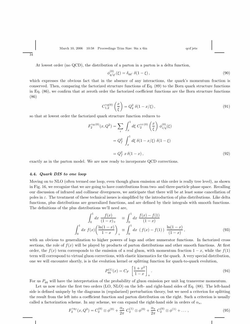
March 10, 2006 10:58 Proceedings Trim Size: 9in x 6in qcd˙jets
34
At lowest order (no QCD), the distribution of a parton in a parton is a delta function,
φ(0)q/q′
(ξ) = δqq′ δ(1 − ξ) , (90)
which expresses the obvious fact that in the absence of any interactions, the quark’s momentum fraction is
conserved. Then, comparing the factorized structure functions of Eq. (89) to the Born quark structure functions
in Eq. (86), we confirm that at zeroth order the factorized coefficient functions are the Born structure functions
(86)
Cγq(0)1,2
(
x
ξ
)
= Q2q δ(1 − x/ξ) , (91)
so that at lowest order the factorized quark structure function reduces to
Fγq (0)2 (x, Q2) =
∑
i
∫ 1
x
dξ Cγi (0)2
(
x
ξ
)
φ(0)i/q(ξ)
= Q2f
∫ 1
x
dξ δ(1 − x/ξ) δ(1 − ξ)
= Q2f x δ(1 − x) , (92)
exactly as in the parton model. We are now ready to incorporate QCD corrections.
4.4. Quark DIS to one loop
Moving on to NLO (often termed one loop, even though gluon emission at this order is really tree level), as shown
in Fig. 16, we recognize that we are going to have contributions from two- and three-particle phase space. Recalling
our discussion of infrared and collinear divergences, we anticipate that there will be at least some cancellation of
poles in ε. The treatment of these technical issues is simplified by the introduction of plus distributions. Like delta
functions, plus distributions are generalized functions, and are defined by their integrals with smooth functions.
The definitions of the plus distributions we’ll need are,∫ 1
0
dxf(x)
(1 − x)+≡∫ 1
0
dxf(x) − f(1)
(1 − x)∫ 1
0
dx f(x)
(
ln(1 − x)
1 − x
)
+
≡∫ 1
0
dx ( f(x) − f(1) )ln(1 − x)
(1 − x), (93)
with an obvious to generalization to higher powers of logs and other numerator functions. In factorized cross
sections, the role of f(x) will be played by products of parton distributions and other smooth functions. At first
order, the f(x) term corresponds to the emission of a real gluon, with momentum fraction 1 − x, while the f(1)
term will correspond to virtual gluon corrections, with elastic kinematics for the quark. A very special distribution,
one we will encounter shortly, is is the evolution kernel or splitting function for quark-to-quark evolution,
P (1)qq (x) = CF
[
1 + x2
1 − x
]
+
. (94)
For us Pqq will have the interpretation of the probability of gluon emission per unit log transverse momentum.
Let us now relate the first two orders (LO, NLO) on the left- and right-hand sides of Eq. (88). The left-hand
side is defined uniquely by the diagrams in (regularized) perturbation theory, but we need a criterion for splitting
the result from the left into a coefficient function and parton distribution on the right. Such a criterion is usually
called a factorization scheme. In any scheme, we can expand the right-hand side in orders of αs,
Fγqf
2 (x, Q2) = C(0)2 ⊗ φ(0) +
αs
2πC
(1)2 ⊗ φ(0) +
αs
2πC
(0)2 ⊗ φ(1) + . . . , (95)
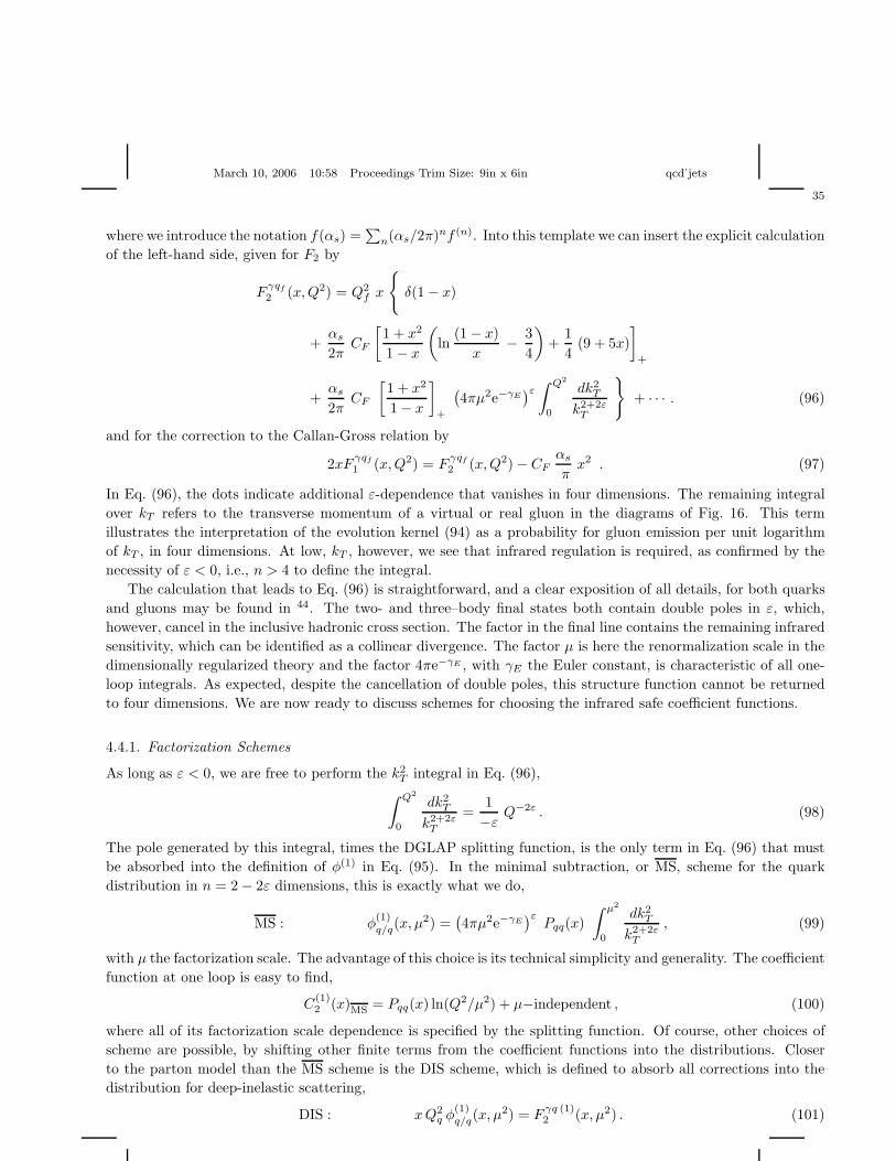
March 10, 2006 10:58 Proceedings Trim Size: 9in x 6in qcd˙jets
35
where we introduce the notation f(αs) =∑
n(αs/2π)nf (n). Into this template we can insert the explicit calculation
of the left-hand side, given for F2 by
Fγqf
2 (x, Q2) = Q2f x
δ(1 − x)
+αs
2πCF
[
1 + x2
1 − x
(
ln(1 − x)
x− 3
4
)
+1
4(9 + 5x)
]
+
+αs
2πCF
[
1 + x2
1 − x
]
+
(
4πµ2e−γE)ε∫ Q2
0
dk2T
k2+2εT
+ · · · . (96)
and for the correction to the Callan-Gross relation by
2xFγqf
1 (x, Q2) = Fγqf
2 (x, Q2) − CFαs
πx2 . (97)
In Eq. (96), the dots indicate additional ε-dependence that vanishes in four dimensions. The remaining integral
over kT refers to the transverse momentum of a virtual or real gluon in the diagrams of Fig. 16. This term
illustrates the interpretation of the evolution kernel (94) as a probability for gluon emission per unit logarithm
of kT , in four dimensions. At low, kT , however, we see that infrared regulation is required, as confirmed by the
necessity of ε < 0, i.e., n > 4 to define the integral.
The calculation that leads to Eq. (96) is straightforward, and a clear exposition of all details, for both quarks
and gluons may be found in 44. The two- and three–body final states both contain double poles in ε, which,
however, cancel in the inclusive hadronic cross section. The factor in the final line contains the remaining infrared
sensitivity, which can be identified as a collinear divergence. The factor µ is here the renormalization scale in the
dimensionally regularized theory and the factor 4πe−γE , with γE the Euler constant, is characteristic of all one-
loop integrals. As expected, despite the cancellation of double poles, this structure function cannot be returned
to four dimensions. We are now ready to discuss schemes for choosing the infrared safe coefficient functions.
4.4.1. Factorization Schemes
As long as ε < 0, we are free to perform the k2T integral in Eq. (96),
∫ Q2
0
dk2T
k2+2εT
=1
−εQ−2ε . (98)
The pole generated by this integral, times the DGLAP splitting function, is the only term in Eq. (96) that must
be absorbed into the definition of φ(1) in Eq. (95). In the minimal subtraction, or MS, scheme for the quark
distribution in n = 2 − 2ε dimensions, this is exactly what we do,
MS : φ(1)q/q(x, µ2) =
(
4πµ2e−γE)ε
Pqq(x)
∫ µ2
0
dk2T
k2+2εT
, (99)
with µ the factorization scale. The advantage of this choice is its technical simplicity and generality. The coefficient
function at one loop is easy to find,
C(1)2 (x)MS = Pqq(x) ln(Q2/µ2) + µ−independent , (100)
where all of its factorization scale dependence is specified by the splitting function. Of course, other choices of
scheme are possible, by shifting other finite terms from the coefficient functions into the distributions. Closer
to the parton model than the MS scheme is the DIS scheme, which is defined to absorb all corrections into the
distribution for deep-inelastic scattering,
DIS : xQ2q φ
(1)q/q(x, µ2) = F
γq (1)2 (x, µ2) . (101)

March 10, 2006 10:58 Proceedings Trim Size: 9in x 6in qcd˙jets
36
In this case,
C(1)2 (x)DIS = xPqq(x) ln(Q2/µ2) + 0 . (102)
Notice that even in DIS scheme, the coefficient inherits the same dependence on the factorization scale as in the
MS scheme. Other schemes, closer to other processes are possible, but nowadays, most calculations are presented
in a minimal scheme.
4.4.2. Using the regulated theory: parton distributions for real hadrons
As we have repeatedly observed, IR-regulated QCD is not the real QCD, but since it differs only in its infrared
sensitivity, we should be able to use infrared safe functions like the Cγq2 ’s even in four dimensions, where we
cannot calculate parton distributions for real hadrons, at least perturbatively. This will enable us to get parton
distributions from real hadrons. Here is how it works:
• Compute F γq2 , F γG
2 (for weak bosons as well).
• Define a factorization scheme; find infrared safe C’s.
• Use these coefficients in the full theory for hadron N ,
F γN2 (x, Q2) =
∑
a=qf ,qf ,G
∫ 1
x
dξ Cγa2
(
x
ξ,Q
µ,µF
µ, αs(µ)
)
φa/N (ξ, µF , αs(µ))
≡ Cγa2 ⊗ φa/N . (103)
• Measure the physical structure functions Fi (not neglecting W and Z boson exchange and neutrino
scattering); then use the known C’s to derive the full set of φa/N for q = q, q, G.
Compared to our discussion above, multiple flavors and structure functions essentially complicate the techni-
calities, but not the logic. Of course, the final step is a highly nontrivial exercise in undoing the convolutions that
relate distributions to observables. Assuming we can carry out this procedure, however, the result is a collection
of parton distributions, φa/N (ξ, µ2), for all partons a (quarks and antiquarks of various flavors, and the gluon) in
the nucleon (proton and neutron). The parton distributions can now be used in any process that factorizes into
distributions times perturbative hard-scattering functions. What we have not explained yet is how to combine
different choices of µF . To that end, we turn to evolution.
5. Evolution
Evolution enables us to determine the Q2-dependence of structure functions, and more than that, to extrapolate
parton distributions from one energy scale to another. It is the cornerstone of predictions at high energy both for
QCD and new physics signals.
For the purposes of this discussion we set the factorization scale equal to the renormalization scale, µF = µ,
so we write Ca
(
x/ξ, Q2/µ2, αs(µ))
. We now choose µ = Q, so that F2, for example, is given for hadron A by
F γA2 (x, Q2) =
∑
a
∫ 1
x
dξ Cγa2
(
x
ξ, 1, αs(Q)
)
φa/A(ξ, Q2) . (104)
The larger is Q, the better the perturbative expansion,
Cγa2
(
x
ξ, 1, αs(Q)
)
=∑
n
(
αs(Q)
π
)n
Cγa2
(n)
(
x
ξ
)
. (105)
To make this work for us, we only need the distribution at µ = Q.
Assuming that we have determined our PDFs at some scale Q0, evolution makes it possible to determine them
at any other scale Q, and hence to determine the structure functions (for example) at any other Q. Our only

March 10, 2006 10:58 Proceedings Trim Size: 9in x 6in qcd˙jets
37
requirement is that both Q and Q0 should be large enough that both αs(Q) and αs(Q0) are small. In particular,
extrapolations to arbitrarily large energies are possible.
We can illustrate these ideas most easily by studying a “nonsinglet” structure function, defined as the difference
between proton and neutron structure functions
F γNSi = F γp
i − F γni , (106)
which may be factorized in terms of a single nonsinglet parton distribution,
F γNS2 (x, Q2) =
∑
a
∫ 1
x
dξ CγNS2
(
x
ξ,Q
µ, αs(µ)
)
φNS(ξ, µ2) . (107)
In this expression, the contributions of gluons and antiquarks have cancelled, and the nonsinglet distribution is a
sum over quark flavors. In fact, these cancellations are relevant only beyond one loop; at one loop CNS2 = CγN
2 .
It is now convenient to take the Mellin transform of Eq. (107), defined by
f(N) =
∫ 1
0
dx xN−1 f(x) . (108)
This has the advantage of reducing convolutions of this kind to products,
f(x) =
∫ 1
x
dy g
(
x
y
)
h(y) → f(N) = g(N) h(N + 1) . (109)
In our case, we find
F γNS2 (N, Q2) = CγNS
2
(
N,Q
µ, αs(µ)
)
φNS(N, µ2) , (110)
where in a slight shift of notation we define φNS(N, µ2) ≡∫ 1
0dξξNφ(ξ, µ2) here.
We now observe that F γNS2 (N, Q2) is physical, so that, as in Eq. (12), it cannot depend on the factoriza-
tion/renormalization scale, µ,
µd
dµF γNS
2 (N, Q2) = 0 . (111)
Applied to Eq. (110), this means that variations in the coefficient function and in the parton distribution must
compensate each other,
µd
dµln φNS(N, µ2) = −γNS(N, αs(µ))
γNS(N, αs(µ)) = µd
dµln CγNS
2 (N, αs(µ)) . (112)
The function γNS(N, αs(µ)) plays the role of a separation constant. It is a function of αs and N only, because
these are the only variables that C and φ hold in common. In particular, it has an infrared safe expansion in αs.
Thus, to get the γ’s we need to know only C’s, which we can get from the infrared regulated theory as above.
The anomalous dimensions γ(N) found in this way, however, enable us to determine the µF dependence of the
parton distributions. For any factorized cross section, we may choose µF at the hard scale in the problem, and
make predictions at high energy based on observations at lower energy.
In summary, the Q-dependence of factorized cross sections is determined by perturbation theory through
evolution. This procedure was how we found out that QCD is the “right” theory for the strong interactions. It
is also the way QCD predicts physics at as-yet unseen scales.

March 10, 2006 10:58 Proceedings Trim Size: 9in x 6in qcd˙jets
38
5.1. Evolution at one loop
We now have all the pieces necessary to derive the consequences of asymptotic freedom and factorization in deep-
inelastic scattering. According to (112), we can compute the anomalous dimensions directly from the coefficient
functions, noting that the answer is the same in either (or any) factorization scheme,
γNS(N, αs) = µd
dµln CγNS
2 (N, αs(Q))
= µd
dµ
(αs/2π) Pqq(N) ln(Q2/µ2) + µ indep.
= −αs
π
∫ 1
0
dx xN−1 Pqq(x)
= −αs
πCF
∫ 1
0
dx
[
(
xN−1 − 1) 1 + x2
1 − x
]
=αs
2πCF
[
4
N∑
m=2
1
m− 2
N(N + 1)+ 1
]
≡ αs
πγ
(1)NS . (113)
We have used the explicit form of the nonsinglet splitting function, Eq. (94). These nonsinglet anomalous di-
mensions are the same as those for the full structure functions, to lowest order. To confirm the integrals the
identity
(1 − xk)/(1 − x) =
k−1∑
i=0
xi (114)
may be helpful.
Having done the work, it’s just a small step to some extraordinary physics predictions e. Going back to Eq.
(112), the very anomalous dimensions computed from the NLO coefficient functions control the factorization scale
dependence of the parton distributions,
µd
dµφNS(N, µ2) = −γNS(N, αs(µ)) φNS(N, µ2) , (115)
The solution to this equation is an exponential, where the exponent is an integral over the scale appearing in the
running coupling,
φNS(N, µ2) = φNS(N, µ20) exp
[
−1
2
∫ µ2
µ20
dµ′2
µ′2γNS(N, αs(µ))
]
. (116)
Of course, we can evaluate this expression for any theory, once we determine the anomalous dimensions and
the running of the coupling as above. If (the generic case) the theory is not asymptotically free, the coupling
increases rather than decreases with µ′, on the basis of its one-loop beta function. At the same time the anomalous
dimensions, the analogs of γ(1)NS(N, αs), remain positive. Once the coupling is large, of course, it may no longer
be possible to use the one-loop anomalous dimensions, and it is still possible that the coupling constant might
approach a finite constant (a fixed point) due to higher-order terms in the beta function. This, however, would
predict violations of scaling by a power in µ, and hence in Q 17. In contemporary terms, for such theories the
eAs the written form of these lectures were being prepared, the 2004 Nobel Prize honoring the discovery of asymptotic freedom wasawarded. The field theoretic explanation of scaling and scale breaking, in much the same manner as presented here, was the originallink of QCD to experiment and remains one of its strongest links to this day

March 10, 2006 10:58 Proceedings Trim Size: 9in x 6in qcd˙jets
39
parton distributions decrease rapidly in µ, and hence the moments of the structure functions decrease very strongly
with Q. In physical terms, a decrease in the moments corresponds to a rapid shift of the parton distributions
from larger to smaller x as Q increases. This was the paradox of scaling in 1973: all known field theories seemed
to predict too much radiation for partons to retain their momentum fractions x at large Q2.
In QCD, of course, asymptotic freedom changes this. The QCD coupling (11) decreases with scale. We can
perform the µ′ integral in the exponent of (116) easily, to get
φNS(N, Q2) = φNS(N, Q20)
(
ln(Q2/Λ2QCD)
ln(Q20/Λ2
QCD)
)−2γ(1)N /b0
, (117)
which is also often written as
φNS(N, Q2) = φNS(N, Q20)
(
αs(Q20)
αs(Q2)
)−2γ(1)N /b0
. (118)
Scale breaking has not disappeared, but it is now logarithmic, and hence very mild once Q is significantly larger
than the scale ΛQCD. This establishes both the consistency of QCD with the parton model, and a constellation
of predictions for improvements to the parton model, which have been confirmed in the intervening years.
The scaling violation predictions of QCD are easiest to compute via moments of the parton distributions as
above. For numerical evaluation, however, it is often more convenient to invert the moments, which takes the
simple rate equation for the parton density in (112) back to a convolution
µd
dµφNS(x, µ2) =
∫ 1
x
dξ
ξPNS(x/ξ, αs(µ)) φNS(ξ, µ2) , (119)
in terms of the very same splitting function,∫ 1
0
dx xN−1 Pqq(x, αs) = −γqq(N, αs) + · · · =
∫ 1
0
dx xN−1 PNS(x, αs) + . . . , (120)
where again, the nonsinglet and quark-quark splitting functions are the same to lowest order. Equation (119)
commonly referred to as the DGLAP evolution equation 46, also provides a nice physical interpretation of evolution,
as a sequence of radiation processes. At each such step, the parton momentum fraction ξ is degraded to x < ξ,
in an essentially probabalistic manner.
5.2. Beyond nonsinglets
The generalization of these results to the full system of parton distributions is simple, at least in principle. As long
as the sequential radiation processes that drive evolution involve only gluons, the evolutions of individual quark
flavors are independent. The (singlet) structure functions for individual hadrons, however, receive contributions
from fermionic as well as gluonic radiation, which couples the evolutions of all the quarks, antiquarks and the
gluon. Compared to Eq. (119), the only change is that the nonsinglet splitting function is replaced by a matrix
Pba, each element of which describes the production of partons of flavor b from those of flavor a,
µd
dµφb/A(x, µ2) = −
∑
b=q,q,G
∫ 1
x
dξ
ξPba(ξ, αs(µ)) φa/A(ξ, µ2) , (121)
or in moment space
µd
dµφb/A(N, µ2) = −
∑
b=q,q,G
γba(N, αs(µ)) φa/A(N, µ2) , (122)
in terms of a matrix of anomalous dimensions, γba(N). Of special interest is the low-x behavior of Pgg(z) ∼ 1/z,
which corresponds to γgg(N) ∼ 1/(N −1). For N ∼ 1 moments, then, the effects of evolution can be large, simply

March 10, 2006 10:58 Proceedings Trim Size: 9in x 6in qcd˙jets
40
because large anomalous dimensions raise the logarithms corresponding to those in (118) above to a high power.
The strong scale-breaking effects of such terms in the anomalous dimensions are clearly seen in the data of Fig.
17. The systematic study of low-x evolution is a subfield in its own right, which starts with the famous BFKL
equation 47, which organizes the leading logarithms in x at each order of αs. An introduction can be found in
Ref. 35, and a summary of recent highlights in Ref. 48.
5.3. Summary
Here is a summary our discussion of factorization and evolution. In the parton model, φa/A(x) denotes the density
of partons a with momentum fraction x, a distribution that is assumed to be quantum-mechanically independent
of the hard scattering at momentum transfer Q, and hence may be treated as an independent probability. In
QCD, φa/A(x, µ) represents the same density, but only of partons with transverse momentum ≤ µ, as illustrated
by the integral of Eq. (96). It is only these partons whose production may be considered incoherent with the hard
scattering.
If there were a maximum transverse momentum Q0 for partons in the nucleon, φ(x, Q0) would freeze for
µ ≥ Q0, and the theory would revert to the parton model above that scale. This is never the case, however, in
a renormalizable field theory, and scale breaking measures the change in the density as the maximum transverse
momentum increases. Of course, the structure functions and cross sections that we compute still depend on our
choice of µ through uncomputed higher orders in C and evolution. At present, evolution for DIS is routinely
implemented fully up to NLO, which requires order α2s in the splitting functions Pab. This formalism can suc-
cessfully describe the behavior of structure functions over a wide range of x, as illustrated by Figs. 14 and 17.
The full splitting functions up to α3s have just become available within the past year 49, and the development of
Figure 17. DIS data at low x, compared to fits from Ref. 45.
a phenomenology at NNLO is underway 50.

March 10, 2006 10:58 Proceedings Trim Size: 9in x 6in qcd˙jets
41
6. Applications and Extensions
In this final section, we will touch on a (very incomplete) subset of the generalizations of the jet and DIS analyses
we have just described, including factorization for hadron-hadron scattering, the basis of all-orders factorization
proofs and of resummations, and a few current areas of progress relevant to the LHC program.
6.1. Factorized hadron hadron cross sections
Space does not allow an extensive description of the application of factorization and evolution to hadron hadron
scattering 30,35, but even a cursory description shows the utility of these techniques. The factorization formalism
can be extended to the semi-inclusive production of heavy particles or systems of jets, labeled F , of mass Q.
Indeed, the decay of a system of heavy particles, be it a top quark pair or SUSY signal, usually results in hadronic
jets. An essential element of new-particle searches is to tease the signals of these decays out of the QCD and
electroweak background.
The production of final-state F requires the short-distance collisions of a parton from each hadron, and the same
pinch surface and power counting analysis as for e+e− annihilation and DIS shows that the entire leading power
in Q comes from only a single (physical) parton from each hadron 30. The essential requirement for factorization
is once again that we sum over states involving the emission of soft particles and/or the rearrangement of collinear
radiation. It is important that the definition of the semi-inclusive final state not involve any scales much smaller
than Q, the mass of the observed final state, because the largest corrections will generally be an inverse power of
the smallest such scale.
A factorized cross section for hadron-hadron scattering describes the production of final states by a direct
generalization of DIS factorization, as a convolution of two parton distributions with a hard-scattering function,
σAB→F (Q)(Q) =∑
a,b=q,q,G
∫ 1
0
dx dy φa/A(x, µ) φb/B(y, µ) σab→F (Q)(xpA, ypB, Q, µ, αs(µ))
×θ(xypA · pB − Q2) , (123)
where we have exhibited a theta function to emphasize the requirement that the partonic system has sufficient
energy to produce system F of mass Q. As usual, the hard-scattering function σ begins at lowest order with a
Born cross section, and depends on the choice of µ through uncomputed higher orders.
An illustrative O(αs) (NLO) hard-scattering cross section is the quark-antiquark annihilation cross section
σqq for the Drell-Yan process (qq → γ or Z → `+`−), given in MS by
σ(1)qq = σBorn(Q2) CF
(
αs(µ)
π
)
Pqq(z) ln
(
Q2
µ2
)
+ 2(1 + z2)
[
ln(1 − z)
1 − z
]
+
−[
(1 + z2) ln z]
(1 − z)+
(
π2
3− 4
)
δ(1 − z)
, (124)
where z = Q2/xaxbS with√
S the total center of mass energy squared, and where σBorn describes the electroweak
annihilation of q q. We see again a plus distribution, whose presence reflects the cancellation of real and virtual
soft gluons.
A perturbative prediction for this process, based on factorization, is compared to data at high energy (γ and
Z), is shown in Fig. 18 from CDF at the Tevatron, The peak due to the Z is clearly visible, and indeed this was
the way the Z was first directly seen. Also shown is data for the forward-backward asymmetry associated with the
parity-violating predictions of the standard model, and some extenstions of it. Notice that this asymmetry, with
or without a new physics signal, is calculable precisely because it is part of the hard scattering function. Such
tests, for signals of new states or violations of symmetries, are the prototypes for the detection of new physics in
hadronic scattering.

March 10, 2006 10:58 Proceedings Trim Size: 9in x 6in qcd˙jets
42
Figure 18. Drell-Yan data from the Tevatron 51.
The successes and remaining uncertainties of predictions based on factorized perturbation theory are well
illustrated by the data for inclusive high-pT jet cross sections, based on formulas that are analogous to those for
Drell-Yan, but (much, much) more elaborate even at NLO 52. The data track perturbative predictions over many
orders of magnitude, but even between the two Fermilab experiments, differences in analysis of the still-preliminary
data 53 show that there is still work to be done.
The LHC program for the discovery of new particles and/or new strong interactions at high energy relies
heavily on the factorization formalism. So long as it involves heavy states, each prediction of an extension of the
standard model appears in the hard scattering function of the factorized cross section. The parton distributions
are the same as those observed in DIS at lower energy, now extrapolated by evolution.
6.2. Factorization proofs and matrix elements
In the previous section we have made extensive use of factorization for the DIS structure functions, and now we
have seen how they generalize to hadronic collisions. Let us come back briefly to the proof of the forms (103) for
the former and (123) for the latter.
For deep-inelastic scattering, there are a number of ways to provide a proof. One way is based on the light-cone
expansion of Eq. (14), and is most conveniently formulated in terms of moments.
Alternatively, we may begin wiith the pinch surfaces and hence physical pictures for the process eN → e+ X ,
where we assume a large momentum transfer, Q. These are shown in Fig. 21, and generally involve jets in the
final state, in addition to collinear fragments of the incoming nucleon. The figure shows a single parton, labeled
i combining with the off-shell photon of labeled q to produce a final state. Physical pictures with more collinear

March 10, 2006 10:58 Proceedings Trim Size: 9in x 6in qcd˙jets
43
[GeV/c]TP0 50 100 150 200250 300 350 400450 500
Da
ta /
NL
O (
CT
EQ
61
)
0.5
1
1.5
2
2.5
3
CDF Run II Preliminary
D=0.5 - 0.1<|Y|<0.7TKSystematic ErrorsNLO Uncertainties
/2MAXT = PFµ = RµNLO: JETRAD
No Had. / Und. Event Correction
-1L = 145 pb
[GeV/c]TP0 100 200 300 400 500 600 700
Da
ta /
NL
O (
CT
EQ
61
)
0
1
2
3
4
5
6
7
8CDF Run II Preliminary
D=0.7 - 0.1<|Y|<0.7TKSystematic ErrorsNLO Uncertainties
-1L = 145 pb
/2MAXT = PFµ = RµNLO: JETRAD
No Had. / Und. Event Correction
Figure 19. Recent preliminary CDF jet data 53. The data is presented here as the ratio of the difference between data and the NLOprediction, normalized to the prediction. As the following figure shows, the absolute value of the data is changing by many orders ofmagnitude over this range.
[GeV/c]Tp100 200 300 400 500 600
[p
b /
(G
eV
/c)]
⟩ T
/ d
pσ
d⟨
10-4
10-3
10-2
10-1
1
10
102
103
[GeV/c]Tp100 200 300 400 500 600
[p
b /
(G
eV
/c)]
⟩ T
/ d
pσ
d⟨
10-4
10-3
10-2
10-1
1
10
102
103
|y| < 0.5 , Cone R=0.7
Systematic uncertainties
NLO (JETRAD) CTEQ6MmaxT = 0.5 pRµ = Fµ=1.3, sep R
Run II preliminaryOD
-1 = 143 pbintL
[GeV/c]Tp100 200 300 400 500 600
da
ta /
th
eo
ry
0
1
2
3
4
5
6
[GeV/c]Tp100 200 300 400 500 600
da
ta /
th
eo
ry
0
1
2
3
4
5
6
[GeV/c]Tp100 200 300 400 500 600
|y| < 0.5Systematics uncertaintiesPDF uncertainties
Run II preliminaryOD
-1 = 143 pbintL
Cone R=0.7
maxT = 0.5 pRµ = Fµ=1.3, sep R
NLO (JETRAD) CTEQ6M
Figure 20. Recent preliminary D0 jet data 53.
partons are possible. As in the discussion of jet production in e+e− annihilation above, at leading power in Q,
they can be only unphysically-polarized gluons (in covariant gauges). It is worth noting that the requirement
of a physical picture implies that the momentum fraction of the parton that initiates the hard scattering obeys
1 > ξ > x, for much the same reasons as in our low-order examples above; all the partons in a jet or hadron must
be moving in the same direction. For the inclusive DIS cross section, we sum over all final states, and information
on the time development of the final state jets is lost, just as in the total e+e− annihilation cross section. For DIS,
however, the initial-state evolution that provides the “active” parton (the one that initiates the hard scattering)
remains.
The DIS argument regarding the sum over states has the same content as the optical theorem for DIS: the
total γ∗ p cross section is related to the γ∗p forward scattering amplitude. In terms of the hadronic tensor of Eq.

March 10, 2006 10:58 Proceedings Trim Size: 9in x 6in qcd˙jets
44
Figure 21. Pinch surface for DIS.
(81), this can be written as
Wµν = 2 Im Tµν , (125)
where the tensor Tµν is the expectation of the time-ordered product of currents,
Tµν =i
8π
∫
d4x eiq·x < N(p)| T Jµ(x)Jy(0) |N(p) > . (126)
Because of the optical theorem, the long-distance behavior of the hadronic tensor is specified by the pinch surfaces
of this matrix element, which can be described as the amplitude for forward Compton scattering of a nucleon by
an off-shell photon. The pinch surfaces in this case are much simpler than those for individual final states. The
requirement of a physical picture shows that no jets are possible aside from the “forward” jet of fragment partons
from the incoming nucleon, which reform after the hard scattering into an outgoing nucleon of the same total
momentumf . The hard scattering is reduced to a point, because, as in the e+e− case, on-shell particles that travel
a finite distance from the hard scattering can never recombine. At the pinch surface, the hard-scattering function
H depends only on the non-vanishing longitudinal component ξp of the active parton’s momentum. Once we
have reached this stage, the remainder of the factorization argument is a systematic disentangling of the upper
and lower parts of Fig. 22, in terms of color, spin and momentum. A hierarchy of subtractions 30 effects this
separation.
The parton distributions factorized in this mannner take the form of the expectation values of operators
relatively on the light cone. To specify these matrix elements, it is convenient to choose the momentum of
fA related physical off-diagonal amplitude 9, γ∗+p → γ+p called deeply-virtual Compton scattering, offers complementary informationon hadronic structure, and may also be factorized 54.

March 10, 2006 10:58 Proceedings Trim Size: 9in x 6in qcd˙jets
45
Figure 22. Pinch surface for forward Compton scattering.
incoming nucleon h in the plus light-cone direction, and to define an opposite-moving light-like vector, nµ = δµ−.
The parton distribution is then
φq/h(ξ, µ2) =1
2
∑
σ
∫ ∞
−∞
dy−
2πe−iξp+y−
< h(p, σ) | q(0+, y−,0⊥)1
2n · γ q(0) | h(p, σ) > , (127)
where the average over spins for an unpolarized cross section is exhibited. This matrix element can be defined
in n · A = 0 = A+ gauge. Choosing the incoming hadron as a quark, and computing (127) at order αs, we
find precisely the MS quark distribution discussed in Sec. 4 above. The formalism can readily be extended to
covariant gauges, and the matrix element made gauge invariant, by connecting the quark operators with ordered
exponentials (also known as nonabelian phases, gauge links and Wilson lines),
q(y−) n · γ q(0) → q(y−)P exp
[
ig
∫ y−
0
dl n · A(lnµ)
]
n · γ q(0) . (128)
These and related forms of parton distributions, including their generalizations to transverse momentum distri-
butions, were discussed extensively in Ref. 55.
An extensive discussion of proofs of perturbative factorization for semi-inclusive hard scattering cross sections
in hadron hadron scattering 56 may be found in 30, with additional comments in Ref. 34. Here, I will only recall
a few of the heuristic arguments.
The essential challenge when there are two hadrons in the initial state is to show the universality of the parton
distribution functions between DIS and hadron-hadron scattering. Consider a Drell-Yan cross section, in which a
quark from one hadron annihilates with an antiquark from the other to form a virtual photon, W or Z (generic
mass Q). We’ll think of a range in kinematics where the quark and antiquark carry a large fraction x of their
parent hadron’s momentum, so that there is no confusion about which of the pair comes from which hadron.
It is natural to wonder whether, with two hadrons in the initial state the color fields of each hadron might
permeate the other prior to the annihilation, modifying the colors, or even transverse momenta, of the annihilating
pair in such a way as to increase or decrease their amplitude for the annihilation. A proof of factorization must

March 10, 2006 10:58 Proceedings Trim Size: 9in x 6in qcd˙jets
46
show that such effects decrease as a power of the pair invariant mass, Q. The technical arguments rely on the
formalism we have developed above in Sec. 3. The summation over final states that defines the semi-inclusive
cross section results in an expression for which the only pinch surfaces that remain logarithmic in their power
counting after the sum over final states are in one-to-one correspondence with those found in the inclusive DIS
cross section, separately for the two hadrons. The hadron-hadron cross section is then factorizable in the same
manner as deep-inelastic scattering.
The physical reason for this rather simple result is not far to seek. The Lorentz contracted fields of incident
particles do not overlap until the moment of the scattering 57. As a result, initial-state interactions that couple
the two hadrons disappear at high enough energies. All remaining initial-state interactions are internal to the
hadrons, and are specified by the same parton densities as in deep-inelastic scattering. It is a matter of relativistic
causality: as the relative velocities of the two hadrons approaches the speed of light, they are unable to exchange
signals of any kind. Correspondingly, the annihilation process itself (or other hard-scattering reaction) must also
occur on a very short time scale, and final-state interactions, after the hard scattering, are simply too late to
affect large momentum transfer and/or creation of the heavy particle(s).
6.3. Resummations: a closer look at the final state
These lectures have concentrated on applications of asymptotic freedom, infrared safety and factorization in semi-
inclusive cross sections with only a single hard scale. A closer look at the final state, in terms of shape functions,
generally introduces another scale, as noted in Sec. 3.5. The second scale may be perturbative, but ratios of
the two perturbative scales may be large at any fixed order in perturbation theory. For example, in the limit of
low jet masses in Eq. (74) (thrust goes to 1) or of low angularities ea in Eq. (77), these corrections build up as
(1/M2Ji)αn
s ln2n−1(MJi/Q) and (1/ea)αns ln2n−1 ea, respectively. Note the overall additional power singularity at
zero jet mass in each case.
In cases like jet masses and angularities, we can control these large corrections to all orders in perturbation
theory, a process known as resummation. Resummations, like evolution in DIS, can usually be derived from
a factorization formula, as in Eq. (112) for evolution. We can illustrate this process for the angularities (77).
Details are given in Ref. 40, but the basic observations are simple enough. In the limit of small ea, the final state
consists of two well-collimated jets, accompanied by very soft wide-angle radiation. The soft radiation cannot
resolve the internal structure of the jets, and is equivalent to the soft radiation emitted by a pair of point-like
recoil-less sources in the fundamental representation of the gauge group (quark and antiquark representations).
In this limit, the cross section factorizes as shown in Fig. 23. Here each of the individual factors can be given a
field-theoretic interpretation, an example being the functions associated with the jets,
Jµq (p · ξ, ea, µ) =
(2π)6
Nc
∑
N
Tr
[
γµ⟨
0∣
∣
∣Φ
(q)ξ
†(0,−∞; 0)q(0)∣
∣
∣N⟩⟨
N∣
∣
∣q(0)Φ
(q)ξ (0,−∞; 0)
∣
∣
∣0⟩
]
× δ(ea − ea(N, a)) δ3 (pJ − p(N)) . (129)
As in the case of the matrix element that defines the quark distribution (127) with (128), we have introduced an
ordered exponential in the direction of the vector ξ to make the jet function gauge-invariant. We also need to
introduce a factorization scale, µ, to separate the hard, jet and soft functions. Both the scale µ and the vector
ξν are artifacts of the factorization; neither appears in the cross section itself, but the factorization is valid up
to positive powers of ea, which is small. The factorized cross section therefore obeys two equations, analogous to
(12),
µdσ
dµ= 0
ξα dσ
dξα= 0 . (130)

March 10, 2006 10:58 Proceedings Trim Size: 9in x 6in qcd˙jets
47
Figure 23. Factorization near the two-jet limit.
The solutions to these equations are a generalization of the evolution of parton distributions, and as in that
case, they are most simply presented in a transform space, in this case a Laplace transform with respect to the
angularities. The limit of small ea corresponds directly to large values of the transform variable ν, dependence
on which exponentiates,
σ(ν, Q, a) =
∫
0
dea e−νea σ(ea, Q, a) = eE(ν,Q,a) , (131)
where the exponent E(ν) is given by
E(ν, Q, a) = 2
1∫
0
du
u
[ uQ2∫
u2Q2
dp2T
p2T
Aq (αs(pT ))(
e−u1−aν(pT /Q)a − 1)
+1
2Bq
(
αs(√
uQ))
(
e−u(ν/2)2/(2−a) − 1)
]
. (132)
In the exponent, the presence of two integrals reflects the two consistency equations (130), and the functions
Aq, Bq are infrared-safe anomalous dimensions. In particular A = (αs/π)CF + . . . also appears in Pqq(x, αs) =
A(αs)/(1 − x) + . . . , and is now known to three loops 49. For quark jets, B = (αs/π)(3CF /2) + . . . is somewhat
more process dependent. Expressions like this, with a double integral over the running coupling, were first derived
in studies of the transverse momentum distribution for the Drell-Yan cross section, especially as developed by
Collins and Soper 58 and Sen 59.
The inversion of the transform leads to distributions of the sort shown in Fig. 24 for the mass of the “heavy”
jet in e+e− annihilation, and for the distribution of Z transverse momenta at the Tevatron in Fig. 25.
In both figures, the cross section has a peak very near the kinematic configuration of elastic scattering: for
e+e−, ea = 0, corresponding to a quark-pair final state, and QT = 0, corresponding to the production of a Z in
Born approximation. In both cases, the effect of gluonic radiation is to turn a delta function distribution into
one that rises to a peak near the elastic limit, and then slowly falls off away from that limit. The tail of the
distribution away from the peak is given by low-order perturbation theory, and the position of the peak can be
calculated perturbatively as well. Nevertheless, the bulk of the inclusive cross section is concentrated near the
peak, and in this region, nonperturbative corrections are suppressed only by powers off 1/(eaQ), rather than

March 10, 2006 10:58 Proceedings Trim Size: 9in x 6in qcd˙jets
48
0 0.1 0.2 0.3
ρ
0
10
20
30
1/
totd
dAleph
Delphi
L3
'Exclusive limit'
Figure 24. Heavy jet distribution. From Ref. 60.
66 < Q < 116 GeV
CDF
Exclusive Limit
Resum
Resum+power
Figure 25. Transverse momentum distribution for the Z at the Tevatron. From Ref. 61.
1/Q 37. This effect can be inferred directly from the Eq. (132) 33. A sketch of the transition from resummed
perturbation theory to nonperturbative power corrections can be found in Ref. 62.
March 10, 2006 10:58 Proceedings Trim Size: 9in x 6in qcd˙jets
49
6.4. Higher orders
Predictions based on factorized cross sections in perturbative QCD require both hard-scattering functions and
parton distributions. It is an understatement that making progress on both of these topics is nontrivial in almost
every case of practical interest. The past few years, however, have seen important progress, through a growing
mastery over higher order corrections, and through the improved determination of parton distributions from a
growing set of data. Certainly, the coming of the LHC has helped drive much of this work, but their own internal
logic, and the special challenges these projects pose, have surely provided strong motivations as well.
6.4.1. Toward a two-loop phenomenology
In effect, the transition from leading order to next-to-leading order accuracy at the level of jet cross sections took
about a decade, and a similar time scale will have been necessary to realize, for example, full NNLO jet cross
sections in time for the LHC. Given the experimental value of αs(mZ) ∼ 1.2 63, hard-scattering cross sections at
the order of α2s(MZ) have a nominal accuracy in the per cent range. For some semi-inclusive cross sections at
momentum transfers in the hundreds of GeV, this is also the scale of many nonperturbative corrections, including
those associated with uncertainties in the parton distribution functions (see below). Percent accuracy is probably
attainable for benchmark cross sections, as a foundation from which to understand the complex final states
associated with the decay of new, heavy particles, and the QCD backgrounds to them.
The development of a NNLO phenomenology is following the pattern of NLO. For some time, fully inclusive
NNLO cross sections for e+e− annihilation, DIS, and Drell-Yan annihilation (including Higgs production) have
been available 64. More complex is the combination of final states in e+e− jet cross sections, and even more so
the factorization necessary for jet cross sections in hadron-hadron scattering. Even at NLO the state of the art is
4-jet cross sections for e+e−, and up to 3 jets at hadron colliders 52.
Within the last few years, the elements necessary for factorized NNLO cross sections are beginning to be
assembled in earnest. Progress has been made in NNLO e+e− jet cross sections 65, while the amplitude at O(α3s)
has become available for three jets. The past few years have also seen the first NNLO two-loop S-matrix elements
for the 2 → 2 scattering 66, an essential step toward jet cross sections in hadron-hadron scattering. Important
progress is also ongoing toward organizing the singular integrals over phase space 67. Equally significant is the
calculation of NNLO splitting functions, the fruit of a decade-long program 49.
Many of these acheivements have required developing new methods in the organization of large numbers of
Feynman diagrams 68 often involving astronomical numbers of terms. Hope springs eternal that new mathematical
insights 69 may simplify the road ahead, at least for the calculation of on-shell amplitudes.
6.4.2. Parton distributions: global fits and uncertainties
The determination of parton distributions is a bootstrap process. As described in Sec. 3, they must be abstracted
from the comparison of sets of data to factorized cross sections, with hard-scattering functions computed up to
a given order. For the past ten years, the calculation has been at the level of NLO. Any set of distributions
determined this way is limited not only by the accuracy of the calculations, but also by the sensitivity of the data
to given distributions. For example, in DIS, photons or weak vector bosons couple to the quarks at zeroth order,
while the gluons get into the act only at order αs in the hard scattering. Naturally, we might expect DIS to be less
informative about gluons than about quarks, and we look for other processes, like jet production, which can be
more directly sensitive to the gluon distribution. Other cases where new data have provided new and sometimes
surprising insights concern the ratios of d-quark and u-quark distributions from W± asymmetry measurements
at the Tevatron collider 51, and of the d and u from fixed-target Drell-Yan data 70.
In any case, once a model set of PDFs has been produced, it provides predictions for other factorizable cross
sections. As new data become available, it may require us to modify existing models to incorporate new features.
This feedback procedure has evolved into the approach of “global” fits, which try to use the best available data
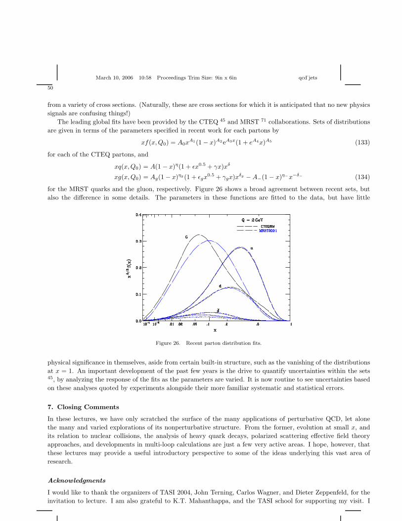
March 10, 2006 10:58 Proceedings Trim Size: 9in x 6in qcd˙jets
50
from a variety of cross sections. (Naturally, these are cross sections for which it is anticipated that no new physics
signals are confusing things!)
The leading global fits have been provided by the CTEQ 45 and MRST 71 collaborations. Sets of distributions
are given in terms of the parameters specified in recent work for each partons by
xf(x, Q0) = A0xA1(1 − x)A2eA3x(1 + eA4x)A5 (133)
for each of the CTEQ partons, and
xq(x, Q0) = A(1 − x)η(1 + εx0.5 + γx)xδ
xg(x, Q0) = Ag(1 − x)ηg (1 + εgx0.5 + γgx)xδg − A−(1 − x)η−x−δ− (134)
for the MRST quarks and the gluon, respectively. Figure 26 shows a broad agreement between recent sets, but
also the difference in some details. The parameters in these functions are fitted to the data, but have little
Figure 26. Recent parton distribution fits.
physical significance in themselves, aside from certain built-in structure, such as the vanishing of the distributions
at x = 1. An important development of the past few years is the drive to quantify uncertainties within the sets45, by analyzing the response of the fits as the parameters are varied. It is now routine to see uncertainties based
on these analyses quoted by experiments alongside their more familiar systematic and statistical errors.
7. Closing Comments
In these lectures, we have only scratched the surface of the many applications of perturbative QCD, let alone
the many and varied explorations of its nonperturbative structure. From the former, evolution at small x, and
its relation to nuclear collisions, the analysis of heavy quark decays, polarized scattering effective field theory
approaches, and developments in multi-loop calculations are just a few very active areas. I hope, however, that
these lectures may provide a useful introductory perspective to some of the ideas underlying this vast area of
research.
Acknowledgments
I would like to thank the organizers of TASI 2004, John Terning, Carlos Wagner, and Dieter Zeppenfeld, for the
invitation to lecture. I am also grateful to K.T. Mahanthappa, and the TASI school for supporting my visit. I

March 10, 2006 10:58 Proceedings Trim Size: 9in x 6in qcd˙jets
51
feel lucky to have had the opportunity to interact with the TASI 2004 students, and I thank them for the interest
they showed in the subjects discussed here. This work was supported in part by the National Science Foundation,
grants PHY-0098527 and PHY-0354776.
References
1. A. Pais, Inward Bound (Oxford University Press, New York, 1986), Chapter 19.2. Review of Particle Properties, S. Eidelman et al. (Particle Data Group) Phys. Lett. 592, 1 (2004).3. E. Fermi and C.N. Yang, Phys. Rev. 76 (1949) 1739.4. J.H. Schwarz, Phys. Rept. 8, 269 (1973)5. R. Hofstadter and R.W. McAllister, Phys. Rev. 98, 217 (1955).6. M. Perl, High Energy Hadron Physics (Wiley-Interscience, New York, 1974).7. M.K. Jones et al., Phys. Rev. Lett. 84, 1398 (2002), O. Gayou et al., Phys. Rev. Lett. 88, 092301 (2002).8. S.J. Brodsky and G.P. Lepage, in Perturbative Quantum Chromodynamics, ed. A.H. Mueller (World Scientific, Singa-
pore, 1989), p. 93.9. X. Ji, J. Phys. G24, 1181 (1998) hep-ph/9807358.
10. R.P. Feynman, Phys. Rev. Lett. 23, 1415 (1969).11. D.J. Gross and F. Wilczek, Phys. Rev. D8, 3633 (1973);
H.D. Politzer, Phys. Rept. 14, 129 (1974).12. H. Fritzsch, M. Gell-Mann and H. Leutwyler Phys. Lett. B47, 365 (1973).13. C.N. Yang and R.L. Mills, Phys. Rev. 96, 191 (1954).14. S. Weinberg, Phys. Rev. Lett. 31, 494 (1973).15. J.D. Bjorken, Phys. Rev. 179, 1547 (1969).16. R.A. Brandt and G. Preparata, Nucl. Phys. B27, 541 (1971);
Y. Frishman, Phys. Rev. Lett. 25, 966 (1970).17. N. Christ B. Hasslacher and A.H. Mueller, Phys. Rev. D6, 3543 (1972).18. B. Edwards et al., Phil. Mag. 3, 237 (1957).19. S.D. Drell, D.J. Levy and T.M. Yan, Phys. Rev. D1, 1617 (1969).20. G. Hanson et al., Phys. Rev. Lett. 35, 1609 (1975).21. G. Sterman and S. Weinberg, Phys. Rev. Lett. 39, 1436 (1977).22. H.D. Politzer, Phys. Lett. B70, 430 (1977);
A. De Rujula, John R. Ellis, E.G. Floratos and M.K. Gaillard, Nucl. Phys. B138, 387 (1978).23. F. Bloch and A. Nordsieck, Phys. Rev. 52, 54 (1937);
D.R. Yennie, S.C. Frautschi and H. Suura, Annals Phys. 13, 379 (1961).24. T. Kinoshita, J. Math. Phys. 3, 650 (1962);
T.D. Lee and M. Nauenberg, Phys. Rev. 133, B1549 (1964).25. G. ’t Hooft and M.J.G. Veltman, Nucl. Phys. B44, 189 (1972); and in Louvain 1973, Particle Interactions At Very
High Energies, Part B, New York 1973, 177 and CERN report - CERN 73-9;J.F. Ashmore, Lettere al Nuovo Cim. 4, 289 (1972);C.G. Bollini and J.J. Giambiagi, Nuovo Cim. Ser, 1112B, 20 (1972).
26. S. Coleman and R.E. Norton, Nuorvo Cim. Ser. 10 38, 438 (1965).27. G. Sterman, Phys. Rev. D17, 2773; 2789 (1978).28. L.D. Landau, Nucl. Phys. 13, 181 (1959).29. J.M.F. Labastida and G. Sterman, Nucl. Phys. B254, 425 (1985).30. J.C. Collins, D.E. Soper and G. Sterman, in Perturbative quantum chromodynamics, ed. A.H. Mueller (World Scientific,
Singapore, 1989), p. 1, hep-ph/0409313.31. C.W. Bauer, S. Fleming and M.E. Luke, Phys. Rev. D63, 014006 (2001) hep-ph/0005275;
C.W. Bauer, S. Fleming, D. Pirjol and I.W. Stewart, light Phys. Rev. D63, 114020 (2001) hep-ph/0011336;C.W. Bauer and I.W. Stewart, Phys. Lett. B516, 134 (2001) hep-ph/0107001;C.W. Bauer, D. Pirjol and I.W. Stewart, Phys. Rev. D65, 054022 (2002) hep-ph/0109045.
32. G. Sterman, Phys. Rev. D19, 3135 (1979).33. G.P. Korchemsky, at 33rd Rencontres de Moriond and 3rd Workshop on Continuous Advances in QCD (QCD 98),
Minneapolis, MN, hep-ph/9806537;G.P. Korchemsky and G. Sterman, Nucl. Phys. B555 335 (1999) hep-ph/9902341.
34. G. Sterman, in QCD and Beyond, ed. D.E. Soper (World Scientific, Singapore, 1996), 1995 TASI lectures, hep-
March 10, 2006 10:58 Proceedings Trim Size: 9in x 6in qcd˙jets
52
ph/9606312.35. R.K. Ellis, W.J. Stirling and B.R. Webber, QCD and collider physics (Cambridge University Press, 1996).36. G. Blazey et al., in Batavia 1999, QCD and weak boson physics in Run II p. 47, hep-ex/0005012.37. M, Dasgupta and G.P. Salam, J. Phys. G30, R143 (2004) hep-ph/0312283.38. E. Farhi, Phys. Rev. Lett. 39, 1587 (1977).39. S. Catani, G. Turnock, B.R. Webber, Phys. Lett. B295, 269 (1992);
Yu.L. Dokshitzer, A. Lucenti, G. Marchesini and G.P. Salam, JHEP 9801, 011 (1998) hep-ph/9801324.40. C.F. Berger, T. Kucs and G. Sterman, Phys. Rev. D68 014012 (2003) hep-ph/0303051.41. DRESSED C.F. Berger and L. Magnea, hep-ph/0407024.42. OPAL Collaboration (G. Abbiendi et al.), Eur. Phys. J. C16, 185 (2000) hep-ex/0002012 .43. C.G. Callan and D.J. Gross, Phys. Rev. Lett. 22, 156 (1969).44. G. Altarelli, R.K. Ellis and G. Martinelli, Nucl. Phys. B157, 461 (1979).45. J. Pumplin et al., JHEP 0207, 012 (2002), hep-ph/0201195.46. G. Altarelli and G. Parisi, Nucl. Phys. B126, 298 (1977);
V.N. Gribov and L.N. Lipatov, Sov. J. Nucl. Phys. 15, 438, 675 (1972);Yu.L. Dokshitzer, Sov. Phys. JETP 46, 641 (1977).
47. E.A. Kuraev, L.N. Lipatov and V.S. Fadin, Sov. Phys. JETP 45, 199 (1977);Ya.Ya. Balitskii and L.N. Lipatov, Sov. J. Nucl. Phys. 28, 822 (1978).
48. A.H. Mueller, 11th International Workshop on Deep Inelastic Scattering (DIS 2003), St. Petersburg, Russia, 23-27Apr 2003, hep-ph/0307265.
49. S. Moch, J.A.M. Vermaseren and A. Vogt, Nucl. Phys. B688, 101 (2004) hep-ph/0403192;A. Vogt, S. Moch and J.A.M. Vermaseren, Nucl. Phys. B691, 129 (2004) hep-ph/0404111.
50. W.L. van Neerven and A. Vogt, Phys. Lett. B490, 111 (2000) hep-ph/0007362;A.D. Martin, R.G. Roberts, W.J. Stirling and R.S. Thorne, Phys. Lett. B531, 216 (2002) hep-ph/0201127
51. CDF Collaboration (T. Affolder et al.) Phys. Rev. Lett. 87, 131802 (2001) hep-ex/0106047.52. F. Aversa, P. Chiappetta, M. Greco and J.P. Guillet, Z. Phys. C46, 253 (1990);
S.D. Ellis, Z. Kunszt and D.E. Soper, QCD,” Phys. Rev. Lett. 69, 1496 (1992);W.T. Giele, E.W.N. Glover and D.A. Kosower, Nucl. Phys. B 403, 633 (1993) hep-ph/9302225W.B. Kilgore and W.T. Giele, Phys. Rev. D55, 7183 (1997) hep-ph/9610433.
53. CDF Collaboration and D0 Collaboration (M. Martinez for the collaborations), at the 24th International Conferenceon Physics in Collision (PIC 2004), Boston, Massachusetts, 27-29 Jun 2004, hep-ex/0409002.
54. J. Collins and A. Freund, Phys. Rev. D59, 074009 (1999) hep-ph/9801262.55. J.C. Collins and D.E. Soper, Nucl. Phys. B194, 445 (1982).56. G.T. Bodwin, Phys. Rev. D31, 2616 (1985), Erratum ibid. D34, 3932 (1986);
J.C. Collins, D.E. Soper and G. Sterman, Nucl. Phys. B261, 104 (1985); ibid. B308, 833 (1988 ).57. R. Basu, A.J. Ramalho and G. Sterman Nucl. Phys. B244, 221 (1984).58. J.C. Collins and D.E. Soper, Nucl. Phys. B193, 381 (1981) Erratum-ibid. B213, 545 (1983).59. A. Sen, Phys. Rev. D24, 3281 (1981).60. IN QCD. G.P. Korchemsky and S. Tafat, JHEP 0010 010 (2000) hep-ph/0007005.61. A. Kulesza, G. Sterman and W. Vogelsang, Phys. Rev. D66 014011 (2002) hep-ph/0202251; THEORY. Phys. Lett.
B564 65 (2003) hep-ph/0302104;ORDERS E.L. Berger, J.-w. Qiu, Phys. Rev. D67 034026 (2003) hep-ph/0210135;THEORETICAL P.M. Nadolsky, C.P. Yuan Nucl. Phys. B666 3 (2003) hep-ph/0304001.
62. G. Sterman, in the proceedings of 34th International Symposium on Multiparticle Dynamics (ISMD 2004), RohnertPark, California, 26 Jul - 1 Aug 2004, hep-ph/0410014.
63. S. Bethke, at 7th DESY Workshop on Elementary Particle Theory: Loops and Legs in Quantum Field Theory,Zinnowitz, Germany, 25-30 Apr 2004, hep-ex/0407021.
64. W.L. van Neerven and E.B. Zijlstra, coefficient,” Phys. Lett. B272, 127 (1991); deep Phys. Lett. B273, 476 (1991);structure Nucl. Phys. B383, 525 (1992);R. Hamberg, W.L. van Neerven and T. Matsuura, Nucl. Phys. B359, 343 (1991) Erratum ibid. B644, 403 (2002);R.V. Harlander and W.B. Kilgore, Phys. Rev. Lett. 88, 201801 (2002) hep-ph/0201206.
65. A. Gehrmann-De Ridder, T. Gehrmann and E.W.N. Glover, at 7th DESY Workshop on Elementary Particle Theory:Loops and Legs in Quantum Field Theory, Zinnowitz, Germany, 25-30 Apr 2004, hep-ph/0407023;C. Anastasiou, K. Melnikov and F, Petriello Phys. Rev. Lett .93, 032002 (2004) hep-ph/0402280 .
March 10, 2006 10:58 Proceedings Trim Size: 9in x 6in qcd˙jets
53
66. C. Anastasiou, E.W.N. Glover, C. Oleari and M.E. Tejeda-Yeomans, Nucl. Phys. B601, 318 (2001) hep-ph/0010212;Nucl. Phys. B601, 341 (2001) [hep-ph/0011094]; Nucl. Phys. B605, 486 (2001) hep-ph/0101304;Z. Bern, A. De Freitas and L.J. Dixon, JHEP 0306, 028 (2003) hep-ph/0304168;E.W.N. Glover, JHEP 0404, 021 (2004) hep-ph/0401119.
67. C. Anastasiou, K. Melnikov and F. Petriello, Phys. Rev. D69, 076010 (2004) hep-ph/0311311.68. L.J. Dixon, in QCD and Beyond, ed. D.E. Soper (World Scientific, Singapore, 1996), 1995 TASI lectures, hep-
ph/9601359; Z. Bern, L.J. Dixon and D.A. Kosower, Ann. Rev. Nucl. Part. Sci. 46, 109 (1996) hep-ph/9602280.69. E. Witten, hep-th/0312171;
D.A. Kosower, hep-th/0406175;F. Cachazo, P. Svrcek and E. Witten, hep-th/0409245.
70. E866 Collaboration, R. S. Towell et al., Phys. Rev. D64 (2001) 052002, hep-ex/0103030.71. A.D. Martin, R.G. Roberts, W.J. Stirling and R.S. Thorne, Eur. Phys. J. C23, 73 (2002) hep-ph/0110215.


![QCD with Jets and Heavy Flavour in pp and PbPb Collisions ......QCD predictions spanning the non-perturbative regime at low p T to the perturbative regime at high p T [3]. W and Z](https://static.fdocuments.net/doc/165x107/60f6a7d191a3a27685639a30/qcd-with-jets-and-heavy-flavour-in-pp-and-pbpb-collisions-qcd-predictions.jpg)