Q-Learning in ContinuousState and Action Spaces

Chris Gaskett, David Wettergreen, and Alexander Zelinsky

Robotic Systems LaboratoryDepartment of Systems Engineering

Research School of Information Sciences and EngineeringThe Australian National University

Canberra, ACT 0200 Australia[cg|dsw|alex]@syseng.anu.edu.au

Abstract. Q-learning can be used to learn a control policy that max-imises a scalar reward through interaction with the environment. Q-learning is commonly applied to problems with discrete states and ac-tions. We describe a method suitable for control tasks which require con-tinuous actions, in response to continuous states. The system consists ofa neural network coupled with a novel interpolator. Simulation resultsare presented for a non-holonomic control task. Advantage Learning, avariation of Q-learning, is shown enhance learning speed and reliabilityfor this task.

1 Introduction

Reinforcement learning systems learn by trial-and-error which actions are mostvaluable in which situations (states) [1]. Feedback is provided in the form ofa scalar reward signal which may be delayed. The reward signal is defined inrelation to the task to be achieved; reward is given when the system is successfullyachieving the task. The value is updated incrementally with experience and isdefined as a discounted sum of expected future reward. The learning systemschoice of actions in response to states is called its policy. Reinforcement learninglies between the extremes of supervised learning, where the policy is taught byan expert, and unsupervised learning, where no feedback is given and the taskis to find structure in data.

There are two prevalent approaches to reinforcement learning:Q-learning andactor-critic learning. In Q-learning [2] the expected value of each action in eachstate is stored. In Q-learning the policy is formed by executing the action withthe highest expected value. In actor-critic learning [3] a critic learns the valueof each state. The value is the expected reward over time from the environmentunder the current policy. The actor tries to maximise a local reward signal fromthe critic by choosing actions close to its current policy then changing its policydepending upon feedback from the critic. In turn, the critic adjusts the value ofstates in response to rewards received following the actor’s policy.

The main advantage of Q-learning over actor-critic learning is explorationinsensitivity—the ability to learn without necessarily following the current pol-icy. However, actor-critic learning has a major advantage over current imple-mentations of Q-learning; the ability to respond to smoothly varying states withsmoothly varying actions. Actor-critic systems can form a continuous mappingfrom state to action and update this policy based on the local reward signal fromthe critic. Q-learning is generally considered in the case that states and actionsare both discrete. In some real world situations, and especially in control, it isadvantageous to treat both states and actions as continuous variables.

This paper describes a continuous state and action Q-learning method andapplies it to a simulated control task. Essential characteristics of a continuousstate and action Q-learning system are also described. Advantage Learning [4]is found to be an important variation of Q-learning for these tasks.

2 Q-Learning

Q-learning works by incrementally updating the expected values of actions instates. For every possible state, every possible action is assigned a value which is afunction of both the immediate reward for taking that action and the expectedreward in the future based on the new state that is the result of taking thataction. This is expressed by the one-step Q-update equation,

Q (x,u) := (1− α)Q (x,u) + α (R+ γmaxQ (xt+1,ut+1)) , (1)

where Q is the expected value of performing action u in state x; x is the statevector; u is the action vector; R is the reward; α is a learning rate which controlsconvergence and γ is the discount factor. The discount factor makes rewardsearned earlier more valuable than those received later.

This method learns the values of all actions, rather than just finding theoptimal policy. This knowledge is expensive in terms of the amount of informa-tion which has to be stored, but it does bring benefits. Q-learning is explorationinsensitive, any action can be carried out at any time and information is gainedfrom this experience. Actor-critic learning does not have this ability, actionsmust follow or nearly follow the current policy. This exploration insensitivityallows Q-learning to learn from other controllers, even if they are directed to-ward achieving a different task they can provide valuable data. Knowledge fromseveral Q-learners can be combined, as the values of non-optimal actions areknown, a compromise action can be found.

In the standard Q-learning implementation Q-values are stored in a table.One cell is required per combination of state and action. This implementationis not amenable to continuous state and action problems.

3 Continuous States and Actions

Many real world control problems require actions of a continuous nature, inresponse to continuous state measurements. It should be possible that actionsvary smoothly in response to smooth changes in state.

But most learning systems, indeed most classical AI techniques, are designedto operate in discrete domains, manipulating symbols rather than real numberedvariables. Some problems that we may wish to address, such as high-performancecontrol of mobile robots, cannot be adequately carried out with coarsely codedinputs and outputs. Motor commands need to vary smoothly and accurately inresponse to continuous changes in state.Q-learning with discretised states and actions scale poorly. As the number of

state and action variables increase, the size of the table used to store Q-valuesgrows exponentially. Accurate control requires that variables be quantised finely,but as these systems fail to generalise between similar states and actions, theyrequire large quantities of training data. If the learning task described in Sect. 7was attempted with a discrete Q-learning algorithm the number of Q-valuesto be stored in the table would be extremely large. For example, discretisedroughly to seven levels, the eight state variables and two action variables wouldrequire almost 300 million elements. Without generalisation, producing this num-ber of experiences is impractical. Using a coarser representation of states leadsto aliasing, functionally different situations map to the same state and are thusindistinguishable.

It is possible to avoid these discretisation problems entirely by using learningmethods which can deal directly with continuous states and actions.

4 Continuous State and Action Q-Learning

There have been several recent attempts at extending the Q-learning frameworkto continuous state and action spaces [5, 6, 7, 8, 9].

We believe that there are eight criteria that are necessary and sufficient fora system to be capable of this type of learning. Listed in in Fig. 1, these require-ments are a combination of those required for basic Q-learning as described inSect. 2 combined with the type of continuous behaviour described in Sect. 3.None of the Q-learning systems discussed below appear to fulfil all of these cri-teria completely. In particular, many systems cannot learn a policy where actionsvary smoothly with smooth changes in state (criteria Continuity). In these not-quite continuous systems a small change in state cannot cause a small changein action. In effect the function which maps state to action is a staircase—apiecewise constant function.

Sections 4.1–4.6 describe various real valued state and action Q-learningmethods and techniques and rate them (in an unfair and biased manner) againstthe criteria in Fig. 1.

4.1 Adaptive Critic Methods

Werbos’s adaptive critic family of methods [5] use several feedforward artificialneural networks to implement reinforcement learning. The adaptive critic familyincludes methods closely related to actor-critic andQ-learning. A learnt dynamicmodel assists in assigning reward to components of the action vector (not meeting

Action Selection : Finds action with the highest expected value quickly.State Evaluation : Finds value of a state quickly as required for the Q-

update equation (1). A state’s value is the value of highestvalued action in that state.

Q Evaluation : Stores or approximates the entire Q-function as requiredfor the Q-update equation (1).

Model-Free: Requires no model of system dynamics to be known orlearnt.

Flexible Policy : Allows representation of a broad range of policies to allowfreedom in developing a novel controller.

Continuity : Actions can vary smoothly with smooth changes in state.State Generalisation : Generalises between similar states, reducing the amount

of exploration required in state space.Action Generalisation : Generalises between similar actions, reducing the amount

of exploration required in action space.

Fig. 1. Essential capabilities for a continuous state and action Q-learning system

the Model-Free criteria). If the dynamic model is already known, or learning oneis easier than learning the controller itself, model based adaptive critic methodsare an efficient approach to continuous state, continuous action reinforcementlearning.

4.2 CMAC Based Q-learning

Santamaria, Ashwin and Sutton [6] have presented results for Q-learning sys-tems using Albus’s CMAC (Cerebellar Model Articulation Controller) [10]. TheCMAC is a function approximation system which features spatial locality, avoid-ing the unlearning problem described in Sect. 6. It is a compromise between alook up table and a weight-based approximator. It can generalise between simi-lar states, but it involves discretisation, making it impossible to completely fulfilthe Continuity criteria. In [6] the inputs to the CMAC are the state and action,the output is the expected value. To find Qmax this implementation requires asearch across all possible actions, calculating the Q-value for each to find thehighest. This does not fulfil the Action Selection criteria.

Another concern is that approximation resources are used evenly across thestate and action spaces. Santamaria et. al. address this by pre-distorting thestate information using a priori knowledge so that more important parts of thestate space receive more approximation resources.

4.3 Q-AHC

Rummery presents a method which combines Q-learning with actor-critic learn-ing [7]. Q-learning is used to chose between a set of actor-critic learners. Itsperformance overall was unsatisfactory. In general it either set the actions to

constant settings, making it equivalent to Lin’s system for generalising betweenstates [11], or only used one of the actor-critic modules, making it equivalent toa standard actor-critic system. These problems may stem from not fulfilling QEvaluation, Action Generalisation and State Generalisation criteria when dif-ferent actor-critic learners are used. This system is one of the few which canrepresent non-piecewise constant policies (Continuity criteria).

4.4 Q-Kohonen

Touzet describes a Q-learning system based on Kohonen’s self organising map [8,12]. The state, action and expected value are the elements of the feature vector.Actions are chosen by choosing the node which most closely matches the stateand a the maximum possible value (one). Unfortunately the actions are alwayspiecewise constant, not fulfilling the Continuity criteria.

4.5 Q-Radial Basis

Santos describes a system based on radial basis functions [13]. It is very similarto the Q-Kohonen system in that each radial basis neuron’s holds a center vectorlike the Kohonen feature vector. The number of possible actions is equal to thenumber of radial basis neurons, so actions are piecewise constant (not fulfillingthe Continuity criteria). It does not meet the Q Evaluation criteria as only thoseactions described by the radial basis neurons have an associated value.

4.6 Neural Field Q-learning

Gross, Stephan and Krabbes have implemented a Q-learning system based ondynamic neural fields [9]. A neural vector quantiser (Neural Gas) clusters similarstates. A neural field encodes the values of actions so that selecting the actionwith the highest Q requires iterative evaluation of the neural field dynamics.This limits the speed with which actions can be selected (the Action Selectioncriteria) and values of states found (the State Evaluation criteria). The systemfulfils the State Generalisation and Action Generalisation criteria.

4.7 Our Approach

We seek a method of learning the control for a continuously acting agent func-tioning in the real world, for example a mobile robot travelling to goal loca-tion. For this application of reinforcement learning, the existing approacheshave shortcomings that make them inappropriate for controlling this type ofsystem. Many can’t adequately generalise between states and/or actions. Otherscan’t produce smoothly varying control actions or can’t generate actions quicklyenough for operation in real time. For these reasons we propose a scheme forreinforcement learning that uses a neural network and an interpolator to ap-proximate the Q-function.

5 Wire-fitted Neural Network Q-Learning

Wire-fitted Neural Network Q-Learning is a continuous state, continuous actionQ-learning method. It couples a single feedforward artificial neural network withan interpolator (“wire-fitter”) to fulfil all the criteria in Fig. 1.

Feedforward Artificial Neural networks have been used successfully to gener-alise between similar states in Q-learning systems where actions are discrete [11,7]. If the output from the neural network describes (non-fixed) actions and theirexpected values, an interpolator can be used to generalise between them. Thiswould fulfil the State Generalisation and Action Generalisation criteria.

Baird and Klopf [14] describe a suitable interpolation scheme called “wire-fitting”. The wire-fitting function is a moving least squares interpolator, closelyrelated to Shepard’s function [15]. Each “wire” is a combination of an action vec-tor, u, and its expected value, q, which is a sample of the Q-function. Baird andKlopf used the wire-fitting function in a memory based reinforcement learningscheme. In our system these parameters describing wire positions are the outputof a neural network, whose input is the state vector, x.

Figure 2 is an example of wire-fitting. The action is this case is one dimen-sional, but the system supports many dimensional actions. The example showsthe graph of action versus value (Q) for a particular state. The number of wiresis fixed, the position of the wires changes to fit new data. Required changesare calculated using the partial derivatives of the wire-fitting function. Oncenew wire positions have been calculated the neural network is trained to outputthese new positions.

0 0.2 0.4 0.6 0.8 1−1

−0.9

−0.8

−0.7

−0.6

−0.5

−0.4

−0.3

−0.2

−0.1

0

u

Q

0 0.2 0.4 0.6 0.8 1−1

−0.9

−0.8

−0.7

−0.6

−0.5

−0.4

−0.3

−0.2

−0.1

0

u

Q

Fig. 2. The wire-fitting process. The action (u) is one dimensional in this case. Threewires (shown as ◦), this is the output from the neural network for a particular state.The wire-fitting function interpolates between the wires to calculate Q for every u.The new data (∗) does not fit the curve well (left), so the wires are moved accordingto partial derivatives (right). In other states the wires would be in different positions.

The wire-fitting function has several properties which make it a useful inter-polator for implementing Q-learning.

Updates to the Q-value (1) require Qmax (x,u), which can be calculatedquickly with the wire-fitting function (the State Evaluation criteria).

The action u for Qmax (x,u) can also be calculated quickly (the Action Se-lection criteria). This is needed when choosing an action to carry out. A propertyof this interpolator is that the highest interpolated value always coincides withthe highest valued interpolation point, so the action with the highest value isalways one of the the input actions. When choosing an action it is sufficientto propagate the state through the neural network, then compare the output qto find the best action. The wire-fitter is not required at this stage, the onlycalculation is the forward pass through the neural network.

Wire-fitting also works with many dimensional scattered data while remain-ing computationally tractable; no inversion of matrices is required. Interpolationis local, only points nearby influence the value of Q. Areas far from all wires havea value which is the average of q, wild extrapolations do not occur (see Fig. 2).It does not suffer from oscillations, unlike most polynomial schemes.

Importantly, partial derivatives in terms of each q and u of each point canbe calculated quickly. These partial derivatives allow error in the output of theQ-function to be propagated to the neural network according to the chain rule.

This combination of neural network and interpolator stores the entire Qfunction (the Q Evaluation criteria). It represents policies in a very flexible way;it allows sudden changes in action in response to a change in state by changingwires, while also allowing actions to change smoothly in response to changes instate (the Continuity and Flexible Policy criteria).

The training algorithm is shown in figure 3.Training of the single hidden layer, feedforward neural network is by incre-

mental backpropagation. The learning rate is kept constant throughout. Tan-sigmoidal neurons are used, restricting the magnitude of actions and values tobetween 1 and -1.

The wire-fitting function is

Q (x,u) = limε→0+

∑ni=0

qi(x)‖u−ui(x)‖2+c(qmax(x)−qi(x))+ε∑n

i=01

‖u−ui(x)‖2+c(qmax(x)−qi(x))+ε

= limε→0+

∑ni=0

qi(x)distance(x,u)∑n

i=01

distance(x,u)

= limε→0+

wsum (x,u)norm (x,u)

,

(2)

where i is the wire number; n is the total number of wires; x is the state vector;ui (x) is the ith action vector; qi (x) is the value of the ith action vector; uis the action vector to be evaluated, c is a small smoothing factor and ε avoidsdivision by zero. The dimensionality of the action vectors u and ui is the numberof continuous variables in the action. The two simplified forms shown simplify

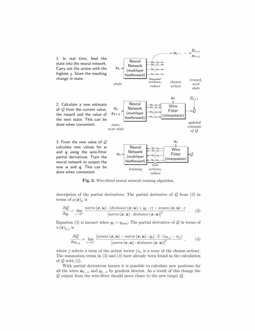
1. In real time, feed thestate into the neural network.Carry out the action with thehighest q. Store the resultingchange in state.

utRt+1

xt+1

xt //

NeuralNetwork

(multilayerfeedforward)

u0,q0 //u1,q1 //uk,qk //

//

un,qn //

......

//___

state actions,values

︸ ︷︷ ︸chosenaction

reward,nextstate

2. Calculate a new estimateof Q from the current value,the reward and the value ofthe next state. This can bedone when convenient.

ut Rt+1

��xt

xt+1

//

NeuralNetwork

(multilayerfeedforward)

u0,q0 //u1,q1 //uk,qk //un,qn //

WireFitter

(interpolator)

//Q......

��

state,next state

updatedestimate

of Q

3. From the new value of Qcalculate new values for uand q using the wire-fitterpartial derivatives. Train theneural network to output thenew u and q. This can bedone when convenient.

ut

xt //

NeuralNetwork

(multilayerfeedforward)

oo u0,q0oo u1,q1

oo uk,qk

oo un,qn

WireFitter

(interpolator)

oo Q......

��

trainingnew

actions,values

︸ ︷︷ ︸Fig. 3. Wire-fitted neural network training algorithm.

description of the partial derivatives. The partial derivative of Q from (2) interms of q (x)k is

∂Q∂qk

= limε→0+

norm (x,u) · (distance (x,u) + qk · c)− wsum (x,u) · c[norm (x,u) · distance (x,u)]2

. (3)

Equation (3) is inexact when qk = qmax. The partial derivative of Q in terms ofu (x)k,j is

∂Q∂uk,j

= limε→0+

[wsum (x,u)− norm (x,u) · qk] · 2 · (uk,j − uj)[norm (x,u) · distance (x,u)]2

, (4)

where j selects a term of the action vector (uj is a term of the chosen action).The summation terms in (3) and (4) have already been found in the calculationof Q with (2).

With partial derivatives known it is possible to calculate new positions forall the wires u0...n and q0...n by gradient descent. As a result of this change theQ output from the wire-fitter should move closer to the new target Q.

6 Practical Issues

When the input to a neural network changes slowly a problem known as unlearn-ing or interference can cause the network to unlearn the correct output for otherinputs because recent experience dominates the training data [16]. We cope withthis problem by storing examples of state, action and next state transitions andreplaying them as if they are being re-experienced. This creates a constantlychanging input to the neural network, known as a persistent excitation. We donot store target outputs for the network as these would become incorrect throughthe learning process described in Sect. 5. Instead the wire-fitter is used to cal-culate new neural network output targets. This method makes efficient use ofdata gathered from the world without relying on extrapolation. A disadvantageis that if conditions change the stored data could become misleading.

One problem with applyingQ-learning to continuous problems is that a singlesuboptimal action will not prevent a high value action from being carried out atthe next time step. Thus the value of actions in a particular state can be verysimilar, as the value of the action in the next time step will be carried back. Asthe Q-value is only approximated for continuous states and actions it is likelythat most of the approximation power will be used representing the values of thestates rather than actions in states. The relative values of actions will be poorlyrepresented, resulting in an unsatisfactory policy. The problem is compoundedas the time intervals between control actions get smaller.

Advantage Learning [4] addresses this problem by emphasising the differencesin value between the actions. In Advantage Learning the value of the optimalaction is the same as for Q-learning, but the lesser value of non-optimal actionsis emphasised by a scaling factor (k ∝ ∆t). This makes a more efficient use ofthe approximation resources available. The Advantage Learning update is

A (x,u) := (1− α)A (x,u)

+ α[

1k

(R+ γk maxA (xt+1,ut+1)

)+(1− 1

k

)maxA (xt,ut)

], (5)

where A is analogous to Q in (1). The results in Sect. 7 show that AdvantageLearning does make a difference in our learning task.

7 Simulation Results

We apply our learning algorithm to a simulation task. The task involves guiding asubmersible vehicle to a target position by firing thrusters located on either side.The thrusters produce continuously variable thrust ranging from full forward tofull backward. As there are only two thrusters (left, right) but three degrees onfreedom (x, y, rotation) the submersible is non-holonomic in its planar world.The simulation includes momentum and friction effects in both angular andlinear displacement. The controller must learn to slow the submersible and holdposition as it reaches the target. Reward is the negative of the distance to thetarget (this is not a pure delayed reward problem).

Fig. 4. Appearance of the simulator for one run. The submersible gradually learns tocontrol its motion to reach targets

Figure 4 shows a simulation run with hand placed targets. At the pointmarked zero the learning system does not have any knowledge of the effects ofits actuators, the meaning of its sensors, or even the task to be achieved. Aftersome initial wandering the controller gradually learns to guide the submersibledirectly toward the target and come to a near stop.

In earlier results using Q-learning alone [17], the controller learned to directthe submersible to the first randomly placed target about 70% of the time. Lessthan half of the controllers could reach all in series of 10 targets. Observation ofQ-values showed that the value varied only slightly between actions, making itdifficult to learn a stable policy. In our current implementation we use AdvantageLearning (see Sect. 6) to emphasise the differences between actions. We nowreport that 100% of the controllers converge to acceptable performance.

To test this, we placed random targets at a distance of 1 unit, in a randomdirection, from a simulated submersible robot and allowed a period of 200 timesteps for it to approach and hold station on the target. For a series of targets, theaverage distance over the time period, was recorded. A random motion achievesan average distance of 1 unit (no progress) while a hand coded controller canachieve 0.25. The learning algorithm reduces the average distance with time,eventually approaching hand coded controller performance. Recording distancerather than just ability to reach the target ensures that controllers which fail tohold station don’t receive a high rating.

Graphs comparing 140 controllers trained with Q-learning and 140 trainedwith Advantage Learning are shown in the box-and-whisker plots in Fig. 5. Themedian distance to the target is the horizontal line in the middle of the box. Theupper and lower bounds of the box show where 25% of the data above and below

5 10 15 20 25 30 35 400

0.2

0.4

0.6

0.8

1

1.2

1.4

1.6

1.8

2

Ave

rage

Dis

tanc

e T

o T

arge

t

Target Number5 10 15 20 25 30 35 40

0

0.2

0.4

0.6

0.8

1

1.2

1.4

1.6

1.8

2

Ave

rage

Dis

tanc

e T

o T

arge

t

Target Number

Fig. 5. Performance of 140 learning controllers using Q-learning (left) and AdvantageLearning (right) which attempt to reach 40 targets each placed one distance unit away

the median lie, so the box contains the middle 50% of the data. Outliers, whichare outside 1.5 times the range between the upper and lower ends of the boxfrom the median, are shown by a “+” sign. The whiskers show the range of thedata, excluding outliers. Advantage Learning converges to good performancemore quickly and reliably than Q-learning and with many fewer and smallermagnitude spurious actions. Gradual improvement is still taking place at the40th target. The quantity of outliers on the graph for Q-learning show that thepolicy continues to produce erratic behaviour in about 10% of cases.

When reward is based only on distance to the target (as in the experimentabove) the actions are somewhat step like. To promote smooth control it isnecessary to punish for both energy use and sudden changes in commandedaction. Such penalties encouraged smoothness and confirmed that the system iscapable of responding to continuous changes in state with continuous changes inaction. A side effect of punishing for consuming energy is an improved ability tomaintain position.

8 Conclusion

A practical continuous state, continuous action Q-learning system has been de-scribed and tested. It was found to converge quickly and reliably on a simulatedcontrol task. Advantage Learning was found to be an important tool in over-coming the problem of similarity in value between actions.

Acknowledgements

We thank WindRiver Systems and BEI Systron Donner for their support ofthe Kambara AUV project. We also thank the Underwater Robotics projectteam: Samer Abdallah, Terence Betlehem, Wayne Dunston, Ian Fitzgerald, ChrisMcPherson, Chanop Silpa-Anan and Harley Truong for their contributions.

References

[1] Richard S. Sutton and Andrew G. Barto. Reinforcement Learning: An Introduc-tion. Bradford Books, MIT, 1998.

[2] Christopher J. C. H. Watkins. Learning from Delayed Rewards. PhD thesis,University of Cambridge, 1989.

[3] A. G. Barto, R. S. Sutton, and C. W. Anderson. Neuronlike adaptive elementsthat can solve difficult learning control problems. IEEE Trans on systems, manand cybernetics, SMC-13:834–846, 1983.

[4] Mance E. Harmon and Leemon C. Baird. Residual advantage learning appliedto a differential game. In Proceedings of the International Conference on NeuralNetworks, Washington D.C, 1995.

[5] Paul J. Werbos. Approximate dynamic programming for real-time control andneural modeling. In D. A. White and D. A. Sofge, editors, Handbook of IntelligentControl: Neural, Fuzzy, and Adaptive Approaches. Van Nostrand Reinhold, 1992.

[6] Juan C. Santamaria, Richard S. Sutton, and Ashwin Ram. Experiments with rein-forcement learning in problems with continuous state and action spaces. AdaptiveBehaviour, 6(2):163–218, 1998.

[7] Gavin Adrian Rummery. Problem solving with reinforcement learning. PhD thesis,Cambridge University, 1995.

[8] Claude F. Touzet. Neural reinforcement learning for behaviour synthesis. Roboticsand Autonomous Systems, 22(3-4):251–81, 1997.

[9] H.-M. Gross, V. Stephan, and M. Krabbes. A neural field approach to topo-logical reinforcement learning in continuous action spaces. In Proc. 1998 IEEEWorld Congress on Computational Intelligence, WCCI’98 and International JointConference on Neural Networks, IJCNN’98, Anchorage, Alaska, 1998.

[10] J. S. Albus. A new approach to manipulator control: the cerebrellar model ar-ticulated controller (CMAC). J. Dynamic Systems, Measurement and Control,97:220–227, 1975.

[11] Long-Ji Lin. Self-improving reactive agents based on reinforcement learning, plan-ning and teaching. Machine Learning Journal, 8(3/4), 1992.

[12] T. Kohonen. Self-Organization and Associative Memory. Springer, Berlin, thirdedition, 1989.

[13] Juan Miguel Santos. Contribution to the study and design of reinforcement func-tions. PhD thesis, Universidad de Buenos Aires, Universite d’Aix-Marseille III,1999.

[14] Leemon C. Baird and A. Harry Klopf. Reinforcement learning with high-dimensional, continuous actions. Technical Report WL-TR-93-1147, Wright Lab-oratory, 1993.

[15] Peter Lancaster and Kestutis Salkauskas. Curve and Surface Fitting, an Intro-duction. Academic Press, 1986.

[16] W. Baker and J. Farrel. An introduction to connectionist learning control systems.In D. A. White and D. A. Sofge, editors, Handbook of Intelligent Control: Neural,Fuzzy, and Adaptive Approaches. Van Nostrand Reinhold, 1992.

[17] Chris Gaskett, David Wettergreen, and Alexander Zelinsky. Reinforcement learn-ing applied to the control of an autonomous underwater vehicle. In Proceedingsof the Australian Conference on Robotics and Automation (AuCRA99), 1999.