Sandia is a multiprogram laboratory operated by Sandia Corporation, a Lockheed Martin Company,for the United States Department of Energy’s National Nuclear Security Administration

under contract DE-AC04-94AL85000.

Pyomo: Python Optimization Modeling Objects

William E. HartSandia National Laboratories

wehart@sandia.gov

Slide 2

Pyomo

Idea: support mathematical modeling of integer programs in Python

– Support for MINLP is a longer-term goal

Why Math Modeling?

– Provide a natural syntax to describe mathematical models– Can formulate large models with a concise syntax– Separate modeling and data declarations– Support sophisticated data indexing to facilitate modeling with

structured data– Support data import and export in commonly used formats– Include tools for debugging a model

Examples: AMPL, GAMS, OptimJ, AIMMS, FlopCPP, …

Slide 3

Requirements

Open Source– Transparency and reliability– Customizable capability– Flexible licensing

Flexible Modeling Language– Extensibility and robustness– Documentation– Standard libraries– Support for standard programming language features

• Classes, functionsPortability

– Linux, MS Windows, Mac OSSolver Integration

– Tight integration: solvers linked into modeling language– Loose integration: solver launched separately

Abstract Models– Symbolic representation of objectives and constraints

Slide 4

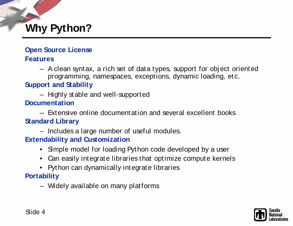
Why Python?

Open Source LicenseFeatures

– A clean syntax, a rich set of data types, support for object oriented programming, namespaces, exceptions, dynamic loading, etc.

Support and Stability– Highly stable and well-supported

Documentation– Extensive online documentation and several excellent books

Standard Library– Includes a large number of useful modules.

Extendability and Customization• Simple model for loading Python code developed by a user• Can easily integrate libraries that optimize compute kernels• Python can dynamically integrate libraries

Portability– Widely available on many platforms

Slide 5

Other Programming Languages

.Net

– Only available on MS WindowsRuby

– A widely used scripting language with strong support– More complicated syntax than Python

C++

– Requires explicit compilation– No interactive interpreter

Java

– Meets most of the requirements outlined previously– No interactive interpreter (?)– Python’s dynamic typing and concise syntax makes software

development quick and easy

Slide 6

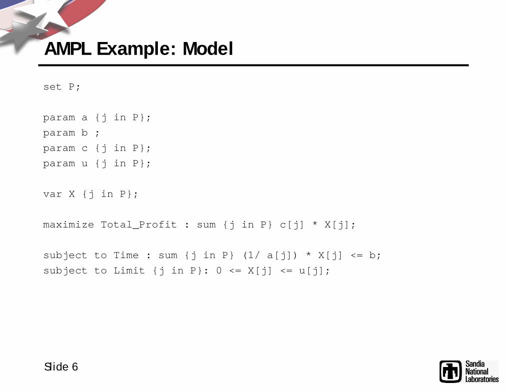
AMPL Example: Model

set P;

param a {j in P};

param b ;

param c {j in P};

param u {j in P};

var X {j in P};

maximize Total_Profit : sum {j in P} c[j] * X[j];

subject to Time : sum {j in P} (1/ a[j]) * X[j] <= b;

subject to Limit {j in P}: 0 <= X[j] <= u[j];

Slide 7

AMPL Example: Data

data;

set P := bands coils;

param: a c u :=

bands 200 25 6000

coils 140 30 4000 ;

param b := 40;

Slide 8

Pyomo Example: Model (1)

#

# Coopr import

#

from coopr.pyomo import *#

# Setup the model

#

model = Model()

#

# Declare sets, parameters and variables

#

model.P = Set()

model.a = Param(model.P)

model.b = Param()

model.c = Param(model.P)

model.u = Param(model.P)

model.X = Var(model.P)

Slide 9

Pyomo Example: Model (2)

#

# Declare objective rule and create objective object

#

def Objective_rule(model):

ans = 0

for j in model.P:

ans = ans + model.c[j] * model.X[j]

return ans

model.Total_Profit = Objective(rule=Objective_rule,

sense=maximize)

Slide 10

Pyomo Example: Model (3)

## Declare constraint rules and create objective objects## Time#def Time_rule(model):ans = 0for j in model.P:

ans = ans + (model.X[j]/model.a[j])return ans < model.b

model.Time = Constraint(rule=Time_rule)## Limit#def Limit_rule(j, model):return(0, model.X[j], model.u[j])

model.Limit = Constraint(model.P, rule=Limit_rule)

Slide 11

AMPL Example: Solving Model

% ampl

ampl: model prod.mod;

ampl: data prod.dat;

option solver PICO;

solve;

No integer variables... solving the LP normally.

LP value= 192000

CPU RunTime= 0

CPU TotalTime= 0.109

WallClock TotalTime= 0.109375

PICO Solver: final f = 192000.000000

Slide 12

Pyomo Example: Solving Model (1)

% pyomo prod.py prod.dat

==========================================================--- Solver Results ---==========================================================---------------------------------------------------------------- Problem Information ----------------------------------------------------------------name: Nonenum_constraints: 5num_nonzeros: 6num_objectives: 1num_variables: 2sense: maximizeupper_bound: 192000

Slide 13

Pyomo Example: Solving Model (2)

---------------------------------------------------------------- Solver Information ----------------------------------------------------------------error_rc: 0nbounded: Nonencreated: Nonestatus: oksystime: Noneusrtime: None

---------------------------------------------------------------- Solution 0----------------------------------------------------------gap: 0.0status: optimalvalue: 192000Primal Variables

X_bands_ 6000X_coils_ 1400

Dual Variablesc_u_Limit_1 4c_u_Time_0 4200

----------------------------------------------------------

Slide 14

Solving a Pyomo Model within Python

#

# Imports

import prod

from coopr.pyomo import *

#

# Configure Coopr

coopr.opt.config().configure()

#

# Create the model instance

instance = prod.model.create("prod.dat")

#

# Setup the optimizer

opt = solvers.SolverFactory("glpk")

#

# Optimize

results = opt.solve(instance)

#

# Write the output

results.write(num=1)

Slide 15

AMPL/Pyomo Comparison

• Pyomo object/constraint declarations are more verbose– Typically requires the use of a temporary function

• Pyomo declarations explicitly refer to models– Can declare multiple models and model instances

• Pyomo can apply solvers that do not recognize the *.nl format

• Pyomo (currently) only supports linear models– Linear programs and mixed-integer linear programs

• Pyomo does not include preprocessing of LP/MILP instances

• Pyomo can work with a richer programming environment

Slide 16

Customizing Pyomo

• Adding diagnostic information during generation

• Generation of model instance (using custom generation method)

• Custom set/parameter definitions

• Data integration with external data sources

– Databases, spreadsheets, Python classes, etc…

Note: the default generation process is sufficient for current Pyomo applications

Slide 17

Related Python Optimization Tools

Python Optimizer Packages

– CVXOPT– SciPy– OpenOpt– NLPy– Pyipopt

Python Optimization Modeling Packages

– PuLP• Direct construction of LP/MILP models

– POAMS• Symbolic representation of LP/MILP models

Slide 18

Coordinating with POAMS and PuLP

• Integration of Pyomo, POAMS and PuLP capabilities?– Tight integration may not happen

• Developers have different design requirements and/or research goals

– Idea: share common components and/or core infrastructure

• Plugin support for extensibility– Registration of optimizers– Registration of modeling tools

Example: preprocessing– Broadly applicable to LP & MILP models– Idea: leverage common ‘instance’ representation– Idea: leverage plugins to customize preprocessing

• Standard techniques• Application-specific techniques

– Challenge: map preprocessing changes into original model representations

Slide 19

Pyomo and Coopr

Pyomo is a Python package that is managed within the Coopr software.

Coopr:– COmmon Optimization Python Repository– Integrates a variety of optimization-related Python packages– Designed to support the Acro software project

Coopr Opt– Commonly-used optimization utilities

• Solver results• Problem transformations

– Optimization solvers• Wrappers to external solvers• Python optimizers

Slide 20

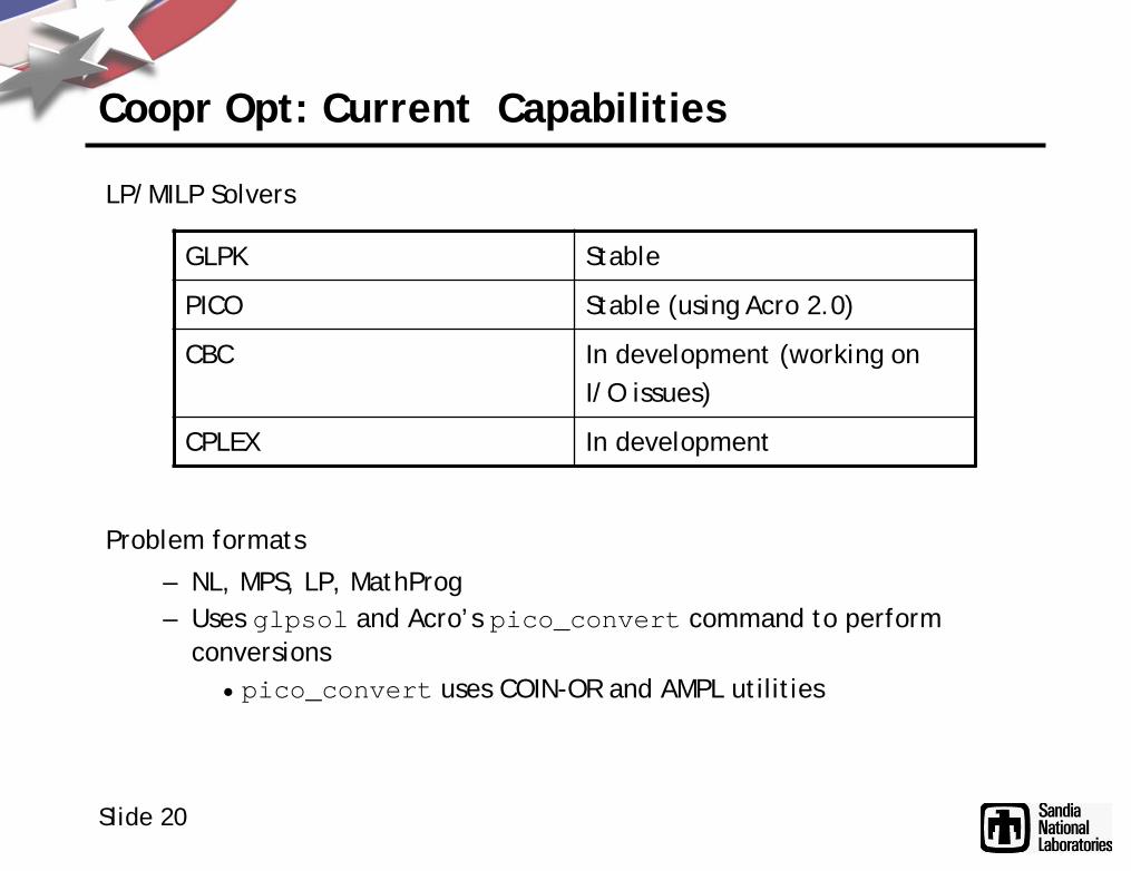
Coopr Opt: Current Capabilities

LP/MILP Solvers

Problem formats

– NL, MPS, LP, MathProg– Uses glpsol and Acro’s pico_convert command to perform

conversions• pico_convert uses COIN-OR and AMPL utilities

GLPK Stable

PICO Stable (using Acro 2.0)

CBC In development (working on I/O issues)

CPLEX In development

Slide 21

Future Directions

• Extensible plugin architecture

• Support for nonlinear models

– Possible integration with SAGE to support AD

• Interfacing with Python optimization packages

– E.g. interface with SciPy, OpenOpt, etc

• Solver interfaces

– Direct solver interfaces– Support for the COIN-OR OS services

• Distributions

– Windows installers– PyPi support (to enable use of the Python easy_install utility)

Slide 22

Related Talks

• Acro 2.0: A Common Respository for Optimizers– MB05

• Object-algebraic Modeling Using POAMS: Meta-algorithms– TA05

• SUCASA, Implementing a Facility for Exposing Mathematical Programming Language Names in Customized Integer Programming Codes

– TB04

• Using SUCASA, Developing Integer Programming Solver Customizations Using Natural Names

– TB04

Slide 23

Getting Started

Coopr 1.0 release has been recently finalized

Downloads:

https://software.sandia.gov/trac/coopr/downloader

Online Documentation

https://software.sandia.gov/trac/coopr/wiki/Package/Pyomo