
PURIFY: a new approach to radio-interferometric imaging · PURIFY: a new approach to...
14
Mon. Not. R. Astron. Soc. 000, 1–14 (2014) Printed February 5, 2014 (MN L A T E X style file v2.2) PURIFY: a new approach to radio-interferometric imaging R. E. Carrillo 1? , J. D. McEwen 2,3 and Y. Wiaux 1,4,5,6 1 Institute of Electrical Engineering, Ecole Polytechnique F´ ed´ erale de Lausanne (EPFL), CH-1015 Lausanne, Switzerland 2 Department of Physics and Astronomy, University College London (UCL), London WC1E 6BT, UK 3 Mullard Space Science Laboratory, University College London (UCL), Holmbury St Mary, Surrey RH5 6NT, UK 4 Department of Medical Radiology, University Hospital Center (CHUV) and University of Lausanne (UNIL), CH-1011 Lausanne, Switzerland 5 Department of Radiology and Medical Informatics, University of Geneva (UniGE), CH-1211 Geneva, Switzerland 6 Institute of Sensors, Signals & Systems, Heriot-Watt University, Edinburgh EH14 4AS, UK Accepted —. Received —; in original form — ABSTRACT In a recent article series, the authors have promoted convex optimization algorithms for radio-interferometric imaging in the framework of compressed sensing, which leverages sparsity regularization priors for the associated inverse problem and defines a minimiza- tion problem for image reconstruction. This approach was shown, in theory and through simulations in a simple discrete visibility setting, to have the potential to outperform sig- nificantly CLEAN and its evolutions. In this work, we leverage the versatility of convex optimization in solving minimization problems to both handle realistic continuous visibil- ities and offer a highly parallelizable structure paving the way to significant acceleration of the reconstruction and high-dimensional data scalability. The new algorithmic structure promoted relies on the simultaneous-direction method of multipliers (SDMM), and contrasts with the current major-minor cycle structure of CLEAN and its evolutions, which in par- ticular cannot handle the state-of-the-art minimization problems under consideration where neither the regularization term nor the data term are differentiable functions. We release a beta version of an SDMM-based imaging software written in C and dubbed PURIFY (http://basp-group.github.io/purify/) that handles various sparsity priors, in- cluding our recent average sparsity approach SARA. We evaluate the performance of different priors through simulations in the continuous visibility setting, confirming the superiority of SARA. Key words: techniques: image processing – techniques: interferometric. 1 INTRODUCTION Radio interferometry is a powerful technique that allows observa- tion of the radio emission from the sky with high angular resolution and sensitivity, providing valuable information for astrophysics, as- trometry and cosmology (Ryle & Vonberg 1946; Blythe 1957; Ryle et al. 1959; Ryle & Hewish 1960; Thompson et al. 2001). The mea- surement equation for radio interferometry defines an ill-posed lin- ear inverse problem in the perspective of signal reconstruction. Un- der restrictive assumptions of monochromatic non-polarized imag- ing on small fields of view (FOV), the measured visibilities relates to Fourier measurements of the observed signal. Next-generation radio telescopes, such as the new LOw Frequency ARray (LO- FAR 1 ), or the recently upgraded Karl G. Jansky Very Large Ar- ray (VLA 2 ), or the future Square Kilometer Array (SKA 3 ), will ? E-mail: rafael.carrillo@epfl.ch 1 http://www.lofar.org/ 2 https://science.nrao.edu/facilities/vla 3 http://www.skatelescope.org/ achieve much higher dynamic range than current instruments, also at higher angular resolution. Also, these telescopes will acquire a massive amount of data, thus posing large-scale problems. Classi- cal imaging techniques developed in the field, such as the CLEAN algorithm and its multi-scale variants (H¨ ogbom 1974; Bhatnagar & Cornwell 2004; Cornwell 2008), are known to be slow and to provide suboptimal imaging quality (Li et al. 2011; Carrillo et al. 2012). This state of things has triggered an intense research to re- formulate imaging techniques for radio interferometry in the per- spective of next-generation instruments. The theory of compressed sensing (CS) introduces a signal acquisition and reconstruction framework that goes beyond the tra- ditional Nyquist sampling paradigm (Donoho 2006; Cand` es 2006; Baraniuk 2007; Fornasier & Rauhut 2011). Recently, CS and con- vex optimization techniques have been applied to image deconvo- lution in radio interferometry (Wiaux et al. 2009a,b; Wenger et al. 2010; McEwen & Wiaux 2011; Li et al. 2011; Carrillo et al. 2012) showing promising results. These techniques promise improved image fidelity, flexibility and computation speed over traditional c 2014 RAS
Transcript of PURIFY: a new approach to radio-interferometric imaging · PURIFY: a new approach to...

Mon Not R Astron Soc 000 1ndash14 (2014) Printed February 5 2014 (MN LATEX style file v22)
PURIFY a new approach to radio-interferometric imaging
R E Carrillo1 J D McEwen23 and Y Wiaux14561Institute of Electrical Engineering Ecole Polytechnique Federale de Lausanne (EPFL) CH-1015 Lausanne Switzerland2Department of Physics and Astronomy University College London (UCL) London WC1E 6BT UK3Mullard Space Science Laboratory University College London (UCL) Holmbury St Mary Surrey RH5 6NT UK4Department of Medical Radiology University Hospital Center (CHUV) and University of Lausanne (UNIL) CH-1011 Lausanne Switzerland5Department of Radiology and Medical Informatics University of Geneva (UniGE) CH-1211 Geneva Switzerland6Institute of Sensors Signals amp Systems Heriot-Watt University Edinburgh EH14 4AS UK
Accepted mdash Received mdash in original form mdash
ABSTRACTIn a recent article series the authors have promoted convex optimization algorithms forradio-interferometric imaging in the framework of compressed sensing which leveragessparsity regularization priors for the associated inverse problem and defines a minimiza-tion problem for image reconstruction This approach was shown in theory and throughsimulations in a simple discrete visibility setting to have the potential to outperform sig-nificantly CLEAN and its evolutions In this work we leverage the versatility of convexoptimization in solving minimization problems to both handle realistic continuous visibil-ities and offer a highly parallelizable structure paving the way to significant accelerationof the reconstruction and high-dimensional data scalability The new algorithmic structurepromoted relies on the simultaneous-direction method of multipliers (SDMM) and contrastswith the current major-minor cycle structure of CLEAN and its evolutions which in par-ticular cannot handle the state-of-the-art minimization problems under consideration whereneither the regularization term nor the data term are differentiable functions We releasea beta version of an SDMM-based imaging software written in C and dubbed PURIFY(httpbasp-groupgithubiopurify) that handles various sparsity priors in-cluding our recent average sparsity approach SARA We evaluate the performance of differentpriors through simulations in the continuous visibility setting confirming the superiority ofSARA
Key words techniques image processing ndash techniques interferometric
1 INTRODUCTION
Radio interferometry is a powerful technique that allows observa-tion of the radio emission from the sky with high angular resolutionand sensitivity providing valuable information for astrophysics as-trometry and cosmology (Ryle amp Vonberg 1946 Blythe 1957 Ryleet al 1959 Ryle amp Hewish 1960 Thompson et al 2001) The mea-surement equation for radio interferometry defines an ill-posed lin-ear inverse problem in the perspective of signal reconstruction Un-der restrictive assumptions of monochromatic non-polarized imag-ing on small fields of view (FOV) the measured visibilities relatesto Fourier measurements of the observed signal Next-generationradio telescopes such as the new LOw Frequency ARray (LO-FAR1) or the recently upgraded Karl G Jansky Very Large Ar-ray (VLA2) or the future Square Kilometer Array (SKA3) will
E-mail rafaelcarrilloepflch1 httpwwwlofarorg2 httpssciencenraoedufacilitiesvla3 httpwwwskatelescopeorg
achieve much higher dynamic range than current instruments alsoat higher angular resolution Also these telescopes will acquire amassive amount of data thus posing large-scale problems Classi-cal imaging techniques developed in the field such as the CLEANalgorithm and its multi-scale variants (Hogbom 1974 Bhatnagaramp Cornwell 2004 Cornwell 2008) are known to be slow and toprovide suboptimal imaging quality (Li et al 2011 Carrillo et al2012) This state of things has triggered an intense research to re-formulate imaging techniques for radio interferometry in the per-spective of next-generation instruments
The theory of compressed sensing (CS) introduces a signalacquisition and reconstruction framework that goes beyond the tra-ditional Nyquist sampling paradigm (Donoho 2006 Candes 2006Baraniuk 2007 Fornasier amp Rauhut 2011) Recently CS and con-vex optimization techniques have been applied to image deconvo-lution in radio interferometry (Wiaux et al 2009ab Wenger et al2010 McEwen amp Wiaux 2011 Li et al 2011 Carrillo et al 2012)showing promising results These techniques promise improvedimage fidelity flexibility and computation speed over traditional
ccopy 2014 RAS
2 Carrillo et al
approaches This speed enhancement is crucial for the scalabilityof imaging techniques to very high dimensions in the perspectiveof next-generation telescopes However CS-based imaging tech-niques have only been studied for low dimensional discrete visibil-ity coverages The works in Wiaux et al (2009ab) and McEwenamp Wiaux (2011) consider idealised random and discrete visibilitycoverages in order to remain as close to the CS theory as possibleFirst steps towards more realistic visibility coverages have beentaken by Wenger et al (2010) and Li et al (2011) who considercoverages due to specific interferometer configurations but whichremain discrete Carrillo et al (2012) consider variable densitysampling patterns which mimic common generic sampling pat-terns in radio-interferometric (RI) imaging but also remaining dis-crete These preliminary works suggest that the performance of CSreconstructions is likely to hold for more realistic visibility cover-ages Therefore the extension of CS techniques to more realisticcontinuous interferometric measurements is of great importance
In the present work we extend the previously proposed imag-ing approaches in Wiaux et al (2009a) Wiaux et al (2009b)and Carrillo et al (2012) to handle continuous visibilities andopen the door to large-scale optimization problems We pro-pose a general algorithmic framework based on the simultaneous-direction method of multipliers (SDMM) to solve sparse imagingproblems The proposed framework offers a parallel implemen-tation structure that decomposes the original problem into severalsmall simple problems hence allowing implementation in mul-ticore architectures or in computer clusters or on graphics pro-cessing units These implementations provide both flexibility inmemory requirements and a significant gain in terms of speedthus enabling scalability to large-scale problems SDMM standsin stark contrast with the current major-minor cycle structure ofCLEAN and evolutions which in particular cannot handle thestate-of-the-art minimization problems under consideration (Car-rillo et al 2012) where neither the regularization term nor the dataterm are differentiable functions We release a beta version of anSDMM-based imaging software written in C and dubbed PURIFY(httpbasp-groupgithubiopurify) that handlesvarious sparsity priors including our recent average sparsity ap-proach SARA (Carrillo et al 2012) thus providing a new powerfulframework for RI imaging We evaluate the performance of differ-ent priors through simulations in the continuous visibility settingSimulation results confirm the superiority of SARA for continuousFourier measurements Even though this beta version of PURIFYis not parallelized we discuss in detail the extraordinary paralleland distributed optimization potential of SDMM to be exploited infuture versions
The remainder of the paper is organized as follows In Sec-tion 2 we review the theory of CS briefly In Section 3 we recallthe inverse problem for image reconstruction from RI data and de-scribe the state-of-the-art image reconstruction techniques used inradio astronomy Section 4 presents the SDMM-based algorithmfor RI imaging which enables the incorporation of any convexsparsity regularization prior In Section 5 we describe the PURIFYpackage including implementation details Numerical results eval-uating the different regularization priors included in PURIFY inparticular SARA are presented in Section 6 Finally we concludein Section 7
2 COMPRESSED SENSING
CS introduces a signal acquisition framework that goes beyondthe traditional Nyquist sampling paradigm (Donoho 2006 Candes2006 Baraniuk 2007 Fornasier amp Rauhut 2011) demonstratingthat sparse signals may be recovered accurately from incompletedata Consider a complex-valued signal x isin CN assumed tobe sparse in some orthonormal basis Ψ isin CNtimesN with K Nnonzero coefficients and also consider the measurement modely = Φx + n where y isin CM denotes the measurement vectorΦ isin CMtimesN is the sensing matrix and n isin CM represents the ob-servation noise The standard condition M lt N characterizes theincompleteness of the data The most common approach to recoverx from y is to solve the following convex problem (Fornasier ampRauhut 2011)
minαisinCN
α1 subject to y minus ΦΨα2 6 ε (1)
where ε is an upper bound on the `2 norm of the noise and middot 1denotes the `1 norm of a complex-valued vector The signal is re-covered as x = Ψα where α denotes the solution to the aboveproblem Such problems that solve for the representation of thesignal in a sparsity basis are known as synthesis-based problems
The standard theory of CS provides results for the recoveryof x from y if Φ obeys a Restricted Isometry Property (RIP) (For-nasier amp Rauhut 2011) A sufficient condition is that M is largerthan roughly the signal sparsity M gt 2K N Note that in-complete Fourier measurements on discrete or continuous spatialfrequencies represent a good sampling approach in this contextIn the continuous setting the theory applies also for M gt N It is not strictly ldquocompressedrdquo sensing any more but the inverseproblem remains ill-posed The basic theory also requires Ψ to beorthonormal However signals often exhibit better sparsity in anovercomplete dictionary (Gribonval amp Nielsen 2003 Bobin et al2007 Starck et al 2010) Therefore recent works have begun toaddress the case of CS with redundant dictionaries In this settingthe signal x is expressed in terms of a dictionary Ψ isin CNtimesD N lt D as x = Ψα α isin CD Rauhut et al (2008) find condi-tions on the dictionary Ψ such that the compound matrix ΦΨ obeysthe RIP to accurately recover α by solving a synthesis-based prob-lem Note that the problem is now more severely underterminedsince the dimensionality of the unknonw has increased from N toD
As opposed to synthesis-based problems analysis-based prob-lems recover the signal itself solving
minxisinCN
Ψdaggerx1 subject to y minus Φx2 6 ε (2)
where Ψdagger denotes the adjoint operator of Ψ In this paper the super-script dagger is used to denote both operator adjoint or conjugate trans-pose Candes et al (2010) provide a theoretical analysis of the `1analysis-based problem extending the standard CS theory to coher-ent and redundant dictionaries They provide theoretical stabilityguarantees based on a general condition of the sensing matrix Φcoined the Dictionary Restricted Isometry Property (D-RIP) Notethat in the case when redundant dictionaries are used the analysisproblem does not increase the dimensionality of the problem as itsolves for the signal itself Empirical and theoretical studies haveshown clear advantages of the analysis approach over the synthe-sis approach for imaging problems (Carrillo et al 2013) See Namet al (2013) and references therein for further discussion of theanalysis model
ccopy 2014 RAS MNRAS 000 1ndash14
PURIFY 3
3 RADIO-INTERFEROMETRIC IMAGING
31 Interferometric inverse problem
A radio interferometer is an array of spatially separated antennasthat takes measurements of the radio emissions of the sky the so-called visibilities The visibility coordinates are given by the rel-ative position between each pair of antennas The baseline com-ponents (u v w) are measured in units of the wavelength λ of theincoming signal The components u = (u v) specify the planarbaseline coordinates while the third component w is associatedwith the basis vector of the coordinate pointing towards the centerof the FOV of the telescope The sky brightness distribution x canbe described in the same coordinate system as the baseline withcomponents (lm n) where l = (lm) denotes the coordinateson the image plane and n(l) =
radic1minus l2 minusm2 The general RI
equation for monochromatic non-polarized imaging reads as
y (u) =
intA (lu)x (l) eminus2πiumiddotl d2l (3)
whereA (lu) = Aprime (lu)nminus1(l) andAprime (lu) stands for all con-tributions of direction dependent effects (DDE) Examples of DDEsare the primary beam which limits the observed FOV and the w-term eminus2πiw(n(l)minus1) This general equation defines a linear inverseproblem in the perspective of recovering the intensity signal x fromthe measured visibilities (Rau et al 2009) Under the assumptionsof small FOV (n asymp 1) or when the array is coplanar (w asymp 0) eachvisibility corresponds to the measurement of the Fourier transformof a planar signal at the spatial frequency u This result is knownas the van Cittert-Zernike theorem (Thompson et al 2001) Thetotal number of points u probed by all telescope pairs of the arrayduring the observation provides some incomplete coverage in theFourier plane the so-called u-v coverage characterizing the inter-ferometer
To recover the source image from incomplete visibility mea-surements we pose the inverse problem (3) for a sampled version ofthe image The band-limited functions considered are completelyidentified by their Nyquist-Shannon sampling on a discrete uniformgrid ofN = N12timesN12 points in real space The sampled inten-sity signal is denoted by the vector x isin RN We takeM visibilitiesdenoted by the vector y isin CM which are related to the discreteimage by the following linear model
y = Φx+ n (4)
where Φ isin CMtimesN represents the general linear map from the im-age space domain to the visibility domain which defines an ill-posed inverse problem in the perspective of image reconstructionIn the particular case when the visibilities identify with Fouriersamples the measurement essentially reduces to a Fourier matrixsampled on M spatial frequencies (see eq (31) in Section 5) Ina realistic continuous visibility setting one usually has M gt Nand sometimes M N which will be increasingly the case fornext-generation telescopes
32 State-of-the-art of classic imaging algorithms
The most standard image reconstruction algorithm from visibilitymeasurements is called CLEAN which is a non-linear deconvolu-tion method based on local iterative beam removal (Hogbom 1974Schwarz 1978 Thompson et al 2001) A sparsity prior on the orig-inal signal in real space is implicitly introduced thus already takingadvantage of CS theory guarantees Furthermore as discussed inCornwell (2008) and Wiaux et al (2009a) the CLEAN algorithm
and its variants are examples of the Matching Pursuit algorithm(Mallat amp Zhang 1993) which is well known in the CS commu-nity CLEAN can be considered as a steepest descend algorithm tominimize the objective function χ2 = y minus Φx22 subject to animage model regularization (Rau et al 2009) Most variants oper-ate iteratively in two steps called the major and minor cycles Themajor cycle computes the residual image r(t) = Φdagger(y minus Φx(t))which is the gradient of the χ2 objective function at iteration t Theminor cycle regularizes the image update by applying an operatorT which represents a deconvolution of the operator Φ to the resid-ual image yielding updates of the form
x(t+1) = x(t) + T(r(t)) (5)
A multi-scale version of CLEAN MS-CLEAN has also beendeveloped (Cornwell 2008) where the sparsity model is improvedby multi-scale decomposition hence enabling better recovery ofthe signal The MS-CLEAN method was shown to perform betterthan the standard CLEAN but still suffers from an empirical choiceof basis profiles and scales An adaptive scale pixel decomposi-tion method called ASP-CLEAN was also introduced to improveon multi-scale CLEAN by relying on an adaptive choice of scales(Bhatnagar amp Cornwell 2004) ASP-CLEAN models an image asa superposition of atoms in a redundant dictionary parametrized byamplitude location and scale Thus this algorithm can be seenas a Matching Pursuit algorithm with an overcomplete dictionaryNote that these approaches are known to be slow sometimes pro-hibitively so Variants of CLEAN that addresses wide-band effectsor atmospheric effects have also been proposed in the literature (seeRau et al (2009) Bhatnagar et al (2008a) Bhatnagar et al (2013)and references therein)
Another approach to the reconstruction of images from visi-bility measurements is the Maximum Entropy Method (MEM) Incontrast to CLEAN MEM solves a global optimization problem inwhich the inverse problem is regularized by the introduction of anentropic prior on the signal but sparsity is not explicitly required(Cornwell amp Evans 1985) In practice CLEAN and variants havefound more widespread application than MEM
33 State-of-the-art of convex imaging algorithms
Reconstruction techniques based on CS and convex optimizationhave also been proposed The relationship between CLEAN and`1 minimization coupled with a Dirac basis was first studied byMarsh amp Richardson (1987) The first application of CS and con-vex optimization to radio interferometry was performed by Wiauxet al (2009a) where the versatility of the approach and its supe-riority relative to standard interferometric imaging techniques wasdemonstrated It was reported that an `1 minimization problem ofthe form of (1) coupled with a Dirac basis yields similar reconstruc-tion quality to CLEAN while including a positivity constraint in aconvex formulation significantly enhances the reconstruction qual-ity relative to CLEAN The spread spectrum phenomenon associ-ated with the w component on wide FOV observations was shownin Wiaux et al (2009b) to underpin a significant enhancement of theimaging quality independently of the sparsity basis chosen Theseconsiderations pave the way to potential optimization strategies atthe acquisition level in terms of antenna distribution design A CSapproach was developed and evaluated by Wiaux et al (2010) to re-cover the signal induced by cosmic strings in the cosmic microwavebackground McEwen amp Wiaux (2011) generalise the previous CSimaging techniques to a wide FOV recovering interferometric im-ages defined directly on the sphere rather than a tangent plane All
ccopy 2014 RAS MNRAS 000 1ndash14
4 Carrillo et al
of these works consider uniformly random and discrete visibilitycoverage in order to remain as close to the CS theory as possibleWiaux et al (2010) and McEwen amp Wiaux (2011) exploited the factthat many signals in nature are also sparse or compressible in themagnitude of their gradient space in which case the total variation(TV) minimization problem
minxisinCN
xTV subject to y minus Φx2 6 ε (6)
has been shown to yield superior reconstruction results The TVnorm is defined as xTV = nablax1 wherenablax denotes the imagegradient magnitude (Rudin et al 1992)
First steps towards more realistic visibility coverages havebeen taken by Suksmono (2009) and Wenger et al (2010) whoconsider coverages due to specific interferometer configurations butwhich remain discrete The aforementioned works use the follow-ing unconstrained synthesis problem
minαisinCN
1
2y minus ΦΨα22 + λα1 (7)
where λ is a regularization parameter that balances the weight be-tween the fidelity term and the regularization term Wenger et al(2010) reports superior reconstruction quality relative to an auto-matic CLEAN reconstruction and similar results relative to a user-guided CLEAN reconstruction Li et al (2011) studied a CS imag-ing approach based on (7) and the isotropic undecimated wavelettransform reporting results from discrete simulated coverages ofASKAP The reconstruction quality of the isotropic undecimatedwavelet transform method was reported to be superior to those ofCLEAN and MS-CLEAN Minimization of the problem (7) is doneiteratively by a projected gradient algorithm with updates of theform
α(t+1) = Sλ(α(t) + microΨdaggerΦdagger(y minus ΦΨα(t))
) (8)
where Sλ(middot) is the soft-thresholding operator which will be definedin Section 44 This algorithm can be seen as a major-minor cycleupdate where the major cycle computes the gradient of the χ2 datafidelity term and the minor cycle regularizes the solution by apply-ing the soft-thresholding operator
Carrillo et al (2012) proposed an imaging algorithm dubbedsparsity averaging reweighted analysis (SARA) based on aver-age sparsity over multiple bases showing superior reconstructionqualities relative to state-of-the-art imaging methods in the fieldA sparsity dictionary composed of a concatenation of q basesΨ = [Ψ1Ψ2 Ψq] with Ψ isin CNtimesD N lt D is used andaverage sparsity is promoted through the minimization of an analy-sis `0 prior Ψdaggerx0 The concatenation of the Dirac basis and thefirst eight orthonormal Daubechies wavelet bases (Db1-Db8) wasproposed as an effective and simple candidate for a dictionary inthe RI imaging context See Carrillo et al (2013) for further dis-cussions on the average sparsity model the dictionary selection andother applications to compressive imaging
SARA adopts a reweighted `1 minimization scheme to pro-mote average sparsity through the prior Ψdaggerx0 The algorithmreplaces the `0 norm by a weighted `1 norm and solves a sequenceof weighted `1 problems where the weights are essentially the in-verse of the values of the solution of the previous problem (Candeset al 2008) The weighted `1 problem is defined as
minxisinRN
+
WΨdaggerx1 subject to y minus Φx2 6 ε (9)
where W isin RDtimesD denotes the diagonal matrix with positive
weights and RN+ denotes the positive orthant in RN which rep-resents the positivity prior on x Note that problems of the form(6) and (9) involve the minimization of a constrained problem withnon-differentiable functions which rules out smooth optimizationtechniques and do not fit in the major-minor cycle structure ofCLEAN and the projected gradient algorithm Therefore one mustresort to more sophisticated optimization techniques to solve thesenon-smooth problems
4 A LARGE-SCALE OPTIMIZATION ALGORITHM
41 Proximal splitting methods
Convex optimization problems have many attractive properties inparticular the essential property that any local minimum must bea global minimum and thus there exist efficient methods to solvethem Among convex optimization methods proximal splittingmethods offer great flexibility and are shown to capture and ex-tend several well-known algorithms in a unifying framework Ex-amples of proximal splitting algorithms include Douglas-Rachforditerative thresholding projected Landweber projected gradientforward-backward alternating projections alternating directionmethod of multipliers and alternating split Bregman (Combettesamp Pesquet 2011) Proximal splitting methods solve optimizationproblems of the form
minxisinRN
f1(x) + + fS(x) (10)
where f1(x) fS(x) are convex lower semicontinuous func-tions from RN to R not necessarily differentiable Note that anyconvex constrained problem can be formulated as an unconstrainedproblem by using the indicator function of the convex constraintset as one of the functions in (10) ie fk(x) = iC(x) where Crepresents the convex constraint set The indicator function de-fined as iC(x) = 0 if x isin C or iC(x) = +infin otherwise belongsto the class of convex lower semicontinuous functions Also notethat complex-valued vectors are treated as real-valued vectors withtwice the dimension (accounting for real and imaginary parts)
Proximal splitting methods proceed by splitting the contribu-tion of the functions f1(x) fS(x) individually so as to yieldan easily implementable algorithm They are called proximal be-cause each non-smooth function in (10) is incorporated in the min-imization via its proximity operator The proximity operator is anextension of the notion of the set projection operator to more gen-eral functions Let f be a convex lower semicontinuous functionfrom RN to R then the proximity operator of f is defined as
proxf (x) arg minzisinRN
f(z) +1
2xminus z22 (11)
Typically the solution to (10) is reached iteratively by successiveapplication of the proximity operator associated with each functionAn important feature of proximal splitting methods is that they of-fer a powerful framework for solving convex problems in terms ofspeed and scalability of the techniques to very high dimensionsSee Combettes amp Pesquet (2011) for a review of proximal splittingmethods and their applications in signal and image processing
42 Shortcomings of previously used algorithms
The works in Wiaux et al (2009b) McEwen amp Wiaux (2011) andCarrillo et al (2012) solved problems of the form in (9) whereasWenger et al (2010) and Li et al (2011) solved the unconstrained
ccopy 2014 RAS MNRAS 000 1ndash14
PURIFY 5
problem (7) Unconstrained problems are easier to handle and thereexist fast algorithms to solve them such as the FISTA algorithm(Beck amp Teboulle 2009b) However there is no optimal strategyto fix the regularization parameter even if the noise level is knowntherefore constrained problems such as (9) offer a stronger fidelityterm when the noise power is known or can be estimated a prioriHence we focus our attention on solving problem (9) efficientlyWiaux et al (2009b) McEwen amp Wiaux (2011) and Carrillo et al(2012) used a Douglas-Rachford splitting algorithm (Combettes ampPesquet 2007) to solve (9) in a simple discrete setting However ina realistic continuous setting this algorithm presents several short-comings In the following we discuss the main limitations of theDouglas-Rachford algorithm
The Douglas-Rachford splitting algorithm solves the problemby iteratively minimizing the `1 norm and then projecting the resultonto the constraint set Cprime = x isin CN y minus Φx2 6 ε cap RN+until some stopping criteria is achieved The projection onto theset Cprime is a hard optimization problem which in itself requires aniterative algorithm such as the generalized forward-backward al-gorithm This iterative algorithm requires knowledge of the exactoperator norm (maximum singular value) of Φ or at least a closedupper bound to guarantee convergence In the discrete case the ex-act operator norm can be computed and the algorithm achieves afast convergence rate However in the continuous case the oper-ator norm is unknown and its estimation poses a new problem Ifthe estimate of the operator norm is not precise enough the algo-rithm takes many sub-iterations to converge Hence it would beadvantageous to have an algorithm that does not need prior knowl-edge of the operator norm to achieve a fast convergence rate An-other tenet of the Douglas-Rachford algorithm is that it does notoffer a parallel structure which is a desirable property when solv-ing large scale-problems such as those envisaged for the upcomingtelescopes For these reasons we propose to use the simultaneous-direction method of multipliers (SDMM) (Combettes amp Pesquet2011) which is also tailored to solve problems of the form of(10) and circumvents the shortcomings of a Douglas-Rachford ap-proach
43 Simultaneous Direction Method of Multipliers (SDMM)
SDMM has two important properties (i) it does not require dif-ferentiability of any of the functions and (ii) it offers a parallelimplementation structure where all the proximity operators can becomputed in parallel rather than sequentially (Combettes amp Pes-quet 2011) Such a parallel structure is useful when implementingthe algorithms on multicore architectures or on graphics process-ing units thus providing a significant gain in terms of speed andscalability to large-scale problems SDMM is a generalization ofthe alternating-direction method of multipliers (Boyd et al 2010)to a sum of more than two functions As such SDMM uses aug-mented Lagrangian techniques and duality arguments in its deriva-tion In the following we highlight the main steps in the derivationof SDMM tailored to solve (9)
First observe that the problem in (9) can be reformulated asin (10) in the following way
minxisinCN
f1(L1x) + f2(L2x) + f3(L3x) (12)
where L1 = Ψdagger isin CDtimesN L2 = Φ isin CMtimesN and L3 =I isin RNtimesN is the identity matrix In this formulation f1(r1) =Wr11 for r1 isin CD f2(r2) = iB(r2) with B = r2 isin CM y minus r22 6 ε and f3(r3) = iC(r3) with C = RN+ This
problem is also equivalent to solving
minxisinCN r1isinCD
r2isinCM r3isinCN
f1(r1) + f2(r2) + f3(r3) (13)
subject to Lix = ri for i = 1 2 3
The augmented Lagrangian associated with (13) is the saddle func-tion
Lγ(xr1 r2 r3z1z2z3) = (14)3sumi=1
fi(ri) +1
γzdaggeri (Lixminus ri) +
1
2γLixminus ri22
where γ gt 0 is a so-called penalty parameter and z1 isin CD z2 isin CM and z3 isin CN are the dual variables or the Langrangemultipliers SDMM is a primal dual algorithm that proceeds itera-tively by first minimizing Lγ with respect to the primal variablesx r1 r2 r3 and as second step solving the dual problem
maxz1isinCDz2isinCM z3isinCN
J (z1z2z3) (15)
where
J (z1z2z3) = minxisinCN r1isinCD
r2isinCM r3isinCN
Lγ(x r1 r2 r3z1z2z3)
(16)is the dual function The main difference between SDMM andother primal-dual algorithms is that the optimization with respectto the primal variables is done in an alternating fashion by firstminimizing Lγ with respect to x and then with respect to r1 r2r3 The algorithm is shown to converge to a minimizer of (13)Convergence results of SDMM are based on convergence of thealternating-direction method of multipliers and can be found inBoyd et al (2010)
The minimizer of Lγ with respect to xwith fixed variables rizi is given by
xlowast = arg minxisinCN
3sumi=1
zdaggeri (Lixminus ri) +1
2Lixminus ri22 (17)
Observe that the above problem is the minimization of a quadraticfunction which is convex and differentiable Therefore necessaryand sufficient optimality conditions are
nablaxLγ(xlowast) =
3sumi=1
[Ldaggerizi + Ldaggeri (Lix
lowast minus ri)]
= 0 (18)
and the matrix Q =sum3i=1 LdaggeriLi isin CNtimesN should be invertible For
our particular problem Q = ΦdaggerΦ + ΨΨdagger + I which is positive-definite and invertible Solving (18) for xlowast yields
xlowast = Qminus13sumi=1
Ldaggeri (ri minus zi) (19)
The minimization over ri can be carried out for all i simulta-neously since the problems are decoupled Assume i is fixed andalso assume that x and zi are fixed Then the minimizer of Lγ withrespect to ri is
rlowasti = arg minriisinCN
fi(ri)+1
γzdaggeri (Lixminusri)+
1
2γLixminusri22 (20)
After some algebraic manipulations and adding the term 12zHi zi to
(20) we get
rlowasti = arg minriisinCN
γfi(ri) +1
2ri minus (Lix+ zi)22 (21)
ccopy 2014 RAS MNRAS 000 1ndash14
6 Carrillo et al
which is nothing but the proximity operator of γfi applied to Lix+zi Thus the minimizer with respect to ri is computed as
rlowasti = proxγfi(Lix+ zi) (22)
The maximization over the dual variables is performed usinga gradient ascend method Again the optimization with respect tozi can be carried out simultaneously for all i since the problems aredecoupled Thus for a fixed i the problem becomes
zlowasti = arg maxziJ = arg max
zizdaggeri (Lix
lowast minus rlowasti ) (23)
The gradient of J with respect to zi is given by Lixlowastminusrlowasti There-
fore the dual ascend method yields updates of the form
z(t)i = z
(tminus1)i + Lix
lowast minus rlowasti (24)
for each iteration of the algorithm where t denotes the iterationvariable
Note that the above described procedure can be easily ex-tended for S functions thus providing a flexible framework forincorporating additional prior information either in the form of con-vex constraints or as additional convex penalty functions The ex-pressions in (19) (22) and (24) constitutes the main iteration stepsin our SDMM based solver which is detailed in the next section
44 Implementation details
The resulting algorithm is summarized in Algorithm 1 where S =3 The algorithm is run for a fixed number of iterations Tmax oruntil a stopping criteria is met The algorithm is stopped if the rel-ative variation between the objective function evaluated at succes-sive solutions ζ = |f1(L1x
(t)) minus f1(L1x(tminus1))||f1(L1x
(tminus1))|is smaller than some bound ξ isin (0 1) and if the normalized resid-ual ν = y minus L2x
(t)2ε is within the interval [1 minus τ 1 + τ ] forsome tolerance τ isin (0 1) τ 1 In our implementation we fixξ = 10minus3 and τ = 10minus1
Algorithm 1 SDMM
1 Initialize γ gt 0 x(0) and z(0)i = 0 i = 1 S
2 r(0)i = Lix
(0) i = 1 S3 x(0)
i = Ldaggerir(0)i i = 1 S
4 for t = 1 Tmax do5 x(t) = Qminus1sumS
i=1 x(tminus1)i
6 for all i = 1 S do7 r
(t)i = proxγfi(Lix
(t) + z(tminus1)i )
8 z(t)i = z
(tminus1)i + Lix
(t) minus r(t)i
9 x(t)i = Ldaggeri (r
(t)i minus z
(t)i )
10 end for11 if x(t) meets halting criteria then12 Break13 end if14 end for15 return x(t)
In the following we detail the computation of the proximityoperators used in Algorithm 1 To compute the proximity oper-ator of f1 let us first define it entrywise as follows f1(r1) =Wr11 =
sumDj=1 ωj |r1j | where ωj = Wjj (since W is a diago-
nal positive matrix) and | middot | denotes the norm of a complex numberSince f1 can be split as the sum of independent components of r1the proximity operator of γf1(r1) is given by
proxγf1(r1) = Sγ(r1) = proxγωj |middot|(r1j)16j6D (25)
where proxλ|middot| is the entrywise soft-thresholding operator definedas proxλ|middot|(a) = a
|a| (|a| minus λ)+ with (middot)+ = max(0 middot) Theproximity operator of f2(r2) = iB(r2) is the projector onto theconvex set B = r2 isin CM y minus r22 6 ε and is computed as
proxγf2(r2) = min(1 εr22)r2 (26)
which is independent of γ The proximity operator of f3(r3) is theprojector onto the positive orthant and is given by
proxγf3(r3) =
(r3j)+
16j6N (27)
which is also independent of γ See Combettes amp Pesquet (2011)and references therein for derivation of these results
The bottleneck of Algorithm 1 in terms of computational re-sources is the inversion of the matrix Q To invert this matrix weuse the conjugate gradient algorithm (Saad 2003) to solve the sys-tem Qx(t) =
sum3i=1 x
(tminus1)i The conjugate gradient algorithm is
an iterative process that involves one matrix multiplication by Qat each iteration Given that Q = ΦdaggerΦ + ΨΨdagger + I in generaleach iteration requires one computation of the sensing operator Φand its adjoint and one computation of the sparsity operator Ψ andits adjoint If we restrict the algorithm to use Parseval frames ieΨΨdagger = I the computation time can be considerably reduced sincenow Q = ΦdaggerΦ + 2I Examples of Parseval frames are orthogonalbases and the concatenation of orthogonal bases used in SARA
Another important consideration in Algorithm 1 is the choiceof the penalty parameter γ In theory any γ gt 0 guarantees con-vergence of the algorithm However in practice the convergencespeed of the algorithm is severely affected by the value of this pa-rameter As it can be observed from the augmented Lagrangianfunction (14) small values of γ place a large penalty on violationsof primal feasibility thus enforcing fast convergence of the dualvariables zi Conversely large values of γ place more weight onthe original functions fi thus achieving a faster convergence rateon the objective function Before discussing how to set the valueof this parameter note that the proximity operators of f2 and f3(26) and (27) are independent of the value of γ since f2 and f3
are indicator functions and the only effect of γ in Algorithm 1 is inthe proximity operator of f1 Therefore γ should scale with Ψdaggerxlowastwherexlowast denotes the true signal Sincexlowast is unknown we proposeto set the penalty parameter as γ = βΨdaggerΦdaggeryinfin ie a constanttimes the peak value of the dirty image in the sparsity domain Inour implementation we fix β = 10minus3
45 Parallel and distributed optimization
The SDMM structure offers several degrees of parallelization thatcan be further exploited Firstly the proximity operators can beimplemented in parallel providing an acceleration factor of threeSecondly as can be seen from (25) (26) and (27) the computationof the proximity operators is very simple and could support a highlevel of parallelization since it mostly involves simple entrywiseoperations Finally in the case of large-scale data problems ielarge number of visibilities M N the visibilities can no longerbe processed on a single computer but rather in a computer clusterthus requiring a distributed processing of the data for the imagereconstruction task In this distributed scenario the data vector yand the measurement operator can be partitioned into R blocks inthe following manner
y =
y1
yR
and Φ =
Φ1
ΦR
(28)
ccopy 2014 RAS MNRAS 000 1ndash14
PURIFY 7
where yi isin CMi Φi isin CMitimesN and M =sumRi=1 Mi Each yi is
modelled as yi = Φix + ni where ni isin CMi denotes the noisevector
With this partition the optimization problem in (9) can berewritten as
minxisinRN
+
WΨdaggerx1 subject to yi minus Φix2 6 εi i = 1 R
(29)where each εi is an appropriate bound for the `2 norm of the noiseterm ni Observe that (29) can be solved by SDMM (Algorithm 1)if we reformulate the problem as
minxisinCN
f1(L1x) + + fS(LSx) (30)
with S = R + 2 In this formulation f1 and f2 denote the `1sparsity term and the positivity constraint respectively and f3 tofS denote the R data fidelity constraints Thus L1 = Ψdagger L2 = Iand Li+2 = Φi for i = 1 S Note that steps 7 to 9 in Algo-rithm 1 can be computed in parallel for each i The advantages ofthis distributed optimization approach are (i) the visibilities yi andthe measurement operators Φi are local to each node in the clustertherefore the memory requirements are distributed amongR nodeswith a data dimensionality Mi M (ii) the measurement oper-ators Φi and their adjoint are applied locally at each node thusdistributing the processing load for acceleration of the reconstruc-tion process (iii) the central processing node where the globalupdate x(t) = Qminus1sumS
i=1 x(tminus1)i is computed and the parallel
nodes where the local updates x(tminus1)i are computed only need to
exchange information of the size of the image vector at each it-eration rather than of the size of the visibilities thus alleviatingthe communication requirements to transfer information betweennodes Note that the composite operator ΦdaggerΦ needed in the conju-gate gradient solver for the global update can be applied in parallelby each node since ΦdaggerΦ =
sumRi=1 ΦdaggeriΦi Although this approach
would distribute the processing load of the conjugate gradient stepinto the parallel nodes it would incur in a communication overheadsince each parallel node needs to communicate its result at each it-eration of the conjugate gradient algorithm One approach that canbe used to avoid this situation is to precompute and store the com-posite operator ΦdaggerΦ in the central processing node The aforemen-tioned distributed optimization approach could be very appealingfor next-generation telescopes where massive amounts of data areacquired These distributed optimization ideas are not implementedin the beta version of PURIFY discussed in Section 5 and are thesubject of ongoing work
5 THE PURIFY PACKAGE
PURIFY4 is a collection routines written in C that implements dif-ferent tools for RI imaging including file handling (for both visibil-ities and fits images) implementation of the measurement operatorand set-up of the different optimization problems used for imagedeconvolution The code calls the generic Sparse OPTimization(SOPT5) package which is also written in C to solve the imagingoptimization problems In the following we describe the different
4 Package available at httpbasp-groupgithubiopurify5 Package available at httpbasp-groupgithubiosopt
features included in PURIFY and SOPT Note that the name PU-RIFY has no other meaning than that of a powerful alternative toCLEAN
The optimization problems solved by SOPT within theSDMM structure are (i) the weighted `1 minimization problemin (9) and (ii) the weighted TV minimization problem similar to(6) but with the TV norm replaced by a by a weighted TV normdefined as xWTV = Wnablax1 where W is a matrix with pos-itive weights applied to the image gradient The non-reweightedproblems can be solved just by setting the weight matrix to theidentity matrix In the case of the reweighted TV problem f1(x) =xWTV with the proximity operator computed using the fast firstorder iterative method described in Beck amp Teboulle (2009a) Forthe `1 problems a set of different dictionaries is supported includ-ing the Dirac basis the Daubechies wavelets family and the con-catenation of any of these bases
For the measurement operator PURIFY implements a non-uniform FFT that maps a discrete image into continuous visibilities(Greengard amp Lee 2004) The operator is defined as
Φ = GFDZB (31)
The matrix B isin RNtimesN is the diagonal matrix implementing theprimary beam The operator Z isin RN
primetimesN denotes the zero paddingoperator with N prime = kN and k gt 2 needed to compute the dis-crete Fourier transform of x on an oversampled grid and achievehigher accuracy The unitary matrix F isin CN
primetimesNprimedenotes the
discrete Fourier transform The matrix G isin RMtimesNprime
representsa convolutional interpolation operator to model the map from adiscrete frequency grid onto the continuous plane so that the FFTcan be used to implement F PURIFY supports a Gaussian ker-nel in the frequency domain with a compact support but supportfor other convolutional interpolation kernels can easily be includedDue to the kernelrsquos compact support the matrix G is highly sparsetherefore allowing fast matrix-vector multiplications The operatorD isin RN
primetimesNprimeis a diagonal matrix that in practice implements a
discrete version of the reciprocal of the inverse Fourier transformof the interpolation kernel ie d = 1g where g denotes the in-verse Fourier transform of the continuous interpolation kernel Theidea behind this procedure is to undo the effects of the convolutionby the interpolation kernel in the frequency domain by dividing bythe inverse Fourier transform of the interpolation kernel in the spa-tial domain This operator and its adjoint are implemented in thepackage Although the current version of PURIFY only supportsthe Gaussian kernel other interpolation kernels such as prolatespheroidal wave functions (Thompson et al 2001) will be incor-porated in future versions
Also note that our framework can easily incorporate DDEs inparticular the w-component effect as additional convolution ker-nels in the frequency plane entering the matrix G Again compactsupport of those kernels will ensure sparsity of G in turn ensuringits necessary fast implementation This represents an alternative tothe w-projection and the A-projection algorithms (Bhatnagar et al2008ba) See Wolz et al (2013) for first steps in these directions
Careful attention has been paid to the design of the inter-faces of PURIFY The solvers receive the measurement operatorsas pointers to functions implementing the forward and adjoint op-erators with a generic signature thus other measurements opera-tors can easily be used Weighting matrices such as complex an-tenna gains and natural or uniform weighting matrices are not sup-ported in the current implementation but their incorporation intothe measurement operator is straightforward The same philosophyis adopted for the sparsity operators allowing the incorporation of
ccopy 2014 RAS MNRAS 000 1ndash14
8 Carrillo et al
any sparsity dictionary These interfaces will facilitate direct inte-gration with standard packages for interferometric imaging such asCASA6
The current version of SOPT does not exploit the parallelstructure of SDMM Firstly the proximity operators are imple-mented in a serial manner rather than in parallel Secondly thecomputation of each proximity operators is implemented seriallyrather than in parallel thus not exploiting its separable structureThe only parallel structure that is exploited is the implementationof the sparsity averaging operator in SARA ie each decomposi-tion on the basis in the operator are computed in parallel Thereforethe highly redundant dictionary in SARA has an implementation asfast as a single orthonormal basis which already represents a sig-nificant advantage As discussed in Section 44 the computation ofthe measurement operator Φ is a major bottleneck for very high di-mensional problems In this case the measurement operator Φ canbe parallelized by implementing a parallel matrix-vector productfor the sparse matrix G eg partitioning G into several blocks Gias done in (28) for Φ Similar strategies might be adopted for thesparsity operator Ψ As discussed in Section 44 the global updatex(t) = Qminus1sumS
i=1 x(tminus1)i is the main bottleneck of the algorithm
One approach that could be implemented here is to precomputeand store the sparse matrix GdaggerG =
sumRi=1 GdaggeriGi to accelerate the
conjugate gradient solver7 These optimizations are the subject ofongoing work
6 SIMULATIONS AND RESULTS
In this section we illustrate the performance of the imaging algo-rithms implemented in PURIFY by recovering well known test im-ages from simulated continuous frequency visibilities The test im-ages used in all simulations are M31 based on a HII region in theM31galaxy and 30Dor the 30 Doradus in the Large MagellanicCloud These images present different compact and extended struc-tures thus being good candidates to evaluate different regularizationpriors Figure 1 shows the 256times256 discrete models of M31 (left)and 30Dor (middle) used as ground truth images8
For our evaluation we compare constrained `1 and TV mini-mization problems as well as their reweighted versions in termsof reconstruction quality and computation time For the `1 prob-lems we study three different dictionaries Ψ in (9) the Dirac basisthe Daubechies 8 wavelet basis and the Dirac-Db1-Db8 concatena-tion highlited for the SARA algorithm in Section 33 The asso-ciated algorithms are respectively denoted BP BPDb8 and BPSAfor the non-reweighted case The reweighted versions are respec-tively denoted RWBP RWBPDb8 and SARA We also study theTV minimization problem in (6) with the additional constraint thatx isin RN+ denoted as TV and its reweighted version denoted asRWTV Recall that `1 minimization with a Dirac basis yields recon-struction qualities similar to CLEAN thus we use BP as a proxy forCLEAN Also we use BPDb8 as a proxy for MS-CLEAN recon-struction quality since Li et al (2011) reported that the isotropic un-decimated wavelet transform outperformed MS-CLEAN and Car-rillo et al (2012) reported that BPDb8 outperformed the isotropicundecimated wavelet transform in the discrete setting
6 httpcasanraoedu7 Note that Sullivan et al (2012) also proposed to precompute GdaggerG to ac-celerate a CLEAN-based algorithm8 Available at httpcasaguidesnraoeduindexphp
We use as reconstruction quality metric the signal to noise ra-tio (SNR) which is defined as
SNR = 20 log10
(x2xminus x2
)(32)
where x and x denote the the original image and the estimated im-age respectively The visibilities are corrupted by complex Gaus-sian noise with a fixed input SNR set to 30 dB The input SNR isdefined as ISNR = 20 log10(y02n2) where y0 identifiesthe clean measurement vector Assuming visibilities corrupted byiid complex Gaussian noise with variance σn the bound on the`2 norm term in (9) ε is identical to a bound on a χ2 distribu-tion with 2M degrees of freedom Therefore we set this bound asε2 = (2M + 4
radicM)σ2
n2 where σ2n2 is the variance of both the
real and imaginary parts of the noise This choice provides a likelybound for n2 (Carrillo et al 2012) We use the measurementoperator described in (31) with B = I and an oversampling factork = 2
The first experiment in this section considers incomplete vis-ibility coverages generated by random variable density samplingprofiles Such profiles are characterized by denser sampling at lowspatial frequencies than at high frequencies This choice mimicscommon generic sampling patterns in radio interferometry In or-der to make the simulated coverages more realistic we suppress the(0 0) component of the Fourier plane from the measured visibil-ities This generic profile approach allows us to make a thoroughstudy of the reconstruction quality of the imaging algorithms witha large numbers of simulations for arbitrary number of visibilitiesand without concern for various telescope configurations We varythe number of visibilities from M = 02N to M = 2N Re-construction results for M31 and 30Dor are reported in the top andbottom rows of Figure 2 respectively Average values over 30 simu-lations and associated one standard deviation error bars are reportedfor all plots
The left panel of Figure 2 shows SNR results for M31 (top)and 30Dor (bottom) The results show that SARA outperforms allother methods in reconstruction quality for both images This con-firms previous results reported by Carrillo et al (2012) in the dis-crete case now for the more realistic continuous Fourier setting in-cluding the case whenM gt N Interestingly BPSA shows the bestreconstruction quality over all non-reweighted methods for bothimages The results for M31 which exhibits a compact supportwith some extended structures show that the second best methodis RWBPDb8 having SNRs at most 4 dB below SARA The resultsfor 30Dor which is a more complicated image with both extendedstructures and compact structures show that TV and RWTV offer agood model for continuous extended structures achieving SNRs atmost 2 dB below SARA Note that BP and its reweighted versiondo not achieve good results for this image as expected since theDirac basis is not a good model for extended structures achievingSNRs at least 4 dB below all other methods for coverages aboveM = 02N
Computation times on a 24 GHz Xeon quad core and us-ing the current non-optimized software version are reported in theright panel of Figure 2 for M31 (top) and 30Dor (bottom) As ex-pected the reweighted methods are most costly having reconstruc-tion times ranging from tens of minutes for M = 02N to onehour for M = 2N Even though the concatenation of bases inSARA makes the algorithm structure more costly in theory theparallel implementation of the bases in SARA yields a competi-tive algorithm in terms of computation time In fact the resultsshow that RWBPDb8 with a single wavelet basis is the slowest
ccopy 2014 RAS MNRAS 000 1ndash14
PURIFY 9
minus2
minus18
minus16
minus14
minus12
minus1
minus08
minus06
minus04
minus02
0
minus2
minus18
minus16
minus14
minus12
minus1
minus08
minus06
minus04
minus02
0
minus3 minus2 minus1 0 1 2 3
minus3
minus2
minus1
0
1
2
3
Figure 1 Left and middle panels original 256times256 test images M31 (left) and 30Dor (middle) shown in a log10 scale with brightness values in the interval[001 1] Right panel Example of a simulated variable density coverage in the Fourier plane (M = 26374 asymp 04N )
0 05 1 15 220
22
24
26
28
30
32
34
36
MN
SN
R
dB
0 05 1 15 20
500
1000
1500
2000
2500
3000
3500
4000
MN
Tim
e
se
c
0 05 1 15 212
14
16
18
20
22
24
26
28
30
32
MN
SN
R
dB
BPSA
SARA
TV
RWTV
BPDb8
RWBPDb8
BP
RWBP
0 05 1 15 20
500
1000
1500
2000
2500
3000
MN
Tim
e
se
c
Figure 2 Reconstruction results for M31 (top row) and 30Dor (bottom row) 256times256 test images Left column average reconstruction SNR againstnormalized number of visibilities MN Right column average computation time Vertical bars identify one standard deviation errors around the mean over30 simulations The input SNR is set to 30 dB The results show that SARA outperforms all other methods in terms of reconstruction quality for both images
method and the most unstable with respect to convergence rate ascan be observed from the large error bars This result indicatesthat RWBPDb8 might need more iterations to achieve convergencethan other methods RWTV reports similar reconstruction times toSARA The results also show that the non-reweighted methods are
fast achieving reconstruction times below 10 minutes for all cover-ages except for TV in 30Dor which has a similar behaviour as thereweighted methods An interesting observation is that the recon-struction times scale linearly with the number of visibilities for thereweighted methods This is due to the fact that the complexity of
ccopy 2014 RAS MNRAS 000 1ndash14
10 Carrillo et al
the SDMM algorithm is dominated by the cost of solving the linearsystem at step 5 of Algorithm 1 which needs to apply the sens-ing operator Φ and its adjoint at every iteration of the conjugategradient algorithm Therefore beyond having a fast implementa-tion of Φ alternative strategies to accelerate the solution of the lin-ear system should be explored such as the use of preconditionedconjugate gradient solvers and faster implementations of the Grammatrix ΦdaggerΦ
Next we present a visual assessment of the reconstructionquality of the different algorithms Figure 3 and Figure 4 showthe results from M31 and 30Dor respectively for a u-v coverageof M = 26374 asymp 04N visibilities The results are shownfrom top to bottom for SARA RWBPDb8 RWTV and RWBP re-spectively The first column shows the reconstructed images in alog10 scale the second column shows the error images defined asxminus x in linear scale and the third column shows the real part ofthe residual dirty images defined as the difference between dirtyimages and dirty images constructed from recovered images ier = Φdaggery minus ΦdaggerΦx also in linear scale These images confirm theprevious results found by examining recovered SNR levels SARAyields reconstructed images with fewer artifacts in the backgroundregions and smaller errors in the structured inner regions than theother methods Interestingly RWBPDb8 yields a nearly flat resid-ual map for 30Dor However this does not necessarily translate intoa better reconstruction quality as can be observed in the error im-age This phenomenon can also be seen in the reconstructed imageby RWTV of 30Dor which shows a small error image comparedto RWBPDb8 but showing a residual map with a lot of structuresThis highlights the fact that the common criterion of flatness ofresidual image is not an optimal measure of reconstruction fidelityas emphasized in our previous work (Carrillo et al 2012)
The last experiment presents an illustration with a realistic ra-dio telescope coverage We use a simulation of the Arcminute Mi-crokelvin Imager (AMI) (Zwart et al 2008) array to obtain a u-vcoverage withM = 9413 points For this experiment we use a lowresolution 128times128 version of M31 The top row in Figure 5 showsthe original test image in log10 scale the u-v coverage and thecorresponding dirty image in linear scale The SNR of the recov-ered image for each algorithm is as follows BP (107dB) RWBP(SNR=109 dB) BPDb8 (116 dB) RWBPDb8 (SNR=123 dB)TV (106 dB) RWTV (105 dB) BPSA (124 dB) SARA (143 dB)The second and third rows in Figure 5 show the reconstructed im-ages along with the corresponding error and residual dirty imagesimages for SARA RWBPDb8 and RWBP SARA provides not onlya SNR increase but also a significant reduction of visual artifactsrelative to all other methods
7 CONCLUDING REMARKS
In this paper we have proposed an algorithmic framework based onthe simultaneous-direction method of multipliers to solve sparseimaging problems in RI imaging The new algorithm provides aparallel implementation structure therefore offering an attractiveframework to handle continuous visibilities and associated highdimensional problems A variety of state-of-the-art sparsity reg-ularization priors including our recent average sparsity approachSARA as well as discrete and continuous measurement operatorsare available in the new PURIFY software Source code for PU-RIFY is publicly available Experimental results confirm both thesuperiority of SARA for continuous Fourier measurements and the
fact that the new algorithmic structure offers a promising path tohandle large-scale problems
In future work we will extend the current PURIFY implemen-tation to take full advantage of the parallel and distributed struc-ture of SDMM as discussed in Section 45 We expect that paral-lel and hardware implementations of the measurement and sparsityoperators as well as the proximity operators could achieve drasticaccelerations of the algorithms Also different strategies will beexplored to accelerate the convergence of the conjugate gradientsolver eg using preconditioners for the operator Q and precom-puting the sparse matrix GdaggerG to avoid multiplications by G and Gdagger
separately which involve an intermediate high dimensional vec-tor of length M gt N at each iteration of the conjugate gradientsolver Finally DDEs will be incorporated into PURIFY Recallthat DDEs can easily be included in the matrix G as additional con-volution kernels in the frequency plane Compact support kernelswill ensure sparsity of G and a fast matrix-vector multiplication In-tegration with standard packages for interferometric imaging suchas CASA will allow to take advantage of their built-in real datahandling and also to have a full comparison with standard algo-rithms such as MS-CLEAN and ASP-CLEAN
ACKNOWLEDGMENTS
We thank Keith Grainge for providing the visibility coverage cor-responding to an example observation made by the AMI telescopeWe thank Pierre Vandergheynst and Jean-Philippe Thiran for pro-viding the infrastructure to support our research REC is supportedby the Swiss National Science Foundation (SNSF) under grant200020-140861 JDM is supported in part by a Newton Interna-tional Fellowship from the Royal Society and the British AcademyYW is supported in part by the Center for Biomedical Imaging(CIBM) of the Geneva and Lausanne Universities EPFL and theLeenaards and Louis-Jeantet foundations
References
Baraniuk R 2007 IEEE Signal Process Mag 24 4 118Beck A Teboulle M 2009a IEEE Trans Image Process 18
11 2419Beck A Teboulle M 2009b SIAM Journal on Imaging Sci-
ences 2 1 183Bhatnagar S Cornwell TJ 2004 AampA 426 747Bhatnagar S Cornwell TJ Golap K Uson JM 2008a AampA
487 419Bhatnagar S Golap K Cornwell TJ 2008b IEEE J Sel Top
Sig Process 2 5 647Bhatnagar S Rau U Golap K 2013 ApJ 770 91Blythe JH 1957 MNRAS 117 644Bobin J Starck JL Fadili J Moudden Y Donoho D 2007
IEEE Trans Image Process 16 11 2675Boyd S Parikh N Chu E Pelato B Eckstein J 2010 Founda-
tions and Trends in Machine Learning 3 1 1Candes EJ 2006 in Proceedings Int Congress of Mathematics
Madrid SpainCandes EJ Eldar Y Needell D Randall P 2010 Appl Comp
Harmonic Anal 31 1 59Candes EJ Wakin M Boyd S 2008 J Fourier Anal Appl 14
5 877
ccopy 2014 RAS MNRAS 000 1ndash14
PURIFY 11
minus2
minus18
minus16
minus14
minus12
minus1
minus08
minus06
minus04
minus02
0
minus003
minus002
minus001
0
001
002
003
minus3
minus2
minus1
0
1
2
3
x 10minus3
minus2
minus18
minus16
minus14
minus12
minus1
minus08
minus06
minus04
minus02
0
minus003
minus002
minus001
0
001
002
003
minus3
minus2
minus1
0
1
2
3
x 10minus3
minus2
minus18
minus16
minus14
minus12
minus1
minus08
minus06
minus04
minus02
0
minus003
minus002
minus001
0
001
002
003
minus3
minus2
minus1
0
1
2
3
x 10minus3
minus2
minus18
minus16
minus14
minus12
minus1
minus08
minus06
minus04
minus02
0
minus003
minus002
minus001
0
001
002
003
minus3
minus2
minus1
0
1
2
3
x 10minus3
Figure 3 Reconstruction example of M31 (256times256) for a u-v coverage with M = 04N sampling frequencies The results are shown from top tobottom for SARA (SNR=324 dB) RWBPDb8 (SNR=306 dB) RWTV (SNR=286 dB) and RWBP (SNR=234 dB) respectively The first column shows thereconstructed images in a log10 scale the second column shows the error images in linear scale and the third column shows the residual dirty images also inlinear scale
ccopy 2014 RAS MNRAS 000 1ndash14
12 Carrillo et al
minus2
minus18
minus16
minus14
minus12
minus1
minus08
minus06
minus04
minus02
0
minus003
minus002
minus001
0
001
002
003
minus25
minus2
minus15
minus1
minus05
0
05
1
15
2
25x 10
minus3
minus2
minus18
minus16
minus14
minus12
minus1
minus08
minus06
minus04
minus02
0
minus003
minus002
minus001
0
001
002
003
minus25
minus2
minus15
minus1
minus05
0
05
1
15
2
25x 10
minus3
minus2
minus18
minus16
minus14
minus12
minus1
minus08
minus06
minus04
minus02
0
minus003
minus002
minus001
0
001
002
003
minus25
minus2
minus15
minus1
minus05
0
05
1
15
2
25x 10
minus3
minus2
minus18
minus16
minus14
minus12
minus1
minus08
minus06
minus04
minus02
0
minus003
minus002
minus001
0
001
002
003
minus25
minus2
minus15
minus1
minus05
0
05
1
15
2
25x 10
minus3
Figure 4 Reconstruction example of 30dor (256times256) for a u-v coverage with M = 04N sampling frequencies The results are shown from top tobottom for SARA (SNR=253 dB) RWBPDb8 (SNR=226 dB) RWTV (SNR=241 dB) and RWBP (SNR=188 dB) respectively The first column shows thereconstructed images in a log10 scale the second column shows the error images in linear scale and the third column shows the residual dirty images also inlinear scale
ccopy 2014 RAS MNRAS 000 1ndash14
PURIFY 13
minus2
minus18
minus16
minus14
minus12
minus1
minus08
minus06
minus04
minus02
0
minus3 minus2 minus1 0 1 2 3
minus3
minus2
minus1
0
1
2
3
minus03
minus02
minus01
0
01
02
03
04
05
minus2
minus18
minus16
minus14
minus12
minus1
minus08
minus06
minus04
minus02
0
minus005
0
005
01
015
02
minus15
minus1
minus05
0
05
1
15
2
25
3x 10
minus3
minus2
minus18
minus16
minus14
minus12
minus1
minus08
minus06
minus04
minus02
0
minus005
0
005
01
015
02
minus15
minus1
minus05
0
05
1
15
2
25
3x 10
minus3
minus2
minus18
minus16
minus14
minus12
minus1
minus08
minus06
minus04
minus02
0
minus005
0
005
01
015
02
minus15
minus1
minus05
0
05
1
15
2
25
3x 10
minus3
Figure 5 AMI coverage example First row from left to right original M31 128times128 test image in log10 scale u-v coverage in normalized angularfrequency units (M = 9413) and corresponding dirty image in linear scale Second to last rows reconstruction results for SARA (SNR=143 dB) RWBPDb8(SNR=123 dB) and RWBP (SNR=109 dB) The first column shows the reconstructed images in a log10 scale the second column shows the error images inlinear scale and the third column shows the residual dirty images also in linear scale
ccopy 2014 RAS MNRAS 000 1ndash14
14 Carrillo et al
Carrillo RE McEwen JD Ville DVD Thiran JP Wiaux Y2013 IEEE Signal Process Letters 20 6 591
Carrillo RE McEwen JD Wiaux Y 2012 MNRAS 426 21223
Combettes PL Pesquet JC 2007 IEEE J Sel Top Sig Pro-cess 1 4 564
Combettes PL Pesquet JC 2011 Fixed-Point Algorithms forInverse Problems in Science and Engineering chapter Proximalsplitting methods in signal processing Springer New York 185ndash212
Cornwell TJ 2008 IEEE J Sel Top Sig Process 2 5 793Cornwell TJ Evans KF 1985 AampA 143 77Donoho DL 2006 IEEE Trans Inf Theory 52 4 1289Fornasier M Rauhut H 2011 Handbook of Mathematical Meth-
ods in Imaging chapter Compressed sensing SpringerGreengard L Lee JY 2004 SIAM Review 46 3 443Gribonval R Nielsen M 2003 IEEE Trans Inf Theory 49 12
3320Hogbom JA 1974 AampA 15 417Li F Cornwell TJ de Hoog F 2011 AampA A31 528Mallat S Zhang Z 1993 IEEE Trans Signal Process 41 12
3397Marsh KA Richardson JM 1987 AampA 182 174McEwen JD Wiaux Y 2011 MNRAS 413 2 1318Nam S Davies M RGribonval Elad M 2013 Applied and
Computational Harmonic Analysis 34 1 30Rau U Bhatnagar S Voronkov MA Cornwell TJ 2009 Proc
IEEE 97 1472Rauhut H Schnass K Vandergheynst P 2008 IEEE Trans Inf
Theory 54 5 2210Rudin LI Osher S Fatemi E 1992 Physica D 60 259Ryle M Hewish A 1960 MNRAS 120 220Ryle M Hewish A Shakeshaft J 1959 IRE Trans Antenna
Propag 7 120Ryle M Vonberg DD 1946 Nat 158 339Saad Y 2003 Iterative methods for sparse linear systems Soci-
ety for Industrial and Applied Mathematics PhiladelphiaSchwarz UJ 1978 AampA 65 345Starck J Murtagh F Fadili J 2010 Sparse Image and Sig-
nal Processing Wavelets Curvelets Morphological DiversityCambridge University Press Cambridge GB
Suksmono A 2009 in Proc Int Conf on Electrical Eng andInformatics volume 1 110ndash116
Sullivan IS et al 2012 ApJ 759 17Thompson AR Moran JM Swenson GW 2001 Interferome-
try and Synthesis in Radio Astronomy Wiley-Interscience NewYork
Wenger S Magnor M Pihlstrosm Y Bhatnagar S Rau U2010 Publ Astron Soc Pac 122 897 1367
Wiaux Y Jacques L Puy G Scaife AMM Vandergheynst P2009a MNRAS 395 3 1733
Wiaux Y Puy G Boursier Y Vandergheynst P 2009b MN-RAS 400 2 1029
Wiaux Y Puy G Vandergheynst P 2010 MNRAS 402 4 2626Wolz L McEwen JD Abdalla FB Carrillo RE Wiaux Y
2013 MNRAS 463 3 1993Zwart JTL et al 2008 MNRAS 391 4 1545
ccopy 2014 RAS MNRAS 000 1ndash14
- Introduction
- Compressed sensing
- Radio-interferometric imaging
-
- Interferometric inverse problem
- State-of-the-art of classic imaging algorithms
- State-of-the-art of convex imaging algorithms
-
- A large-scale optimization algorithm
-
- Proximal splitting methods
- Shortcomings of previously used algorithms
- Simultaneous Direction Method of Multipliers (SDMM)
- Implementation details
- Parallel and distributed optimization
-
- The PURIFY package
- Simulations and results
- Concluding Remarks
-
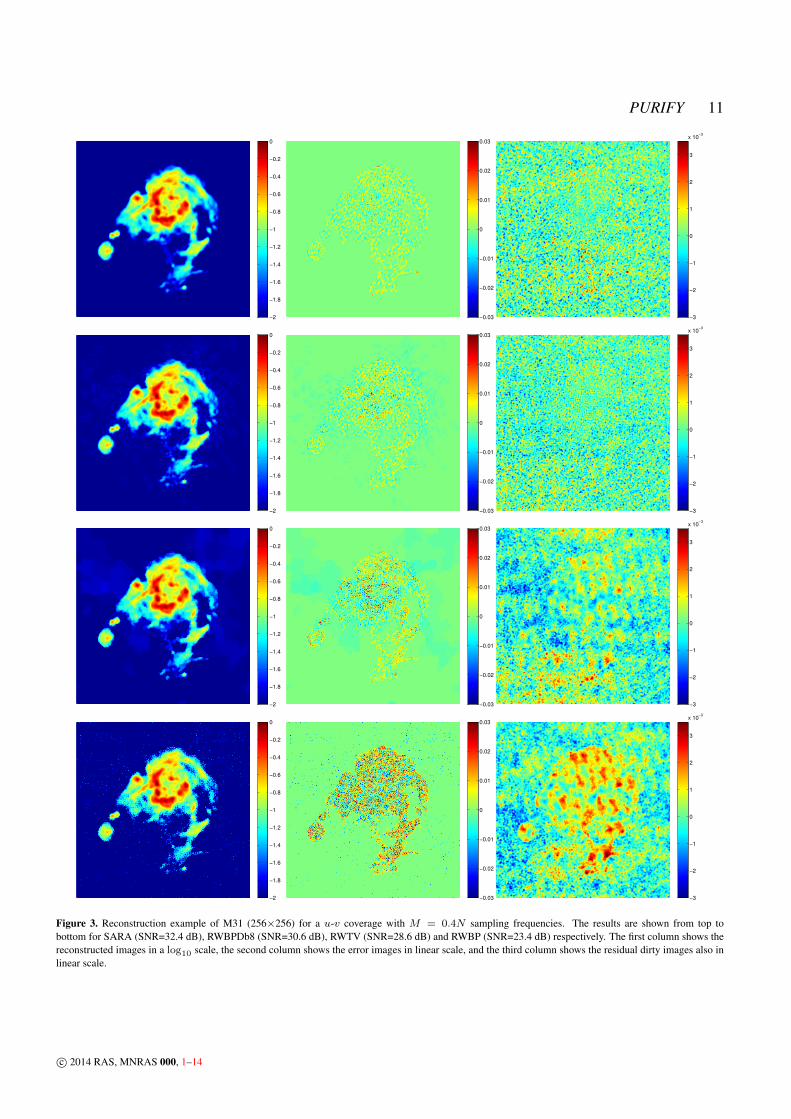