Psychology 205: Research Methods in Psychology Analyzing ... · Preliminaries RecallRecognition...
67
Preliminaries Recall Recognition Inferential Statistics Psychology 205: Research Methods in Psychology Analyzing the memory experiment William Revelle Department of Psychology Northwestern University Evanston, Illinois USA October, 2014 1 / 68
Transcript of Psychology 205: Research Methods in Psychology Analyzing ... · Preliminaries RecallRecognition...

Preliminaries Recall Recognition Inferential Statistics
Psychology 205: Research Methods in PsychologyAnalyzing the memory experiment
William Revelle
Department of PsychologyNorthwestern UniversityEvanston, Illinois USA
October, 2014
1 / 68

Preliminaries Recall Recognition Inferential Statistics
Outline
1 Preliminaries
2 RecallData manipulation and descriptive statisticsInferential StatisticsConclusion from recall
3 Recognition
4 Inferential StatisticsAnalysis of Variance as a generalization of the t-testGraphing the interactions
2 / 68

Preliminaries Recall Recognition Inferential Statistics
Data = Model + Residual (error)
1 Data = Model + Residual
2 Observed data may be represented by a model of the data.What is left over is residual (or error)
3 The process of research is to reduce the residual
4 We do this by a progression of models, ranging from the verysimple to the complex
5 We want to know how each model fits the data
3 / 68

Preliminaries Recall Recognition Inferential Statistics
Consider the Recall and Recognition data
1 How to describe it
Raw dataSummary statisticsGraphically
2 All tables and graphs are prepared by using the R computerpackage. For details on using R, consult the tutorials,particularly the short tutorial, listed in the syllabus
First, install R from http://r-project.org (just do thisonce)Then, install the psych (just do this once)
install.packages(”psych”)
library(psych) #everytime you start R
4 / 68

Preliminaries Recall Recognition Inferential Statistics
The very raw data – as stored in excel
Condition mad fear hate rage temper fury ire wrath happy fight hatred mean calm emotion enrage intrusion whitedark cat charred night funeral color grief blue death ink bottom coal brown gray intrusion butter food eat sandwichrye jam milk flour jelly dough crust slice wine loaf toast intrusion table sit legs seat couch desk recliner sofa woodcushion swivel stool sitting rocking bench intrusion hot snow warm winter ice wet frigid chilly heat weather freezeair shiver Arctic frost intrusion nurse sick lawyer medicine health hospital dentist physician ill patient officestethoscope surgeon clinic cure intrusion shoe hand toe kick sandals soccer yard walk ankle arm boot inch socksmell mouth intrusion apple vegetable orange kiwi citrus ripe pear banana berry cherry basket juice salad bowlcocktail intrusion boy dolls female young dress pretty hair niece dance beautiful cute date aunt daughter sisterintrusion low clouds up tall tower jump above building noon cliff sky over airplane dive elevate intrusion queenEngland crown prince George dictator palace throne chess rule subjects monarch royal leader reign intrusion womanhusband uncle lady mouse male father strong friend beard person handsome muscle suit old intrusion hill valleyclimb summit top molehill peak plain glacier goat bike climber range steep ski intrusion note sound piano sing radioband melody horn concert instrument symphony jazz orchestra art rhythm intrusion thread pin eye sewing sharppoint prick thimble haystack thorn hurt injection syringe cloth knitting intrusion water stream lake Mississippi boattide swim flow run barge creek brook fish bridge winding intrusion2 0 0 0 0 0 0 0 0 0 0 0 0 0 0 0 0 1 1 1 0 1 1 0 1 1 1 1 0 0 1 1 1 1 1 0 0 1 1 1 1 1 1 0 0 1 0 1 1 0 0 0 0 0 0 0 0 0 00 0 0 0 0 0 0 0 0 0 0 0 0 0 0 0 0 0 0 0 0 0 1 1 0 1 0 1 1 1 1 1 1 1 1 1 1 0 1 1 0 1 0 1 0 0 0 0 0 0 0 1 0 0 0 0 0 0 00 0 0 0 0 0 0 0 0 0 0 0 1 1 0 0 0 0 0 0 0 0 0 1 1 1 1 0 0 0 0 0 0 0 0 0 0 0 0 0 0 0 0 0 0 0 0 0 0 0 0 0 0 0 0 0 0 0 00 1 1 1 1 0 0 1 0 1 1 0 1 1 0 1 0 0 0 0 0 0 0 0 1 1 1 1 1 1 1 2 0 0 0 0 0 0 0 0 0 0 0 0 0 0 0 0 0 0 0 0 0 0 0 0 0 0 00 0 0 0 0 1 1 0 0 0 1 0 1 1 0 1 1 0 1 1 11 1 1 1 1 1 0 1 0 1 0 1 1 1 1 1 1 0 0 0 0 0 0 0 0 0 0 0 0 0 0 0 0 0 0 0 0 0 0 0 0 0 0 0 0 0 0 0 0 1 1 1 1 1 1 1 1 1 11 1 1 1 1 0 1 1 1 1 1 0 1 1 1 1 0 0 0 1 1 1 0 0 0 0 0 0 0 0 0 0 0 0 0 0 0 0 0 0 0 0 0 0 0 0 0 0 0 0 0 0 0 0 1 1 1 1 11 1 1 1 1 0 1 1 1 1 0 0 0 0 0 0 0 0 0 0 0 0 0 0 0 0 0 1 1 1 1 1 1 1 1 0 0 1 0 1 1 1 0 1 1 1 1 1 1 1 1 0 0 1 1 1 1 1 00 0 0 0 0 0 0 0 0 0 0 0 0 0 0 0 0 0 0 0 0 0 0 0 0 0 0 0 0 0 0 0 0 0 1 1 0 0 1 1 0 1 1 1 1 1 1 1 1 1 1 1 0 0 0 1 0 1 01 1 0 1 3 0 0 0 0 0 0 0 0 0 0 0 0 0 0 0 01 1 1 0 0 1 1 1 1 1 1 1 1 1 1 1 0 0 0 0 0 0 0 0 0 0 0 0 0 0 0 0 0 0 0 0 0 0 0 0 0 0 0 0 0 0 0 0 0 1 0 1 1 1 1 1 1 1 10 0 0 1 1 0 1 1 1 1 1 0 1 1 1 1 1 1 0 1 1 0 0 0 0 0 0 0 0 0 0 0 0 0 0 0 0 0 0 0 0 0 0 0 0 0 0 0 0 0 0 0 0 0 1 0 1 1 11 1 1 1 1 1 0 1 1 1 0 0 0 0 0 0 0 0 0 0 0 0 0 0 0 0 0 1 1 1 1 1 1 1 1 0 0 1 1 1 1 1 0 1 1 1 1 1 1 1 0 0 0 0 1 1 1 1 00 0 0 0 0 0 0 0 0 0 0 0 0 0 0 0 0 0 0 0 0 0 0 0 0 0 0 0 0 0 0 0 1 1 1 1 1 1 1 1 1 1 1 1 1 1 1 0 0 0 0 1 0 0 1 1 1 0 11 1 0 1 1 0 0 0 0 0 0 0 0 0 0 0 0 0 0 0 0
1 0 0 0 1 0 0 1 0 1 1 0 0 1 0 0 0 0 0 0 0 0 0 0 0 0 0 0 0 0 0 0 0 0 0 0 0 0 0 0 0 0 0 0 0 0 0 0 0 0 0 0 0 0 0 0 1 0 0
1 0 0 1 1 0 0 0 0 0 0 0 0 0 0 0 1 1 1 1 1 0 0 0 0 0 0 0 0 0 0 0 0 0 0 0 0 0 0 0 0 0 0 0 0 0 0 0 0 0 0 0 0 0 1 0 1 1 1
1 1 1 0 0 0 0 0 0 1 0 0 0 0 0 0 0 0 0 0 0 0 0 0 0 0 0 0 1 0 1 0 0 1 1 1 1 0 1 1 1 1 0 1 1 1 1 1 1 1 1 1 1 1 1 1 1 1 0
0 0 0 0 0 0 0 0 0 0 0 0 0 0 0 0 0 0 0 0 0 0 0 0 0 0 0 0 0 0 0 0 1 1 1 0 1 1 1 1 0 1 1 1 1 0 1 0 0 0 1 0 0 0 1 0 1 0 0
0 1 1 1 0 0 0 0 0 0 0 0 0 0 0 0 0 0 0 0 0
5 / 68
Preliminaries Recall Recognition Inferential Statistics
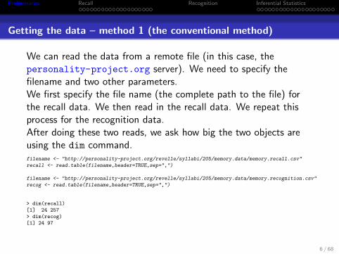
Getting the data – method 1 (the conventional method)
We can read the data from a remote file (in this case, thepersonality-project.org server). We need to specify thefilename and two other parameters.We first specify the file name (the complete path to the file) forthe recall data. We then read in the recall data. We repeat thisprocess for the recognition data.After doing these two reads, we ask how big the two objects areusing the dim command.filename <- "http://personality-project.org/revelle/syllabi/205/memory.data/memory.recall.csv"
recall <- read.table(filename,header=TRUE,sep=",")
filename <- "http://personality-project.org/revelle/syllabi/205/memory.data/memory.recognition.csv"
recog <- read.table(filename,header=TRUE,sep=",")
> dim(recall)
[1] 24 257
> dim(recog)
[1] 24 97
6 / 68

Preliminaries Recall Recognition Inferential Statistics
Getting the data, method 2 (a somewhat easier method)
Alternatively, if you have browser, you can read the remote fileusing our browser and then copy the output into the “clipboard”and then just read the clipboard. This has the advantage that youcan see what you are doing.#first, use your browser to go to
http://personality-project.org/revelle/syllabi/205/memory.data/memory.recall.csv
#copy the resulting window to your clipboard
#read the clipboard
recall <- read.clipboard.csv()
dim(recall)
#then use your browser to go to
http://personality-project.org/revelle/syllabi/205/memory.data/memory.recognition.csv
#copy this to your clipboard and then read the clipboard
recog <- read.clipboard.csv()
dim(recog)
> dim(recall)
[1] 24 257
> dim(recog)
[1] 24 97
These two ways of reading the data are equally easy (complicated).
7 / 68

Preliminaries Recall Recognition Inferential Statistics
Some basic recoding of the data to make it useful
1 Once you have the recall data in the recall object, we need todo some basic recoding to make it useful
We want to find the recall for each position for each subject.The data, as typed in, were in the form of 257 columns foreach of 24 subjects.Condition, List 1, List 2, .... List 16For each list, it went position 1 ... 15 and then the number ofintrusions (false recalls).Thus, we want to add up items 2, 18, 34 ... 242 to get therecall for position 1and then do this for items 3, 19, 35 ... 243 to get recall forposition 2etc.
2 We do this with a bit of code (to be appreciated, and perhapsunderstood).
Create a vector of the first itemUse this to make a matrix of all item positionsThen use that matrix to find the various means
8 / 68

Preliminaries Recall Recognition Inferential Statistics
A bit of strange code (can be appreciated or ignored)
filename <-
recall <- read.clipboard.tab()
dim(recall)
[1] 24 257
W <- seq(2, 257, 16)
W
[1] 2 18 34 50 66 82 98 114 130 146 162
178 194 210 226 242
w <- outer(W,0:15,"+")
w
[1] 2 18 34 50 66 82 98 114 130 146 162 178 194 210 226 242
[,1] [,2] [,3] [,4] [,5] [,6] [,7] [,8] [,9] [,10] [,11] [,12] [,13] [,14] [,15] [,16]
[1,] 2 3 4 5 6 7 8 9 10 11 12 13 14 15 16 17
[2,] 18 19 20 21 22 23 24 25 26 27 28 29 30 31 32 33
[3,] 34 35 36 37 38 39 40 41 42 43 44 45 46 47 48 49
...
[16,] 242 243 244 245 246 247 248 249 250 251 252 253 254 255 256 257
1 First copy the data tothe clipboard andthen read theclipboard into therecall data.frame
2 How big is this dataframe? (What are thedimensions?)
3 Create a vector toshow where each listis
4 Then create a vectorto show how to addup the items
9 / 68

Preliminaries Recall Recognition Inferential Statistics
Data manipulation and descriptive statistics
Find means for each person for each position
rec <- matrix(NA,24,16) #create a matrix to store the results
for (i in 1:16) {rec[,i] <- rowMeans(recall[w[,i]],na.rm=TRUE)*2}
colnames (rec) <- paste0("P",1:16,"")
rownames(rec) <- paste0("S",1:24,"")
rec
P1 P2 P3 P4 P5 P6 P7 P8 P9 P10 P11 P12 P13 P14 P15 P16
S1 0.625 0.875 0.375 0.375 0.375 0.625 0.250 0.625 0.625 0.625 0.625 0.375 0.625 0.875 0.750 0.875
S2 0.875 0.875 1.000 1.000 0.750 0.500 0.875 0.875 0.500 0.625 0.625 0.750 0.875 0.875 1.000 0.750
S3 0.875 0.625 0.750 0.875 0.875 0.750 1.000 0.875 0.750 0.625 0.750 0.750 0.750 0.875 1.000 0.125
S4 0.375 0.375 0.500 0.500 0.375 0.375 0.750 0.625 0.500 0.500 0.500 0.500 0.750 0.625 0.875 0.000
S5 0.875 1.000 0.875 0.750 0.750 0.625 0.750 1.000 0.625 0.750 0.750 0.625 0.625 0.750 0.375 0.375
S6 1.000 1.000 1.000 0.750 0.750 0.500 0.625 0.625 0.375 0.625 0.750 0.375 0.500 0.875 0.875 0.875
S7 0.875 0.750 0.750 1.000 0.750 0.500 0.500 0.250 0.250 0.250 0.625 0.625 0.750 0.750 0.750 0.000
S8 0.875 0.875 0.625 0.875 0.625 0.625 0.500 0.375 0.750 0.875 0.375 0.625 0.875 0.875 0.625 0.750
S9 0.750 0.750 0.625 0.750 0.625 0.875 0.875 0.750 0.750 0.875 0.875 0.875 0.750 1.000 1.000 1.000
S10 0.875 1.000 0.875 0.750 0.750 0.875 0.625 0.625 0.750 0.500 0.750 0.875 0.750 0.750 1.000 0.000
S11 1.000 1.000 0.750 0.750 0.750 0.750 0.625 0.750 0.500 0.500 0.625 0.625 0.750 1.000 0.875 0.500
S12 0.875 0.875 1.000 1.000 0.875 1.000 1.000 1.000 1.000 0.875 0.875 0.875 0.750 1.000 1.000 0.125
S13 1.000 0.875 0.875 0.500 0.625 0.875 0.750 0.625 0.500 0.625 0.625 0.625 0.750 0.875 0.875 0.800
S14 0.875 0.750 0.750 0.750 0.625 0.750 0.500 0.750 1.000 0.625 0.500 0.625 0.500 0.875 1.000 0.750
S15 1.000 1.000 1.000 0.750 0.625 0.625 0.625 0.750 0.750 0.500 0.500 0.750 0.875 1.000 0.875 0.125
S16 1.000 0.750 0.750 0.750 0.375 0.875 0.750 0.750 0.625 0.500 0.625 0.750 0.625 0.625 0.750 1.500
S17 0.875 0.875 0.750 0.875 1.000 0.625 0.625 0.750 0.625 0.625 1.000 0.500 1.000 0.750 0.875 1.375
S18 0.750 0.875 0.875 0.875 0.625 0.875 0.625 0.250 0.250 0.500 0.125 0.250 0.625 0.875 1.000 0.250
S19 0.750 0.875 0.875 0.750 0.625 0.750 0.875 0.875 0.625 1.000 0.875 0.875 0.875 0.875 0.875 0.125
S20 1.000 0.875 0.875 1.000 1.000 0.625 0.875 0.500 0.750 0.375 0.500 0.500 0.625 0.500 1.000 0.250
S21 0.875 0.750 0.625 0.750 0.875 0.500 0.625 0.875 0.250 0.875 0.500 0.375 0.750 0.875 0.750 0.250
S22 0.750 0.750 0.750 0.875 0.500 0.625 0.875 0.500 0.625 0.625 0.500 0.250 0.500 0.625 0.625 1.500
S23 1.000 0.875 0.750 0.750 0.750 0.625 0.750 0.500 0.750 0.750 0.625 0.500 1.000 0.750 0.750 0.375
S24 1.000 0.750 0.750 0.875 0.750 0.875 0.750 0.625 0.750 0.750 0.750 0.625 0.875 0.500 0.875 0.000
10 / 68

Preliminaries Recall Recognition Inferential Statistics
Data manipulation and descriptive statistics
Show the data by person and by list: Is there a pattern?
2 4 6 8 10 12 14
0.0
0.2
0.4
0.6
0.8
1.0
Recall by person and list
Pro
babi
lity
of re
call
11 / 68

Preliminaries Recall Recognition Inferential Statistics
Data manipulation and descriptive statistics
Describe the Position data (remember, position 16 is actually theintrusions.
> describe(rec)
vars n mean sd median trimmed mad min max range skew kurtosis se
P1 1 24 0.86 0.15 0.88 0.89 0.19 0.38 1.00 0.62 -1.54 2.71 0.03
P2 2 24 0.83 0.14 0.88 0.85 0.19 0.38 1.00 0.62 -1.27 2.27 0.03
P3 3 24 0.78 0.16 0.75 0.79 0.19 0.38 1.00 0.62 -0.58 0.04 0.03
P4 4 24 0.79 0.16 0.75 0.80 0.19 0.38 1.00 0.62 -0.78 0.36 0.03
P5 5 24 0.69 0.17 0.75 0.69 0.19 0.38 1.00 0.62 -0.22 -0.51 0.04
P6 6 24 0.69 0.16 0.62 0.69 0.19 0.38 1.00 0.62 0.03 -1.03 0.03
P7 7 24 0.71 0.18 0.75 0.71 0.19 0.25 1.00 0.75 -0.42 0.01 0.04
P8 8 24 0.67 0.20 0.69 0.68 0.19 0.25 1.00 0.75 -0.41 -0.53 0.04
P9 9 24 0.62 0.20 0.62 0.62 0.19 0.25 1.00 0.75 -0.23 -0.46 0.04
P10 10 24 0.64 0.18 0.62 0.64 0.19 0.25 1.00 0.75 0.05 -0.52 0.04
P11 11 24 0.64 0.19 0.62 0.64 0.19 0.12 1.00 0.88 -0.43 0.46 0.04
P12 12 24 0.60 0.19 0.62 0.61 0.19 0.25 0.88 0.62 -0.23 -0.98 0.04
P13 13 24 0.74 0.14 0.75 0.74 0.19 0.50 1.00 0.50 -0.01 -0.81 0.03
P14 14 24 0.81 0.15 0.88 0.82 0.19 0.50 1.00 0.50 -0.59 -0.62 0.03
P15 15 24 0.85 0.16 0.88 0.87 0.19 0.38 1.00 0.62 -1.16 1.20 0.03
P16 16 24 0.53 0.48 0.38 0.48 0.56 0.00 1.50 1.50 0.66 -0.81 0.10
12 / 68

Preliminaries Recall Recognition Inferential Statistics
Data manipulation and descriptive statistics
It is hard to see patterns from tables of numbers. Show the datagraphically
1 The first graphic compares the means and the medians.
Medians are less sensitive to outliers than are the meansThere two do not differ very much
2 But we really want to know if the recall numbers differ as afunction of position
3 There are several ways of showing this graphically
A boxplota simple line graphA line graph with error bars
13 / 68

Preliminaries Recall Recognition Inferential Statistics
Data manipulation and descriptive statistics
A simple boxplot
boxplot(rec[,1:15],ylab=”recall”,xlab=”position”,main=”Boxplot ofrecall by postion”,ylim=c(0,1))
1 2 3 4 5 6 7 8 9 10 11 12 13 14 15
0.0
0.2
0.4
0.6
0.8
1.0
Boxplot of recall by postion
position
recall
14 / 68

Preliminaries Recall Recognition Inferential Statistics
Data manipulation and descriptive statistics
Plot some summary estimates of central tendency; Is there apattern?
2 4 6 8 10 12 14
0.0
0.2
0.4
0.6
0.8
1.0
Mean and Median probability of recall by list
Position
mea
n an
d m
edia
n
15 / 68

Preliminaries Recall Recognition Inferential Statistics
Data manipulation and descriptive statistics
Means and their standard errors
1 The mean of any set of observations represents the samplemean.
2 If we were to take other samples from the same population,we would probably find a different mean
3 The variation from one sample to another can be predictedbased upon the population standard deviation
The central limit theorem says that the distribution of samplemeans should tend towards normal with a standard deviationof the means (the standard error or the mean, or the standarderror)
σ2x = σ2
N <==> σx = σx√N
The standard error of a mean is the sample standard deviationdivided by the square root of the sample size
16 / 68

Preliminaries Recall Recognition Inferential Statistics
Data manipulation and descriptive statistics
Showing means and their standard errors
1 When graphing a mean or a set of means, one should alsoshow the standard error of those means.
Typically, this is done by showing the mean ±1.96 standarderror
2 More recently, it has been pointed out that the likelihood ofthe mean is not distributed equally throughout the range, butis more likely towards the middle of the confidence range.
3 This has led to the use of “cat’s eye plots”
4 Both kind of plots can be done using the error.bars function
17 / 68

Preliminaries Recall Recognition Inferential Statistics
Data manipulation and descriptive statistics
The recall data show a serial position– add in the standard errors
error.bars(rec[,1:15],ylab=”recall”,xlab=”position”,main=”meansand errorbars of recall bypostion”,ylim=c(0,1),type=”l”,eyes=FALSE)
means and errorbars of recall by postion
position
recall
1 2 3 4 5 6 7 8 9 10 11 12 13 14 15
0.0
0.2
0.4
0.6
0.8
1.0
18 / 68

Preliminaries Recall Recognition Inferential Statistics
Data manipulation and descriptive statistics
The recall data show a serial position– add in the standard errors
error.bars(rec[,1:15],ylab=”recall”,xlab=”position”,main=”meansand errorbars of recall by postion”,ylim=c(0,1),type=”l”)
95% confidence limits
Serial Position
Pro
babi
lity
of R
ecal
l
P1 P2 P3 P4 P5 P6 P7 P8 P9 P10 P11 P12 P13 P14 P15
0.0
0.2
0.4
0.6
0.8
1.0
19 / 68

Preliminaries Recall Recognition Inferential Statistics
Data manipulation and descriptive statistics
The two groups do not seem to differ
error.bars.by(rec[,1:15],group=recall$Condition,ylab=”recall”,xlab=”position”,main=”means and errorbars of recall by position”,ylim=c(0,1))abline(h=.53/8)
text(3,.1,”Intrusions”)
means and errorbars of recall by position
position
recall
1 2 3 4 5 6 7 8 9 10 11 12 13 14 15
0.0
0.2
0.4
0.6
0.8
1.0
Intrusions
20 / 68

Preliminaries Recall Recognition Inferential Statistics
Data manipulation and descriptive statistics
Data = Model + Residual (error)
1 Data = Model + Residual
2 Observed data may be represented by a model of the data.What is left over is residual (or error)
3 The process of research is to reduce the residual
4 We do this by a progression of models, ranging from the verysimple to the complex
5 We want to know how each model fits the data
21 / 68

Preliminaries Recall Recognition Inferential Statistics
Data manipulation and descriptive statistics
People are a major source of difference
People differ in their probability of endorsement
Participant
Pro
babi
lity
of R
ecal
l
S1 S2 S3 S4 S5 S6 S7 S8 S9 S11 S13 S15 S17 S19 S21 S23
0.0
0.2
0.4
0.6
0.8
1.0
22 / 68
Preliminaries Recall Recognition Inferential Statistics
Data manipulation and descriptive statistics
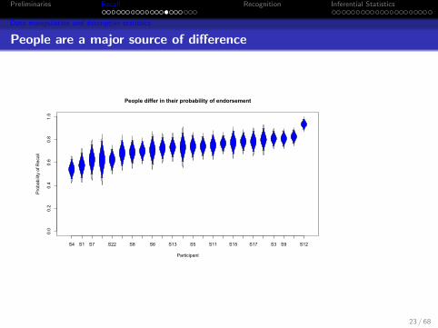
People are a major source of difference
People differ in their probability of endorsement
Participant
Pro
babi
lity
of R
ecal
l
S4 S1 S7 S22 S8 S6 S13 S5 S11 S15 S17 S3 S9 S12
0.0
0.2
0.4
0.6
0.8
1.0
23 / 68

Preliminaries Recall Recognition Inferential Statistics
Data manipulation and descriptive statistics
R code for person graphs — supplementary information
R is a syntax driven language, but each line of syntax is prettystraightforward. This is shown here for demonstration purposes onhow to draw some graphs using some of the built in functions.#first, plot the means and medians
plot(colMeans(rec[,1:15]),ylim=c(0,1),ylab="mean and median",xlab="Position",
main="Mean and Median probability of recall by list",type="b")
points(apply(rec[,1:15],2,median)
,type="b",lty="dashed")
#now show the error bars
error.bars(t(rec[,1:15]),ylab="Probability of Recall",ylim=c(0,1),
xlab="Participant",main="People differ in their probability of endorsement")
#show them by group
error.bars.by(rec[,1:15],group=recall$Condition,ylim=c(0,1),
ylab="Probability of Recall",xlab="Serial Position")
#plot by person rather than by item (this is plotting the matrix transpose)
error.bars(t(rec[,1:15]),ylab="Probability of Recall",ylim=c(0,1),
xlab="Participant",main="People differ in their probability of endorsement")
#find the individual total scores
tot <- rowSums(rec[,1:15])
ord <- order(tot)
#plot subjects ordered by total score
error.bars(t(rec[ord,1:15]),ylab="Probability of Recall",ylim=c(0,1),xlab=
"Participant",main="People differ in their probability of endorsement")
24 / 68
Preliminaries Recall Recognition Inferential Statistics
Data manipulation and descriptive statistics
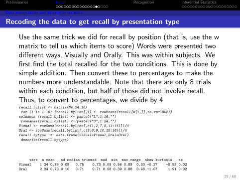
Recoding the data to get recall by presentation type
Use the same trick we did for recall by position (that is, use the wmatrix to tell us which items to score) Words were presented twodifferent ways, Visually and Orally. This was within subjects. Wefirst find the total recalled for the two conditions. This is done bysimple addition. Then convert these to percentages to make thenumbers more understandable. Note that there are only 8 trialswithin each condition, but half of those did not involve recall.Thus, to convert to percentages, we divide by 4recall.bylist <- matrix(NA,24,16)
for (i in 1:16) {recall.bylist[,i] <- rowMeans(recall[w[i,]],na.rm=TRUE)}
colnames (recall.bylist) <- paste0("L",1:16,"")
rownames(recall.bylist) <- paste0("S",1:24,"")
Visual <- rowSums(recall.bylist[,c(1,2,7,8,11:14)])/4
Oral <- rowSums(recall.bylist[,c(3:6,9,10,15:16)])/4
recall.bytype <- data.frame(Visual=Visual,Oral=Oral)
describe(recall.bytype)
vars n mean sd median trimmed mad min max range skew kurtosis se
Visual 1 24 0.73 0.09 0.75 0.73 0.09 0.56 0.89 0.33 -0.27 -0.83 0.02
Oral 2 24 0.70 0.10 0.71 0.71 0.08 0.39 0.88 0.48 -1.07 1.91 0.02
25 / 68

Preliminaries Recall Recognition Inferential Statistics
Data manipulation and descriptive statistics
Recall by Visual and Oral presentation condition
Recall by condition
Condition
Recall
Visual Oral
0.0
0.2
0.4
0.6
0.8
1.0
26 / 68

Preliminaries Recall Recognition Inferential Statistics
Inferential Statistics
The t-test
Developed by “student” (William Gosset)
A small sample extension of the z-test for comparing twogroupsLike most statistics, what is the size of the effect versus theerror of the effect?
Standard error of a mean is s.e. = σx =√
σ2
N
Two casesIndependent groups
t = X1−X2√σ2
1/N1+σ22/N2
degrees of freedom df = N1 − 1 + N2 − 1
Paired differences (correlated groups)
let d = X1 − X2 then t = dσd
d.f. = N - 1
done in R with t.test function
27 / 68

Preliminaries Recall Recognition Inferential Statistics
Inferential Statistics
Does Recall differ by modality of presentation? The paired t-test.
Visual <- rowSums(recall.bylist[,c(1,2,7,8,11:14)])/4
Oral <- rowSums(recall.bylist[,c(3:6,9,10,15:16)])/4
recall.bytype <- data.frame(Visual=Visual,Oral=Oral)
describe(recall.bytype)
> with(recall.bytype,t.test(Visual,Oral,paired=TRUE))
vars n mean sd median trimmed mad min max range skew kurtosis se
Visual 1 24 0.73 0.09 0.75 0.73 0.09 0.56 0.89 0.33 -0.27 -0.83 0.02
Oral 2 24 0.70 0.10 0.71 0.71 0.08 0.39 0.88 0.48 -1.07 1.91 0.02
Paired t-test
data: Visual and Oral
t = 1.6312, df = 23, p-value = 0.1165
alternative hypothesis: true difference in means is not equal to 0
95 percent confidence interval:
-0.007390829 0.062512357
sample estimates:
mean of the differences
0.02756076
Mean recall does not differ as a function of modality ofpresentation.
28 / 68

Preliminaries Recall Recognition Inferential Statistics
Conclusion from recall
Recall results
As predicted, there was a serial position effect.
This suggested that the participants followed instructions.
There was no difference between the serial position effects forthe two experimental groups.
There was no effect of modality of presentation on immediaterecall.
Now need to see if there is a false memory effect onsubsequent recognition.
29 / 68
Preliminaries Recall Recognition Inferential Statistics
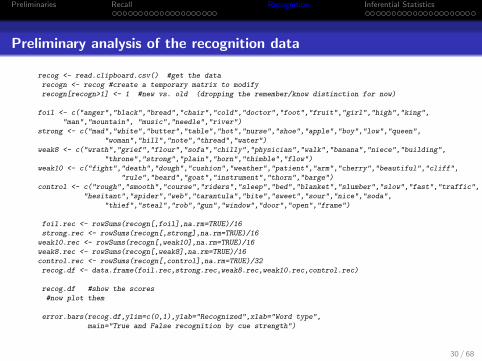
Preliminary analysis of the recognition data
recog <- read.clipboard.csv() #get the data
recogn <- recog #create a temporary matrix to modify
recogn[recogn>1] <- 1 #new vs. old (dropping the remember/know distinction for now)
foil <- c("anger","black","bread","chair","cold","doctor","foot","fruit","girl","high","king",
"man","mountain", "music","needle","river")
strong <- c("mad","white","butter","table","hot","nurse","shoe","apple","boy","low","queen",
"woman","hill","note","thread","water")
weak8 <- c("wrath","grief","flour","sofa","chilly","physician","walk","banana","niece","building",
"throne","strong","plain","horn","thimble","flow")
weak10 <- c("fight","death","dough","cushion","weather","patient","arm","cherry","beautiful","cliff",
"rule","beard","goat","instrument","thorn","barge")
control <- c("rough","smooth","course","riders","sleep","bed","blanket","slumber","slow","fast","traffic",
"hesitant","spider","web","tarantula","bite","sweet","sour","nice","soda",
"thief","steal","rob","gun","window","door","open","frame")
foil.rec <- rowSums(recogn[,foil],na.rm=TRUE)/16
strong.rec <- rowSums(recogn[,strong],na.rm=TRUE)/16
weak10.rec <- rowSums(recogn[,weak10],na.rm=TRUE)/16
weak8.rec <- rowSums(recogn[,weak8],na.rm=TRUE)/16
control.rec <- rowSums(recogn[,control],na.rm=TRUE)/32
recog.df <- data.frame(foil.rec,strong.rec,weak8.rec,weak10.rec,control.rec)
recog.df #show the scores
#now plot them
error.bars(recog.df,ylim=c(0,1),ylab="Recognized",xlab="Word type",
main="True and False recognition by cue strength")
30 / 68

Preliminaries Recall Recognition Inferential Statistics
Show the scores
recog.df #show the scores
foil.rec strong.rec weak8.rec weak10.rec control.rec
1 0.6875 0.7500 0.6875 0.5625 0.00000
2 0.4375 1.0000 1.0000 0.9375 0.00000
3 0.4375 0.6250 0.6250 0.5625 0.37500
4 0.5625 0.8125 0.8125 0.8750 0.28125
5 0.3125 0.9375 0.9375 0.8750 0.03125
6 0.6250 0.8750 0.6875 0.7500 0.06250
7 0.6875 0.8750 0.8750 0.7500 0.31250
8 0.9375 0.7500 0.6875 0.6875 0.03125
9 0.6875 0.9375 1.0000 1.0000 0.18750
10 0.0625 0.8750 0.6875 0.7500 0.00000
11 0.6875 0.9375 0.8750 0.7500 0.09375
12 0.3125 0.8750 0.8750 0.9375 0.00000
13 0.4375 0.8125 0.8125 0.8750 0.03125
14 0.4375 0.7500 0.6250 0.6875 0.59375
15 0.5000 0.8125 0.8125 0.6250 0.00000
16 0.8750 0.9375 0.8125 0.6875 0.00000
17 0.2500 1.0000 0.8750 0.9375 0.00000
18 0.4375 0.8125 0.4375 0.5625 0.06250
19 0.6250 0.9375 0.8125 0.6875 0.03125
20 0.0000 0.5000 0.6875 0.6250 0.00000
21 0.5625 0.9375 0.8125 0.8750 0.18750
22 0.6875 0.9375 0.6875 0.6250 0.00000
23 0.3750 0.7500 0.8125 0.9375 0.03125
24 0.3750 0.8750 0.8750 0.8750 0.12500
31 / 68

Preliminaries Recall Recognition Inferential Statistics
Boxplot of recognition data
boxplot(recog.df,ylab=”Recognition”,main=”True and FalseRecognition”)
foil.rec strong.rec weak8.rec weak10.rec control.rec
0.0
0.2
0.4
0.6
0.8
1.0
True and False Recognition
Recognition
32 / 68
Preliminaries Recall Recognition Inferential Statistics
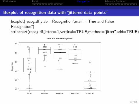
Boxplot of recognition data with “jittered data points”
boxplot(recog.df,ylab=”Recognition”,main=”True and FalseRecognition”)stripchart(recog.df,jitter=.1,vertical=TRUE,method=”jitter”,add=TRUE)
foil.rec strong.rec weak8.rec weak10.rec control.rec
0.0
0.2
0.4
0.6
0.8
1.0
True and False Recognition
Recognition
33 / 68

Preliminaries Recall Recognition Inferential Statistics
Descriptive stats of recognition
describe(recog.df)
vars n mean sd median trimmed mad min max range skew kurtosis se
foil.rec 1 24 0.50 0.23 0.47 0.51 0.23 0.00 0.94 0.94 -0.25 -0.28 0.05
strong.rec 2 24 0.85 0.12 0.88 0.86 0.09 0.50 1.00 0.50 -1.10 1.03 0.02
weak8.rec 3 24 0.78 0.13 0.81 0.79 0.14 0.44 1.00 0.56 -0.51 0.10 0.03
weak10.rec 4 24 0.77 0.14 0.75 0.77 0.19 0.56 1.00 0.44 0.01 -1.46 0.03
control.rec 5 24 0.10 0.15 0.03 0.07 0.05 0.00 0.59 0.59 1.73 2.38 0.03
34 / 68
Preliminaries Recall Recognition Inferential Statistics
Further recoding
1 Words were presented two different ways
VisualOral
2 Some lists were recalled, some were not– does this make adifference
Recall if A Math if B
3 This requires some recoding of the data
35 / 68
Preliminaries Recall Recognition Inferential Statistics
Do some recoding of the data
cued <- matrix(c(foil,strong,weak8,weak10),ncol=4)
cued.rec <- matrix(NA,24,4)
for(i in 1:4) {cued.rec[,i] <- rowSums(recogn[,cued[,i]],na.rm=TRUE)}
cued.recv <- matrix(NA,24,4)
cued.v <- cued[vo==1,]
cued.o <- cued[vo==2,]
cued.va <- cued[((vo==1) & (ab==1)),]
cued.vb <- cued[((vo==1) & (ab==2)),]
cued.oa <- cued[((vo==2) & (ab==1)),]
cued.ob <- cued[((vo==2) & (ab==2)),]
cued.rec <- matrix(NA,24,16)
for(i in 1:4) {cued.rec[,i] <- rowSums(recogn[,cued.va[,i]],na.rm=TRUE)}
for(i in 1:4) {cued.rec[,i+4] <- rowSums(recogn[,cued.vb[,i]],na.rm=TRUE)}
for(i in 1:4) {cued.rec[,i+8] <- rowSums(recogn[,cued.oa[,i]],na.rm=TRUE)}
for(i in 1:4) {cued.rec[,i+12] <- rowSums(recogn[,cued.ob[,i]],na.rm=TRUE)}
colnames(cued.rec) <- c("FoilVa","StrongVA","WeakVa","WeakerVA","FoilVb",
"StrongVb","WeakVb","WeakerVb","FoilOa","StrongOA","WeakOa",
"WeakerOa","FoilOb","StrongOb","WeakOb","WeakerVOb")
rownames(cued.rec) <- paste("S",1:24,sep="")
describeBy(cued.rec/4,group=recog$Condition)
error.bars.by(cued.rec/4,recog$Condition,ylab="Recognition",xlab="Within Person Condition",main="Recognition by word location and A/B condition")
36 / 68

Preliminaries Recall Recognition Inferential Statistics
Check the coding
> cued.va
[,1] [,2] [,3] [,4]
[1,] "anger" "mad" "wrath" "fight"
[2,] "fruit" "apple" "banana" "cherry"
[3,] "king" "queen" "throne" "rule"
[4,] "music" "note" "horn" "instrument"
> cued.vb
[,1] [,2] [,3] [,4]
[1,] "black" "white" "grief" "death"
[2,] "foot" "shoe" "walk" "arm"
[3,] "man" "woman" "strong" "beard"
[4,] "mountain" "hill" "plain" "goat"
> cued.oa
[,1] [,2] [,3] [,4]
[1,] "chair" "table" "sofa" "cushion"
[2,] "cold" "hot" "chilly" "weather"
[3,] "high" "low" "building" "cliff"
[4,] "needle" "thread" "thimble" "thorn"
> cued.ob
[,1] [,2] [,3] [,4]
[1,] "bread" "butter" "flour" "dough"
[2,] "doctor" "nurse" "physician" "patient"
[3,] "girl" "boy" "niece" "beautiful"
[4,] "river" "water" "flow" "barge"37 / 68

Preliminaries Recall Recognition Inferential Statistics
The A condition
INDICES: 1
vars n mean sd median trimmed mad min max range skew kurtosis se
FoilVa 1 13 0.37 0.28 0.25 0.36 0.37 0.00 0.75 0.75 0.09 -1.52 0.08
StrongVA 2 13 0.88 0.13 1.00 0.89 0.00 0.75 1.00 0.25 -0.14 -2.13 0.04
WeakVa 3 13 0.83 0.19 0.75 0.84 0.37 0.50 1.00 0.50 -0.48 -1.24 0.05
WeakerVA 4 13 0.71 0.27 0.75 0.73 0.37 0.25 1.00 0.75 -0.48 -1.15 0.07
FoilVb 5 13 0.54 0.35 0.50 0.55 0.37 0.00 1.00 1.00 -0.42 -1.23 0.10
StrongVb 6 13 0.85 0.24 1.00 0.89 0.00 0.25 1.00 0.75 -1.26 0.36 0.07
WeakVb 7 13 0.62 0.30 0.50 0.64 0.37 0.00 1.00 1.00 -0.32 -0.82 0.08
WeakerVb 8 13 0.77 0.26 0.75 0.80 0.37 0.25 1.00 0.75 -0.55 -1.21 0.07
FoilOa 9 13 0.56 0.31 0.50 0.57 0.37 0.00 1.00 1.00 -0.16 -1.26 0.09
StrongOA 10 13 0.79 0.22 0.75 0.80 0.37 0.50 1.00 0.50 -0.27 -1.80 0.06
WeakOa 11 13 0.85 0.19 1.00 0.86 0.00 0.50 1.00 0.50 -0.66 -1.13 0.05
WeakerOa 12 13 0.75 0.23 0.75 0.77 0.37 0.25 1.00 0.75 -0.61 -0.56 0.06
FoilOb 13 13 0.54 0.34 0.50 0.55 0.37 0.00 1.00 1.00 0.12 -1.48 0.09
StrongOb 14 13 0.81 0.21 0.75 0.84 0.00 0.25 1.00 0.75 -1.19 1.26 0.06
WeakOb 15 13 0.81 0.18 0.75 0.82 0.37 0.50 1.00 0.50 -0.31 -1.23 0.05
WeakerVOb 16 13 0.81 0.18 0.75 0.82 0.37 0.50 1.00 0.50 -0.31 -1.23 0.05
38 / 68

Preliminaries Recall Recognition Inferential Statistics
The B condition
------------------------------------------------------------------------------------------r----------------------------
INDICES: 2
vars n mean sd median trimmed mad min max range skew kurtosis se
FoilVa 1 11 0.43 0.23 0.50 0.44 0.37 0.00 0.75 0.75 -0.26 -0.96 0.07
StrongVA 2 11 0.86 0.26 1.00 0.92 0.00 0.25 1.00 0.75 -1.36 0.28 0.08
WeakVa 3 11 0.80 0.19 0.75 0.81 0.37 0.50 1.00 0.50 -0.25 -1.37 0.06
WeakerVA 4 11 0.70 0.29 0.75 0.72 0.37 0.25 1.00 0.75 -0.37 -1.51 0.09
FoilVb 5 11 0.41 0.36 0.50 0.39 0.37 0.00 1.00 1.00 0.40 -1.18 0.11
StrongVb 6 11 0.98 0.08 1.00 1.00 0.00 0.75 1.00 0.25 -2.47 4.52 0.02
WeakVb 7 11 0.82 0.20 0.75 0.83 0.37 0.50 1.00 0.50 -0.43 -1.41 0.06
WeakerVb 8 11 0.73 0.18 0.75 0.72 0.00 0.50 1.00 0.50 0.09 -1.16 0.05
FoilOa 9 11 0.68 0.28 0.75 0.69 0.37 0.25 1.00 0.75 -0.33 -1.39 0.08
StrongOA 10 11 0.84 0.17 0.75 0.86 0.37 0.50 1.00 0.50 -0.44 -1.08 0.05
WeakOa 11 11 0.80 0.25 0.75 0.83 0.37 0.25 1.00 0.75 -0.90 -0.37 0.07
WeakerOa 12 11 0.82 0.20 0.75 0.83 0.37 0.50 1.00 0.50 -0.43 -1.41 0.06
FoilOb 13 11 0.48 0.26 0.50 0.47 0.00 0.00 1.00 1.00 0.16 -0.31 0.08
StrongOb 14 11 0.77 0.13 0.75 0.78 0.00 0.50 1.00 0.50 0.11 -0.01 0.04
WeakOb 15 11 0.77 0.18 0.75 0.78 0.00 0.50 1.00 0.50 -0.09 -1.16 0.05
WeakerVOb 16 11 0.86 0.17 1.00 0.89 0.00 0.50 1.00 0.50 -0.69 -0.89 0.05
39 / 68

Preliminaries Recall Recognition Inferential Statistics
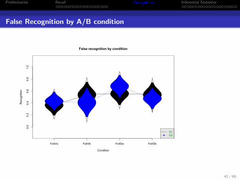
That is too complicated, lets just look at the foils, first the numbers,then the graph
describeBy(cued.rec[,c(1,5,9,13)]/4,group=recog$Condition)
error.bars.by(cued.rec[,c(1,5,9,13)]/4,group=recog$Condition,legend=1,
ylab="Recognition",xlab="Condition",main="False recognition by condition")
INDICES: 1
vars n mean sd median trimmed mad min max range skew kurtosis se
FoilVa 1 13 0.37 0.28 0.25 0.36 0.37 0 0.75 0.75 0.09 -1.52 0.08
FoilVb 2 13 0.54 0.35 0.50 0.55 0.37 0 1.00 1.00 -0.42 -1.23 0.10
FoilOa 3 13 0.56 0.31 0.50 0.57 0.37 0 1.00 1.00 -0.16 -1.26 0.09
FoilOb 4 13 0.54 0.34 0.50 0.55 0.37 0 1.00 1.00 0.12 -1.48 0.09
----------------------------------------------------------------------------------------------------------------------
INDICES: 2
vars n mean sd median trimmed mad min max range skew kurtosis se
FoilVa 1 11 0.43 0.23 0.50 0.44 0.37 0.00 0.75 0.75 -0.26 -0.96 0.07
FoilVb 2 11 0.41 0.36 0.50 0.39 0.37 0.00 1.00 1.00 0.40 -1.18 0.11
FoilOa 3 11 0.68 0.28 0.75 0.69 0.37 0.25 1.00 0.75 -0.33 -1.39 0.08
FoilOb 4 11 0.48 0.26 0.50 0.47 0.00 0.00 1.00 1.00 0.16 -0.31 0.08
40 / 68
Preliminaries Recall Recognition Inferential Statistics
False Recognition by A/B condition
False recognition by condition
Condition
Recognition
FoilVa FoilVb FoilOa FoilOb
0.0
0.2
0.4
0.6
0.8
1.0
G1G2
41 / 68

Preliminaries Recall Recognition Inferential Statistics
Descriptive versus inferential
Descriptive statistics is also known as Exploratory DataAnalysis; Analogous to a detective trying to solve a crime
We are acting as a detective, trying to understand what isgoing onLooking for strange behaviorsDeveloping hypotheses (ideally hypotheses are developedbefore collecting data, but it is important for future studies toexamine the current data to develop hypotheses)
This is in contrast to Inferential Statistics; analogous to acourt proceeding with the presumption of innocence.
Are the results different enough from what is expected by asimpler hypothesis to reject that simpler hypothesis.A typical “simple” hypothesis is the “Null Hypothesis” (aka“Nill” hypothesis).What is the likelihood of observing our data given the Nullhypothesis versus our alternative hypothesis.
What do the data show? How certain are we that they showit? 42 / 68

Preliminaries Recall Recognition Inferential Statistics
Inferential tests: t, F, r
The basic inferential test is the t-test.Is the difference between two group means larger thanexpected by chance?“Nill hypothesis” is that two groups are both sampled from thesame population.Alternative hypothesis is that the two groups come fromdifferent populations with different means.
The basic test was developed by William Gosset (publishingunder the pseudonym of “student”)Two cases
Independent groups
t = X1−X2√σ2
1/N1+σ22/N2
degrees of freedom df = N1 − 1 + N2 − 1
Paired differences (correlated groups)
let d = X1 − X2 then t = dσd
d.f. = N - 1
43 / 68

Preliminaries Recall Recognition Inferential Statistics
Hypothesis testing using inferential statistics
How likely are the observed data given the hypothesis that anIndependent Variable has no effect.Bayesian statistics compare the likelihood of the data giventhe hypothesis of no differences as contrasted to the likelihoodof the data given competing hypotheses.
This takes into account our prior willingness to believe that theIV could have an effect.Also takes into account our strength of belief in the hypothesisof no effect
Conventional tests report the probability of the data given the“Null” hypothesis of no difference.The less likely the data are to be observed given the Null, themore we tend to discount the Null.
Three kinds of inferential errors: Type I, Type II and Type IIIType I is rejecting the Null when in fact it is trueType II is failing to reject the Null when it is in fact not trueType III is asking the wrong question 44 / 68

Preliminaries Recall Recognition Inferential Statistics
Hypothesis Testing
Table : The ways we can be mistaken
State of the World
True False
Scientists says True Valid Positive Type I error
False Type II error Valid rejection
Type III error is asking the wrong question!
45 / 68

Preliminaries Recall Recognition Inferential Statistics
Error probability depends upon the base rates as well
1 The less likely the finding, the more likely a ”significantfinding” is actually a type I error
Table : The ways we can be mistaken
State of the World
True False Total
Scientists says True 475 25 500
False 25 475 500
Total 500 500 1000
46 / 68
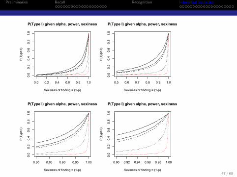
Preliminaries Recall Recognition Inferential Statistics
0.0 0.2 0.4 0.6 0.8 1.0
0.0
0.2
0.4
0.6
0.8
1.0
P(Type I) given alpha, power, sexiness
Sexiness of finding = (1-p)
P(T
ype
I)
0.5 0.6 0.7 0.8 0.9 1.0
0.0
0.2
0.4
0.6
0.8
1.0
P(Type I) given alpha, power, sexiness
Sexiness of finding = (1-p)
P(T
ype
I)
0.80 0.85 0.90 0.95 1.00
0.0
0.2
0.4
0.6
0.8
1.0
P(Type I) given alpha, power, sexiness
Sexiness of finding = (1-p)
P(T
ype
I)
0.90 0.92 0.94 0.96 0.98 1.00
0.0
0.2
0.4
0.6
0.8
1.0
P(Type I) given alpha, power, sexiness
Sexiness of finding = (1-p)
P(T
ype
I)
47 / 68

Preliminaries Recall Recognition Inferential Statistics
Analysis of Variance as a generalization of the t-test
Analysis of Variance allows for testing multiple hypotheses at once
The t-test compares group means to the standard error oftheir differencesThe F-test (developed by R. A. Fisher) compares the variancesbetween group means to the variance within groups.
For two groups, F is just t2, but the theory generalizes tomultiple groups.
The F is a ratio of variances: VarianceBetweenGroupsVariancewithingroups =
σ2bg
σ2wg
To make this sound more complicated than it really is,variances are called “Mean Squares” and are found by findingthe Sums of Squares between Groups and the Sums of Squareswithin Groups.These Sums of Squares are in turned divided by the “degreesof freedom” or “df” to find MS (Mean Squares) or σ2
We now recognize that these variance components can beestimated by linear regression, but some still prefer theANOVA terminology.
48 / 68

Preliminaries Recall Recognition Inferential Statistics
Analysis of Variance as a generalization of the t-test
Using ANOVA to compare recognition accuracy
ANOVA partitions the total variance into various independentparts:
Variance between groupsVariance within subjects.But if there are more than two groups, the variance betweengroups can be further partitioned.And, in the case of within subject analyses, the variance withinsubjects can be partitioned into that which is due to groupsand that which is left over (residual variance).
To do within subject analyses in R is a little tricky for itrequires reorganizing the data.
This is why it took so long to do.
You should try to understand what the final result is, ratherthan the specific process of doing the analysis.
49 / 68
Preliminaries Recall Recognition Inferential Statistics
Analysis of Variance as a generalization of the t-test
Reorganize the data for ANOVA
Because we have have repeated measures (within subject) design,we first need to “string out ” the data to make one column thedependent variable, and other columns the conditions variables.This more tedious than complicated.visualoral.df <- data.frame(visualoral2/4)
VO.df <- stack(visualoral.df) #this strings it out
headTail(VO.df) #show a few lines
> values ind
1 0.5 FoilVr
2 0.5 FoilVr
3 0.5 FoilVr
4 0.75 FoilVr
... ... <NA>
285 0.88 WeakOm
286 0.62 WeakOm
287 0.75 WeakOm
288 0.88 WeakOm
50 / 68

Preliminaries Recall Recognition Inferential Statistics
Analysis of Variance as a generalization of the t-test
Now, add columns to define the various conditions
VO1.df <- data.frame(values=VO.df$values,ind = VO.df$ind,VO= c(rep("V",144),rep("O",144)),
RM=rep(c(rep("R",72),rep("M",72)),2),
word=rep(c(rep("Foil",24),rep("Strong",24),rep("Weak",24)),4),
subj =rep(paste("Subject",1:24,sep=""),12))
VO1.df[c(1:2,24:26,49:51,99:101,149:151,198:200,284:288),]
values ind VO RM word subj
1 0.500 FoilVr V R Foil Subject1
2 0.500 FoilVr V R Foil Subject2
24 0.250 FoilVr V R Foil Subject24
25 1.000 StrongVr V R Strong Subject1
26 1.000 StrongVr V R Strong Subject2
49 0.500 WeakVr V R Weak Subject1
50 0.875 WeakVr V R Weak Subject2
51 0.375 WeakVr V R Weak Subject3
99 0.750 StrongVm V M Strong Subject3
100 1.000 StrongVm V M Strong Subject4
101 1.000 StrongVm V M Strong Subject5
149 0.500 FoilO O R Foil Subject5
150 0.750 FoilO O R Foil Subject6
151 0.750 FoilO O R Foil Subject7
198 0.750 WeakO O R Weak Subject6
199 1.000 WeakO O R Weak Subject7
200 0.750 WeakO O R Weak Subject8
284 0.750 WeakOm O M Weak Subject20
285 0.875 WeakOm O M Weak Subject21
286 0.625 WeakOm O M Weak Subject22
287 0.750 WeakOm O M Weak Subject23
288 0.875 WeakOm O M Weak Subject24
51 / 68

Preliminaries Recall Recognition Inferential Statistics
Analysis of Variance as a generalization of the t-test
Several ways to think about the data
As a between subjects design
This will find how much variance is associated with thedifferences between conditionsAnd then compares this to a pooled estimate of error withinconditions.This ignores the fact that the same subjects were in allconditions
As a within subjects design
The variance between conditions is the sameBut the variance within conditions is divided into that due tosubject differences, and that due to subject within conditiondifferences
52 / 68

Preliminaries Recall Recognition Inferential Statistics
Analysis of Variance as a generalization of the t-test
The most naive model – between subjects – 3 additive effects
model1 <- aov(values ~ VO+RM + word,data=VO1.df)
summary(model1)
Df Sum Sq Mean Sq F value Pr(>F)
VO 1 0.043 0.043 0.784 0.377
RM 1 0.078 0.078 1.443 0.231
word 2 6.435 3.218 59.283 <2e-16 ***
Residuals 283 15.360 0.054
---
Signif. codes: 0 O***~O 0.001 O**~O 0.01 O*~O 0.05 O.~O 0.1 O ~O 1
This ignores possible interaction effects
53 / 68

Preliminaries Recall Recognition Inferential Statistics
Analysis of Variance as a generalization of the t-test
Consider the somewhat less naive - between subjects approach firstwith interactions
model2 <- aov(values ~ VO* RM * word,data=VO1.df) #specify the model
summary(model2) #summarize it
Df Sum Sq Mean Sq F value Pr(>F)
VO 1 0.043 0.043 0.810 0.36891
RM 1 0.078 0.078 1.492 0.22297
word 2 6.435 3.218 61.274 < 2e-16 ***
VO:RM 1 0.022 0.022 0.413 0.52085
VO:word 2 0.055 0.028 0.525 0.59224
RM:word 2 0.579 0.289 5.509 0.00451 **
VO:RM:word 2 0.211 0.106 2.013 0.13560
Residuals 276 14.493 0.053
---
Signif. codes: 0 O***~O 0.001 O**~O 0.01 O*~O 0.05 O.~O 0.1 O ~O 1
54 / 68

Preliminaries Recall Recognition Inferential Statistics
Analysis of Variance as a generalization of the t-test
Now, consider the within subjects analysis
model3 <- aov(values ~ VO* RM * word+Error(subj/ind),data=VO1.df)
summary(model3)
Error: subj
Df Sum Sq Mean Sq F value Pr(>F)
Residuals 23 3.331 0.1448
Error: subj:ind
Df Sum Sq Mean Sq F value Pr(>F)
VO 1 0.043 0.043 0.964 0.32712
RM 1 0.078 0.078 1.776 0.18389
word 2 6.435 3.218 72.926 < 2e-16 ***
VO:RM 1 0.022 0.022 0.492 0.48375
VO:word 2 0.055 0.028 0.625 0.53628
RM:word 2 0.579 0.289 6.556 0.00167 **
VO:RM:word 2 0.211 0.106 2.395 0.09321 .
Residuals 253 11.163 0.044
---
Signif. codes: 0 O***~O 0.001 O**~O 0.01 O*~O 0.05 O.~O 0.1 O ~O 1
Note how the residuals have gotten somewhat smaller because wehave controlled for the variance between subjects. This makes theF test larger.
55 / 68
Preliminaries Recall Recognition Inferential Statistics
Analysis of Variance as a generalization of the t-test
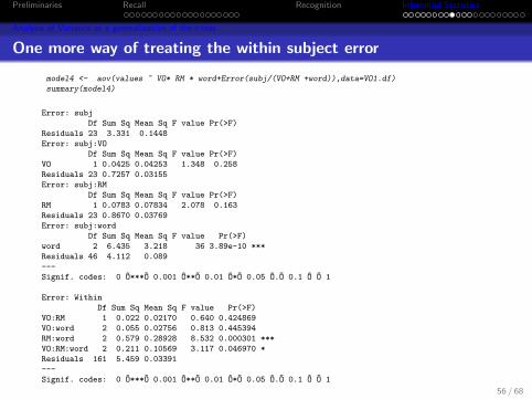
One more way of treating the within subject error
model4 <- aov(values ~ VO* RM * word+Error(subj/(VO+RM +word)),data=VO1.df)
summary(model4)
Error: subj
Df Sum Sq Mean Sq F value Pr(>F)
Residuals 23 3.331 0.1448
Error: subj:VO
Df Sum Sq Mean Sq F value Pr(>F)
VO 1 0.0425 0.04253 1.348 0.258
Residuals 23 0.7257 0.03155
Error: subj:RM
Df Sum Sq Mean Sq F value Pr(>F)
RM 1 0.0783 0.07834 2.078 0.163
Residuals 23 0.8670 0.03769
Error: subj:word
Df Sum Sq Mean Sq F value Pr(>F)
word 2 6.435 3.218 36 3.89e-10 ***
Residuals 46 4.112 0.089
---
Signif. codes: 0 O***~O 0.001 O**~O 0.01 O*~O 0.05 O.~O 0.1 O ~O 1
Error: Within
Df Sum Sq Mean Sq F value Pr(>F)
VO:RM 1 0.022 0.02170 0.640 0.424869
VO:word 2 0.055 0.02756 0.813 0.445394
RM:word 2 0.579 0.28928 8.532 0.000301 ***
VO:RM:word 2 0.211 0.10569 3.117 0.046970 *
Residuals 161 5.459 0.03391
---
Signif. codes: 0 O***~O 0.001 O**~O 0.01 O*~O 0.05 O.~O 0.1 O ~O 1
56 / 68

Preliminaries Recall Recognition Inferential Statistics
Analysis of Variance as a generalization of the t-test
What have we found?
1 One reliable (“statistically significant”) effect is that Correctwords are recognized more than False Words (Foils). This isnot overly surprising.
2 Another finding is that Recall or Math instructions interactedwith word type.
There is weaker finding that Recall versus Math interactedwith Visual versus Oral instructions on word tipe.
3 Lets look at the means to understand what is happening.
We do this by the simple R command ofprint(model.tables(model4,“means”))
57 / 68
Preliminaries Recall Recognition Inferential Statistics
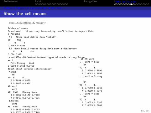
Analysis of Variance as a generalization of the t-test
Show the cell means
model.tables(model4,"means")
Tables of means
Grand mean # not very interesting don't bother to report this
0.7074653
VO #Does Oral differ from Verbal?
VO #no
O V
0.6953 0.7196
RM does Recall versus doing Math make a difference
M R #no
0.724 0.691
word #The difference between types of words is very large
word
Foil Strong Weak
0.5000 0.8464 0.7760
#What about various interactions?
VO:RM
RM
VO M R
O 0.7031 0.6875
V 0.7448 0.6944
VO:word
word
VO Foil Strong Weak
O 0.5052 0.8177 0.7630
V 0.4948 0.8750 0.7891
RM:word
word
RM Foil Strong Weak
M 0.5625 0.8021 0.8073
R 0.4375 0.8906 0.7448
VO:RM:word
, , word = Foil
RM
VO M R
O 0.5208 0.4896
V 0.6042 0.3854
, , word = Strong
RM
VO M R
O 0.7812 0.8542
V 0.8229 0.9271
, , word = Weak
RM
VO M R
O 0.8073 0.7187
V 0.8073 0.7708
58 / 68

Preliminaries Recall Recognition Inferential Statistics
Analysis of Variance as a generalization of the t-test
Or, show the cell “effects”
model.tables(model4,"effects")
VO
VO
O V
-0.012153 0.012153
RM
RM
M R
0.016493 -0.016493
word
word
Foil Strong Weak
-0.20747 0.13889 0.06858
VO:RM
RM
VO M R
O -0.008681 0.008681
V 0.008681 -0.008681
VO:word
word
VO Foil Strong Weak
O 0.017361 -0.016493 -0.000868
V -0.017361 0.016493 0.000868
RM:word
word
RM Foil Strong Weak
M 0.04601 -0.06076 0.01476
R -0.04601 0.06076 -0.01476
VO:RM:word
, , word = Foil
RM
VO M R
O -0.03819 0.03819
V 0.03819 -0.03819
, , word = Strong
RM
VO M R
O 0.01649 -0.01649
V -0.01649 0.01649
, , word = Weak
RM
VO M R
O 0.02170 -0.02170
V -0.02170 0.0217059 / 68
Preliminaries Recall Recognition Inferential Statistics
Graphing the interactions
There are multiple ways to graph the interaction
1 We can take the relevant means and just create a line graph
This does not show the error bars, although we can use theMean Square within subject residual to get an overall errorestimate.
2 Or, we can recode the data to combine the visual and oraldata and use error.bars. This is perhaps easier, but not asgeneral.
60 / 68
Preliminaries Recall Recognition Inferential Statistics
Graphing the interactions
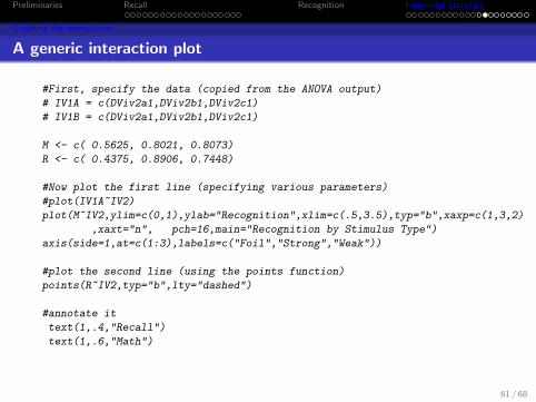
A generic interaction plot
#First, specify the data (copied from the ANOVA output)
# IV1A = c(DViv2a1,DViv2b1,DViv2c1)
# IV1B = c(DViv2a1,DViv2b1,DViv2c1)
M <- c( 0.5625, 0.8021, 0.8073)
R <- c( 0.4375, 0.8906, 0.7448)
#Now plot the first line (specifying various parameters)
#plot(IV1A~IV2)
plot(M~IV2,ylim=c(0,1),ylab="Recognition",xlim=c(.5,3.5),typ="b",xaxp=c(1,3,2)
,xaxt="n", pch=16,main="Recognition by Stimulus Type")
axis(side=1,at=c(1:3),labels=c("Foil","Strong","Weak"))
#plot the second line (using the points function)
points(R~IV2,typ="b",lty="dashed")
#annotate it
text(1,.4,"Recall")
text(1,.6,"Math")
61 / 68

Preliminaries Recall Recognition Inferential Statistics
Graphing the interactions
Recognition varies by Recall condition and word type0.0
0.2
0.4
0.6
0.8
1.0
Recognition by Stimulus Type
IV2
Recognition
Foil Strong Weak
Recall
Math
62 / 68

Preliminaries Recall Recognition Inferential Statistics
Graphing the interactions
Recoding the data to add error bars
for (dv in (1:6)) {pool.vo[,dv] <- (visualoral.df[,dv]+ visualoral.df[,dv+6])/2}
describe(pool.vo)
error.bars(pool.vo[,1:3],type="l",ylim=c(0,1),ylab="Recognition",xlab="Word Type",
main="Recognition Recall/Math and Word Type",xaxt="n",within=TRUE)
axis(side=1,at=c(1:3),labels=c("Foil","Strong","Weak"))
error.bars(pool.vo[,4:6],type="l",add=TRUE,within=TRUE,col="red")
vars n mean sd median trimmed mad min max range skew kurtosis se
FoilVr 1 24 0.44 0.28 0.50 0.44 0.28 0.00 0.88 0.88 -0.06 -1.06 0.06
StrongVr 2 24 0.89 0.14 0.88 0.91 0.19 0.50 1.00 0.50 -1.31 0.88 0.03
WeakVr 3 24 0.74 0.17 0.75 0.75 0.19 0.44 1.00 0.56 -0.24 -1.26 0.03
FoilVm 4 24 0.56 0.26 0.62 0.57 0.28 0.00 1.00 1.00 -0.37 -0.74 0.05
StrongVm 5 24 0.80 0.14 0.81 0.81 0.09 0.50 1.00 0.50 -0.48 -0.46 0.03
WeakVm 6 24 0.81 0.12 0.81 0.81 0.09 0.56 1.00 0.44 -0.08 -0.72 0.02
63 / 68

Preliminaries Recall Recognition Inferential Statistics
Graphing the interactions
Recognition varies by Word Type and Recall instructions
Recognition Recall/Math and Word Type
Word Type
Recognition
0.0
0.2
0.4
0.6
0.8
1.0
Foil Strong Weak
64 / 68

Preliminaries Recall Recognition Inferential Statistics
Graphing the interactions
Putting it all together
1 Recall
Although there was no effect of visual (mean = .73) versusoral (mean = .70) mode of presentation on recall(t23 = 1.63, p = .117), there was clear evidence for a serialposition effect (see Figure x). This showed that subjectsfollowed instructions to recall the last few words first.
2 Recognition
As expected, (False) recognition of foil words (.50) was lessthan that of the strongest associates (.85) or the weakerassociates in the middle of the list (.78) (F2,46 = 36, p < .001).While high associate words were recognized more followingprior opportunities to recall (.89) than not (.80), this effect wasreversed for the Foil words (.44 vs. .56, respectively) and forthe weaker associates (.74 vs .81) (F2,161 = 8.53, p < .001).
65 / 68

Preliminaries Recall Recognition Inferential Statistics
Graphing the interactions
Results for the paper
1 What is presented above is enough for the paper2 Probably include at least two figures -
serial position effectsRecognition by word type x Recall/math
3 Results should also include the inferential statistics
4 Additional analyses of recognition by strength of associate arenot included
66 / 68

Preliminaries Recall Recognition Inferential Statistics
Graphing the interactions
Structure of final paper (see detailed instructions from before)
1 Abstract (100-150 words)Why did you do the study, Who were the subjects, What didyou find, So what? Write it last.
2 Introduction (2-3 pages)A bit of background (adapt from R & M)Overview of study
3 Method (1-3 pages)With enough detail that someone can carry out the studyCan refer to word lists from R & M rather than including thewords
4 Results (1-3 pages)Just the most important resultsShould reference table(s) and figure(s) (to appear at end ofpaper)
5 Discussion (2-3 pages)Why is this study importantWhat are the most important findingsSo what? What is next
67 / 68


![SYLLABUS for Developmental Psychology COURSE NUMBER AND … · 2017-09-14 · 1 SYLLABUS for Developmental Psychology [v1] DATE: Fall 2017 COURSE NUMBER AND TITLE: PSYC 205-01 Developmental](https://static.fdocuments.net/doc/165x107/5e6b6986f46dcf319377f494/syllabus-for-developmental-psychology-course-number-and-2017-09-14-1-syllabus.jpg)